Embed Size (px)
Citation preview
Corruption Dynamics: The Golden Goose Effect∗
Paul Niehaus†
UC San DiegoSandip Sukhtankar‡
Dartmouth College
September 4, 2010
Abstract
Theoretical work on disciplining corrupt agents has emphasized promises of futurerents – for example, efficiency wages. This paper shows, theoretically and empirically,that illicit future rents have analogous incentive effects. When opportunities for futurerent extraction increase, agents extract less rent today in order to preserve those oppor-tunities. We study this “golden goose” effect in the context of India’s vast National RuralEmployment Guarantee Scheme. We compare official micro-records to original householdsurvey data to measure corruption and trace out the impacts of an exogenous increasein the scheme’s statutory wage to test the theory. We estimate that golden goose effectsreduced the total elasticity of theft with respect to this shock by roughly 70%. This sug-gests that dynamics should be taken into consideration when calibrating incentives. Italso advocates caution in interpreting policy experiments, since short-run trials generatedifferent dynamic incentives than permanent implementation. Finally, the results provideindirect support for models of electoral discipline and for the efficiency wage hypothesisitself
JEL codes: D73, H53, J30, K42, O12 Keywords: corruption, principal-agent problems,
dynamics, workfare
∗We thank Nageeb Ali, Eric Edmonds, Edward Glaeser, Roger Gordon, Claudia Goldin, Gordon Han-son, Larry Katz, Asim Khwaja, Michael Kremer, Sendhil Mullainathan, Ben Olken, Rohini Pande, AndreiShleifer, Jonathan Zinman, and seminar participants at Harvard, Yale, BREAD, Stanford, the World Bank,CGD, UNH, Indian Statistical Institute-Delhi, NEUDC-Boston University, Dartmouth, and UCSD for help-ful comments. Thanks also to Manoj Ahuja, Arti Ahuja, and Kartikian Pandian for generous hospitalityand insight into the way NREGS operates in practice, and to Sanchit Kumar for adept research assistance.We acknowledge funding from the National Science Foundation (Grant SES-0752929), a Harvard WarburgGrant, a Harvard CID Grant, and a Harvard SAI Tata Summer Travel Grant. Niehaus acknowledges sup-port from a National Science Foundation Graduate Student Research Fellowship; Sukhtankar acknowledgessupport from a Harvard University Multidisciplinary Program in Inequality & Social Policy Fellowship.†Department of Economics, University of California at San Diego, 9500 Gillman Drive #0508, San Diego,
CA 92093-0508. [email protected].‡Department of Economics, Dartmouth College, 326 Rockefeller Hall, Hanover, NH 03755.
1
1 Introduction
Disciplining corrupt officials is a key governance challenge in developing countries. In an
influential early analysis, Becker and Stigler (1974) argued that if there is some chance of
catching and dismissing corrupt agents then the problem can be mitigated by promising
them an efficiency wage. Intuitively, agents have an incentive to cheat less today in order
to improve their chances of earning wage premia tomorrow. This insight undergirds much
theoretical work on corruption.1
Our analysis begins with the simple observation that, in the Becker-Stigler framework,
illicit rents should play a role analogous to licit wage premia. For example, agents have
an incentive to cheat less today if this improves their chances of being able to extract
bribes tomorrow. We call this the “golden goose” effect: agents wish to preserve the goose
that lays the golden eggs (not kill it, as did the deplorably myopic farmer in the fable).2
It is a dynamic effect in the sense that it arises when agents have repeated opportunities
for corruption over time, so that one-shot models of corruption cannot capture it. In
fact, as we illustrate in the model below, the static effects of policy changes tend to have
offsetting dynamic effects.
This paper defines the golden goose effect theoretically and then quantifies its im-
portance. Bureaucratic jobs in which opportunities for corruption repeat themselves are
ubiquitous, but consistently measuring corruption is an empirical challenge.3 We work
in the context of India’s largest rural welfare program, the National Rural Employment
Guarantee Scheme (NREGS). The scheme entitles every rural household in India to up to
100 days of paid employment per year, provided only that they are willing to do manual la-
bor. The key feature for our purposes is that we were able to obtain disaggregated official
records on participation, including the names and addresses of participating households,
the duration of every spell of employment and the amount of compensation paid. Sam-
pling from these records, we conducted an independent survey of (alleged) beneficiaries.
We can then compare the amount of work that local officials claimed was done and the
amount of money those officials claimed as spent on reimbursing workers to independent
measures of work actually done and compensation actually received. The gap between
official and actual quantities – including over-reporting of days and under-payment of
wages – is the primary form of corruption we study
To test whether this form of corruption responds to variation in anticipated rent-
extraction opportunities we need an exogenous source of variation in the latter. We
1See Cadot (1987), Andvig and Moene (1990), Besley and McLaren (1993), Mookherjee and Png (1995),and Acemoglu and Verdier (2000), among others.
2Our usage thus differs from that of McMillan (2001), who uses the term “golden goose” to refer toex-ante investments by individuals that a government cannot commit not to hold up ex-post. Commitmentwill not be an issue in our setting.
3See Olken (2009) on the reliability of perceptions measures of corruption.
2
exploit a policy shock: a 1 May 2007 increase in the statutory wage due to program
participants in the state of Orissa. A higher statutory wage meant more lucrative corrup-
tion opportunities for officials, since they received more money for every fictitious day of
work reported. Importantly, the wage reform was enacted by policy-makers well removed
from the officials we study, making it plausibly exogenous. Moreover, because the wage
increase was specific to the state of Orissa, we can use data from the neighboring state
of Andhra Pradesh as a control in some specifications.
How does a wage change help us identify golden goose effects? In Section 3 we develop
a formal model of NREGS corruption which shows how the effects of the wage change
can be decomposed into a static price effect and a dynamic golden goose effect. The price
effect is straight-forward: when officials receive more money for every day of wage work
they report, they tend to report more fictitious days of wage work. But since the wage
change was permanent they also anticipate a more lucrative future, and this dynamic
effect tends to make them more conservative. The net effect on daily wage over-reporting
is thus ambiguous.
To separate the price effect and the golden goose effect we exploit an additional
institutional feature of our environment: roughly 30% of the NREGS projects in our study
area operated on a piece rate basis, rather than a daily wage one. Different projects used
different payment schemes because piece rates could not be implemented on projects
where worker output is hard to measure. The list of projects to be implemented had
been fixed in advance of the 1 May 2007 wage change, and piece rate schedules were
not revised along with the daily wage, so this reform should not have directly affected
piece rate projects. However, many officials who were managing piece rate projects at the
time of the shock also had daily wage projects planned for the near future. Consequently
they should have anticipated an increase in future rents. Moreover, this effect should
have been stronger for officials with a higher proportion of daily wage projects upcoming.
The model thus predicts that the wage increase should (1) reduce theft from piece rate
projects, and (2) differentially reduce corruption in areas with more daily wage projects
upcoming.
We take these predictions to panel data on corruption before and after the policy shock
in 215 panchayats (villages). We find that prices do matter: when statutory daily wages
increase, officials report more fictitious work on wage projects. None of the increase
in the statutory wage passed through to the wages actually received by workers, and
consequently the supply of labor to NREGS projects was unaffected. Overall, the daily
wage increase from Rs. 55 to Rs. 70 (combined with secular trends) increased the cost
to the government per dollar received by beneficiaries from $4.08 to $5.03.
Within this broad picture, however, we also find the two forms of evidence for golden
goose effects predicted by the model. First, theft on piece rate projects in Orissa declined
3
after the shock, both in absolute terms and relative to neighboring Andhra Pradesh.
Second, both daily-wage overreporting and piece rate theft were differentially lower after
the wage increase in the parts of Orissa which subsequently executed the most daily wage
projects — i.e. areas where the shock had the greatest impact on future rent expectations.
Rough calculations imply that the wage increase raised theft by approximately 70% less
than it would have had it been temporary, and thus not affected future rent expectations.
We consider a variety of alternative explanations for these results. Alternative mech-
anisms generally imply time-symmetry : the effects of future rent expectations should be
similar to the effects of past and current rent realizations. For example, if the marginal
value of rents is decreasing then officials who have extracted large rents in the past should
be conservative, just like officials who expect to extract large rents in the future. Em-
pirically, however, we find a robust role only for the future. We also test directly for
confounding changes in the intensity with which implementing officials were monitored
by their superiors and find no evidence thereof.
Understanding golden goose effects is important for predicting the impact of anti-
corruption policies. Consider increasing the steady-state probability that an agent will
be audited: as is well-known, the static effect of this change is to make illicit behavior
less attractive. But the same argument applies in the future as well, so that expected
future illicit rents will decrease. This in turn lowers the continuation value to the agent of
keeping his job, which makes any kind of illicit behavior today more attractive – he may
steal less on the margin being audited but more on other margins. Golden goose effects
thus provide the general lesson that static and dynamic effects tend to offset each other,
as well as an alternative explanation for “displacement effects” such as those documented
by Yang (2008).
Golden goose effects also influence the interpretation of policy pilots, in which dy-
namic effects differ from those generated by perpetual implementation. For example,
distributing welfare benefits once does not generate dynamic disincentives for theft,
but distributing them repeatedly does. A pilot may therefore appear to perform arti-
ficially poorly. Conversely, a one-shot crackdown on corruption does not affect future
rent expectations and may thus be more effective than a program of perpetual audits.
Understanding dynamics is thus important for interpreting the literature on the im-
pacts on corruption of monitoring (Di Tella and Schargrodsky 2003, Nagin, Rebitzer,
Sanders and Taylor 2002, Olken 2007) and of transparency more generally (Reinikka and
Svensson 2005, Ferraz and Finan 2008).
Since the golden goose effect and the efficiency wage effect both work through expec-
tations of future rents, our results provide indirect support for efficiency wage theories,
which have proved difficult to test (Di Tella and Schargrodsky (2003) being the notable
exception). Moreover, given that some of the officials implementing NREGS are elected,
4
our results support the leading models of electoral discipline, in which the need to promise
politicians some future rents puts a limit on how well voters can control their behavior
(Barro 1973, Ferejohn 1986, Persson, Roland and Tabellini 1997, Ahlin 2005, Ferraz and
Finan 2009).
In documenting the extent and nature of corruption in the NREGS we contribute to
the literature on the costs of corruption, which include the inability to remedy market
failures (Bertrand, Djankov, Hanna and Mullainathan 2007) and to redistribute wealth
(Reinikka and Svensson 2004, Olken 2006). These results are directly relevant in the
Indian policy context, where the NREGS plays a central role and is a volatile political
issue with much of the debate centering on leakage.
The rest of the paper is structured as follows: Section 2 describes the NREGS context,
Section 3 lays out the theoretical framework, Section 4 describes data collection and
estimation equations, Section 5 presents results, and Section 6 concludes.
2 Contextual Background on the NREGS
India’s National Rural Employment Guarantee Act is a landmark effort to redistribute
income to the rural poor. The program was launched in February 2006 in the poorest
100 districts in India and as of April 2008 covers the entire country (604 rural districts).
The total proposed budget allocation for the 2010-2011 fiscal year is Rs. 401 billion (US$
8.9 billion), which is 0.73% of 2008 GDP.4 It is likely that the steady-state cost will be
higher as implementation is still incomplete in many parts of the country.
2.1 Statutory Operational Procedures
Each operational program cycle begins before the start of a fiscal year, when local gov-
ernments at the Gram Panchayat (GP or panchayat, lowest level of administration in the
Indian government, comprising of a group of villages) and block (intermediate level of
government between GPs and districts) levels plan a “shelf” of projects to be undertaken
during the upcoming year. The particular types of project allowed under the NREGS
are typical of rural employment projects: road construction and earthworks related to
irrigation and water conservation predominate.
Projects also vary in the payment scheme they utilize: NREGS workers can be paid
either on a daily wage or a piece rate basis depending on the practicality of measuring
output. Our conversations with low-level officials in Orissa indicated that the decision
about how to pay workers is generally made on a project-by-project basis and by officials
4Costs: http://indiabudget.nic.in/ub2010-11/bh/bh1.pdf. GDP: http://mospi.nic.in/4_
gdpind_cur.pdf. The central government must by law contribute at most 90% of total expenditure, therest of the funding coming from the states.
5
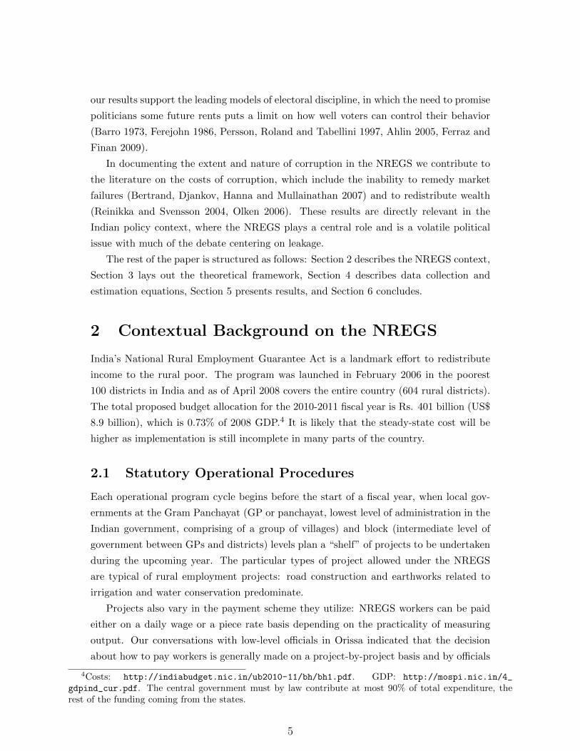
Figure 1: Distribution of Project TypesDistribution of Project Types
Fraction of spells paid a daily wage
Fre
quen
cy
0.0 0.2 0.4 0.6 0.8 1.0
020
040
060
0
Plots distribution of projects in study panchayats by the fraction of spells of (reported) work done that were
daily wage spells. Work spells are coded as daily wage spells if the payment per day is one of the statutory
daily wages. (Orissa implements four different daily wages for varying skill levels.)
at the block level. Empirically it is the case that all the work done on any particular
project is generally compensated in the same manner (see Figure 1). Consequently there
are identifiable daily wage projects and piece rate projects. While according to statute
the project shelf should be proposed by village assemblies (Gram Sabhas), in practice
higher up officials at the Block and District level suggest and approve the shelf.
A key feature of the NREGS is that it is an unrestricted entitlement program: every
household in rural India has a right to 100 days of paid employment per year, with no
eligibility requirements.5 To obtain work on a project, interested households must first
apply for a jobcard.6 The jobcard contains a list of household members, some basic
demographic information, and blank sheets for recording work and payment history. In
principle, any household can obtain a jobcard for free at either the panchayat or block
administrative office. Jobcards in hand, workers can apply for work at any time. The
applicant must be assigned to a project within 15 days after submitting the application,
if not they are eligible for unemployment compensation. Applicants have no influence
over the choice of project.
5Consequently officials do not have an opportunity cost of allocating work to workers, as in Banerjee(1997).
6Since each household is limited to 100 days of employment per year the definition of a household isimportant. In NREGS guidelines a household is “a nuclear family comprising mother, father, and theirchildren, and may include any person wholly or substantially dependent on the head of the family”. (Ministryof Rural Development 2008)
6
At the work sites the panchayat officials record attendance (in the case of daily wage
projects) or measure output (in the piece rate case). They record this information both
in workers’ jobcards and in muster rolls which are sent to Block offices and digitized.
The state and central governments reimburse local governments on the basis of these
electronic records. Most workers in our study area receive their wages in cash from the
panchayat administration, although efforts to pay them through banks are under way. As
a transparency measure, all the official micro-data on payments have been made publicly
available through a web portal maintained by the central Ministry of Rural Development
(http://nrega.nic.in).
2.2 Implementing Officials
The officials in charge of implementing the program are mainly appointed bureaucrats
at the block (Block Development Officers, Junior Engineers, Assistant Engineers) and
panchayat (Panchayat Secretary, Field Assistants, Mates, etc) levels, with the exception
of the elected chairman of the Gram Panchayat (the “Sarpanch”). The work of these
officials is overseen by district level program officials, including the District Collector.
While officials can be fired, suspended, or removed from their jobs for misconduct, Article
311(2) of the Indian constitution says that no civil servant can be dismissed without an
official enquiry, which makes it difficult to fire someone outright. However, suspensions
and transfers into backwater jobs are common punishments (Das 2001).
Because our analysis revolves around forward-looking optimization it is useful to un-
derstand bureaucratic tenure in these jobs. Tenure is typically short, primarily because
transfers are used as a disciplinary tool and as a way for political parties to bestow fa-
vors. Iyer and Mani (2009) document that the district-level Indian Administrative Service
(IAS) officers who oversee local officials stay in a job for a year and a half on average, and
since they often move with their staff this implies that the tenure of lower-level officials is
at least as short. In Gujarat, Block Development Officers keep that post for an average
of sixteen months (Zwart (1994), p 94). Given the small but significant pay differential
between private sector and public sector jobs at this level (Das 2001) and the short tenure,
local public officials often seek opportunities for extracting rents.
2.3 Opportunities for Rent Extraction
Officials’ opportunities for illicit gain include control over project selection; bribes for
obtaining jobcards and/or employment; and embezzlement from the materials and labor
budgets. We focus on theft from the labor budget, which we can cleanly measure. The
labor budget is required by law to exceed 60% of total spending, and in fact we find that
theft in this category is so extensive that even if all of the 40% allocated to materials
7
were stolen, the labor budget would still be the larger source of illegal rents.7
Theft from the labor budget comes in two conceptually distinct forms. First, officials
can under-pay workers for the work they have done (theft from beneficiaries). Second,
officials can over-report the amount of work done when they send their reports up the
hierarchy (theft from taxpayers).8
2.4 Monitoring and Enforcement
A key difference between theft from beneficiaries and theft from taxpayers lies in the
way they are monitored. Underpaid workers who know they are underpaid could poten-
tially complain to someone at the block or district headquarters.9 On the other hand,
workers have little incentive to monitor over-reporting: because the program’s budget
is not fixed, a rupee stolen through over-reporting does not mean a rupee less for the
workers. Realistically, then, over-reporting must be monitored from the top down. The
NREGS Operational Guidelines (Ministry of Rural Development 2008) call for both top-
down monitoring, via internal verification of works by officials (100% works audited at
the block level, 10% by district level monitors, and 2% by state level monitors), and
bottom-up monitoring via Gram Sabhas (village meetings), local Vigilance and Monitor-
ing Committees, as well as bi-annual “social audits” done by civil society. In practice
we saw that block and district officials use the NREGS’s management information sys-
tem (MIS) to track aggregate quantities of work done on various projects and compare
these to technical estimates or to their own intuitions about how much work should be
necessary.
Officials caught cheating face a low but positive probability of getting caught. Program
guidelines call for “speedy action against [corrupt] officials” but do not lay out specific
penalties. In practice the most likely penalty is suspension or transferal to a less desirable
job; for elected officials it is loss of office.10 The strength of enforcement in Orissa is
7We also found that bribes paid to obtain jobcards are uncommon (17% report paying positive amounts)and small (averaging Rs. 10 conditional on being positive). This is not surprising given that (1) a jobcardis an entitlement and not receiving a jobcard is a relatively verifiable event; (2) households can apply toeither the panchayat or the block office, which potentially creates bribe-reducing competition (Shleifer andVishny 1993); (3) the NREGS places no limit on the number of participants, so officials actually havepositive incentives to sign up participants. Note that this last feature implies that there is less scope forcorruption to “grease the wheel,” or improve efficiency by getting around cumbersome red tape or regulations(Leff 1964, Huntington 1968).
8For example, a worker who worked for 10 days on a daily wage project when the statutory minimumwage was Rs. 55 per day might receive only Rs. 45 per day in take-home pay. The official might report thatthe worker had worked for 20 days rather than 10. His total rents would then equal 55 · 20 − 45 · 10 = 650rupees, the sum of the two sorts of theft.
9In practice, however, only 7% of respondents said they would complain to one of these officials if theyhad a problem, because of the costs of complaining (53%) and the low probability that a complaint wouldbe successful (37%). See Niehaus and Sukhtankar (2010) for details.
10It is important to note that the theoretical predictions of our model do depend qualitatively on whether
8
difficult to quantify; the Chief Minister at one point claimed to have initiated action
against nearly half the Block Development Officers in the state, but some of this is likely
political posturing.11 A more reliable source may be the records of OREGS-Watch, a
loose online coalition of non-governmental organizations that monitor NREGS in Orissa;
their reports note numerous instances of officials being caught and suspended (http:
//groups.google.co.in/group/oregs-watch). The common pattern in these cases was
incontrovertible proof brought to the office of the District Collector, followed immediately
by the suspension of the guilty official and in some cases by the recovery of the stolen
funds. In one case in Boudh district, for example, the offending official was caught
within two weeks of the misdemeanor, the money recovered and the official suspended.12
Andhra Pradesh has systemized the process of social audits, creating a quasi-government
“Society” for Social Audits (http://www.socialauditap.com) that conducts door-to-
door verification of muster rolls, which has succeeded in recovering over Rs. 130 million
in stolen funds.
2.5 The Political Economy of Wage-Setting
Our estimation strategy below exploits an increase in statutory program wages in the
eastern state of Orissa in 2007. Such wage hikes were common due to the incentives
generated by the NREGS’s funding pattern. The central (federal) government pays 100%
of the unskilled labor budget, and 75% of the materials budget (defined to include the
cost of skilled labor) (Ministry of Law and Justice 2005). However, the states set wages
and piece-rates. This provision – possibly intended to allow flexibility to adapt program
parameters to local labor market conditions – creates strong incentives for state politicians
to raise wage rates, benefiting their constituents at the central government’s expense. We
study the effects of a change in the statutory daily wage in Orissa from Rs. 55 to Rs.
70. This change was announced on April 28th, 2007 and went into effect on May 1st,
2007. Two key features of this policy change are that it did not directly affect payments
on piece rate projects and that it was specific to Orissa and did not affect neighboring
Andhra Pradesh.
the punishment is suspension, transfer, or permanent dismissal. Similarly, some degree of collusion betweenlocal officials and their monitors would not change the qualitative predictions.
11http://www.orissadiary.com/Shownews.asp?id=620112http://www.dailypioneer.com/59458/Action-taken-after-study-finds-fake-muster-roll-in-Boudh.
html.
9
3 Dynamic Rent Extraction
Following the seminal work of Becker and Stigler (1974), a large theoretical literature has
studied the use of dismissal threats to motivate corruptible agents. In this section we
adapt the Becker-Stigler model to our setting and draw out the role that illicit future rents
play in shaping the agent’s decision-making. The driving assumptions are that the chance
the official is caught and punished increases in the amount of corruption he engages in,
and that the penalty for being caught is dismissal. We adapt the model to our context by
explicitly modeling the distinct forms of corruption that we measure empirically: over-
reporting on daily wage projects, under-payment on daily wage projects, and aggregate
theft on piece-rate projects. We will show how combining standard theoretical elements
with these margins yields testable predictions about the effects of a statutory wage change.
Time is discrete. An infinitely-lived official and a group of N infinitely-lived workers
seek to maximize their discounted earnings stream:
ui(t) =∞∑τ=t
βτ−tyi(τ) (3.1)
where yi(τ) are the earnings of agent i in period τ . Additional players with identical
preferences wait in the wings to replace the official should he be fired.
In each period exactly one NREGS project is active. We abstract from simultaneous
ongoing projects primarily to simplify the exposition; it is also true, however, that most
of the panchayats in our sample have either one or zero projects active at all times during
our study period. Let ωt = 1 indicate that the active project at time t is a wage project,
and ωt = 0 that it is a piece rate project. We represent the “shelf” of projects as an
infinite stochastic stream of projects: at the beginning of each period a random project
is drawn from the shelf with
φ ≡ P(ωt = 1|ωt−1, ωt−2, . . .) (3.2)
We suppose that all agents know φ but do not know exactly which projects will be imple-
mented in the future. At the cost of a small loss of realism, this approach ensures that the
dynamic environment is stationary and greatly simplifies the expression of comparative
statics. It also permits a close analogy between the model and our empirical work, in
which the fraction of future projects that are daily wage (a measure of φ) plays a key
role. We treat φ as exogenous here since de jure it should be predetermined for our study
period, but we will also check in our empirical work that it does not respond to the wage
change.
Each worker inelastically supplies one indivisible unit of labor in each period. We will
interpret a unit flexibly as either a day (in the case of daily wage projects) or as a unit of
10
output (in the case of piece-rate projects). Labor may be expended on an NREGS project
or in the private sector, where worker i can earn wt (rt). Let nt (qt) be the number of
days (output units) supplied to the project when ωt = 1 (ωt = 0), and let and wti (rti)
be the wage (piece-rate) that participating worker i receives. This need not equal the
statutory wage w (the statutory piece rate r).
NREGS wages and employment levels emerge from bargaining between the official
and the workers. As we show in a companion paper (Niehaus and Sukhtankar 2010),
participants NREGS wages (wti) and their participation choices (nt) are determined by
the prevailing market wage rate wt in the village and are not affected by the statutory
NREGS rate w. Thus while in principle labor supply nt depends on the official’s wage
offers {wti} we ignore this dependence since wti = wt for all (i, t). We further simplify
matters by abstracting from time variation in the market wage, so wt = w and nt = n.
Participation n and the average participant’s wage w (piece rate r) are thus predeter-
mined once the official chooses how much work n̂t to report. If the current project is a
wage project, official’s period t rents will be
yto(ωt = 1) = (w − w)︸ ︷︷ ︸
Under-payment
n+ (n̂t − n)︸ ︷︷ ︸Over-reporting
w
and analogously if it is a piece-rate project,
yto(ωt = 0) = (r − r)︸ ︷︷ ︸
Under-payment
q + (q̂t − q)︸ ︷︷ ︸Over-reporting
r
Over-reporting the amount of work done puts the official at risk of being detected by a
superior and removed from office. The probability of detection on daily wage projects is
π(n̂, n), with π(n, n) = 0 for any n, π1 > 0, π2 < 0, and π11 > 0 for all n; the last condition
ensures an interior equilibrium amount of over-reporting. We also assume that if n > n′
then π((n+x), n) ≤ π((n′+x), n
′). This condition ensures that officials weakly prefer to
have more people work on the project; it would be satisfied if, for example, the probability
of detection depended on the total amount of over-reporting or on the average rate of
over-reporting. The probability of detection on piece rate projects is µ(q̂t, q) with entirely
analogous properties. If an official is caught we assume that he is removed from office
before the beginning of the next period and earns some fixed outside option normalized
to zero in every subsequent period. In practice corrupt officials are sometimes suspended
11
rather than fired; modeling this would affect our results only quantitatively.1314
The recursive formulation of the official’s objective function is
V (w, φ) ≡ φV (w, 1, φ) + (1− φ)V (w, 0, φ)
V (w, 1, φ) ≡ maxn̂
[(w − w)n+ (n̂− n)w + β(1− π(n̂, nt))V (w, φ)
]V (w, 0, φ) ≡ max
q̂
[(r − r)q + (q̂ − q)r + β(1− µ(q̂, qt))V (w, φ)
]where V (w, 1) is the official’s expected continuation payoff in a period with a daily wage
project, V (w, 0) is his expected continuation payoff in a period with a piece rate project,
and V (w) is his expected continuation payoff unconditional on project type.
We first derive the official’s response to a temporary, one-period change in the statu-
tory daily wage. These are not testable predictions, since the wage change we study below
was a permanent one. Rather, because they coincide with the predictions a static one-
period model would deliver, they help highlight the consequences of modeling dynamics.
Proposition 1. A one-period increase in the statutory daily wage w
• Increases over-reporting on daily wage projects (n̂t − n)
• Has no effect on theft from piece rate projects (q̂tr − qr)
These results are straightforward to derive because the official’s continuation value
V (w, φ) is not affected by a temporary wage change – one can think of it as analogous
to the pension that Becker and Stigler (1974) proposed giving to officials who complete
their careers without incident. Because this quantity is fixed the wage change acts like a
pure price shock for officials managing daily wage projects: the value of over-reporting a
day of work goes up, while the cost is unaffected. Consequently over-reporting increases.
As for officials managing a piece-rate project, neither the costs nor the benefits of stealing
have changed.
When the statutory wage changes permanently this generates both the static effects
above and also dynamic effects working through changes in the official’s continuation
value V (w, φ). This can potentially reverse the model’s predictions for daily wage over-
reporting unless an inelasticity condition holds:
13Officials may also leave their posting for more benign reasons – a bureaucrat may be reassigned or apolitician’s term may expire. Modeling this possibility would yield additional predictions: a bureaucratnear the end of his term may have weaker incentives to avoid detection, as suggested by Olson (2000).Unfortunately our data do not include variation in tenure, and so for simplicity we omit it from the modelas well.
14Detected officials may also be forced to repay some of what they have stolen. If this were possible itshould make officials who have stolen a great deal in the past more conservative. To the extent that we cantest this channel with our data, the opposite appears to be true, as officials who had more opportunities tosteal in the past (a higher fraction of daily-wage project-days) steal more now.
12
Proposition 2. Over-reporting n̂t−n on daily wage projects is increasing in w if wV∂V∂w <
1 and decreasing otherwise.
Proof. All proofs are deferred to Appendix A.
This prediction is ambiguous because a higher statutory wage has two offsetting ef-
fects. The first is the price effect identified above: a higher wage increases the benefit
of over-reporting. The second is a golden goose effect: a higher wage raises the value of
future over-reporting, which in turn increases the importance of keeping ones job. The
former effect dominates only if the elasticity of future benefits with respect to the wage
is sufficiently small. This tension between static and dynamic effects is a general feature:
any increase in the “scope” for rent extraction – new opportunities, lower costs, weaker
monitoring – will have a direct tendency to increase rent extraction, but will also raise
the continuation value of the game to corrupt officials, which will tend to reduce current
rent-extraction.
While it illustrates this tension, Proposition 2 also implies that over-reporting of daily
wage work is not a useful outcome variable with which to test the theory. One way to
obtain a test is to look at effects on forms of rent extraction that are not directly affected
by the wage increase, such as theft from piece-rate projects.
Proposition 3. Total theft from piece-rate projects (q̂tr − qr) is decreasing in w.
Here we obtain an unmitigated golden goose effect. A higher statutory wage has no
effect on current rent-extraction opportunities for a bureaucrat managing a piece-rate
project. It does, however, increase expected future rent extraction opportunities, which
discourages theft.
We can construct an additional test by exploiting cross-sectional variation in the
intensity with which the wage change affects official’s future rent expectations. Since the
wage change only affects rents in future periods during which a wage project is running,
one might expect to see differentially stronger effects in places with more future wage
projects upcoming (higher φ). As it turns out things are not quite this simple: if piece
rate and daily wage projects are not equally lucrative then there may be additional sources
of treatment heterogeneity working through these “wealth effects”. If the rents from piece
rate and daily wage projects are approximately the same, however, we get the prediction
one intuitively expects:
Proposition 4. Restrict attention to any closed, bounded set of parameters (φ,w, r, w, r).
Then for |yo(1)− yo(0)| sufficiently small,
∂2(n̂t − n)
∂w∂φ< 0 and
∂2(q̂tr − qr)∂w∂φ
< 0
13
In our empirical work we will first verify that equilibrium rents from daily wage and
piece rate projects are similar, and then test this prediction.
3.1 Confounding Explanations
While the predictions above are testable, they are not necessarily unique to our model.
One potential confound involves the “production function” for corruption. We believe
that the bulk of corruption in our setting simply involves writing one number on paper
instead of another. Suppose, however, that this requires the use of some scarce input
that can be shifted across time (e.g. effort). Then the wage shock would induce officials
to optimally re-allocate this input across time, giving rise to patterns similar to those
we predict. Second, if officials care about things other than consumption then the wage
shock might have income effects. The expectation of large future rents would lower the
expected relative marginal utility of income now, leading to lower corruption. Finally,
empirical tests could potentially be sensitive to issues of time aggregation. In our empir-
ical work we treat the day as the basic unit of time, but monitoring might be based on
less frequent observations. This would mechanically imply that officials expecting to steal
more tomorrow would steal less today, since the probability of detection would depend
on the sum of today’s report and tomorrow’s.
The key difference between the golden goose effect and each of these mechanisms
is that while the former is purely forward-looking, the latter are all time-symmetric.
For example, if officials who plan to expend a lot of effort stealing tomorrow steal less
today, then officials who have expended a lot of effort yesterday should also steal less
today. Similarly, if officials who expect large future income shocks care less about income
today, then so should officials who have already received large income shocks. Likewise,
if monitoring probabilities are based on weekly or monthly aggregates then corruption
today should on average be negatively related to both corruption tomorrow and corruption
yesterday.
4 Empirical Approach
4.1 Official Data
To test the theoretical predictions in Section 3 we adopt an audit approach, comparing
official micro-data on wage payments and program participation to original household
survey data collected from the same (alleged) beneficiaries. The official data we use are
publicly available on a central website (http://nrega.nic.in). Data available at the
level of the individual worker include names, ages, addresses, caste status, and unique
household jobcard number. Data available at the level of the work spell include number
14
of days worked, name and identification number of the project worked on, and amount
paid. Descriptive information on the nature of the projects and the names of the officials
responsible for implementation are also available. It is straight-forward to infer whether
a project paid daily wages or piece rates because there are only a few allowed daily wage
rates.15 (Figure 1)
An important point regarding the official records is that the 100-day-per-household
constraint essentially never binds. During fiscal year 2006-2007 only 4% of jobcards in
our study area in Orissa are recorded as having reached 100 days, and all panchayats had
a significant number of jobcards with less than 100 days – on average 95% of the cards
in the panchayat, and at a minimum 22%.
We used as our sample frame the official records for the states of Orissa and Andhra
Pradesh as downloaded in January 2008, six months after our study period to allow time
for all the relevant data to be uploaded. As a cross-check we also downloaded the official
records a second time in March 2008. We found that the records for Orissa remained
essentially unchanged, but that the number of work spells recorded for Andhra Pradesh
had increased by roughly 10%. These new observations were spread uniformly across
space and time and so do not appear to have resulted from delays in processing records
for specific panchayats or projects. They do, however, generate some uncertainty about
the appropriateness of our AP sample frame, and so we will emphasize the Orissa data
and use AP as a control only in Table 5.
We sampled from the list of officially recorded NREGS work spells during the period
March 1st, 2007 to June 30th, 2007 in Gajapati, Koraput, and Rayagada districts in
Orissa. Within these districts, we restricted our attention to blocks at the border with
AP. We sampled 60% of the Gram Panchayats within study blocks, stratified by whether
the position of GP chief executive had been reserved for women. (Chattopadhyay and
Duflo (2004) find evidence suggesting that these reservations affect levels of corruption.)
Within these panchayats we sampled 2.8 percent of work spells, stratified by Panchayat,
by whether the project was implemented by the block or the panchayat administration, by
whether the project was a daily wage or piece-rate project, and by whether the work spell
was before or after the daily wage shock. This yielded a total of 1938 households. We set
out to interview all adult members of these households about their NREGS participation,
so that our measures of corruption would not be affected if work done by one member
was mistakenly reported as having been done by another. Details on survey results and
a sample description are in Appendix B.
15These are Rs. 55, 65, 75, and 85 prior to the wage change, and Rs. 70, 80, 90 and 100 afterwards. Wedesignate a project as daily wage if more than 95% of the wages paid are these amounts. The higher wagesare paid for slightly higher-skilled work; these are very rare occurrences, and the overwhelming majority ofwages reported paid are Rs. 55 and Rs. 70.
15
4.2 Survey Content
We asked respondents retroactively about spells of work they did between March 1, 2007
and June 30, 2007. A spell of work is a well-defined concept within the NREGS: it is an
uninterrupted period of up to two weeks employment on a single project. For each spell
we asked subjects the dates during which they worked, the number of days worked, what
project they worked on, whether they were paid on a piece rate or daily wage basis, what
payment they received, and in the case of piece rate projects what quantity of work they
did. While recall of most of these variables is good, recipients have difficulty recalling the
quantity of work done on piece rate projects – the amount of earth they moved, volume
of rocks they split, etc. Consequently in our empirical work we treat theft on piece rate
projects as unitary – q̂tr − qtrt in terms of the model – keeping in mind that it includes
theft both from beneficiaries and from taxpayers. In addition to the survey of program
participants, we also asked a separate questionnaire to village elders with questions on
labor market conditions, agricultural seasons and official visits in the village.
While imperfect recall could potentially be a concern given the lag between the study
period and our survey, results were very encouraging. This is likely because the NREGS
was a new and very salient program, and spells of work were likely to be memorable and
distinct compared to other employment. Moreover, since participants do not necessarily
get paid what they are owed and often not on time, they are likely to keep track of how
much they worked and what they received. Finally, we designed the survey carefully to
prompt memory (e.g. using major holidays as reference points) and trained surveyors to
jog respondents’ memories. Consequently, we obtained information on at least the month
in which work was done for 93% of the spells in our sample. We do not find significant
differential recall problems over time: in a variety of specifications including location fixed
effects and individual controls such as age and education, subjects’ estimated probability
of recalling exact dates increases by only 0.7%–2.2% per month and is not statistically
significant. Since our main tests exploit discrete time-series changes while controlling for
smooth trends, these patterns should not introduce bias.
Survey interviews were framed to minimize other potential threats to the accuracy and
veracity of respondents self-reports. We made clear that we were conducting academic
research and did not work for the government, to discourage them from claiming fictitious
underpayment; in the end most respondents reported that they had been paid what
they thought they were owed. None of the interviewed households have income close to
the taxable level and will have ever paid income taxes, so there are no tax motives for
underreporting. Conversely, officials had little need to secure workers’ collusion in their
over-reporting. All a worker could possible supply would be a signature, which has little
relevance when most people cannot write their own name. There is also no reason to
believe that respondents would under-report corruption for fear of reprisals, since they
16
could not have known how many days they were reported as having worked in the official
data. Finally and most importantly, there is no reason to think any of these issues would
lead to differential biases (which would affect our results) and not just level ones (which
would not). Niehaus and Sukhtankar (2010) confirms that the wage shock had no effect
on the self-reported variables we use in our analysis.
4.3 Empirical Specifications
Our empirical analysis includes all spells of work from our survey data that contain
information on at least the month of the spell, the number of days worked, and the wages
received. We impute start or end dates if unavailable,16 and construct time-series of
survey reports of work done and wages paid by aggregating data at the panchayat-day
level for the sample period. Similarly, we construct time-series of the official data by
aggregating official reports of work done and wage paid of only those households who we
interviewed or confirmed as fictitious over the sample period.
We code the wage change as a simple dummy variable equal to 1 after May 1, 2007.
To control for periodicity in both actual and official reports of days worked (see Figure
3), and also any spurious correlations over time, we include various time trends and an
indicator for major public holidays. Because opportunities for corruption may depend
on how much work is ongoing we include non-parametric controls for number of days of
work actually done (DayCat), in the form of indicator variables for each number. Note
that while the model yields predictions for over-reporting (n̂t − n), we are allowing for
more flexible functional forms by including n non-parametrically on the right-hand side.
We also include district fixed effects (δ) in certain specifications. All standard errors are
two-way clustered by panchayat and day. To sum up, for outcome Y in panchayat p at
time t we have:
Ypt = β0 + β1Shockt + Time′tγ +DayCat
′ptφ+ δp + εpt (4.1)
Identification rests on the assumption that unobserved factors affecting the optimal
amount of theft are orthogonal to the shock Shockt after controlling for general time
trends.
We can relax this identifying assumption by using data from the neighboring district of
Vizianagaram in Andhra Pradesh to control for unobserved time-varying effects common
to the geographic region under study. This approach is, however, subject to several
caveats. First, we can only utilize it when estimating models of piece-rate theft, since
16We distribute days worked equally over the month if neither start nor end date are available, and equallyin the period between the start date and end date if the number of days worked is less than the period betweenthe start and end dates.
17
essentially all projects in Andhra Pradesh are piece rate. Second, as noted above a
substantial number of new observations appeared in the official Vizianagaram records
after we selected our sample. Finally, Andhra Pradesh made two revisions to its schedule
of piece rates during our sample period, the latter of which took effect on March 25th,
2007. Because of its proximity to the daily wage change in Orissa this shock limits the
value of Andhra Pradesh as a control for high-frequency confounds, although it may still
be useful for low-frequency ones.
Keeping these limitations in mind, we estimate
Ypt = β0 + β1ORshockt ∗ORp + β2APShock1t ∗APp + β3APShock2t ∗APp+ β4ORshockt + β5APShock1t + β6APShock2t +ORp
+ Time′ptγ +DayCat
′ptφ+ δp + εpt (4.2)
The coefficient of interest in this specification is β1, the differential effect of the post-
shock period ORshockt on corrupt behavior in Orissa, indicated by ORp. We control for
a variety of time and state-specific time trends.
To test Proposition 4 we need an empirical analogue to φ, the probability that a
future project in our model is a daily wage project. For each panchayat-day observation
we calculate the fraction FwdWageFrac of project-days in the upcoming two months that
are daily wage project-days. This time window appears reasonable given the relatively
short tenure (12-16 months) of appointed officials, but we will also report results using
one month and three month windows, which are not qualitatively different. We define a
“project-day” as a day on which a particular project is running, and define a project as
running if work on that project as been reported in the past and will be reported in the
future.
Our goal in constructing this variable is to capture variation in the proportion of
daily wage projects on the panchayat’s “shelf” of projects as cleanly as possible. While
the quantities of work reported or the amount of rents earned in the future are clearly
endogenous, the proportion of projects that are daily wage should not be if the project
shelf is fixed in advance as required by law. We test this idea below and show that our
measure of shelf composition is unaffected by the wage shock. Even if this were not the
case, we expect that biases would tend to work against us rather than for us: panchayats
that increased their corruption most in response to the shock would be the most likely
to switch to wage projects, generating a positive bias on the Shockt ∗ FwdWageFracpt
term. We thus test Proposition 4 by checking that β2 < 0 in the following estimation:
18
Ypt = β0 + β1Shockt + β2Shockt ∗ FwdWageFracpt + β3FwdWageFracpt
+ Time′tγ +DayCat
′ptφ+ δp + εpt (4.3)
Table 1 presents summary statistics of the main variables used in our regressions.
Table 1: Summary Statistics of Main Regression Variables
Mean SD ObsDW Days Official 3.31 6.30 13054DW Days Survey 0.88 1.55 13054PR Rate Official 94.08 259.70 7320PR Rate Survey 12.96 43.43 7320FwdWageFrac 0.67 0.40 13908
This table provides summary descriptions of the aggregated variables used in the main result tables 3 and
4. The sample for each kind of project includes panchayats that had at least one of that kind of project
active during the study period (March 1 through June 30 2007). “DW Days Official” is the days worked
by panchayat-day on daily wage projects as reported officially. “DW Days Survey” is the days worked by
panchayat-day on daily wage projects as reported by survey respondents. “PR Rate Official” is the total
payments by panchayat-day on piece rate projects as reported officially, while “PR Rate Survey” corresponds
to the same figure as reported by survey respondents. “FwdWageFrac” is the proportion of project-days in
the next two months in a panchayat that are daily wage.
5 Results: The Golden Goose Effect
5.1 Preliminaries: Wages, Quantities and Rents
We begin with a series of preliminary tests of the main identifying assumptions. First we
verify that the policy change was actually implemented; Figure 2 shows this clearly. The
average rate officially reported as being paid on daily wage projects stays fairly constant
near Rs. 55 up until May 1st and then jumps up sharply thereafter. Interestingly it does
not immediately or permanently reach the new statutory wage of Rs. 70, because not all
panchayats implemented the change – some continued to claim the old rates after May
1st, presumably because they were not informed about the change.17
Figure 2 also shows that the wage rate actually received by workers was unaffected by
the shock. (It appears to trend slightly downwards but this effect is largely compositional
17This interpretation suggests an additional test: all our predictions should hold only in panchayats thatactually implemented the wage change. We pursued this strategy, but unfortunately there are insufficientlymany non-implementing panchayats for us to precisely estimate the difference.
19
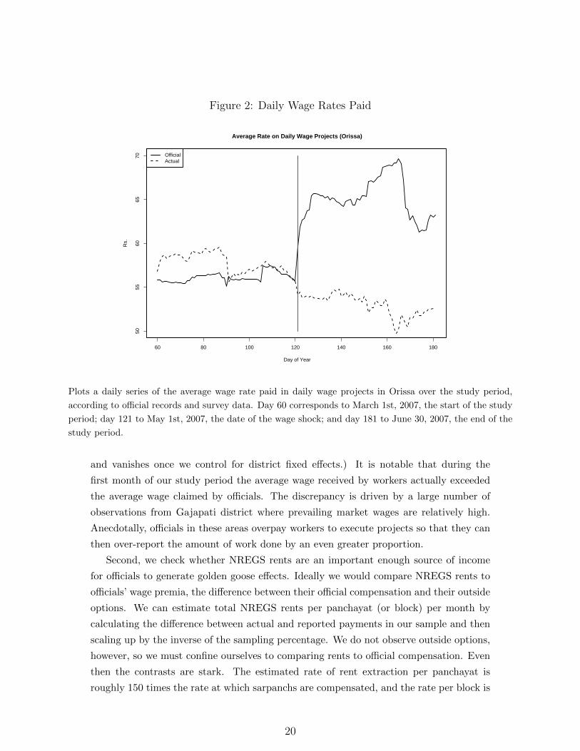
Figure 2: Daily Wage Rates Paid
60 80 100 120 140 160 180
5055
6065
70
Day of Year
Rs.
Average Rate on Daily Wage Projects (Orissa)
OfficialActual
Plots a daily series of the average wage rate paid in daily wage projects in Orissa over the study period,
according to official records and survey data. Day 60 corresponds to March 1st, 2007, the start of the study
period; day 121 to May 1st, 2007, the date of the wage shock; and day 181 to June 30, 2007, the end of the
study period.
and vanishes once we control for district fixed effects.) It is notable that during the
first month of our study period the average wage received by workers actually exceeded
the average wage claimed by officials. The discrepancy is driven by a large number of
observations from Gajapati district where prevailing market wages are relatively high.
Anecdotally, officials in these areas overpay workers to execute projects so that they can
then over-report the amount of work done by an even greater proportion.
Second, we check whether NREGS rents are an important enough source of income
for officials to generate golden goose effects. Ideally we would compare NREGS rents to
officials’ wage premia, the difference between their official compensation and their outside
options. We can estimate total NREGS rents per panchayat (or block) per month by
calculating the difference between actual and reported payments in our sample and then
scaling up by the inverse of the sampling percentage. We do not observe outside options,
however, so we must confine ourselves to comparing rents to official compensation. Even
then the contrasts are stark. The estimated rate of rent extraction per panchayat is
roughly 150 times the rate at which sarpanchs are compensated, and the rate per block is
20
a staggering 1,100 times the rate at which Block Development Officers are compensated.
Clearly the NREGS dominates official compensation as a source of income.
Third, we check whether pre-shock rent extraction from daily wage and piece rate
projects are similar, as predicated by Proposition 4. Dividing total theft in the two
categories of projects by the number of actual days worked on those projects, we find
that the rate of theft per day worked is very similar post-shock; Rs. 236 per actual day
worked in daily wage projects as opposed to Rs. 221 in piece rate projects.18
Table 2: Wage Shock Effects on Project Composition
Regressor I II IIIShock 0.024 0.022 0.024
(0.023) (0.023) (0.022)
Day 0 0.001 -0.002(0.001) (0.001) (0.003)
Day2 0.001(0.001)
District FEs N Y NReal Labor, Seasons Y Y YN 12103 12103 12103R2 0.017 0.025 0.017
This table presents regressions of the “FwdWageFrac” indicator, or the proportion of future project-days
(next two months) in a panchayat that are daily wage. “Shock” is an indicator equal to 1 on and after May
1, 2007. The variable Day represents a linear time trend. The variable Day2 has been rescaled by the mean
of Day. All columns include the following standard controls: non-parametric controls for number of days of
work actually done, a third-order polynomial in the day of the month, and indicators for major agricultural
seasons. Robust standard errors – multi-way clustered by panchayat and day – are presented in parenthesis.
Statistical significance is denoted as: ∗p < 0.10, ∗∗p < 0.05, ∗∗∗p < 0.01
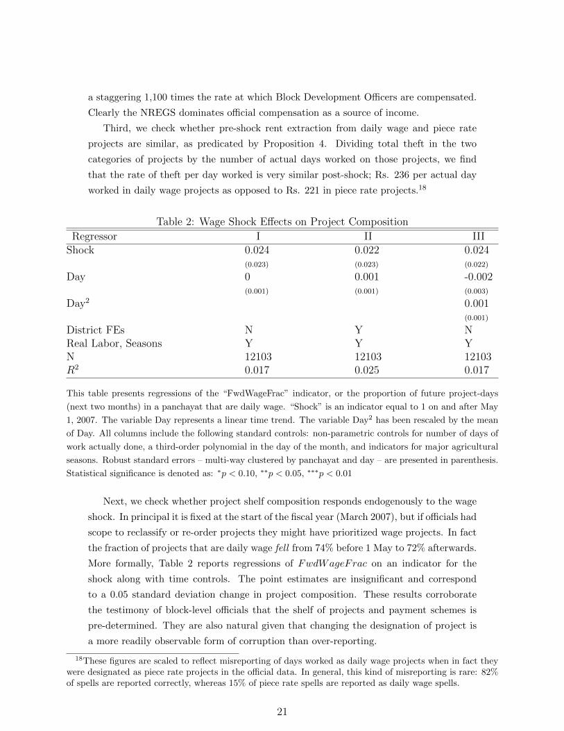
Next, we check whether project shelf composition responds endogenously to the wage
shock. In principal it is fixed at the start of the fiscal year (March 2007), but if officials had
scope to reclassify or re-order projects they might have prioritized wage projects. In fact
the fraction of projects that are daily wage fell from 74% before 1 May to 72% afterwards.
More formally, Table 2 reports regressions of FwdWageFrac on an indicator for the
shock along with time controls. The point estimates are insignificant and correspond
to a 0.05 standard deviation change in project composition. These results corroborate
the testimony of block-level officials that the shelf of projects and payment schemes is
pre-determined. They are also natural given that changing the designation of project is
a more readily observable form of corruption than over-reporting.
18These figures are scaled to reflect misreporting of days worked as daily wage projects when in fact theywere designated as piece rate projects in the official data. In general, this kind of misreporting is rare: 82%of spells are reported correctly, whereas 15% of piece rate spells are reported as daily wage spells.
21
Finally, the project shelf composition is also essentially uncorrelated with key political
variables like reservations for women and minorities at the sarpanch and samiti represen-
tative level; it is also uncorrelated with the number of locally active NGOs and with village
elders perceptions of the relative wealth and relative political activism of the village, and
with indicators for visits from block and district officials. The one significant relationship
we uncovered was with the share of the population belonging to scheduled castes, and
since very few scheduled castes live in our study area this explains very little variation in
the shelf. 19 In closing, we note that any undetected bias in the shelf composition would
likely work against our predictions: panchayats that increased their corruption most in
response to the shock would be most likely to switch to daily wage projects, generating
a positive bias on the Shockt ∗ FwdWageFracpt terms in our regressions.
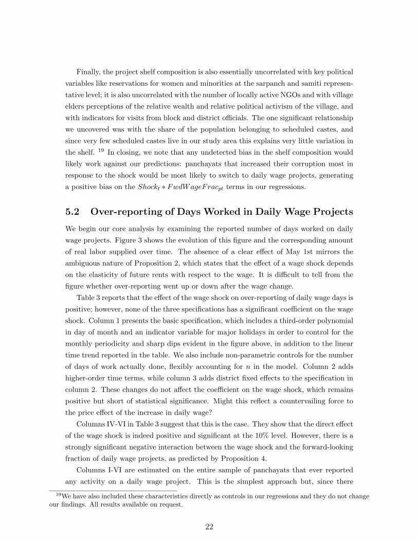
5.2 Over-reporting of Days Worked in Daily Wage Projects
We begin our core analysis by examining the reported number of days worked on daily
wage projects. Figure 3 shows the evolution of this figure and the corresponding amount
of real labor supplied over time. The absence of a clear effect of May 1st mirrors the
ambiguous nature of Proposition 2, which states that the effect of a wage shock depends
on the elasticity of future rents with respect to the wage. It is difficult to tell from the
figure whether over-reporting went up or down after the wage change.
Table 3 reports that the effect of the wage shock on over-reporting of daily wage days is
positive; however, none of the three specifications has a significant coefficient on the wage
shock. Column 1 presents the basic specification, which includes a third-order polynomial
in day of month and an indicator variable for major holidays in order to control for the
monthly periodicity and sharp dips evident in the figure above, in addition to the linear
time trend reported in the table. We also include non-parametric controls for the number
of days of work actually done, flexibly accounting for n in the model. Column 2 adds
higher-order time terms, while column 3 adds district fixed effects to the specification in
column 2. These changes do not affect the coefficient on the wage shock, which remains
positive but short of statistical significance. Might this reflect a countervailing force to
the price effect of the increase in daily wage?
Columns IV-VI in Table 3 suggest that this is the case. They show that the direct effect
of the wage shock is indeed positive and significant at the 10% level. However, there is a
strongly significant negative interaction between the wage shock and the forward-looking
fraction of daily wage projects, as predicted by Proposition 4.
Columns I-VI are estimated on the entire sample of panchayats that ever reported
any activity on a daily wage project. This is the simplest approach but, since there
19We have also included these characteristics directly as controls in our regressions and they do not changeour findings. All results available on request.
22
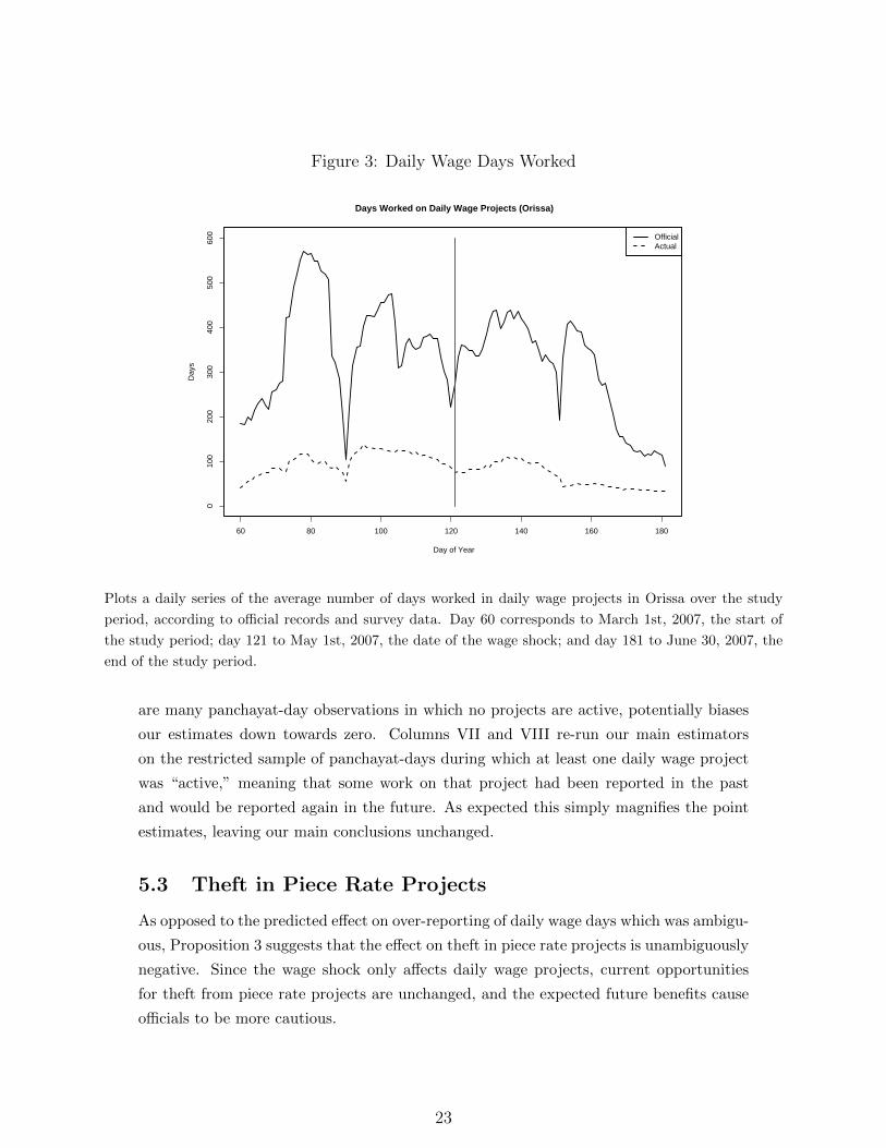
Figure 3: Daily Wage Days Worked
60 80 100 120 140 160 180
010
020
030
040
050
060
0
Day of Year
Day
s
Days Worked on Daily Wage Projects (Orissa)
OfficialActual
Plots a daily series of the average number of days worked in daily wage projects in Orissa over the study
period, according to official records and survey data. Day 60 corresponds to March 1st, 2007, the start of
the study period; day 121 to May 1st, 2007, the date of the wage shock; and day 181 to June 30, 2007, the
end of the study period.
are many panchayat-day observations in which no projects are active, potentially biases
our estimates down towards zero. Columns VII and VIII re-run our main estimators
on the restricted sample of panchayat-days during which at least one daily wage project
was “active,” meaning that some work on that project had been reported in the past
and would be reported again in the future. As expected this simply magnifies the point
estimates, leaving our main conclusions unchanged.
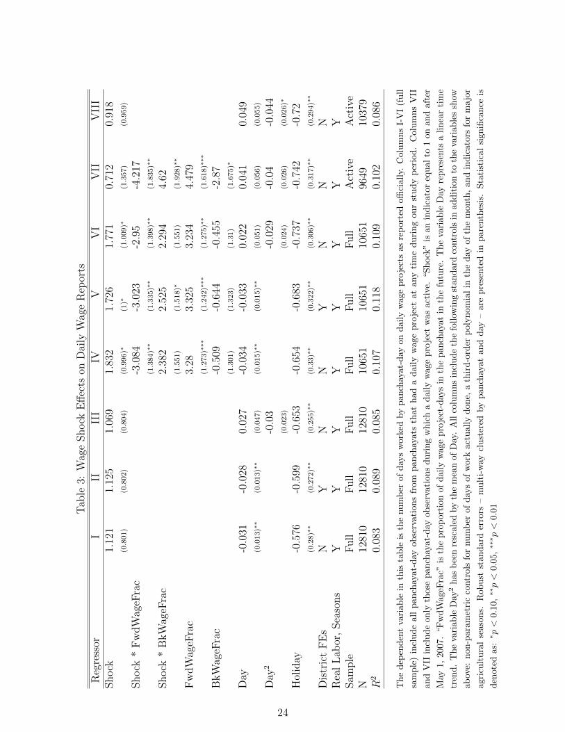
5.3 Theft in Piece Rate Projects
As opposed to the predicted effect on over-reporting of daily wage days which was ambigu-
ous, Proposition 3 suggests that the effect on theft in piece rate projects is unambiguously
negative. Since the wage shock only affects daily wage projects, current opportunities
for theft from piece rate projects are unchanged, and the expected future benefits cause
officials to be more cautious.
23
Tab
le3:
Wag
eShock
Eff
ects
onD
aily
Wag
eR
epor
ts
Reg
ress
orI
IIII
IIV
VV
IV
IIV
III
Shock
1.12
11.
125
1.06
91.
832
1.72
61.
771
0.71
20.
918
(0.8
01)
(0.8
02)
(0.8
04)
(0.9
96)∗
(1)∗
(1.0
09)∗
(1.3
57)
(0.9
59)
Shock
*F
wdW
ageF
rac
-3.0
84-3
.023
-2.9
5-4
.217
(1.3
84)∗∗
(1.3
35)∗∗
(1.3
98)∗∗
(1.8
35)∗∗
Shock
*B
kW
ageF
rac
2.38
22.
525
2.29
44.
62(1
.551)
(1.5
18)∗
(1.5
51)
(1.9
28)∗∗
Fw
dW
ageF
rac
3.28
3.32
53.
234
4.47
9(1
.273)∗∗∗
(1.2
42)∗∗∗
(1.2
75)∗∗
(1.6
18)∗∗∗
BkW
ageF
rac
-0.5
09-0
.644
-0.4
55-2
.87
(1.3
01)
(1.3
23)
(1.3
1)
(1.6
75)∗
Day
-0.0
31-0
.028
0.02
7-0
.034
-0.0
330.
022
0.04
10.
049
(0.0
13)∗∗
(0.0
13)∗∗
(0.0
47)
(0.0
15)∗∗
(0.0
15)∗∗
(0.0
51)
(0.0
56)
(0.0
55)
Day
2-0
.03
-0.0
29-0
.04
-0.0
44(0
.023)
(0.0
24)
(0.0
26)
(0.0
26)∗
Hol
iday
-0.5
76-0
.599
-0.6
53-0
.654
-0.6
83-0
.737
-0.7
42-0
.72
(0.2
8)∗∗
(0.2
72)∗∗
(0.2
55)∗∗
(0.3
3)∗∗
(0.3
22)∗∗
(0.3
06)∗∗
(0.3
17)∗∗
(0.2
94)∗∗
Dis
tric
tF
Es
NY
NN
YN
NN
Rea
lL
abor
,Sea
sons
YY
YY
YY
YY
Sam
ple
Full
Full
Full
Full
Full
Full
Act
ive
Act
ive
N12
810
1281
012
810
1065
110
651
1065
196
4910
379
R2
0.08
30.
089
0.08
50.
107
0.11
80.
109
0.10
20.
086
Th
ed
epen
den
tva
riab
lein
this
tab
leis
the
nu
mb
erof
day
sw
ork
edby
pan
chay
at-
day
on
dail
yw
age
pro
ject
sas
rep
ort
edoffi
ciall
y.C
olu
mn
sI-
VI
(fu
ll
sam
ple
)in
clud
eal
lp
anch
ayat
-day
obse
rvat
ion
sfr
omp
an
chay
ats
that
had
ad
ail
yw
age
pro
ject
at
any
tim
ed
uri
ng
ou
rst
ud
yp
erio
d.
Colu
mn
sV
II
and
VII
incl
ud
eon
lyth
ose
pan
chay
at-d
ayob
serv
atio
ns
du
rin
gw
hic
ha
dail
yw
age
pro
ject
was
act
ive.
“S
hock
”is
an
ind
icato
req
ual
to1
on
an
daft
er
May
1,20
07.
“Fw
dW
ageF
rac”
isth
ep
rop
orti
onof
dail
yw
age
pro
ject
-day
sin
the
pan
chay
at
inth
efu
ture
.T
he
vari
ab
leD
ayre
pre
sents
alin
ear
tim
e
tren
d.
Th
eva
riab
leD
ay2
has
bee
nre
scal
edby
the
mea
nof
Day
.A
llco
lum
ns
incl
ud
eth
efo
llow
ing
stan
dard
contr
ols
inad
dit
ion
toth
eva
riab
les
show
abov
e:n
on-p
aram
etri
cco
ntr
ols
for
nu
mb
erof
day
sof
work
act
uall
yd
on
e,a
thir
d-o
rder
poly
nom
ial
inth
ed
ayof
the
month
,an
din
dic
ato
rsfo
rm
ajo
r
agri
cult
ura
lse
ason
s.R
obu
stst
and
ard
erro
rs–
mu
lti-
way
clu
ster
edby
pan
chay
at
an
dd
ay–
are
pre
sente
din
pare
nth
esis
.S
tati
stic
al
sign
ifica
nce
is
den
oted
as:∗ p<
0.10
,∗∗p<
0.0
5,∗∗∗ p<
0.01
24
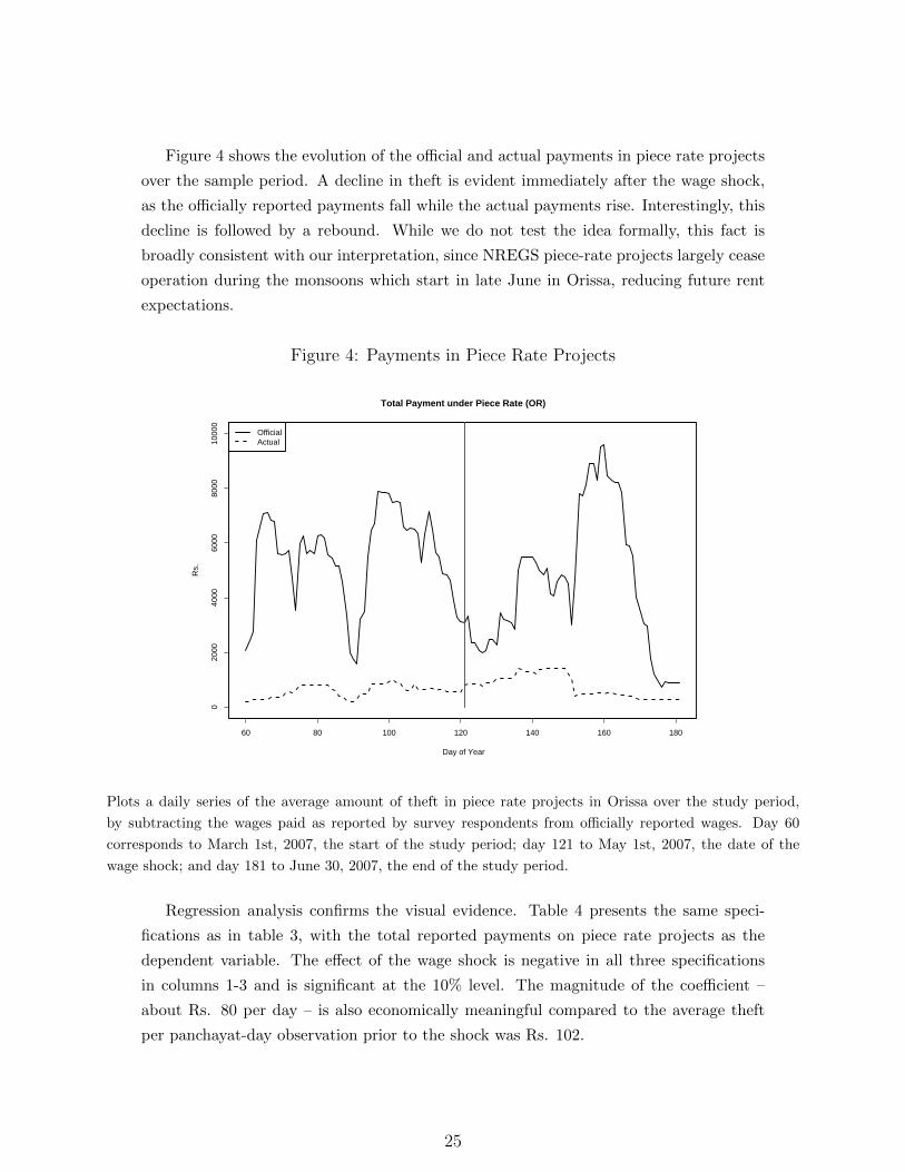
Figure 4 shows the evolution of the official and actual payments in piece rate projects
over the sample period. A decline in theft is evident immediately after the wage shock,
as the officially reported payments fall while the actual payments rise. Interestingly, this
decline is followed by a rebound. While we do not test the idea formally, this fact is
broadly consistent with our interpretation, since NREGS piece-rate projects largely cease
operation during the monsoons which start in late June in Orissa, reducing future rent
expectations.
Figure 4: Payments in Piece Rate Projects
60 80 100 120 140 160 180
020
0040
0060
0080
0010
000
Day of Year
Rs.
OfficialActual
Total Payment under Piece Rate (OR)
Plots a daily series of the average amount of theft in piece rate projects in Orissa over the study period,
by subtracting the wages paid as reported by survey respondents from officially reported wages. Day 60
corresponds to March 1st, 2007, the start of the study period; day 121 to May 1st, 2007, the date of the
wage shock; and day 181 to June 30, 2007, the end of the study period.
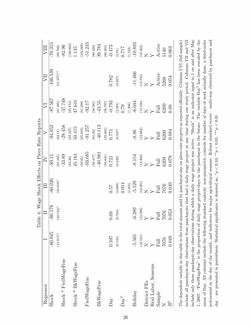
Regression analysis confirms the visual evidence. Table 4 presents the same speci-
fications as in table 3, with the total reported payments on piece rate projects as the
dependent variable. The effect of the wage shock is negative in all three specifications
in columns 1-3 and is significant at the 10% level. The magnitude of the coefficient –
about Rs. 80 per day – is also economically meaningful compared to the average theft
per panchayat-day observation prior to the shock was Rs. 102.
25
Tab
le4:
Wag
eShock
Eff
ects
onP
iece
Rat
eR
epor
ts
Reg
ress
orI
IIII
IIV
VV
IV
IIV
III
Shock
-80.
045
-80.
578
-80.
026
-89.
11-9
4.05
2-8
7.56
7-1
00.5
39-7
0.31
5(4
1.9
17)∗
(42.1
34)∗
(42.0
18)∗
(61.2
45)
(62.1
1)
(61.4
95)
(51.2
77)∗∗
(69.7
06)
Shock
*F
wdW
ageF
rac
-33.
89-2
8.45
8-3
7.74
8-8
2.96
(93.3
6)
(93.1
97)
(95.8
72)
(126.9
02)
Shock
*B
kW
ageF
rac
45.1
6150
.415
47.6
411.
145
(59.8
5)
(65.0
43)
(61.2
98)
(102.0
69)
Fw
dW
ageF
rac
-93.
685
-91.
257
-92.
17-5
1.23
3(5
8.4
17)
(61.9
2)
(58.5
81)
(80.3
26)
BkW
ageF
rac
-40.
981
-40.
113
-43.
5539
.784
(56.8
31)
(59.8
65)
(56.7
97)
(90.3
04)
Day
0.59
70.
690.
570.
721
0.77
1-0
.793
0.78
2-0
.473
(0.7
45)
(0.7
64)
(2.0
09)
(0.8
49)
(0.8
47)
(2.3
81)
(0.8
57)
(2.9
1)
Day
20.
014
0.79
0.71
7(1
.055)
(1.3
08)
(1.5
23)
Hol
iday
-5.5
65-6
.289
-5.5
29-8
.154
-8.8
6-6
.044
-11.
466
-10.
893
(12.5
21)
(12.5
98)
(12.2
81)
(13.4
63)
(13.6
62)
(14.1
56)
(14.7
24)
(16.3
03)
Dis
tric
tF
Es
NY
NN
YN
NN
Rea
lL
abor
,Sea
sons
YY
YY
YY
YY
Sam
ple
Full
Full
Full
Full
Full
Full
Act
ive
Act
ive
N70
7670
7670
7662
0962
0962
0952
6851
40R
20.
049
0.05
30.
049
0.07
90.
084
0.08
0.05
40.
063
Th
ed
epen
den
tva
riab
lein
this
tab
leis
the
tota
lam
ount
paid
by
pan
chay
at-
day
on
pie
ce-r
ate
pro
ject
sas
rep
ort
edoffi
ciall
y.C
olu
mns
I-V
I(f
ull
sam
ple
)
incl
ud
eal
lp
anch
ayat
-day
obse
rvat
ion
sfr
omp
anch
ayats
that
had
ad
ail
yw
age
pro
ject
at
any
tim
ed
uri
ng
ou
rst
ud
yp
erio
d.
Colu
mn
sV
IIan
dV
II
incl
ud
eon
lyth
ose
pan
chay
at-d
ayob
serv
atio
ns
du
rin
gw
hic
ha
dail
yw
age
pro
ject
was
act
ive.
“S
hock
”is
an
ind
icato
req
ual
to1
on
an
daft
erM
ay
1,20
07.
“Fw
dW
ageF
rac”
isth
ep
rop
orti
onof
dai
lyw
age
pro
ject
-day
sin
the
pan
chay
at
inth
efu
ture
.T
he
vari
ab
leD
ay2
has
bee
nre
scale
dby
the
mea
nof
Day
.A
llco
lum
ns
incl
ud
eth
efo
llow
ing
stan
dard
contr
ols
:non
-para
met
ric
contr
ols
for
nu
mb
erof
day
sof
work
act
uall
yd
on
e,a
thir
d-o
rder
pol
yn
omia
lin
the
day
ofth
em
onth
,an
din
dic
ator
sfo
rm
ajo
ragri
cult
ura
lse
aso
ns.
Rob
ust
stan
dard
erro
rs–
mu
lti-
way
clu
ster
edby
pan
chay
at
an
d
day
–ar
ep
rese
nte
din
par
enth
esis
.S
tati
stic
alsi
gnifi
can
ceis
den
ote
das:∗ p<
0.1
0,∗∗p<
0.05,∗∗∗ p<
0.0
1
26
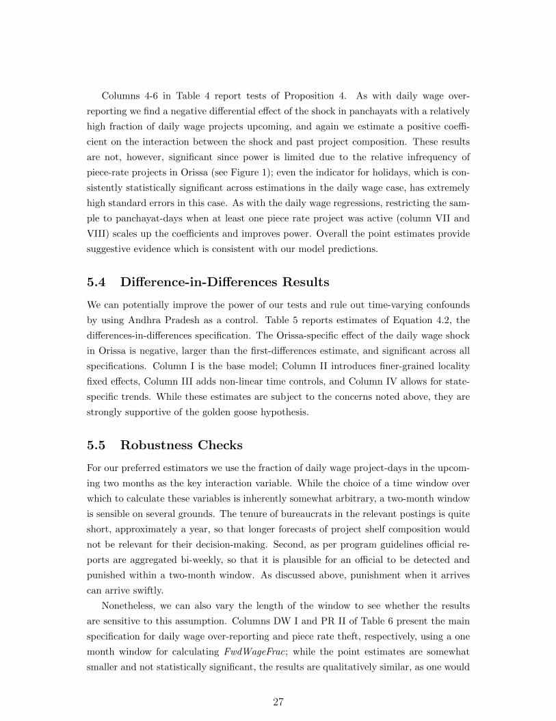
Columns 4-6 in Table 4 report tests of Proposition 4. As with daily wage over-
reporting we find a negative differential effect of the shock in panchayats with a relatively
high fraction of daily wage projects upcoming, and again we estimate a positive coeffi-
cient on the interaction between the shock and past project composition. These results
are not, however, significant since power is limited due to the relative infrequency of
piece-rate projects in Orissa (see Figure 1); even the indicator for holidays, which is con-
sistently statistically significant across estimations in the daily wage case, has extremely
high standard errors in this case. As with the daily wage regressions, restricting the sam-
ple to panchayat-days when at least one piece rate project was active (column VII and
VIII) scales up the coefficients and improves power. Overall the point estimates provide
suggestive evidence which is consistent with our model predictions.
5.4 Difference-in-Differences Results
We can potentially improve the power of our tests and rule out time-varying confounds
by using Andhra Pradesh as a control. Table 5 reports estimates of Equation 4.2, the
differences-in-differences specification. The Orissa-specific effect of the daily wage shock
in Orissa is negative, larger than the first-differences estimate, and significant across all
specifications. Column I is the base model; Column II introduces finer-grained locality
fixed effects, Column III adds non-linear time controls, and Column IV allows for state-
specific trends. While these estimates are subject to the concerns noted above, they are
strongly supportive of the golden goose hypothesis.
5.5 Robustness Checks
For our preferred estimators we use the fraction of daily wage project-days in the upcom-
ing two months as the key interaction variable. While the choice of a time window over
which to calculate these variables is inherently somewhat arbitrary, a two-month window
is sensible on several grounds. The tenure of bureaucrats in the relevant postings is quite
short, approximately a year, so that longer forecasts of project shelf composition would
not be relevant for their decision-making. Second, as per program guidelines official re-
ports are aggregated bi-weekly, so that it is plausible for an official to be detected and
punished within a two-month window. As discussed above, punishment when it arrives
can arrive swiftly.
Nonetheless, we can also vary the length of the window to see whether the results
are sensitive to this assumption. Columns DW I and PR II of Table 6 present the main
specification for daily wage over-reporting and piece rate theft, respectively, using a one
month window for calculating FwdWageFrac; while the point estimates are somewhat
smaller and not statistically significant, the results are qualitatively similar, as one would
27
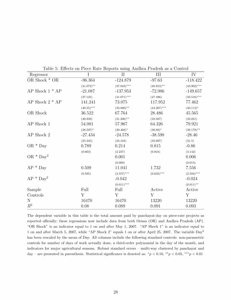
Table 5: Effects on Piece Rate Reports using Andhra Pradesh as a Control
Regressor I II III IVOR Shock * OR -96.364 -124.879 -97.63 -118.422
(41.073)∗∗ (37.843)∗∗∗ (48.853)∗∗ (43.902)∗∗∗
AP Shock 1 * AP -21.087 -137.953 -72.986 -149.657(37.125) (41.071)∗∗∗ (47.496) (50.516)∗∗∗
AP Shock 2 * AP 141.241 73.075 117.952 77.462(40.55)∗∗∗ (33.886)∗∗ (44.267)∗∗∗ (40.113)∗
OR Shock 36.522 67.764 28.486 45.565(30.939) (31.206)∗∗ (32.507) (32.051)
AP Shock 1 54.081 57.967 64.326 79.921(28.597)∗ (30.468)∗ (38.09)∗ (39.178)∗∗
AP Shock 2 -27.434 -24.578 -38.598 -28.46(25.345) (24.104) (33.807) (31.5)
OR * Day 0.789 0.214 0.815 -0.86(0.663) (2.237) (0.824) (3.142)
OR * Day2 0.001 0.006(0.009) (0.013)
AP * Day 0.509 11.041 1.732 7.556(0.595) (2.557)∗∗∗ (0.632)∗∗∗ (2.594)∗∗∗
AP * Day2 -0.042 -0.024(0.011)∗∗∗ (0.011)∗∗
Sample Full Full Active ActiveControls Y Y Y YN 16470 16470 13220 13220R2 0.08 0.089 0.091 0.093
The dependent variable in this table is the total amount paid by panchayat-day on piece-rate projects as
reported officially; these regressions now include data from both Orissa (OR) and Andhra Pradesh (AP).
“OR Shock” is an indicator equal to 1 on and after May 1, 2007. “AP Shock 1” is an indicator equal to
1 on and after March 5, 2007, while “AP Shock 2” equals 1 on or after April 25, 2007. The variable Day2
has been rescaled by the mean of Day. All columns include the following standard controls: non-parametric
controls for number of days of work actually done, a third-order polynomial in the day of the month, and
indicators for major agricultural seasons. Robust standard errors – multi-way clustered by panchayat and
day – are presented in parenthesis. Statistical significance is denoted as: ∗p < 0.10, ∗∗p < 0.05, ∗∗∗p < 0.01
28
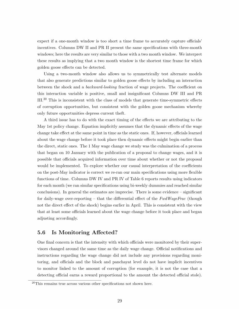
expect if a one-month window is too short a time frame to accurately capture officials’
incentives. Columns DW II and PR II present the same specifications with three-month
windows; here the results are very similar to those with a two month window. We interpret
these results as implying that a two month window is the shortest time frame for which
golden goose effects can be detected.
Using a two-month window also allows us to symmetrically test alternate models
that also generate predictions similar to golden goose effects by including an interaction
between the shock and a backward-looking fraction of wage projects. The coefficient on
this interaction variable is positive, small and insignificant Columns DW III and PR
III.20 This is inconsistent with the class of models that generate time-symmetric effects
of corruption opportunities, but consistent with the golden goose mechanism whereby
only future opportunities depress current theft.
A third issue has to do with the exact timing of the effects we are attributing to the
May 1st policy change. Equation implicitly assumes that the dynamic effects of the wage
change take effect at the same point in time as the static ones. If, however, officials learned
about the wage change before it took place then dynamic effects might begin earlier than
the direct, static ones. The 1 May wage change we study was the culmination of a process
that began on 10 January with the publication of a proposal to change wages, and it is
possible that officials acquired information over time about whether or not the proposal
would be implemented. To explore whether our causal interpretation of the coefficients
on the post-May indicator is correct we re-ran our main specifications using more flexible
functions of time. Columns DW IV and PR IV of Table 6 reports results using indicators
for each month (we ran similar specifications using bi-weekly dummies and reached similar
conclusions). In general the estimates are imprecise. There is some evidence – significant
for daily-wage over-reporting – that the differential effect of the FwdWageFrac (though
not the direct effect of the shock) begins earlier in April. This is consistent with the view
that at least some officials learned about the wage change before it took place and began
adjusting accordingly.
5.6 Is Monitoring Affected?
One final concern is that the intensity with which officials were monitored by their super-
visors changed around the same time as the daily wage change. Official notifications and
instructions regarding the wage change did not include any provisions regarding moni-
toring, and officials and the block and panchayat level do not have implicit incentives
to monitor linked to the amount of corruption (for example, it is not the case that a
detecting official earns a reward proportional to the amount the detected official stole).
20This remains true across various other specifications not shown here.
29
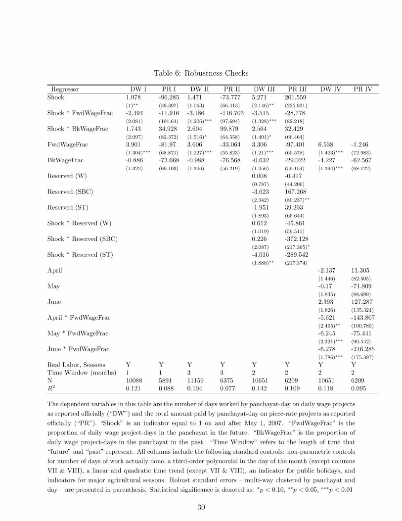
Table 6: Robustness Checks
Regressor DW I PR I DW II PR II DW III PR III DW IV PR IVShock 1.978 -96.285 1.471 -73.777 5.271 201.559
(1)∗∗ (59.397) (1.063) (66.413) (2.146)∗∗ (225.931)
Shock * FwdWageFrac -2.494 -11.916 -3.186 -116.703 -3.515 -28.778(2.081) (101.64) (1.206)∗∗∗ (97.694) (1.328)∗∗∗ (82.218)
Shock * BkWageFrac 1.743 34.928 2.604 99.879 2.564 32.429(2.097) (82.372) (1.516)∗ (64.558) (1.401)∗ (66.464)
FwdWageFrac 3.901 -81.97 3.606 -33.064 3.306 -97.401 6.538 -1.246(1.304)∗∗∗ (68.871) (1.227)∗∗∗ (55.823) (1.21)∗∗∗ (60.578) (1.403)∗∗∗ (72.983)
BkWageFrac -0.886 -73.668 -0.988 -76.568 -0.632 -29.022 -4.227 -62.567(1.322) (69.103) (1.306) (56.219) (1.256) (59.154) (1.394)∗∗∗ (68.122)
Reserved (W) 0.008 -0.417(0.787) (44.206)
Reserved (SBC) -3.623 167.268(2.342) (80.237)∗∗
Reserved (ST) -1.951 39.203(1.893) (65.644)
Shock * Reserved (W) 0.612 -45.861(1.019) (59.511)
Shock * Reserved (SBC) 0.226 -372.128(2.087) (217.365)∗
Shock * Reserved (ST) -4.016 -289.542(1.888)∗∗ (217.374)
April -2.137 11.305(1.446) (82.505)
May -0.17 -71.809(1.835) (88.699)
June 2.393 127.287(1.826) (135.324)
April * FwdWageFrac -5.621 -143.807(2.465)∗∗ (100.789)
May * FwdWageFrac -6.245 -75.441(2.321)∗∗∗ (90.542)
June * FwdWageFrac -6.278 -216.285(1.786)∗∗∗ (175.397)
Real Labor, Seasons Y Y Y Y Y Y Y YTime Window (months) 1 1 3 3 2 2 2 2N 10088 5891 11159 6375 10651 6209 10651 6209R2 0.121 0.088 0.104 0.077 0.142 0.109 0.118 0.095
The dependent variables in this table are the number of days worked by panchayat-day on daily wage projects
as reported officially (“DW”) and the total amount paid by panchayat-day on piece-rate projects as reported
officially (“PR”). “Shock” is an indicator equal to 1 on and after May 1, 2007. “FwdWageFrac” is the
proportion of daily wage project-days in the panchayat in the future. “BkWageFrac” is the proportion of
daily wage project-days in the panchayat in the past. “Time Window” refers to the length of time that
“future” and “past” represent. All columns include the following standard controls: non-parametric controls
for number of days of work actually done, a third-order polynomial in the day of the month (except columns
VII & VIII), a linear and quadratic time trend (except VII & VIII), an indicator for public holidays, and
indicators for major agricultural seasons. Robust standard errors – multi-way clustered by panchayat and
day – are presented in parenthesis. Statistical significance is denoted as: ∗p < 0.10, ∗∗p < 0.05, ∗∗∗p < 0.01
30
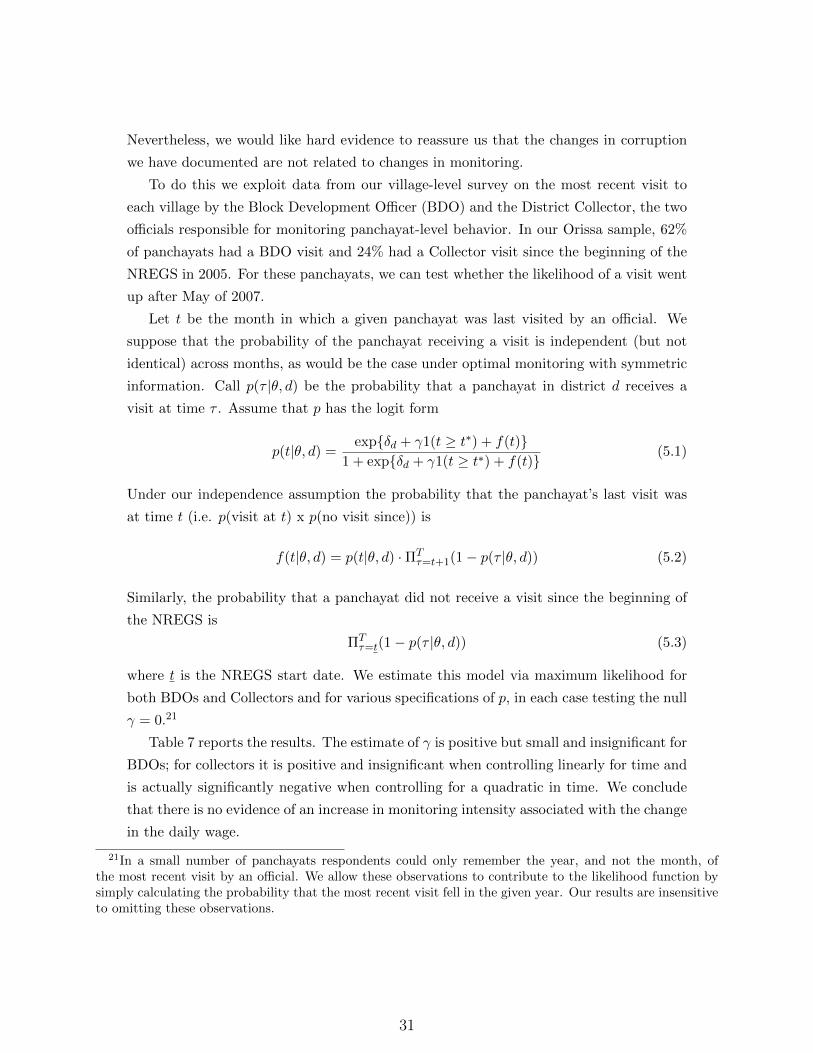
Nevertheless, we would like hard evidence to reassure us that the changes in corruption
we have documented are not related to changes in monitoring.
To do this we exploit data from our village-level survey on the most recent visit to
each village by the Block Development Officer (BDO) and the District Collector, the two
officials responsible for monitoring panchayat-level behavior. In our Orissa sample, 62%
of panchayats had a BDO visit and 24% had a Collector visit since the beginning of the
NREGS in 2005. For these panchayats, we can test whether the likelihood of a visit went
up after May of 2007.
Let t be the month in which a given panchayat was last visited by an official. We
suppose that the probability of the panchayat receiving a visit is independent (but not
identical) across months, as would be the case under optimal monitoring with symmetric
information. Call p(τ |θ, d) be the probability that a panchayat in district d receives a
visit at time τ . Assume that p has the logit form
p(t|θ, d) =exp{δd + γ1(t ≥ t∗) + f(t)}
1 + exp{δd + γ1(t ≥ t∗) + f(t)}(5.1)
Under our independence assumption the probability that the panchayat’s last visit was
at time t (i.e. p(visit at t) x p(no visit since)) is
f(t|θ, d) = p(t|θ, d) ·ΠTτ=t+1(1− p(τ |θ, d)) (5.2)
Similarly, the probability that a panchayat did not receive a visit since the beginning of
the NREGS is
ΠTτ=t(1− p(τ |θ, d)) (5.3)
where t is the NREGS start date. We estimate this model via maximum likelihood for
both BDOs and Collectors and for various specifications of p, in each case testing the null
γ = 0.21
Table 7 reports the results. The estimate of γ is positive but small and insignificant for
BDOs; for collectors it is positive and insignificant when controlling linearly for time and
is actually significantly negative when controlling for a quadratic in time. We conclude
that there is no evidence of an increase in monitoring intensity associated with the change
in the daily wage.
21In a small number of panchayats respondents could only remember the year, and not the month, ofthe most recent visit by an official. We allow these observations to contribute to the likelihood function bysimply calculating the probability that the most recent visit fell in the given year. Our results are insensitiveto omitting these observations.
31
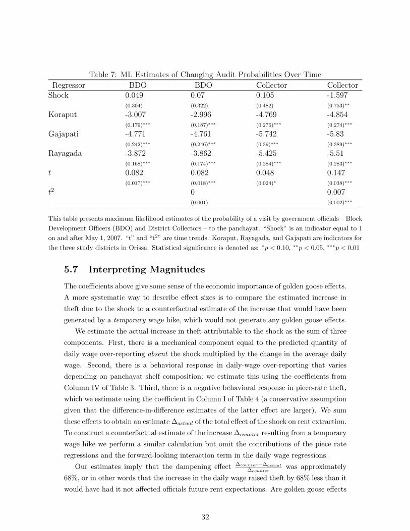
Table 7: ML Estimates of Changing Audit Probabilities Over Time
Regressor BDO BDO Collector CollectorShock 0.049 0.07 0.105 -1.597
(0.304) (0.322) (0.482) (0.753)∗∗
Koraput -3.007 -2.996 -4.769 -4.854(0.179)∗∗∗ (0.187)∗∗∗ (0.276)∗∗∗ (0.274)∗∗∗
Gajapati -4.771 -4.761 -5.742 -5.83(0.242)∗∗∗ (0.246)∗∗∗ (0.39)∗∗∗ (0.389)∗∗∗
Rayagada -3.872 -3.862 -5.425 -5.51(0.168)∗∗∗ (0.174)∗∗∗ (0.284)∗∗∗ (0.283)∗∗∗
t 0.082 0.082 0.048 0.147(0.017)∗∗∗ (0.018)∗∗∗ (0.024)∗ (0.038)∗∗∗
t2 0 0.007(0.001) (0.002)∗∗∗
This table presents maximum likelihood estimates of the probability of a visit by government officials – Block
Development Officers (BDO) and District Collectors – to the panchayat. “Shock” is an indicator equal to 1
on and after May 1, 2007. “t” and “t2” are time trends. Koraput, Rayagada, and Gajapati are indicators for
the three study districts in Orissa. Statistical significance is denoted as: ∗p < 0.10, ∗∗p < 0.05, ∗∗∗p < 0.01
5.7 Interpreting Magnitudes
The coefficients above give some sense of the economic importance of golden goose effects.
A more systematic way to describe effect sizes is to compare the estimated increase in
theft due to the shock to a counterfactual estimate of the increase that would have been
generated by a temporary wage hike, which would not generate any golden goose effects.
We estimate the actual increase in theft attributable to the shock as the sum of three
components. First, there is a mechanical component equal to the predicted quantity of
daily wage over-reporting absent the shock multiplied by the change in the average daily
wage. Second, there is a behavioral response in daily-wage over-reporting that varies
depending on panchayat shelf composition; we estimate this using the coefficients from
Column IV of Table 3. Third, there is a negative behavioral response in piece-rate theft,
which we estimate using the coefficient in Column I of Table 4 (a conservative assumption
given that the difference-in-difference estimates of the latter effect are larger). We sum
these effects to obtain an estimate ∆actual of the total effect of the shock on rent extraction.
To construct a counterfactual estimate of the increase ∆counter resulting from a temporary
wage hike we perform a similar calculation but omit the contributions of the piece rate
regressions and the forward-looking interaction term in the daily wage regressions.
Our estimates imply that the dampening effect ∆counter−∆actual∆counter
was approximately
68%, or in other words that the increase in the daily wage raised theft by 68% less than it
would have had it not affected officials future rent expectations. Are golden goose effects
32
of this magnitude plausible? Direct calibration of our model is not possible without data
on all the sources of rent which a corrupt official would lose if suspended or fired. In
principle, large golden goose effects are likely precisely where rent extraction is high due
to weak monitoring. When the chance of detection is low, future rents not only become
large but become very sensitive to changes in the likelihood of detection. Intuitively,
weak monitoring lengthens the effective time horizon, increasing the sensitivity of rents
to a daily wage change and thus magnifying golden goose effects.22
6 Conclusion
Dismissal, suspension, and transfer are standard tools for disciplining corrupt agents. We
show that these incentives generate a “golden goose” effect: as steady-state opportunities
to extract rent increase the value of continuing in office increases and this induces agents
to act more cautiously. This dynamic mechanism tends to dampen, and may reverse, the
predictions of static models.
We test for golden goose effects using panel data on corruption in India’s National
Rural Employment Guarantee Scheme, exploiting an exogenous increase in program wages
to construct tests. We find two forms of evidence consistent with our theory: higher daily
wages lead to lower theft from piece rate projects, and differentially lower theft in areas
with a higher proportion of daily wage projects upcoming. Rough calculations based on
the point estimates imply that these effects reduced the increase in corruption generated
by the wage change by approximately 68%.
22As an illustration, if a perfectly patient (β = 1) official only supervises wage projects (φ = 1) andover-reports a fixed number n̂ − n of days per period, then the sensitivity of his continuation value to thedaily wage
∂V
∂w=
n̂− nπ(n̂, n)
(5.4)
becomes very large as the probability of detection π falls.
33
References
Acemoglu, Daron and Thierry Verdier, “The Choice between Market Failures and
Corruption,” American Economic Review, March 2000, 90 (1), 194–211.
Ahlin, Christian, “Effects and (In)tractability of Decentralized Corruption,” mimeo,
Vanderbilt University December 2005.
Andvig, Jens Chr. and Karl Ove Moene, “How corruption may corrupt,” Journal
of Economic Behavior & Organization, January 1990, 13 (1), 63–76.
Banerjee, Abhijit V, “A Theory of Misgovernance,” The Quarterly Journal of Eco-
nomics, November 1997, 112 (4), 1289–1332.
Barro, Robert, “The Control of Politicians, an Economic Model,” Public Choice, March
1973, 14 (1), 19–42.
Becker, Gary S. and George J. Stigler, “Law Enforcement, Malfeasance, and Com-
pensation of Enforcers,” The Journal of Legal Studies, 1974, 3 (1), 1–18.
Bertrand, Marianne, Simeon Djankov, Rema Hanna, and Sendhil Mul-
lainathan, “Obtaining a Driver’s License in India: An Experimental Approach to
Studying Corruption,” The Quarterly Journal of Economics, November 2007, 122
(4), 1639–1676.
Besley, Timothy and John McLaren, “Taxes and Bribery: The Role of Wage Incen-
tives,” Economic Journal, January 1993, 103 (416), 119–41.
Cadot, Olivier, “Corruption as a gamble,” Journal of Public Economics, July 1987, 33
(2), 223–244.
Chattopadhyay, Raghabendra and Esther Duflo, “Women as Policy Makers: Evi-
dence from a Randomized Policy Experiment in India,” Econometrica, 09 2004, 72
(5), 1409–1443.
Das, S.K., Public Office, Private Interest: Bureaucracy and Corruption in India, New
Delhi: Oxford University Press, 2001.
de Zwart, Frank, The Bureaucratic Merry-Go-Round, Amsterdam: Amsterdam Uni-
versity Press, 1994.
Ferejohn, John, “Incumbent performance and electoral control,” Public Choice, Jan-
uary 1986, 50 (1-3), 5–25.
Ferraz, Claudio and Frederico Finan, “Exposing Corrupt Politicians: The Effects of
Brazil’s Publicly Released Audits on Electoral Outcomes,” The Quarterly Journal
of Economics, 05 2008, 123 (2), 703–745.
34
and , “Electoral Accountability and Corruption: Evidence from the Audits of
Local Governments,” NBER Working Papers 14937, National Bureau of Economic
Research, Inc April 2009.
Huntington, Samuel, “Modernisation and Corruption,” in “Political Order in Changing
Societies,” New Haven: Yale University Press, 1968.
Iyer, Lakshmi and Anandi Mani, “Traveling Agents: Political Change and Bureau-
cratic Turnover in India,” Working Paper 09-006, Harvard Business School 2009.
Leff, Nathaniel, “Economic Development through Bureaucratic Corruption,” American
Behavioural Scientist, 1964, 8, 8–14.
McMillan, Margaret, “Why Kill The Golden Goose? A Political-Economy Model Of
Export Taxation,” The Review of Economics and Statistics, February 2001, 83 (1),
170–184.
Ministry of Law and Justice, “The National Rural Employment Guarantee Act,
2005,” The Gazette of India, September 2005.
Ministry of Rural Development, The National Rural Employment Guarantee Act
2005: Operation Guidelines 2008, 3rd ed. 2008.
Mookherjee, Dilip and I P L Png, “Corruptible Law Enforcers: How Should They
Be Compensated?,” Economic Journal, January 1995, 105 (428), 145–59.
Nagin, Daniel S., James B. Rebitzer, Seth Sanders, and Lowell J. Taylor,
“Monitoring, Motivation, and Management: The Determinants of Opportunistic
Behavior in a Field Experiment,” American Economic Review, September 2002, 92
(4), 850–873.
Niehaus, Paul and Sandip Sukhtankar, “Marginal Leakage in Public Programs,”
Technical Report, Dartmouth College 2010.
Olken, Benjamin A., “Corruption and the costs of redistribution: Micro evidence from
Indonesia,” Journal of Public Economics, May 2006, 90 (4-5), 853–870.
, “Monitoring Corruption: Evidence from a Field Experiment in Indonesia,” Journal
of Political Economy, April 2007, 115 (2), 200–249.
, “Corruption perceptions vs. corruption reality,” Journal of Public Economics, Au-
gust 2009, 93 (7-8), 950–964.
Olson, Mancur, Power and Prosperity: Outgrowing Communist and Capitalist Dicta-
torships, New York: Basic Books, 2000.
Persson, Torsten, Gerard Roland, and Guido Tabellini, “Separation of Powers
and Political Accountability,” The Quarterly Journal of Economics, November 1997,
112 (4), 1163–1202.
35
Reinikka, Ritva and Jakob Svensson, “Local Capture: Evidence From a Central
Government Transfer Program in Uganda,” The Quarterly Journal of Economics,
May 2004, 119 (2), 678–704.
and , “Fighting Corruption to Improve Schooling: Evidence from a Newspaper
Campaign in Uganda,” Journal of the European Economic Association, 04/05 2005,
3 (2-3), 259–267.
Shleifer, Andrei and Robert W Vishny, “Corruption,” The Quarterly Journal of
Economics, August 1993, 108 (3), 599–617.
Tella, Rafael Di and Ernesto Schargrodsky, “The Role of Wages and Auditing
during a Crackdown on Corruption in the City of Buenos Aires,” Journal of Law &
Economics, April 2003, 46 (1), 269–92.
Yang, Dean, “Can Enforcement Backfire? Crime Displacement in the Context of Cus-
toms Reform in the Philippines,” The Review of Economics and Statistics, November
2008, 90 (1), 1–14.
36
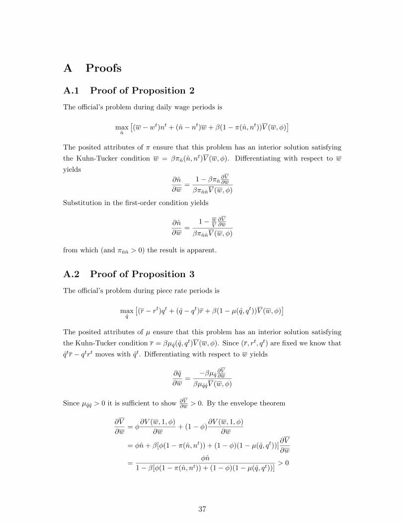
A Proofs
A.1 Proof of Proposition 2
The official’s problem during daily wage periods is
maxn̂
[(w − wt)nt + (n̂− nt)w + β(1− π(n̂, nt))V (w, φ)
]The posited attributes of π ensure that this problem has an interior solution satisfying
the Kuhn-Tucker condition w = βπn̂(n̂, nt)V (w, φ). Differentiating with respect to w
yields
∂n̂
∂w=
1− βπn̂ ∂V∂wβπn̂n̂V (w, φ)
Substitution in the first-order condition yields
∂n̂
∂w=
1− wV∂V∂w
βπn̂n̂V (w, φ)
from which (and πn̂n̂ > 0) the result is apparent.
A.2 Proof of Proposition 3
The official’s problem during piece rate periods is
maxq̂
[(r − rt)qt + (q̂ − qt)r + β(1− µ(q̂, qt))V (w, φ)
]The posited attributes of µ ensure that this problem has an interior solution satisfying
the Kuhn-Tucker condition r = βµq̂(q̂, qt)V (w, φ). Since (r, rt, qt) are fixed we know that
q̂tr − qtrt moves with q̂t. Differentiating with respect to w yields
∂q̂
∂w=−βµq̂ ∂V∂w
βµq̂q̂V (w, φ)
Since µq̂q̂ > 0 it is sufficient to show ∂V∂w > 0. By the envelope theorem
∂V
∂w= φ
∂V (w, 1, φ)
∂w+ (1− φ)
∂V (w, 1, φ)
∂w
= φn̂+ β[φ(1− π(n̂, nt)) + (1− φ)(1− µ(q̂, qt))]∂V
∂w
=φn̂
1− β[φ(1− π(n̂, nt)) + (1− φ)(1− µ(q̂, qt))]> 0
37
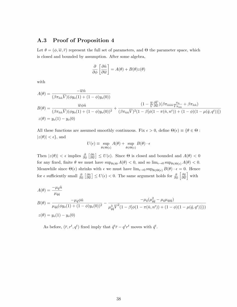
A.3 Proof of Proposition 4
Let θ = (φ,w, r) represent the full set of parameters, and Θ the parameter space, which
is closed and bounded by assumption. After some algebra,
∂
∂φ
[∂n̂
∂w
]= A(θ) +B(θ)z(θ)
with
A(θ) =−wn̂
(βπn̂n̂V )(φyo(1) + (1− φ)yo(0))
B(θ) =wφn̂
(βπn̂n̂V )(φyo(1) + (1− φ)yo(0))2+
(1− wV∂V∂w )(βπn̂n̂n̂
πn̂V πn̂n̂
+ βπn̂n̂)
(βπn̂n̂V )2(1− β[φ(1− π(n̂, nt)) + (1− φ)(1− µ(q̂, qt))])
z(θ) = yo(1)− yo(0)
All these functions are assumed smoothly continuous. Fix ε > 0, define Θ(ε) ≡ {θ ∈ Θ :
|z(θ)| < ε}, and
U(ε) ≡ supθ∈Θ(ε)
A(θ) + supθ∈Θ(ε)
B(θ) · ε
Then |z(θ)| < ε implies ∂∂φ
[∂n̂∂w
]≤ U(ε). Since Θ is closed and bounded and A(θ) < 0
for any fixed, finite θ we must have supθ∈ΘA(θ) < 0, and so limε→0 supθ∈Θ(ε)A(θ) < 0.
Meanwhile since Θ(ε) shrinks with ε we must have limε→0 supθ∈Θ(ε)B(θ) · ε = 0. Hence
for ε sufficiently small ∂∂φ
[∂n̂∂w
]≤ U(ε) < 0. The same argument holds for ∂
∂φ
[∂q̂∂w
]with
A(θ) =−µq̂n̂µq̂q̂
B(θ) =−µq̂φn̂
µq̂q̂(φyo(1) + (1− φ)yo(0))2−
−µq̂(µ2q̂q̂ − µq̂µq̂q̂q̂)
µ3q̂q̂V
2(1− β[φ(1− π(n̂, nt)) + (1− φ)(1− µ(q̂, qt))]))
z(θ) = yo(1)− yo(0)
As before, (r, rt, qt) fixed imply that q̂tr − qtrt moves with q̂t.
38
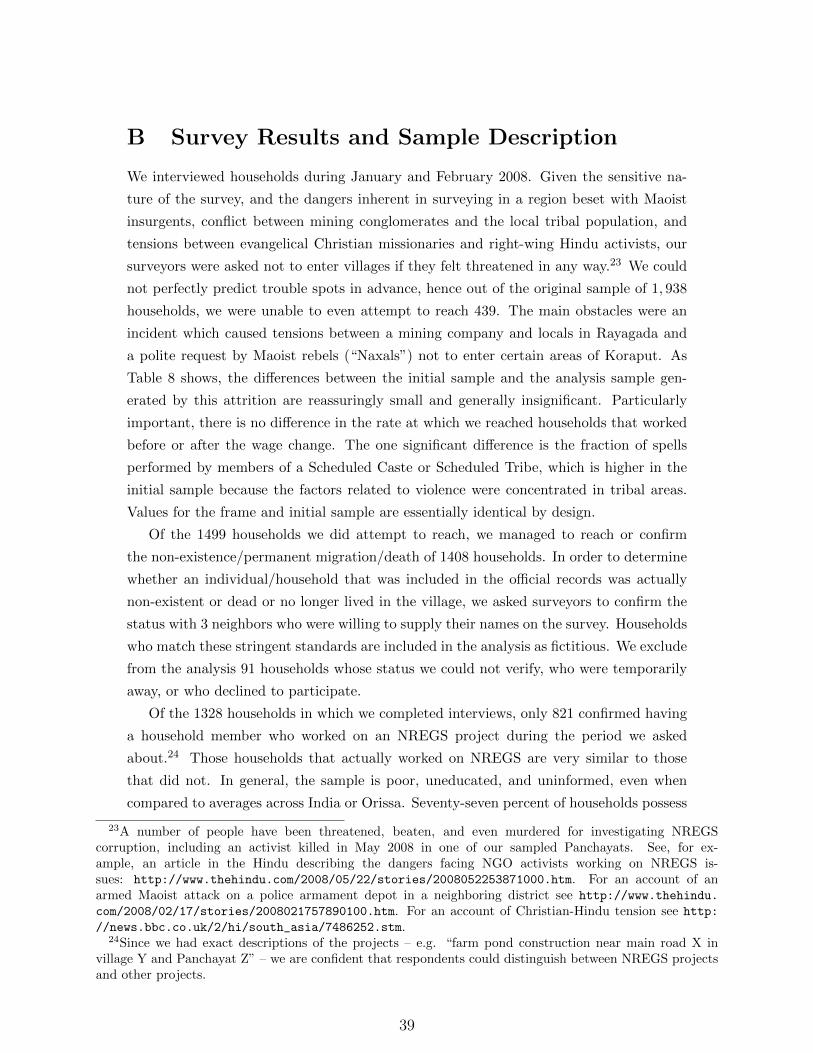
B Survey Results and Sample Description
We interviewed households during January and February 2008. Given the sensitive na-
ture of the survey, and the dangers inherent in surveying in a region beset with Maoist
insurgents, conflict between mining conglomerates and the local tribal population, and
tensions between evangelical Christian missionaries and right-wing Hindu activists, our
surveyors were asked not to enter villages if they felt threatened in any way.23 We could
not perfectly predict trouble spots in advance, hence out of the original sample of 1, 938
households, we were unable to even attempt to reach 439. The main obstacles were an
incident which caused tensions between a mining company and locals in Rayagada and
a polite request by Maoist rebels (“Naxals”) not to enter certain areas of Koraput. As
Table 8 shows, the differences between the initial sample and the analysis sample gen-
erated by this attrition are reassuringly small and generally insignificant. Particularly
important, there is no difference in the rate at which we reached households that worked
before or after the wage change. The one significant difference is the fraction of spells
performed by members of a Scheduled Caste or Scheduled Tribe, which is higher in the
initial sample because the factors related to violence were concentrated in tribal areas.
Values for the frame and initial sample are essentially identical by design.
Of the 1499 households we did attempt to reach, we managed to reach or confirm
the non-existence/permanent migration/death of 1408 households. In order to determine
whether an individual/household that was included in the official records was actually
non-existent or dead or no longer lived in the village, we asked surveyors to confirm the
status with 3 neighbors who were willing to supply their names on the survey. Households
who match these stringent standards are included in the analysis as fictitious. We exclude
from the analysis 91 households whose status we could not verify, who were temporarily
away, or who declined to participate.
Of the 1328 households in which we completed interviews, only 821 confirmed having
a household member who worked on an NREGS project during the period we asked
about.24 Those households that actually worked on NREGS are very similar to those
that did not. In general, the sample is poor, uneducated, and uninformed, even when
compared to averages across India or Orissa. Seventy-seven percent of households possess
23A number of people have been threatened, beaten, and even murdered for investigating NREGScorruption, including an activist killed in May 2008 in one of our sampled Panchayats. See, for ex-ample, an article in the Hindu describing the dangers facing NGO activists working on NREGS is-sues: http://www.thehindu.com/2008/05/22/stories/2008052253871000.htm. For an account of anarmed Maoist attack on a police armament depot in a neighboring district see http://www.thehindu.
com/2008/02/17/stories/2008021757890100.htm. For an account of Christian-Hindu tension see http:
//news.bbc.co.uk/2/hi/south_asia/7486252.stm.24Since we had exact descriptions of the projects – e.g. “farm pond construction near main road X in
village Y and Panchayat Z” – we are confident that respondents could distinguish between NREGS projectsand other projects.
39
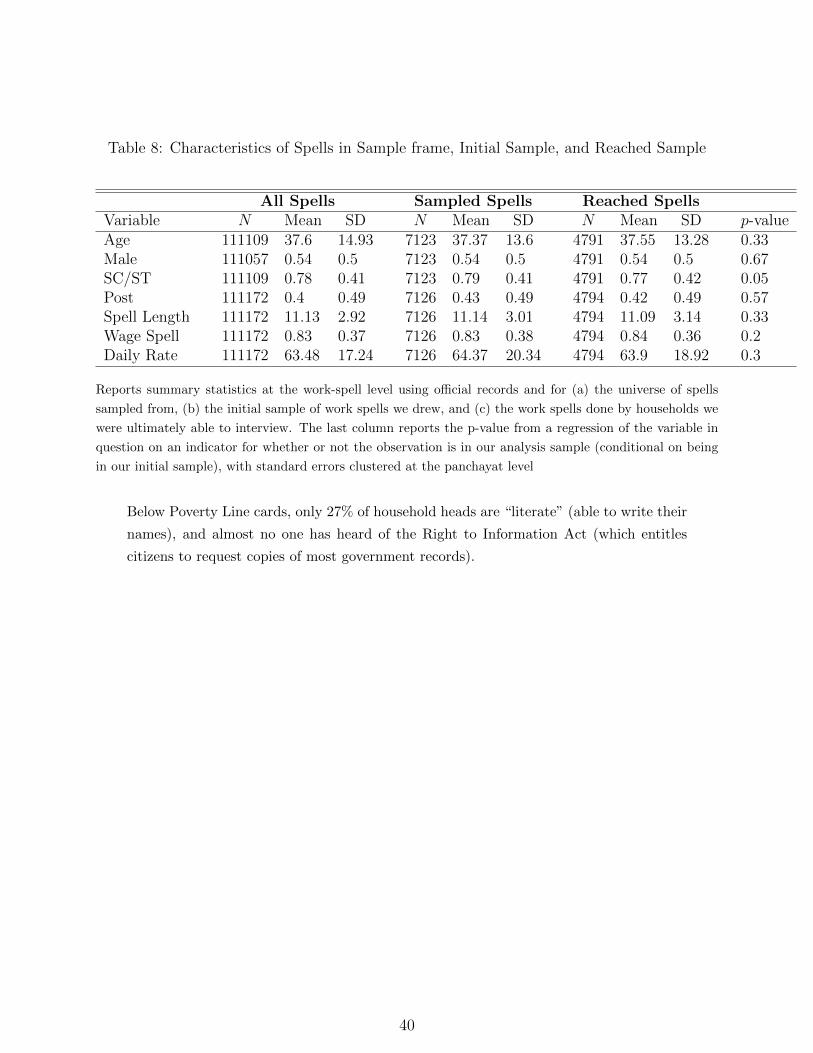
Table 8: Characteristics of Spells in Sample frame, Initial Sample, and Reached Sample
All Spells Sampled Spells Reached SpellsVariable N Mean SD N Mean SD N Mean SD p-valueAge 111109 37.6 14.93 7123 37.37 13.6 4791 37.55 13.28 0.33Male 111057 0.54 0.5 7123 0.54 0.5 4791 0.54 0.5 0.67SC/ST 111109 0.78 0.41 7123 0.79 0.41 4791 0.77 0.42 0.05Post 111172 0.4 0.49 7126 0.43 0.49 4794 0.42 0.49 0.57Spell Length 111172 11.13 2.92 7126 11.14 3.01 4794 11.09 3.14 0.33Wage Spell 111172 0.83 0.37 7126 0.83 0.38 4794 0.84 0.36 0.2Daily Rate 111172 63.48 17.24 7126 64.37 20.34 4794 63.9 18.92 0.3
Reports summary statistics at the work-spell level using official records and for (a) the universe of spells
sampled from, (b) the initial sample of work spells we drew, and (c) the work spells done by households we
were ultimately able to interview. The last column reports the p-value from a regression of the variable in
question on an indicator for whether or not the observation is in our analysis sample (conditional on being
in our initial sample), with standard errors clustered at the panchayat level
Below Poverty Line cards, only 27% of household heads are “literate” (able to write their
names), and almost no one has heard of the Right to Information Act (which entitles
citizens to request copies of most government records).
40