Corruption Dynamics: The Golden Goose Effect∗

Paul Niehaus†

UC San Diego, BREAD, and J-PAL

Sandip Sukhtankar‡

Dartmouth College, Harvard University, and J-PAL

August 31, 2012

Abstract

Theoretical work on disciplining corrupt agents has emphasized the role of expected futurerents – for example, efficiency wages. Yet taken seriously this approach implies that illicit futurerents should also deter corruption. We study this “golden goose” effect in the context of a statutorywage increase in India’s employment guarantee scheme, comparing official micro-records to originalhousehold survey data to measure corruption. We estimate large golden goose effects that reducedthe total impact of the wage increase on theft by roughly 64%. In short, rent expectations matter.

JEL codes: D73, H53, J30, K42, O12

Keywords: corruption, principal-agent problems, dynamics, workfare

∗We thank Nageeb Ali, Eric Edmonds, Edward Glaeser, Roger Gordon, Claudia Goldin, Gordon Hanson, LarryKatz, Asim Khwaja, Michael Kremer, Sendhil Mullainathan, Ben Olken, Rohini Pande, Andrei Shleifer, JonathanZinman, and seminar participants at Harvard, Yale, BREAD, Stanford, the World Bank, CGD, UNH, Indian Sta-tistical Institute-Delhi, NEUDC-Boston University, Dartmouth, and UCSD for helpful comments. Thanks also toManoj Ahuja, Arti Ahuja, and Kartikian Pandian for generous hospitality and insight into the way NREGS operatesin practice, and to Sanchit Kumar for adept research assistance. We acknowledge funding from the National ScienceFoundation (Grant SES-0752929), a Harvard Warburg Grant, a Harvard CID Grant, and a Harvard SAI Tata Sum-mer Travel Grant. Niehaus acknowledges support from a National Science Foundation Graduate Student ResearchFellowship; Sukhtankar acknowledges support from a Harvard University Multidisciplinary Program in Inequality &Social Policy Fellowship.†Department of Economics, University of California at San Diego, 9500 Gillman Drive #0508, San Diego, CA

92093-0508. pniehaus@ucsd.edu.‡Department of Economics, Dartmouth College, 326 Rockefeller Hall, Hanover, NH 03755.

sandip.sukhtankar@dartmouth.edu.

1

1 Introduction

Disciplining corrupt officials is a key governance challenge in developing countries.1 In an influential

early analysis Becker and Stigler (1974) argued that if there is some chance of detecting and

dismissing corrupt agents then the principal can mitigate the problem by paying an efficiency

wage. Intuitively, agents have an incentive to cheat less today in order to improve their chances of

earning a wage premium (or pension) tomorrow. Subsequent work has maintained this emphasis

on contracts designed to offer future rents.2

In contrast, the literature has put less emphasis on the role played by expectations of illicit

future rents. This paper focuses explicitly on the dynamic tradeoff between extracting rents today

and improving one’s chances of surviving to extract rents tomorrow. We call this latter motive

the “golden goose” effect to reflect the idea that agents want to preserve “the goose that lays the

golden eggs” (unlike the deplorably myopic farmer in the fable).3 We show that incorporating the

golden goose effect into standard models tends to weaken or even overturn the usual comparative

statics because of a generic tendency for static and dynamic effects to offset each other.4

To assess the relevance of this mechanism we gathered data from India’s largest rural welfare

program, the National Rural Employment Guarantee Scheme (NREGS). The scheme entitles every

rural household in India to up to 100 days of paid, on-demand employment per year; it is also

of intrinsic interest given that it covers roughly 11% of the world’s population. We obtained

disaggregated official records on participation, including the names and addresses of participating

households, the duration of each spell of employment and the amount of compensation paid. We

then independently surveyed a sample of these (alleged) beneficiaries to document the amounts of

work actually done and payments actually received. The gap between official and actual payments

– which includes both over-reporting of days and under-payment of wages – is the primary form

of corruption we study.5

Testing for golden goose effects requires an exogenous source of variation in anticipated rent-

extraction opportunities. We exploit a policy change: a 1 May 2007 increase in the statutory

wage due to program participants in the state of Orissa. A higher statutory wage means more

lucrative corruption opportunities for officials, since they receive more money for every fictitious

day of work reported. Importantly, the wage reform was enacted by policy-makers well removed

from the officials we study, making it plausibly exogenous. Because the wage increase was specific

to the state of Orissa we can also use data from the neighboring state of Andhra Pradesh as a

control in some specifications.

Interestingly, the effects of a wage change on daily wage over-reporting turn out to be theo-

retically ambiguous. There is an obvious static price effect: officials receive more money for every

1Recent work has shown how corruption constrains redistribution (Reinikka and Svensson 2004, Olken 2006),creates new market distortions (Sequeira and Djankov 2010) and hinders efforts to remedy existing ones (Bertrand,Djankov, Hanna and Mullainathan 2007).

2See Cadot (1987), Andvig and Moene (1990), Besley and McLaren (1993), Mookherjee and Png (1995), andAcemoglu and Verdier (2000), among others. Becker and Stigler’s (1974) model is a multi-period one but theyexamined a contract that entirely eliminates illicit rents. As we discuss below, the literature on electoral discipline isan important exception.

3Our usage differs from McMillan (2001), who uses “golden goose” to describe ex-ante investments by individualsthat a government may hold up ex-post. Commitment will not be an issue in our setting.

4Note that the framework here is one of observed types, as opposed to the career concerns framework in whichthe agent wishes to influence future perceptions of his ability (or honesty) (Holmstrom 1999).

5On the importance of measuring corruption directly, rather than using perceptions, see Olken (2009).

2

day of wage work they report, strengthening their incentives to over-report. If the wage increase

were temporary this would be the only effect. Following a permanent change, however, there is

also a dynamic golden goose effect: officials anticipate a more lucrative future, weakening their

incentives to over-report.

To separate out golden goose effects we exploit the fact that compensation on roughly 30%

of the NREGS projects in our sample was based on piece rates rather than a daily wage. This

heterogeneity reflects the fact that piece rates could not be implemented on some projects where

output was hard to measure. Because the schedule of projects had been fixed in advance of the

1 May 2007 wage change, and because piece rate schedules were not revised along with the daily

wage, the wage change should not have directly affected piece rate projects. Officials who were

managing piece rate projects at the time of the wage change often had wage projects planned in

the near future, however, and thus experienced a shift in their future rent expectations. This effect

should also have been stronger in proportion to the share of upcoming projects that were daily

wage. Theory thus predicts that the wage increase should (1) reduce theft from piece rate projects,

and (2) differentially reduce corruption in villages with more daily wage projects upcoming.

We take these predictions to panel data on corruption before and after the policy shock in 215

panchayats (villages). The data suggest that prices do matter: when statutory daily wages increase,

officials report more fictitious work on wage projects. Overall, the daily wage increase from Rs. 55

to Rs. 70 (combined with secular trends) increased the cost to the government per dollar received

by beneficiaries from $4.08 to $5.03. We also find evidence consistent with golden goose effects.

First, theft on piece rate projects in Orissa declined after the shock, both in absolute terms and

relative to neighboring Andhra Pradesh. Second, both daily-wage over-reporting and piece rate

theft fell differentially (the former significantly) in villages which subsequently executed a higher

share of daily wage projects. While some of the point estimates are imprecise, so that magnitudes

should be interpreted cautiously, they suggest large golden goose effects. Rough calculations imply

that theft increased by 64% less than it would have had the wage increase been temporary. This

point estimate need not be externally valid for other settings, of course; we merely emphasize that

dynamics appear to play a large role even in a setting where tenure is typically quite short.

To separate our interpretation from other substitution mechanisms we test for time-symmetry.

Intuitively, most substitution mechanisms imply that the effects of future rent expectations should

be similar to the effects of past and current rent realizations. For example, if the marginal value

of rents is decreasing so that officials become “satiated” then both past and future windfalls

should decrease current rent extraction. Empirically we find a consistent negative relationship

with future rent-extraction opportunities, but an inconsistent relationship with past rent-extraction

opportunities. We also analyze data on visits by superior officials to rule out confounding changes

in monitoring intensity.

Our analysis has four main implications for anti-corruption policy. First, it provides evidence

in support of the broad hypothesis that future rents matter, which is at the heart of the efficiency

wage concept. As Olken and Pande (2012) discuss, government wages have received a great deal

of attention, yet the empirical evidence has been limited to cross-country regressions and to the

indirect test in Di Tella and Schargrodsky (2003) who study the differential effects of an audit

crackdown. We simply exploit variation in expectations of illicit as opposed to licit rents to test

the same underlying mechanism.6

6As some NREGS officials are elected the results can also be read as supporting theories of electoral discipline in

3

Second, our data suggest that optimal contracts should take illicit as well as licit rents into

account. Comparing what we know about the compensation of officials we study to our estimates

of corruption implies that their illicit earnings are orders of magnitude greater than their licit wage

(150 to 1100 times wages), let alone their wage premium. Calculations that leave out these illicit

rents are unlikely to hit the mark.

Third, our data suggest that concerns about the “displacement” effects of anti-corruption work

should be taken seriously. As Yang (2008) discusses, the possibility that cracking down on one

kind of corruption may lead to increases in other kinds has been widely discussed but rarely tested.

Our data support this hypothesis. Indeed, the golden goose mechanism generates displacement

generically: any use of the “stick” that reduces future rent expectations also makes the “carrot” of

job security less motivating. The analysis thus complements Yang’s model based on non-convexities

in lawbreaking.

Finally, our results suggest that policy pilots should be interpreted carefully in weakly insti-

tutionalized settings. Simply put, a pilot generates different dynamic incentives than permanent

implementation. For example, distributing welfare benefits once does not generate future rent

expectations, while distributing them repeatedly does; a pilot may therefore appear to perform

artificially poorly. Auditing once does not reduce future rent expectations, while a regular program

of audits does; a pilot may therefore appear to perform artificially well. Generally speaking, ex-

pectations matter for interpreting results on monitoring (Di Tella and Schargrodsky 2003, Nagin,

Rebitzer, Sanders and Taylor 2002, Olken 2007) and on transparency more generally (Reinikka

and Svensson 2005, Ferraz and Finan 2008).

The rest of the paper is structured as follows: Section 2 describes the NREGS context, Section

3 lays out the theoretical framework, Section 4 describes data collection and estimation equations,

Section 5 presents results, and Section 6 concludes.

2 Contextual Background on the NREGS

India’s National Rural Employment Guarantee Scheme (now called the “Mahatma Gandhi Na-

tional Rural Employment Guarantee Act”) is a landmark effort to redistribute income to the rural

poor. The program was launched in February 2006 in the poorest 200 districts in India and as of

April 2008 covers the entire country (604 rural districts). The total proposed budget allocation for

the April 2010-March 2011 fiscal year is Rs. 401 billion (US$ 8.9 billion), which is 0.73% of 2008

GDP.7 It is likely that the steady-state cost will be higher as implementation is still incomplete in

many parts of the country. The following discussion describes the program as it was implemented

during our study period; some of the procedures described may have changed.

2.1 Statutory Operational Procedures

Each operational program cycle begins before the start of a fiscal year, when local governments at

the Gram Panchayat (GP or panchayat, lowest level of administration in the Indian government,

which voters must allow politicians some future rents in order to maintain control over them (Barro 1973, Ferejohn1986, Persson, Roland and Tabellini 1997, Ahlin 2005, Ferraz and Finan 2009).

7Costs: http://indiabudget.nic.in/ub2010-11/bh/bh1.pdf. GDP: http://mospi.nic.in/4_gdpind_cur.pdf.The central government must by law contribute at most 90% of total expenditure, the rest of the funding comingfrom the states.

4

comprising of a group of villages) and block (intermediate level of government between GPs and

districts) levels plan a “shelf” of projects to be undertaken during the upcoming year. The par-

ticular types of project allowed under the NREGS are typical of rural employment projects: road

construction and earthworks related to irrigation and water conservation predominate.

Projects also vary in the payment scheme they utilize: NREGS workers can be paid either on

a daily wage or a piece rate basis depending on the practicality of measuring output. There are

broad categories of projects that are paid on piece rate as opposed to daily wage; for example all

irrigation/water conservation projects which involve digging ditches are piece rate, while all road

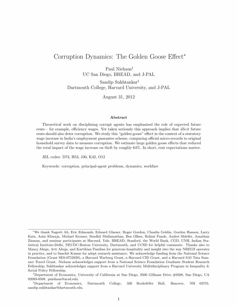
construction/paving projects are daily wage. Empirically it is the case that all the work done on

any particular project is generally compensated in the same manner (see Figure 1). Consequently

there are identifiable daily wage projects and piece rate projects. While according to statute the

project shelf should be proposed by village assemblies (Gram Sabhas), in practice higher up officials

at the Block and District level suggest and approve the shelf.

A key feature of the NREGS is that it is an unrestricted entitlement program: every household

in rural India has a right to 100 days of paid employment per year, with no eligibility requirements.8

To obtain work on a project, interested households must first apply for a jobcard.9 The jobcard

contains a list of household members, some basic demographic information, and blank spaces for

recording work and payment history. In principle, any household can obtain a jobcard for free at

either the panchayat or block administrative office. Jobcards in hand, workers can apply for work

at any time. The applicant must be assigned to a project within 15 days after submitting the

application; if not they are eligible for unemployment compensation. Applicants have no influence

over the choice of project.

At the work sites the panchayat officials record attendance (in the case of daily wage projects)

or measure output (in the piece rate case). They record this information both in workers’ jobcards

and in muster rolls which are sent to Block offices and digitized. The state and central governments

reimburse local governments on the basis of these electronic records. Most workers in our study

area received their wages in cash from the panchayat administration, although efforts to pay them

through banks are under way. As a transparency measure, all the official micro-data on payments

have been made publicly available through a web portal maintained by the central Ministry of

Rural Development (http://nrega.nic.in).

2.2 Implementing Officials

The officials in charge of implementing the program are mainly appointed bureaucrats at the block

(Block Development Officers, Junior Engineers, Assistant Engineers) and panchayat (Panchayat

Secretary, Field Assistants, Mates, etc) levels, with the exception of the elected chairman of the

Gram Panchayat (the “Sarpanch”). District level program officials, including the District Collector,

oversee block officials’ work. While in principal officials can be fired, suspended, or removed from

their jobs for misconduct, Article 311(2) of the Indian constitution says that no civil servant can be

dismissed without an official enquiry, which makes it difficult to fire someone outright in practice.

Suspensions and transfers into backwater jobs, however, are common punishments (Das 2001).

8Officials thus do not have an opportunity cost of allocating work to workers, as in Banerjee (1997).9Since each household is limited to 100 days of employment per year the definition of a household is important. In

NREGS guidelines a household is “a nuclear family comprising mother, father, and their children, and may includeany person wholly or substantially dependent on the head of the family” (Ministry of Rural Development 2006).

5

Because our analysis revolves around forward-looking optimization it is useful to understand

bureaucratic tenure in these jobs. Tenure for elected Sarpanchs is five years. Tenure for appointed

bureaucrats is typically shorter, primarily because transfers are used as a disciplinary tool and as

a way for political parties to bestow favors. Iyer and Mani (2009) document that the district-level

Indian Administrative Service (IAS) officers who oversee local officials stay in a job for a year

and a half on average, and since they often move with their staff this implies that the tenure of

lower-level officials is at least as short. In Gujarat, Block Development Officers keep that post for

an average of sixteen months (Zwart (1994), p 94). Given the small but significant pay differential

between private sector and public sector jobs at this level (Das 2001) and the short tenure, local

public officials often seek opportunities for extracting rents.

2.3 Rent Extraction, Monitoring and Enforcement

Officials’ opportunities for illicit gain include control over project selection; bribes for obtaining

jobcards and/or employment; and embezzlement from the materials and labor budgets. We focus

on theft from the labor budget, which we can cleanly measure. The labor budget is required by

law to exceed 60% of total spending, and in fact we find that theft in this category is so extensive

that even if all of the 40% allocated to materials were stolen, the labor budget would still be the

larger source of illegal rents.10

Theft from the labor budget comes in two conceptually distinct forms. First, officials can

under-pay workers for the work they have done (theft from beneficiaries). Second, officials can

over-report the amount of work done when they send their reports up the hierarchy (theft from

taxpayers). For example, a worker who worked for 10 days on a daily wage project when the

statutory minimum wage was Rs. 55 per day might receive only Rs. 45 per day in take-home pay.

The official might report that the worker had worked for 20 days rather than 10. His total rents

would then equal 55 · 20− 45 · 10 = 650 rupees, the sum of the two sorts of theft.

A key difference between theft from beneficiaries and theft from taxpayers lies in the way they

are monitored. Underpaid workers who know they are underpaid could either complain to someone

at the block or district headquarters or simply leave for the private sector. On the other hand,

workers have less incentive to monitor over-reporting: because the program’s budget is not fixed,

a rupee stolen through over-reporting does not mean a rupee less for the workers. In principal the

NREGS Operational Guidelines address this issue by calling both for bottom-up monitoring via

Gram Sabhas (village meetings), local Vigilance and Monitoring Committees, and bi-annual “social

audits,” and also top-down monitoring via inspection of works by superior officials (100% of works

checked by block officials, 10% by district officials, and 2% by state officials). The guidelines do

not provide incentives for auditing or link audit results to budget allocations, however. In practice

there was no systematic audit process in Orissa during the period we study (in contrast with, for

example, the setting in Olken (2007)). What top-down monitoring did exist consisted primarily

of informal tracking and worksite visits by officials. For example, some block and district officials

we interviewed use the NREGS’s management information system to track aggregate quantities of

work done on various projects and compare these to technical estimates or their own best guesses

of the resources required.

Officials caught cheating face a positive but small probability of getting punished. Program

10We also found that bribes paid to obtain jobcards are uncommon (17% report paying positive amounts) andsmall (averaging Rs. 10 conditional on being positive).

6

guidelines call for “speedy action against [corrupt] officials” but do not lay out specific penalties. In

practice the most likely penalty is suspension or transferal to a less desirable job; for elected officials

it is loss of office. The Chief Minister at one point claimed to have initiated action against nearly

half the Block Development Officers in the state, but some of this is likely political posturing.11

A more reliable source may be the records of OREGS-Watch, a loose online coalition of non-

governmental organizations that monitor NREGS in Orissa; their reports note numerous instances

of officials being caught and suspended (http://groups.google.co.in/group/oregs-watch).

The common pattern in these cases was incontrovertible proof brought to the office of the District

Collector, followed immediately by the suspension of the guilty official and in some cases by the

recovery of the stolen funds. In one case in Boudh district, for example, the offending official was

caught within two weeks of the misdemeanor, the money recovered and the official suspended.12

2.4 Wage-Setting

Our estimation strategy exploits an increase in statutory program wages in the eastern state of

Orissa in 2007. Such wage hikes were common due to the incentives generated by the NREGS’s

funding pattern. The central (federal) government pays 100% of the unskilled labor budget, and

75% of the materials budget (defined to include the cost of skilled labor) (Ministry of Law and

Justice 2005). The states, however, set wages and piece-rates. This provision creates strong

incentives for state politicians to raise wage rates, benefiting their constituents at the central

government’s expense.

We study the effects of a change in the statutory daily wage for unskilled workers in Orissa

from Rs. 55 to Rs. 70. This change was announced on April 28th, 2007 and went into effect

on May 1st, 2007. Importantly, this policy change did not directly affect payments on piece rate

projects, and it was specific to Orissa (did not affect neighboring Andhra Pradesh).13 Note that

wages for three categories of higher-skilled labor were also raised on 1 May from Rs. 65/75/85 to

Rs. 80/90/100. Because skilled wages are rarely reported in our data (6.5% of work spells) and

their use varies primarily within-project (65% of the variation) we focus our theoretical discussion

around a single wage rate.

3 Dynamic Rent Extraction

Following Becker and Stigler (1974) a large theoretical literature has studied the use of dismissal

threats to motivate corruptible agents. Dismissal typically matters in these models because agents

who are not dismissed expect to receive compensation greater than their outside option – a wage

premium or a pension, for example. In a dynamic setting, however, an agent’s expected future rents

include both an exogenous licit component provided by the contract and also an endogenous illicit

11http://www.orissadiary.com/Shownews.asp?id=620112http://www.dailypioneer.com/59458/Action-taken-after-study-finds-fake-muster-roll-in-Boudh.

html.13The NREGS implementation guidelines state that the states should “devise productivity norms for all the tasks

listed under piece-rate works for the different local conditions of soil, slope and geology types in such a way thatnormal work for the prescribed duration of work results in earnings at least equal to the wage rate.” In practice,however, this occurs haphazardly and with long and variable lags. In Orissa wages were revised on 1 May 2007 butthe piece rate schedule was not amended until 16 August 2007, a month and a half after our study period ends, andat that time some rates were lowered rather than raised.

7

component determined by their own future corrupt behavior. For example, an official thinking

about whether to take a bribe today will rationally take into account the bribe revenue he expects

to earn tomorrow. In this section we develop a dynamic model to examine the role that such

expectations play in decision-making. We specialize the framework to our context by modeling

the kinds of corruption that we see in our data but also comment on broader implications.

Time is discrete. An infinitely-lived official and a group of N infinitely-lived workers seek to

maximize their discounted earnings stream:

ui(t) =

∞∑τ=t

βτ−tyi(τ) (3.1)

where yi(τ) are the earnings of agent i in period τ . Additional players with identical preferences

wait in the wings to replace the official should he be fired.

In each period exactly one NREGS project is active. We abstract from simultaneous ongoing

projects primarily to simplify the exposition; it is also true, however, that most of the panchayats

in our sample have either one or zero projects active at all times during our study period. Let

ωt = 1 indicate that the active project at time t is a wage project, and ωt = 0 that it is a piece

rate project. We represent the “shelf” of projects as an infinite stochastic stream of projects: at

the beginning of each period a random project is drawn from the shelf with

φ ≡ P(ωt = 1|ωt−1, ωt−2, . . .) (3.2)

We suppose that all agents know φ but do not know exactly which projects will be implemented

in the future. At the cost of a small loss of realism, this approach ensures that the dynamic

environment is stationary and greatly simplifies the expression of comparative statics. It also

permits a close analogy between the model and our empirical work, in which the fraction of future

projects that are daily wage (a measure of φ) plays a key role. We treat φ as exogenous here

since de jure it should be predetermined, but will also test below whether it responds to the wage

change.

Each worker inelastically supplies one indivisible unit of labor in each period. We interpret a

unit flexibly as either a day (in the case of daily wage projects) or as a unit of output (in the case

of piece-rate projects). Labor may be expended on an NREGS project or in the private sector,

where worker i can earn wt (rt). Let nt (qt) be the number of days (output units) supplied to

the project when ωt = 1 (ωt = 0), and let and wti (rti) be the wage (piece-rate) that participating

worker i receives. This need not equal the statutory wage w (the statutory piece rate r).

NREGS wages and employment levels emerge from bargaining between the official and the

workers. In principal workers have two sources of bargaining power: they can threaten to complain

if the official pays them less than the statutory rate w (r), or can simply leave for the private

sector and earn wt (rt. Which of these threat points matters in practice is of course an empirical

question. In a companion paper we study this issue in some detail; we find that the wages workers’

receive bear little relationship to the statutory wage but closely track variation in local market

wages (Niehaus and Sukhtankar 2012). Motivated by these data, we model equilibrium wages and

participation choices as tracking market wages (wti = wt and nt = nt(wt)). We further simplify

matters by abstracting from time variation in the market wage, so wt = w and nt = n.

Participation n and the average participant’s wage w (piece rate r) are thus predetermined

8

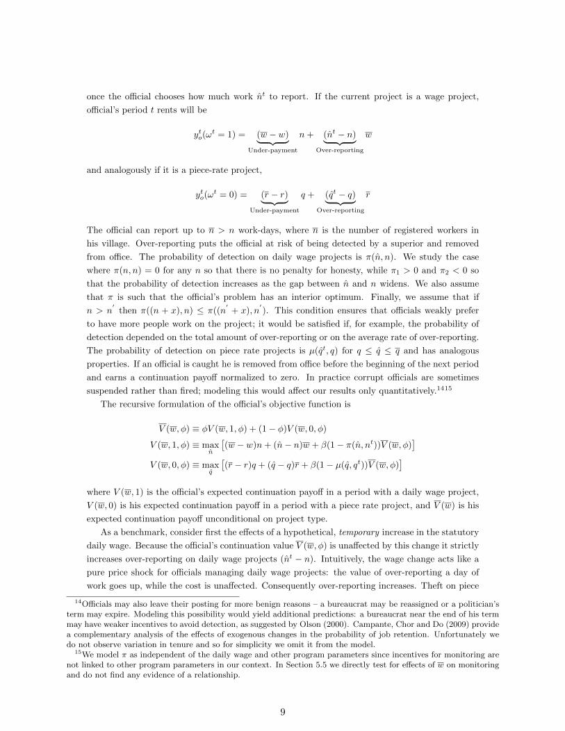
once the official chooses how much work nt to report. If the current project is a wage project,

official’s period t rents will be

yto(ωt = 1) = (w − w)︸ ︷︷ ︸

Under-payment

n+ (nt − n)︸ ︷︷ ︸Over-reporting

w

and analogously if it is a piece-rate project,

yto(ωt = 0) = (r − r)︸ ︷︷ ︸

Under-payment

q + (qt − q)︸ ︷︷ ︸Over-reporting

r

The official can report up to n > n work-days, where n is the number of registered workers in

his village. Over-reporting puts the official at risk of being detected by a superior and removed

from office. The probability of detection on daily wage projects is π(n, n). We study the case

where π(n, n) = 0 for any n so that there is no penalty for honesty, while π1 > 0 and π2 < 0 so

that the probability of detection increases as the gap between n and n widens. We also assume

that π is such that the official’s problem has an interior optimum. Finally, we assume that if

n > n′

then π((n + x), n) ≤ π((n′

+ x), n′). This condition ensures that officials weakly prefer

to have more people work on the project; it would be satisfied if, for example, the probability of

detection depended on the total amount of over-reporting or on the average rate of over-reporting.

The probability of detection on piece rate projects is µ(qt, q) for q ≤ q ≤ q and has analogous

properties. If an official is caught he is removed from office before the beginning of the next period

and earns a continuation payoff normalized to zero. In practice corrupt officials are sometimes

suspended rather than fired; modeling this would affect our results only quantitatively.1415

The recursive formulation of the official’s objective function is

V (w, φ) ≡ φV (w, 1, φ) + (1− φ)V (w, 0, φ)

V (w, 1, φ) ≡ maxn

[(w − w)n+ (n− n)w + β(1− π(n, nt))V (w, φ)

]V (w, 0, φ) ≡ max

q

[(r − r)q + (q − q)r + β(1− µ(q, qt))V (w, φ)

]where V (w, 1) is the official’s expected continuation payoff in a period with a daily wage project,

V (w, 0) is his expected continuation payoff in a period with a piece rate project, and V (w) is his

expected continuation payoff unconditional on project type.

As a benchmark, consider first the effects of a hypothetical, temporary increase in the statutory

daily wage. Because the official’s continuation value V (w, φ) is unaffected by this change it strictly

increases over-reporting on daily wage projects (nt − n). Intuitively, the wage change acts like a

pure price shock for officials managing daily wage projects: the value of over-reporting a day of

work goes up, while the cost is unaffected. Consequently over-reporting increases. Theft on piece

14Officials may also leave their posting for more benign reasons – a bureaucrat may be reassigned or a politician’sterm may expire. Modeling this possibility would yield additional predictions: a bureaucrat near the end of his termmay have weaker incentives to avoid detection, as suggested by Olson (2000). Campante, Chor and Do (2009) providea complementary analysis of the effects of exogenous changes in the probability of job retention. Unfortunately wedo not observe variation in tenure and so for simplicity we omit it from the model.

15We model π as independent of the daily wage and other program parameters since incentives for monitoring arenot linked to other program parameters in our context. In Section 5.5 we directly test for effects of w on monitoringand do not find any evidence of a relationship.

9

rate projects (qtr−qr) does not change, on the other hand, since neither the costs nor the benefits

of stealing change.

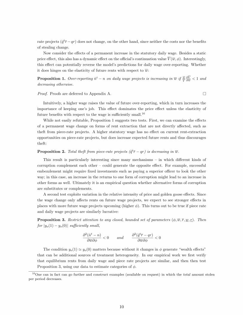
Now consider the effects of a permanent increase in the statutory daily wage. Besides a static

price effect, this also has a dynamic effect on the official’s continuation value V (w, φ). Interestingly,

this effect can potentially reverse the model’s predictions for daily wage over-reporting. Whether

it does hinges on the elasticity of future rents with respect to w:

Proposition 1. Over-reporting nt − n on daily wage projects is increasing in w if wV∂V∂w < 1 and

decreasing otherwise.

Proof. Proofs are deferred to Appendix A.

Intuitively, a higher wage raises the value of future over-reporting, which in turn increases the

importance of keeping one’s job. This effect dominates the price effect unless the elasticity of

future benefits with respect to the wage is sufficiently small.16

While not easily refutable, Proposition 1 suggests two tests. First, we can examine the effects

of a permanent wage change on forms of rent extraction that are not directly affected, such as

theft from piece-rate projects. A higher statutory wage has no effect on current rent-extraction

opportunities on piece-rate projects, but does increase expected future rents and thus discourages

theft:

Proposition 2. Total theft from piece-rate projects (qtr − qr) is decreasing in w.

This result is particularly interesting since many mechanisms – in which different kinds of

corruption complement each other – could generate the opposite effect. For example, successful

embezzlement might require fixed investments such as paying a superior officer to look the other

way; in this case, an increase in the returns to one form of corruption might lead to an increase in

other forms as well. Ultimately it is an empirical question whether alternative forms of corruption

are substitutes or complements.

A second test exploits variation in the relative intensity of price and golden goose effects. Since

the wage change only affects rents on future wage projects, we expect to see stronger effects in

places with more future wage projects upcoming (higher φ). This turns out to be true if piece rate

and daily wage projects are similarly lucrative:

Proposition 3. Restrict attention to any closed, bounded set of parameters (φ,w, r, w, r). Then

for |yo(1)− yo(0)| sufficiently small,

∂2(nt − n)

∂w∂φ< 0 and

∂2(qtr − qr)∂w∂φ

< 0

The condition yo(1) ' yo(0) matters because without it changes in φ generate “wealth effects”

that can be additional sources of treatment heterogeneity. In our empirical work we first verify

that equilibrium rents from daily wage and piece rate projects are similar, and then then test

Proposition 3, using our data to estimate categories of φ.

16One can in fact can go further and construct examples (available on request) in which the total amount stolenper period decreases.

10

3.1 Effects of Wages and Monitoring

The results above characterize the effects of a wage reform to guide our empirical work. Earlier

work, on the other hand, has emphasized the probability of audit and the official’s wage as key

exogenous parameters. To relate our model to this literature we next characterize their effects.

To formalize the probability of an audit let π(n, n) = γπ(n, n), where γ is the probability a

daily-wage project is audited and π the conditional probability of conviction. Then one can show

that a one-period increase in γ decreases over-reporting on daily wage projects and has no effect on

theft from piece rate projects. A permanent increase in γ, on the other hand, generates a smaller

decrease – or even an increase – in daily-wage over-reporting, and increases theft from piece rate

projects. The contrast between these results yields a simple lesson for empirical work: the right

interpretation of empirical evidence on the effects of a crackdown depends on whether officials

perceived it to be temporary or permanent. In particular, temporary crackdowns generate larger

reductions in corruption than permanent ones, and should thus be interpreted cautiously as guides

to policy-making.

Efficiency wages, on the other hand, work here just as they would in a one-shot game. To see

this let V (w, φ) = φV (w, 1, φ) + (1 − φ)V (w, 0, φ) + W where W ≥ 0 is a wage premium paid to

the official in each period until he is not dismissed. It is straightforward to show that all forms

of corruption are decreasing in W . Intuitively, the efficiency wage has no price effects and only

deterrent effects. As this example illustrates the theory’s novel predictions hinge not on dynamics

per se but on the dynamic implications of future corrupt rents.

3.2 Alternative Substitution Mechanisms

Some of our framework’s implications could also be generated by alternative substitution mech-

anisms. We conclude our theoretical discussion with a brief overview of these mechanisms and

highlight a key distinction between them and the golden goose effect: the latter predicts that only

future rent expectations, and not past rent realizations, affect current behavior. We will exploit

this asymmetry below to examine which story best fits our data.

One possible substitution mechanism involves the “production function” for corruption. Anec-

dotal evidence suggests that the bulk of corruption in our setting simply involves writing one

number on paper instead of another. Suppose, however, that this requires the use of some scarce

input that can be shifted across time (e.g. effort). Then the wage shock would induce officials

to optimally re-allocate this input across time, giving rise to patterns similar to those we predict.

Second, if officials care about things other than consumption then the wage shock might have

income effects. The expectation of large future rents would lower the expected relative marginal

utility of income now, leading to lower corruption. In an extreme case of income effects officials

might even “target” a particular income level. Finally, empirical tests could potentially be sensitive

to issues of time aggregation. In our empirical work we treat the day as the basic unit of time,

but monitoring might be based on less frequent observations. This would mechanically imply that

officials expecting to steal more tomorrow would steal less today, since the probability of detection

would depend on the sum of today’s report and tomorrow’s.

One difference between the golden goose effect and these mechanisms is that the former is

purely forward-looking while the latter are time-symmetric, in that they predict that increases

in both past and future corruption opportunities should reduce corruption today. Consider the

11

“input” model: suppose that the official can extract rents Rt today and Rt+1 tomorrow only if

f(Rt, Rt+1) ≤ 0 for some increasing function f . Clearly any factor that increases Rt+1 must

therefore decrease Rt, generating what might look like a golden goose effect. Similarly, however,

any factor that increases Rt must decrease Rt+1, so that shocks to lagged rent extraction also

negatively effect rent extraction today. An analogous argument applies to the monitoring story

(for example, let the probability of an investigation be f(Rt + Rt+1)). Finally, consider a simple

model with income effects in which officials maximize U(Rt +Rt+1)−D(Rt, Rt+1) where U is an

increasing, concave function and D is the expected non-monetary disutility of punishments. (The

income-targeting story is a limit case of this example.) Provided D12 is not too negative, changes

in D that lower the cost of Rt+1 will induce substitution away from Rt due to diminishing marginal

utility (U ′′ < 0). This also implies the converse, however.

4 Empirical Approach

4.1 Official Data

To test the theoretical predictions in Section 3 we adopt an audit approach, comparing official

micro-data on wage payments and program participation to original household survey data col-

lected from the same (alleged) beneficiaries. The official data we use are publicly available on a

central website (http://nrega.nic.in). Data available at the level of the individual worker in-

clude names, ages, addresses, caste status, and unique household jobcard number. Data available

at the level of the work spell include number of days worked, name and identification number of

the project worked on, and amount paid. Descriptive information on the nature of the projects and

the names of the officials responsible for implementation are also available. It is straight-forward

to infer whether a project paid daily wages or piece rates because there are only a few allowed

daily wage rates.17 (Figure 1)

We used as our sample frame the official records for the states of Orissa and Andhra Pradesh as

downloaded in January 2008, six months after our study period, to allow time for all the relevant

data to be uploaded. As a cross-check we also downloaded the official records a second time

in March 2008. We found that the records for Orissa remained essentially unchanged, but that

the number of work spells recorded for Andhra Pradesh increased by roughly 10%. These new

observations were spread uniformly across space and time and so do not appear to have resulted

from delays in processing records for specific panchayats or projects. They do, however, generate

some uncertainty about the representativeness of our AP sample frame. We will emphasize the

Orissa data and use AP as a control only in Table 6.

We sampled from the list of officially recorded NREGS work spells during the period March

1st, 2007 to June 30th, 2007 in Gajapati, Koraput, and Rayagada districts in Orissa. Within these

districts, we restricted our attention to blocks at the border with AP. We sampled 60% of the

Gram Panchayats within study blocks, stratified by whether the position of GP chief executive

had been reserved for women. (Chattopadhyay and Duflo (2004) find evidence suggesting that

reservations affect levels of corruption.) Within these panchayats we sampled 2.8 percent of work

spells, stratified by Panchayat, by whether the project was implemented by the block or the

panchayat administration, by whether the project was a daily wage or piece-rate project, and by

17We designate a project as daily wage if more than 95% of the wages paid are these amounts.

12

whether the work spell was before or after the daily wage shock. This yielded a total of 1938

households. We set out to interview all adult members of these households about their NREGS

participation, so that our measures of corruption would not be affected if work done by one member

was mistakenly reported as having been done by another. Details on survey results and a sample

description are in Appendix B.

4.2 Survey Coverage

We asked respondents retroactively about spells of work they did between March 1, 2007 and June

30, 2007. A spell of work is a well-defined concept within the NREGS: it is an uninterrupted period

of up to two weeks employment on a single project. For each spell we asked subjects the dates

during which they worked, the number of days worked, what project they worked on, whether they

were paid on a piece rate or daily wage basis, what payment they received, and in the case of piece

rate projects what quantity of work they did. In addition to the survey of program participants,

we also administered a separate questionnaire to village elders with questions on labor market

conditions, agricultural seasons and official visits in the village.

While imperfect recall could potentially be a concern given the lag between the study period

and our survey, we designed the survey instrument and trained enumerators to jog respondents’

memories: for example, using major holidays as reference points. The results were encouraging:

we obtained information on at least the month in which work was done for 93% of the spells

in our sample. We do not find significant differential recall problems over time: in a variety of

specifications including location fixed effects and individual controls such as age and education,

subjects’ estimated probability of recalling exact dates increases by only 0.7%–2.2% per month

and is not statistically significant. Since our main tests exploit discrete time-series changes while

controlling for smooth trends, these patterns should not introduce bias. Subjects’ recall was

facilitated by the fact that the NREGS was a new and salient program, and spells of work were

likely to be memorable and distinct compared to other employment. Subjects are also more likely

to keep track of their participation and compensation given that they do not necessarily get paid

what they are owed or on time. The one place where recall does matter is that recipients do have

difficulty recalling the quantity of work done on piece rate projects – the amount of earth they

moved, volume of rocks they split, etc. Consequently in our empirical work we treat theft on piece

rate projects as unitary (qtr − qtrt in terms of the model).

Survey interviews were framed to minimize other potential threats to the accuracy and veracity

of respondents self-reports. We made clear that we were conducting academic research and did not

work for the government, to discourage them from claiming fictitious underpayment; in the end

most respondents reported that they had been paid what they thought they were owed. None of

the interviewed households have income close to the taxable level and will have ever paid income

taxes, so there are no tax motives for underreporting. Conversely, officials had little need to secure

workers’ collusion in their over-reporting. A worker could only supply a signature, which has little

relevance when most people cannot write their own name. There is also no reason to believe

that respondents would under-report corruption for fear of reprisals, since they could not have

known how many days they were reported as having worked in the official data. Finally and most

importantly, there is no reason to think any of these issues would lead to differential biases (which

would affect our results) and not just level ones (which would not). Niehaus and Sukhtankar (2012)

confirms that the wage shock had no effect on the self-reported variables we use in our analysis.

13

4.3 Empirical Specifications

Our empirical analysis includes all spells of work from our survey data that contain information

on at least the month of the spell, the number of days worked, and the wages received. We impute

start or end dates if unavailable, and construct time-series of survey reports of work done and

wages paid by aggregating data at the panchayat-day level for the sample period. We distribute

days worked equally over the month if neither start nor end date are available, and equally in the

period between the start date and end date if the number of days worked is less than the period

between the start and end dates. Table C.1 gives a numerical example of the construction of our

dependent variables. Similarly, we construct time-series of the official data by aggregating official

reports of work done and wage paid of only those households who we interviewed or confirmed

as fictitious over the sample period. Table 2 presents summary statistics of the main outcome

variables; the discrepancy between official and survey amounts is stark, but at leakage rates of

around 75% within the range of corruption estimates across developing nations, other programs in

India, as well as other estimates of corruption in NREGS in Orissa.18

Our first empirical strategy is to regress officially reported outcomes ypt for panchayat p and

day t on actual outcomes ypt as reported by participants, an indicator Shockt for the post 1

May period, and a number of time-varying controls summarized by Tt including a polynomial in

day-of-year to capture long-term trends, a polynomial in day-of-month to capture periodicity, and

an indicator for major holidays. Certain specifications also include regression-discontinuity type

controls where the Shock indicator is interacted with time trends. Finally, we include indicators for

political reservations Rp and in some specifications district fixed effects δd(p) to capture variation

in program implementation across locations:19

ypt = β0 + β1ypt + β2Shockt + T′

t γ +R′pζ + δd(p) + εpt (4.1)

Standard errors are clustered at the panchayat as well as the day level using multi-way clustering.

Note that if ypt were correlated one-for-one with ypt then this approach would be equivalent to

using ypt − ypt as the dependent variable, while if not our approach is less restrictive. We have

also implemented the more restrictive approach, however, and the results are if anything stronger

(see Table 7 and the discussion in Section 5.4).

Identification in (4.1) rests on the assumption that unobserved factors affecting ypt are orthog-

onal to Shockt after controlling for the other regressors. To relax this assumption we also exploit

data from the neighboring district of Vizianagaram in Andhra Pradesh to control for unobserved

time-varying effects common to the geographic region under study. There are, however, several

caveats. First, we can only implement this strategy when studying piece-rate theft, since essentially

all projects in Andhra Pradesh are piece-rate. Second, as noted above a substantial number of new

observations appeared in the official Vizianagaram records after we selected our sample. Finally,

Andhra Pradesh made two revisions to its schedule of piece rates during our sample period, the

latter of which took effect on March 25th, 2007. Because of its proximity to the daily wage change

18For example, Reinikka and Svensson (2004) find rates of 87% in a schooling program in Uganda, while Ferraz,Finan and Moreira (2012) find leakage of up to 55% in a schooling program in Brazil. In the Indian context, Khera(2011) finds leakage rates of almost 90% in the flagship food subsidy program (TPDS) in Bihar, while a study doneby an NGO (Center for Science and Environment) on corruption in the NREGS in Orissa found almost precisely thesame numbers (75%).

19Key political positions in some villages are reserved by law for women and/or ethnic minorities.

14

in Orissa this shock limits the value of Andhra Pradesh as a control for high-frequency confounds,

although it is still useful for low-frequency ones. Keeping these limitations in mind, we estimate

ypt = β0 + β1ypt + β2ORshockt ∗ORp + β3APShock1t ∗APp + β4APShock2t ∗APp+ β5ORshockt + β6APShock1t + β7APShock2t +ORp

+ T′

t γ +R′pζ + δd(p) + εpt (4.2)

where ORp (APp) indicates panchayats in Orissa (Andhra Pradesh). The coefficient of interest in

this specification is β2, the differential change in corruption in the post-shock period in Orissa.

To test for the differential effects of the wage change predicted by Proposition 3 we need an

empirical analogue to φ, the probability that a future project in our model is a daily wage project.

Given that many of the panchayats in our data only implement wage projects, we partition the

set of panchayats into those that do and do not ever run piece-rate projects and estimate:

ypt = β0 + β1ypt + β2Shockt + β3Shockt ∗AlwaysDWpt + β4AlwaysDWpt

+ T′

t γ +R′pζ + δd(p) + εpt (4.3)

for daily-wage outcomes. Our model predicts β2 > 0 while β3 < 0. We can also apply a similar

idea to piece-rate outcomes, replacing AlwaysDW with AlwaysPR. In this case we expect β2 < 0

while β3 > 0.

While specification (4.3) has a simple differences-in-differences interpretation, we can obtain a

more stringest test of the theory by isolating the differential response attributable only to future

daily-wage projects. To do this we must define, for every panchayat and every day, the proportion

of upcoming work that is daily-wage. We accomplish this by (1) defining a “project-day” as a

day on which a particular project is running, where a project is running if work on that project

as been reported in the past and will be reported in the future, and then (2) calculating for

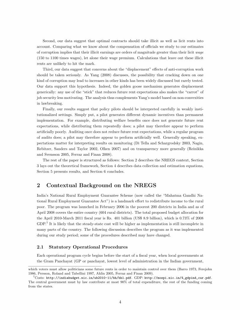
each panchayat-day observation the fraction FwdWageFrac of project-days in the upcoming two

months that are daily wage project-days. Figure 4 plots the distribution of FwdWageFrac in our

sample. Given the existence of clear mass points at 0 and 1 we adopt a flexible approach, binning

the data into three categories: one where FwdWageFrac = 0 (the omitted category), one where

0 < FwdWageFrac < 1 (FdwSome), and one where FwdWageFrac = 1 (FdwAll).20 We then

allow the effects of the wage change to vary across these categories:

ypt = β0 + β1ypt + β2Shockt + β3Shockt ∗ FdwAllpt + β4FdwAllpt

+ β5Shockt ∗ FdwSomept + β6FdwSomept + T′

t γ +R′pζ + δd(p) + εpt (4.4)

Note that a key goal in constructing these forward-looking measures is to capture variation in the

proportion of daily wage projects on the panchayat’s “shelf” of projects without also including

endogenous variation in the amount of work reported. This is the reason that we focus on whether

projects are ongoing, rather than the number of person-days of work purportedly done. We show

below that the FwdWageFrac variable is indeed uncorrelated with the wage shock. It is also

important to note that if it were endogenously related to the wage change we would expect the

20We have also estimated more restrictive models in which FwdWageFrac enters linearly and obtained qualitativelysimilar results (available on request).

15

resulting bias to work against us rather than for us: panchayats that increased their corruption

most in response to the shock would be the most likely to switch to wage projects, generating a

positive bias on the interaction term.

To provide more insight into whether past opportunities for corruption matter in the same way

as future opportunities, we construct bins based on an analogous measure BkWageFrac of the

fraction of project-days in the preceeding two months that were daily wage and estimate:21

ypt = β0 + β1ypt + β2Shockt + β3Shockt ∗ FdwAllpt + β4Shockt ∗BdwAllpt+ β5Shockt ∗ FdwSomept + β6Shockt ∗BdwSomept

+ β7FdwAllpt + β8BdwAllpt + β9FdwSomept + β10BdwSomept

+ T′

t γ +R′pζ + δd(p) + εpt (4.5)

Our model predicts β3 < 0 with no prediction about β4, while if time-symmetric mechanisms are

important then we should see β3 ' β4 < 0.

Table 2 presents summary statistics of the main variables used in our regressions.

5 Results: The Golden Goose Effect

5.1 Preliminaries: Wages, Projects and Rents

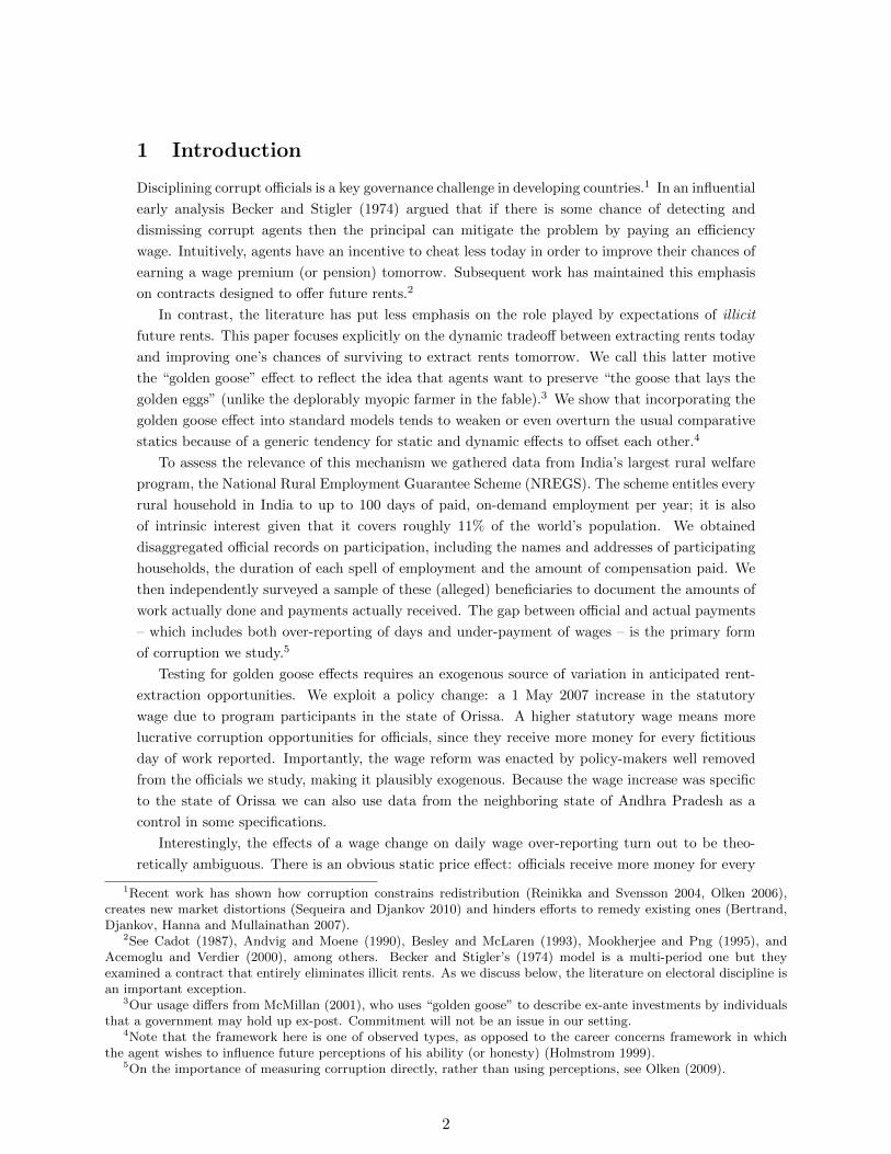
We begin with tests of the main identifying assumptions. Figure 2 shows that the policy change was

actually implemented: the average wage rate officially claimed on daily wage projects however near

Rs. 55 until May 1st and then jumps up sharply thereafter. Interestingly, it does not immediately

or permanently reach the new statutory wage of Rs. 70. This is because not all panchayats

implemented the change – some continued to claim the old rates after May 1st, likely because they

were not immediately informed about the change.22 23 We also examined changes in the use of

the “skilled” wage categories after 1 May and found a small decrease in the proportion of wage

spells for which skilled wages were claimed, from 7.5% prior to 1 May to 6.3% after 1 May. While

we cannot reliably assess the “true” skill level of any given spell, this decrease is consistent with

the hypothesis that there is some skill inflation going on and that golden goose effects led officials

to do less of it after the wage change.

Figure 2 also reveals that the wage rate actually received by workers was unaffected by the

shock; if anything it trends slightly downwards, though this effect is largely compositional and

disappears once we control for district effects. In a companion paper we examine the determination

of actual wages in some detail (Niehaus and Sukhtankar 2012). We find, inter alia, that while 72%

of respondents were aware that the wage had changed and 81% of these correctly identified the

new wage, these “aware” workers did not earn higher wages after 1 May relative to their less-aware

peers. Similarly, literate workers were no more likely to see their wages increase. For further

21The correlation between FwdWageFrac and BkWageFrac is 0.75 within district, 0.6 within blocks, and 0.11within panchayats; between FwdWageFrac and the current daily wage fractions the correlations are 0.85, 0.76, and0.41 respectively. The results must be interpreted with these correlations in mind.

22In Niehaus and Sukhtankar (2012) we show that panchayats that are closer to block and district offices are morelikely to implement the wage change.

23This interpretation suggests an additional test: all our predictions should hold only in panchayats that actuallyimplemented the wage change. We pursued this strategy, but unfortunately there are insufficiently many non-implementing panchayats for us to precisely estimate the difference.

16

analysis an interpretation of these facts we refer the reader to the companion paper; our analysis

here will focus on testing our theoretical predictions about over-reporting, taking the observed

wage dynamics as given.2425

Second, we check whether pre-shock rent extraction from daily wage and piece rate projects are

similar, as predicated by Proposition 3. Dividing total theft in the two categories of projects by

the number of actual days worked on those projects, we find that the rate of theft per day worked

is very similar pre-shock; Rs. 236 per actual day worked in daily wage projects as opposed to Rs.

221 in piece rate projects.26 This is important both because it allows us to test Proposition 3 and

also because it implies that officials would have had little incentive to distort project types prior

to the wage change.

Finally, we check whether project shelf composition responds endogenously to the wage shock.

In principal it is fixed at the start of the fiscal year (March 2007), but if officials had scope to

reclassify or re-order projects they might have prioritized wage projects. In fact the fraction of

projects that are daily wage fell from 74% before 1 May to 72% afterwards. More formally, Table 3

reports regressions of FwdWageFrac on an indicator for the shock along with time controls. The

point estimates are insignificant and correspond to a 0.02 standard deviation change in project

composition. These results corroborate the testimony of block-level officials that the shelf of

projects and payment schemes is pre-determined. They are also natural given that changing the

designation of project is a relatively observable form of cheating.

In unreported results we also examined whether project shelf composition is correlated with

key political variables like reservations for women and minorities at the sarpanch and samiti rep-

resentative level; with the number of locally active NGOs; with village elders’ perceptions of the

relative wealth and relative political activism of the village; and with indicators for visits from

block and district officials. In general we found no significant correlations; the one exception we

uncovered was the corelation with the share of the population belonging to scheduled castes, and

since very few scheduled castes live in our study area this explains very little variation in the shelf.

We have also included these characteristics directly as controls in our regressions and they do not

change our findings (available on request).

5.2 Over-reporting of Days Worked in Daily Wage Projects

We begin our core analysis by examining the reported number of days worked on daily wage

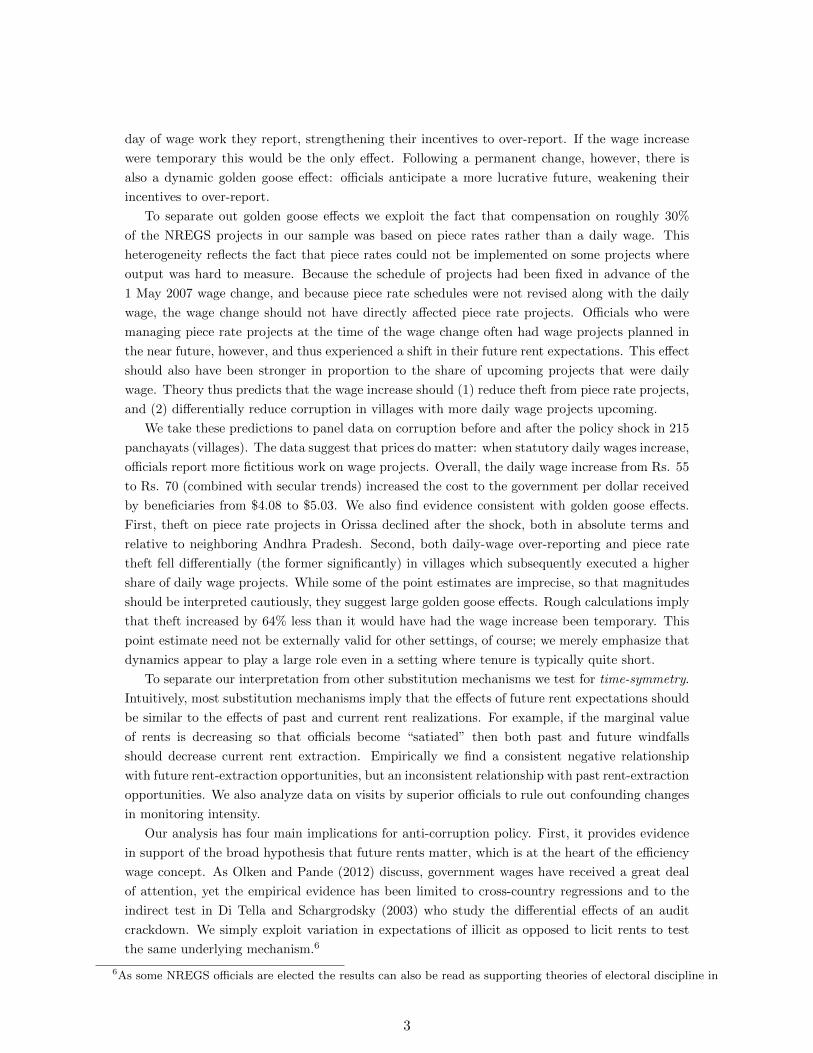
projects. Panels (a) and (b) of Figure 3 show the evolution of over-reporting over time – i.e. the

difference between the number of days of work reported by officials and by households. Note that

the sharp downward spikes generally occur on major holidays, suggesting that officials perceive

24Another intriguing feature of Figure 2 is that during the first month of our study period workers were on averageover -paid. This pattern is driven by observations from Gajapati district where prevailing market wages were higherthan the statutory program wage. If officials do not pay this prevailing market wage, workers will not participate inthe program. If workers do not participate, officials cannot extract rents. Hence, according to local NGOs, officials insuch areas overpay workers for participation, even though they report the correct statutory program wage on officialreports, making up the difference by over-reporting days worked.

25Cross-sectional variation in wages suggests another potential test of the golden goose effect: we would expect tosee officials taking more risk in locations where the market wage w is larger relative to the statutory wage w. Inresults available on request we find that rent extraction is indeed (insignificantly) higher in panchayats with lowermarket wages, as predicted by their endowments of land and labor.

26These figures are scaled to reflect misreporting of days worked as daily wage projects when in fact they weredesignated as piece rate projects in the official data. In general, this kind of misreporting is rare: 82% of spells arereported correctly, whereas 15% of piece rate spells are reported as daily wage spells.

17

over-reporting on holidays as particularly risky. The superimposed fitted models summarize an

exploratory regression-discontinuity analysis: we fit polynomials in day-of-year to the aggregate

time series and allowed the coefficients to vary before and after the wage change took effect on

1 May. The fitted models suggest that there was a slight increase in daily-wage over-reporting

following the shock. This may seem surprising given the obvious effect of the wage hike on incentives

for over-reporting, but as Proposition 1 suggests there may also be a countervailing dynamic effect.

Columns I-III in Panel A of Table 4 present a disaggregated analysis based on Equation 4.1.

Column I presents estimates of the basic specification (Equation 4.1) with a linear time trend

and no location effects; Column II adds district fixed effects, while Column III adds a linear trend

interacted with the shock term. Consistently across these specifications we find that official reports

are significantly higher when more actual work was done and, conditional on actual work done,

significantly lower on major holidays (not reported). The estimated impact of the wage shock,

on the other hand, is positive but not significant in each specification. To examine whether this

is due to an offsetting dynamic effect, Columns IV-VI of Panel A separate panchayats that ran

solely daily-wage projects from those that also ran piece rate projects (Equation 4.3). We find a

differential reduction in over-reporting in the daily-wage only panchayats, significant at the 10%

level; summing the point estimates implies a small reduction in over-reporting in these locations.

In contrast, the estimated effect of the wage change in panchayats that ran at least some piece

rate projects is larger and significant in Column IV. This suggests the presence of a substitution

effect that is muting the overall impact of the wage change.

To further isolate the portion of this differential effect that is attributable to having future

daily-wage projects, and in order to test Proposition 3, Columns I-III of Panel B report estimates

of the interaction between the wage shock and categories of our constructed FwdWageFrac mea-

sure (Equation 4.4). The estimated direct effect of the wage hike increases again and is significant

at the 5% level; the interpretation is that this is the price effect that would obtain in a panchayat

with no future daily wage projects planned. Note that this result also rules out alternative ex-

planation based on strong diminishing marginal returns to income, such as income “targeting”.

The differential effect in panchayats with solely wage projects upcoming is negative and significant

at the 10% level, while the differential effect in panchayats with a mix of upcoming projects is

negative but insignificant, providing support for Proposition 3.27

To better understand what drives these patterns of substitution, Columns IV-VI of Panel B

present specifications that allow for both the future and the past to predict responsiveness to

the shock (Equation 4.5). The direct effect of the shock remains positive and is significant. The

differential change in corruption in panchayats with only daily-wage projects upcoming is negative,

larger, and highly significant, confirming a strong substitution pattern. The analogous differential

change for panchayats that had only run daily-wage projects in the past is positive and insignificant,

which is inconsistent with time-symmetric interpretations of our forward-looking estimates. We

do estimate a significant negative differential effect in panchayats that had implemented a mix of

projects in the past, however. In contrast to the forward-looking results, this result is not robust to

replacing categories of the FwdWageFrac variable with the variable itself in our empirical model

27One potential concern about these results is that intertemporal substitution occurs mechanically because of the100 day limit on participation per household-year. In practice, however, we found that this limit was rarely reached.During fiscal year 2006-2007 only 4% of jobcards in our study area in Orissa reached 100 days, and all panchayatsin our sample had a significant number of jobcards with less than 100 days – 95% of the cards on average and at aminimum 22%.

18

(not reported). This, and the fact that we do not find differential drops in panchayats with only

wage projects in the past, lead us to treat it with some caution.

5.3 Theft in Piece Rate Projects

We turn next to theft from piece-rate projects. This margin of corruption provides an attractive

test for golden goose effects because it was not directly affected by the wage change, so that only

dynamic effects should apply (Proposition 2). Panels (c) and (d) of Figure 3 show the evolution of

the gap between official and actual payments on piece-rate projects over the sample period, again

with fitted regression-discontinuity specifications superimposed. Theft was unusually low in May

following the wage shock; indeed, officially reported payments fell while actual payments rose. The

fitted models reflect this, consistently estimating a significant discrete drop on 1 May. Note also

that theft rebounded in June; while various factors could be at play, this is also broadly consistent

with a dynamic model since NREGS projects largely cease operation during the monsoons starting

in late June in Orissa. This implies that future rent expectations were falling steadily through

May and June.

Turning to a disaggregated analysis, Table 5 mirrors Table 4 but with the total reported

payments on piece rate projects as the dependent variable and total actual payments on piece-rate

projects as a predictor. In Column I of Panel A the main effect of the wage shock is negative

and significant at the 5% level, providing strong support for Proposition 2. The magnitude of

the coefficient – about Rs. 78 per day – is also economically meaningful compared to the average

theft per panchayat-day observation prior to the shock of Rs. 102. Columns II-III show that

while the coefficient does not change much, standard errors are slightly larger and the result is

hence significant at the 10% level. Columns IV-VI again separate those panchayats that ran only

piece rate projects from those that ran both types of projects; as expected the coefficient on the

interaction terms is positive, though insignificant. The estimated change in panchayats with both

kinds of projects is larger and more precisely estimated. Note that the sum of the coefficient on

the shock and the interaction term is not statistically significantly different from zero, suggesting

that the shock itself had no effect on panchayats that only ran piece rate projects.

As before, Panel B adds interactions between the shock and the forward and backward fraction

of daily wage projects. As with daily wage over-reporting we find a negative differential effect of the

shock in panchayats with all projects in the future being daily wage, and a positive coefficient on

the interaction between the shock and past high daily wage fractions. None of these estimates are

statistically significant, however. In general our power to estimate piece rate effects is limited by

the relative scarcity of piece-rate projects in Orissa. (For example, even the indicator for holidays,

which is consistently statistically significant in daily wage models, is imprecisely estimated in

piece-rate models.) Overall the estimated differential effects provide only suggestive evidence.

To obtain a more powerful test for Proposition 2 and address concerns about time-varying

confounds we next use Andhra Pradesh as a control. Table 6 reports estimates of Equation 4.2,

the differences-in-differences specification. The Orissa-specific effect of the daily wage shock in

Orissa is negative, larger than the first-differences estimate, and significant across all specifications.

Subject to the caveats described above, these estimates support the golden goose hypothesis.

19

5.4 Robustness Checks

For our preferred estimators we use the fraction of daily wage project-days in the upcoming two

months as the key interaction variable. A two-month window is sensible on several grounds. First,

longer forecasts of project shelf composition would not likely be relevant given that (a) the tenure

of bureaucrats in the relevant postings is quite short (approximately a year), and (b) very little

NREGS activity takes place once the monsoon season starts in earnest. Second, as per program

guidelines official reports are aggregated bi-weekly, so that it is plausible for an official to be

detected and punished within a two-month window. Nevertheless, columns I and II (VI and VII)

of Table 7 examine the sensitivity of the daily wage (piece rate) results to using one-month and

three-month windows. Results using a one-month window are similar and if anything stronger

than our baseline estimates. Results using a three-month window are somewhat smaller and not

statistically significant but are qualitatively similar, as one would expect if the three-month window

absorbs large periods of very little NREGS activity during the monsoon season.

Another alternative interpretation is that the wage shock did have differential effects but that

these were driven by other variables correlated with project shelf composition. The leading concern

in this context would be a relationship with the reservation of key political posts for women or

disadvantaged minorities. We checked earlier that shelf composition was not significantly correlated

with reservations, and these are also included as controls in all our specifications. We can further

include interactions between reservation categories and the wage change directly as controls in

our regressions. Columns III and VIII include indicators for each type of reservation (women,

Scheduled Castes, and Scheduled Tribes) and their interactions with the wage shock. This makes

the daily wage results stronger: both the positive main effect and the negative differential effect

are significant at the 5% level. The piece rate results, on the other hand, are largely unchanged.28

A third issue has to do with the exact timing of the effects we are attributing to the May 1st

policy change. Equation 4.4 implicitly assumes that the dynamic effects of the wage change take

effect at the same point in time as the static ones. If, however, officials learned about the wage

change before it took place then dynamic effects might begin earlier than the direct, static ones.

The 1 May wage change we study was the culmination of a process that began on 10 January with

the publication of a proposal to change wages, and it is possible that officials acquired information

over time about whether or not the proposal would be implemented. To explore whether our

causal interpretation of the coefficients on the post-May indicator is correct we re-ran our main

specifications using more flexible functions of time. Columns IV and IX of Table 7 report results

using indicators for each month (we ran similar specifications using bi-weekly dummies and reached

similar conclusions). In general the estimates are imprecise. There is some evidence – significant

for piece rate theft – that the differential effect of FwdWageFrac (though not the direct effect

of the shock) begins earlier in April. This is consistent with the view that at least some officials

learned about the wage change before it took place and began adjusting accordingly.

We have also examined the sensitivity of the results to allowing for quadratic trend controls; an

analogous set of tables in Appendix C reports these estimates (results for even higher-order trend

controls available on request). Higher-order polynomials have little effect on any of our results.

Finally, we examine the effects of using the difference ypt − ypt between official and actual

quantities as the dependent variable. Recall that this is equivalent to our approach if the true

28The estimated main effect switches from an insignificant negative effect to an insignificant positive one. Note,however, that this is the estimate for panchayats without any reservations, which make up only 3% of our sample.

20

relationship between those quantities is linear with slope 1, but otherwise is more restrictive. In

practice, imposing that restriction makes little difference for the results (Columns V and X). We

have also used the difference in total amounts extracted as the dependent variables, and as Table

8 shows again the results are very similar. This table also shows various other outcome variables:

the total rents combined from piece rate and daily wage projects, as well as official reports for

only “fictitious” households. The daily wage results for the fictitious households are strongly

statistically significant.

5.5 Is Monitoring Affected?

Another potential concern is that the intensity with which officials were monitored by their su-

pervisors changed around the same time as the daily wage change. If panchayats with more

wage projects upcoming experienced the largest increases in scrutiny this could explain the role

of FwdWageFrac in predicting responses to the wage shock. Of course, if this were true then

again one would expect BkWageFrac to play a similar role. Moreover, there is no a priori rea-

son to expect monitoring intensity to change: official notifications and instructions regarding the

wage change did not include any provisions regarding monitoring, and officials and the block and

panchayat level do not have implicit incentives to monitor linked to the amount of corruption (for

example, it is not the case that a detecting official earns a reward proportional to the amount the

detected official stole). Nevertheless, one would like direct evidence on this point.

To test for changes in monitoring we use data from our village-level survey on the most recent

visit to each village by the Block Development Officer (BDO) and the District Collector, the two

officials responsible for monitoring NREGS implementation at the panchayat level. Of course these

visits could have been for planning as well as monitoring purposes. In our Orissa sample, 62%

of panchayats had a BDO visit and 24% had a Collector visit since the beginning of the NREGS

in 2005. For these panchayats, we can test whether the likelihood of a visit went up after May

of 2007. Let t be the month in which a given panchayat was last visited by an official.29 We

suppose that the probability of the panchayat receiving a visit is independent (but not identical)

across months, as would be the case under optimal monitoring with symmetric information. Call

p(τ |θ, d) be the probability that a panchayat in district d receives a visit at time τ . Assume that

p has the logit form

p(t|θ, d) =exp{δd + γ1(t ≥ t∗) + f(t)}

1 + exp{δd + γ1(t ≥ t∗) + f(t)}(5.1)

If we had data on all official visits then we could estimate p(·|θ, d) directly. Because we only

observe the date of the most recent visit, we focus instead on the probability that the panchayat’s

last visit was at time t:

f(t|θ, d) = p(t|θ, d) ·ΠTτ=t+1(1− p(τ |θ, d)) (5.2)

Similarly, the probability that a panchayat did not receive a visit since the beginning of the NREGS

is

ΠTτ=t(1− p(τ |θ, d)) (5.3)

29In a small number of panchayats respondents could only remember the year, and not the month, of the most recentvisit by an official. We allow these observations to contribute to the likelihood function by simply calculating theprobability that the most recent visit fell in the given year. Our results are insensitive to omitting these observations.

21

where t is the NREGS start date. We estimate this model via maximum likelihood for both BDOs

and Collectors and for various specifications of p, in each case testing the null γ = 0. Table 9 reports

the results. The estimate of γ is positive but small and insignificant for BDOs; for collectors it

is positive and insignificant when controlling linearly for time and is significantly negative when

controlling for a quadratic in time. In short, we find no evidence of an increase in monitoring

intensity associated with the change in the daily wage.30

5.6 Interpreting Magnitudes

Given the confidence intervals around some of our coefficients, their magnitudes should be inter-

preted cautiously. With that caveat in mind we provide two calculations as benchmarks. First, we

compare the actual increase in theft due to the shock to the counterfactual effect of a temporary

wage hike without golden goose effects. We estimate that the permanent increase in daily wages

that we study raised theft by 64% less than a temporary increase of the same magnitude would

have, indicating that golden goose effects had a substantial “dampening” effect.31 However, the

90% confidence interval around that estimate is 8-120%, suggesting that this number must be

interpreted with caution. Second, we compare the magnitude of golden goose effects to the effects

of other anti-corruption interventions studied in the literature. We estimate that the dynamic

effects of the wage change lowered daily wage over-reporting and piece rate theft by 49% and

77%, respectively.32 These are meaningful effect sizes in comparison with other estimates from

the literature. For example, Olken (2007) estimates that increasing the probability of audit from

4% to 100% reduced corruption on Indonesian road projects by 30%; Ferraz and Finan (2009)

estimate that Brazilian mayors who are eligible for re-election misappropriate 27% fewer resources

than those who are not.

For policy purposes it would be informative to conduct a complete calibration of our model.

Unfortunately this is infeasible without richer data on all the sources of rent which a corrupt

official would lose if suspended or fired, and the value of their outside options. We can, however,

provide some sense of whether NREGS rents are a significant source of income relative to licit

compensation. We estimate total NREGS rents per panchayat (or block) per month by calculating

30One natural question is how closely officials’ expectations of changes in monitoring intensity corresponded toactual changes. While we cannot directly measure their beliefs, we can examine changes in monitoring surroundingearlier wages changes, which arguably shed light on what officials might reasonable have expected following the 1 May2007 reform. We estimated models analogous to those in Table 9 for two earlier reforms, a February 2006 daily wageincrease and an April 2006 piece rate increase. We find that the estimated impact of these reforms (not reported) onvisit probabilities is negative in all but one specification. We read these results as suggestive that officials should ifanything have expected a small reduction in monitoring.

31We estimate the actual increase in theft due to the shock as the sum of three components: (a) a mechanicalcomponent equal to the predicted quantity of daily wage over-reporting absent the shock multiplied by the changein the average daily wage, (b) a behavioral response in daily-wage over-reporting, which we estimate using thecoefficients from Column II, Panel B of Table 4, and (c) a negative behavioral response in piece-rate theft, estimatedusing the coefficient in Column II, Panel A of Table 5 (a conservative assumption given that the difference-in-differenceestimates of the latter effect are larger). We sum these effects to obtain an estimate ∆actual of the total effect ofthe shock on rent extraction. To construct a counterfactual estimate of the effect ∆counter of a temporary wage hikewe perform a similar calculation but omit the contributions of the piece rate regressions and the forward-lookinginteraction term in the daily wage regressions. Putting these pieces together, we estimate ∆counter−∆actual

∆counter= 64%.

32We estimate golden goose effects on daily wage over-reporting as the interaction coefficient from Column II, PanelB of Table 4 multiplied by the average fraction of future projects that are daily wage, divided by mean daily wageover-reporting prior to the shock. Similarly we estimate golden goose effects on piece rate theft as the coefficient inColumn II, Panel A of Table 5 divided by mean piece rate theft prior to the shock.

22

the difference between actual and reported payments in our sample multiplied by the inverse of

the sampling probability, and compare these to sarpanch honorariums and BDO salaries as per

the Government of Orissa’s payscales (based on 6th Central Pay Commission). The contrasts

are stark. The estimated rate of rent extraction per panchayat is roughly 150 times the rate at

which sarpanchs are compensated, and the rate per block is 1,100 times the rate at which Block

Development Officers are compensated. These figures clearly suggest that optimal contracts should

take the influence of illicit rents into account.

6 Conclusion

Dismissal, suspension, and transfer are standard tools for disciplining corrupt agents. We show

that these incentives generate a “golden goose” effect: as steady-state opportunities to extract rent

increase the value of continuing in office increases and this induces agents to act more cautiously.

This dynamic mechanism tends to dampen, and may reverse, the predictions of static models.

We test for golden goose effects using panel data on corruption in India’s National Rural

Employment Guarantee Scheme, exploiting an exogenous increase in program wages to construct

tests. We find two forms of evidence consistent with our theory: higher daily wages lead to lower

theft from piece rate projects, and differentially lower theft in areas with a higher proportion of

daily wage projects upcoming. Rough calculations based on the point estimates imply that these

effects reduced the increase in corruption generated by the wage change by approximately 64%.

Future work might focus on the longer-term implications of this effect for rent extraction.

23

References

Acemoglu, Daron and Thierry Verdier, “The Choice between Market Failures and Corrup-tion,” American Economic Review, March 2000, 90 (1), 194–211.

Ahlin, Christian, “Effects and (In)tractability of Decentralized Corruption,” mimeo, VanderbiltUniversity December 2005.

Andvig, Jens Chr. and Karl Ove Moene, “How corruption may corrupt,” Journal of Eco-nomic Behavior & Organization, January 1990, 13 (1), 63–76.

Banerjee, Abhijit V, “A Theory of Misgovernance,” The Quarterly Journal of Economics,November 1997, 112 (4), 1289–1332.

Barro, Robert, “The Control of Politicians, an Economic Model,” Public Choice, March 1973,14 (1), 19–42.

Becker, Gary S. and George J. Stigler, “Law Enforcement, Malfeasance, and Compensationof Enforcers,” The Journal of Legal Studies, 1974, 3 (1), 1–18.

Bertrand, Marianne, Simeon Djankov, Rema Hanna, and Sendhil Mullainathan, “Ob-taining a Driver’s License in India: An Experimental Approach to Studying Corruption,” TheQuarterly Journal of Economics, November 2007, 122 (4), 1639–1676.

Besley, Timothy and John McLaren, “Taxes and Bribery: The Role of Wage Incentives,”Economic Journal, January 1993, 103 (416), 119–41.

Cadot, Olivier, “Corruption as a gamble,” Journal of Public Economics, July 1987, 33 (2),223–244.

Campante, Felipe, Davin Chor, and Quoc-Anh Do, “Instability and the Incentives forCorruption,” Economics & Politics, March 2009, 21 (1), 42–92.

Chattopadhyay, Raghabendra and Esther Duflo, “Women as Policy Makers: Evidence froma Randomized Policy Experiment in India,” Econometrica, 09 2004, 72 (5), 1409–1443.

Das, S.K., Public Office, Private Interest: Bureaucracy and Corruption in India, New Delhi:Oxford University Press, 2001.

de Zwart, Frank, The Bureaucratic Merry-Go-Round, Amsterdam: Amsterdam University Press,1994.

Ferejohn, John, “Incumbent performance and electoral control,” Public Choice, January 1986,50 (1-3), 5–25.

Ferraz, Claudio and Frederico Finan, “Exposing Corrupt Politicians: The Effects of Brazil’sPublicly Released Audits on Electoral Outcomes,” The Quarterly Journal of Economics, 052008, 123 (2), 703–745.

and , “Electoral Accountability and Corruption: Evidence from the Audits of LocalGovernments,” NBER Working Papers 14937, National Bureau of Economic Research, IncApril 2009.

, , and Daniela Moreira, “Corrupting Learning: Evidence from Missing Federal Edu-cation Funds in Brazil,” Working Paper 18150, National Bureau of Economic Research June2012.

Holmstrom, Bengt, “Managerial Incentive Problems: A Dynamic Perspective,” Review of Eco-nomic Studies, January 1999, 66 (1), 169–82.

Iyer, Lakshmi and Anandi Mani, “Traveling Agents: Political Change and BureaucraticTurnover in India,” Working Paper 09-006, Harvard Business School 2009.

Khera, Reetika, “Trends in Diversion of PDS Grain,” Technical Report 198, Centre for Devel-opment Economics, Delhi School of Economics March 2011.

McMillan, Margaret, “Why Kill The Golden Goose? A Political-Economy Model Of ExportTaxation,” The Review of Economics and Statistics, February 2001, 83 (1), 170–184.

24

Ministry of Law and Justice, “The National Rural Employment Guarantee Act, 2005,” TheGazette of India, September 2005.

Ministry of Rural Development, The National Rural Employment Guarantee Act 2005: Op-eration Guidelines 2006, 2nd ed. 2006.

Mookherjee, Dilip and I P L Png, “Corruptible Law Enforcers: How Should They Be Com-pensated?,” Economic Journal, January 1995, 105 (428), 145–59.

Nagin, Daniel S., James B. Rebitzer, Seth Sanders, and Lowell J. Taylor, “Monitor-ing, Motivation, and Management: The Determinants of Opportunistic Behavior in a FieldExperiment,” American Economic Review, September 2002, 92 (4), 850–873.

Niehaus, Paul and Sandip Sukhtankar, “The Marginal Rate of Corruption in Public Pro-grams,” Technical Report, Dartmouth College 2012.

Olken, Benjamin A., “Corruption and the costs of redistribution: Micro evidence from Indone-sia,” Journal of Public Economics, May 2006, 90 (4-5), 853–870.

, “Monitoring Corruption: Evidence from a Field Experiment in Indonesia,” Journal of Po-litical Economy, April 2007, 115 (2), 200–249.

, “Corruption perceptions vs. corruption reality,” Journal of Public Economics, August 2009,93 (7-8), 950–964.

and Rohini Pande, “Corruption in Developing Countries,” Annual Review of Economics,2012, 4 (1).

Olson, Mancur, Power and Prosperity: Outgrowing Communist and Capitalist Dictatorships,New York: Basic Books, 2000.

Persson, Torsten, Gerard Roland, and Guido Tabellini, “Separation of Powers and PoliticalAccountability,” The Quarterly Journal of Economics, November 1997, 112 (4), 1163–1202.

Reinikka, Ritva and Jakob Svensson, “Local Capture: Evidence From a Central GovernmentTransfer Program in Uganda,” The Quarterly Journal of Economics, May 2004, 119 (2),678–704.

and , “Fighting Corruption to Improve Schooling: Evidence from a Newspaper Cam-paign in Uganda,” Journal of the European Economic Association, 04/05 2005, 3 (2-3), 259–267.

Sequeira, Sandra and Simeon Djankov, “An Empirical Study of Corruption in Ports,” Tech-nical Report, London School of Economics September 2010.

Tella, Rafael Di and Ernesto Schargrodsky, “The Role of Wages and Auditing during aCrackdown on Corruption in the City of Buenos Aires,” Journal of Law & Economics, April2003, 46 (1), 269–92.

Yang, Dean, “Can Enforcement Backfire? Crime Displacement in the Context of Customs Reformin the Philippines,” The Review of Economics and Statistics, November 2008, 90 (1), 1–14.

25

A Proofs

A.1 Proof of Proposition 1

The official’s problem during daily wage periods is

maxn

[(w − wt)nt + (n− nt)w + β(1− π(n, nt))V (w, φ)

]The posited attributes of π ensure that this problem has an interior solution satisfying w =

βπn(n, nt)V (w, φ). Differentiating with respect to w yields

∂n

∂w=

1− βπn ∂V∂wβπnnV (w, φ)

Substitution in the first-order condition yields

∂n

∂w=

1− wV∂V∂w

βπnnV (w, φ)

from which (and πnn > 0) the result is apparent.

A.2 Proof of Proposition 2

The official’s problem during piece rate periods is

maxq

[(r − rt)qt + (q − qt)r + β(1− µ(q, qt))V (w, φ)

]The posited attributes of µ ensure that this problem has an interior solution satisfying the Kuhn-

Tucker condition r = βµq(q, qt)V (w, φ). Since (r, rt, qt) are fixed we know that qtr − qtrt moves

with qt. Differentiating with respect to w yields

∂q

∂w=−βµq ∂V∂w

βµqqV (w, φ)

Since µqq > 0 it is sufficient to show ∂V∂w > 0. By the envelope theorem

∂V

∂w= φ

∂V (w, 1, φ)

∂w+ (1− φ)

∂V (w, 1, φ)

∂w

= φn+ β[φ(1− π(n, nt)) + (1− φ)(1− µ(q, qt))]∂V

∂w

=φn

1− β[φ(1− π(n, nt)) + (1− φ)(1− µ(q, qt))]> 0

A.3 Proof of Proposition 3

Let θ = (φ,w, r) represent the full set of parameters, and Θ the parameter space, which is closed

and bounded by assumption. After some algebra,

∂

∂φ

[∂n

∂w

]= A(θ) +B(θ)z(θ)

26

with

A(θ) =−wn

(βπnnV )(φyo(1) + (1− φ)yo(0))

B(θ) =wφn

(βπnnV )(φyo(1) + (1− φ)yo(0))2+

(1− wV∂V∂w )(βπnnn

πn

V πnn+ βπnn)

(βπnnV )2(1− β[φ(1− π(n, nt)) + (1− φ)(1− µ(q, qt))])

z(θ) = yo(1)− yo(0)

All these functions are assumed smoothly continuous. Fix ε > 0, define Θ(ε) ≡ {θ ∈ Θ : |z(θ)| < ε},and

U(ε) ≡ supθ∈Θ(ε)

A(θ) + supθ∈Θ(ε)

B(θ) · ε

Then |z(θ)| < ε implies ∂∂φ

[∂n∂w

]≤ U(ε). Since Θ is closed and bounded and A(θ) < 0 for any

fixed, finite θ we must have supθ∈ΘA(θ) < 0, and so limε→0 supθ∈Θ(ε)A(θ) < 0. Meanwhile since

Θ(ε) shrinks with ε we must have limε→0 supθ∈Θ(ε)B(θ) · ε = 0. Hence for ε sufficiently small

∂∂φ

[∂n∂w

]≤ U(ε) < 0. The same argument holds for ∂

∂φ

[∂q∂w

]with

A(θ) =−µqnµqq

B(θ) =−µqφn

µqq(φyo(1) + (1− φ)yo(0))2−

−µq(µ2qq − µqµqqq)

µ3qqV

2(1− β[φ(1− π(n, nt)) + (1− φ)(1− µ(q, qt))]))

z(θ) = yo(1)− yo(0)

As before, (r, rt, qt) fixed imply that qtr − qtrt moves with qt.

27

B Survey Results and Sample Description

We interviewed households during January and February 2008. Given the sensitive nature of the

survey, and the dangers inherent in surveying in a region beset with Maoist insurgents, conflict

between mining conglomerates and the local tribal population, and tensions between evangelical

Christian missionaries and right-wing Hindu activists, our surveyors were asked not to enter villages

if they felt threatened in any way.33 We could not perfectly predict trouble spots in advance, hence

out of the original sample of 1, 938 households, we were unable to even attempt to reach 439. The

main obstacles were an incident which caused tensions between a mining company and locals in

Rayagada and a polite request by Maoist rebels (“Naxals”) not to enter certain areas of Koraput.

As Table 1 shows, the differences between the initial sample and the analysis sample generated by

this attrition are reassuringly small and generally insignificant. Particularly important, there is no

difference in the rate at which we reached households that worked before or after the wage change.

The one significant difference is the fraction of spells performed by members of a Scheduled Caste

or Scheduled Tribe, which is higher in the initial sample because the factors related to violence

were concentrated in tribal areas. Values for the frame and initial sample are essentially identical

by design.

Of the 1499 households we did attempt to reach, we managed to reach or confirm the non-

existence/permanent migration/death of 1408 households. In order to determine whether an in-

dividual/household that was included in the official records was actually non-existent or dead or

no longer lived in the village, we asked surveyors to confirm the status with 3 neighbors who were

willing to supply their names on the survey. Households who match these stringent standards are

included in the analysis as fictitious. We exclude from the analysis 91 households whose status we

could not verify, who were temporarily away, or who declined to participate.

Of the 1328 households in which we completed interviews, only 821 confirmed having a house-

hold member who worked on an NREGS project during the period we asked about.34 Those

households that actually worked on NREGS are very similar to those that did not. In general,

the sample is poor, uneducated, and uninformed, even when compared to averages across India

or Orissa. Seventy-seven percent of households possess Below Poverty Line cards, only 27% of

household heads are “literate” (able to write their names), and almost no one has heard of the

Right to Information Act (which entitles citizens to request copies of most government records).

33A number of people have been threatened, beaten, and even murdered for investigating NREGS corruption,including an activist killed in May 2008 in one of our sampled Panchayats. See, for example, an article in theHindu describing the dangers facing NGO activists working on NREGS issues: http://www.thehindu.com/2008/05/22/stories/2008052253871000.htm. For an account of an armed Maoist attack on a police armament depot in aneighboring district see http://www.thehindu.com/2008/02/17/stories/2008021757890100.htm. For an account ofChristian-Hindu tension see http://news.bbc.co.uk/2/hi/south_asia/7486252.stm.

34Since we had exact descriptions of the projects – e.g. “farm pond construction near main road X in village Y andPanchayat Z” – we are confident that respondents could distinguish between NREGS projects and other projects.

28

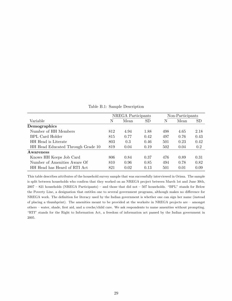
Table B.1: Sample Description

NREGA Participants Non-Participants

Variable N Mean SD N Mean SD

DemographicsNumber of HH Members 812 4.94 1.88 498 4.65 2.18BPL Card Holder 815 0.77 0.42 497 0.76 0.43HH Head is Literate 803 0.3 0.46 501 0.23 0.42HH Head Educated Through Grade 10 819 0.04 0.19 502 0.04 0.2

AwarenessKnows HH Keeps Job Card 806 0.84 0.37 476 0.89 0.31Number of Amenities Aware Of 810 0.96 0.85 494 0.78 0.82HH Head has Heard of RTI Act 821 0.02 0.13 501 0.01 0.09

This table describes attributes of the household survey sample that was successfully interviewed in Orissa. The sample

is split between households who confirm that they worked on an NREGA project between March 1st and June 30th,

2007 – 821 households (NREGA Participants) – and those that did not – 507 households. “BPL” stands for Below

the Poverty Line, a designation that entitles one to several government programs, although makes no difference for

NREGA work. The definition for literacy used by the Indian government is whether one can sign her name (instead

of placing a thumbprint). The amenities meant to be provided at the worksite in NREGA projects are – amongst

others – water, shade, first aid, and a creche/child care. We ask respondents to name amenities without prompting.

“RTI” stands for the Right to Information Act, a freedom of information act passed by the Indian government in

2005.

29

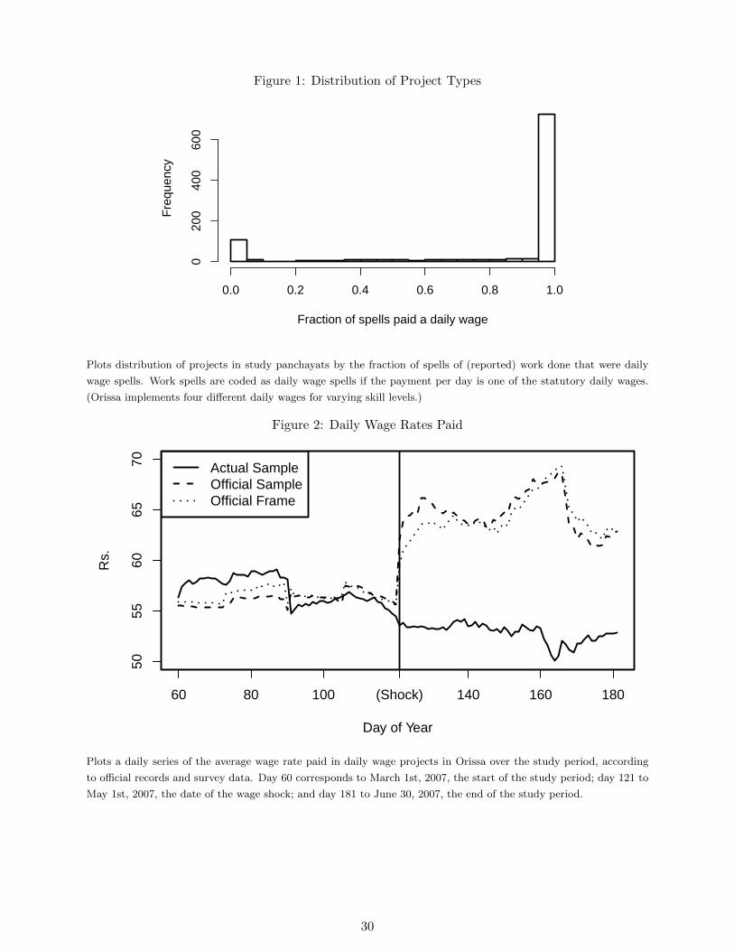
Figure 1: Distribution of Project TypesDistribution of Project Types

Fraction of spells paid a daily wage

Fre

quen

cy

0.0 0.2 0.4 0.6 0.8 1.0

020

040

060

0

Plots distribution of projects in study panchayats by the fraction of spells of (reported) work done that were daily

wage spells. Work spells are coded as daily wage spells if the payment per day is one of the statutory daily wages.

(Orissa implements four different daily wages for varying skill levels.)

Figure 2: Daily Wage Rates Paid

5055

6065

70

Day of Year

Rs.

Actual SampleOfficial SampleOfficial Frame

60 80 100 140 160 180(Shock)

Plots a daily series of the average wage rate paid in daily wage projects in Orissa over the study period, according

to official records and survey data. Day 60 corresponds to March 1st, 2007, the start of the study period; day 121 to

May 1st, 2007, the date of the wage shock; and day 181 to June 30, 2007, the end of the study period.

30

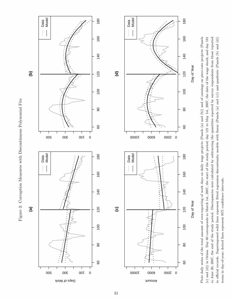
Fig

ure

3:C

orru

pti

onM

easu

res

wit

hD

isco

nti

nu

ous

Pol

yn

omia

lF

its

6080

100

120

140

160

180

0100300500(a

)

Days of Work

Dat

aM

odel

6080

100

120

140

160

180

0100300500

(b)

Dat

aM

odel

6080

100

120

140

160

180

02000600010000

(c)

Day

of Y

ear

Amount

Dat

aM

odel

6080

100

120

140

160

180

02000600010000

(d)

Day

of Y

ear

Dat

aM

odel

Plo

tsdaily

seri

esof

the

tota

lam

ount

of

over

-rep

ort

ing

of

work

day

son

daily

wage

pro

ject

s(P

anel

s(a

)and

(b))

and

of

earn

ings

on

pie

ce-r

ate

pro

ject

s(P

anel

s

(c)

and

(d))

inO

riss

a.

Day

60

corr

esp

onds

toM

arc

h1st

,2007,

the

start

of

the

study

per

iod;

day

121

toM

ay1st

,2007,

the

date

of

the

wage

shock

;and

day

181

toJune

30,

2007,

the

end

of

the

study

per

iod.

Dis

crep

anci

esw

ere

calc

ula

ted

by

subtr

act

ing

the

quanti

ties

rep

ort

edby

surv

eyre

sponden

tsfr

om

those

rep

ort

ed

inoffi

cial

reco

rds.

Sup

erim

pose

dso

lid

lines

repre

sent

fitt

edre

gre

ssio

ndis

conti

nuit

ym

odel

sw

ith

linea

r(P

anel

s(a

)and

(c))

and

quadra

tic

(Panel

s(b

)and

(d))

term

sin

day

-of-

yea

r;dott

edlines

repre

sent

95%

confiden

cein

terv

als

.

31

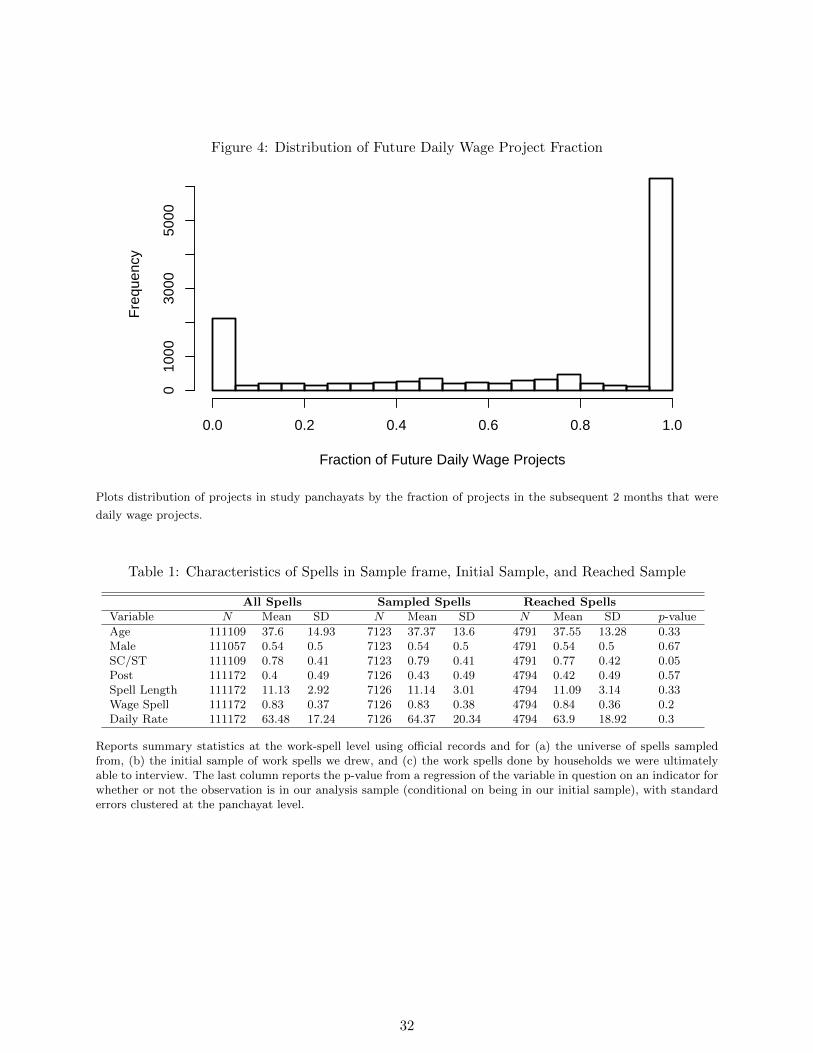
Figure 4: Distribution of Future Daily Wage Project Fraction

Fraction of Future Daily Wage Projects

Fre

quen

cy

0.0 0.2 0.4 0.6 0.8 1.0

010

0030

0050

00

Plots distribution of projects in study panchayats by the fraction of projects in the subsequent 2 months that were

daily wage projects.

Table 1: Characteristics of Spells in Sample frame, Initial Sample, and Reached Sample

All Spells Sampled Spells Reached SpellsVariable N Mean SD N Mean SD N Mean SD p-value

Age 111109 37.6 14.93 7123 37.37 13.6 4791 37.55 13.28 0.33Male 111057 0.54 0.5 7123 0.54 0.5 4791 0.54 0.5 0.67SC/ST 111109 0.78 0.41 7123 0.79 0.41 4791 0.77 0.42 0.05Post 111172 0.4 0.49 7126 0.43 0.49 4794 0.42 0.49 0.57Spell Length 111172 11.13 2.92 7126 11.14 3.01 4794 11.09 3.14 0.33Wage Spell 111172 0.83 0.37 7126 0.83 0.38 4794 0.84 0.36 0.2Daily Rate 111172 63.48 17.24 7126 64.37 20.34 4794 63.9 18.92 0.3

Reports summary statistics at the work-spell level using official records and for (a) the universe of spells sampledfrom, (b) the initial sample of work spells we drew, and (c) the work spells done by households we were ultimatelyable to interview. The last column reports the p-value from a regression of the variable in question on an indicator forwhether or not the observation is in our analysis sample (conditional on being in our initial sample), with standarderrors clustered at the panchayat level.

32

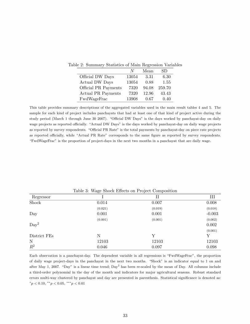
Table 2: Summary Statistics of Main Regression Variables

N Mean SD

Official DW Days 13054 3.31 6.30Actual DW Days 13054 0.88 1.55Official PR Payments 7320 94.08 259.70Actual PR Payments 7320 12.96 43.43FwdWageFrac 13908 0.67 0.40

This table provides summary descriptions of the aggregated variables used in the main result tables 4 and 5. The

sample for each kind of project includes panchayats that had at least one of that kind of project active during the

study period (March 1 through June 30 2007). “Official DW Days” is the days worked by panchayat-day on daily

wage projects as reported officially. “Actual DW Days” is the days worked by panchayat-day on daily wage projects

as reported by survey respondents. “Official PR Rate” is the total payments by panchayat-day on piece rate projects

as reported officially, while “Actual PR Rate” corresponds to the same figure as reported by survey respondents.

“FwdWageFrac” is the proportion of project-days in the next two months in a panchayat that are daily wage.

Table 3: Wage Shock Effects on Project Composition

Regressor I II III

Shock 0.014 0.007 0.008(0.021) (0.019) (0.018)

Day 0.001 0.001 -0.003(0.001) (0.001) (0.002)

Day2 0.002(0.001)

District FEs N Y YN 12103 12103 12103R2 0.046 0.097 0.098

Each observation is a panchayat-day. The dependent variable in all regressions is “FwdWageFrac”, the proportion

of daily wage project-days in the panchayat in the next two months. “Shock” is an indicator equal to 1 on and

after May 1, 2007. “Day” is a linear time trend; Day2 has been re-scaled by the mean of Day. All columns include

a third-order polynomial in the day of the month and indicators for major agricultural seasons. Robust standard

errors multi-way clustered by panchayat and day are presented in parenthesis. Statistical significance is denoted as:∗p < 0.10, ∗∗p < 0.05, ∗∗∗p < 0.01

33

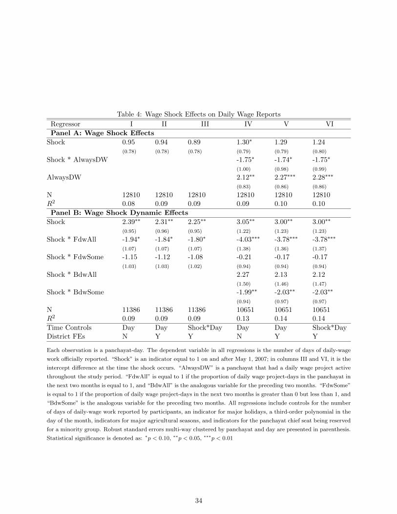
Table 4: Wage Shock Effects on Daily Wage Reports

Regressor I II III IV V VI

Panel A: Wage Shock Effects

Shock 0.95 0.94 0.89 1.30∗ 1.29 1.24(0.78) (0.78) (0.78) (0.79) (0.79) (0.80)

Shock * AlwaysDW -1.75∗ -1.74∗ -1.75∗

(1.00) (0.98) (0.99)

AlwaysDW 2.12∗∗ 2.27∗∗∗ 2.28∗∗∗

(0.83) (0.86) (0.86)

N 12810 12810 12810 12810 12810 12810R2 0.08 0.09 0.09 0.09 0.10 0.10

Panel B: Wage Shock Dynamic Effects

Shock 2.39∗∗ 2.31∗∗ 2.25∗∗ 3.05∗∗ 3.00∗∗ 3.00∗∗

(0.95) (0.96) (0.95) (1.22) (1.23) (1.23)

Shock * FdwAll -1.94∗ -1.84∗ -1.80∗ -4.03∗∗∗ -3.78∗∗∗ -3.78∗∗∗

(1.07) (1.07) (1.07) (1.38) (1.36) (1.37)

Shock * FdwSome -1.15 -1.12 -1.08 -0.21 -0.17 -0.17(1.03) (1.03) (1.02) (0.94) (0.94) (0.94)

Shock * BdwAll 2.27 2.13 2.12(1.50) (1.46) (1.47)

Shock * BdwSome -1.99∗∗ -2.03∗∗ -2.03∗∗

(0.94) (0.97) (0.97)

N 11386 11386 11386 10651 10651 10651R2 0.09 0.09 0.09 0.13 0.14 0.14

Time Controls Day Day Shock*Day Day Day Shock*DayDistrict FEs N Y Y N Y Y

Each observation is a panchayat-day. The dependent variable in all regressions is the number of days of daily-wage

work officially reported. “Shock” is an indicator equal to 1 on and after May 1, 2007; in columns III and VI, it is the

intercept difference at the time the shock occurs. “AlwaysDW” is a panchayat that had a daily wage project active

throughout the study period. “FdwAll” is equal to 1 if the proportion of daily wage project-days in the panchayat in

the next two months is equal to 1, and “BdwAll” is the analogous variable for the preceding two months. “FdwSome”

is equal to 1 if the proportion of daily wage project-days in the next two months is greater than 0 but less than 1, and

“BdwSome” is the analogous variable for the preceding two months. All regressions include controls for the number

of days of daily-wage work reported by participants, an indicator for major holidays, a third-order polynomial in the

day of the month, indicators for major agricultural seasons, and indicators for the panchayat chief seat being reserved

for a minority group. Robust standard errors multi-way clustered by panchayat and day are presented in parenthesis.

Statistical significance is denoted as: ∗p < 0.10, ∗∗p < 0.05, ∗∗∗p < 0.01

34

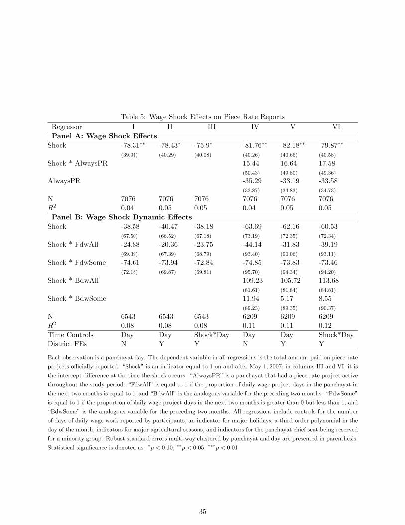
Table 5: Wage Shock Effects on Piece Rate Reports

Regressor I II III IV V VI

Panel A: Wage Shock Effects

Shock -78.31∗∗ -78.43∗ -75.9∗ -81.76∗∗ -82.18∗∗ -79.87∗∗

(39.91) (40.29) (40.08) (40.26) (40.66) (40.58)

Shock * AlwaysPR 15.44 16.64 17.58(50.43) (49.80) (49.36)

AlwaysPR -35.29 -33.19 -33.58(33.87) (34.83) (34.73)

N 7076 7076 7076 7076 7076 7076R2 0.04 0.05 0.05 0.04 0.05 0.05

Panel B: Wage Shock Dynamic Effects

Shock -38.58 -40.47 -38.18 -63.69 -62.16 -60.53(67.50) (66.52) (67.18) (73.19) (72.35) (72.34)

Shock * FdwAll -24.88 -20.36 -23.75 -44.14 -31.83 -39.19(69.39) (67.39) (68.79) (93.40) (90.06) (93.11)

Shock * FdwSome -74.61 -73.94 -72.84 -74.85 -73.83 -73.46(72.18) (69.87) (69.81) (95.70) (94.34) (94.20)

Shock * BdwAll 109.23 105.72 113.68(81.61) (81.84) (84.81)

Shock * BdwSome 11.94 5.17 8.55(89.23) (89.35) (90.37)

N 6543 6543 6543 6209 6209 6209R2 0.08 0.08 0.08 0.11 0.11 0.12

Time Controls Day Day Shock*Day Day Day Shock*DayDistrict FEs N Y Y N Y Y

Each observation is a panchayat-day. The dependent variable in all regressions is the total amount paid on piece-rate

projects officially reported. “Shock” is an indicator equal to 1 on and after May 1, 2007; in columns III and VI, it is

the intercept difference at the time the shock occurs. “AlwaysPR” is a panchayat that had a piece rate project active

throughout the study period. “FdwAll” is equal to 1 if the proportion of daily wage project-days in the panchayat in

the next two months is equal to 1, and “BdwAll” is the analogous variable for the preceding two months. “FdwSome”

is equal to 1 if the proportion of daily wage project-days in the next two months is greater than 0 but less than 1, and

“BdwSome” is the analogous variable for the preceding two months. All regressions include controls for the number

of days of daily-wage work reported by participants, an indicator for major holidays, a third-order polynomial in the

day of the month, indicators for major agricultural seasons, and indicators for the panchayat chief seat being reserved

for a minority group. Robust standard errors multi-way clustered by panchayat and day are presented in parenthesis.

Statistical significance is denoted as: ∗p < 0.10, ∗∗p < 0.05, ∗∗∗p < 0.01

35

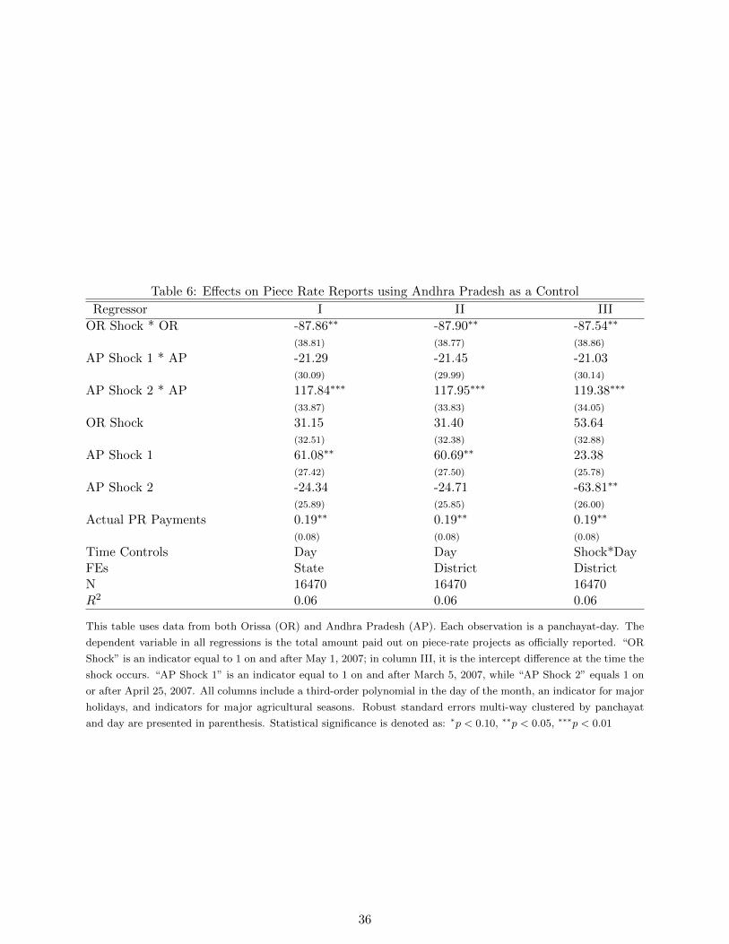
Table 6: Effects on Piece Rate Reports using Andhra Pradesh as a Control

Regressor I II III

OR Shock * OR -87.86∗∗ -87.90∗∗ -87.54∗∗

(38.81) (38.77) (38.86)

AP Shock 1 * AP -21.29 -21.45 -21.03(30.09) (29.99) (30.14)

AP Shock 2 * AP 117.84∗∗∗ 117.95∗∗∗ 119.38∗∗∗

(33.87) (33.83) (34.05)

OR Shock 31.15 31.40 53.64(32.51) (32.38) (32.88)

AP Shock 1 61.08∗∗ 60.69∗∗ 23.38(27.42) (27.50) (25.78)

AP Shock 2 -24.34 -24.71 -63.81∗∗

(25.89) (25.85) (26.00)

Actual PR Payments 0.19∗∗ 0.19∗∗ 0.19∗∗

(0.08) (0.08) (0.08)

Time Controls Day Day Shock*DayFEs State District DistrictN 16470 16470 16470R2 0.06 0.06 0.06

This table uses data from both Orissa (OR) and Andhra Pradesh (AP). Each observation is a panchayat-day. The

dependent variable in all regressions is the total amount paid out on piece-rate projects as officially reported. “OR

Shock” is an indicator equal to 1 on and after May 1, 2007; in column III, it is the intercept difference at the time the

shock occurs. “AP Shock 1” is an indicator equal to 1 on and after March 5, 2007, while “AP Shock 2” equals 1 on

or after April 25, 2007. All columns include a third-order polynomial in the day of the month, an indicator for major

holidays, and indicators for major agricultural seasons. Robust standard errors multi-way clustered by panchayat

and day are presented in parenthesis. Statistical significance is denoted as: ∗p < 0.10, ∗∗p < 0.05, ∗∗∗p < 0.01

36

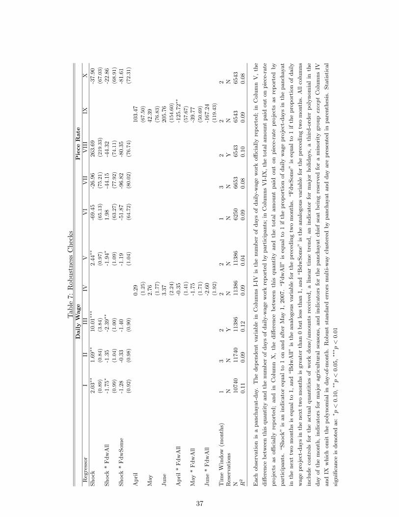
Tab

le7:

Rob

ust

nes

sC

hec

ks

Daily

Wage

PieceRate

Reg

ress

or

III

III

IVV

VI

VII

VII

IIX

X

Shock

2.0

3∗∗

1.6

9∗∗

10.0

1∗∗∗

2.4

4∗∗

-69.4

5-2

6.9

6263.6

9-3

7.9

0(0.89)

(0.84)

(3.84)

(0.97)

(65.13)

(75.21)

(219.33)

(67.03)

Shock

*F

dw

All

-1.7

5∗

-1.3

5-2

.39∗∗

-1.9

4∗

1.9

8-4

4.1

5-4

4.3

2-2

2.8

6(0.99)

(1.04)

(1.00)

(1.09)

(63.27)

(77.92)

(74.11)

(68.91)

Shock

*F

dw

Som

e-1

.28

-0.3

3-1

.40

-1.1

9-5

1.8

7-9

6.8

2-8

0.3

5-8

1.6

1(0.92)

(0.98)

(0.90)

(1.04)

(64.72)

(80.02)

(76.74)

(72.31)

Apri

l0.2

9103.4

7(1.25)

(67.50)

May

2.7

642.3

9(1.77)

(76.83)

June

3.3

7205.7

6(2.24)

(154.60)

Apri

l*

Fdw

All

-0.3

5-1

25.7

2∗∗

(1.41)

(57.67)

May

*F

dw

All

-1.7

5-3

9.7

7(1.71)

(50.69)

June

*F

dw

All

-2.6

0-1

67.2

4(1.92)

(119.43)

Tim

eW

indow

(month

s)1

32

22

13

22

2R

eser

vati

ons

NN

YN

NN

NY

NN

N10740

11740

11386

11386

11386

6250

6653

6543

6543

6543

R2

0.1

10.0

90.1

20.0

90.0

40.0

90.0

80.1

00.0

90.0

8

Each

obse

rvati

on

isa

panch

ayat-

day

.T

he

dep

enden

tva

riable

inC

olu

mns

I-IV

isth

enum

ber

of

day

sof

daily-w

age

work

offi

cially

rep

ort

ed;

inC

olu

mn

V,

the

diff

eren

ceb

etw

een

this

quanti

tyand

the

num

ber

of

day

sof

daily-w

age

work

rep

ort

edby

part

icip

ants

;in

Colu

mns

VI-

IX,

the

tota

lam

ount

paid

out

on

pie

ce-r

ate

pro

ject

sas

offi

cially

rep

ort

ed;

and

inC

olu

mn

X,

the

diff

eren

ceb

etw

een

this

quanti

tyand

the

tota

lam

ount

paid

out

on

pie

ce-r

ate

pro

ject

sas

rep

ort

edby

part

icip

ants

.“Shock

”is

an

indic

ato

req

ual

to1

on

and

aft

erM

ay1,

2007.

“F

dw

All”

iseq

ual

to1

ifth

epro

port

ion

of

daily

wage

pro

ject

-day

sin

the

panch

ayat

inth

enex

ttw

om

onth

sis

equal

to1,

and

“B

dw

All”

isth

eanalo

gous

vari

able

for

the

pre

cedin

gtw

om

onth

s.“F

dw

Som

e”is

equal

to1

ifth

epro

port

ion

of

daily

wage

pro

ject

-day

sin

the

nex

ttw

om

onth

sis

gre

ate

rth

an

0but

less

than

1,

and

“B

dw

Som

e”is

the

analo

gous

vari

able

for

the

pre

cedin

gtw

om

onth

s.A

llco

lum

ns

incl

ude

contr

ols

for

the

act

ual

quanti

ties

of

work

done/

am

ounts

rece

ived

,a

linea

rti

me

tren

d,

an

indic

ato

rfo

rm

ajo

rholiday

s,a

thir

d-o

rder

poly

nom

ial

inth

e

day

of

the

month

,in

dic

ato

rsfo

rm

ajo

ragri

cult

ura

lse

aso

ns,

and

indic

ato

rsfo

rth

epanch

ayat

chie

fse

at

bei

ng

rese

rved

for

am

inori

tygro

upexcept

Colu

mns

IV

and

IXw

hic

hom

itth

ep

oly

nom

ial

inday

-of-

month

.R

obust

standard

erro

rsm

ult

i-w

aycl

ust

ered

by

panch

ayat

and

day

are

pre

sente

din

pare

nth

esis

.Sta

tist

ical

signifi

cance

isden

ote

das:∗p<

0.1

0,∗∗p<

0.0

5,∗∗∗p<

0.0

1

37

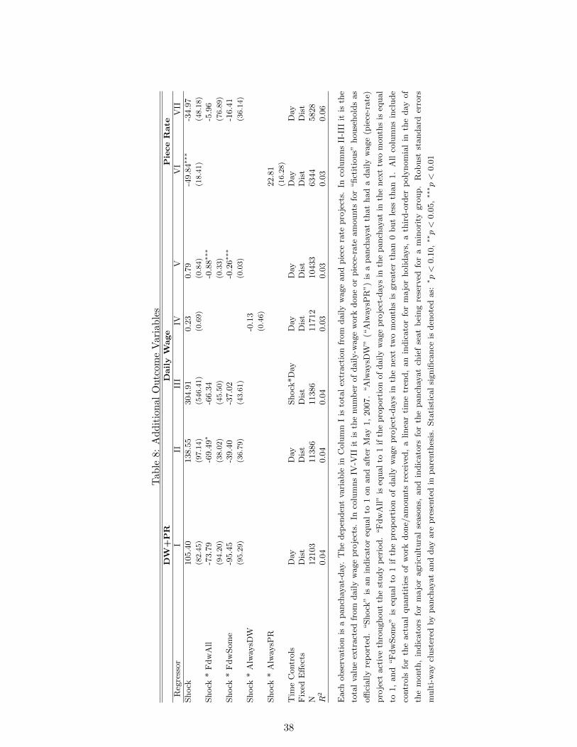
Tab

le8:

Ad

dit

ion

alO

utc

ome

Var

iab

les

DW

+PR

Daily

Wage

PieceRate

Reg

ress

or

III

III

IVV

VI

VII

Shock

105.4

0138.5

5304.9

10.2

30.7

9-4

9.8

4∗∗∗

-34.9

7(82.45)

(97.14)

(546.41)

(0.69)

(0.84)

(18.41)

(48.18)

Shock

*F

dw

All

-73.7

9-6

9.4

9∗

-66.3

4-0

.88∗∗∗

-5.9

6(94.20)

(38.02)

(45.50)

(0.33)

(76.89)

Shock

*F

dw

Som

e-9

5.4

5-3

9.4

0-3

7.0

2-0

.26∗∗∗

-16.4

1(95.29)

(36.79)

(43.61)

(0.03)

(36.14)

Shock

*A

lway

sDW

-0.1

3(0.46)

Shock

*A

lway

sPR

22.8

1(16.28)

Tim

eC

ontr

ols

Day

Day

Shock

*D

ayD

ayD

ayD

ayD

ayF

ixed

Eff

ects

Dis

tD

ist

Dis

tD

ist

Dis

tD

ist

Dis

tN

12103

11386

11386

11712

10433

6344

5828

R2

0.0

40.0

40.0

40.0

30.0

30.0

30.0

6

Each

obse

rvati

on

isa

panch

ayat-

day

.T

he

dep

enden

tva

riable

inC

olu

mn

Iis

tota

lex

tract

ion

from

daily

wage

and

pie

cera

tepro

ject

s.In

colu

mns

II-I

IIit

isth

e

tota

lva

lue

extr

act

edfr

om

daily

wage

pro

ject

s.In

colu

mns

IV-V

IIit

isth

enum

ber

of

daily-w

age

work

done

or

pie

ce-r

ate

am

ounts

for

“fict

itio

us”

house

hold

sas

offi

cially

rep

ort

ed.

“Shock

”is

an

indic

ato

req

ual

to1

on

and

aft

erM

ay1,

2007.

“A

lway

sDW

”(“

Alw

aysP

R”)

isa

panch

ayat

that

had

adaily

wage

(pie

ce-r

ate

)

pro

ject

act

ive

thro

ughout

the

study

per

iod.

“F

dw

All”

iseq

ual

to1

ifth

epro

port

ion

of

daily

wage

pro

ject

-day

sin

the

panch

ayat

inth

enex

ttw

om

onth

sis

equal

to1,

and

“F

dw

Som

e”is

equal

to1

ifth

epro

port

ion

of

daily

wage

pro

ject

-day

sin

the

nex

ttw

om

onth

sis

gre

ate

rth

an

0but

less

than

1.

All

colu

mns

incl

ude

contr

ols

for

the

act

ual

quanti

ties

of

work

done/

am

ounts

rece

ived

,a

linea

rti

me

tren

d,

an

indic

ato

rfo

rm

ajo

rholiday

s,a

thir

d-o

rder

poly

nom

ial

inth

eday

of

the

month

,in

dic

ato

rsfo

rm

ajo

ragri

cult

ura

lse

aso

ns,

and

indic

ato

rsfo

rth

epanch

ayat

chie

fse

at

bei

ng

rese

rved

for

am

inori

tygro

up.

Robust

standard

erro

rs

mult

i-w

aycl

ust

ered

by

panch

ayat

and

day

are

pre

sente

din

pare

nth

esis

.Sta

tist

ical

signifi

cance

isden

ote

das:∗p<

0.1

0,∗∗p<

0.0

5,∗∗∗p<

0.0

1

38

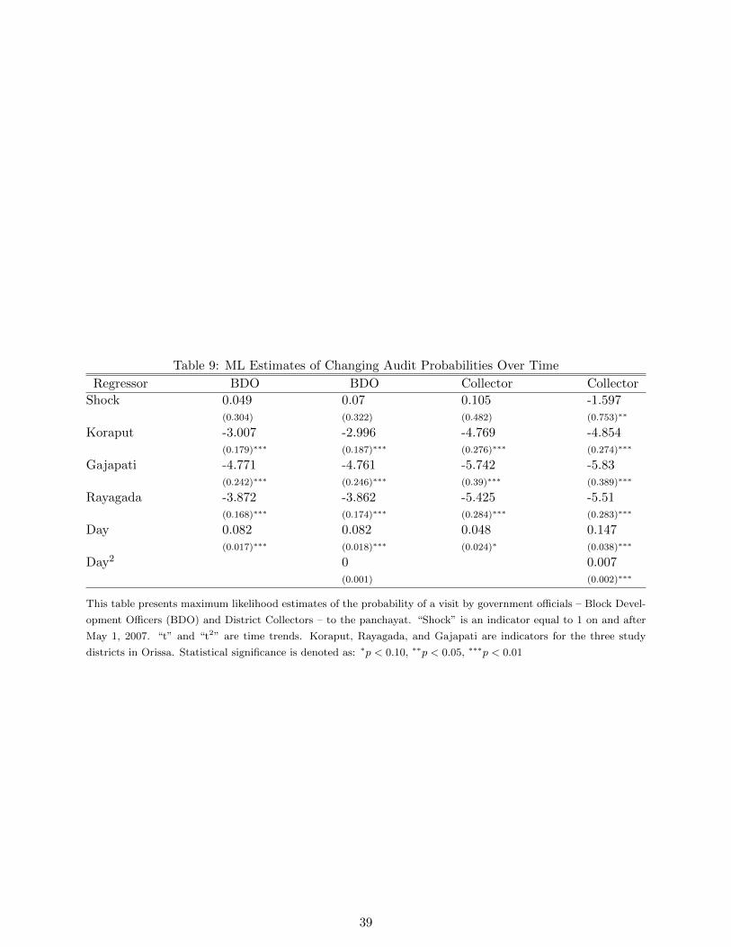
Table 9: ML Estimates of Changing Audit Probabilities Over Time

Regressor BDO BDO Collector Collector

Shock 0.049 0.07 0.105 -1.597(0.304) (0.322) (0.482) (0.753)∗∗

Koraput -3.007 -2.996 -4.769 -4.854(0.179)∗∗∗ (0.187)∗∗∗ (0.276)∗∗∗ (0.274)∗∗∗

Gajapati -4.771 -4.761 -5.742 -5.83(0.242)∗∗∗ (0.246)∗∗∗ (0.39)∗∗∗ (0.389)∗∗∗

Rayagada -3.872 -3.862 -5.425 -5.51(0.168)∗∗∗ (0.174)∗∗∗ (0.284)∗∗∗ (0.283)∗∗∗

Day 0.082 0.082 0.048 0.147(0.017)∗∗∗ (0.018)∗∗∗ (0.024)∗ (0.038)∗∗∗

Day2 0 0.007(0.001) (0.002)∗∗∗

This table presents maximum likelihood estimates of the probability of a visit by government officials – Block Devel-

opment Officers (BDO) and District Collectors – to the panchayat. “Shock” is an indicator equal to 1 on and after

May 1, 2007. “t” and “t2” are time trends. Koraput, Rayagada, and Gajapati are indicators for the three study

districts in Orissa. Statistical significance is denoted as: ∗p < 0.10, ∗∗p < 0.05, ∗∗∗p < 0.01

39

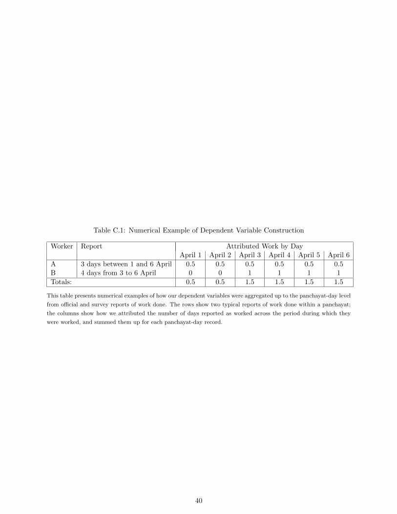
Table C.1: Numerical Example of Dependent Variable Construction

Worker Report Attributed Work by DayApril 1 April 2 April 3 April 4 April 5 April 6

A 3 days between 1 and 6 April 0.5 0.5 0.5 0.5 0.5 0.5B 4 days from 3 to 6 April 0 0 1 1 1 1

Totals: 0.5 0.5 1.5 1.5 1.5 1.5

This table presents numerical examples of how our dependent variables were aggregated up to the panchayat-day level

from official and survey reports of work done. The rows show two typical reports of work done within a panchayat;

the columns show how we attributed the number of days reported as worked across the period during which they

were worked, and summed them up for each panchayat-day record.

40

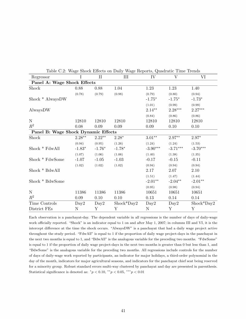
Table C.2: Wage Shock Effects on Daily Wage Reports, Quadratic Time Trends

Regressor I II III IV V VI

Panel A: Wage Shock Effects

Shock 0.88 0.88 1.04 1.23 1.23 1.40(0.78) (0.79) (0.98) (0.79) (0.80) (0.94)

Shock * AlwaysDW -1.75∗ -1.75∗ -1.73∗

(1.01) (0.99) (0.99)

AlwaysDW 2.14∗∗ 2.28∗∗∗ 2.27∗∗∗

(0.84) (0.86) (0.86)

N 12810 12810 12810 12810 12810 12810R2 0.08 0.09 0.09 0.09 0.10 0.10

Panel B: Wage Shock Dynamic Effects

Shock 2.28∗∗ 2.22∗∗ 2.28∗ 3.01∗∗ 2.97∗∗ 2.97∗

(0.94) (0.95) (1.26) (1.24) (1.24) (1.53)

Shock * FdwAll -1.83∗ -1.76∗ -1.78∗ -3.90∗∗∗ -3.71∗∗∗ -3.70∗∗∗

(1.07) (1.06) (1.06) (1.40) (1.38) (1.35)

Shock * FdwSome -1.07 -1.05 -1.03 -0.17 -0.15 -0.11(1.02) (1.02) (1.02) (0.94) (0.94) (0.94)

Shock * BdwAll 2.17 2.07 2.10(1.51) (1.47) (1.44)

Shock * BdwSome -2.01∗∗ -2.04∗∗ -2.01∗∗

(0.95) (0.98) (0.94)

N 11386 11386 11386 10651 10651 10651R2 0.09 0.10 0.10 0.13 0.14 0.14

Time Controls Day2 Day2 Shock*Day2 Day2 Day2 Shock*Day2District FEs N Y Y N Y Y

Each observation is a panchayat-day. The dependent variable in all regressions is the number of days of daily-wage

work officially reported. “Shock” is an indicator equal to 1 on and after May 1, 2007; in columns III and VI, it is the

intercept difference at the time the shock occurs. “AlwaysDW” is a panchayat that had a daily wage project active

throughout the study period. “FdwAll” is equal to 1 if the proportion of daily wage project-days in the panchayat in

the next two months is equal to 1, and “BdwAll” is the analogous variable for the preceding two months. “FdwSome”

is equal to 1 if the proportion of daily wage project-days in the next two months is greater than 0 but less than 1, and

“BdwSome” is the analogous variable for the preceding two months. All regressions include controls for the number

of days of daily-wage work reported by participants, an indicator for major holidays, a third-order polynomial in the

day of the month, indicators for major agricultural seasons, and indicators for the panchayat chief seat being reserved

for a minority group. Robust standard errors multi-way clustered by panchayat and day are presented in parenthesis.

Statistical significance is denoted as: ∗p < 0.10, ∗∗p < 0.05, ∗∗∗p < 0.01

41

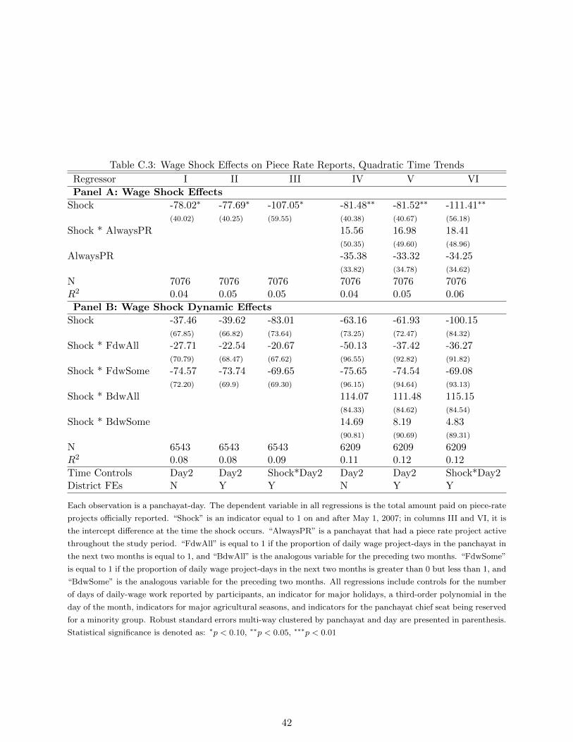
Table C.3: Wage Shock Effects on Piece Rate Reports, Quadratic Time Trends

Regressor I II III IV V VI

Panel A: Wage Shock Effects

Shock -78.02∗ -77.69∗ -107.05∗ -81.48∗∗ -81.52∗∗ -111.41∗∗

(40.02) (40.25) (59.55) (40.38) (40.67) (56.18)

Shock * AlwaysPR 15.56 16.98 18.41(50.35) (49.60) (48.96)

AlwaysPR -35.38 -33.32 -34.25(33.82) (34.78) (34.62)

N 7076 7076 7076 7076 7076 7076R2 0.04 0.05 0.05 0.04 0.05 0.06

Panel B: Wage Shock Dynamic Effects

Shock -37.46 -39.62 -83.01 -63.16 -61.93 -100.15(67.85) (66.82) (73.64) (73.25) (72.47) (84.32)

Shock * FdwAll -27.71 -22.54 -20.67 -50.13 -37.42 -36.27(70.79) (68.47) (67.62) (96.55) (92.82) (91.82)

Shock * FdwSome -74.57 -73.74 -69.65 -75.65 -74.54 -69.08(72.20) (69.9) (69.30) (96.15) (94.64) (93.13)

Shock * BdwAll 114.07 111.48 115.15(84.33) (84.62) (84.54)

Shock * BdwSome 14.69 8.19 4.83(90.81) (90.69) (89.31)

N 6543 6543 6543 6209 6209 6209R2 0.08 0.08 0.09 0.11 0.12 0.12

Time Controls Day2 Day2 Shock*Day2 Day2 Day2 Shock*Day2District FEs N Y Y N Y Y

Each observation is a panchayat-day. The dependent variable in all regressions is the total amount paid on piece-rate

projects officially reported. “Shock” is an indicator equal to 1 on and after May 1, 2007; in columns III and VI, it is

the intercept difference at the time the shock occurs. “AlwaysPR” is a panchayat that had a piece rate project active

throughout the study period. “FdwAll” is equal to 1 if the proportion of daily wage project-days in the panchayat in

the next two months is equal to 1, and “BdwAll” is the analogous variable for the preceding two months. “FdwSome”

is equal to 1 if the proportion of daily wage project-days in the next two months is greater than 0 but less than 1, and

“BdwSome” is the analogous variable for the preceding two months. All regressions include controls for the number

of days of daily-wage work reported by participants, an indicator for major holidays, a third-order polynomial in the

day of the month, indicators for major agricultural seasons, and indicators for the panchayat chief seat being reserved

for a minority group. Robust standard errors multi-way clustered by panchayat and day are presented in parenthesis.

Statistical significance is denoted as: ∗p < 0.10, ∗∗p < 0.05, ∗∗∗p < 0.01

42

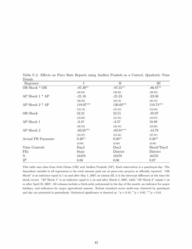
Table C.4: Effects on Piece Rate Reports using Andhra Pradesh as a Control, Quadratic TimeTrendsRegressor I II III

OR Shock * OR -87.39∗∗ -87.31∗∗ -86.87∗∗

(38.94) (38.92) (38.93)

AP Shock 1 * AP -21.10 -21.24 -23.30(30.29) (30.18) (30.18)

AP Shock 2 * AP 119.97∗∗∗ 120.03∗∗∗ 119.74∗∗∗

(34.13) (34.10) (34.08)

OR Shock 52.21 52.51 -35.07(32.00) (31.94) (43.97)

AP Shock 1 -3.47 -3.57 18.89(26.52) (26.43) (22.00)

AP Shock 2 -63.85∗∗∗ -63.91∗∗∗ -44.79(24.27) (24.22) (27.81)

Actual PR Payments 0.20∗∗ 0.20∗∗ 0.20∗∗

(0.08) (0.08) (0.08)

Time Controls Day2 Day2 Shock*Day2FEs State District DistrictN 16470 16470 16470R2 0.06 0.06 0.07

This table uses data from both Orissa (OR) and Andhra Pradesh (AP). Each observation is a panchayat-day. The

dependent variable in all regressions is the total amount paid out on piece-rate projects as officially reported. “OR

Shock” is an indicator equal to 1 on and after May 1, 2007; in column III, it is the intercept difference at the time the

shock occurs. “AP Shock 1” is an indicator equal to 1 on and after March 5, 2007, while “AP Shock 2” equals 1 on

or after April 25, 2007. All columns include a third-order polynomial in the day of the month, an indicator for major

holidays, and indicators for major agricultural seasons. Robust standard errors multi-way clustered by panchayat

and day are presented in parenthesis. Statistical significance is denoted as: ∗p < 0.10, ∗∗p < 0.05, ∗∗∗p < 0.01

43