Corruption and Retrospective DemocraticAccountability

Brian F. CrispJoshua D. PotterSantiago OlivellaWilliam Mishler

December 2011

Abstract

Many theories of democracy stress the concept of accountability. Voters reward orpunish elected officials by extending or ending their political careers. This retrospectiveprincipal/agent relationship is supposed to induce good behavior on the part of electedofficials. Seeking the long-term reward of reelection, officials avoid the short-termbenefits of corruption that would put them at risk of early electoral defeat. However,if voters frequently change their allegiances, making political careers typically short,incentives to refrain from malfeasance are reduced and accountability undermined. Thissuggests that punishing politicians perceived to be corrupt may not diminish futuremalfeasance. To test this possibility, we employ a bivariate normal model to assessthe reciprocal effects of electoral volatility on corruption and, conversely, corruptionon electoral volatility. We test the hypothesized relationship on data drawn from 249elections across 74 countries. Our results show that corruption does indeed provokeelectoral volatility but that volatility has no discernible impact on malfeasance – or onvirtuous behavior, for that matter.1

1We would like to thank Benjamin Bricker, Adriana Crespo Tenorio, Jeff Gill, Nate Jensen, AndrewMartin, James Monogan, Jacob Montgomery, Guillermo Rosas, and Margit Tavits for helpful comments onprevious drafts of this paper. We also thank John Golightly for his assistance with data collection.

1 Introduction

In Federalist no. 57, Madison wrote that “the aim of every political constitution is . . . first

to obtain for rulers men who possess most wisdom to discern, and most virtue to pursue, the

common good of society, and in the next place, to take the most effectual precautions for

keeping them virtuous whilst they continue to hold their public trust.” Putting Madison’s

aim into action, voters seek both to choose “good” representatives and to provide incentives

for them to remain virtuous after they have been elected (Przeworski, Stokes and Manin,

1999). Those incentives follow from voters’ willingness to remove from office at the next

election anyone who failed to represent them well, including those suspected of corrupt

practices. Indeed, Riker argues that it is more accurate from what he calls the “Madisonian”

or “liberal ideal” to conceive of the vote as a negative check on underperforming politicians

rather than as the collective expression of the electorate’s future policy preferences (Riker,

1982).

In most democracies, politicians are at least partly reelection seekers. Their desire to ex-

tend their careers – and voters’ control over that extension – is supposed to keep politicians

on their best behavior. Representatives who pursue self-enrichment over the public good

give voters good reason to transfer their support to other candidates, thereby ending the

incumbents’ careers and reinforcing the incentive for their replacements to behave better.

As a result, politicians avoid malfeasance and other acts likely to alienate voters (Cohen

and Spitzer, 1996; Carey, 2003; Alt and Dreyer Lassen, 2003; Spiller, Stein and Tommasi,

2008). A theory of Retrospective Accountability therefore posits the existence of a virtuous

cycle. Voters respond to malfeasance by “throwing the bums out.” This display of electoral

volatility replaces the bums with more virtuous representatives, who having seen retrospec-

tive accountability in action, remain virtuous so as not to evoke another spate of volatility.

As a result, corruption declines, virtuous representatives get re-elected, and political corrup-

tion and electoral volatility dwindle in tandem – a virtuous cycle ends in a state of good

government.

2

Retrospective accountability assumes that elected officials have long time horizons. How-

ever, if politicians do not have reasonable prospects for long careers, the electoral incentives

for them to behave virtuously are diminished. A problem for retrospective accountability

is that elected officials may be be voted out of office – and their time horizons shortened

– for a variety of reasons, including malfeasance. Rival politicians may convince voters

that incumbents are corrupt even when they are not. Exogenous shocks, such as an eco-

nomic crisis, may lead voters to punish incumbents even if the shocks were unavoidable

(Powell and Whitten, 1993; Anderson, 2000). A new policy dimension might be introduced

– whether inadvertently by a crisis or intentionally by political rivals – thereby dividing

groups in the electorate along new axes that result in a drop in support for incumbents

(Chhibber and Torcal, 1997). Inexperienced or unsophisticated voters (perhaps recently

after the (re)establishment of democratic rule) may be uncertain of their options or their

preferences over them (Bielasiak, 2002; Tavits and Annus, 2006). For all these reasons –

as well as the possibility that actually corrupt politicians will be perceived as such – where

electoral volatility is high, incumbents may reasonably decide that they cannot expect a long

career even if they behave virtuously. In such an environment, elected representatives may

conclude that a rational response to the vagaries of re-election is to seek short-term gains,

including self-enrichment.

Rather than serving as a check on corruption, retrospective democratic accountability

could, then, contribute to a vicious cycle in which voters repeatedly vote officials out of

office for any number of different reasons including but not limited to corruption. This elec-

toral volatility shortens future politicians’ perceived time horizons. In turn, shortened time

horizons make self-enrichment more rational, leading to still more volatility in the name of

holding politicians accountable. Thus, rather than a virtuous cycle leading to an equilibrium

characterized by stable voting patterns and generally good government, efforts at account-

ability could create a steady state of high electoral volatility and continuing malfeasance.

We seek to better understand the relationship between retrospective accountability and

3

the quality of representation by testing for a reciprocal relationship between electoral volatil-

ity and political corruption. We begin by developing more fully our theoretical motivation

regarding the relationship between legislators’ expectations about their time horizons (which

we measure with electoral volatility) and their decisions about whether or not to engage in

corrupt practices (which we measure with citizens’ perceptions of legislative corruption). We

then estimate Vector Auto Regression (VAR) models using data on electoral volatility and

perceived corruption for 249 elections in 74 countries. We find that as theories of retrospec-

tive democratic accountability would predict, where voters perceive politicians to be corrupt,

they take their electoral support elsewhere, increasing electoral volatility. However, levels of

electoral volatility have no effect on perceived corruption. In other words, neither a virtuous

or a vicious cycle exists and corruption is impervious to electoral punishment. We conclude

by situating our findings in the broader literature on retrospective voting and democratic

accountability.

2 Time Horizons and Malfeasance

Przeworski, Stokes and Manin (1999) maintain that “[g]overnments are ‘accountable’ if cit-

izens can discern representative from unrepresentative governments and can sanction them

appropriately, retaining in office those incumbents who perform well and ousting from office

those who do not. . . . . Elections are a contingent renewal accountability mechanism,

where the sanctions are to extend or not to extend the government’s tenure” (10). Thus,

key to democratic accountability is the chance to retrospectively evaluate the performance

of incumbents (Fiorina, 1981; Lewis-Beck and Stegmaier, 2000). Positive evaluations lead

to reelection through preference stability on the part of voters. Negative evaluations lead to

defeat through the electoral volatility resulting from changing voter preferences.

Accountability is necessary because there are many reasons why elected officials may

behave in ways contrary to voters’ preferences. Politicians may misunderstand those prefer-

4

ences or have contrary preferences of their own, leading them to enact policies that voters

dislike. The loss of representative agency suffered by voters depends on how far government

policy is placed from the voter’s ideal point in a a policy space. Another way in which politi-

cians’ behavior can be costly to voters is if politicians place their own welfare over that of the

voters’. A politician’s welfare may include spending time competing with rivals, engaging

in clientelistic practices to the benefit of family and friends, and/or increasing his or her

own personal wealth. Given the many reasons why politicians’ behavior may not comport

with the preferences of voters, being able to exercise retrospective accountability is a key

component of democratic practice.

Much of the literature on economic voting has at its heart an understanding of voting

as the practice of retrospective accountability (Powell and Whitten, 1993; Kiewit, 2000).

Voters assess the state of the economy and make a decision about whether the incumbent

government should be rewarded with reelection. Debates continue about how much detail

voters need (and have) about economic conditions (Lohmann, 1999; Anderson and O’Connor,

2000); the role of clarity of responsibility for vote choice (Tavits, 2007); and whether assess-

ments are based on the voters’ personal conditions or on general conditions (Lewis-Beck and

Stegmaier, 2000). However, common to both sides of every debate is the characterization of

voting as an opportunity to get rid of incumbents who have failed to represent the voters’

interests – in other words, to “throw the bums out,” presumably bringing to office politicians

who will be on their best behavior or suffer the same fate. Where the new politicians behave

better and are rewarded with reelection, a virtuous cycle has been put in place.

Equally central to democratic theory is politicians’ desire for reelection and their belief

that good, representative behavior on their part makes reelection likely. Where this is the

case, voters control something politicians want – their vote – and politicians know what

strategy to adopt – good behavior – to get it (Carey, 1998). The idea that politicians

value reelection assumes, inter alia, that politicians perceive greater long-term benefits to

themselves from remaining in office as compared to the short-term benefits of grabbing all

5

that they can for themselves before the voters turn them out after a single, corrupt term. If

elected officials know they cannot be re-elected – as for example where they are term limited

– or if they discount the long term benefits of office, the effects of electoral accountability

are undermined. Indeed, in the study of term limits across U.S. state legislatures, there

is empirical evidence to suggest that, for example, limits fundamentally reshape sitting

legislators’ policy priorities (Gurwitt, 1996; Hansen, 1997) and that they also undermine

the extent to which individual legislators are responsive to their specific constituency (Carey

et al., 2006; Carey, 1994; Zupan, 1990). Like imposed limits on career length, it is possible

that throwing the bums out too frequently sends perverse signals to elected officials that they

should hurry up and be bums while the opportunity presents itself (Besley and Case, 1995;

Alt and Dreyer Lassen, 2003). Short time horizons have been shown to lead to perverse,

instrumental behaviors in a variety of settings. Many game theoretic outcomes are based

on the assumptions that play is iterative and that the players do not know when play will

end (Fudenberg and Maskin, 1986). Often, when the end of play is known, chances for

cooperative or virtuous behavior disappear as by backward logic both players decide to

defect in the initial round.

As Spiller, Stein and Tommasi (2008) note: “it is not the same to have a legislature

in which the same individuals interact repeatedly over extended periods of time as it is to

have a legislature where individual legislators are frequently replaced” (18). While primarily

concerned with cooperative relationships among politicians, their thinking on the effects of

short time horizons applies to the relationship between politicians and voters too. Longer

time horizons lead to lower discount rates, meaning politicians will place greater value on the

accomplishments they can achieve by being virtuous representatives and staying in power as

compared to more immediate payoffs, including those that might end their careers. Where

politicians do not believe they will have the opportunity to earn voters’ trust, and thereby

extend their careers, their short time horizon makes bad behavior, including perhaps engag-

ing in corruption, the option with the greatest payoff. Cross-national tests of this logic have

6

yet to be conducted, but a recent empirical investigation of Brazilian municipal elections is

telling. Ferraz and Finan (2011) construct their own objective measure of corruption from

audit reports attached to local government electoral contests and find that there exists a sig-

nificant difference in corruption levels between municipalities where mayors can get reelected

and those where they cannot.

To determine whether the relationship between political corruption and electoral volatility

is virtuous or vicious requires testing these simple, interrelated hypotheses:

• H1: Higher levels of corruption by legislators induces higher levels of electoral volatility.

• H2A: If the relationship is virtuous, higher levels of electoral volatility, in turn, inducesubsequently lower levels of corruption by legislators.

• H2B: If the relationship is vicious, higher levels of electoral volatility, in turn, inducesubsequently higher levels of corruption by legislators.

In sum, the retrospective voting dynamic tells us that an important part of democratic

rule is punishing politicians who have behaved badly by voting for someone else who will

behave better. By contrast, the time horizon dynamic tells us that if politicians expect to

be thrown out of office, they will seek short-term payoffs, including self-enrichment through

corruption. Taken together, we have either a virtuous or vicious feedback cycle: voters

punish politicians for bad behavior, including malfeasance, and politicians decide to engage

in good practices because they want to increase the probability of long careers or voters

punish politicians for bad behavior, including malfeasance, and politicians decide to engage

in corrupt practices because they discount the probability of long careers given the volatile

electorate.

3 Data

By definition, corruption is illegal. Those engaged in the practice go to great lengths to

conceal their behavior. Not surprisingly, it has proven very challenging to develop objective

7

measures of corruption (Treisman, 2007). Because we are interested in citizens’ judgments

regarding the conduct of elected representatives, however, objective measures of corruption

are less central to our theorizing than citizen perceptions of that corruption, however ac-

curate or inaccurate those perceptions might be. While the World Bank and Transparency

International publish well known measures of perceived corruption, there most used mea-

sures are based primarily on the perceptions of country experts, not citizens. Moreover,

those measures reflect the level of corruption in a country as a whole and do not distinguish

levels of corruption in different institutions.

Since 2004, Transparency International has collected annual survey data on citizens’

perceptions of corruption in a broad, and growing, cross-section of countries. The Global

Corruption Barometer (GCB) asks citizens their perceptions of corruption not only for the

government sector as a whole but for a variety of more specific institutions, including the

national legislature, the judiciary, and various branches of the bureaucracy. Given our focus

on efforts to exercise retrospective accountability over elected officials, we use the the GCB

question that asks citizens: “To what extent do you perceive the parliament/legislature in

this country to be affected by corruption?”2 Responses were recorded on a five-point scale

ranging from “not at all corrupt” (1) to “extremely corrupt” (5). The GCB reports the

country average (mean) responese on this scale. So, the aggregated variable, practically

speaking, is a continuous variable with values between 1 and 5.

Treisman (2007) – among others – has raised concerns about the extent to which subjec-

tive survey measures of corruption can be safely assumed to approximate an objective (but

directly unmeasurable) level of corruption. He points out, however, that the global percep-

tions indices managed by Transparency International and the World Bank actually correlated

rather highly with more objective (but, from a cross-national perspective, comparatively lim-

ited in scope) measures of self-reported corruption experiences. Indeed, when individuals and

2The responses to this question were correlated at r = 0.92 with the responses to an identical questionasking about corruption of political parties.

8

business managers are asked whether their families or companies have paid governing offi-

cials bribes, their responses correlated highly with what the surveys reveal about corruption

perceptions (Treisman, 2007). Furthermore, Treisman notes that the GCB’s battery of ques-

tions about perceptions related specifically to the political sphere correlate highly with the

larger, country-level perceptions of corruption captured by TI and WB. Whether the survey

responses of citizens capture a latent objective level of corruption variable or not (Lambs-

dorff, 2004; Treisman, 2007), they are ideal for our purposes given that it is perceptions that

inform vote choice.

Due to the fact that our causal reasoning rests on the assumption that a country’s

democratic institutions are at least functional, we include in the analysis only those countries

that are at least partially democratic. However, we were also concerned that if we selected

only perfectly healthy and well-developed democracies we would run the risk of ending up

with a dataset full of cases across which corruption does not vary. Conventional wisdom led

us to suspect that better performing democracies would, virtually by definition, have lower

levels of corruption (Treisman, 2000, 2007; Montinola and Jackman, 2002; Brunetti and

Weder, 2003; Adsera, Boix and Payne, 2003). As a result, we chose to focus on democratic

regimes identified with a fairly permissive inclusion criterion (however, our concern was

misplaced, with results holding under a more restrictive case selection criteria).3 For all of

the countries covered by the GCB, we collected Freedom House data from the year 2000 to

2010. If a particular country scored a “Free” or “Partly Free” designation in more than 75%

of its observations, we include it in our study.4 The resulting set of countries – broken down

by geographic region – is included in Appendix A at the end of this manuscript. In the end,

we collected corruption data for 74 democratic regimes from around the world.

In the process of collecting data on electoral volatility, we sought vote distributions

3When we subset our data to include only democracies with a polity score greater than 7, we get thesame susbstantive results we report below, though model fit is slightly worse because the residuals are notbivariate normally distributed.

4We dropped an additional eight countries from this initial group due to the unavailability of electoralvote data.

9

amongst parties at the national level in each country starting two elections prior to 2004

(the first year of the GCB corruption data). This allowed us, in most cases, to calculate one

observation of electoral volatility prior to the first observation of corruption perceptions.5

Our electoral data come from a variety of sources. For most elections in Europe and other

OECD countries, we drew from the online European Elections Database which is provided

by the National University of Ireland. For elections in Africa, we relied on the online African

Elections Database, which is an aggregator of electoral data garnered from electoral author-

ities in each country on the African continent. For many elections in Latin America and

Asia and a few elections in Europe, we drew data from the electoral handbook series edited

by Dieter Nohlen (Nohlen, 2005; Nohlen, Grotz and Hartmann, 2001; Nohlen and Stover,

2010). The remaining balance of electoral data was taken directly from electoral commissions

in each respective country.6

Taagepera and Grofman (2003) evaluate several indices of disproportionality and inter-

election volatility and conclude that the Pedersen Index (Pedersen, 1983) and the Gallagher

Index (Gallagher, 1991) “satisfy more criteria than any other” in terms of their ability to

capture the dynamics of electoral volatility (p. 673). For the observations in our data set, the

two indexes produce volatility figures that are highly correlated with one another (r = 0.94).

We estimate our models with the Pedersen Index, which is mathematically defined as :

Pedersen =1

2

N∑i=1

|pi,t − pi,t−1|

Where pi,t is party i’s vote share at time t and pi,t−1 is party i’s vote share at time t− 1.7

5We chose to focus on volatility in votes rather than seats. This has the advantage of picking up on subtlechanges in the electorate’s preferences that, while registered in vote fluctuations, might not be registered inseat fluctuations. Practically speaking, however, the choice between the two is generally immaterial as voteand seat volatility tend to be very highly correlated.

6Even the most thorough electoral data repositories typically group votes for very unpopular parties intoan “other” category, thereby slightly compromising the ability to calculate precisely the level of volatility.Fortunately, for the country-years in our data set, the average proportion of the vote in the “other parties”category was less than 3.7%.

7Reasoning that perhaps politicians only reformed their behavior when they saw votes going to entirely

10

In order to evaluate the proposed relationship between our variables of interest – elec-

toral volatility and perceived legislative corruption, we need to keep track of the temporal

nuances involved in using each series both in explanatory and outcome roles. In general,

only temporally antecedent values of each series should be used to predict current states of

the other phenomenon and, whenever possible, both series should be composed of measure-

ments generated at the same intervals. For our series, it is usually the case that corruption

measures come in shorter intervals than our measures of volatility, because the surveys on

which the former are based are not constrained to election years. For this reason, we take

the inter-election period as our unit of analysis, and generate values of political corruption

at the appropriate level of aggregation by averaging all corruption measurements that may

have been obtained in the years between elections, excluding measurements taken on election

years themselves. As a result, each observation is composed of two values – one of the elec-

toral volatility observed in the year that maks the beggining of the inter election period, and

one of political corruption observed throughout the years strictly between elections. Finally,

and in order to keep track of different countries in our samples, the series’ lagged values are

constructed within countries, in order to avoid allowing previous values of a different country

to help predict current values of another.8

We now turn to our statistical analysis of the two dynamics described above: the ret-

rospective voting dynamic that is a hallmark assumption of the normative desirability of

democratic representation and the time horizon dynamic which potentially poses a challenge

new parties, we measured volatility based solely on this dynamic (what Tucker and Powell (2010) refer toas “Volatility A”). Using just new party volatility, we get the same susbstantive results we report below,though, again, model fit is slightly worse because the residuals are not bivariate normally distributed.

8When trying to establish the simultaneous effects of phenomena over time, the literature often reliesexclusively on the predictive power of the time trends of the phenomena of interest. As a result, models ofthese dynamics often lack the types of statistical controls common to other modeling techniques, focusingon the joint significance of self and cross lagged values of the endogenous variables of interest. We followthis practice in the model we discuss and present in the next section (for other examples of this, see Brandtand Jones, 2006; Enders and Sandler, 1993; Edwards and Wood, 1999). Nothing in the theory of vectorautoregressions precludes the inclusion of exogenous variables, however, and their use may even be desirablein order to rule out spuriousness. Consequently, Appendix C presents the results of a model estimationwhich includes a battery of exogenous variables.

11

to this classic conceptualization of democratic representation. If retrospective accountability

is working as theorized, we should find that corruption leads voters to switch votes and that

corruption declines as future politicians heed the warning. To the contrary, if a perverse

cycle exists, corruption may generate electoral volatility but that volatility will lead to more

corruption as politicians with short time horizons behave selfishly.

4 Analysis

Testing our hypotheses is akin to establishing whether (1) electoral volatility can be better

predicted when a temporally antecedent value of political corruption is used for generat-

ing the prediction; (2) the same is true about political corruption with respect to electoral

volatility; (3) it is the case that larger values of temporally preceding corruption are expected

to increase the values of subsequent volatility; and (4) it is the case that larger values of

the temporally preceding volatility are expected to decrease values of subsequent corruption

(if a virtuous relationship exists) or increase the values of subsequent corruption (if a vi-

cious relationship exists). Either way, the mechanism we propose generates a feedback, or

simultaneity relationship, between corruption and electoral volatility.

A common modeling strategy to account for this type of simultaneous relationship con-

sists of using structural equations (Freeman, Williams and Lin, 1989). In general, instru-

ments are incorporated in a two-stage estimation process in order to ‘purge’ presumably

endogenous variables from the variation that is attributed to the very phenomenon they are

expected to affect. In practice, finding appropriate instruments is problematic. In order for

the instrumental variables approach to yield correct estimates of the hypothesized relation-

ship, instruments must both (1) have a non-zero effect on the instrumented phenomenon

and (2) be unrelated to the explained variable once the instrumented phenomenon is taken

into account (Angrist, Imbens and Rubin, 1993). Because verifying the latter – the so-called

exclusion restriction – is inherently difficult in an empirical setting, the validity of the results

12

obtained through this procedure hinge on an assumption that often leads to inconclusive and

contradictory results (Freeman, Williams and Lin, 1989).

A modeling alternative which circumvents these potential problems is vector autoregres-

sion (VAR) – a technique that generalizes autoregressive models (i.e. models of time series

that make current states a function of the series’ historic trend) to enable simultaneous anal-

ysis of multiple, interdependent series. By relaxing the need to know the specific functional

form relating the two endogenous phenomena, VAR models are able to produce estimates of

the general, historic dependency between them. Hence, although VAR models restrict our

ability to directly test the specific mechanism through which two phenomena are caught in

an interdependency, they allow us to establish whether the proposed feedback relationship

is actually present, when relevant conditions are met9 (Freeman, Williams and Lin, 1989;

Freeman et al., 1998). For instance, a VAR model of order 1 (i.e. a model in which a single

lag of each of two series are used to predict their current values) would be defined by:

yt = c +

φ12 γ12

γ21 φ21

y1,t−1

y2,t−1

+ u (1)

where c is a vector of constants, u is a vector of residuals drawn from a bivariate dis-

tribution (usually a bivariate Normal with a a zero mean vector and an identity covariance

matrix), the φ’s are self-lag coefficients and the γ’s are cross-lag coefficients (i.e. coefficients

corresponding to lags of on series we hypothesize is causing the other series).

VAR models are especially well suited for evaluating Granger causality, which is said

to exist between phenomena Y and X if their future is better predicted when accounting

for both the history of X and of Y , rather than simply the trend of either one by itself

9More specifically when the series being evaluated are either stationary or, in case they are not, coin-tegrated. Substantively, these conditions insure that we can infer something generalizable about the seriesunder study by using their observed behavior. For a detailed explanation of what these two conditions entail,see Hamilton (1994)

13

(Freeman, 1983).10 When including the appropriate number of self-lags as predictors, VAR

models provide the most natural direct test of Granger causality between any number of

time series.11

As a result, these models are ideal for testing theories that pose the existence of a feedback

relationship that occurs over time – such as the one we have posed between electoral volatility

and legislative corruption. Figure ?? depicts the way in which the modeling strategy works

for the bivariate VAR model defined above. The dotted lines represent the effects we are

interested in (e.g. in our case the effects of corruption on volatility and vice versa), whereas

the solid lines represent the impact of a series’ immediate history on its current value. In a

sense, then, the VAR model allows us to gauge each series’ effect on the other after filtering

out the explained series’ historic trend.

[Insert Figure 1 About Here]

We implement such a VAR model of order 112 to test whether there is a Granger feed-

back between electoral volatility and political corruption. In order to obtain estimates of

our model’s coefficients and of their distributions we use MCMC simulations. In general,

Bayesian estimation techniques of VAR models are particularly useful for the purpose at

hand because they provide a direct sample of the actual posterior sampling distributions

of coefficients, even in the face of non-stationary time series. The model assumes that the

10To be precise, when it is the case that the future of Y can be better predicted by past values of X and Ythan by values of Y alone, it is said that X Granger-causes Y . Similarly, when the same can be said aboutX with respect to Y , it is said that Y Granger-causes X, establishing a Granger feedback between X andY .

11Examples of political science works that evaluate Granger causality abound (see, for instance, Edwardsand Wood, 1999; Enders and Sandler, 1993; Hartley and Russett, 1992; MacKuen, Erikson and Stimson,1992).

12Direct tests of Granger causality require an inclusion of as many self-lags as needed to eliminate serialautocorrelations of any order. Although we cannot test all possible orders of autocorrelation, we are confidentthat the two self-lags we include in our model are sufficient to control for the predictive power of eachvariable’s historic trend for both theoretical (volatility that is far removed in the past should not affectcurrent electoral volatility) and empirical (See Figure 1 in Appendix B, which plots the autocorrelationfunctions for the residuals for each of the estimated equations; the included lags eliminate any trace of serialcorrelation of any order) reasons.

14

phenomena of interest (viz. electoral volatility and legislative corruption at any given leg-

islative term) are random draws from a bivariate normal distribution, the elements of the

mean vector of which are functions of a constant term; one self-lag and one cross-lag (with

variables constructed in the manner described in the previous section). As a result, the

model is exactly as that defined in Equation 1 above. The model further estimates the

(contemporaneous) correlation between the two phenomena of interest, thereby relaxing the

assumption of independence of residuals across the two processes. Finally, to better acco-

modate normality and to allow for possible non-linearities, we estimate our model using the

log of electoral volatility.13 For more details on the estimation procedure, see Appendix B.

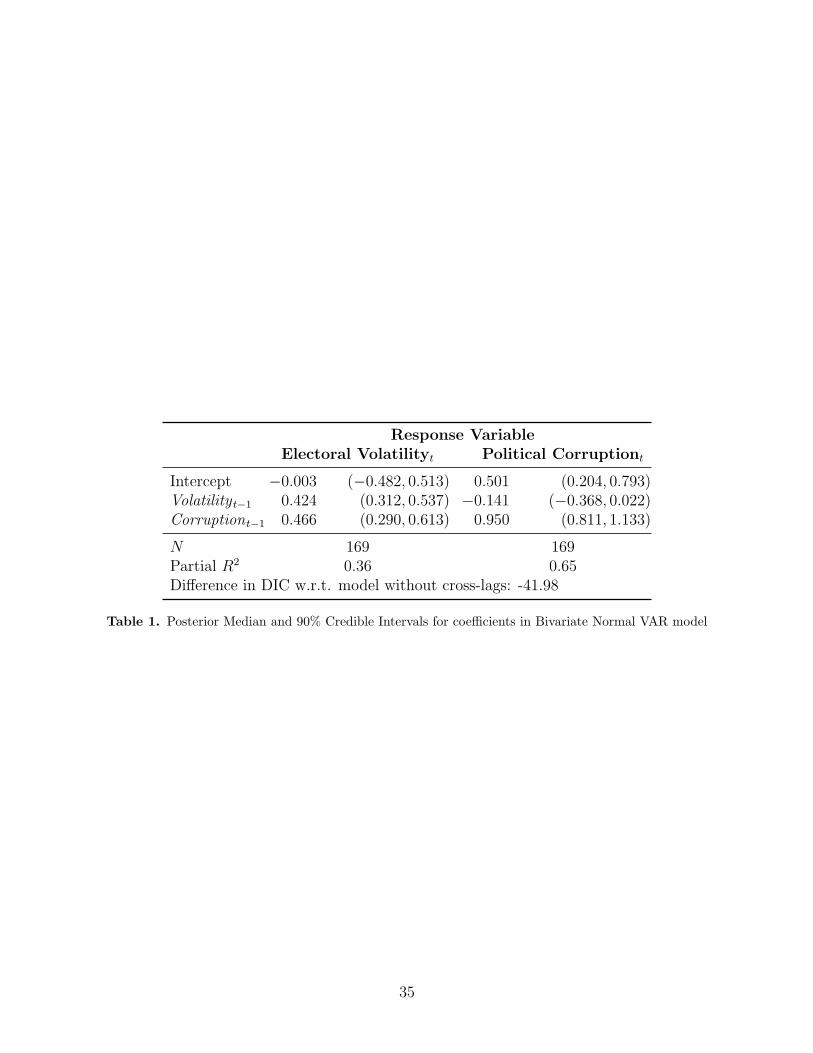
The results of the estimation are presented in Table 2, which reports the observed medians

of the sampled posterior distributions of estimated parameters along with their 0.05 and

0.95 quantiles. We use these summary statistics as our point estimates and our 90% credible

intervals, respectively.

[Insert Table 2 About Here]

The bivariate normal model is a good fit for the data. Although partial R2 measures

are relatively low (0.36 and 0.65 for the volatility and corruption equations, respectively),

residuals are distributed bivariate-normally around the zero vector (we fail to reject the

null hypothesis of a Shapiro-Wilk test of multivariate normality with a p-value of 0.18) and

all serial autocorrelation appears to be accounted for by the specified model, justifying the

number of lags chosen (see Appendix B for a plot of the autocorrelation function for the

residuals of each equation). The modeling strategy is further justified by the fact that the

probability that the ρ coefficient is positive and different from zero is greater than 0.70: the

posterior median for ρ is estimated to be 0.256, with a 70% credible interval between 0.023

and 0.459.

The sizable (viz. -41.98) difference in deviances suggests that the model using a single

cross-lag for predicting each series provides a much better fit of the data than a model that

13something about why this is substantively justifiable too

15

includes only self lags. Results presented in Table 2, however, indicate that Granger causality

can only be reliably posited when considering the effect of corruption on electoral volatility

(left column). In support of hypothesis 1, the probability that increasing immediately past

perceptions of corruption leads to greater electoral volatility is high (i.e. greater than 0.9):

voters are therefore likely to express their discontent in the face of high perceived corrup-

tion by expressing preferences for different alternatives.14 More specifically, Figure 2 shows

predicted values (as 90% highest posterior density intervals for each prediction) of electoral

volatility at time t for different levels of perceived corruption at time t − 1, holding the

immediate past level of volatility constant at its observed average. The predicted values can

be construed as the effects of an exogenously achieved level of perceived corruption on future

levels of electoral volatility. Our model predicts that exogenously increasing perceptions of

corruption from 1.7 to 4.8 (the variable’s observed range) can result in a dramatic increase

in volatility – from 8 to almost 36% volatility.

[Insert Figure 2 About Here]

Our cross-national test of H1 generates confirmatory findings; in other words, across the

countries included in our study, we can see that citizens respond to increases in perceived

corruption by swinging their electoral support to different parties. We can see this trend

borne out in individual countries as well. Consider the case of Lithuania. In the lead up

to the 2004 election and 2008 elections, incumbent politicians in Lithuanian were beset by

corruption scandals (Velykis, 2010). The GCB report scored Lithuania at 4.2 on a 5-point

scale leading up to the 2004 election and at 4.0 leading up to the 2008 election. In both

14Tucker and Powell (2010) note that electoral volatility can result from two potentially distinct processes:parties entering and exiting electoral races (Type A volatility) and voters casting votes for different, butpreexisting, alternatives (Type B volatility). These types of electoral volatility may express different things(for instance, Type A volatility is more clearly the result of party-elite entry decisions than of shifting voterpreferences), and they may generate different types of incentives for politicians (for instance, time horizonsmay be perceived to be shorter when volatility is of Type A than of Type B, because the latter could generatea sort of repeated game amongst old political players). As a result, we estimated our model using measuresof Type A and Type B volatility instead of the overall volatility measure we have reported. All resultsremain substantively the same: although corruption Granger-causes volatility, volatility does not appear toGranger cause corruption.

16

cases, the Lithuanian people responded to these high profile corruption cases by voting

for the opposition parties (Lithuania: Constitution and Institutions, 2007; Country Report:

Lithuania (2008), N.d.). Indeed, total volatility figures in these elections were 86.2 and

65.1, respectively. These figures are much larger than one standard deviation above the

mean volatility score for our cross-national data set. Additionally, theses figures specifically

reflect Lithuanian’s acute sense of disappointment in persisting levels of corruption (Velykis,

2010). In national electoral surveys in 2008, for example, half of respondents indicated that

both the parliament and the government were “very corrupt” entities and, furthermore, 83%

responded that these national politicians should be held more responsible for the level of

corruption.

By contrast to the test of H1, however, the evidence in Table 2 and Figure 2 does

not support either version of Hypothesis 2. The absence of any causal effect of electoral

volatility on perceived corruption is inconsistent with the Retrospective Voting dynamic

(H2A), which predicts a negative influence of volatility on corruption producing a virtuous

circle in which replacement legislators are chastened to behave virtuously thereby reducing

future volatility. It also is inconsistent with the Time Horizon dynamic (H2B) which predicts

a positive influence of volatility of corruption contributing to a vicious circle of ever increasing

corruption and volatility. The absence of any impact of volatility on perceived corruption

means either that legislators do not alter their behavior in the short run in response to the

incentives (positive or negative) provided by vote volatility, or that politicians do respond,

but their change in behavior is not immediately perceived by voters who continue to punish

newly elected legislators for the sins of their predecessors. The very strong, lagged effect in

Table 2 of perceived corruption on itself (.967) is consistent with both possibilities.

Distinguishing between these possibilities, empirically, requires data on actual legislative

corruption, which is not available. Nevertheless, as between the two the second is more

plausible. Voter perceptions of legislative corruption appear highly viscous; they do not vary

much over time. Corruption is covert and hard for voters to recognize. When they do perceive

17

corruption, voters respond appropriately by throwing the bums out of office. But because

corruption is covert, it is equally difficult for voters to know if newly elected legislators are

really better behaved or whether the corruption of new members simply has not been exposed

yet. In the absence of visible evidence to the contrary, voters have no reason to update their

perceptions and treat the new legislators any differently than the old ones. Rather than

creating either a virtuous or a vicious circle, this creates instead a low-level equilibrium trap.

Voter perceptions of corruption give rise to higher levels of volatility, but because higher

volatility has no impact on subsequent perceptions of corruption, continuing perceptions

of corruption are likely to sustain those higher levels of volatility, thereby threatening the

re-election prospects of newly elected legislators regardless of their behavior.

The results of the cross-national statistical analysis evaluating H2 affirm what we know

of several individual countries around the world: if volatility does not incentivize more

corruption, it at least fails to curb it. Consider the case of Israel, which between 2004 and

2010 averaged a 4.35 on the GCBs 5-point scale of citizen perceptions about the extent of

corruption in political parties. There were three parliamentary elections during this time

period with volatility figures of 49.1 in 2003, 74.2 in 2006, and 43.5 in 2009. While the spike in

volatility in 2006 can be partially attributed to the emergence of the new Kadima Party, the

persistent level of volatility reflects voters sustained dissatisfaction with the corrupt practices

of elected politicians. Galia Sagy, the Head of Transparency International in Israel, argues

that the string of public prosecutions of corrupt politicians in Israel conveys information

to the voters about the overall level of corruption in the political system (Dattel, 2011).

She notes a direct tie between voters perceptions about corruption and the accrual of legal

cases against national-level politicians (Dattel, 2011). There is also reason to believe that

these perceptions are, in turn, informing vote choice. Certainly this was the case in 1977,

when corruption charges forced Prime Minister Yitzhak Rabin to close down his campaign

and prompted voters to move their support away from the Labor Party and toward more

right-leaning parties (Benn, 2009). It has also been the case in more recent years, where

18

Ehud Olmert, anticipating dire reelection prospects, specifically cited corruption accusations

in his announcement that he would not run in his partys primary in 2008 (Olmert, 2008).

Despite his admission that his corrupt practices were shaping his electoral prospects, however,

electoral volatility has done little to actually curtail corruption in Israel. In 2010, citizen

perception of corruption in political parties was at 4.5 among the highest levels in the world.

The same holds true in Bosnia-Herzegovina. A very high level of perceived corruption

in 2005 (4.5) prompted a 123% increased in total volatility between 2002 (20.4) and 2006

(45.5). Despite the upswing in volatility, it does not appearing that politicians were get-

ting the message, as subsequent measures of perceived corruption in 2005 and 2007 showed

the figure holding steady at 4.5 and 4.4, respectively. Transparency Internationals National

Integrity System Study for Bosnia-Herzegovina in 2007 notes that perceptions of corrup-

tion in the country were being driven mainly by “critically problematic pillars in society

such as political parties and “the highest levels of elected office (Transparency-International,

2007). While the 2006 election was a highly salient election for a number of reasons, we

have good cause to suspect that citizens were also concerned about the extent of corruption

among national politicians. A survey conducted by the World Bank in 2000 concludes that

there was “a high level of public concern regarding corruption with citizens believing that

corruption was responsible for greater inequality, higher crime rates, and reduced foreign in-

vestment (World-Bank, 2000). Furthermore, more than 97% of survey respondents indicated

that corruption “leads to very serious consequences for their country (World-Bank, 2000).

Despite the fact that citizens in Bosnia-Herzegovina both (1) identified national politicians

specifically as the source of corruption and (2) indicated that corruption was a driving is-

sue in the countrys politics, their efforts at curbing corruption were ineffective. Of the 163

countries ranked by the Global Perceptions Index on a yearly basis, Bosnia-Herzegovina

fell from 70th place in 2003, to tied for 88th place in 2005, to tied for 98th place in 2006

(Transparency-International, 2007).

In summary, both cross-national and anecdotal evidence seems to suggest that, although

19

more corruption is expected to lead to more electoral volatility, increasing volatility does

not seem to have any effect on the level of corruption. As a result, then, the more general

case for classical democratic accountability is still found wanting: ousting corrupt politicians

from office, while not setting off a vicious spiral, does not seem to have the normative effect

accountability theory would suggest it should have.

5 Discussion and Conclusion

We began this paper by raising concerns about the standard theory of Retrospective Ac-

countability on which the logic of Representative Government heavily depends. According

to the standard theory, voters hold elected officials accountable for their performance in

office by voting out of office anyone suspected of corrupt behavior. This presumably purges

government of the worst officials, reminds continuing representatives of the voters’ power,

and signals newly elected officials to behave more virtuously than their predecessors. We

argued, however, that the standard theory hinges on the assumption that elected officials

have long time horizons such that they can reasonably conclude that the long-term benefits

of remaining virtuous in office exceed the short term benefits of corruption. Our concern

with the standard theory is simply that where electoral volatility or turnover is high, for

whatever reasons, the time horizons of elected officials should shrink, thereby decreasing the

incentives for good behavior.

The evidence we have reported is reassuring of the standard model in several respects.

It clearly shows, for example, that voters respond appropriately to perceived corruption by

throwing legislators out of office. The data reported also provide reassurance regarding the

time horizons of elected officials in that we do not find any evidence that increasing electoral

volatility results in greater corruption or a vicious cycle. Nevertheless, the observation

that increasing volatility does not reduce corruption undermines a central assumption of

Retrospective Accountability theory: namely, that the replacement of corrupt officials creates

20

a virtuous cycle where corruption and volatility are mutually reinforcing and spiral ever lower

together.

We do not wish to overstate our findings. Ours is but the latest contribution to a long

history of research on Retrospective Accountability. The results, based as they are on a

relatively small number of countries over a relatively short period of time, certainly require

replication and refinement. One question that needs to be addressed is whether there is

something unique about political corruption that makes it different from other forms of

malfeasance. Whereas corruption is typically covert and hard to perceive, other legislative

behaviors are transparent. A legislator who signs a no-new-taxes pledge and reneges by

voting for tax increases does so in full public view as do legislators who fail to introduce or

vote for other policies that voters want. Legislators who are inept at constituency service,

providing pork, or engaging in symbolic representation (Pitkin, 1967) also are visible to

their constituents to different degrees and in different ways. It may simply be that the

largely invisible nature of corruption short circuits the virtuous cycle. Of course, by the

same logic it may short circuit the vicious cycle as well. Besides, if corruption is different

– or even unique – the failure of Retrospective Accountability to provide voters a remedy

for corruption is a significant shortcoming. Corruption, after all, is a fundamental threat to

political representation as evidenced by Madison’s emphasis on virtue and public trust.

21

References

Ades, Alberto and Rafael Di Tella. 1999. “Rents, Competition, and Corruption.” AmericanEconomic Review 89(4):982–993.

Adsera, Alıcia, Carles Boix and Mark Payne. 2003. “Are You Being Served? Political Ac-countability and Quality of Government.” The Journal of Law, Economics, & Organization19(2):445–490.

Alt, James E. and David Dreyer Lassen. 2003. “The Political Economy of Institutions andCorruption in American States.” Journal of Theoretical Politics 15(3):341–365.

Anderson, Christopher J. 2000. “Economic Voting and Political Context: A ComparativePerspective.” Electoral Studies 19(1):151–170.

Anderson, Christopher J. and Kathleen M. O’Connor. 2000. “System Change, Learning andPublic Opinon about the Economy.” British Journal of Political Science 30(1):147–172.

Angrist, Joshua, Guido Imbens and Donald B. Rubin. 1993. “Identification of causal effectsusing instrumental variables.”.

Bartolini, Stefano and Peter Mair. 1990. Identity, Competition, and Electoral Availability:The Stabilisation of European Electorates, 1885-1995. Cambridge University Press.

Benn, Aluf. 2009. “Nation Under Investigation.” Newsweek .URL: Accessed Online Via EBSCOhost

Besley, Timothy and Anne Case. 1995. “Does Political Accountability Affect Economic PolicyChoices? Evidence from Gubernatorial Term-Limits.” Quarterly Journal of Economics110:769–798.

Bielasiak, Jack. 2002. “The Institutionalization of Electoral and Party Systems in Postcom-munist States.” Comparative Politics 34(2):189–210.

Brandt, Michael W. and Christopher S. Jones. 2006. “Volatility Forecasting with Range-Based EGARCH Models.” Journal of Business & Economic Statistics 24(4):470–486.

Brandt, Patrick T. and John R. Freeman. 2006. “Advances in Bayesian time series model-ing and the study of politics: Theory testing, forecasting, and policy analysis.” PoliticalAnalysis 14(1):1.

Brunetti, Aymo and Beatrice Weder. 2003. “A Free Press is Bad News for Corruption.”Journal of Public Economics 87:1801–1824.

Carey, John M. 1994. “Political Shirking and the Last Term Problem: Evidence for a Party-Administered Pension System.” Public Choice 81:1–22.

Carey, John M. 1998. Term Limits and Legislative Representation. Cambridge: CambridgeUniversity Press.

22

Carey, John M. 2003. “The Reelection Debate in Latin America.” Latin American Politicsand Society 45(1):119–133.

Carey, John M., Richard G. Niemi, Lynda W. Powell and Gary F. Moncrief. 2006. “TheEffects of Term Limits on State Legislatures: A New Survey of the 50 States.” LegislativeStudies Quarterly 31(1):105–134.

Chang, Eric C. C. and Miriam A. Golden. 2006. “Electoral Systems, District Magnitude,and Corruption.” British Journal of Political Science 37:115–137.

Chhibber, Pradeep and Mariano Torcal. 1997. “Elite Strategy, Social Cleavages, and PartySystems in New Democracies: Spain.” Comparative Political Studies 30(1):27–54.

Cohen, Linda R. and Matthew L. Spitzer. 1996. Term Limits and Representation. In Leg-islative Term Limits: Public Choice Perspectives, ed. Bernard Grofman. Boston: Kluwer.

Collier, Ruth Berins and David Collier. 1991. Shaping the Political Arena: Critical Junctures,the Labor Movement, and Regime Dynamics in Latin America. Princeton University Press.

Country Report: Lithuania (2008). N.d. Freedom House.URL: www.freedomhouse.org

Dattel, Lior. 2011. “Corruption in Israel Drops to Record Depths, New Survey Shows.”Haaretz .URL: www.haaretz.com/print-edition

Edwards, George C. III and B. Dan Wood. 1999. “Who influences whom? The president,Congress, and the media.” American Political Science Review pp. 327–344.

Enders, Walter and Todd Sandler. 1993. “The effectiveness of antiterrorism policies: Avector-autoregression-intervention analysis.” American Political Science Review pp. 829–844.

Ferraz, Claudio and Frederico Finan. 2011. “Electoral Accountability and Corruption: Evi-dence from the Audits of Local Governments.” American Economic Review 101:1274–1311.

Fiorina, Morris. 1981. Retrospective Voting in American National Elections. New Haven:Yale University Press.

Freeman, John, Daniel Houser, Paul M. Kellstedt and John T. Williams. 1998. “Long-memoried processes, unit roots, and causal inference in political science.” American Jour-nal of Political Science pp. 1289–1327.

Freeman, John R. 1983. “Granger causality and the times series analysis of political rela-tionships.” American Journal of Political Science pp. 327–358.

Freeman, John R., John T. Williams and Tse-min Lin. 1989. “Vector autoregression and thestudy of politics.” American Journal of Political Science pp. 842–877.

23

Fudenberg, Drew and Eric Maskin. 1986. “The Folk Theorem in Repeated Games withDiscounting or with Incomplete Information.” Econometrica 54(3):533–554.

Gallagher, Michael. 1991. “Proportionality, Disproportionality and Electoral Systems.” Elec-toral Studies 10:33–51.

Gerring, John and Strom C. Thacker. 2004. “Political Institutions and Corruption: TheRole of Unitarism and Parliamentarism.” British Journal of Political Science 34:295–330.

Gurwitt, Rob. 1996. “Greenhorn Government.” Governing 9:15–19.

Hamilton, J. D. 1994. Time Series Analysis. Princeton University Press: Princeton, NJ.

Hansen, Karen. 1997. “Term Limits for Better or Worse.” State Legislatures 23(7):50–57.

Hartley, Thomas and Bruce Russett. 1992. “Public opinion and the common defense: whogoverns military spending in the United States?” American Political Science Reviewpp. 905–915.

Kiewit, Roderick D. 2000. “Economic Retrospective Voting and Incentives for Policymak-ing.” Electoral Studies 19(2-3):427–444.

Kunivova, Jana and Susan Rose-Ackerman. 2005. “Electoral Rules and Constitutional Struc-ture as Constraints on Corruption.” British Journal of Political Science 35:573–606.

La Porta, Rafael, Florencio Lopez de Silanes, Andrei Shleifer and Robert W. Vishny. 1999.“The Quality of Government.” Journal of Law, Economics, and Organization 15(1):222–279.

Lambsdorff, Johann. 2004. “Background Paper to the 2004 Global Perceptions Index.”University of Passau.

Lederman, Daniel, Norman V. Loayza and Rodrigo R. Soares. 2005. “Accountability andCorruption: Political Institutions Matter.” Economics & Politics 17(1):1–35.

Lewis-Beck, Michael S. and Mary Stegmaier. 2000. “Economic Determinants of ElectoralOutcomes.” Annual Review of Political Science 3:183–219.

Lipset, Seymour Martin and Stein Rokkan. 1967. Party Systems and Voter Alignments:Cross-National Perspectives. The Free Press.

Lithuania: Constitution and Institutions. 2007. The Economist.

Lohmann, Susanne. 1999. “What Price Accountability? The Lucas Island Model and thePolitics of Monetary Policy.” American Journal of Political Science 43(2):396–430.

MacKuen, Michael B., Robert S. Erikson and James A. Stimson. 1992. “Peasants or bankers?The American electorate and the US economy.” The American Political Science Reviewpp. 597–611.

24

Mainwaring, Scott and Edurne Zoco. 2007. “Political Sequences and the Stabilizaton ofInterparty Competition: Electoral Volatility in Old and New Democracies.” Party Politics13(2):155–178.

Montinola, Gabriella R. and Robert W. Jackman. 2002. “Sources of Corruption: A Cross-Country Study.” British Journal of Political Science 32:147–170.

Myerson, Roger B. 1993. “Effectiveness of Electoral Systems for Reducing GovernmentCorruption: A Game-Theoretic Analysis.” Games and Economic Behavior 5:118–132.

Nohlen, Dieter, ed. 2005. Elections in the Americas: A Data Handbook. Oxford UniversityPress.

Nohlen, Dieter, Florian Grotz and Christof Hartmann, eds. 2001. Elections in Asia and thePacific: A Data Handbook. Oxford University Press.

Nohlen, Dieter and Philip Stover, eds. 2010. Elections in Europe: A Data Handbook. Nomos.

Olmert, Ehud. 2008. “Full Text of Speech.” Public Address.URL: http://www.haaretz.com/print-edition/news/full-text-of-speech-i-regret-my-mistakes-1.250899

Panizza, Ugo. 2001. “Electoral Rules, Political Systems, and Institutional Quality.” Eco-nomics & Politics 13(3):311–342.

Pedersen, Mogens. 1983. Changing Patterns of Electoral Volatility in European Party Sys-tems, 1948-1977. In Western European Party Systems: Continuity and Change, ed. HansDaalder and Peter Mair. Beverly Hills: Sage Publications.

Persson, Torsten, Gerard Roland and Guido Tabellini. 1997. “Separation of Powers andPolitical Accountability.” The Quarterly Journal of Economics 112(4):1163–1202.

Persson, Torsten and Guido Tabellini. 2003. The Economic Effects of Constitutions: WhatDo the Data Say? Cambridge: MIT Press.

Pitkin, Hanna Fenichel. 1967. The Concept of Representation. Berkeley, CA: University ofCalifornia Press.

Potter, Joshua D. and Margit Tavits. 2011. Curbing Corruption with Political Institutions.In International Handbook on the Economics of Corruption, Volume 2, ed. Susan Rose-Ackerman and Tina Soreide. Edward Elgar Publishing.

Powell, G. Bingham and Guy D. Whitten. 1993. “A Cross-National Analysis of EconomicVoting: Taking Account of the Political Context.” American Journal of Political Science37(2):391–414.

Przeworski, Adam, Susan C. Stokes and Bernard Manin. 1999. Elections and Representation.In Democracy, Accountability, and Representation, ed. Adam Przeworski, Susan C. Stokesand Bernard Manin. Cambridge Univ Press.

25

Riker, William H. 1982. Liberalism Against Populism: A Confrontation Between the Theoryof Democracy and the Theory of Social Choice. Waveland Press, Inc.

Roberts, Kenneth M. and Erik Wibbels. 1999. “Party Systems and Electoral Volatility inLatin America: A Test of Economic, Institutional, and Structural Explanations.” Ameri-can Political Science Review 93(3):575–590.

Spiller, Pablo T., Ernesto Stein and Mariano Tommasi. 2008. Political Institutions, Poli-cymaking, and Policy: An Introduction. In Policymaking in Latin America: How Poli-tics Shapes Policies, ed. Ernesto Stein and Mariano Tommasi. Washington, D.C.: Inter-American Development Bank.

Taagepera, Rein and Bernard Grofman. 2003. “Mapping the Indices of Seats-Votes Dispro-portionality and Inter-Election Volatility.” Party Politics 9:659–677.

Tavits, Margit. 2007. “Clarity of Responsibility and Corruption.” American Journal ofPolitical Science 51(1):218–229.

Tavits, Margit. 2008. “On the Linkage Between Electoral Volatility and Party System Insta-bility in Central and Eastern Europe.” European Journal of Political Research 47:537–555.

Tavits, Margit and Taavi Annus. 2006. “Learning to Make Votes Count: The Role ofDemocratic Experience.” Electoral Studies 25:72–90.

Transparency-International. 2007. “Bosnia and Herzegovina 2007.” National Integrity SystemStudy .

Treisman, Daniel. 2000. “The Causes of Corruption: A Cross-National Study.” Journal ofPublic Economics 76(3):399–458.

Treisman, Daniel. 2007. “What Have We Learned About the Causes of Corruption fromTen Years of Cross-National Empirical Research?” Annual Review of Political Science10:211–244.

Tucker, Joshua and Eleanor Powell. 2010. “New Approaches to Electoral Volatility: Evidencefrom Postcommunist Countries.” Unpublished .

Velykis, Dainius. 2010. “Lithuania.” Civil Society Against Corruption September.

World-Bank. 2000. “Bosnia and Herzegovina.” Diagnostic Surveys of Corruption .

Zupan, Mark A. 1990. “The Last Period Problem in Politics: Do Congressional Representa-tives Not Subject ot a Reelection Constraint Alter Their Voting Behavior?” Public Choice65:167–180.

26

Appendix A: Countries and Number of Elections

EuropeAlbania (3), Austria (4), Bosnia & Herzegovina (3), Bulgaria (4), Croatia (3),Czech Republic (3), Denmark (4), Finland (3), France (3), FYR Macedonia (4), Georgia (3),Germany (4), Greece (5), Hungary (2), Iceland (4), Ireland (3), Italy (4), Latvia (3),Lithuania (4), Luxembourg (4), Moldova (4), Netherlands (4), Norway (4), Poland (4),Portugal (4), Romania (4), Slovenia (2), Spain (4), Sweden (3), Switzerland (3), Turkey (3),Ukraine (4), United Kingdom (3).

AfricaGhana (4), Morocco (3), Nigeria (3), Senegal (3), Sierra Leone (2), South Africa (4),Zambia (2).

Latin AmericaArgentina (5), Bolivia (4), Brazil (3), Chile (4), Colombia (3), Costa Rica (3),Dominican Republic (3), Ecuador (4), El Salvador (3), Guatemala (3), Mexico (4),Nicaragua (3), Panama (3), Paraguay (2), Peru (3), Uruguay (4), Venezuela (3).

Asia and the PacificArmenia (2), Bangladesh (2), Fiji (3), India (3), Indonesia (4), Japan (4), Malaysia (4),Mongolia (2), Singapore (3), South Korea (4), Taiwan (3), Vanuatu (2).

OtherAustralia (2), Canada (5), Israel (4), New Zealand (2), United States (5).

27

Appendix B: Empirical Model Specifics

Let Vt and Ct stand for Volatility and Corruption at time t. Our model is defined by[Vt

Ct

]∼ MVN

([α1 + φ12Vt−1 + γ21Ct−1

α2 + φ21Ct−1 + γ12Vt−1

],

[σ2

v ρσvσc

ρσcσv σ2c

])where the γi and φicoefficients track the predictive effects of immediate histories of volatilityand corruption and ρ is the (contemporaneous) correlation between volatility and corruption.

The γi and φi coefficients were given a single, flat multivariate normal-inverse Wishartprior (Brandt and Freeman, 2006), and the covariance matrix for the observation-level multi-variate normal was also given an inverse-Wishart prior. Its structural complexity, in additionto the expected correlation among coefficients, make this a slow-mixing model. Although allGelman-Rubin statistics were well under 1.5, and Geweke statistics were all smaller than 2,the five chains we used for estimation ran for 100,000 iterations, twenty thousand of whichwere discarded as burn-in (about 15 minutes of computation on a dedicated Linux computer).

Because of the ways in which corruption and volatility measures are obtained, there is anasymmetry in the number of observations in the model of volatility on corruption and in themodel of corruption on volatility. In order to obtain a balanced set of observations in bothseries, we use multiple imputation by chained equations to generate five multiply-imputeddatsets of the series and their country-specific lags. Each of these five datasets are thenused to generate the five Markov chains of the Gibbs sampler. This effectively allows us toincorporate the uncertainty derived form the imputation into the sampling procedure whilekeeping computation time minimal.

Finally, direct tests of Granger causality depend on the specifying the correct number ofself lags for each of the outcome variables. The following Figure shows the autocorrelationfunction for lags 0 through 5 (since this is the maximum amount of observations per countrywe have in our data) of residuals corresponding to the corruption and volatility series, aftera single self lag has been included in each equation. The fact that no autorcorrelation issignificant lends credibility to out choice of lag number.

0 1 2 3 4

0.0

0.2

0.4

0.6

0.8

1.0

Lag

AC

F

Corruption Series

0 1 2 3 4

0.0

0.2

0.4

0.6

0.8

1.0

Lag

AC

F

Volatility Series

Figure 1. ACF of residuals for VAR(1) model

28

Appendix C: Model including (exogenous) control vari-

ables

Although it is common not to include exogenous variables in VAR models, their inclusion isin no way precluded by the modeling strategy. To rule out spuriousness of the relationshipwe have established, we therefore present the results of estimating the same bivariate normalmodel with a single self and cross lag reported in the main text, this time including a batteryof common ‘control’ variables.

The comparative literature on corruption has identified a number of variables that po-tentially play an important role in determining perceptions. The first is the nature of thepolitical system: specifically, whether the system is parliamentary or presidential in design.While Persson, Roland and Tabellini (1997) and Persson and Tabellini (2003) argue thatseparating the executive from the legislative branches incentivizes competition and helpsreduce corruption, the bulk of empirical research argues against this point. Panizza (2001)finds, for example, that presidential systems have lower institutional quality whileLederman,Loayza and Soares (2005) reports that decision-making tends to be more cohesive and lesscostly in parliamentary systems. Gerring and Thacker (2004) also conclude that presidentialsystems are more prone to corruption, arguing that fewer veto points and more hierarchi-cal organization facilitate lower corruption. Relatedly, Potter and Tavits (2011) argue thatvoters have an easier time identifying and assigning blame for corruption in parliamentaryrather than presidential systems. To measure parliamentarism we use a dummy variabletaken from the Database of Political Institutions compiled by Beck and his coauthors at theWorld Bank.

The positive correlation between proportional representation and perceived corruption isfairly well-established. The consensus both theoretically (Myerson, 1993) and empirically(Kunivova and Rose-Ackerman, 2005), is that that PR encourages corruption because itshifts rent seeking to the party leadership rather than the rank-and-file and results in coalitiongovernments where blame is easy to diffuse. Our measure of PR is simply a dummy variablethat was also taken from DPI. For political systems that are proportional in nature, it alsois important to control for whether closed-lists are employed. Chang and Golden (2006)and Kunivova and Rose-Ackerman (2005) argue that CLPR rules obscure accountability byundermining clarity of responsibility: without access to the list, voters cannot punish specificparliamentarians for specific corrupt practices. Our measure of CLPR is a dummy variabletaken from DPI as well.

Following Treisman (2007) we control for whether or not a country’s legal system is ofEnglish origin, the degree of ethnolinguistic fractionalization (measured in 1985), and GDPper capita. Treisman (2007) includes the first of these two variables as part of his standardset of “historical” determinants of current corruption levels. GDP per capita is includeddue to the fact that a consistently strong empirical finding in the economic literature is thatperceived levels of corruption are inversely correlated with economic development (La Portaet al., 1999; Ades and Di Tella, 1999; Treisman, 2007). The first two of these variables weretaken from the replication data provided by Treisman (2007) and the third was pulled fromthe World Bank’s online data repository.

When estimating corruption’s impact on vote volatility, we control for a number of vari-

29

ables that are thought to play a role in shaping patterns of political support within a partysystem. Lipset and Rokkan (1967), for example, emphasize the influence of sociodemographiccleavages within society as determinants of voting patterns, although social variables havea mixed record in research on the determinants of electoral volatility. While some scholarssuch as Collier and Collier (1991) argue that class conflicts in Latin America are partic-ularly important in shaping patterns of support for political parties, others like Bartoliniand Mair (1990) have demonstrated that patterns of political support are largely unaffectedby changes in cleavage structures. Other scholars emphasize the role that governments’economic performance has in shaping voting behavior and volatility. Roberts and Wibbels(1999), for example, summarize an extensive literature on economic voting in arguing for itsimportance. To control for these several influences our model of electoral volatility includesa standard measure of ethnolinguistic fractionalization from Treisman (2007) who reportsvalues from around the world for 1985. We include two controls for economic performancechange in GDP and inflation rate, both of which are taken from World Bank data.15

Finally, following Mainwaring and Zoco (2007) and Tavits (2008), we control for demo-cratic age (logged) and the effective number of parties in the previous election (namely, thet− 1 election in the calculation for volatility at time t). As voters grow more familiar withdemocratic institutions, volatility should decrease because party offerings and voter pref-erences fall into more predictable patterns of support (Tavits and Annus, 2006). We tookour measure of democratic age from Matt Golder’s Democratic Electoral Systems Aroundthe World, 1946-2000.16 Related to democratic experience, of course, is the palette of partyofferings. Mainwaring and Zoco (2007) include the effective number of parties in the previouselection period (which is simply a measure of the number of parties weighted by their shareof the votes). We include the same variable for our analysis.

The following table summarizes our results.

15Our measure of change in GDP is calculated by taking the difference of GDP per capita measured inthe current (election) year and GDP per capita measured in the immediately previous (non-election) year.

16Because his data is censored at 1946, the maximum value this variable (unlogged) can assume is 60years. From a conceptual perspective, this should not be problematic as Mainwaring and Zoco (2007) haveargued that the impact of democratic age on volatility should dissipate well in advance of the system’s 60thanniversary. We have a small subset of countries in our data set that do not appear in Golder’s data set dueto the fact that, before 2000, these were not democratic countries. In these cases, we take as our measure ofdemocratic age the number of years with no substantial reform to the democratic institutions.

30

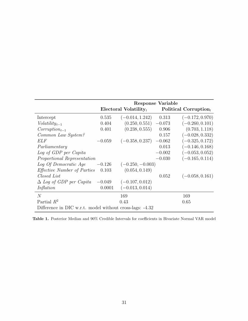
Response VariableElectoral Volatilityt Political Corruptiont

Intercept 0.535 (−0.014, 1.242) 0.313 (−0.172, 0.970)Volatility t−1 0.404 (0.250, 0.551) −0.073 (−0.260, 0.101)Corruptiont−1 0.401 (0.238, 0.555) 0.906 (0.703, 1.118)Common Law System? 0.157 (−0.028, 0.332)ELF −0.059 (−0.358, 0.237) −0.062 (−0.325, 0.172)Parliamentary 0.013 (−0.146, 0.168)Log of GDP per Capita −0.002 (−0.053, 0.052)Proportional Representation −0.030 (−0.165, 0.114)Log Of Democratic Age −0.126 (−0.250,−0.003)Effective Number of Parties 0.103 (0.054, 0.149)Closed List 0.052 (−0.058, 0.161)∆ Log of GDP per Capita −0.049 (−0.107, 0.012)Inflation 0.0001 (−0.013, 0.014)

N 169 169Partial R2 0.43 0.65Difference in DIC w.r.t. model without cross-lags: -4.32

Table 1. Posterior Median and 90% Credible Intervals for coefficients in Bivariate Normal VAR model

31

6 Figures and Tables

Vt-1

Ct-1 Ct

Vt...

...

...

...

Figure 1. Depiction of Granger Feedback Characterized Using VAR model parameters

32

Political Corruption at time t−1

Pre

dict

ed V

olat

ility

at t

ime

t

2.0 2.5 3.0 3.5 4.0 4.5

6.1

11.4

21.2

39.3

72.9

Figure 2. Predicted Values Of Volatility at time t As A Function of Lagged Corruption. Bars Represent90% Credible Intervals for the Predictions.

33

Electoral Volatility at time t−1

Pre

dict

ed C

orru

ptio

n at

tim

e t

1.8 2.7 7.4 20.1 54.6

2.5

3.0

3.5

4.0

Figure 3. Predicted Values Of Corruption at time t As A Function of Lagged Volatility. Bars Represent90% Credible Intervals for the Predictions.

34

Response VariableElectoral Volatilityt Political Corruptiont

Intercept −0.003 (−0.482, 0.513) 0.501 (0.204, 0.793)Volatility t−1 0.424 (0.312, 0.537) −0.141 (−0.368, 0.022)Corruptiont−1 0.466 (0.290, 0.613) 0.950 (0.811, 1.133)

N 169 169Partial R2 0.36 0.65Difference in DIC w.r.t. model without cross-lags: -41.98

Table 1. Posterior Median and 90% Credible Intervals for coefficients in Bivariate Normal VAR model

35

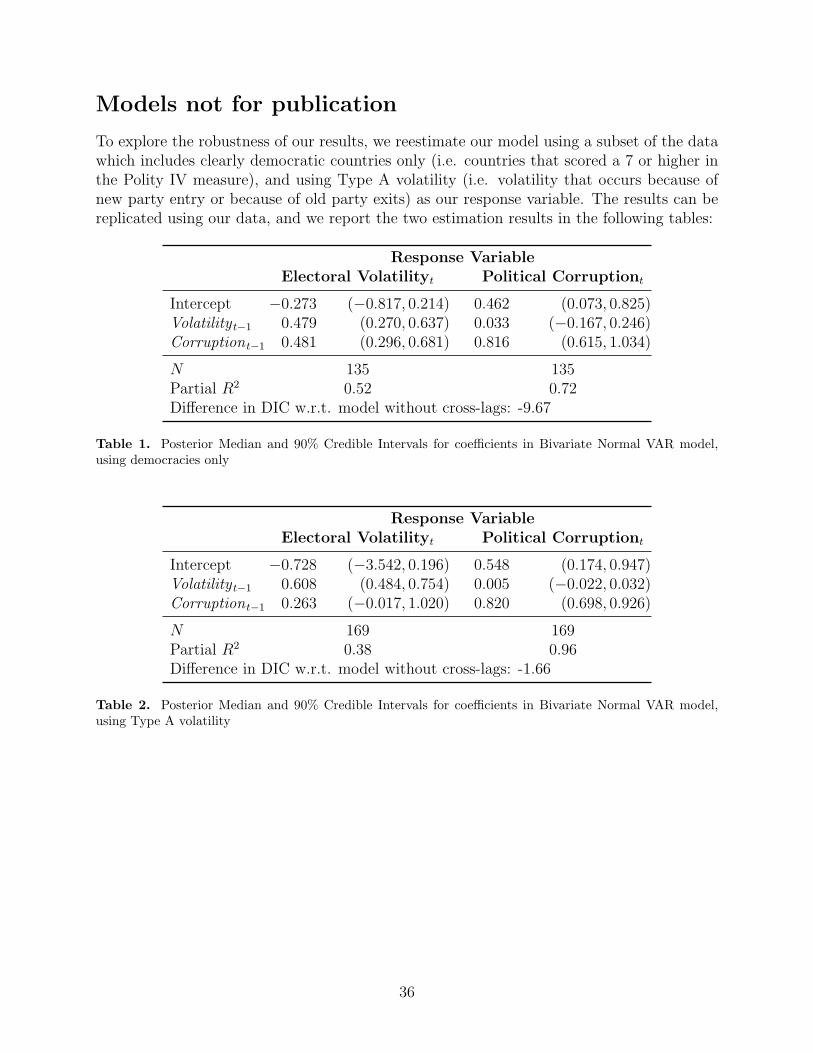
Models not for publication

To explore the robustness of our results, we reestimate our model using a subset of the datawhich includes clearly democratic countries only (i.e. countries that scored a 7 or higher inthe Polity IV measure), and using Type A volatility (i.e. volatility that occurs because ofnew party entry or because of old party exits) as our response variable. The results can bereplicated using our data, and we report the two estimation results in the following tables:

Response VariableElectoral Volatilityt Political Corruptiont

Intercept −0.273 (−0.817, 0.214) 0.462 (0.073, 0.825)Volatility t−1 0.479 (0.270, 0.637) 0.033 (−0.167, 0.246)Corruptiont−1 0.481 (0.296, 0.681) 0.816 (0.615, 1.034)

N 135 135Partial R2 0.52 0.72Difference in DIC w.r.t. model without cross-lags: -9.67

Table 1. Posterior Median and 90% Credible Intervals for coefficients in Bivariate Normal VAR model,using democracies only

Response VariableElectoral Volatilityt Political Corruptiont

Intercept −0.728 (−3.542, 0.196) 0.548 (0.174, 0.947)Volatility t−1 0.608 (0.484, 0.754) 0.005 (−0.022, 0.032)Corruptiont−1 0.263 (−0.017, 1.020) 0.820 (0.698, 0.926)

N 169 169Partial R2 0.38 0.96Difference in DIC w.r.t. model without cross-lags: -1.66

Table 2. Posterior Median and 90% Credible Intervals for coefficients in Bivariate Normal VAR model,using Type A volatility

36