CORRIDOR  DIAGNOSTIC  STUDY  OF  THE  NORTHERN  AND CENTRAL CORRIDORS OF EAST AFRICA 

ACTION PLAN   Volume 2: Technical Papers  B. Trade and Traffic Forecast  SUBMITTED TO    Task Coordination Group (TCG)  Chaired by East African Community (EAC) Alloys Mutabingwa  Deputy  Secretary  General  Planning  and Infrastructure Arusha, Tanzania   SUBMITTED BY     Nathan Associates Inc. Arlington, Virginia, USA  

April 15, 2011    

USAID Contract No. EEM‐I‐00‐07‐00009‐00, Order No. 2  with funding provided by USAID and DFID    

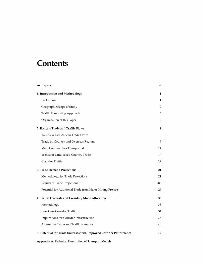
Contents  

Acronyms vi 

1. Introduction and Methodology 1 

Background 1 

Geographic Scope of Study 2 

Traffic Forecasting Approach 3 

Organization of this Paper 7 

2. Historic Trade and Traffic Flows 8 

Trends in East African Trade Flows 8 

Trade by Country and Overseas Regions 9 

Main Commodities Transported 14 

Trends in Landlocked Country Trade 17 

Corridor Traffic 17 

3. Trade Demand Projections 21 

Methodology for Trade Projections 21 

Results of Trade Projections 288 

Potential for Additional Trade from Major Mining Projects 29 

4. Traffic Forecasts and Corridor / Mode Allocation 33 

Methodology 33 

Base Case Corridor Traffic 34

Implications for Corridor Infrastructure 38

Alternative Trade and Traffic Scenarios 40

5. Potential for Trade Increases with Improved Corridor Performance 47 

Appendix A. Technical Description of Transport Models  

Illustrations

FIGURES

Figure 1-1. CDS Study Area 3

Figure 1-2. Traffic Forecasting Methodology 6

Figure 2-1. Distribution of East Africa Exports and Imports, 2008 8

Figure 2-2. Average Annual Growth of Imports and Exports by Country 2005-2009 10

Figure 2-3. Main Commodities Transported in the Northern Corridor, 2007 16

Figure 2-4 Main Commodities Transported in Central Corridor, 2010 16

Figure 2-5. Share of Transit Traffic by Corridor, 2009 20

Figure 3-1. Overview of Trade Forecast Methodology 24

Figure 3-2. Average Annual GDP Growth Used in the CDS Forecast, 2009-2030 26

Figure 3-3. Average Annual Trade Growth by Country, 2009-2015 and 2015-2030 30

Figure 4-1. Traffic Growth Forecast by Corridor 2009-2030 36

Figure 4-2. Base Case Corridor Traffic by Type, 2009-2030 37

Figure 4-3. Rail Share in Total Corridor Traffic by Type, 2009-2030 38

Figure 4-4. Comparison of Average Annual Trade Growth by Country, Base Case

vs. Low GDP Growth, 2009-2015 40

Figure 4-5. Comparison of Average Annual Trade Growth by Country Base Case

vs. Low GDP Growth, 2015-2030 41

Figure 4-6. Comparison of Traffic in Northern and Central Corridors Base Case

vs. Low GDP Growth Scenario, 2015 and 2030 43

Figure 4-7. Comparison of Traffic in Northern and Central Corridors: Base Case

vs. Worst Case Scenario, 2015 and 2030 45

TABLES

Table 2-1. Estimates of Import and Export Tonnages, 2008 11

Table 2-2. Estimates of Import and Export Tonnages in 2007 from NCIMP Study 12

Table 2-3. CDS Consolidated Estimates of Import and Export Tonnages in 2008 13

Table 2-4. Main Commodities Transported in the Northern Corridor, 2007 14

Table 2-5. Commodities Transported in the Central Corridor, 2010 15

Table 2-6. Trade Volumes of Landlocked Countries, 2005-2009 17

Table 2-7. Northern and Central Corridor Traffic by Type and Mode, 2009 18

Table 2-8. Transit Traffic by Country: Average Flows for 1999-2009 19

Table 2-9. Regional Trade by Corridor: Estimated Flows, 2009 20

Table 2-10 Forecast of Port Traffic by Type of Cargo, 2009-2030 21

Table 3-1. IMF Projected Annual GDP Growth, 2009-2015 23

Table 3-2. Projected Annual Average GDP Growth for CDS Countries 25

Table 3-3. Projected Annual Average GDP Growth for Overseas Regions 25

Table 3-4. Conversion Factors for Commodities Used to Obtain Tonnages 28

Table 3-6. East Africa Average Annual Growth Rates of Imports and Exports 29

Table 4-1. Base Case Traffic by Corridor and Mode, 2009 36

Table 4-2. Base Case Traffic by Corridor and Mode, 2015 36

Table 4-3. Base Case Traffic by Corridor and Mode, 2030 37

Table 4-4 Forecast of Port Traffic by Type of Cargo, 2009-2030 (000s tons) 39

Table 4-5. Low GDP Growth Traffic by Corridor and Mode, 2015 42

Table 4-6. Low GDP Growth Traffic by Corridor and Mode, 2030 42

Table 4-7. Worst Case Scenario Traffic by Corridor and Mode, 2015 44

Table 4-8. Worst Case Scenario Traffic by Corridor and Mode, 2030 45

Table 5-1. Potential for Traffic Increases due to Improved Corridor Performance, 2015 48

Table 5-2. Potential for Traffic Increases due to Improved Corridor Performance, 2030 48

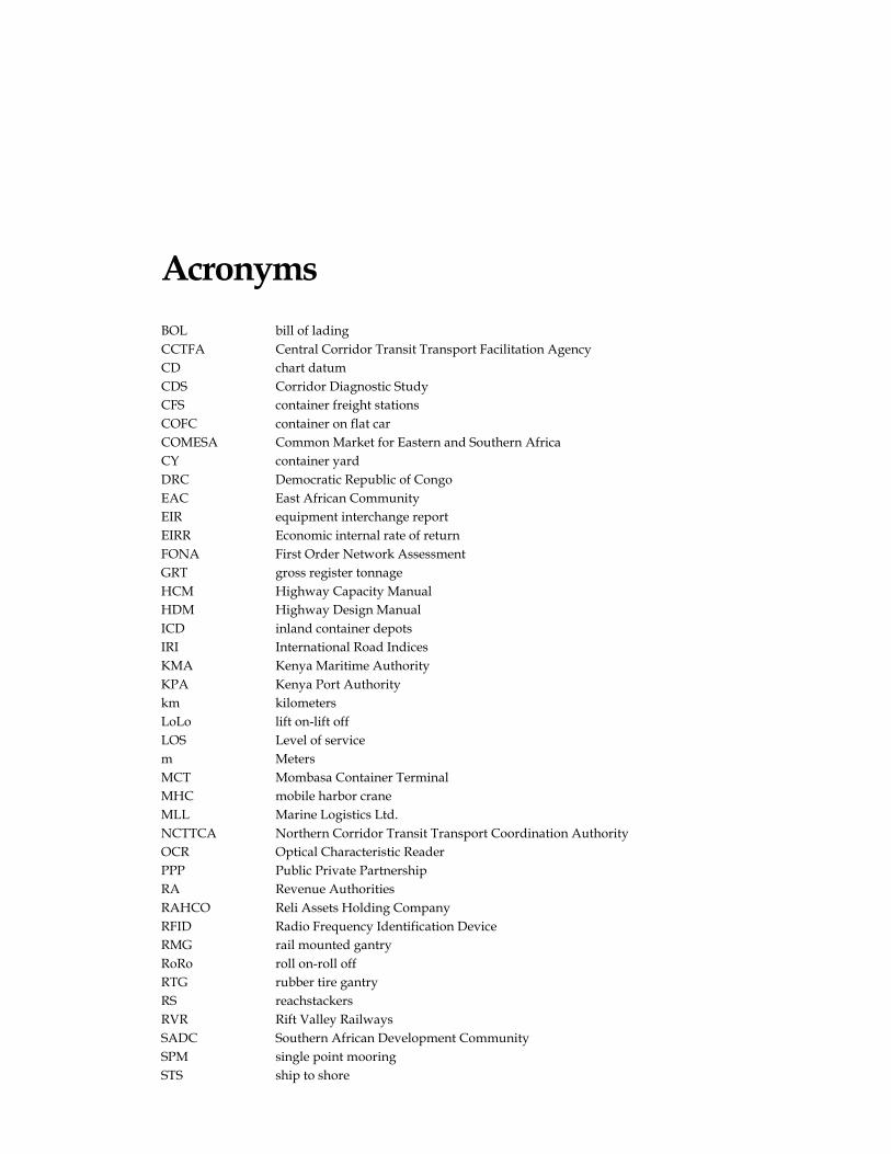
Acronyms BOL bill of lading CCTFA Central Corridor Transit Transport Facilitation Agency CD chart datum CDS Corridor Diagnostic Study CFS container freight stations COFC container on flat car COMESA Common Market for Eastern and Southern Africa CY container yard DRC Democratic Republic of Congo EAC East African Community EIR equipment interchange report EIRR Economic internal rate of return FONA First Order Network Assessment GRT gross register tonnage HCM Highway Capacity Manual HDM Highway Design Manual ICD inland container depots IRI International Road Indices KMA Kenya Maritime Authority KPA Kenya Port Authority km kilometers LoLo lift on-lift off LOS Level of service m Meters MCT Mombasa Container Terminal MHC mobile harbor crane MLL Marine Logistics Ltd. NCTTCA Northern Corridor Transit Transport Coordination Authority OCR Optical Characteristic Reader PPP Public Private Partnership RA Revenue Authorities RAHCO Reli Assets Holding Company RFID Radio Frequency Identification Device RMG rail mounted gantry RoRo roll on-roll off RTG rubber tire gantry RS reachstackers RVR Rift Valley Railways SADC Southern African Development Community SPM single point mooring STS ship to shore

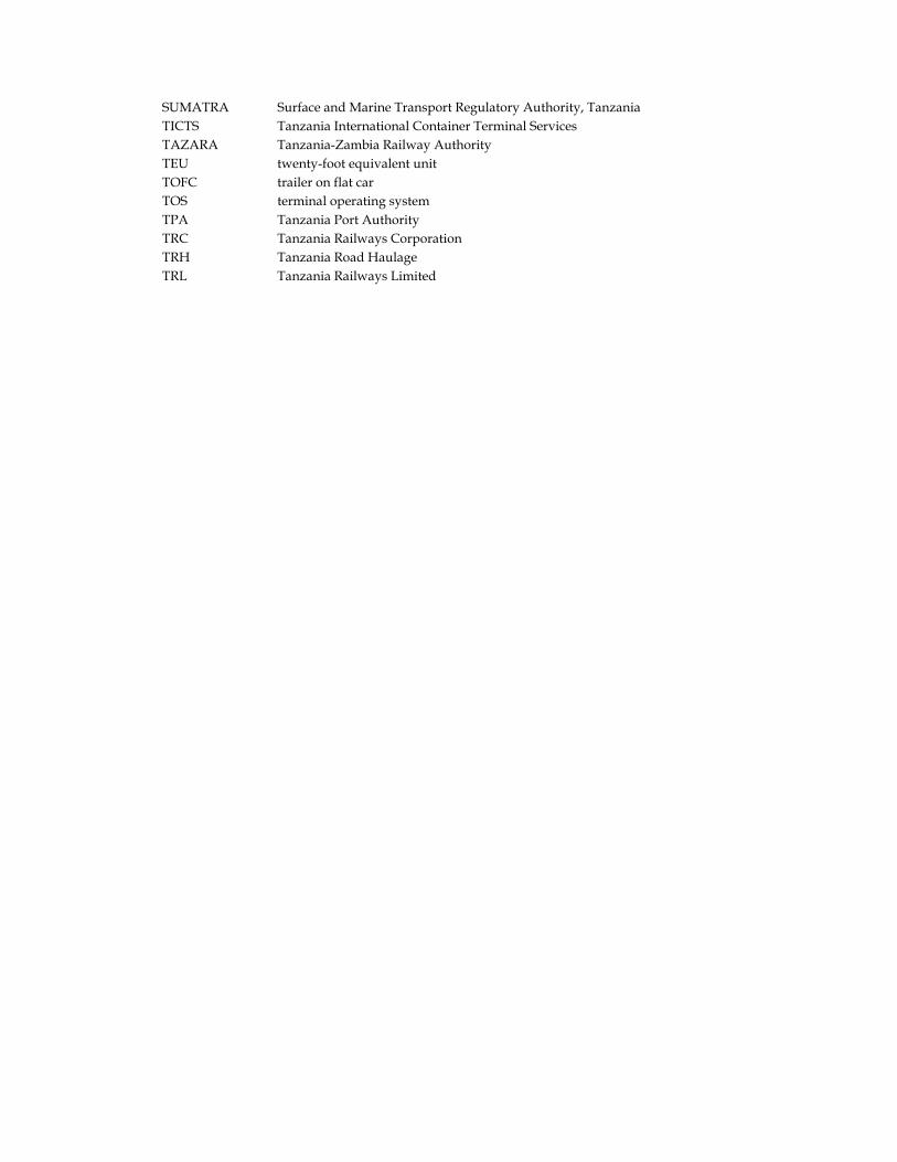
SUMATRA Surface and Marine Transport Regulatory Authority, Tanzania TICTS Tanzania International Container Terminal Services TAZARA Tanzania-Zambia Railway Authority TEU twenty-foot equivalent unit TOFC trailer on flat car TOS terminal operating system TPA Tanzania Port Authority TRC Tanzania Railways Corporation TRH Tanzania Road Haulage TRL Tanzania Railways Limited

1. Introduction and Methodology

Background

The Northern Corridor anchored by the port of Mombasa in Kenya, and the Central Corridor, anchored by the port of Dar es Salaam in Tanzania, are principal and crucial transport routes for national, regional and

international trade of the five East African Community (EAC) countries, namely; Burundi, Kenya, Rwanda,

Tanzania and Uganda. Due to inadequate physical infrastructure and inefficiency, these corridors are characterized by long transit times and high cost. Freight costs per km are more than 50 percent higher

than the USA and Europe and for the landlocked countries; transport costs can be as high as 75 percent of

the value of exports. Modernization of transport infrastructure and removal of non-tariff barriers along these corridors is critical for trade expansion and economic growth, which are key to the success of regional

integration as well as creation of wealth and poverty alleviation in the individual countries.

The Heads of State in the COMESA, EAC and SADC, the Tripartite, have determined that the transport inefficiencies are among the biggest impediments to realizing their vision to lead their countries out of

poverty. Transport costs are prohibitively high and are a barrier to trade and investment, which are the

cornerstone for the aspired economic growth to regional prosperity.

Having had the experience of successful development of an action plan to effectively tackle transport

bottlenecks on the North-South Corridor, the Tripartite have ordered the preparation of a similar action

plan for the key trade routes of Eastern Africa. As a technical foundation for the action plan, regional stakeholders in March 2009 agreed to carry out a Corridor Diagnostic Study (CDS) with funding from the

U.S. Agency for International Development (USAID) and the U.K. Department for International

Development (DFID).

This Technical Paper presents the CDS forecast of trade and traffic for the Northern and Central Corridors.

An overview of historical trade and traffic patterns in the Northern and Central Corridors, including

discussions of types of traffic, modes utilized and commodities transported is provided. The traffic forecast methodology is described; involving models for trade demand forecasts, corridor and mode allocation and

the impact of improved corridor performance parameters on future trade. The emphasis of this paper is on

the estimation of the impact of improved performance resulting from proposed projects on the allocation of traffic to corridors and modes; while estimating impact on trade takes a secondary role. The technical paper

summarizes selected results of traffic analysis and surveys carried out by Nathan Associates for the

Northern and Central Corridors of East Africa. This paper also utilizes the results reported in two

2

separate ongoing studies: The Northern Corridor Infrastructure Master Plan (NCIMP) being implemented

by Louis Berger for the Northern Corridor Transit Coordination Authority1 and the Definition and Investment Strategy for a Core Strategic Transport Network for Eastern and Southern Africa (Core

Network Study) being implemented by Nathan Associates, Inc. for the World Bank.2 The results of these

two studies were used as part of the input to the analysis and forecasts in this working paper. Other

sources were also included as described in the methodology below.

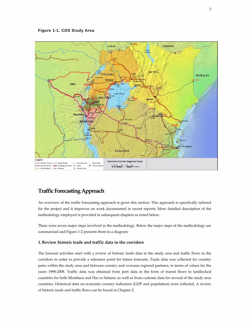
Geographic Scope of Study

The Corridor Diagnostic Study reviewed the infrastructure condition and regulatory policy of the Northern

Corridor anchored by the port of Mombasa in Kenya, and the Central Corridor, anchored by the port of

Dar es Salaam in Tanzania, which are principal and crucial transport routes for national, regional and international trade of the five East African Community (EAC) countries, namely; Burundi, Kenya, Rwanda,

Tanzania and Uganda (see Figure 1-1). The CDS analysis also includes the extension of the Northern and

Central Corridors to the Democratic Republic of the Congo and links to Southern Sudan, Ethiopia and

Zambia.

1 Northern Corridor Infrastructure Master Plan: Interim Report: Interim Report, June 2010. 2 Definition and Investment Strategy for a Core Strategic Transport Network for Eastern and Southern Africa, Regional Model

Report, June 2010.

3

Figure 1-1. CDS Study Area

Traffic Forecasting Approach

An overview of the traffic forecasting approach is given this section. This approach is specifically tailored

for the project and it improves on work documented in recent reports: More detailed description of the methodology employed is provided in subsequent chapters as noted below.

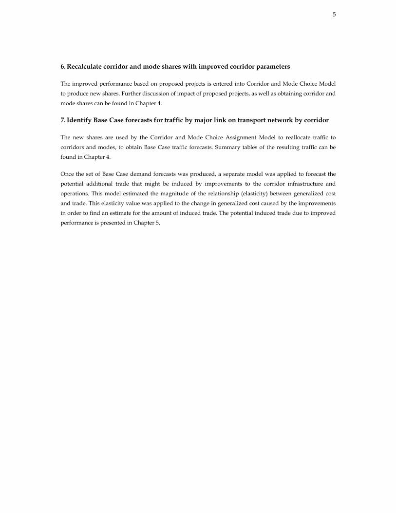
There were seven major steps involved in the methodology. Below the major steps of the methodology are

summarized and Figure 1-2 presents them in a diagram:

1. Review historic trade and traffic data in the corridors

The forecast activities start with a review of historic trade data in the study area and traffic flows in the

corridors in order to provide a reference point for future forecasts. Trade data was collected for country

pairs within the study area and between country and overseas regional partners, in terms of values for the

years 1998-2008. Traffic data was obtained from port data in the form of transit flows to landlocked

countries for both Mombasa and Dar es Salaam; as well as from customs data for several of the study area countries. Historical data on economic country indicators (GDP and population) were collected. A review

of historic trade and traffic flows can be found in Chapter 2.

4

2. Produce GDP and population forecasts

Data on GDP and population values for CDS study area countries were collected, reviewed and cleaned. Once reorganized, the historical economic data was used to forecast future values from 2009 to 2030. The

results were compared and contrasted with the country economic forecasts in the reference studies;

adjustments were made where necessary to render the data more accurate.

3. Create forecast of trade flows

First, using the data collected on historical trade flows, GDP and population in the first step and the

forecasts calculated in the second step, total trade values for all countries in the study area were estimated.

Then, trade values (import and export flows) for trading partners were forecasted from 2009 to 2030,

through a regression model. Trade shares obtained from the results of the regression model were applied

to total regional trade obtained from country level trade values, and produced the trade forecasts. The adjusted results in values were finally converted into tonnages; through conversion factors using

commodities the study area countries trade. A detailed explanation of this methodology and summary

tables of the results of trade forecasts can be found in Chapter 3.

4. Assign trade flows to corridors and modes to obtain status quo traffic forecasts

Once demand was estimated between trading partners, trade flows were assigned to corridors, by mode:

road, rail and ports. The allocation was based on corridor performance data (price, time and reliability as perceived by shippers) estimated by FastPath, socioeconomic indicators (language groupings and

economic association groupings), and policy indicators (mode preference for certain types of traffic and

preference for or bias against specific ports or countries)3. This activity produces a set of status quo traffic

forecasts, meaning that the forecasts assume that only regular upgrade, maintenance and expansion works

of the corridor are incorporated; excluding any proposed projects that would lead to improvements in

corridor performance. This analysis was done for years 2015 and 2030.

5. Identify potential impact of proposed projects on corridor performance

In order to estimate the impact of the proposed projects, their localized impact on performance variables

(time, cost, reliability) was coded into FastPath for each link, node or logistics component. From FastPath, we obtained corridor level performance results, which were then compared against status quo baseline to

estimate impact.

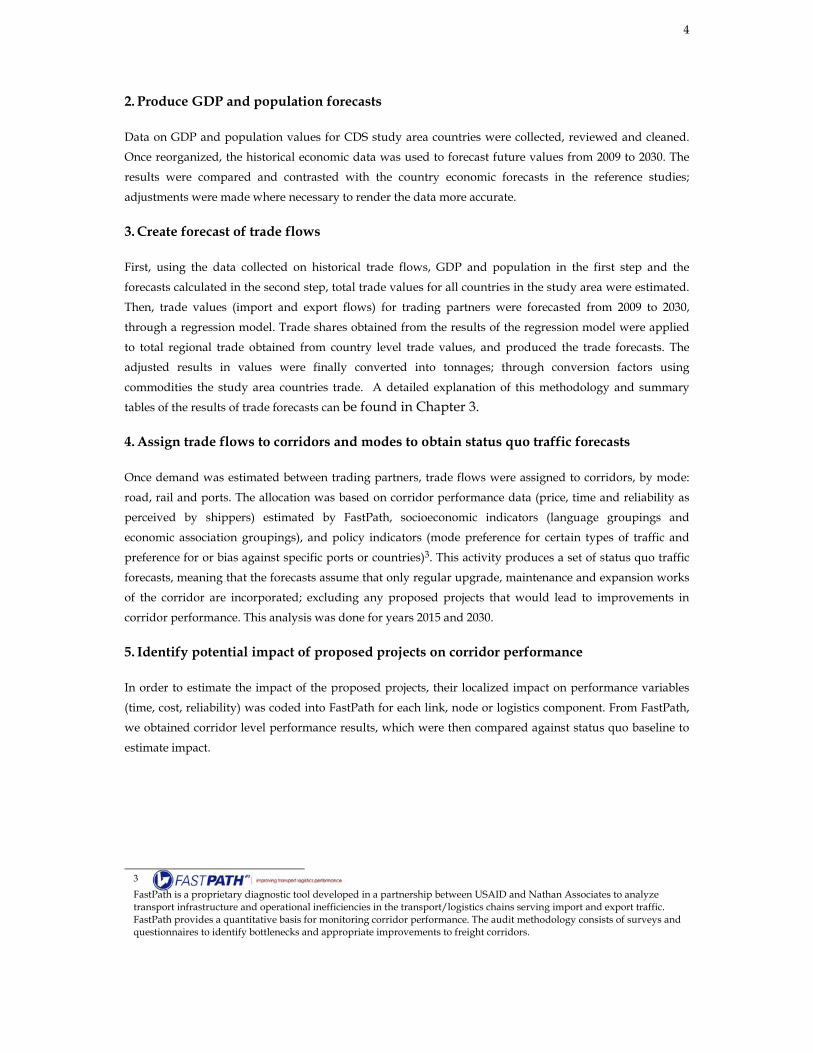
3 FastPath is a proprietary diagnostic tool developed in a partnership between USAID and Nathan Associates to analyze transport infrastructure and operational inefficiencies in the transport/logistics chains serving import and export traffic. FastPath provides a quantitative basis for monitoring corridor performance. The audit methodology consists of surveys and questionnaires to identify bottlenecks and appropriate improvements to freight corridors.

5

6. Recalculate corridor and mode shares with improved corridor parameters

The improved performance based on proposed projects is entered into Corridor and Mode Choice Model

to produce new shares. Further discussion of impact of proposed projects, as well as obtaining corridor and

mode shares can be found in Chapter 4.

7. Identify Base Case forecasts for traffic by major link on transport network by corridor

The new shares are used by the Corridor and Mode Choice Assignment Model to reallocate traffic to

corridors and modes, to obtain Base Case traffic forecasts. Summary tables of the resulting traffic can be found in Chapter 4.

Once the set of Base Case demand forecasts was produced, a separate model was applied to forecast the

potential additional trade that might be induced by improvements to the corridor infrastructure and

operations. This model estimated the magnitude of the relationship (elasticity) between generalized cost

and trade. This elasticity value was applied to the change in generalized cost caused by the improvements

in order to find an estimate for the amount of induced trade. The potential induced trade due to improved performance is presented in Chapter 5.

6

Figure 1-2. Traffic Forecasting Methodology

4

5

2. Produce GDP and

population forecasts

Review country economic forecasts in the Northern Corridor Infrastructure Master

Plan

Review country economic forecasts in

the Core Network Study

3. Create forecast of trade flows

1. Review historic trade and traffic data in the corridors

Review transport demand and traffic forecasts Northern

Corridor Infrastructure Master Plan

Review international trade demand

forecasts from the Core Network Study

4. Assign trade flows to corridors and modes to obtain

status quo traffic forecasts

5. Identify potential impact of proposed

projects on corridor performance Apply model of trade

relationships to corridor performance

7. Identify Base Case forecasts for traffic by major

link on transport network by corridor

Identify potential increases in trade

flows due to corridor improvements

6. Recalculate corridor and mode

shares with improved corridor

parameters

7

Organization of this Paper

Following this introductory chapter, Chapter 2 presents the historic trade and traffic flows in the two

corridors. Chapter 3 presents the trade demand projections by country for 2015 and 2030. Chapter 4 shows

how trade is assigned to corridors and modes; then presents forecasts for status quo and Base Case scenarios. Chapter 5 identifies and quantifies how potential improvements in corridor performance affect

forecasted traffic.

8

2. Historic Trade and Traffic Flows This section discusses orientation of East African trade; presents the collected data on East Africa’s historic

trade between trading partners, which were used as a basis for trade and traffic forecasts; identifies main commodities transported in corridors; presents historical corridor traffic, including past growth of overseas

trade with landlocked countries and discusses implications of these trends for corridor infrastructure.

Trends in East African Trade Flows

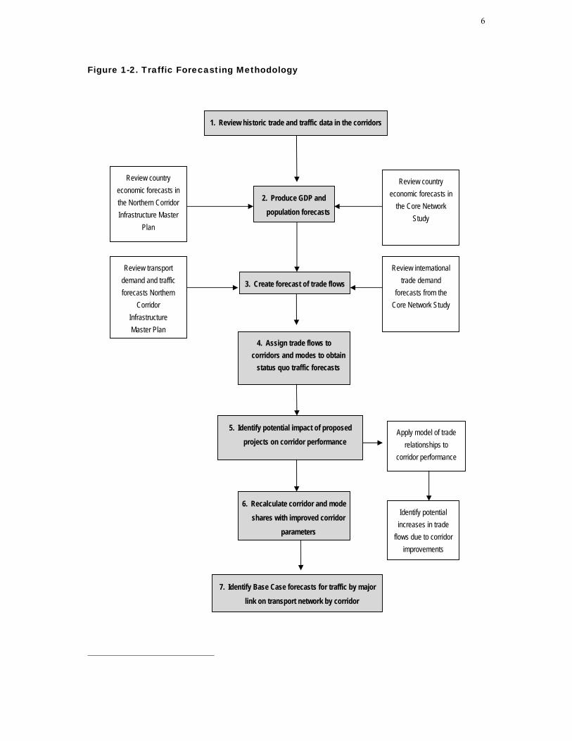
As in other parts of Africa, East African trade is very overseas-oriented. Total East African trade was 34.5

million tons in 2008, consisting of 27 million of imports ( 78.4 percent) and 7.5 million of exports (21.6

percent). Most of its exports and imports are with overseas partners (62 and 78 percent respectively), while

the rest stay within East Africa region (30 and 8 percent) and with other African countries (8 and 14

percent). This is shown graphically in Figure 2-16.

Figure 2-1. Distribution of East Africa Exports and Imports, 2008

Source: : IMF Direction of Trade Statistics and COMTRADE.

6 The “Study Area” is defined as the following eight countries: Burundi, Congo DR (Eastern), Ethiopia, Kenya, Rwanda, Sudan

(Southern), Tanzania, Uganda , while “Other Africa”is defined as the countries in the African continent other than East Africa region.

9

Trade by Country and Overseas Regions

Initially, trade values (in million USD) were obtained from IMF Direction of Trade Statistics for the years covering 1998-2008. As a first step, historical trade flows with Africa region and with overseas partners

were reviewed. Some observations on common characteristics and trends are below:

• Countries with a recent history of conflict and economic crises had very low or negative trade growth in the last decade. The most prominent examples are DR Congo with high negative trade growth

rates and Burundi with low import growth rates. Countries that had conflict earlier had high growth

rates reflecting recovery, such as Rwanda.

• Export growth rates tend to be faster for overseas trade than those for imports.

• Overseas trade is higher in unit value than trade within Africa. We see a generally increasing trend in

overseas trade.

• Europe used to be a major trading partner but its share in total trade seems to be gradually

decreasing for most East African countries.

• East Asia is an emerging trading partner for East Africa and its imports from East Africa are projected to increase continuously.

• In the recent past, there are certain countries with high short term growth rates (e.g., 34 percent

import growth to overseas regions for DR Congo). However, the growth rates for these countries are expected to stabilize at lower levels in the long run.

As a second step, trade values were converted into tonnages, using factors estimated per commodity group

and port tonnage data for overseas trade. The country’s mix of commodities was taken into consideration

for the conversions. Estimates of trade tonnage values by country and overseas regions are presented in

Table 2-1.

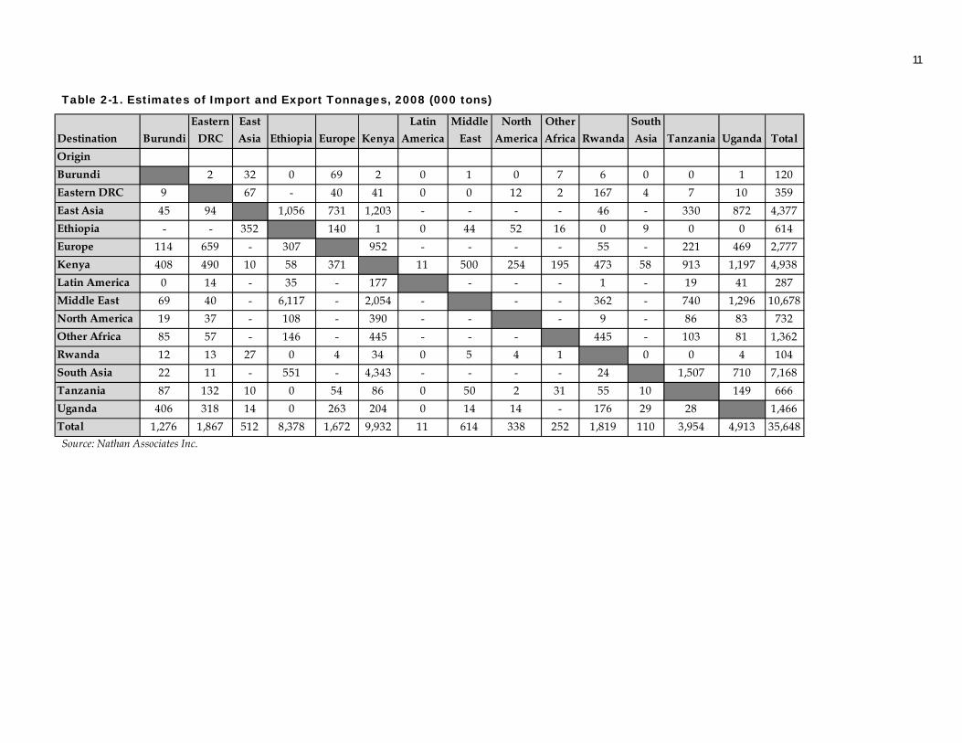
The estimates of trade tonnage by country and overseas regions in the Corridor Diagnostic Study are presented in Table 2-1. The estimates are based on conversions of trade values from IMF Direction of Trade

Statistics using factors by commodity group, supplemented by port tonnage data in the case of overseas

trade. The data includes trade with major overseas partners, which were derived from trade value data adjusted for the mix of commodities. However, it excludes trade with Southern Sudan and the Ethiopia

trade with Kenya is shown for all trade including trade which uses the Port of Djibouti.

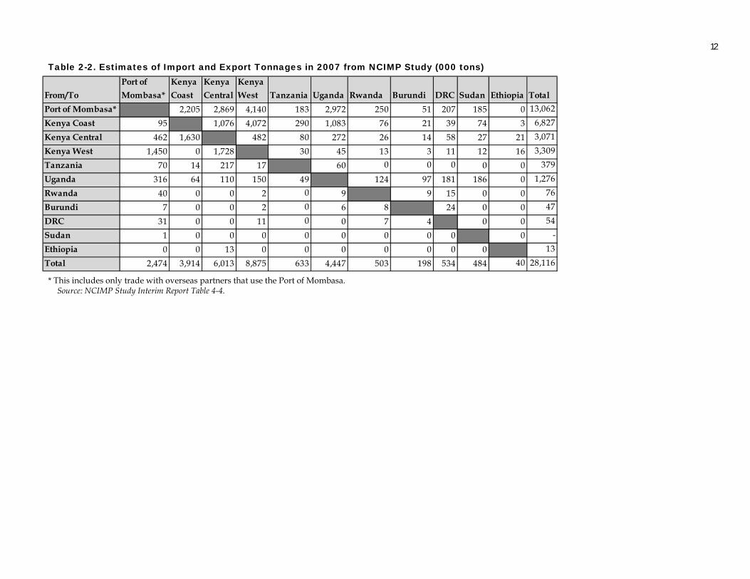
Table 2-2 presents similar data from the NCIMP report, which was derived from an analysis of trade tonnage volumes. This involved reconciling the international trade statistics in tonnages using a surplus-

deficit analysis technique. This table gives more detail on the origins and destinations of this trade within

Kenya (three regions) but it only includes trade with overseas partners that passed through the Port of

Mombasa (i.e., no overseas trade that used the Central Corridor). Ethiopian trade is shown only for Kenya,

since that is the trade that uses the Port of Mombasa and/or the Northern Corridor. This is the main

difference between the total volumes in Tables 2-1 and 2-2.

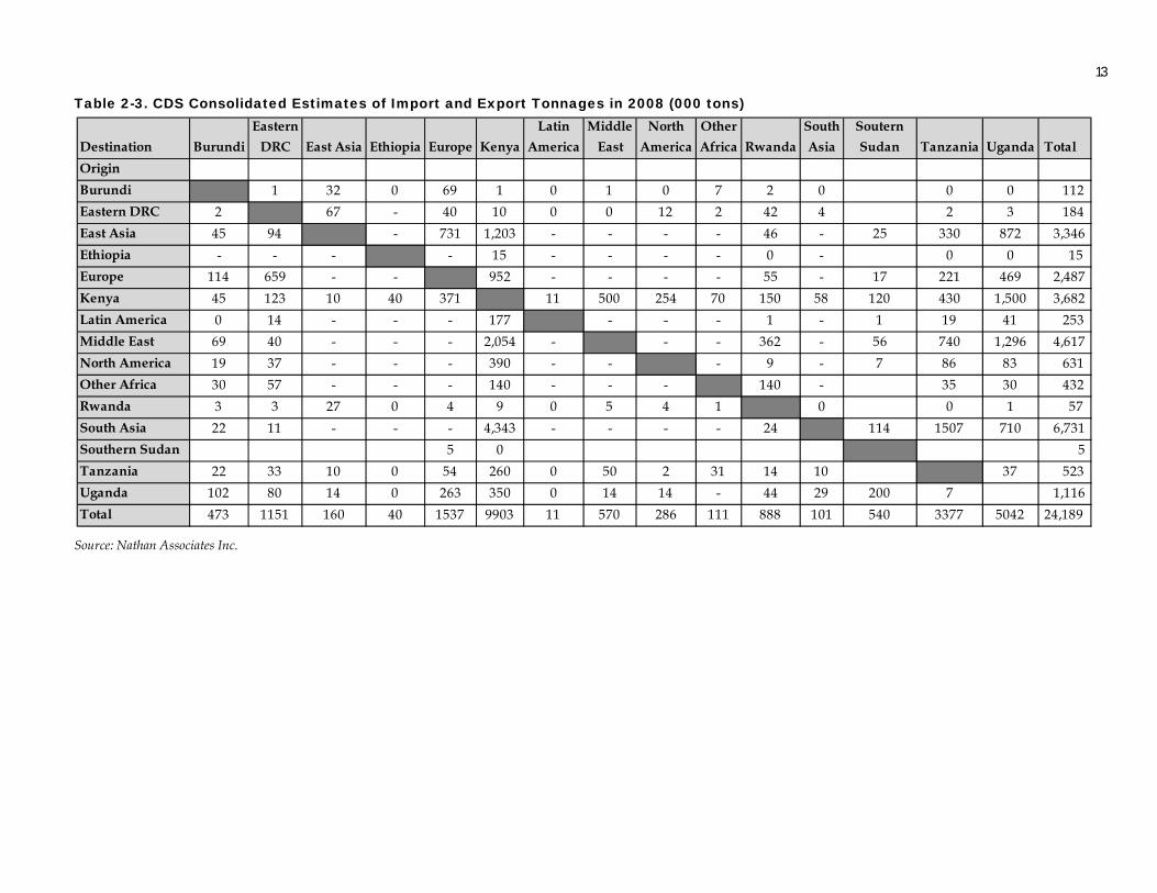
Table 2-3 consolidates the two data sets, showing the detail of trade with overseas partners for both

Northern and Central Corridors and trade for Southern Sudan but limiting Ethiopian data to trade with

10

Kenya and Tanzania. The Sudan data also includes trade between Kenya and Northern Sudan which

comes through the Port of Mombasa (primarily Kenyan exports to the Sudan). The 2007 data consolidated from the NCIMP table was increased slightly to arrive at 2008 values. The overall change is that exports to

overseas partners increased by 6 million tons over the NCIMP figures for the Port of Mombasa to account

for flows through Dar es Salaam port, and imports increased by about 300,000 tons over the NCIMP figures

for the same reason.

The consolidated data table was created in by adding data from Ethiopia and Sudan to the CDS data set

and adjusting all data to match port traffic statistics for transit traffic by country in the base year. The total tonnage in the consolidated table (24.2 million tons) is less than the total NCIMP figure of 28.1 million tons

due to the subtraction of internal trade between regions in Kenya from the consolidated total, which

represents only imports and exports.

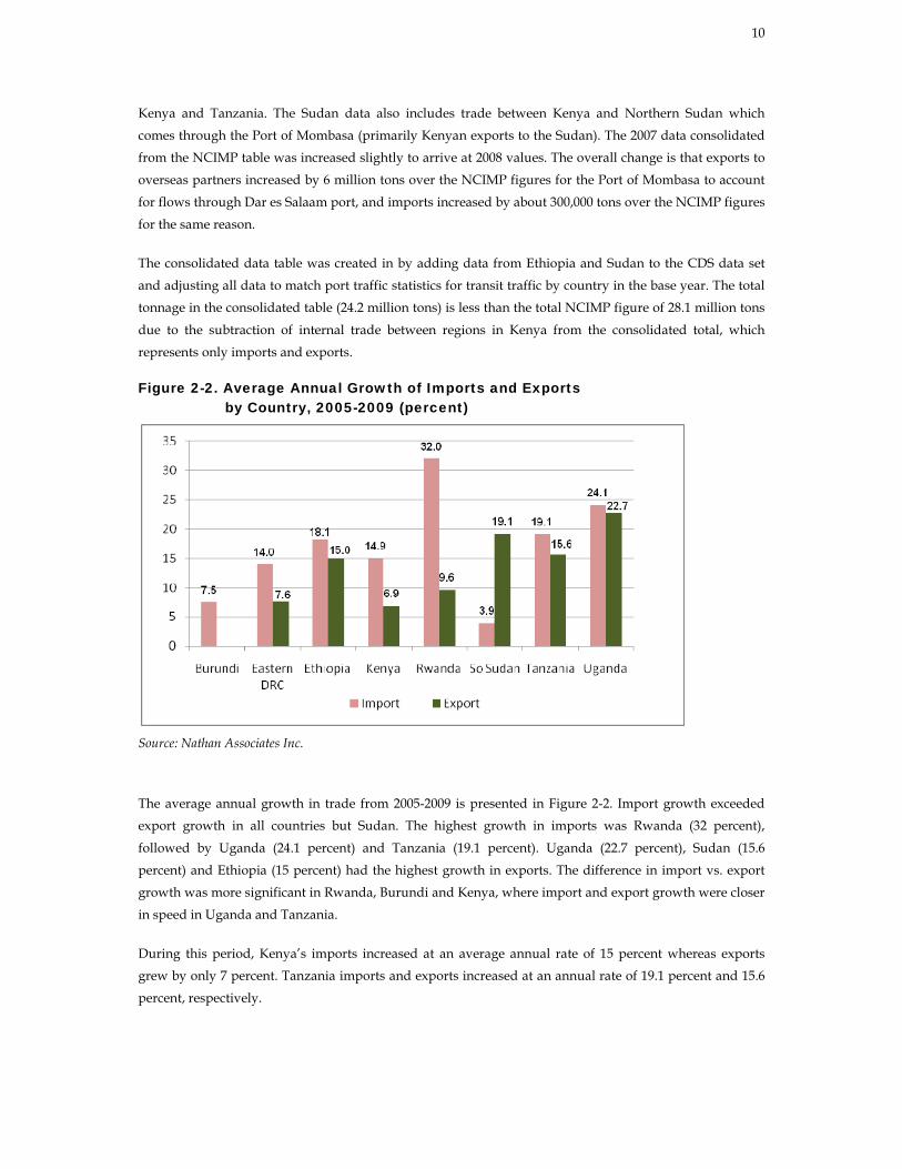
Figure 2-2. Average Annual Growth of Imports and Exports by Country, 2005-2009 (percent)

Source: Nathan Associates Inc.

The average annual growth in trade from 2005-2009 is presented in Figure 2-2. Import growth exceeded export growth in all countries but Sudan. The highest growth in imports was Rwanda (32 percent),

followed by Uganda (24.1 percent) and Tanzania (19.1 percent). Uganda (22.7 percent), Sudan (15.6

percent) and Ethiopia (15 percent) had the highest growth in exports. The difference in import vs. export growth was more significant in Rwanda, Burundi and Kenya, where import and export growth were closer

in speed in Uganda and Tanzania.

During this period, Kenya’s imports increased at an average annual rate of 15 percent whereas exports grew by only 7 percent. Tanzania imports and exports increased at an annual rate of 19.1 percent and 15.6

percent, respectively.

11

Destination BurundiEastern

DRCEast Asia Ethiopia Europe Kenya

Latin America

Middle East

North America

Other Africa Rwanda

South Asia Tanzania Uganda Total

OriginBurundi 2 32 0 69 2 0 1 0 7 6 0 0 1 120Eastern DRC 9 67 - 40 41 0 0 12 2 167 4 7 10 359East Asia 45 94 1,056 731 1,203 - - - - 46 - 330 872 4,377Ethiopia - - 352 140 1 0 44 52 16 0 9 0 0 614Europe 114 659 - 307 952 - - - - 55 - 221 469 2,777Kenya 408 490 10 58 371 11 500 254 195 473 58 913 1,197 4,938Latin America 0 14 - 35 - 177 - - - 1 - 19 41 287Middle East 69 40 - 6,117 - 2,054 - - - 362 - 740 1,296 10,678North America 19 37 - 108 - 390 - - - 9 - 86 83 732Other Africa 85 57 - 146 - 445 - - - 445 - 103 81 1,362Rwanda 12 13 27 0 4 34 0 5 4 1 0 0 4 104South Asia 22 11 - 551 - 4,343 - - - - 24 1,507 710 7,168Tanzania 87 132 10 0 54 86 0 50 2 31 55 10 149 666Uganda 406 318 14 0 263 204 0 14 14 - 176 29 28 1,466Total 1,276 1,867 512 8,378 1,672 9,932 11 614 338 252 1,819 110 3,954 4,913 35,648

Table 2-1. Estimates of Import and Export Tonnages, 2008 (000 tons)

Source: Nathan Associates Inc.

12

From/ToPort of Mombasa*

Kenya Coast

Kenya Central

Kenya West Tanzania Uganda Rwanda Burundi DRC Sudan Ethiopia Total

Port of Mombasa* 2,205 2,869 4,140 183 2,972 250 51 207 185 0 13,062Kenya Coast 95 1,076 4,072 290 1,083 76 21 39 74 3 6,827Kenya Central 462 1,630 482 80 272 26 14 58 27 21 3,071Kenya West 1,450 0 1,728 30 45 13 3 11 12 16 3,309Tanzania 70 14 217 17 60 0 0 0 0 0 379Uganda 316 64 110 150 49 124 97 181 186 0 1,276Rwanda 40 0 0 2 0 9 9 15 0 0 76Burundi 7 0 0 2 0 6 8 24 0 0 47DRC 31 0 0 11 0 0 7 4 0 0 54Sudan 1 0 0 0 0 0 0 0 0 0 -Ethiopia 0 0 13 0 0 0 0 0 0 0 13Total 2,474 3,914 6,013 8,875 633 4,447 503 198 534 484 40 28,116

Table 2-2. Estimates of Import and Export Tonnages in 2007 from NCIMP Study (000 tons)

* This includes only trade with overseas partners that use the Port of Mombasa. Source: NCIMP Study Interim Report Table 4-4.

13

Destination BurundiEastern

DRC East Asia Ethiopia Europe KenyaLatin

AmericaMiddle

EastNorth

AmericaOther Africa Rwanda

South Asia

Soutern Sudan Tanzania Uganda Total

OriginBurundi 1 32 0 69 1 0 1 0 7 2 0 0 0 112 Eastern DRC 2 67 - 40 10 0 0 12 2 42 4 2 3 184 East Asia 45 94 - 731 1,203 - - - - 46 - 25 330 872 3,346 Ethiopia - - - - 15 - - - - 0 - 0 0 15 Europe 114 659 - - 952 - - - - 55 - 17 221 469 2,487 Kenya 45 123 10 40 371 11 500 254 70 150 58 120 430 1,500 3,682 Latin America 0 14 - - - 177 - - - 1 - 1 19 41 253 Middle East 69 40 - - - 2,054 - - - 362 - 56 740 1,296 4,617 North America 19 37 - - - 390 - - - 9 - 7 86 83 631 Other Africa 30 57 - - - 140 - - - 140 - 35 30 432 Rwanda 3 3 27 0 4 9 0 5 4 1 0 0 1 57 South Asia 22 11 - - - 4,343 - - - - 24 114 1507 710 6,731 Southern Sudan 5 0 5 Tanzania 22 33 10 0 54 260 0 50 2 31 14 10 37 523 Uganda 102 80 14 0 263 350 0 14 14 - 44 29 200 7 1,116 Total 473 1151 160 40 1537 9903 11 570 286 111 888 101 540 3377 5042 24,189

Table 2-3. CDS Consolidated Estimates of Import and Export Tonnages in 2008 (000 tons)

Source: Nathan Associates Inc.

Volume (000s tons)

Oil 4,973 26Grains and flours 1,894 10Clinker and stones 1,338 7Vegetable oils 951 5Cast iron, Iron and Steel 787 4Sugar 532 3Fertilizer 429 2Cement 719 4Tea 465 2Soda 387 2Vegetables 310 2Coffee 263 1Various ores 26 0Total Selection 13,074 68

Commodity Type Commodity Share in Total Trade (%)

Commodities Mainly Imported

Mainly local production

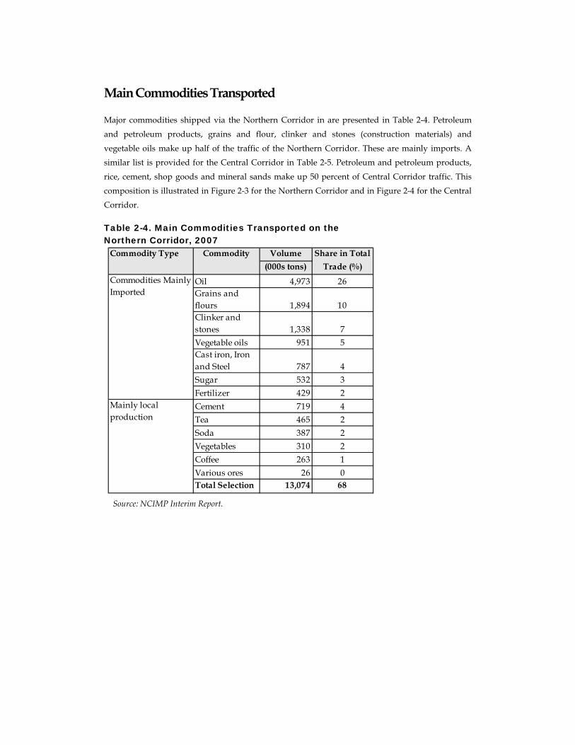
Main Commodities Transported

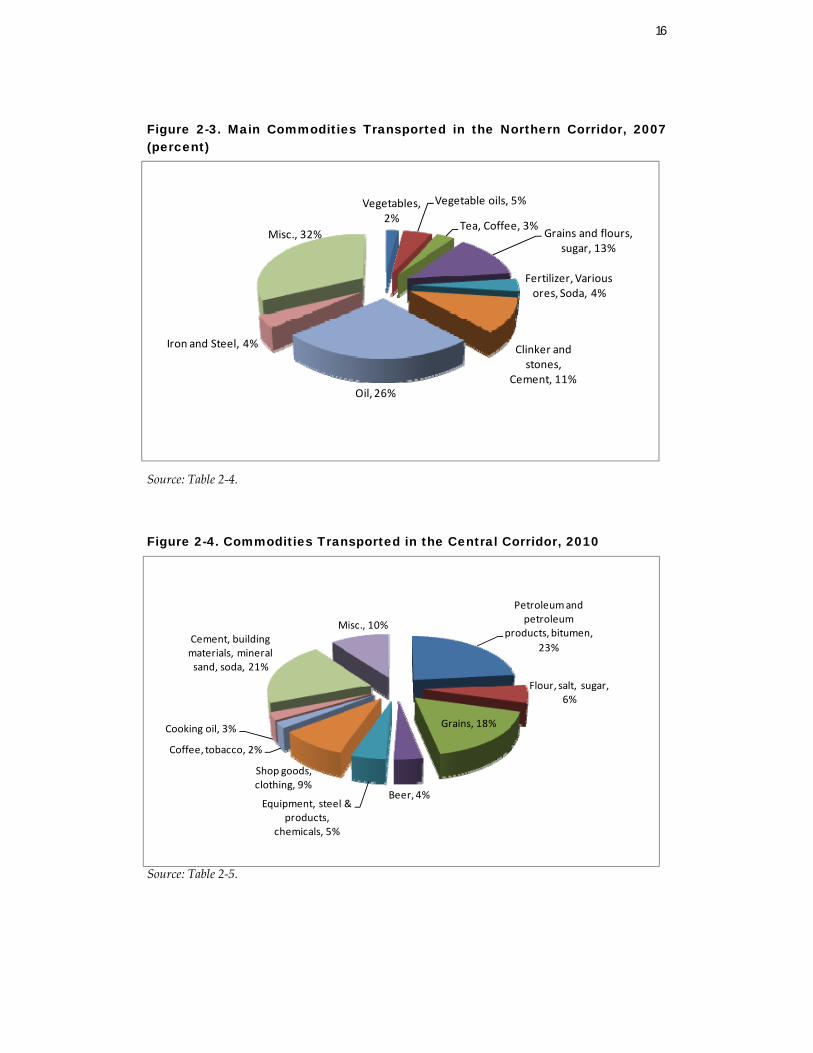
Major commodities shipped via the Northern Corridor in are presented in Table 2-4. Petroleum

and petroleum products, grains and flour, clinker and stones (construction materials) and

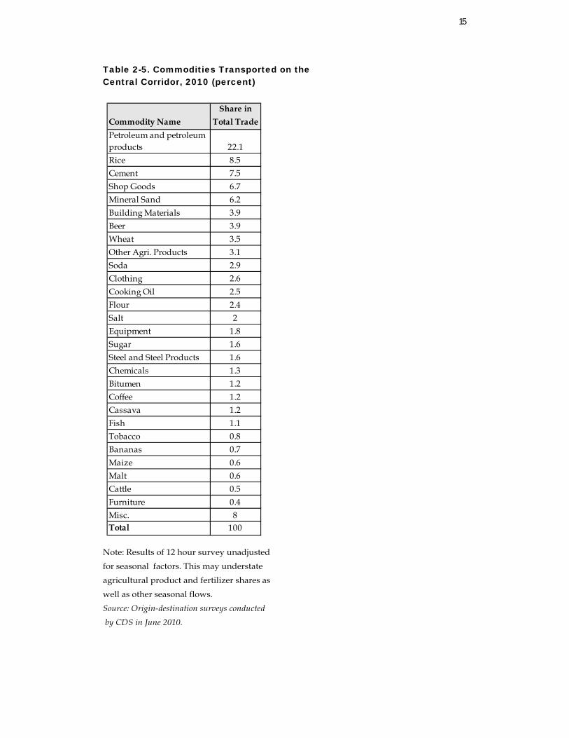
vegetable oils make up half of the traffic of the Northern Corridor. These are mainly imports. A similar list is provided for the Central Corridor in Table 2-5. Petroleum and petroleum products,

rice, cement, shop goods and mineral sands make up 50 percent of Central Corridor traffic. This

composition is illustrated in Figure 2-3 for the Northern Corridor and in Figure 2-4 for the Central Corridor.

Table 2-4. Main Commodities Transported on the Northern Corridor, 2007

Source: NCIMP Interim Report.

15

Commodity NameShare in

Total TradePetroleum and petroleum products 22.1Rice 8.5Cement 7.5Shop Goods 6.7Mineral Sand 6.2Building Materials 3.9Beer 3.9Wheat 3.5Other Agri. Products 3.1Soda 2.9Clothing 2.6Cooking Oil 2.5Flour 2.4Salt 2Equipment 1.8Sugar 1.6Steel and Steel Products 1.6Chemicals 1.3Bitumen 1.2Coffee 1.2Cassava 1.2Fish 1.1Tobacco 0.8Bananas 0.7Maize 0.6Malt 0.6Cattle 0.5Furniture 0.4Misc. 8Total 100

Table 2-5. Commodities Transported on the Central Corridor, 2010 (percent)

 

Note: Results of 12 hour survey unadjusted for seasonal factors. This may understate

agricultural product and fertilizer shares as

well as other seasonal flows.

Source: Origin-destination surveys conducted

by CDS in June 2010.

16

Vegetables, 2%

Vegetable oils, 5%

Tea, Coffee, 3%Grains and flours, 

sugar, 13%

Fertilizer, Various ores, Soda, 4%

Clinker and stones, 

Cement, 11%Oil, 26%

Iron and Steel, 4%

Misc., 32%

Petroleum and petroleum 

products, bitumen, 23%

Flour, salt,  sugar, 6%

Grains, 18%

Beer, 4%Equipment, steel & 

products, chemicals, 5%

Shop goods, clothing, 9%

Coffee, tobacco, 2%

Cooking oil, 3%

Cement, building materials, mineral sand, soda, 21%

Misc., 10%

Figure 2-3. Main Commodities Transported in the Northern Corridor, 2007 (percent)

Source: Table 2-4.

Figure 2-4. Commodities Transported in the Central Corridor, 2010

Source: Table 2-5.

17

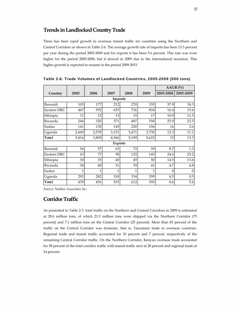
Trends in Landlocked Country Trade

There has been rapid growth in overseas transit traffic for countries using the Northern and

Central Corridors as shown in Table 2-6. The average growth rate of imports has been 13.3 percent

per year during the period 2005-2009 and for exports it has been 5.6 percent. This rate was even higher for the period 2005-2008, but it slowed in 2009 due to the international recession. This

higher growth is expected to resume in the period 2009-2015.

Table 2-6. Trade Volumes of Landlocked Countries, 2005-2009 (000 tons)

Source: Nathan Associates Inc.

Corridor Traffic

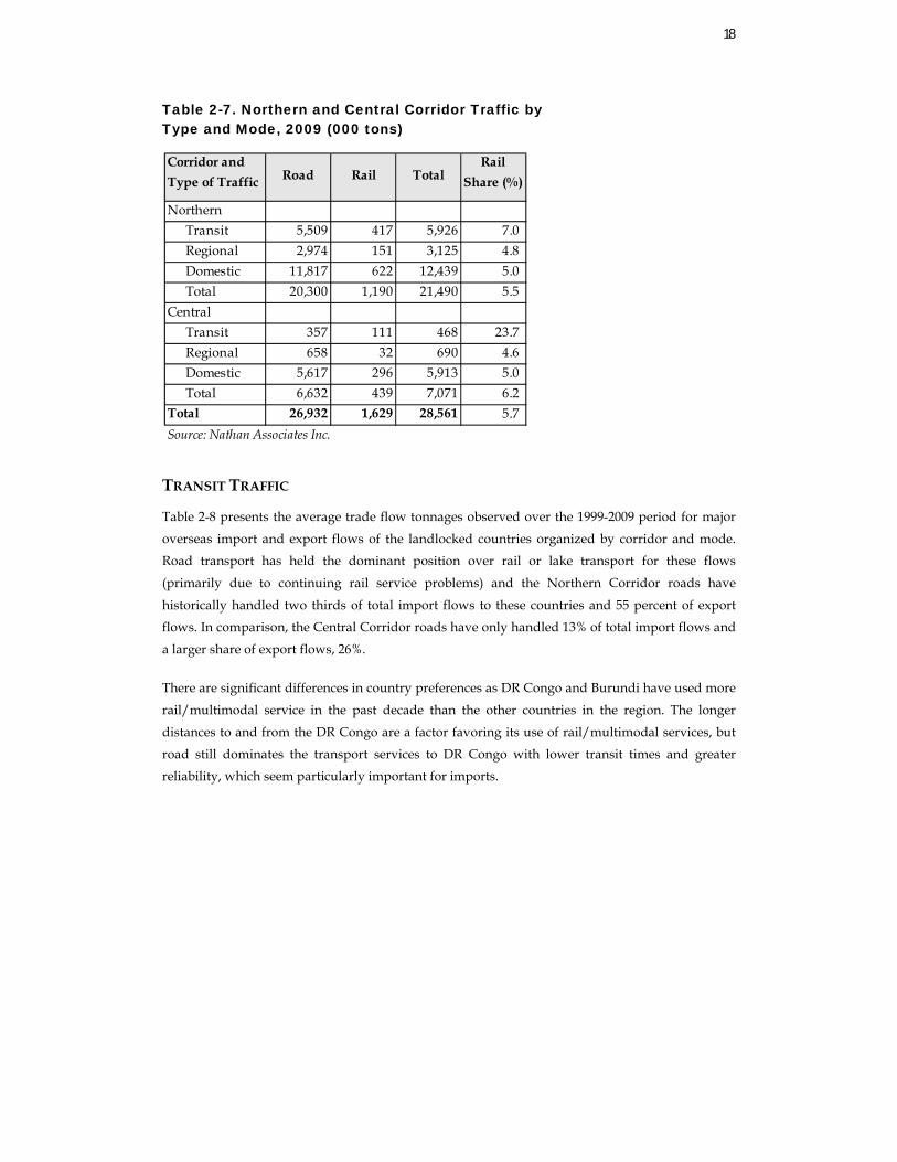
As presented in Table 2-7, total traffic on the Northern and Central Corridors in 2009 is estimated

at 28.6 million tons, of which 21.5 million tons were shipped via the Northern Corridor (75

percent) and 7.1 million tons on the Central Corridor (25 percent). More than 83 percent of the

traffic on the Central Corridor was domestic, that is, Tanzanian trade to overseas countries. Regional trade and transit traffic accounted for 10 percent and 7 percent, respectively of the

remaining Central Corridor traffic. On the Northern Corridor, Kenyan overseas trade accounted

for 58 percent of the total corridor traffic with transit traffic next at 28 percent and regional trade at 14 percent.

2005-2008 2005-2009

Burundi 103 177 212 270 335 37.9 34.3Eastern DRC 467 592 653 736 834 16.4 15.6Ethiopia 11 12 13 15 17 10.9 11.5Rwanda 244 320 371 487 550 25.9 22.5Sudan 141 130 145 220 156 16 2.6Uganda 2,449 2,578 3,151 3,471 3,730 12.3 11.1Total 3,416 3,809 4,546 5,199 5,622 15 13.3

Burundi 56 57 65 72 59 8.7 1.3Eastern DRC 63 77 98 122 145 24.6 23.2Ethiopia 30 35 40 45 50 14.5 13.6Rwanda 34 40 31 39 41 4.7 4.8Sudan 1 1 1 1 1 0 0Uganda 293 282 318 334 299 4.5 0.5Total 478 491 553 612 595 8.6 5.6

AAGR (%)

Imports

Exports

Country 2005 2006 2007 2008 2009

18

Table 2-7. Northern and Central Corridor Traffic by Type and Mode, 2009 (000 tons)

TRANSIT TRAFFIC

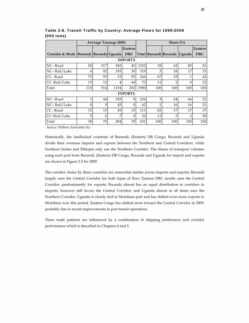
Table 2-8 presents the average trade flow tonnages observed over the 1999-2009 period for major

overseas import and export flows of the landlocked countries organized by corridor and mode. Road transport has held the dominant position over rail or lake transport for these flows

(primarily due to continuing rail service problems) and the Northern Corridor roads have

historically handled two thirds of total import flows to these countries and 55 percent of export flows. In comparison, the Central Corridor roads have only handled 13% of total import flows and

a larger share of export flows, 26%.

There are significant differences in country preferences as DR Congo and Burundi have used more

rail/multimodal service in the past decade than the other countries in the region. The longer

distances to and from the DR Congo are a factor favoring its use of rail/multimodal services, but

road still dominates the transport services to DR Congo with lower transit times and greater reliability, which seem particularly important for imports.

 

 

 

 

 

 

Corridor and Type of Traffic Road Rail Total

Rail Share (%)

NorthernTransit 5,509 417 5,926 7.0 Regional 2,974 151 3,125 4.8 Domestic 11,817 622 12,439 5.0 Total 20,300 1,190 21,490 5.5

CentralTransit 357 111 468 23.7 Regional 658 32 690 4.6 Domestic 5,617 296 5,913 5.0 Total 6,632 439 7,071 6.2

Total 26,932 1,629 28,561 5.7 Source: Nathan Associates Inc.

19

Burundi Rwanda UgandaEastern

DRC Burundi Rwanda UgandaEastern

DRC

20 317 942 43 1322 18 62 82 214 92 193 30 319 3 18 17 15

73 93 15 85 266 67 18 1 4213 12 4 44 73 11 2 0 22

110 514 1154 202 1980 100 100 100 100

1 44 183 8 236 3 64 64 210 9 45 8 62 1 16 16 21

32 15 49 15 111 83 17 17 375 2 7 8 22 13 3 2 20

38 70 284 39 431 100 100 100 100Source: Nathan Associates Inc.

EXPORTSNC - RoadNC– Rail/LakeCC - RoadCC- Rail/LakeTotal

Average Tonnage (000)

Total

Share (%)

Corridor & Mode

NC - RoadNC– Rail/LakeCC - RoadCC- Rail/LakeTotal

IMPORTS

Table 2-8. Transit Traffic by Country: Average Flows for 1999-2009 (000 tons)

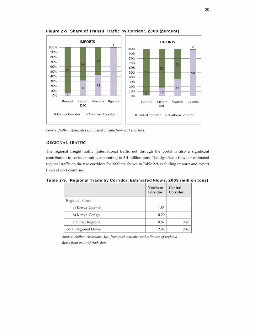
Historically, the landlocked countries of Burundi, (Eastern) DR Congo, Rwanda and Uganda

divide their overseas imports and exports between the Northern and Central Corridors, while

Southern Sudan and Ethiopia only use the Northern Corridor. The shares of transport volumes

using each port from Burundi, (Eastern) DR Congo, Rwanda and Uganda for import and exports

are shown in Figure 2-5 for 2009.

The corridor choice by these countries are somewhat similar across imports and exports; Burundi

largely uses the Central Corridor for both types of flow; Eastern DRC mostly uses the Central

Corridor, predominantly for exports; Rwanda almost has an equal distribution to corridors in

imports, however still favors the Central Corridor; and Uganda almost at all times uses the Northern Corridor. Uganda is closely tied to Mombasa port and has shifted even more exports to

Mombasa over this period. Eastern Congo has shifted more toward the Central Corridor in 2009,

probably due to recent improvements in port transit operations.

These trade patterns are influenced by a combination of shipping preferences and corridor

performance which is described in Chapters 4 and 5.

20

Figure 2-5. Share of Transit Traffic by Corridor, 2009 (percent)

Source: Nathan Associates Inc., based on data from port statistics.

REGIONAL TRAFFIC

The regional freight traffic (international traffic not through the ports) is also a significant

contribution to corridor traffic, amounting to 3.4 million tons. The significant flows of estimated

regional traffic on the two corridors for 2009 are shown in Table 2-9, excluding imports and export

flows of port countries.

Table 2-9. Regional Trade by Corridor: Estimated Flows, 2009 (million tons)

Northern Corridor

Central Corridor

Regional Flows

a) Kenya-Uganda 1.85 -

b) Kenya-Congo 0.20 -

c) Other Regional 0.87 0.46

Total Regional Flows 2.92 0.46

Source: Nathan Associates, Inc, from port statistics and estimates of regional flows from value of trade data.

21

3. Trade Demand Projections This chapter discusses the methodology used to obtain trade flow projections between country and overseas regional trading partners, through years 2009 to 2030. Then, additional trade from

major mining projects is discussed, focusing on important minerals for the region. Trade

projections are then used to forecast corridor traffic as described in Chapter 4.

Trade projections were prepared for the flows between eight countries of East Africa region, as

well as flows between East Africa countries and overseas regions for the years 2015 and 2030.

Trade values were obtained from IMF Direction of Trade Statistics and UN Comtrade for historical total trade between countries and regions. Trade projections were made using a regression

analysis, based on GDP and population projections. Consequently, we obtained future GDP and

population values and used them as inputs for the regression to obtain trade projections. In order to correct for possible aberrations resulting from the regressions, total imports and exports were

considered separately for countries. Trade totals were projected for each country in the East Africa

region, called control totals. Then, shares of trading partners over total trade were calculated and

applied to control totals in order to increase accuracy of results.

Methodology for Trade Projections

Trade projections for the East Africa region were prepared for 2015 and 2030 based upon a careful

review of historical data and a series of regression analysis using GDP and population as key

determinants. Projected flows of trade between the eight East African countries were prepared as

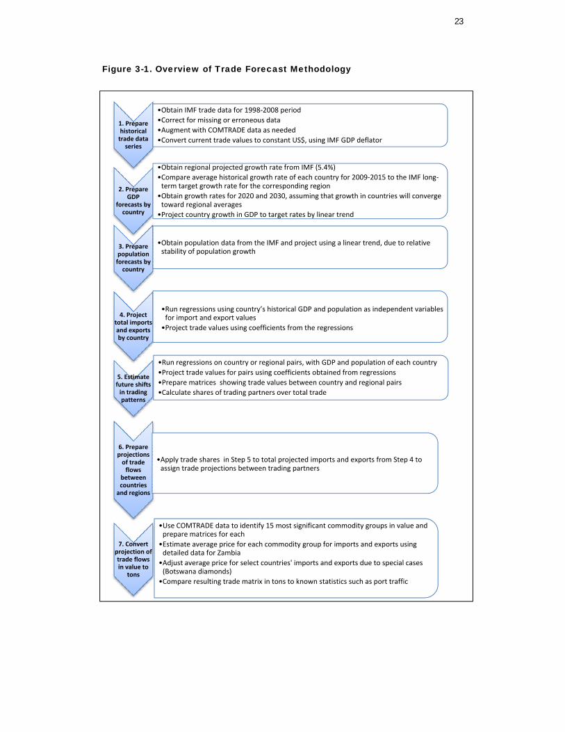
well as flows between the seven East African countries and six overseas regions7. The general approach for the preparation of the trade projections is presented in Figure 3-1. The approach

involved the following seven steps:

1. Prepare historical trade data series 2. Prepare GDP forecasts by country 3. Prepare population forecasts by country 4. Project total imports and exports by country 5. Estimate future shifts in trading patterns 6. Prepare projections of trade flows between countries and regions 7. Convert projection of trade flows in value to tons

7 East Asia, Europe, Latin America & Caribbean, Middle East, North America and South Asia.

22

1. PREPARE HISTORICAL TRADE DATA SERIES

As a first step, historical trade data for 1998-2008 in current US dollars was collected, reviewed and

cleaned for analysis. The primary source of trade data used in this analysis was the IMF Direction

of Trade Statistics as it is generally regarded as one of the more reliable sources of trade data. In

the case of missing or obvious erroneous data in the IMF series, we replaced the IMF data with

information obtained from the United Nations Statistics Division, Commodity Trade Statistics Database (COMTRADE). The resulting trade data series was converted to constant US dollars of

2008 by applying the IMF GDP deflator for each country.

Historical trends in trading patterns were described in Chapter 2.

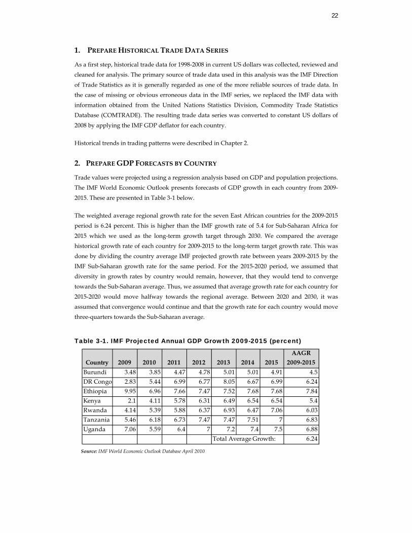
2. PREPARE GDP FORECASTS BY COUNTRY

Trade values were projected using a regression analysis based on GDP and population projections.

The IMF World Economic Outlook presents forecasts of GDP growth in each country from 2009-

2015. These are presented in Table 3-1 below.

The weighted average regional growth rate for the seven East African countries for the 2009-2015

period is 6.24 percent. This is higher than the IMF growth rate of 5.4 for Sub-Saharan Africa for

2015 which we used as the long-term growth target through 2030. We compared the average historical growth rate of each country for 2009-2015 to the long-term target growth rate. This was

done by dividing the country average IMF projected growth rate between years 2009-2015 by the

IMF Sub-Saharan growth rate for the same period. For the 2015-2020 period, we assumed that diversity in growth rates by country would remain, however, that they would tend to converge

towards the Sub-Saharan average. Thus, we assumed that average growth rate for each country for

2015-2020 would move halfway towards the regional average. Between 2020 and 2030, it was assumed that convergence would continue and that the growth rate for each country would move

three-quarters towards the Sub-Saharan average.

Table 3-1. IMF Projected Annual GDP Growth 2009-2015 (percent)

Source: IMF World Economic Outlook Database April 2010

Country 2009 2010 2011 2012 2013 2014 2015AAGR

2009-2015Burundi 3.48 3.85 4.47 4.78 5.01 5.01 4.91 4.5DR Congo 2.83 5.44 6.99 6.77 8.05 6.67 6.99 6.24Ethiopia 9.95 6.96 7.66 7.47 7.52 7.68 7.68 7.84Kenya 2.1 4.11 5.78 6.31 6.49 6.54 6.54 5.4Rwanda 4.14 5.39 5.88 6.37 6.93 6.47 7.06 6.03Tanzania 5.46 6.18 6.73 7.47 7.47 7.51 7 6.83Uganda 7.06 5.59 6.4 7 7.2 7.4 7.5 6.88

Total Average Growth: 6.24

23

1. Prepare historical trade data series

•Obtain IMF trade data for 1998‐2008 period•Correct for missing or erroneous data•Augment with COMTRADE data as needed•Convert current trade values to constant US$, using IMF GDP deflator

2. Prepare GDP 

forecasts by country

•Obtain regional projected growth rate from IMF (5.4%)•Compare average historical growth rate of each country for 2009‐2015 to the IMF long‐term target growth rate for the corresponding region•Obtain growth rates for 2020 and 2030, assuming that growth in countries will converge toward regional averages•Project country growth in GDP to target rates by linear trend

3. Prepare population forecasts by country

•Obtain population data from the IMF and project using a linear trend, due to relative stability of population growth 

4. Project total imports and exports by country

•Run regressions using country’s historical GDP and population as independent variables for import and export values •Project trade values using coefficients from the regressions

5. Estimate future shifts in trading patterns

•Run regressions on country or regional pairs, with GDP and population of each country•Project trade values for pairs using coefficients obtained from regressions•Prepare matrices  showing trade values between country and regional pairs•Calculate shares of trading partners over total trade

6. Prepare projections of trade flows 

between countries and regions

•Apply trade shares  in Step 5 to total projected imports and exports from Step 4 to assign trade projections between trading partners

7. Convert projection of trade flows in value to 

tons

•Use COMTRADE data to identify 15 most significant commodity groups in value and prepare matrices for each•Estimate average price for each commodity group for imports and exports using detailed data for Zambia•Adjust average price for select countries' imports and exports due to special cases (Botswana diamonds)•Compare resulting trade matrix in tons to known statistics such as port traffic

Figure 3-1. Overview of Trade Forecast Methodology

24

Overseas Region 2009-2015 2015-2020 2020-2030Europe 1.92 1.76 2.92North America 2.84 2.5 2.62Latin America & Caribbean

2.13 2.06 3.03

Middle East 2.63 5.31 4.77East Asia 8.36 9.23 8.6South Asia 4.82 5.87 6.86

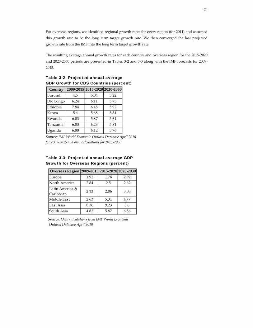
For overseas regions, we identified regional growth rates for every region (for 2011) and assumed

this growth rate to be the long term target growth rate. We then converged the last projected growth rate from the IMF into the long term target growth rate.

The resulting average annual growth rates for each country and overseas region for the 2015-2020

and 2020-2030 periods are presented in Tables 3-2 and 3-3 along with the IMF forecasts for 2009-

2015.

Table 3-2. Projected annual average GDP Growth for CDS Countries (percent)

Source: IMF World Economic Outlook Database April 2010 for 2009-2015 and own calculations for 2015-2030 Table 3-3. Projected annual average GDP Growth for Overseas Regions (percent)

Source: Own calculations from IMF World Economic Outlook Database April 2010

Country 2009-2015 2015-2020 2020-2030Burundi 4.5 5.04 5.22DR Congo 6.24 6.11 5.75Ethiopia 7.84 6.45 5.92Kenya 5.4 5.68 5.54Rwanda 6.03 5.87 5.64Tanzania 6.83 6.23 5.81Uganda 6.88 6.12 5.76

25

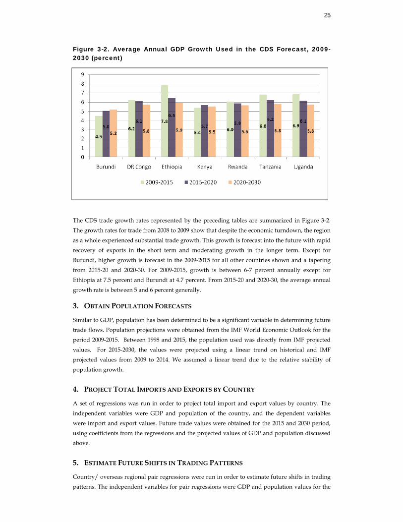
Figure 3-2. Average Annual GDP Growth Used in the CDS Forecast, 2009-2030 (percent)

The CDS trade growth rates represented by the preceding tables are summarized in Figure 3-2.

The growth rates for trade from 2008 to 2009 show that despite the economic turndown, the region

as a whole experienced substantial trade growth. This growth is forecast into the future with rapid recovery of exports in the short term and moderating growth in the longer term. Except for

Burundi, higher growth is forecast in the 2009-2015 for all other countries shown and a tapering

from 2015-20 and 2020-30. For 2009-2015, growth is between 6-7 percent annually except for

Ethiopia at 7.5 percent and Burundi at 4.7 percent. From 2015-20 and 2020-30, the average annual

growth rate is between 5 and 6 percent generally.

3. OBTAIN POPULATION FORECASTS

Similar to GDP, population has been determined to be a significant variable in determining future trade flows. Population projections were obtained from the IMF World Economic Outlook for the

period 2009-2015. Between 1998 and 2015, the population used was directly from IMF projected

values. For 2015-2030, the values were projected using a linear trend on historical and IMF projected values from 2009 to 2014. We assumed a linear trend due to the relative stability of

population growth.

4. PROJECT TOTAL IMPORTS AND EXPORTS BY COUNTRY

A set of regressions was run in order to project total import and export values by country. The

independent variables were GDP and population of the country, and the dependent variables

were import and export values. Future trade values were obtained for the 2015 and 2030 period,

using coefficients from the regressions and the projected values of GDP and population discussed above.

5. ESTIMATE FUTURE SHIFTS IN TRADING PATTERNS

Country/ overseas regional pair regressions were run in order to estimate future shifts in trading

patterns. The independent variables for pair regressions were GDP and population values for the

26

trading partners8, with the dependent variables being import and export values. Trade values for

pairs were projected using regression coefficients. Regression results were checked and re-structured when needed. In order to optimize statistical significance levels and eliminate

occasional extreme trends in results, in some cases regressions were run with fewer data points

(years) and at other times by aggregating the country variables within the region to a single

variable representing the regional GDP and population. The results of the pair analysis were

compiled into trade matrices for 2015 and 2030 showing trade flows between country and regional

pairs. The trade matrix was then converted into trade flow shares for each trading partner pair by dividing trade for each pair by the total trade in the trade flow matrix.

6. PREPARE PROJECTIONS OF TRADE FLOWS BETWEEN COUNTRIES AND REGIONS

The trade shares resulting from the pair analysis in Step 5 above were then applied to the total

projected imports and exports from Step 4 to obtain trade projections for the selected year between

trading partners.

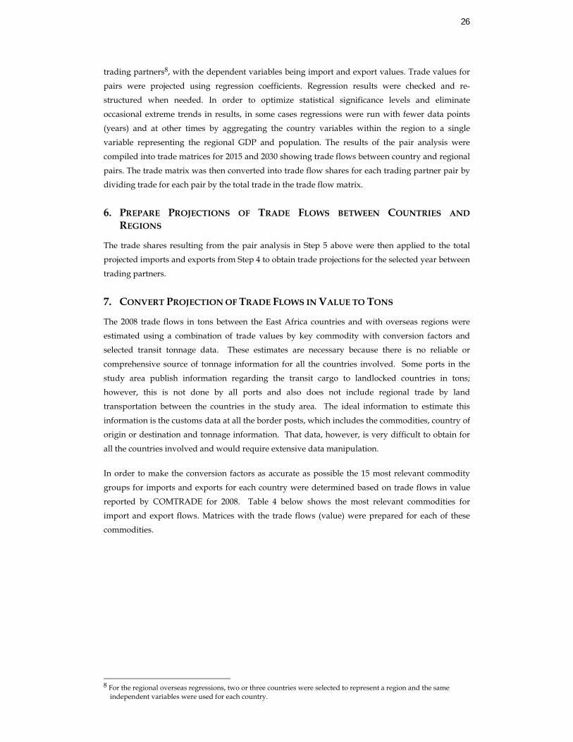
7. CONVERT PROJECTION OF TRADE FLOWS IN VALUE TO TONS

The 2008 trade flows in tons between the East Africa countries and with overseas regions were

estimated using a combination of trade values by key commodity with conversion factors and selected transit tonnage data. These estimates are necessary because there is no reliable or

comprehensive source of tonnage information for all the countries involved. Some ports in the

study area publish information regarding the transit cargo to landlocked countries in tons; however, this is not done by all ports and also does not include regional trade by land

transportation between the countries in the study area. The ideal information to estimate this

information is the customs data at all the border posts, which includes the commodities, country of origin or destination and tonnage information. That data, however, is very difficult to obtain for

all the countries involved and would require extensive data manipulation.

In order to make the conversion factors as accurate as possible the 15 most relevant commodity

groups for imports and exports for each country were determined based on trade flows in value

reported by COMTRADE for 2008. Table 4 below shows the most relevant commodities for

import and export flows. Matrices with the trade flows (value) were prepared for each of these commodities.

8 For the regional overseas regressions, two or three countries were selected to represent a region and the same

independent variables were used for each country.

27

Commodity Factor ($/ton)Cereals 372Vegetable Oils 930Ores 112Oil and Fuel 506Org Chemicals 2,508Pharmaceutical 24,511Fertilisers 844Plastics 2,358Precious Stones, gold 18,849Iron and steel 1,272Articles of iron or steel 3,148Mechanical appliances 5,616Electrical machinery & equipment 3,388Vehicles and parts 1,731Optical & precision instruments 23,767

IMPORTS

Table 3-4. Conversion Factors for Commodities Used to obtain Tonnages

Source: Nathan Associates Inc.

The next step was to estimate commodity group-specific conversion factors for imports and

exports using the most relevant commodity groups identified in the previous step. The commodity

group conversion values were compared against value and tonnage information obtained for

Rwanda, Burundi and Uganda and further adjustments made to conversion factors for country

pairs that showed larger than expected flows that indicate a concentration higher than normal of a more expensive commodity within a commodity group.

Once the trade matrices of the selected commodity groups are aggregated for a given country, the

difference between the total country trade flows and the total of the selected commodity groups is designated “other” commodities. The goal is that the selected commodities represent most of the

country trade and as a result the “other” category is relatively small, increasing the accuracy of the

analysis.

We then estimated 2008 trade flows in tons for the selected commodity groups using the

calculated conversion factors for each commodity. For the “others” category we used an average

factor of overall conversion factor for imports and exports. The aggregation of the respective

matrices gives a rough estimate of 2008 Trade Flows in tons. This estimate was further refined by

adjusting tonnage flows for overseas partners to match known port trade flows and regional flows

in tons.

Finally, we estimated conversion factors by country and overseas regional pairs that reflect the

current commodity mix by dividing the 2008 Total Trade matrix (value) over estimated 2008 Total

Trade matrix (tons). These factors were then used for the trade projections for 2015 and 2030.

Commodity Factor ($/ton)Fish 3,317Tea/Coffee 2,471Sugar 483Tobacco 1,885Oil/Coal 506Cotton 1,530Textiles 414Textiles 6,807Textiles 13,595Diamonds/Gold 18,849Iron 1,272Copper 3,172Nickel 56Manganese 37,810

EXPORTS

28

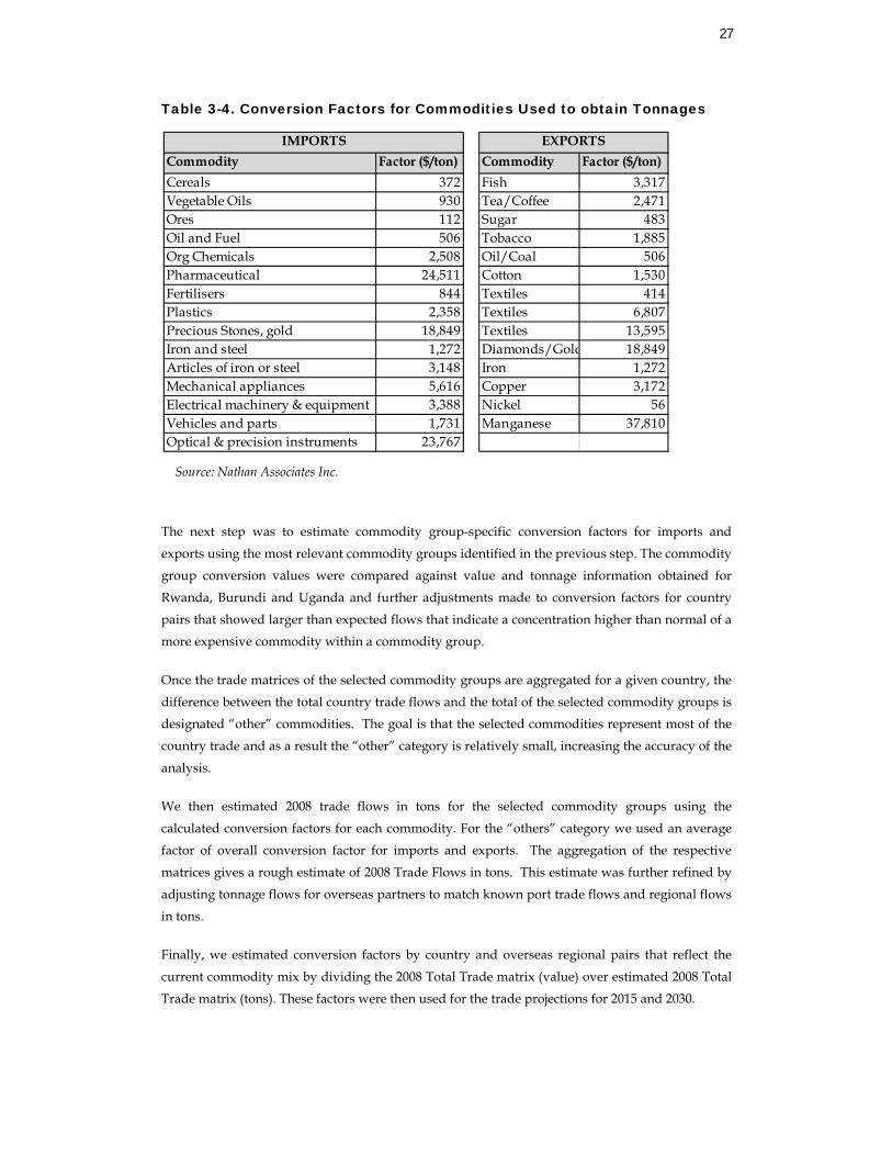
Results of Trade Projections Despite the economic turndown in 2009, the region as a whole experienced substantial trade

growth. This growth is forecast into the future with rapid recovery of exports in the short term and moderating growth in the longer term. The CDS trade growth rates are summarized in Table 3-6.

High growth rates in both imports and exports are observed in the upcoming period 2009-2015.

The regional annual average growth rates for imports in this period is expected to be 11.9%, while the average for exports is expected at 10.9%. Burundi and Eastern DRC are expected to have

import growth at around 16%, followed by Rwanda and Kenya. Highest growth in exports is

expected to be in Sudan (although from a very low base) and Rwanda (23.3%). Growth is expected

to slow down in the period 2015-2030 in relation to the upcoming period, however regional

averages still display relatively high rates in our forecasts: 6.1% for imports and 8.2% for exports.

Table 3-6. East Africa Average Annual Growth Rates of Imports and Exports (percent)

Country 2009-2015 2015-2030 Imports Exports Imports Exports

Burundi 16.5 19.6 3.2 6.6

Eastern DRC 16.0 13.6 7.2 13.4

Ethiopia 6.1 3.5 0.9 13.1

Kenya 13.0 7.2 6.8 4.6

Rwanda 14.4 23.3 6.1 12.2

Sudan 5.0 66.1* 5.0 5.0

Tanzania 11.2 12.7 7.1 6.7

Uganda 10.6 13.6 4.1 5.5

Total 11.9 10.9 6.1 8.2

* Trade with Kenya and Tanzania only growth, from a small base

Source: Tables 3-6 and3-7.

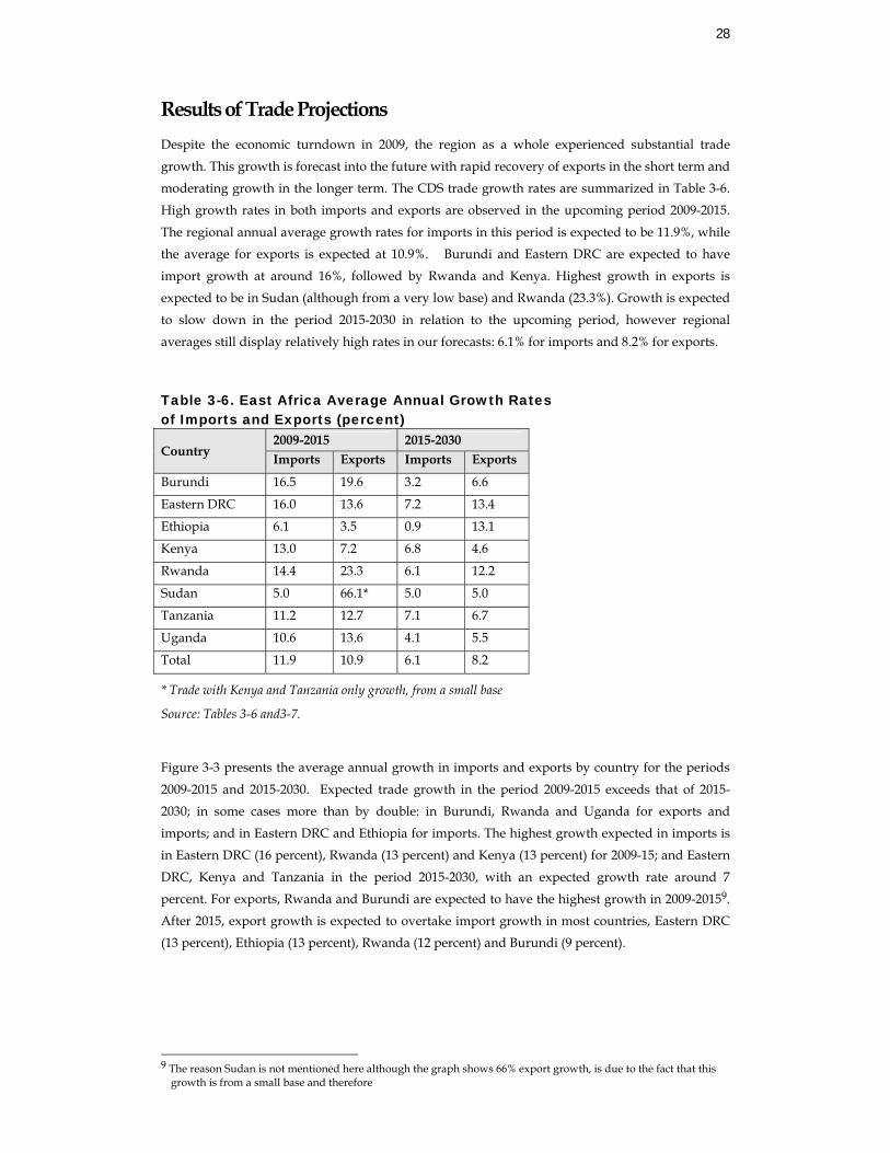
Figure 3-3 presents the average annual growth in imports and exports by country for the periods

2009-2015 and 2015-2030. Expected trade growth in the period 2009-2015 exceeds that of 2015-2030; in some cases more than by double: in Burundi, Rwanda and Uganda for exports and

imports; and in Eastern DRC and Ethiopia for imports. The highest growth expected in imports is

in Eastern DRC (16 percent), Rwanda (13 percent) and Kenya (13 percent) for 2009-15; and Eastern

DRC, Kenya and Tanzania in the period 2015-2030, with an expected growth rate around 7

percent. For exports, Rwanda and Burundi are expected to have the highest growth in 2009-20159.

After 2015, export growth is expected to overtake import growth in most countries, Eastern DRC (13 percent), Ethiopia (13 percent), Rwanda (12 percent) and Burundi (9 percent).

9 The reason Sudan is not mentioned here although the graph shows 66% export growth, is due to the fact that this

growth is from a small base and therefore

29

Figure 3-3. Average Annual Trade Growth by Country, 2009-2015 and 2015-2030 (percent)

2009-2015

*The value for Sudan Exports (66%) is not to scale

2015-2030

Source: Nathan Associates Inc.

Potential for Additional Trade from Major Mining Projects

In addition to the trade figures presented above, there are several major mining projects that can

generate substantially further trade flows over the next two decades. These development projects

are normally seen as anchors for additional transportation projects.

MINERALS SECTOR OVERVIEW

In this section, we review minerals mined or extracted in eastern African that are highly

dependent on the transport sector for inputs and outputs. Transport demand from the minerals

very often provides anchor projects to justify major infrastructure investment and developments.

There is a common perception that provision of transport infrastructure leads directly to new

mining projects, but it is almost always the other way around: the decision to proceed with a

mining project, based on estimated or calculated logistics costs, is the basis for infrastructure

financing. For example, the construction of a standard gauge railway on the Central Corridor will

not necessarily lead to implementation of planned nickel mining ventures. Governments can

decide to invest in road, railway, and port projects on the basis of projected economic and social

30

benefits. The private sector, however, will only invest on the basis of agreed contracts and/or

income guarantees. Failure to take this into account is one of the main reasons for the general collapse of the railway concessions, despite the terms of the concession agreement and the

commitments made. Thus the infrastructure investments required to serve various planned

mining projects—coal, iron ore, nickel, mineral sands—will have to be preceded by a decision to

proceed with the mining projects and the willingness to enter into a long-term transport contracts.

Copper. The main producer is the Zambia copper belt, with current production of 0.7 mtpa,

increasing to 1.2 mtpa of copper metal, mostly transported by road to Durban via South Africa, a distance of 3,000 km at about US$ 180/ton. About 0.2 mtpa goes by rail via Dar es Salaam, about

2,000 km at US$ 100/ton. The DRC production of about 0.2 mtpa, increasing to an estimated 0.5

mtpa, will likely mostly go via Lobito by rail after 2011. Possible new railway links from Lumwana/Solwezi to Chingola and Kolwezi will change traffic patterns. The previous inter-mine

railway traffic, about 1 mtpa, is now all by road. Transport by rail to Dar es Salaam and to Lobito

seems to be the most likely long term scenario.

Iron Ore. The only regional iron ore project that could affect transport demand in the East Africa

Region is the Mt. Kodo iron deposit in eastern DRC. The railway distance to the nearest port is

about 1,800 km, either Mombasa or a new port at Lamu. Very large volumes will be required, up

to 50 mtpa, to achieve low railway tariffs of the order of US$ 30/ton or less, and very low interest

financing will be required for financial viability of the railway. If a long-term contract at today’s

high iron ore prices could be secured this project could be viable. This will require a new rather than an upgraded railway alignment, which will bring major regional economic benefits.

Nickel. Nickel is produced together with copper in smaller quantities, using the same transport

methods. It seems likely, on the basis of recent feasibility studies, that several major nickel mines will be established in Burundi and north western Tanzania, and these will serve as anchor projects

for upgrading or building a railway line on the Central Corridor. Transport volumes will depend

on the degree of processing required. It seems most likely that the export product will be nickel

concentrate, from 200,000 to 700 000 tpa, exported by rail to Dar es Salaam, with a tariff of about

US$ 60/ton over a distance of more than 1,000 km. The value of the nickel concentrate will likely

vary between US$ 3,000 and US$ 5,000/ton, depending on the percent concentration and the nickel metal price, which was high at US$26,000/ton in April 2010, but also volatile.

Other--Precious metals, oil. The main transport demand from gold and diamond mining

operations relates to inputs, mainly fuel, consumables, processing chemicals, and heavy equipment. Volumes depend on the size of the mining operations and can be considerable. Inputs

for a very large mining operation could fill one to two trains per day, or 200,000 to 500,000 tpa or

up to 50 road trucks per day, excluding fuel imports. The very high cost of transporting heavy industrial equipment by road, mainly as a result of a “road damage compensation fee” is a major

development constraint, particularly in Tanzania.

31

Additional details for those mining projects that will have the greatest potential impact on the

Northern and Central corridors (iron ore and nickel) are presented below:10

Iron Ore

Location. The main iron ore deposits in Africa are in South Africa, Liberia, and Eastern DRC.

Those in the DRC are not yet being mined. In relation to the Northern Corridor, the DRC deposits

at Mt. Kodo close to Lake Albert are of interest, because they could provide an anchor project for a

rail and port terminal system for exports through Mombasa or Lamu. The total world production

of iron ore is about 1,700 million tpa, of which about 50 percent is carried by seaborne trade.

Preliminary studies indicate that the Mt. Kodo deposit could yield exports of up to 50 mtpa (ref Northern Corridor SDI study).

Process and Products. Iron ore is sold as lumpy ore and fines, with a benchmark of 63.5 percent

iron content. Processing may include crushing, grinding, and gravity or magnetic separation to achieve the desired iron content. Further processing could include the production of direct

reduced iron (DRI), using gas or coke to reduce the iron ore to achieve and iron content of more

than 90 percent, and to obtain higher prices and to reduce transport sensitivity.

Mining Activity and Marketing. There is no mining at Mt. Kodo, but Chinese steel producers are

interested, subject to the provision of transport infrastructure and acceptable transport costs. It

seems likely that the Chinese market could accept 50 mtpa. A long-term export contract (10+

years) would be required to secure financing for mining and transport infrastructure.

Transport Demand and Infrastructure. Large volumes of iron ore, typically tens of millions of tons

per annum, cannot be transported economically by road over long distances. Ore is traditionally carried by heavy haul rail at very low unit prices, less than US$0.02 per ton-km (less than the cost

of fuel by road) in dedicated wagons, and shipped in very large bulk carriers (Cape Size vessels,

more than 120,000 DWT), requiring special bulk port terminals with a quayside depth and port access depth of more than 18m (for example, Saldanha Bay port in South Africa . Mombasa port

has a depth of 10m, but is being upgraded to 15 m. The rail distance from the eastern DRC to

Mombasa is about 1700 km.

Prices and Transport Sensitivity. Iron ore is traded at US$183/ton C&F China port (April 2010),

up from US$ 132/ton in February 2010, and up from about US$70/ton in 2006. It seems unlikely

that long-term supply contracts will exceed US$80 to 100/ton C&F—there is no shortage of iron

ore reserves, only a current mining capacity constraint. Bulk ocean freight rates vary considerably

according to demand, but tend to correct fairly quickly with market response. Assuming a

shipping freight rate of US$ 15/ton, a port handling cost of US$ 4/ton, and a railway tariff of US$ 45/ton, would yield a unit tariff of US$ 0.025 per tkm over a distance of 1,800 km. Transport costs

are therefore likely to make up to 80 percent of the C&F price of the iron ore, which is unlikely to

be a viable operation in the short to medium term. The South African iron ore exports have a rail distance of about 860 km to Saldanha Bay.

10 The copper mining projects in Zambia will affect the demand on the Dar Corridor and must be considered for the

future performance of the port of Dar es Salaam.

32

Nickel

Location. Nickel is produced as part of most copper production. Big nickel deposits have been

discovered and explored in Burundi (Musongati, Waga, Nyabekere) and in north western

Tanzania, with a potential production of nickel concentrates of more than 700,000 tpa. It is most

likely that this will be exported through Dar es Salaam via the Central Corridor railway system,

which will require upgrading or replacement with a new standard gauge railway.

Mining Activity and Marketing. The most significant potential development is the likely start up

of mining projects in Burundi and Tanzania though the decision to proceed has not yet been made

and will depend on the provision of suitable transport infrastructure, mainly railway upgrades and extensions on the Central Corridor.

Process and Products. Nickel deposits are found mostly as sulphide deposits or as laterite

deposits. Sulphide ores are treated by roasting and reduction processes to produce a nickel matte with about 75 percent nickel. Further purification is often by leaching and electro-winning –

adequate electricity supply in remote regions is often a constraint.

Transport Demand and Infrastructure. Nickel ores and nickel concentrates are ideally transported by rail, whereas the pure metal, with a typical value of US$15,000 to US$28,000/t is not transport

sensitive, and more likely to be transported by road. The proposed new standard gauge railway on

the Central Corridor is partly based on the projected traffic from the planned nickel mines, but

with a projected demand of less than 1mtpa (depending on whether ore or concentrates are to be

transported) is unlikely to make the new standard gauge railway viable without another anchor

project as well.

Prices and Transport Sensitivity. Nickel metal prices are highly variable, between US$18,900 to

$26,000/ton from February to April 2010. The question of transport demand depends on the

degree of processing at the mine—whether it is large volume of low priced ore, or a much lower volume of high priced concentrate or matte. The feasibility of the nickel mining project will have to

be established, and a decision to proceed made, before the related infrastructure upgrades and

extensions can be financed.

Iron, nickel and copper concentrates are likely to move in the two corridors in the future.

Movements of equipment for operations and other imports to support these developments would

accompany this development. This movement may be closely tied to rail system developments.

33

4. Traffic Forecasts and Corridor / Mode Allocation

In this chapter we discuss how estimated trade forecast values are assigned to each corridor and mode. We then consider the potential impact of proposed projects on corridor performance and

reallocate traffic based on new performance parameters. We present the resulting traffic forecasts

as a Base Case scenario; which is defined as an improved and unconstrained scenario.

Methodology

STATUS QUO SCENARIO

Corridor choice depends on the following factors: corridor performance from an importer or exporter’s point of view; ship service for overseas trade and any preferences of the shipper for a

specific transit country or port. Performance is determined by price, time and reliability for

shipping via a given corridor and/or mode. These data were gathered for the Northern and Central Corridors for 2010, and analyzed using our Fast Path model11.

Based on statistical analysis of historic trade data by corridor and mode as well as performance

data, a Corridor and Mode Choice Model was developed. Socioeconomic and policy indicators

were also taken into account as factors of this model. The model produces shares for each

country/region trading pair on the expected distribution of trade between corridors and modes.

These shares are then multiplied by the trade volumes in an allocation model, which in turn aggregates individual flows into corridors and modes for status quo traffic forecasts.

Status quo scenario implies that the performance parameters of the corridors will remain

unaltered; they will neither improve nor deteriorate. The corridor would undergo regular upgrades, maintenance and expansion that would preserve current performance parameters but

no projects are assumed to be planned, which could improve price, time or reliability conditions of

the corridor. At the end of this process, we would have corridor and mode shares for all possible transport alternatives for each country.

11 See CDS Technical Paper entitled “Corridor Diagnostic Audit and Results” for more details.

34

BASE CASE SCENARIO

It would not be realistic to leave the traffic forecasts at the status quo scenario, since proposed

projects to improve the Northern and Central Corridors actually exist. Therefore, we considered a

second scenario, named “Base Case scenario”, which takes into account the possible diversion in

traffic due to improvements from proposed projects and is assumed to be unconstrained in terms

of capacity.

For the Base Case scenario, we first had to identify the potential impact of proposed projects on

corridor performance parameters; namely price, cost and reliability. For this, the new estimated

parameters for road, rail segments and ports were coded into FastPath, which produced corridor level aggregate performance parameters. These were compared against the status quo baseline to

estimate impact.

Based on the improved performance parameters of corridors, the traffic assignment to different corridors and modes would shift. Incorporating the estimated impact of new performance

parameters, corridor and mode shares are recalculated for the Base Case scenario; once again

using the Corridor and Mode Choice Model. The new shares are applied to future trade values in

order to estimate the traffic allocation of corridors and modes for years 2015 and 2030.

The corridor and mode choice analysis is unconstrained since it does not take into account any

capacity constraints which would limit the flows. This is based on the assumption that capacity

additions will be implemented to meet demand.

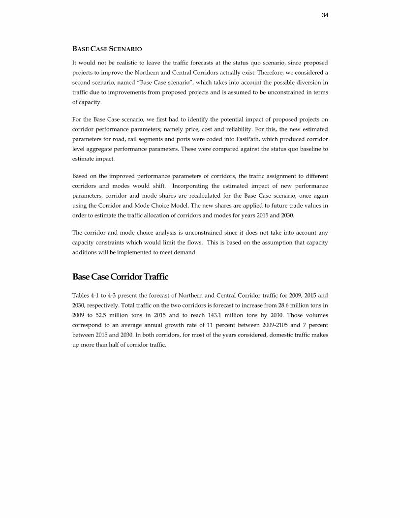
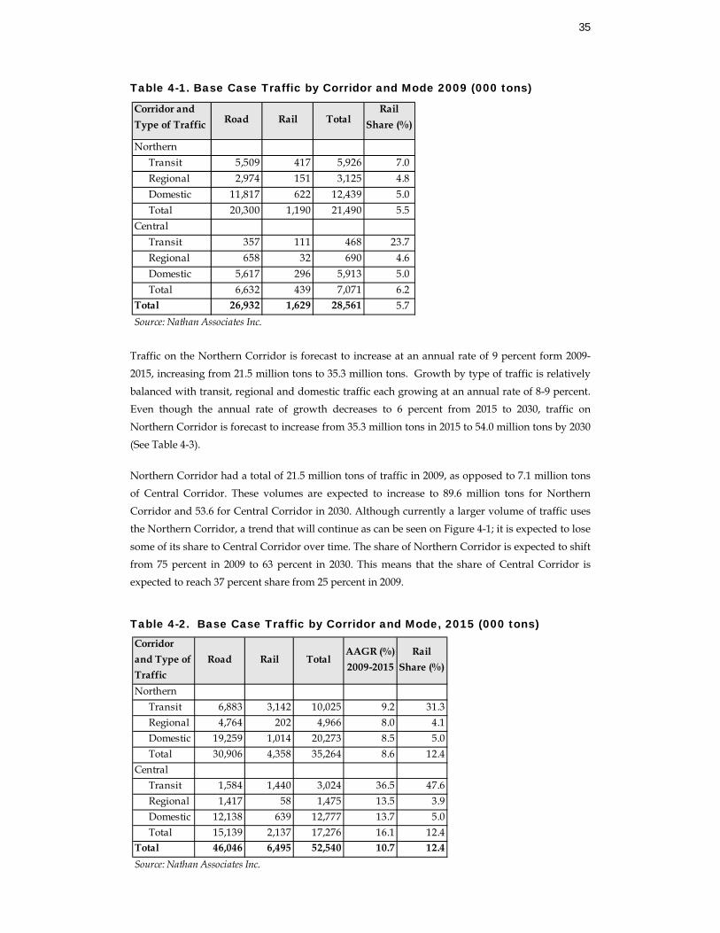
Base Case Corridor Traffic

Tables 4-1 to 4-3 present the forecast of Northern and Central Corridor traffic for 2009, 2015 and

2030, respectively. Total traffic on the two corridors is forecast to increase from 28.6 million tons in

2009 to 52.5 million tons in 2015 and to reach 143.1 million tons by 2030. Those volumes correspond to an average annual growth rate of 11 percent between 2009-2105 and 7 percent

between 2015 and 2030. In both corridors, for most of the years considered, domestic traffic makes

up more than half of corridor traffic.

35

Corridor and Type of Traffic

Road Rail TotalAAGR (%) 2009-2015

Rail Share (%)

NorthernTransit 6,883 3,142 10,025 9.2 31.3Regional 4,764 202 4,966 8.0 4.1Domestic 19,259 1,014 20,273 8.5 5.0Total 30,906 4,358 35,264 8.6 12.4

CentralTransit 1,584 1,440 3,024 36.5 47.6Regional 1,417 58 1,475 13.5 3.9Domestic 12,138 639 12,777 13.7 5.0Total 15,139 2,137 17,276 16.1 12.4

Total 46,046 6,495 52,540 10.7 12.4Source: Nathan Associates Inc.

Table 4-1. Base Case Traffic by Corridor and Mode 2009 (000 tons)

Traffic on the Northern Corridor is forecast to increase at an annual rate of 9 percent form 2009-

2015, increasing from 21.5 million tons to 35.3 million tons. Growth by type of traffic is relatively

balanced with transit, regional and domestic traffic each growing at an annual rate of 8-9 percent. Even though the annual rate of growth decreases to 6 percent from 2015 to 2030, traffic on

Northern Corridor is forecast to increase from 35.3 million tons in 2015 to 54.0 million tons by 2030

(See Table 4-3).

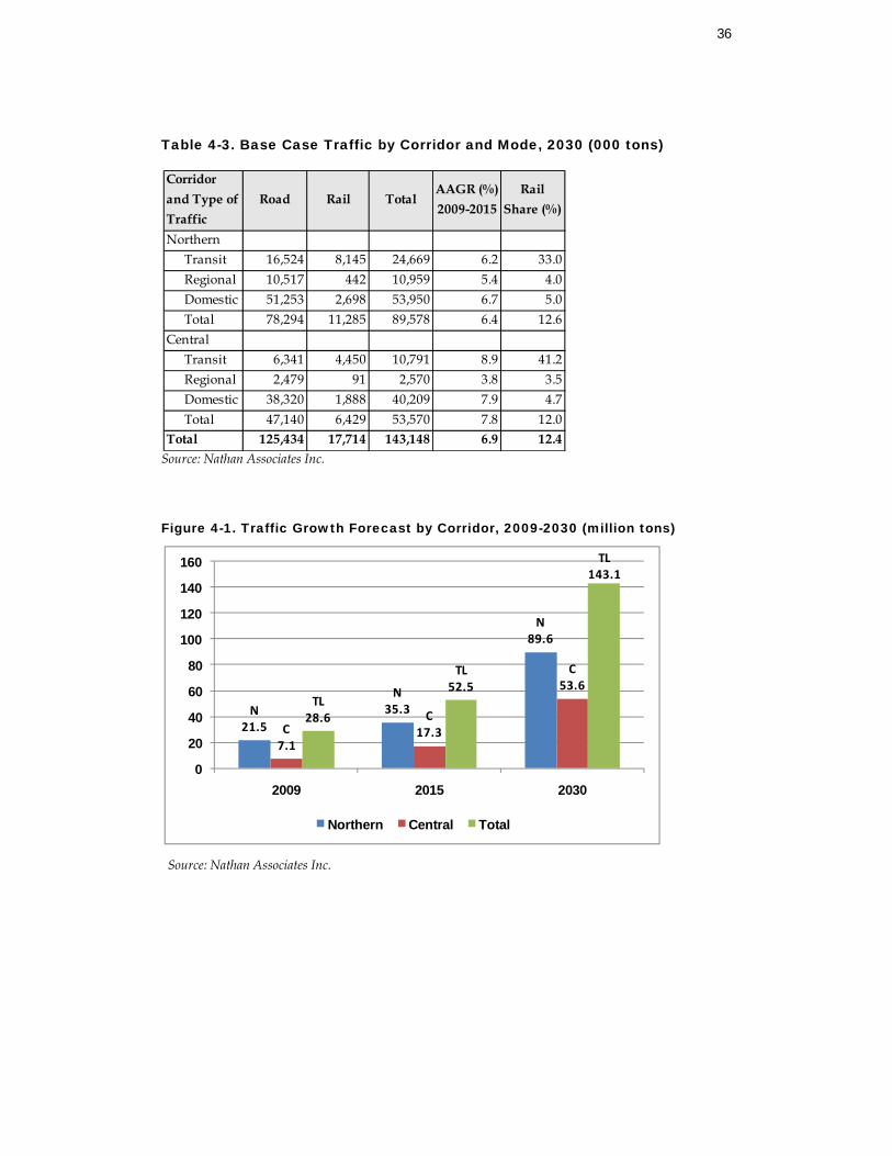
Northern Corridor had a total of 21.5 million tons of traffic in 2009, as opposed to 7.1 million tons

of Central Corridor. These volumes are expected to increase to 89.6 million tons for Northern

Corridor and 53.6 for Central Corridor in 2030. Although currently a larger volume of traffic uses the Northern Corridor, a trend that will continue as can be seen on Figure 4-1; it is expected to lose

some of its share to Central Corridor over time. The share of Northern Corridor is expected to shift

from 75 percent in 2009 to 63 percent in 2030. This means that the share of Central Corridor is expected to reach 37 percent share from 25 percent in 2009.

Table 4-2. Base Case Traffic by Corridor and Mode, 2015 (000 tons)

Corridor and Type of Traffic Road Rail Total

Rail Share (%)

NorthernTransit 5,509 417 5,926 7.0 Regional 2,974 151 3,125 4.8 Domestic 11,817 622 12,439 5.0 Total 20,300 1,190 21,490 5.5

CentralTransit 357 111 468 23.7 Regional 658 32 690 4.6 Domestic 5,617 296 5,913 5.0 Total 6,632 439 7,071 6.2

Total 26,932 1,629 28,561 5.7 Source: Nathan Associates Inc.

36

N21.5

N35.3

N89.6

C7.1

C17.3

C53.6

TL28.6

TL52.5

TL143.1

0

20

40

60

80

100

120

140

160

2009 2015 2030

Northern Central Total

Table 4-3. Base Case Traffic by Corridor and Mode, 2030 (000 tons)

Source: Nathan Associates Inc.

Figure 4-1. Traffic Growth Forecast by Corridor, 2009-2030 (million tons)

Source: Nathan Associates Inc.

Corridor and Type of Traffic

Road Rail TotalAAGR (%) 2009-2015

Rail Share (%)

NorthernTransit 16,524 8,145 24,669 6.2 33.0Regional 10,517 442 10,959 5.4 4.0Domestic 51,253 2,698 53,950 6.7 5.0Total 78,294 11,285 89,578 6.4 12.6

CentralTransit 6,341 4,450 10,791 8.9 41.2Regional 2,479 91 2,570 3.8 3.5Domestic 38,320 1,888 40,209 7.9 4.7Total 47,140 6,429 53,570 7.8 12.0

Total 125,434 17,714 143,148 6.9 12.4

37

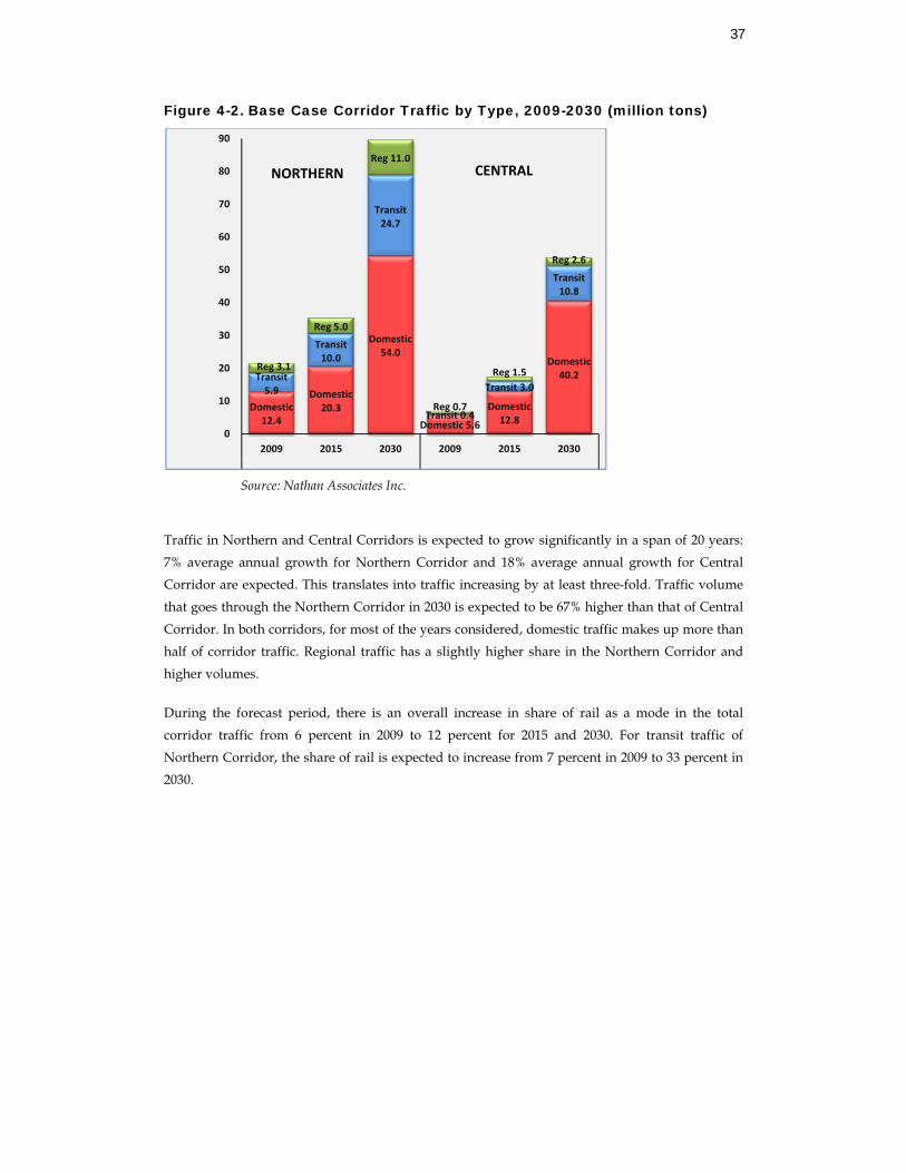
Figure 4-2. Base Case Corridor Traffic by Type, 2009-2030 (million tons)

Source: Nathan Associates Inc.

Traffic in Northern and Central Corridors is expected to grow significantly in a span of 20 years:

7% average annual growth for Northern Corridor and 18% average annual growth for Central

Corridor are expected. This translates into traffic increasing by at least three-fold. Traffic volume

that goes through the Northern Corridor in 2030 is expected to be 67% higher than that of Central

Corridor. In both corridors, for most of the years considered, domestic traffic makes up more than

half of corridor traffic. Regional traffic has a slightly higher share in the Northern Corridor and

higher volumes.

During the forecast period, there is an overall increase in share of rail as a mode in the total

corridor traffic from 6 percent in 2009 to 12 percent for 2015 and 2030. For transit traffic of

Northern Corridor, the share of rail is expected to increase from 7 percent in 2009 to 33 percent in

2030.

Domestic12.4

Domestic20.3

Domestic54.0

Domestic 5.6

Domestic12.8

Domestic40.2Transit

5.9

Transit10.0

Transit24.7

Transit 0.4

Transit 3.0

Transit10.8

Reg 3.1

Reg 5.0

Reg 11.0

Reg 0.7

Reg 1.5

Reg 2.6

0

10

20

30

40

50

60

70

80

90

2009 2015 2030 2009 2015 2030

CENTRALNORTHERN

38

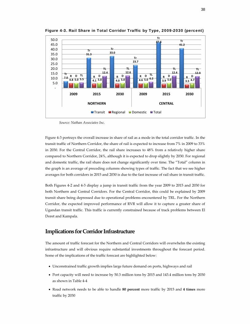
Figure 4-3. Rail Share in Total Corridor Traffic by Type, 2009-2030 (percent)

Source: Nathan Associates Inc.

Figure 4-3 portrays the overall increase in share of rail as a mode in the total corridor traffic. In the

transit traffic of Northern Corridor, the share of rail is expected to increase from 7% in 2009 to 33%

in 2030. For the Central Corridor, the rail share increases to 48% from a relatively higher share

compared to Northern Corridor, 24%, although it is expected to drop slightly by 2030. For regional

and domestic traffic, the rail share does not change significantly over time. The “Total” column in

the graph is an average of preceding columns showing types of traffic. The fact that we see higher

averages for both corridors in 2015 and 2030 is due to the fast increase of rail share in transit traffic.

Both Figures 4-2 and 4-3 display a jump in transit traffic from the year 2009 to 2015 and 2030 for

both Northern and Central Corridors. For the Central Corridor, this could be explained by 2009

transit share being depressed due to operational problems encountered by TRL. For the Northern

Corridor, the expected improved performance of RVR will allow it to capture a greater share of

Ugandan transit traffic. This traffic is currently constrained because of track problems between El

Doret and Kampala.

Implications for Corridor Infrastructure

The amount of traffic forecast for the Northern and Central Corridors will overwhelm the existing

infrastructure and will obvious require substantial investments throughout the forecast period.

Some of the implications of the traffic forecast are highlighted below:

• Unconstrained traffic growth implies large future demand on ports, highways and rail

• Port capacity will need to increase by 50.3 million tons by 2015 and 143.4 million tons by 2030

as shown in Table 4-4

• Road network needs to be able to handle 80 percent more traffic by 2015 and 4 times more

traffic by 2030

Tr7.0 

Tr 31.3 

Tr33.0 

Tr23.7 

Tr47.6  Tr

41.2 

R4.8 

R4.1 

R4.0 

R4.6 

R3.9 

R3.5 

D5.0 

D5.0 

D5.0 

D5.0 

D5.0 

D4.7 

TL5.5 

TL12.4 

TL12.6 

TL6.2 

TL12.4 

TL12.0 

‐5.0 

10.0 15.0 20.0 25.0 30.0 35.0 40.0 45.0 50.0 

2009 2015 2030 2009 2015 2030

NORTHERN CENTRAL

Transit Regional Domestic Total

39

• If capacity is not increased, congestion at ports and on roads will reach epic levels and

constrain economic growth

There is a clear need for substantial and targeted investment in regional transport infrastructure

now and continuing for the next several decades.

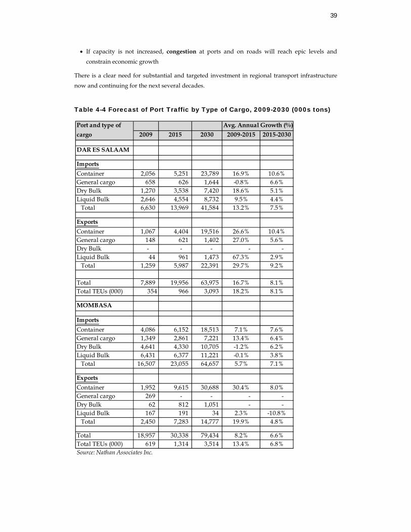
Table 4-4 Forecast of Port Traffic by Type of Cargo, 2009-2030 (000s tons)

Avg. Annual Growth (%)2009 2015 2030 2009-2015 2015-2030

DAR ES SALAAM

ImportsContainer 2,056 5,251 23,789 16.9% 10.6%General cargo 658 626 1,644 -0.8% 6.6%Dry Bulk 1,270 3,538 7,420 18.6% 5.1%Liquid Bulk 2,646 4,554 8,732 9.5% 4.4%

Total 6,630 13,969 41,584 13.2% 7.5%

ExportsContainer 1,067 4,404 19,516 26.6% 10.4%General cargo 148 621 1,402 27.0% 5.6%Dry Bulk - - - - - Liquid Bulk 44 961 1,473 67.3% 2.9%

Total 1,259 5,987 22,391 29.7% 9.2%

Total 7,889 19,956 63,975 16.7% 8.1%Total TEUs (000) 354 966 3,093 18.2% 8.1%

MOMBASA

ImportsContainer 4,086 6,152 18,513 7.1% 7.6%General cargo 1,349 2,861 7,221 13.4% 6.4%Dry Bulk 4,641 4,330 10,705 -1.2% 6.2%Liquid Bulk 6,431 6,377 11,221 -0.1% 3.8%

Total 16,507 23,055 64,657 5.7% 7.1%

ExportsContainer 1,952 9,615 30,688 30.4% 8.0%General cargo 269 - - - - Dry Bulk 62 812 1,051 - - Liquid Bulk 167 191 34 2.3% -10.8%

Total 2,450 7,283 14,777 19.9% 4.8%

Total 18,957 30,338 79,434 8.2% 6.6%Total TEUs (000) 619 1,314 3,514 13.4% 6.8%Source: Nathan Associates Inc.

Port and type of cargo

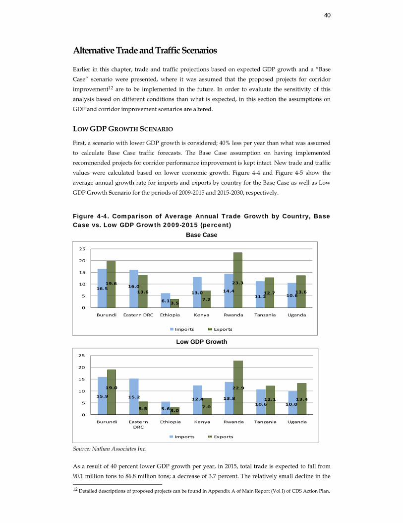
40

16.5 16.0

6.1

13.0 14.411.2 10.6

19.6

13.6

3.57.2

23.3

12.7 13.6

0

5

10

15

20

25

Burundi Eastern DRC Ethiopia Kenya Rwanda Tanzania Uganda

Imports Exports

15.9 15.2

5.6

12.4 13.810.6 10.0

19.0

5.5 3.07.0

22.9

12.1 13.4

0

5

10

15

20

25

Burundi Eastern DRC

Ethiopia Kenya Rwanda Tanzania Uganda

Imports Exports

Alternative Trade and Traffic Scenarios

Earlier in this chapter, trade and traffic projections based on expected GDP growth and a “Base

Case” scenario were presented, where it was assumed that the proposed projects for corridor

improvement12 are to be implemented in the future. In order to evaluate the sensitivity of this analysis based on different conditions than what is expected, in this section the assumptions on

GDP and corridor improvement scenarios are altered.

LOW GDP GROWTH SCENARIO

First, a scenario with lower GDP growth is considered; 40% less per year than what was assumed to calculate Base Case traffic forecasts. The Base Case assumption on having implemented

recommended projects for corridor performance improvement is kept intact. New trade and traffic

values were calculated based on lower economic growth. Figure 4-4 and Figure 4-5 show the average annual growth rate for imports and exports by country for the Base Case as well as Low

GDP Growth Scenario for the periods of 2009-2015 and 2015-2030, respectively.

Figure 4-4. Comparison of Average Annual Trade Growth by Country, Base Case vs. Low GDP Growth 2009-2015 (percent)

Base Case

Low GDP Growth

Source: Nathan Associates Inc.

As a result of 40 percent lower GDP growth per year, in 2015, total trade is expected to fall from 90.1 million tons to 86.8 million tons; a decrease of 3.7 percent. The relatively small decline in the 12 Detailed descriptions of proposed projects can be found in Appendix A of Main Report (Vol I) of CDS Action Plan.

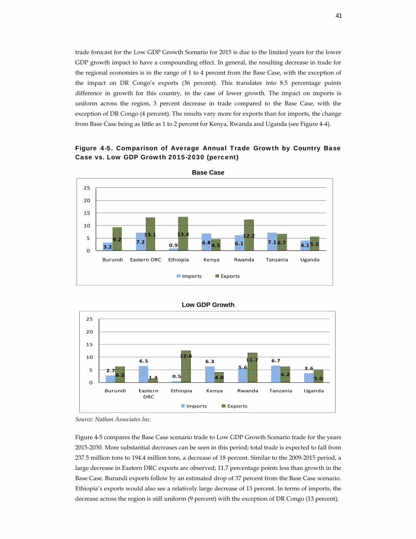
41

3.27.2

0.9 6.8 6.1 7.14.1

9.213.1 13.4

4.5

12.26.7 5.5

0

5

10

15

20

25

Burundi Eastern DRC Ethiopia Kenya Rwanda Tanzania Uganda

Imports Exports

trade forecast for the Low GDP Growth Scenario for 2015 is due to the limited years for the lower

GDP growth impact to have a compounding effect. In general, the resulting decrease in trade for the regional economies is in the range of 1 to 4 percent from the Base Case, with the exception of

the impact on DR Congo’s exports (36 percent). This translates into 8.5 percentage points

difference in growth for this country, in the case of lower growth. The impact on imports is

uniform across the region, 3 percent decrease in trade compared to the Base Case, with the

exception of DR Congo (4 percent). The results vary more for exports than for imports, the change

from Base Case being as little as 1 to 2 percent for Kenya, Rwanda and Uganda (see Figure 4-4).

Figure 4-5. Comparison of Average Annual Trade Growth by Country Base Case vs. Low GDP Growth 2015-2030 (percent)

Base Case

Low GDP Growth

Source: Nathan Associates Inc.

Figure 4-5 compares the Base Case scenario trade to Low GDP Growth Scenario trade for the years

2015-2030. More substantial decreases can be seen in this period; total trade is expected to fall from

237.5 million tons to 194.4 million tons, a decrease of 18 percent. Similar to the 2009-2015 period, a large decrease in Eastern DRC exports are observed; 11.7 percentage points less than growth in the

Base Case. Burundi exports follow by an estimated drop of 37 percent from the Base Case scenario.

Ethiopia’s exports would also see a relatively large decrease of 13 percent. In terms of imports, the decrease across the region is still uniform (9 percent) with the exception of DR Congo (13 percent).

2.7

6.5

0.5

6.35.6

6.7

3.66.2 1.4

12.6

4.0

11.7

6.25.0

0

5

10

15

20

25

Burundi Eastern DRC

Ethiopia Kenya Rwanda Tanzania Uganda

Imports Exports

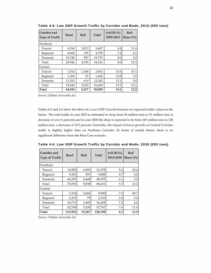
42

Corridor and Type of Traffic

Road Rail TotalAAGR (%) 2009-2015

Rail Share (%)

Transit 6,594 3,013 9,607 8.4 31.4 Regional 4,604 195 4,799 7.4 4.1 Domestic 18,748 987 19,735 8.0 5.0 Total 29,946 4,195 34,141 8.0 12.3

Transit 1,514 1,348 2,862 33.6 47.1 Regional 1,369 55 1,424 12.8 3.9 Domestic 11,763 619 12,382 13.1 5.0 Total 14,646 2,022 16,668 15.3 12.1Total 44,592 6,217 50,809 10.1 12.2

Northern

Central

Corridor and Type of Traffic

Road Rail TotalAAGR (%) 2015-2030

Rail Share (%)

Transit 14,585 6,993 21,578 5.2 32.4 Regional 9,501 397 9,898 4.7 4.0 Domestic 46,507 2,448 48,955 6.1 5.0 Total 70,593 9,838 80,431 5.7 12.2

Transit 5,334 3,666 9,000 7.5 40.7 Regional 2,231 79 2,310 3.0 3.4 Domestic 34,773 1,685 36,458 7.2 4.6 Total 42,338 5,430 47,767 7.0 11.4Total 112,931 15,267 128,198 6.1 11.9

Northern

Central

Table 4-5. Low GDP Growth Traffic by Corridor and Mode, 2015 (000 tons)

Source: Nathan Associates Inc.

Tables 4-5 and 4-6 show the effect of a Low GDP Growth Scenario on expected traffic values in the

future. The total traffic in year 2015 is estimated to drop from 54 million tons to 51 million tons (a

decrease of over 6 percent) and in year 2030 the drop is expected to be from 145 million tons to 128

million tons, a decrease of 10.5 percent. Generally, the impact of lower growth on Central Corridor

traffic is slightly higher than on Northern Corridor. In terms of modal shares, there is no

significant difference from the Base Case scenario.

Table 4-6. Low GDP Growth Traffic by Corridor and Mode, 2030 (000 tons)

Source: Nathan Associates Inc.

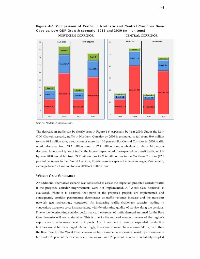
43

Domestic 20.3

Domestic 54.0

Domestic 19.7

Domestic 49.0Transit 11.7

Transit 24.7

Transit 9.6

Transit 21.6

Reg 5.0

Reg 11.0

Reg 4.8

Reg 9.9

‐5

5

15

25

35

45

55

65

75

85

95

2015 2030 2015 2030

BASE CASE LOW GROWTH

Domestic 12.8

Domestic 40.7

Domestic 12.4

Domestic 36.5

Transit 3.2

Transit 12.1

Transit 2.9

Transit 9.0

Reg 1.5

Reg 2.6

Reg 1.4

Reg 2.3

0

10

20

30

40

50

60

2015 2030 2015 2030

BASE CASE LOW GROWTH

Figure 4-6. Comparison of Traffic in Northern and Central Corridors Base Case vs. Low GDP Growth scenario, 2015 and 2030 (million tons)

NORTHERN CORRIDOR CENTRAL CORRIDOR

Source: Nathan Associates Inc.

The decrease in traffic can be clearly seen in Figure 4-6, especially by year 2030: Under the Low

GDP Growth scenario, traffic in Northern Corridor by 2030 is estimated to fall from 89.6 million

tons to 80.4 million tons; a reduction of more than 10 percent. For Central Corridor by 2030, traffic

would decrease from 55.3 million tons to 47.8 million tons, equivalent to about 14 percent

decrease. In terms of types of traffic, the largest impact would be expected on transit traffic, which by year 2030 would fall from 24.7 million tons to 21.6 million tons in the Northern Corridor (12.5

percent decrease). In the Central Corridor, this decrease is expected to be even larger, 25.6 percent,

a change from 12.1 million tons in 2030 to 9 million tons.

WORST CASE SCENARIO

An additional alternative scenario was considered to assess the impact on projected corridor traffic

if the proposed corridor improvements were not implemented. A “Worst Case Scenario” is

evaluated, where it is assumed that none of the proposed projects are implemented and

consequently corridor performance deteriorates as traffic volumes increase and the transport

network gets increasingly congested. As increasing traffic challenges capacity leading to

congestion; transport costs increase along with deteriorating quality of service along the corridor. Due to the deteriorating corridor performance, the forecast of traffic demand assumed for the Base

Case Scenario will not materialize. This is due to the reduced competitiveness of the region’s

exports and the increased cost of imports. Also investment in new or expanded production facilities would be discouraged. Accordingly, this scenario would have a lower GDP growth than

the Base Case. For the Worst Case Scenario we have assumed a worsening corridor performance in

terms of a 25 percent increase in price, time as well as a 25 percent decrease in reliability coupled

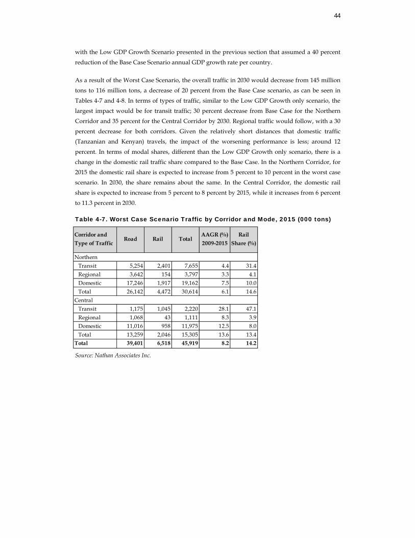
44

Corridor and Type of Traffic

Road Rail TotalAAGR (%) 2009-2015

Rail Share (%)

Transit 5,254 2,401 7,655 4.4 31.4 Regional 3,642 154 3,797 3.3 4.1 Domestic 17,246 1,917 19,162 7.5 10.0 Total 26,142 4,472 30,614 6.1 14.6

Transit 1,175 1,045 2,220 28.1 47.1 Regional 1,068 43 1,111 8.3 3.9 Domestic 11,016 958 11,975 12.5 8.0 Total 13,259 2,046 15,305 13.6 13.4Total 39,401 6,518 45,919 8.2 14.2

Northern

Central

with the Low GDP Growth Scenario presented in the previous section that assumed a 40 percent

reduction of the Base Case Scenario annual GDP growth rate per country.

As a result of the Worst Case Scenario, the overall traffic in 2030 would decrease from 145 million

tons to 116 million tons, a decrease of 20 percent from the Base Case scenario, as can be seen in

Tables 4-7 and 4-8. In terms of types of traffic, similar to the Low GDP Growth only scenario, the

largest impact would be for transit traffic; 30 percent decrease from Base Case for the Northern

Corridor and 35 percent for the Central Corridor by 2030. Regional traffic would follow, with a 30

percent decrease for both corridors. Given the relatively short distances that domestic traffic (Tanzanian and Kenyan) travels, the impact of the worsening performance is less; around 12

percent. In terms of modal shares, different than the Low GDP Growth only scenario, there is a

change in the domestic rail traffic share compared to the Base Case. In the Northern Corridor, for 2015 the domestic rail share is expected to increase from 5 percent to 10 percent in the worst case

scenario. In 2030, the share remains about the same. In the Central Corridor, the domestic rail

share is expected to increase from 5 percent to 8 percent by 2015, while it increases from 6 percent

to 11.3 percent in 2030.

Table 4-7. Worst Case Scenario Traffic by Corridor and Mode, 2015 (000 tons)

Source: Nathan Associates Inc.

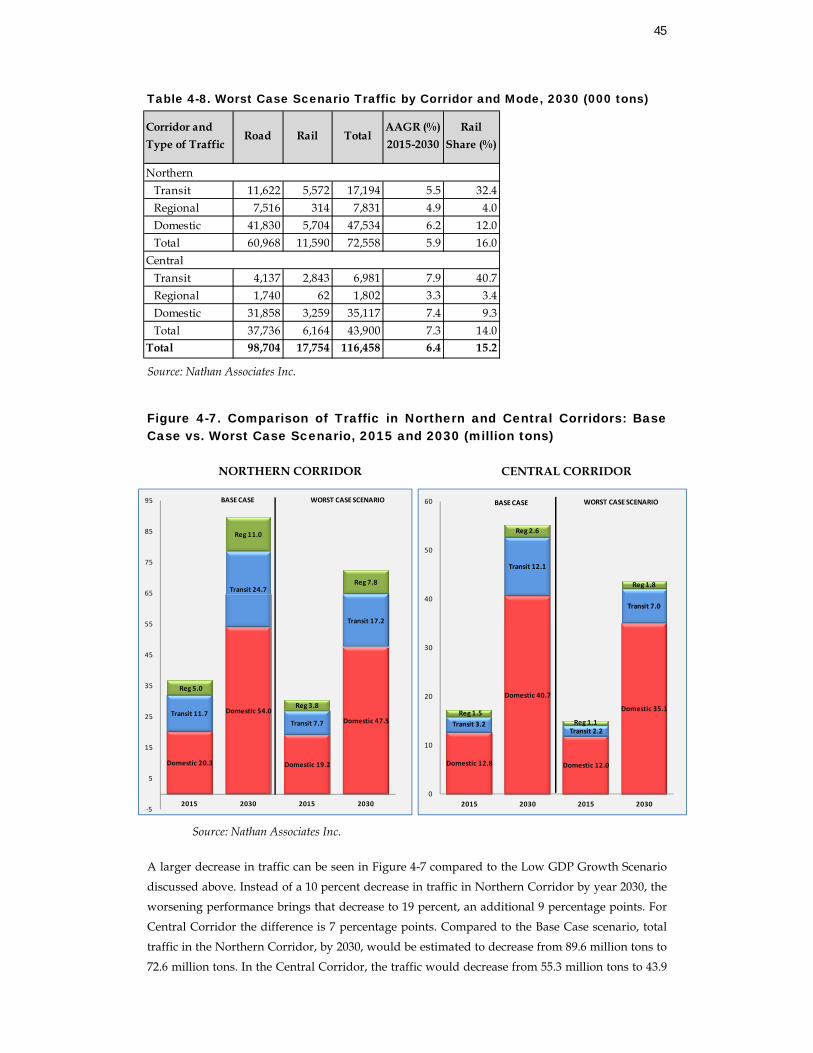
45

Domestic 20.3

Domestic 54.0

Domestic 19.2

Domestic 47.5Transit 11.7

Transit 24.7

Transit 7.7

Transit 17.2

Reg 5.0

Reg 11.0

Reg 3.8

Reg 7.8

‐5

5

15

25

35

45

55

65

75

85

95

2015 2030 2015 2030

BASE CASE WORST CASE SCENARIO

Corridor and Type of Traffic

Road Rail TotalAAGR (%) 2015-2030

Rail Share (%)

Transit 11,622 5,572 17,194 5.5 32.4 Regional 7,516 314 7,831 4.9 4.0 Domestic 41,830 5,704 47,534 6.2 12.0 Total 60,968 11,590 72,558 5.9 16.0

Transit 4,137 2,843 6,981 7.9 40.7 Regional 1,740 62 1,802 3.3 3.4 Domestic 31,858 3,259 35,117 7.4 9.3 Total 37,736 6,164 43,900 7.3 14.0Total 98,704 17,754 116,458 6.4 15.2

Northern

Central

Table 4-8. Worst Case Scenario Traffic by Corridor and Mode, 2030 (000 tons)

Source: Nathan Associates Inc.

Figure 4-7. Comparison of Traffic in Northern and Central Corridors: Base Case vs. Worst Case Scenario, 2015 and 2030 (million tons)

NORTHERN CORRIDOR

Source: Nathan Associates Inc.

A larger decrease in traffic can be seen in Figure 4-7 compared to the Low GDP Growth Scenario

discussed above. Instead of a 10 percent decrease in traffic in Northern Corridor by year 2030, the

worsening performance brings that decrease to 19 percent, an additional 9 percentage points. For

Central Corridor the difference is 7 percentage points. Compared to the Base Case scenario, total

traffic in the Northern Corridor, by 2030, would be estimated to decrease from 89.6 million tons to

72.6 million tons. In the Central Corridor, the traffic would decrease from 55.3 million tons to 43.9

Domestic 12.8

Domestic 40.7

Domestic 12.0

Domestic 35.1

Transit 3.2

Transit 12.1

Transit 2.2

Transit 7.0

Reg 1.5

Reg 2.6

Reg 1.1

Reg 1.8

0

10

20

30

40

50

60

2015 2030 2015 2030

BASE CASE WORST CASE SCENARIO

CENTRAL CORRIDOR

46

million tons. A more significant decrease can be observed in year 2015 in the WCS scenario for

both corridors: For Northern Corridor, the decrease from Base Case values would be about 17 percent and for Central Corridor this value would be 12.5 percent.

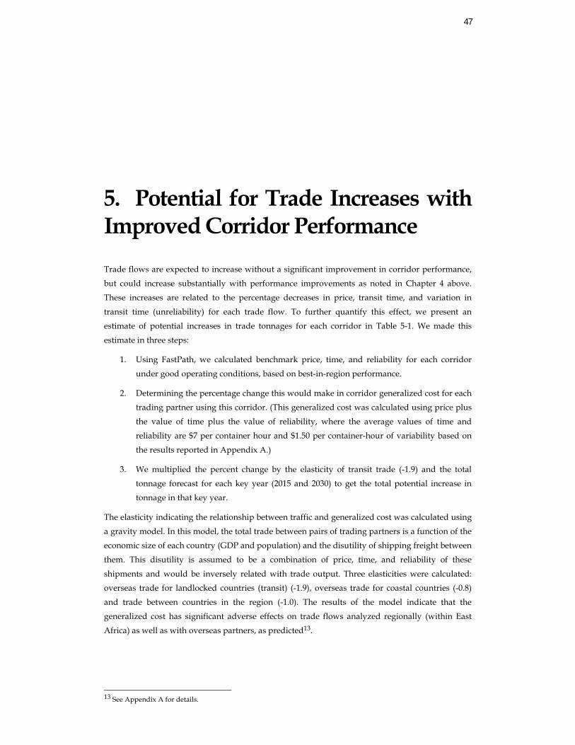
47

5. Potential for Trade Increases with Improved Corridor Performance Trade flows are expected to increase without a significant improvement in corridor performance,

but could increase substantially with performance improvements as noted in Chapter 4 above.

These increases are related to the percentage decreases in price, transit time, and variation in

transit time (unreliability) for each trade flow. To further quantify this effect, we present an

estimate of potential increases in trade tonnages for each corridor in Table 5-1. We made this

estimate in three steps:

1. Using FastPath, we calculated benchmark price, time, and reliability for each corridor

under good operating conditions, based on best-in-region performance.

2. Determining the percentage change this would make in corridor generalized cost for each trading partner using this corridor. (This generalized cost was calculated using price plus

the value of time plus the value of reliability, where the average values of time and

reliability are $7 per container hour and $1.50 per container-hour of variability based on

the results reported in Appendix A.)

3. We multiplied the percent change by the elasticity of transit trade (-1.9) and the total

tonnage forecast for each key year (2015 and 2030) to get the total potential increase in tonnage in that key year.

The elasticity indicating the relationship between traffic and generalized cost was calculated using

a gravity model. In this model, the total trade between pairs of trading partners is a function of the economic size of each country (GDP and population) and the disutility of shipping freight between

them. This disutility is assumed to be a combination of price, time, and reliability of these

shipments and would be inversely related with trade output. Three elasticities were calculated: overseas trade for landlocked countries (transit) (-1.9), overseas trade for coastal countries (-0.8)

and trade between countries in the region (-1.0). The results of the model indicate that the

generalized cost has significant adverse effects on trade flows analyzed regionally (within East

Africa) as well as with overseas partners, as predicted13.

13 See Appendix A for details.

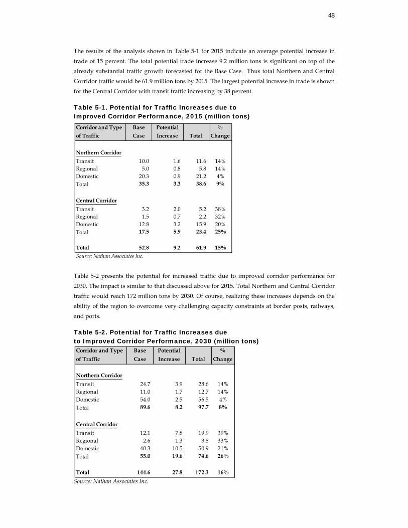
48

Corridor and Type of Traffic

Base Case

Potential Increase Total

% Change

Northern CorridorTransit 10.0 1.6 11.6 14%Regional 5.0 0.8 5.8 14%Domestic 20.3 0.9 21.2 4%Total 35.3 3.3 38.6 9%

Central CorridorTransit 3.2 2.0 5.2 38%Regional 1.5 0.7 2.2 32%Domestic 12.8 3.2 15.9 20%Total 17.5 5.9 23.4 25%

Total 52.8 9.2 61.9 15%Source: Nathan Associates Inc.

Corridor and Type of Traffic

Base Case

Potential Increase Total

% Change

Northern CorridorTransit 24.7 3.9 28.6 14%Regional 11.0 1.7 12.7 14%Domestic 54.0 2.5 56.5 4%Total 89.6 8.2 97.7 8%

Central CorridorTransit 12.1 7.8 19.9 39%Regional 2.6 1.3 3.8 33%Domestic 40.3 10.5 50.9 21%Total 55.0 19.6 74.6 26%

Total 144.6 27.8 172.3 16%

The results of the analysis shown in Table 5-1 for 2015 indicate an average potential increase in

trade of 15 percent. The total potential trade increase 9.2 million tons is significant on top of the already substantial traffic growth forecasted for the Base Case. Thus total Northern and Central

Corridor traffic would be 61.9 million tons by 2015. The largest potential increase in trade is shown

for the Central Corridor with transit traffic increasing by 38 percent.

Table 5-1. Potential for Traffic Increases due to Improved Corridor Performance, 2015 (million tons)

Table 5-2 presents the potential for increased traffic due to improved corridor performance for

2030. The impact is similar to that discussed above for 2015. Total Northern and Central Corridor

traffic would reach 172 million tons by 2030. Of course, realizing these increases depends on the

ability of the region to overcome very challenging capacity constraints at border posts, railways,

and ports.

Table 5-2. Potential for Traffic Increases due to Improved Corridor Performance, 2030 (million tons)

Source: Nathan Associates Inc.

49

This analysis has shown that implementation of the recommended projects will bring major

improvements in the cost, transit time and reliability of the logistic chain of the Northern and Central Corridors. These gains will promote and facilitate trade and economic growth to

significantly contribute to the attainment of the region’s leaders and people development

aspirations.

Appendix A. Technical Description of Transport Models This appendix provides a technical description of the two models which were applied in the

Corridor Diagnostic Study. These models are based on research carried out by Nathan Associates,

Inc. during the Core Network Study.14

Total Trade Model

The total trade between pairs of trading partners is assumed to be a function of the economic size

of the trading partners and inversely related to the disutility of shipping freight between them.

This disutility is assumed to be some combination of price, time, and reliability of these shipments. Other factors may also be significant. To analyze these relationships, we undertook a gravity

modeling exercise to estimate the trade effects of transportation and compared them with

geographic impediments and with trade policy variables. 15

OVERVIEW OF GRAVITY MODEL

For the past 50 years, the basic gravity model has been used to explain aggregate bilateral trade

flows in terms of variables that would attract flows of goods between two economies and variables

that would interfere with that attraction. Size as measured by GDP and population16 is posited as the main attraction while distance has been the standard variable used for trade resistance, but

there are many variations on the basic gravity model. It is common to add other geographic

variables, such as dummy variables for countries sharing a common border, landlocked countries,

island countries, countries sharing a common language, and common institutions (Walley). Policy

variables in gravity models include average tariff rate, nontariff barrier index, openness

indicator,17 and dummy variables for countries with preferential trade arrangements. Measures of

14 More details on these models are presented in the Core Network Study Regional Model Report Appendices C and

D. 15 The term policy variable is used in this chapter in two ways. For gravity modeling, it refers to indicators that

reflect government policy, such as tariff policy, openness of the economy, and trading partners with preferential trade agreements. For corridor choice modeling it is used to indicate corridor choice biases that are influenced by government policies as well as by shipper preferences.

16 Oguledo and MacPhee note that more trade is usually associated with large size but that a large population enables a country to gain from specialization and exchange internally rather than through external trade. Consequently, the sign of the population coefficient may be negative or positive.

17 The Sachs-Warner indicator is a dummy variable that takes zero value if an economy is closed according to any one of the following five criteria: (i) its average tariff rate exceeded 40 percent, (ii) its non-tariff barriers covered more than 40 percent of imports, (iii) it had a socialist economic system (iv) it had a state monopoly of major

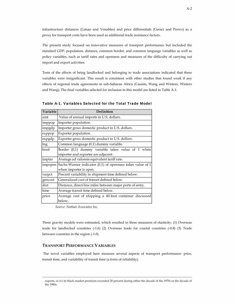
A-2

infrastructure distances (Limao and Venables) and price differentials (Geraci and Prewo) as a

proxy for transport costs have been used as additional trade resistance factors.

The present study focused on innovative measures of transport performance but included the

standard GDP, population, distance, common border, and common language variables as well as

policy variables, such as tariff rates and openness and measures of the difficulty of carrying out

import and export activities.

Tests of the effects of being landlocked and belonging to trade associations indicated that these

variables were insignificant. This result is consistent with other studies that found weak if any

effects of regional trade agreements in sub-Saharan Africa (Cassim, Wang and Winters, Winters

and Wang). The final variables selected for inclusion in this model are listed in Table A-1.

Table A-1. Variables Selected for the Total Trade Model

Source: Nathan Associates Inc.

Three gravity models were estimated, which resulted in three measures of elasticity: (1) Overseas

trade for landlocked countries (-1.6) (2) Overseas trade for coastal countries (-0.8) (3) Trade

between countries in the region (-1.0).

TRANSPORT PERFORMANCE VARIABLES

The novel variables employed here measure several aspects of transport performance: price,

transit time, and variability of transit time (a form of reliability).

exports, or (v) its black-market premium exceeded 20 percent during either the decade of the 1970s or the decade of the 1980s.

Variable Definitionamt Value of annual imports in U.S. dollars.imppop Importer population.impgdp Importer gross domestic product in U.S. dollars.exppop Exporter population.expgdp Exporter gross domestic product in U.S. dollars.lng Common language (0,1) dummy variable.bord Border (0,1) dummy variable takes value of 1 when

importer and exporter are adjacent .imptar Average ad valorem equivalent tariff rate.impopen Sachs-Warner indicator (0,1) of openness takes value of 1

when importer is open.varpct Percent variability in shipment time defined below.gencost Generalized cost of transit defined below.dist Distance, direct-line miles between major ports of entry.time Average transit time defined below.price Average cost of shipping a 40-foot container discussed

below.

A-3

Transport Price

Transport price is defined as the average explicit cost of transporting a standard 40-foot container

between major shipping points, including the cost of export from origin and the cost of import at

destination. Price from coastal countries is calculated as cost of export through the port near the

largest city plus the cost of shipping from that port to the destination country. Price to coastal

countries is calculated as the shipping cost from the origin country plus the import price for the port of the destination country.

Price for imports to landlocked countries from overseas regions is the weighted average of costs

for shipping and for corridor transit (including port import price and land transport) where the weighting is the average percent of historical traffic by corridor and mode (subcorridor). Price for

exports from landlocked countries overseas is the weighted average corridor costs (including port

costs) in the export direction plus overland shipping costs from each corridor port to the destination. In some cases overland transport costs were based on general prices for road or rail

transport in a given year. Where price was not available for the land portion of the corridor in a

given year, the price was interpolated from the data in other years. Rail price indices were also

created for certain countries based on shipper reports (Cook).

Pricing for shipping service is dependent on the shipping service and route, which is more

important than the distance involved. An index for price was constructed from sample data to give the year-by-year variation (Cook).

Transport Time

As noted by Hummels, shipping delays impose inventory-holding costs and depreciation or

spoilage costs that may be magnified if they are incurred at an early stage in the production chain. Moreover, lengthy shipping times may have more severe effects on developing countries such as

those in southern and eastern Africa. Most of these countries are farther from foreign customers or

suppliers. The shipping volumes for these countries are smaller, and so more stops are required to

fill a vessel. Finally, the frequency of ship visits is lower. In the latter case, production times must

be adjusted in accordance with the infrequent ship schedules, and domestic transport must be

coordinated as well to facilitate the export process.

Time elapsed in the transport of goods is measured in hours and includes

• Loading at the origin

• Transfer between modes • Border crossing

• En route activities, such as vehicle weight controls

• Port processing and handling • Customs procedures, and

• Maritime shipping.

Transit time from coastal countries is calculated from shipper reports as time to export through the

port near the largest city plus the shipping time from that port to the destination country. Transit

time to coastal countries is calculated as the shipping time from the origin country plus the import

time through the port of the destination country.

A-4

Transit time for imports to landlocked countries from overseas regions is the weighted average of

time for shipping and for corridor transit (including port import time and land transport time) where the weighting is the average percent of historical traffic by corridor and mode (subcorridor).

Transit time for exports from landlocked countries to overseas destinations is the weighted

average corridor transit time (including port time) in the export direction plus shipping time from

each corridor port to the destination country.

Shipping time is heavily dependent on the frequency and directness of the shipping service

provided to the port used for international freight as well as to the distance to the overseas origin or destination. Ship transit times were assumed to be constant for the ten year period used in the

analysis, as were port transit times, except for Dar-es Salaam where import dwell times by year for

transit traffic were available.

Variability in Transport Time

Premature arrivals or unexpected delays in the receipt of goods also impose costs on importers

that discourage trade. We measure this variability in transport time by calculating the average of

the absolute deviations from the mean transit time to find a measure of variability in hours. This

measure of variability is highly correlated with the mean time, so we divide variability in hours by

the mean time to obtain a percentage measure of variability (varpct). For the coastal countries the

variability is calculated as the time-weighted average of the deviations for both ports and shipping. For the landlocked countries the variability is based on deviations for ports, shipping

and land transportation.

GENERALIZED COST OF TRANSPORT

Price and time have a correlation of 65 percent. To avoid the statistical problems associated with this high covariance, we combined the two transport measures into a compound variable called

generalized cost. The generalized cost is the price as calculated above plus the transit time

multiplied by $9, which is the revealed value of time from a logit model estimated for the region (Cook).

YEARS OF OBSERVATION

Data on variables in the gravity model were collected for the latest ten years available (1999-2008).

This period is sufficiently long to minimize the effects of transient events unrelated to the

economic relationships we are examining. It is also long enough to observe the effects of structural

changes in those relationships. In order to see the influence of particular years, each one (2000-

2008) was entered into preliminary regressions as a dummy variable. The dummies representing years were found to be almost always insignificant, indicating that the regression constant was not

shifting over the period.

GRAVITY MODEL RESULTS

Regression Results

The total trade gravity model regression variables all proved to be highly significant with expected signs. Sizes of both exporters and importers in terms of income and population have a strong

A-5

positive relation with bilateral trade flows. Common language and borders also appear to promote

trade.

In terms of trade policy variables in the truncated world model, it appears that the average tariff

rate performs much better than the Sachs-Warner indicator. However, the significant negative

impact of the tariff rate disappears when percentage variability is added to the regression. In the

regional model, neither variable performed well because there is less variation with respect to

trade policy within the region of southern and eastern Africa.

Turning to the novel transport variables that have been introduced in this gravity model, it

appears that generalized cost has significant expected negative effects on trade flows. This was

true of both the regional and truncated world regressions. The size and significance of the

coefficients suggest that the results are robust.

Implications of Results

The modeling results can be interpreted as elasticities, where the 1.9 elasticity estimate for trade

with respect to generalized cost implies that a 10 percent decrease in generalized cost of transport

is associated with a 19 percent increase in trade. For example, if the generalized cost of $11,377 between neighboring Tanzania and Mozambique in 2008 could be reduced to the $7,203 cost

between neighboring Tanzania and Kenya, the model results suggest that Tanzania-Mozambique

trade could grow 70 percent.

Another comparison of results is possible by focusing on the time variable, a component of the

generalized cost variable. The modeling results show that the elasticity of trade with respect to

time was estimated to be -1.8, when generalized cost is not included. This can be compared with similar elasticity derived from the work of Hummels. According to Hummel’s estimates for the

largest SITC product categories (7 and 8), an average ocean voyage from foreign ports to the U.S.

port of Baltimore lasted 20 days and cost 16 percent of the shipment value. Each day added 0.8 percent to Hummel’s cost, implying an elasticity of negative one, somewhat lower than the time

elasticity of -1.8 in the present study. Hummel did not find any significant time costs for

commodities in SITC 0-6 product categories presumably more important to Africa, and the present

study’s estimate of average transport time is 939 hours or 39 days, almost double Hummel’s

average. This study’s estimate of implicit time cost associated with 939 hours is $8,451(Cook). With

a representative African container shipment value of $60,000, southern and eastern Africa time costs amount to roughly 14 percent of shipment value. Reducing the average African transport

time to the average American time would, according to our elasticity estimate of -1.8, increase

trade by 25 percent.

Corridor and Mode Choice Model

MODEL DESIGN

The corridor choice model was designed to be a generalized logit model that can forecast both corridor choice and mode choice within the chosen corridor at the same time. The choice of

A-6

corridor also implies a choice of port and port country. These choices may be made for

financial/logistics reasons or for policy reasons.

The model assigns traffic to corridor/port combinations and to road or multimodal subcorridors

according to (1) subcorridor performance indicators (logistics price, time and reliability, port ship

service and efficiency of import/export procedures), (2) socioeconomic indicators (language

groupings and economic association groupings), and (3) policy indicators (mode preference for

certain types of traffic and preference for or bias against specific ports or countries). Future

expectations of change in these indicators or changes in policy are predicted and then applied in the model to examine their impact on traffic flow patterns.

The model parameters were derived from statistical analysis of historical data on trade flows by

corridor, estimated measures of corridor performance for each corridor and subcorridor from FastPath analysis, empirical measures of shipping service, import and export efficiency and

implied policy effects. Analyses of the data suggested several submodels that were calibrated

using data from 1999 to 2009.

DATA LIMITATIONS

The model was based on available data sources for traffic flows (historic and current), partial

information on historic data and analysis of corridor performance, readily available data on

economic groupings and language, and newly gathered data on corridor performance.

Unfortunately a complete set of import/export data showing corridor choice by commodity and

tonnage for more than one year was only available for one country (Rwanda) while a wide variety

of data for total tonnage imports and exports for many corridors was available from PMAESA for 1999-200518. There was also a comprehensive report on rail transport and road-rail comparisons

for the East African Community19 covering the years 2000-2006, which gave some detailed

comments on performance data. These were complemented by detailed data collection in 2009 on corridor performance by the study team using the FastPath methodology focusing on price time

and reliability for each link of the transport/logistic corridors and subcorridors.

Additional data was collated from the IMF trade statistics on the value of trade by trading partner, which allowed some analysis of the percentage of trade by trading partner and year between 1999

and 2008. These percentages were applied to trade statistics in tonnages as an approximation of

the direction of trade flows. This was useful for estimating trade flows for modeling purposes, despite the inaccuracies it produces.

CORRIDOR CHOICE MODEL RESULTS

Regression Results

The initial model results lead to the following conclusions for corridor choice in Eastern and

Southern Africa:

18 PMAESA, Facilitation of Transport in Eastern and Southern Africa Transport Corridors, 2006. 19 CPCS, Traffic Working Paper, East African Railways Master Plan Study, East African Community, November

2007.

A-7

1. Transport/logistics performance, shipping service, economic groupings, and policy

choices are all significant factors in corridor choice.

2. Import flows follow a different pattern of corridor, mode, and port choice than export

flows.

3. Northern landlocked countries (Rwanda, Burundi, Uganda, and north eastern DR Congo)

followed a somewhat different pattern than southern landlocked countries (Zambia,

Zimbabwe, and southern DR Congo) due to the wider availability of ports and the

influence of South Africa.

4. Corridor choice for exports is more influenced by policy variables than corridor choice for

imports, which is closely aligned with corridor cost, time, and reliability.

5. The approximation techniques used to fill in data gaps introduced more uncertainty in model results, but the significance of the model coefficients shows that many parts of the

models are robust.

Submodels and Their Variables

The submodels identified for the study are based on the statistical significance of the coefficients of the variables and their overall explanatory power. On the basis of the statistical analysis presented

in Appendix E, there appeared seven submodels:

1. Import corridor choice for Northern Corridor countries

2. Export corridor choice for North-South Corridor countries

3. Import corridor choice for Copper Belt countries

4. Export corridor choice for Copper Belt countries 5. Import and Export corridor choice for Malawi

6. Import and Export corridor choice for Zimbabwe

7. Intraregional corridor choice

The variables used in each submodel are presented in Table A-2 along with comments on the

direction and relative importance of preference or bias indicated by the variables on corridor

choice. The Malawi and Zimbabwe submodels are examples of a more general Southern African

submodel. The relative importance of corridor performance and policy variables (bias and/or

preference for different ports for transshipment and for the use of rail or road modes) in corridor

choice is indicated as well in Table A-2.

Implications of the Submodels

Of the seven submodels, only the two Northern and Central Corridor Import and Export

submodels were able to distinguish the separate influences of price, time and reliability, as there

were a sufficient number of observations to test these relationships. (The other submodels used generalized cost, which combines price and time to avoid the problem of the high covariance

among price, time, and reliability data and lesser number of observations.)

Price to the shippers and transit time are significant in both submodels. Reliability is important only for imports. The bias variable for selection of Dar port vs Mombasa is also significant in both

models. However, it is positive for imports and negative for exports. This variable was significant

even after the performance measures of price, time and reliability were taken into account.

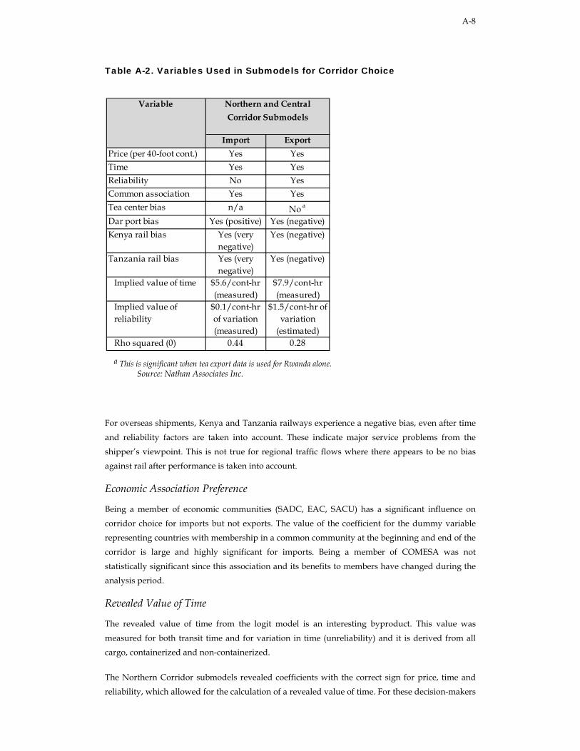
A-8

Table A-2. Variables Used in Submodels for Corridor Choice

a This is significant when tea export data is used for Rwanda alone.

Source: Nathan Associates Inc.

For overseas shipments, Kenya and Tanzania railways experience a negative bias, even after time

and reliability factors are taken into account. These indicate major service problems from the

shipper’s viewpoint. This is not true for regional traffic flows where there appears to be no bias against rail after performance is taken into account.

Economic Association Preference

Being a member of economic communities (SADC, EAC, SACU) has a significant influence on

corridor choice for imports but not exports. The value of the coefficient for the dummy variable

representing countries with membership in a common community at the beginning and end of the

corridor is large and highly significant for imports. Being a member of COMESA was not

statistically significant since this association and its benefits to members have changed during the analysis period.

Revealed Value of Time

The revealed value of time from the logit model is an interesting byproduct. This value was

measured for both transit time and for variation in time (unreliability) and it is derived from all cargo, containerized and non-containerized.

The Northern Corridor submodels revealed coefficients with the correct sign for price, time and

reliability, which allowed for the calculation of a revealed value of time. For these decision-makers

Import Export Price (per 40-foot cont.) Yes YesTime Yes YesReliability No YesCommon association Yes YesTea center bias n/a No a

Dar port bias Yes (positive) Yes (negative)Kenya rail bias Yes (very

negative)Yes (negative)

Tanzania rail bias Yes (very negative)

Yes (negative)

Implied value of time $5.6/cont-hr (measured)

$7.9/cont-hr (measured)

Implied value of reliability

$0.1/cont-hr of variation (measured)

$1.5/cont-hr of variation

(estimated)Rho squared (0) 0.44 0.28

Variable Northern and Central Corridor Submodels

A-9

the value of time is $5.6 to $7.9 per container-hour of transit time (an average of $7), with the

higher value given to Northern Corridor exports (dominated by coffee and tea). Since the longer the time spent on the inland transit routes, the more likely is loss of cargo on that route, this value

probably includes a value of cargo security as well as time.

The value of reliability was calculated at $0.10 per container-hour of variation in transit time for

the import submodel. Although it was not statistically significant in the export submodel due to

the high correlation with transit time and the rail bias variables, it is estimated at $1.50 based on

results from submodels for other corridors and countries in the Eastern and Southern Africa region. This value is in the range of the inventory cost for commodities and reflects the fact that

inventories may have to be increased if there is greater unreliability in transit time. This may be a

logistics consideration for these decision-makers.

Rho Squared Values

Rho squared is an indicator of the model’s ability to explain variance in observed data. These

numbers are artificially depressed due to the nature of the approximation process that introduced

more randomness into the calculations than would be there with more complete information on

routing for different trading partners. For this type of model the rho squared for the Northern

Corridor import submodel is considered very good at explaining variance in corridor choice; it is

considered fair to good for the export submodel. Nonetheless, the significance of the model coefficients in all cases shows that the selected variables will have a reliable influence, even if

understated in their influence on the explanatory power of the model.

TESTS OF CORRIDOR CHOICE MODEL PREDICTIVE ACCURACY

To verify that the submodels were working, we tested to see whether the percentages of freight flows predicted by corridor were comparable to the percentages of total freight flows by corridor

from the base data. A similar test was carried out for subcorridors. We also examined variation in

the percentages for different trading partner pairs to see if the differences were in the right direction, considering corridor performance. Results for the Northern and Central Corridor

submodels are presented in Tables A-3 and A-4. The percentage predictions have some differences

from the actual estimated tonnages, but they are within acceptable ranges.

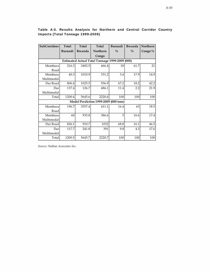
A-10

Table A-3. Results Analysis for Northern and Central Corridor Country Imports (Total Tonnage 1999-2009)

Source: Nathan Associates Inc.

SubCorridors Total Burundi

Total Rwanda

Total Northern

Congo

Burundi %

Rwanda %

Northern Congo %

Mombasa Road

216.3 3482.5 466.4 18 61.7 21

Mombasa Multimodal

40.3 1010.9 331.2 3.4 17.9 14.9

Dar Road 806.4 1025.5 936.9 67.2 18.2 42.2Dar

Multimodal137.4 126.7 486.1 11.4 2.2 21.9

Total 1200.4 5645.6 2220.6 100 100 100

Mombasa Road

196.7 3557.4 411.1 16.4 63 18.5

Mombasa Multimodal

60 935.8 386.6 5 16.6 17.4

Dar Road 826.1 910.7 1032 68.8 16.1 46.5Dar

Multimodal117.7 241.8 391 9.8 4.3 17.6

Total 1200.5 5645.7 2220.7 100 100 100

Estimated Actual Total Tonnage 1999-2009 (000)

Model Prediction 1999-2009 (000 tons)

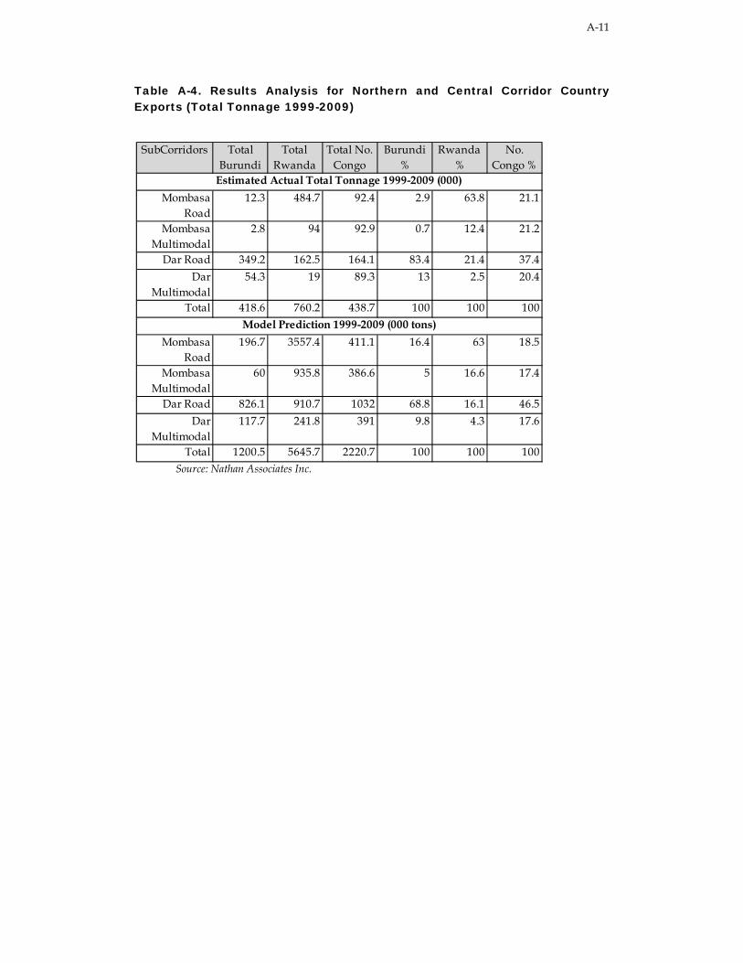
A-11

Table A-4. Results Analysis for Northern and Central Corridor Country Exports (Total Tonnage 1999-2009)

Source: Nathan Associates Inc.

SubCorridors Total Burundi

Total Rwanda

Total No. Congo

Burundi %

Rwanda %

No. Congo %

Mombasa Road

12.3 484.7 92.4 2.9 63.8 21.1

Mombasa Multimodal

2.8 94 92.9 0.7 12.4 21.2

Dar Road 349.2 162.5 164.1 83.4 21.4 37.4Dar

Multimodal54.3 19 89.3 13 2.5 20.4

Total 418.6 760.2 438.7 100 100 100

Mombasa Road

196.7 3557.4 411.1 16.4 63 18.5

Mombasa Multimodal

60 935.8 386.6 5 16.6 17.4

Dar Road 826.1 910.7 1032 68.8 16.1 46.5Dar

Multimodal117.7 241.8 391 9.8 4.3 17.6

Total 1200.5 5645.7 2220.7 100 100 100

Estimated Actual Total Tonnage 1999-2009 (000)

Model Prediction 1999-2009 (000 tons)