metals

Article

Quantitative Assessment of the Time to EndBainitic Transformation

Miguel A. Santajuana 1, Adriana Eres-Castellanos 1 , Victor Ruiz-Jimenez 1, Sebastien Allain 2 ,Guillaume Geandier 2, Francisca G. Caballero 1 and Carlos Garcia-Mateo 1,*

1 Department of Physical Metallurgy, National Center for Metallurgical Research (CENIM-CSIC), AvdaGregorio del Amo, 8, E-28040 Madrid, Spain

2 Institut Jean Lamour, DAMAS Excellence Laboratory, Campus ARTEM, 54000 Nancy, France* Correspondence: cgm@cenim.csic.es; Tel.: +34-91-553-89-00

Received: 5 July 2019; Accepted: 20 August 2019; Published: 23 August 2019�����������������

Abstract: Low temperature bainite consists of an intimate mixture of bainitic ferrite and retainedaustenite, usually obtained by isothermal treatments at temperatures close to the martensite starttemperature and below the bainite start temperature. There is widespread belief regarding theextremely long heat treatments necessary to achieve such a microstructure, but still there are nounified and objective criteria to determine the end of the bainitic transformation that allow formeaningful results and its comparison. A very common way to track such a transformation is bymeans of a high-resolution dilatometer. The relative change in length associated with the bainitictransformation has a very characteristic sigmoidal shape, with low transformation rates at thebeginning and at end of the transformation but rapid in between. The determination of the end oftransformation is normally subjected to the ability and experience of the “operator” and is thereforesubjective. What is more, in the case of very long heat treatments, like those needed for lowtemperature bainite (from hours to days), differences in the criteria used to determine the end oftransformation might lead to differences that might not be assumable from an industrial point ofview. This work reviews some of the most common procedures and attempts to establish a generalcriterion to determine the end of bainitic transformation, based on the differential change in length(transformation rate) derived from a single experiment. The proposed method has been validatedby means of the complementary use of hardness measurements, X-ray diffraction and in situ highenergy X-ray diffraction.

Keywords: bainitic transformation; kinetics; microstructural characterization; incomplete transformation

1. Introduction

Bainite implies a displacive transformation involving a sudden, ordered movement of Fe atoms,also accompanied by a crystal correspondence between the parent austenite and the ferrite lattices, and amacroscopic shape strain of the transformed structure [1]. The process is also known to be diffusionless,and therefore, any excess in C present in a bainitic ferrite plate is partially and immediately releasedto the parent austenite once the plate stops growing [2]. In addition, the precipitation of cementiteprecipitates from the austenite, inherent to the bainitic transformation, can be retarded or even haltedby the use of proper quantities of silicon, i.e., above 1.5 wt.% [3,4]. Thus, finally the microstructure willconsist of partially carbon-supersaturated plates of bainitic ferrite, αb, and C enriched austenite (γ+),the latter as thin films between ferrite plates and submicron blocks between sheaves of bainite [5,6].This microstructure has a high hardness and strength, owing to the combined influence of severaltypes of obstacles to dislocation motion, such as interfaces and dislocations, and also to solid solutionstrengthening and to the interaction between carbon and defects [3,7–17].

Metals 2019, 9, 925; doi:10.3390/met9090925 www.mdpi.com/journal/metals

Metals 2019, 9, 925 2 of 16

A common way to obtain such a microstructure is by intermediate or low temperature isothermaltreatments, above the martensite start temperature (Ms), after full austenitization. In the last decadeor so, such treatments have been successfully applied to Si bearing medium–high C steels (0.5–1wt.%C) in order to obtain the so-called nanostructured bainite [18]. The counterpart in such chemicalcompositions is the fact that transformation at low temperatures can last from few hours to days [19,20].Thus, when envisioning the transfer of this novel metallurgical concept to industrial practices, it isimportant to know and adjust the time of the heat treatments to those strictly necessary—first, becausein that type of time-scales, it can imply an important shorten of the whole process, and second, becauseoverextended treatments can lead to further changes in the microstructure, i.e., autotempering anddecomposition of the bainitic microstructure [21–23].

Through the literature, it is possible to find different methods used to determine the end of thebainite transformation (EBT) [7,24,25], the moment from which there are no more microstructuralchanges. However, as becomes clear through the text, the process of stablishing an EBT is not free fromdifficulties and uncertainties and therefore is not trivial.

In this work, the most common approaches are reviewed, for example, determination of the EBTby interrupted isothermal tests, or graphical and simulation methods based on the dilatometric curvesobtained during the isothermal treatments. Finally, a method is proposed whose solidity lies in the lackof operator decisions (subjectivity) and in the fact that it does not require “ideal” dilatometric curves.

The scientific community can also gain from the establishment of a standardized method of thesecharacteristics, when discussing and comparing the benefits that certain types of actions, such aschemical composition or prior austenite grain size modifications, the effect of plastic deformation, etc.,have in the transformation kinetics of bainite. The described procedure can also be used to get to know,using the dilatometry curve of a single isothermal test, if the bainitic transformation is finished or moretime is required.

2. Materials and Methods

For the purpose of this work, and to take into account any possible differences related to thecarbon content and, in turn, transformation temperatures and kinetics of bainitic transformation, twosteels with different carbon contents were selected. Their chemical compositions are given in Table 1.Steel 1 corresponds to a commercial steel (SCM40), while Steel 2 was developed in the frame of anR & D project [26]. Although their carbon contents are rather different, both of them have a similarbase composition, with differences in the Si content, but in any case sufficient to prevent cementiteformation [3,4].

Table 1. Chemical composition of the steels in wt.%, with Fe to balance, and experimental martensitestart temperature, Ms in ◦C.

Alloy C Si Mn Cr Mo Ni Cu Ms

Steel 1 0.43 3.05 0.71 0.98 0.21 0.09 0.14 280Steel 2 0.99 2.47 0.74 0.98 0.02 0.12 0.19 173Steel 3 0.31 1.52 2.44 320

All heat treatments were performed in a Bahr DIL 805D high-resolution dilatometer usingcylindrical samples 4 mm in diameter and 10 mm in length. During dilatometry measurements, thespecimen is held between two quartz rods, one fixed and the other connected to a LVDT (linear variabledisplacement transducer). Thus, during the whole heat treatment, it was possible to measure therelative change in length (RCL) of the sample. Figure 1a shows the sketch of the isothermal heattreatments performed, where Tγ, TIso and tγ, tIso are the austenitization and isothermal temperaturesand times, respectively. Heating was applied by an induction coil and the temperature controlled by atype K thermocouple spot welded in the center of the specimen. All experiments were carried out invacuum (10−4 mbar). All the heat treatment parameters were carefully selected and adapted to the

Metals 2019, 9, 925 3 of 16

chemical composition of the steels in order to obtain a bainitic structure; the details have been profuselydiscussed in [20,26,27]. Suffice it to say that in order to study the temporal advance of the bainitictransformation, different times tIso were selected, the longest one being enough for the transformationto reach its completion.

Metals 2019, 9, 925 3 of 16

in vacuum (10−4 mbar). All the heat treatment parameters were carefully selected and adapted to the chemical composition of the steels in order to obtain a bainitic structure; the details have been profusely discussed in [20,26,27]. Suffice it to say that in order to study the temporal advance of the bainitic transformation, different times tIso were selected, the longest one being enough for the transformation to reach its completion.

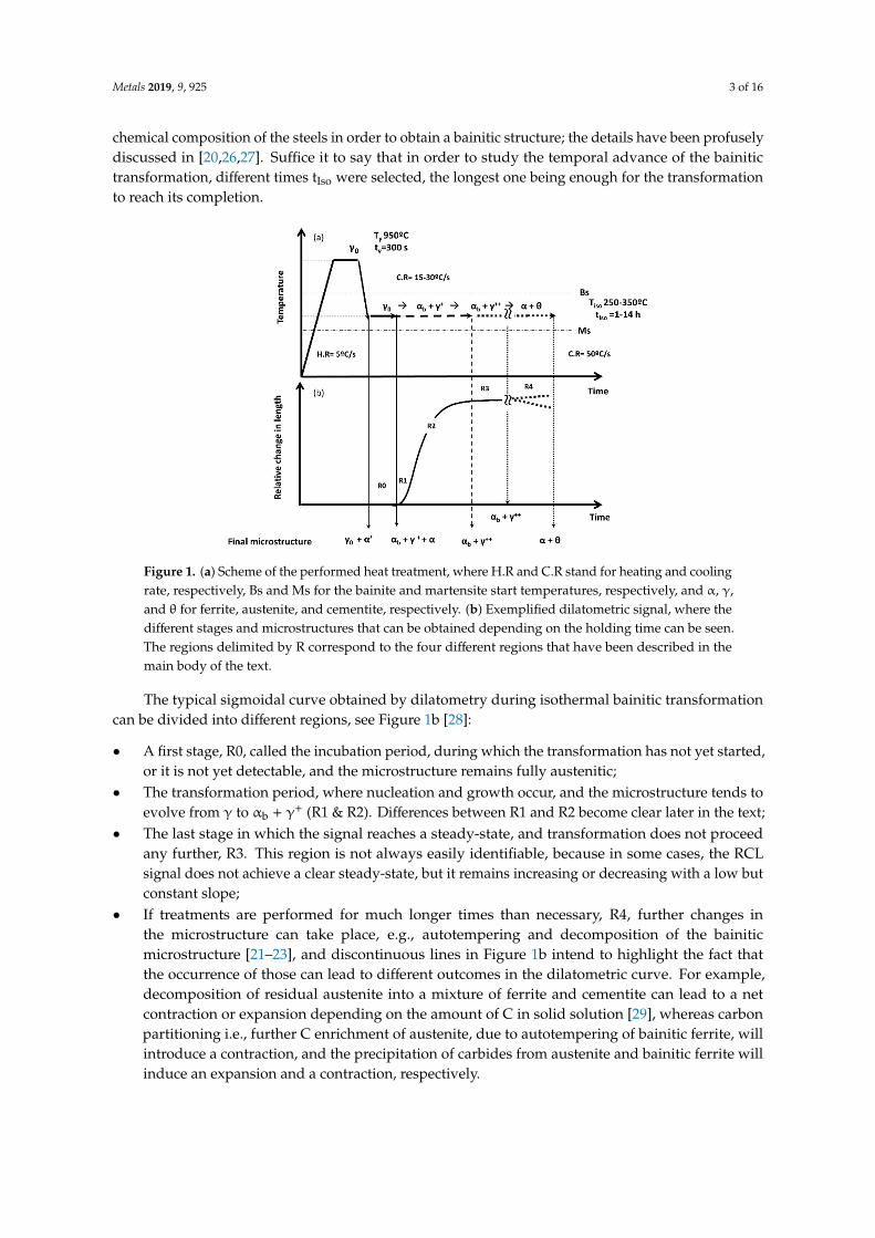
Figure 1. (a) Scheme of the performed heat treatment, where H.R and C.R stand for heating and cooling rate, respectively, Bs and Ms for the bainite and martensite start temperatures, respectively, and α, γ, and θ for ferrite, austenite, and cementite, respectively. (b) Exemplified dilatometric signal, where the different stages and microstructures that can be obtained depending on the holding time can be seen. The regions delimited by R correspond to the four different regions that have been described in the main body of the text.

The typical sigmoidal curve obtained by dilatometry during isothermal bainitic transformation can be divided into different regions, see Figure 1b [28]:

• A first stage, R0, called the incubation period, during which the transformation has not yet started, or it is not yet detectable, and the microstructure remains fully austenitic;

• The transformation period, where nucleation and growth occur, and the microstructure tends to evolve from γ to αb + γ+ (R1 & R2). Differences between R1 and R2 become clear later in the text;

• The last stage in which the signal reaches a steady-state, and transformation does not proceed any further, R3. This region is not always easily identifiable, because in some cases, the RCL signal does not achieve a clear steady-state, but it remains increasing or decreasing with a low but constant slope;

• If treatments are performed for much longer times than necessary, R4, further changes in the microstructure can take place, e.g., autotempering and decomposition of the bainitic microstructure [21–23], and discontinuous lines in Figure 1b intend to highlight the fact that the occurrence of those can lead to different outcomes in the dilatometric curve. For example, decomposition of residual austenite into a mixture of ferrite and cementite can lead to a net contraction or expansion depending on the amount of C in solid solution [29], whereas carbon partitioning i.e., further C enrichment of austenite, due to autotempering of bainitic ferrite, will introduce a contraction, and the precipitation of carbides from austenite and bainitic ferrite will induce an expansion and a contraction, respectively.

Figure 1. (a) Scheme of the performed heat treatment, where H.R and C.R stand for heating and coolingrate, respectively, Bs and Ms for the bainite and martensite start temperatures, respectively, and α, γ,and θ for ferrite, austenite, and cementite, respectively. (b) Exemplified dilatometric signal, where thedifferent stages and microstructures that can be obtained depending on the holding time can be seen.The regions delimited by R correspond to the four different regions that have been described in themain body of the text.

The typical sigmoidal curve obtained by dilatometry during isothermal bainitic transformationcan be divided into different regions, see Figure 1b [28]:

• A first stage, R0, called the incubation period, during which the transformation has not yet started,or it is not yet detectable, and the microstructure remains fully austenitic;

• The transformation period, where nucleation and growth occur, and the microstructure tends toevolve from γ to αb + γ+ (R1 & R2). Differences between R1 and R2 become clear later in the text;

• The last stage in which the signal reaches a steady-state, and transformation does not proceedany further, R3. This region is not always easily identifiable, because in some cases, the RCLsignal does not achieve a clear steady-state, but it remains increasing or decreasing with a low butconstant slope;

• If treatments are performed for much longer times than necessary, R4, further changes inthe microstructure can take place, e.g., autotempering and decomposition of the bainiticmicrostructure [21–23], and discontinuous lines in Figure 1b intend to highlight the fact thatthe occurrence of those can lead to different outcomes in the dilatometric curve. For example,decomposition of residual austenite into a mixture of ferrite and cementite can lead to a netcontraction or expansion depending on the amount of C in solid solution [29], whereas carbonpartitioning i.e., further C enrichment of austenite, due to autotempering of bainitic ferrite, willintroduce a contraction, and the precipitation of carbides from austenite and bainitic ferrite willinduce an expansion and a contraction, respectively.

Metals 2019, 9, 925 4 of 16

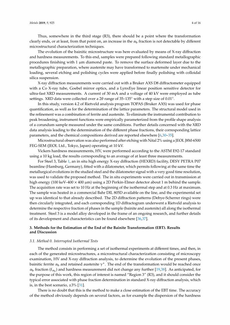
Thus, somewhere in the third stage (R3), there should be a point where the transformationclearly ends, or at least, from that point on, an increase in the αb fraction is not detectable by differentmicrostructural characterization techniques.

The evolution of the bainitic microstructure was here evaluated by means of X-ray diffractionand hardness measurements. To this end, samples were prepared following standard metallographicprocedures finishing with 1 µm diamond paste. To remove the surface deformed layer due to themetallographic preparation, where austenite may have transformed to martensite under mechanicalloading, several etching and polishing cycles were applied before finally polishing with colloidalsilica suspension.

X-ray diffraction measurements were carried out with a Bruker AXS D8 diffractometer equippedwith a Co X-ray tube, Goebel mirror optics, and a LynxEye linear position sensitive detector forultra-fast XRD measurements. A current of 30 mA and a voltage of 40 kV were employed as tubesettings. XRD data were collected over a 2θ range of 35–135◦ with a step size of 0.01◦.

In this study, version 4.2 of Rietveld analysis program TOPAS (Bruker AXS) was used for phasequantification, as well as for the determination of the lattice parameters. The structural model used inthe refinement was a combination of ferrite and austenite. To eliminate the instrumental contribution topeak broadening, instrument functions were empirically parameterized from the profile shape analysisof a corundum sample measured under the same conditions. Further details concerned with the XRDdata analysis leading to the determination of the different phase fractions, their corresponding latticeparameters, and the chemical compositions derived are reported elsewhere [6,30–35].

Microstructural observation was also performed after etching with Nital 2% using a JEOL J8M-6500FEG-SEM (JEOL Ltd., Tokyo, Japan) operating at 10 kV.

Vickers hardness measurements, HV, were performed according to the ASTM E92-17 standardusing a 10 kg load, the results corresponding to an average of at least three measurements.

For Steel 3, Table 1, an in situ high energy X-ray diffraction (HEXRD) facility, DESY PETRA P07beamline (Hamburg, Germany), fitted with a dilatometer, which permits following at the same time themetallurgical evolutions in the studied steel and the dilatometer signal with a very good time resolution,was used to validate the proposed method. The in situ experiments were carried out in transmission athigh energy (100 keV–400 × 400 µm) using a 2D Perkin-Elmer detector about 1 m behind the sample.The acquisition rate was set to 10 Hz at the beginning of the isothermal step and at 0.3 Hz at maximum.The sample was heated in a commercial Bahr DIL 805D available on the line, and the experimental setup was identical to that already described. The 2D diffraction patterns (Debye-Scherrer rings) werethen circularly integrated, and each corresponding 1D diffractogram underwent a Rietveld analysis todetermine the respective fraction of phases in the sample (bainite and austenite) all along the isothermaltreatment. Steel 3 is a model alloy developed in the frame of an ongoing research, and further detailsof its development and characteristics can be found elsewhere [36,37].

3. Methods for the Estimation of the End of the Bainite Transformation (EBT). Resultsand Discussion

3.1. Method 0. Interrupted Isothermal Tests

The method consists in performing a set of isothermal experiments at different times, and then, ineach of the generated microstructures, a microstructural characterization consisting of microscopyexamination, HV and X-ray diffraction analysis, to determine the evolution of the present phases,bainitic ferrite αb and retained austenite γ+. The end of the transformation would be reached onceαb fraction (fαb) and hardness measurement did not change any further [19,38]. As anticipated, forthe purpose of this work, this region of interest is named “Region 3” (R3), and it should consider thetypical error associated with phase fraction determination in standard X-ray diffraction analysis, whichis, in the best scenario, ±3% [31].

There is no doubt that this is the method to make a close estimation of the EBT time. The accuracyof the method obviously depends on several factors, as for example the dispersion of the hardness

Metals 2019, 9, 925 5 of 16

measurements, associated error of XRD experiments, and, finally, number (interval) of interrupted testsperformed to stablish the EBT, beginning of R3. Nevertheless, the method is not without drawbacks,since it requires many samples/materials and consumes a lot of time, not only for the associatedmicrostructural characterization, but also in terms of the time consumed to perform the heat treatments.

Having set the ground for this method, we used it to establish the beginning of the so-calledRegion 3, dotted lines delimiting it in Figures 2 and 3, and to determine if other methods providereliable results, i.e., EBT times within this region.

Figures 2 and 3 gather the results obtained for Steel 1 and Steel 2, respectively, in terms offerritic phase (fα) fraction and hardness of the microstructure. The plots also include the relativechange in length (RCL) signal of the longest test performed, and also indicated are the positions of theinterrupted tests.

In those same figures, the mentioned regions are delimited, but attending to the microstructureobtained after cooling to room temperature, see also Figure 1b.

Metals 2019, 9, 925 5 of 16

There is no doubt that this is the method to make a close estimation of the EBT time. The accuracy of the method obviously depends on several factors, as for example the dispersion of the hardness measurements, associated error of XRD experiments, and, finally, number (interval) of interrupted tests performed to stablish the EBT, beginning of R3. Nevertheless, the method is not without drawbacks, since it requires many samples/materials and consumes a lot of time, not only for the associated microstructural characterization, but also in terms of the time consumed to perform the heat treatments.

Having set the ground for this method, we used it to establish the beginning of the so-called Region 3, dotted lines delimiting it in Figures 2 and 3, and to determine if other methods provide reliable results, i.e., EBT times within this region.

Figures 2 and 3 gather the results obtained for Steel 1 and Steel 2, respectively, in terms of ferritic phase (f ) fraction and hardness of the microstructure. The plots also include the relative change in length (RCL) signal of the longest test performed, and also indicated are the positions of the interrupted tests.

Figure 2. For Steel 1 treated at different isothermal temperatures and times, (a) experimental fraction of ferrite (f ) and Vickers hardness measurements (HV) as a function of time, (b) the relative change in length (RCL) from the dilatometry test, and (c) normalized derivative of the relative change in length (DRCL). The x symbols in (b,c) indicate the position of the interrupted tests whose f and HV are also indicated in (a). Vertical dotted lines denote the limits of regions (R1 and R3) as described in the main body of the text and schematically shown in Figure 1. Note that region R2 is not detectable for Steel 1.

Figure 2. For Steel 1 treated at different isothermal temperatures and times, (a) experimental fraction offerrite (fα) and Vickers hardness measurements (HV) as a function of time, (b) the relative change inlength (RCL) from the dilatometry test, and (c) normalized derivative of the relative change in length(DRCL). The x symbols in (b,c) indicate the position of the interrupted tests whose fα and HV are alsoindicated in (a). Vertical dotted lines denote the limits of regions (R1 and R3) as described in the mainbody of the text and schematically shown in Figure 1. Note that region R2 is not detectable for Steel 1.

Metals 2019, 9, 925 6 of 16Metals 2019, 9, 925 6 of 16

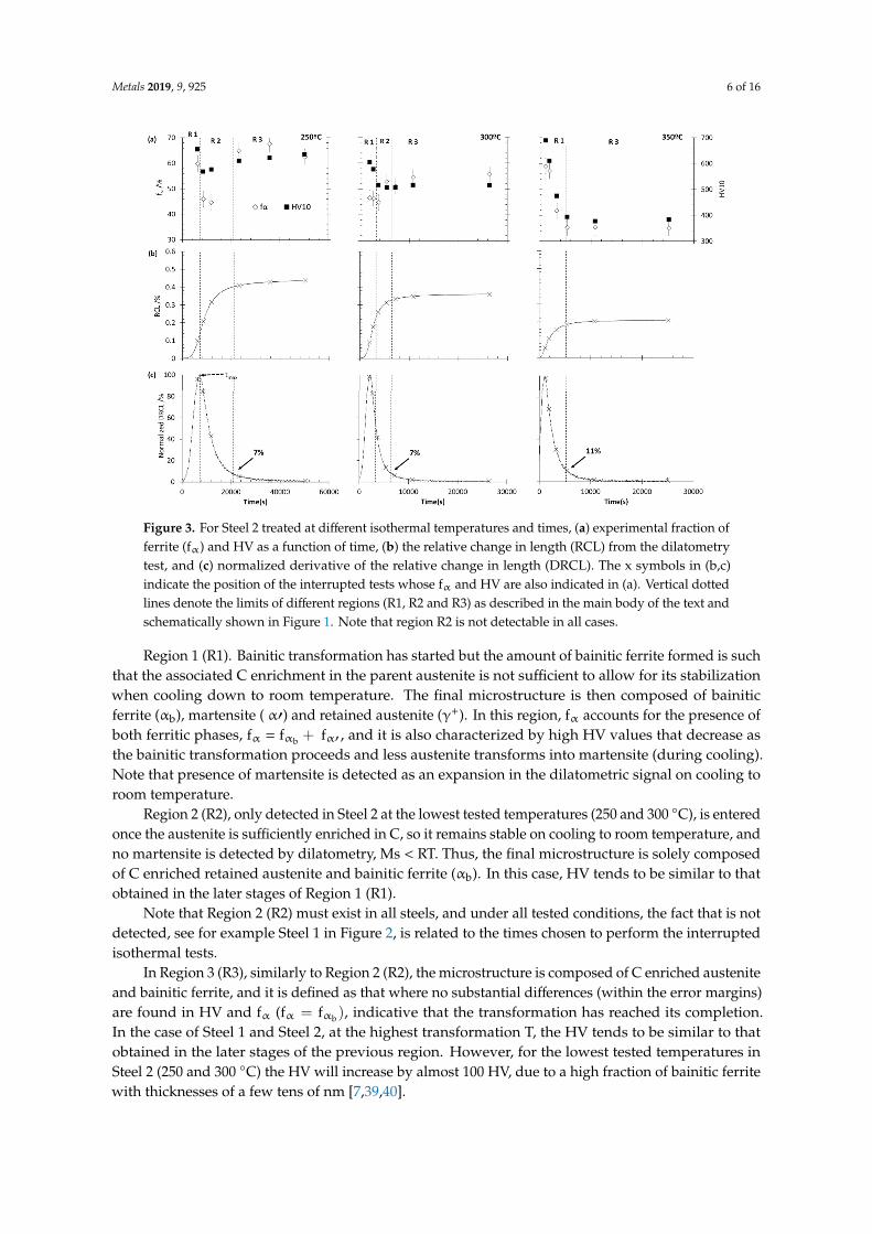
Figure 3. For Steel 2 treated at different isothermal temperatures and times, (a) experimental fraction of ferrite (f ) and HV as a function of time, (b) the relative change in length (RCL) from the dilatometry test, and (c) normalized derivative of the relative change in length (DRCL). The x symbols in (b,c) indicate the position of the interrupted tests whose f and HV are also indicated in (a). Vertical dotted lines denote the limits of different regions (R1, R2 and R3) as described in the main body of the text and schematically shown in Figure 1. Note that region R2 is not detectable in all cases.

In those same figures, the mentioned regions are delimited, but attending to the microstructure obtained after cooling to room temperature, see also Figure 1b.

Region 1 (R1). Bainitic transformation has started but the amount of bainitic ferrite formed is such that the associated C enrichment in the parent austenite is not sufficient to allow for its stabilization when cooling down to room temperature. The final microstructure is then composed of bainitic ferrite (α ), martensite (α ) and retained austenite (γ+). In this region, f accounts for the presence of both ferritic phases, f = f + f , and it is also characterized by high HV values that decrease as the bainitic transformation proceeds and less austenite transforms into martensite (during cooling). Note that presence of martensite is detected as an expansion in the dilatometric signal on cooling to room temperature.

Region 2 (R2), only detected in Steel 2 at the lowest tested temperatures (250 and 300 °C), is entered once the austenite is sufficiently enriched in C, so it remains stable on cooling to room temperature, and no martensite is detected by dilatometry, Ms < RT. Thus, the final microstructure is solely composed of C enriched retained austenite and bainitic ferrite (α ). In this case, HV tends to be similar to that obtained in the later stages of Region 1 (R1).

Note that Region 2 (R2) must exist in all steels, and under all tested conditions, the fact that is not detected, see for example Steel 1 in Figure 2, is related to the times chosen to perform the interrupted isothermal tests.

In Region 3 (R3), similarly to Region 2 (R2), the microstructure is composed of C enriched austenite and bainitic ferrite, and it is defined as that where no substantial differences (within the error margins) are found in HV and f (f = f ), indicative that the transformation has reached its completion. In the case of Steel 1 and Steel 2, at the highest transformation T, the HV tends to be similar to that obtained in the later stages of the previous region. However, for the lowest tested

Figure 3. For Steel 2 treated at different isothermal temperatures and times, (a) experimental fraction offerrite (fα) and HV as a function of time, (b) the relative change in length (RCL) from the dilatometrytest, and (c) normalized derivative of the relative change in length (DRCL). The x symbols in (b,c)indicate the position of the interrupted tests whose fα and HV are also indicated in (a). Vertical dottedlines denote the limits of different regions (R1, R2 and R3) as described in the main body of the text andschematically shown in Figure 1. Note that region R2 is not detectable in all cases.

Region 1 (R1). Bainitic transformation has started but the amount of bainitic ferrite formed is suchthat the associated C enrichment in the parent austenite is not sufficient to allow for its stabilizationwhen cooling down to room temperature. The final microstructure is then composed of bainiticferrite (αb), martensite ( α′) and retained austenite (γ+). In this region, fα accounts for the presence ofboth ferritic phases, fα = fαb + fα′ , and it is also characterized by high HV values that decrease asthe bainitic transformation proceeds and less austenite transforms into martensite (during cooling).Note that presence of martensite is detected as an expansion in the dilatometric signal on cooling toroom temperature.

Region 2 (R2), only detected in Steel 2 at the lowest tested temperatures (250 and 300 ◦C), is enteredonce the austenite is sufficiently enriched in C, so it remains stable on cooling to room temperature, andno martensite is detected by dilatometry, Ms < RT. Thus, the final microstructure is solely composedof C enriched retained austenite and bainitic ferrite (αb). In this case, HV tends to be similar to thatobtained in the later stages of Region 1 (R1).

Note that Region 2 (R2) must exist in all steels, and under all tested conditions, the fact that is notdetected, see for example Steel 1 in Figure 2, is related to the times chosen to perform the interruptedisothermal tests.

In Region 3 (R3), similarly to Region 2 (R2), the microstructure is composed of C enriched austeniteand bainitic ferrite, and it is defined as that where no substantial differences (within the error margins)are found in HV and fα (fα = fαb), indicative that the transformation has reached its completion.In the case of Steel 1 and Steel 2, at the highest transformation T, the HV tends to be similar to thatobtained in the later stages of the previous region. However, for the lowest tested temperatures inSteel 2 (250 and 300 ◦C) the HV will increase by almost 100 HV, due to a high fraction of bainitic ferritewith thicknesses of a few tens of nm [7,39,40].

Metals 2019, 9, 925 7 of 16

Examples of the microstructure obtained in that region after isothermal transformation at 300 ◦Care shown for Steel 1 and Steel 2 in Figure 4a,b, respectively, where the darker long slender features arethe plates of bainitic ferrite (αb), and the lighter phase found as films and more blocky type featurescorrespond to retained austenite (γ).

Metals 2019, 9, 925 7 of 16

temperatures in Steel 2 (250 and 300 °C) the HV will increase by almost 100 HV, due to a high fraction of bainitic ferrite with thicknesses of a few tens of nm [7,39,40].

Examples of the microstructure obtained in that region after isothermal transformation at 300 °C are shown for Steel 1 and Steel 2 in Figure 4a,b, respectively, where the darker long slender features are the plates of bainitic ferrite (α ), and the lighter phase found as films and more blocky type features correspond to retained austenite (γ).

Figure 4. SEM images of the bainitic microstructure obtained after isothermal transformation at 300 °C in (a) Steel 1 and (b) Steel 2. The darker long slender features are the plates of bainitic ferrite (α ), and the lighter phase found as films and more blocky type features correspond to retained austenite (γ).

3.2. Method I. Graphical Method

This method, due to its simplicity, tends to be one of the most widespread. Based on the RCL dilatometric curve obtained during the isothermal treatment, a horizontal line is drawn on the “plateau” (Region 3), and the point at which they both separate is then designated as the EBT time [41–43], see the 1st case in Figure 5. This method strongly depends on the dilatometry signal reaching a total horizontality in Region 3, which does not always happen. In this sense, Figure 5 shows the same experiment as that in the 1st case but leading to a very different scenario, the 2nd case, where the curve, after following the same trend as in the 1st case, and once it has reached the maximum, slowly decreases. Note that the presented data have not been smoothed or filtered and therefore correspond to the actual experiments, but, in any case, the microstructural characterization at the end of both tests lead to almost identical results, with HV of 508 ± 3 and 502 ± 1 and f of 79% and 80%, respectively. Steel 1 at 325 °C in Figure 2b shows a similar, although less accentuated, decrease in RCL. Nor is it strange to find cases where the dilatometry curve seems to slowly and continuously increase in Region 3, see, for example, Steel 2 at 250 °C in Figure 3b, with no apparent microstructural changes taking place, see results in Figure 3a. Some of the technical explanations for such behaviors are found in the fact that there is an inherent dilatometer drift, associated with the thermal interaction at the contact point between the pushrod and the sample, especially during long isothermal treatments.

These being the main drawbacks of the method, we must also consider a subjectivity factor when deciding where and how to draw the horizontal line as well as the determination of the intersection with the dilatometric curve.

Figure 4. SEM images of the bainitic microstructure obtained after isothermal transformation at 300 ◦Cin (a) Steel 1 and (b) Steel 2. The darker long slender features are the plates of bainitic ferrite (αb), andthe lighter phase found as films and more blocky type features correspond to retained austenite (γ).

3.2. Method I. Graphical Method

This method, due to its simplicity, tends to be one of the most widespread. Based on the RCLdilatometric curve obtained during the isothermal treatment, a horizontal line is drawn on the “plateau”(Region 3), and the point at which they both separate is then designated as the EBT time [41–43], seethe 1st case in Figure 5. This method strongly depends on the dilatometry signal reaching a totalhorizontality in Region 3, which does not always happen. In this sense, Figure 5 shows the sameexperiment as that in the 1st case but leading to a very different scenario, the 2nd case, where thecurve, after following the same trend as in the 1st case, and once it has reached the maximum, slowlydecreases. Note that the presented data have not been smoothed or filtered and therefore correspondto the actual experiments, but, in any case, the microstructural characterization at the end of both testslead to almost identical results, with HV of 508 ± 3 and 502 ± 1 and fαb of 79% and 80%, respectively.Steel 1 at 325 ◦C in Figure 2b shows a similar, although less accentuated, decrease in RCL. Nor is itstrange to find cases where the dilatometry curve seems to slowly and continuously increase in Region3, see, for example, Steel 2 at 250 ◦C in Figure 3b, with no apparent microstructural changes takingplace, see results in Figure 3a. Some of the technical explanations for such behaviors are found in thefact that there is an inherent dilatometer drift, associated with the thermal interaction at the contactpoint between the pushrod and the sample, especially during long isothermal treatments.Metals 2019, 9, 925 8 of 16

Figure 5. For Steel 1 treated at 350 °C, the relative change in length of two identical test leading to different dilatometric curves. Also marked is the end of the bainite transformation (EBT) obtained by means of Method I.

3.3. Method II. Dilatometric Curve Simulation by Atomic Volumes

In this method, a combination of some experimental data, dilatometry of the longest experiment in Region 3 and its XRD analysis, together with atomic volume calculations, are used in an attempt to simulate the RCL curve and, in turn, the f vs. time, from where an estimation of the EBT can be made [44–46]. The principles of the method are as follows.

At constant temperature, any change in the RCL curve must be associated with a phase transformation. The density change resulting from the appearance of a new phase, with a different lattice parameter and unit cell, leads to a change in the total length of the sample. Considering bainitic transformation as isotropic, it is possible to calculate the dilatation associated to the transformation based on atomic volumes. Under such an assumption, the relative change in volume (∆V/V ) is related to the relative change in length (∆L/L ) as follows: ∆VV = V − VV = (L + ∆L) − LL ≅ 3 ∆LL (1)

where L and V stand for the length and volume of the sample and the subscript 0 and f for initial and final state, respectively.

The term ∆L/L is directly obtained from dilatometry curves, while the term ∆V/V can be obtained through the specific volumes and the amount of the different phases in the microstructure for the initial and final state. In this way, the initial and final volume for the bainite transformation can be obtained using the following expressions: V = f V + f V (2) V = f V (3)

where fi is the fraction and V is the specific volume of the corresponding phases, i.e., initial austenite (γ), bainitic ferrite (α ), and C enriched retained austenite (γ ). The corresponding atomic volumes ( V , V , and V ), can be calculated from the different lattice parameters obtained from XRD experiments, see Table 2, following the expressions shown in Table 3 [33,47]. The fractions f and f are those also obtained by XRD, while f = 100%, as bainitic ferrite will start to form from a fully austenitic microstructure. It is necessary to remark that in the context of low temperature bainite, the carbon that persists in solid solution within the bainitic ferrite, even after extended heat treatments, is sufficiently Zener ordered to cause the bainitic ferrite unit cell to be noncubic but tetragonal [30,48–50].

Figure 5. For Steel 1 treated at 350 ◦C, the relative change in length of two identical test leading todifferent dilatometric curves. Also marked is the end of the bainite transformation (EBT) obtained bymeans of Method I.

Metals 2019, 9, 925 8 of 16

These being the main drawbacks of the method, we must also consider a subjectivity factor whendeciding where and how to draw the horizontal line as well as the determination of the intersectionwith the dilatometric curve.

3.3. Method II. Dilatometric Curve Simulation by Atomic Volumes

In this method, a combination of some experimental data, dilatometry of the longest experimentin Region 3 and its XRD analysis, together with atomic volume calculations, are used in an attempt tosimulate the RCL curve and, in turn, the fαb vs. time, from where an estimation of the EBT can bemade [44–46]. The principles of the method are as follows.

At constant temperature, any change in the RCL curve must be associated with a phasetransformation. The density change resulting from the appearance of a new phase, with a differentlattice parameter and unit cell, leads to a change in the total length of the sample. Considering bainitictransformation as isotropic, it is possible to calculate the dilatation associated to the transformationbased on atomic volumes. Under such an assumption, the relative change in volume (∆V/V0) isrelated to the relative change in length (∆L/L0) as follows:

∆VV0

=Vf −V0

V0=

(L0 + ∆L)3− L3

0

L30

� 3∆LL0

(1)

where L and V stand for the length and volume of the sample and the subscript 0 and f for initial andfinal state, respectively.

The term ∆L/L0 is directly obtained from dilatometry curves, while the term ∆V/V0 can beobtained through the specific volumes and the amount of the different phases in the microstructure forthe initial and final state. In this way, the initial and final volume for the bainite transformation can beobtained using the following expressions:

Vf = fγ+Vγ+ + fαb Vαb (2)

V0 = fγVγ (3)

where fi is the fraction and Vi is the specific volume of the corresponding phases, i.e., initial austenite(γ), bainitic ferrite (αb), and C enriched retained austenite (γ+). The corresponding atomic volumes(Vγ+ , Vα, and Vγ), can be calculated from the different lattice parameters obtained from XRDexperiments, see Table 2, following the expressions shown in Table 3 [33,47]. The fractions fγ+ and fαb

are those also obtained by XRD, while fγ = 100%, as bainitic ferrite will start to form from a fullyaustenitic microstructure. It is necessary to remark that in the context of low temperature bainite, thecarbon that persists in solid solution within the bainitic ferrite, even after extended heat treatments, issufficiently Zener ordered to cause the bainitic ferrite unit cell to be noncubic but tetragonal [30,48–50].

Table 2. Lattice parameters for austenite (aγ) and bainitic ferrite (aα and cα) obtained fromXRD experiments.

Alloy TIso/◦C aγ/Å aα/Å cα/Å

Steel 1300 3.612 2.852 2.876325 3.614 2.853 2.875350 3.609 2.854 2.877

Steel 2250 3.627 2.852 2.877300 3.626 2.850 2.876350 3.621 2.854 2.874

Metals 2019, 9, 925 9 of 16

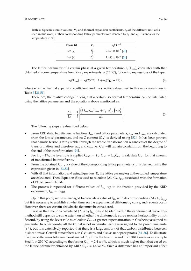
Table 3. Specific atomic volume, Vi, and thermal expansion coefficients, ei, of the different unit cellsused in this work, i. Their corresponding lattice parameters are denoted by ai, and ci. T stands for thetemperature in ◦C.

Phase (i) Vi ei/◦C−1

fcc (γ) a3i

42.065 × 10−5 [21]

bct (a) a2i c2

1.490 × 10−5 [51]

The lattice parameter of a certain phase at a given temperature, ai(TIso), correlates with thatobtained at room temperature from X-ray experiments, ai(25 ◦C), following expressions of the type:

ai(TIso) = ai(25 ◦C)(1 + ei(TIso − 25)), (4)

where ei is the thermal expansion coefficient, and the specific values used in this work are shown inTable 3 [21,51].

Therefore, the relative change in length at a certain isothermal temperature can be calculatedusing the lattice parameters and the equations above mentioned as:

∆LL0

=13

(2 fαb aαb

2cαb + fγ+a3γ+

)− a3

γ

a3γ

. (5)

The following steps are described below:

• From XRD data, bainitic ferrite fraction (fαb) and lattice parameters, aαb and cαb , are calculatedfrom the lattice parameters, and its C content (Cα) is derived using [52]. It has been proventhat bainitic ferrite is fairly stable through the whole transformation regardless of the degree oftransformation, and therefore, aαb and cαb , i.e., Cα, will remain constant from the beginning tothe end of the transformation [24].

• For fαb = 1%, the lever rule is applied Cbulk = fγ+Cγ+ + fαb Cαb to calculate Cγ+ for that amountof transformed bainitic ferrite.

• From the obtained Cγ+ , a value of the corresponding lattice parameter aγ+ is derived using the

expression given in [33,53].• With all that information, and using Equation (4), the lattice parameters at the studied temperature

are calculated. Then, Equation (5) is used to calculate (∆L/L0 )1%, associated with the formationof 1% of bainitic ferrite.

• The process is repeated for different values of fαb up to the fraction provided by the XRDexperiment, fαb = fXRD .

Up to this point, we have managed to correlate a value of fαb with its corresponding (∆L/L0 )fαb,

but it is necessary to establish at what time, on the experimental dilatometry curve, such events occur.However, there are certain drawbacks that must be considered.

First, as the time for a calculated (∆L/L0 )fαbhas to be identified in the experimental curve, this

method still depends to some extent on whether the dilatometric curve reaches horizontality or not.Second, by using the lever rule to calculate Cγ+ , a greater supersaturation in C is being assigned toaustenite. In other words, all the C that is not in bainitic ferrite is assigned to the parent austenite(γ+), but it is extensively reported that there is a large amount of that carbon distributed betweendislocations as Cottrell atmospheres, in C clusters, and also as nanoprecipitates [54–56]. To illustratethe great differences between the estimated Cγ+ from the lever rule and from XRD, serve as an exampleSteel 1 at 250 ◦C, according to the former Cγ+ = 2.4 wt.%, which is much higher than that based onthe lattice parameter obtained by XRD, Cγ+ = 1.4 wt.%. Such a difference has an important effect

Metals 2019, 9, 925 10 of 16

in the (∆L/L0 )fαbcalculations as they rely on estimated lattice parameters. Finally, the theoretical

calculations take into account neither the influence of dislocation density, introduced during thetransformation [45], nor the internal stresses introduced during cooling to room temperature in themicrostructure, as a consequence of the different thermal expansion coefficients of austenite and bainiticferrite [37].

For all those reasons, normalization, to the maximum of the experimental and calculated (∆L/L0)

curves, has proven to minimize such disagreements. Therefore:

• The newly obtained results are then normalized, as it is also the experimental (∆L/L0 ) curve.• From the normalized (∆L/L0 )fαb

, a match is found in the—also normalized—dilatometric curve,and therefore, its corresponding experimental time is established.

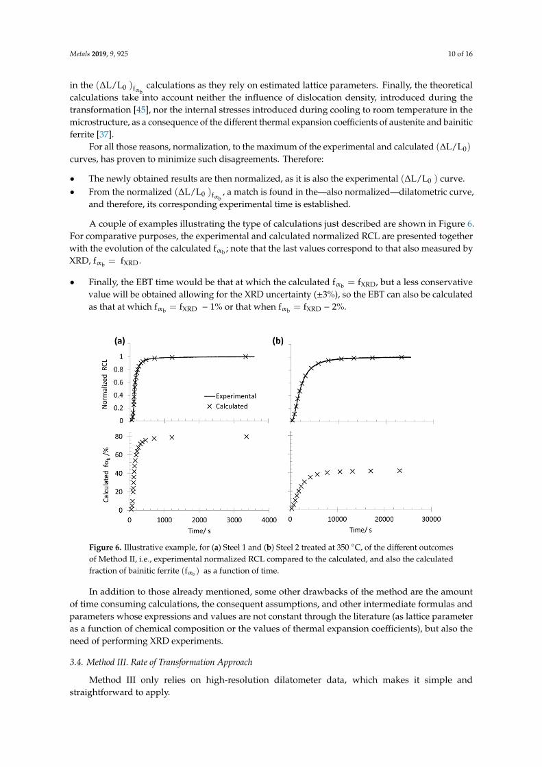
A couple of examples illustrating the type of calculations just described are shown in Figure 6.For comparative purposes, the experimental and calculated normalized RCL are presented togetherwith the evolution of the calculated fαb ; note that the last values correspond to that also measured byXRD, fαb = fXRD .

• Finally, the EBT time would be that at which the calculated fαb = fXRD, but a less conservativevalue will be obtained allowing for the XRD uncertainty (±3%), so the EBT can also be calculatedas that at which fαb = fXRD − 1% or that when fαb = fXRD − 2%.

Metals 2019, 9, 925 10 of 16

First, as the time for a calculated (∆L/L ) has to be identified in the experimental curve, this method still depends to some extent on whether the dilatometric curve reaches horizontality or not. Second, by using the lever rule to calculate C , a greater supersaturation in C is being assigned to austenite. In other words, all the C that is not in bainitic ferrite is assigned to the parent austenite (γ ), but it is extensively reported that there is a large amount of that carbon distributed between dislocations as Cottrell atmospheres, in C clusters, and also as nanoprecipitates [54–56]. To illustrate the great differences between the estimated C from the lever rule and from XRD, serve as an example Steel 1 at 250 °C, according to the former C = 2.4 wt.%, which is much higher than that based on the lattice parameter obtained by XRD, C = 1.4 wt.%. Such a difference has an important effect in the (∆L/L ) calculations as they rely on estimated lattice parameters. Finally, the theoretical calculations take into account neither the influence of dislocation density, introduced during the transformation [45], nor the internal stresses introduced during cooling to room temperature in the microstructure, as a consequence of the different thermal expansion coefficients of austenite and bainitic ferrite [37].

For all those reasons, normalization, to the maximum of the experimental and calculated (∆L/L ) curves, has proven to minimize such disagreements. Therefore:

• The newly obtained results are then normalized, as it is also the experimental (∆L/L ) curve. • From the normalized (∆L/L ) , a match is found in the—also normalized—dilatometric curve,

and therefore, its corresponding experimental time is established.

A couple of examples illustrating the type of calculations just described are shown in Figure 6. For comparative purposes, the experimental and calculated normalized RCL are presented together with the evolution of the calculated f ; note that the last values correspond to that also measured by XRD, f = f .

• Finally, the EBT time would be that at which the calculated f = f , but a less conservative value will be obtained allowing for the XRD uncertainty (±3%), so the EBT can also be calculated as that at which f = f − 1% or that when f = f − 2%.

In addition to those already mentioned, some other drawbacks of the method are the amount of time consuming calculations, the consequent assumptions, and other intermediate formulas and parameters whose expressions and values are not constant through the literature (as lattice parameter as a function of chemical composition or the values of thermal expansion coefficients), but also the need of performing XRD experiments.

Figure 6. Illustrative example, for (a) Steel 1 and (b) Steel 2 treated at 350 °C, of the different outcomes of Method II, i.e., experimental normalized RCL compared to the calculated, and also the calculated fraction of bainitic ferrite (f ) as a function of time.

Figure 6. Illustrative example, for (a) Steel 1 and (b) Steel 2 treated at 350 ◦C, of the different outcomesof Method II, i.e., experimental normalized RCL compared to the calculated, and also the calculatedfraction of bainitic ferrite (fαb ) as a function of time.

In addition to those already mentioned, some other drawbacks of the method are the amountof time consuming calculations, the consequent assumptions, and other intermediate formulas andparameters whose expressions and values are not constant through the literature (as lattice parameteras a function of chemical composition or the values of thermal expansion coefficients), but also theneed of performing XRD experiments.

3.4. Method III. Rate of Transformation Approach

Method III only relies on high-resolution dilatometer data, which makes it simple andstraightforward to apply.

Metals 2019, 9, 925 11 of 16

From the sigmoidal curve obtained for any bainitic transformation, the transformation rate canbe studied through the first derivative of the RCL (DRCL), see Figures 2c and 3c. After the initialincubation period, the transformation rate increases dramatically, and after a maximum (at a timetmax), the transformation becomes slower and very sluggish for the latter stages of transformation. It isimportant to note that, as the maximum transformation rate occurs relatively early in the experiment,tmax is independent of both the exact duration of the test and also whether the asymptotic line at theend of the curve is actually reached or not.

In this method, the proposal for a simple, reproducible, and objective estimation of the EBT timeis based on finding above which percentage of the maximum rate of transformation we are certainlyoperating in Region 3. Again, normalizing the DRCL, Figures 2c and 3c, helps for a better comparison ofthe curves for both steels, as otherwise, the difference in the values of the DRCL, due to the differencesin the transformation kinetics between Steel 1 and Steel 2, is of two orders of magnitude. For fastertransformation kinetics, the DRCL shows a very steep increase and decrease after the maximum,narrow peak, while in slower transformations, the peak is much wider.

According to the adopted definition of Region 3, it is safe to assume that the EBT time can bedefined above the percentage where the DRCL and Region 3 intersect, indicated by arrows in Figures2c and 3c. As can be seen in these same figures, for Steel 1, such a percentage is in all cases ≤4%, whilefor Steel 2, it is ≤11%. Therefore, what is for certain is that, being conservative, we can define 4% ofthe maximum of the transformation rate as a threshold to assume that the transformation is certainlyfinished. It has to be regarded that due to the data-noise created by the derivative in DRCL, if a verysmall % of the maximum is selected, a clear definition of the EBT might become difficult. This difficultycan be overcome by simply reducing the amount of data acquired during the isothermal step or bycleaning the post-experiment data, always respecting the shape of the first derivative.

A summary of the EBT time obtained by the different methods is shown in Table 4. Note thatresults obtained according to Method 0 are an approximation for the shortest time from where there isno more bainitic transformation detectable by means of XRD and HV measurements, i.e., beginningof Region 3. Therefore, in order to consider a result as viable, it has to be equal or greater than thatvalue. Data have to be consistent also in reflecting that the transformation is slower as the isothermaltransformation is lowered, or the C content increased.

Table 4. Summary of results of the EBT (in s) obtained by the different methods discussed in this paper.The results obtained according to Method 0 are an approximation for the shortest time from where thereis no more bainitic transformation detectable by means of XRD and HV measurements, i.e., beginningof Region 3. DRCL stands for the derivative of the relative change in length.

Alloy TIso(◦C)

Method0

MethodI

EBT/s

Method IIX%=fXRD−fαb

Method III% of the Maximum DRCL

0% 1% 2% 4% 3% 2%

Steel 1300 700 1700 3600 1252 1123 694 777 932325 470 500 3596 3596 3596 480 490 530350 340 1100 3347 1213 705 378 406 475

Steel 2250 21,000 42,014 50,274 37,050 27,581 25,458 - -300 6500 12,500 28,764 15,004 11,455 8020 8690 -350 5200 11,000 23,284 10,599 7859 7503 8032 -

Steel 3 400 630 1264 1988 870 688 653 724 818

Metals 2019, 9, 925 12 of 16

From the obtained results, it is clear that Method I does not always provide a viable estimation ofthe EBT—see, for example, Steel 1 and the increase of the EBT calculated from 325 to 350 ◦C. Further,when it is possible to determine EBT, it is usually well into Region 3, which leads to overestimation.Keep in mind that the results might change if a different operator tries to estimate the time.

In the case of Method II, the EBT was calculated, as anticipated, for three different scenarios, X =

0%, 1% and 2%, where X = fXRD − fαb . It was possible to obtain a coherent EBT in most of the cases,except for the Steel 1 at 325 ◦C where the continuous decrease of the dilatometric curve in Region 3made the three calculated EBT identical and equal to the total duration of the experiment. In the othercases, note as well that for the variant X = 0%, the EBT values are also close to the duration of theisothermal heat treatment, again, a problem associated with deviation from a horizontal line in Region3. On the other hand, results from the X = 1 and 2% provided much shorter EBT times and all withinRegion 3. The results of the method are also consistent in the sense that EBT tends to decrease as thepercentage allowed to deviate from fXRD decreases.

As for Method III, several percentages of the maximum DRCL were tested, i.e., 4%, 3%, and 2%.In the case of the 4% it was possible the determination of the EBT for all steels and tested temperatures.As anticipated, when the percentage selected was smaller, as in the case of the 3% and 2%, the timeincreased, and its determination was not possible in all cases, for example, Steel 2, as there were severalpossible solutions due to data-noise introduced by the derivative.

Note that differences in the reported EBT times could lead to reductions of the treatment in therange of minutes to almost 7 h.

A final validation of the 4% criteria was done using data provided by an in situ high energy X-raydiffraction (HEXRD) facility fitted with a dilatometer, which allows for the simultaneous tracking ofdilatation and the phase evolution during bainitic transformation. The experiment was performedin Steel 3, and the heat treatment parameters used to obtain a bainitic microstructure were Tγ = 900◦C, TIso = 400 ◦C and tiso = 2000 s; note that the experimental Ms is 320 ◦C. The results obtained aresummarized in Figure 7. Unlike the experiments conducted in Steel 1 and Steel 2, in this case, theevolution of the bainitic ferrite fraction was recorded during the whole extension of the isothermal test,reaching a maximum and steady value of fαb = 72 ± 1%. The progressive increase of fαb as a sigmoidaltype curve has, as expected, its reflection in the dilatometry curve, both being identical curves, seeFigure 7a,b. For Steel 3, only the beginning of Region 3 can be defined, which was set as the time whenfαb= 70%, represented by the dotted line in Figure 7 and shown in Figure 7c to correspond to 4.5% ofthe maximum DRCL, Method 0 in Table 4. The other methods discussed in this work were also tested,and the results are listed in Table 3. These results, and their trends, are in line with those obtained forSteel 1 and Steel 2. The EBT time calculated by means of Method I was overestimated, whereas inthe case of Method II, the EBT value was closer to that determined by Method 0 as the percentageX% (= fXRD − fαb) increases. Finally, in Method III, it is clear that EBT calculated using the 4% of themaximum DRLC is very similar to that of Method 0, thus validating the selection of this percentage asa threshold for the determination of the EBT.

In view of the results obtained in the three steels studied, of very different chemical compositionsand bainitic transformation kinetics, it seems clear that 4% of the maximum of the DRCL, Method III,is well within Region 3 or delimiting its start. Therefore, when the determination of EBT is requiredeither with purely scientific objectives or for the definition of an industrial process, and taking intoaccount the limitations listed above, it should be done with percentages of the maximum DRCL ≤ 4%.

Metals 2019, 9, 925 13 of 16Metals 2019, 9, 925 13 of 16

Figure 7. For Steel 3, results from simultaneous in situ high energy X-ray diffraction (HEXRD) and dilatometry during isothermal bainitic transformation at 400 °C. (a) Experimental fraction of bainitic ferrite (f ) as a function of time, (b) the relative change in length (RCL) from the dilatometry test, and (c) normalized derivative of the relative change in length (DRCL). The vertical dotted line denotes the limits of Region 3 as described in the main body of the text.

4. Conclusions

In this work, we revised some of the most common methods used to establish the end of bainitic transformation (EBT). The advantages and disadvantages of each have been analyzed, taking into account the number and type of added experiments required, time consumption, level of uncertainty and difficulty, operator intervention (subjectivity), etc.

After comparing and validating the results, it was concluded that the method based on the derivative of the relative change in length is, by far, the simplest, most operator-independent, most accurate and reliable of all of them.

If this method is adopted, the comparison of the results obtained between the different laboratories and those in which different measures are adopted to try to alter the kinetics of the bainitic transformation will have a greater meaning and be more objective. In the same way, we believe that the widespread belief regarding the need for excessively long treatments for the development of low temperature bainite will dissipate.

Author Contributions: Conceptualization, C.G.-M.; Formal analysis, M.A.S., A.E.-C., and V.R.-J.; Funding acquisition, C.G.-M.; Investigation, M.A.S., A.E.-C., V.R.-J., S.A., G.G., and C.G.-M.; Methodology, V.R.-J., S.A., G.G., and F.G.C.; Supervision, F.G.C. and C.G.-M.; Validation, S.A., G.G., F.G.C., and C.G.-M.; Writing—original draft, M.A.S., A.E.-C., V.R.-J., and C.G.-M.; Writing—review and editing, M.A.S., A.E.-C., V.R.-J., S.A., G.G., F.G.C., and C.G.-M.

Figure 7. For Steel 3, results from simultaneous in situ high energy X-ray diffraction (HEXRD) anddilatometry during isothermal bainitic transformation at 400 ◦C. (a) Experimental fraction of bainiticferrite (fαb ) as a function of time, (b) the relative change in length (RCL) from the dilatometry test, and(c) normalized derivative of the relative change in length (DRCL). The vertical dotted line denotes thelimits of Region 3 as described in the main body of the text.

4. Conclusions

In this work, we revised some of the most common methods used to establish the end of bainitictransformation (EBT). The advantages and disadvantages of each have been analyzed, taking intoaccount the number and type of added experiments required, time consumption, level of uncertaintyand difficulty, operator intervention (subjectivity), etc.

After comparing and validating the results, it was concluded that the method based on thederivative of the relative change in length is, by far, the simplest, most operator-independent, mostaccurate and reliable of all of them.

If this method is adopted, the comparison of the results obtained between the different laboratoriesand those in which different measures are adopted to try to alter the kinetics of the bainitic transformationwill have a greater meaning and be more objective. In the same way, we believe that the widespreadbelief regarding the need for excessively long treatments for the development of low temperaturebainite will dissipate.

Author Contributions: Conceptualization, C.G.-M.; Formal analysis, M.A.S., A.E.-C., and V.R.-J.; Fundingacquisition, C.G.-M.; Investigation, M.A.S., A.E.-C., V.R.-J., S.A., G.G., and C.G.-M.; Methodology, V.R.-J., S.A.,G.G., and F.G.C.; Supervision, F.G.C. and C.G.-M.; Validation, S.A., G.G., F.G.C., and C.G.-M.; Writing—originaldraft, M.A.S., A.E.-C., V.R.-J., and C.G.-M.; Writing—review and editing, M.A.S., A.E.-C., V.R.-J., S.A., G.G., F.G.C.,and C.G.-M.

Metals 2019, 9, 925 14 of 16

Funding: This research was partially funded by Research Fund for Coal and Steel under the contractsRFCS-CT-2016-754070 and RFCS-CT-2015-709607. The synchrotron experiments were realized in December 2016,under the grant P160 at DESY PETRA-P07 in Hamburg, in the frame of the project CAPNANO (ANR-14-CE07-0029).

Acknowledgments: Authors are thankful to Sidenor for the provision of some of the materials. CGM wouldlike to express his most sincere gratitude to Thomas Sourmail for endless discussions on the interpretation ofdilatometry data and for planting the seed for this work. CGM and FGC would like to dedicate this paper to C.Garcia de Andres for all those mentoring years; we wish him all the best in his recent retirement.

Conflicts of Interest: The authors declare no conflict of interest.

References

1. Christian, J.W.; Olson, G.B.; Cohen, M. Classification of displacive transformations: What is a martensitictransformation? J. Phys. IV Colloq. 1995, 05, C8-3–C8-10. [CrossRef]

2. Bhadeshia, H.K.D.H. Bainite in Steels: Transformations, Microstructure and Properties, 3rd ed.; Institute ofMaterials, Minerals and Mining: London, UK, 2015.

3. Bhadeshia, H.K.D.H. Bainite in Steels: Theory and Practice, 3rd ed.; Maney Publishing: Leeds, UK, 2015; p. 616.4. Bhadeshia, H.K.D.H.; Honeycombe, R.W.K. Steels: Microstructure and Properties; Butterworths-Heinemann

(Elsevier): Oxford, UK, 2006.5. Caballero, F.G.; Morales-Rivas, L.; Garcia-Mateo, C. Retained austenite: Stability in a nanostructured bainitic

steel. In Encyclopedia of Iron, Steel, and Their Alloys; Taylor & Francis: Abingdon-on-Thames, UK, 2016;pp. 3077–3087.

6. Garcia-Mateo, C.; Caballero, F.G.; Miller, M.K.; Jimenez, J.A. On measurement of carbon content in retainedaustenite in a nanostructured bainitic steel. J. Mater. Sci. 2012, 47, 1004–1010. [CrossRef]

7. Garcia-Mateo, C.; Caballero, F.G. Ultra-high-strength bainitic steels. ISIJ Int. 2005, 45, 1736–1740. [CrossRef]8. Garcia-Mateo, C.; Caballero, F.G. Understanding the mechanical properties of nanostructured bainite. In

Handbook of Mechanical Nanostructuring; Aliofkhazraei, M., Ed.; Wiley: Weinheim, Germany, 2015; Volume 1,pp. 35–65.

9. Rakha, K.; Beladi, H.; Timokhina, I.; Xiong, X.; Kabra, S.; Liss, K.D.; Hodgson, P. On low temperature bainitetransformation characteristics using in-situ neutron diffraction and atom probe tomography. Mater. Sci. Eng.A 2014, 589, 303–309. [CrossRef]

10. Xing, X.L.; Yuan, X.M.; Zhou, Y.F.; Qi, X.W.; Lu, X.; Xing, T.H.; Ren, X.J.; Yang, Q.X. Effect of bainite layer bylsmcit on wear resistance of medium-carbon bainite steel at different temperatures. Surf. Coat. Technol. 2017,325, 462–472. [CrossRef]

11. Zhang, M.; Wang, T.S.; Wang, Y.H.; Yang, J.; Zhang, F.C. Preparation of nanostructured bainite inmedium-carbon alloysteel. Mater. Sci. Eng. A 2013, 568, 123–126. [CrossRef]

12. Hu, F.; Wu, K.M.; Wan, X.L.; Rodionova, I.; Shirzadi, A.A.; Zhang, F.C. Novel method for refinementof retained austenite in micro/nano-structured bainitic steels. Mater. Sci. Technol. 2017, 33, 1360–1365.[CrossRef]

13. Zhao, J.; Hou, C.S.; Zhao, G.; Zhao, T.; Zhang, F.C.; Wang, T.S. Microstructures and mechanical properties ofbearing steels modified for preparing nanostructured bainite. J. Mater. Eng. Perform. 2016, 25, 4249–4255.[CrossRef]

14. Nishijima, H.; Tomota, Y.; Su, Y.; Gong, W.; Suzuki, J.I. Monitoring of bainite transformation using in situneutron scattering. Metals 2016, 6, 16. [CrossRef]

15. Kabirmohammadi, M.; Avishan, B.; Yazdani, S. Transformation kinetics and microstructural features inlow-temperature bainite after ausforming process. Mater. Chem. Phys. 2016, 184, 306–317. [CrossRef]

16. Jiang, T.; Liu, H.; Sun, J.; Guo, S.; Liu, Y. Effect of austenite grain size on transformation of nanobainite andits mechanical properties. Mater. Sci. Eng. A 2016, 666, 207–213. [CrossRef]

17. Yakubtsov, I.A.; Purdy, G.R. Analyses of transformation kinetics of carbide-free bainite above and below theathermal martensite-start temperature. Metall. Mater. Trans. A 2011, 43, 437–446. [CrossRef]

18. Garcia-Mateo, C.; Caballero, F.G. Nanocrystalline bainitic steels for industrial applications. In Nanotechnologyfor Energy Sustainability; Wiley-VCH Verlag GmbH & Co. KGaA: Weinheim, Germany, 2017; pp. 707–724.

19. Garcia-Mateo, C.; Caballero, F.G.; Bhadeshia, H.K.D.H. Acceleration of low-temperature bainite. ISIJ Int.2003, 43, 1821–1825. [CrossRef]

Metals 2019, 9, 925 15 of 16

20. Eres-Castellanos, A.; Morales-Rivas, L.; Latz, A.; Caballero, F.G.; Garcia-Mateo, C. Effect of ausforming onthe anisotropy of low temperature bainitic transformation. Mater. Charact. 2018, 145, 371–380. [CrossRef]

21. Saha Podder, A.; Bhadeshia, H.K.D.H. Thermal stability of austenite retained in bainitic steels. Mater. Sci.Eng. A 2010, 527, 2121–2128. [CrossRef]

22. Morales-Rivas, L.; Yen, H.W.; Huang, B.M.; Kuntz, M.; Caballero, F.G.; Yang, J.R.; Garcia-Mateo, C. Tensileresponse of two nanoscale bainite composite-like structures. JOM 2015, 67, 2223–2235. [CrossRef]

23. Avishan, B.; Garcia-Mateo, C.; Yazdani, S.; Caballero, F.G. Retained austenite thermal stability in ananostructured bainitic steel. Mater. Charact. 2013, 81, 105–110. [CrossRef]

24. Rementeria, R.; Jimenez, J.A.; Allain, S.Y.P.; Geandier, G.; Poplawsky, J.D.; Guo, W.; Urones-Garrote, E.;Garcia-Mateo, C.; Caballero, F.G. Quantitative assessment of carbon allocation anomalies in low temperaturebainite. Acta Mater. 2017, 133, 333–345. [CrossRef]

25. Sourmail, T.; Smanio, V. Determination of ms temperature: Methods, meaning and influence of ‘slow start’phenomenon. Mater. Sci. Technol. 2013, 29, 883–888. [CrossRef]

26. Sourmail, T.; Smanio, V.; Ziegler, C.; Heuer, V.; Kuntz, M.; Caballero, F.G.; Garcia-Mateo, C.; Cornide, J.;Elvira, R.; Leiro, A.; et al. Novel Nanostructured Bainitic Steel Grades to Answer the Need for High-PerformanceSteel Components (Nanobain); European Commission: Luxembourg, 2013; p. 129.

27. Garcia-Mateo, C.; Sourmail, T.; Caballero, F.G.; Smanio, V.; Kuntz, M.; Ziegler, C.; Leiro, A.; Vuorinen, E.;Elvira, R.; Teeri, T. Nanostructured steel industrialisation: Plausible reality. Mater. Sci. Technol. 2014, 30,1071–1078. [CrossRef]

28. Bhadeshia, H.K.D.H. Thermodynamic analysis of isothermal transformation diagrams. Met. Sci. 1982, 16,159–165. [CrossRef]

29. Caballero, F.G.; Garcia-Mateo, C.; de Andres, C.G. Dilatometric study of reaustenitisation of high siliconbainitic steels: Decomposition of retained austenite. Mater. Trans. JIM 2005, 46, 581–586. [CrossRef]

30. Garcia-Mateo, C.; Jimenez, J.A.; Yen, H.W.; Miller, M.K.; Morales-Rivas, L.; Kuntz, M.; Ringer, S.P.; Yang, J.R.;Caballero, F.G. Low temperature bainitic ferrite: Evidence of carbon super-saturation and tetragonality. ActaMater. 2015, 91, 162–173. [CrossRef]

31. ASTM International. Standard Practice for X-Ray Determination of Retained Austenite in Steel with Near RandomCrystallographic Orientation; ASTM International: West Conshohocken, PA, USA, 2013; Volume ASTM E975-13,p. 7.

32. Jarvinen, M. Texture effect in x-ray analysis of retained austenite in steels. Text. Microstruct. 1996, 26–27,93–101. [CrossRef]

33. Dyson, D.J.; Holmes, B. Effect of alloying additions on lattice parameter of austenite. J. Iron Steel Inst. 1970,208, 469–474.

34. Garcia-Mateo, C.; Caballero, F.G. The role of retained austenite on tensile properties of steels with bainiticmicrostructures. Mater. Trans. JIM 2005, 46, 1839–1846. [CrossRef]

35. Arnell, R.D.; Ridal, K.A.; Durnin, J. Determination of retained austenite in steel by x-ray diffraction. J. IronSteel Inst. 1968, 206, 1035–1036.

36. Allain, S.Y.P.; Aoued, S.; Quintin-Poulon, A.; Goune, M.; Danoix, F.; Hell, J.C.; Bouzat, M.; Soler, M.;Geandier, G. In situ investigation of the iron carbide precipitation process in a Fe-C-Mn-Si Q&P steel.Materials 2018, 11, 1087.

37. Allain, S.Y.P.; Gaudez, S.; Geandier, G.; Hell, J.C.; Gouné, M.; Danoix, F.; Soler, M.; Aoued, S.;Poulon-Quintin, A. Internal stresses and carbon enrichment in austenite of quenching and partitioning steelsfrom high energy x-ray diffraction experiments. Mater. Sci. Eng. A 2018, 710, 245–250. [CrossRef]

38. Garcia-Mateo, C.; Caballero, F.; Bhadeshia, H. Development of hard bainite. ISIJ Int. 2003, 43, 1238–1243.[CrossRef]

39. Garcia-Mateo, C.; Caballero, F.G.; Sourmail, T.; Kuntz, M.; Cornide, J.; Smanio, V.; Elvira, R. Tensile behaviourof a nanocrystalline bainitic steel containing 3 wt% silicon. Mater. Sci. Eng. A 2012, 549, 185–192. [CrossRef]

40. Cornide, J.; Garcia-Mateo, C.; Capdevila, C.; Caballero, F.G. An assessment of the contributing factors to thenanoscale structural refinement of advanced bainitic steels. J. Alloy. Compd. 2013, 577, S43–S47. [CrossRef]

41. Hehemann, R.F.; Troiano, A.R. Characteristics and Stabilization of the Bainite Reaction; Metal Hydrides Inc:Beverly, MA, USA, 1954.

42. Chong, S.H. Transformation and Toughness of Iron-9 Percent Nickel Alloy. Ph.D. Thesis, Sheffield HallamUniversity, Sheffield, UK, 1998.

Metals 2019, 9, 925 16 of 16

43. Garcia-Mateo, C.; Caballero, F.G.; Sourmail, T.; Cornide, J.; Smanio, V.; Elvira, R. Composition design ofnanocrystalline bainitic steels by diffusionless solid reaction. Met. Mater. Int. 2014, 20, 405–415. [CrossRef]

44. Xu, Y.; Xu, G.; Mao, X.; Zhao, G.; Bao, S. Method to evaluate the kinetics of bainite transformation inlow-temperature nanobainitic steel using thermal dilatation curve analysis. Metals 2017, 7, 330. [CrossRef]

45. Garcia-Mateo, C.; Caballero, F.G.; Capdevila, C.; Garcia de Andres, C. Estimation of dislocation density inbainitic microstructures using high-resolution dilatometry. Scr. Mater. 2009, 61, 855–858. [CrossRef]

46. Santajuana, M.A.; Rementeria, R.; Kuntz, M.; Jimenez, J.A.; Caballero, F.G.; Garcia-Mateo, C. Low-temperaturebainite: A thermal stability study. Metall. Mater. Trans. B 2018, 49, 2026–2036. [CrossRef]

47. Moyer, J.M.; Ansell, G.S. The volume expansion accompanying the martensite transformation in iron-carbonalloys. Metall. Trans. A 1975, 6, 1785. [CrossRef]

48. Hulme-Smith, C.N.; Peet, M.J.; Lonardelli, I.; Dippel, A.C.; Bhadeshia, H.K.D.H. Further evidence oftetragonality in bainitic ferrite. Mater. Sci. Technol. 2015, 31, 254–256. [CrossRef]

49. Bhadeshia, H.K.D.H. Carbon in cubic and tetragonal ferrite. Philos. Mag. 2013, 93, 3714–3725. [CrossRef]50. Jang, J.H.; Bhadeshia, H.K.D.H.; Suh, D.W. Solubility of carbon in tetragonal ferrite in equilibrium with

austenite. Scr. Mater. 2013, 68, 195–198. [CrossRef]51. Lee, S.J.; Lusk, M.T.; Lee, Y.K. Conversional model of transformation strain to phase fraction in low alloy

steels. Acta Mater. 2007, 55, 875–882. [CrossRef]52. Cohen, M. The strengthening of steel. Trans. Metall. AIME 1962, 224, 638–657.53. Garcia-Mateo, C.; Peet, M.; Caballero, F.G.; Bhadeshia, H.K.D.H. Tempering of hard mixture of bainitic ferrite

and austenite. Mater. Sci. Technol. 2004, 20, 814–818. [CrossRef]54. Rementeria, R.; Garcia-Mateo, C.; Caballero, F.G. New insights into carbon distribution in bainitic ferrite.

HTM J. Heat Treat. Mater. 2018, 73, 68–79. [CrossRef]55. Rementeria, R.; Capdevila, C.; Dominguez-Reyes, R.; Poplawsky, J.D.; Guo, W.; Urones-Garrote, E.;

Garcia-Mateo, C.; Caballero, F.G. Carbon clustering in low-temperature bainite. Metall. Mater. Trans. A 2018,49, 5277–5287. [CrossRef]

56. Rementeria, R.; Poplawsky, J.D.; Aranda, M.M.; Guo, W.; Jimenez, J.A.; Garcia-Mateo, C.; Caballero, F.G.Carbon concentration measurements by atom probe tomography in the ferritic phase of high-silicon steels.Acta Mater. 2017, 125, 359–368. [CrossRef]

© 2019 by the authors. Licensee MDPI, Basel, Switzerland. This article is an open accessarticle distributed under the terms and conditions of the Creative Commons Attribution(CC BY) license (http://creativecommons.org/licenses/by/4.0/).