Embed Size (px)
Citation preview

DISCUSSION PAPER SERIES
ABCD
No. 10496
CORRELATING SOCIAL MOBILITY AND ECONOMIC OUTCOMES
Maia Güell, Michele Pellizzari, Giovanni Pica
and José V. Rodríguez Mora
INTERNATIONAL MACROECONOMICS and LABOUR ECONOMICS

ISSN 0265-8003
CORRELATING SOCIAL MOBILITY AND ECONOMIC OUTCOMES
Maia Güell, Michele Pellizzari, Giovanni Pica and José V. Rodríguez Mora
Discussion Paper No. 10496
March 2015 Submitted 16 March 2015
Centre for Economic Policy Research
77 Bastwick Street, London EC1V 3PZ, UK
Tel: (44 20) 7183 8801
www.cepr.org
This Discussion Paper is issued under the auspices of the Centre’s research programme in INTERNATIONAL MACROECONOMICS and LABOUR ECONOMICS. Any opinions expressed here are those of the author(s) and not those of the Centre for Economic Policy Research. Research disseminated by CEPR may include views on policy, but the Centre itself takes no institutional policy positions.
The Centre for Economic Policy Research was established in 1983 as an educational charity, to promote independent analysis and public discussion of open economies and the relations among them. It is pluralist and non‐partisan, bringing economic research to bear on the analysis of medium‐ and long‐run policy questions.
These Discussion Papers often represent preliminary or incomplete work, circulated to encourage discussion and comment. Citation and use of such a paper should take account of its provisional character.
Copyright: Maia Güell, Michele Pellizzari, Giovanni Pica and José V. Rodríguez Mora

CORRELATING SOCIAL MOBILITY AND ECONOMIC OUTCOMES†
† We thank Cristina Blanco, Nicola Solinas, Alessia de Stefani and Robert Zymeck for superb research assistance. We benefited from the very useful comments of seminar participants at Stanford University, Universidad de Alicante, EUI, Tinbergen Institute, IZA and EALE meetings. We are also very grateful to Daniele Checchi, Carlo Fiorio and Marco Leonardi for sharing their program files to generate the traditional measures of mobility using the Bank of Italy SHIW data. Financial support from the Spanish Ministry of Education and Science under grants ECO2011-28965 (MG) and ECO2011-25272 (JVRM) is gratefully acknowledged. Michele Pellizzari also gratefully acknowledges the financial support of NCCR-LIVES.
Abstract
We apply a novel measure of intergenerational mobility (IM) developed by Güell, Rodríguez Mora, and Telmer (2014) to a rich combination of Italian data allowing us to produce comparable measures of IM of income for 103 Italian provinces. We then exploit the large heterogeneity across Italian provinces in terms of economic and social outcomes to explore how IM correlates with a variety of outcomes. We find that (i) higher IM is positively associated with a variety of “good” economic outcomes, such as higher value added per capita, higher employment, lower unemployment, higher schooling and higher openness and (ii) that also within Italy the “the Great Gatsby Curve” exists: in provinces in which mobility is lower cross‐sectional income inequality is larger. We finally explore the correlation between IM and several socio‐political outcomes, such as crime and life expectancy, but we do not find any clear systematic relationship on this respect.
JEL Classification: C31, E24 and R10 Keywords: cross‐sectional data analysis, intergenerational mobility and surnames
Maia Güell [email protected] University of Edinburgh, FEDEA, IZA and CEPR Michele Pellizzari [email protected] University of Geneva, fRDB, IZA and CEPR Giovanni Pica [email protected] Università degli Studi di Milano, Centro studi D’Agliano CSEF, Baffi Centre and fRDB José V. Rodríguez Mora [email protected] University of Edinburgh and CEPR

1 Introduction
The vast literature analysing intergenerational mobility (IM) (see Solon (1992), Haider and
Solon (2006), Hertz (2007), Lee and Solon (2009) and the extensive literature surveys available
in Solon (1999) and Black and Devereux (2011)) is often pervaded by a belief that more mobility
is a desirable feature of the economy or society at large. However, due to the well-known
difficulties in producing reliable measures of IM (Solon, 2002) we still know very little about
how it correlates with meaningful economic and social outcomes.
In this paper we adopt a novel methodology and a very rich set of data to compute measures
of IM that are highly comparable across very diverse geographical areas. We can then explore
the correlation between IM and a variety of interesting social and economic outcomes, such as
income per capita, employment, crime, life expectancy and many more. To our knowledge our
analysis provides the most reliable empirical support so far to the common claim that more IM
is a desirable feature of an economic system and complements the evidence of Chetty, Hendren,
Kline, and Saez (2014) in which they compare mobility across U.S. regions – probably the
closest paper to ours.1
So far the most popular way to measure IM is by means of a regression with some meaningful
outcome of sons as a dependent variable and the same outcome for the parents (or one of
the parents) as explanatory variable (possibly with additional controls). The coefficient on
the outcome of the parents, the so-called intergenerational elasticity, is considered the best
summary measure of IM. However, estimating the above regression is extremely problematic
(Solon, 1992). For once, it requires data linking parents’ and children’s outcomes, typically
very long panel datasets but such data are only available for a limited number of countries and,
when they exist they are usually not very easily comparable across countries. Moreover, the
point in the life cycle at which outcomes are observed matters a lot for the estimates of the
intergenerational elasticity and it is very difficult to choose the appropriate timing, especially
because the exact shape of the life cycle profiles may change across generations. For example,
young people now enter the labour market much later than their parents, often with lower
1Among others, Bjorklund and Jantti (1997), Couch and Dunn (1997), Checchi, Ichino, and Rustichini (1999),Bjorklund, Eriksson, Jantti, Raaum, and Osterbacka (2002), Comi (2003) and Grawe (2004) also comparemobility patterns across countries.
2
earnings and experience steeper growth later on.
As a result of these measurement problems, we are still uncertain on, for example, whether
IM is higher in rich or in poor countries. On how IM correlates with growth or the degree of
state intervention in the economy, particularly with the degree of investment in key areas such
as education. We do not know how it correlates with crime or corruption. Thus, even after the
enormous improvements of the last decades we know very little about the economic meaning
of intergenerational mobility.
Guell, Rodrıguez Mora, and Telmer (2014) recently propose a new method to measure
mobility that overcomes most of these difficulties and that does not require panel data. The
minimal data required for this methodology are cross-sections of individual records with only
two variables, an interesting outcome, such as income, education or occupation, and the sur-
name of the individual. In fact, it is not even necessary to know the full surname of the person,
which might be difficult to obtain for confidentiality reasons, and it is sufficient to anonymously
recode it in a way that allows identifying individuals who share the same surname. The data are
then used to construct an indicator of the capacity of family names to capture the variance of
the outcomes. Guell, Rodrıguez Mora, and Telmer (2014) baptise this indicator Informational
Content of Surnames (ICS) and they use it to study changes in mobility over time in Catalo-
nia, Spain. An important assumption of the empirical exercise carried out in Guell, Rodrıguez
Mora, and Telmer (2014) is that all factors affecting the distribution of surnames change very
slowly over time so that changes in the ICS can be attribute exclusively – or at least primarily
– to changes in intergenerational mobility.
The obvious next step in this line of research is the comparison of IM across countries using
the ICS, but the method requires surname distributions to be comparable across countries.
Such an assumption is problematic and in this paper we take a first step in this direction by
comparing different provinces within a country. Italy is an ideal setting for this type of exercise
because, while the surname conventions have been the same over its entire territory for a long
period of time, there is enormous variation in almost all relevant economic and social outcomes
across different parts of the country. In other words, Italian provinces, which are the units of
observations in our analysis, all share very similar distributions of surnames and at the same
3

time they perform very differently in a wide range of economic and social indicators. According
to the official (PPP adjusted) Eurostat data in 2004 (the year of reference of our data), per
capita income in the poorest Italian region was comparable to that of Hungary while the richest
was second only to Luxembourg, the richest country of the European Union.
The main empirical analysis in this paper is based on the universe of all tax declarations
submitted in Italy in 2005 (referring to incomes earned in 2004). This dataset contains the full
names and surnames of the persons submitting the declaration, their taxable income and their
province of residence. We use these data to compute the ICS for each single Italian province
and we then correlate the resulting indicators with a variety of measures of economic and
social development that we obtain from official sources, mostly the Italian national statistical
institute.
Our results show that higher mobility correlates positively with “good” economic outcomes,
such as value added per capita, income, wealth, employment rates and participation rates;
instead “bad” economic outcomes, such as unemployment rates of different socio-economic
groups and the shares of low educated young individuals, are related to lower mobility. Also
social capital proxies are positively related to social mobility. Patterns are less clear-cut for
other socially relevant outcomes (suicide rates, life expectancy, intensity and quality of public
sector activity and crime rates). Interestingly, we find that also within Italy the “the Great
Gatsby Curve” exists: in provinces in which social mobility is lower cross-sectional income
inequality, measured as the 90/10 percentile ratio, is larger.
Notice the focus of our investigation. We do not look after causal relationships. We report
the co-movements between intergenerational mobility and a large array of interesting economic
and social outcomes. Nevertheless, we can make one claim related to causality: institutional
differences are not the cause of the observed differences in mobility across Italian provinces,
and of the correlations with economic outcomes.
The reason is that, within Italy, institutional differences across provinces are small, while
the observed differences in social and economic outcomes are large. Thus, in this paper we
do not measure the impact of policies and of the institutional set-up on mobility or on other
outcomes. The differences across provinces and the correlation between social mobility and the
4

level of economic activity are equilibrium outcomes, not the result of differences in policies.
Interestingly, we do detect wide ranging differences in mobility across provinces, with clear
patterns in the correlations with meaningful economic outcomes even under an encompassing
political and institutional setting.
The paper is organised as follows. Section 2 describes the methodology based on the informa-
tional content of surnames used to measure intergenerational mobility across Italian provinces.
Section 3 provides information on the rules governing the transmission of surnames in Italy.
Section 4 describes the data used; section 5 and 6 discuss the results of the analysis. Section 7
concludes.
2 Measuring Mobility
In this paper, we use the measure of intergenerational mobility proposed by Guell, Rodrıguez
Mora, and Telmer (2014), the Informational Content of Surnames (ICS). The ICS is a moment
of the joint distribution of surnames and economic outcomes. Unlike traditional measures of
mobility, this measure does not require panel data nor any explicit links between children and
their parents. One cross-sectional data of surnames and economic outcomes is enough.
The basic idea is simple. Surnames are intrinsically irrelevant for the determination of
economic well-being, but they get passed from one generation to the next, alongside other
characteristics that do matter. The more important are these characteristics in determining
outcomes, the more “inheritance” matters for economic outcomes, and, therefore, the more
information surnames contain on the values of outcomes. Thus, surnames can be used to
measure the importance of inheritance and identify the degree of social mobility: the more
surnames matter the lower the degree of social mobility.
The reason why this approach works is that surnames establish a partition of the population
which is informative about family links. Family members inherit genes and cultural background
from their ancestry. Insofar as ancestry does determine economic outcomes (i.e. mobility is
low), the expected variance of income of family members is bound to be smaller than the
variance of income in the population at large.
5

Saying that surnames contain information is the same as saying that the variance of income
conditional on sharing a surname is smaller than the unconditional variance of income. Given a
certain mapping between the surname partition and family linkages, the more prevalent inher-
itance is, the larger the difference between the expected variance of income of family members
and the unconditional variance of income (for any definition of “family”), and consequently,
the more information surnames contain.
Thus, the key of the method is that surnames are informative about family linkages. They
do so because surname distributions are very skewed. If there were only a few surnames, the
mapping between the surname partition and family relationship would be extremely blurred,
and conditioning on surnames would not change the variance for any degree of inheritance.
Fortunately, the western surname convention insures that the surname distribution is bound to
be very skewed. Despite a few surnames being very abundant and their members being very
unlikely to have common ancestors, there are very many uncommon surnames whose members
are likely to have close family relationship. In those infrequent surnames lies the power of the
methodology.
Thus, before comparing the ICS measures across Italian provinces, we first need to make sure
that the mapping from the surname partitions to family links is very similar across provinces.
We do so by making sure that the distributions of surnames (for the population under scrutiny)
is very similar across provinces. We can then apply this method – further described below – to
Italy and its provinces and interpret any differences in the ICS across provinces as driven by
differences in mobility.
2.1 The Informational Content of Surnames
The Informational Content of Surnames is a measure of how much surnames inform about
economic outcomes of individuals, after controlling for other factors. The definition of the ICS
is as follows.
Consider a cross-section in which each individual is associated with a surname s, a measure
of their economic well-being yis, and a vector of additional demographic characteristics Xis,
such as age and gender. Guell, Rodrıguez Mora, and Telmer (2014) define the ICS as the
6

difference between the R2 of two sets of regressions. A first regression, whose R2 is denoted as
R2L, estimates economic well-being for the average individual with surname s as follows:
yis = γ′Xis + b′D + residual , (1)
where D is an S-vector of surname-dummy variables with Ds = 1 if individual i has surname
s and Ds = 0 otherwise.
Since the number of surnames is very large and they may happen to explain the variance of
yis even if they do not carry any information on family linkages, a second set of regressions is
performed to insure that we do not spuriously attribute informativeness to surnames. In each
of the regressions we include a different S-vector of ‘fake’ dummy variables F that randomly
re-assign surnames to individuals in a manner that maintains the marginal distribution of
surnames but destroys the informativeness of surnames about familial linkages. The regression
is:
yis = γ′Xis + b′F + residual , (2)
The R2 from this regression is denoted as R2F . We replicate the regression in (2) M times and
calculate the average over the M R2 obtained. Denoting such an average as R2
F , the ICS is
defined as
ICS ≡ R2L −R
2
F . (3)
The ICS measure has a number of important advantages. It has value zero if there is one
surname per person or if there is only one surname for everyone. More generally, it captures
the information that surnames contain due to family linkages and measures how much of the
variance of the dependent variable is explained by the variance of the surnames.
An additional advantage is that it is comparable with the traditional measure based on
father-sons regressions as Guell, Rodrıguez Mora, and Telmer (2014) provide a model that maps
the ICS into the traditional measure and show that the former is monotonically increasing in
7

the latter.
2.2 Comparability across regions
Our goal in this paper is to measure the ICS for every province in Italy to obtain comparable
measures of mobility and correlate them with a battery of macro-economic outcomes. Key for
our exercise is that the distributions of surnames across provinces is comparable so that any
differences in provincial ICS reflect differences in mobility and not something else.
In order to address this potential issue we will provide measures of the ICS based on infre-
quent surnames in all regions. The tail of the surname distribution that contains infrequent
surnames identifies family linkages with less noise and is therefore more comparable across
provinces. In particular, we will concentrate on individuals whose surname contains less than
15, 20, 25 or 30 people. The idea behind this is that these sub-populations have the same
degree of “family connectivity” in different provinces.
2.3 Migration
Migration to an Italian province from other countries as well as from other Italian provinces
is another potential challenge for our exercise. Migrants may have both very different sur-
names and very economic outcomes as compared to natives in the recipient region (at least
initially), making their surnames very informative. However, we want our measure to reflect
social mobility and not differential migration patterns across provinces. This ethnicity issue is
also discussed in Guell, Rodrıguez Mora, and Telmer (2014). As a solution, they propose to
construct an index of how local a surname s in province r is, as follows:
LocalDegree(s, r) =Number of people with surname s in province r
Number of people with surname s in Italy(4)
To the extent that migrants have very different surnames from natives, they will have a very
low value of the index in the recipient province. Therefore, to clean our mobility measure from
migration effects we also calculate the ICS measure for the fraction of individuals in the top 50
percent of the distribution of the LocalDegree(s, r) Index in every province.
8

Finally, as an additional robustness check, to further improve the comparability of the
surname distributions across provinces, we also calculate the ICS for the top 50 percent of the
distribution of the LocalDegree(s, r) Index in every province within the tails of the surname
distribution, as explained in section 2.2.
3 Italian Surnames
In Italy, surnames follow the standard western naming convention. Most people inherit their
surname from their father. At the same time there can be some surname innovations as it is
possible, although not easy, to change surname. The procedure to do so is quite complex and
it can take up to 1 year. As discussed in Guell, Rodrıguez Mora, and Telmer (2014), this will
imply that the surname distribution in Italy is necessarily very skewed, implying that surnames
are extremely informative about family links.
Unlike most other countries, in Italy women do not change their official surnames upon
marriage. While in everyday life it may happen that married women use the husbands’ surname,
the law requires everyone to use their inherited surnames in all official documents regardless
of marriage status. Indeed, in Italy the government identifies tax payers through a unique
fiscal code, which is given to each person at birth and does not change with marriage. It is
a code which depends on the name, the surname at birth, date and place of birth. So, the
state identifies taxpayers through the surname at birth. Furthermore, in the instructions of the
income tax forms it is said explicitly that married women should use their maiden surname.
As mentioned, it is possible to change one’s surname, in which case also one’s fiscal code is
changed. This same procedure applies also to married women who want to officially add their
husbands’ surnames to their original ones or even replace their maiden surnames with their
husbands’. Hence, in the vast majority of cases both men and women file their tax reports
using their inherited surname. This means that technically we can calculate the ICS for the
whole of the society using tax data for both males and females. In practice, we will do it only
for males (as most of the literature).
9

4 Data
In this paper we exploit very rich individual-level micro-data from Italy with information on
taxable income as well as the (anonymised) surnames of individuals. From these we obtain
different measures of the ICS at the provincial level. We then link such measures with macroe-
conomic variables at the same level of geographical aggregation.2
4.1 Tax records
Our main indicators of mobility are the ICS computed using data from the universe of all the
Italian official tax declarations of the year 2005. These declarations were submitted between
the beginning of May and mid June 2005 and refer to all incomes (excluding capital incomes)
earned between January 1st and December 31 2004. Unfortunately only this year of data is
available for research purposes 3
Despite covering the entire universe of submitted declarations, our data do not necessarily
include the whole Italian population. Although in principle every resident in Italy is required
to submit a tax declaration, there are exceptions. The first and most important exception are
children (and any other dependent family members) who are not required to submit their own
tax forms but appear in the forms of their parents (either one or both) who may be eligible
for family allowances.4 The second important category are persons whose income falls below
2The exact number and boundaries of the provinces have changed a few times over the recent decades. Weuse the definition of provinces as of 2004, which is the reference year of our tax data although the current (2015)definitions are slightly different.
3The origin of these data is a bit peculiar. They were published online on the website of the Italian Ministryof Finance on April 30th 2008. This was the first time non-anonymised individual tax declarations were madeavailable through the internet in Italy and it was supposed to be part of a general strategy against tax evasionvia decentralized social control and stigma. Formally these data had always been legally accessible but the lawregulated very strictly the procedures to access this information and the Italian authority for the protection ofprivacy considered online publication to be illegal. The Ministry was then requested to remove the data fromtheir website. The Authority also clarified that whoever had obtained the data through the Ministry’s websitehad done so legally and were thus allowed to use them. However, the norms regulating access to the data stillapplied and it was (and still is) prohibited to publish these data online, at least in their original format. For thisproject we have produced a fully anonymised version of the data with individual names and surnames replacedby numerical codes (still allowing the identification of individuals sharing the same names or surnames) whichwe use to produce all the results in the paper and that can be distributed for replication. The same data havebeen used by Braga, Paccagnella, and Pellizzari (2014); Anelli and Peri (2013). Researchers at some institutions,such as the Ministry of Finance or the Bank of Italy, might have access to more detailed data covering longertime periods under special agreements.
4Technically, one is considered depended family member if one’s income is below a fixed threshold (e2,840.51in 2004). Submitting one’s own declaration separate from that of the household head is, however, always possible.
10

a given threshold who are exempted from submitting a tax declaration. The exact threshold
depends on the composition of the income sources and varies between e3,000 and e7,500 in the
year of our data. Among this second group of exemptions are also those who earn exclusively
capital income, which is taxed separately in Italy and does not enter the calculation of taxable
income.
There are three different forms of tax declarations in Italy. Persons who only have incomes
from dependent employment are deducted their taxes directly from their monthly salaries and
their employers submit a summary tax report for them. So technically these persons do not
submit any form themselves. The second form is used by those who have incomes from both
dependent employment and other sources. Finally, the third form is for all those who don’t fall
in any of the first to groups, namely the self-employed and those with incomes from rents and
dividends. In our data each of these forms is used by about one third of the taxpayers.
All three tax forms are quite voluminous, from 6 to 30 pages depending on the exact sit-
uation of the taxpayer. However, our data contain only a limited subset of this information,
namely the names of the person submitting the file, their dates of birth, the province of resi-
dence, total taxable income, the most prevalent source of income (e.g. dependent employment,
self-employment, rents and dividends), the amount of the tax due and the form used for the
declaration.
In the original data the first name and the surname of the taxpayer are coded in a single
string variable and in order to separate them we have used the following procedure. First, we
considered only those cases in which the original string contained only two separate words,
indicating that the person only has one name and one surname. For these cases we know that
the first word is the first name and the second is the surname. About 70% of cases in our
data were settled in this simple way. For the others we created an archive of first names using
those derived in the first step of our procedure complemented by a number additional lists of
typical Italian first names.5 Next, we consider records with more than two words in the original
string variable and we code as surnames the continuous sequences of words that do not appear
in our archive of first names. The sequences are continuous in the sense that the algorithm
5For this we use a number of websites and books providing guidance to parents choosing a name for theirnewborn.
11

takes into account the fact that the original string must be formed by a sequence of first names
followed by a sequence of surnames and the two cannot be mixed. We then code as first names
the remaining sequences of words. Our archive of first names also allows classifying them by
gender, although about 7.5% of the records cannot be unambiguously assigned to a gender.6
Overall, there are 38,514,292 records in the original tax files, which compares with about 50
million residents in Italy aged 15 and over in 2004 or about 80% of the entire population who
could legally earn incomes. After dropping 2,932,851 observations for which the information on
gender is not reliable we are left with 35,581,441 observations. In order to limit complications
due to the process of labour market participation, we focus exclusively on the 19,323,525 men,
thus eliminating 16,257,916 observations on females. Finally, we also exclude individuals with
unique surnames in their province (354,995 observations) as the ICS is not defined for them.
This leaves us with 18,968,530 observations, of which 18,962,110 have non missing taxable
income.
The latter, as recorded in the tax declarations, is our main indicator of economic success and
the basis for our analysis of mobility. According to the Italian legislation as of 2005, taxable
income is the sum of all gross earned incomes (excluding capital income) minus deductions
which are granted for a number of reasons (e.g. number of children, mortgage interests on first
homes, some medical and educational expenses, etc.). Importantly, there are no differences
across geographical areas in the rules defining fiscal deductions. Due to these allowances and
to the fact that self-employed can report losses, taxable income can be zero. The existence of
the allowances also implies that individuals with the same taxable income may end up paying
different amounts of taxes. For robustness, in Appendix A.2 we present results based on the
net tax paid.
Table 1 (Panel A) reports some descriptive statistics for our data. The final working popula-
tion contains about 19 millions taxpayers with an average annual gross income of about 15,500
Euros and a standard deviation of almost 43,000 Euros, approximately 2.8 times the average.
A non negligible fraction of individuals declare zero income, around 18% in our population.
Given the size of this fraction, we to keep them in the estimation population and take the log
6Note that these ambiguities are much more likely to arise for foreigners than Italians.
12

Table 1. Tax records: descriptive statistics
Variable Mean Std. Dev. Min Max N
Panel A: individual-level
Taxable income 15,677.37 42,918.49 0 101,255,692 18,962,110
Panel B: surname/province-level
Number of individuals in the province per surname (a) 16.35 60.61 2 18,766 1,160,339Number of individuals in the province (b) 335,042.5 35,4494.6 30,725 1,253,734 1,160,339Frequency of surname (a/b) (× 10,000) 0.888 2.811 0.016 236.986 1,160,339
of (1+taxable income). As it is common with most distributions of incomes, there is a relatively
long right tail with the 95% percentile at around 50,000 Euros and the 99% percentile just over
100,000 Euros.
For the purpose of constructing the ICS, the distribution of surnames is perhaps more
interesting than the distribution of individuals (Table 1, Panel B). We have slightly less than
one million surnames (treating the same surname in different provinces as different units) with
16.4 individuals holding the same surname on average in the same province. Considering that
the average province has about 335,000 residents, each surname covers slightly less than one
(0.88) every ten thousand persons. Additionally, the distribution of surnames is very skewed,
as predicted by the rules of surname transmission. The median frequency of surnames is one
every 40 thousands and the 25% percentile is one every 90 thousands. This indicates that
the probability that any two persons selected at random in the population share the same
surnames is extremely low and, thus, that the probability of their being linked by some family
tie is extremely high.
4.2 Macrodata
For each of the 103 provinces we collect various aggregate economic and social outcomes from
the Italian National Institute of Statistics (ISTAT), unless otherwise explicitly specified. Our
ICS indicators are produced using data on incomes earned in 2004, hence we consider macro
variables at the provincial level around the same time period. Moreover, we think about the
correlations between intergenerational mobility and the aggregate outcomes as a structural
13

relations, therefore whenever possible we average the outcomes over the years 1999-2003 to
limit cyclical fluctuations and concentrate on long-run structural correlations.
For the sake of expositional clarity, we organise the provincial variables into 2 main different
categories: economic outcomes and socio-political outcomes. Tables 2 and 3 provide a full list
of such variables along with their descriptive statistics.
Without going into the details of each variable, it is worth noticing the great deal of het-
erogeneity that characterises the Italian provinces. For example, value added per capita is on
average equal to e18,830 (Table 2). However, the province at the 90th percentile (Brescia) is
30% above the average, namely e24,717, and the province at the 10th percentile (Trapani) is
37% below, namely e11,930. Thus, value added per capita is twice as large in Brescia as in Tra-
pani. The same very heterogeneous pattern across provinces arises for all economic variables
in Table 2 including labour market outcomes, trade openness, education and cross-sectional
inequality.7
Table 3 reports descriptive statistics for our selected social outcomes, that can ge grouped
into 5 subcategories: life expectancy, suicides, crimes , social capital (such as voters turnout and
newspaper sales) and public sector activity. The latter consists of variables capturing the degree
of intervention of both the central and the local governments (value of public works started and
completed, either by the central or the local government) and the efficiency of local governments
(delay of payments to suppliers, measured by the ratio between paid and committed outlays
in the municipal budget within the year, schooling level of the local politicians and the budget
deficit). As for economic performance, the data display a very large degree of variability across
provinces, with the exception – perhaps not surprisingly – of life expectancy.
5 Surname distributions and ICS
We use Italian tax records described in (4.1) to obtain the surname distributions of Italian
taxpayers for each province. To our knowledge, this is the most complete data set with
7Our data of course confirm the well-known fact that provinces in southern Italy perform worse than thosein the centre and in the north in terms of economic outcomes. We omit to report the detailed geographicalbreakdown to save space.
14

Table 2. Macro outcomes: descriptive statistics
PercentilesN mean 10 50 90
Economic activityValue added per capita 103 18,830 11,932 19,378 24,717Value added per full time equivalent worker 103 46,118 38,233 45,340 50,566Protested cheques per 1000 inhabitants 103 564.5 211.9 460 1,034
Labour marketUnemployment rate 103 9.322 3.237 5.854 21.53Unemployment rate - Males 103 6.725 1.933 3.921 16.39Unemployment rate - Females 103 13.75 4.931 8.877 31.40Unemployment rate in the age group 15-24 years 103 25.95 8.715 18.20 54.33Long-term unemployment rate (12 months or more) - Total 103 3.850 0.962 2.136 9.238Employment rate 103 45.22 34.92 47.40 52.70Employment rate - Males 103 56.73 48.97 57.68 63.62Employment rate - Females 103 34.52 21.75 37.40 42.42Employment rate aged 15-24 years 103 28.46 13.43 31.23 41.37Employment rate of individuals aged 25-64 with a diploma 103 73.69 60.43 76.87 82.02Employment rate of individuals aged 25-64 years with a degree or doctorate 103 79.61 72.53 80.18 85.48Participation rate in the age group 15-64 years 103 61.24 52.03 63.37 68.57Participation rate in the age group 15-64 years - Males 103 73.82 69.61 74.11 77.44Participation rate in the age group 15-64 years - Females 103 48.64 33.30 51.31 59.75Participation rate in the age group 15-24 years 103 32.92 24.05 33.03 40.92
OpennessImports to value added 103 172.9 38.74 152.9 315.9Exports to value added 103 204.0 35.46 194.9 412.9
EducationIndividuals 25-26 with at most secondary school per 100 same age individuals 103 52.84 44.96 52.61 61.58Early school dropout aged 18-24 per 100 same age individuals 103 22.26 14.32 21.54 31.88
InequalityLog 90/10 income percentile (based on tax records) 103 3.037 2.684 2.912 3.526
15
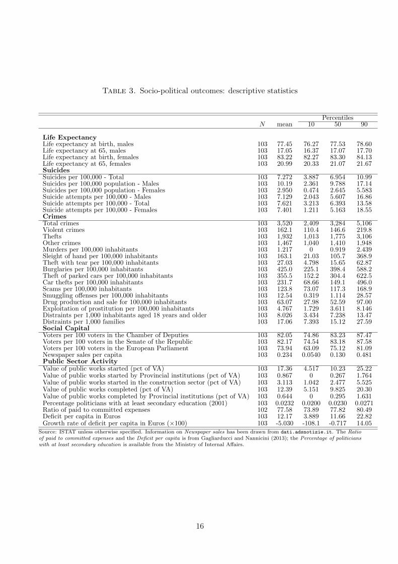
Table 3. Socio-political outcomes: descriptive statistics
PercentilesN mean 10 50 90
Life ExpectancyLife expectancy at birth, males 103 77.45 76.27 77.53 78.60Life expectancy at 65, males 103 17.05 16.37 17.07 17.70Life expectancy at birth, females 103 83.22 82.27 83.30 84.13Life expectancy at 65, females 103 20.99 20.33 21.07 21.67SuicidesSuicides per 100,000 - Total 103 7.272 3.887 6.954 10.99Suicides per 100,000 population - Males 103 10.19 2.361 9.788 17.14Suicides per 100,000 population - Females 103 2.950 0.474 2.645 5.583Suicide attempts per 100,000 - Males 103 7.129 2.043 5.607 16.86Suicide attempts per 100,000 - Total 103 7.621 3.213 6.393 13.58Suicide attempts per 100,000 - Females 103 7.401 1.211 5.163 18.55CrimesTotal crimes 103 3,520 2,409 3,284 5,106Violent crimes 103 162.1 110.4 146.6 219.8Thefts 103 1,932 1,013 1,775 3,106Other crimes 103 1,467 1,040 1,410 1,948Murders per 100,000 inhabitants 103 1.217 0 0.919 2.439Sleight of hand per 100,000 inhabitants 103 163.1 21.03 105.7 368.9Theft with tear per 100,000 inhabitants 103 27.03 4.798 15.65 62.87Burglaries per 100,000 inhabitants 103 425.0 225.1 398.4 588.2Theft of parked cars per 100,000 inhabitants 103 355.5 152.2 304.4 622.5Car thefts per 100,000 inhabitants 103 231.7 68.66 149.1 496.0Scams per 100,000 inhabitants 103 123.8 73.07 117.3 168.9Smuggling offenses per 100,000 inhabitants 103 12.54 0.319 1.114 28.57Drug production and sale for 100,000 inhabitants 103 63.07 27.98 52.59 97.00Exploitation of prostitution per 100,000 inhabitants 103 4.767 1.729 3.611 8.146Distraints per 1,000 inhabitants aged 18 years and older 103 8.026 3.434 7.238 13.47Distraints per 1,000 families 103 17.06 7.393 15.12 27.59Social CapitalVoters per 100 voters in the Chamber of Deputies 103 82.05 74.86 83.23 87.47Voters per 100 voters in the Senate of the Republic 103 82.17 74.54 83.18 87.58Voters per 100 voters in the European Parliament 103 73.94 63.09 75.12 81.09Newspaper sales per capita 103 0.234 0.0540 0.130 0.481Public Sector ActivityValue of public works started (pct of VA) 103 17.36 4.517 10.23 25.22Value of public works started by Provincial institutions (pct of VA) 103 0.867 0 0.267 1.764Value of public works started in the construction sector (pct of VA) 103 3.113 1.042 2.477 5.525Value of public works completed (pct of VA) 103 12.39 5.151 9.825 20.30Value of public works completed by Provincial institutions (pct of VA) 103 0.644 0 0.295 1.631Percentage politicians with at least secondary education (2001) 103 0.0232 0.0200 0.0230 0.0271Ratio of paid to committed expenses 102 77.58 73.89 77.82 80.49Deficit per capita in Euros 103 12.17 3.889 11.66 22.82Growth rate of deficit per capita in Euros (×100) 103 -5.030 -108.1 -0.717 14.05
Source: ISTAT unless otherwise specified. Information on Newspaper sales has been drawn from dati.adsnotizie.it. The Ratioof paid to committed expenses and the Deficit per capita is from Gagliarducci and Nannicini (2013); the Percentage of politicianswith at least secondary education is available from the Ministry of Internal Affairs.
16

(anonymised) surnames available for Italy, the closest to a census. As discussed, surname
distributions are very skewed. To the extent that those distributions – the complex result of
fertility processes, (assortative) mating and migration patterns – are similar, any differences in
the ICS will reflect differences in mobility.
As it is well known that the Pareto distribution – completely characterized by two moments,
the Gini coefficient and the number of persons per surname – provides a good approximation
of the surname distributions in many societies (Fox and Lasker (1983)), Figure 1 plots, for
every province, the Gini coefficient and the average number of persons per surname.8 While
the Gini indices seem relatively homogeneous within the range [0.6, 0.9], the average number
of persons per surname spans between 10 and 50. To enhance cross-province comparability,
as explained in Section 2.2, we also calculate the ICS measures concentrating on the right
tail of the distribution of surnames, i.e. in each province we focus on the individuals whose
surname contains less than a certain amount of people (we experiment with 15, 20, 25 and 30).
The idea behind this strategy is that, for these sub-populations, surnames measure the same
degree of “family connectivity” in different provinces. Thus, the mapping from these measures
into family relationship is very similar (if not identical) across provinces. In other words, by
insuring the same surname distributions we insure that we are measuring the same across all
provinces. We are comparing alike with alike, and the differences in ICS reflect differences in
the intergenerational persistence of the income process across provinces. Figures 1(a) to 1(e)
show the Gini coefficient and the number of persons per surname for the whole population
and for the tails of the distribution. These figures show that indeed we gain in cross-provincial
comparability when focusing on the tails of the distribution as the surname distribution becomes
essentially identical in all of them. We are thus quite confidant that (at least when using the
tails) surnames map family relationship in the same manner in all provinces, and that the
mapping from ICS to income persistence is the same in all of them.
In any case, just for the possibility that differences in migration patterns could account for
difference in this mapping from surnames to families, we also do the exercise of calculating
for each province the ICS of the tails of the surname distribution but only for the 50% of the
8Appendix A.1 shows the surname distributions for the 20 Italian regions. The 103 provincial surnamedistributions provide a very similar visual impression.
17

Table 4. ICS measures based on taxable income: descriptive statistics
PercentilesN Mean St.Dev. 10 50 90
ICS based on taxable income, 103 0.0244 0.00847 0.0147 0.0233 0.0360ICS based on taxable income, tail 30 103 0.0450 0.0169 0.0292 0.0388 0.0721ICS based on taxable income, tail 25 103 0.0472 0.0177 0.0308 0.0411 0.0749ICS based on taxable income, tail 20 103 0.0498 0.0188 0.0327 0.0420 0.0800ICS based on taxable income, tail 15 103 0.0532 0.0204 0.0340 0.0451 0.0845
population with the most local surnames as defined in section 2.3.
5.1 Empirical measures of the ICS
This section presents the ICS measures calculated on the population of Italian males taxpayer
described in Section 4.1. We first calculate, for each province, the ICS measure on the full male
population taking the difference between the R2 of a regression of (log) taxable income on a full
set of surname dummies (and age dummies) and the average R2 of M identical regressions9 in
which surnames are previously randomly reshuffled across individuals. This allows to control
for the fact that (part of) the variance of income may be mechanically explained by the very
inclusion of such a large set of dummies.
Descriptive statistics for ICS measures based on taxable income are reported in Table 4.
The first row refers to the ICS calculated on the full population. Subsequent rows report
the ICS restricting the population to the individuals with the least frequent surnames, i.e.
those containing less than 30, 25, 20, and 15 persons. Overall, the Table shows that there is
substantial variation in the ICS across provinces: the baseline ICS of the province at the 90th
percentile (Latina) is almost 2.5 higher than the ICS of the province at the 10th percentile
(Macerata). Table 4 also shows – not surprisingly – that the ICS monotonically increases when
focusing on more and more infrequent surnames.
Figure 2 provides a geographical breakdown of estimates of social mobility and shows,
consistently across the different ICS measures, that social mobility is higher in the Centre and
North (highest in the North-West) and lower in the South (lowest in the South-West).
9We set M = 10 and experiment with more replications without changes in the results.
18

010
2030
4050
Ave
rage
per
sons
per
sur
nam
e
0 .1 .2 .3 .4 .5 .6 .7 .8 .9 1Gini Coefficient
(a) All Individuals
010
2030
4050
Ave
rage
per
sons
per
sur
nam
e
0 .1 .2 .3 .4 .5 .6 .7 .8 .9 1Gini Coefficient
(b) Individuals with surnames with < 30 peo-ple
010
2030
4050
Ave
rage
per
sons
per
sur
nam
e
0 .1 .2 .3 .4 .5 .6 .7 .8 .9 1Gini Coefficient
(c) Individuals with surnames with < 25 peo-ple
010
2030
4050
Ave
rage
per
sons
per
sur
nam
e
0 .1 .2 .3 .4 .5 .6 .7 .8 .9 1Gini Coefficient
(d) Individuals with surnames with < 20 peo-ple
010
2030
4050
Ave
rage
per
sons
per
sur
nam
e
0 .1 .2 .3 .4 .5 .6 .7 .8 .9 1Gini Coefficient
(e) Individuals with surnames with < 15 peo-ple
Figure 1. Comparability of surname distributions across provinces.
19

Figure 2. ICS measures based on taxable income by geographical areas
Table 5. ICS measures based on taxable income exploiting how local surnames are: descriptivestatistics
PercentilesN Mean St.Dev. 10 50 90
ICS based on taxable income, local 103 0.0239 0.00991 0.0125 0.0217 0.0390ICS based on taxable income, local and tail 30 103 0.0504 0.0189 0.0328 0.0464 0.0700ICS based on taxable income, local and tail 25 103 0.0536 0.0201 0.0333 0.0493 0.0728ICS based on taxable income, local and tail 20 103 0.0581 0.0218 0.0368 0.0531 0.0796ICS based on taxable income, local and tail 15 103 0.0633 0.0243 0.0410 0.0565 0.0888
Table 5 shows descriptive statistics for ICS measures based on taxable income and calculated
for the fraction of individuals in the top 50 percent of the distribution of the LocalDegree(s, r)
Index in every province, as described in Section 2.3. From the second row (as in Table 4) we
further restrict the population to the most infrequent surnames. Overall, we again see marked
variation across provinces and a monotonically increasing pattern of the ICS as we restrict to
more and more infrequent surnames. The geographical breakdown (not reported) of the local
ICS provides a picture similar to the one that emerges from Figure 2.
Table 6 displays the pairwise correlations between all the ICS measures shown in Tables 4
and 5. Correlations are all very high (and all significantly different from zero). In particular,
it is reassuring to see that the Full male population ICS and the Local ICS are very correlated
(0.9068), implying that differential migration patterns across provinces are not likely to be a
20

Table 6. Pairwise correlations across ICS measures
Full ICS ICS-15 ICS-20 ICS-25 ICS-30 Local ICS Local ICS-15 Local ICS-20 Local ICS-25 Local ICS-30
Full ICS 1.0000ICS-15 0.6912 1.0000ICS-20 0.6965 0.9957 1.0000ICS-25 0.6899 0.9924 0.9965 1.0000ICS-30 0.7019 0.9877 0.9944 0.9970 1.0000Local ICS 0.9068 0.5356 0.5350 0.5305 0.5391 1.0000Local ICS-15 0.5650 0.8510 0.8520 0.8575 0.8531 0.5058 1.0000Local ICS-20 0.5936 0.8604 0.8647 0.8714 0.8682 0.5384 0.9880 1.0000Local ICS-25 0.6262 0.8586 0.8651 0.8745 0.8729 0.5713 0.9793 0.9915 1.0000Local ICS-30 0.6408 0.8536 0.8640 0.8728 0.8750 0.5835 0.9694 0.9831 0.9921 1.0000
Notes: Full ICS refers to the ICS calculated with the full male population ICS. All other ICS are calculated with the relevant tailof the surname distribution. Local ICS is calculated with only the 50% of the population with the most local surnames.
major source of concern.
5.1.1 Correlation ICS and traditional measure of IM
In this section we compare our ICS measure with a traditional measure of intergenerational
mobility. However, for Italy there is no extensive longitudinal data set that would allow us
to measure mobility at the province level using traditional methods. Some papers have used
data from the Survey on Household Income and Wealth (SHIW) from the Bank of Italy, which
consists of repeated cross-sections with some retrospective information on fathers characteristics
to obtain measures of mobility.10 However, given the limited number of observations in the
SHIW data at the province level, it is not possible to obtain reliable estimates of the traditional
measure at such a detailed geographical level. For this reason, we calculate both the traditional
measure – following Checchi, Fiorio, and Leonardi (2013) – and ours at a more aggregate levels,
namely 20 regions and 5 broad areas, in order to be able to make a meaningful comparison.
Table 7 reports the correlation between the traditional measure and our surname-based
measure. Before interpreting the reported correlations we need to be aware of the several
caveats here. First, the very small number of observations and the fact that one measure is on
income and the other one on years of education. Still, despite this, our surname-based measure
and the traditional one are positively correlated and some of them (even if not significant)
have high values. When we drop 25% of the regions with least observations in the SHIW,
10 See Piraino (2007), Mocetti (2007) and Checchi, Fiorio, and Leonardi (2013). The only other data sourceused to estimate mobility in Italy is a survey conducted in 1985 on occupations with retrospective informationon parents (Checchi, Ichino, and Rustichini, 1999).
21

Table 7. Pairwise correlations between ICS and traditional intergenerational elasticity
Full ICS ICS-30 ICS-25 ICS-20 ICS-15
Traditional IM measure 0.7878 0.7310 0.7225 0.7233 0.7297(0.1136) (0.1605) (0.1680) (0.1673) (0.1617)
Level aggregation & observations 5 areas 5 areas 5 areas 5 areas 5 areas
Traditional IM measure 0.2314 0.2527 0.2623 0.2836 0.2799(0.3264) (0.2824) (0.2639) (0.2257) (0.2320)
Level aggregation & observations 20 regions 20 regions 20 regions 20 regions 20 regions
Traditional IM measure 0.4752 0.6626* 0.6875* 0.6930* 0.6980*(0.0734) (0.0071) (0.0046) (0.0042) (0.0038)
Level aggregation 20 regions 20 regions 20 regions 20 regions 20 regionsObservations (exclude 5 regions with least observations) 15 regions 15 regions 15 regions 15 regions 15 regions
Pairwise correlations and p-values in parentheses. (*) indicates significance at the 5% level or better. The traditional IM elasticityas in Checchi, Fiorio, and Leonardi (2013). ICS measures as in tables 4 and 5. Full ICS refers to the ICS calculated with the fullmale population ICS. All other ICS are calculated with the relevant tail of the surname distribution. Local ICS is calculated withonly the 50% of the population with the most local surnames.
then the correlations become significant (these are very small regions with a small number of
observations). Overall, this is reassuring as it shows that indeed our approach is capturing
the different mobility patterns across geographical areas. We can, thus, confidently use use our
province-level ICS to explore how social mobility correlates with a number of meaningful macro
outcomes.
6 Intergenerational mobility and macroeconomic outcomes
We now turn to the analysis of the correlations between the ICS measures and the battery of
(log) macroeconomic outcomes described in Section 4.2. To organize the analysis we divide the
macro variables described in section 4.2 in two groups, the first one relating to purely economic
variables, and the second to socio-political ones.
6.1 Correlating ICS and Economic Outcomes
Table 8 presents, in each column, the pairwise correlations between different ICS measures (full
male population in column 1 and tail-based measure from column 2) and a number of meaningful
economic outcomes. Recalling that a higher ICS implies lower mobility, the table shows that
22

Figure 3. Scatter plots of ICS-30 and “good” economic outcomes
“good” economic outcomes measured at the province level, such as value added, wealth, income,
employment rates, participation rates, imports and exports, are consistently positively and
significantly related to higher mobility; instead “negative” outcomes, such as unemployment
rates of different socio-economic groups and shares of low-educated young individuals, are
related to lower mobility. This pattern emerges consistently across the different types of ICS
displayed in the different columns.
This is our first qualitative result: intergenerational mobility correlates positively with
“good” economic outcomes, even controlling for identical institutional set-up. Where (eco-
nomic) things are good, mobility is high.
In order to provide a visual representation of this result we divide the economic variables in
two groups of “good” and “bad” variables (see table 9 for the categorization of each variable).
We then plot the scatter plots of the “good” and “bad” variables in Figures 3 and 4 respectively.
Moreover, in Figure 5 we plot the value of the correlations (for ICS-30) and their P-values for
23

Table 8. Pairwise correlations between ICS from Taxable Income and Macro outcomes, Men
Full ICS ICS-30 ICS-25 ICS-20 ICS-15Economic ActivityValue added per capita -0.3353* -0.5618* -0.5618* -0.5626* -0.5681*
(0.0005) (0.0000) (0.0000) (0.0000) (0.0000)Value added per full time equivalent worker -0.2260* -0.2446* -0.2411* -0.2338* -0.2419*
(0.0217) (0.0128) (0.0141) (0.0175) (0.0138)Protested cheques per 1000 inhabitants 0.2240* 0.3724* 0.3646* 0.3817* 0.3692*
(0.0229) (0.0001) (0.0002) (0.0001) (0.0001)Labour marketUnemployment rate 0.4303* 0.6490* 0.6434* 0.6498* 0.6551*
(0.0000) (0.0000) (0.0000) (0.0000) (0.0000)Unemployment rate (males) 0.4352* 0.6560* 0.6512* 0.6582* 0.6636*
(0.0000) (0.0000) (0.0000) (0.0000) (0.0000Unemployment rate (females) 0.4245* 0.6487* 0.6427* 0.6488* 0.6539*
(0.0000) (0.0000) (0.0000) (0.0000) (0.0000)Unemployment rate (age 15-24) 0.4414* 0.5775* 0.5720* 0.5799* 0.5879*
(0.0000) (0.0000) (0.0000) (0.0000) (0.0000Long-term unemployment rate (> 12 months) 0.4071* 0.5776* 0.5685* 0.5803* 0.5815*
(0.0000) (0.0000) (0.0000) (0.0000) (0.0000)Employment rate -0.5076* -0.6679* -0.6642* -0.6751* -0.6781*
(0.0000) (0.0000) (0.0000) (0.0000) (0.0000Employment rate (males) -0.5053* -0.5791* -0.5763* -0.5880* -0.5939*
(0.0000) (0.0000) (0.0000) (0.0000) (0.0000)Employment rate (females) -0.4914* -0.7068* -0.7026* -0.7125* -0.7133*
(0.0000) (0.0000) (0.0000) (0.0000) (0.0000Employment rate (age 15-24) -0.4808* -0.6338* -0.6328* -0.6441* -0.6524*
(0.0000) (0.0000) (0.0000) (0.0000) (0.0000)Employment rate (high school aged 25-64) -0.4780* -0.7168* -0.7111* -0.7194* -0.7208*
(0.0000) (0.0000) (0.0000) (0.0000) (0.0000Employment rate (college degree aged 25-64) -0.3912* -0.5902* -0.5895* -0.6029* -0.6115*
(0.0000) (0.0000) (0.0000) (0.0000) (0.0000)Participation rate (age 15-64) -0.4327* -0.6576* -0.6593* -0.6690* -0.6702*
(0.0000) (0.0000) (0.0000) (0.0000) (0.0000Participation rate (males aged 15-64) -0.3551* -0.4141* -0.4181* -0.4286* -0.4331*
(0.0002) (0.0000) (0.0000) (0.0000) (0.0000)Participation rate (females aged 15-64) -0.4323* -0.7009* -0.7016* -0.7106* -0.7103*
(0.0000) (0.0000) (0.0000) (0.0000) (0.0000Participation rate (age 15-24) -0.5307* -0.5386* -0.5333* -0.5501* -0.5543*
(0.0000) (0.0000) (0.0000) (0.0000) (0.0000)OpennessImports to values added -0.2581* -0.3466* -0.3427* -0.3491* -0.3541*
(0.0085) (0.0003) (0.0004) (0.0003) (0.0002)Exports to values added -0.4260* -0.5761* -0.5714* -0.5753* -0.5798*
(0.0000) (0.0000) (0.0000) (0.0000) (0.0000)EducationIndividuals with at most secondary school (aged 25-26) 0.1741 0.4597* 0.4567* 0.4498* 0.4488*per 100 same age individuals (0.0786) (0.0000) (0.0000) (0.0000) (0.0000)Early school dropout (aged 18-24) 0.1843 0.4589* 0.4437* 0.4352* 0.4177*per 100 same age individuals (0.0624) (0.0000) (0.0000) (0.0000) (0.0000)InequalityLog 90/10 income percentile 0.0381 0.2311* 0.2435* 0.2510* 0.2473*
(0.7022) (0.0188) (0.0132) (0.0105) (0.0118)
Notes: Pairwise correlations and p-values in parentheses. (*) indicates significance at the 5% level or better. Full ICS refers to theICS calculated with the full male population ICS. All other ICS are calculated with the relevant tail of the surname distribution.Local ICS is calculated with only the 50% of the population with the most local surnames.
24

Table 9. Good and Bad Economic Outcomes
Good Economic OutcomesValue added per capitaValue added per full time equivalent workerEmployment rateEmployment rate (males)Employment rate (females)Employment rate aged 15-24 yearsEmployment rate (high school aged 25-64)Employment rate (college degree aged 25-64)Participation rate in the age group 15-64 yearsParticipation rate in the age group 15-64 years (males)Participation rate in the age group 15-64 years (females)Participation rate in the age group 15-24 yearsPercentage politicians with at least secondary educationLife expectancy at birth (males)Life expectancy at 65 (males)Life expectancy at birth (females)Life expectancy at 65 (females)Imports to value addedExports to value addedRatio of paid to committed expenses
Bad Economic OutcomesUnemployment rateUnemployment rate (males)Unemployment rate (females)Unemployment rate in the age group 15-24 yearsLong-term unemployment rate (12 months or more) - To-talDeficit per capita in EuroEarly school dropout aged 18-24 per 100 same age individ-ualsIndividuals aged 25-26 with at most secondary school per100 same age individualsGrowth rate of deficit per capita in EuroProtested cheques per 1000 inhabitants
Figure 4. Scatter plots of ICS-30 and “bad” economic outcomes
25

Figure 5. Pairwise correlations between ICS-30 economic outcomes and their P-values
those variables. It is clear from those graphs that effectively, high mobility happens in places
where good (economic) things happen.
The relationship between intergenerational mobility and inequality has a special interest on
its own. A clear positive correlation between the intergenerational elasticity of earnings and the
degree of cross-sectional inequality – named “the Great Gatsby Curve” – exists across countries.
This correlation has become the focus of a large public debate (Corak, 2013; Krueger, 2012)
which often interprets it as the result of institutional differences: inequality and the prevalence
of inheritance being low in countries with more government intervention as the Nordic countries,
and high in laissez-faire societies like the Anglo-Saxon countries.
We explore the existence of a Great Gatsby Curve within Italy using as a measure of cross-
sectional inequality the 90/10 percentile ratio calculated from our tax data. We correlate it
with our ICS measures (see the last row of Table 8) and find our second qualitative result: in
provinces where income inequality is lower, inheritance is less prevalent. We plot the Italian
Great Gatsby curve in Figure 6, and report the correlation coefficient (and it P-value) in Figure
5 together with the other economic outcomes mentioned above.
26

Figure 6. The Italian Great Gatsby Curve. Scatter plot of ICS-30 and inequality
6.2 Socio-Political Variables
We now turn to how socio-political aggregate variables correlate with intergenerational mobility
at the province level. In table 10 we present the correlation coefficients between our ICS
measures and a battery of socio-political variables categorized in five groups.
A mere glimpse at the table shows that we can not make the same claim as with the
economic variables. Thus, our third qualitative result: it is not the case that more social
mobility is systematically associated with better social outcomes.
This can be also seen in the scatter plots for each socio-political group of variables (grouped
as explained in section 4.2): figures 7, 8 9, 10, and 11.
Looking at them one by one, the following evidence emerges:
• Social mobility correlates with higher life expectancy for females, but not for males.
• On the other hand, social mobility correlates with higher suicide rates (in essentially any
possible categorization of suicides).
• as to crime, while higher mobility is associated to higher total crime rates and higher
property crime rates (thefts, sleight of hand, burglaries, exploitation of prostitution),
murders and smuggling are related to lower mobility. It is not possible to get any clearcut
conclusion on this set of outcomes. For instance, “theft of parked cars” and “theft of
27

Table 10. Pairwise correlations of ICS from Taxable Income and Socio-Political variables, Men
Full ICS ICS-30 ICS-25 ICS-20 ICS-15Life ExpectancyLife expectancy at birth (males) -0.1297 -0.0197 -0.0169 -0.0010 -0.0115
(0.1916) (0.8438) (0.8657) (0.9917) (0.9079)Life expectancy at 65 (males) -0.0395 0.0725 0.0765 0.0912 0.0914
(0.6919) (0.4669) (0.4426) (0.3593) (0.3587)Life expectancy at birth (females) -0.4136* -0.3695* -0.3662* -0.3590* -0.3616*
(0.0000) (0.0001) (0.0001) (0.0002) (0.0002)Life expectancy at 65 (females) -0.4213* -0.4957* -0.4910* -0.4863* -0.4882*
(0.0000) (0.0000) (0.0000) (0.0000) (0.0000)SuicidesSuicides per 100,000 individuals -0.2296* -0.4801* -0.4673* -0.4860* -0.4754*
(0.0197) (0.0000) (0.0000) (0.0000) (0.0000)Suicides per 100,000 individuals (males) 0.0209 -0.3120* -0.3061* -0.3197* -0.3174*
(0.8354) (0.0015) (0.0018) (0.0011) (0.0012)Suicides per 100,000 individuals (females) -0.0711 -0.3094* -0.3068* -0.3247* -0.3226*
(0.4956) (0.0024) (0.0026) (0.0014) (0.0015)Suicides attempts per 100,000 individuals -0.0395 -0.3095* -0.3057* -0.3232* -0.3286*
(0.6924) (0.0015) (0.0017) (0.0009) (0.0007)Suicides attempts per 100,000 individuals (males) 0.0199 -0.2871* -0.2861* -0.3034* -0.3008*
(0.8438) (0.0038) (0.0039) (0.0021) (0.0024)Suicides attempts per 100,000 individuals (females) 0.0395 -0.2116* -0.2116* -0.2274* -0.2420*
(0.6982) (0.0355) (0.0355) (0.0236) (0.0158)CrimesTotal crimes -0.2444* -0.2297* -0.2288* -0.2317* -0.2499*
(0.0128) (0.0196) (0.0201) (0.0185) (0.0109)Violent crimes -0.1378 0.0365 0.0364 0.0324 0.0331
(0.1652) (0.7146) (0.7154) (0.7454) (0.7399)Thefts -0.3534* -0.2496* -0.2475* -0.2558* -0.2781*
(0.0003) (0.0110) (0.0117) (0.0091) (0.0045)Other crimes 0.0676 -0.0967 -0.0991 -0.0947 -0.0950
(0.4974) (0.3312) (0.3195) (0.3415) (0.3400)Murders per 100,000 inhabitants 0.3235* 0.2949* 0.2860* 0.2934* 0.2839*
(0.0017) (0.0043) (0.0057) (0.0045) (0.0061)Sleight of hand per 100,000 inhabitants -0.2562* -0.3893* -0.3888* -0.3908* -0.4041*
(0.0090) (0.0000) (0.0000) (0.0000) (0.0000)Breaking and entering per 100,000 inhabitants -0.0453 0.2351* 0.2315* 0.2284* 0.2060*
(0.6498) (0.0168) (0.0186) (0.0203) (0.0368)Burglaries per 100,000 inhabitants -0.4595* -0.5286* -0.5292* -0.5306* -0.5521*
(0.0000) (0.0000) (0.0000) (0.0000) (0.0000)Theft of parked cars per 100,000 inhabitants -0.4320* -0.4204* -0.4118* -0.4169* -0.4324*
(0.0000) (0.0000) (0.0000) (0.0000) (0.0000)Car thefts per 100,000 inhabitants 0.0019 0.2886* 0.2785* 0.2787* 0.2651*
(0.9846) (0.0031) (0.0044) (0.0044) (0.0068)Scams per 100,000 inhabitants -0.1815 -0.2657* -0.2605* -0.2704* -0.2782*
(0.0666) (0.0067) (0.0079) (0.0057) (0.0044)Smuggling offences per 100,000 inhabitants 0.2948* 0.3096* 0.3114* 0.3139* 0.3127*
(0.0026) (0.0015) (0.0014) (0.0013) (0.0014)Drug production and sale for 100,000 inhabitants 0.0173 -0.1124 -0.1174 -0.1034 -0.1159
(0.8626) (0.2585) (0.2374) (0.2985) (0.2436)Exploitation of prostitution per 100,000 inhabitants -0.3502* -0.4711* -0.4739* -0.4645* -0.4697*
(0.0003) (0.0000) (0.0000) (0.0000) (0.0000)Distraints per 1,000 inhabitants aged ≥18 years 0.0821 0.0949 0.0789 0.0905 0.0853
(0.4095) (0.3406) (0.4280) (0.3632) (0.3915)Distraints per 1,000 families 0.0989 0.1597 0.1446 0.1560 0.1510
(0.3205) (0.1072) (0.1449) (0.1157) (0.1278)Social Capital MeasuresVoters per 100 voters in the Chamber of Deputies -0.4287* -0.6199* -0.6224* -0.6278* -0.6372*
(0.0000) (0.0000) (0.0000) (0.0000) (0.0000)Voters per 100 voters in the Senate -0.2912* -0.3857* -0.3831* -0.3902* -0.3943*
(0.0028) (0.0001) (0.0001) (0.0000) (0.0000)Voters per 100 voters in the European Parliament -0.4703* -0.5941* -0.5939* -0.5928* -0.5943*
(0.0000) (0.0000) (0.0000) (0.0000) (0.0000)Newspaper sales per capita -0.2372* -0.4156* -0.4151* -0.4136* -0.4269*
(0.0159) (0.0000) (0.0000) (0.0000) (0.0000)Public SectorValue of public works started (pct of VA) 0.1866 0.1935 0.1847 0.1730 0.1745
(0.0592) (0.0502) (0.0618) (0.0805) (0.0780)Value of public works started by Provincial institutions 0.2260* 0.3401* 0.3467* 0.3482* 0.3542*(pct of VA) (0.0496) (0.0026) (0.0022) (0.0021) (0.0017)Value of public works started in the construction sector 0.1659 0.3324* 0.3348* 0.3319* 0.3477*(pct of VA) (0.0939) (0.0006) (0.0005) (0.0006) (0.0003)Value of public works completed 0.2823* 0.2325* 0.2305* 0.2289* 0.2383*(pct of VA) (0.0039) (0.0181) (0.0192) (0.0200) (0.0153)Value of public works completed by Provincial institutions 0.2504* 0.3478* 0.3613* 0.3548* 0.3734*(pct of VA) (0.0281) (0.0019) (0.0012) (0.0015) (0.0008)Percentage of politicians with at least secondary education 0.0419 0.2468* 0.2531* 0.2565* 0.2366*
(0.6740) (0.0120) (0.0099) (0.0089) (0.0161)Ratio of paid to committed expenses 0.0333 -0.0802 -0.0708 0.0619 -0.0477
(0.7385) (0.4209) (0.4775) (0.5345) (0.6321)Deficit per capita in Euro -0.0987 0.0177 0.0164 0.0042 0.0051
(0.3361) (0.8635) (0.8737) (0.9672) (0.9608)Growth rate of deficit per capita in Euro 0.1032 0.1980 0.2004 0.2011 0.2101
(0.5101) (0.2032) (0.1977) (0.1960) (0.1763)
Notes: Pairwise correlations and p-values in parentheses. (*) indicates significance at the 5% level or better.28

Figure 7. Scatter plots of ICS-30 and life expectancy
Figure 8. Scatter plots of ICS-30 and suicides
29

Figure 9. Scatter plots of ICS-30 and crime
cars” exhibit opposite correlations.
• Higher social mobility correlates positively with all the “social capital” proxies available:
voters turnout in different types of elections and newspaper sales per capita. For these
variables, as for the economic ones, good outcomes are related to higher social mobility
while bad ones are related to lower mobility.
• Finally, we also correlate our measures of mobility with measures of public sector activity
at the provincial level. We include them here, and not with the economic variables,
because they also capture the reaction of the local governments to the economic conditions
of the local areas (intensity of public sector activity measured as the value of the public
works started), and the quality of the political system as measured by the schooling level
of the politicians and by the budget deficit.
As we said, the picture is much less clear-cut than in the case of the economic variables. In
30

Figure 10. Scatter plots of ICS-30 and social capital
Figure 11. Scatter plots of ICS-30 and public sector activity
31

Figure 12. Pairwise correlations between ICS-30 and Socio-Political Variables.
figure 12 we plot the correlations and P-value for all socio-political variables grouped in the 5
groups just described. While some variables which are obviously desirable (like life expectancy
for females) are clearly positive related with mobility, others that are obviously negative (like
suicide rates) are also positively correlated to intergenerational mobility, and crime is all over
the place.
Perhaps not surprisingly, the interaction between mobility and these social variables appears
much more complex and unpredictable the interaction with the economic ones, where mobility
is systematically associated to desirable outcomes.
7 Conclusions
Is intergenerational mobility a good thing? Well, of course it is. It has to do with equality
of opportunities and it is clearly a desirable feature of any society. But things do not often
come for free. It could be well the case that societies that show high mobility could in principle
suffer from undesirable outcomes. Actually, it is often suggested that this is the case, given the
32

evidence that intergenerational mobility in the US is low (albeit with large regional variation,
as we know since recently (Chetty, Hendren, Kline, and Saez, 2014)), while income per-capita
(along with many other desirable economic dimensions) is high.
In this paper we use Italian data to correlate intergenerational mobility with macroeconomic
and social variables at the provincial level. We believe that the advantages of using Italy are
manifold:
1. Italy is a relatively large country, composed of many different local entities which are
extraordinarily heterogeneous in their economic and social performances.
2. The institutional framework is the same in all provinces. Whatever makes mobility and
other outcomes high in one place and low in others is not the difference in the rules of
the game.
3. The surname distribution is very similar across provinces, and when concentrating on the
tails of the surname distributions, it is essentially identical. Thus, we can reliably use
the ICS (a measure of intergenerational mobility developed by Guell, Rodrıguez Mora,
and Telmer (2014)) to compare intergenerational mobility across provinces because in
all of them the mapping from surnames to family relationships is very similar. Thus, in
all of them the mapping between the persistence of the income process and the ICS is
identical. Therefore, comparing the ICS across provinces is akin to compare the degree
of persistence of the income process across generations.
The measurement exercise shows that intergenerational mobility is larger in the North, and
lower in the South of Italy. Reassuringly, our ICS measure correlates pretty well with existing
measures of mobility (albeit these are based on scarce data and are unsuitable to explore the
correlation between mobility and other outcomes).
Our key findings are as follows:
1. Mobility correlates positively with desirable economic outcomes and negatively with un-
desirable ones.
33

2. The latter includes economic inequality. Thus, there exists a Great Gatsby curve for
Italian provinces even if there are no institutional differences across them.
3. The clear and systematic pattern that shows up for economic outcomes does not exist for
socio-political outcomes.
We see as an advantage of our approach that the institutional framework is the same across
all units of observation. Nevertheless, it is reasonable to expect that part of the observed
differences in economic (and socio-political) outcomes and intergenerational mobility across
countries may be due in differences in the institutional framework. More or less redistribution.
More or less meritocracy. More or less availability of public education. All these institutional
characteristics are extremely likely to affect the degree of intergenerational mobility and the
performance of the economy. Our intention is to use the methodology that we have developed
here in order to look at the effect of the differences in the institutional setting in further research
focused on cross-country comparisons.
References
Anelli, M. and G. Peri (2013). Peer Gender Composition and Choice of College Major. NBERWorking Papers 18744, National Bureau of Economic Research, Inc.
Bjorklund, A., T. Eriksson, M. Jantti, O. Raaum, and E. Osterbacka (2002). Brother correla-tions in earnings in Denmark, Finland, Norway, and Sweden compared to the United States.Journal of Population Economics 15 (4), 757–772.
Bjorklund, A. and M. Jantti (1997). Intergenerational income mobility in Sweden compared tothe United States. American Economic Review 87 (5), 1009–1018.
Black, S. E. and P. J. Devereux (2011). Recent Developments in Intergenerational Mobility.in Orley C. Ashenfelter and David Card (eds.), Handbook of Labor Economics, Volume 4B,Amsterdam: North-Holland, pp. 1487-1541.
Braga, M., M. Paccagnella, and M. Pellizzari (2014). The academic and labor market returnsof university professors. The Journal of Labor Economics.
Checchi, D., C. V. Fiorio, and M. Leonardi (2013). Intergenerational persistence in educationalattainment in Italy. Economics Letters 118, 229–232.
Checchi, D., A. Ichino, and A. Rustichini (1999). More equal but less mobile? Educationfinancing and intergenerational mobility in Italy and in the U.S. Journal of Public Eco-nomics 74 (3), 351–93.
Chetty, R., N. Hendren, P. Kline, and E. Saez (2014). Where is the land of opportunity?the geography of intergenerational mobility in the United States. Quarterly Journal of Eco-nomics 129 (4), 1553–1623.
34

Comi, S. (2003). Intergenerational mobility in Europe: evidence from ECHP. DepartmentalWorking Papers 2003-03, Department of Economics, Management and Quantitative Methodsat Universita degli Studi di Milano.
Corak, M. (2013). Inequality from Generation to Generation: The United States in Comparison.Robert Rycroft editor, The Economics of Inequality, Poverty, and Discrimination in the 21stCentury, ABC-CLIO.
Couch, K. A. and T. A. Dunn (1997). Intergenerational correlations in labor market status: Acomparison of the United States and Germany. Journal of Human Resources 32 (1), 210–32.
Fox, W. R. and G. W. Lasker (1983). The distribution of surname frequencies. InternationalStatistical Review 51 (1), 81–87.
Gagliarducci, S. and T. Nannicini (2013, April). Do better paid politicians perform better?disentangling incentives from selection. Journal of the European Economic Association 11 (2),369–398.
Grawe, N. D. (2004). Intergenerational mobility for whom? The experience of high- and low-earnings son in international perspective. in Miles Corak (ed.), Generational Income Inequal-ity, Cambridge University Press, pp.58-89.
Guell, M., J. V. Rodrıguez Mora, and C. I. Telmer (2014). The informational content ofsurnames, the evolution of intergenerational mobility and assortative mating. The Review ofEconomic Studies , Forthcoming.
Haider, S. and G. Solon (2006). Life-cycle variation in the association between current andlifetime earnings. The American Economic Review 96 (4), 1308–1320.
Hertz, T. (2007). Trends in the intergenerational elasticity of family income in the UnitedStates. Industrial Relations 46 (1), 22–50.
Krueger, A. B. (2012). The rise and consequences of inequality in the United States. Speechof the Chairman of Council of Economic Advisers at the Center for American Progress onJanuary 12th, 2012.
Lee, C.-I. and G. Solon (2009). Trends in intergenerational income mobility. Review of Eco-nomics and Statistics 91 (November), 766–772.
Mocetti, M. (2007). Intergenerational earnings mobility in Italy. The B.E. Journal of EconomicAnalysis & Policy 7,(Iss. 2 (Topics)), 1935–1682.
Piraino, P. (2007). Comparable estimates of intergenerational income mobility in Italy. TheB.E. Journal of Economic Analysis & Policy 7,(Iss. 2 (Topics)), 1935–1682.
Solon, G. (1992). Intergenerational income mobility in the United States. American EconomicReview 82 (3), 393–408.
Solon, G. (1999). Intergenerational Mobility in the Labor Market. in Orley C. Ashenfelter andDavid Card (eds.), Handbook of Labor Economics, Volume 4B, Amsterdam: North-Holland,pp. 1761-1800.
Solon, G. (2002). Cross-country differences in intergenerational earnings mobility. Journal ofEconomic Perspectives 16 (3), 59– 66.
35

A Appendix: Further results
A.1 Surname distributions across Italian provinces
Figure A1 plots the Lorenz curves of the surname distributions for 20 regions in Italy. To save space,
we have not included the graphs for the 103 provinces but they are available upon request.
020
4060
8010
0lo
renz
0 20 40 60 80 100q
Piemonte0
2040
6080
100
lore
nz
0 20 40 60 80 100q
Valle_Daosta
020
4060
8010
0lo
renz
0 20 40 60 80 100q
Lombardia
020
4060
8010
0lo
renz
0 20 40 60 80 100q
Trentino_Alto_Adige
020
4060
8010
0lo
renz
0 20 40 60 80 100q
Veneto
020
4060
8010
0lo
renz
0 20 40 60 80 100q
Friuli_Venezia_Giulia
020
4060
8010
0lo
renz
0 20 40 60 80 100q
Liguria
020
4060
8010
0lo
renz
0 20 40 60 80 100q
Emilia_Romagna
020
4060
8010
0lo
renz
0 20 40 60 80 100q
Toscana
020
4060
8010
0lo
renz
0 20 40 60 80 100q
Umbria
020
4060
8010
0lo
renz
0 20 40 60 80 100q
Marche
020
4060
8010
0lo
renz
0 20 40 60 80 100q
Lazio
020
4060
8010
0lo
renz
0 20 40 60 80 100q
Abruzzo
020
4060
8010
0lo
renz
0 20 40 60 80 100q
Molise
020
4060
8010
0lo
renz
0 20 40 60 80 100q
Campania
020
4060
8010
0lo
renz
0 20 40 60 80 100q
Puglia
020
4060
8010
0lo
renz
0 20 40 60 80 100q
Basilicata
020
4060
8010
0lo
renz
0 20 40 60 80 100q
Calabria
020
4060
8010
0lo
renz
0 20 40 60 80 100q
Sicilia
020
4060
8010
0lo
renz
0 20 40 60 80 100q
Sardegna
Surname Distributions - Regions
Figure A1. Lorenz Curves of the Surname distributions in Italian RegionsNotes: Vertical Axis: % of All Surnames; Horizontal Axis: % of Population in Descending Order of Surname Frequency.
A.2 ICS based on net tax paid
This section provides results using the net taxes paid by the individuals to measure the ICS, instead
than taxable income as in our baseline specification. The net tax (Imposta Netta) is the total amount
of taxes paid by the individual. The gross tax is obtained applying the appropriate tax rate for each
bracket of the taxable income. Tax rates are made up of three components: one (the biggest) set at
the central level and two smaller ones set at the regional and municipal level, respectively. Finally,
the net tax is obtained subtracting family allowances – constant across areas – from the gross tax.
Table A1 shows descriptive statistics of the ICS measures based on net tax.
A.2.1 Correlations and regression results
Figures A2-A3 show correlations results – fully displayed in Tables A2 and A3 – while Figures A4-A7
show regression results. The results presented in the body of the paper carry over to this different set
36

Table A1. ICS measures based on net tax: descriptive statistics
PercentilesN Mean St.Dev. 10 50 90
ICS based on net tax, 103 0.0261 0.00851 0.0162 0.0252 0.0380ICS based on net tax, tail 30 103 0.0484 0.0176 0.0317 0.0416 0.0770ICS based on net tax, tail 25 103 0.0508 0.0187 0.0329 0.0435 0.0813ICS based on net tax, tail 20 103 0.0535 0.0196 0.0347 0.0454 0.0861ICS based on net tax, tail 15 103 0.0572 0.0210 0.0375 0.0479 0.0911ICS based on net tax, local 103 0.0247 0.00993 0.0130 0.0229 0.0396ICS based on net tax, local and tail 30 103 0.0527 0.0189 0.0334 0.0476 0.0751ICS based on net tax, local and tail 25 103 0.0563 0.0199 0.0356 0.0510 0.0792ICS based on net tax, local and tail 20 103 0.0607 0.0211 0.0398 0.0551 0.0862ICS based on net tax, local and tail 15 103 0.0667 0.0240 0.0426 0.0617 0.0964
of ICS measures.
37

Table A2. Pairwise correlations between ICS from Net Tax and (log) Macro outcomes, Men
ICS ICS ICS ICS ICSFull Male less than < 30 less than < 25 less than < 20 less than < 15
Population people per surname people per surname people per surname people per surnameEconomic ActivityValue added per capita -0.3755* -0.5891* -0.5958* -0.5964* -0.5990*
0.0001 0.0000 0.0000 0.0000 0.0000Value added per full time equivalent worker -0.2424* -0.2493* -0.2552* -0.2578* -0.2505*
0.0136 0.0111 0.0093 0.0086 0.0107Protested cheques per 1000 inhabitants 0.2430* 0.4050* 0.4159* 0.4135* 0.4189*
0.0134 0.0000 0.0000 0.0000 0.0000Labour marketUnemployment rate 0.4792* 0.6863* 0.6914* 0.6896* 0.6927*
0.0000 0.0000 0.0000 0.0000 0.0000Unemployment rate (males) 0.4849* 0.6909* 0.6967* 0.6952* 0.6976*
0.0000 0.0000 0.0000 0.0000 0.0000Unemployment rate (females) 0.4725* 0.6867* 0.6911* 0.6896* 0.6935*
0.0000 0.0000 0.0000 0.0000 0.0000Unemployment rate (age 15-24) 0.4861* 0.6154* 0.6219* 0.6188* 0.6242*
0.0000 0.0000 0.0000 0.0000 0.0000Long-term unemployment rate (> 12 months) 0.4475* 0.6130* 0.6187* 0.6197* 0.6202*
0.0000 0.0000 0.0000 0.0000 0.0000Employment rate -0.5551* -0.7053* -0.7100* -0.7136* -0.7165*
0.0000 0.0000 0.0000 0.0000 0.0000Employment rate (males) -0.5492* -0.6157* -0.6240* -0.6228* -0.6284*
0.0000 0.0000 0.0000 0.0000 0.0000Employment rate (females) -0.5385* -0.7425* -0.7443* -0.7517* -0.7523*
0.0000 0.0000 0.0000 0.0000 0.0000Employment rate (age 15-24) -0.5241* -0.6716* -0.6779* -0.6810* -0.6873*
0.0000 0.0000 0.0000 0.0000 0.0000Employment rate (high school aged 25-64) -0.5268* -0.7543* -0.7551* -0.7592* -0.7594*
0.0000 0.0000 0.0000 0.0000 0.0000Employment rate (college degree aged 25-64) -0.4417* -0.6370* -0.6409* -0.6483* -0.6552*
0.0000 0.0000 0.0000 0.0000 0.0000Participation rate (age 15-64) -0.4760* -0.6890* -0.6933* -0.6991* -0.7000*
0.0000 0.0000 0.0000 0.0000 0.0000Participation rate (males aged 15-64) -0.3935* -0.4466* -0.4539* -0.4564* -0.4558*
0.0000 0.0000 0.0000 0.0000 0.0000Participation rate (females aged 15-64) -0.4735* -0.7289* -0.7316* -0.7388* -0.7400*
0.0000 0.0000 0.0000 0.0000 0.0000Participation rate (age 15-24) -0.5699* -0.5729* -0.5816* -0.5820* -0.5876*
0.0000 0.0000 0.0000 0.0000 0.0000OpennessImports to values added -0.2868* -0.3716* -0.3680* -0.3802* -0.3806*
0.0033 0.0001 0.0001 0.0001 0.0001Exports to values added -0.4703* -0.6007* -0.6018* -0.6073* -0.6093*
0.0000 0.0000 0.0000 0.0000 0.0000EducationIndividuals with at most secondary school (aged 25-26) 0.1960* 0.4743* 0.3269* 0.3316* 0.3240*per 100 same age individuals 0.0472 0.0000 0.0008 0.0006 0.0008Early school dropout (aged 18-24) 0.1910 0.4592* 0.3984* 0.3967* 0.3732*per 100 same age individuals 0.0532 0.0000 0.0000 0.0000 0.0001InequalityLog 90/10 income percentile 0.0559 0.2311* 0.2293* 0.2502* 0.2343*
0.5752 0.0188 0.0198 0.0108 0.0172
Notes: Pairwise correlations and p-values in parentheses. (*) indicates significance at the 5% level or better.
38

Table A3. Pairwise correlations between ICS from Net Tax and (log) Socio-political variables,Men
Full ICS ICS-30 ICS-25 ICS-20 ICS-15Life ExpectancyLife expectancy at birth (males) -0.1578 -0.0194 0.0108 0.0117 0.0203
0.1114 0.8460 0.9142 0.9064 0.8386Life expectancy at 65 (males) -0.0553 0.0744 0.0314 0.0315 0.0379
0.5792 0.4549 0.7527 0.7521 0.7036Life expectancy at birth (females) -0.4468* -0.3813* -0.2599* -0.2434* -0.2198*
0.0000 0.0001 0.0080 0.0132 0.0257Life expectancy at 65 (females) -0.4535* -0.5081* -0.3705* -0.3587* -0.3399*
0.0000 0.0000 0.0001 0.0002 0.0004SuicidesSuicides per 100,000 individuals -0.2655* -0.5151* -0.3893* -0.3882* -0.3832*
0.0067 0.0000 0.0000 0.0001 0.0001Suicides per 100,000 individuals (males) -0.0205 -0.3491* -0.2366* -0.2426* -0.2353*
0.8385 0.0003 0.0172 0.0145 0.0179Suicides per 100,000 individuals (females) -0.1102 -0.3507* -0.2395* -0.2476* -0.2622*
0.2903 0.0005 0.0201 0.0161 0.0107Suicides attempts per 100,000 individuals -0.0104 -0.3278* -0.1886 -0.2100* -0.2159*
0.9184 0.0009 0.0603 0.0359 0.0310Suicides attempts per 100,000 individuals (males) -0.0805 -0.3406* -0.2276* -0.2411* -0.2540*
0.4186 0.0004 0.0208 0.0142 0.0096Suicides attempts per 100,000 individuals (females) 0.0127 -0.2425* -0.1810 -0.1953 -0.2019*
0.9009 0.0156 0.0731 0.0527 0.0451CrimeTotal crimes -0.2623* -0.2360* -0.2288* -0.2437* -0.2558*
0.0074 0.0164 0.0201 0.0131 0.0091Violent crimes -0.1363 0.0390 0.0446 0.0474 0.0441
0.1698 0.6954 0.6543 0.6346 0.6584Thefts -0.3746* -0.2609* -0.2548* -0.2750* -0.2862*
0.0001 0.0078 0.0094 0.0049 0.0034Other crimes 0.0653 -0.0903 -0.0857 -0.0886 -0.0985
0.5120 0.3646 0.3893 0.3736 0.3223Murders per 100,000 inhabitants 0.3543* 0.3128* 0.3013* 0.3145* 0.3046*
0.0005 0.0024 0.0035 0.0023 0.0032Sleight of hand per 100,000 inhabitants -0.2988* -0.4179* -0.4103* -0.4274* -0.4278*
0.0022 0.0000 0.0000 0.0000 0.0000Breaking and entering per 100,000 inhabitants -0.0458 0.2484* 0.2555* 0.2402* 0.2361*
0.6462 0.0114 0.0092 0.0145 0.0163Burglaries per 100,000 inhabitants -0.4880* -0.5468* -0.5417* -0.5586* -0.5701*
0.0000 0.0000 0.0000 0.0000 0.0000Theft of parked cars per 100,000 inhabitants -0.4594* -0.4371* -0.4308* -0.4475* -0.4609*
0.0000 0.0000 0.0000 0.0000 0.0000Car thefts per 100,000 inhabitants 0.0262 0.3237* 0.3202* 0.3134* 0.3086*
0.7928 0.0009 0.0010 0.0013 0.0015Scams per 100,000 inhabitants -0.1927 -0.2582* -0.2585* -0.2582* -0.2682*
0.0511 0.0085 0.0084 0.0085 0.0062Smuggling offences per 100,000 inhabitants 0.2969* 0.3081* 0.3028* 0.3087* 0.3090*
0.0024 0.0016 0.0020 0.0016 0.0016Drug production and sale for 100,000 inhabitants -0.0022 -0.1200 -0.1061 -0.1302 -0.1370
0.9821 0.2274 0.2863 0.1900 0.1676Exploitation of prostitution per 100,000 inhabitants -0.3659* -0.4704* -0.4662* -0.4638* -0.4652*
0.0001 0.0000 0.0000 0.0000 0.0000Distraints per 1,000 inhabitants aged 18 years and older 0.0778 0.1131 0.1153 0.1033 0.1066
0.4348 0.2554 0.2461 0.2992 0.2839Distraints per 1,000 families 0.0974 0.1803 0.1817 0.1729 0.1754
0.3278 0.0684 0.0662 0.0808 0.0764Social Capital MeasuresVoters per 100 voters in the Chamber of Deputies -0.4801* -0.6531* -0.6555* -0.6629* -0.6636*
0.0000 0.0000 0.0000 0.0000 0.0000Voters per 100 voters in the Senate -0.3290* -0.4043* -0.4023* -0.4213* -0.4074*
0.0007 0.0000 0.0000 0.0000 0.0000Voters per 100 voters in the European Parliament -0.5158* -0.6119* -0.6139* -0.6104* -0.6123*
0.0000 0.0000 0.0000 0.0000 0.0000Newspaper sales per capita, -0.2362* -0.4290* -0.4276* -0.4260* -0.4367*
0.0163 0.0000 0.0000 0.0000 0.0000Public SectorValue of public works started (pct of VA) 0.1801 0.1722 0.1796 0.2020* 0.1646
0.0687 0.0820 0.0695 0.0407 0.0965Value of public works started by Provincial institutions 0.2433* 0.3416* 0.3542* 0.3611* 0.3539*(pct of VA) 0.0342 0.0025 0.0017 0.0014 0.0017Value of public works started in the construction sector 0.1537 0.3070* 0.3563* 0.3656* 0.3243*(pct of VA) 0.1211 0.0016 0.0002 0.0001 0.0008Value of public works completed 0.2916* 0.2171* 0.1593 0.1576 0.2197*(pct of VA) 0.0028 0.0276 0.1081 0.1118 0.0258Value of public works completed by Provincial institutions 0.2424* 0.3185* 0.3330* 0.3240* 0.3452*(pct of VA) 0.0337 0.0048 0.0031 0.0040 0.0021Percentage of politicians with at least secondary education, 2001 0.0368 0.2611* 0.1008 0.0990 0.2689*
0.7121 0.0077 0.3111 0.3199 0.0060Ratio of paid to committed expenses 0.0296 -0.0983 -0.0106 0.0123 -0.0728
0.7667 0.3232 0.9155 0.9018 0.4648Deficit per capita in Euro -0.1020 0.0124 0.1056 0.0867 -0.0098
0.3200 0.9038 0.3033 0.3983 0.9239Growth rate of deficit per capita in Euro 0.1310 0.2258 0.1224 0.1109 0.2174
0.4026 0.1454 0.4343 0.4788 0.1615
Notes: Pairwise correlations and p-values in parentheses. (*) indicates significance at the 5% level or better.
39

Figure A2. Correlation between ICS measures based on net tax and economic outcomes
40

Figure A3. Correlation between ICS measures based on net tax and Socio-Political outcomes
41

Figure A4. Regression results: good economic outcomes
Figure A5. Regression results: bad economic outcomes
42
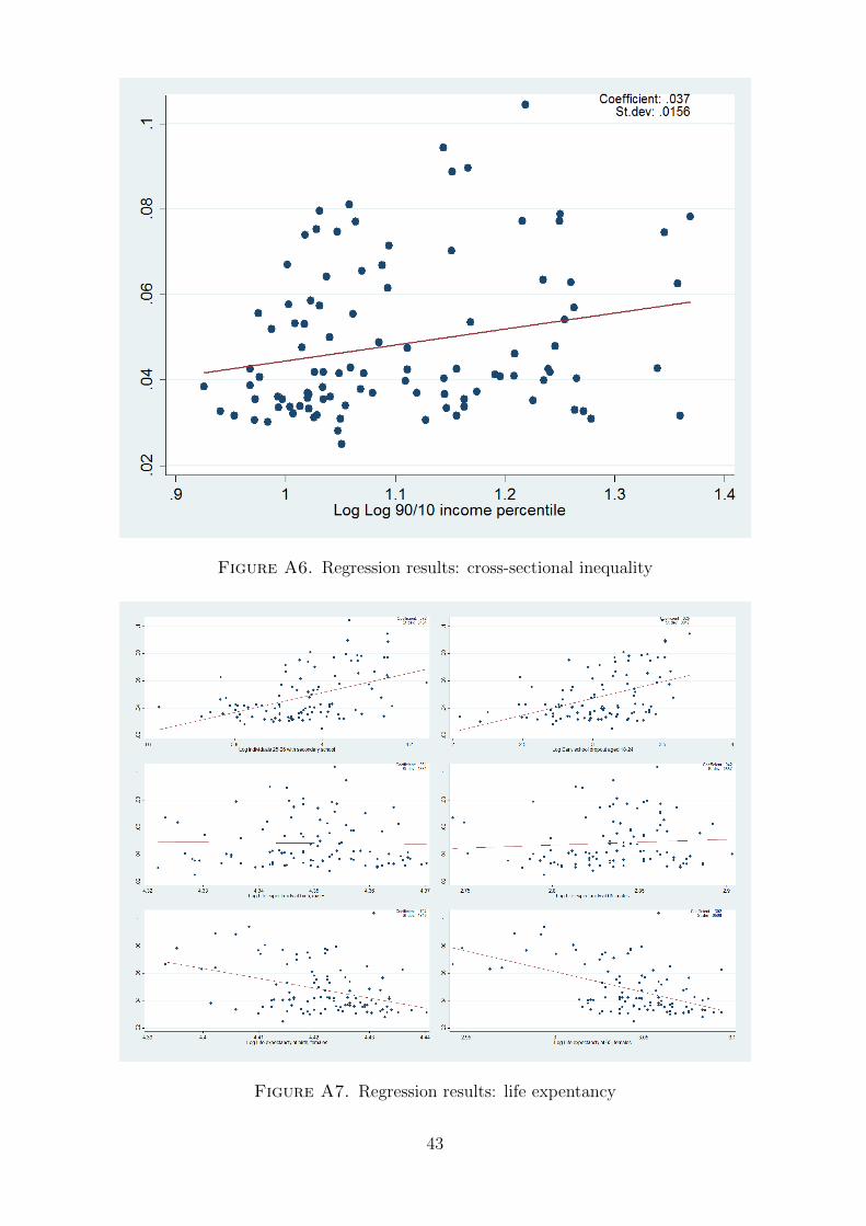
Figure A6. Regression results: cross-sectional inequality
Figure A7. Regression results: life expentancy
43

Figure A8. Regression results: suicides
Figure A9. Regression results: crime
44

Figure A10. Regression results: social capital
Figure A11. Regression results: public sector activity
45