CORRECTOR ESTIMATES FOR HIGHER-ORDER

LINEARIZATIONS IN STOCHASTIC HOMOGENIZATION OF

NONLINEAR UNIFORMLY ELLIPTIC EQUATIONS

SEBASTIAN HENSEL

Abstract. Corrector estimates constitute a key ingredient in the derivationof optimal convergence rates via two-scale expansion techniques in homog-

enization theory of random uniformly elliptic equations. The present work

follows up—in terms of corrector estimates—on the recent work of Fischerand Neukamm (arXiv:1908.02273) which provides a quantitative stochastic

homogenization theory of nonlinear uniformly elliptic equations under a spec-

tral gap assumption. We establish optimal-order estimates (with respect tothe scaling in the ratio between the microscopic and the macroscopic scale)

for higher-order linearized correctors. A rather straightforward consequence of

the corrector estimates is the higher-order regularity of the associated homog-enized monotone operator.

1. Introduction

Consider the setting of a monotone, uniformly elliptic and bounded PDE

−∇ ·A(xε,∇uε

)= ∇ · f in Rd, f ∈ C∞cpt(Rd;Rd), (1)

with ε 1 denoting a microscale. We in addition assume that the monotone non-linearity A is random (see Subsection 1.4 for a precise account on the assumptionsof this work). The theory of nonlinear stochastic homogenization is then concernedwith the behavior of the solutions to equation (1) in the limit ε→ 0.

If the monotone nonlinearity is sampled according to a stationary and ergodicprobability distribution (which we will always assume), the classical qualitativeprediction (see, e.g., [12] and [13]) consists of the convergence of uε to the solutionuhom of an effective nonlinear PDE

−∇ ·Ahom(∇uhom) = ∇ · f in Rd, (2)

with Ahom being a monotone, uniformly elliptic and bounded operator. In the rig-orous transition from the random model (1) to the deterministic effective model (2),next to the purely qualitative questions of convergence or the derivation of a ho-mogenization formula for the effective operator Ahom, also quantitative aspects likethe validity of convergence rates are obviously of interest.

For all of these questions in homogenization theory, the probably most fundamen-tal concept is the notion of the homogenization corrector φεξ, which for a constant

macroscopic field gradient ξ ∈ Rd is given by the almost surely sublinearly growingsolution of

−∇ ·A(xε, ξ+∇φεξ

)= 0 in Rd. (3)

1

2 SEBASTIAN HENSEL

For instance, by means of the homogenization correctors the homogenization for-mula for the effective operator reads as

Ahom(ξ) =⟨A(xε, ξ+∇φεξ

)⟩, (4)

which is well-defined as a consequence of stationarity of the underlying probabilitydistribution. For quantitatively inclined questions like those concerned with thederivation of convergence rates, it is useful to introduce in addition a notion of fluxcorrectors. For a given constant macroscopic field gradient ξ ∈ Rd, the associatedflux corrector σξ is a random field with almost surely sublinear growth at infinity,

taking values in the skew-symmetric matrices Rd×dskew, and solving

∇ · σεξ = A(xε, ξ+∇φεξ

)−Ahom(ξ) in Rd. (5)

The merit of the corrector pair (φεξ, σεξ) is that it allows to represent, at least on a

formal level, the error for the two-scale expansion wε := uhom(x)+φεξ(x)|ξ=∇uhom(x)

in divergence form by means of first-order linearized correctors

−∇ ·A(xε,∇wε

)= ∇ · f −∇ ·

(((aεξ ⊗ ∂ξφεξ)|ξ=∇uhom(x)−∂ξσεξ |ξ=∇uhom(x)

): ∇2uhom

),

(6)

where we also introduced the linearized coefficient field aεξ := (∂ξA)(xε , ξ+∇φεξ). It is

clear from the previous display that estimates on the corrector pair (φεξ, σεξ) (and its

first-order linearization) constitute a key ingredient in quantifying the convergenceuε → uhom. In the present nonlinear setting, we refer to the recent work of Fischerand Neukamm [18] where this program was carried out in the regime of a spectralgap assumption, resulting in homogenization error estimates being optimal in termsof scaling with respect to ε.

We establish in the present work optimal-order estimates (with respect to thescaling in ε) for higher-order linearized homogenization and flux correctors. Givena linearization order L ∈ N0 and a family of vectors w1, . . . , wL ∈ Rd, the Lth or-der linearized homogenization corrector is formally given by the directional deriva-tive φεξ,w1···wL = (∂ξφ

εξ)[w1· · ·wL]. Its defining PDE may be obtained by dif-

ferentiating the nonlinear corrector problem (3) in the macroscopic variable ξ ∈ Rd.In particular, note that φεξ,w1···wL = εφξ,w1···wL( ·ε ) where φξ,w1···wL for-

mally represents the Lth order directional derivative (in direction of w1· · ·wL)of the almost surely sublinearly growing solution of

−∇ ·A(x, ξ+∇φξ) = 0 in Rd. (7)

We then derive on the level of φξ,w1···wL , amongst other things (cf. Theorem 1for a more precise statement), corrector estimates of the form⟨∣∣∣∣−ˆ

B1(x0)

∣∣φξ,w1···wL∣∣2∣∣∣∣q⟩ 1

q

.L,q,|ξ| |w1|2 · · · |wL|2µ2∗(1+|x0|

)(8)

with the scaling function µ∗ : R>0 → R>0 defined by (20). This in turn implies⟨∣∣∣∣−ˆBε(x0)

∣∣φεξ,w1···wL

∣∣2∣∣∣∣q⟩ 1q

.L,q,|ξ| ε2µ2∗

(1

ε

)|w1|2 · · · |wL|2µ2

∗(1+|x0|

)(9)

HIGHER-ORDER LINEARIZED CORRECTORS IN STOCHASTIC HOMOGENIZATION 3

as is immediate from the scaling relation φεξ,w1···wL = εφξ,w1···wL( ·ε ), a change

of variables as well as (20). In the case L = 1, this recovers the optimal-ordercorrector estimates of [18]. As properties of φξ,w1···wL may always be translatedinto properties of φεξ,w1···wL based on their scaling relation, from Section 1.4

onwards we set ε = 1 and study higher-order linearizations of (7).For a proof of corrector estimates of the form (8) in terms of higher-order lin-

earized correctors, we devise a suitable inductive scheme to propagate corrector es-timates from one linearization order to the next. The actual implementation of thisinductive scheme, cf. Subsections 3.4–3.7 below, is in large parts directly inspiredby the methods of Gloria, Neukamm and Otto [22]–[21], Fischer and Neukamm [18]as well as Josien and Otto [29]. Similar to the latter two works, we also employ asmall-scale regularity assumption (see Assumption 3 below).

1.1. Applications for corrector estimates of higher-order linearizations.The motivation for the present work derives from the expectation that estimatesfor higher-order linearized correctors constitute one of the important ingredients foropen questions of interest in nonlinear stochastic homogenization, e.g., i) an optimalquantification of the commutability of homogenization and linearization (cf. [2]and [1] for suboptimal algebraic rates in the regime of finite range of dependence),or ii) the development of a nonlinear analogue of the theory of fluctuations asworked out for the linear case in [16], [15] and [14].

The former for instance concerns the study of the homogenization of the first-order linearized problem

−∇ · (∂ξA)(xε,∇uε

)∇U (1)

ε = ∇ · f (1) in Rd, f (1) ∈ C∞cpt(Rd;Rd) (10)

towards the linearized effective equation

−∇ · (∂ξAhom)(∇uhom)∇U (1)hom = ∇ · f (1) in Rd; (11)

of course under appropriate regularity assumption for the nonlinearity. It is natural

to define a two-scale expansion of U(1)ε in terms of first-order linearized homoge-

nization correctors W(1)ε := U

(1)hom + (∂ξφ

εξ)[∇U

(1)hom]

∣∣ξ=∇uhom

, so that the differ-

ence ∇U (1)ε −∇W (1)

ε formally satisfies a uniformly elliptic equation with fluctuatingcoefficient (∂ξA)(xε ,∇uε) and a right hand side, which—amongst other terms—inparticular features second-order linearized homogenization (and flux) correctors.The estimates obtained in the present work therefore represent a key ingredient ifone aims for a derivation of optimal-order convergence rates of the homogenizationof (10) towards (11).

The second topic mentioned above concerns the study of the random fluctuationsof several macroscopic observables of interest in homogenization theory, e.g.,ˆ

RdF · ∇uε,

ˆRdF · ∇φεξ, F ∈ C∞cpt(Rd;Rd). (12)

In the works [16] and [15], Duerinckx, Gloria and Otto identified in the frameworkof linear stochastic homogenization A(·, ξ) = a(·)ξ an object, the so-called standardhomogenization corrector

Ξξ := (a−ahom)(ξ+∇φξ), (13)

which relates the fluctuations of the corrector gradients with the fluctuations of thefield ∇uε. That fluctuations are related in terms of a single object is by no means

4 SEBASTIAN HENSEL

obvious as substituting naively a two-scale expansion for ∇uε in´Rd F · ∇uε does

not characterize the fluctuations of´Rd F ·∇uε to leading order as observed in [27].

In a forthcoming work [28], we perform an intermediate step towards understand-ing the fluctuations of random variables of the form (12) in nonlinear settings. Tothis end, we introduce a nonlinear counterpart of the standard homogenizationcommutator (13) and derive a scaling limit result in a Gaussian setting (cf. [14]).As in the linear regime, this nonlinear counterpart of (13) also dictates the fluctu-ations of linear functionals of the corrector gradients ∇φξ (and their (higher-order)linearized descendants in terms of (higher-order) linearized homogenization commu-tators). The results of the work [28] are based, amongst other things, on estimatesfor higher-order linearized homogenization and flux correctors of the dual linearizedoperator −∇ · a∗ξ∇ (cf. Section 2.4 below), where a∗ξ denotes the transpose of the

linearized coefficient field aξ := (∂ξA)(ω, ξ+∇φξ).

1.2. Stochastic homogenization of linear uniformly elliptic equations andsystems. Before we give a precise account of the underlying assumptions for thepresent work in Subsection 1.4, let us first briefly review the by-now substantialliterature on the subject. The classical results in qualitative stochastic homoge-nization are due to Papanicolaou and Varadhan [37] and Kozlov [30], who studiedheat conduction in a randomly heterogeneous medium under the assumption ofstationarity and ergodicity (for the discrete setting, see [31] and [32]). The first re-sult in quantitative stochastic homogenization is due to Yurinskii [39], who deriveda suboptimal quantitative result for linear elliptic PDEs under a uniform mixingcondition. Naddaf and Spencer [36] expressed mixing for the first time in the formof a spectral gap inequality, and as a result obtained optimal results for the fluctua-tions of the energy density of the corrector. Their work is however limited to smallellipticity contrast, see also Conlon and Naddaf [10] or Conlon and Fahim [11].

Extensions to the non-perturbative regime in the discrete setting were estab-lished through a series of articles by Gloria and Otto [23], [24] and [26], see alsoGloria, Neukamm and Otto [20]. These works contain optimal estimates for theapproximation error of the homogenized coefficients, the approximation error forthe solutions, the corrector as well as the fluctuation of the energy density of thecorrector under the assumption of i.i.d. conductivities. In the continuum settingand under spectral gap type assumptions, we refer to the works [22] and [21] ofGloria, Neukamm and Otto for optimal-order estimates in linear stochastic homog-enization. Armstrong, Mourrat and Kuusi [3] establish these results in the finiterange of dependence regime including also optimal stochastic integrability, see tothis end also Gloria and Otto [25].

1.3. Stochastic homogenization in nonlinear settings. In the context of qual-itative nonlinear stochastic homogenization, the first results are due to Dal Masoand Modica [12] and [13] in the setting of convex integral functionals. Lions andSouganidis [33] studied the homogenization of Hamilton–Jacobi equations under thequalitative assumptions of stationarity and ergodicity. Caffarelli, Souganidis andWang [9] obtained stochastic homogenization in the context of nonlinear, uniformlyelliptic equations in divergence form (see also Armstrong and Smart [5]). A homog-enization result in the same framework but without assuming uniform ellipticity isdue to Armstrong and Smart [6]. For an example of stochastic homogenization fornonlinear nonlocal equations, we refer to Schwab [38].

HIGHER-ORDER LINEARIZED CORRECTORS IN STOCHASTIC HOMOGENIZATION 5

A first quantitative result in the context of nonlinear stochastic homogenizationwas established by Caffarelli and Souganidis [8], who succeeded in the derivationof a logarithmic-type convergence rate under strong mixing conditions. Substantialprogress in the nonlinear setting was later provided by the works of Armstrongand Smart [7] on uniformly convex integral functionals, and Armstrong and Mour-rat [4] on elliptic equations in divergence form with monotone coefficient fields. Inthe two recent works [2] resp. [1], Armstrong, Ferguson and Kuusi succeeded inproving that the processes of homogenization and (first-order resp. higher-order)linearization commute. Moreover, as it is also the case in the previously mentionedworks of Armstrong et al., they derive quantitative estimates in terms of a subop-timal algebraic rate of convergence with respect to the ratio in the microscopic andmacroscopic scale, assuming finite range of dependence for the underlying proba-bility space. The established estimates, however, are optimal in terms of stochasticintegrability. Under a spectral gap assumption, Fischer and Neukamm [18] recentlyprovided quantitative homogenization estimates for monotone uniformly elliptic co-efficient fields, which on one side are the first being optimal in the ratio betweenthe microscopic and macroscopic scale, but which on the other side are non-optimalin terms of stochastic integrability.

1.4. Assumptions and setting. In this section, we give a precise account of theunderlying assumptions for the present work. They represent the natural higher-order analogues of the assumptions from [18]. We start with the deterministicrequirements on the family of monotone operators (cf. [18, Section 2.1]).

Assumption 1 (Family of monotone operators). Let d ∈ N be the spatial dimen-sion, and let 0 < λ ≤ Λ < ∞ be two constants (playing the role of ellipticityconstants in the sequel). Let n ∈ N and L ∈ N0 be given. We then assume that weare equipped with a family of operators indexed by elements of Rn

A : Rn × Rd → Rd

which is subject to the following three conditions:

(A1) The map A gives rise to a family of monotone operators in the secondvariable with lower bound λ. More precisely, for all ω ∈ Rn we require(

A(ω, ξ1)−A(ω, ξ2))· (ξ1−ξ2) ≥ λ|ξ1−ξ2|2

for all ξ1, ξ2 ∈ Rd. Furthermore, A(ω, 0) = 0 for all ω ∈ Rn.(A2)L Each operator A(ω, ·), ω ∈ Rn, is L+1 times continuously differentiable in

the second variable. In quantitative terms, we assume that for all ω ∈ Rn

supk∈1,...,L+1

supξ∈Rd

∣∣(∂kξA)(ω, ξ)∣∣ ≤ Λ,

supk∈1,...,L+1

supξ∈Rd

supω1,ω2∈Rn, ω1 6=ω2

|(∂kξA)(ω1, ξ)− (∂kξA)(ω2, ξ)||ω1 − ω2|

≤ Λ.

In particular, we have |A(ω, ξ)| ≤ Λ|ξ| for all ω ∈ Rn and all ξ ∈ Rd.(A3)L For each ξ ∈ Rd and k ∈ 0, . . . , L, the map ω 7→ (∂kξA)(ω, ξ) is differen-

tiable with uniformly Lipschitz continuous derivative. In quantitative terms,

6 SEBASTIAN HENSEL

the following bounds are required to hold true for all ω ∈ Rn and all ξ ∈ Rd

|(∂ωA)(ω, ξ)| ≤ Λ|ξ|, supk∈1,...,L

|(∂ω∂kξA)(ω, ξ)| ≤ Λ,

supω1,ω2∈Rn, ω1 6=ω2

|(∂ωA)(ω1, ξ)− (∂ωA)(ω2, ξ)||ω1 − ω2|

≤ Λ|ξ|,

supk∈1,...,L

supω1,ω2∈Rn, ω1 6=ω2

|(∂ω∂kξA)(ω1, ξ)− (∂ω∂kξA)(ω2, ξ)|

|ω1 − ω2|≤ Λ.

For some results, we in addition require the following condition to be true.

(A4)L For each ω ∈ Rn, the maps ξ 7→ (∂L+1ξ A)(ω, ξ) and ξ 7→ (∂ω∂

Lξ A)(ω, ξ)

are uniformly Lipschitz continuous. More precisely, for all ω ∈ Rn we areequipped with bounds

supξ1,ξ2∈Rd, ξ1 6=ξ2

|(∂L+1ξ A)(ω, ξ1)− (∂L+1

ξ A)(ω, ξ2)||ξ1 − ξ2|

≤ Λ.

supξ1,ξ2∈Rd, ξ1 6=ξ2

|(∂ω∂Lξ A)(ω, ξ1)− (∂ω∂Lξ A)(ω, ξ2)|

|ξ1 − ξ2|≤ Λ.

Having the deterministic requirements on the family of monotone operators inplace, we next turn to the probabilistic assumptions.

Assumption 2 (Stationarity and quantified ergodicity for probability distribu-tion of parameter fields). We call a measurable function ω : Rd → Rn a parameterfield, and denote by Ω the space of parameter fields with the L1

loc(Rd;Rn) topol-ogy. We assume that we are equipped with a probability measure P on Ω so thatP[ω : [ω]Cη(B1(x0)) < ∞ for all x0 ∈ Rd] = 1 for some η ∈ (0, 1), and which issubject to the following two further conditions:

(P1) The probability measure P on Ω is Rd-stationary. In other words, the prob-ability distributions of ω(·) and ω(·+ z) coincide for all shifts z ∈ Rd.

(P2) The probability measure P on Ω is ergodic. We in fact require a strongercondition in form of a spectral gap inequality as follows: Denoting with 〈·〉the expectation with respect to P, there exists a constant Csg > 0 such

that for all random variables X ∈⋂q≥1 L

2q〈·〉 for which there exists ∂fctX

satisfying [∂fctX]1 ∈⋂q≥1 L

2q〈·〉L

2(Rd;Rn) as well as

limt↓0

X(ω+tδω)−X(ω)

t=

ˆδω · ∂fctX in

⋂q≥1

L2q〈·〉 (14)

for all perturbations δω ∈ Cηuloc(Rd;Rn) with ‖[δω]∞‖L2(Rd) < ∞, we thenhave the estimate⟨∣∣X−〈X〉∣∣2⟩ ≤ C2

sg

⟨ˆ (−ˆB1(x)

∣∣∂fctX∣∣ )2⟩

. (15)

We finally require a stronger form of the already stated small-scale regularity as-sumption P[ω : [ω]Cη(B1(x0)) <∞ for all x0 ∈ Rd] = 1, which in turn is essentialto obtain optimal-order estimates (i.e., with respect to the ratio of the microscopicand macroscopic scale) for linearized homogenization and flux correctors, as wellas their higher-order analogues.

HIGHER-ORDER LINEARIZED CORRECTORS IN STOCHASTIC HOMOGENIZATION 7

Assumption 3 (Annealed small-scale regularity condition). Let the conditions andnotation of Assumption 2 be in place; in particular, let η ∈ (0, 1) be the associatedHolder continuity exponent. We then in addition require that

(R) There exist constants Creg, C′reg > 0 such that for all q ∈ [1,∞) it holds⟨∣∣∣∣ sup

x,y∈B1, x 6=y

|ω(x)− ω(y)||x− y|η

∣∣∣∣2q⟩ 1q

≤ C2regq

2C′reg .

Note that our small-scale regularity condition is slightly weaker than the corre-sponding assumption in [18]. For this reason we provide a proof in Appendix Aconcerning the small-scale Holder regularity of the (massive) corrector solving thenonlinear corrector problem (44a), see Lemma 23, which in turn implies small-scaleHolder regularity of the linearized coefficient field, see Lemma 24.

1.5. Example. We give an example for a random parameter field subject to As-sumption 2 and Assumption 3. To this end, consider first a (for notational con-venience 1-dimensional) white noise W : L2(Rd) → L2(Ω,F ,P) constructed oversome probability space (Ω,F ,P). (We may assume without loss of generality thatthe σ-algebra F is the one generated by W (h), h ∈ L2(Rd).) In other words,(W (h))h∈L2(Rd) is a family of centered, real-valued Gaussian random variables such

that 〈W (h)W (g)〉 =´hg.

Given some c0 ∈ L2(Rd) satisfying the following decay assumption on its (non-negative) Fourier transform c0 for some α ∈ (0, 1)

0 ≤ c0(k) ≤ C(1+|k|)−d+2α

2 , k ∈ Rd,

we then define a stationary and centered Gaussian random field with boundedcovariance function c := c0 ∗ c−0 : Rd → R, c−0 (x) := c0(−x), by means of

ω(x) := (c0 ∗W )(x) := W(c0(x−·)

).

Since the decay of c0 translates into 0 ≤ c(k) = c0(k)c0(−k) ≤ C(1+|k|)−(d−2α), itis a well-known fact that, for any η ∈ (0, α), the Gaussian random field is η-Holdercontinuous with probability one. In fact, one can show that Assumption 3 holdstrue. For a proof, see, e.g., [29, Lemma 3.1, Appendix A.3.1].

Moreover, the spectral gap inequality (15) is a consequence of Malliavin calculusassociated with the underlying white noise W which can be seen as follows. Fix asquare integrable h ∈ L2(Rd), and define δω := c0 ∗ h. We haveˆ

supy∈B1(x)

(δω)2(y) .ˆ

(1+|k|)d+2α|δω|2 dk .ˆ|h|2 dk <∞,

where the first inequality is a consequence of a Sobolev embedding (see, e.g., [29,

Appendix A.2]), whereas the second follows from δω = c0 h together with the decayassumption on c0. Furthermore, for any x, y ∈ Rd with x 6= y we may estimate

|δω(x)−δω(y)| ≤ˆ ∣∣eikx−eiky∣∣∣∣c0(−k)

∣∣∣∣h∣∣dk . ( ˆ (1 ∧ |k(x−y)|2)∣∣c0(−k)

∣∣2 dk

) 12

. |x−y|α(ˆ

(1 ∧ |k|2)|k|−d−2α dk

) 12

. |x−y|α.

8 SEBASTIAN HENSEL

Hence, δω = c0 ∗ h is an admissible test function for the condition of (14) for all

h ∈ L2(Rd). In other words, for any random variable X ∈⋂q≥1 L

2q〈·〉 satisfying (14)

one recognizes the field c−0 ∗ ∂fctX as its Malliavin derivative DX (since the fieldsc0 ∗ h, h ∈ L2(Rd), represent precisely the elements of the Cameron–Martin spaceassociated with the Gaussian measure on L1

loc(Rd) induced by the Gaussian randomfield ω; cf. [34] for Malliavin calculus), which then also satisfies the estimate

〈‖DX‖2L2(Rd)〉 .⟨ˆ

(1+|k|)−d−2α|∂fctX|2 dk

⟩.⟨∥∥[∂fctX]1

∥∥2

L2(Rd)

⟩.

We thus arrived at the right hand side of (15). That the left hand side from the

previous display is bounded from below by⟨∣∣X−〈X〉∣∣2⟩ is finally nothing else but

the well-known first-order Poincare inequality on probability space (see, e.g., [17,Proposition 4.1, Appendix A]).

1.6. Notation. We denote by N the set of positive integers, and define N0 :=N∪0. For given d ∈ N, the space of real-valued d×d matrices is denoted by Rd×d.The transpose of a matrix A ∈ Rd×d is given by A∗. We write Rd×dskew for the spaceof skew-symmetric matrices A∗ = −A. For a given L ∈ N, we define Par1, . . . , Lto be the set of all partitions of 1, . . . , L. For any x0 ∈ Rd and R > 0, we denoteby BR(x0) ⊂ Rd the d-dimensional open ball of radius R centered at x0. In case ofx0 = 0, we simply write BR. In the rare occasion that the dimension of the ambientspace is not represented by d ∈ N but, say, n ∈ N, we emphasize the dimensionof the ambient space by writing BnR(x0) for the n-dimensional open ball of radiusR > 0 centered at x0 ∈ Rn.

The tensor product of vectors v1, . . . , vL ∈ Rd, L ≥ 2, is denoted by v1⊗· · ·⊗vL.For the symmetric tensor product, we write v1· · ·vL. The L-fold tensor productof a vector v ∈ Rd is abbreviated as v⊗L; or vL for the corresponding symmetricversion. For a differentiable map A : Rn×Rd → Rd, (ω, ξ) 7→ A(ω, ξ), we make useof the usual notation ∂ωA, ∂ξA for the respective partial derivatives. Higher-order(possibly mixed) partial derivatives of a map A : Rn × Rd → Rd are denoted by∂lωA, ∂

kξA, ∂

lω∂

kξA for any k, l ∈ N.

Integrals´Rd f dx with respect to the d-dimensional Lebesgue measure are ab-

breviated in the course of the paper as´f . Given a Lebesgue-measurable subset

A ⊂ Rd with finite and non-trivial Lebesgue measure |A| ∈ (0,∞), we denote by−Af := 1

|A|´1Af the average integral of f over A. Here, 1A represents the charac-

teristic function with respect to a set A. For a probability measure P on a measurespace (Ω,A), we write 〈·〉 for the expectation with respect to P.

We make use of the usual notation of Lebesgue and Sobolev spaces on Rd (withrespect to the Lebesgue measure), e.g., Lp(Rd), W 1,p(Rd), H1(Rd) := W 1,2(Rd)and so on. For a probability measure P on a measure space (Ω,A), we instead usethe notation Lp〈·〉. If we want to emphasize the target space, say, a finite-dimensional

real vector space V , we do so by writing Lp(Rd;V ). For the Lebesgue resp. Sobolevspaces on Rd with only locally finite norm, we write Lploc(Rd), H1

loc(Rd) and so on.Furthermore, in the case of uniformly locally finite norm, i.e.,

supx0∈Rd

‖f‖Lp(B1(x0)) <∞ resp. supx0∈Rd

‖f‖H1(B1(x0)) <∞

we reserve the notation Lpuloc(Rd) resp. H1uloc(Rd) for the corresponding subspaces of

Lploc(Rd) resp.H1loc(Rd). The subspace of locally p-integrable functions f ∈ Lploc(Rd)

HIGHER-ORDER LINEARIZED CORRECTORS IN STOCHASTIC HOMOGENIZATION 9

satisfying

supx0∈Rd

lim supR→∞

−ˆBR(x0)

|f |p dx <∞

is in turn denoted by Lperg(Rd). Local Lp averages (with the obvious modification

for p =∞) will also be abbreviated as [f ]p(x) := ( −B1(x)

|f |p)1p .

The space of all compactly supported and smooth functions on Rd is denotedby C∞cpt(Rd). For η ∈ (0, 1) and x0 ∈ Rd, we further define the local Holder semi-

norm [f ]Cη(B1(x0)) := supx,y∈B1(x0),x 6=y|f(x)−f(y)||x−y|η and the norm ‖f‖Cη(B1(x0)) :=

‖f‖L∞(B1(x0)) +[f ]Cη(B1(x0)). We say f ∈ Cηuloc(Rd) if supx0∈Rd ‖f‖Cη(B1(x0)) <∞.Finally, for an exponent q ∈ [1,∞], we write q∗ ∈ [1,∞] for its dual Holder expo-nent: 1

q + 1q∗

= 1.

1.7. Structure of the paper. In the upcoming Section 2, we formulate the mainresults of the present work and provide definitions for the underlying key objects.Section 3 is devoted to a discussion of the strategy for the proof of the main results.In the course of it, we also collect several auxiliary results representing the mainsteps in the proof. Section 4 contains the proofs of all the main and auxiliary resultsas stated in the previous two sections. The paper finishes with three appendices. InAppendix A we list (and partly prove) several results from elliptic regularity theory.Most of them are classical results from deterministic theory. In addition, we alsorely on some annealed regularity theory; however, only in a perturbative regime a laMeyers. Appendix B deals with existence of higher-order linearized correctors for asuitable class of parameter fields. Finally, as the proof of the main results proceedsby an induction over the linearization order, we formulate and prove in Appendix Cthe corresponding statements taking care of the base case of the induction.

2. Main results

This section collects the statements of the main results of this work which aretwofold: i) corrector estimates for higher-order linearizations of the nonlinear prob-lem, and ii) higher-order regularity of the homogenized monotone operator.

2.1. Corrector bounds for higher-order linearized correctors. The firstmain result constitutes the analogue (and slight extension) of [18, Corollary 15]for the higher-order linearized correctors of Definition 4.

Theorem 1 (Corrector estimates for higher-order linearizations). Let L ∈ N andM > 0 be fixed. Let the requirements and notation of (A1), (A2)L and (A3)L ofAssumption 1, (P1) and (P2) of Assumption 2, and (R) of Assumption 3 be inplace. Fix a set of vectors w1, . . . , wL ∈ Rd and define B := w1 · · · wL. Let

φξ,B ∈ H1loc(Rd) and σξ,B ∈ H1

loc(Rd;Rd×dskew)

be the linearized homogenization and flux corrector from Definition 4.There exist C = C(d, λ,Λ, Csg, Creg, η,M,L), C ′ = C ′(d, λ,Λ, C ′reg, η, L) and

α = α(d, λ,Λ) ∈ (0, η) such that for all |ξ| ≤ M , all q ∈ [1,∞), all x0 ∈ Rd, and

10 SEBASTIAN HENSEL

all compactly supported and square-integrable deterministic fields gφ, gσ it holds⟨∣∣∣∣(ˆ gφ · ∇φξ,B ,ˆgklσ · ∇σξ,B,kl

)∣∣∣∣2q⟩ 1q

≤ C2q2C′ |B|2ˆ ∣∣(gφ, gσ)∣∣2, (16)⟨∥∥(∇φξ,B ,∇σξ,B)∥∥2q

L2(B1)

⟩ 1q ≤ C2q2C′ |B|2, (17)⟨∥∥(∇φξ,B ,∇σξ,B)∥∥2q

Cα(B1)

⟩ 1q ≤ C2q2C′ |B|2, (18)⟨∣∣∣∣−ˆ

B1(x0)

∣∣(φξ,B , σξ,B)∣∣2∣∣∣∣q⟩ 1q

≤ C2q2C′ |B|2µ2∗(1+|x0|

), (19)

with the scaling function µ∗ : R>0 → R>0 defined by

µ∗(`) :=

`

12 , d = 1,

log12 (1+`), d = 2,

1, d ≥ 3.

(20)

Let ξ0 ∈ Rd and K ∈ N0 be fixed, and assume in addition to the previous re-quirements that (A2)L+K and (A3)L+K from Assumption 1 hold true. We maythen define P-almost surely Kth-order Taylor expansions for the linearized homog-enization and flux correctors with base point ξ0 by means of

ΦKξ0,B(ξ) := φξ,B −K∑k=0

1

k!(∂ξφξ0,B)

[(ξ−ξ0)k

]∈ H1

loc(Rd), (21)

ΣKξ0,B(ξ) := σξ,B −K∑k=0

1

k!(∂ξσξ0,B)

[(ξ−ξ0)k

]∈ H1

loc(Rd;Rd×dskew). (22)

Under the stronger assumptions of (A2)L+K+1 and (A3)L+K+1 from Assumption 1,there exist constants C = C(d, λ,Λ, Csg, Creg, η,M,L,K), C ′ = C ′(d, λ,Λ, C ′reg, η, L)and α = α(d, λ,Λ) ∈ (0, η) such that for all |(ξ0, ξ)| ≤ M , all q ∈ [1,∞), and allx0 ∈ Rd it holds⟨∥∥(∇ΦKξ0,B(ξ),∇ΣKξ0,B(ξ)

)∥∥2q

L2(B1)

⟩ 1q ≤ C2q2C′ |B|2|ξ−ξ0|2(K+1), (23)⟨∥∥(∇ΦKξ0,B(ξ),∇ΣKξ0,B(ξ)

)∥∥2q

Cα(B1)

⟩ 1q ≤ C2q2C′ |B|2|ξ−ξ0|2(K+1), (24)⟨∣∣∣∣−ˆ

B1(x0)

∣∣(ΦKξ0,B(ξ),ΣKξ0,B(ξ))∣∣2∣∣∣∣q⟩ 1

q

≤ C2q2C′ |B|2|ξ−ξ0|2(K+1)µ2∗(1+|x0|

). (25)

2.2. Differentiability of the homogenized operator. A rather straightforwardconsequence of the estimates for higher-order linearized correctors is the higher-order regularity of the associated homogenized monotone operator.

Theorem 2 (Higher-order regularity of the homogenized operator). Let L ∈ Nand M > 0 be fixed. Let the requirements and notation of (A1), (A2)L and (A3)Lof Assumption 1, (P1) and (P2) of Assumption 2, and (R) of Assumption 3 be inplace. Fix next a set of vectors w1, . . . , wL ∈ Rd and define B := w1 · · · wL.Let finally

Rd 3 ξ 7→ A(ξ) := 〈qξ〉 (26)

be the homogenized operator, with the flux qξ being defined in (29b).

HIGHER-ORDER LINEARIZED CORRECTORS IN STOCHASTIC HOMOGENIZATION 11

The homogenized operator is L times differentiable as a map ξ 7→ A(ξ). Thereexists a constant C = C(d, λ,Λ, Csg, Creg, C

′reg, η,M,L) such that for all |ξ| ≤ M

its Lth Gateaux derivative in direction B admits the bound∣∣(∂Lξ A)(ξ)[B]∣∣ ≤ C|B|. (27)

Finally, we have the following representation for the Lth order Gateaux derivativein direction B

(∂Lξ A)(ξ)[B] = 〈qξ,B〉. (28)

Here, qξ,B denotes the linearized flux from (30b).

2.3. Basic definitions. We introduce the precise definitions of the homogeniza-tion and flux correctors and their (higher-order) linearized analogues. We start byrecalling these notions on the level of the nonlinear problem.

Given ξ ∈ Rd, the equation for the homogenization corrector is given by

−∇ ·A(ω, ξ+∇φξ) = 0. (29a)

Abbreviating the flux by means of

qξ := A(ω, ξ+∇φξ), (29b)

the equation for the corresponding flux corrector is given by

−∆σξ,kl = (el ⊗ ek − ek ⊗ el) : ∇qξ. (29c)

Sublinear growth of the flux corrector gives rise to

qξ − 〈qξ〉 = ∇ · σξ. (29d)

Definition 3 (Homogenization correctors and flux correctors of the nonlinear prob-lem). Let the requirements and notation of (A1), (A2)0 and (A3)0 of Assumption 1,as well as (P1) and (P2) of Assumption 2 be in place. Let ξ ∈ Rd be given. Thecorresponding homogenization corrector φξ and flux corrector σξ are two randomfields

(φξ, σξ) : Ω× Rd → R× Rd×dskew

subject to the following list of requirements:

(i) It holds P-almost surely that φξ ∈ H1loc(Rd), σξ ∈ H1

loc(Rd;Rd×dskew) as well as−B1

(φξ, σξ) dx = 0. In addition, the associated PDEs (29a) resp. (29c) and (29d)

are satisfied in the distributional sense P-almost surely.(ii) The gradients ∇φξ and ∇σξ are stationary random fields. Moreover, it holds⟨

(∇φξ,∇σξ)⟩

= 0,⟨|∇φξ|2

⟩+⟨|∇σξ|2

⟩<∞.

(iii) The two random fields φξ and σξ feature P-almost surely sublinear growth atinfinity

limR→∞

1

R2−ˆBR

∣∣(φξ, σξ)∣∣2 dx = 0.

We next introduce the (higher-order) linearized analogues of the corrector equa-tions (29a)–(29d) by formally differentiating in the macroscopic variable. To thisend, let a linearization order L ∈ N be fixed. We also fix vectors w1, . . . , wL ∈ Rdand let B := w1 · · · wL. Finally, fix ξ ∈ Rd and denote by aξ the coefficientfield (∂ξA)(ω, ξ+∇φξ). Due to (A1) and (A2)0 from Assumption 1, this coefficient

12 SEBASTIAN HENSEL

field is uniformly elliptic and bounded with respect to the same constants (λ,Λ)from Assumption 1.

As suggested by the Faa di Bruno formula, the equation for the Lth-order lin-earized homogenization corrector in direction B shall be given by

−∇ · aξ(1L=1B +∇φξ,B)

= ∇ ·∑

Π∈Par1,...,LΠ6=1,...,L

(∂|Π|ξ A)(ω, ξ+∇φξ)

[⊙π∈Π

(1|π|=1B′π +∇φξ,B′π )

], (30a)

where we also introduced the notational convention

B′π :=⊙m∈π

vm, ∀π ∈ Π, Π ∈ Par1, . . . , L.

Note that the right hand side only features linearized correctors of order ≤ L−1, ifany. Motivated by this observation, existence of solutions to the linearized correc-tor problem (30a) with stationary gradient and (almost sure) sublinear growth atinfinity will be given inductively through approximation with an additional mas-sive term, see (49a) for the associated corrector problem. For the latter, solutionsmay be constructed—again inductively—on purely deterministic grounds (undersuitable assumptions which are in particular modeled on the small-scale regularitycondition (R) from Assumption 3). For more details, we refer the reader to thediscussion in Section 3.2 below.

To state the equation for the linearized flux corrector, we first define the lin-earized flux by means of

qξ,B := aξ(1L=1B +∇φξ,B)

+∑

Π∈Par1,...,LΠ6=1,...,L

(∂|Π|ξ A)(ω, ξ+∇φξ)

[⊙π∈Π

(1|π|=1B′π +∇φξ,B′π )

]. (30b)

The associated flux corrector shall then be a solution of

−∆σξ,B,kl = (el ⊗ ek − ek ⊗ el) : ∇qξ,B . (30c)

Due to the sublinear growth of the correctors, the previous relations entail that

qξ,B − 〈qξ,B〉 = ∇ · σξ,B . (30d)

Definition 4 (Higher-order linearized homogenization correctors and flux correc-tors). Let L ∈ N and ξ ∈ Rd be fixed. Let the requirements and notation of (A1),(A2)L and (A3)L of Assumption 1, (P1) and (P2) of Assumption 2, and (R) ofAssumption 3 be in place. We also fix a set of vectors w1, . . . , wL ∈ Rd and defineB := w1 · · · wL. The corresponding linearized homogenization corrector φξ,Band flux corrector σξ,B are two random fields

(φξ,B , σξ,B) : Ω× Rd → R× Rd×dskew

subject to the following list of requirements:

(i) It holds P-almost surely that φξ,B ∈ H1loc(Rd), σξ,B ∈ H1

loc(Rd;Rd×dskew) aswell as −

B1(φξ,B , σξ,B) dx = 0. In addition, the associated PDEs (30a) resp.

(30c) and (30d) are satisfied in the distributional sense P-almost surely.

HIGHER-ORDER LINEARIZED CORRECTORS IN STOCHASTIC HOMOGENIZATION 13

(ii) The gradients ∇φξ,B and ∇σξ,B are stationary random fields. Moreover, itholds ⟨

(∇φξ,B ,∇σξ,B)⟩

= 0,⟨|∇φξ,B |2

⟩+⟨|∇σξ,B |2

⟩<∞.

(iii) The two random fields φξ,B and σξ,B feature P-almost surely sublinear growthat infinity

limR→∞

1

R2−ˆBR

∣∣(φξ,B , σξ,B)∣∣2 dx = 0.

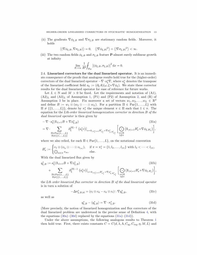
2.4. Linearized correctors for the dual linearized operator. It is an immedi-ate consequence of the proofs that analogous results hold true for the (higher-order)correctors of the dual linearized operator −∇·a∗ξ∇, where a∗ξ denotes the transpose

of the linearized coefficient field aξ := (∂ξA)(ω, ξ+∇φξ). We state these correctorresults for the dual linearized operator for ease of reference for future works.

Let L ∈ N and M > 0 be fixed. Let the requirements and notation of (A1),(A2)L and (A3)L of Assumption 1, (P1) and (P2) of Assumption 2, and (R) ofAssumption 3 be in place. Fix moreover a set of vectors w1, w2, . . . , wL ∈ Rdand define B := w1 ⊗ (w2 · · · wL). For a partition Π ∈ Par1, . . . , L withΠ 6= 1, . . . , L, denote by π∗1 the unique element π ∈ Π such that 1 ∈ π. Theequation for the Lth-order linearized homogenization corrector in direction B of thedual linearized operator is then given by

−∇ · a∗ξ(1L=1B +∇φ∗ξ,B) (31a)

= ∇ ·∑

Π∈Par1,...,LΠ6=1,...,L

∂|Π|−1ξ

(a∗ξv)∣∣v=1|π∗1 |=1B

′π∗1

+∇φ∗ξ,B′

π∗1

[⊙π∈Π1/∈π

(1|π|=1B

′π+∇φξ,B′π

)],

where we also relied, for each Π ∈ Par1, . . . , L, on the notational convention

B′π :=

v1 ⊗ (vl2 · · · vl|π|), if π = π∗1 = 1, l2, . . . , l|π| with l2 < · · · < l|π|,⊙

m∈π vm, else.

With the dual linearized flux given by

q∗ξ,B := a∗ξ(1L=1B +∇φ∗ξ,B) (31b)

+∑

Π∈Par1,...,LΠ6=1,...,L

∂|Π|−1ξ

(a∗ξv)∣∣v=1|π∗1 |=1B

′π∗1

+∇φ∗ξ,B′

π∗1

[⊙π∈Π1/∈π

(1|π|=1B

′π+∇φξ,B′π

)],

the Lth order linearized flux corrector in direction B of the dual linearized operatoris in turn a solution of

−∆σ∗ξ,B,kl = (el ⊗ ek − ek ⊗ el) : ∇q∗ξ,B , (31c)

as well as

q∗ξ,B − 〈q∗ξ,B〉 = ∇ · σ∗ξ,B . (31d)

(More precisely, the notion of linearized homogenization and flux correctors of thedual linearized problem are understood in the precise sense of Definition 4, withthe equations (30a)–(30d) replaced by the equations (31a)–(31d)).

Under the above assumptions, the following analogous results to Theorem 1then hold true. First, there exists constants C = C(d, λ,Λ, Csg, Creg, η,M,L) and

14 SEBASTIAN HENSEL

C ′ = C ′(d, λ,Λ, C ′reg, η, L) such that for all |ξ| ≤M , all q ∈ [1,∞), all x0 ∈ Rd, andall compactly supported and square-integrable gφ, gσ it holds⟨∣∣∣∣(ˆ gφ · ∇φ∗ξ,B ,

ˆgklσ · ∇σ∗ξ,B,kl

)∣∣∣∣2q⟩ 1q

≤ C2q2C′ |B|2ˆ ∣∣(gφ, gσ)∣∣2, (32)⟨∥∥(∇φ∗ξ,B ,∇σ∗ξ,B)∥∥2q

L2(B1)

⟩ 1q ≤ C2q2C′ |B|2, (33)⟨∥∥(∇φ∗ξ,B ,∇σ∗ξ,B)∥∥2q

Cα(B1)

⟩ 1q ≤ C2q2C′ |B|2, (34)⟨∣∣∣∣−ˆ

B1(x0)

∣∣(φ∗ξ,B , σ∗ξ,B)∣∣2∣∣∣∣q⟩ 1q

≤ C2q2C′ |B|2µ2∗(1+|x0|

), (35)

with the scaling function µ∗ : R>0 → R>0 defined in (20).Fix K ∈ N, and assume that (A2)L+K and (A3)L+K from Assumption 1 hold

true on top of the previous assumptions of this section. Then, both the mapsξ 7→ ∇φ∗ξ,B and ξ 7→ ∇σ∗ξ,B are P-almost surely K times Gateaux differentiable

with values in the Frechet space L2〈·〉L

2loc(Rd). Moreover, for any collection of vectors

wL+1, . . . , wL+K ∈ Rd and any k ∈ 1, . . . ,K we have the following representations

of the kth order Gateaux derivatives in direction Bk := wL+1 · · · wL+k:

(∂kξ φ∗ξ,B)[Bk] = φ∗ξ,w1⊗(w2···wL+k), (∂kξ σ

∗ξ,B)[Bk] = σ∗ξ,w1⊗(w2···wL+k). (36)

Denote by a∗ξ ∈ Rd×d the homogenized coefficient of the dual linearized operatorcharacterized by

a∗ξw = 〈q∗ξ,w〉, w ∈ Rd.

Then the following version of Theorem 2 holds true for L ≥ 1. The map ξ 7→ a∗ξis L−1 times differentiable. There exists C = C(d, λ,Λ, Csg, Creg, C

′reg, η,M,L)

such that for all |ξ| ≤ M its (L−1)th Gateaux derivative in the direction of B′ =w2 · · · wL admits the bound∣∣(∂L−1

ξ a∗ξ)[B′]

∣∣ ≤ C|B′|. (37)

We finally have for all w ∈ Rd the following representation for the (L−1)th orderGateaux derivative in direction B′(

∂L−1ξ ( a∗ξw)

)[B′] = 〈q∗ξ,w⊗B′〉. (38)

3. Outline of strategy

The proof of the corrector bounds from Theorem 1 is based on the massiveapproximation of the operator −∇ · (∂ξA)(ω, ξ + ∇φξ). For the problem with anadditional massive term, we will argue by an induction with respect to the order ofthe linearization. This will entail the following analogue of Theorem 1 in terms ofthe massive approximation.

Theorem 5 (Estimates for massive correctors). Let L ∈ N, M > 0 as well asT ∈ [1,∞) be fixed. Let the requirements and notation of (A1), (A2)L and (A3)Lof Assumption 1, (P1) and (P2) of Assumption 2, and (R) of Assumption 3 be inplace. Fix a set of unit vectors v1, . . . , vL ∈ Rd and define B := v1 · · · vL. Let

φTξ,B ∈ H1uloc(Rd), σTξ,B ∈ H1

uloc(Rd;Rd×dskew) and ψTξ,B ∈ H1uloc(Rd;Rd)

HIGHER-ORDER LINEARIZED CORRECTORS IN STOCHASTIC HOMOGENIZATION 15

denote the unique solutions of the linearized corrector problems (49a)–(49d), whichP-almost surely exist by means of Lemma 8 below.

There exist C = C(d, λ,Λ, Csg, Creg, η,M,L), C ′ = C ′(d, λ,Λ, C ′reg, η, L) andα = α(d, λ,Λ) ∈ (0, η) such that for all |ξ| ≤ M , all q ∈ [1,∞), and all compactlysupported and square-integrable fields gφ, gσ, gψ resp. fφ, fσ, fψ it holds⟨∣∣∣∣(ˆ gφ · ∇φTξ,B ,

ˆgklσ · ∇σTξ,B,kl,

ˆgkψ ·∇ψTξ,B,k√

T

)∣∣∣∣2q⟩ 1q

≤ C2q2C′ˆ ∣∣(gφ, gσ, gψ)∣∣2, (39)

and ⟨∣∣∣∣(ˆ 1

Tfφφ

Tξ,B ,

ˆ1

Tfklσ σ

Tξ,B,kl,

ˆ1

TfkψψTξ,B,k√

T

)∣∣∣∣2q⟩ 1q

≤ C2q2C′ˆ

1

T

∣∣(fφ, fσ, fψ)∣∣2, (40)

as well as ⟨∥∥∥(∇φTξ,B ,∇σTξ,B , ∇ψTξ,B√T

)∥∥∥2q

L2(B1)

⟩ 1q ≤ C2q2C′ , (41)

⟨∥∥∥(∇φTξ,B ,∇σTξ,B , ∇ψTξ,B√T

)∥∥∥2q

Cα(B1)

⟩ 1q ≤ C2q2C′ , (42)⟨∣∣∣∣−ˆ

B1

(φTξ,B , σ

Tξ,B ,

ψTξ,B√T

)∣∣∣∣2q⟩ 1q

≤ C2q2C′µ2∗(√T ), (43)

with the scaling function µ∗ : R>0 → R>0 given in (20). Moreover, the rela-tion (49e) holds true.

As an input for the base case of the induction we will take the localized correctorof the nonlinear problem. So let us start by quickly reviewing the correspondingresults from [18].

3.1. Corrector estimates for the nonlinear PDE: A brief review. Givenξ ∈ Rd and T ∈ [1,∞), the equation for the localized homogenization corrector isgiven by

1

TφTξ −∇ ·A(ω, ξ+∇φTξ ) = 0. (44a)

Abbreviating the flux by means of

qTξ := A(ω, ξ+∇φTξ ), (44b)

the equation for the corresponding localized flux corrector is given by

1

TσTξ,kl −∆σTξ,kl = (el ⊗ ek − ek ⊗ el) : ∇qTξ . (44c)

Moreover, we introduce an auxiliary localized corrector by means of

1

TψTξ −∆ψTξ = qTξ − 〈qTξ 〉 − ∇φTξ . (44d)

16 SEBASTIAN HENSEL

The motivation behind the introduction of the auxiliary corrector ψTξ is to mimic

equation (29d) for the flux correction at the level of the massive approximation:

qTξ − 〈qTξ 〉 = ∇ · σTξ +1

TψTξ . (44e)

We then have the following result, which was essentially proven by Fischer andNeukamm [18]. For a proof of those facts which are not explicitly spelled outin [18], we refer to the beginning of Appendix C.

Proposition 6 (Estimates for localized homogenization correctors of the nonlinearproblem). Let the requirements and notation of (A1), (A2)0 and (A3)0 of Assump-tion 1, as well as (P1) and (P2) of Assumption 2 be in place. Let T ∈ [1,∞) befixed, and for any ξ ∈ Rd let( φTξ√

T,∇φTξ

)∈ L2

uloc(Rd;R×Rd)

denote the unique solution of the localized corrector problem (44a). The localizedhomogenization corrector φTξ then admits the following list of estimates:

• There exist constants C = C(d, λ,Λ, Csg) > 0 and C ′ = C ′(d, λ,Λ) > 0 suchthat for all q ∈ [1,∞), and all compactly supported and square-integrable f, gwe have corrector estimates⟨∣∣∣∣( ˆ g · ∇φTξ ,

ˆ1

TfφTξ

)∣∣∣∣2q⟩ 1q

≤ C2q2C′ |ξ|2ˆ ∣∣∣(g, f√

T

)∣∣∣2,⟨∥∥∥( φTξ√T,∇φTξ

)∥∥∥2q

L2(B1)

⟩ 1q ≤ C2q2C′ |ξ|2.

(45)

• Let g, f ∈⋂q≥1 L

2(Rd;L2q〈·〉) be two compactly supported random fields. There

then exists a random field GTξ satisfying[GTξ]1∈⋂q≥1 L

2q〈·〉L

2(Rd;Rn), which

in addition is related to (g, f) via φTξ in the sense that, P-almost surely, it holds

for all perturbations δω ∈ Cηuloc(Rd;Rn) with ‖[δω]∞‖L2(Rd) <∞ˆg · ∇δφTξ −

ˆf

1

TδφTξ =

ˆGTξ · δω. (46a)

Here, (δφTξ√T,∇δφTξ ) ∈ L2

uloc(Rd;R×Rd) denotes the Gateaux derivative of the

corrector φTξ and its gradient in direction δω, cf. the proof of Lemma 26.

Moreover, there exists c0 = c0(d, λ,Λ) ∈ (1,∞) such that for any κ ∈ (0, 1]there exist constants C = C(d, λ,Λ, Csg, Creg, κ) > 0 and C ′ = C ′(d, λ,Λ) > 0such that for all q ∈ [1,∞) and all q0 ∈ [ c0

c0−1 ,∞) the random field GTξ givesrise to a sensitivity estimate⟨∣∣∣∣ ˆ (−ˆ

B1(x)

|GTξ |)2∣∣∣∣q⟩ 1

q

≤ C2(q ∨ q0)2C′ |ξ|2 sup〈F 2q∗ 〉=1

ˆ ⟨∣∣∣(Fg, Ff√T

)∣∣∣2(q∨q0κ )∗⟩ 1

(q∨q0κ

)∗ .

(46b)

If (gr, fr)r≥1 is a sequence in⋂q≥1 L

2(Rd;L2q〈·〉) of compactly supported ran-

dom fields, denote by GT,rξ , r ≥ 1, the random field associated to (gr, fr), r ≥ 1,

HIGHER-ORDER LINEARIZED CORRECTORS IN STOCHASTIC HOMOGENIZATION 17

in the sense of (46a). Let (g, f) be two random fields such that (gr, fr)→ (g, f)

as r →∞ in⋂q≥1 L

2(Rd;L2q〈·〉). Then there exists a random field GTξ such that[

GT,rξ −GTξ]1→ 0 as r →∞ in

⋂q≥1

L2q〈·〉L

2(Rd;Rn), (46c)

and the limit random field GTξ satisfies the sensitivity estimate (46b).

• Let in addition to the above requirements the condition (R) of Assumption 3 bein place, and let M > 0 be fixed. There exist α = α(d, λ,Λ) ∈ (0, η) as well asconstants C = C(d, λ,Λ, Csg, Creg, η,M) > 0 and C ′ = C ′(d, λ,Λ, C ′reg, η) > 0such that for all q ∈ [1,∞) and all |ξ| ≤ M we have a small-scale annealedSchauder estimate in form of⟨∥∥∇φTξ ∥∥2q

Cα(B1)

⟩ 1q ≤ C2q2C′ . (47)

Before we move on with the statement of the induction hypotheses for correctorbounds of higher-order linearizations, we register for reference purposes the follow-ing standard consequence of the spectral gap inequality (15). It constitutes the keyingredient for the reduction of stochastic moment bounds to sensitivity estimates.

Lemma 7. Let the conditions and notation of Assumption 2 be in place, and letX ∈

⋂q≥1 L

2q〈·〉 be subject to (14). Then, there exists Csg > 0 such that for all q ≥ 1

⟨∣∣X−〈X〉∣∣2q⟩ 1q ≤ C2

sgq2

⟨∣∣∣∣ˆ (−ˆB1(x)

∣∣∂fctX∣∣ )2 ∣∣∣∣q⟩ 1

q

. (48)

3.2. Corrector bounds for higher-order linearizations: the induction hy-potheses. Let L ∈ N and T ∈ [1,∞) be fixed. If not otherwise explicitly stated,let the requirements and notation of (A1), (A2)L and (A3)L of Assumption 1, (P1)and (P2) of Assumption 2, and (R) of Assumption 3 be in place. Before we canformulate the induction hypothesis, we first have to introduce the analogues forthe higher-order linearized homogenization correctors on the level of the massiveapproximation. To this end, we fix a set of unit vectors v1, . . . , vL ∈ Rd and de-fine B := v1 · · · vL. Next, fix ξ ∈ Rd and denote by aTξ the coefficient field

(∂ξA)(ω, ξ +∇φTξ ). Due to Assumption 1, the coefficient field is uniformly elliptic

and bounded with respect to the constants (λ,Λ) from Assumption 1.In anticipation of the higher-order differentiability of the localized corrector for

the nonlinear PDE, we introduce the equation for the localized Lth-order linearizedhomogenization corrector in direction B by means of the Faa di Bruno formula inform of

1

TφTξ,B −∇ · aTξ

(1L=1B +∇φTξ,B

)= ∇ ·

∑Π∈Par1,...,LΠ6=1,...,L

(∂|Π|ξ A)(ω, ξ+∇φTξ )

[⊙π∈Π

(1|π|=1B′π +∇φTξ,B′π )

], (49a)

where we also introduced the notational convention

B′π :=⊙m∈π

vm, ∀π ∈ Π, Π ∈ Par1, . . . , L.

18 SEBASTIAN HENSEL

Note that the right hand side of (49a) only features linearized homogenizationcorrectors up to order L−1, if any. Hence, it turns out that we may argue induc-tively using standard (and, in particular, only deterministic) arguments, that thecorrector problem (49a) admits for every random parameter field ω ∈ Ω a uniquesolution

φTξ,B = φTξ,B(·, ω) ∈ H1uloc(Rd).

In particular, the uniqueness part of this statement entails stationarity of the lin-earized corrector φTξ,B in the sense that for each z ∈ Rd and each random ω ∈ Ω itholds

φTξ,B(·+ z, ω) = φTξ,B(·, ω(·+ z)) almost everywhere in Rd.

An analogous statement holds true for the linearized flux correctors

σTξ,B ∈ H1uloc(Rd;Rd×dskew) and ψTξ,B ∈ H1

uloc(Rd;Rd).

These are more precisely the unique solutions of

1

TσTξ,B,kl −∆σTξ,B,kl = (el ⊗ ek − ek ⊗ el) : ∇qTξ,B , (49b)

respectively

1

TψTξ,B −∆ψTξ,B = qTξ,B − 〈qTξ,B〉 − ∇φTξ,B , (49c)

with the linearized flux being defined by

qTξ,B := aTξ (1L=1B +∇φTξ,B)

+∑

Π∈Par1,...,LΠ6=1,...,L

(∂|Π|ξ A)(ω, ξ+∇φTξ )

[⊙π∈Π

(1|π|=1B′π +∇φTξ,B′π )

]. (49d)

As in the case of the corrector for the nonlinear PDE with an additional massiveterm, the relations (49a)–(49d) will give rise to the equation

qTξ,B − 〈qTξ,B〉 = ∇ · σTξ,B +1

TψTξ,B . (49e)

With all of this notation in place, we can state the following result on existence of(higher-order) linearized correctors. For a proof, we refer the reader to Appendix Bwhere we also formulate and proof a corresponding result on the differentiability of(higher-order) linearized correctors with respect to the parameter field.

Lemma 8 (Existence of localized correctors). Let L ∈ N and T ∈ [1,∞) be fixed.Let the requirements and notation of (A1), (A2)L−1 and (A3)L−1 of Assumption 1be in place. Fix η ∈ (0, 1), and consider a parameter field ω : Rd → Rn such thatfor all p ≥ 2 it holds

supx0∈Rd

lim supR→∞

−ˆBR(x0)

∣∣∣∣ supy,z∈B1(x), y 6=z

|ω(y)− ω(z)||y − z|η

∣∣∣∣p <∞. (50)

Under these assumptions, one obtains inductively that for all l ∈ 1, . . . , L andall B := v1 · · · vl formed by unit vectors v1, . . . , vl ∈ Rd, there exists a uniquesolution

φTξ,B = φTξ,B(·, ω) ∈ H1uloc(Rd)

HIGHER-ORDER LINEARIZED CORRECTORS IN STOCHASTIC HOMOGENIZATION 19

of the linearized corrector problem (49a) with ω replaced by ω. Under the set ofconditions (A1), (A2)1∨(L−1) and (A3)1∨(L−1) of Assumption 1, the linearized cor-

rector φTξ,B(·, ω) moreover satisfies for all p ∈ [2,∞)

supx0∈Rd

lim supR→∞

−ˆBR(x0)

∣∣∣(φTξ,B(·, ω)√T

,∇φTξ,B(·, ω))∣∣∣p <∞. (51)

There also exist unique solutions

σTξ,B = σTξ,B(·, ω) ∈ H1uloc(Rd;Rd×dskew),

ψTξ,B = ψTξ,B(·, ω) ∈ H1uloc(Rd;Rd)

of the linearized flux corrector problems (49b) resp. (49c) with ω replaced by ω. Theanalogue of (51) holds true for these flux correctors.

In particular, under the requirements of (A1), (A2)L−1 and (A3)L−1 of Assump-tion 1, (P1) and (P2) of Assumption 2, and (R) of Assumption 3, there exists aset Ω′ ⊂ Ω of full P-measure on which the existence of (higher-order) linearizedcorrectors is guaranteed in the above sense for all random parameter fields ω ∈ Ω′.

We have by now everything in place to proceed with the statement of the

Induction hypothesis. Let L ∈ N, M > 0 and T ∈ [1,∞) be fixed. Let the re-quirements and notation of (A1), (A2)L and (A3)L of Assumption 1, (P1) and (P2)of Assumption 2, and (R) of Assumption 3 be in place. For any l ≤ L−1 and anycollection of unit vectors v′1, . . . , v

′l ∈ Rd we assume that under the above condi-

tions the associated localized lth-order linearized homogenization corrector φTξ,B′ in

direction B′ := v′1 · · · v′l satisfies the following list of conditions (if l = 0—andthus B′ being an empty symmetric tensor product—φTξ,B′ is understood to denote

the localized homogenization corrector of the nonlinear PDE):

• There exist C = C(d, λ,Λ, Csg, Creg, η,M,L) and C ′ = C ′(d, λ,Λ, C ′reg, η, L)such that for all |ξ| ≤ M , all q ∈ [1,∞), and all compactly supported andsquare-integrable f, g we have corrector estimates⟨∣∣∣∣(ˆ g · ∇φTξ,B′ ,

ˆ1

TfφTξ,B′

)∣∣∣∣2q⟩ 1q

≤ C2q2C′ˆ ∣∣∣(g, f√

T

)∣∣∣2,⟨∥∥∥(φTξ,B′√T,∇φTξ,B′

)∥∥∥2q

L2(B1)

⟩ 1q ≤ C2q2C′ .

(H1)

• Fix p ∈ (2,∞), and let g, f ∈⋂q≥1 L

2(Rd;L2q〈·〉) be two compactly supported

and Lp(Rd)-valued random fields. There then exists a random field GTξ,B′ sat-

isfying[GTξ,B′

]1∈⋂q≥1 L

2q〈·〉L

2(Rd;Rn), which in addition is related to (g, f)

via φTξ in the sense that, P-almost surely, it holds for all perturbations δω ∈Cηuloc(Rd;Rn) with ‖[δω]∞‖L2(Rd) <∞ˆ

g · ∇δφTξ,B′ −ˆf

1

TδφTξ,B′ =

ˆGTξ,B′ · δω. (H2a)

Here, (δφTξ,B′√T,∇δφTξ,B′) ∈ L2

uloc(Rd;R×Rd) denotes the Gateaux derivative of

the linearized corrector φTξ,B′ and its gradient in direction δω, cf. Lemma 26.

Moreover, there exists c0 = c0(d, λ,Λ) ∈ (1,∞) such that for any κ ∈ (0, 1]there exist C = C(d, λ,Λ, Csg, Creg, η,M,L, κ) and C ′ = C ′(d, λ,Λ, C ′reg, η, L)

20 SEBASTIAN HENSEL

such that for all |ξ| ≤M , all q ∈ [1,∞) and all q0 ∈ [ c0c0−1 ,∞) the random field

GTξ,B′ gives rise to a sensitivity estimate of the form⟨∣∣∣∣ ˆ (−ˆB1(x)

|GTξ,B′ |)2∣∣∣∣q⟩ 1

q

≤ C2(q ∨ q0)2C′ sup〈F 2q∗ 〉=1

ˆ ⟨∣∣∣(Fg, Ff√T

)∣∣∣2(q∨q0κ )∗⟩ 1

(q∨q0κ

)∗ .

(H2b)

If (gr, fr)r≥1 is a sequence in⋂q≥1 L

2(Rd;L2q〈·〉) of compactly supported and

Lp(Rd)-valued random fields, denote by GT,rξ,B′ , r ≥ 1, the random field associ-

ated to (gr, fr), r ≥ 1, in the sense of (46a). Let (g, f) be two Lploc(Rd)-valued

random fields such that (gr, fr)→ (g, f) as r →∞ in⋂q≥1 L

2(Rd;L2q〈·〉). Then

there exists a random field GTξ,B′ with[GT,rξ,B′ −G

Tξ,B′

]1→ 0 as r →∞ in

⋂q≥1

L2q〈·〉L

2(Rd;Rn), (H2c)

and the sensitivity estimate (46b) is satisfied in terms of (GTξ,B′ , g).

• There exist C = C(d, λ,Λ, Csg, Creg, η,M,L), C ′ = C ′(d, λ,Λ, C ′reg, η, L) andα = α(d, λ,Λ) ∈ (0, η) such that for all |ξ| ≤ M and all q ∈ [1,∞) we have asmall-scale annealed Schauder estimate of the form⟨∥∥∇φTξ,B′∥∥2q

Cα(B1)

⟩ 1q ≤ C2q2C′ . (H3)

3.3. Corrector bounds for higher-order linearizations: the base case. Thefirst step in the proof of Theorem 1—on the level of the massive approximationin form of Theorem 5—is of course to verify the induction hypotheses (H1)–(H3)for the corrector of the nonlinear problem (44a). This is covered by Proposition 6which constitutes one of the main results of [18]. We briefly summarize at thebeginning of Appendix C how to obtain the assertions of Proposition 6.

3.4. Corrector bounds for higher-order linearizations: the induction step.The main step in the proof of Theorem 5 consists of lifting the induction hypothe-ses (H1)–(H3) to the Lth-order linearized homogenization corrector φTξ,B satisfy-

ing (49a). This task is performed by means of several auxiliary results where weare guided by the well-established literature on quantitative stochastic homogeniza-tion, cf. for instance [22], [21], [18] and [29]. We start with the concept of a minimalradius for the (higher-order) linearized corrector equation (49a).

Definition 9 (Minimal radius for linearized corrector problem). Let the assump-tions and notation of Section 3.2 be in place; in particular, the induction hypotheses(H1)–(H3). For a given constant γ > 0 we then define a random variable

r∗,T,ξ,B := inf

2k : k ∈ N0, and for all R = 2l, l ≥ k, it holds:

infb∈R

1

R2−ˆBR

∣∣φTξ,B−b∣∣2+1

T|b|2≤ 1,

supΠ∈Par1,...,LΠ6=1,...,L

supπ∈Π−ˆBR

∣∣1|π|=1B′π +∇φTξ,B′π

∣∣4|Π| ≤ R4γ

.

HIGHER-ORDER LINEARIZED CORRECTORS IN STOCHASTIC HOMOGENIZATION 21

The stationary extension r∗,T,ξ,B(x, ω) := r∗,T,ξ,B(ω(·+x)

)is called the minimal

radius for the linearized corrector problem (49a).

Stochastic moments of the linearized homogenization correctors are related tostochastic moments of the minimal radius in the following way.

Lemma 10 (Annealed small-scale energy estimate). Let the assumptions and nota-tion of Section 3.2 be in place; in particular, the induction hypotheses (H1)–(H3).Let r∗,T,ξ,B denote the minimal radius for the linearized corrector problem (49a)from Definition 9. Then, there exists a constant C = C(d, λ,Λ, L) and an exponentδ = δ(d, λ,Λ) such that for all ξ ∈ Rd and all q ∈ [1,∞) it holds⟨∥∥∥(φTξ,B√

T,∇φTξ,B

)∥∥∥2q

L2(B1)

⟩ 1q ≤ C2

⟨r

(d−δ+2γ)q

∗,T,ξ,B⟩ 1q . (52)

Moreover, we have the suboptimal estimate (for which we do not have to specify theform of the implicit constant)⟨∥∥∥(φTξ,B√

T,∇φTξ,B

)∥∥∥2q

L2(B1)

⟩ 1q

.√Td. (53)

As it is already the case for the proof of corrector estimates with respect tofirst-order linearizations, cf. [18], the argument for the realization of the inductionstep relies on a small-scale regularity estimate for the linearized correctors.

Lemma 11 (Annealed small-scale Schauder estimate). Let again the assumptionsand notation of Section 3.2 be in place; in particular, the induction hypotheses(H1)–(H3). There exists α = α(d, λ,Λ) ∈ (0, η), and for every τ ∈ (0, 1) constantsC = C(d, λ,Λ, Csg, Creg, η,M,L, τ) and C ′ = C ′(d, λ,Λ, C ′reg, η, L), such that forall |ξ| ≤M and all q ∈ [1,∞) it holds⟨∥∥∥(φTξ,B√

T,∇φTξ,B

)∥∥∥2q

Cα(B1)

⟩ 1q ≤ C2q2C′

1+⟨∥∥∥(φTξ,B√

T,∇φTξ,B

)∥∥∥ 2q1−τ

L2(B1)

⟩ 1−τq

. (54)

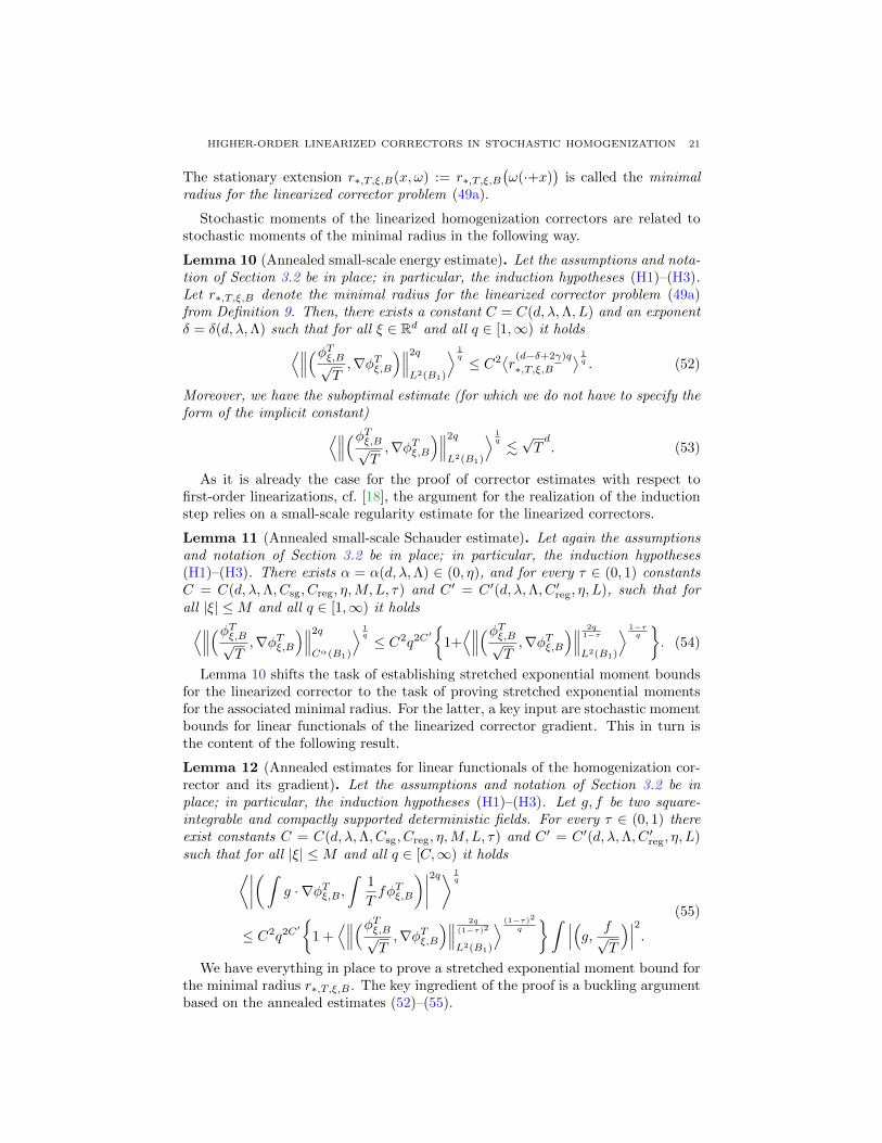
Lemma 10 shifts the task of establishing stretched exponential moment boundsfor the linearized corrector to the task of proving stretched exponential momentsfor the associated minimal radius. For the latter, a key input are stochastic momentbounds for linear functionals of the linearized corrector gradient. This in turn isthe content of the following result.

Lemma 12 (Annealed estimates for linear functionals of the homogenization cor-rector and its gradient). Let the assumptions and notation of Section 3.2 be inplace; in particular, the induction hypotheses (H1)–(H3). Let g, f be two square-integrable and compactly supported deterministic fields. For every τ ∈ (0, 1) thereexist constants C = C(d, λ,Λ, Csg, Creg, η,M,L, τ) and C ′ = C ′(d, λ,Λ, C ′reg, η, L)such that for all |ξ| ≤M and all q ∈ [C,∞) it holds⟨∣∣∣∣(ˆ g · ∇φTξ,B ,

ˆ1

TfφTξ,B

)∣∣∣∣2q⟩ 1q

≤ C2q2C′

1 +⟨∥∥∥(φTξ,B√

T,∇φTξ,B

)∥∥∥ 2q

(1−τ)2

L2(B1)

⟩ (1−τ)2

q

ˆ ∣∣∣(g, f√T

)∣∣∣2. (55)

We have everything in place to prove a stretched exponential moment bound forthe minimal radius r∗,T,ξ,B . The key ingredient of the proof is a buckling argumentbased on the annealed estimates (52)–(55).

22 SEBASTIAN HENSEL

Lemma 13 (Stretched exponential moment bound for minimal radius). Let theassumptions and notation of Section 3.2 be in place; in particular, the inductionhypotheses (H1)–(H3). Let r∗,T,ξ,B denote the minimal radius for the linearizedcorrector problem (49a) from Definition (9). Then, there exists γ = γ(d, λ,Λ), aswell as constants C = C(d, λ,Λ, Csg, Creg, η,M,L) and C ′ = C ′(d, λ,Λ, C ′reg, η, L)such that for all |ξ| ≤M and all q ≥ 1 it holds⟨

r2q∗,T,ξ,B

⟩ 1q ≤ C2q2C′ . (56)

A rather straightforward post-processing of Lemma 10, Lemma 11 and Lemma 12based on the stretched exponential moment bounds for the minimal radius fromLemma 13 now allows to conclude the induction step.

Lemma 14. Let the assumptions and notation of Section 3.2 be in place; in par-ticular, the induction hypotheses (H1)–(H3). Then the Lth-order linearized homog-enization corrector φTξ,B also satisfies (H1)–(H3).

3.5. Estimates for higher-order linearized flux correctors. In view of thedefining equations (49b) and (49c) for the linearized flux correctors, it is natural toestablish first the analogues of the estimates (39)–(43) for the linearized flux qTξ,B .

Actually, it suffices to establish the pendant of induction hypothesis (H2b). Thisis captured in the following result.

Lemma 15 (Sensitivity estimate for the linearized flux). Let the assumptions andnotation of Section 3.2 be in place. In particular, let qTξ,B be the linearized flux

as defined by (49d). Fix p ∈ (2,∞), and let g ∈⋂q≥1 L

2(Rd;L2q〈·〉) be a com-

pactly supported and Lp(Rd)-valued random field. Then there exists a random field

QTξ,B satisfying[QTξ,B

]1∈⋂q≥1 L

2q〈·〉L

2(Rd;Rn), and which is related to g via qTξ,Bin the sense that, P-almost surely, for all perturbations δω ∈ Cηuloc(Rd;Rn) with‖[δω]∞‖L2(Rd) <∞ it holds ˆ

g · δqTξ,B =

ˆQTξ,B · δω. (57)

In addition, there exist c0 = c0(d, λ,Λ) ∈ (1,∞), C ′ = C ′(d, λ,Λ, C ′reg, η, L)and C = C(d, λ,Λ, Csg, Creg, η,M,L) such that for all |ξ| ≤ M , all q ∈ [1,∞) andall q0 ∈ [ c0

c0−1 ,∞) the random field QTξ,B gives rise to a sensitivity estimate⟨∣∣∣∣ ˆ (−ˆB1(x)

|QTξ,B |)2∣∣∣∣q⟩ 1

q

≤ C2(q ∨ q0)2C′ sup〈F 2q∗ 〉=1

ˆ ⟨|Fg|2(q∨q0)∗

⟩ 1(q∨q0)∗ .

(58)

If (gr)r≥1 represents a sequence in⋂q≥1 L

2(Rd;L2q〈·〉) of compactly supported and

Lp(Rd)-valued random fields, denote by QT,rξ,B, r ≥ 1, the random field associated to

gr, r ≥ 1, in the sense of (57). Let g be an Lploc(Rd)-valued random field such that

gr → g as r →∞ in⋂q≥1 L

2(Rd;L2q〈·〉). Then there exists a random field QTξ,B with[

QT,rξ,B −QTξ,B

]1→ 0 as r →∞ in

⋂q≥1

L2q〈·〉L

2(Rd;Rn), (59)

and the sensitivity estimate (58) holds true in terms of (QTξ,B , g).

HIGHER-ORDER LINEARIZED CORRECTORS IN STOCHASTIC HOMOGENIZATION 23

Once this result is established, the asserted estimates in Theorem 5 for themassive linearized flux correctors (σTξ,B , ψ

Tξ,B) follow readily.

3.6. Differentiability of the massive correctors and the massive approx-imation of the homogenized operator. As a preparation for the proof of theestimates (23)–(25), which in particular contain estimates for differences of lin-earized correctors, and the higher-order differentiability of the homogenized opera-tor in form of Theorem 2, we establish the desired differentiability properties on thelevel of the massive approximation. A first step in this direction are the followingestimates for differences of linearized correctors.

Lemma 16 (Estimates for differences of linearized correctors). Let L ∈ N, M > 0as well as T ∈ [1,∞) be fixed. Let the requirements and notation of (A1), (A2)L,(A3)L and (A4)L of Assumption 1, (P1) and (P2) of Assumption 2, and (R) ofAssumption 3 be in place. We also fix a set of unit vectors v1, . . . , vL ∈ Rd anddefine B := v1 · · · vL.

For every β ∈ (0, 1), there exist constants C = C(d, λ,Λ, Csg, Creg, η,M,L, β)and C ′ = C ′(d, λ,Λ, C ′reg, η, L, β) such that for all |ξ| ≤ M , all q ∈ [1,∞), all unit

vectors e ∈ Rd and all |h| ≤ 1 it holds⟨∥∥(∇φTξ+he,B−∇φTξ,B ,∇σTξ+he,B−∇σTξ,B)∥∥2q

L2(B1)

⟩ 1q ≤ C2q2C′ |h|2(1−β), (60)⟨∥∥(∇φTξ+he,B−∇φTξ,B ,∇σTξ+he,B−∇σTξ,B)∥∥2q

Cα(B1)

⟩ 1q ≤ C2q2C′ |h|2(1−β), (61)

as well as for all compactly supported and square-integrable gφ, gσ⟨∣∣∣∣(ˆ gφ · (∇φTξ+he,B−∇φTξ,B),

ˆgklσ · (∇σTξ+he,B,kl−∇σTξ,B,kl)

)∣∣∣∣2q⟩ 1q

≤ C2q2C′ |h|2(1−β)

ˆ ∣∣(gφ, gσ)∣∣2. (62)

The already mentioned differentiability result for the massive linearized correc-tors and the massive approximation of the homogenized operator now reads asfollows.

Lemma 17 (Differentiability of massive correctors and the massive version of thehomogenized operator). Let L ∈ N, M > 0 and T ∈ [1,∞) be fixed. Let therequirements and notation of (A1), (A2)L, (A3)L and (A4)L of Assumption 1,(P1) and (P2) of Assumption 2, and (R) of Assumption 3 be in place. We also fixa set of unit vectors v1, . . . , vL ∈ Rd and define B := v1 · · · vL. Then, boththe maps ξ 7→ ∇φTξ,B and ξ 7→ ∇σTξ,B are Frechet differentiable with values in the

Frechet space L2〈·〉L

2loc(Rd).

Given a vector ξ ∈ Rd, a unit vector e ∈ Rd and some |h| ≤ 1 we define

ATB,e,h(ξ) :=⟨qTξ+he,B

⟩−⟨qTξ,B

⟩−⟨qTξ,Be

⟩h.

For every β ∈ (0, 1), there then exists C = C(d, λ,Λ, Csg, Creg, C′reg, η,M,L, β) such

that for all |ξ| ≤M , all unit vectors e ∈ Rd, and all |h| ≤ 1 it holds∣∣ATB,e,h(ξ)∣∣2 ≤ C2h4(1−β). (63)

Assume in addition to the above conditions that the stronger forms of (A2)L+1,(A3)L+1 and (A4)L+1 from Assumption 1 hold true. We then have the following

24 SEBASTIAN HENSEL

quantitative estimates on first-order Taylor expansions of the linearized correctorsφTξ,B and σTξ,B. Given a vector ξ ∈ Rd, a unit vector e ∈ Rd and some |h| ≤ 1, let

φTξ,B,e,h := φTξ+he,B − φTξ,B − φTξ,Beh,σTξ,B,e,h := σTξ+he,B − σTξ,B − σTξ,Beh.

For every β ∈ (0, 1), there then exist constants C = C(d, λ,Λ, Csg, Creg, η,M,L, β)and C ′ = C ′(d, λ,Λ, C ′reg, η, L, β) such that for all |ξ| ≤M , all unit vectors e ∈ Rd,all q ∈ [1,∞), all |h| ≤ 1 and all compactly supported and square-integrable gφ, gσit holds ⟨∥∥(∇φTξ,B,e,h,∇σTξ,B,e,h)∥∥2q

L2(B1)

⟩ 1q ≤ C2q2C′h4(1−β), (64)⟨∣∣∣∣(ˆ gφ · ∇φTξ,B,e,h,

ˆgklσ · ∇σTξ,B,e,h

)∣∣∣∣2q⟩ 1q

≤ C2q2C′ |h|4(1−β)

ˆ ∣∣(gφ, gσ)∣∣2.(65)

Remark 18. In case of q = 1, the estimates (64) and (65) actually hold truerequiring only (A2)L, (A3)L and (A4)L from Assumption 1. This in turn repre-sents exactly the form of Assumption 1 for which qualitative differentiability of thelinearized corrector gradients is established in Lemma 17. A proof of this claim iscontained in the proof of Lemma 17.

3.7. The limit passage in the massive approximation. The last main ingredi-ent in the proof of Theorem 1 and Theorem 2 consists of studying the limit T →∞in the massive approximation. More precisely, we establish the following result.

Lemma 19 (Limit passage in the massive approximation). Let L ∈ N and M > 0be fixed. Let the requirements and notation of (A1), (A2)L and (A3)L of Assump-tion 1, (P1) and (P2) of Assumption 2, and (R) of Assumption 3 be in place. Wealso fix a set of unit vectors v1, . . . , vL ∈ Rd and define B := v1 · · · vL.

Then the sequence (∇φTξ,B , ∇σTξ,B

)T∈[1,∞)

is Cauchy in L2〈·〉L

2loc(Rd) (with respect to the strong topology). Moreover, there

exists C = C(d, λ,Λ, Csg, Creg, C′reg, η,M,L) such that for all |ξ| ≤ M and all

T ∈ [1,∞) we have the estimates

⟨∥∥(∇φ2Tξ,B −∇φTξ,B ,∇σ2T

ξ,B −∇σTξ,B)∥∥2

L2(B1)

⟩≤ C2

(µ2∗(√T )

T

) 1

2L

, (66)∣∣⟨q2Tξ,B

⟩−⟨qTξ,B

⟩∣∣2 ≤ C2(µ2∗(√T )

T

) 1

2L

. (67)

The corresponding limits give rise to higher-order linearized homogenization correc-tors and flux correctors in the sense of Definition 4. Moreover,⟨∣∣qTξ,B − qξ,B∣∣2⟩→ 0, (68)

with the limiting linearized flux qξ,B defined in (30b).

HIGHER-ORDER LINEARIZED CORRECTORS IN STOCHASTIC HOMOGENIZATION 25

4. Proofs

4.1. Proof of Lemma 10 (Annealed small-scale energy estimate). Applying thehole filling estimate (T2) to equation (49a) for the linearized homogenization correc-tor (putting the term −∇ · aTξ 1L=1B on the right hand side) yields in combination

with (A2)L from Assumption 1∥∥∥(φTξ,B√T,∇φTξ,B

)∥∥∥2

L2(B1)

.d,λ,Λ,L rd−δ∗,T,ξ,B1L=1 + rd−δ∗,T,ξ,B −

ˆBr∗,T,ξ,B

∣∣∣(φTξ,B√T,∇φTξ,B

)∣∣∣2+ rd∗,T,ξ,B

∑Π∈Par1,...,LΠ6=1,...,L

−ˆBr∗,T,ξ,B

1

|x|δ∏π∈Π

∣∣1|π|=1B′π +∇φTξ,B′π

∣∣2.For the second right hand side term, we proceed by making use of Caccioppoli’sinequality (T1) with respect to equation (49a); and in the course of this we againrely on (A2)L from Assumption 1 in order to bound the right hand side termappearing in equation (49a). For the third right hand side term, we simply argueby Holder’s inequality. In total, we obtain the estimate∥∥∥(φTξ,B√

T,∇φTξ,B

)∥∥∥2

L2(B1)

.d,λ,Λ,L rd−δ∗,T,ξ,B1L=1

+ rd−δ∗,T,ξ,B infb∈R

1

(2r∗,T,ξ,B)2−ˆB2r∗,T,ξ,B

∣∣φTξ,B−b∣∣2 +1

T|b|2

+ rd−δ∗,T,ξ,B

∑Π∈Par1,...,LΠ6=1,...,L

−ˆB2r∗,T,ξ,B

∏π∈Π

∣∣1|π|=1B′π +∇φTξ,B′π

∣∣2

+ rd−δ∗,T,ξ,B

∑Π∈Par1,...,LΠ6=1,...,L

∏π∈Π

(−ˆBr∗,T,ξ,B

∣∣1|π|=1B′π +∇φTξ,B′π

∣∣4|Π|) 12|Π|

.

Taking into account Definition 9 of the minimal radius, the fact that r∗,T,ξ,B ≥ 1,as well as Holder’s and Jensen’s inequality (to deal with the second right hand sideterm in the previous display) we deduce from this∥∥∥(φTξ,B√

T,∇φTξ,B

)∥∥∥2

L2(B1).d,λ,Λ,L r

d−δ+2γ∗,T,ξ,B .

Taking stochastic moments thus entails the asserted estimate (52).For a proof of (53), we rely on the weighted energy estimate (T3). In order to

apply it, we first have to check the polynomial growth at infinity (in the precisesense of the statement of Lemma 21) of the constituents in the linearized correctorproblem (49a). For the solution (φTξ,B ,∇φTξ,B) itself, this is a consequence of the

fact that φTξ,B ∈ H1uloc(Rd). For the right hand side term in equation (49a) we

argue as follows. First, thanks to the ergodic theorem we may choose almost surely

26 SEBASTIAN HENSEL

a radius R0 > 0 such that

−ˆBR

∏π∈Π

∣∣1|π|=1B′π +∇φTξ,B′π

∣∣2≤ 1 +

⟨ ∏π∈Π

∣∣1|π|=1B′π +∇φTξ,B′π

∣∣2⟩ for all R ≥ R0,(69)

uniformly over all partitions Π ∈ Par1, . . . , L with Π 6= 1, . . . , L. Thanks tothe induction hypothesis (H1) and (H3), we may then smuggle in spatial averagesover the unit ball B1 followed by an application of Holder’s inequality to deducethat⟨ ∏

π∈Π

∣∣1|π|=1B′π +∇φTξ,B′π

∣∣2⟩.⟨ ∏π∈Π

∥∥1|π|=1B′π +∇φTξ,B′π

∥∥2

Cα(B1)

⟩+⟨ ∏π∈Π

ˆB1

∣∣1|π|=1B′π +∇φTξ,B′π

∣∣2⟩.∏π∈Π

⟨∥∥1|π|=1B′π +∇φTξ,B′π

∥∥2|Π|Cα(B1)

⟩ 1|Π|

+∏π∈Π

⟨∥∥1|π|=1B′π +∇φTξ,B′π

∥∥2|Π|L2(B1)

⟩ 1|Π|

. 1,

uniformly over all partitions Π ∈ Par1, . . . , L with Π 6= 1, . . . , L. Insertingthis back into (69) shows that also the right hand side terms of equation (49a)feature at most polynomial growth at infinity.

Hence, we may apply the weighted energy estimate (T3) to equation (49a) whichentails in combination with Jensen’s and Holder’s inequality⟨∥∥∥(φTξ,B√

T,∇φTξ,B

)∥∥∥2q

L2(B1)

⟩ 1q

.√Td1L=1 +

√Td ∑

Π∈Par1,...,LΠ6=1,...,L

ˆ`γ,√T

⟨ ∏π∈Π

∣∣1|π|=1B′π +∇φTξ,B′π

∣∣2q⟩ 1q

.√Td1L=1 +

√Td ∑

Π∈Par1,...,LΠ6=1,...,L

ˆ`γ,√T

∏π∈Π

⟨∣∣1|π|=1B′π +∇φTξ,B′π

∣∣2q|Π|⟩ 1q|Π|

.

Taking into account the induction hypothesis (H1) and (H3)—the latter in particu-lar allowing us to smuggle in a spatial average over unit balls B1(x)— and makinguse of stationarity of the linearized homogenization correctors, we thus infer fromthe previous display the asserted estimate (53).

4.2. Proof of Lemma 11 (Annealed small-scale Schauder estimate). We aim toapply the local Schauder estimate (T5) to equation (49a) for the linearized homog-enization corrector (putting to this end the term −∇ · aTξ 1L=1B on the right hand

side). This is facilitated by the annealed Holder regularity of the linearized coeffi-cient field aTξ = (∂ξA)(ω, ξ +∇φTξ ), cf. Lemma 24 in Appendix A. Hence, in view

of the local Schauder estimate (T5) we may estimate by an application of Holder’s

HIGHER-ORDER LINEARIZED CORRECTORS IN STOCHASTIC HOMOGENIZATION 27

inequality with respect to the exponents ( 1τ ,

11−τ ), τ ∈ (0, 1),

⟨∥∥∥(φTξ,B√T,∇φTξ,B

)∥∥∥2q

Cα(B1)

⟩ 1q

≤ C2⟨∥∥aTξ ∥∥ 2q

τdα ( 1

2 + 1d )

Cα(B2)

⟩ τq

⟨∥∥∥(φTξ,B√T,∇φTξ,B

)∥∥∥ 2q1−τ

L2(B2)

⟩ 1−τq

+ C2⟨∥∥aTξ ∥∥4q( 1

α−1)

Cα(B2)

⟩ 12q

∑Π∈Par1,...,LΠ6=1,...,L

⟨∥∥∥ ∏π∈Π

∣∣1|π|=1B′π +∇φTξ,B′π

∣∣∥∥∥4q

Cα(B2)

⟩ 12q

+ C2⟨∥∥aTξ ∥∥ 2q

α

Cα(B2)

⟩ 1q 1L=1.

A combination of the annealed estimate (T7) for the Holder norm of the linearizedcoefficient, the small-scale annealed Schauder estimate from induction hypothe-sis (H3), the stationarity of the linearized coefficient field and of the linearizedhomogenization correctors, and Holder’s inequality updates the previous display to⟨∥∥∥(φTξ,B√

T,∇φTξ,B

)∥∥∥2q

Cα(B1)

⟩ 1q

≤ C2q2C′

1 +⟨∥∥∥(φTξ,B√

T,∇φTξ,B

)∥∥∥ 2q1−τ

L2(B1)

⟩ 1−τq

+ C2q2C′

∑Π∈Par1,...,LΠ6=1,...,L

∏π∈Π

⟨∥∥∥∣∣1|π|=1B′π +∇φTξ,B′π

∣∣∥∥∥4q|Π|

Cα(B1)

⟩ 12q|Π|

≤ C2q2C′

1 +⟨∥∥∥(φTξ,B√

T,∇φTξ,B

)∥∥∥ 2q1−τ

L2(B1)

⟩ 1−τq

.

This concludes the proof of Lemma 11.

4.3. Proof of Lemma 12 (Annealed estimates for linear functionals of the ho-mogenization corrector and its gradient). The proof proceeds in three steps. In thecourse of it, we will make use of the abbreviation

∑Π :=

∑Π∈Par1,...,L,Π6=1,...,L.

Since (φTξ,B√T,∇φTξ,B) ∈ L2

uloc(Rd;R×Rd), we may assume for the proof of (55) with-

out loss of generality through an approximation argument that P-almost surely

(g, f) ∈ C∞cpt(Rd;Rd×R). (70)

Step 1 (Computation of functional derivative): We start by computing the func-tional derivative of

Fφ :=

ˆg · ∇φTξ,B −

ˆ1

TfφTξ,B . (71)

To this end, consider a perturbation δω ∈ Cηuloc(Rd;Rn) with ‖[δω]∞‖L2(Rd) < ∞.Based on Lemma 26, we may P-almost surely differentiate the defining equa-tion (49a) for the linearized homogenization corrector with respect to the parameterfield in the direction of δω. This yields P-almost surely the following PDE for the

28 SEBASTIAN HENSEL

variation (δφTξ,B√T,∇δφTξ,B) ∈ L2

uloc(Rd;R×Rd) ∩ Lperg(Rd;R×Rd), p ≥ 2, of the lin-

earized corrector φTξ,B with massive term:

1

TδφTξ,B −∇ · aTξ ∇δφTξ,B

= ∇ · (∂ω∂ξA)(ω, ξ +∇φTξ )[δω ∇φTξ,B

]+∇ · (∂2

ξA)(ω, ξ +∇φTξ )[∇δφTξ ∇φTξ,B

]+∇ ·

∑Π

(∂ω∂|Π|ξ A)(ω, ξ+∇φTξ )

[δω

⊙π∈Π

(1|π|=1B′π+∇φTξ,B′π )

]+∇ ·

∑Π

(∂1+|Π|ξ A)(ω, ξ+∇φTξ )

[∇δφTξ

⊙π∈Π

(1|π|=1B′π+∇φTξ,B′π )

]+∇ ·

∑Π

(∂|Π|ξ A)(ω, ξ+∇φTξ )

[∑π∈Π

∇δφTξ,B′π ⊙π′∈Ππ′ 6=π

(1|π′|=1B′π′+∇φTξ,B′

π′)]

=: ∇ ·RT,(1)ξ,B δω +∇ ·RT,(2)

ξ,B ∇δφTξ +∇ ·RT,(3)

ξ,B δω +∇ ·RT,(4)ξ,B ∇δφ

Tξ (72)

+∑Π

∑π∈Π

∇ ·RT,(5),πξ,B ∇δφTξ,B′π .

Observe that as a consequence of (51) and (A2)L resp. (A3)L of Assumption 1 wehave P-almost surely

RT,(1)ξ,B , R

T,(3)ξ,B ∈ Lperg(Rd;Rd×n), R

T,(2)ξ,B , R

T,(4)ξ,B , R

T,(5),πξ,B ∈ Lperg(Rd;Rd×d) (73)

for all p ≥ 2. For r ≥ 1, let (δφT,rξ,B√T,∇δφT,rξ,B) ∈ L2(Rd;R×Rd) be the unique Lax–

Milgram solution of

1

TδφT,rξ,B −∇ · a

Tξ ∇δφ

T,rξ,B

=: ∇ · 1BrRT,(1)ξ,B δω +∇ · 1BrR

T,(2)ξ,B ∇δφ

Tξ +∇ · 1BrR

T,(3)ξ,B δω (74)

+∇ · 1BrRT,(4)ξ,B ∇δφ

Tξ +

∑Π

∑π∈Π

∇ · 1BrRT,(5),πξ,B ∇δφTξ,B′π .

Note that P-almost surely

(δφT,rξ,B√T,∇δφT,rξ,B

)→(δφTξ,B√

T,∇δφTξ,B

)as r →∞ in L2

uloc(Rd;Rd×d) (75)

by means of applying the weighted energy estimate (T3) to the difference of theequations (72) and (74).

HIGHER-ORDER LINEARIZED CORRECTORS IN STOCHASTIC HOMOGENIZATION 29

Denoting the transpose of aTξ by aT,∗ξ , we may now compute by means of Lemma 26,

(73), (74), (75) and (189)

δFφ =

ˆg · ∇δφTξ,B −

ˆ1

TfδφTξ,B

= limr→∞

ˆg · ∇δφT,rξ,B −

ˆ1

TfδφT,rξ,B

= − lim

r→∞

ˆ∇δφT,rξ,B · a

T,∗ξ ∇

( 1

T−∇ · aT,∗ξ ∇

)−1( 1

Tf+∇ · g

)+

ˆδφT,rξ,B

1

T

( 1

T−∇ · aT,∗ξ ∇

)−1( 1

Tf+∇ · g

)= limr→∞

ˆ1BrR

T,(1)ξ,B δω · ∇

( 1

T−∇ · aT,∗ξ ∇

)−1( 1

Tf+∇ · g

)(76)

+

ˆ1BrR

T,(2)ξ,B ∇δφ

Tξ · ∇

( 1

T−∇ · aT,∗ξ ∇

)−1( 1

Tf+∇ · g

)+

ˆ1BrR

T,(3)ξ,B δω · ∇

( 1

T−∇ · aT,∗ξ ∇

)−1( 1

Tf+∇ · g

)+

ˆ1BrR

T,(4)ξ,B ∇δφ

Tξ · ∇

( 1

T−∇ · aT,∗ξ ∇

)−1( 1

Tf+∇ · g

)+∑Π

∑π∈Π

ˆ1BrR

T,(5),πξ,B ∇δφTξ,B′π · ∇

( 1

T−∇ · aT,∗ξ ∇

)−1( 1

Tf+∇ · g

).

Note that thanks to the approximation argument, the regularity (73) as well as

the regularity (189), we may indeed use δφT,rξ,B as a test function in the equation of(1T−∇·a

T,∗ξ ∇

)−1( 1T f+∇·g

)and vice versa. Moreover, by (73), the assumption (70)

ensuring that (g, f) are Lp(Rd)-valued random fields for any p > 2, and the (local)

Meyers estimate for the operator ( 1T −∇ · a

T,∗ξ ∇), we obtain that P-almost surely

(RT,(i)ξ,B

)∗∇( 1

T−∇ · aT,∗ξ ∇

)−1( 1

Tf+∇ · g

)∈ Lp

′

loc(Rd;Rn), i ∈ 1, 3,(RT,(i)ξ,B

)∗∇( 1

T−∇ · aT,∗ξ ∇

)−1( 1

Tf+∇ · g

)∈ Lp

′

loc(Rd;Rd), i ∈ 2, 4,(RT,(5),πξ,B

)∗∇( 1

T−∇ · aT,∗ξ ∇

)−1( 1

Tf+∇ · g

)∈ Lp

′

loc(Rd;Rd)

(77)

for some suitable Meyers exponent p′ > 2. We have everything in place to proceedwith the next step of the proof.

Step 2 (Application of the spectral gap inequality): Note first that 〈Fφ〉 = 0 forthe functional Fφ from (71). Indeed, 〈(φTξ,B ,∇φTξ,B)〉 = 0 is a direct consequence

of stationarity and testing the linearized corrector problem (49a). Hence, we mayapply the spectral gap inequality in form of (48) and thus obtain in view of (A2)Land (A3)L of Assumption 1, (76), (77), induction hypotheses (H2a) and (H2c),and the sensitivity estimates from induction hypothesis (H2b) the estimate (with

30 SEBASTIAN HENSEL

κ1, κ2 ∈ (0, 1] yet to be determined)⟨∣∣Fφ∣∣2q⟩ 1q

≤ C2q2

⟨∣∣∣∣ˆ (−ˆB1(x)

∣∣∇φTξ,B∣∣2)(−ˆB1(x)

∣∣∣( 1

T−∇ · aT,∗ξ ∇

)−1( 1

Tf+∇ · g

)∣∣∣2)∣∣∣∣q⟩ 1q

+ C2q2∑Π

⟨∣∣∣∣ˆ (−ˆB1(x)

∏π∈Π

∣∣1|π|=1B′π+∇φTξ,B′π

∣∣2)

×(−ˆB1(x)

∣∣∣∇( 1

T−∇ · aT,∗ξ ∇

)−1( 1

Tf+∇ · g

)∣∣∣2)∣∣∣∣q⟩ 1q

+ C2(q ∨ q0)2C′ sup〈F 2q∗ 〉=1

ˆ ⟨∣∣∣∇φTξ,B∣∣∣2(q∨q0κ1

)∗ ∣∣∣∇( 1

T−∇ · aT,∗ξ ∇

)−1( 1

TFf+∇ · Fg

)∣∣∣2(q∨q0κ1

)∗⟩ 1

(q∨q0κ1

)∗

+ C2(q ∨ q0)2C′∑Π

sup〈F 2q∗ 〉=1

ˆ ⟨∣∣∣∇( 1

T−∇ · aT,∗ξ ∇

)−1( 1

TFf+∇ · Fg

)∣∣∣2(q∨q0κ2

)∗

×∏π∈Π

∣∣1|π|=1B′π+∇φTξ,B′π

∣∣2(q∨q0κ2

)∗⟩ 1

(q∨q0κ2

)∗

+ C2(q ∨ q0)2C′∑Π

∑π∈Π

sup〈F 2q∗ 〉=1

ˆ ⟨∣∣∣∇( 1

T−∇ · aT,∗ξ ∇

)−1( 1

TFf+∇ · Fg

)∣∣∣2(q∨q0κ2

)∗

×∏π′∈Ππ′ 6=π

∣∣1|π′|=1B′π′+∇φTξ,B′

π′

∣∣2(q∨q0κ2

)∗⟩ 1

(q∨q0κ2

)∗

=: I1 + I2 + I3 + I4 + I5. (78)

For the last three right hand side terms in the previous display, we also exploited thefact that F is purely random so that one can simply multiply with F the equation

satisfied by ( 1T −∇ · a

T,∗ξ ∇)−1( 1

T f +∇ · g).

Step 3 (Post-processing the right hand side of (78)): We estimate each of theright hand side terms of (78) separately. By duality in Lq〈·〉, stationarity of the

linearized homogenization corrector φTξ,B , and Holder’s inequality with respect to

the exponents ( q∨q01−τ , (q∨q01−τ )∗), τ ∈ (0, 1), we estimate the contribution from I1 by

|I1| ≤ C2q2⟨∥∥∥(φTξ,B√

T,∇φTξ,B

)∥∥∥ 2(q∨q0)1−τ

L2(B1)

⟩ 1−τq∨q0

× sup〈F 2q∗ 〉=1

ˆ−ˆB1(x)

⟨∣∣∣∇( 1

T−∇ · aT,∗ξ ∇

)−1( 1

TFf+∇ · Fg

)∣∣∣2(q∨q01−τ )∗⟩ 1

(q∨q01−τ )∗ .

As ( q∨q01−τ )∗ = q∨q0(q∨q0)−(1−τ) ≤

q∨q0(q∨q0)−1 = (q ∨ q0)∗ ≤ q∗ ∧ (q0)∗, it follows from

Jensen’s inequality, the fact that´−B1(x)

h =´h for all non-negative h, and the

annealed Calderon–Zygmund estimate (T8) that

|I1| ≤ C2q2⟨∥∥∥(φTξ,B√

T,∇φTξ,B

)∥∥∥ 2(q∨q0)1−τ

L2(B1)

⟩ 1−τq∨q0

sup〈F 2q∗ 〉=1

ˆ ⟨∣∣∣( Ff√T, Fg

)∣∣∣2q∗⟩ 1q∗

≤ C2q2⟨∥∥∥(φTξ,B√

T,∇φTξ,B

)∥∥∥ 2(q∨q0)1−τ

L2(B1)

⟩ 1−τq∨q0ˆ ∣∣∣( f√

T, g)∣∣∣2 (79)

HIGHER-ORDER LINEARIZED CORRECTORS IN STOCHASTIC HOMOGENIZATION 31

provided |(q0)∗−1| is sufficiently small (depending only on d, λ,Λ). In other words,we obtain a bound of required type for all q ≥ q0 with q0 ∈ [1,∞) sufficiently large.

For the contribution from I2, we may estimate based on the same ingredients asin the estimate of I1 (we could actually take τ = 0 but prefer to keep the generalform for later reference) for all sufficiently large q0 ∈ [1,∞) and all q ∈ [1,∞)

|I2| ≤ C2q2∑Π

∏π∈Π

⟨−ˆB1

∣∣1|π|=1B′π+∇φTξ,B′π

∣∣ 2(q∨q0)|Π|1−τ

⟩ 1−τ(q∨q0)|Π|

× sup〈F 2q∗ 〉=1

ˆ−ˆB1(x)

⟨∣∣∣∇( 1

T−∇ · aT,∗ξ ∇

)−1( 1

TFf+∇ · Fg

)∣∣∣2(q∨q01−τ )∗⟩ 1

(q∨q01−τ )∗

≤ C2q2C

ˆ ∣∣∣( f√T, g)∣∣∣2, (80)

where in the second step we in addition made use of the small-scale annealedSchauder estimate from induction hypothesis (H3) (by smuggling in a spatial aver-age over the unit ball) and the corrector estimates from induction hypothesis (H1).

We next estimate the contribution from I3. To this end, we first choose κ1 = τ2

and then estimate via stationarity of the linearized homogenization corrector φTξ,B ,

the fact that ( q∨q0κ1)∗ = q∨q0

(q∨q0)−κ1, an application of Holder’s inequality with respect

to the exponents ( (q∨q0)−κ1

1−τ , ( (q∨q0)−κ1

1−τ )∗), and an application of Jensen’s inequality

based on ( q∨q0κ1)∗(

(q∨q0)−κ1

1−τ )∗ = q∨q0(q∨q0)−κ1−(1−τ) ≤

q∨q0(q∨q0)−1 = (q ∨ q0)∗ ≤ q∗ ∧ (q0)∗

|I3| ≤ C2(q ∨ q0)2C′⟨∥∥∇φTξ,B∥∥ 2(q∨q0)

1−τCα(B1)

⟩ q∨q01−τ

× sup〈F 2q∗ 〉=1

ˆ ⟨∣∣∣∇( 1

T−∇ · aT,∗ξ ∇

)−1( 1

TFf+∇ · Fg

)∣∣∣2q∗⟩ 1q∗.

Hence, by means of the annealed Calderon–Zygmund estimate (T8) and the an-nealed small-scale Schauder estimate (54) (with q replaced by q∨q0

1−τ ) we obtain

|I3| ≤ C2(q ∨ q0)2C′⟨∥∥∥(φTξ,B√

T,∇φTξ,B

)∥∥∥ 2(q∨q0)

(1−τ)2

L2(B1)

⟩ (1−τ)2

q∨q0ˆ ∣∣∣( f√

T, g)∣∣∣2, (81)

at least for sufficiently large q0 ∈ [1,∞). This in turn is again a bound of requiredtype for all q ≥ q0.

We next deal with the contribution from I4. To this end, we simply chooseκ2 = 1

2 and argue based on stationarity of the linearized homogenization correc-

tors, ( q∨q0κ2)∗ = q∨q0

(q∨q0)−κ2, an application of Holder’s inequality with respect to

the exponents ( (q∨q0)−κ2

(q∨q0)−1 , ((q∨q0)−κ2

(q∨q0)−1 )∗), and the fact that ( q∨q0κ2)∗(

(q∨q0)−κ2

(q∨q0)−1 )∗ =q∨q01−κ2

= 2(q ∨ q0)

|I4| ≤ C2(q ∨ q0)2C′∑Π

∏π∈Π

⟨∣∣1|π|=1B′π+∇φTξ,B′π

∣∣4(q∨q0)|Π|⟩ 1

2(q∨q0)|Π|

× sup〈F 2q∗ 〉=1

ˆ ⟨∣∣∣∇( 1

T−∇ · aT,∗ξ ∇

)−1( 1

TFf+∇ · Fg

)∣∣∣2(q∨q0)∗⟩ 1(q∨q0)∗

.

As it is by now routine, the second factor of the right hand side term of the previousdisplay is dealt with by appealing to the annealed Calderon–Zygmund estimate (T8)for which we only have to choose q0 ∈ [1,∞) sufficiently large. For the first factor,

32 SEBASTIAN HENSEL

we may smuggle in a spatial average over the ball B1 and then estimate by meansof the induction hypotheses (H1) and (H3). In total, we obtain for all q ∈ [1,∞)

|I4| ≤ C2(q ∨ q0)2C′ˆ ∣∣∣( f√

T, g)∣∣∣2 (82)

provided q0 ∈ [1,∞) is sufficiently large. As the contribution from I5 can be treatedanalogously, the combination of the estimates (79)–(82) establishes the assertedbound (55). This concludes the proof of Lemma 12.

4.4. Proof of Lemma 13 (Stretched exponential moment bound for minimalradius of the linearized corrector problem). We start with the estimate

⟨r

(d− δ2 )2q

∗,T,ξ,B⟩≤ 1 +

∞∑k=1

2k(d− δ2 )2qP[r∗,T,ξ,B = 2k

]. (83)

Fix an integer k ≥ 1, and let R := 2k. By Definition 9 of the minimal radiusr∗,T,ξ,B , in the event of r∗,T,ξ,B = R we either have

∃Π ∈ Par1, . . . , L, Π 6= 1, . . . , L : ∃π ∈ Π such that

−ˆBR

2

∣∣1|π|=1B′π +∇φTξ,B′π

∣∣4|Π| > (R2

)4γ

, (84)

or that

infb∈R

1

(R/2)2−ˆBR

2

∣∣φTξ,B−b∣∣2+1

T|b|2> 1. (85)

We distinguish in the following between these two events, and provide separatelyan estimate on their probability.

Case 1: (Estimate in the event of (84)) Fix a partition Π ∈ Par1, . . . , L,Π 6= 1, . . . , L, and some π ∈ Π such that the conclusion of (84) holds true.Covering BR

2by a family of ∼ Rd many open unit balls, using stationarity of the

linearized homogenization correctors, Jensen’s inequality, the small-scale annealedSchauder estimate from induction hypothesis (H3) which in particular allows tosmuggle in a spatial average over the unit ball, and finally the corrector boundsfrom induction hypotheses (H1), we infer that⟨∣∣∣∣−ˆ

BR2

∣∣1|π|=1B′π +∇φTξ,B′π

∣∣4|Π|∣∣∣∣2q⟩ 1q

≤ C2q2C′

for all q ∈ [1,∞). It thus follows from Markov’s inequality and the previous display(with q replaced by γ−1dq) that

P[r∗,T,ξ,B = 2k

∩ (84) holds true

]≤ C2qq2C′q2−k8dq (86)

with constants C = C(d, λ,Λ, Csg, Creg, η,M,L) and C ′ = C ′(d, λ,Λ, C ′reg, η, L).Case 2: (Suboptimal estimate in the event of (85) but not (84)) Let 0 < R′ ≤ R,

and abbreviate by (h)R′(x) := −BR′ (x)

h the mollification on scale R′ for any locally

integrable h. In the event of (85) holds true ∩ (84) holds not true we deduce

HIGHER-ORDER LINEARIZED CORRECTORS IN STOCHASTIC HOMOGENIZATION 33

from the triangle inequality that

1 .1

R2−ˆBR

∣∣φTξ,B−(φTξ,B)R′∣∣2

+1

R2−ˆBR

∣∣∣∣(φTξ,B)R′−−ˆBR

(φTξ,B)R′

∣∣∣∣2 +1

T

∣∣∣∣−ˆBR

(φTξ,B)R′

∣∣∣∣2. (87)

The first term on the right hand side of the previous display is estimated by

1

R2−ˆBR

∣∣φTξ,B−(φTξ,B)R′∣∣2 . (R′

R

)2

−ˆB2R

∣∣∇φTξ,B∣∣2,the second right hand side term based on Poincare’s inequality and the definitionof (·)R′ by

1

R2−ˆBR

∣∣∣∣(φTξ,B)R′−−ˆBR

(φTξ,B)R′

∣∣∣∣2 . −ˆB2R

∣∣∣∣−ˆBR′ (x)

∇φTξ,B∣∣∣∣2,

and the third right hand side term simply by plugging in the definition of (·)R′ andJensen’s inequality

1

T

∣∣∣∣−ˆBR

(φTξ,B)R′

∣∣∣∣2 . −ˆB2R

∣∣∣∣−ˆBR′ (x)

1√TφTξ,B

∣∣∣∣2.In the event of (85) holds true ∩ (84) holds not true, the combination of thelast four displays therefore entails

1 .(R′R

)2

−ˆB2R

∣∣∇φTξ,B∣∣2 +−ˆB2R

∣∣∣∣−ˆBR′ (x)

∇φTξ,B∣∣∣∣2 +−ˆB2R

∣∣∣∣−ˆBR′ (x)

1√TφTξ,B

∣∣∣∣2. (88)

Applying next the Caccioppoli inequality (T1) to equation (49a) for the linearizedhomogenization corrector (putting the term −∇·aTξ 1L=1B on the right hand side),and making use of Definition 9 of the minimal radius r∗,T,ξ,B we obtain in the eventof (85) holds true ∩ (84) holds not true(R′

R

)2

−ˆB2R

∣∣∇φTξ,B∣∣2 ≤ C(d, λ,Λ)(R′R

)2(1 +R2γ

). (89)

Hence, restricting γ = γ(d, λ,Λ) ∈ (0, 12 ) (but otherwise yet to be determined),

choosing R′ = θR1−γ with θ = θ(d, λ,Λ) such that 2θ2C(d, λ,Λ) = 12 , we infer

from (88) and (89) in the event of (85) holds true ∩ (84) holds not true

1 .d,λ,Λ −ˆB2R

∣∣∣∣−ˆBθR

1−γ (x)

∇φTξ,B∣∣∣∣2 +−ˆB2R

∣∣∣∣−ˆBθR

1−γ (x)

1√TφTξ,B

∣∣∣∣2. (90)

It thus follows from an application of Markov’s inequality in combination withstationarity of the linearized homogenization correctors and Jensen’s inequalitythat

P[r∗,T,ξ,B = 2k

∩ (85) holds true ∩ (84) holds not true

]≤ C(d, λ,Λ)2q

⟨∣∣∣∣−ˆBθ2k(1−γ)

∇φTξ,B , −ˆBθ2k(1−γ)

1√TφTξ,B

∣∣∣∣4q⟩. (91)

Thanks to the moment bounds (55) for linear functionals of the linearized homog-enization corrector and its gradient (applied with, say, τ = 1

2 ) in combination with

34 SEBASTIAN HENSEL

the suboptimal small-scale energy estimate (53), we get the following update of theprevious display

P[r∗,T,ξ,B = 2k

∩ (85) holds true ∩ (84) holds not true

].d,λ,Λ,q

√T

2dq2−k(1−γ)2dq,

(92)

which is—with respect to the scaling in the stochastic integrability q and the massiveapproximation T—a highly supobtimal estimate for this probability.

Intermediate summary: (Suboptimal estimate on stochastic moments of the min-imal radius) We collect the information provided by the estimates (86) and (92),and combine it with (83) resulting in

⟨r

(d− δ2 )2q

∗,T,ξ,B⟩≤ 1 + C2qq2C′q

∞∑k=1

2k(d− δ2 )2q2−k8dq

+ Cq√T

2dq∞∑k=1

2k(d− δ2 )2q2−k(1−γ)2dq

(93)

with constants C = C(d, λ,Λ, Csg, Creg, η,M,L) and C ′ = C ′(d, λ,Λ, C ′reg, η, L),

and a constant Cq which in addition depends in a possibly highly suboptimal way

on q ∈ [1,∞). Choosing γ := 12 ∧

δ4d thus entails the suboptimal estimate⟨

r(d− δ2 )2q

∗,T,ξ,B⟩≤ Cq

√T

2dq. (94)

Conclusion: (From suboptimal moment bounds to stretched exponential moments)The merit of (94) is that it at least provides finiteness of arbitrarily high stochasticmoments of the minimal radius r∗,T,ξ,B . We now leverage on that information in abuckling argument. We observe from the previous argument that suboptimality wasonly a result of using (55) with a non-optimized τ ∈ (0, 1) and using the suboptimalsmall-scale energy estimate (53) in order to transition from (91) to (92).

If we instead apply (55) with τ ∈ (0, 1) yet to be optimized, and then feed inthe annealed small-scale energy estimate from Lemma 10 in form of (52) (with qreplaced by 2q

(1−τ)2 ), we may update (92) to

P[r∗,T,ξ,B = 2k

∩ (85) holds true ∩ (84) holds not true

]≤ C2qq2C′q2−k(1−γ)2dq

⟨r

d−δ+2γ

(1−τ)22q

∗,T,ξ,B

⟩(1−τ)2

,(95)

with constants C = C(d, λ,Λ, Csg, Creg, η,M,L, τ) and C ′ = C ′(d, λ,Λ, C ′reg, η, L).This in turn provides the following improvement of (93)

⟨r

(d− δ2 )2q

∗,T,ξ,B⟩≤ C2qq2C′q + C2qq2C′q

∞∑k=1

2k(d− δ2 )2q2−k(1−γ)2dq⟨r

d−δ+2γ

(1−τ)22q

∗,T,ξ,B

⟩(1−τ)2

.

Choosing γ := 12 ∧

δ8d and then τ ∈ (0, 1) such that

d−δ+2γ

(1−τ)2 = d− δ2 we obtain⟨

r(d− δ2 )2q

∗,T,ξ,B⟩≤ C2qq2C′q

(1 +

⟨r

(d− δ2 )2q

∗,T,ξ,B⟩(1−τ)2)

.

Because of (94) and r∗,T,ξ,B ≥ 1, this concludes the proof of Lemma 13.

HIGHER-ORDER LINEARIZED CORRECTORS IN STOCHASTIC HOMOGENIZATION 35

4.5. Proof of Lemma 14 (Conclusion of the induction step). The validity of thecorrector bounds from (H1) with φTξ,B′ replaced by φTξ,B is an immediate conse-

quence of (52), (55), and (56). The small-scale annealed Schauder estimate frominduction hypothesis (H3) with φTξ,B′ replaced by φTξ,B follows from combining (52),

(54), and (56).It remains to establish induction hypotheses (H2a)–(H2c) with φTξ,B′ replaced

by φTξ,B . Starting point is the following reminder of (76)

ˆg · ∇δφTξ,B −

ˆ1

TfδφTξ,B

= − limr→∞

ˆ∇δφT,rξ,B · a

T,∗ξ ∇

( 1

T−∇ · aT,∗ξ ∇

)−1( 1

Tf+∇ · g

)+

ˆδφT,rξ,B

1

T

( 1

T−∇ · aT,∗ξ ∇

)−1( 1

Tf+∇ · g

)= limr→∞

ˆ1BrR

T,(1)ξ,B δω · ∇

( 1

T−∇ · aT,∗ξ ∇

)−1( 1

Tf+∇ · g

)(96)

+

ˆ1BrR

T,(2)ξ,B ∇δφ

Tξ · ∇

( 1

T−∇ · aT,∗ξ ∇

)−1( 1

Tf+∇ · g

)+

ˆ1BrR

T,(3)ξ,B δω · ∇

( 1

T−∇ · aT,∗ξ ∇

)−1( 1

Tf+∇ · g

)+

ˆ1BrR

T,(4)ξ,B ∇δφ

Tξ · ∇

( 1

T−∇ · aT,∗ξ ∇

)−1( 1

Tf+∇ · g

)+∑Π

∑π∈Π

ˆ1BrR

T,(5),πξ,B ∇δφTξ,B′π · ∇

( 1

T−∇ · aT,∗ξ ∇

)−1( 1

Tf+∇ · g

),

with the five remainder terms being defined in (72). Since the five right hand sideterms of (96) only contain variations of linearized homogenization correctors up toorder L−1, the representation (H2a) with φTξ,B′ replaced by φTξ,B follows from the

induction hypotheses (H2a) and (H2c) thanks to (77). In addition, we deduce thefollowing representation of the random field GTξ,B = GTξ,B

[g, f]

in form of

GTξ,B[g, f]

=(RT,(1)ξ,B +R

T,(3)ξ,B

)∗∇( 1

T−∇ · aT,∗ξ ∇

)−1( 1

Tf+∇ · g

)(97)

+ limr→∞

GTξ

[1Br

(RT,(2)ξ,B +R

T,(4)ξ,B

)∗∇( 1

T−∇ · aT,∗ξ ∇

)−1( 1

Tf+∇ · g

)]+∑Π

∑π∈Π

limr→∞

GTξ,B′π

[1Br

(RT,(5),πξ,B

)∗∇( 1

T−∇ · aT,∗ξ ∇

)−1( 1

Tf+∇ · g

)],

which in particular depends linearly on the input (g, f). Now, the same argumentleading to (78) shows⟨∣∣∣∣ ˆ (−ˆ

B1(x)

|GTξ,B |)2∣∣∣∣q⟩ 1

q

≤ I1 + I2 + I3 + I4 + I5, (98)

with the right hand side terms being identical to those of (78). In order to post-process the right hand side of (98) we may in fact follow very closely the argumentsfrom Step 3 in the proof of Lemma 12. So let us only mention the minor differences.

36 SEBASTIAN HENSEL

For the contribution from I1, we simply choose τ := 1− κ and avoid the use ofJensen’s inequality in the corresponding argument which yields

|I1| ≤ C2(q ∨ q0)2C′ sup〈F 2q∗ 〉=1

ˆ ⟨∣∣∣(Fg, Ff√T

)∣∣∣2(q∨q0κ )∗⟩ 1

(q∨q0κ

)∗ .

Note that for an application of the annealed Calderon–Zygmund estimate (T8) wehave to ensure in this argument that |(q0)∗−1| is sufficiently small (or equivalently,that q0 is sufficiently large). Finally, note that we can get rid of the energy termappearing on the right hand side of (79) since we already have in place the correctorbounds from induction hypothesis (H1) with φTξ,B′ replaced by φTξ,B . As the last

two remarks also apply to all of the remaining right hand side terms in (98), wewill not mention them anymore from now on.

For the contribution from the second term I2, the only change concerns takingτ := 1− κ in the argument for (80) in order to deduce

|I2| ≤ C2(q ∨ q0)2C′ sup〈F 2q∗ 〉=1

ˆ ⟨∣∣∣(Fg, Ff√T

)∣∣∣2(q∨q0κ )∗⟩ 1

(q∨q0κ

)∗ .

With respect to the term I3, the corresponding argument is the one leading to (81).To adapt it to our needs here, we choose κ1 := κ

2 and 1− τ = κ2 which then entails

the estimate

|I3| ≤ C2(q ∨ q0)2C′ sup〈F 2q∗ 〉=1

ˆ ⟨∣∣∣(Fg, Ff√T

)∣∣∣2(q∨q0κ )∗⟩ 1

(q∨q0κ

)∗ .

Last but not least—as I5 can again be treated analogously—the adaption of theargument for I4 leading to (82) consists of taking κ2 = κ

2 and applying Holder’s

inequality with respect to the exponents ( (q∨q0)−κ2

(q∨q0)−κ , ((q∨q0)−κ2

(q∨q0)−κ )∗). Based on these

modifications, we obtain

|I4| ≤ C2(q ∨ q0)2C′ sup〈F 2q∗ 〉=1

ˆ ⟨∣∣∣(Fg, Ff√T

)∣∣∣2(q∨q0κ )∗⟩ 1

(q∨q0κ

)∗ .

In summary, the preliminary estimate (98) updates to the desired bound (H2b)with φTξ,B′ replaced by φTξ,B .

Finally, the validity of (H2c) with φTξ,B′ replaced by φTξ,B is a consequence of

following observations. First, note that (77) holds true even for pairs of randomfields (g, f) which are merely Lploc-valued. In particular, the right hand side of (97)makes sense as a definition of the random field GTξ,B [g, f ] for such pairs. Since the

right hand side of (97) depends linearly on the input data, we may then apply theabove argument for the estimation of the right hand side terms of (98) and obtainthe bound⟨∣∣∣∣ ˆ (−ˆ

B1(x)

|GTξ,B−GT,rξ,B |

)2∣∣∣∣q⟩ 1q

.q sup〈F 2q∗ 〉=1

ˆ ⟨∣∣∣(F (g−gr),F (f−fr)√

T

)∣∣∣2(2q)∗⟩ 1(2q)∗

.q

ˆ ⟨∣∣∣(g−gr), (f−fr)√T

)∣∣∣2(2q)⟩ 1(2q)

.

Here, the second line is obtained from an application of Holder’s inequality withrespect to the exponents ( 2q−1

2(q−1) , 2q−1). Hence, the conclusions of (H2c) with φTξ,B′

replaced by φTξ,B follow from the previous display, which in turn concludes the proofof Lemma 14.

HIGHER-ORDER LINEARIZED CORRECTORS IN STOCHASTIC HOMOGENIZATION 37

4.6. Proof of Lemma 15 (Sensitivity estimate for the linearized flux). Considersome δω ∈ Cηuloc(Rd;Rn) with ‖[δω]∞‖L2(Rd) < ∞. It is immediate from thedefinition (49d) of the linearized flux and the computation (72) concerning thevariation δφTξ,B for the linearized homogenization corrector that P-almost surely

δqTξ,B = (∂ω∂ξA)(ω, ξ +∇φTξ )[δω ∇φTξ,B

]+ (∂2

ξA)(ω, ξ +∇φTξ )[∇δφTξ ∇φTξ,B

]+∑Π

(∂ω∂|Π|ξ A)(ω, ξ+∇φTξ )

[δω

⊙π∈Π

(1|π|=1B′π+∇φTξ,B′π )

]+∑Π

(∂1+|Π|ξ A)(ω, ξ+∇φTξ )

[∇δφξ

⊙π∈Π

(1|π|=1B′π+∇φTξ,B′π )

]+∑Π

(∂|Π|ξ A)(ω, ξ+∇φTξ )

[∑π∈Π

∇δφTξ,B′π ⊙π′∈Ππ′ 6=π

(1|π′|=1B′π′+∇φTξ,B′

π′)]

+ (∂ξA)(ω, ξ +∇φTξ )∇δφTξ,B=: R

T,(1)ξ,B δω +R

T,(2)ξ,B ∇δφ

Tξ +R

T,(3)ξ,B δω +R

T,(4)ξ,B ∇δφ

Tξ (99)

+∑Π

∑π∈Π

RT,(5),πξ,B ∇δφTξ,B′π + (∂ξA)(ω, ξ +∇φTξ )∇δφTξ,B .

In particular, denoting again by aT,∗ξ the transpose of the uniformly elliptic and

bounded coefficient field aTξ := (∂ξA)(ω, ξ +∇φTξ ) we getˆg · δqTξ,B =

ˆaT,∗ξ g · ∇δφTξ,B +

ˆ (RT,(1)ξ,B +R

T,(3)ξ,B

)∗g · δω (100)

+

ˆ (RT,(2)ξ,B +R

T,(4)ξ,B

)∗g · ∇δφTξ +

∑Π

∑π∈Π

ˆ (RT,(5),πξ,B

)∗g · ∇δφTξ,B′π .

Hence, we obtain a representation of the asserted form (57) because of (H2a), whichas a result of Lemma 14 is even available for linearized homogenization correctors upto order L. By the same argument, we may then derive (58) from (H2b) (appliedwith κ = 1). The convergence assertion (59) is in light of (73) and (100) animmediate consequence of (H2c) (which again is already available up to linearizationorder L thanks to Lemma 14), from which then the validity of (58) for the limitpair (QTξ,B , g) also follows.

4.7. Proof of Theorem 5 (Estimates for massive correctors). We split the proofinto four parts.

Step 1: (Proof of the estimates (39) and (40)) In case of the linearized homog-enization corrector φTξ,B this already follows from Lemma 14 in form of (H1). For

the linearized flux correctors (σTξ,B , ψTξ,B), we start by computing the functional

derivatives of

Fσ :=

ˆgklσ · ∇σTξ,B,kl, Fψ :=

ˆgkψ ·∇ψTξ,B,k√

T. (101)

To this end, let δω ∈ Cηuloc(Rd;Rn) with ‖[δω]∞‖L2(Rd) < ∞. Since it holds

(∇σTξ,B,kl,∇ψTξ,B,k) ∈ L2uloc(Rd;Rd×Rd), we may assume for the proof of (39)

38 SEBASTIAN HENSEL

and (40) without loss of generality through an approximation argument that

(gklσ , gkψ) ∈ C∞cpt(Rd;Rd×Rd). (102)

Differentiating the defining equation (49b) for the linearized flux corrector σTξ,B,klwith respect to the parameter field in the direction of δω yields P-almost surely

1

TδσTξ,B,kl −∆δσTξ,B,kl = (el ⊗ ek − ek ⊗ el) : ∇δqTξ,B

= −∇ ·((el ⊗ ek − ek ⊗ el)δqTξ,B

).

(103)

Moreover, differentiating (49c) for the linearized flux corrector ψTξ,B,k entails

1

TδψTξ,B,k −∆δψTξ,B,k = ek · δqTξ,B − ek · ∇δφTξ,B . (104)

For r ≥ 1, denote by (δσT,rξ,B,kl√

T,∇δσT,rξ,B,kl) ∈ L2(Rd;R×Rd) the unique Lax–Milgram

solution of

1

TδσT,rξ,B,kl −∆δσT,rξ,B,kl = (el ⊗ ek − ek ⊗ el) : ∇1BrδqTξ,B

= −∇ · 1Br((el ⊗ ek − ek ⊗ el)δqTξ,B

),

(105)

as well as by (δψT,rξ,B,kl√

T,∇δψT,rξ,B,kl) ∈ L2(Rd;R×Rd) the unique Lax–Milgram solu-

tion of

1

TδψT,rξ,B,k −∆δψT,rξ,B,k = 1Brek · δqTξ,B − 1Brek · ∇δφTξ,B . (106)

Note that P-almost surely(δσT,rξ,B,kl√T

,∇δσT,rξ,B,kl

)→(δσTξ,B,kl√

T,∇δσTξ,B,kl

)as r →∞ in L2

uloc(Rd;R×Rd)

(107)

as well as P-almost surely(δψT,rξ,B,k√T

,∇δψT,rξ,B,k

)→(δψTξ,B,k√

T,∇δψTξ,B,k

)as r →∞ in L2

uloc(Rd;R×Rd)

(108)

as a consequence of applying the weighted energy estimate (T3) to the differenceof the equations (103) and (105), respectively (104) and (106). We thus deducefrom (105), (106), (107) and (108) that

δFσ = limr→∞

ˆgklσ · ∇δσ

T,rξ,B,kl

= − limr→∞

ˆ∇δσT,rξ,B,kl · ∇

( 1

T−∆

)−1(∇ · gklσ

)+

ˆδσT,rξ,B,kl

1

T

( 1

T−∆

)−1(∇ · gklσ

)= limr→∞

ˆ1Br (el ⊗ ek − ek ⊗ el)∇

( 1

T−∆

)−1(∇ · gklσ

)· δqTξ,B ,

(109)

HIGHER-ORDER LINEARIZED CORRECTORS IN STOCHASTIC HOMOGENIZATION 39

as well as

δFψ = limr→∞

ˆgkψ ·∇δψT,rξ,B,k√

T

= − limr→∞

ˆ1Br

( 1

T−∆

)−1(∇ ·

gkψ√T

)ek · δqTξ,B

−ˆ1Br

( 1

T−∆

)−1(∇ ·

gkψ√T

)ek · ∇δφTξ,B

.

(110)

Note that thanks to the approximation argument, we may indeed use δσT,rξ,B,kl

resp. δψT,rξ,B,k as test functions in the weak formulation of the equations satisfied

by(

1T−∆

)−1(∇ · gklσ ) resp.(

1T−∆

)−1(∇ · gkψ), and vice versa. Moreover, by the

Meyers estimate for the operator ( 1T −∆) in combination with the assumption (102),

we obtain that P-almost surely

(el ⊗ ek − ek ⊗ el)∇( 1

T−∆

)−1(∇ · gklσ

)∈ Lp

′(Rd;Rd),( 1

T−∆

)−1(∇ ·

gkψ√T

)ek ∈ Lp

′(Rd;Rd)

(111)

for some suitable Meyers exponents p′ > 2. Hence, applying the spectral gapinequality in form of (48) with respect to the centered random variable Fσ yieldsbecause of (109), (111), (58) resp. (59) (for which we fix q0 := c0

c0−1 ), and a simpleenergy estimate⟨∣∣Fσ∣∣2q⟩ 1

q ≤ C2q2C′ sup〈F 2q∗ 〉=1

ˆ ⟨∣∣∣F (el ⊗ ek−ek ⊗ el)∇( 1

T−∆

)−1(∇ · gklσ

)∣∣∣2(q∨q0)∗⟩ 1(q∨q0)∗

≤ C2q2C′ supkl

ˆ ∣∣∣∇( 1

T−∆

)−1(∇ · gklσ

)∣∣∣2≤ C2q2C′

ˆ ∣∣gσ∣∣2.Moreover, applying the spectral gap inequality (48) with respect to the centeredrandom variable Fψ entails the estimate⟨∣∣Fψ∣∣2q⟩ 1

q ≤ C2q2C′ sup〈F 2q∗ 〉=1

ˆ ⟨∣∣∣F( 1

T−∆

)−1(∇ ·

gkψ√T

)ek

∣∣∣2(q∨q0)∗⟩ 1(q∨q0)∗

≤ C2q2C′ supk

ˆ1

T

∣∣∣( 1

T−∆

)−1(∇ · gkψ

)∣∣∣2≤ C2q2C′

ˆ ∣∣gψ∣∣2.For the previous display, we relied on a combination of (110), (111), (58), (59),(H2b) resp. (H2c) applied to φTξ,B with κ = 1 (which is admissible thanks to

Lemma 14) and again a simple energy estimate. This concludes the proof of (39).The proof of (40) in terms of (σTξ,B , ψ

Tξ,B) follows along similar lines.

Step 2: (Proof of the estimate (41)) In case of the linearized homogenizationcorrector φTξ,B , this again already follows from Lemma 14 in form of (H1). Hence,we only have to discuss the case of the linearized flux correctors.

40 SEBASTIAN HENSEL

Applying the Caccioppoli estimate (T1) to equation (49b) for the linearized fluxcorrector σTξ,B,kl entails the estimate∥∥∥(σTξ,B,kl√

T,∇σTξ,B,kl

)∥∥∥2

L2(B1)

.d,λ,Λ infb∈R

1

R2

∥∥σTξ,B,kl − b∥∥2

L2(B2)+

1

T|b|2

+∥∥qTξ,B‖2L2(B2).

By the same argument which starts from the right hand side of (87) and producesthe right hand side of (88), we obtain (with R replaced by 2, R′ = θ2, θ = θ(d, λ,Λ)yet to be determined)∥∥∥(σTξ,B,kl√

T,∇σTξ,B,kl

)∥∥∥2

L2(B1).d,λ,Λ θ2−

ˆB4

∣∣∇σTξ,B,kl∣∣2 +∥∥qTξ,B‖2L2(B2)

+−ˆB4

∣∣∣∣−ˆBθ2(x)

∇σTξ,B,kl∣∣∣∣2 +−ˆB4

∣∣∣∣−ˆBθ2(x)

1√TσTξ,B,kl

∣∣∣∣2.Hence, taking stochastic moments and exploiting stationarity yields⟨∥∥∥(σTξ,B,kl√

T,∇σTξ,B,kl

)∥∥∥2q

L2(B1)

⟩ 1q

.d,λ,Λ θ2⟨∥∥∥(σTξ,B,kl√

T,∇σTξ,B,kl

)∥∥∥2q

L2(B1)

⟩ 1q

+⟨∥∥qTξ,B‖2qL2(B1)

⟩ 1q (112)

+

⟨∣∣∣∣−ˆBθ2

∇σTξ,B,kl∣∣∣∣2q⟩ 1

q

+

⟨∣∣∣∣−ˆBθ2

1√TσTξ,B,kl

∣∣∣∣2q⟩ 1q

.

In principle, we would like to absorb now the first right hand side term of the pre-vious display into the left hand side by choosing θ appropriately. However, we first

have to verify finiteness of 〈‖(σTξ,B,kl√T

,∇σTξ,B,kl)‖2qL2(B1)〉

1q . This is done by appealing

to the weighted energy estimate (T3), which with respect to equation (49b) for thelinearized flux corrector σTξ,B,kl entails⟨∥∥∥(σTξ,B,kl√

T,∇σTξ,B,kl

)∥∥∥2q

L2(B1)

⟩ 1q

.√Tdˆ`γ,√T

⟨∣∣qTξ,B∣∣2q⟩ 1q .

Plugging in the definition (49d) for the linearized flux and making use of (A2)L inAssumption 1 then gives the following update of the previous display⟨∥∥∥(σTξ,B,kl√

T,∇σTξ,B,kl

)∥∥∥2q

L2(B1)

⟩ 1q

.√Tdˆ`γ,√T

⟨∣∣1L=1B +∇φTξ,B∣∣2q⟩ 1

q

+√Td ∑

Π∈Par1,...,LΠ6=1,...,L

ˆ`γ,√T

∏π∈Π

⟨∣∣∣1|π|=1B′π +∇φTξ,B′π

∣∣∣2q|Π|⟩ 1q|Π|

.

Hence, it now follows from stationarity of the linearized homogenization correctors,smuggling in spatial averages over the unit ball based on (H3) (which is availablealso for φTξ,B thanks to Lemma 14), and finally the corrector bounds from (H1)

HIGHER-ORDER LINEARIZED CORRECTORS IN STOCHASTIC HOMOGENIZATION 41

(which again are valid up to linearization order L by Lemma 14) that⟨∥∥∥(σTξ,B,kl√T

,∇σTξ,B,kl)∥∥∥2q

L2(B1)

⟩ 1q

.√Td.

We may now run an absorption argument for the first right hand side term

in (112), and then combine this with a bound for⟨∥∥qTξ,B‖2qL2(B1)

⟩ 1q (by plugging

in (49d) and using again the corrector bounds from (H1) up to linearization order Las in the preceding discussion) as well as the already established estimates (39)and (40) to infer ⟨∥∥∥(σTξ,B,kl√

T,∇σTξ,B,kl

)∥∥∥2q

L2(B1)

⟩ 1q ≤ C2q2C′ .

As the argument for ψTξ,B proceeds along the same lines, this time of course based

on the defining equation (49c) in form of

1

T

ψTξ,B,k√T−∆

ψTξ,B,k√T

=1

Tek ·√TqTξ,B −

1

Tek ·√T∇φTξ,B ,

we move on to the next step of the proof.Step 3: (Proof of the estimate (42)) This is a direct consequence of the correc-

tor bounds (41), the definition (49d) of the linearized flux, the annealed Holderregularity of the linearized coefficient (T7), and the local Schauder estimate (T5)applied to the localized corrector equations (49a), (49b), and (49c).

Step 4: (Proof of the estimate (43)) Let ηT : Rd → [0, 1] be a smooth and com-pactly supported cutoff function such that ηT ≡ 1 throughout B1 and |∇ηT | ≤ 2√

T.

We may then compute

−ˆB1

φTξ,B =

ˆ1

TφTξ,BηT

( 1

T−∆

)−1(1B1

|B1|

)+

ˆ∇φTξ,B · ηT∇

( 1

T−∆

)−1(1B1

|B1|

)+

ˆ1

TφTξ,B

(T∇ηT · ∇

( 1

T−∆

)−1(1B1

|B1|

)).

As a consequence of (39) and (40), we thus obtain⟨∣∣∣∣−ˆB1

φTξ,B

∣∣∣∣2q⟩ 1q

≤ C2q2C′ˆ ∣∣∣( 1√

T

( 1

T−∆

)−1(1B1

|B1|

),∇( 1

T−∆

)−1(1B1

|B1|

))∣∣∣2≤ C2q2C′µ2

∗(√T ).

The bound for the linearized flux correctors (σTξ,B , ψTξ,B) follows analogously.

Step 5: (Proof of equation (49e)) By the sublinear growth of the flux corrector,it suffices to verify( 1

T−∆

)(∇ · σTξ,B

)=( 1

T−∆

)(qTξ,B − 〈qTξ,B〉+

1

TψTξ,B

). (113)

We obtain from (49a), (49b) and (49d) that( 1

T−∆

)(∇ · σTξ,B

)= ∂l∂k

(qTξ,B

)k− ∂k∂k

(qTξ,B

)l

=1

T∂lφ

Tξ,B −∆ql.

Hence, plugging in (49c) yields the asserted identity (113). This in turn concludesthe proof of Theorem 5.

42 SEBASTIAN HENSEL

4.8. Proof of Lemma 16 (Estimates for differences of linearized correctors). Theproof of (60)–(62) proceeds via an induction over the linearization order.

Step 1: (Induction hypotheses) Let L ∈ N, T ∈ [1,∞) and M > 0 be fixed. Letthe requirements and notation of (A1), (A2)L, (A3)L and (A4)L of Assumption 1,(P1) and (P2) of Assumption 2, and (R) of Assumption 3 be in place.

For any 0 ≤ l ≤ L−1, any |ξ| ≤ M , any |h| ≤ 1, and any collection of unitvectors v′1, . . . , v

′l ∈ Rd the difference φTξ+he,B′−φTξ,B′ of linearized homogenization

correctors in direction B′ := v′1 · · · v′l is assumed to satisfy—under the aboveconditions—the following list of estimates (if l = 0—and thus B′ being an emptysymmetric tensor product—φTξ,B′ is understood to denote the localized homoge-

nization corrector φTξ of the nonlinear problem with a massive term):

• For any β ∈ (0, 1), there exist constants C = C(d, λ,Λ, Csg, Creg, η,M,L, β) andC ′ = C ′(d, λ,Λ, C ′reg, η, L, β) such that for all q ∈ [1,∞), and all compactlysupported and square-integrable f, g we have corrector estimates for differences⟨∣∣∣∣ˆ g ·

(∇φTξ+he,B′−∇φTξ,B′

)∣∣∣∣2q⟩ 1q

≤ C2q2C′ |h|2(1−β)

ˆ ∣∣g∣∣2,⟨∣∣∣∣ˆ 1

Tf(φTξ+he,B′−φTξ,B′

)∣∣∣∣2q⟩ 1q

≤ C2q2C′ |h|2(1−β)

ˆ ∣∣∣ f√T

∣∣∣2,⟨∥∥∥(φTξ+he,B′−φTξ,B′√T

,∇φTξ+he,B′−∇φTξ,B′)∥∥∥2q

L2(B1)

⟩ 1q ≤ C2q2C′ |h|2(1−β).

(Hdiff1)

• Fix p ∈ (2,∞), and let g ∈⋂q≥1 L

2(Rd;L2q〈·〉) be a compactly supported and

Lp(Rd)-valued random field. Then there exists a random field GTξ,B′,h,e satisfying[GTξ,B′,h,e

]1∈⋂q≥1 L

2q〈·〉L

2(Rd;Rn), and which is related to g via φTξ+he,B′−φTξ,B′in the sense that, P-almost surely, it holds for all perturbations δω ∈ Cηuloc(Rd;Rn)with ‖[δω]∞‖L2(Rd) <∞ˆ

g · ∇(δφTξ+he,B′−δφTξ,B′

)=

ˆGTξ,B′,h,e · δω; (Hdiff2a)

cf. Lemma 26 for the Gateaux derivative of the linearized corrector and its gra-dient in direction δω.

There exists q0 = q0(d, λ,Λ) ∈ (1,∞) such that for any κ ∈ (0, 1] and anyβ ∈ (0, 1), there exist some constants C = C(d, λ,Λ, Csg, Creg, η,M,L, κ, β) andC ′ = C ′(d, λ,Λ, C ′reg, η, L, β) such that for all q ∈ [1,∞) and all |ξ| ≤ M the

random field GTξ,B′,h,e gives rise to a sensitivity estimate for differences⟨∣∣∣∣ ˆ (−ˆB1(x)

|GTξ,B′,h,e|)2∣∣∣∣q⟩ 1

q

≤ C2q2C′ |h|2(1−β) sup〈F 2q∗ 〉=1

ˆ ⟨|Fg|2(

q∨q0κ )∗

⟩ 1

(q∨q0κ

)∗ .

(Hdiff2b)

If (gr)r≥1 is a sequence in⋂q≥1 L

2(Rd;L2q〈·〉) of compactly supported and

Lp(Rd)-valued random fields, denote by GT,rξ,B′,h,e, r ≥ 1, the random field as-

sociated to gr, r ≥ 1, in the sense of (Hdiff2a). Let g be an Lploc(Rd)-valued

random field such that gr → g as r →∞ in⋂q≥1 L

2(Rd;L2q〈·〉). Then there exists

HIGHER-ORDER LINEARIZED CORRECTORS IN STOCHASTIC HOMOGENIZATION 43

a random field GTξ,B′,h,e with[GT,rξ,B′,h,e −G

Tξ,B′,h,e

]1→ 0 as r →∞ in

⋂q≥1

L2q〈·〉L

2(Rd;Rn), (Hdiff2c)

and the limit random fieldGTξ,B′,h,e is subject to the sensitivity estimate (Hdiff2b).

• There exists α = α(d, λ,Λ) ∈ (0, η) such that for all β ∈ (0, 1) there existconstants C = C(d, λ,Λ, Csg, Creg, η,M,L, β) and C ′ = C ′(d, λ,Λ, C ′reg, η, L, β)such that for all q ∈ [1,∞) and all |ξ| ≤ M we have a small-scale annealedSchauder estimate for differences⟨∥∥∇φTξ+he,B′−∇φTξ,B′∥∥2q

Cα(B1)

⟩ 1q ≤ C2q2C′ |h|2(1−β). (Hdiff3)

Step 2: (Base case of the induction) The base case concerns the correctors ofthe nonlinear problem with an additional massive term. A proof of the correspond-ing assertions from the induction hypotheses is given in Appendix C by means ofLemma 27.

Step 3: (Induction step—Reduction to linear functionals) Subtracting the defin-ing equations (49a) for φTξ+he,B resp. φTξ,B , as well as adding zero yields the followingequation for the difference of linearized correctors

1

T

(φTξ+he,B−φTξ,B

)−∇ · aTξ

(∇φTξ+he,B−∇φTξ,B

)= ∇ ·

(aTξ+he − aTξ

)(1L=1B +∇φTξ+he,B

)(114)

+∇ ·∑

Π∈Par1,...,LΠ6=1,...,L

(∂|Π|ξ A)(ω, ξ+he+∇φTξ+he)

[⊙π∈Π

(1|π|=1B′π +∇φTξ+he,B′π )

]

−∇ ·∑

Π∈Par1,...,LΠ6=1,...,L

(∂|Π|ξ A)(ω, ξ+∇φTξ )

[⊙π∈Π

(1|π|=1B′π +∇φTξ,B′π )

]

=: ∇ ·RTξ,B,h,e.

Recall that we denote by aTξ the uniformly elliptic and bounded coefficient field

(∂ξA)(ω, ξ +∇φTξ ) with respect to the constants (λ,Λ) from Assumption 1. Let a

radius R ∈ [1,∞) be fixed. Applying first the hole filling estimate (T2) and thenCaccioppoli’s estimate (T1) to equation (114) yields

⟨∥∥∥(φTξ+he,B−φTξ,B√T

,∇φTξ+he,B−∇φTξ,B)∥∥∥2q

L2(B1)

⟩ 1q

.d,λ,Λ Rd−δ⟨∣∣∣∣ inf

b∈R

1

(2R)2−ˆB2R

∣∣φTξ+he,B−φTξ,B−b∣∣2 +1

T|b|2∣∣∣∣q⟩ 1

q

+Rd−δ⟨∣∣∣∣−ˆ

B2R

∣∣RTξ,B,h,e∣∣2∣∣∣∣q⟩ 1q

+Rd⟨∣∣∣∣−ˆ

BR

1

|x|δ∣∣RTξ,B,h,e∣∣2∣∣∣∣q⟩ 1

q

.

By the same argument which starts from the right hand side of (87) and producesthe right hand side of (88) (with R′ = θR, θ = θ(d, λ,Λ) yet to be determined, and

44 SEBASTIAN HENSEL

with φTξ,B replaced by φTξ+he,B−φTξ,B), and the stationarity of linearized homoge-nization correctors we obtain⟨∣∣∣∣ inf

b∈R

1

(2R)2−ˆB2R

∣∣φTξ+he,B−φTξ,B−b∣∣2 +1

T|b|2∣∣∣∣q⟩ 1

q

.d,λ,Λ θ2

⟨∣∣∣∣−ˆBR

∣∣∇φTξ+he,B−∇φTξ,B∣∣2∣∣∣∣q⟩ 1q

+

⟨∣∣∣∣−ˆBθR

∇φTξ+he,B−∇φTξ,B∣∣∣∣2q⟩ 1

q

+

⟨∣∣∣∣−ˆBθR

1√TφTξ+he,B−

1√TφTξ,B

∣∣∣∣2q⟩ 1q

.d,λ,Λ θ2

⟨∣∣∣∣ infb∈R

1

(2R)2−ˆB2R

∣∣φTξ+he,B−φTξ,B−b∣∣2 +1

T|b|2∣∣∣∣q⟩ 1

q

+ θ2

⟨∣∣∣∣−ˆB2R

∣∣RTξ,B,h,e∣∣2∣∣∣∣q⟩ 1q

+

⟨∣∣∣∣−ˆBθR

∇φTξ+he,B−∇φTξ,B∣∣∣∣2q⟩ 1

q

+

⟨∣∣∣∣−ˆBθR

1√TφTξ+he,B−

1√TφTξ,B

∣∣∣∣2q⟩ 1q

.

In the second step, we again used Caccioppoli’s inequality with respect to equa-tion (114). Choosing θ = θ(d, λ,Λ) sufficiently small, and exploiting the stationarityof the right hand side term RTξ,B,h,e of equation (114), then entails in light of theprevious two displays by an absorption argument that⟨∥∥∥(φTξ+he,B−φTξ,B√

T,∇φTξ+he,B−∇φTξ,B

)∥∥∥2q

L2(B1)

⟩ 1q

.d,λ,Λ Rd−δ⟨∣∣∣∣−ˆ

BθR

∇φTξ+he,B−∇φTξ,B∣∣∣∣2q⟩ 1

q

(115)

+Rd−δ⟨∣∣∣∣−ˆ

BθR

1√TφTξ+he,B−

1√TφTξ,B

∣∣∣∣2q⟩ 1q

+Rd−δ⟨∣∣∣∣−ˆ

B1

∣∣RTξ,B,h,e∣∣4∣∣∣∣q2⟩ 1q

.

For the remaining parts of the proof, let us make use of the abbreviation∑

Π :=∑Π∈Par1,...,L,Π6=1,...,L. By adding zero, we may then express the right hand

side term RTξ,B,h,e in equation (114) in the following equivalent form:

RTξ,B,h,e (116)

=((∂ξA)(ω, ξ+he+∇φTξ+he)− (∂ξA)(ω, ξ+∇φTξ )

)(1L=1B+∇φTξ+he,B

)+∑Π

((∂|Π|ξ A)(ω, ξ+he+∇φTξ+he)− (∂

|Π|ξ A)(ω, ξ+∇φTξ )

)[⊙π∈Π

(1|π|=1B′π+∇φTξ+he,B′π )

]−∑Π

(∂|Π|ξ A)(ω, ξ+∇φTξ )

[⊙π∈Π

(1|π|=1B′π+∇φTξ,B′π )−

⊙π∈Π

(1|π|=1B′π+∇φTξ+he,B′π )

].

As a consequence of an application of Holder’s inequality, stationarity of the lin-earized homogenization correctors, and (A2)L from Assumption 1, we deduce from

HIGHER-ORDER LINEARIZED CORRECTORS IN STOCHASTIC HOMOGENIZATION 45

the previous display that⟨∣∣∣∣−ˆB1

∣∣RTξ,B,h,e∣∣2∣∣∣∣q⟩ 1q

.Λ

⟨∥∥1L=1B+∇φTξ+he,B∥∥4q

Cα(B1)

⟩ 12q

⟨∣∣∣∣−ˆB1

∣∣he+∇φTξ+he−∇φTξ ∣∣2∣∣∣∣2q⟩ 12q

+∑Π

∏π∈Π

⟨∥∥1|π|=1B′π+∇φTξ+he,B′π

∥∥4q|Π|Cα(B1)

⟩ 12q|Π|

⟨∣∣∣∣−ˆB1

∣∣he+∇φTξ+he−∇φTξ ∣∣2∣∣∣∣2q⟩ 12q

+∑Π

supπ∈Π

⟨∣∣∣∣−ˆB1

∣∣∇φTξ+he,B′π−∇φTξ,B′π ∣∣2∣∣∣∣q|Π|⟩ 1

q|Π|

× supπ′∈Ππ′ 6=π

1+⟨∥∥∇φTξ+he,B′π∥∥2q|Π|

Cα(B1)

⟩ 1q|Π| +

⟨∥∥∇φTξ,B′π∥∥2q|Π|Cα(B1)

⟩ 1q|Π|.

It thus follows from the induction hypothesis (Hdiff1), the small-scale annealedSchauder estimates (H3) (which are available to any linearization order ≤ L) andthe previous display that⟨∣∣∣∣−ˆ

B1

∣∣RTξ,B,h,e∣∣2∣∣∣∣q⟩ 1q

≤ C2q2C′ |h|2(1− β2 ). (117)

Observe also that based on induction hypothesis (Hdiff3) and the above argumentfor the right hand side term RTξ,B,h,e of equation (114), we also get the estimate⟨∥∥RTξ,B,h,e∥∥2q

Cα(B1)

⟩ 1q ≤ C2q2C′ |h|2(1− β2 ). (118)

Smuggling in a spatial average over the unit ball, we deduce from the previous twodisplays and the stationarity of RTξ,B,h,e that⟨∣∣∣∣−ˆ

B1

∣∣RTξ,B,h,e∣∣4∣∣∣∣q2⟩ 1q

.⟨∥∥RTξ,B,h,e∥∥2q

Cα(B1)

⟩ 1q +

⟨∣∣∣∣−ˆB1

∣∣RTξ,B,h,e∣∣2∣∣∣∣q⟩ 1q

≤ C2q2C′ |h|2(1− β2 ).

This in turn entails the following update of (115):⟨∥∥∥(φTξ+he,B−φTξ,B√T

,∇φTξ+he,B−∇φTξ,B)∥∥∥2q

L2(B1)

⟩ 1q

.d,λ,Λ Rd−δ⟨∣∣∣∣−ˆ

BθR

∇φTξ+he,B−∇φTξ,B∣∣∣∣2q⟩ 1

q

(119)

+Rd−δ⟨∣∣∣∣−ˆ

BθR

1√TφTξ+he,B−

1√TφTξ,B

∣∣∣∣2q⟩ 1q

+Rd−δC2q2C′ |h|2(1− β2 ).

The upshot of the argument is now the following. We will establish in the nextstep of the proof that for any τ = τ(d, λ,Λ, β) ∈ (0, 1) and any q ∈ [q0,∞) (with

46 SEBASTIAN HENSEL

q0 = q0(d, λ,Λ) ∈ (1,∞) sufficiently large)⟨∣∣∣∣ˆ g ·(∇φTξ+he,B−∇φTξ,B

)∣∣∣∣2q⟩ 1q

≤ C2q2C⟨∥∥∥∇φTξ+he,B−∇φTξ,B∥∥∥2 q

(1−τ)2

L2(B1)

⟩ (1−τ)2

q

ˆ ∣∣g∣∣2+ C2q2C |h|2(1− β2 )

ˆ ∣∣g∣∣2,(120)

as well as ⟨∣∣∣∣ˆ 1

Tf(φTξ+he,B′−φTξ,B′

)∣∣∣∣2q⟩ 1q

≤ C2q2C′⟨∥∥∥∇φTξ+he,B−∇φTξ,B∥∥∥2 q

(1−τ)2

L2(B1)

⟩ (1−τ)2

q

ˆ ∣∣∣ f√T

∣∣∣2+ C2q2C′ |h|2(1− β2 )

ˆ ∣∣∣ f√T

∣∣∣2.(121)

The latter two estimates in turn update (119) to⟨∥∥∥(φTξ+he,B−φTξ,B√T

,∇φTξ+he,B−∇φTξ,B)∥∥∥2q

L2(B1)

⟩ 1q

.d,λ,Λ R−δC2q2C′⟨∥∥∥∇φTξ+he,B−∇φTξ,B∥∥∥2 q

(1−τ)2

L2(B1)

⟩ (1−τ)2

q

(122)

+Rd−δC2q2C′ |h|2(1− β2 )

for all q ≥ q0. We are one step away from choosing a suitable radius R ∈ [1,∞).Before we do so, we first want to exploit that we already have—to any linearizationorder ≤ L—the corrector estimates (41) at our disposal. We leverage on that inform of decomposing q

(1−τ)2 = q(1−τ) + q( 1(1−τ)2 − (1−τ)) and applying Holder’s

inequality with respect to the exponents ( 11−τ ,

1τ )

⟨∥∥∥∇φTξ+he,B−∇φTξ,B∥∥∥2 q

(1−τ)2

L2(B1)

⟩ (1−τ)2

q ≤ C2q2C′⟨∥∥∥∇φTξ+he,B−∇φTξ,B∥∥∥2q

L2(B1)

⟩ (1−τ)3

q

with the constant C independent of |h| ≤ 1. This provides an upgrade of (122) inform of⟨∥∥∥(φTξ+he,B−φTξ,B√

T,∇φTξ+he,B−∇φTξ,B

)∥∥∥2q

L2(B1)

⟩ 1q

.d,λ,Λ R−δC2q2C′⟨∥∥∥(φTξ+he,B−φTξ,B√

T,∇φTξ+he,B−∇φTξ,B

)∥∥∥2q

L2(B1)

⟩ (1−τ)3

q

(123)

+Rd−δC2q2C′ |h|2(1− β2 )

for all q ≥ q0. We may assume without loss of generality that the target term(i.e, the left hand side term of the previous display) is ≥ |h|2 (otherwise, there isnothing to prove in the first place). We then choose the radius R ∈ [1,∞) and the

HIGHER-ORDER LINEARIZED CORRECTORS IN STOCHASTIC HOMOGENIZATION 47

parameter τ = τ(d, λ,Λ, β) in form of

(1− τ)3 := 1− β

2

δ

d− δ,

Rδ :=Θ(d, λ,Λ)C2q2C′

1 ∧ 〈‖(φTξ+he,B−φ

Tξ,B√

T,∇φTξ+he,B−∇φTξ,B)‖2qL2(B1)〉

1−(1−τ)3

q

,

with Θ(d, λ,Λ) sufficiently large in order to allow for an absorption argumentin (123). In summary, we obtain

⟨∥∥∥(φTξ+he,B−φTξ,B√T

,∇φTξ+he,B−∇φTξ,B)∥∥∥2q

L2(B1)

⟩ 1q ≤ C2q2C′ |h|2(1−β)

for all q ∈ [1,∞). In other words, under the additional assumption of (120)and (121) we proved that the last estimate in (Hdiff1) with B′ replaced by Bis satisfied. Plugging this information back into (120) and (121) in turn establishesthe first two estimates from (Hdiff1) with B′ replaced by B.

Last but not least, applying the local Schauder estimate (T5) to equation (114)(which is admissible based on the annealed Holder regularity of the linearized coef-ficient field, see Lemma 24) and making use of Holder’s inequality in combinationwith the estimates (T7) and (118) moreover yields

⟨∥∥∥(φTξ+he,B−φTξ,B√T

,∇φTξ+he,B−∇φTξ,B)∥∥∥2q

Cα(B1)

⟩ 1q

(124)

≤ C2q2C′ |h|2(1− β2 ) + C2q2C′⟨∥∥∥(φTξ+he,B−φTξ,B√

T,∇φTξ+he,B−∇φTξ,B

)∥∥∥4q

L2(B1)

⟩ 12q

.

In particular, the small-scale annealed Schauder estimate (Hdiff3) with B′ replacedby B also holds true by the above reasoning once the validity of the estimates (120)and (121) is established.

Step 4: (Induction step—Estimates (120) and (121) for linear functionals) Fornotational convenience, we only discuss in detail the derivation of the estimate (120).The second one follows along the same lines.

We start with the computation of the functional derivative of the centered ran-dom variable F diff

φ :=´g · (∇φTξ+he,B−∇φTξ,B). To this end, let δω ∈ Cηuloc(Rd;Rn)

with ‖[δω]∞‖L2(Rd) <∞. Based on Lemma 26, we may P-almost surely differenti-ate the equation (114) for differences of linearized homogenization correctors withrespect to the parameter field in the direction of δω (taking already into accountthe representation (116) of the right hand side term). This yields P-almost surelythe following PDE for the variation

( (δφTξ+he,B − δφTξ,B)√T

,∇(δφTξ+he,B − δφTξ,B))∈ L2

uloc(Rd;R×Rd)

48 SEBASTIAN HENSEL

of differences of linearized homogenization correctors:

1

T(δφTξ+he,B − δφTξ,B)−∇ · aTξ ∇(δφTξ+he,B − δφTξ,B)

= ∇ · (∂ω∂ξA)(ω, ξ +∇φTξ )[δω (∇φTξ+he,B−∇φTξ,B)

]+∇ · (∂2

ξA)(ω, ξ +∇φTξ )[∇δφTξ (∇φTξ+he,B−∇φTξ,B)

]+∇ ·

((∂ω∂ξA)(ω, ξ+he+∇φTξ+he)−(∂ω∂ξA)(ω, ξ+∇φTξ )

)[δω (1L=1B+∇φTξ+he,B)

]+∇ ·

((∂2ξA)(ω, ξ+he+∇φTξ+he)−(∂2

ξA)(ω, ξ+∇φTξ ))[∇δφTξ+he (1L=1B+∇φTξ+he,B)

]+∇ · (∂2

ξA)(ω, ξ+∇φTξ )[∇δ(φTξ+he−φTξ ) (1L=1B+∇φTξ+he,B)

]+∇ ·

((∂ξA)(ω, ξ+he+∇φTξ+he)−(∂ξA)(ω, ξ+∇φTξ )

)∇δφTξ+he,B

+∇ ·∑Π

((∂ω∂

|Π|ξ A)(ω, ξ+he+∇φTξ+he)−(∂ω∂

|Π|ξ A)(ω, ξ+∇φTξ )

)[δω

⊙π∈Π

(1|π|=1B′π+∇φTξ+he,B′π )

]+∇ ·

∑Π

((∂|Π|+1ξ A)(ω, ξ+he+∇φTξ+he)−(∂

|Π|+1ξ A)(ω, ξ+∇φTξ )

)[∇δφTξ+he

⊙π∈Π

(1|π|=1B′π+∇φTξ+he,B′π )

]+∇ ·

∑Π

(∂|Π|+1ξ A)(ω, ξ+∇φTξ )

[∇δ(φTξ+he−φTξ )

⊙π∈Π

(1|π|=1B′π+∇φTξ+he,B′π )

]+∇ ·

∑Π

((∂|Π|ξ A)(ω, ξ+he+∇φTξ+he)−(∂

|Π|ξ A)(ω, ξ+∇φTξ )

)[∑π∈Π

∇δφTξ+he,B′π ⊙π′∈Ππ′ 6=π

(1|π′|=1B′π′+∇φTξ+he,B′

π′)]

−∇ ·∑Π

(∂ω∂|Π|ξ A)(ω, ξ+∇φTξ )

[δω

⊙π∈Π

(1|π|=1B′π+∇φTξ,B′π )−δω

⊙π∈Π

(1|π|=1B′π+∇φTξ+he,B′π )

]−∇ ·

∑Π

(∂|Π|+1ξ A)(ω, ξ+∇φTξ )

[∇δφTξ

⊙π∈Π

(1|π|=1B′π+∇φTξ,B′π )−∇δφTξ

⊙π∈Π

(1|π|=1B′π+∇φTξ+he,B′π )

]−∇ ·

∑Π

(∂|Π|ξ A)(ω, ξ+∇φTξ )

[∑π∈Π

∇δ(φTξ,B′π−φTξ+he,B′π

)⊙π′∈Ππ′ 6=π

(1|π′|=1B′π′+∇φTξ,B′

π′)]

+∇ ·∑

Π

(∂|Π|ξ A)(ω, ξ+∇φTξ )

[∑π∈Π

∇δφTξ+he,B′π ⊙π′∈Ππ′ 6=π

(1|π′|=1B′π′+∇φTξ+he,B′

π′)]

−∑Π

(∂|Π|ξ A)(ω, ξ+∇φTξ )

[∑π∈Π

∇δφTξ+he,B′π ⊙π′∈Ππ′ 6=π

(1|π′|=1B′π′+∇φTξ,B′

π′)]

=: ∇ ·RT,(1)ξ,B,h,eδω +∇ ·RT,(2)

ξ,B,h,e∇δφTξ +∇ ·RT,(3)

ξ,B,h,eδω (125)

+∇ ·RT,(4)ξ,B,h,e∇δφ

Tξ+he +∇ ·RT,(5)

ξ,B,h,e∇(δφTξ+he−δφTξ ) +∇ ·RT,(6)ξ,B,h,e∇δφ

Tξ+he,B

+∇ ·RT,(7)ξ,B,h,eδω +∇ ·RT,(8)

ξ,B,h,e∇δφTξ+he +∇ ·RT,(9)

ξ,B,h,e∇(δφTξ+he−δφTξ )

+∑Π

∑π∈Π

∇ ·RT,(10),πξ,B,h,e ∇δφ

Tξ+he,B′π

+∇ ·RT,(11)ξ,B,h,eδω +∇ ·RT,(12)

ξ,B,h,e∇δφTξ

+∑Π

∑π∈Π

∇ ·RT,(13),πξ,B,h,e ∇(δφTξ+he,B′π−δφ

Tξ,B′π

)

+∑Π

∑π∈Π

∇ ·RT,(14),πξ,B,h,e ∇δφ

Tξ+he,B′π

.

HIGHER-ORDER LINEARIZED CORRECTORS IN STOCHASTIC HOMOGENIZATION 49

Resorting to an approximation argument along the same lines as in Step 1 of theproof of Lemma 12, and employing a duality argument based on the dual operator

( 1T −∇ · a

T,∗ξ ∇), we may deduce from (125) that

δF diffφ =

ˆg · ∇(δφTξ+he,B−δφTξ,B)

= limr→∞

ˆ1Br

(RT,(1)ξ,B,h,eδω +R

T,(2)ξ,B,h,e∇δφ

Tξ

)· ∇( 1

T−∇ · aT,∗ξ ∇

)−1(∇ · g

)+

ˆ1Br

(RT,(3)ξ,B,h,e +R

T,(7)ξ,B,h,e +R

T,(11)ξ,B,h,e

)δω · ∇

( 1

T−∇ · aT,∗ξ ∇

)−1(∇ · g

)+

ˆ1BrR

T,(12)ξ,B,h,e∇δφ

Tξ · ∇

( 1

T−∇ · aT,∗ξ ∇

)−1(∇ · g

)+

ˆ1Br

(RT,(4)ξ,B,h,e +R

T,(8)ξ,B,h,e

)∇δφTξ+he · ∇

( 1

T−∇ · aT,∗ξ ∇

)−1(∇ · g

)+

ˆ1BrR

T,(6)ξ,B,h,e∇δφ

Tξ+he,B · ∇

( 1

T−∇ · aT,∗ξ ∇

)−1(∇ · g

)+∑Π

∑π∈Π

ˆ1Br

(RT,(10),πξ,B,h,e +R

T,(14),πξ,B,h,e

)∇δφTξ+he,B′π · ∇

( 1

T−∇ · aT,∗ξ ∇

)−1(∇ · g

)+

ˆ1Br

(RT,(5)ξ,B,h,e+R

T,(9)ξ,B,h,e

)∇(δφTξ+he−δφTξ ) · ∇

( 1

T−∇ · aT,∗ξ ∇

)−1(∇ · g

)+∑Π

∑π∈Π

ˆ1BrR

T,(13),πξ,B,h,e ∇(δφTξ+he,B′π−δφ

Tξ,B′π

) · ∇( 1

T−∇ · aT,∗ξ ∇

)−1(∇ · g

).

Thanks to the induction hypothesis (Hdiff2a) resp. (Hdiff2c) and (H2a) resp. (H2c)(the latter already being available to any linearization order ≤ L) we obtain

δF diffφ =

14∑i=1

ˆGT,(i)ξ,B,h,e · δω, (126)

for associated random fields GT,(i)ξ,B,h,e, i ∈ 1, . . . , 14. We next feed (126) into the

spectral gap inequality in form of (48) which entails

⟨∣∣F diffφ

∣∣2q⟩ 1q ≤ C2q2

14∑i=1

⟨∣∣∣∣ˆ (−ˆB1(x)

∣∣GT,(i)ξ,B,h,e

∣∣)2∣∣∣∣q⟩ 1q

. (127)

It remains to estimate the terms on the right hand side of the previous display.We start with the first two terms on the right hand side of (127), which are

precisely those being responsible for the first right hand side term in (120). Byduality in Lq〈·〉, Holder’s inequality, stationarity of the linearized homogenization

correctors, and (A3)L from Assumption 1 we get⟨∣∣∣∣ ˆ (−ˆB1(x)

∣∣GT,(1)ξ,B,h,e

∣∣)2∣∣∣∣q⟩ 1q

≤ C2⟨∥∥∇φTξ+he,B−∇φTξ,B∥∥2q

L2(B1)

⟩ 1q sup〈F 2q∗ 〉=1

ˆ ⟨∣∣∣( 1

T−∇ · aT,∗ξ ∇

)−1(∇ · Fg

)∣∣∣2q∗⟩ 1q∗.

50 SEBASTIAN HENSEL

Hence, at least for sufficiently large q ∈ [q0,∞) such that |(q0)∗−1| is small enoughin order to be in the perturbative regime of the annealed Calderon–Zygmund esti-mate in form of (T8), we deduce from the previous display that⟨∣∣∣∣ ˆ (−ˆ

B1(x)

∣∣GT,(1)ξ,B,h,e

∣∣)2∣∣∣∣q⟩ 1q

≤ C2⟨∥∥∇φTξ+he,B−∇φTξ,B∥∥2q

L2(B1)

⟩ 1q

ˆ|g|2. (128)

For the second term, we instead rely on (H2b) (applied with the choice κ = τ)and (A2)L from Assumption 1 to infer for all q ∈ [q0,∞)⟨∣∣∣∣ ˆ (−ˆ

B1(x)

∣∣GT,(2)ξ,B,h,e

∣∣)2∣∣∣∣q⟩ 1q

≤ C2 sup〈F 2q∗ 〉=1

ˆ ⟨∣∣∣∇φTξ+he,B−∇φTξ,B∣∣∣2( qτ )∗ ∣∣∣( 1

T−∇ · aT,∗ξ ∇

)−1(∇ · Fg

)∣∣∣2( qτ )∗⟩ 1(qτ

)∗ .

Applying Holder’s inequality with exponents ( q−τ1−τ , (q−τ1−τ )∗ = q−τ

q−1 ) it then follows

from ( qτ )∗ = qq−τ and (T8) that⟨∣∣∣∣ ˆ (−ˆ

B1(x)

∣∣GT,(2)ξ,B,h,e

∣∣)2∣∣∣∣q⟩ 1q

≤ C2⟨∥∥∇φTξ+he,B−∇φTξ,B∥∥2 q

1−τCα(B1)

⟩ 1−τq

ˆ|g|2,

again at least for sufficiently large q ∈ [q0,∞). Combining this with (124) updatesthe previous display to⟨∣∣∣∣ˆ (−ˆ

B1(x)

∣∣GT,(2)ξ,B,h,e

∣∣)2∣∣∣∣q⟩ 1q

≤ C2q2C′ |h|2(1− β2 )

ˆ|g|2 + C2

⟨∥∥∇φTξ+he,B−∇φTξ,B∥∥2 q

(1−τ)2

L2(B1)

⟩ (1−τ)2

q

ˆ|g|2,

(129)

at least for sufficiently large q ∈ [q0,∞).For the remaining terms on the right hand side of (127), note that all of them

incorporate a difference of lower-order linearized homogenization correctors. Inview of induction hypotheses (Hdiff1), (Hdiff2b) and (Hdiff3), one thus expectsthem to contribute to the second right hand side term of (120). We verify this bygrouping these terms into three categories.

First, we estimate by duality in Lq〈·〉, Holder’s inequality, stationarity of the lin-

earized homogenization correctors, and (A3)L as well as (A4)L from Assumption 1∑i∈3,7,11

⟨∣∣∣∣ˆ (−ˆB1(x)

∣∣GT,(i)ξ,B,h,e

∣∣)2∣∣∣∣q⟩ 1q

≤ C2⟨∥∥he+∇φTξ+he−∇φTξ ∥∥4q

L2(B1)

⟩ 12q⟨∥∥1L=1B+∇φTξ+he,B

∥∥4q

Cα(B1)

⟩ 12q

× sup〈F 2q∗ 〉=1

ˆ ⟨∣∣∣( 1

T−∇ · aT,∗ξ ∇

)−1(∇ · Fg

)∣∣∣2q∗⟩ 1q∗

+ C2⟨∥∥he+∇φTξ+he−∇φTξ ∥∥4q

L2(B1)

⟩ 12q∑Π

∏π∈Π

⟨∥∥1|π|=1B′π+∇φTξ+he,B′

∥∥4q|Π|Cα(B1)

⟩ 12q|Π|

× sup〈F 2q∗ 〉=1

ˆ ⟨∣∣∣( 1

T−∇ · aT,∗ξ ∇

)−1(∇ · Fg

)∣∣∣2q∗⟩ 1q∗

HIGHER-ORDER LINEARIZED CORRECTORS IN STOCHASTIC HOMOGENIZATION 51

+ C2∑Π

supπ∈Π

⟨∥∥∇φTξ+he,B′π−∇φTξ,B′π∥∥2q|Π|L2(B1)

⟩ 1q|Π|

× supπ′∈Ππ′ 6=π

1+⟨∥∥∇φTξ+he,B′π∥∥2q|Π|

Cα(B1)

⟩ 1q|Π| +

⟨∥∥∇φTξ,B′π∥∥2q|Π|Cα(B1)

⟩ 1q|Π|

× sup〈F 2q∗ 〉=1

ˆ ⟨∣∣∣( 1

T−∇ · aT,∗ξ ∇

)−1(∇ · Fg

)∣∣∣2q∗⟩ 1q∗.

Hence, a combination of the induction hypothesis (Hdiff1) with the annealed small-scale Schauder estimate (H3) (which is available to any linearization order ≤ L) andthe perturbative annealed Calderon–Zygmund estimate (T8) entails for sufficientlylarge q ∈ [q0,∞)∑

i∈3,7,11

⟨∣∣∣∣ˆ (−ˆB1(x)

∣∣GT,(i)ξ,B,h,e

∣∣)2∣∣∣∣q⟩ 1q

≤ C2q2C′ |h|2(1− β2 )

ˆ|g|2. (130)

Second, we estimate by means of (H2b) with κ = 12 (which is already available

up to any linearization order ≤ L), stationarity of the linearized homogenization

correctors, Holder’s inequality with respect to the exponents( q− 1

2

1− 12

, (q− 1

2

1− 12

)∗ =q− 1

2

q−1

),

the fact that ( q12

)∗ = qq− 1

2

, and (A2)L as well as (A4)L from Assumption 1

∑i∈4,6,8,10,12,14

⟨∣∣∣∣ ˆ (−ˆB1(x)

∣∣GT,(i)ξ,B,h,e

∣∣)2∣∣∣∣q⟩ 1q

≤ C2⟨∥∥he+∇φTξ+he−∇φTξ ∥∥8q

Cα(B1)

⟩ 14q⟨∥∥1L=1B+∇φTξ+he,B

∥∥8q

Cα(B1)

⟩ 14q

× sup〈F 2q∗ 〉=1

ˆ ⟨∣∣∣( 1

T−∇ · aT,∗ξ ∇

)−1(∇ · Fg

)∣∣∣2q∗⟩ 1q∗

+ C2⟨∥∥he+∇φTξ+he−∇φTξ ∥∥4q

Cα(B1)

⟩ 12q

× sup〈F 2q∗ 〉=1

ˆ ⟨∣∣∣( 1

T−∇ · aT,∗ξ ∇

)−1(∇ · Fg

)∣∣∣2q∗⟩ 1q∗

+ C2⟨∥∥he+∇φTξ+he−∇φTξ ∥∥8q

Cα(B1)

⟩ 14q∑Π

∏π∈Π

⟨∥∥1|π|=1B′π+∇φTξ+he,B′

∥∥8q|Π|Cα(B1)

⟩ 14q|Π|

× sup〈F 2q∗ 〉=1

ˆ ⟨∣∣∣( 1

T−∇ · aT,∗ξ ∇

)−1(∇ · Fg

)∣∣∣2q∗⟩ 1q∗

+ C2∑Π

supπ∈Π

⟨∥∥∇φTξ+he,B′π−∇φTξ,B′π∥∥4q|Π|Cα(B1)

⟩ 12q|Π|

× supπ′∈Ππ′ 6=π

1+⟨∥∥∇φTξ+he,B′π∥∥4q|Π|

Cα(B1)

⟩ 12q|Π| +

⟨∥∥∇φTξ,B′π∥∥4q|Π|Cα(B1)

⟩ 12q|Π|

× sup〈F 2q∗ 〉=1

ˆ ⟨∣∣∣( 1

T−∇ · aT,∗ξ ∇

)−1(∇ · Fg

)∣∣∣2q∗⟩ 1q∗.

This time, it thus follows from induction hypothesis (Hdiff3) in combination withthe annealed small-scale Schauder estimate (H3) (which is already available toany linearization order ≤ L) and the perturbative annealed Calderon–Zygmund

52 SEBASTIAN HENSEL

estimate (T8)∑i∈4,6,8,10,12,14

⟨∣∣∣∣ ˆ (−ˆB1(x)

∣∣GT,(i)ξ,B,h,e

∣∣)2∣∣∣∣q⟩ 1q

≤ C2q2C′ |h|2(1− β2 )

ˆ|g|2, (131)

at least for sufficiently large q ∈ [q0,∞).Third, and last, we estimate based on induction hypothesis (Hdiff2b) with κ = 1

2 ,stationarity of the linearized homogenization correctors, Holder’s inequality with

respect to the exponents( q− 1

2

1− 12

, (q− 1

2

1− 12

)∗ =q− 1

2

q−1

), the fact that ( q1

2

)∗ = qq− 1

2

, and

finally (A2)L from Assumption 1∑i∈5,9,13

⟨∣∣∣∣ˆ (−ˆB1(x)

∣∣GT,(i)ξ,B,h,e

∣∣)2∣∣∣∣q⟩ 1q

≤ C2q2C′ |h|2(1− β2 )⟨∥∥1L=1B+∇φTξ+he,B

∥∥4q

Cα(B1)

⟩ 12q

× sup〈F 2q∗ 〉=1

ˆ ⟨∣∣∣( 1

T−∇ · aT,∗ξ ∇

)−1(∇ · Fg

)∣∣∣2q∗⟩ 1q∗

+ C2q2C′ |h|2(1− β2 )∑Π

∏π∈Π

⟨∥∥1|π|=1B′π+∇φTξ+he,B′

∥∥4q|Π|Cα(B1)

⟩ 12q|Π|

× sup〈F 2q∗ 〉=1

ˆ ⟨∣∣∣( 1

T−∇ · aT,∗ξ ∇

)−1(∇ · Fg

)∣∣∣2q∗⟩ 1q∗.

We then obtain for sufficiently large q ∈ [q0,∞) the estimate∑i∈5,9,13

⟨∣∣∣∣ˆ (−ˆB1(x)

∣∣GT,(i)ξ,B,h,e

∣∣)2∣∣∣∣q⟩ 1q

≤ C2q2C′ |h|2(1− β2 )

ˆ|g|2 (132)

by means of the same ingredients as for (131).Collecting the estimates (128)–(132) and feeding them back into (127) eventually

entails the asserted estimate (120).Step 5: (Induction step—Conclusion) As we already argued at the end of Step 3

of this proof, the estimates from (Hdiff1) and (Hdiff3) now also hold true with B′

replaced by B. In order to lift the validity of (Hdiff2a), (Hdiff2b) and (Hdiff2c) tolinearization order L, one may in fact follow the principles of the proof of Lemma 14and adapt them to the arguments from the previous step. This concludes theproof of the estimates (60)–(62) at least in the case of linearized homogenizationcorrectors.

Step 6: (Proof of (60)–(62) for linearized flux correctors) The difference of twolinearized flux correctors satisfies the equation

1

T(σTξ+he,B,kl−σTξ,B,kl)−∆(σTξ+he,B,kl−σTξ,B,kl)

= −∇ ·((el ⊗ ek − ek ⊗ el)(qTξ+he,B−qTξ,B)

).

(133)

Following the argument in Step 2 of the proof of Theorem 5 (see, e.g., (112)), thedesired estimate on the difference σTξ+he,B,kl−σTξ,B,kl of linearized flux correctors

boils down to an estimate of linear functionals for the difference σTξ+he,B,kl−σTξ,B,kland an estimate on the difference of linearized fluxes qTξ+he,B−qTξ,B .

HIGHER-ORDER LINEARIZED CORRECTORS IN STOCHASTIC HOMOGENIZATION 53

With respect to the latter, we derive from (49d), (114) and (116) that

qTξ+he,B−qTξ,B= (∂ξA)(ω, ξ+∇φTξ )

(∇φTξ+he,B−∇φTξ,B

)(134)

+((∂ξA)(ω, ξ+he+∇φTξ+he)− (∂ξA)(ω, ξ+∇φTξ )

)(1L=1B+∇φTξ+he,B

)+∑Π

((∂|Π|ξ A)(ω, ξ+he+∇φTξ+he)− (∂

|Π|ξ A)(ω, ξ+∇φTξ )

)[⊙π∈Π

(1|π|=1B′π+∇φTξ+he,B′π )

]−∑Π

(∂|Π|ξ A)(ω, ξ+∇φTξ )

[⊙π∈Π

(1|π|=1B′π+∇φTξ,B′π )−

⊙π∈Π

(1|π|=1B′π+∇φTξ+he,B′π )

].

Since we already have established the last estimate from (Hdiff1) with B′ replacedby B, we may conclude together with the argument leading to (117) that⟨∥∥qTξ+he,B−qTξ,B∥∥2q

L2(B1)

⟩ 1q ≤ C2q2C′ |h|2(1−β). (135)

For an estimate on linear functionals of the difference σTξ+he,B,kl−σTξ,B,kl, the

argument from Step 1 of the proof of Theorem 5 applied to equation (133) showsthat it suffices to have a corresponding estimate on linear functionals of the differ-ence of linearized fluxes qTξ+he,B−qTξ,B (or more precisely, the analogue of (58) for

differences with an additional rate |h|2(1−β)). However, this in turn is an immediateconsequence of the argument in Step 4 of this proof. Indeed, comparing with theright hand side of (125) the only additional term which has to be dealt with in asensitivity estimate for (134) is given by

(∂ξA)(ω, ξ+∇φTξ )∇(δφTξ+he,B−δφTξ,B

).

However, as we already lifted the estimates (Hdiff1) and (Hdiff2b) from B′ to B,we immediately obtain the desired sensitivity estimate on differences of linearizedfluxes. This in turn implies the estimates⟨∣∣∣∣ ˆ g ·

(∇σTξ+he,B−∇σTξ,B

)∣∣∣∣2q⟩ 1q

≤ C2q2C′ |h|2(1−β)

ˆ ∣∣g∣∣2,⟨∣∣∣∣ˆ 1

Tf(σTξ+he,B−σTξ,B

)∣∣∣∣2q⟩ 1q

≤ C2q2C′ |h|2(1−β)

ˆ ∣∣∣ f√T

∣∣∣2. (136)

Feeding back (135) and (136) into the analogue of (112) with respect to equa-tion (133) then yields the asserted estimate (60) for differences of linearized fluxcorrectors. Of course, the first line of (136) is nothing else than the desired esti-mate (62) in terms of the difference of linearized flux correctors. Finally, the as-serted annealed Schauder estimate (61) follows from (133), (134), (T7), (T5), andthe fact that (Hdiff3) is already valid up to linearization order L (cf. the previousstep of this proof).

4.9. Proof of Lemma 17 (Differentiability of massive correctors and the massiveversion of the homogenized operator). We first consider the case of q = 1, andargue in favor of (64) by induction over the linearization order. The base caseconsisting of the correctors of the nonlinear problem is treated in Appendix Cby means of Lemma 28. We then establish the estimates (64) and (65) for generalq ∈ [1,∞)—first for the linearized homogenization correctors and then for linearizedflux correctors—, and finally conclude with a proof of (63).

54 SEBASTIAN HENSEL

Step 1: (Induction hypothesis) Let L ∈ N, T ∈ [1,∞) and M > 0 be fixed. Letthe requirements and notation of (A1), (A2)L, (A3)L and (A4)L of Assumption 1,(P1) and (P2) of Assumption 2, and (R) of Assumption 3 be in place.

For any 0 ≤ l ≤ L−1, any |ξ| ≤ M , any |h| ≤ 1, and any collection of unitvectors v′1, . . . , v

′l, e ∈ Rd, the following first-order Taylor expansion

φTξ,B′,e,h := φTξ+he,B′−φTξ,B′−φTξ,B′eh

of linearized homogenization correctors in direction B′ := v′1 · · · v′l is assumedto satisfy—under the above conditions—the following estimate (if l = 0—and thusB′ being an empty symmetric tensor product—φTξ,B′ is understood to denote the

localized homogenization corrector φTξ of the nonlinear problem with an additional

massive term): ⟨∥∥∇φTξ,B′,e,h∥∥2

L2(B1)

⟩≤ C2h4(1−β). (Hreg)

Step 2: (Induction step) We start by writing the equation for the first-order Tay-lor expansion φTξ,B,e,h = φTξ+he,B−φTξ,B−φTξ,Beh in a suitable form. To this end, wefirst derive a suitable representation of the first-order Taylor expansion for the lin-earized fluxes qTξ,B,e,h = qTξ+he,B−qTξ,B−qTξ,Beh. Note that these expressions—most

importantly φTξ,Be resp. qTξ,Be—are indeed well-defined P-almost surely under the

assumptions of Lemma 17 thanks to Lemma 8. Furthermore, for a proof of (64)in case of q = 1 we will not rely on corrector estimates for φTξ,Be but only on

estimates for (differences of) correctors up to linearization order ≤ L. This is thereason why we can stick for the moment with Assumption 1 realized to linearizationorder L as claimed in Lemma 17 (cf. also Remark 18).

In view of the definition (49d) of the linearized fluxes, we split this task into twosubsteps. By adding zero and abbreviating as always aTξ := (∂ξA)(ω, ξ+∇φTξ ), we

may rewrite the contribution from the first term on the right hand side of (49d) asfollows

aTξ+he(1L=1B+∇φTξ+he,B)− aTξ (1L=1B+∇φTξ,B)− aTξ ∇φTξ,Beh= aTξ (∇φTξ+he,B−∇φTξ,B−∇φTξ,Beh) + (aTξ+he−aTξ )(∇φTξ+he,B−∇φTξ,B) (137)

+ (aTξ+he−aTξ )(1L=1B+∇φTξ,B).

For the contribution from the second right hand side term of (49d), it is useful tosplit the sum in case of qTBeh in the following way:∑Π∈Par1,...,L,L+1Π6=1,...,L,L+1

(∂|Π|ξ A)(ω, ξ+∇φTξ )

[⊙π∈Π

(1|π|=1(B e)′π+∇φTξ,(Be)′π )]h

= (∂2ξA)(ω, ξ+∇φTξ )

[(eh+∇φTξ,eh) (1L=1B+∇φTξ,B)

](138)

+∑

Π∈Par1,...,LΠ6=1,...,L

(∂|Π|+1ξ A)(ω, ξ+∇φTξ )

[(eh+∇φTξ,eh)

⊙π∈Π

(1|π|=1B′π+∇φTξ,B′π )

]

+∑

Π∈Par1,...,LΠ6=1,...,L

(∂|Π|ξ A)(ω, ξ+∇φTξ )

[∑π∈Π

∇φTξ,B′πeh⊙π′∈Ππ′ 6=π

(1|π′|=1B′π′+∇φTξ,B′

π′)].

HIGHER-ORDER LINEARIZED CORRECTORS IN STOCHASTIC HOMOGENIZATION 55

Adding zero several times and combining terms then yields based on (137) and (138)(where we from now on again abbreviate

∑Π :=

∑Π∈Par1,...,L,Π6=1,...,L)

qTξ+he,B−qTξ,B−qTξ,Beh = R0 +R1 +R2 +R3 +R4, (139)

with the right hand side terms being given by

R0 := aTξ (∇φTξ+he,B−∇φTξ,B−∇φTξ,Beh),

R1 := (aTξ+he−aTξ )(∇φTξ+he,B−∇φTξ,B) +(aTξ+he−aTξ

)(1L=1B+∇φTξ,B)

−(∂2ξA)(ω, ξ+∇φTξ )

[(eh+∇φTξ,eh) (1L=1B+∇φTξ,B)

],

R2 :=∑Π

(∂|Π|ξ A)(ω, ξ+he+∇φTξ )−(∂

|Π|ξ A)(ω, ξ+∇φTξ )−(∂

|Π|+1ξ A)(ω, ξ+∇φTξ )[eh]

×[⊙π∈Π

(1|π|=1B′π+∇φTξ,B′π )

],

R3 :=∑Π

(∂|Π|ξ A)(ω, ξ+he+∇φTξ+he)−(∂

|Π|ξ A)(ω, ξ+he+∇φTξ )

×[⊙π∈Π

(1|π|=1B′π+∇φTξ,B′π )

]−∑Π

(∂|Π|+1ξ A)(ω, ξ+∇φTξ )

[∇φTξ,eh

⊙π∈Π

(1|π|=1B′π+∇φTξ,B′π )

],

as well as

R4 :=∑Π

(∂|Π|ξ A)(ω, ξ+he+∇φTξ+he)

×[⊙π∈Π

(1|π|=1B′π+∇φTξ+he,B′π )−

⊙π∈Π

(1|π|=1B′π+∇φTξ,B′π )

]−∑Π

(∂|Π|ξ A)(ω, ξ+∇φTξ )

[∑π∈Π

∇φTξ,B′πeh⊙π′∈Ππ′ 6=π

(1|π′|=1B′π′+∇φTξ,B′

π′)].

In particular, we obtain the following equation for the first-order Taylor expansionφTξ,B,e,h = φTξ+he,B−φTξ,B−φTξ,Beh of linearized homogenization correctors

1

T(φTξ+he,B−φTξ,B−φTξ,Beh)−∇ · aTξ (∇φTξ+he,B−∇φTξ,B−∇φTξ,Beh) = ∇ ·

4∑i=1

Ri.

Applying the weighted energy estimate (T3) to the equation from the previousdisplay then yields the bound

ˆ`γ,√T

∣∣∣(φTξ+he,B−φTξ,B−φTξ,Beh√T

,∇φTξ+he,B−∇φTξ,B−∇φTξ,Beh)∣∣∣2

≤ C2 supi=1,...,4

ˆ`γ,√T |Ri|

2.

56 SEBASTIAN HENSEL

By stationarity of the linearized homogenization correctors, we may take the ex-pected value in the latter estimate and infer⟨∥∥∥(φTξ+he,B−φTξ,B−φTξ,Beh√

T,∇φTξ+he,B−∇φTξ,B−∇φTξ,Beh

)∥∥∥2

L2(B1)

⟩≤ C2 sup

i=1,...,4

⟨∥∥Ri∥∥2

L2(B1)

⟩.

(140)

It remains to post-process the four right hand side terms of the previous display.Estimate for R1: We first rewrite

aTξ+he − aTξ = (∂ξA)(ω, ξ+he+∇φTξ+he)− (∂ξA)(ω, ξ+he+∇φTξ )

+ (∂ξA)(ω, ξ+he+∇φTξ )− (∂ξA)(ω, ξ+∇φTξ ).(141)

By means of (A2)L from Assumption 1, the previous display in particular entails

aTξ+he−aTξ −(∂2ξA)(ω, ξ+∇φTξ )

[eh+∇φTξ,eh

]=

ˆ 1

0

(∂2ξA)(ω, ξ+∇φTξ +she)−(∂2

ξA)(ω, ξ+∇φTξ )

[eh] ds (142)

+

ˆ 1

0

(∂2ξA)

(ω, ξ+he+s∇φTξ+he+(1−s)∇φTξ

)[∇φTξ+he−∇φTξ −∇φTξ,eh

]ds

+

ˆ 1

0

(∂2ξA)

(ω, ξ+he+s∇φTξ+he+(1−s)∇φTξ

)−(∂2

ξA)(ω, ξ+∇φTξ )[∇φTξ,eh

]ds.

Hence, it follows from (141) and (142), the induction hypothesis (Hreg), the cor-rector estimates (41) and (42), the corrector estimates for differences (60) and (61),and (A2)L as well as (A4)L from Assumption 1 that⟨∥∥R1

∥∥2

L2(B1)

⟩≤ C2h4(1−β). (143)

Estimate for R2: It is a simple consequence of (A2)L from Assumption 1 that

(∂|Π|ξ A)(ω, ξ+he+∇φTξ )−(∂

|Π|ξ A)(ω, ξ+∇φTξ )−(∂

|Π|+1ξ A)(ω, ξ+∇φTξ )[eh]

=

ˆ 1

0

(∂|Π|+1ξ A)(ω, ξ+∇φTξ +she)−(∂

|Π|+1ξ A)(ω, ξ+∇φTξ )

[eh] ds.

(144)

It thus follows from (144), Holder’s inequality, the corrector estimates (41) and (42),and (A2)L as well as (A4)L from Assumption 1 that⟨∥∥R2

∥∥2

L2(B1)

⟩≤ C2h4. (145)

Estimate for R3: We first express R3 in equivalent form as follows:

R3 = −∑Π

(∂|Π|+1ξ A)(ω, ξ+∇φTξ )−(∂

|Π|+1ξ A)(ω, ξ+∇φTξ +he)

×[∇φTξ,eh

⊙π∈Π

(1|π|=1B′π+∇φTξ,B′π )

]+∑Π

(∂|Π|ξ A)(ω, ξ+he+∇φTξ+he)−(∂

|Π|ξ A)(ω, ξ+he+∇φTξ )

−(∂|Π|+1ξ A)(ω, ξ+he+∇φTξ )

[∇φTξ,eh

][⊙π∈Π

(1|π|=1B′π+∇φTξ,B′π )

].

HIGHER-ORDER LINEARIZED CORRECTORS IN STOCHASTIC HOMOGENIZATION 57

We also have thanks to (A2)L from Assumption 1

(∂|Π|ξ A)(ω, ξ+he+∇φTξ+he)−(∂

|Π|ξ A)(ω, ξ+he+∇φTξ )−(∂

|Π|+1ξ A)(ω, ξ+he+∇φTξ )

[∇φTξ,eh

]=

ˆ 1

0

(∂|Π|+1ξ A)(ω, ξ+he+s∇φTξ+he+(1−s)∇φTξ )

[∇φTξ+he−∇φTξ −∇φTξ,eh

]ds

+

ˆ 1

0

(∂|Π|+1ξ A)(ω, ξ+he+s∇φTξ+he+(1−s)∇φTξ )−(∂

|Π|+1ξ A)(ω, ξ+he+∇φTξ )

[∇φTξ,eh

]ds.

(146)

Hence, it follows from (146), the induction hypothesis (Hreg), an application ofHolder’s inequality, the corrector estimates (41) and (42), the corrector estimatesfor differences (60) and (61), and (A2)L as well as (A4)L from Assumption 1 that⟨∥∥R3

∥∥2

L2(B1)

⟩≤ C2h4(1−β). (147)

Estimate for R4: By adding zero, we may decompose R4 = R′4 +R′′4 with

R′4 :=∑Π

(∂|Π|ξ A)(ω, ξ+∇φTξ )

[⊙π∈Π

(1|π|=1B′π+∇φTξ+he,B′π )−

⊙π∈Π

(1|π|=1B′π+∇φTξ,B′π )

]−∑Π

(∂|Π|ξ A)(ω, ξ+∇φTξ )

[∑π∈Π

∇φTξ,B′πeh⊙π′∈Ππ′ 6=π

(1|π′|=1B′π′+∇φTξ,B′

π′)],

and where R′′4 can be treated by the arguments from the previous items. Thanksto (A2)L from Assumption 1 and the Leibniz rule for differences we have the bound

|R′4|2 ≤ C2 supΠ

supπ,π′∈Ππ 6=π′

∣∣∇φTξ+he,B′π−∇φTξ,B′π ∣∣2∣∣∇φTξ+he,B′π′−∇φTξ,B′π′ ∣∣2×

1+∏π′′∈Π

π′′ /∈π,π′

(∣∣∇φTξ,B′π′′

∣∣2+∣∣∇φTξ+he,B′

π′′

∣∣2)

+ C2 supΠ

supπ∈Π

∣∣∇φTξ+he,B′π−∇φTξ,B′π−∇φTξ,B′πeh∣∣2×

1+∏π′∈Ππ′ 6=π

(∣∣∇φTξ,B′π′

∣∣2+∣∣∇φTξ+he,B′

π′

∣∣2).(148)

Hence, it follows as a combination of (148), the induction hypothesis (Hreg),Holder’s inequality, the corrector estimates (41) and (42), as well as the correc-tor estimates for differences (60) and (61) that⟨∥∥R4

∥∥2

L2(B1)

⟩≤ C2h4(1−β). (149)

Inserting the estimates (143), (145), (147), and (149) back into (140) then finallyentails the bound⟨∥∥∇φTξ+he,B−∇φTξ,B−∇φTξ,Beh∥∥2

L2(B1)

⟩≤ C2h4(1−β).

This is the asserted estimate (64) on the level of the linearized homogenizationcorrector in the case of q = 1. In particular, the map ξ 7→ ∇φTξ,B is Frechet differ-

entiable with values in the Frechet space L2〈·〉L

2loc(Rd). Note that as a consequence

58 SEBASTIAN HENSEL

of (139) we then also get the estimate⟨∥∥qTξ+he,B−qTξ,B−qTξ,Beh∥∥2

L2(B1)

⟩≤ C2h4(1−β). (150)

In particular, the map ξ 7→ qTξ,B is also Frechet differentiable with values in the

Frechet space L2〈·〉L

2loc(Rd).

Step 3: (Proof of the estimates (64) and (65) for general q ∈ [1,∞)) As we al-ready established qualitative differentiability of the map ξ 7→ ∇φTξ,B in the Frechet

space L2〈·〉L

2loc(Rd), we may estimate based on the corrector estimate for differ-

ences (60) to linearization order L+1⟨∥∥∇φTξ+he,B−∇φTξ,B−∇φTξ,Beh∥∥2q

L2(B1)

⟩ 12q

≤ˆ 1

0

⟨∥∥∇φTξ+she,Beh−∇φTξ,Beh∥∥2q

L2(B1)

⟩ 12q ds ≤ Ch2(1−β),

which is precisely the asserted bound (64). Based on the corrector estimate fordifferences (62) to linearization order L+1, the estimate (65) is derived analogously.

Step 4: (Proof of the estimates (64) and (65) for linearized flux correctors) Theequation for the first-order Taylor expansion σTξ+he,B−σTξ,B−σTξ,Beh of linearizedflux correctors is simply given by

1

T(σTξ+he,B−σTξ,B−σTξ,Beh)−∆(σTξ+he,B−σTξ,B−σTξ,Beh)

= −∇ ·((el ⊗ ek − ek ⊗ el)(qTξ+he,B−qTξ,B−qTξ,Beh)

).

By an application of the weighted energy estimate (T3), the stationarity of lin-earized flux correctors and linearized fluxes, and the estimate (150) we obtain⟨∥∥∇σTξ+he,B−∇σTξ,B−∇σTξ,Beh∥∥2

L2(B1)

⟩≤ C2h4(1−β).

In particular, the map ξ 7→ ∇σTξ,B is Frechet differentiable with values in the Frechet

space L2〈·〉L

2loc(Rd). Based on the corrector estimates for differences (60) and (62),

we then infer along the same lines as in Step 3 of this proof that the assertedestimates (64) and (65) indeed hold true for the linearized flux correctors.

Step 5: (Proof of the estimate (63)) As this is an immediate consequence of theestimate (150) in combination with the stationarity of the linearized fluxes, we maynow conclude the proof of Lemma 17.

4.10. Proof of Lemma 19 (Limit passage in the massive approximation). Weagain argue by induction over the linearization order. For the base case consistingof the correctors of the nonlinear problem we refer to Lemma 29 in Appendix C.

Step 1: (Induction hypothesis) Let L ∈ N, T ∈ [1,∞) and M > 0 be fixed. Letthe requirements and notation of (A1), (A2)L and (A3)L of Assumption 1, (P1)and (P2) of Assumption 2, and (R) of Assumption 3 be in place.

For any 0 ≤ l ≤ L−1, any |ξ| ≤ M , any |h| ≤ 1, any T ∈ [1,∞) and anycollection of unit vectors v′1, . . . , v

′l ∈ Rd the difference φ2T

ξ,B′−φTξ,B′ of linearized

homogenization correctors in direction B′ := v′1 · · · v′l is assumed to satisfy—under the above conditions—the following estimate (if l = 0—and thus B′ beingan empty symmetric tensor product—φTξ,B′ is understood to denote the localized

HIGHER-ORDER LINEARIZED CORRECTORS IN STOCHASTIC HOMOGENIZATION 59

homogenization corrector φTξ of the nonlinear problem with a massive term):

⟨∥∥∇φ2Tξ,B′ −∇φTξ,B′

∥∥2

L2(B1)

⟩≤ C2

(µ2∗(√T )

T

) 1

2l

. (Hconv)

Step 2: (Induction step) The difference φ2Tξ,B−φTξ,B of linearized homogenization

correctors is subject to the equation

1

2T(φ2Tξ,B−φTξ,B)−∇ · a2T

ξ (∇φ2Tξ,B−∇φTξ,B)

=1

2TφTξ,B −∇ ·

((∂ξA)(ω, ξ+∇φTξ )−(∂ξA)(ω, ξ+∇φ2T

ξ ))(1L=1B +∇φTξ,B)

+∇ ·∑Π

((∂|Π|ξ A)(ω, ξ+∇φ2T

ξ )−(∂|Π|ξ A)(ω, ξ+∇φTξ )

)[⊙π∈Π

(1|π|=1B′π+∇φ2T

ξ,B′π)]

+∇ ·∑Π

(∂|Π|ξ A)(ω, ξ+∇φTξ )

[⊙π∈Π

(1|π|=1B′π+∇φ2T

ξ,B′π)−⊙π∈Π

(1|π|=1B′π+∇φTξ,B′π )

].

(151)

Here, we made use of the abbreviation∑

Π :=∑

Π∈Par1,...,L,Π6=1,...,L. Apply-

ing the weighted energy estimate (T3) to equation (151) entails by means of (A2)Lfrom Assumption 1

ˆ`γ,√T

∣∣∣(φ2Tξ,B−φTξ,B√

2T,∇φ2T

ξ,B−∇φTξ,B)∣∣∣2

≤ C2

ˆ`γ,√T

1

2T

∣∣φTξ,B∣∣2 + C2

ˆ`γ,√T

∣∣∇φ2Tξ −∇φTξ

∣∣2∣∣1L=1B +∇φTξ,B∣∣2

+ C2∑Π

ˆ`γ,√T

∣∣∣∇φ2Tξ −∇φTξ

∣∣∣2∣∣∣⊙π∈Π

(1|π|=1B′π+∇φ2T

ξ,B′π)∣∣∣2

+ C2∑Π

ˆ`γ,√T

∣∣∣⊙π∈Π

(1|π|=1B′π+∇φ2T

ξ,B′π)−⊙π∈Π

(1|π|=1B′π+∇φTξ,B′π )

∣∣∣2.Taking expectation in the previous display, exploiting stationarity of the linearizedhomogenization correctors, adding zero, and applying Holder’s and Poincare’s in-equalities then yields⟨∥∥∇φ2T

ξ,B −∇φTξ,B∥∥2

L2(B1)

⟩≤ C2 1

T

⟨∥∥∇φTξ,B∥∥2

L2(B1)

⟩+ C2 1

T

⟨∣∣∣∣−ˆB1

φTξ,B

∣∣∣∣2⟩+ C2

⟨∥∥1L=1B+∇φTξ,B∥∥8

Cα(B1)

⟩ 14⟨∥∥∇φ2T

ξ −∇φTξ∥∥4

Cα(B1)

⟩ 14⟨∥∥∇φ2T

ξ −∇φTξ∥∥2

L2(B1)

⟩ 12

+ C2∑Π

∏π∈Π

⟨∥∥1|π|=1B′π+∇φ2T

ξ,B′π

∥∥8|Π|Cα(B1)

⟩ 14|Π|

×⟨∥∥∇φ2T

ξ −∇φTξ∥∥4

Cα(B1)

⟩ 14⟨∥∥∇φ2T

ξ −∇φTξ∥∥2

L2(B1)

⟩ 12

+ C2∑Π

supπ∈Π

⟨∥∥∇φ2Tξ,B′π−∇φTξ,B′π

∥∥4

Cα(B1)

⟩ 14⟨∥∥∇φ2T

ξ,B′π−∇φTξ,B′π

∥∥2

L2(B1)

⟩ 12

× supπ′∈Ππ′ 6=π

1 +

⟨∥∥∇φ2Tξ,B′

π′

∥∥8|Π|Cα(B1)

⟩ 14|Π| +

⟨∥∥∇φTξ,B′π′

∥∥8|Π|Cα(B1)

⟩ 14|Π|.

60 SEBASTIAN HENSEL

It is thus a consequence of the induction hypothesis (Hconv) and the correctorestimates (41)–(43) that⟨∥∥∇φ2T

ξ,B −∇φTξ,B∥∥2

L2(B1)

⟩≤ C2

(µ2∗(√T )

T

) 1

2L

, (152)

which concludes the induction step, and in particular establishes the asserted esti-mate (66).

Step 3: (Estimates for linearized flux correctors and massive version of homoge-nized operator) The difference σ2T

ξ,B−σTξ,B of linearized flux correctors is subject tothe equation

1

2T(σ2Tξ,B,kl − σTξ,B,kl)−∆(σ2T

ξ,B,kl − σTξ,B,kl)

=1

2TσTξ,B,kl −∇ ·

((el ⊗ ek − ek ⊗ el)(q2T

ξ,B − qTξ,B)). (153)

Applying the weighted energy estimate (T3) to equation (153) thus yieldsˆ`γ,√T

∣∣∣(σ2Tξ,B,kl − σTξ,B,kl√

2T,∇σ2T

ξ,B,kl −∇σTξ,B,kl)∣∣∣2

≤ C2

ˆ`γ,√T

1

2T

∣∣σTξ,B,kl∣∣2 + C2

ˆ`γ,√T

∣∣q2Tξ,B − qTξ,B

∣∣2.Taking expectation in the previous display, exploiting stationarity of the linearizedflux correctors, adding zero, and applying the Poincare inequality entails the esti-mate⟨∥∥∇σ2T

ξ,B,kl −∇σTξ,B,kl∥∥2

L2(B1)

⟩≤ C2 1

T

⟨∥∥∇σTξ,B,kl∥∥2

L2(B1)

⟩+ C2 1

T

⟨∣∣∣∣−ˆB1

σTξ,B,kl

∣∣∣∣2⟩+ C2⟨∥∥q2T

ξ,B − qTξ,B∥∥2

L2(B1)

⟩.

By means of the corrector estimates (41) and (43) the previous display updates to⟨∥∥∇σ2Tξ,B,kl−∇σTξ,B,kl

∥∥2

L2(B1)

⟩≤ C2

(µ2∗(√T )

T

) 1

2L

+C2⟨∥∥q2T

ξ,B−qTξ,B∥∥2

L2(B1)

⟩. (154)

It remains to provide an estimate for the difference q2Tξ,B − qTξ,B of linearized fluxes.

The majority of the required work is already done since we already provided anestimate of required type for the divergence terms on the right hand side of (151).By definition (49d) of the linearized flux, it thus suffices to note that by (152)and (A2)L from Assumption 1 we obtain⟨∥∥q2T

ξ,B − qTξ,B∥∥2

L2(B1)

⟩≤ C2

⟨∥∥∇φ2Tξ,B −∇φTξ,B

∥∥2

L2(B1)

⟩+ C2

(µ2∗(√T )

T

) 1

2L

≤ C2(µ2∗(√T )

T

) 1

2L

.

(155)

Plugging this estimate back into (154) therefore yields the asserted estimate (66)on the level of linearized flux correctors. The estimate (67) is in turn an immediateconsequence of (155), the stationarity of the linearized flux, and Jensen’s inequality.

Step 4: (Conclusion) As a consequence of (66), there exist stationary gradientfields

(∇φξ,B ,∇σξ,B) ∈ L2loc(Rd;Rd)×L2

loc(Rd;Rd×dskew×Rd)

HIGHER-ORDER LINEARIZED CORRECTORS IN STOCHASTIC HOMOGENIZATION 61

with vanishing expectation, finite second moments and being subject to the anchor-ing −

B1φξ,B = 0 resp. −

B1σξ,B = 0 such that

(∇φTξ,B ,∇σTξ,B,kl)→ (∇φξ,B ,∇σξ,B,kl) as T →∞, (156)

strongly in L2〈·〉L

2loc(Rd;Rd).

For any x0 ∈ Rd, let fx0 := 1|B1|1B1− 1

|B1(x0)|1B1(x0). We then take vNeux0

to be

the solution of the Neumann problem for Poisson’s equation −∆vNeux0

= fx0 in theball B1+|x0|. We may then estimate by adding zero, exploiting stationarity, andapplying Poincare’s inequality and Fatou’s lemma⟨∣∣∣∣−ˆ

B1(x0)

∣∣φξ,B∣∣2∣∣∣∣q⟩ 12q

≤⟨∣∣∣∣−ˆ

B1

∣∣∇φξ,B∣∣2∣∣∣∣q⟩ 12q

+

⟨∣∣∣∣−ˆB1(x0)

φξ,B −−ˆB1

φξ,B

∣∣∣∣2q⟩ 12q

=

⟨∣∣∣∣−ˆB1

∣∣∇φξ,B∣∣2∣∣∣∣q⟩ 12q

+

⟨∣∣∣∣ˆB1+|x0|

∇vNeux0· ∇φξ,B

∣∣∣∣2q⟩ 12q

≤ lim infT→∞

⟨∣∣∣∣−ˆB1

∣∣∇φTξ,B∣∣2∣∣∣∣q⟩ 12q

+

⟨∣∣∣∣−ˆB1(x0)

φTξ,B −−ˆB1

φTξ,B

∣∣∣∣2q⟩ 12q.

We now let vx0be the decaying solution for Poisson’s equation −∆vx0

= fx0on Rd,

and define gx0:= ∇vx0

. Note that´|gx0|2 ≤ C2µ2

∗(1+|x0|) for a constant C > 0

independent of x0 ∈ Rd. For every T ∈ [1,∞), choose then a compactly supportedcutoff ηTx0

: Rd → [0, 1] such that ηTx0≡ 1 throughout B1+|x0|, and |∇ηTx0

| ≤ 2√T

throughout Rd. We may then estimate based on the corrector estimates (39)and (40) as well as the properties of gx0 resp. ηTx0⟨∣∣∣∣−ˆ

B1(x0)

φTξ,B −−ˆB1

φTξ,B

∣∣∣∣2q⟩ 12q

≤⟨∣∣∣∣ˆ ηTx0

gx0 · ∇φξ,B∣∣∣∣2q⟩ 1

2q

+

⟨∣∣∣∣ˆ φTξ,BT

(gx0 · ∇)(TηTx0)

∣∣∣∣2q⟩ 12q

≤ CqC′µ∗(1+|x0|),

uniformly over all T ∈ [1,∞). By the corrector estimates (39), the previous twodisplays, and an analogous argument for σξ,B , it follows in summary that⟨∣∣∣∣−ˆ

B1(x0)

∣∣(φξ,B , σξ,B)∣∣2∣∣∣∣q⟩ 1

2q

≤ CqC′µ∗(1+|x0|). (157)

In particular, on one side we may infer from (157) that

(φξ,B , σξ,B) ∈ H1loc(Rd;Rd)×H1

loc(Rd;Rd×dskew×Rd) almost surely.

On the other side, we also learn from (157) (by a covering argument and defini-tion (20) of the scaling function) that the pair (φξ,B , σξ,B) features almost surelysublinear growth at infinity in the precise sense of Definition 4.

It remains to verify the validity of the associated PDE (30a) for the linearizedhomogenization correctors resp. the associated PDEs for the linearized flux correc-tors (30c) and (30d) (almost surely in a distributional sense). To this end, we first

62 SEBASTIAN HENSEL

note that as a consequence of the corrector estimates (41) and (43) and stationarityof the linearized correctors (φTξ,B , σ

Tξ,B , ψ

Tξ,B) that

⟨−ˆB1(x0)

∣∣∣(φTξ,B , σTξ,B , ψTξ,B√T

)∣∣∣2⟩ 12

≤⟨−ˆB1

∣∣∣(∇φTξ,B ,∇σTξ,B , ∇ψTξ,B√T

)∣∣∣2⟩ 12

+

⟨∣∣∣∣−ˆB1

(φTξ,B , σ

Tξ,B ,

ψTξ,B√T

)∣∣∣∣2⟩ 12

≤ Cµ∗(√T ).

In particular, (φTξ,B√T,σTξ,B√T,ψTξ,BT

)→ 0 strongly in L2

〈·〉L2loc(Rd). (158)

Moreover, due to the strong convergence (156) in L2〈·〉L

2loc(Rd) of the gradients, the

gradients also converge P⊗Ld almost everywhere in the product space Ω×K, forevery compact K ⊂ Rd. In particular, by a straightforward inductive argument wededuce convergence of the linearized fluxes from (49d) resp. (30b) in the sense of

qTξ,B → qξ,B P⊗ Ld almost everywhere in Ω×K, (159)

for every compact K ⊂ Rd. Uniform boundedness of (qTξ,B)T≥1 in Lq〈·〉Lploc(Rd) for

every pair of exponents q ∈ [1,∞) and p ∈ [2,∞) (which is a consequence of thecorrector estimates (42), the definition (49d) of the linearized flux, and (A2)L fromAssumption 1) upgrades (159) to strong convergence

qTξ,B → qξ,B strongly in L2〈·〉L

2loc(Rd), (160)

which by stationarity of the linearized fluxes qTξ,B and qξ,B in particular entails (68).

Validity of the PDEs (30a), (30c) and (30d) (almost surely in a distributional sense)thus follows from taking the limit in the corresponding massive versions (49a), (49b)and (49e). This concludes the proof of Lemma 19.

4.11. Proof of Theorem 1 (Corrector estimates for higher-order linearizations).We proceed in three steps.

Step 1: (Proof of the corrector estimates (16)–(19)) The estimates (16) and (17)are immediate consequences of the corresponding estimates (39) and (41) fromTheorem 5, an application of Fatou’s inequality together with Lemma 19, and mul-tilinearity of the map B 7→ φξ,B . A similar argument based in addition on the firststep of the proof of Lemma 23, the Schauder estimate (42), and the representa-tion of a Holder seminorm in terms of a Campanato seminorm yields the annealedSchauder estimate (18). For the estimate (19), we simply refer to (157).

Step 2: (Qualitative differentiability of linearized correctors) We argue, under theassumptions of (A2)L+1 and (A3)L+1 of Assumption 1, that the maps ξ 7→ φξ,B andξ 7→ σξ,B are Frechet differentiable with values in the Frechet space Lq〈·〉H

1loc(Rd),

and that for every unit vector e ∈ Rd we have the following representation of thedirectional derivative: ∂ξ(φξ,B , σξ,B)[e] = (φξ,Be, σξ,Be).

HIGHER-ORDER LINEARIZED CORRECTORS IN STOCHASTIC HOMOGENIZATION 63

On the level of the (stationary) corrector gradients, it follows from (64) by anapplication of Fatou’s inequality together with Lemma 19 that⟨∥∥(∇φξ+he,B−∇φξ,B−∇φξ,Beh,∇σξ+he,B−∇σξ,B−∇σξ,Beh)∥∥2q

L2(B1)

⟩ 1q

≤ C2q2C′ |B|2|h|4(1−β)

for all unit vectors e ∈ Rd and all |h| ≤ 1. On the level of the correctors them-selves, note that the argument for (19) in Step 1 of this proof is linear in thevariable (φξ,B , σξ,B). Hence, we may run it based on the first-order Taylor expan-sion (φξ+he,B−φξ,B−φξ,Beh, σξ+he,B−σξ,B−σξ,Beh) which in light of (65) entailsthe estimate⟨∥∥(φξ+he,B−φξ,B−φξ,Beh, σξ+he,B−σξ,B−σξ,Beh)∥∥2q

L2(B1(x0))

⟩ 1q

≤ C2q2C′ |B|2|h|4(1−β)µ2∗(1+|x0|)

for all unit vectors e ∈ Rd, all |h| ≤ 1 and all x0 ∈ Rd. The two previous displaysimmediately imply the claim.

Step 3: (Proof of the estimates (23)–(25)) As a consequence of the previousstep and Taylor’s formula, we may represent the (well-defined) Taylor expansionsfrom (21) resp. (22) in terms of the one-parameter family of linearized correc-tors (φsξ+(1−s)ξ0,B(ξ−ξ0)(K+1) , σsξ+(1−s)ξ0,B(ξ−ξ0)(K+1)), s ∈ [0, 1]. The esti-

mates (23)–(25) thus follow from the corrector estimates (17)–(19).This concludes the proof of Theorem 1.

4.12. Proof of Theorem 2 (Higher-order regularity of the homogenized operator).Differentiability of the homogenized operator, the representation of the directionalderivatives (28), and the corresponding bound (27) are in the case of first-orderdifferentiability immediate consequences of the estimates (209), (68) and (212),and in case of higher-order differentiability of the estimates (63) and (68).

Appendix A. A toolbox from elliptic regularity theory

The aim of this appendix is to list (and in parts to prove) several results from(deterministic resp. random) elliptic regularity theory. We start with the probablymost basic result concerning the Caccioppoli and hole filling estimates.

Lemma 20 (Caccioppoli inequality and hole filling estimate). Let a : Rd → Rd×dbe a uniformly elliptic and bounded coefficient field with respect to constants (λ,Λ).For a given T ∈ [1,∞) and f, g ∈ L2

loc(Rd), let u ∈ H1loc(Rd) be a solution of

1

Tu−∇ · a∇u =

1

Tf +∇ · g in Rd.

Then, we have for all x0 ∈ Rd and all R > 0 the Caccioppoli estimate∥∥∥( u√T,∇u

)∥∥∥2

L2(BR(x0))

.d,λ,Λ infb∈R

1

R2

∥∥u− b∥∥2

L2(B2R(x0))+

1

T|b|2

+∥∥∥( f√

T, g)∥∥∥2

L2(B2R(x0)). (T1)

64 SEBASTIAN HENSEL

Moreover, there exists δ = δ(d, λ,Λ) ∈ (0, 1) such that for all r < R and all x0 ∈ Rdwe have the hole filling estimate∥∥∥( u√

T,∇u

)∥∥∥2

L2(Br(x0))

.d,λ,Λ(Rr

)−δ∥∥∥( u√T,∇u

)∥∥∥2

L2(BR(x0))+

ˆBR(x0)

rδ

|x−x0|δ∣∣∣( f√

T, g)∣∣∣2 dx. (T2)

Proof. The standard proofs carry over immediately to the setting with an additionalmassive term.

Perturbing a uniformly elliptic PDE by a massive term has the very convenientconsequence of entailing a weighted energy estimate in terms of a suitable expo-nential weight. More precisely, we have the following standard result.

Lemma 21 (Exponential localization). Let a : Rd → Rd×d be a uniformly ellipticand bounded coefficient field with respect to constants (λ,Λ). For given T ∈ [1,∞)and f, g ∈ L2

loc(Rd), let u ∈ H1loc(Rd) be a solution of

1

Tu−∇ · a∇u =

1

Tf +∇ · g in Rd.

Assume that lim supR→∞R−2k−d‖(u,∇u, f, g)‖2L2(BR) = 0 for some k ∈ N. For

each γ > 0, R > 0 and x0 ∈ Rd define the weight `x0

γ,R(x) := 1Rd

exp(−γ|x−x0|R ).

Then, there exists γ = γ(d, λ,Λ) such that for all R ≥√T we have the weighted

energy estimate∥∥∥( u√T,∇u

)∥∥∥L2(Rd;`

x0γ,R dx)

.d,λ,Λ∥∥∥( f√

T, g)∥∥∥

L2(Rd;`x0γ,R dx)

. (T3)

Proof. The idea is to test the equation with u`x0

γ,R, and to run an absorption argu-

ment which gets facilitated by an appropriate choice of γ ∈ (0, 1). Details of this(standard) argument are provided in, e.g., the proof of [18, Lemma 45].

In case of Holder continuous coefficients, classical elliptic regularity provides localSchauder estimates and local Calderon–Zygmund estimates. The correspondingversion for the massive approximation with an additional explicit dependence ofthe constant on the Holder norm of the coefficient field reads as follows.

Lemma 22 (Local regularity estimates for Holder continuous coefficients, cf. [29]).Consider α ∈ (0, 1) and T ≥ 1, and let a ∈ Cα(B2) be a uniformly elliptic andbounded coefficient field with respect to constants (λ,Λ). Let p ∈ [2,∞), and forgiven f, g ∈ Lp(B2) let u ∈ H1(B2) be a solution of

1

Tu−∇ · a∇u =

1

Tf +∇ · g in B2.

Then, the following local Calderon–Zygmund estimate holds true∥∥∥( u√T,∇u

)∥∥∥Lp(B1)

.d,λ,Λ,α,p ‖a‖dα ( 1

2−1p )

Cα(B2)

∥∥∥( u√T,∇u

)∥∥∥L2(B2)

+∥∥∥( f√

T, g)∥∥∥

Lp(B2). (T4)

HIGHER-ORDER LINEARIZED CORRECTORS IN STOCHASTIC HOMOGENIZATION 65

Furthermore, in case of f = 0 and g ∈ Cα(B2) the following local Schauder estimateis satisfied∥∥∥( u√

T,∇u

)∥∥∥Cα(B1)

.d,λ,Λ,α ‖a‖dα ( 1

2 + 1d )

Cα(B2)

∥∥∥( u√T,∇u

)∥∥∥L2(B2)

+ ‖a‖1α−1

Cα(B2)‖g‖Cα(B2). (T5)

Proof. The claims are standard except for the explicitly spelled-out dependence ofthe estimates on the Holder regularity of the coefficient field and the uniformity withrespect to the parameter T ∈ [1,∞). A proof can be found in [29, Lemma A.3].

The previous result is typically applied to the random setting on the level ofthe linearized coefficient field aTξ := (∂ξA)(ω, ξ+∇φTξ ). However, one first needsto verify that the linearized coefficient field is actually Holder regular in order toapply the above local regularity theory. Moreover, the arguments in the main textrequire stretched exponential moments for the corresponding Holder norm. Thekey step towards these goals is a proof on the level of the correctors.

Lemma 23 (Annealed Holder regularity for the corrector of the nonlinear problem).Let the requirements and notation of (A1), (A2)0, (A3)0 of Assumption 1, (P1)and (P2) of Assumption 2, and (R) of Assumption 3 be in place. Given ξ ∈ Rdand T ∈ [1,∞), denote by φTξ ∈ H1

uloc(Rd) the unique solution of the corrector

equation (44a). Let finally M > 0 be fixed.There exist C = C(d, λ,Λ, Csg, Creg, η,M) > 0, C ′ = C ′(d, λ,Λ, C ′reg, η) > 0 and

α = α(d, λ,Λ) ∈ (0, η) such that for all q ∈ [1,∞) and all |ξ| ≤M⟨‖∇φTξ ‖

2qCα(B1)

⟩ 1q ≤ C2q2C′ . (T6)

Proof. Note first that by smuggling in a spatial average over the unit ball, andsubsequently applying the triangle inequality and Jensen’s inequality, we obtain forall α ∈ (0, 1) and all p ≥ 1(

−ˆB1

∣∣∇φTξ ∣∣p) 1p

≤[∇φTξ

]Cα(B1)

+

(−ˆB1

∣∣∇φTξ ∣∣2) 12

.

The left hand side term of the previous display converges to ‖∇φTξ ‖L∞(B1) as we

let p → ∞. Hence, in light of the corrector bounds (45) it suffices to derive anannealed estimate for the Holder seminorm. More precisely, we have to prove thatthere exist constants C = C(d, λ,Λ, Csg, Creg, η,M), C ′ = C ′(d, λ,Λ, C ′reg) andα = α(d, λ,Λ) ∈ (0, η) such that for all q ∈ [1,∞) and all |ξ| ≤M it holds⟨[

∇φTξ]2qCα(B1)

⟩ 1q ≤ C2q2C′ . (161)

For a proof of (161), we start by recalling the equivalence of Holder seminormsand Campanato seminorms. In other words, we face the task of finding constantsC = C(d, λ,Λ, Csg, Creg, η,M), C ′ = C ′(d, λ,Λ, C ′reg) and α = α(d, λ,Λ) ∈ (0, η)such that for all q ∈ [1,∞) and all |ξ| ≤M it holds⟨∣∣∣∣ sup

x0∈B1

sup0<κ≤1

1

κ2α−ˆBκ(x0)

∣∣∣∇φTξ −−ˆBκ(x0)

∇φTξ∣∣∣2 ∣∣∣∣q⟩ 1

q

≤ C2q2C′ . (162)

66 SEBASTIAN HENSEL

To this end, let us introduce some auxiliary quantities. First, define the randomvariable

Xη := supx,y∈B4, x 6=y

|ω(x)− ω(y)||x− y|η

. (163)

The non-negative random variable Xη has stretched exponential moments becauseof condition (R) from Assumption 3. In addition, for every m ∈ N0 we define

a scale rm := 2−m and the event Aηm := r−ηm −1 ≤ Xη < r−ηm+1−1. (164)

Consider also θ = θ(d, λ,Λ, η) ∈ (0, 1). (The precise choice of θ will be determinedfurther below.) Finally, for every x0 ∈ B1 we define a field

uTξ,x0:= ξ · (x−x0) + φTξ . (165)

Note that ∇uTξ,x0is stationary and that in the sequel we may freely switch between

∇φTξ and ∇uTξ,x0in (162) for fixed x0 ∈ B1.

Decomposing for every m ∈ N0, every x0 ∈ B1, and every α ∈ (0, 1)

sup0<κ≤1

1

κ2α−ˆBκ(x0)

∣∣∣∇φTξ −−ˆBκ(x0)

∇φTξ∣∣∣2

≤ sup0<κ≤θrm

1

κ2α−ˆBκ(x0)

∣∣∣∇φTξ −−ˆBκ(x0)

∇φTξ∣∣∣2 + 2C(d, λ,Λ, α, η)

1

rd+2αm

−ˆB2(0)

∣∣∇φTξ ∣∣2exploiting that 1Ω =

∑∞m=0 1Aηm by definition (164) of the events Aηm, and relying

on the stationarity of ∇φTξ , we obtain for all α ∈ (0, 1) the estimate

⟨∣∣∣∣ supx0∈B1

sup0<κ≤1

1

κ2α−ˆBκ(x0)

∣∣∣∇φTξ −−ˆBκ(x0)

∇φTξ∣∣∣2 ∣∣∣∣q⟩ 1

q

.d,λ,Λ,α,η

∞∑m=0

⟨∥∥∇φTξ ∥∥4q

L2(B1)

⟩ 12q r−d−2α

m P[Aηm] 1

2q

+

∞∑m=0

⟨∣∣∣∣ supx0∈B1

sup0<κ≤θrm

1Aηm1

κ2α−ˆBκ(x0)

∣∣∣∇φTξ −−ˆBκ(x0)

∇φTξ∣∣∣2 ∣∣∣∣q⟩ 1

q

.

As a consequence of the corrector estimates from Proposition 6, the definition (164)of the scales rm and the events Aηm, and the random variable Xη from (163) admit-ting stretched exponential moments, the previous display updates to⟨∣∣∣∣ sup

x0∈B1

sup0<κ≤1

1

κ2α−ˆBκ(x0)

∣∣∣∇φTξ −−ˆBκ(x0)

∇φTξ∣∣∣2 ∣∣∣∣q⟩ 1

q

.d,λ,Λ,α,η C2q2C′ |ξ|2 (166)

+

∞∑m=0

⟨∣∣∣∣ supx0∈B1

sup0<κ≤θrm

1Aηm1

κ2α−ˆBκ(x0)

∣∣∣∇φTξ −−ˆBκ(x0)

∇φTξ∣∣∣2 ∣∣∣∣q⟩ 1

q

.

To estimate the second right hand side term in (166), we proceed (not surprisingly)by harmonic approximation and split the task into two parts.

HIGHER-ORDER LINEARIZED CORRECTORS IN STOCHASTIC HOMOGENIZATION 67

Claim 1: For all µ ∈ (0, d) there exists θ = θ(d, λ,Λ, η, µ) ∈ (0, 1) such that forall x0 ∈ B1, all m ∈ N0 and all κ ∈ (0, θrm] it holds

1Aηm

ˆBκ(x0)

|∇uTξ,x0|2

.d,λ,Λ,η,µ 1Aηm

( κ

rm

)µr2+dm |ξ|2 +

ˆBrm (x0)

|∇uTξ,x0|2.

(167)

For a proof of (167), fix x0 ∈ B1, R ∈ (0, θrm) and κ ∈ (0, R2 ). Note that we may

write the equation of uTξ,x0defined in (165) in form of

1

TuTξ,x0

−∇ ·A(ω(x0),∇uTξ,x0)

=1

Tξ · (x−x0)−∇ ·

A(ω(x0),∇uTξ,x0

)−A(ω,∇uTξ,x0).

(168)

We then consider the harmonic approximation with massive term

1

TvR −∇ ·A(ω(x0),∇vR) = 0 in BR(x0),

vR = uTξ,x0on ∂BR(x0).

(169)

Moser iteration applied to the equation

1

T∂ivR −∇ · (∂ξA)(ω(x0),∇vR)∇∂ivR = 0 (170)

entails thatˆBκ(x0)

|∇vR|2 .d κd supx∈BR

2(x0)

|∇vR|2 .d,λ,Λ( κR

)d ˆBR(x0)

|∇vR|2. (171)

Moreover, by a simple energy estimate and (A3)0 from Assumption 1 we haveˆBκ(x0)

|∇uTξ,x0−∇vR|2 ≤

ˆBR(x0)

|∇uTξ,x0−∇vR|2

.d,λ,Λ1

TR2+d|ξ|2 +R2ηX 2

η

ˆBR(x0)

|∇uTξ,x0|2.

(172)

As R ≤ θrm and T ≥ 1, we obtain from definition (163) of the random variable Xηand definition (164) of the event Aηm that

1Aηm

ˆBκ(x0)

|∇uTξ,x0−∇vR|2 .d,λ,Λ 1Aηm

R2+d|ξ|2 + θ2η

ˆBR(x0)

|∇uTξ,x0|2.

(173)

Combining the estimates (171) and (173) thus shows that

1Aηm

ˆBκ(x0)

|∇uTξ,x0|2

.d,λ,Λ 1Aηm

Rµr2+d−µ

m |ξ|2 +(θ2η+

( κR

)d)ˆBR(x0)

|∇uTξ,x0|2.

(174)

Note that the estimate from the previous display is trivially fulfilled in the regimeR ∈ (0, θrm) and κ ∈ (R2 , R). Choosing θ = θ(d, λ,Λ, η, µ) sufficiently small so that

68 SEBASTIAN HENSEL

one can iterate (174) (see, e.g., [19, Lemma 5.13]), we obtain for all R ∈ (0, θrm]and all κ ∈ (0, R]

1Aηm

ˆBκ(x0)

|∇uTξ,x0|2 .d,λ,Λ,η,µ 1Aηm

( κR

)µRµr2+d−µ

m |ξ|2 +

ˆBR(x0)

|∇uTξ,x0|2.

This in turn immediately implies the claim (167).Claim 2: There exist θ = θ(d, λ,Λ, η) ∈ (0, 1) and α = α(d, λ,Λ) ∈ (0, η) such

that for all x0 ∈ B1, all m ∈ N0, all R ∈ (0, θrm] and all κ ∈ (0, R]

1Aηm

ˆBκ(x0)

∣∣∣∇uTξ,x0−−ˆBκ(x0)

∇uTξ,x0

∣∣∣2.d,λ,Λ,η 1Aηm

( κR

)2α+dˆ

BR(x0)

∣∣∣∇uTξ,x0−−ˆBR(x0)

∇uTξ,x0

∣∣∣2+R2α+d

(1+X 2

η

)|ξ|2

+R2α+d(1+X 2

η

)−ˆBrm (x0)

|∇uTξ,x0|2.

(175)

For a proof, fix x0 ∈ B1, R ∈ (0, θrm) and κ ∈ (0, R8 ). We first introduce a suitabledecomposition for the gradient of the solution vR of (169) because of the massiveterm appearing in the equation. More precisely, consider for all i ∈ 1, . . . , d theauxiliary Dirichlet problem

−∇ ·A(ω(x0),∇vR)∇wi,R = − 1

T∂ivR in BR

2(x0),

wi,R = 0 on ∂BR2

(x0).(176)

By the De Giorgi–Nash–Moser estimate in combination with Moser iteration appliedto the equation

−∇ ·A(ω(x0),∇vR)(∇wi,R −∇∂ivR) = 0 in BR2

(x0),

we then find γ = γ(d, λ,Λ) ∈ (0, 1) such that for all i ∈ 1, . . . , d we have excessdecay in form of

ˆBκ(x0)

∣∣∣(wi,R−∂ivR)−−ˆBκ(x0)

(wi,R−∂ivR)∣∣∣2

.d,λ,Λ( κR

)2γ+dˆBR

4(x0)

∣∣∣(wi,R−∂ivR)−−ˆBR

4(x0)

(wi,R−∂ivR)∣∣∣2. (177)

Moreover, by a simple energy estimate for (176) (rewriting to this end the righthand side of (176) in form of − 1

T ∂ivR = − 1T∇·ei(vR− −BR

2(x0)

vR)) in combination

HIGHER-ORDER LINEARIZED CORRECTORS IN STOCHASTIC HOMOGENIZATION 69

with Poincare’s inequality and T ≥ 1 we obtain for all i ∈ 1, . . . , dˆBκ(x0)

∣∣∣wi,R−−ˆBκ(x0)

wi,R

∣∣∣2 ≤ ˆBR

2(x0)

∣∣∣wi,R−−ˆBR

2(x0)

wi,R

∣∣∣2.d R

2

ˆBR

2(x0)

|∇wi,R|2

.d,λ,Λ R2

ˆBR

2(x0)

∣∣∣vR−−ˆBR

2(x0)

vR

∣∣∣2 (178)

.d,λ,Λ R4

ˆBR(x0)

|∇vR−∇uTξ,x0|2 +R4

ˆBR(x0)

|∇uTξ,x0|2.

Finally, because of (172) and T ≥ 1 we get

ˆBκ(x0)

|∇uTξ,x0−∇vR|2 ≤

ˆBR(x0)

|∇uTξ,x0−∇vR|2

.d,λ,Λ R2+d|ξ|2 +R2ηX 2η

ˆBR(x0)

|∇uTξ,x0|2.

(179)

In total, the decomposition ∂iuTξ,x0

= (∂iuTξ,x0−∂ivR)+(∂ivR−wi,R)+wi,R together

with the estimates (177)–(179) and R ≤ 1 implies that for all i ∈ 1, . . . , d we havethe estimate ˆ

Bκ(x0)

∣∣∣∂iuTξ,x0−−ˆBκ(x0)

∂iuTξ,x0

∣∣∣2.d,λ,Λ

( κR

)2γ+dˆBR(x0)

∣∣∣∂iuTξ,x0−−ˆBR(x0)

∂iuTξ,x0

∣∣∣2+R2+d|ξ|2 +R2η

(1+X 2

η

)ˆBR(x0)

|∇uTξ,x0|2.

Now, the estimate (167) (with κ replaced by R) entails

1Aηm

ˆBR(x0)

|∇uTξ,x0|2 .d,λ,Λ,η,µ 1AηmR

µ

r2+d−µm |ξ|2 +−

ˆBrm (x0)

|∇uTξ,x0|2.

The previous two displays in turn show that after choosing µ = µ(d, λ,Λ, η) ∈ (0, d)appropriately there exists α = α(d, λ,Λ) ∈ (0, η ∧ γ) such that

1Am

ˆBκ(x0)

∣∣∣∂iuTξ,x0−−ˆBκ(x0)

∂iuTξ,x0

∣∣∣2.d,λ,Λ,η 1Am

( κR

)2γ+dˆBR(x0)

∣∣∣∂iuTξ,x0−−ˆBR(x0)

∂iuTξ,x0

∣∣∣2+ 1AmR

2α+d

(1+X 2

η

)|ξ|2 +

(1+X 2

η

)−ˆBrm (x0)

|∇uTξ,x0|2.

Iterating the previous display then establishes the asserted estimate (175).Conclusion: We make use of (175) in order to estimate the second right hand

side term of (166). More precisely, the estimate (175) applied with R = θrm entails

70 SEBASTIAN HENSEL

that it holds

supx0∈B1

sup0<κ≤θrm

1Aηm1

κ2α−ˆBκ(x0)

∣∣∣∇uTξ,x0−−ˆBκ(x0)

∇uTξ,x0

∣∣∣2.d,λ,Λ,η 1Aηm

(1+X 2

η

)r−d−2αm

ˆB2

|∇uTξ,x0|2 + 1Aηm

(1+X 2

η

)|ξ|2.

Plugging this back into the second right hand side term of (166), and then makinguse of Holder’s inequality, the corrector estimates from Proposition 6, the defini-tion (164) of the scales rm and the events Aηm, and that the random variable Xηfrom (163) admits stretched exponential moments, therefore upgrades (166) to⟨∣∣∣∣ sup

x0∈B1

sup0<κ≤1

1

κ2α−ˆBκ(x0)

∣∣∣∇φTξ −−ˆBκ(x0)

∇φTξ∣∣∣2 ∣∣∣∣q⟩ 1

q

≤ C2q2C′ |ξ|2.

This concludes the proof of (162), which in turn implies (161).

An immediate consequence of Lemma 23 is now the following regularity resultfor the linearized coefficient field aTξ := (∂ξA)(ω, ξ+∇φTξ ).

Lemma 24 (Annealed Holder regularity for the linearized coefficient). Let therequirements and notation of (A1), (A2)1, (A3)1 of Assumption 1, (P1) and (P2) ofAssumption 2, and (R) of Assumption 3 be in place. Given ξ ∈ Rd and T ∈ [1,∞),denote by φTξ ∈ H1

uloc(Rd) the unique solution of the corrector equation (44a). Letfinally M > 0 be fixed.

Then, there exist C = C(d, λ,Λ, Csg, Creg, η,M), C ′ = C ′(d, λ,Λ, C ′reg, η) andα = α(d, λ,Λ) ∈ (0, η) such that for all q ∈ [1,∞) and all |ξ| ≤M⟨

‖(∂ξA)(ω, ξ+∇φTξ )‖2qCα(B1)

⟩ 1q ≤ C2q2C′ . (T7)

Proof. Because of (A2)1 resp. (A3)1 from Assumption 1 as well as (R) from As-sumption 3, this is an immediate consequence of Lemma 23 and the chain rule.

In terms of regularity theory in the random setting, the last missing ingredientis given by an annealed Calderon–Zygmund estimate. We emphasize that for thepurpose of the present work, it suffices to consider a perturbative regime.

Lemma 25 (The annealed Calderon–Zygmund estimate: the perturbative regime,cf. [29]). Consider an ensemble of uniformly elliptic and bounded coefficient fieldsa : Rd → Rd×d with respect to constants (λ,Λ). There exists c = c(d, λ,Λ) > 0 suchthat for all q ∈ [2, 2+c) and all random fields f, g ∈ L2(Rd;Lq〈·〉), the solution of

1

Tu−∇ · a∇u =

1

Tf +∇ · g in Rd

is subject to the estimate∥∥∥⟨∣∣∣( u√T,∇u

)∣∣∣q⟩ 1q∥∥∥2

L2(Rd).d,λ,Λ

∥∥∥⟨∣∣∣( f√T, g)∣∣∣q⟩ 1

q∥∥∥2

L2(Rd). (T8)

Proof. We refer the reader to the proof of [29, Proposition 7.1(i)]. Strictly speak-ing, the result is stated and proved for the massless version (T = ∞) only. Theargument, however, carries over easily to the case of the massive approximation.Moreover, in [29] it is assumed (for simplicity only) that |aξ|2 ≤ a−1ξ · ξ. Thereader may consult [35, Proof of Theorem 2.51, Step 3] for the general setting of aλ-uniformly elliptic and Λ-bounded coefficient field.

HIGHER-ORDER LINEARIZED CORRECTORS IN STOCHASTIC HOMOGENIZATION 71

Appendix B. Existence of localized, higher-order linearizedhomogenization correctors and flux correctors

Proof of Lemma 8 (Existence of localized correctors). We proceed by an inductionover the linearization order L ∈ N. For the sake of completeness, we refer thereader to [18, Lemma 18] for the existence of localized correctors φTξ of the nonlinear

corrector problem (44a).Step 1: (Base case) Let the requirements and notation of (A1), (A2)0 and (A3)0

of Assumption 1 be in place, and consider an arbitrary measurable parameter fieldω : Rd → Rn, as well as a unit vector v ∈ Rd. Then, there exists a unique solution

(φTξ,v(·, ω)√T

,∇φTξ,v(·, ω))∈ L2

uloc(Rd;R×Rd) (180)

of the first-order linearized corrector problem with massive term given by

1

TφTξ,v −∇ · (∂ξA)(ω, ξ+∇φTξ )∇φTξ,v = ∇ · (∂ξA)(ω, ξ+∇φTξ )v. (181)

Under the stronger set of conditions (A1), (A2)1 and (A3)1 of Assumption 1, andunder the stronger requirement (50) on the parameter field ω : Rd → Rn, we inaddition claim that for all p ≥ 2

supx0∈Rd

lim supR→∞

−ˆBR(x0)

∣∣∣(φTξ,v(·, ω)√T

,∇φTξ,v(·, ω))∣∣∣p <∞. (182)

Proof of first claim (Existence of solutions to (181) in the function space (180)):

For any R ≥ 1, there exists a unique Lax-Milgram solution φT,Rξ,v ∈ H1(Rd) of

1

TφT,Rξ,v −∇ · (∂ξA)(ω, ξ+∇φTξ )∇φT,Rξ,v = ∇ · 1BR(∂ξA)(ω, ξ+∇φTξ )v. (183)

The sequence(φT,Rξ,v (·,ω)

√T

,∇φT,Rξ,v (·, ω))R≥1

is Cauchy in L2uloc(Rd;R×Rd) as a con-

sequence of the weighted energy estimate (T3) applied to differences of solutionsto (183), and the limit is easily identified as a distributional solution to (181).Uniqueness follows again by an application of the weighted energy estimate (T3),this time with respect to two solutions of (181) in the function space (180).

Proof of second claim (Improved regularity (182) under stronger assumptions):Thanks to the assumption (50) on the parameter field ω, the proof of Lemma 23(in particular the proof of the annealed estimate (161) for the Holder seminorm)carries over essentially verbatim to the present setting. Indeed, one simply needs toreplace stochastic moments 〈| · |q〉 by lim supR→∞ −BR(x0)

| · |p, the random variable

Xη defined in (163) by the field Xη(x, ω) := supy,z∈B1(x), y 6=z|ω(y)−ω(z)||y−z|η , the con-

dition (R) of Assumption 3 by the assumption (50), and the usage of stationarityby the additional supremum over x0 ∈ Rd in the condition (182). In particular, weobtain for all p ≥ 2 an “annealed” Schauder estimate

supx0∈Rd

lim supR→∞

−ˆBR(x0)

∥∥∇φTξ (·, ω)∥∥pCα(B1(x))

<∞. (184)

72 SEBASTIAN HENSEL

The upshot of this is that we obtain an “annealed” Holder estimate on the linearizedcoefficient (∂ξA)(ω, ξ+∇φTξ (·, ω)) in form of

supx0∈Rd

lim supR→∞

−ˆBR(x0)

∥∥(∂ξA)(ω, ξ+∇φTξ (·, ω))∥∥pCα(B1(x))

<∞ (185)

for some suitable α = α(d, λ,Λ) ∈ (0, η) and all p ≥ 2.The information provided by (185) is now leveraged as follows. By means of

the local Calderon–Zygmund estimate (T4) applied to the equation (181), the es-

timate (185) and the regularity(φTξ,v(·,ω)√T

,∇φTξ,v(·, ω))∈ L2

uloc(Rd;R×Rd) we infer

that for all p ≥ 2 it holds

supx0∈Rd

lim supR→∞

−ˆBR(x0)

∣∣∣(φTξ,v(·, ω)√T

,∇φTξ,v(·, ω))∣∣∣p

. supx0∈Rd

lim supR→∞

−ˆBR(x0)

∥∥∥(φTξ,v(·, ω)√T

,∇φTξ,v(·, ω))∥∥∥p

Lp(B1(x))dx <∞.

This concludes the proof of (182).Step 2: (Formulation of the induction hypotheses) Let L ≥ 2 and T ∈ [1,∞)

be fixed. Let the requirements and notation of (A1), (A2)L−1 and (A3)L−1 ofAssumption 1 be in place. Fix also a parameter field ω : Rd → Rn subject to thecondition (50). For any linearization order 1 ≤ l ≤ L−1, and any collection of unitvectors v′1, . . . , v

′l ∈ Rd we assume that—under the above conditions—the associated

localized lth-order linearized homogenization corrector in direction B′ := v′1· · ·v′l(φTξ,B′(·, ω)√T

,∇φTξ,B′(·, ω))∈ L2

uloc(Rd;R×Rd) (186)

exists, and is subject to the estimate

supx0∈Rd

lim supR→∞

−ˆBR(x0)

∣∣∣(φTξ,B′(·, ω)√T

,∇φTξ,B′(·, ω))∣∣∣p <∞ (187)

for all p ≥ 2.Step 3: (Induction step) Let L ≥ 2 and T ∈ [1,∞) be fixed. Let the requirements

and notation of (A1), (A2)L−1 and (A3)L−1 of Assumption 1 be in place. Letω : Rd → Rn be a parameter field subject to the condition (50). We finally fix a setof unit vectors v1, . . . , vL ∈ Rd and define B := v1 · · · vL.

As a consequence of the induction hypothesis (187), there exists for any R ≥ 1

a unique Lax-Milgram solution φT,Rξ,B (·, ω) ∈ H1(Rd) of

1

TφT,Rξ,B (·, ω)−∇ · (∂ξA)

(ω, ξ+∇φTξ (·, ω)

)∇φT,Rξ,B (·, ω)

= ∇ · 1BR∑

Π∈Par1,...,LΠ6=1,...,L

(∂|Π|ξ A)

(ω, ξ+∇φTξ (·, ω)

)[⊙π∈Π

(1|π|=1B

′π+∇φTξ,B′π (·, ω)

)].

An application of the weighted energy estimate (T3) to differences of solutionswith respect to the equation from the previous display, and making use of the

induction hypothesis (187) shows that the sequence(φT,Rξ,B (·,ω)

√T

,∇φT,Rξ,B (·, ω))R≥1

is

Cauchy in the desired function space L2uloc(Rd;R×Rd). Details are left to the reader.

Moreover, the limit constitutes the unique distributional solution of the linearized

HIGHER-ORDER LINEARIZED CORRECTORS IN STOCHASTIC HOMOGENIZATION 73

corrector problem (49a) in the required function space. The proof of (51) followsalong the same lines as the argument in favor of (182). This in turn concludes theproof of the induction step.

Step 4: (Existence of linearized flux correctors) This is a straightforward con-sequence of standard arguments relying on the form of the flux corrector equa-tions (49b) resp. (49c), the already established existence and regularity results forlinearized homogenization correctors φTξ,B , and the definition (49d) of linearized

fluxes qTξ,B .

Step 5: (Almost sure existence for random parameter fields) As a consequenceof the small-scale regularity condition (R) of Assumption 3 and Birkhoff’s ergodictheorem (recall to this end Assumption 2), there exists a subset Ω′ ⊂ Ω of fullP-measure such that all random fields ω ∈ Ω′ satisfy the condition (50). Hence,the claim on almost sure existence of linearized correctors for random parameterfields follows immediately from the previous four steps of this proof. This in turnconcludes the proof of Lemma 8.

Lemma 26 (Gateaux differentiability of localized correctors with respect to pa-rameter fields). Let L ∈ N and T ∈ [1,∞) be fixed. Let the requirements andnotation of (A1), (A2)L and (A3)L of Assumption 1 be in place. We also fix aparameter field ω : Rd → Rn subject to the condition (50). Consider in addition aa perturbation δω ∈ Cηuloc(Rd;Rn) with ‖[δω]∞‖L2(Rd) <∞.

Then, for every ξ ∈ Rd and every B := v1 · · · vL formed by unit vectorsv1, . . . , vL ∈ Rd, the associated linearized homogenization corrector φTξ,B(·, ω) fromLemma 8 is Gateaux differentiable at ω in direction of δω in the Frechet spaceL2

loc(Rd). The corresponding Gateaux derivative δφTξ,B(·, ω) satisfies(δφTξ,B(·, ω)√T

,∇δφTξ,B(·, ω))∈ L2

uloc(Rd;R×Rd), (188)

and it is the unique solution of the equation (198) below. Moreover, for all p ≥ 2

supx0∈Rd

lim supR→∞

−ˆBR(x0)

∣∣∣(δφTξ,B(·, ω)√T

,∇δφTξ,B(·, ω))∣∣∣p <∞. (189)

Analogous statements hold true for the linearized flux correctors σTξ,B(·, ω) resp.

ψTξ,B(·, ω) from Lemma 8.

In particular, under the requirements of (A1), (A2)L and (A3)L of Assumption 1,(P1) and (P2) of Assumption 2, and (R) of Assumption 3, there exists a set Ω′ ⊂ Ωof full P-measure on which the existence of Gateaux derivatives for (higher-order)linearized correctors is guaranteed in the above sense for all random parameter fieldsω ∈ Ω′, with directions given by all δω ∈ Cηuloc(Rd;Rn) with ‖[δω]∞‖L2(Rd) < ∞.We in fact have for all q ≥ 1 as h→ 0⟨∥∥∥∥ 1√

T

(φTξ,B(·, ω+hδω)− φTξ,B(·, ω)

h−δφTξ,B(·, ω)

)∥∥∥∥2q

L2(B1)

⟩ 1q

→ 0, (190)

⟨∥∥∥∥∇φTξ,B(·, ω+hδω)−∇φTξ,B(·, ω)

h−∇δφTξ,B(·, ω)

∥∥∥∥2q

L2(B1)

⟩ 1q

→ 0, (191)

and analogously for the linearized flux correctors σTξ,B resp. ψTξ,B.

74 SEBASTIAN HENSEL

Proof. Step 1: Let the requirements and notation of (A1), (A2)0 and (A3)0 ofAssumption 1 be in place, fix a parameter field ω : Rd → Rn subject to the condi-tion (50), and consider a perturbation δω ∈ Cηuloc(Rd;Rn) with ‖[δω]∞‖L2(Rd) <∞.

In this setting, consider the unique H1uloc(Rd)-solutions of

1

TφTξ (·, ω)−∇ ·A

(ω, ξ+∇φTξ (·, ω)

)= 0,

1

TφTξ (·, ω+hδω)−∇ ·A

(ω+hδω, ξ+∇φTξ (·, ω+hδω)

)= 0,

1

TδφTξ (·, ω)−∇ · (∂ξA)

(ω, ξ+∇φTξ (·, ω)

)∇δφTξ (·, ω) = ∇ · (∂ωA)

(ω, ξ+∇φTξ (·, ω)

)δω.

Expressing now the equation satisfied by φTξ (·, ω+hδω)− φTξ (·, ω) in form of

1

T

(φTξ (·, ω+hδω)− φTξ (·, ω)

)−∇ ·

(ˆ 1

0

(∂ξA)(ω, ξ+s∇φTξ (·, ω+hδω)+(1−s)∇φTξ (·, ω)

)ds

)×(∇φTξ (·, ω+hδω)−∇φTξ (·, ω)

)= ∇ ·A

(ω+hδω, ξ+∇φTξ (·, ω+hδω)

)−∇ ·A

(ω, ξ+∇φTξ (·, ω+hδω)

), (192)

it follows due to (A2)0 and (A3)0 from Assumption 1 and the weighted energyestimate (T3) applied to the equation from the previous display that

supx0∈Rd

∥∥∥∥(φTξ (·, ω+hδω)−φTξ (·, ω)√T

,∇φTξ (·, ω+hδω)−∇φTξ (·, ω)

)∥∥∥∥L2(B1(x0))

. |h|.

Computing next the equation satisfied by 1h

(φTξ (·, ω+hδω)−φTξ (·, ω)

)−δφTξ (·, ω),

applying to it the weighted energy estimate (T3), inserting the estimates from theprevious display, employing the conditions (A2)0 and (A3)0 from Assumption 1, andfinally making use of the dominated convergence theorem, one obtains as h→ 0∥∥∥∥ 1√

T

(φTξ (·, ω+hδω)− φTξ (·, ω)

h−δφTξ (·, ω)

)∥∥∥∥L2(B1(x0))

→ 0, (193)∥∥∥∥∇φTξ (·, ω+hδω)−∇φTξ (·, ω)

h−∇δφTξ (·, ω)

∥∥∥∥L2(B1(x0))

→ 0 (194)

for all x0 ∈ Rd. Under the stronger assumptions of (A2)1 and (A3)1 from As-sumption 1, we register for later purposes that as a consequence of (184)–(185),ω + hδω satisfying (50) uniformly in |h| ≤ 1, and small-scale elliptic regularity inform of (T4), we have in addition to (51)∥∥∥∥(φTξ (·, ω+hδω)

√T

,∇φTξ (·, ω+hδω)

)∥∥∥∥Lperg(Rd)

<∞, (195)∥∥∥∥(δφTξ (·, ω)√T

,∇δφTξ (·, ω)

)∥∥∥∥Lperg(Rd)

<∞, (196)∥∥∥∥(φTξ (·, ω+hδω)−φTξ (·, ω)√T

,∇φTξ (·, ω+hδω)−∇φTξ (·, ω)

)∥∥∥∥Lperg(Rd)

.p |h| (197)

for all p ≥ 2 (with constants independent of |h| ≤ 1).

HIGHER-ORDER LINEARIZED CORRECTORS IN STOCHASTIC HOMOGENIZATION 75

Step 2: By an induction over the linearization order 1 ≤ l ≤ L starting with (196),one may provide solutions with the regularity (188) and (189) to the equations ob-tained from the linearized corrector problem (49a) by formally differentiating withrespect to the parameter field. Indeed, by the same arguments as in the proof of

Lemma 8, there exists a unique solution (δφTξ,B(·,ω)√T

,∇δφTξ,B(·, ω)) ∈ L2uloc(Rd;R×Rd)

with the additional regularity (189) to the equation

1

TδφTξ,B −∇ · (∂ξA)(ω, ξ+∇φTξ (·, ω))∇δφTξ,B

= ∇ · (∂ω∂ξA)(ω, ξ+∇φTξ (·, ω))[δω ∇φTξ,B

](198)

+∇ · (∂2ξA)(ω, ξ+∇φTξ (·, ω))

[∇δφTξ ∇φTξ,B

]+∇ ·

∑Π

(∂ω∂|Π|ξ A)(ω, ξ+∇φTξ (·, ω))

[δω

⊙π∈Π

(1|π|=1B′π+∇φTξ,B′π )

]+∇ ·

∑Π

(∂1+|Π|ξ A)(ω, ξ+∇φTξ (·, ω))

[∇δφTξ

⊙π∈Π

(1|π|=1B′π+∇φTξ,B′π )

]+∇ ·

∑Π

(∂|Π|ξ A)(ω, ξ+∇φTξ (·, ω))

[∑π∈Π

∇δφTξ,B′π ⊙π′∈Ππ′ 6=π

(1|π′|=1B′π′+∇φTξ,B′

π′)].

In order to identify δφTξ,B(·, ω) as the Gateaux derivative of φTξ,B(·, ω) in direction

of some δω ∈ Cηuloc(Rd;Rn) with ‖[δω]∞‖L2(Rd) <∞, one proceeds as follows. Forany |h| ≤ 1, note that ω+ hδω also satisfies (50). In particular, for any |h| ≤ 1 onemay construct a linearized homogenization corrector φTξ,B(·, ω+hδω) in the precise

sense of Lemma 8 satisfying in particular (51). Based on that observation, the nextstep consists of studying the equation satisfied by

1

h

(φTξ,B(·, ω+hδω)−φTξ,B(·, ω)

)− δφTξ,B(·, ω). (199)

As a consequence of (A2)L and (A3)L from Assumption 1, the weighted energyestimate (T3) applied to the equation satisfied by the expansion from the previousdisplay, and an induction over the linearization order 1 ≤ l ≤ L (first providingan estimate on differences 1

h

(φTξ,B(·, ω + hδω) − φTξ,B(·, ω)

), and then proceeding

on with (199) as in the first step of the proof, inductively relying on the esti-mates (195)–(197) and their analogs in terms of linearized correctors), we obtain∥∥∥∥ 1√

T

(φTξ,B(·, ω+hδω)− φTξ,B(·, ω)

h−δφTξ,B(·, ω)

)∥∥∥∥L2(B1(x0))

→ 0, (200)∥∥∥∥∇φTξ,B(·, ω+hδω)−∇φTξ,B(·, ω)

h−∇δφTξ,B(·, ω)

∥∥∥∥L2(B1(x0))

→ 0 (201)

for all x0 ∈ Rd. This entails the asserted qualitative directional differentiability forthe linearized homogenization corrector φTξ,B(·, ω).

Finally, the claims from the statement of Lemma 26 concerning linearized fluxcorrectors and random parameter fields now follow from the previous considerationsas in the proof of Lemma 8. For a proof of the bounds (190)–(191), we first verifythe claim on the level of the corrector gradient ∇φTξ , assuming in the course only

(A1), (A2)0 and (A3)0 of Assumption 1.

76 SEBASTIAN HENSEL

Applying the weighted energy estimate (T3) to the equation satisfied by φTξ in

form of (recall that A(ω, 0) = 0)

1

T

(ξ · x+φTξ

)−∇ ·

(ˆ 1

0

(∂ξA)(ω, sξ+s∇φTξ

)ds

)(ξ+∇φTξ

)=

1

Tξ · x,

we obtain for all q ≥ 1⟨∥∥ξ+∇φTξ ∥∥2q

L2(B1)

⟩ 1q .√Tdˆ`0γ,√T

( |x|√T

)2

.√Td.

Since the same bound holds true in terms of φTξ (·, ω+hδω) uniformly over all |h| ≤ 1,

it follows from applying (T3) with respect to the equation (192) for all q ≥ 1⟨∥∥∥( 1√T

(φTξ (·, ω)−φTξ (·, ω+hδω)

),∇φTξ (·, ω)−∇φTξ (·, ω+hδω)

)∥∥∥2q

L2(B1)

⟩ 1q

.√Td|h|2‖δω‖2Cαuloc

⟨∣∣∣∣ ˆ `0γ,√T

∣∣ξ+∇φTξ (·, ω+hδω)∣∣2∣∣∣∣q⟩ 1

q

.√Td|h|2.

By a similar reasoning, one obtains for all q ≥ 1 the bound⟨∥∥∥( 1√TδφTξ ,∇δφTξ

)∥∥∥2q

L2(B1)

⟩ 1q

.√Td.

Hence, in view of the previous three displays and the almost sure convergencefrom (193)–(194), we deduce from Vitali’s theorem that for all q ≥ 1 as h→ 0⟨∥∥∥∥ 1√

T

(φTξ (·, ω+hδω)− φTξ (·, ω)

h−δφTξ (·, ω)

)∥∥∥∥2q

L2(B1)

⟩ 1q

→ 0, (202)

⟨∥∥∥∥∇φTξ (·, ω+hδω)−∇φTξ (·, ω)

h−∇δφTξ (·, ω)

∥∥∥∥2q

L2(B1)

⟩ 1q

→ 0. (203)

Arguing inductively over the linearization order finally ensures (190) and (191).

Appendix C. Corrector bounds for higher-order linearizations:Proofs for the base cases

C.1. Proof of Proposition 6 (Estimates for localized homogenization correctorsof the nonlinear problem). The corrector estimates (45) hold true by a combinationof [18, Proof of Lemma 24, Lemma 26, Estimate (99)]. The small-scale annealedSchauder estimate (47) is in turn already established by Lemma 23.

For a proof of (46a) and (46b), consider a perturbation δω ∈ Cηuloc(Rd;Rn) with‖[δω]∞‖L2(Rd) < ∞. Differentiating the defining equation (44a) for the localizedhomogenization corrector with respect to the parameter field in the direction of δωyields (cf. the first step in the proof of Lemma 26)

1

TδφTξ −∇ · (∂ξA)(ω, ξ+∇φTξ )∇δφTξ = ∇ · (∂ωA)(ω, ξ+∇φTξ )δω,

with (δφTξ√T,∇δφTξ ) ∈ L2(Rd;R×Rd). Due to ξ+∇φTξ ∈ L2

uloc(Rd;Rd) as well as

∇(

1T−∇ · a

T,∗ξ ∇

)−1(1T f+∇ · g

)∈ L2(Rd;Rd) (the latter being a consequence of

the energy estimate), the random field defined by

GTξ :=((∂ωA)(ω, ξ+∇φTξ )

)∗∇( 1

T−∇ · aT,∗ξ ∇

)−1( 1

Tf+∇ · g

)(204)

HIGHER-ORDER LINEARIZED CORRECTORS IN STOCHASTIC HOMOGENIZATION 77

satisfies[GTξ]1∈ L2(Rd;Rn). Hence, by the usual duality argument we may com-

pute (with aT,∗ξ denoting the transpose of the uniformly elliptic and bounded coef-

ficient field (∂ξA)(ω, ξ+∇φTξ ))ˆg · ∇δφTξ −

ˆf

1

TδφTξ

=

ˆ(∂ωA)(ω, ξ+∇φTξ )δω · ∇

( 1

T−∇ · aT,∗ξ ∇

)−1( 1

Tf+∇ · g

).

This proves (46a) in terms of the random field GTξ defined by (204). The asserted

integrability of GTξ will be a consequence of the subsequent argument.

From the previous display, it follows by duality in Lq〈·〉, the stationarity of the

localized homogenization corrector φTξ , and Holder’s inequality that⟨∣∣∣∣ ˆ (−ˆB1(x)

|GTξ |)2∣∣∣∣q⟩ 1

q

≤ C2⟨∥∥ξ+∇φTξ ∥∥2

q∨q0κ

L2(B1)

⟩ 1q∨q0κ

× sup〈F 2q∗=1〉

ˆ ⟨∣∣∣∇( 1

T−∇ · aT,∗ξ ∇

)−1( 1

TFf+∇ · Fg

)∣∣∣2(q∨q0κ )∗⟩ 1

(q∨q0κ

)∗ .

For large enough q0 ∈ [1,∞), we may then apply the annealed Calderon–Zygmundestimate from (T8) to infer from the previous display that⟨∣∣∣∣ ˆ (−ˆ

B1(x)

|GTξ |)2∣∣∣∣q⟩ 1

q

≤ C2⟨∥∥ξ+∇φTξ ∥∥2

q∨q0κ

L2(B1)

⟩ 1q∨q0κ sup〈F 2q∗ 〉=1

ˆ ⟨∣∣∣(Fg, Ff√T

)∣∣∣2(q∨q0κ )∗⟩ 1

(q∨q0κ

)∗ .

The sensitivity estimate (46b) now follows from the corrector estimates (45). Notethat the asserted integrability of GTξ is also a consequence of the previous display.

Finally, for a proof of (46c) denote by GT,rξ the random fields defined by (204),

however with (g, f) replaced by (gr, fr). Note also that the definition (204) evenmakes sense for merely square integrable pairs (g, f). Hence, since the right handside of the definition (204) depends linearly on the data (g, f), applying the estimate

from the previous display in terms of the difference GT,rξ −GTξ thus yields together

with an application of Holder’s inequality with respect to ( 2q−12(q−1) , 2q−1)⟨∣∣∣∣ ˆ (−ˆ

B1(x)

|GTξ −GT,rξ |

)2∣∣∣∣q⟩ 1q

.q sup〈F 2q∗ 〉=1

ˆ ⟨∣∣∣(F (g−gr),F (f−fr)√

T

)∣∣∣2(2q)∗⟩ 1(2q)∗

.q

ˆ ⟨∣∣∣(g−gr), (f−fr)√T

)∣∣∣2(2q)⟩ 1(2q)

.

This, of course, shows (46c) and thus concludes the proof of Proposition 6.

C.2. Estimates for differences of localized homogenization correctors ofthe nonlinear problem. We next turn to a result which provides a proof of thebase case for the induction in the proof of Lemma 16.

Lemma 27 (Estimates for differences of localized homogenization correctors of thenonlinear problem). Let the requirements and notation of (A1), (A2)1 and (A3)1

78 SEBASTIAN HENSEL

of Assumption 1, (P1) and (P2) of Assumption 2, and (R) of Assumption 3 be inplace. Let T ∈ [1,∞) and M > 0 be fixed. For any vector ξ ∈ Rd let( φTξ√

T,∇φTξ

)∈ L2

uloc(Rd;R×Rd)

denote the unique solution of the localized corrector problem (44a). For any unitvector e ∈ Rd and any |h| ≤ 1, the difference of localized homogenization correctorsφTξ+he − φTξ then satisfies the following estimates:

• There exist constants C = C(d, λ,Λ, Csg, Creg, η,M) and C ′ = C ′(d, λ,Λ, C ′reg, η)such that for all |ξ| ≤M , all q ∈ [1,∞), and all compactly supported and square-integrable f, g we have corrector estimates for differences⟨∣∣∣∣ˆ g ·

(∇φTξ+he−∇φTξ

)∣∣∣∣2q⟩ 1q

≤ C2q2C′ |h|2ˆ ∣∣g∣∣2,⟨∣∣∣∣ˆ 1

Tf(φTξ+he−φTξ

)∣∣∣∣2q⟩ 1q

≤ C2q2C′ |h|2ˆ ∣∣∣ f√

T

∣∣∣2,⟨∥∥∥(φTξ+he−φTξ√T

,∇φTξ+he−∇φTξ)∥∥∥2q

L2(B1)

⟩ 1q ≤ C2q2C′ |h|2.

(205)

• Fix p ∈ (2,∞), and let g ∈⋂q≥1 L

2(Rd;L2q〈·〉) be a compactly supported and

Lp(Rd)-valued random field. Then there exists a random field GTξ,h,e satisfy-

ing[GTξ,h,e

]1∈⋂q≥1 L

2q〈·〉L

2(Rd;Rn), and which is related to g via φTξ+he−φTξin the sense that, P-almost surely, it holds for all δω ∈ Cηuloc(Rd;Rn) with‖[δω]∞‖L2(Rd) <∞ˆ

g · ∇(δφTξ+he−δφTξ

)=

ˆGTξ,h,e · δω. (206a)

There exists q0 = q0(d, λ,Λ) ∈ (1,∞) such that for any κ ∈ (0, 1], there thenexist constants C = C(d, λ,Λ, Csg, Creg,M, η, κ) and C ′ = C ′(d, λ,Λ, C ′reg, η)

such that for all |ξ| ≤M and all q ∈ [1,∞) the random field GTξ,h,e gives rise toa sensitivity estimate for differences of correctors⟨∣∣∣∣ ˆ (−ˆ

B1(x)

|GTξ,h,e|)2∣∣∣∣q⟩ 1

q

≤ C2q2C′ |h|2 sup〈F 2q∗ 〉=1

ˆ ⟨|Fg|2(

q∨q0κ )∗

⟩ 1

(q∨q0κ

)∗ .

(206b)

If (gr)r≥1 denotes a sequence in⋂q≥1 L

2(Rd;L2q〈·〉) of compactly supported and

Lp(Rd)-valued random fields, denote by GT,rξ,h,e, r ≥ 1, the random field associated

to gr, r ≥ 1, in the sense of the condition (206a). Let g be an Lploc(Rd)-valued

random field such that gr → g as r →∞ in⋂q≥1 L

2(Rd;L2q〈·〉). Then there exists

a random field GTξ,h,e with[GT,rξ,h,e −G

Tξ,h,e

]1→ 0 as r →∞ in

⋂q≥1

L2q〈·〉L

2(Rd;Rn), (206c)

and the limit random field is subject to the sensitivity estimate (206b).

HIGHER-ORDER LINEARIZED CORRECTORS IN STOCHASTIC HOMOGENIZATION 79

• There exists α = α(d, λ,Λ) ∈ (0, η), C = C(d, λ,Λ, Csg, Creg, η,M) as well asC ′ = C ′(d, λ,Λ, C ′reg, η) such that for all |ξ| ≤ M , and all q ∈ [1,∞) we have asmall-scale annealed Schauder estimate of the form⟨∥∥∇φTξ+he−∇φTξ ∥∥2q

Cα(B1)

⟩ 1q ≤ C2q2C′ |h|2. (207)

Proof. The estimates (205) follow from a combination of the qualitative differ-entiability result [18, Lemma 27] with [18, Proof of Lemma 28, Lemma 30, Esti-mate (100)]. Note that these results are even available under the weaker small-scaleregularity condition (R) from Assumption 3 as we still have annealed Holder reg-ularity of the linearized coefficient fields (∂ξA)(ω, ξ + ∇φTξ ) at our disposal, seeLemma 24. For a proof of the remaining assertions, note that the equation for thedifference of localized correctors is given by

1

T(φTξ+he − φTξ )−∇ ·

A(ω, ξ+∇φTξ+he)−A(ω, ξ+∇φTξ )

= −∇ ·

A(ω, ξ+∇φTξ+he)−A(ω, ξ+∇φTξ+he+he)

.

By means of (A2)0 from Assumption 1, we may express the equation for the differ-ence in equivalent form as follows:

1

T(φTξ+he − φTξ )−∇ ·

(ˆ 1

0

(∂ξA)(ω, ξ+s∇φTξ+he+(1−s)∇φTξ ) ds

)(∇φTξ+he −∇φTξ )

= −∇ ·ˆ 1

0

(∂ξA)(ω, ξ+∇φTξ+he+she) ds he.

The coefficient in the equation of the previous display is uniformly elliptic andbounded with respect to the constants (λ,Λ) from Assumption 1, and by means ofLemma 24 Holder continuous with an annealed estimate for the associated Holdernorm of the form (T7). In particular, applying the local Schauder estimate (T5)to the equation from the previous display in combination with the corrector esti-mates (47) and (205) implies the small-scale annealed Schauder estimate (207) fordifferences of localized correctors.

The remaining assertions (206a)–(206c) follow by an argument similar to theproof of (46a)–(46c), which in view of the right hand side term in the equationfor the difference φTξ+he−φTξ in particular relies on the already established ingredi-

ents (46a)–(46c). Details are left to the interested reader.

C.3. Differentiability of localized homogenization correctors of the non-linear problem. The base case of the induction in the proof of Lemma 17 iscovered by the following result.

Lemma 28 (Differentiability of localized homogenization correctors of the non-linear problem). Let the requirements and notation of (A1), (A2)1 and (A3)1 ofAssumption 1, (P1) and (P2) of Assumption 2, and (R) of Assumption 3 be inplace. Let T ∈ [1,∞) and M > 0 be fixed. For any ξ ∈ Rd let φTξ ∈ H1

uloc(Rd) resp.

φTξ,e ∈ H1uloc(Rd) denote the unique solutions of the problems (44a) resp. (49a), and

let qTξ resp. qTξ,e denote the associated fluxes from (44b) resp. (49d).

For any unit vector e ∈ Rd and any |h| ≤ 1, the first-order Taylor expansionof localized homogenization correctors φTξ+he−φTξ −φTξ,eh then satisfies the following

80 SEBASTIAN HENSEL

estimate: there exists a constant C = C(d, λ,Λ, Csg, Creg, C′reg, η,M) such that for

all |ξ| ≤M it holds ⟨∥∥∇φTξ+he−∇φTξ −∇φTξ,eh∥∥2

L2(B1)

⟩≤ C2h4. (208)

In particular, the map ξ 7→ ∇φTξ is Frechet differentiable with values in the Frechet

space L2〈·〉L

2loc(Rd). Finally, we also have the estimate∣∣⟨qTξ+he⟩− ⟨qTξ ⟩− ⟨qTξ,eh⟩∣∣2 ≤ C2h4. (209)

Proof. For a proof of (208), we start by computing the equation for the first-order Taylor expansion of localized homogenization correctors φTξ+he−φTξ −φTξ,eh.

Abbreviating aTξ := (∂ξA)(ω, ξ+∇φTξ ) and adding zero yields

1

T(φTξ+he−φTξ −φTξ,eh)−∇ · aTξ (∇φTξ+he−∇φTξ −∇φTξ,eh)

= −∇ ·

(∂ξA)(ω, ξ+∇φTξ )∇φTξ+he −A(ω, ξ+he+∇φTξ+he)

+∇ ·

(∂ξA)(ω, ξ+∇φTξ )∇φTξ −A(ω, ξ+∇φTξ )

−∇ · (∂ξA)(ω, ξ+∇φTξ )eh.

Adding zero again, we may rewrite the equation from the previous display in thefollowing equivalent form

1

T(φTξ+he−φTξ −φTξ,eh)−∇ · aTξ (∇φTξ+he−∇φTξ −∇φTξ,eh) = −∇ ·

3∑i=1

Ri (210)

with the divergence form right hand side terms given by

R1 := −A(ω, ξ+he+∇φTξ )−A(ω, ξ+∇φTξ )− (∂ξA)(ω, ξ+∇φTξ )eh

R2 := A(ω, ξ+he+∇φTξ )−A(ω, ξ+he+∇φTξ+he)

− (∂ξA)(ω, ξ+he+∇φTξ )(∇φTξ −∇φTξ+he)

R3 := −(

(∂ξA)(ω, ξ+∇φTξ )− (∂ξA)(ω, ξ+he+∇φTξ ))(∇φTξ −∇φTξ+he)

.

As a consequence of the weighted energy estimate (T3) applied to equation (210)as well as stationarity we then obtain⟨∥∥∇φTξ+he−∇φTξ −∇φTξ,eh∥∥2

L2(B1)

⟩≤ C2

3∑i=1

⟨∥∥Ri∥∥2

L2(B1)

⟩.

Observe that by means of (A2)0 from Assumption 1 we may express the right handside terms of (210) as follows:

R1 = −ˆ 1

0

(∂ξA)(ω, ξ+∇φTξ +she)− (∂ξA)(ω, ξ+∇φTξ )

ehds,

R2 =

ˆ 1

0

(∂ξA)(ω, ξ+he+s∇φTξ +(1−s)∇φTξ+he)− (∂ξA)(ω, ξ+he+∇φTξ )

× (∇φTξ −∇φTξ+he) ds,

R3 =

ˆ 1

0

(∂2ξA)(ω, ξ+∇φTξ +she)

[eh (∇φTξ −∇φTξ+he)

].

HIGHER-ORDER LINEARIZED CORRECTORS IN STOCHASTIC HOMOGENIZATION 81

The previous two displays in combination with (A2)1 from Assumption 1, the cor-rector estimates for differences (205), and Holder’s inequality then imply the as-serted estimate (208).

For a proof of (209), observe first that because of stationarity and Jensen’sinequality we obtain∣∣⟨qTξ+he⟩− ⟨qTξ ⟩− ⟨qTξ,eh⟩∣∣2 ≤ ⟨∥∥qTξ+he − qTξ − qTξ,eh∥∥2

L2(B1)

⟩.

Moreover, by definition (44b) resp. (49d) of the fluxes we have

qTξ+he − qTξ − qTξ,eh = aTξ (∇φTξ+he−∇φTξ −∇φTξ,eh)−3∑i=1

Ri.

Hence, the above reasoning for the proof of (208) together with the estimate (208)itself then entails the estimate (209). This concludes the proof of Lemma 28.

C.4. Limit passage in massive approximation of the nonlinear correctorproblem. We finally formulate the result covering the base case of the inductionin the proof of Lemma 19.

Lemma 29 (Limit passage in massive approximation of the nonlinear correctorproblem). Let the requirements and notation of (A1), (A2)0 and (A3)0 of Assump-tion 1, as well as (P1) and (P2) of Assumption 2 be in place. Let T ∈ [1,∞) befixed. For any given vector ξ ∈ Rd let φTξ ∈ H1

uloc(Rd) denote the unique solution

of (44a), and let qTξ denote the associated flux from (44b).

There exists C = C(d, λ,Λ, Csg, Creg, C′reg,M) such that for all |ξ| ≤M it holds⟨∥∥∇φ2T

ξ −∇φTξ∥∥2

L2(B1)

⟩≤ C2µ

2∗(√T )

T. (211)

In particular, the sequence (∇φTξ )T∈[1,∞) is Cauchy in L2〈·〉L

2loc(Rd) (with respect to

the strong topology). The limit gives rise to the unique homogenization corrector ofthe nonlinear PDE in the sense of Definition 3. Finally, it holds⟨∣∣qTξ − qξ∣∣2⟩→ 0 (212)

with the limiting flux qξ defined in (29b).

Proof. For a proof of the error estimate (211), we first note that

1

2T(φ2Tξ −φTξ )−∇ ·

( ˆ 1

0

(∂ξA)(ω, ξ+s∇φ2Tξ +(1−s)∇φTξ ) ds

)(∇φ2T

ξ −∇φTξ ) =1

2TφTξ .

As a consequence of the weighted energy estimate (T3) applied to equation of theprevious display, stationarity, smuggling in a spatial average of φTξ over B1, andPoincare’s inequality, we thus get⟨

‖∇φ2Tξ −∇φTξ ‖2L2(B1)

⟩≤ C2 1

T

⟨‖φTξ ‖2L2(B1)

⟩≤ C2 1

T

⟨‖∇φTξ ‖2L2(B1)

⟩+ C2 1

T

⟨∣∣∣−ˆB1

φTξ

∣∣∣2⟩.By the same argument as the one for (43), we obtain 〈| −

B1φTξ |2〉 ≤ C2µ2

∗(√T ).

Hence, exploiting in addition the corrector estimate (45) we may deduce from theprevious display the desired bound (211). It then follows from [18, Lemma 33] thatthe corresponding limit yields the unique homogenization corrector of the nonlinear

82 SEBASTIAN HENSEL

PDE in the sense of Definition 3. Finally, the estimate (212) is a consequence ofstationarity, Jensen’s inequality, and the strong convergence of ∇φTξ to ∇φξ in the

space L2〈·〉L

2loc(Rd).

References

[1] S. Armstrong, S. J. Ferguson, and T. Kuusi. Higher-order linearization and regularity innonlinear homogenization. Archive for Rational Mechanics and Analysis, 237(2):631–741,

2020. doi:10.1007/s00205-020-01519-1.

[2] S. Armstrong, S. J. Ferguson, and T. Kuusi. Homogenization, linearization, and large-scaleregularity for nonlinear elliptic equations. Communications on Pure and Applied Mathemat-

ics, 2020. doi:10.1002/cpa.21902.

[3] S. Armstrong, T. Kuusi, and J.-C. Mourrat. The additive structure of elliptic homogenization.Inventiones mathematicae, 208(3):999–1154, 2016. doi:10.1007/s00222-016-0702-4.

[4] S. Armstrong and J.-C. Mourrat. Lipschitz regularity for elliptic equations with ran-

dom coefficients. Archive for Rational Mechanics and Analysis, 219(1):255–348, 2015.doi:10.1007/s00205-015-0908-4.

[5] S. Armstrong and C. K. Smart. Stochastic homogenization of fully nonlinear uniformly ellipticequations revisited. Calculus of Variations and Partial Differential Equations, 50(3-4):967–

980, 2013. doi:10.1007/s00526-013-0663-z.

[6] S. Armstrong and C. K. Smart. Regularity and stochastic homogenization of fully nonlin-ear equations without uniform ellipticity. The Annals of Probability, 42(6):2558–2594, 2014.

doi:10.1214/13-aop833.

[7] S. Armstrong and C. K. Smart. Quantitative stochastic homogenization of convex inte-

gral functionals. Annales scientifiques de l’Ecole normale superieure, 49(2):423–481, 2016.

doi:10.24033/asens.2287.[8] L. A. Caffarelli and P. E. Souganidis. Rates of convergence for the homogenization of fully

nonlinear uniformly elliptic pde in random media. Inventiones mathematicae, 180(2):301–360,

2010. doi:10.1007/s00222-009-0230-6.[9] L. A. Caffarelli, P. E. Souganidis, and L. Wang. Homogenization of fully nonlinear, uniformly

elliptic and parabolic partial differential equations in stationary ergodic media. Communica-tions on Pure and Applied Mathematics, 58(3):319–361, 2004. doi:10.1002/cpa.20069.

[10] J. Conlon and A. Naddaf. On homogenization of elliptic equations with random coefficients.

Electronic Journal of Probability, 5:paper no. 9, 58 pp., 2000. doi:10.1214/ejp.v5-65.[11] J. G. Conlon and A. Fahim. Strong convergence to the homogenized limit of parabolic

equations with random coefficients. Transactions of the American Mathematical Society,

367(5):3041–3093, 2014. doi:10.1090/s0002-9947-2014-06005-4.[12] G. Dal Maso and L. Modica. Nonlinear stochastic homogenization. Annali di Matematica

Pura ed Applicata, 144(1):347–389, 1986. doi:10.1007/bf01760826.

[13] G. Dal Maso and L. Modica. Nonlinear stochastic homogenization and ergodic theory.Journal fur die reine und angewandte Mathematik (Crelles Journal), (368):28–42, 1986.

doi:10.1515/crll.1986.368.28.[14] M. Duerinckx, J. Fischer, and A. Gloria. Scaling limit of the homogenization commutator for

gaussian coefficient fields. Preprint, 2019. arXiv:1910.04088.

[15] M. Duerinckx, A. Gloria, and F. Otto. Robustness of the pathwise structure of fluctuationsin stochastic homogenization. Probability Theory and Related Fields, 178(1-2):531–566, 2020.

doi:10.1007/s00440-020-00983-w.

[16] M. Duerinckx, A. Gloria, and F. Otto. The structure of fluctuations in stochastic homoge-nization. Commun. Math. Phys., 377(1):259–306, 2020. doi:10.1007/s00220-020-03722-3.

[17] M. Duerinckx and F. Otto. Higher-order pathwise theory of fluctuations in stochastic homog-

enization. Stoch PDE: Anal Comp, 8(3):625–692, 2019. doi:10.1007/s40072-019-00156-4.[18] J. Fischer and S. Neukamm. Optimal homogenization rates in stochastic homogenization of

nonlinear uniformly elliptic equations and systems. Preprint, 2020. arXiv:1908.02273v2.

[19] M. Giaquinta and L. Martinazzi. An Introduction to the Regularity Theory for Elliptic Sys-tems, Harmonic Maps and Minimal Graphs. Scuola Normale Superiore, 2012.

[20] A. Gloria, S. Neukamm, and F. Otto. An optimal quantitative two-scale expansion in sto-

chastic homogenization of discrete elliptic equations. ESAIM: Mathematical Modelling andNumerical Analysis, 48(2):325–346, 2014. doi:10.1051/m2an/2013110.

HIGHER-ORDER LINEARIZED CORRECTORS IN STOCHASTIC HOMOGENIZATION 83

[21] A. Gloria, S. Neukamm, and F. Otto. Quantitative estimates in stochastic homogenization

for correlated coefficient fields. Preprint, 2019. arXiv:1910.05530.

[22] A. Gloria, S. Neukamm, and F. Otto. A regularity theory for random elliptic operators. MilanJournal of Mathematics, 88(1):99–170, 2020. doi:10.1007/s00032-020-00309-4.

[23] A. Gloria and F. Otto. An optimal variance estimate in stochastic homogenization of discrete

elliptic equations. Ann. Probab., 39(3):779–856, 2011. doi:10.1214/10-aop571.[24] A. Gloria and F. Otto. An optimal error estimate in stochastic homogenization of discrete

elliptic equations. Ann. App. Probab., 22(1):1–28, 2012. doi:10.1214/10-aap745.

[25] A. Gloria and F. Otto. The corrector in stochastic homogenization: optimal rates, stochasticintegrability, and fluctuations. Preprint, 2015. arXiv:1510.08290.

[26] A. Gloria and F. Otto. Quantitative results on the corrector equation in stochastic ho-

mogenization. Journal of the European Mathematical Society, 19(11):3489–3548, 2017.doi:10.4171/jems/745.

[27] Y. Gu and J.-C. Mourrat. Scaling limit of fluctuations in stochastic homogenization. Multi-scale Modeling & Simulation, 14(1):452–481, 2016. doi:10.1137/15m1010683.

[28] S. Hensel. Stochastic homogenization of nonlinear uniformly elliptic equations: Fluctuations

of the corrector and its (higher-order) linearizations. In preparation.[29] M. Josien and F. Otto. The annealed Calderon-Zygmund estimate as convenient tool in

quantitative stochastic homogenization. Preprint, 2020. arXiv:2005.08811.

[30] S. M. Kozlov. Averaging of random operators. Mathematics of the USSR-Sbornik, 37(2):167–180, 1980. doi:10.1070/sm1980v037n02abeh001948.

[31] S. M. Kozlov. Averaging of difference schemes. Mathematics of the USSR-Sbornik, 57(2):351–

369, 1987. doi:10.1070/sm1987v057n02abeh003072.[32] R. Kunnemann. The diffusion limit for reversible jump processes on Zd with ergodic ran-

dom bond conductivities. Communications in Mathematical Physics, 90(1):27–68, 1983.

doi:10.1007/bf01209386.[33] P.-L. Lions and P. E. Souganidis. Correctors for the homogenization of Hamilton-Jacobi equa-

tions in the stationary ergodic setting. Communications on Pure and Applied Mathematics,56(10):1501–1524, 2003. doi:10.1002/cpa.10101.

[34] P. Malliavin. Stochastic Analysis. Springer Berlin Heidelberg, 1997.

[35] S. Muller. Nonlinear partial differential equations I. Lectures notes. https://www.iam.uni-bonn.de/users/lienstromberg/teaching/npde1/.

[36] A. Naddaf and T. Spencer. Estimates on the variance of some homogenization problems,

1998.[37] G. C. Papanicolaou and S. R. S. Varadhan. Boundary value problems with rapidly oscillating

random coefficients. In Random fields, Vol. I, II (Esztergom, 1979), volume 27 of Colloq.

Math. Soc. Janos Bolyai, pages 835–873. North-Holland, Amsterdam-New York, 1981.[38] R. W. Schwab. Stochastic homogenization for some nonlinear integro-differential

equations. Communications in Partial Differential Equations, 38(2):171–198, 2012.

doi:10.1080/03605302.2012.741176.[39] V. V. Yurinskii. Averaging of symmetric diffusion in random medium. Siberian Mathematical

Journal, 27(4):603–613, 1987. doi:10.1007/bf00969174.

Institute of Science and Technology Austria (IST Austria), Am Campus 1, 3400Klosterneuburg, Austria

E-mail address: sebastian.hensel@ist.ac.at