EAGE 68th Conference & Exhibition — Vienna, Austria, 12 - 15 June 2006

P098Correction for Water Velocity Variationsand Tidal StaticsC. Lacombe* (CGG), J. Schultzen (CGG), S. Butt (CGG BP Dedicated Centre) & D.Lecerf (CGG)

SUMMARYMarine surveys acquired in deep-water areas often exhibit static variations betweensail-lines that are the result of changes in sea level elevation (due to tides) or/and inwater velocity. They manifest themselves as lateral discontinuities (or jitters) oncross-line sections or on 3D CDP gathers and can lead to stack deterioration. In thispaper, we review the methodologies available to correct for these two types ofvariations. We will first show how GPS data can be used to compensate accurately fortidal statics. We then propose to correct for water velocity variations using a directmeasurement on seismic gathers. The objective is to replace the measured watervelocity (varying from sail-line to sail-line) by a constant water velocity that isconsistent across the whole survey. This is the key point of the methodology as all thesail-lines (and all the vintages in 4D) will be re-aligned to this spatially constant watervelocity. The main advantage of this method is that it does not rely only on a waterbottom time measurement, which could be biased by residual tidal statics.

EAGE 68th Conference & Exhibition — Vienna, Austria, 12 - 15 June 2006

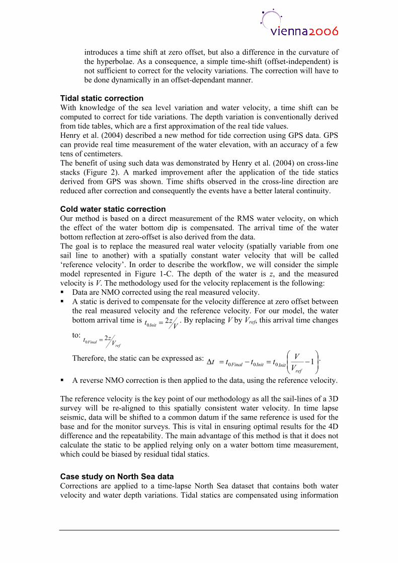
Introduction The level of the ocean as well as its physical properties varies with tides, currents or seasonal changes. Tide variations will affect the water depth, whereas changes in salinity or temperature will result in a change of seismic velocity. As marine data are acquired as a group of independent sail-lines that can be shot days or even months apart, water layer variations can induce lateral discontinuities (or jitters) on cross-line sections or on 3D CDP gathers which can lead to stack deterioration. These effects can be important, as stated by Wombell (1997) who observed, in West of Shetland data, time shifts up to 10-30 ms because of variations in water velocity. These lateral discontinuities can lead to more problems in 4D processing where mis-timing is observed between surveys, resulting in low repeatability. Tidal statics can be compensated using tide tables. Even though the accuracy of the tide tables, often defined far from the acquisition area, can be questioned, they give a first approximation for the static correction. It is a separate matter when we consider time shifts relating to velocity variations (often called cold water statics). Some methods have been proposed (Xu and Pham (2003), Fried and MacKay (2002)), but it stays a difficult problem and even today it is often tackled manually, leading to a time consuming and expensive process. The goal of this paper is to present a review of some methodologies available for water layer variation correction that can be used in 3D as well as in 4D. We will come back on the methodology presented by Henry et al. (2004) for tidal statics correction and will introduce a new workflow for velocity variation correction.

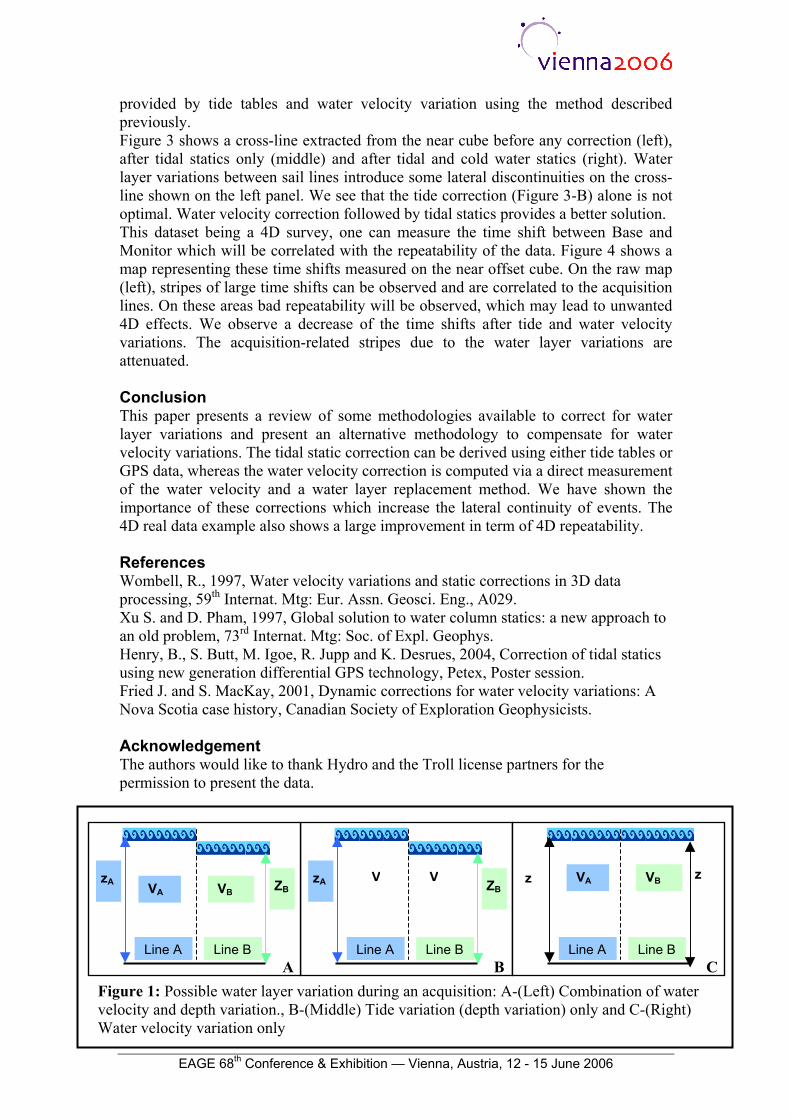
Theory for water layer variations We consider a simple model with a horizontal water bottom (Figure 1). Two sail-lines (A and B) have been acquired a few months apart. In the most general case, both the sea level and the water velocity have changed (Figure 1-A). For an offset x, the arrival time of the water bottom will follow the equations:

2222

02)(

+

=

+=

AAA

AAA V

xV

zVxtxt for sail line A

and 222

20

2)(

+

=

+=

BBB

BBB V

xV

zVxtxt for sail line B,

where z is the water bottom depth and V the water velocity. The combination of the two effects (depth and velocity variations) will result in a difference in the curvature of the hyperbolae of the water bottom reflection, but also in the water bottom arrival time at zero-offset. From these equations, we can conclude that it is impossible to differentiate between the two kinds of statics. Two particular cases can be identified: The velocity of the water has not changed with time (VA=VB=V, see Figure 1-

B) and only tidal statics (depth variation) affect the data. The curvature of the hyperbolae are the same, but t0 is different. Tidal statics can be corrected by applying a simple time shift on NMO corrected data, as long as the water depth variation is known accurately.

The depth of the water has not changed (zA=zB=z, see Figure 1-C) and only water velocity variations have an effect on the data. The change in velocity

introduces a time shift at zero offset, but also a difference in the curvature of the hyperbolae. As a consequence, a simple time-shift (offset-independent) is not sufficient to correct for the velocity variations. The correction will have to be done dynamically in an offset-dependant manner.

Tidal static correction With knowledge of the sea level variation and water velocity, a time shift can be computed to correct for tide variations. The depth variation is conventionally derived from tide tables, which are a first approximation of the real tide values. Henry et al. (2004) described a new method for tide correction using GPS data. GPS can provide real time measurement of the water elevation, with an accuracy of a few tens of centimeters. The benefit of using such data was demonstrated by Henry et al. (2004) on cross-line stacks (Figure 2). A marked improvement after the application of the tide statics derived from GPS was shown. Time shifts observed in the cross-line direction are reduced after correction and consequently the events have a better lateral continuity. Cold water static correction Our method is based on a direct measurement of the RMS water velocity, on which the effect of the water bottom dip is compensated. The arrival time of the water bottom reflection at zero-offset is also derived from the data. The goal is to replace the measured real water velocity (spatially variable from one sail line to another) with a spatially constant water velocity that will be called ‘reference velocity’. In order to describe the workflow, we will consider the simple model represented in Figure 1-C. The depth of the water is z, and the measured velocity is V. The methodology used for the velocity replacement is the following: Data are NMO corrected using the real measured velocity. A static is derived to compensate for the velocity difference at zero offset between

the real measured velocity and the reference velocity. For our model, the water bottom arrival time is

Vzt Init 2

0 = . By replacing V by Vref, this arrival time changes

to: ref

Final Vzt 2

0 =

Therefore, the static can be expressed as:

−=−=∆ 1000

refInitInitFinal V

Vtttt .

A reverse NMO correction is then applied to the data, using the reference velocity. The reference velocity is the key point of our methodology as all the sail-lines of a 3D survey will be re-aligned to this spatially consistent water velocity. In time lapse seismic, data will be shifted to a common datum if the same reference is used for the base and for the monitor surveys. This is vital in ensuring optimal results for the 4D difference and the repeatability. The main advantage of this method is that it does not calculate the static to be applied relying only on a water bottom time measurement, which could be biased by residual tidal statics.

Case study on North Sea data Corrections are applied to a time-lapse North Sea dataset that contains both water velocity and water depth variations. Tidal statics are compensated using information

EAGE 68th Conference & Exhibition — Vienna, Austria, 12 - 15 June 2006

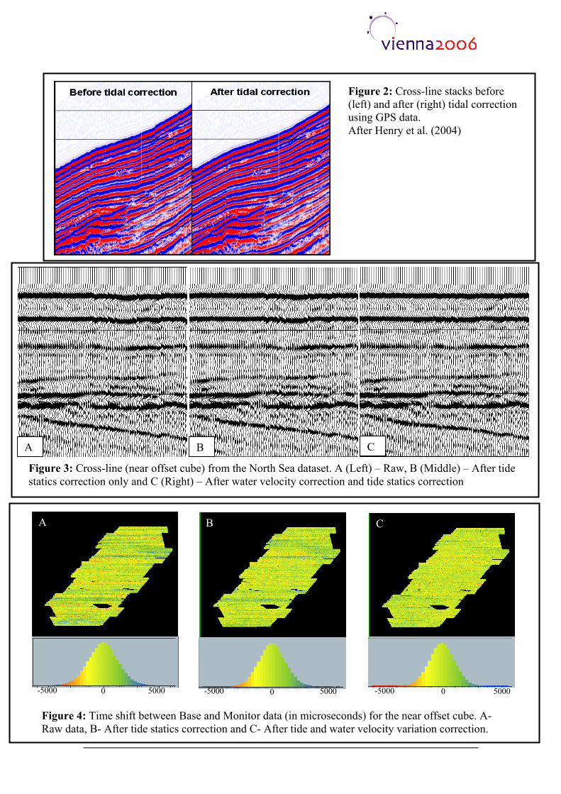
provided by tide tables and water velocity variation using the method described previously. Figure 3 shows a cross-line extracted from the near cube before any correction (left), after tidal statics only (middle) and after tidal and cold water statics (right). Water layer variations between sail lines introduce some lateral discontinuities on the cross-line shown on the left panel. We see that the tide correction (Figure 3-B) alone is not optimal. Water velocity correction followed by tidal statics provides a better solution. This dataset being a 4D survey, one can measure the time shift between Base and Monitor which will be correlated with the repeatability of the data. Figure 4 shows a map representing these time shifts measured on the near offset cube. On the raw map (left), stripes of large time shifts can be observed and are correlated to the acquisition lines. On these areas bad repeatability will be observed, which may lead to unwanted 4D effects. We observe a decrease of the time shifts after tide and water velocity variations. The acquisition-related stripes due to the water layer variations are attenuated. Conclusion This paper presents a review of some methodologies available to correct for water layer variations and present an alternative methodology to compensate for water velocity variations. The tidal static correction can be derived using either tide tables or GPS data, whereas the water velocity correction is computed via a direct measurement of the water velocity and a water layer replacement method. We have shown the importance of these corrections which increase the lateral continuity of events. The 4D real data example also shows a large improvement in term of 4D repeatability. References Wombell, R., 1997, Water velocity variations and static corrections in 3D data processing, 59th Internat. Mtg: Eur. Assn. Geosci. Eng., A029. Xu S. and D. Pham, 1997, Global solution to water column statics: a new approach to an old problem, 73rd Internat. Mtg: Soc. of Expl. Geophys. Henry, B., S. Butt, M. Igoe, R. Jupp and K. Desrues, 2004, Correction of tidal statics using new generation differential GPS technology, Petex, Poster session. Fried J. and S. MacKay, 2001, Dynamic corrections for water velocity variations: A Nova Scotia case history, Canadian Society of Exploration Geophysicists. Acknowledgement The authors would like to thank Hydro and the Troll license partners for the permission to present the data. Figure 1: Possible water layer variation during an acquisition: A-(Left) Combination of water

velocity and depth variation., B-(Middle) Tide variation (depth variation) only and C-(Right) Water velocity variation only

VzA V ZB

Line A Line BB

V z V

Line A Line B

VA VB z

C

VA zA VB ZB

Line A Line B A

-5000 5000 -5000 5000 -5000 5000 0 0 0

A B C

Figure 4: Time shift between Base and Monitor data (in microseconds) for the near offset cube. A-Raw data, B- After tide statics correction and C- After tide and water velocity variation correction.

Figure 3: Cross-line (near offset cube) from the North Sea dataset. A (Left) – Raw, B (Middle) – After tide statics correction only and C (Right) – After water velocity correction and tide statics correction

A B C

Figure 2: Cross-line stacks before (left) and after (right) tidal correction using GPS data. After Henry et al. (2004)