1  

Corporate investment and expropriation by controlling shareholders:

Evidence from Chinese listed companies1

Jinqing Zhang

Institute of Financial Studies Fudan University

Shanghai, China 200433

Hui Chen Institute of Financial Studies

Fudan University Shanghai, China 200433

Yunbi An

Odette School of Business University of Windsor

Windsor, Ontario, Canada N9B 3P4

Abstract

This paper presents a dynamic model that establishes the relationship between corporate investment and expropriation by controlling shareholders for firms facing different financing constraints. Using data on Chinese listed companies, we empirically test the model’s predictions about the effects of expropriation on inefficient investment in various periods. We find that firms with less tight financing constraints overinvest in the pre-expropriation period if the intended expropriation level is lower than a threshold, but underinvest if the expropriation level exceeds the threshold. However, expropriation does not impact inefficient investment in the expropriation and post-expropriation periods, even after the sanctions on these firms for expropriation are imposed. For firms with tight financing constraints, while expropriation does not significantly impact inefficient investment in the pre-expropriation period, it further tightens firms’ financing constraints in the expropriation and post-expropriation periods, leading to underinvestment. Moreover, investment is reduced after the sanctions on firms for expropriation are imposed and announced to the public.

Keywords: inefficient investment; controlling shareholder; tunneling JEL Classification: G31; G32; G34

                                                            1 This research was supported by the National Nature Science Funds of China (71073025 and 71471043), as well as the Competitive Guiding Project for the Plan of Promoting Innovation Abilities of Shanghai’s Universities and Colleges. An acknowledges the support from the Odette School of Business at the University of Windsor.

2  

1. Introduction

It is observed that in most countries corporate ownership is concentrated rather than widely

dispersed with control of most firms in the hands of controlling shareholders, who often are firms’

founding members and are entrenched (La Porta et al., 1999). As pointed out by La Porta et al.

(2002), controlling shareholders have the incentive and power to extract gains from minority

shareholders, a phenomenon referred to as expropriation or tunneling (Aslan and Kumar, 2012;

Johnson et al., 2000).2 Tunneling is a manifestation of the agency problems described by Jensen

and Meckling (1976), and can take a variety of forms, such as outright theft or fraud, transfer of

corporate funds and assets through self-dealing transactions, inside trading, as well as investor

dilution, to name just a few. Tunneling is particularly pronounced in China, given the highly

concentrated ownership structure and lack of a sound corporate governance mechanism in most

Chinese listed firms. For instance, from 2003 to 2013, the China Securities Regulatory

Commission (CSRC) as well as the Shanghai Stock Exchange (SSE) and the Shenzhen Stock

Exchange (SZSE) investigated and punished 451 instances of expropriation, involving an amount

of RMB 144.53 billion (approximately US $23.3 billion) and 423 listed companies.3 Tunneling

by controlling shareholders leads to a great variation in investment in these firms. In this paper

we are interested in exploring how corporate investment decisions are distorted as a result of

tunneling or intention to tunnel by controlling shareholders in listed firms.

As is well known, corporations select an investment level to maximize firm value under

perfect market assumptions (Hayashi, 1982). However, in reality, a corporation’s investment is

largely distinct from this optimal level due to market imperfections, such as information

asymmetries and agency problems (Aggarwal and Samwick, 2006; Bertrand and Mullainathan,

                                                            2 The terms expropriation and tunneling are used interchangeably in this paper. 3 Source: CSMAR database.

3  

2003; Hart and Moore, 1995; Stulz, 1990), resulting in either over- or underinvestment (referred

to as inefficient investment).4 For example, Myers and Majluf (1984) document that in the

presence of asymmetric information, firms may forgo valuable investment opportunities, leading

to underinvestment. Some recent studies in this area shed light on the relation between inefficient

investment and expropriation by controlling shareholders by empirically examining how the

ownership structure, the degree of separation of ownership and control, and the quality of

corporate governance impact corporate investment decisions, but report conflicting results. For

example, some work finds that tunneling by controlling shareholders in listed firms boosts the

cost of external financing (Aslan and Kumar, 2012; Gilson, 2006; Jiang et al., 2010; Johnson et

al., 2000), which negatively impacts firm investment. Bertrand and Mullainathan (2003) and

Giroud and Mueller (2010) document that firms with poor corporate governance tend to

underinvest.

On the other hand, Wu and Wang (2005) find that firms may have incentives to overinvest in

order to obtain large private benefits of control. Lan and Wang (2003) share a similar view, and

regard both diverting cash away from firms and overinvesting as two ways used by controlling

shareholders to pursue private benefits. Billett et al. (2011) and Albuquerque and Wang (2008)

find that firms with poor investor protection and corporate governance are likely to overinvest.

While it is widely documented in the literature that inefficient investment serves as a channel

for the controlling shareholder in a firm to pursue her own private benefits, the intertemporal

implications of tunneling for investment have not been formally analyzed either theoretically or

empirically. In contrast with previous studies, this paper proposes a three-period model to

explore a corporation’s investment behavior not only at the time when expropriation occurs but

                                                            4 Over- and underinvestment is inefficient, as they reduce a firm’s value. In practice, inefficient investment may be caused by many factors; expropriation is one of them.

4  

also before and after the expropriation date. In particular, we intend to derive an explicit relation

between firms’ inefficient investment and the fraction of output expropriated by controlling

shareholders in three different periods: pre-expropriation, expropriation, and post-expropriation.

Investment decisions may be distorted intertemporally as a result of expropriation or the

intention to expropriate in the future. In the pre-expropriation period, firms’ investment depends

not only on investment opportunities, but also on how investment impacts future tunneling

benefits and costs. In the expropriation period, tunneling reduces internal funds available for

investment, which in turn impacts firm investment and financing behavior, while in the post-

expropriation period, firms will have to bear the high external financing cost as a consequence of

tunneling practices, and invest accordingly. In addition, the impacts of tunneling on investment

depend critically on the tightness of financing constraints faced by the firms. By incorporating an

additional cost for external financing into the model, we are able to explain the heterogeneity of

investment behavior for firms facing different financing constraints. Our model can help us

better understand how and why tunneling impacts a firm’s dynamic investment decision as well

as the consequence of tunneling practices. This explains why the previous research on inefficient

investment and expropriation provides conflicting findings.

Using the data on Chinese listed firms, we empirically test various hypotheses regarding

inefficient investment and tunneling that are developed based on our model. To this end,

following Richardson (2006), we measure inefficient investment as the difference between a

firm’s total investment and its expected investment in a particular year. We adopt the difference-

in-differences method (Ashenfelter and Card, 1985) to examine how inefficient investment is

related to tunneling in various periods. Specifically, we classify firms into two groups: those with

and without tunneling activities, and then compare the inefficient investments in the two groups

5  

to gauge the tunneling effect. To address the endogenous problem due to observable variables,

we use the propensity score matching method to pair firms with and without tunneling activities

(Rosenbaum and Rubin, 1983). In contrast with the event study method used in most previous

studies (McNichols and Stubben, 2008), the difference-in-differences method is able to correct

for sample selection biases (Heckman, 1979) by isolating the tunneling effect from the effects of

other factors on inefficient investment.

Our research also adds to the literature on the relation between corporate ownership structure

and firm value. Previous studies on this subject generally highlight both the positive and negative

effects of managerial ownership on valuation of firms (Morck et al., 1988). On one hand, a larger

ownership of a firm held by its controlling shareholder helps diminish the incentives of the

firm’s controlling shareholder to expropriate other investors, and thereby is associated with

higher valuation (Jensen and Meckling, 1976). This is supported by the empirical evidence of

higher valuation in firms with higher cash-flow ownership by controlling shareholders (La Porta

et al., 2002). On the other hand, stronger entrepreneurial control adversely affects valuation

(Claessens et al., 2002). Our focus is on the firms’ distorted investment decisions as a result of

expropriation that is caused by the divergence of control rights and cash flow rights, which in

return translates into a reduced firm value.

We find that firms with less tight financing constraints overinvest in the pre-expropriation

period if the intended expropriation level in the future is lower than a threshold, but underinvest

if the intended expropriation level exceeds the threshold. However, expropriation does not

impact inefficient investment in the expropriation and post-expropriation periods for this type of

firms. For the firm with tight financing constraints, while our model predicts that expropriation

leads to a reduction in investment even underinvestment in the pre-expropriation period, our

6  

empirical results do not provide evidence in support of this prediction due to the fact that the

financing constraints faced by most Chinese listed firms are typically not sufficiently tight. In

addition, we show that expropriation leads to underinvestment in the expropriation and post-

expropriation periods for firms with relatively tight financing constraints, and investment is

further reduced after the sanctions on firms for expropriation are imposed and announced to the

public.

The remainder of this paper is organized as follows. Section 2 presents the model and

characterizes a firm’s dynamic investment behavior due to expropriation by the controlling

shareholder. Section 3 describes the research methodology. Section 4 discusses the data used in

this study. Section 5 analyzes the empirical results. Section 6 provides robustness tests, while

Section 7 concludes the paper.

2. The model

2.1. The model

Consider a firm that is fully controlled by a single major shareholder, referred to in this paper

as the controlling shareholder, who has cash-flow or equity ownership in the firm. The

controlling shareholder exerts her control by owning a large fraction of the firm’s voting rights,

which is higher than the fraction of cash-flow rights (La Porta et al., 1999). We assume that the

controlling shareholder is the manager.

There are four dates, t = 1, 2, 3, and 4, which define three periods: period i from date i to i+1

(i=1, 2, and 3). During period 1, the controlling shareholder has the intention to expropriate

minority shareholders, but has not taken any actions yet. During period 2, the controlling

shareholder is expropriating minority shareholders to obtain private benefits of control, while

7  

period 3 is the post-expropriation period. Following the neoclassical investment modelling

approach, we further assume:

(1) The firm’s profits at date t is tt KK )( ( 4,3,2,1t ), where tK is the firm’s capital

level at the beginning of period t , and represents the capital return in the period.

(2) During period 2, the controlling shareholder diverts a fraction s of profits 2 to herself

2s . )1,0(s is referred to as the expropriation level. As pointed out by La Porta et al.

(2002), much of such diversion requires costly transactions. Following La Porta et al.

(2002), the cost of expropriation is specified as 22

2 2

1),( ssC , where is the

degree of shareholder protection in the country/region where the firm operates. Intuitively,

firms that operate under a more protective legal system pay a higher cost for

expropriating a given share of profits. In addition, consistent with the law of diminishing

productivity, the marginal cost of expropriation is assumed to be an increasing function

of the expropriation fraction s.

(3) Capital at the end of period t is equal to the capital at the beginning of the period plus

new investment tI , minus capital depreciation during the period. If the rate of

depreciation is , then we have ttt KIK )1(1 .

(4) New investment incurs costs of adjusting the firm’s capital stock, such as fees for

installing new equipment and training workers. In this paper, the adjustment cost is

assumed to be ttttt KKIKI 2)(2

),(

, where is the rate of investment cost and

0 .

8  

(5) New investment can be financed by internally-generated funds, which are the firm’s

after-tax profits after subtracting the expropriation amount. However, external financing

has to be obtained if ),()()1( ttttt KIIKs , where ts is the expropriation level at

date t , and 02 ss as well as 0431 sss . Thus, the amount of external financing

is given by )()1(),( tttttt KsKIIF . The cost of external financing is defined

as tttt

tt KKFKF 2)(2

),(

, where t is the rate of financing cost and 0t .

The controlling shareholder/manager selects the amount of investment in each period to

maximize her private benefits:

22111111,,,

)()1(),(),()()(max321

IKsRKFKIIKUEsIII

))(,()(),(),( 222222 KsCKsKFKI

),(),()( 3333332 KFKIIKR

))1()( 443 KKR , (1)

S.t.

ttt KIK )1(1 ,

0)()1(),( ,0

0)()1(),( ),()1(),(

ttttt

ttttttttttt KsKII

KsKIIKsKIIF ,

where R is the discount factor.

If the manager acts in the best interest of all shareholders, no expropriation occurs and the

investment decision is determined by maximizing the firm value:

),(),()(),(),()()(max 222222111111,, 321

KFKIIKRKFKIIKUEIII

),(),()( 3333332 KFKIIKR

9  

))1()( 443 KKR , (2)

S.t.

ttt KIK )1(1 ,

0)(),( ,0

0)(),( ),(),(

tttt

ttttttttt KKII

KKIIKKIIF .

Apparently, the investment decisions based on model (1) could be substantially different from

the decisions based on model (2), giving rise to inefficient investment. Our model also indicates

that the distorted investment decision as a consequence of tunneling or intention of tunneling by

the control shareholder reduces firm value. This represents an additional cost to minority

shareholders in addition to the portion of profits expropriated by the controlling shareholder.

Chirinko and Schaller (2004) document that for firms with serious cash flow agency problems

(Jensen, 1986), corporate decisions are based on the lower executives’ expected return as

opposed to the shareholders’ return. However, in our setting, the distorted investment decisions

are an outcome of the controlling shareholder’s attempt (or practice) to expropriate minority

shareholders, and are not due to the lower discount rate used by the controlling shareholder.

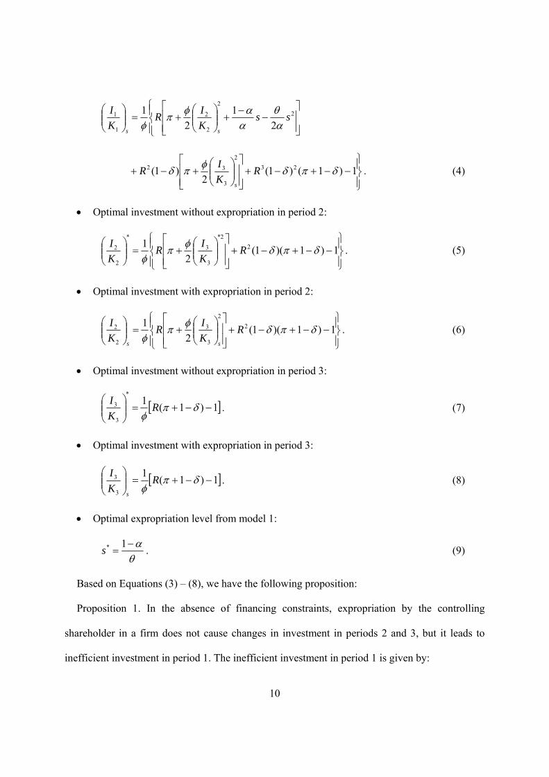
2.2. Corporate investment and expropriation in the absence of financing constraints

If a firm faces no financing constrains, i.e., 0t , then the optimal investment levels with

and without tunneling in each period can be solved from models 1 and 2:

Optimal investment without expropriation in period 1:

1)1()1(

2)1(

2

1 23

2*

3

32

2*

2

2

*

1

1

RK

IR

K

IR

K

I. (3)

Optimal investment with expropriation in period 1:

10  

2

2

2

2

1

1

2

1

2

1ss

K

IR

K

I

ss

1)1()1(

2)1( 23

2

3

32 RK

IR

s

.  (4)

Optimal investment without expropriation in period 2:

1)1)(1(

2

1 2

2*

3

3

*

2

2

RK

IR

K

I. (5)

Optimal investment with expropriation in period 2:

1)1)(1(

2

1 2

2

3

3

2

2

RK

IR

K

I

ss

. (6)

Optimal investment without expropriation in period 3:

1)1(1

*

3

3

R

K

I. (7)

Optimal investment with expropriation in period 3:

1)1(1

3

3

R

K

I

s

. (8)

Optimal expropriation level from model 1:

1*s . (9)

Based on Equations (3) – (8), we have the following proposition:

Proposition 1. In the absence of financing constraints, expropriation by the controlling

shareholder in a firm does not cause changes in investment in periods 2 and 3, but it leads to

inefficient investment in period 1. The inefficient investment in period 1 is given by:

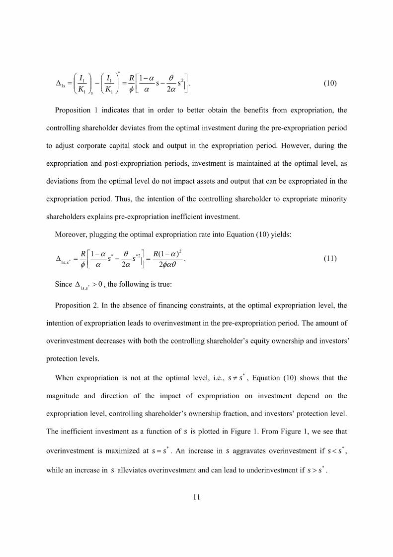
11  

2

*

1

1

1

11 2

1ss

R

K

I

K

I

s

s

. (10)

Proposition 1 indicates that in order to better obtain the benefits from expropriation, the

controlling shareholder deviates from the optimal investment during the pre-expropriation period

to adjust corporate capital stock and output in the expropriation period. However, during the

expropriation and post-expropriation periods, investment is maintained at the optimal level, as

deviations from the optimal level do not impact assets and output that can be expropriated in the

expropriation period. Thus, the intention of the controlling shareholder to expropriate minority

shareholders explains pre-expropriation inefficient investment.

Moreover, plugging the optimal expropriation rate into Equation (10) yields:

2

)1(

2

1 22**

,1 *

R

ssR

ss. (11)

Since 0*,1

ss, the following is true:

Proposition 2. In the absence of financing constraints, at the optimal expropriation level, the

intention of expropriation leads to overinvestment in the pre-expropriation period. The amount of

overinvestment decreases with both the controlling shareholder’s equity ownership and investors’

protection levels.

When expropriation is not at the optimal level, i.e., *ss , Equation (10) shows that the

magnitude and direction of the impact of expropriation on investment depend on the

expropriation level, controlling shareholder’s ownership fraction, and investors’ protection level.

The inefficient investment as a function of s is plotted in Figure 1. From Figure 1, we see that

overinvestment is maximized at *ss . An increase in s aggravates overinvestment if *ss ,

while an increase in s alleviates overinvestment and can lead to underinvestment if *ss .

12  

Proposition 3. In the case where 5.0* s , for any expropriation level )1,0(s , the inefficient

investment 0 s , and the intention of expropriation always causes overinvestment in period 1.

In the case where 5.0* s , if the expropriation level )2~,0( *sss , then the inefficient

investment 0 s , and the intention of expropriation causes overinvestment. If the expropriation

level )1,~(ss , then the inefficient investment 0 s , and expropriation causes underinvestment.

The optimal expropriation level *s is negatively related to both the investors’ protection and

the controlling shareholder ownership levels, indicating that better investor protection or high

cash flow ownership helps reduce expropriation. If both the investors’ protection and controlling

shareholder ownership levels are relatively low, *s can be higher than 0.5. Proposition 3 implies

that expropriation always leads to overinvestment in the pre-expropriation period for relatively

low investors’ protection and controlling shareholder ownership levels. For firms with better

investor protection and higher controlling shareholder equity ownership, *s can be lower than

0.5. In this case, either overinvestment or underinvestment can occur, depending on whether or

not the expropriation level exceeds a threshold. Namely, if expropriation is less than the

threshold s~ , expropriation causes overinvestment. However, if expropriation exceeds the

threshold s~ , expropriation leads to underinvestment.

Note that the threshold level falls as the investor protection level and controlling shareholder

equity ownership rise. Thus, Proposition 3 also says that firms with better investor protection and

higher controlling shareholder equity ownership are more likely to underinvest in the pre-

expropriation period than other firms.

For Chinese listed companies, Jiang et al. (2010) find that the controlling shareholders’

average expropriation level can be appropriately measured by other receivables as a percentage

13  

of total assets (ORECTA). We find that the average ORECTA is 0.051 for all firms during our

sample period 2003-2013, which is close to the optimal expropriation level according to the law

of large numbers. Given that this is far below 0.5, there is a threshold expropriation level in

Chinese listed firms above which firms will underinvest. Motivated by short-term benefits,

expropriation by controlling shareholders in Chinese listed firms may be well above the optimal

expropriation level, leading to underinvestment at the pre-expropriation period.

2.3. Corporate investment and expropriation in the presence of financing constraints

The previous analysis ignores the additional cost of external financing. However, in the real

world, it is costly for a firm to raise external funds due to information asymmetry between inside

and outside investors. This financing constraint may impact the relation between firm investment

and expropriation. In this section, we assume a non-zero external financing cost, i.e., 0t , and

characterize the relation between inefficient investment and expropriation. For convenience, we

analyze the investment decisions in reverse order.

2.3.1. Firm investment in the post-expropriation period

Aslan and Kumar (2012) find that expropriation or tunneling raises firms’ cost of debt

financing. For this reason, we assume that the post-expropriation cost of financing s,3 is higher

than the cost of financing without tunneling 3 . Based on Equations (1) and (2), the optimal

investment levels with tunneling fsKI ,33 )( and without tunneling *33 )/( fKI in period 3 are,

respectively, given by:

1

)(1

)1(

,3

3,3

,3

3

fssfs

K

F

R

K

I, (12)

14  

1

)(1

)1(

*

3

33

*

3

3

ff

K

F

R

K

I. (13)

Proposition 4. In the presence of financing constraints, expropriation leads to underinvestment

in the post-expropriation period, which is given as:

)(])(1[

)(

3,32*

3

33

*

3

3*

3

3

,3

3,3

s

f

f

ffs

f

K

FK

FR

K

I

K

I. (14)

Proposition 4 reveals that firms underinvest in the post-expropriation period due to the fact

that expropriation tightens corporate financing constraints. Note that one implicit assumption in

Proposition 4 is that tunneling does not affect internally-generated funds in a firm in the post-

expropriation period. In fact, tunneling usually reduces the firm’s internal funds in the post-

expropriation period, boosting the demand for corporate financing, i.e., *33,33 )/()/( ffs KFKF .

In this case, even if financing costs remain unchanged after tunneling ( 3,3 s ), we still have

*33,33 )/()/( ffs KIKI , and tunneling leads to underinvestment in the post-expropriation period.

For example, the controlling shareholder of Jiugui Liquor Co. engaged in tunneling activities in

years 2003-2005. As a result, the firm’s monetary capital scaled by total assets was particularly

low for the following four consecutive years with an average of 0.06, and it gradually increased

to 0.15 and 0.43 in 2010 and 2011, respectively.5

2.3.2. Corporate investment and expropriation in the expropriation period

Solving Problems (1) and (2) yields the following optimal expropriation fraction, optimal

investments with tunneling and without tunneling in period 2:

                                                            5 Sources: CSMAR database.

15  

fsf K

Fs ,

2

22* )(1

, (15)

1

)(1

)]1)(1([

,2

22

,2

,2

2

fs

fs

fs

K

F

RGR

K

I, (16)

1

)(1

)]1)(1([

*

2

22

*2

*

2

2

f

f

f

KF

RGR

K

I, (17)

where )/()/(2

)/)](/(1[2 333

233

32333332 KFKFKIKFG

, representing the reduction

in the investment and financing costs in period 3 for one unit increase in investment in period 2.

Taking the partial derivative of fsKI ,22 )/( with respect to s yields:

0

)(

)(1

)]1)(1([

)(1

,2

2

2

,2

22

,2,2

,2

22

,2

2

s

K

F

K

F

RGR

s

G

K

F

R

s

K

Ifs

fs

fsfs

fs

fs

.

(18)

Further, using the Taylor’s formula, we can obtain the inefficient investment in period 2:

0

0

,2

2*

2

2

,2

2,2

ss

K

I

K

I

K

I

s

fs

ffs

f . (19)

Proposition 5. In the presence of financing constraints, expropriation leads to underinvestment

in the expropriation period. In addition, an increase in the expropriation level exacerbates

underinvestment.

16  

Intuitively, tunneling by the controlling shareholder decreases the internal funds available for

investment, thereby increasing the demand for external corporate financing. This will boost the

cost of financing, and thus discourage investment.

2.3.3. Corporate investment and expropriation in the pre-expropriation period

Similarly, the optimal investments in period 1 with and without intention of expropriation are

given as:

1

)(1

)]1()1(]2

1[

,1

11

232,1

,1

1

fs

fffs

fs

K

F

RssGR

K

I, (20)

1

)(1

)]1()1()(

*

1

11

23*1

*

1

1

f

f

f

K

F

RGR

K

I, (21)

where 22222

2222

222221 )1()/()/(2

)/)](/(1[2

GRKFKFKIKFG , representing

the reduction in investment and financing costs in periods 2 and 3 for one unit increase in

investment in period 1.

Based on Equations (20) and (21), the inefficient investment in period 1 is given by:

2*

1,1

1

11

*

1

1

,1

1,1 2

1

)](1[ffffs

ffs

f ssGG

K

FR

K

I

K

I

MNss

K

FR

ff2

22

1

11

22)](1[

, (22)

where

17  

1*

2

2

,2

22

2*

2

2

2

,2

22

ffsffsK

I

K

I

K

I

K

IN , (23)

3*

2

2

3

,2

2

4*

2

2

4

,2

22

8

3

ffsffsK

I

K

I

K

I

K

IM

*2,2

*

2

2

,2

2

2

2ffs

ffs

GGK

I

K

I

. (24)

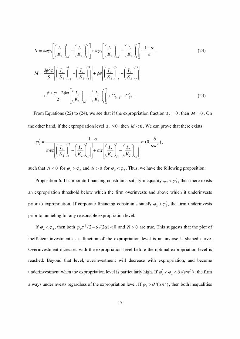
From Equations (22) to (24), we see that if the expropriation fraction 0fs , then 0M . On

the other hand, if the expropriation level 0fs , then 0M . We can prove that there exists

),0(1

2

,2

2

*

2

2

2

,2

2

2*

2

2

'2

fsffsfK

I

K

I

K

I

K

I,

such that 0N for '22 and 0N for '

22 . Thus, we have the following proposition:

Proposition 6. If corporate financing constraints satisfy inequality '22 , then there exists

an expropriation threshold below which the firm overinvests and above which it underinvests

prior to expropriation. If corporate financing constraints satisfy '22 , the firm underinvests

prior to tunneling for any reasonable expropriation level.

If '22 , then both 0)2/(2/2

2 and 0N are true. This suggests that the plot of

inefficient investment as a function of the expropriation level is an inverse U-shaped curve.

Overinvestment increases with the expropriation level before the optimal expropriation level is

reached. Beyond that level, overinvestment will decrease with expropriation, and become

underinvestment when the expropriation level is particularly high. If )/( 22

'2 , the firm

always underinvests regardless of the expropriation level. If )/( 22 , then both inequalities

18  

0)2/(2/22 and 0N hold. This suggests that the plot of inefficient investment as a

function of the expropriation level is a U-shaped curve. The inefficient investment decreases,

reaches its minimum value, and then increases as the expropriation level increases. In this case,

the inefficient investment is negative for a reasonable expropriation level, which implies

underinvestment.

Proposition 6 says that in the presence of corporate financing constraints, the threshold effect

becomes less pronounced as financing constraints tighten: firms facing a particularly tight

financing constraint tend to underinvest prior to tunneling.

Our model provides a number of testable predictions with respect to the relationship between

inefficient investment and expropriation for firms with different financing constraints. Note that,

in reality, financing constraints are present in all firms, though the tightness of financing

constraints varies across firms. To summarize, the following testable hypothesis are derived from

our model:

H1. For companies with less tight financing constraints, expropriation leads to

overinvestment in the pre-expropriation period if the intended expropriation level is lower than a

threshold, while it leads to underinvestment if the intended expropriation level is greater than the

threshold.

H2. For companies with tight financing constraints, expropriation leads to underinvestment

in the pre-expropriation period, regardless of the severity of expropriation.

H3. For companies with financing constraints, expropriation leads to underinvestment in

both the expropriation and post-expropriation periods, and this effect becomes more pronounced

as the tightness of financing constraints increases.

19  

In the remainder of this article, we will empirically test these hypotheses using data on

Chinese listed companies. To this end, we focus on tunneling activities such as outright theft,

connected transactions, connected loans, and transfer pricing based on the CSRC and exchange

administrative sanction decisions. We define the expropriate period as the year in which

tunneling activities are conducted, while pre- and post-expropriate periods are one year prior to

and the first two years after the expropriation year, respectively.6 Importantly, we will also

examine how inefficient investment changes after the administrative sanctions against firms or

their executives for tunneling activities are imposed and announced to the public.

3. Research methodology

3.1. Measuring inefficient investment

Following Richardson (2006), we decompose a firm’s net investment into its expected

investment and inefficient investment, where the former is determined by the firm’s growth

opportunities and financing constraints. To estimate inefficient investment, we run the following

regression:

1,51,41,31,21,10, titititititi SizeAgeCashLevGrowthI

tik

ktik

ttittiti INDUSTRYYEARIAR ,1,1,1,71,6 , (25)

where the explained variable Ii,t is the new investment level in firm i in year t as a percentage of

year-end assets. The major explanatory variable in the regression is Growthi,t-1, which is Tobin’s

Q for firm i in year t – 1 as a measure of investment opportunities. The control variables include

Levi,t-1, Cashi,t-1, Agei,t-1, Sizei,t-1, ARi,t-1, and Ii,t-1, which are the firm’s financial leverage

measured by the ratio of total assets to total liabilities, cash balance scaled by total assets, firm

                                                            6 Our empirical results show that the impact of tunneling on investment prior to the tunneling year is generally less than 2 years, and the impact after the tunneling year is generally less than 3 years. Figure 2 also shows that firm inefficient investment, size, debt and equity financing, free cash flow, and earnings per share vary greatly within this time period.

20  

age defined as the logarithm of the number of years since the firm was founded, firm size

measured by the logarithm of total assets, stock return, and total investment in the past year,

respectively. These control variables are present to control for firm characteristics that impact

expected investment. In addition, dummy variables YEAR and INDUSTRY are included to control

for the time and industry effects, respectively.

The fitted value from the regression represents the estimate of the expected new investment

for a firm in a particular year, and the residual is the estimate of inefficient investment (II). A

positive residual corresponds to overinvestment (OI), while a negative residual is associated with

underinvestment (UI).

3.2. Measuring the severity of tunneling

Our model shows that the expropriation level plays an important role in explaining whether

firms overinvest or underinvest in different periods. To examine this issue, we differentiate

severe tunneling from non-severe tunneling practices, based on the average ORECTA in listed

firms. ORECTA reflects the size of non-operating financial transactions between a company and

its controlling shareholder in a given year, and can be used to measure the severity of tunneling

(Jiang et al., 2010). In this paper, we first examine whether ORECTA observations fit the normal

distribution using the quantile-quantile normality test, and then identify those extreme values

with a confidence level higher than 95% for firms with reported tunneling practices.7 These

observations are considered to be associated with severe tunneling activities. We understand that

some tunneling practices may not be reflected in firms’ ORECTAs. Thus, we also use the type of

sanctions imposed by the CSRC to determine whether a tunneling activity is severe. In China,

companies or their top executives that have committed tunneling activities could be given a

                                                            7 This is consistent with the criterion used by large financial institutions such as Morgan Stanley to measure extreme events in risk management. The same criterion is also applied to the classification of the tightness of financing constraints.

21  

warning, imposed a penalty fine, given a circulated criticism, ordered to correct violations of

laws and regulations, or issued a public denouncement by the CSRC once their illegal conduct

has been investigated and confirmed. Of all these punishments, public denouncement represents

the most severe administrative sanction decision, often issued when illegal practices are judged

to be serious, based on the facts, nature and condition of, and the harmful effects caused by the

illegal conduct.

3.3. Measuring the tightness of financing constraints

Our model predicts that the way in which inefficient investment is related to tunneling

depends greatly on the tightness of a firm’s financing constraints. To test our hypotheses, we

classify firms as having either less tight or tight financing constraints, based on their banking

credit constraints. We focus on banking credit constraints, as bank loans are a major source of

external funds for Chinese listed companies (Cai et al., 2005; Li and Yu, 2009). Further, the

measures such as dividend payout, debt rating, commercial paper rating, and Kaplan-Zingales

Index used in previous studies (Almeida et al., 2004; Fazzari et al., 1988; Kaplan and Zinglales,

1997; Whited, 1992) cannot accurately measure the financing constraints faced by Chinese listed

companies. This is because the dividend policies of Chinese listed firms are largely affected by

economic policies. In addition, data on debt credit quality ratings are not readily available due to

the fact that the Chinese bond markets are underdeveloped and the credit quality ranking

mechanism in China is not well established (Wei and Liu, 2004; Wang, 2009)

During the period in which China’s bank financing system transitioned from a centrally-

planned to a market-oriented system, the Chinese state-owned banks made lending decisions

based not only on a firm’s profitability and capability of generating cash flows, but also on

political considerations. On one hand, as a result of market-oriented banking system reforms,

22  

Chinese state-owned banks now have strong incentives to maximize profitability while

controlling risk exposure, and thus are more willing to make loans to firms with high free cash

flows, well-known loan guarantors, and high value collaterals. On the other hand, the Chinese

banking system remains under control of governments, and is used to promote economic growth

and help implement the government’s economic policies. Given the particularly important role

that large SOEs play in the Chinese economy, Chinese banks are expected to support SOEs with

soft loans and other financial supports. Chinese SOEs are typically granted the privilege of

obtaining bank loans and other sources of financing at a low cost. Therefore, to determine

whether or not a firm faces tight financing constraints, we consider the following variables: net

operating cash flows, loan guarantors, total pledgeable assets, firm size, and whether the firm is a

SOE.

Firms with less tight financing constraints include those that are large SOEs, as well as those

with high net operating cash flows, better loan guarantors, and high value pledgeable assets.

More specifically, we first sort all listed companies in our sample based on firm size and define

the top 19.1% of the firms that are under government control as firms with less tight financing

constraints.8 Meanwhile, the following firms are also considered to be the firms with less tight

financing constraints: those whose net operating cash flows or net fixed assets are among the top

5% of all listed firms, or those that have central SOEs (SOEs under the supervision and

administration of the State-owned Assets Supervision and Administration Commission (SASAC)

                                                            8 Given that the golden ratio 0.618 represents beauty, harmony, and balance in physical form, we use the golden ratio to classify firms into different groups based on firm size. Namely, observations on firm asset values with confidence levels [0, 0.191), [0.191, 0.809], and (0.809, 1] are defined as small, medium, and large size firms, respectively.

23  

of the State Council) or large SOEs as their related parties.9 The rest of the firms are considered

to be firms with tight financing constraints.

3.4. Empirical models

In this paper we adopt the difference-in-differences (DID) method (Ashenfelter and Card,

1985) to assess the impact of tunneling by controlling shareholders on corporate investment

decisions. The DID method classifies the sample into a treatment group and a control group,

where the former consists of firms that engage in tunneling practices in period 2, and the latter

consists of firms without tunneling practices. Then, the difference in investment between the two

groups in each period is estimated and used to gauge the tunneling effect. Compared with the

event study method, this approach can isolate the tunneling effect from the impacts of other

factors that changed in the expropriation period.

3.4.1. Construction of the treatment and control groups

To obtain an unbiased estimate of the expropriation effects, the treatment and control groups

should be carefully constructed such that they are similar in terms of the observables other than

the impact of tunneling. More specifically, we select companies for the treatment and control

groups in order to ensure that both groups are similar in size, industry, and ownership structure,

among others apart from tunneling, and then compare their investment decisions. To this end, we

adopt the propensity score matching (PSM) method (Rosenbaum and Rubin, 1983), which pairs

treatment and control groups with similar values on the propensity score (PS) to correct for

sample selection biases due to observable differences between the two groups. The following

                                                            9 A related party is a legal entity or an individual who directly or indirectly controls the firm. We focus on related parties, as the primary loan guarantors for a Chinese firm are the firm’s related parties. We particularly focus on those that have related party transactions with their firms for at least 5 years and those with an averaged related party transaction value to total assets ratio higher than the overall average.

24  

describes the steps for constructing the treatment and control groups based on the PSM matching

procedure:

First, we identify the firms that have never engaged in tunneling activities, namely the

control firms. Given the illicit nature of tunneling, the controlling shareholders tend to cover up

tunneling practices to avoid being detected and punished by regulatory authorities and exchanges.

Thus, it is important to ensure that all the companies in the control group are truly those without

tunneling rather than those whose tunneling activities have not yet been revealed. In our paper a

company is classified as a “control” company if: 1) it has never been punished by the CSRC; 2)

it has never received any audit suggestions other than “with no reservation” in auditors’ reports;

3) it has never received a special treatment designation (ST) from CSRC;10 4) it has never been

involved in large non-operating fund transactions with its related parties. Precisely, the ORECTA

has never been higher than the 61.8th percentile of all listed companies.11

Second, we estimate all firms’ PSs. Following Deheji and Wahba (2002), we estimate a

firm’s PS using the Logit model as below:

tik

ktik

ttit

jti

jj

titi

titi INDUSTRYYEARInfInfVioP

InfVioP,,,,0

,,

,,

)|1(1

)|1(ln

, (26)

where Vioi,t is a dummy variable that equals 1 if firm i conducted tunneling activities in year t,

and equals 0 otherwise. jtiInf , represents the jth factor that influences tunneling for firm i in year t.

In this paper, following Zhang and Shi (2013) and Shi (2012), we consider the following three

types of factors. We consider factors that affect the opportunity cost of tunneling, including the

proportion of total shares held by major shareholders (Top1) and the firm’s growth opportunities

                                                            10 Gao and Song (2007) and Gao and Zhang (2009) find that the companies that have received audit suggestions other than “with no reservation” in auditor’s reports and those that have received a special treatment designation (ST) from CSRC are more likely to engage in tunneling practices. 11 The golden ratio is used to classify firms into high and low ORECTA firms. See Footnote 8 for explanation.

25  

measured by Tobin’s Q (Q). Next, we consider factors that affect investor protection level,

including the degree of separation between control rights and cash flow rights (Sep), the degree

of equity ownership concentration (Her), the proportion of outstanding shares of stock held by

institutional investors (Ins), the separation of CEO role from Board chair role (Dep), board size

(Board), the proportion of outside independent directors on the board of directors (Indp), agency

costs arising from conflicts of interest between the controlling shareholder and top executives

(AC), the proportion of total shares held by corporate executives (Gshare), degree of leverage

(Lev), whether firm i is audited by the Big Four accounting firms (Adu),12 whether the firm has

H-shares listed on the Hong Kong Stock Exchange (Ph), and whether the time of observation is

after January 1, 2006 on which date the new Company Law of the People’s Republic of China

became effective (Law). Finally, we consider factors that affect financing constraints, including

whether the firm is a large SOE or has central SOEs as loan guarantors (Gua), whether the firm

is a SOE (Sta), operating cash flows (Cf), value of fixed assets (Fix), and firm size (Size). Table 1

summarizes these variables and their definitions. To control for the possible non-linear effects of

agency costs and degree of leverage on tunneling, we include AC2 and Lev2. Given that the

impact of corporate governance on controlling shareholder tunneling may vary after the new

Company Law became effective on January 1, 2006, we also include cross-product terms

Ins×Law, Her×Law, Dep×Law, Board×Law, Indp×Law, and Gshare×Law. Based on the

regression results, we can obtain the expected probability of tunneling by the controlling

shareholder in a firm, which is the estimate of the firm’s PS.

  Third, we pair treated firms (firms with tunneling activities) and control firms (firms without

tunneling activities). Propensity score matching entails forming matched groups of treated and

control firms who share a similar value of the propensity score (Rosenbaum and Rubin, 1983).                                                             12 The world’s four largest accounting firms include Deloitte, PwC, Ernst & Young, and KPMG.

26  

Our empirical analysis shows that the time period for the controlling shareholder’s preparation

for tunneling is typically less than 2 years, and the impact of tunneling on firm investment lasts

less than 3 years. Thus, we match treated and control companies in terms of their propensity

scores achieved 2 years prior to the tunneling year, using the nearest neighbor matching

method.13 We also use the radius matching and kernel matching algorithms to test the robustness

of our results in this paper.

Finally, we compare the means of the explanatory variables for treated and control firms

within each subclass, and find that the differences are not significant. This indicates that our

selection method has taken into account the endogeneity of tunneling due to observables.

3.4.2. Test of endogeneity due to unobserved variables

While the PSM method addresses the endogenous problem due to observables, endogeneity

can occur if some unobserved variables that influence firm inefficient investment also influence

tunneling. If such unobserved variables exist, then the DID estimate of tunneling effect on

inefficient investment may not be consistent. To test this potential endogenous problem, we use a

Logit model to test whether firms’ inefficient investment (II) and the lagged inefficient

investment (L_II) affect tunneling activities by control shareholders. Intuitively, if some

unobservable variables that are associated with inefficient investment influence tunneling, then

the coefficients on both II and L_II will be significant. If otherwise, these coefficients are

insignificant. This Logit model is as follows:

jjjtiti

titi

titi ControlIILIIInfVioP

InfVioP ,2,10

,,

,, _)|1(1

)|1(ln

tik

kkt

tit INDUSTRYYEAR ,1, . (27)

                                                            13 We primarily use 2 years prior to expropriation as the base period in this exercise. For this purpose, we also use data from 2000 to 2002 to ensure that our sample is for the period from 2003 to 2013.

27  

where IIi,t is inefficient investment firm i in year t, which is the difference between firm i’s net

investment in year t and the industry average net investment, and L_IIi,t is one-year lagged IIi,t.

Controlj represent the control variables, which are the factors that affect inefficient investment

considered in Equation (26).

3.4.3. Inefficient investment and tunneling

To detect the impact of tunneling by the controlling shareholder on a firm’s dynamic

investment decisions, we run the following regression

tititititititi SafNafSmidNmidSbeNbeII ,6,5,4,3,2,10,  

      titititititititi xSmidxNmidxSbexNbe ,,4,,3,,2,,1

titititititi xxSafxNaf ,,7,,6,,5 ,           (28)

where IIi,t represents inefficient investment (over- or underinvestment) for firm i in year t

estimated from Equation (25). xi,t is a dummy variable taking the value 1 if firm i is in the

treatment group, and 0 if the firm is in the control group. Nbe, Nmid, and Naf are dummy

variables for the pre-expropriation, expropriation, post-expropriation periods, respectively, if a

tunneling activity is considered not severe, while Sbe, Smid, and Saf are dummy variables for the

pre-expropriation, expropriation, and post-expropriation periods, respectively, if a tunneling

activity is considered severe. No control variables are included in this model, as the relevant

effects are controlled when treated and control firms are matched. To test the robustness of the

results, we control for the average industry inefficient investment, time, and industry effects, and

run the following regression:

tititititititi SafNafSmidNmidSbeNbeII ,6,5,4,3,2,10,  

      titititititititi xSmidxNmidxSbexNbe ,,4,,3,,2,,1

28  

tititititi xxSafxNaf ,7,,6,,5

      tik

ktikti

ttti INDUSTRYYEARAII ,,,,8 ,       (29)

where AIIi,t represents the average inefficient investment for firm i’s industry in year t. YEAR and

INDUSTRY are the dummy variables aiming for controlling for the time and industry effects,

respectively.

Our interest is in the coefficients m ( 6,,2,1 m ) on the cross-product terms, which

reflect the impact of tunneling on inefficient investment in various periods. A significant and

positive estimated suggests that tunneling aggravates overinvestment or alleviates

underinvestment, while a significant and negative estimated suggests that tunneling alleviates

overinvestment or aggravates underinvestment during a particular period. More specifically, the

estimated 1 and 2 measure the impacts of non-severe and severe tunneling on pre-

expropriation inefficient investment, respectively. If Hypothesis 1 is true, then 1 is significantly

positive and 2 is significantly negative, when the data on companies with less tight financing

constraints is used in the estimation. If Hypothesis 2 is true, then both 1 and 2 are

significantly negative for companies with tight financing constraints. Similarly, if Hypothesis 3

is true, then the estimated 3 , 4 , 5 , and 6 are all significantly negative for firms with

financing constraints.

4. Data

Our sample period extends from January 2003 to December 2013. We start with all A-share

companies listed on the Shanghai and Shenzhen Stock Exchanges, which are the only two stock

exchanges in China. We exclude companies in the financial sector, companies with a post-IPO

period less than two years, as well as companies with missing or irregular data in our sample

29  

period. To prevent extreme observations from influencing our results, all of our variables are

winsorized at the 1st and 99th percentiles (Flannery and Rangan, 2006). We end up with a total

of 432 companies with 4406 observations. All financial data for these companies is obtained

from the CSMAR database, whereas the data on tunneling is manually collected from the

CSMAR and wind databases as well as from companies’ rectification reports.

Table 2 reports the results of Regression (25), which show that firms’ expected investment

are significantly positively related to firm growth opportunities, one-period lagged returns, cash

balance, firm size, and investments, but are significantly negatively related to firm financial

leverage and age. This finding is consistent with those in the previous studies on Chinese listed

companies (Du et al., 2011; Jiang et al., 2009; Wei and Liu, 2007; Xin et al., 2007). The

residuals are obtained accordingly, which are the estimates of inefficient investment.

Table 3 presents the descriptive statistics of inefficient investment and various major

variables considered in our model for companies with different financing constraints. We find

that while the average inefficient investment is negative for all companies and for companies

with tight financing constraints, it is positive for companies with less tight financing constraints.

In addition, companies with less tight financing constraints typically have a lower Tobin’s Q,

stock return, degree of separation of the CEO role from board chair role, and proportion of shares

held by corporate executives than companies with tight financing constraints, but have a higher

value of all other variables.

Panel A of Table 4 reports the descriptive statistics of inefficient investments for companies

with tunneling practices in pre-expropriation, expropriation, and post-expropriation periods,

while Panel B reports the descriptive statistics for companies without tunneling practices in the

corresponding periods. We note that all firms, on average, overinvest in the pre-expropriation

30  

period, but firms with tunneling activities overinvest more. In the expropriation and post-

expropriation periods, treated firms underinvest while control firms tend to overinvest. Moreover,

treated firms underinvest the most after the sanctions on firms for tunneling are imposed and

released to the public. Control firms’ overinvestment is more pronounced after the tunneling year.

This observation suggests that tunneling leads to overinvestment in the pre-expropriation period,

while it reduces investment and can lead to underinvestment in the expropriation and post-

expropriation periods.

Figure 2 displays firms’ new investment, size, financing, free cash flow, and earnings per

share (EPS) for companies with tunneling during various years before and after expropriation.

Given the relatively small number of observations on firms with less tight financing constraints

and severe tunneling activities, in this figure we focus only on those with tight financing

constraints and with non-severe tunneling activities. From this figure, we see that the average

new investment levels in the years prior to expropriation are all positive, and the average new

investment one year before expropriation is particularly higher than the average for the years

with no tunneling activities. However, the inefficient investments in the years prior to

expropriation are lower than the average for years other than the years considered in the figure.

This indicates that in the pre-expropriation period, while firms are prone to increase investment,

the average investment is lower than the optimal level. We also note that in the expropriation

year and years after expropriation, the averaged new investment level and inefficient investment

level are negative. In particular, in the first and second years after tunneling and in the first year

after the sanctions on firms for tunneling are imposed, the average new investment level is much

lower than the corresponding levels for the years with no tunneling activities. This demonstrates

that tunneling reduces investment in both expropriation and post-expropriation periods for these

31  

firms. This effect is especially pronounced in first year and second year after tunneling, as well

as in the year when sanctions are imposed and in the first year after sanctions are imposed.

This figure also indicates that in the pre-expropriation period, the average firm size and the

average sizes of both equity and debt financing are close to or higher than the averages for the

years other than the years before and after tunneling, but they decline dramatically in the

expropriation and post-expropriation periods. A similar pattern is also observed for free cash

flow and earnings per share in these firms. This suggests that tunneling tightens the financing

constraints and reduces the size of firm financing and investment, leading to a lower firm value.

5. Empirical results

5.1. Inefficient investment and expropriation

Table 5 reports the estimation results of Equation (27). Model 1 includes II as an explanatory

variable, whereas Model 2 includes both II and L_II. The estimated coefficients on II and L_II in

both models are not significant, indicating that inefficient investment does not significantly

impact controlling shareholder expropriation decisions. This confirms that there are no other

factors that influence both firm inefficient investment and or tunneling after controlling for the

effect of observables, and that the DID method can be used in our analysis.

Table 6 reports the results of Equations (28) and (29). We note that for firms with less tight

financing constraints, the estimated coefficient on Nbe×x is positive and significant at the 1%

level, whereas the coefficient on Sbe×x is negative and significant at the 5% level, regardless of

whether the average industry inefficient investment is controlled in the regression. This result

indicates that these firms overinvest in the pre-expropriation period if controlling shareholders

intend to engage in non-severe tunneling activities at a later date, but underinvest if controlling

shareholders intend to engage in severe tunneling activities. This finding is consistent with the

32  

model prediction, and provides evidence in favor of Hypothesis 1. Intuitively, firms’ controlling

shareholders have incentives to increase investment today in order to better expropriate minority

shareholders in the future if the intended expropriation level is not too high. On the other hand, if

the expropriation level is high, then the costs of expropriation are particularly higher than the

benefits from expropriation for an additional increase in investment, and thus, these firms

underinvest in order to reduce the costs of expropriation in the expropriation period.

However, the insignificance of the estimated coefficients on both Nbe×x and Sbe×x for firms

with tight financing constraints does not seem to support Hypothesis 2. One possible reason for

this result is that most listed firms in China are large SOEs that are capable of obtaining external

financing and government support. Thus, most Chinese firms do not face particularly tight

financing constraints, even if they are classified as firm with tight financing constraints in our

exercise. Given that these firms face relatively tight financing constraints compared with others,

the results imply that the threshold effects diminish as the financing constraints become tighter.

For firms with less tight financing constraints, the estimated coefficients on the cross-product

terms are not significant in the expropriation and post-expropriation periods. This suggests that

for firms with less tight financing constraints, inefficient investment remains unchanged in the

expropriation and post-expropriation periods regardless of whether or not tunneling is severe.

For firms with tight financing constraints, however, the estimated results show that investment is

reduced in the expropriation period if the tunneling activity is not severe. If it is severe, the

estimated coefficient is negative but not significant. One possible reason for this result is that

some of the severe tunneling practices are conducted during the investment period, which means

that these severe tunneling activities are actually associated with increases in investment,

although other severe tunneling activities reduce investment. In the post-expropriation period,

33  

the estimated coefficients on the cross-product terms are significantly negative, irrespective of

whether or not tunneling is severe. Thus, tunneling leads to underinvestment in the post-

expropriation period, and this effect is particularly pronounced in terms of the size of the

coefficient if tunneling is severe. This is because tunneling exacerbates external financing

constraints for firms that already face tight financing constraints. This provides compelling

evidence in favor of Hypothesis 3 that links inefficient investment and tunneling in the

expropriation and post-expropriation periods.

5.2. Overinvestment/underinvestment and expropriation

A firm’s inefficient investment may be primarily due to overinvestment or underinvestment.

In this section, we classify inefficient investment into overinvestment and underinvestment, and

examine how the impact of tunneling on overinvestment differs from the impact on

underinvestment.

Panel A of Table 7 reports the estimation results of Equation (28) when the explained

variable is overinvestment or underinvestment, while Panel B reports the results of Equation (29).

Focusing on firms with less tight financing constraints, we find that the coefficient on Nbe×x is

positive and significant, while the coefficient on Sbe×x is insignificant if the explained variable

is overinvestment. This suggests that firms with overinvestment will overinvest more if

controlling shareholders intend to divert a relatively small percentage of output to themselves

next year, but overinvestment remains unchanged if the intended expropriation fraction is high.

Regarding firms with underinvestment, these underinvest less prior to expropriation if the

intended expropriation level is not high, but underinvest more if the intended expropriation level

is high. This implies that if a firm underinvests, less severe tunneling alleviates the

underinvestment problem, while severe expropriation exacerbates underinvestment. The

34  

coefficients on Nmid×x, Smid×x, Naf×x, and Saf×x are generally insignificant for firms with less

tight financing constraints. This suggests that in the expropriation and post-expropriation periods,

firms with less tight financing constraints continue their overinvestment or underinvestment as

before.

For firms with tight financing constraints, our results indicate that controlling shareholders’

intention to expropriate at a later date generally does not affect overinvestment, but may reduce

underinvestment if the intended expropriation level is high. However, in the expropriation and

post-expropriation periods, these firms typically overinvest less or underinvest more, particularly

in the case of severe tunneling. This confirms that tunneling further tightens these firms’

financing constraints, leading to particularly low investment compared with the expected

investment level.

5.3. Inefficient investment after sanctions on firms for tunneling are imposed

The previous analysis focuses on the relation between inefficient investment and tunneling

without considering other potential consequences of tunneling. Once a firm’s tunneling practice

is investigated and confirmed, the CSRC will impose sanctions on the firm and its top executives,

and top management may be replaced. Thus, once the sanction decision on tunneling is released

to the public, the firm’s reputation could be seriously harmed and its cost of capital could be

greatly enhanced. To investigate how inefficient investment responds to the news that a firm is

punished for its tunneling practices, we consider the following regression model:

tititititititi SafNafSmidNmidSbeNbeII ,6,5,4,3,2,10,  

      titititititititi xNmidxSbexNbeSpunNpun ,,3,,2,,1,8,7

titititititititi xNpunxSafxNafxSmid ,,7,,6,,5,,4

titititi xxSpun ,,9,,8 ,           (30)

35  

where Npun is a dummy variable that equals 1 in the year in which, or one year after, the

administrative sanctions on firms are imposed and are announced to the public for non-severe

tunneling practices, and 0 otherwise, while Spun is a dummy variable that is defined in a similar

fashion for severe tunneling activities. Other variables are the same as those in Equations (28).

Table 8 reports the estimation results for Equation (30). Our results also show that for firms

with less tight financing constraints the announcement of sanction decisions generally does not

impact inefficient investment unless the firms overinvest and tunneling is severe.14 While the

announcement of sanction decisions may boost a firm’s cost of external financing and reduce

investment, firms with less tight financing constraints do not have to cut investment.

For firms with tight financing constraints, the estimated coefficients on Npun×x and Spun×x

are negative and significant when the explained variable is inefficient investment, indicating that

the announcement of sanction decisions reduces firms’ investment, and this effect is more

pronounced for severe tunneling activities in terms of the size and significance of these estimated

coefficients. This is also true when the explained variable is overinvestment. However, when

firms underinvest, if tunneling is severe, the announcement of sanction decisions further

exacerbates the underinvestment problem, while it does not affect their investment behavior if

tunneling is not severe.

6. Robustness tests

6.1. Results based on firms with tunneling practices

Our empirical results are obtained using the DID method by examining the difference in

inefficient investment between treated and control firms. In this section, we focus on treated

                                                            14 The estimated coefficient on Npun×x is also significant at the 10% level if the explained variable is inefficient investment.

36  

firms only, and examine how inefficient investment is associated with tunneling during various

periods based on this restricted sample. To this end, we run the following regression:

titititititititi NpunSafNafSmidNmidSbeNbeII ,7,6,5,4,3,2,10,  

      tik

ktikti

tt

jjjti INDUSTRYYEARControlSpun ,,,,8 , (31)

where Controlj are the control variables aiming at controlling for other effects on inefficient

investment. We include the following five control variables in the regression. The first is the

variable Her, measuring the degree of equity ownership concentration. Corporate ownership

concentration is negatively related to investor protection (Claessens et al., 2000; La Porta et al.,

2002), which impacts the cost of expropriation. The second control variable is Gshare,

measuring the proportion of shares held by corporate executives. A high proportion of shares

held by executives will help better align the interests of the controlling shareholder with the

interests of other shareholders, reducing the controlling shareholder’s incentives of expropriation.

Both variables can be used as proxies for the quality of shareholder protection, which is the key

factor in our model that explains how inefficient investment is related to tunneling.

The third variable is the firm’s profitability, measured by its return on assets ROA.

Intuitively, a more profitable firm faces less tight financing constraints, as it is better able to

generate internal funds for financing investment. Finally, we also control for the effects of other

factors on inefficient investment. One is the agency cost (AC) arising from the conflicts of

interest between managers and shareholders in listed firms. Jensen (1986) and Fazzari et al.

(1988) find that agency conflicts are a major factor that causes inefficient investment. Following

Ang et al. (2000), we use the ratio of administrative expenses to annual sales as a measure of

agency costs in the model. Additionally, in China, SOEs typically have stronger political

connections with government officials than are non-SOEs. Thus, SOEs are more likely to obtain

37  

tax reliefs and fiscal subsidies from governments than non-SOEs, and are expected to help

achieve some non-economic goals, such as boosting local employment. To control for the

possible distinct investment behaviors between SOEs and non-SOEs, we include in our model a

dummy variable Sta, which equals 1 if the company under consideration is a SOE, and 0

otherwise.

Table 9 reports the estimation results of Equation (31). The results in Panel A are in line

with the results in Tables 6 and 8, confirming our major findings about inefficient investment in

various periods. In particular, for firms with less tight financing constraints, overinvestment prior

to tunneling is associated with the intention of non-severe tunneling, while underinvestment

corresponds to the intention of severe tunneling. Tunneling does not lead to a significant change

in inefficient investment in the expropriation and post-expropriation periods for firms with less

tight financing constraints. Our results also show that the estimated coefficients on Npun and

Spun are now negative and significant at the 10% level, indicating that tunneling leads to a

reduction in inefficient investment. For firms with tight financing constraints, the investment

behavior generally remains unchanged in the pre-expropriation period even though the estimated

coefficient on Sbe is negatively significant at the 10% level. However, investment is significantly

reduced in the post-expropriation period and in the years after the sanction decisions are

announced.

The results in Panel B indicate that firms with less tight financing constraints overinvest

more or underinvest less prior to tunneling as long as the intended expropriation level is not high,

and underinvest more if the intended expropriation level is particularly high. The results also

show that tunneling does not impact inefficient investment in the expropriation and post-

expropriation periods and after the sanction decisions are published, regardless of whether it is

38  

overinvestment or underinvestment. For firms with tight financing, the intention of tunneling

does not change the investment behavior in the pre-expropriation period, but investment is

generally reduced after expropriation and after the sanction decisions are announced. Overall, the

results obtained based on the restricted sample of treated firms are similar to the findings based

on the DID method.

6.2. Measurement errors in inefficient investment and tightness of financing constraints

When we estimate inefficient investment using Richardson’s (2006) model, we use Tobin’s

Q as a proxy for investment opportunities. Since the Chinese stock market is less efficient than

developed markets and holdings of Chinese SOEs are divided into non-tradable government

shares and tradable private shares, Tobin’s Q may be a poor measure of investment opportunities

for Chinese firms. To gauge whether this measure biases our results, following Wang (2006) and

Wang (2009), we use sales growth as an alternative measure of investment opportunities. Using

this alternative measure, inefficient investment is re-estimated, and Regression (28) is re-run to

see whether the results are robust with this change in specification.

The estimation results if the explanatory variable is inefficient investment are reported in

Panel A of Table 10. The results are similar to the results in Table 6. Panel B of Table 10 reports

the estimation results of Regression (28) when the explanatory variable is either underinvestment

or overinvestment. The results are in general consistent with those in Table 7.

Our results may depend on how the tightness of financing constraints for a firm is measured.

To examine this issue, we reclassify firms with less tight and tight financing constraints based

solely on firm size, since Hennessy and Whited (2007) find that the tightness of firms’ financing

constraints can be measured by firm size. Most large Chinese firms are SOEs that operate in

particularly profitable industries, and thus have better performance than small firms. Moreover,

39  

large firms typically have stronger political connections with governments, and have more access

to external financing. Small firms are typically subject to stricter financing constraints, with

fewer sources of financing available compared with large firms. Thus, we sort all firms based on

firm size and define those in the top 20% as firms with less tight financing constraints, and the

rest are firms with tight financing constraints. Based on this classification, we re-run Regressions

(28) to (30), and report the results in Table 11.

The results in Panel A are similar to those in Table 6. The results in Panel B are slightly

different from the results in Table 7. For example, for firms with less tight financing constraints

and underinvestment, while the estimated coefficient on Nbe×x is still positive, it is not

significant. In addition, the results show that investment is reduced in the post-expropriation

period if the expropriation level is high. Nevertheless, the main results remain the same as what

we obtained in the previous analysis.

6.3. Possible biases in matching treated and control firms

Another possible bias in our analysis may come from the method used to match treated and

control companies. In the previous analysis, we match treated and control companies based on

their propensity scores achieved 2 years prior to the tunneling year, using the nearest neighbor

matching method. In this section, we use the kernel matching method based on the propensity

scores achieved 3 years prior to the tunneling year to examine the robustness of our results. The

results are reported in Table 12. These results are similar to those reported in Tables 6, 7, and 8,

indicating that our findings are robust even if we use a different method to match treated and

control companies.

40  

We also re-run the Regressions (28) and (30) using the OLS, assuming that there is no fixed

effect. While the results are not reported here, to save space, the results again generally confirm

our previous findings.

7. Conclusions

This paper presents a dynamic model that describes the relation between investment and

expropriation by controlling shareholders for firms facing different financing constraints. We

show that expropriation can impact firm investment not only in and after the expropriation period,

but also before the expropriation period. In particular, our model shows that a firm overinvests if

it intends to engage in expropriation activities in the future and if the expropriation level is not

too high. However, the firm underinvests if it intends to tunnel a large proportion of total output

in the future. Our model further predicts that expropriation does not impact firm investment in

and after the expropriation period if the firm faces no financing constraints, but expropriation

leads to a reduction in investment, and even underinvestment, in both periods if the firm faces

financing constraints.

We test these theoretical predictions using data on Chinese listed companies. We find that in

the pre-expropriation period, firms with less tight financing constraints overinvest more if

intended tunneling is considered non-severe, but they reduce investment if tunneling is severe. In

contrast with the model prediction, inefficient investment for firms with tight financing

constraints remains unchanged in the pre-expropriation period. The main reason is that most

Chinese listed companies are large well-performing SOEs; therefore, the financing constraints

are not sufficiently tight even if some of the firms are classified as having tight financing

constraints. During the expropriation and post-expropriation periods, we find that expropriation

does not impact inefficient investment for firms with less tight financing constraints. For firms

41  

with tight financing constraints, our empirical results indicate that investment is reduced in the

expropriation period only if the expropriation level is not too high, but investment is reduced in

the post-expropriation period, regardless of whether or not tunneling is severe. Our empirical

results further imply that financing constraints become tightened, reducing investment with

respect with the expected level, particularly for firms with tight financing constraints, during the

time when the firm is under investigation for tunneling and in the years after the sanctions on

firms are imposed and announced to the public.

42  

References:

[1] Aggarwal, R.K., Samwick, A.A., 2006. Empire-builders and shirkers: Investment, firm

performance, and managerial incentives. Journal of Corporate Finance 12(3), 489-515.

[2] Albuquerque, R., Wang, N., 2008. Agency conflicts, investment, and asset pricing. Journal

of Finance 63(1), 1-40.

[3] Almeida, H., Campello, M., Weisbach, M.S., 2004. The cash flow sensitivity of cash.

Journal of Finance 59(4), 1777-1804.

[4] Ang, J.S., Cole, R.A., Lin, J.W., 2000. Agency costs and ownership structure. Journal of

Finance 55(1), 81-106.

[5] Ashenfelter, O., Card, D., 1985. Using the longitudinal structure of earnings to estimate the

effect of training programs. Review of Economics and Statistics 67(4), 648-660.

[6] Aslan, H., Kumar, P., 2012. Strategic ownership structure and the cost of debt. Review of

Financial Studies 25(7), 2257-2299.

[7] Bertrand, M., Mullainathan, S., 2003. Enjoying the quiet life? Corporate governance and

managerial preferences. Journal of Political Economy 111(5), 1043-1075.

[8] Billett, M.T., Garfinkel, J.A., Jiang, Y., 2011. The influence of governance on investment:

Evidence from a hazard model. Journal of Financial Economics 102(3), 643-670.

[9] Cai, H., Liu, X., Xiao, G., 2005. Does competition encourage unethical behavior? The case

of profit hiding in China. Mimeo, University of California at Los Angeles.

[10] Chirinko, R.S., Schaller, H., 2004. A revealed preference approach to understanding

corporate governance problems: Evidence from Canada. Journal of Financial Economics

74(1), 181-206.

[11] Claessens, S. Djankov, S., Fan, J.P., Lang, L.H., 2002. Disentangling the incentive and

43  

entrenchment effects of large shareholdings. Journal of Finance 57(6), 2741-2771.

[12] Claessens, S., Djankov, S., Lang, L.H., 2000. The separation of ownership and control in

East Asian corporations. Journal of Financial Economics 58(1-2), 81-112.

[13] Dehejia, R.H., Wahba, S., 2002. Propensity score-matching methods for non-experimental

causal studies. Review of Economics and statistics 84(1), 151-161.

[14] Du, X.Q., Zeng, Q., Du, Y.J., 2011. Political connections, overinvestment and corporate

value: Evidence from state-owned public listed companies. Journal of Financial Research (8),

93-110. (In Chinese)

[15] Fazzari, S.M., Hubbard, R.G., Petersen, B.C., 1988. Financing constraints and corporate

investment. Brookings Papers on Economic Activity (1), 141-206.

[16] Flannery, M.J., Rangan, K.P., 2006. Partial adjustment toward target capital structures.

Journal of Financial Economics 79(3), 469-506.

[17] Gao, L., Song, S.L., 2007. Corporate governance and corporate transparency. Journal of

Financial Research (11), 28-44. (In Chinese)

[18] Gao, L., Zhang, J., 2009. Corporate governance, fund appropriation and earnings

manipulation. Journal of Financial Research (5), 121-140. (In Chinese)

[19] Gilson, R.J., 2006. Controlling shareholders and corporate governance: Complicating the

comparative taxonomy. Harvard Law Review, 1641-1679.

[20] Giroud, X., Mueller, H.M., 2010. Does corporate governance matter in competitive

industries? Journal of Financial Economics 95(3), 312-331.

[21] Hart, O., Moore, J., 1995. Debt and seniority: An analysis of the role of hard claims in

constraining management. American Economic Review 85, 567-585.

[22] Hayashi, F., 1982. Tobin’s marginal Q and average Q: A neoclassical interpretation.

44  

Econometrica 50(1), 213-224.

[23] Heckman, J., 1979. Sample selection bias as a specification error. Econometrica 47(1), 153-

161.

[24] Hennessy, C.A., Whited, T.M., 2007. How costly is external financing? Evidence from a

structural estimation. Journal of Finance 62(4), 1705-1745.

[25] Jensen, M.C., 1986. Agency costs of free cash flow, corporate finance, and takeovers.

American Economic Review 76(2), 323-329.

[26] Jensen, M.C., Meckling, W.H., 1976. Theory of the firm: Managerial behavior, agency costs,

and ownership structure. Journal of Financial Economics 3(4), 305-360.

[27] Jiang, G.H., Lee, C.M.C., Yue, H., 2010. Tunneling through intercorporate loans: The China

experience. Journal of Financial Economics 98(1), 1-20.

[28] Jiang, F.X., Yi, Z.H., Su, F., Huang, L., 2009. The background characteristics of managers

and corporate overinvestment. Management World (1), 130-139. (In Chinese)

[29] Johnson, S., La Porta, R., Lopez-De-Silanes, F., Shleifer, A., 2000. “Tunneling”. American

Economic Review 90, 22-27.

[30] Kaplan, S.N., Zingales, L., 1997. Do investment-cash flow sensitivities provide useful

measures of financing constraints? Quarterly Journal of Economics 112(1), 169-215.

[31] La Porta, R., Lopez-de-Silanes, F., Shleifer, A., 1999. Corporate ownership around the

world. Journal of Finance 54(2), 471-517.

[32] La Porta, R., Lopez-de-Silanes, F., Shleifer, A., Vishny, R.W., 2002. Investor protection and

corporate valuation. Journal of Finance 57(3), 1147-1170.

[33] Lan, Y., Wang, N., 2003. Investor protection and investment. Working Paper, Stanford

University and University of Rochester.

45  

[34] Li, Z., Yu, M., 2009. Exports, productivity, and credit constraints: A firm-level empirical

investigation of China. CCER Working Paper, No. 2009005.

[35] McNichols, M.F., Stubben, S.R., 2008. Does earnings management affect firms’ investment

decisions? Accounting Review 83(6), 1571-1603.

[36] Morck, R., Shleifer, A., Vishny, R.W., 1988. Management ownership and market valuation:

An empirical analysis. Journal of Financial Economics 20, 293-315.

[37] Myers, S.C., Majluf, N.S., 1984. Corporate financing and investment decisions when firms

have information that investors do not have. Journal of Financial Economics 13(2), 187-221.

[38] Richardson, S., 2006. Overinvestment of free cash flow. Review of Accounting Studies 11,

159-189.

[39] Rosenbaum, P.R., Rubin, D.B., 1983. The central role of the propensity score in

observational studies for causal effects. Biometrika 70(1), 41-55.

[40] Shi, L.Q., 2012. Research on the equity credit risk caused by controlling shareholders’

expropriations. Doctoral Dissertation, Fudan University. (In Chinese)

[41] Stulz, R.M., 1990. Managerial discretion and optimal financing policies. Journal of Financial

Economics 26(1), 3-27.

[42] Wang, Y., 2006. Securities fraud: An economic analysis. Working Paper, University of

Minnesota.

[43] Wang, Y.C., 2009. Financial constraints, cash holdings and over-investment. Journal of

Financial Research 349(7), 121-133. (In Chinese)

[44] Wei, F., Liu, X., 2004. The influence of financial constraints and uncertainty on corporate

investment behavior. Economic Science (2), 35-43. (In Chinese)

46  

[45] Wei, M.H., Liu, J.H., 2007. State-owned enterprises dividend, governance factors and

overinvestment. Management World (4), 88-95. (In Chinese)

[46] Whited, T.M., 1992. Debt, liquidity constraints, and corporate investment: Evidence from

panel data. Journal of Finance 47(4), 1425-1460.

[47] Wu, X.P., Wang, Z., 2005. Equity financing in a Myers-Majluf framework with private

benefits of control. Journal of Corporate Finance 11(5), 915-945.

[48] Xin, Q.Q., Lin, B., Wang, Y.C., 2007. Government control, executive compensation and

capital investment. Economic Research Journal (8), 110-122. (In Chinese)

[49] Zhang, J.Q., Shi, L.Q., 2013. On the definition and measurement of equity credit risk caused

by controlling shareholders’ expropriations. Fudan Journal (Social Sciences Edition) (2), 8-

17. (In Chinese)

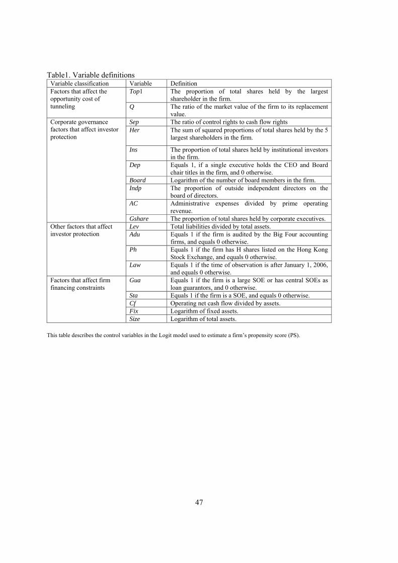
47  

Table1. Variable definitions Variable classification Variable Definition Factors that affect the opportunity cost of tunneling

Top1 The proportion of total shares held by the largest shareholder in the firm.

Q The ratio of the market value of the firm to its replacement value.

Corporate governance factors that affect investor protection

Sep The ratio of control rights to cash flow rights Her The sum of squared proportions of total shares held by the 5

largest shareholders in the firm.

Ins The proportion of total shares held by institutional investors in the firm.

Dep Equals 1, if a single executive holds the CEO and Board chair titles in the firm, and 0 otherwise.

Board Logarithm of the number of board members in the firm. Indp The proportion of outside independent directors on the

board of directors. AC Administrative expenses divided by prime operating

revenue. Gshare The proportion of total shares held by corporate executives.

Other factors that affect investor protection

Lev Total liabilities divided by total assets. Adu Equals 1 if the firm is audited by the Big Four accounting

firms, and equals 0 otherwise. Ph Equals 1 if the firm has H shares listed on the Hong Kong

Stock Exchange, and equals 0 otherwise. Law Equals 1 if the time of observation is after January 1, 2006,

and equals 0 otherwise. Factors that affect firm financing constraints

Gua Equals 1 if the firm is a large SOE or has central SOEs as loan guarantors, and 0 otherwise.

Sta Equals 1 if the firm is a SOE, and equals 0 otherwise. Cf Operating net cash flow divided by assets. Fix Logarithm of fixed assets. Size Logarithm of total assets.

This table describes the control variables in the Logit model used to estimate a firm’s propensity score (PS).

   

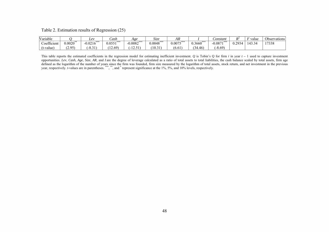
48  

Table 2. Estimation results of Regression (25) 

Variable Q Lev Cash Age Size AR I Constant R2 F value ObservationsCoefficient (t-value)

0.0020** (2.95)

-0.0216*** (-8.31)

0.0551*** (12.69)

-0.0082*** (-12.51)

0.0048*** (10.31)

0.0075*** (6.61)

0.3660*** (34.46)

-0.0871*** (-8.69)

0.2934 143.34 17338

 This table reports the estimated coefficients in the regression model for estimating inefficient investment. Q is Tobin’s Q for firm i in year t – 1 used to capture investment opportunities. Lev, Cash, Age, Size, AR, and I are the degree of leverage calculated as a ratio of total assets to total liabilities, the cash balance scaled by total assets, firm age defined as the logarithm of the number of years since the firm was founded, firm size measured by the logarithm of total assets, stock return, and net investment in the previous year, respectively. t-values are in parentheses. ***, **, and * represent significance at the 1%, 5%, and 10% levels, respectively.

 

   

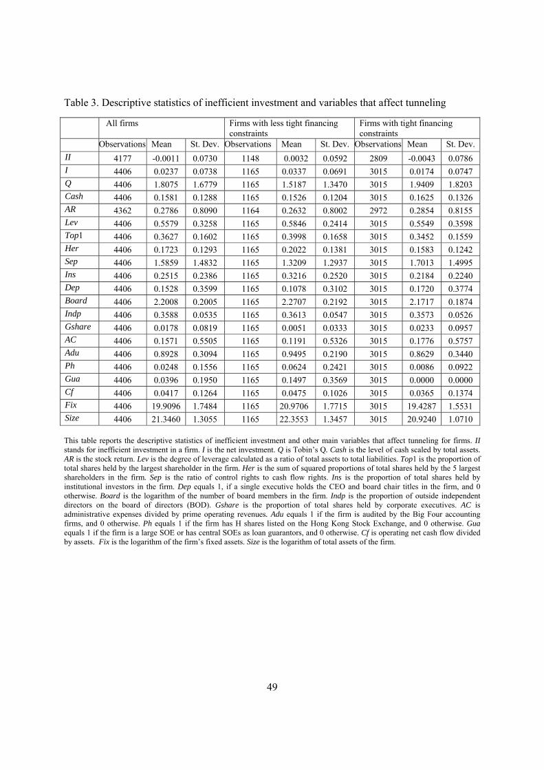
49  

Table 3. Descriptive statistics of inefficient investment and variables that affect tunneling

All firms Firms with less tight financing constraints

Firms with tight financing constraints

Observations Mean St. Dev. Observations Mean St. Dev. Observations Mean St. Dev.

II 4177 -0.0011 0.0730 1148 0.0032 0.0592 2809 -0.0043 0.0786 I 4406 0.0237 0.0738 1165 0.0337 0.0691 3015 0.0174 0.0747 Q 4406 1.8075 1.6779 1165 1.5187 1.3470 3015 1.9409 1.8203 Cash 4406 0.1581 0.1288 1165 0.1526 0.1204 3015 0.1625 0.1326 AR 4362 0.2786 0.8090 1164 0.2632 0.8002 2972 0.2854 0.8155 Lev 4406 0.5579 0.3258 1165 0.5846 0.2414 3015 0.5549 0.3598 Top1 4406 0.3627 0.1602 1165 0.3998 0.1658 3015 0.3452 0.1559 Her 4406 0.1723 0.1293 1165 0.2022 0.1381 3015 0.1583 0.1242 Sep 4406 1.5859 1.4832 1165 1.3209 1.2937 3015 1.7013 1.4995 Ins 4406 0.2515 0.2386 1165 0.3216 0.2520 3015 0.2184 0.2240 Dep 4406 0.1528 0.3599 1165 0.1078 0.3102 3015 0.1720 0.3774 Board 4406 2.2008 0.2005 1165 2.2707 0.2192 3015 2.1717 0.1874 Indp 4406 0.3588 0.0535 1165 0.3613 0.0547 3015 0.3573 0.0526 Gshare 4406 0.0178 0.0819 1165 0.0051 0.0333 3015 0.0233 0.0957 AC 4406 0.1571 0.5505 1165 0.1191 0.5326 3015 0.1776 0.5757 Adu 4406 0.8928 0.3094 1165 0.9495 0.2190 3015 0.8629 0.3440 Ph 4406 0.0248 0.1556 1165 0.0624 0.2421 3015 0.0086 0.0922 Gua 4406 0.0396 0.1950 1165 0.1497 0.3569 3015 0.0000 0.0000 Cf 4406 0.0417 0.1264 1165 0.0475 0.1026 3015 0.0365 0.1374 Fix 4406 19.9096 1.7484 1165 20.9706 1.7715 3015 19.4287 1.5531 Size 4406 21.3460 1.3055 1165 22.3553 1.3457 3015 20.9240 1.0710 This table reports the descriptive statistics of inefficient investment and other main variables that affect tunneling for firms. II stands for inefficient investment in a firm. I is the net investment. Q is Tobin’s Q. Cash is the level of cash scaled by total assets. AR is the stock return. Lev is the degree of leverage calculated as a ratio of total assets to total liabilities. Top1 is the proportion of total shares held by the largest shareholder in the firm. Her is the sum of squared proportions of total shares held by the 5 largest shareholders in the firm. Sep is the ratio of control rights to cash flow rights. Ins is the proportion of total shares held by institutional investors in the firm. Dep equals 1, if a single executive holds the CEO and board chair titles in the firm, and 0 otherwise. Board is the logarithm of the number of board members in the firm. Indp is the proportion of outside independent directors on the board of directors (BOD). Gshare is the proportion of total shares held by corporate executives. AC is administrative expenses divided by prime operating revenues. Adu equals 1 if the firm is audited by the Big Four accounting firms, and 0 otherwise. Ph equals 1 if the firm has H shares listed on the Hong Kong Stock Exchange, and 0 otherwise. Gua equals 1 if the firm is a large SOE or has central SOEs as loan guarantors, and 0 otherwise. Cf is operating net cash flow divided by assets. Fix is the logarithm of the firm’s fixed assets. Size is the logarithm of total assets of the firm.

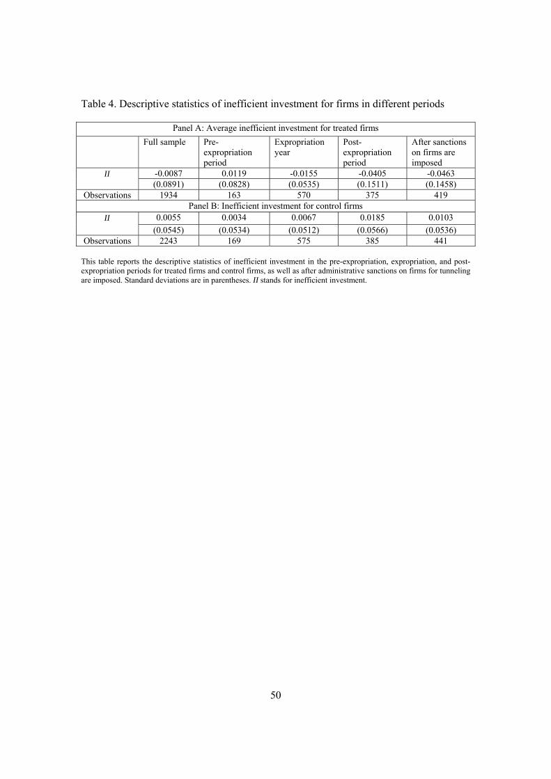
50  

Table 4. Descriptive statistics of inefficient investment for firms in different periods

Panel A: Average inefficient investment for treated firms

Full sample Pre-expropriation period

Expropriation year

Post-expropriation period

After sanctions on firms are imposed

II -0.0087 0.0119 -0.0155 -0.0405 -0.0463 (0.0891) (0.0828) (0.0535) (0.1511) (0.1458)

Observations 1934 163 570 375 419 Panel B: Inefficient investment for control firms

II 0.0055 0.0034 0.0067 0.0185 0.0103

(0.0545) (0.0534) (0.0512) (0.0566) (0.0536) Observations 2243 169 575 385 441

This table reports the descriptive statistics of inefficient investment in the pre-expropriation, expropriation, and post-expropriation periods for treated firms and control firms, as well as after administrative sanctions on firms for tunneling are imposed. Standard deviations are in parentheses. II stands for inefficient investment.

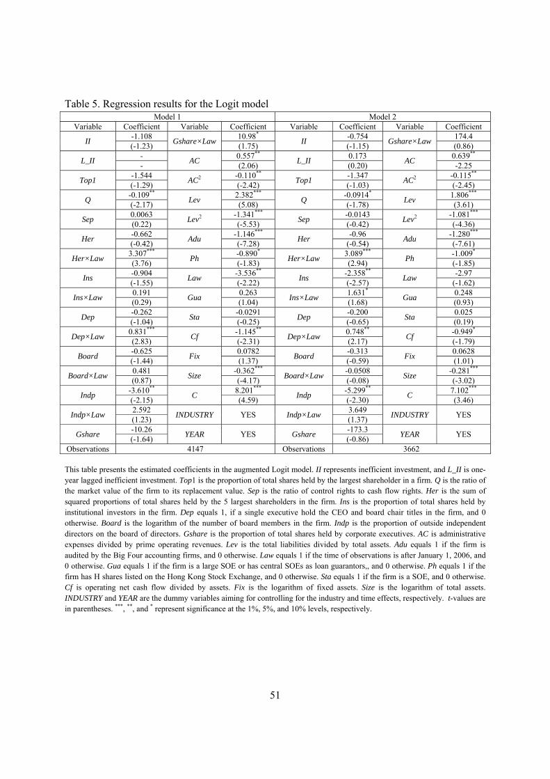
51  

Table 5. Regression results for the Logit model Model 1 Model 2

Variable Coefficient Variable Coefficient Variable Coefficient Variable Coefficient

II -1.108

Gshare×Law 10.98*

II -0.754

Gshare×Law 174.4

(-1.23) (1.75) (-1.15) (0.86)

L_II -

AC 0.557**

L_II 0.173

AC 0.639**

- (2.06) (0.20) -2.25

Top1 -1.544

AC2 -0.110**

Top1 -1.347

AC2 -0.115**

(-1.29) (-2.42) (-1.03) (-2.45)

Q -0.109**

Lev 2.382***

Q -0.0914*

Lev 1.806***

(-2.17) (5.08) (-1.78) (3.61)

Sep 0.0063

Lev2 -1.341***

Sep -0.0143

Lev2 -1.081***

(0.22) (-5.53) (-0.42) (-4.36)

Her -0.662

Adu -1.146***

Her -0.96

Adu -1.280***

(-0.42) (-7.28) (-0.54) (-7.61)

Her×Law 3.307***

Ph -0.890*

Her×Law 3.089***

Ph -1.009*

(3.76) (-1.83) (2.94) (-1.85)

Ins -0.904

Law -3.536**

Ins -2.358**

Law -2.97

(-1.55) (-2.22) (-2.57) (-1.62)

Ins×Law 0.191

Gua 0.263

Ins×Law 1.631*

Gua 0.248

(0.29) (1.04) (1.68) (0.93)

Dep -0.262

Sta -0.0291

Dep -0.200

Sta 0.025

(-1.04) (-0.25) (-0.65) (0.19)

Dep×Law 0.831***

Cf -1.145**

Dep×Law 0.748**

Cf -0.949*

(2.83) (-2.31) (2.17) (-1.79)

Board -0.625

Fix 0.0782

Board -0.313

Fix 0.0628

(-1.44) (1.37) (-0.59) (1.01)

Board×Law 0.481

Size -0.362***

Board×Law -0.0508

Size -0.281***

(0.87) (-4.17) (-0.08) (-3.02)

Indp -3.610**

C 8.201***

Indp -5.299**

C 7.102***

(-2.15) (4.59) (-2.30) (3.46)

Indp×Law 2.592 

INDUSTRY YES Indp×Law 3.649

INDUSTRY YES (1.23)  (1.37)

Gshare -10.26 

YEAR YES Gshare -173.3

YEAR YES (-1.64)  (-0.86)

Observations 4147 Observations 3662 This table presents the estimated coefficients in the augmented Logit model. II represents inefficient investment, and L_II is one-year lagged inefficient investment. Top1 is the proportion of total shares held by the largest shareholder in a firm. Q is the ratio of the market value of the firm to its replacement value. Sep is the ratio of control rights to cash flow rights. Her is the sum of squared proportions of total shares held by the 5 largest shareholders in the firm. Ins is the proportion of total shares held by institutional investors in the firm. Dep equals 1, if a single executive hold the CEO and board chair titles in the firm, and 0 otherwise. Board is the logarithm of the number of board members in the firm. Indp is the proportion of outside independent directors on the board of directors. Gshare is the proportion of total shares held by corporate executives. AC is administrative expenses divided by prime operating revenues. Lev is the total liabilities divided by total assets. Adu equals 1 if the firm is audited by the Big Four accounting firms, and 0 otherwise. Law equals 1 if the time of observations is after January 1, 2006, and 0 otherwise. Gua equals 1 if the firm is a large SOE or has central SOEs as loan guarantors,, and 0 otherwise. Ph equals 1 if the firm has H shares listed on the Hong Kong Stock Exchange, and 0 otherwise. Sta equals 1 if the firm is a SOE, and 0 otherwise. Cf is operating net cash flow divided by assets. Fix is the logarithm of fixed assets. Size is the logarithm of total assets. INDUSTRY and YEAR are the dummy variables aiming for controlling for the industry and time effects, respectively. t-values are in parentheses. ***, **, and * represent significance at the 1%, 5%, and 10% levels, respectively.

   

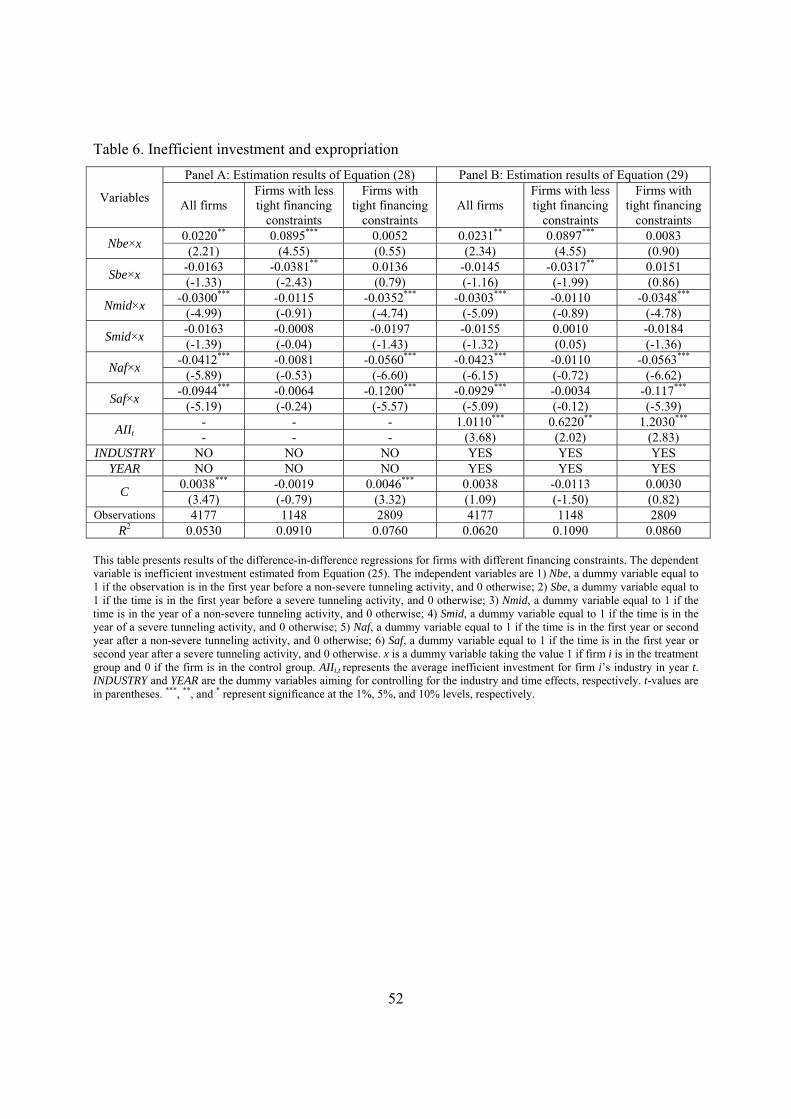
52  

Table 6. Inefficient investment and expropriation   

Variables

Panel A: Estimation results of Equation (28) Panel B: Estimation results of Equation (29)

All firms Firms with less tight financing

constraints

Firms with tight financing

constraints All firms

Firms with less tight financing

constraints

Firms with tight financing

constraints

Nbe×x 0.0220** 0.0895*** 0.0052 0.0231** 0.0897*** 0.0083 (2.21) (4.55) (0.55) (2.34) (4.55) (0.90)

Sbe×x -0.0163 -0.0381** 0.0136 -0.0145 -0.0317** 0.0151 (-1.33) (-2.43) (0.79) (-1.16) (-1.99) (0.86)

Nmid×x -0.0300*** -0.0115 -0.0352*** -0.0303*** -0.0110 -0.0348***

(-4.99) (-0.91) (-4.74) (-5.09) (-0.89) (-4.78)

Smid×x -0.0163 -0.0008 -0.0197 -0.0155 0.0010 -0.0184 (-1.39) (-0.04) (-1.43) (-1.32) (0.05) (-1.36)

Naf×x -0.0412*** -0.0081 -0.0560*** -0.0423*** -0.0110 -0.0563***

(-5.89) (-0.53) (-6.60) (-6.15) (-0.72) (-6.62)

Saf×x -0.0944*** -0.0064 -0.1200*** -0.0929*** -0.0034 -0.117***

(-5.19) (-0.24) (-5.57) (-5.09) (-0.12) (-5.39)

AIIt - - - 1.0110*** 0.6220** 1.2030*** - - - (3.68) (2.02) (2.83)

INDUSTRY NO NO NO YES YES YES YEAR NO NO NO YES YES YES

C 0.0038*** -0.0019 0.0046*** 0.0038 -0.0113 0.0030

(3.47) (-0.79) (3.32) (1.09) (-1.50) (0.82) Observations 4177 1148 2809 4177 1148 2809

R2 0.0530 0.0910 0.0760 0.0620 0.1090 0.0860 This table presents results of the difference-in-difference regressions for firms with different financing constraints. The dependent variable is inefficient investment estimated from Equation (25). The independent variables are 1) Nbe, a dummy variable equal to 1 if the observation is in the first year before a non-severe tunneling activity, and 0 otherwise; 2) Sbe, a dummy variable equal to 1 if the time is in the first year before a severe tunneling activity, and 0 otherwise; 3) Nmid, a dummy variable equal to 1 if the time is in the year of a non-severe tunneling activity, and 0 otherwise; 4) Smid, a dummy variable equal to 1 if the time is in the year of a severe tunneling activity, and 0 otherwise; 5) Naf, a dummy variable equal to 1 if the time is in the first year or second year after a non-severe tunneling activity, and 0 otherwise; 6) Saf, a dummy variable equal to 1 if the time is in the first year or second year after a severe tunneling activity, and 0 otherwise. x is a dummy variable taking the value 1 if firm i is in the treatment group and 0 if the firm is in the control group. AIIi,t represents the average inefficient investment for firm i’s industry in year t. INDUSTRY and YEAR are the dummy variables aiming for controlling for the industry and time effects, respectively. t-values are in parentheses. ***, **, and * represent significance at the 1%, 5%, and 10% levels, respectively.

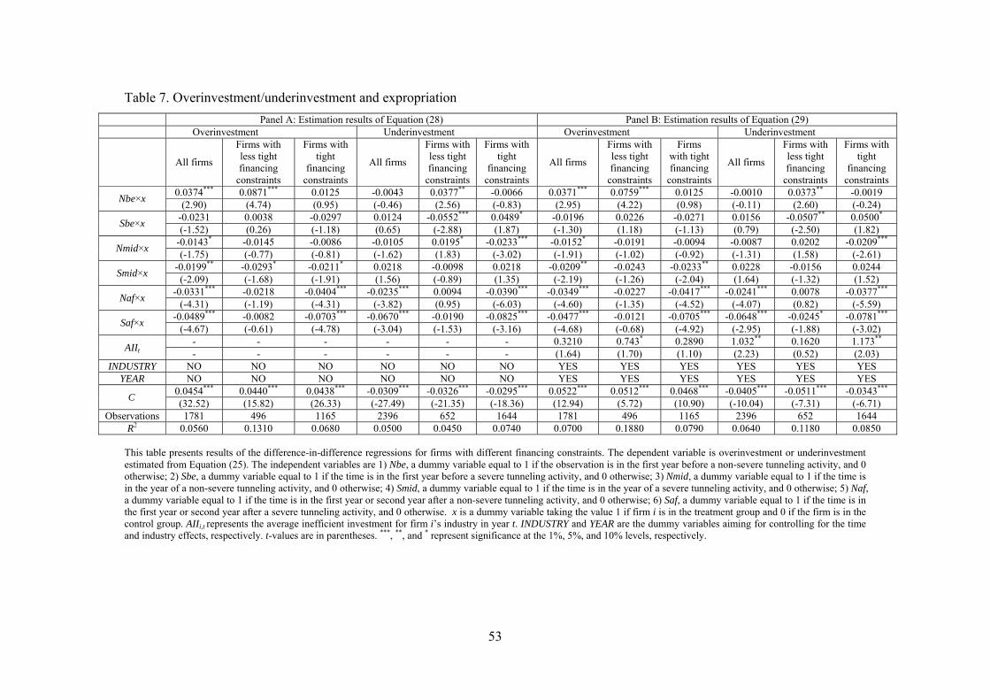
53  

Table 7. Overinvestment/underinvestment and expropriation

Panel A: Estimation results of Equation (28) Panel B: Estimation results of Equation (29) Overinvestment Underinvestment Overinvestment Underinvestment

All firms

Firms with less tight financing

constraints

Firms with tight

financing constraints

All firms

Firms with less tight financing

constraints

Firms with tight

financing constraints

All firms

Firms with less tight financing

constraints

Firms with tight financing

constraints

All firms

Firms with less tight financing

constraints

Firms with tight

financing constraints

Nbe×x 0.0374*** 0.0871*** 0.0125 -0.0043 0.0377** -0.0066 0.0371*** 0.0759*** 0.0125 -0.0010 0.0373** -0.0019

(2.90) (4.74) (0.95) (-0.46) (2.56) (-0.83) (2.95) (4.22) (0.98) (-0.11) (2.60) (-0.24)

Sbe×x -0.0231 0.0038 -0.0297 0.0124 -0.0552*** 0.0489* -0.0196 0.0226 -0.0271 0.0156 -0.0507** 0.0500* (-1.52) (0.26) (-1.18) (0.65) (-2.88) (1.87) (-1.30) (1.18) (-1.13) (0.79) (-2.50) (1.82)

Nmid×x -0.0143* -0.0145 -0.0086 -0.0105 0.0195* -0.0233*** -0.0152* -0.0191 -0.0094 -0.0087 0.0202 -0.0209*** (-1.75) (-0.77) (-0.81) (-1.62) (1.83) (-3.02) (-1.91) (-1.02) (-0.92) (-1.31) (1.58) (-2.61)

Smid×x -0.0199** -0.0293* -0.0211* 0.0218 -0.0098 0.0218 -0.0209** -0.0243 -0.0233** 0.0228 -0.0156 0.0244

(-2.09) (-1.68) (-1.91) (1.56) (-0.89) (1.35) (-2.19) (-1.26) (-2.04) (1.64) (-1.32) (1.52)

Naf×x -0.0331*** -0.0218 -0.0404*** -0.0235*** 0.0094 -0.0390*** -0.0349*** -0.0227 -0.0417*** -0.0241*** 0.0078 -0.0377***

(-4.31) (-1.19) (-4.31) (-3.82) (0.95) (-6.03) (-4.60) (-1.35) (-4.52) (-4.07) (0.82) (-5.59)

Saf×x -0.0489*** -0.0082 -0.0703*** -0.0670*** -0.0190 -0.0825*** -0.0477*** -0.0121 -0.0705*** -0.0648*** -0.0245* -0.0781***

(-4.67) (-0.61) (-4.78) (-3.04) (-1.53) (-3.16) (-4.68) (-0.68) (-4.92) (-2.95) (-1.88) (-3.02)

AIIt - - - - - - 0.3210 0.743* 0.2890 1.032** 0.1620 1.173** - - - - - - (1.64) (1.70) (1.10) (2.23) (0.52) (2.03)

INDUSTRY NO NO NO NO NO NO YES YES YES YES YES YES YEAR NO NO NO NO NO NO YES YES YES YES YES YES

C 0.0454*** 0.0440*** 0.0438*** -0.0309*** -0.0326*** -0.0295*** 0.0522*** 0.0512*** 0.0468*** -0.0405*** -0.0511*** -0.0343*** (32.52) (15.82) (26.33) (-27.49) (-21.35) (-18.36) (12.94) (5.72) (10.90) (-10.04) (-7.31) (-6.71)

Observations 1781 496 1165 2396 652 1644 1781 496 1165 2396 652 1644 R2 0.0560 0.1310 0.0680 0.0500 0.0450 0.0740 0.0700 0.1880 0.0790 0.0640 0.1180 0.0850

This table presents results of the difference-in-difference regressions for firms with different financing constraints. The dependent variable is overinvestment or underinvestment estimated from Equation (25). The independent variables are 1) Nbe, a dummy variable equal to 1 if the observation is in the first year before a non-severe tunneling activity, and 0 otherwise; 2) Sbe, a dummy variable equal to 1 if the time is in the first year before a severe tunneling activity, and 0 otherwise; 3) Nmid, a dummy variable equal to 1 if the time is in the year of a non-severe tunneling activity, and 0 otherwise; 4) Smid, a dummy variable equal to 1 if the time is in the year of a severe tunneling activity, and 0 otherwise; 5) Naf, a dummy variable equal to 1 if the time is in the first year or second year after a non-severe tunneling activity, and 0 otherwise; 6) Saf, a dummy variable equal to 1 if the time is in the first year or second year after a severe tunneling activity, and 0 otherwise. x is a dummy variable taking the value 1 if firm i is in the treatment group and 0 if the firm is in the control group. AIIi,t represents the average inefficient investment for firm i’s industry in year t. INDUSTRY and YEAR are the dummy variables aiming for controlling for the time and industry effects, respectively. t-values are in parentheses. ***, **, and * represent significance at the 1%, 5%, and 10% levels, respectively.

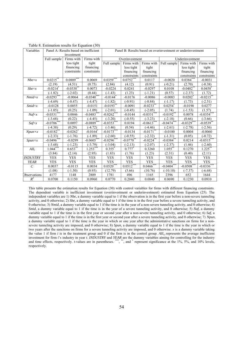
54  

Table 8. Estimation results for Equation (30) Variables Panel A: Results based on inefficient

investment Panel B: Results based on overinvestment or underinvestment

Full sample Firms with less tight financing

constraints

Firms with tight

financing constraints

Overinvestment Underinvestment Full sample Firms with

less tight financing

constraints

Firms with tight

financing constraints

Full sample Firms with less tight financing

constraints

Firms with tight

financing constraints

Nbe×x 0.0215** 0.0889*** 0.0069 0.0359*** 0.0752*** 0.0117 -0.0020 0.0384*** -0.0031 (2.19) (4.51) (0.75) (2.84) (4.12) (0.91) (-0.21) (2.70) (-0.38)

Sbe×x -0.0214* -0.0338** 0.0073 -0.0224 0.0241 -0.0297 0.0108 -0.0482** 0.0458* (-1.82) (-2.02) (0.44) (-1.43) (1.23) (-1.21) (0.57) (-2.37) (1.72)

Nmid×x -0.0293*** -0.0064 -0.0340*** -0.0144* -0.0176 -0.0086 -0.0083 0.0202* -0.0215** (-4.69) (-0.47) (-4.47) (-1.82) (-0.91) (-0.84) (-1.17) (1.73) (-2.51)

Smid×x -0.0128 0.0055 -0.0151 -0.0193** -0.0091 -0.0233** 0.0254* -0.0190 0.0277 (-1.05) (0.25) (-1.09) (-2.01) (-0.45) (-2.05) (1.74) (-1.53) (1.57)

Naf×x -0.0331*** 0.0046 -0.0483*** -0.0262*** -0.0144 -0.0331*** -0.0192** 0.0078 -0.0354*** (-3.68) (0.22) (-4.45) (-3.20) (-0.55) (-3.23) (-2.18) (0.66) (-3.66)

Saf×x -0.0706*** 0.0097 -0.0889*** -0.0353*** 0.0194 -0.0613*** -0.0474*** -0.0329*** -0.0539** (-4.38) (0.29) (-4.72) (-3.46) (0.54) (-4.46) (-2.61) (-2.78) (-2.56)

Npun×x -0.0182** -0.0262* -0.0164* -0.0173*** -0.0134 -0.0171** -0.0100 0.0004 -0.0060 (-2.33) (-1.76) (-1.89) (-2.60) (-0.55) (-2.32) (-1.31) (0.05) (-0.72)

Spun×x -0.0496*** -0.0299 -0.0605*** -0.0296*** -0.0770** -0.0224** -0.0384** 0.0214 -0.0515*** (-3.68) (-1.23) (-3.79) (-3.04) (-2.13) (-2.07) (-2.37) (1.46) (-2.60)

AIIt 1.044*** 0.653** 1.253*** 0.355* 0.777* 0.3260 1.055** 0.1270 1.225** (3.84) (2.14) (2.95) (1.83) (1.76) (1.23) (2.31) (0.40) (2.11)

INDUSTRY YES YES YES YES YES YES YES YES YES YEAR YES YES YES YES YES YES YES YES YES

C 0.0037 -0.0115 0.0034 0.0520*** 0.0512*** 0.0466*** -0.0404*** -0.0508*** -0.0336*** (1.08) (-1.50) (0.93) (12.79) (5.66) (10.76) (-10.10) (-7.37) (-6.68)

Observations 4177 1148 2809 1781 496 1165 2396 652 1644 R2 0.0700 0.1150 0.0960 0.0770 0.2040 0.0840 0.0690 0.1230 0.0910

This table presents the estimation results for Equation (30) with control variables for firms with different financing constraints. The dependent variable is inefficient investment (overinvestment or underinvestment) estimated from Equation (25). The independent variables are 1) Nbe, a dummy variable equal to 1 if the observation is in the first year before a non-severe tunneling activity, and 0 otherwise; 2) Sbe, a dummy variable equal to 1 if the time is in the first year before a severe tunneling activity, and 0 otherwise; 3) Nmid, a dummy variable equal to 1 if the time is in the year of a non-severe tunneling activity, and 0 otherwise; 4) Smid, a dummy variable equal to 1 if the time is in the year of a severe tunneling activity, and 0 otherwise; 5) Naf, a dummy variable equal to 1 if the time is in the first year or second year after a non-severe tunneling activity, and 0 otherwise; 6) Saf, a dummy variable equal to 1 if the time is in the first year or second year after a severe tunneling activity, and 0 otherwise; 7) Npun, a dummy variable equal to 1 if the time is the year in which or one year after the administrative sanctions on firms for a non-severe tunneling activity are imposed, and 0 otherwise; 8) Spun, a dummy variable equal to 1 if the time is the year in which or two years after the sanctions on firms for a severe tunneling activity are imposed, and 0 otherwise. x is a dummy variable taking the value 1 if firm i is in the treatment group and 0 if the firm is in the control group. AIIi,t represents the average inefficient investment for firm i’s industry in year t. INDUSTRY and YEAR are the dummy variables aiming for controlling for the industry and time effects, respectively. t-values are in parentheses. ***, **, and * represent significance at the 1%, 5%, and 10% levels, respectively.

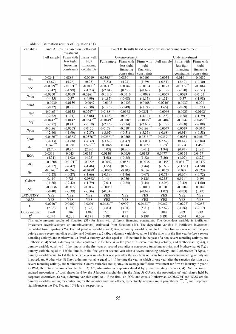
55  

Table 9. Estimation results of Equation (31) Variables Panel A: Results based on inefficient

investment Panel B: Results based on overinvestment or underinvestment

Full sample Firms with less tight financing

constraints

Firms with tight

financing constraints

Overinvestment Underinvestment Full sample Firms with

less tight financing

constraints

Firms with tight

financing constraints

Full sample Firms with less tight financing

constraints

Firms with tight

financing constraints

Nbe 0.0241*** 0.0886*** 0.0019 0.0365*** 0.0830*** 0.0101 -0.0054 0.0191** -0.0032

(2.69) (4.76) (0.25) (3.23) (4.24) (1.29) (-0.51) (2.42) (-0.30)

Sbe -0.0309*** -0.0171** -0.0181* -0.0211** 0.0046 -0.0104 -0.0173 -0.0372** -0.0064

(-3.42) (-1.99) (-1.73) (-2.04) (0.59) (-0.67) (-1.39) (-2.50) (-0.51)

Nmid -0.0200*** 0.0059 -0.0261*** -0.0110* -0.0016 -0.0088 -0.0067 0.0029 -0.0123**

(-4.35) -0.57 (-4.99) (-1.87) (-0.08) (-1.13) (-1.31) -0.37 (-1.98)

Smid -0.0030 0.0159 -0.0047 -0.0108 -0.0123 -0.0168* 0.0216* -0.0037 0.021 (-0.22) (0.75) (-0.30) (-1.25) (-0.49) (-1.74) (1.65) (-0.69) （1.52）

Naf -0.0165** 0.0152 -0.0247*** -0.0188*** 0.0162 -0.0251*** -0.0066 -0.0023 -0.0102*

(-2.22) (1.01) (-3.06) (-3.13) (0.90) (-4.10) (-1.53) (-0.28) (-1.79)

Saf -0.0447*** 0.0142 -0.0547*** -0.0149** -0.0089 -0.0175** -0.0404* -0.0042 -0.0486**

(-2.87) (0.41) (-3.19) (-2.16) (-0.14) (-2.60) (-1.78) (-0.68) (-2.08)

Npun -0.0168** -0.0268* -0.0150** -0.0179*** -0.0104 -0.0168*** -0.0047 0.0039 -0.0046

(-2.60) (-1.90) (-2.37) (-3.92) (-0.51) (-3.35) (-0.68) (0.91) (-0.58)

Spun -0.0486*** -0.0383* -0.0576*** -0.0256*** -0.0668 -0.0215*** -0.0359*** 0.0034 -0.0461***

(-4.13) (-1.68) (-4.32) (-3.62) (-1.47) (-3.03) (-2.87) (0.44) (-3.04)

AII 1.142*** 0.350 1.522*** 0.0066 0.144 0.0022 1.369* 0.394 1.457* (2.70) (0.96) (2.76) (0.03) (0.30) (0.01) (1.94) (0.93) (1.85)

ROA 0.0319*** -0.0434 0.0335*** 0.0130* -0.0059 0.0143* 0.0477*** 0.0354 0.0477***

(4.31) (-1.02) (4.73) (1.68) (-0.35) (1.82) (3.26) (1.02) (3.22)

AC -0.0208 -0.0171** -0.0225 0.0042 0.0551 0.0036 -0.0455* -0.0331*** -0.0477 (-1.52) (-2.42) (-1.46) (1.55) (0.62) (1.44) (-1.68) (-11.51) (-1.50)

Her -0.0543** -0.0243 -0.0478* -0.0039 -0.203 0.014 -0.0169 0.027 -0.0234

(-2.28) (-0.27) (-1.66) (-0.19) (-1.46) (0.67) (-0.71) (0.66) (-0.72)

Gshare -0.110* -0.721** -0.0862* 0.146** -0.0564 0.125 -0.255** -0.991*** -0.191 (-1.86) (-2.42) (-1.79) (2.01) (-0.24) (1.44) (-2.06) (-3.42) (-1.60)

Sta -0.0036 -0.0072 -0.0037 -0.0035 -0.0037 0.0103 -0.0002 0.016 (-0.40) (-0.39) (-0.36) (-0.34) (-0.67) (1.02) (-0.03) (1.43)

INDUSTRY YES YES YES YES YES YES YES YES YES YEAR YES YES YES YES YES YES YES YES YES

C 0.0220** 0.0402* 0.0201* 0.0423*** 0.0992*** 0.0423*** -0.0262*** -0.0227* -0.0253**

(2.33) (1.93) (1.76) (4.83) (3.01) (5.81) (-2.67) (-1.86) (-2.17) Observations 1768 386 1382 720 177 543 1048 209 839

R2 0.145 0.301 0.171 0.182 0.42 0.198 0.191 0.544 0.206 This table presents results of Equation (31) for firms with different financing constraints. The dependent variable is inefficient investment (overinvestment or underinvestment) estimated from Equation (25). The dependent variable is inefficient investment calculated from Equation (25). The independent variables are 1) Nbe, a dummy variable equal to 1 if the observation is in the first year before a non-severe tunneling activity, and 0 otherwise; 2) Sbe, a dummy variable equal to 1 if the time is in the first year before a severe tunneling activity, and 0 otherwise; 3) Nmid, a dummy variable equal to 1 if the time is in the year of a non-severe tunneling activity, and 0 otherwise; 4) Smid, a dummy variable equal to 1 if the time is in the year of a severe tunneling activity, and 0 otherwise; 5) Naf, a dummy variable equal to 1 if the time is in the first year or second year after a non-severe tunneling activity, and 0 otherwise; 6) Saf, a dummy variable equal to 1 if the time is in the first year or second year after a severe tunneling activity, and 0 otherwise; 7) Npun, a dummy variable equal to 1 if the time is the year in which or one year after the sanctions on firms for a non-severe tunneling activity are imposed, and 0 otherwise; 8) Spun, a dummy variable equal to 1 if the time the year in which or one year after the sanction decision on a severe tunneling activity, and 0 otherwise. Control variables are: 1) AIIi,t, the average inefficient investment for firm i’s industry in year t; 2) ROA, the return on assets for the firm; 3) AC, administrative expenses divided by prime operating revenues; 4) Her, the sum of squared proportions of total shares held by the 5 largest shareholders in the firm; 5) Gshare, the proportion of total shares held by corporate executives. 6) Sta, a dummy variable equal to 1 if the firm is a SOE, and equals 0 otherwise. INDUSTRY and YEAR are the dummy variables aiming for controlling for the industry and time effects, respectively. t-values are in parentheses. ***, **, and * represent significance at the 1%, 5%, and 10% levels, respectively.

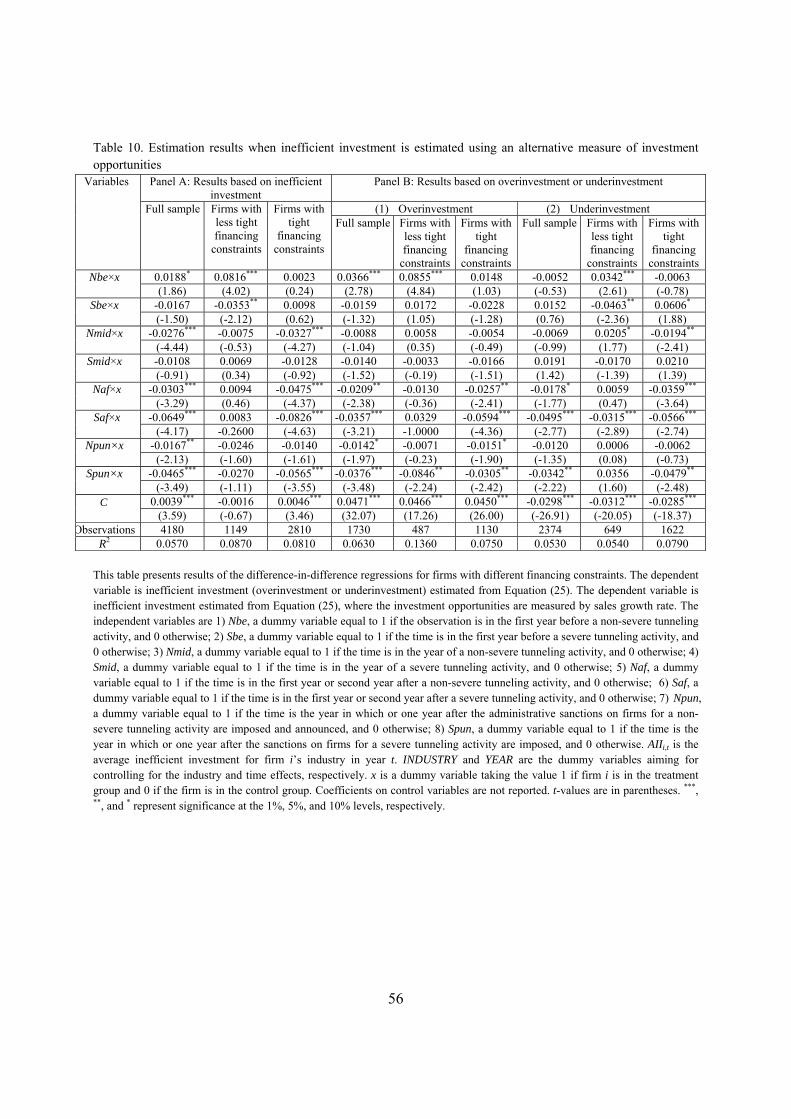
56  

Table 10. Estimation results when inefficient investment is estimated using an alternative measure of investment opportunities

Variables Panel A: Results based on inefficient investment

Panel B: Results based on overinvestment or underinvestment

Full sample Firms with less tight financing

constraints

Firms with tight

financing constraints

(1) Overinvestment (2) Underinvestment Full sample Firms with

less tight financing

constraints

Firms with tight

financing constraints

Full sample Firms with less tight financing

constraints

Firms with tight

financing constraints

Nbe×x 0.0188* 0.0816*** 0.0023 0.0366*** 0.0855*** 0.0148 -0.0052 0.0342*** -0.0063 (1.86) (4.02) (0.24) (2.78) (4.84) (1.03) (-0.53) (2.61) (-0.78)

Sbe×x -0.0167 -0.0353** 0.0098 -0.0159 0.0172 -0.0228 0.0152 -0.0463** 0.0606* (-1.50) (-2.12) (0.62) (-1.32) (1.05) (-1.28) (0.76) (-2.36) (1.88)

Nmid×x -0.0276*** -0.0075 -0.0327*** -0.0088 0.0058 -0.0054 -0.0069 0.0205* -0.0194** (-4.44) (-0.53) (-4.27) (-1.04) (0.35) (-0.49) (-0.99) (1.77) (-2.41)

Smid×x -0.0108 0.0069 -0.0128 -0.0140 -0.0033 -0.0166 0.0191 -0.0170 0.0210 (-0.91) (0.34) (-0.92) (-1.52) (-0.19) (-1.51) (1.42) (-1.39) (1.39)

Naf×x -0.0303*** 0.0094 -0.0475*** -0.0209** -0.0130 -0.0257** -0.0178* 0.0059 -0.0359*** (-3.29) (0.46) (-4.37) (-2.38) (-0.36) (-2.41) (-1.77) (0.47) (-3.64)

Saf×x -0.0649*** 0.0083 -0.0826*** -0.0357*** 0.0329 -0.0594*** -0.0495*** -0.0315*** -0.0566*** (-4.17) -0.2600 (-4.63) (-3.21) -1.0000 (-4.36) (-2.77) (-2.89) (-2.74)

Npun×x -0.0167** -0.0246 -0.0140 -0.0142* -0.0071 -0.0151* -0.0120 0.0006 -0.0062 (-2.13) (-1.60) (-1.61) (-1.97) (-0.23) (-1.90) (-1.35) (0.08) (-0.73)

Spun×x -0.0465*** -0.0270 -0.0565*** -0.0376*** -0.0846** -0.0305** -0.0342** 0.0356 -0.0479** (-3.49) (-1.11) (-3.55) (-3.48) (-2.24) (-2.42) (-2.22) (1.60) (-2.48)

C 0.0039*** -0.0016 0.0046*** 0.0471*** 0.0466*** 0.0450*** -0.0298*** -0.0312*** -0.0285*** (3.59) (-0.67) (3.46) (32.07) (17.26) (26.00) (-26.91) (-20.05) (-18.37)

Observations 4180 1149 2810 1730 487 1130 2374 649 1622 R2 0.0570 0.0870 0.0810 0.0630 0.1360 0.0750 0.0530 0.0540 0.0790

This table presents results of the difference-in-difference regressions for firms with different financing constraints. The dependent variable is inefficient investment (overinvestment or underinvestment) estimated from Equation (25). The dependent variable is inefficient investment estimated from Equation (25), where the investment opportunities are measured by sales growth rate. The independent variables are 1) Nbe, a dummy variable equal to 1 if the observation is in the first year before a non-severe tunneling activity, and 0 otherwise; 2) Sbe, a dummy variable equal to 1 if the time is in the first year before a severe tunneling activity, and 0 otherwise; 3) Nmid, a dummy variable equal to 1 if the time is in the year of a non-severe tunneling activity, and 0 otherwise; 4) Smid, a dummy variable equal to 1 if the time is in the year of a severe tunneling activity, and 0 otherwise; 5) Naf, a dummy variable equal to 1 if the time is in the first year or second year after a non-severe tunneling activity, and 0 otherwise; 6) Saf, a dummy variable equal to 1 if the time is in the first year or second year after a severe tunneling activity, and 0 otherwise; 7) Npun, a dummy variable equal to 1 if the time is the year in which or one year after the administrative sanctions on firms for a non-severe tunneling activity are imposed and announced, and 0 otherwise; 8) Spun, a dummy variable equal to 1 if the time is the year in which or one year after the sanctions on firms for a severe tunneling activity are imposed, and 0 otherwise. AIIi,t is the average inefficient investment for firm i’s industry in year t. INDUSTRY and YEAR are the dummy variables aiming for controlling for the industry and time effects, respectively. x is a dummy variable taking the value 1 if firm i is in the treatment group and 0 if the firm is in the control group. Coefficients on control variables are not reported. t-values are in parentheses. ***, **, and * represent significance at the 1%, 5%, and 10% levels, respectively.

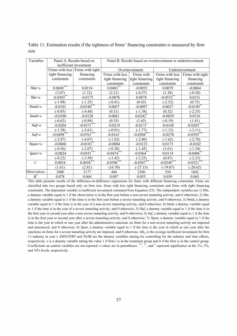
57  

Table 11. Estimation results if the tightness of firms’ financing constraints is measured by firm size

Variables Panel A: Results based on inefficient investment

Panel B: Results based on overinvestment or underinvestment

Firms with less tight financing

constraints

Firms with tight financing

constraints

Overinvestment Underinvestment Firms with less tight financing

constraints

Firms with tight financing

constraints

Firms with less tight financing

constraints

Firms with tight financing

constraints Nbe×x 0.0608*** 0.0154 0.0401** -0.0053 0.0079 -0.0064

(3.07) (1.32) (2.21) (-0.57) (1.38) (-0.58) Sbe×x -0.0303** -0.0175 -0.0076 0.0078 -0.0532** 0.0151

(-1.98) (-1.25) (-0.41) (0.42) (-2.52) (0.73) Nmid×x -0.0101 -0.0340*** 0.0057 -0.0097 0.0027 -0.0190**

(-0.85) (-4.44) (0.31) (-1.38) (0.32) (-2.35) Smid×x -0.0100 -0.0128 0.0061 0.0242* -0.0029 0.0216

(-0.62) (-0.98) (0.35) (1.65) (-0.19) (1.41) Naf×x -0.0204 -0.0371*** -0.0219 -0.0171* -0.0168 -0.0285***

(-1.28) (-3.61) (-0.91) (-1.77) (-1.12) (-3.11) Saf×x -0.0498*** -0.0761*** -0.0161* -0.0504*** -0.0270 -0.0595***

(-2.87) (-4.07) (-1.82) (-2.80) (-1.62) (-2.78) Npun×x -0.0068 -0.0183** -0.0084 -0.0123 0.0173 -0.0102

(-0.56) (-2.07) (-0.38) (-1.45) (1.61) (-1.34) Spun×x -0.0024 -0.0551*** -0.0474*** -0.0364** 0.0114 -0.0406**

(-0.22) (-3.59) (-3.42) (-2.25) (0.87) (-2.23) C 0.0034 0.0038*** 0.0398*** -0.0307*** -0.0249*** -0.0321***

(1.61) (2.81) (16.70) (-27.15) (-19.07) (-20.62) Observations 1000 3177 446 2396 554 1842

R2 0.078 0.064 0.097 0.055 0.039 0.063 This table presents results of the difference-in-difference regressions for firms with different financing constraints. Firms are classified into two groups based only on firm size: firms with less tight financing constraints and firms with tight financing constraints. The dependent variable is inefficient investment estimated from Equation (25). The independent variables are 1) Nbe, a dummy variable equal to 1 if the observation is in the first year before a non-severe tunneling activity, and 0 otherwise; 2) Sbe, a dummy variable equal to 1 if the time is in the first year before a severe tunneling activity, and 0 otherwise; 3) Nmid, a dummy variable equal to 1 if the time is in the year of a non-severe tunneling activity, and 0 otherwise; 4) Smid, a dummy variable equal to 1 if the time is in the year of a severe tunneling activity, and 0 otherwise; 5) Naf, a dummy variable equal to 1 if the time is in the first year or second year after a non-severe tunneling activity, and 0 otherwise; 6) Saf, a dummy variable equal to 1 if the time is in the first year or second year after a severe tunneling activity, and 0 otherwise; 7) Npun, a dummy variable equal to 1 if the time is the year in which or one year after the administrative sanctions on firms for a non-severe tunneling activity are imposed and announced, and 0 otherwise; 8) Spun, a dummy variable equal to 1 if the time is the year in which or one year after the sanctions on firms for a severe tunneling activity are imposed, and 0 otherwise. AIIi,t is the average inefficient investment for firm i’s industry in year t. INDUSTRY and YEAR are the dummy variables aiming for controlling for the industry and time effects, respectively. x is a dummy variable taking the value 1 if firm i is in the treatment group and 0 if the firm is in the control group. Coefficients on control variables are not reported. t-values are in parentheses. ***, **, and * represent significance at the 1%, 5%, and 10% levels, respectively.

58  

Table 12. Estimation results if the treated and control firms are matched using the kernel matching method.

Variables Panel A: Results based on inefficient investment

Panel B: Results based on overinvestment or underinvestment

Full sample Firms with less tight financing

constraints

Firms with tight

financing constraints

Overinvestment Underinvestment Full sample Firms with

less tight financing

constraints

Firms with tight

financing constraints

Full sample Firms with less tight financing

constraints

Firms with tight

financing constraints

Nbe×x 0.0203* 0.0963*** -0.0059 0.0305** 0.0689*** -0.0036 -0.0013 0.0361*** -0.0042 (1.92) (4.51) (-0.55) (2.28) (3.15) (-0.28) (-0.14) (2.96) (-0.53)

Sbe×x -0.0275** -0.0351** -0.0035 -0.0310* -0.0074 -0.0365 0.0055 -0.0402** 0.0284 (-2.34) (-2.04) (-0.23) (-1.89) (-0.71) (-1.41) (0.32) (-2.01) (1.25)

Nmid×x -0.0229*** 0.0017 -0.0303*** -0.0107 -0.0008 -0.0175** -0.0108 0.0026 -0.0178** (-3.33) (0.13) (-3.36) (-1.25) (-0.04) (-1.99) (-1.45) (0.20) (-2.05)

Smid×x -0.0066 0.0107 -0.0099 -0.0143 -0.0073 -0.0111 0.0289* -0.0025 0.0283* (-0.53) (0.51) (-0.68) (-1.39) (-0.46) (-0.93) (1.96) (-0.19) (1.69)

Naf×x -0.0175* 0.0168 -0.0276** -0.0141 -0.0032 -0.0264** -0.0162* 0.0074 -0.0287*** (-1.86) (0.84) (-2.54) (-1.46) (-0.11) (-2.15) (-1.67) (0.57) (-2.98)

Saf×x -0.0443*** 0.0107 -0.0527*** -0.0256** 0.0077 -0.0316** -0.0294** -0.0082 -0.0368** (-2.75) (0.33) (-2.84) (-2.34) (0.23) (-2.41) (-2.01) (-0.75) (-2.16)

Npun×x -0.0201** -0.0254 -0.0210** -0.0116 -0.0032 -0.0092 -0.0131 0.0014 -0.0124 (-2.41) (-1.53) (-2.39) (-1.50) (-0.13) (-1.01) (-1.52) (0.20) (-1.43)

Spun×x -0.0585*** -0.0363 -0.0706*** -0.0200** -0.0465 -0.0213** -0.0484*** 0.0088 -0.0602*** (-4.51) (-1.63) (-4.62) (-2.44) (-1.35) (-2.20) (-3.08) (0.64) (-3.15)

C 0.0041*** 0.0004 0.00423*** 0.0461*** 0.0469*** 0.0435*** -0.0316*** -0.0342*** -0.0302*** (3.34) (0.19) (2.75) (29.87) (16.45) (23.32) (-24.90) (-18.02) (-18.17)

Observations 3763 1032 2731 1556 458 1098 2207 574 1633 R2 0.061 0.102 0.081 0.068 0.155 0.065 0.056 0.086 0.079

This table presents results of the difference-in-difference regressions for firms with different financing constraints. The samples in the treatment and control groups are matched using the kernel matching method. The dependent variable is inefficient investment estimated from Equation (25). The independent variables are 1) Nbe, a dummy variable equal to 1 if the observation is in the first year before a non-severe tunneling activity, and 0 otherwise; 2) Sbe, a dummy variable equal to 1 if the time is in the first year before a severe tunneling activity, and 0 otherwise; 3) Nmid, a dummy variable equal to 1 if the time is in the year of a non-severe tunneling activity, and 0 otherwise; 4) Smid, a dummy variable equal to 1 if the time is in the year of a severe tunneling activity, and 0 otherwise; 5) Naf, a dummy variable equal to 1 if the time is in the first year or second year after a non-severe tunneling activity, and 0 otherwise; 6) Saf, a dummy variable equal to 1 if the time is in the first year or second year after a severe tunneling activity, and 0 otherwise; 7) Npun, a dummy variable equal to 1 if the time is the year in which or one year after the administrative sanctions on firms for a non-severe tunneling activity are imposed and announced, and 0 otherwise; 8) Spun, a dummy variable equal to 1 if the time is the year in which or one year after the sanctions on firms for a severe tunneling activity are imposed, and 0 otherwise. AIIi,t is the average inefficient investment for firm i’s industry in year t. INDUSTRY and YEAR are the dummy variables aiming for controlling for the industry and time effects, respectively. x is a dummy variable taking the value 1 if firm i is in the treatment group and 0 if the firm is in the control group. Coefficients on control variables are not reported. t-values are in parentheses. ***, **, and * represent significance at the 1%, 5%, and 10% levels, respectively.

59  

Figure 1. Inefficient investment and expropriation fraction

'sss*

0s*’

12

s *12

s *

This figure plots a firm’s inefficient investment as a function of the fraction of after-tax profits expropriated by its controlling shareholder. Δ represents the difference between firm actual investment and the optimal investment levels, whereas s stands for the expropriation fraction.

 

Figure 2

New inve

Firm debt

Earnings

This figurea percentagand earninAVER_defirm size, expropriatthird year,tunneling, third year

‐0.06

‐0.04

‐0.02

0

0.02

0.04

be3 b

‐0.04

‐0.02

0

0.02

0.04

be3 b

‐0.3

‐0.2

‐0.1

0

0.1

0.2

0.3

be3 b

. Firm charac

estment and in

t and equity fi

per share

e displays the avge of total asset

ngs per share (eebt, AVER_equ

debt, equity, frion considered , second year, fthe year in whiafter the sanctio

be2 be1 mid af1

I II

be2 be1 mid af1 af

debt

be2 be1 mid af1

eps

cteristics in d

nefficient inves

inancing

verage new invts (debt and equeps) in various ity, Afcf, Acashree cash flow, cin the figure. befirst year beforeich the sanctionons are imposed

af2 af3 af4 pun

A_I

f2 af3 af4 pun pa

eq

af2 af3 af4 pun

Ae

different peri

stment

vestment (I), ineuity), free cash f

years before ah, and Aeps repcash balance, ae3, be2, be1, me tunneling, the

ns on firms for ed.

paf1 paf2 paf3

A_II

f1paf2paf3

uity

paf1 paf2 paf3

eps

60

iods before an

Firm size

Firm free c

efficient investmflow scaled by t

and after tunnelpresent, respectand earnings pe

mid, af1, af2, af3e tunneling yeaexpropriation ar

20

20.2

20.4

20.6

20.8

21

21.2

be3 b

‐0.15

‐0.1

‐0.05

0

0.05

0.1

0.15

0.2

be3 be

nd after expr

cash flow and

ment (II), logarittotal assets (fcf)ling for firms wtively, the averaer share in the y3, af4, pun, paf1ar, the first yearre imposed and

e2 be1 mid af1size

e2 be1 mid af1

fcf cash

ropriation

cash balance

thm of firm assf), cash balance with tunneling age new investmyears other than

1, paf2, and paf3r, second year,

d announced, the

af2 af3 af4 punAsize

af2 af3 af4 pun

h Afcf

sets (size), debt scaled by total activities. A_I, ment, inefficienn the years bef

f3 represent, respthird year, fou

e first year, seco

n paf1 paf2 paf3e

n paf1 paf2 paf3

Acash

and equity as assets (cash), A_II, Asize,

nt investment, fore and after pectively, the

urth year after ond year, and