Embed Size (px)
Citation preview
Corporate Finance & Strategy
Capita Selecta:
Corporate Valuation
Lecturer
© Drs. H. Haanappel
❖ Drs. Hans Haanappel
‣ Specialization in Corporate Valuation
‣ Over 10 years of practical experience in corporate finance
‣ Email: [email protected]
‣ Visiting hours: on appointment after lectures
‣ Location: H14-21
2
I. Introduction to Corporate Valuation
II. Corporate Valuation using the DCF-framework
III. Corporate Valuation based on Multiples
IV. Conclusion
Outline Lecture
© Drs. H. Haanappel 3
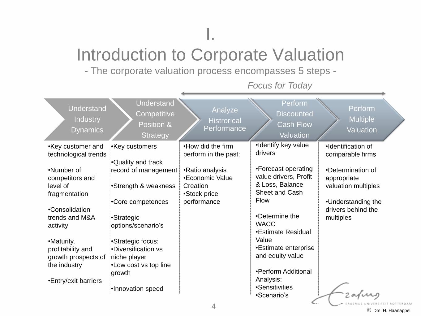
I.
Introduction to Corporate Valuation - The corporate valuation process encompasses 5 steps -
Focus for Today
Understand
Industry
Dynamics
Understand
Competitive
Position &
Strategy
Analyze
Histrorical Performance
Perform
Discounted
Cash Flow
Valuation
Perform
Multiple
Valuation
•Key customer and
technological trends
•Number of
competitors and
level of
fragmentation
•Consolidation
trends and M&A
activity
•Maturity,
profitability and
growth prospects of
the industry
•Entry/exit barriers
•Key customers
•Quality and track
record of management
•Strength & weakness
•Core competences
•Strategic
options/scenario’s
•Strategic focus:
•Diversification vs
niche player
•Low cost vs top line
growth
•Innovation speed
•How did the firm
perform in the past:
•Ratio analysis
•Economic Value
Creation
•Stock price
performance
•Identify key value
drivers
•Forecast operating
value drivers, Profit
& Loss, Balance
Sheet and Cash
Flow
•Determine the
WACC
•Estimate Residual
Value
•Estimate enterprise
and equity value
•Perform Additional
Analysis:
•Sensitivities
•Scenario’s
•Identification of
comparable firms
•Determination of
appropriate
valuation multiples
•Understanding the
drivers behind the
multiples
© Drs. H. Haanappel 4
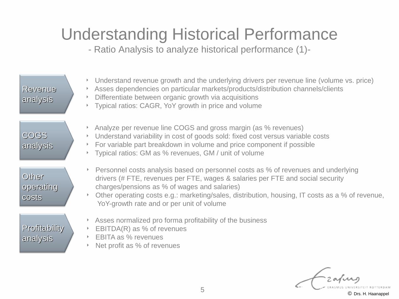
Understanding Historical Performance - Ratio Analysis to analyze historical performance (1)-
Revenue
analysis
Profitability
analysis
Other
operating
costs
COGS
analysis
‣ Understand revenue growth and the underlying drivers per revenue line (volume vs. price)
‣ Asses dependencies on particular markets/products/distribution channels/clients
‣ Differentiate between organic growth via acquisitions
‣ Typical ratios: CAGR, YoY growth in price and volume
‣ Analyze per revenue line COGS and gross margin (as % revenues)
‣ Understand variability in cost of goods sold: fixed cost versus variable costs
‣ For variable part breakdown in volume and price component if possible
‣ Typical ratios: GM as % revenues, GM / unit of volume
‣ Personnel costs analysis based on personnel costs as % of revenues and underlying
drivers (# FTE, revenues per FTE, wages & salaries per FTE and social security
charges/pensions as % of wages and salaries)
‣ Other operating costs e.g.: marketing/sales, distribution, housing, IT costs as a % of revenue,
YoY-growth rate and or per unit of volume
‣ Asses normalized pro forma profitability of the business
‣ EBITDA(R) as % of revenues
‣ EBITA as % revenues
‣ Net profit as % of revenues
© Drs. H. Haanappel 5
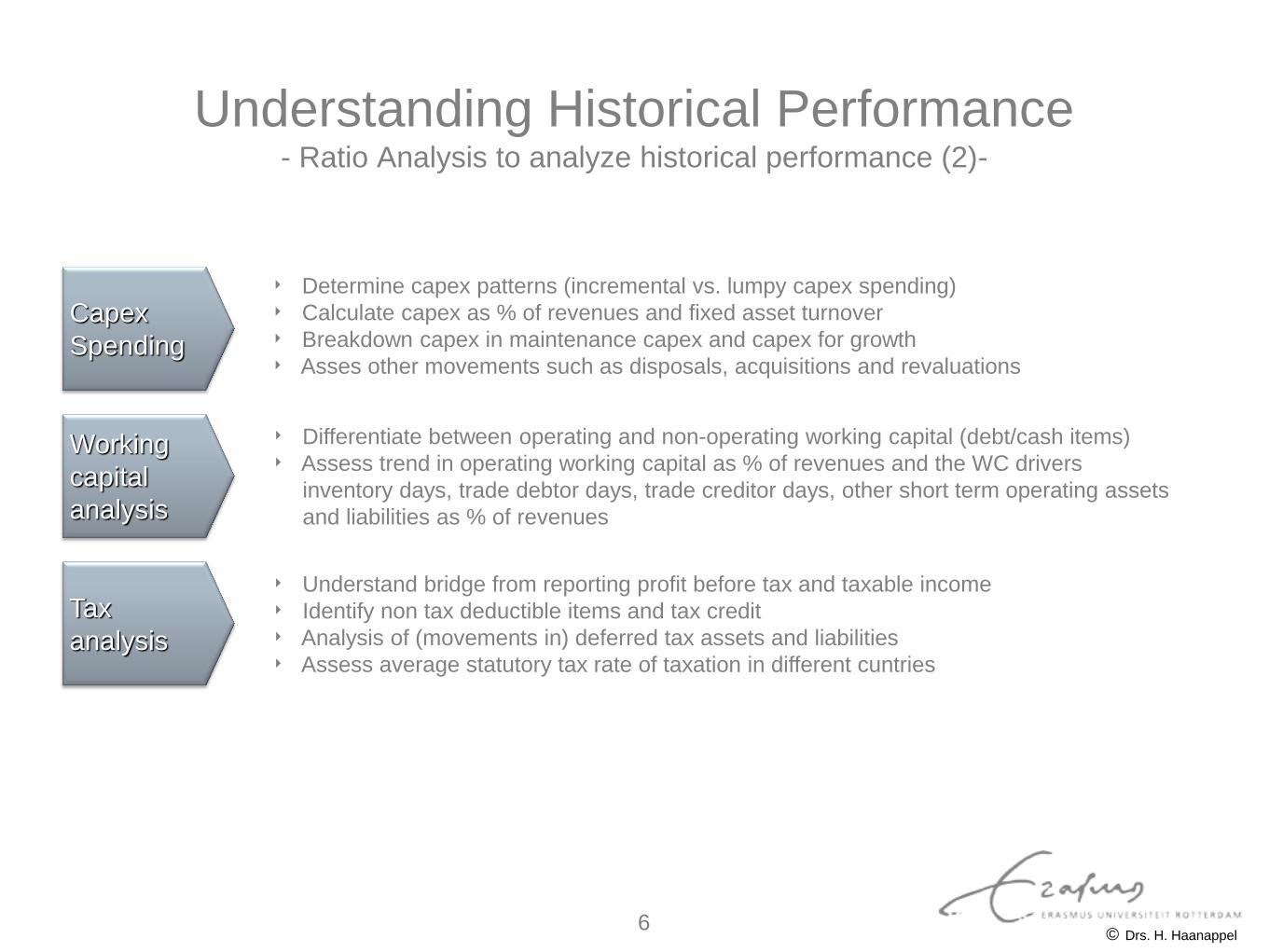
Understanding Historical Performance - Ratio Analysis to analyze historical performance (2)-
Capex
Spending
Tax
analysis
Working
capital
analysis
‣ Determine capex patterns (incremental vs. lumpy capex spending)
‣ Calculate capex as % of revenues and fixed asset turnover
‣ Breakdown capex in maintenance capex and capex for growth
‣ Asses other movements such as disposals, acquisitions and revaluations
‣ Differentiate between operating and non-operating working capital (debt/cash items)
‣ Assess trend in operating working capital as % of revenues and the WC drivers
inventory days, trade debtor days, trade creditor days, other short term operating assets
and liabilities as % of revenues
‣ Understand bridge from reporting profit before tax and taxable income
‣ Identify non tax deductible items and tax credit
‣ Analysis of (movements in) deferred tax assets and liabilities
‣ Assess average statutory tax rate of taxation in different cuntries
© Drs. H. Haanappel 6
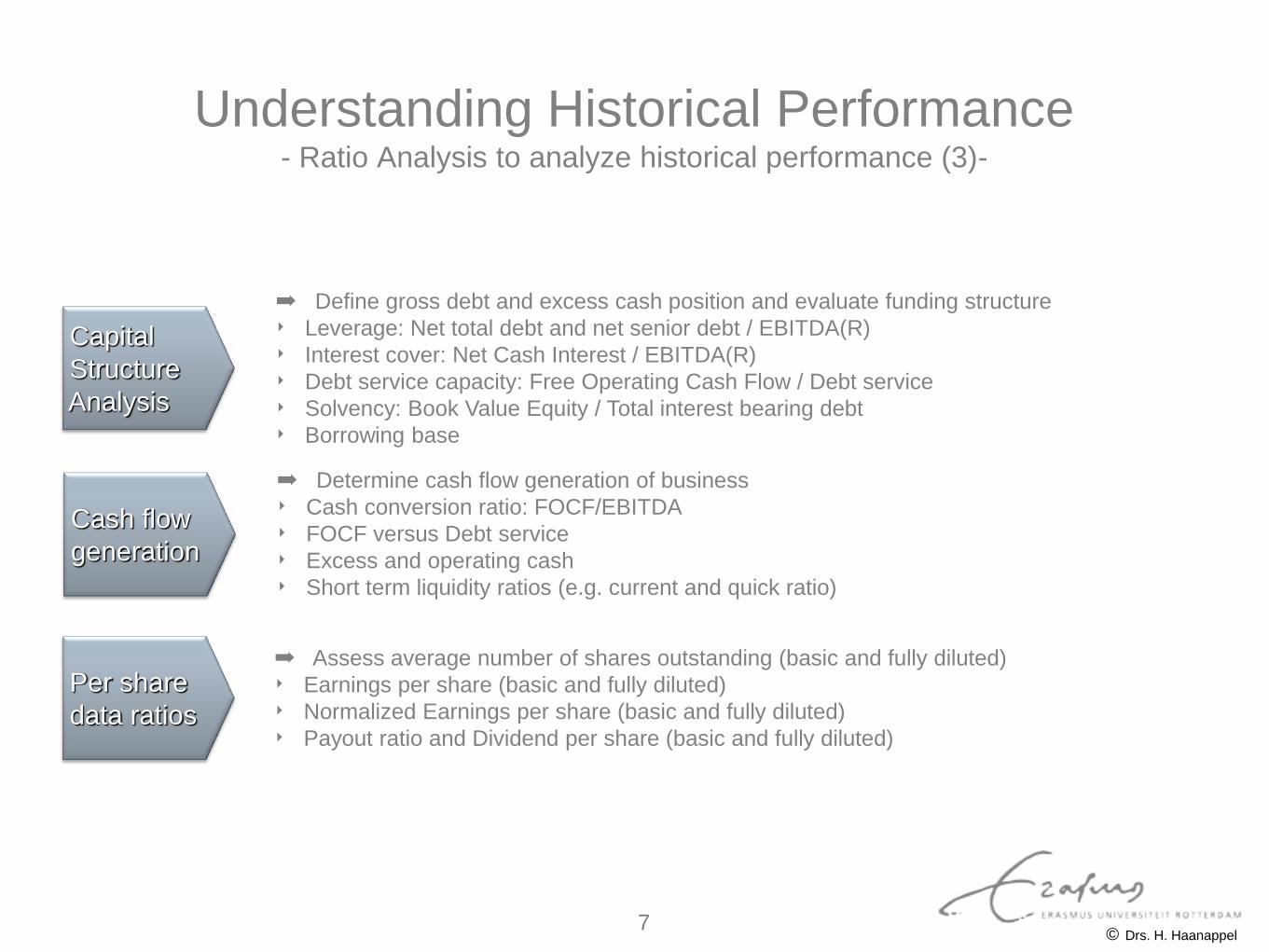
Understanding Historical Performance - Ratio Analysis to analyze historical performance (3)-
Capital
Structure
Analysis
Per share
data ratios
Cash flow
generation
➡ Define gross debt and excess cash position and evaluate funding structure
‣ Leverage: Net total debt and net senior debt / EBITDA(R)
‣ Interest cover: Net Cash Interest / EBITDA(R)
‣ Debt service capacity: Free Operating Cash Flow / Debt service
‣ Solvency: Book Value Equity / Total interest bearing debt
‣ Borrowing base
➡ Determine cash flow generation of business
‣ Cash conversion ratio: FOCF/EBITDA
‣ FOCF versus Debt service
‣ Excess and operating cash
‣ Short term liquidity ratios (e.g. current and quick ratio)
➡ Assess average number of shares outstanding (basic and fully diluted)
‣ Earnings per share (basic and fully diluted)
‣ Normalized Earnings per share (basic and fully diluted)
‣ Payout ratio and Dividend per share (basic and fully diluted)
© Drs. H. Haanappel 7
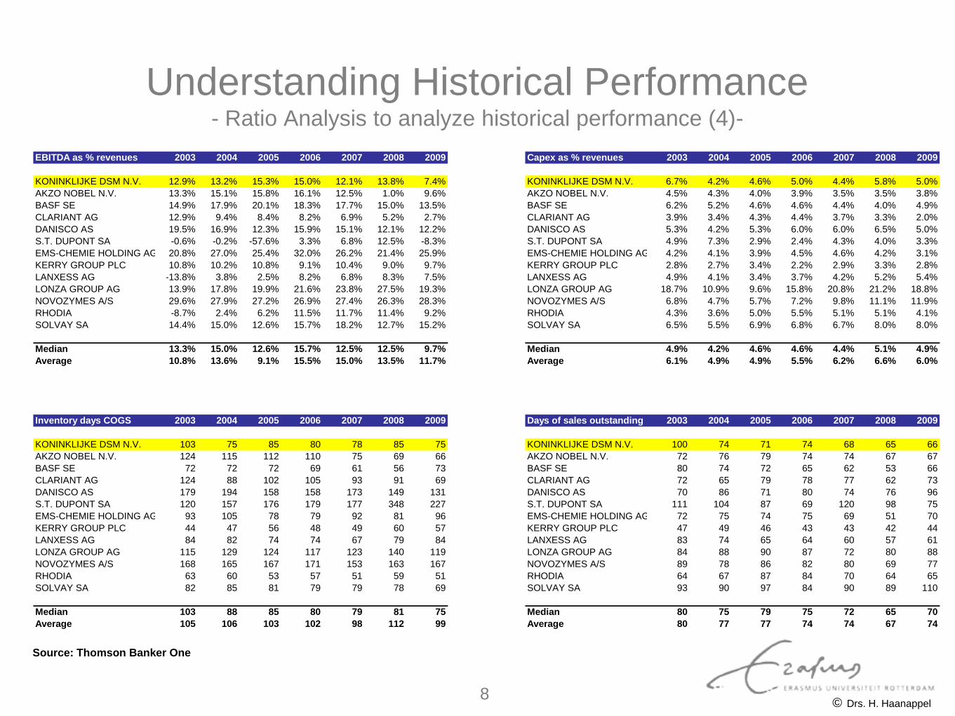
Understanding Historical Performance - Ratio Analysis to analyze historical performance (4)-
Capex as % revenues 2003 2004 2005 2006 2007 2008 2009
KONINKLIJKE DSM N.V. 6.7% 4.2% 4.6% 5.0% 4.4% 5.8% 5.0%
AKZO NOBEL N.V. 4.5% 4.3% 4.0% 3.9% 3.5% 3.5% 3.8%
BASF SE 6.2% 5.2% 4.6% 4.6% 4.4% 4.0% 4.9%
CLARIANT AG 3.9% 3.4% 4.3% 4.4% 3.7% 3.3% 2.0%
DANISCO AS 5.3% 4.2% 5.3% 6.0% 6.0% 6.5% 5.0%
S.T. DUPONT SA 4.9% 7.3% 2.9% 2.4% 4.3% 4.0% 3.3%
EMS-CHEMIE HOLDING AG 4.2% 4.1% 3.9% 4.5% 4.6% 4.2% 3.1%
KERRY GROUP PLC 2.8% 2.7% 3.4% 2.2% 2.9% 3.3% 2.8%
LANXESS AG 4.9% 4.1% 3.4% 3.7% 4.2% 5.2% 5.4%
LONZA GROUP AG 18.7% 10.9% 9.6% 15.8% 20.8% 21.2% 18.8%
NOVOZYMES A/S 6.8% 4.7% 5.7% 7.2% 9.8% 11.1% 11.9%
RHODIA 4.3% 3.6% 5.0% 5.5% 5.1% 5.1% 4.1%
SOLVAY SA 6.5% 5.5% 6.9% 6.8% 6.7% 8.0% 8.0%
Median 4.9% 4.2% 4.6% 4.6% 4.4% 5.1% 4.9%
Average 6.1% 4.9% 4.9% 5.5% 6.2% 6.6% 6.0%
EBITDA as % revenues 2003 2004 2005 2006 2007 2008 2009
KONINKLIJKE DSM N.V. 12.9% 13.2% 15.3% 15.0% 12.1% 13.8% 7.4%
AKZO NOBEL N.V. 13.3% 15.1% 15.8% 16.1% 12.5% 1.0% 9.6%
BASF SE 14.9% 17.9% 20.1% 18.3% 17.7% 15.0% 13.5%
CLARIANT AG 12.9% 9.4% 8.4% 8.2% 6.9% 5.2% 2.7%
DANISCO AS 19.5% 16.9% 12.3% 15.9% 15.1% 12.1% 12.2%
S.T. DUPONT SA -0.6% -0.2% -57.6% 3.3% 6.8% 12.5% -8.3%
EMS-CHEMIE HOLDING AG 20.8% 27.0% 25.4% 32.0% 26.2% 21.4% 25.9%
KERRY GROUP PLC 10.8% 10.2% 10.8% 9.1% 10.4% 9.0% 9.7%
LANXESS AG -13.8% 3.8% 2.5% 8.2% 6.8% 8.3% 7.5%
LONZA GROUP AG 13.9% 17.8% 19.9% 21.6% 23.8% 27.5% 19.3%
NOVOZYMES A/S 29.6% 27.9% 27.2% 26.9% 27.4% 26.3% 28.3%
RHODIA -8.7% 2.4% 6.2% 11.5% 11.7% 11.4% 9.2%
SOLVAY SA 14.4% 15.0% 12.6% 15.7% 18.2% 12.7% 15.2%
Median 13.3% 15.0% 12.6% 15.7% 12.5% 12.5% 9.7%
Average 10.8% 13.6% 9.1% 15.5% 15.0% 13.5% 11.7%
Inventory days COGS 2003 2004 2005 2006 2007 2008 2009
KONINKLIJKE DSM N.V. 103 75 85 80 78 85 75
AKZO NOBEL N.V. 124 115 112 110 75 69 66
BASF SE 72 72 72 69 61 56 73
CLARIANT AG 124 88 102 105 93 91 69
DANISCO AS 179 194 158 158 173 149 131
S.T. DUPONT SA 120 157 176 179 177 348 227
EMS-CHEMIE HOLDING AG 93 105 78 79 92 81 96
KERRY GROUP PLC 44 47 56 48 49 60 57
LANXESS AG 84 82 74 74 67 79 84
LONZA GROUP AG 115 129 124 117 123 140 119
NOVOZYMES A/S 168 165 167 171 153 163 167
RHODIA 63 60 53 57 51 59 51
SOLVAY SA 82 85 81 79 79 78 69
Median 103 88 85 80 79 81 75
Average 105 106 103 102 98 112 99
Days of sales outstanding 2003 2004 2005 2006 2007 2008 2009
KONINKLIJKE DSM N.V. 100 74 71 74 68 65 66
AKZO NOBEL N.V. 72 76 79 74 74 67 67
BASF SE 80 74 72 65 62 53 66
CLARIANT AG 72 65 79 78 77 62 73
DANISCO AS 70 86 71 80 74 76 96
S.T. DUPONT SA 111 104 87 69 120 98 75
EMS-CHEMIE HOLDING AG 72 75 74 75 69 51 70
KERRY GROUP PLC 47 49 46 43 43 42 44
LANXESS AG 83 74 65 64 60 57 61
LONZA GROUP AG 84 88 90 87 72 80 88
NOVOZYMES A/S 89 78 86 82 80 69 77
RHODIA 64 67 87 84 70 64 65
SOLVAY SA 93 90 97 84 90 89 110
Median 80 75 79 75 72 65 70
Average 80 77 77 74 74 67 74
Source: Thomson Banker One
© Drs. H. Haanappel 8
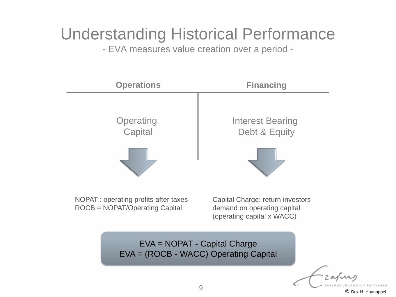
Understanding Historical Performance - EVA measures value creation over a period -
Operating
Capital
Interest Bearing
Debt & Equity
Operations Financing
NOPAT : operating profits after taxes
ROCB = NOPAT/Operating Capital
Capital Charge: return investors
demand on operating capital
(operating capital x WACC)
EVA = NOPAT - Capital Charge
EVA = (ROCB - WACC) Operating Capital
© Drs. H. Haanappel 9
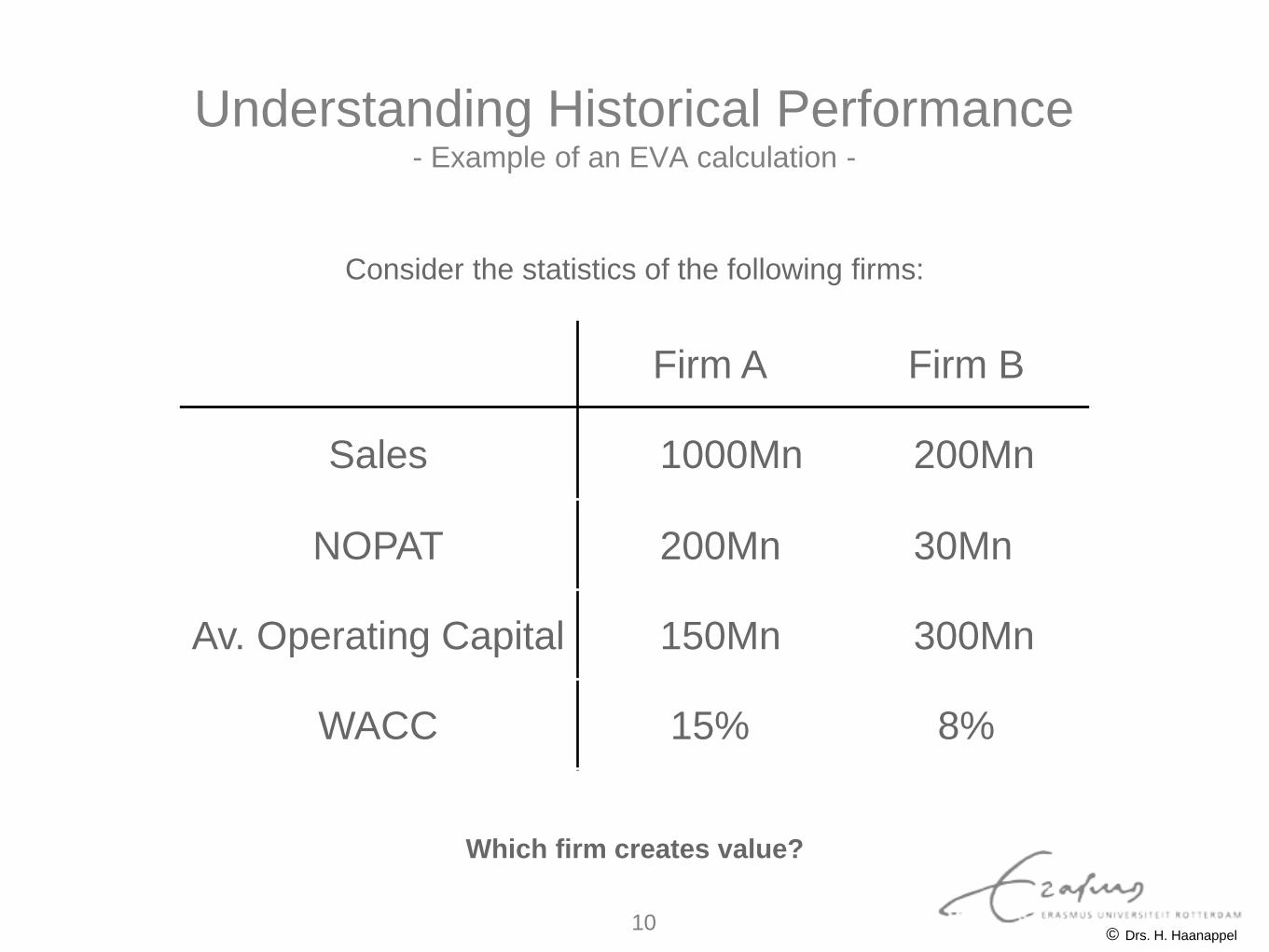
Understanding Historical Performance - Example of an EVA calculation -
Firm A Firm B
Sales 1000Mn 200Mn
NOPAT 200Mn 30Mn
Av. Operating Capital 150Mn 300Mn
WACC 15% 8%
Which firm creates value?
Consider the statistics of the following firms:
© Drs. H. Haanappel 10
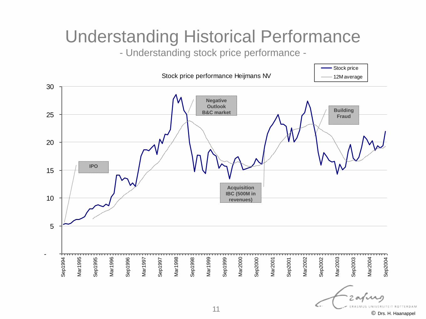
Understanding Historical Performance - Understanding stock price performance -
Stock price performance Heijmans NV
-
5
10
15
20
25
30
Sep1994
Mar1
995
Sep1995
Mar1
996
Sep1996
Mar1
997
Sep1997
Mar1
998
Sep1998
Mar1
999
Sep1999
Mar2
000
Sep2000
Mar2
001
Sep2001
Mar2
002
Sep2002
Mar2
003
Sep2003
Mar2
004
Sep2004
Stock price
12M average
IPO
Negative
Outlook
B&C market
Acquisition
IBC (500M in
revenues)
Building
Fraud
© Drs. H. Haanappel 11
II.
Corporate Valuation Using DCF-Framework - Value is determined by E (Cash flows) and Cost of Capital -
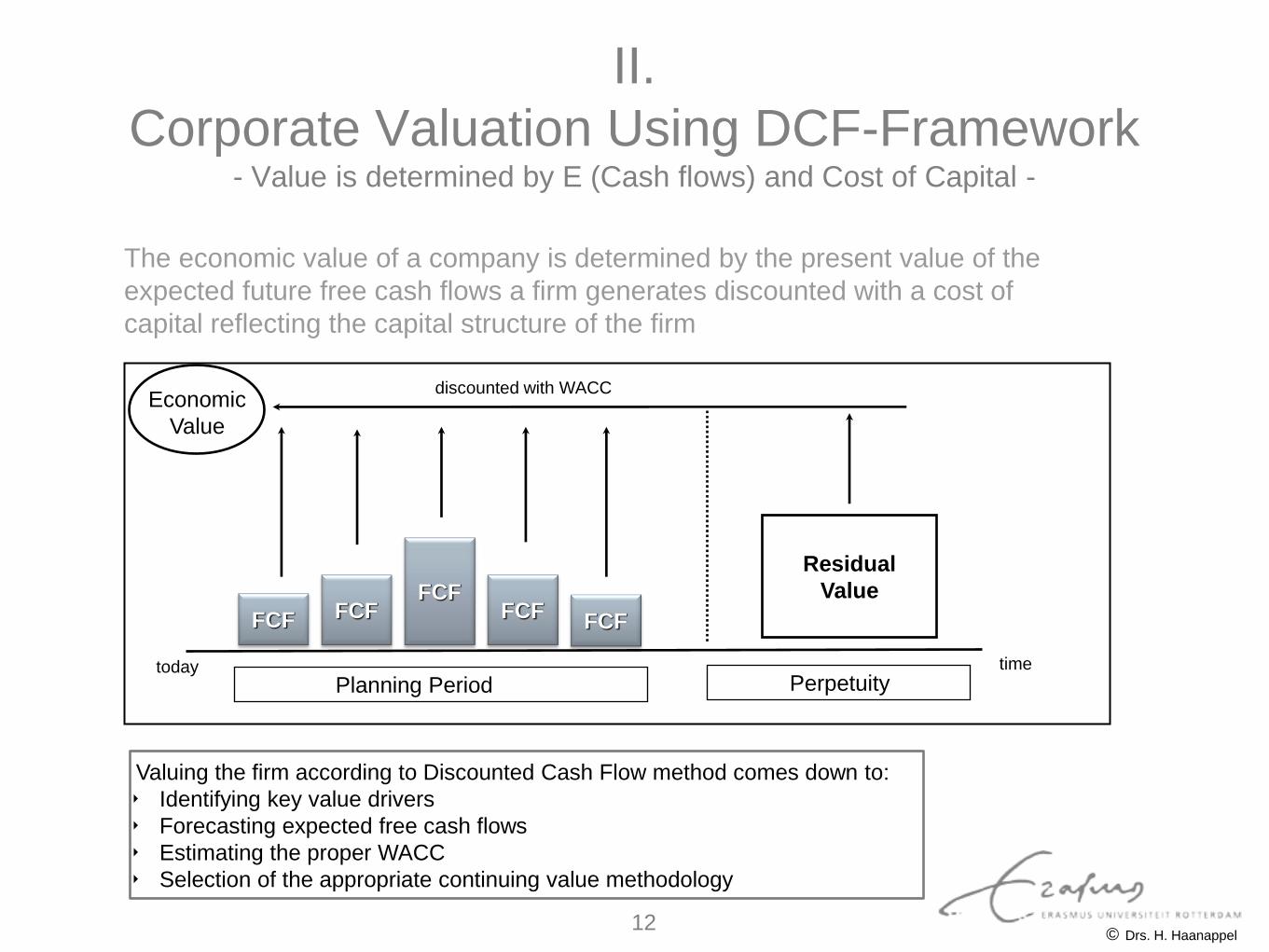
The economic value of a company is determined by the present value of the
expected future free cash flows a firm generates discounted with a cost of
capital reflecting the capital structure of the firm
Economic
Value
discounted with WACC
today time
FCF FCF
FCF FCF FCF
Planning Period Perpetuity
Residual
Value
Valuing the firm according to Discounted Cash Flow method comes down to:
‣ Identifying key value drivers
‣ Forecasting expected free cash flows
‣ Estimating the proper WACC
‣ Selection of the appropriate continuing value methodology
© Drs. H. Haanappel 12

Corporate Valuation Using DCF-Framework - Key value drivers determine E (Cash Flow) and Cost of Capital -
Net turnoverNet turnover
Cost of
goods sold
Cost of
goods sold
Gross marginGross margin
Operating
costs
Operating
costs
Personnel
costs
Personnel
costs
Other OpexOther Opex
Operating
profit
Operating
profit
Operating
Taxes
Operating
Taxes
NOPATNOPAT
Investments
NWC
Investments
NWC
Investments
fixed assets
Investments
fixed assets
Inventory
Turnover
Inventory
Turnover
Debtor daysDebtor days
Creditor daysCreditor days
Other current
assets/liabilities
Other current
assets/liabilities
Asset tunoverAsset tunover
Investments
Intangibles
Investments
Intangibles
InvestmentsInvestments
Free Cash FlowFree Cash Flow
Asset Utilization
Operating profitability
Business RiskBusiness Risk Capital StructureCapital Structure
Cost of equityCost of equity Cost of debtCost of debt
Tax rateTax rate
Tax rateTax rateCost of CapitalCost of Capital
Risk and capital structure
ECONOMIC
VALUE
ECONOMIC
VALUE
Operating value drivers:
• sales price per client
• discounts per client
• retention rate of clients
• net turnover per FTE
• material cost per unit
• transportation cost per unit
• manufacturing cost per unit
• production cycles
• energy cost per unit
• overhead/manufacturing fte
• salary per fte
• inventory turnover
• raw materials
• finished goods
• debtor days
• creditor days
• asset turnover
• tax rate
• investments in intangibles
© Drs. H. Haanappel 13
Corporate Valuation Using DCF-Framework - Definition of Free Cash Flow -
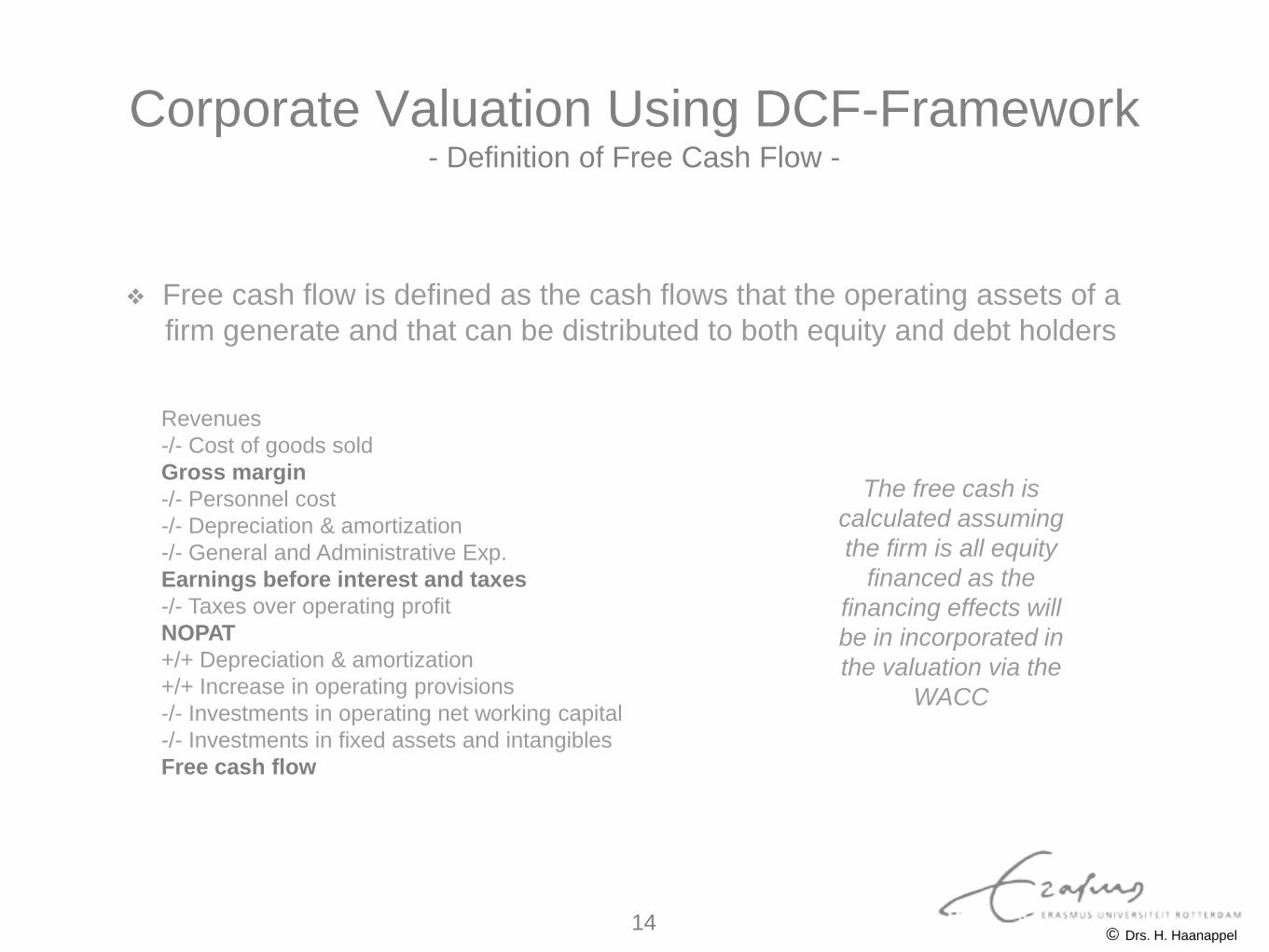
❖ Free cash flow is defined as the cash flows that the operating assets of a
firm generate and that can be distributed to both equity and debt holders
The free cash is
calculated assuming
the firm is all equity
financed as the
financing effects will
be in incorporated in
the valuation via the
WACC
Revenues
-/- Cost of goods sold
Gross margin
-/- Personnel cost
-/- Depreciation & amortization
-/- General and Administrative Exp.
Earnings before interest and taxes
-/- Taxes over operating profit
NOPAT
+/+ Depreciation & amortization
+/+ Increase in operating provisions
-/- Investments in operating net working capital
-/- Investments in fixed assets and intangibles
Free cash flow
© Drs. H. Haanappel 14
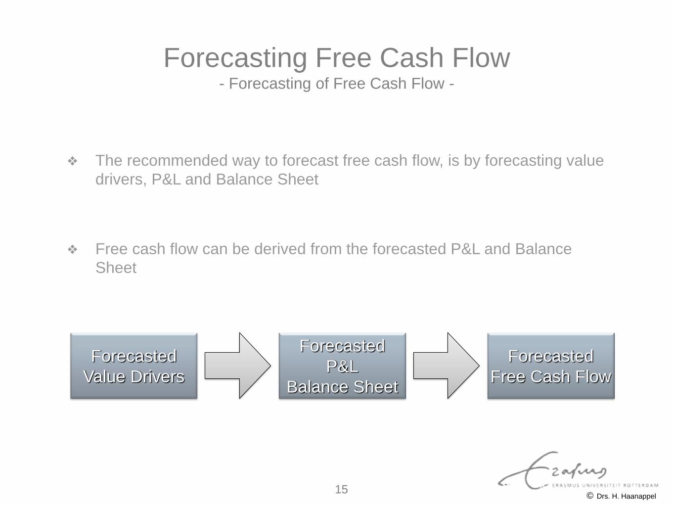
❖ The recommended way to forecast free cash flow, is by forecasting value
drivers, P&L and Balance Sheet
❖ Free cash flow can be derived from the forecasted P&L and Balance
Sheet
Forecasting Free Cash Flow - Forecasting of Free Cash Flow -
Forecasted
Value Drivers
Forecasted
P&L
Balance Sheet
Forecasted
Free Cash Flow
© Drs. H. Haanappel 15
Forecasting Free Cash Flow - Example of Forecast of Value Drivers -
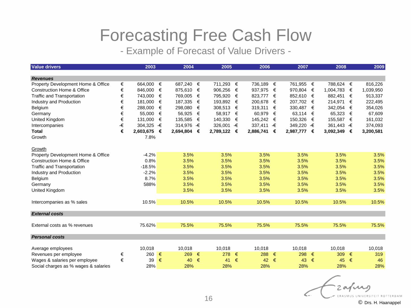
Value drivers 2003 2004 2005 2006 2007 2008 2009
Revenues
Property Development Home & Office 664,000€ 687,240€ 711,293€ 736,189€ 761,955€ 788,624€ 816,226€
Construction Home & Office 846,000€ 875,610€ 906,256€ 937,975€ 970,804€ 1,004,783€ 1,039,950€
Traffic and Transportation 743,000€ 769,005€ 795,920€ 823,777€ 852,610€ 882,451€ 913,337€
Industry and Production 181,000€ 187,335€ 193,892€ 200,678€ 207,702€ 214,971€ 222,495€
Belgium 288,000€ 298,080€ 308,513€ 319,311€ 330,487€ 342,054€ 354,026€
Germany 55,000€ 56,925€ 58,917€ 60,979€ 63,114€ 65,323€ 67,609€
United Kingdom 131,000€ 135,585€ 140,330€ 145,242€ 150,326€ 155,587€ 161,032€
Intercompanies 304,325-€ 314,976-€ 326,001-€ 337,411-€ 349,220-€ 361,443-€ 374,093-€
Total 2,603,675€ 2,694,804€ 2,789,122€ 2,886,741€ 2,987,777€ 3,092,349€ 3,200,581€
Growth 7.8%
Growth
Property Development Home & Office -4.2% 3.5% 3.5% 3.5% 3.5% 3.5% 3.5%
Construction Home & Office 0.8% 3.5% 3.5% 3.5% 3.5% 3.5% 3.5%
Traffic and Transportation -18.5% 3.5% 3.5% 3.5% 3.5% 3.5% 3.5%
Industry and Production -2.2% 3.5% 3.5% 3.5% 3.5% 3.5% 3.5%
Belgium 8.7% 3.5% 3.5% 3.5% 3.5% 3.5% 3.5%
Germany 588% 3.5% 3.5% 3.5% 3.5% 3.5% 3.5%
United Kingdom 3.5% 3.5% 3.5% 3.5% 3.5% 3.5%
Intercompanies as % sales 10.5% 10.5% 10.5% 10.5% 10.5% 10.5% 10.5%
External costs
External costs as % revenues 75.62% 75.5% 75.5% 75.5% 75.5% 75.5% 75.5%
Personal costs
Average employees 10,018 10,018 10,018 10,018 10,018 10,018 10,018
Revenues per employee 260€ 269€ 278€ 288€ 298€ 309€ 319€
Wages & salaries per employee 39€ 40€ 41€ 42€ 43€ 45€ 46€
Social charges as % wages & salaries 28% 28% 28% 28% 28% 28% 28%
© Drs. H. Haanappel 16
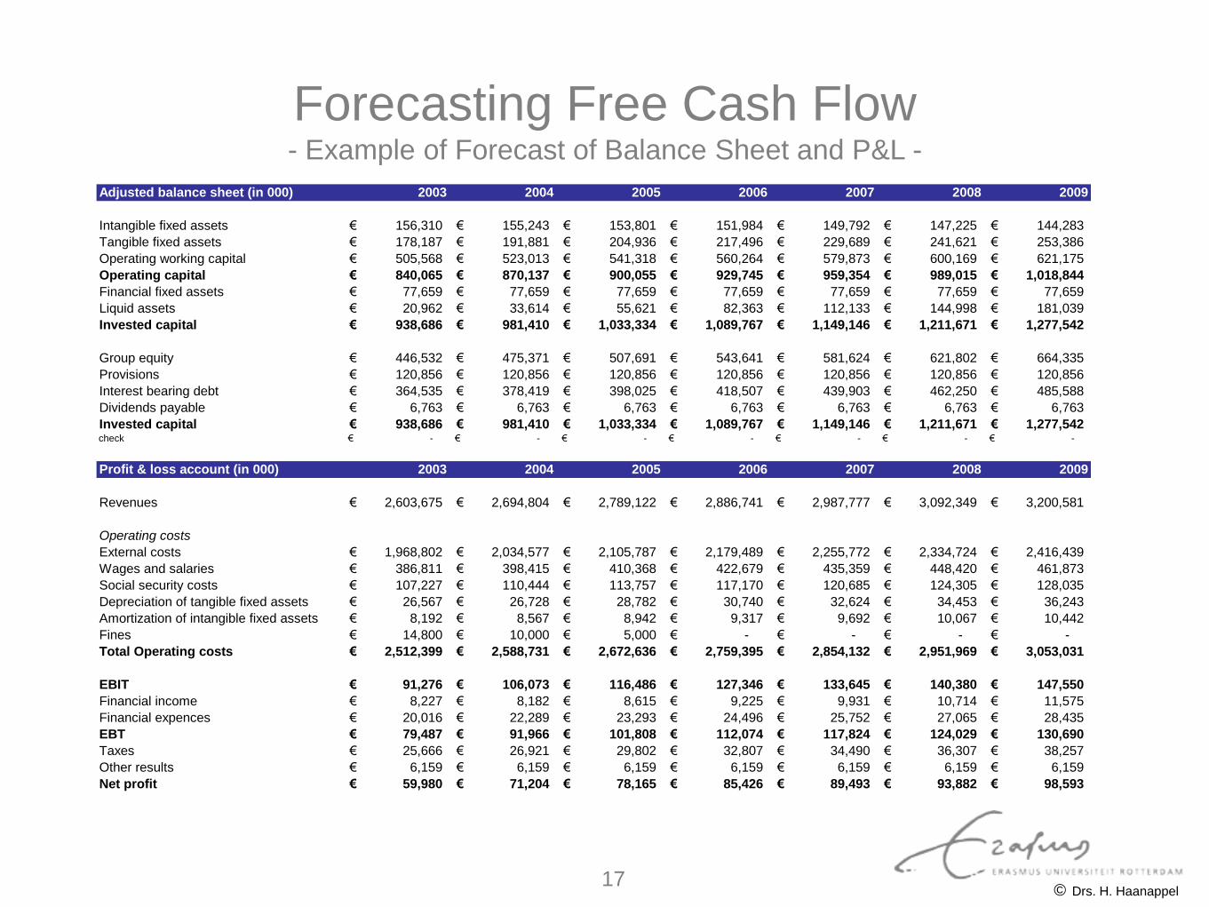
Forecasting Free Cash Flow - Example of Forecast of Balance Sheet and P&L -
Adjusted balance sheet (in 000) 2003 2004 2005 2006 2007 2008 2009
Intangible fixed assets 156,310€ 155,243€ 153,801€ 151,984€ 149,792€ 147,225€ 144,283€
Tangible fixed assets 178,187€ 191,881€ 204,936€ 217,496€ 229,689€ 241,621€ 253,386€
Operating working capital 505,568€ 523,013€ 541,318€ 560,264€ 579,873€ 600,169€ 621,175€
Operating capital 840,065€ 870,137€ 900,055€ 929,745€ 959,354€ 989,015€ 1,018,844€
Financial fixed assets 77,659€ 77,659€ 77,659€ 77,659€ 77,659€ 77,659€ 77,659€
Liquid assets 20,962€ 33,614€ 55,621€ 82,363€ 112,133€ 144,998€ 181,039€
Invested capital 938,686€ 981,410€ 1,033,334€ 1,089,767€ 1,149,146€ 1,211,671€ 1,277,542€
Group equity 446,532€ 475,371€ 507,691€ 543,641€ 581,624€ 621,802€ 664,335€
Provisions 120,856€ 120,856€ 120,856€ 120,856€ 120,856€ 120,856€ 120,856€
Interest bearing debt 364,535€ 378,419€ 398,025€ 418,507€ 439,903€ 462,250€ 485,588€
Dividends payable 6,763€ 6,763€ 6,763€ 6,763€ 6,763€ 6,763€ 6,763€
Invested capital 938,686€ 981,410€ 1,033,334€ 1,089,767€ 1,149,146€ 1,211,671€ 1,277,542€ check -€ -€ -€ -€ -€ -€ -€
Profit & loss account (in 000) 2003 2004 2005 2006 2007 2008 2009
Revenues 2,603,675€ 2,694,804€ 2,789,122€ 2,886,741€ 2,987,777€ 3,092,349€ 3,200,581€
Operating costs
External costs 1,968,802€ 2,034,577€ 2,105,787€ 2,179,489€ 2,255,772€ 2,334,724€ 2,416,439€
Wages and salaries 386,811€ 398,415€ 410,368€ 422,679€ 435,359€ 448,420€ 461,873€
Social security costs 107,227€ 110,444€ 113,757€ 117,170€ 120,685€ 124,305€ 128,035€
Depreciation of tangible fixed assets 26,567€ 26,728€ 28,782€ 30,740€ 32,624€ 34,453€ 36,243€
Amortization of intangible fixed assets 8,192€ 8,567€ 8,942€ 9,317€ 9,692€ 10,067€ 10,442€
Fines 14,800€ 10,000€ 5,000€ -€ -€ -€ -€
Total Operating costs 2,512,399€ 2,588,731€ 2,672,636€ 2,759,395€ 2,854,132€ 2,951,969€ 3,053,031€
EBIT 91,276€ 106,073€ 116,486€ 127,346€ 133,645€ 140,380€ 147,550€
Financial income 8,227€ 8,182€ 8,615€ 9,225€ 9,931€ 10,714€ 11,575€
Financial expences 20,016€ 22,289€ 23,293€ 24,496€ 25,752€ 27,065€ 28,435€
EBT 79,487€ 91,966€ 101,808€ 112,074€ 117,824€ 124,029€ 130,690€
Taxes 25,666€ 26,921€ 29,802€ 32,807€ 34,490€ 36,307€ 38,257€
Other results 6,159€ 6,159€ 6,159€ 6,159€ 6,159€ 6,159€ 6,159€
Net profit 59,980€ 71,204€ 78,165€ 85,426€ 89,493€ 93,882€ 98,593€
© Drs. H. Haanappel 17
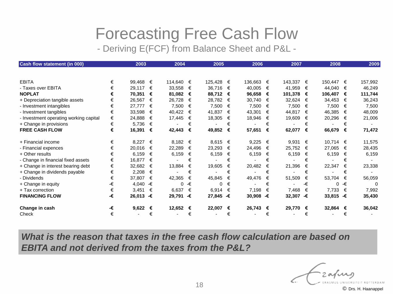
Forecasting Free Cash Flow - Deriving E(FCF) from Balance Sheet and P&L -
Cash flow statement (in 000) 2003 2004 2005 2006 2007 2008 2009
EBITA 99,468€ 114,640€ 125,428€ 136,663€ 143,337€ 150,447€ 157,992€
- Taxes over EBITA 29,117€ 33,558€ 36,716€ 40,005€ 41,959€ 44,040€ 46,249€
NOPLAT 70,351€ 81,082€ 88,712€ 96,658€ 101,378€ 106,407€ 111,744€
+ Depreciation tangible assets 26,567€ 26,728€ 28,782€ 30,740€ 32,624€ 34,453€ 36,243€
- Investment intangibles 27,777€ 7,500€ 7,500€ 7,500€ 7,500€ 7,500€ 7,500€
- Investment tangibles 33,598€ 40,422€ 41,837€ 43,301€ 44,817€ 46,385€ 48,009€
- Investment operating working capital 24,888€ 17,445€ 18,305€ 18,946€ 19,609€ 20,296€ 21,006€
+ Change in provisions 5,736€ -€ -€ -€ -€ -€ -€
FREE CASH FLOW 16,391€ 42,443€ 49,852€ 57,651€ 62,077€ 66,679€ 71,472€
+ Financial income 8,227€ 8,182€ 8,615€ 9,225€ 9,931€ 10,714€ 11,575€
- Financial expences 20,016€ 22,289€ 23,293€ 24,496€ 25,752€ 27,065€ 28,435€
+ Other results 6,159€ 6,159€ 6,159€ 6,159€ 6,159€ 6,159€ 6,159€
- Change in financial fixed assets 16,877€ -€ -€ -€ -€ -€ -€
+ Change in interest bearing debt 32,682€ 13,884€ 19,605€ 20,482€ 21,396€ 22,347€ 23,338€
+ Change in dividends payable 2,208€ -€ -€ -€ -€ -€ -€
- Dividends 37,807€ 42,365€ 45,845€ 49,476€ 51,509€ 53,704€ 56,059€
+ Change in equity 4,040-€ 0-€ 0-€ -€ -€ 0-€ 0-€
+ Tax correction 3,451€ 6,637€ 6,914€ 7,198€ 7,468€ 7,733€ 7,992€
FINANCING FLOW 26,013-€ 29,791-€ 27,845-€ 30,908-€ 32,307-€ 33,815-€ 35,430-€
Change in cash 9,622-€ 12,652€ 22,007€ 26,743€ 29,770€ 32,864€ 36,042€
Check -€ -€ -€ -€ -€ -€ -€
What is the reason that taxes in the free cash flow calculation are based on
EBITA and not derived from the taxes from the P&L?
© Drs. H. Haanappel 18
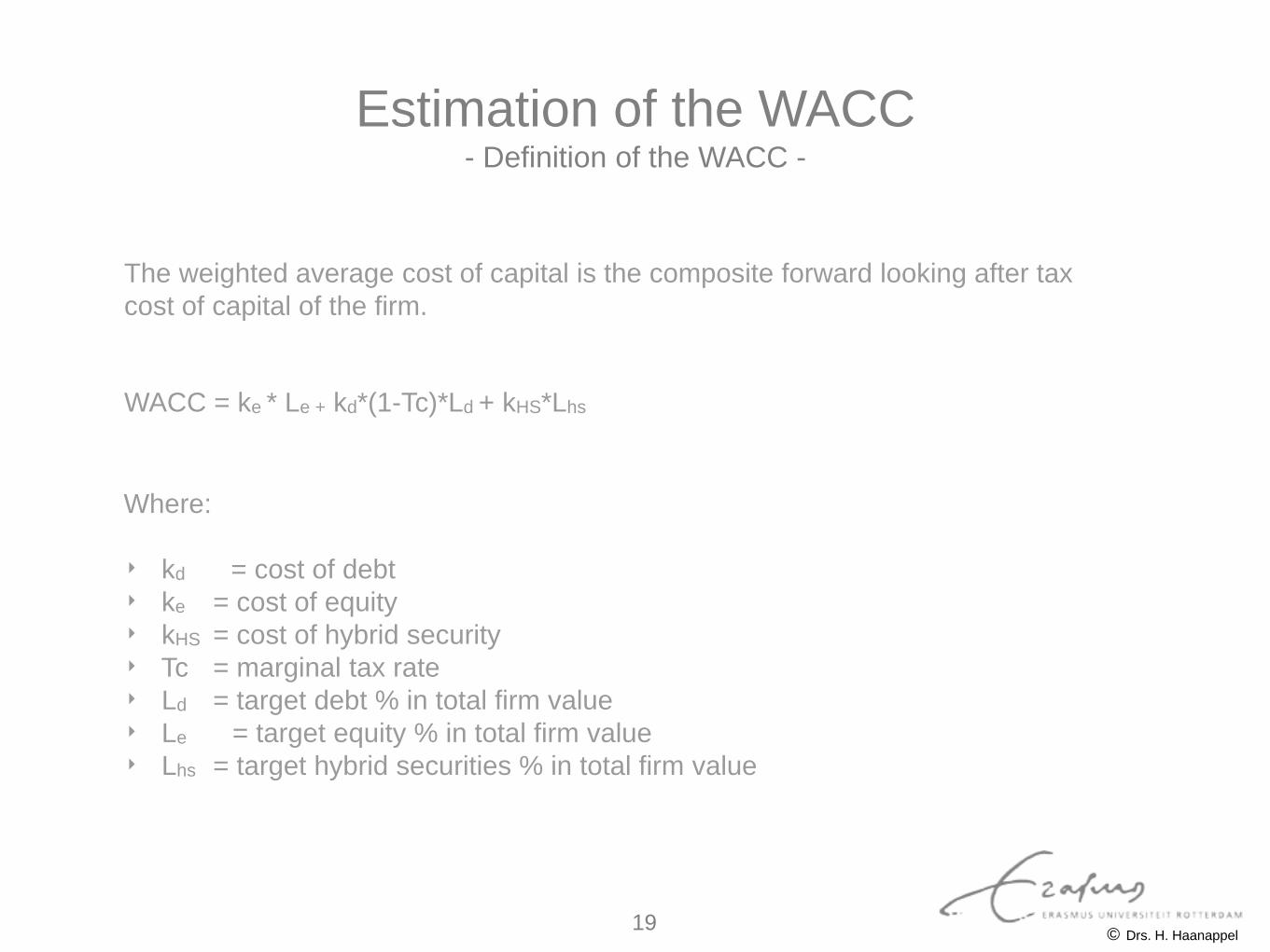
Estimation of the WACC - Definition of the WACC -
Where:
‣ kd = cost of debt
‣ ke = cost of equity
‣ kHS = cost of hybrid security
‣ Tc = marginal tax rate
‣ Ld = target debt % in total firm value
‣ Le = target equity % in total firm value
‣ Lhs = target hybrid securities % in total firm value
The weighted average cost of capital is the composite forward looking after tax
cost of capital of the firm.
WACC = ke * Le + kd*(1-Tc)*Ld + kHS*Lhs
© Drs. H. Haanappel 19
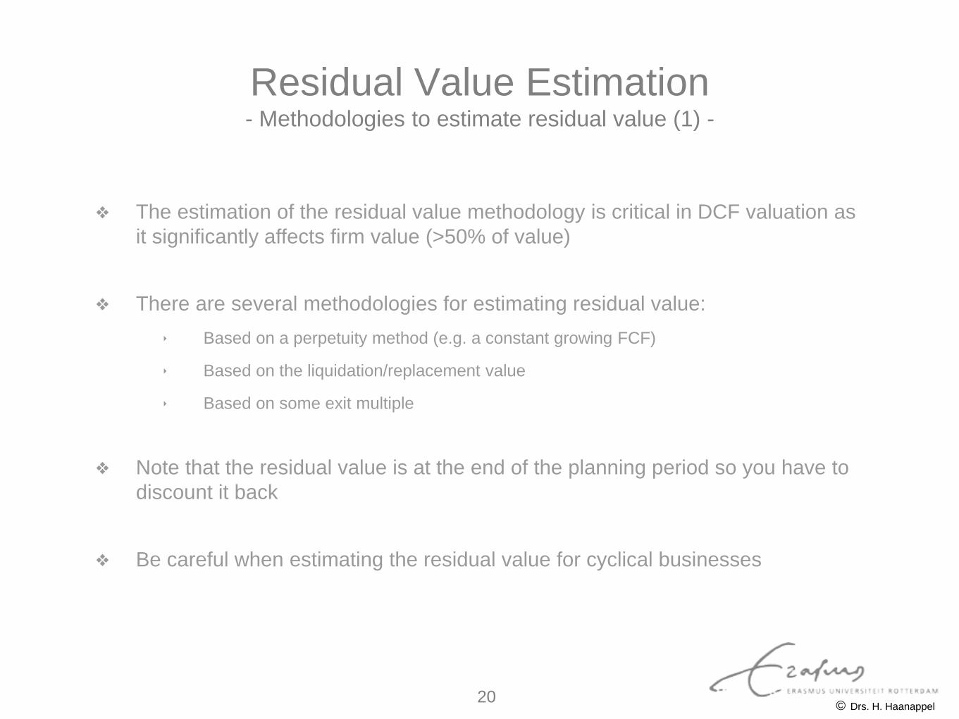
Residual Value Estimation - Methodologies to estimate residual value (1) -
❖ There are several methodologies for estimating residual value:
‣ Based on a perpetuity method (e.g. a constant growing FCF)
‣ Based on the liquidation/replacement value
‣ Based on some exit multiple
❖ Note that the residual value is at the end of the planning period so you have to
discount it back
❖ The estimation of the residual value methodology is critical in DCF valuation as
it significantly affects firm value (>50% of value)
❖ Be careful when estimating the residual value for cyclical businesses
© Drs. H. Haanappel 20
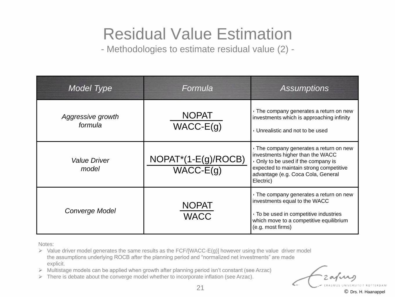
Residual Value Estimation - Methodologies to estimate residual value (2) -
Model Type Formula Assumptions
Aggressive growth
formula
NOPAT
WACC-E(g)
‣ The company generates a return on new
investments which is approaching infinity
‣ Unrealistic and not to be used
Value Driver
model
NOPAT*(1-E(g)/ROCB)
WACC-E(g)
‣ The company generates a return on new
investments higher than the WACC
‣ Only to be used if the company is
expected to maintain strong competitive
advantage (e.g. Coca Cola, General
Electric)
Converge Model NOPAT
WACC
‣ The company generates a return on new
investments equal to the WACC
‣ To be used in competitive industries
which move to a competitive equilibrium
(e.g. most firms)
Notes:
Value driver model generates the same results as the FCF/[WACC-E(g)] however using the value driver model
the assumptions underlying ROCB after the planning period and “normalized net investments” are made
explicit.
Multistage models can be applied when growth after planning period isn’t constant (see Arzac)
There is debate about the converge model whether to incorporate inflation (see Arzac).
© Drs. H. Haanappel 21
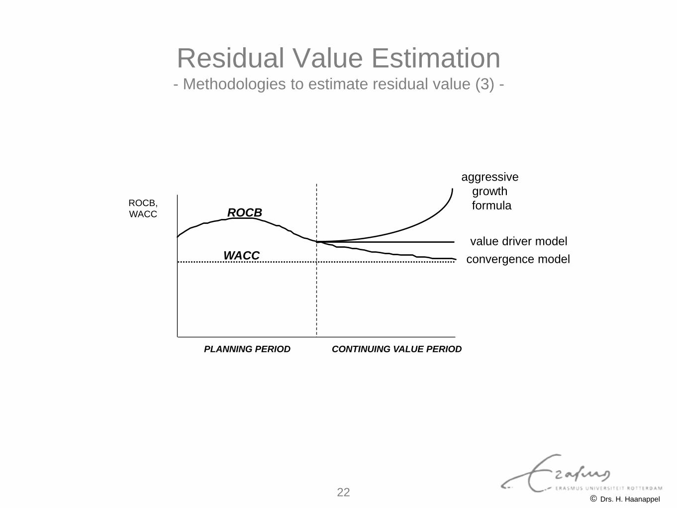
Residual Value Estimation - Methodologies to estimate residual value (3) -
WACC
PLANNING PERIOD CONTINUING VALUE PERIOD
value driver model
ROCB
aggressive
growth
formula
convergence model
ROCB,
WACC
© Drs. H. Haanappel 22
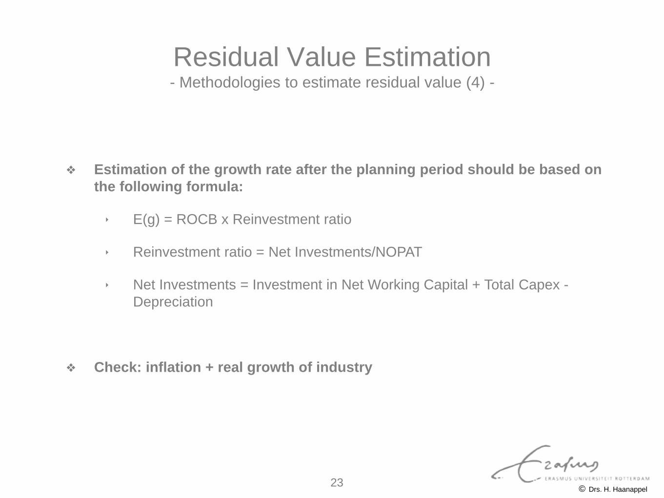
Residual Value Estimation - Methodologies to estimate residual value (4) -
❖ Estimation of the growth rate after the planning period should be based on
the following formula:
‣ E(g) = ROCB x Reinvestment ratio
‣ Reinvestment ratio = Net Investments/NOPAT
‣ Net Investments = Investment in Net Working Capital + Total Capex -
Depreciation
❖ Check: inflation + real growth of industry
© Drs. H. Haanappel 23
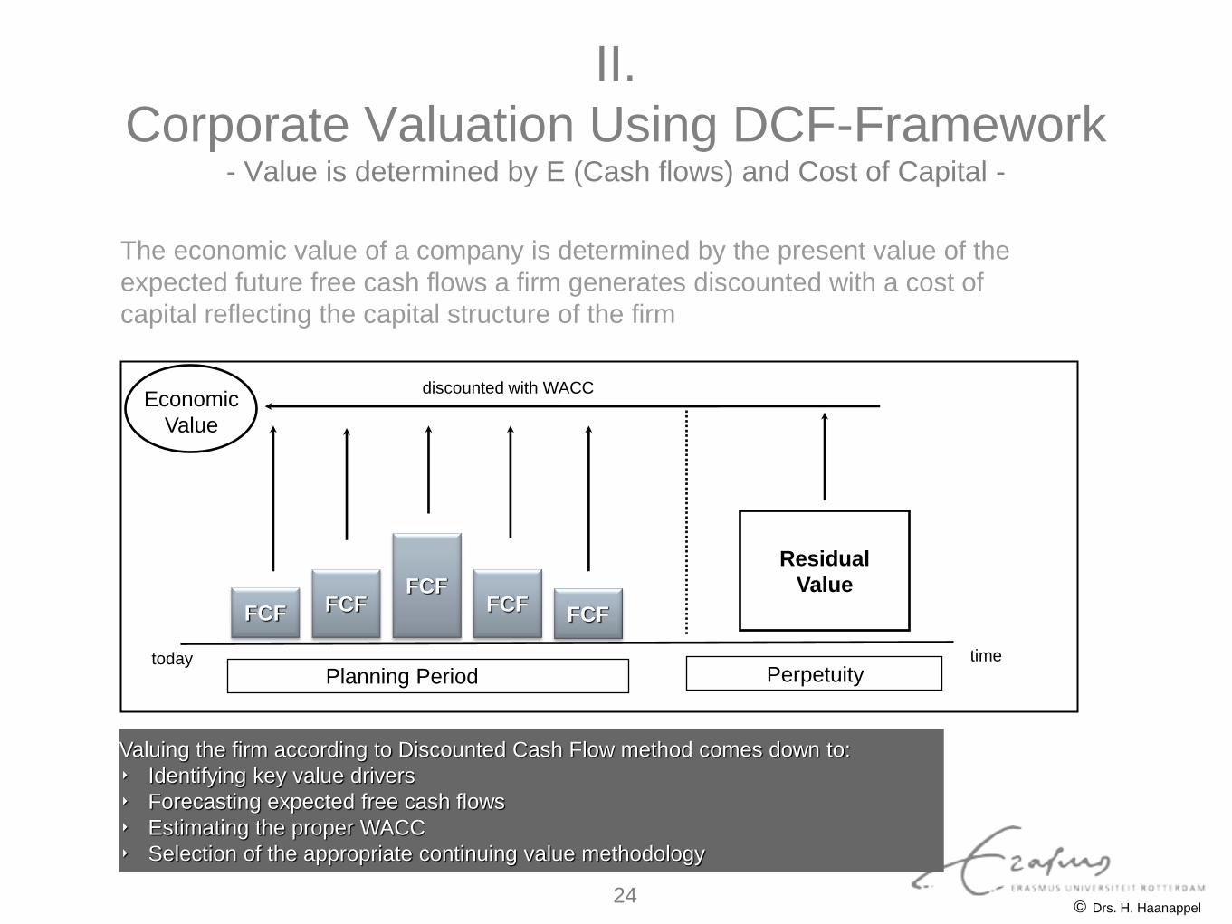
II.
Corporate Valuation Using DCF-Framework - Value is determined by E (Cash flows) and Cost of Capital -
The economic value of a company is determined by the present value of the
expected future free cash flows a firm generates discounted with a cost of
capital reflecting the capital structure of the firm
Economic
Value
discounted with WACC
today time
FCF FCF
FCF FCF FCF
Planning Period Perpetuity
Residual
Value
Valuing the firm according to Discounted Cash Flow method comes down to:
‣ Identifying key value drivers
‣ Forecasting expected free cash flows
‣ Estimating the proper WACC
‣ Selection of the appropriate continuing value methodology
© Drs. H. Haanappel 24
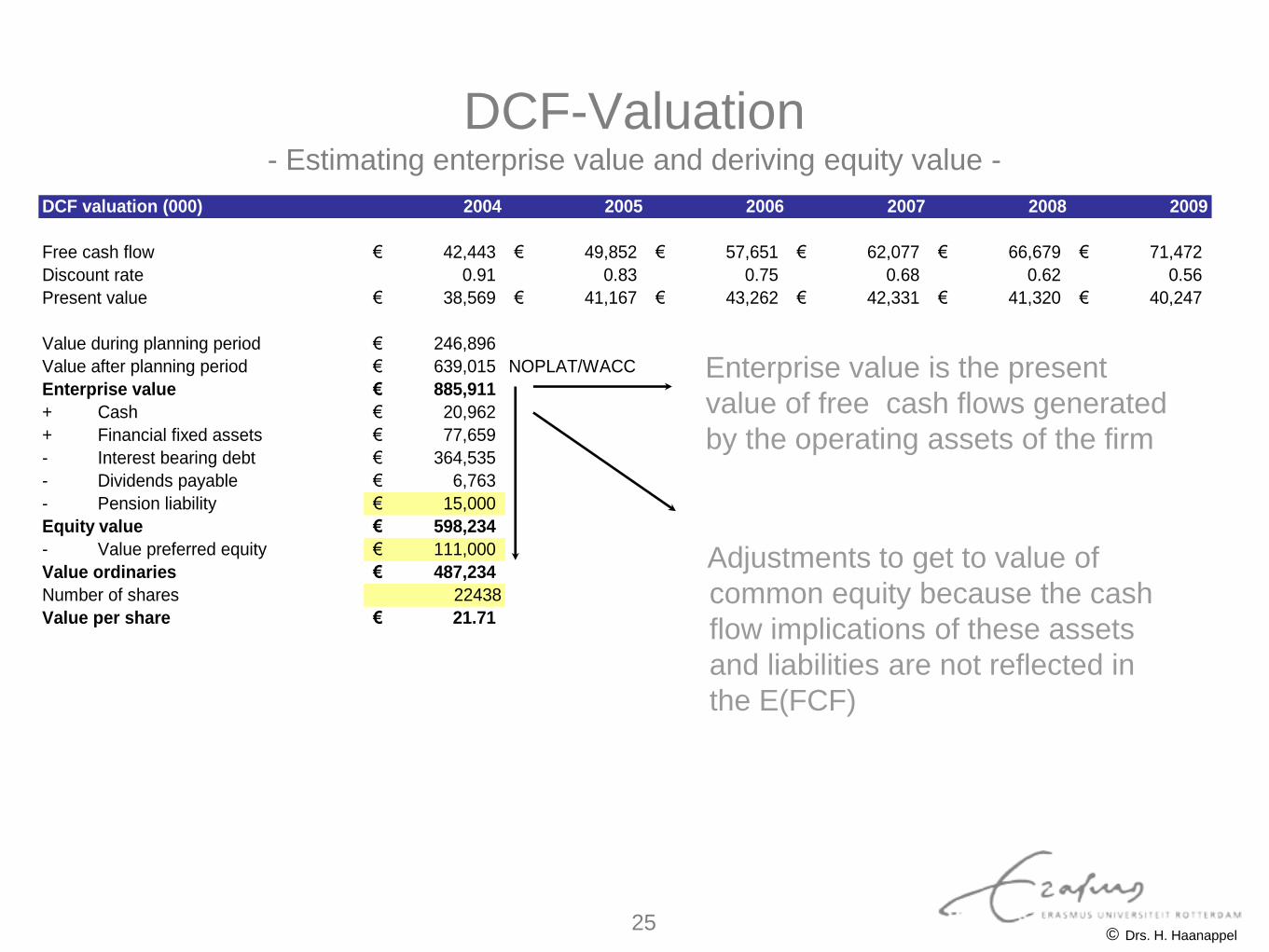
DCF-Valuation - Estimating enterprise value and deriving equity value -
Enterprise value is the present
value of free cash flows generated
by the operating assets of the firm
Adjustments to get to value of
common equity because the cash
flow implications of these assets
and liabilities are not reflected in
the E(FCF)
DCF valuation (000) 2004 2005 2006 2007 2008 2009
Free cash flow 42,443€ 49,852€ 57,651€ 62,077€ 66,679€ 71,472€
Discount rate 0.91 0.83 0.75 0.68 0.62 0.56
Present value 38,569€ 41,167€ 43,262€ 42,331€ 41,320€ 40,247€
Value during planning period 246,896€
Value after planning period 639,015€ NOPLAT/WACC
Enterprise value 885,911€
+ Cash 20,962€
+ Financial fixed assets 77,659€
- Interest bearing debt 364,535€
- Dividends payable 6,763€
- Pension liability 15,000€
Equity value 598,234€
- Value preferred equity 111,000€
Value ordinaries 487,234€
Number of shares 22438
Value per share 21.71€
© Drs. H. Haanappel 25
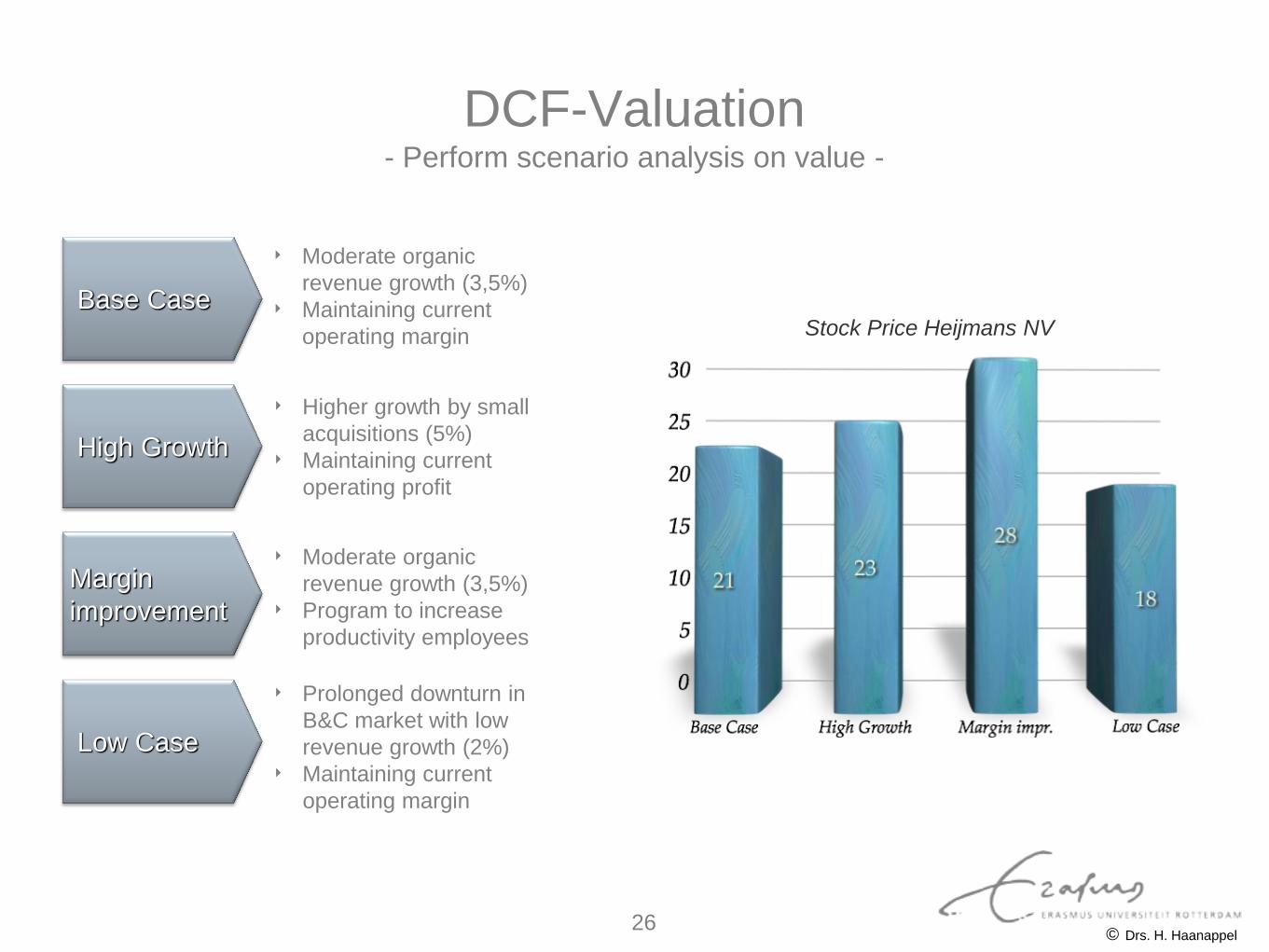
DCF-Valuation - Perform scenario analysis on value -
Base Case
Low Case
Margin
improvement
High Growth
‣ Moderate organic
revenue growth (3,5%)
‣ Maintaining current
operating margin
‣ Higher growth by small
acquisitions (5%)
‣ Maintaining current
operating profit
‣ Moderate organic
revenue growth (3,5%)
‣ Program to increase
productivity employees
‣ Prolonged downturn in
B&C market with low
revenue growth (2%)
‣ Maintaining current
operating margin
Stock Price Heijmans NV
© Drs. H. Haanappel 26
❖ There should be consistency with the discount rate and the cash flow
definition:
‣ Cash Flows to the firm vs cash flows to equity holders
‣ Real cash flows versus nominal cash flows
‣ Pretax cash flows versus after tax cash flows
‣ Dollar cash flows versus Euro cash flows
❖ There are alternative DCF-model available to value a firm, for example:
‣ Discounting the FCF to equity with the Cost of Equity (to be used when valuing financial
institutions)
‣ Discounting Dividends with the Cost of Equity (not used in practice a lot)
=> In practice one tends to use local currency nominal cash flows to the firm
DCF-Valuation - Final remarks DCF-Valuation -
© Drs. H. Haanappel 27
III.
Multiple Valuation - Principles about Valuation Multiples -
❖ Classifications of multiples:
‣ Trading Multiples
‣ Transaction Multiples
‣ Industry specific Multiples
‣ Historical Multiples
‣ Trailing Multiples
‣ Forward looking Multiples
❖ The valuation of an asset that is based on the prices currently being paid for
assets that are comparable:
‣ Similar risk profile
‣ Similar leverage
‣ Similar growth expectations
‣ Similar size
Based on current market capitalization
Based on pricing in M&A
Specific for the industry
Current price related to historical results
Current price related to last 12 months results
Current price related to analyst expectations
© Drs. H. Haanappel 28
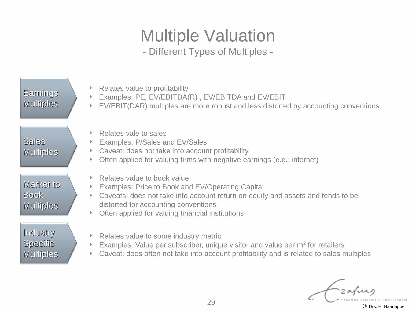
Multiple Valuation - Different Types of Multiples -
Earnings
Multiples
Industry
Specific
Multiples
Market to
Book
Multiples
Sales
Multiples
‣ Relates value to profitability
‣ Examples: PE, EV/EBITDA(R) , EV/EBITDA and EV/EBIT
‣ EV/EBIT(DAR) multiples are more robust and less distorted by accounting conventions
‣ Relates vale to sales
‣ Examples: P/Sales and EV/Sales
‣ Caveat: does not take into account profitability
‣ Often applied for valuing firms with negative earnings (e.g.: internet)
‣ Relates value to book value
‣ Examples: Price to Book and EV/Operating Capital
‣ Caveats: does not take into account return on equity and assets and tends to be
distorted for accounting conventions
‣ Often applied for valuing financial institutions
‣ Relates value to some industry metric
‣ Examples: Value per subscriber, unique visitor and value per m2 for retailers
‣ Caveat: does often not take into account profitability and is related to sales multiples
© Drs. H. Haanappel 29
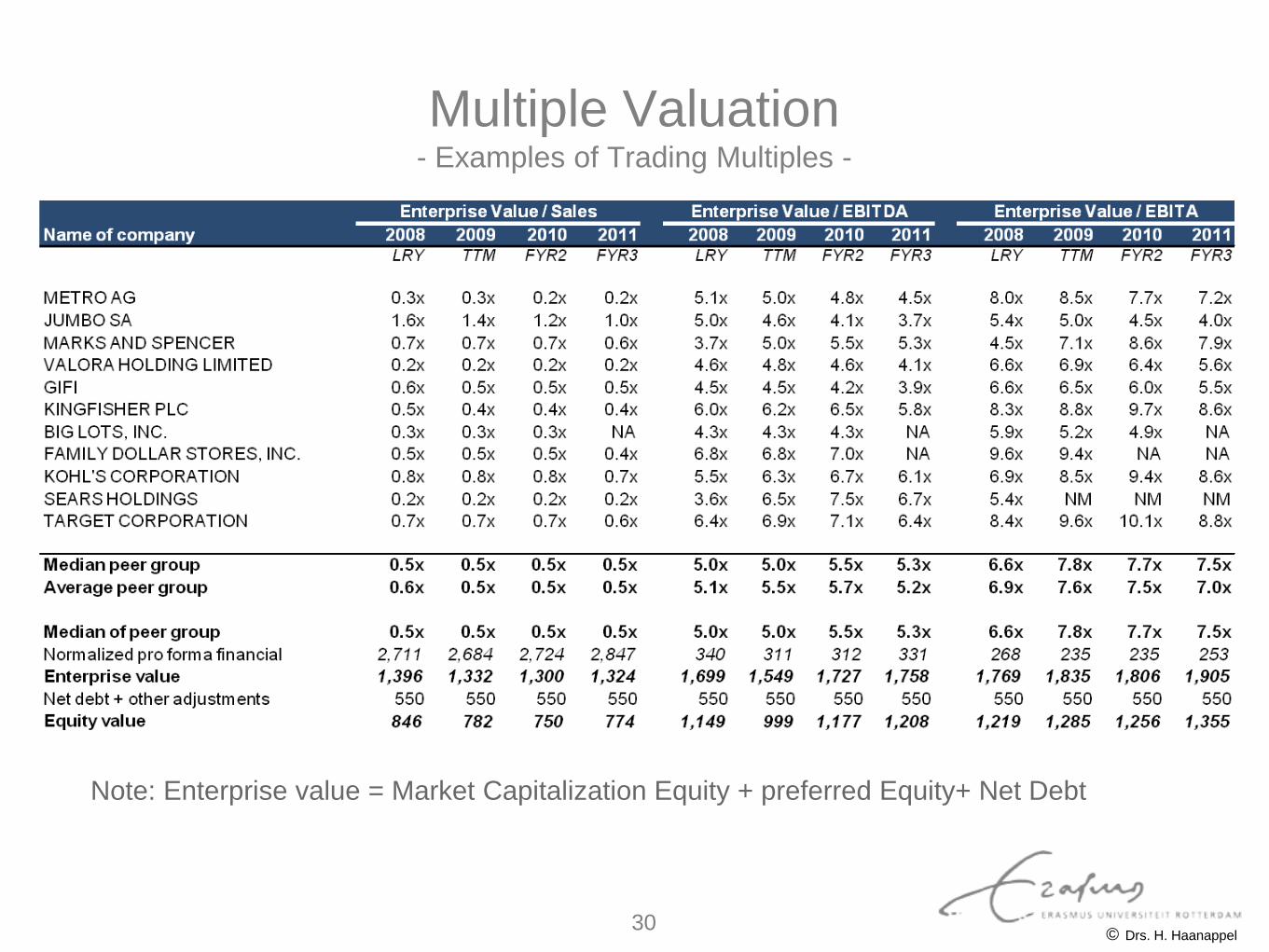
Multiple Valuation - Examples of Trading Multiples -
Note: Enterprise value = Market Capitalization Equity + preferred Equity+ Net Debt
© Drs. H. Haanappel 30
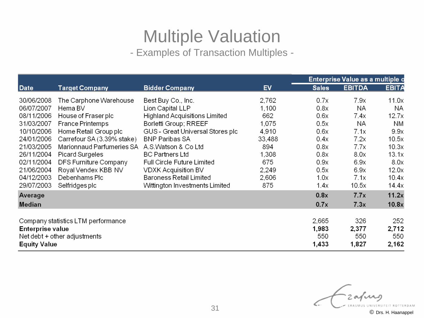
Multiple Valuation - Examples of Transaction Multiples -
© Drs. H. Haanappel 31
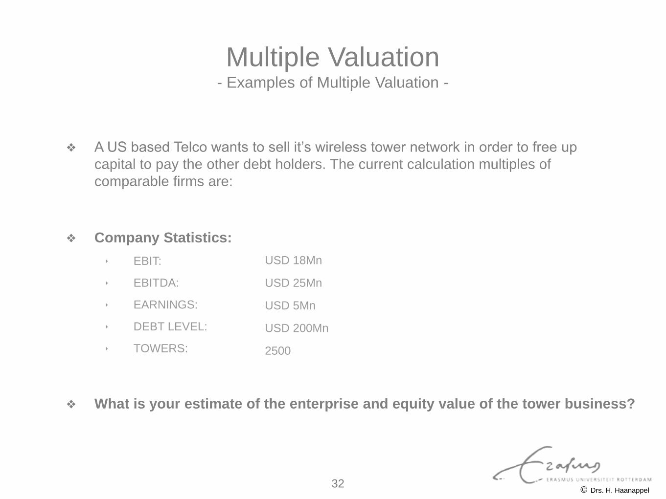
❖ Company Statistics:
‣ EBIT:
‣ EBITDA:
‣ EARNINGS:
‣ DEBT LEVEL:
‣ TOWERS:
❖ A US based Telco wants to sell it’s wireless tower network in order to free up
capital to pay the other debt holders. The current calculation multiples of
comparable firms are:
❖ What is your estimate of the enterprise and equity value of the tower business?
USD 18Mn
USD 25Mn
USD 5Mn
USD 200Mn
2500
Multiple Valuation - Examples of Multiple Valuation -
© Drs. H. Haanappel 32
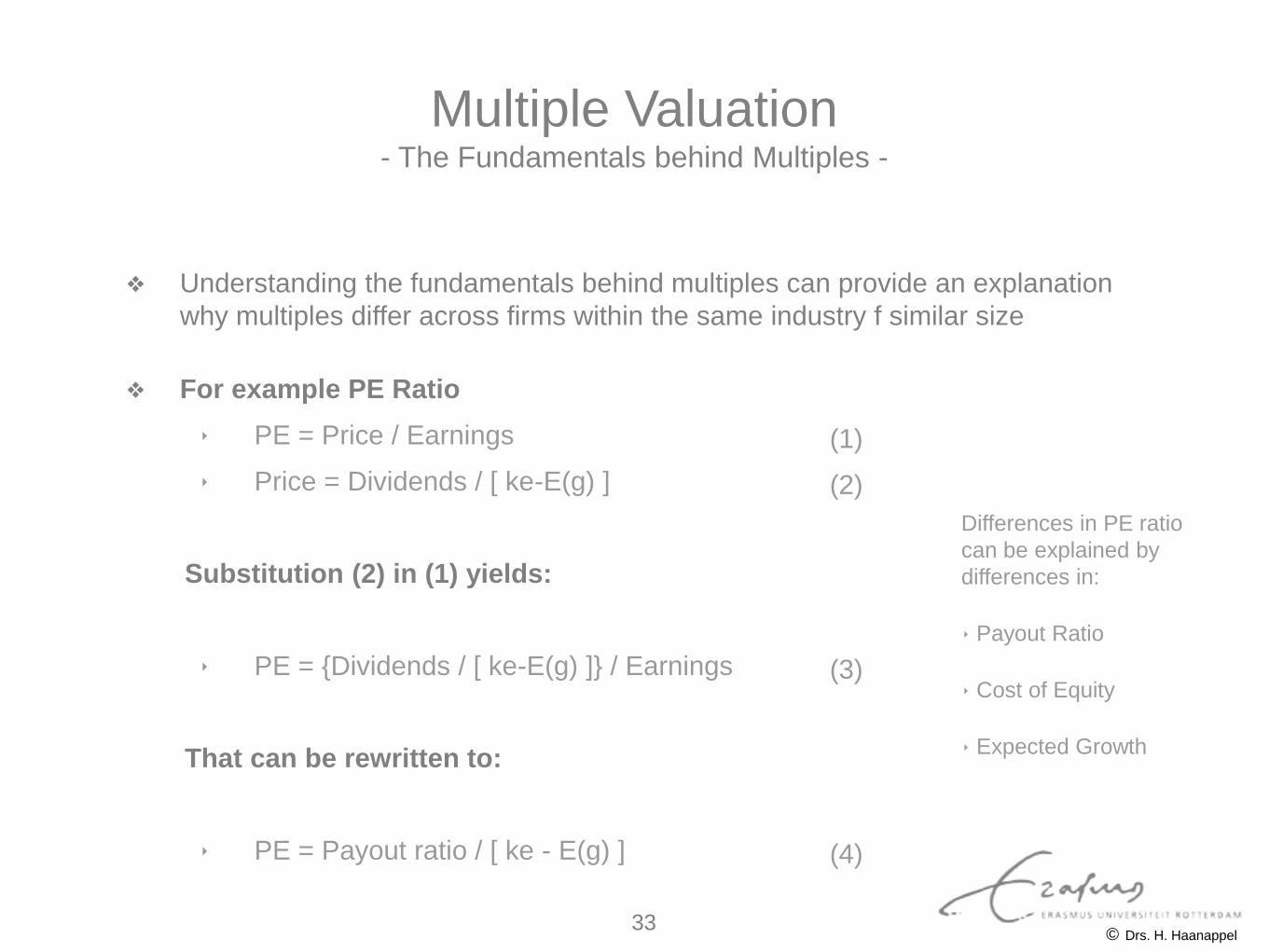
❖ For example PE Ratio
‣ PE = Price / Earnings
‣ Price = Dividends / [ ke-E(g) ]
Substitution (2) in (1) yields:
‣ PE = {Dividends / [ ke-E(g) ]} / Earnings
That can be rewritten to:
‣ PE = Payout ratio / [ ke - E(g) ]
❖ Understanding the fundamentals behind multiples can provide an explanation
why multiples differ across firms within the same industry f similar size
(1)
(2)
(3)
(4)
Differences in PE ratio
can be explained by
differences in:
‣ Payout Ratio
‣ Cost of Equity
‣ Expected Growth
Multiple Valuation - The Fundamentals behind Multiples -
© Drs. H. Haanappel 33
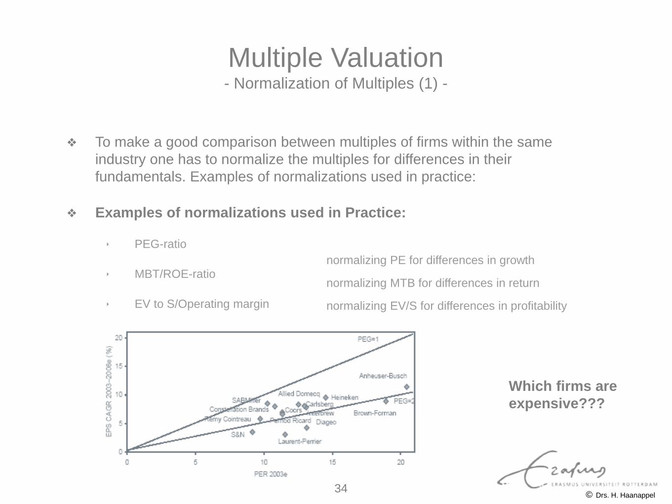
❖ Examples of normalizations used in Practice:
‣ PEG-ratio
‣ MBT/ROE-ratio
‣ EV to S/Operating margin
❖ To make a good comparison between multiples of firms within the same
industry one has to normalize the multiples for differences in their
fundamentals. Examples of normalizations used in practice:
Which firms are
expensive???
normalizing PE for differences in growth
normalizing MTB for differences in return
normalizing EV/S for differences in profitability
Multiple Valuation - Normalization of Multiples (1) -
© Drs. H. Haanappel 34
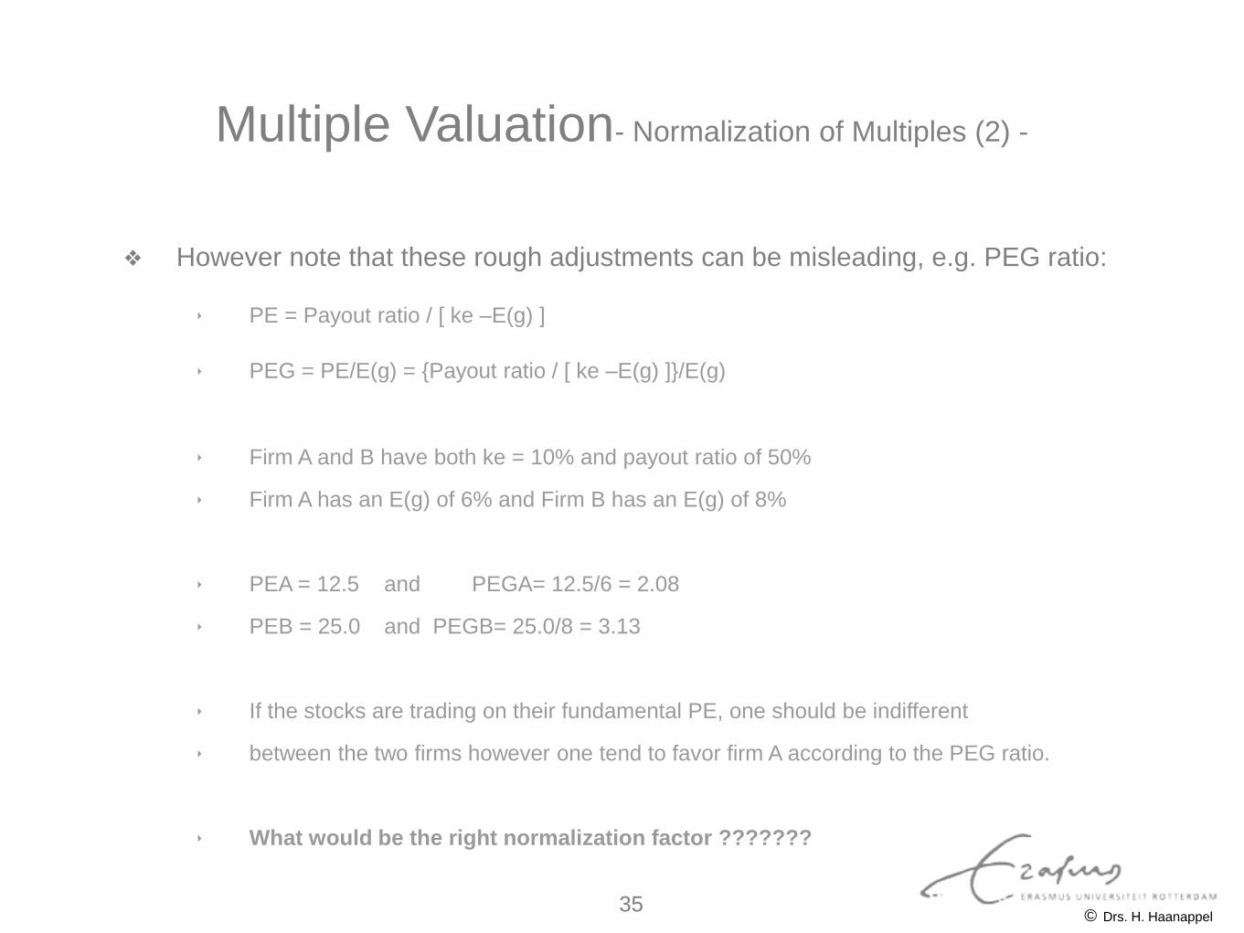
❖ However note that these rough adjustments can be misleading, e.g. PEG ratio:
‣ PE = Payout ratio / [ ke –E(g) ]
‣ PEG = PE/E(g) = {Payout ratio / [ ke –E(g) ]}/E(g)
‣ Firm A and B have both ke = 10% and payout ratio of 50%
‣ Firm A has an E(g) of 6% and Firm B has an E(g) of 8%
‣ PEA = 12.5 and PEGA= 12.5/6 = 2.08
‣ PEB = 25.0 and PEGB= 25.0/8 = 3.13
‣ If the stocks are trading on their fundamental PE, one should be indifferent
‣ between the two firms however one tend to favor firm A according to the PEG ratio.
‣ What would be the right normalization factor ???????
Multiple Valuation- Normalization of Multiples (2) -
© Drs. H. Haanappel 35
Multiple Valuation - Regression Analysis on Multiples -
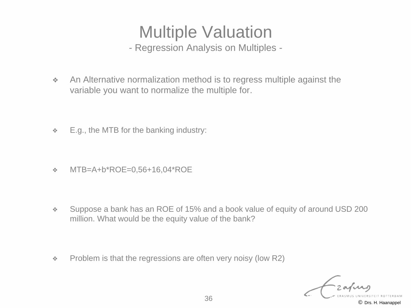
❖ An Alternative normalization method is to regress multiple against the
variable you want to normalize the multiple for.
❖ E.g., the MTB for the banking industry:
❖ MTB=A+b*ROE=0,56+16,04*ROE
❖ Suppose a bank has an ROE of 15% and a book value of equity of around USD 200
million. What would be the equity value of the bank?
❖ Problem is that the regressions are often very noisy (low R2)
© Drs. H. Haanappel 36
© Prof. dr. J.T.J. Smit
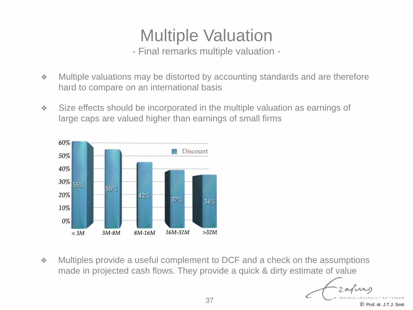
❖ Multiple valuations may be distorted by accounting standards and are therefore
hard to compare on an international basis
❖ Size effects should be incorporated in the multiple valuation as earnings of
large caps are valued higher than earnings of small firms
❖ Multiples provide a useful complement to DCF and a check on the assumptions
made in projected cash flows. They provide a quick & dirty estimate of value
Multiple Valuation - Final remarks multiple valuation -
37
Concluding Remarks
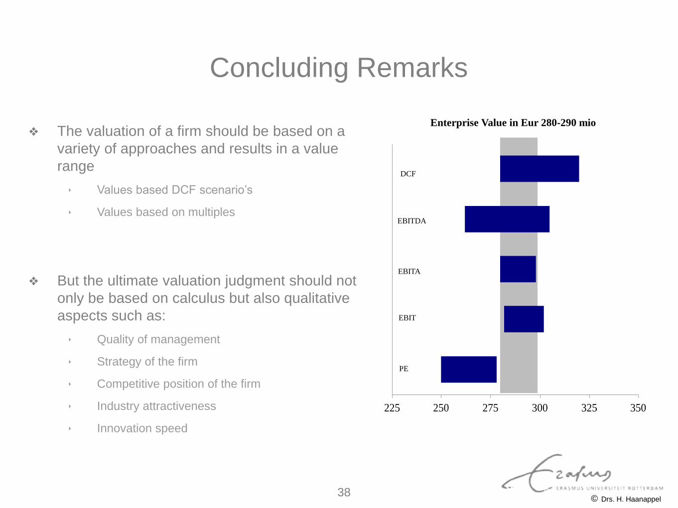
❖ The valuation of a firm should be based on a
variety of approaches and results in a value
range
‣ Values based DCF scenario’s
‣ Values based on multiples
❖ But the ultimate valuation judgment should not
only be based on calculus but also qualitative
aspects such as:
‣ Quality of management
‣ Strategy of the firm
‣ Competitive position of the firm
‣ Industry attractiveness
‣ Innovation speed
225 250 275 300 325 350
DCF
EBITDA
EBITA
EBIT
PE
Enterprise Value in Eur 280-290 mio
© Drs. H. Haanappel 38