Embed Size (px)
Citation preview
ISTANBUL TECHNICAL UNIVERSITY GRADUATE SCHOOL OF SCIENCE ENGINEERING AND TECHNOLOGY
M.Sc. THESIS
AUGUST 2014
FINITE ELEMENT ANALYSIS, OPTIMUM DESIGN AND COST-EFFECTIVE MANUFACTURING OF ADVANCED COMPOSITE GRID-STIFFENED
STRUCTURES FOR AIRCRAFT FUSELAGE APPLICATIONS
Onur COŞKUN
Department of Aeronautics and Astronautics Engineering
Aeronautics and Astronautics Engineering Programme

AUGUST 2014
ISTANBUL TECHNICAL UNIVERSITY GRADUATE SCHOOL OF SCIENCE ENGINEERING AND TECHNOLOGY
FINITE ELEMENT ANALYSIS, OPTIMUM DESIGN AND COST-EFFECTIVE MANUFACTURING OF ADVANCED COMPOSITE GRID-STIFFENED
STRUCTURES FOR AIRCRAFT FUSELAGE APPLICATIONS
M.Sc. THESIS
Onur COŞKUN (511111131)
Department of Aeronautics and Astronautics Engineering
Aeronautics and Astronautics Engineering Programme
Thesis Advisor: Prof. Dr. Halit S. TÜRKMEN

AĞUSTOS 2014
İSTANBUL TEKNİK ÜNİVERSİTESİ FEN BİLİMLERİ ENSTİTÜSÜ
GRİD TAKVİYELİ İLERİ KOMPOZİT YAPILARIN UÇAK GÖVDESİ İÇİN SONLU ELEMANLAR ANALİZİ, OPTİMUM TASARIMI VE UYGUN
MALİYETLİ ÜRETİMİ
YÜKSEK LİSANS TEZİ
Onur COŞKUN (511111131)
Uçak ve Uzay Mühendisliği Anabilim Dalı
Uçak ve Uzay Mühendisliği (DAP)
Tez Danışmanı: Prof. Dr. Halit S. Türkmen

Thesis Advisor : Prof. Dr. Halit S. Türkmen .............................. İstanbul Technical University
Jury Members : Assoc. Prof. Dr. Vedat Ziya Doğan ............................. İstanbul Technical University
Assoc. Prof. Dr. Zafer Kazancı .............................. Turkish Air Force Academy
Onur COŞKUN, a M.Sc. student of ITU Institute of Science and Technology student ID 511111131, successfully defended the thesis entitled FINITE ELEMENT ANALYSIS, OPTIMUM DESIGN AND COST-EFFECTIVE MANUFACTURING OF ADVANCED COMPOSITE GRID-STIFFENED STRUCTURES FOR AIRCRAFT FUSELAGE APPLICATIONS”, which he prepared after fulfilling the requirements specified in the associated legislations, before the jury whose signatures are below.
Date of Submission : 05 May 2014 Date of Defense : 25 August 2014
v

vi

To my dear family,
vii

viii
FOREWORD
I would like to sincerely thank and appreciate to my supervising professor, Dr. Christos Kassapoglou for his guidance, support, and encouragement throughout my research in every aspect. My gratitude goes to the committee members: Sonell Shroff and Dr. Halit S. Türkmen, for providing guidance and support. Most of all, thanks to my family and Fatma Nur Evren, for their love, support, and encouragement. Without their love and support, none of this research work would have proceeded. Finally, I would like to thank everyone from TU DELFT Composite Lab who have helped me with my research. August 2014
Onur COŞKUN (Aeronautical Engineer)
ix

x
TABLE OF CONTENTS
Page FOREWORD ............................................................................................................. ix TABLE OF CONTENTS ......................................................................................... xi ABBREVIATIONS ................................................................................................. xiii LIST OF TABLES ................................................................................................... xv LIST OF FIGURES ............................................................................................... xvii SUMMARY ............................................................................................................. xix ÖZET ....................................................................................................................... xxi 1. INTRODUCTION .................................................................................................. 1
1.1 Background ........................................................................................................ 1 1.2 Objectives and Approach to the Thesis .............................................................. 4 1.3 Scope .................................................................................................................. 5
2. LITERATURE REVIEW ..................................................................................... 7 2.1 Analytical Approaches to Grid Stiffened Panels ............................................... 7 2.2 Finite Element Approaches to Grid Stiffened Panels ........................................ 8 2.3 Methods of Grid Stiffened Panel Manufacture ................................................ 11 2.4 Optimization of Grid Stiffened Panels ............................................................. 15
3. THEORETICAL MODEL AND FUNDAMENTAL EQUATIONS .............. 17 3.1 Classical Laminate Theory ............................................................................... 17
3.1.1 Material property of intersecting nodes .................................................... 23 3.2 Material Failure Analysis ................................................................................. 25 3.3 Instability of Stiffeners ..................................................................................... 27
3.3.1 Rib crippling ............................................................................................. 27 3.3.2 Column buckling ....................................................................................... 28
4. FINITE ELEMENT ANALYSIS OF FUSELAGE .......................................... 29 4.1 Modeling .......................................................................................................... 29 4.2 Boundary Conditions and Loading .................................................................. 31 4.3 Comparison ...................................................................................................... 33
5. FINITE ELEMENT ANALYSIS OF THE COMPOSITE AGS PANEL ...... 37 5.1 Modeling .......................................................................................................... 37 5.2 Meshing ............................................................................................................ 38
5.2.1 Quad elements ........................................................................................... 39 5.2.2 Quad and tria elements .............................................................................. 40
5.3 Boundary Conditions and Loading .................................................................. 40 5.3.1 Load case 1 ................................................................................................ 40 5.3.2 Load case 2 ................................................................................................ 41 5.3.3 Load case 3 ................................................................................................ 41 5.3.4 Local 3D case ............................................................................................ 42
5.4 Solutions ........................................................................................................... 43 5.4.1 Linear static ............................................................................................... 43 5.4.2 Buckling .................................................................................................... 44
5.5 Analyses Results .............................................................................................. 46 5.5.1 Displacement of the composite AGS plate ............................................... 46 5.5.2 Stress distribution along stiffeners ............................................................ 47
xi
5.5.3 Stress distribution on the skin ................................................................... 49 5.5.4 Inter-laminar stresses on 3D model ........................................................... 50 5.5.5 Buckling modes of ags panel .................................................................... 51
6. FINITE ELEMENT OPTIMISATION OF AGS PANEL ............................... 55 6.1 Msc Nastran Optimization – How it works? .................................................... 55 6.2 MSC. Patran PCL functions ............................................................................. 57 6.3 Design Model ................................................................................................... 58 6.4 Optimization Results ........................................................................................ 60
7. FABRICATION OF ADVANCED GRID STIFFENED (AGS) COMPOSITE STRUCTURE ........................................................................................................... 63
7.1 Material System ................................................................................................ 63 7.2 Tooling System ................................................................................................ 64
7.2.1 Aluminum block tooling ........................................................................... 64 7.2.2 Expansion block tooling ............................................................................ 65
7.3 Manufacturing Steps for Composite AGS Panel .............................................. 66 7.3.1 First trial of composite ags panel manufacturing ...................................... 66 7.3.2 Second trial of composite ags panel manufacturing (1*1 cell) ................. 67
7.4 2*2 cell Composite AGS Panel Manufacturing ............................................... 70 8. CONCLUSIONS AND RECOMMENDATIONS ............................................. 73
8.1 Conclusions ...................................................................................................... 73 8.2 Recommendations ............................................................................................ 74
REFERENCES ......................................................................................................... 77 APPENDICES .......................................................................................................... 81 APPENDIX A ........................................................................................................... 82 APPENDIX B ........................................................................................................... 85 CURRICULUM VITAE .......................................................................................... 87
xii

ABBREVIATIONS
AFRL : Air Force Research Laboratory AGS : Advanced Grid Stiffened Structure CNC : Computer Numerical Control CFRP : Carbon Fiber Reinforced Plastic CTE : Coefficient Of Thermal Expansion DOF : Degree of Freedom ESM : Equivalent stiffness method FE : Finite Element FEA : Finite Element Analysis FEM : Finite Element Method IUPAC : International Union of Pure and Applied Chemistry LC : Load Case NASA : National Aeronautics and Space Administration PEG : Pin Enhanced Geometry PCL : The PATRAN Command Language RTM : Resin Transfer Molding TRIG : Tooling-Reinforced Interlaced Grid UD : Unidirectional
xiii

xiv
LIST OF TABLES
Page
Table 3.1 : Material property of intersecting nodes. ................................................. 24 Table 3.2 : Material property of transition regions near intersecting nodes. ............ 25 Table 3.3 : Failure strength of intersecting nodes. .................................................... 27 Table 4.1 : Comparison of shell forces. .................................................................... 35 Table 6.1 : Optimization results for various models. ................................................ 62
xv

xvi
LIST OF FIGURES
Page
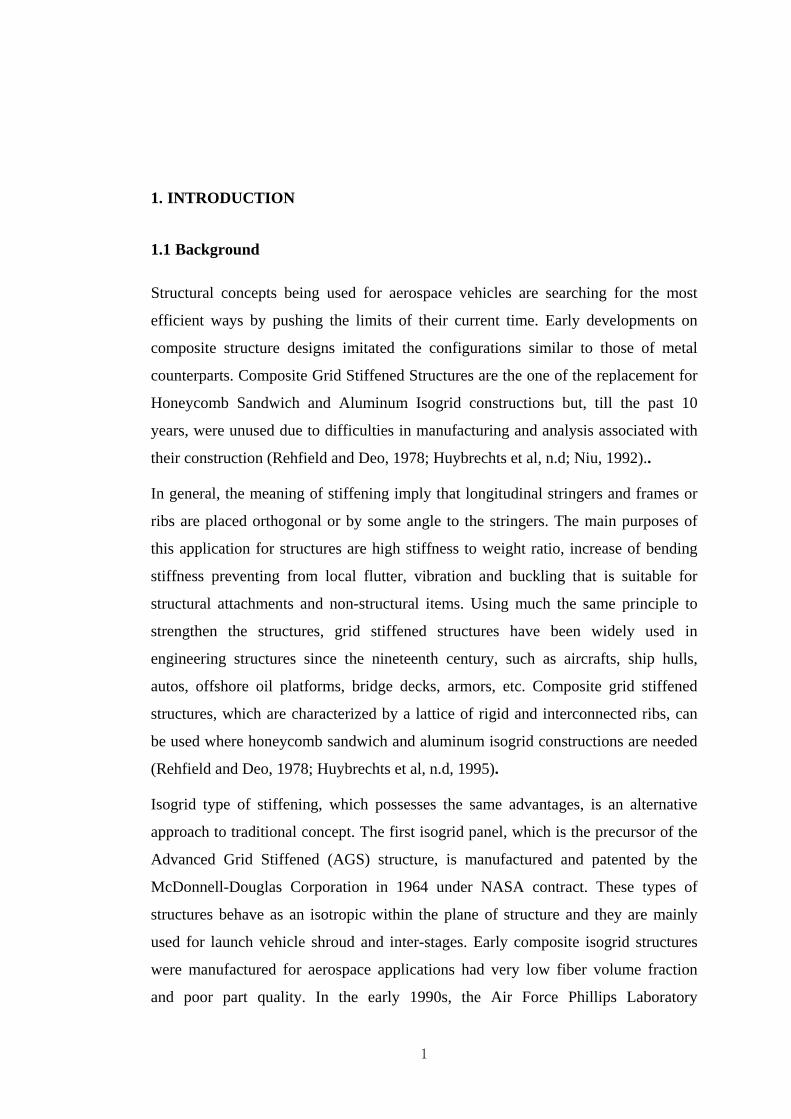
Figure 1.1 : Types of grid-stiffened panels. ................................................................ 2 Figure 4.1 : Fuselage FE model and cross section. ................................................... 30 Figure 4.2 : Quasi-isotropic laminate sequences for skin. ........................................ 31 Figure 4.3 : Symmetry boundary conditions for fuselage. ........................................ 32 Figure 4.4 : Comparison of displacement sum. ........................................................ 33 Figure 4.5 : Comparison of circumferential shell forces. ......................................... 34 Figure 5.1 : The Composite AGS panel is modeled with CQUAD4. ....................... 39 Figure 5.2 : The Composite AGS panel is modeled with CQUAD4 and CTRIA3. . 40 Figure 5.3 : The Composite AGS panel LC1 BC and loading. ................................. 41 Figure 5.4 : The Composite AGS panel LC2 BC and loading. ................................. 42 Figure 5.5 : The Composite AGS panel Local 3D BC and 2D nodal displacement
application regions. ............................................................................. 43 Figure 5.6 : Displacement sums of the Composite AGS Plate for different load
cases. .................................................................................................... 46 Figure 5.7 : Maximum ply stresses (MPa) along 35° direction (Load Case 2). ....... 47 Figure 5.8 : Maximum ply stresses (MPa) along -35° direction (Load Case 2). ...... 48 Figure 5.9 : Maximum ply stresses (MPa) along 0° direction (Load Case 2). ......... 48 Figure 5.10 : Maximum ply stresses (MPa) along 90° direction (Load Case 2).. .... 49 Figure 5.11 : Maximum ply stresses (MPa) along 0°, 90° and 45° direction (Load
Case 2). ................................................................................................ 49 Figure 5.12 : Ply stresses (MPa) 35° direction (Load Case 2) and interlaminar
normal stress. ....................................................................................... 51 Figure 5.13 : Inter-laminar shear stresses (MPA) (Load Case 2). ............................ 51 Figure 5.14 : Buckling modes and eigenvalues for Load Case 2. ............................. 52 Figure 6.1 : Rib design parameters at the beginning of the design cycle. ................ 59 Figure 6.2 : Skin lay-up for design model of composite AGS panel. ....................... 59 Figure 7.1 : Female and male Aluminum molds. ...................................................... 65 Figure 7.2 : Silicon rubber molds - One cell and 2*2 cells. ...................................... 65 Figure 7.3 : Dry/Hand lay-up fiber bundles using carbon fiber rolls. ....................... 66 Figure 7.4 : Removal of aluminum mold and silicon block placement. ................... 67 Figure 7.5 : Dry/Hand lay-up fiber bundles using carbon fiber rolls. ....................... 68 Figure 7.6 : Semi-permeable membrane and peel ply placement. ............................ 68 Figure 7.7 : Vacuum assisted resin infusion system for composite AGS panel. ...... 69 Figure 7.8: Vacuum assisted resin infusion system and cured composite AGS panel.
............................................................................................................. 70 Figure 7.9 : Dry/hand lay-up winding process and metal frames placed at the ends of
mold. .................................................................................................... 71 Figure 7.10 : Dry/hand lay-up winding process and cured composite AGS panel. .. 72 Figure A.1 : Maximum ply stresses (MPa) for Load Case 1 on ribs: (a)0° direction.
(b) 35° direction. (c) -35° direction. (d) 90° direction. ....................... 80
xvii

Figure A.2 : Maximum ply stresses (MPa) for Load Case 3: (a)0° direction. (b) 35° direction. (c) -35° direction. (d) 90° direction. .................................... 81
Figure A.3 : MSC. Patran composite material definitions ........................................ 83
xviii
FINITE ELEMENT ANALYSIS, OPTIMUM DESIGN AND COST-EFFECTIVE MANUFACTURING OF ADVANCED COMPOSITE GRID-
STIFFENED STRUCTURES FOR AIRCRAFT FUSELAGE APPLICATIONS
SUMMARY
Structural concepts being used for aerospace vehicles are searching for the most efficient ways by pushing the limits of their current time. In general, the meaning of stiffening imply that longitudinal stringers and frames or ribs are placed orthogonal or by some angle to the stringers. The main purposes of this application for structures are high stiffness to weight ratio, increase of bending stiffness preventing from local flutter, vibration and buckling, suitable for structural attachments and non-structural items.
Advanced Grid Stiffened (AGS) structures possesses wide variety of possibilities to design and manufacture stiffeners with different spacing, nodal offset, stiffener angle, number of stiffener, thickness of the skin, etc. AGS structures, which have complex component geometries, require the use of finite element analysis techniques for detailed structural analysis. Analytical methods cannot predict the local stress distributions and local failure types. Failure types of composite AGS structures under in-plane loads and under the effect of out of plane shear loads are categorized as five dominant failure modes. These are; instability of total panel, which is referred to as global buckling, local skin buckling, local buckling or crippling of the stiffeners, material failure and delamination caused by inter-laminar shear stresses. Understanding the failure behavior and stress distributions on the composite AGS panel under inplane loading and the effect of out of plane shear loads is important to structural design. Thus, all five different failure modes and stresses at critical locations like nodes of AGS panel are considered in the design and need to be considered in validation and certification phases.
AGS panel is modeled and analyzed using 2D quadrilateral elements using MSC Patran/MSC Nastran. Stress distributions along the stiffeners and the skin can be separately taken from their element centroids and different buckling modes of the AGS panel can be observed using SOL105. MSC Patran PCL functions are used to change the stiffener spacing. An optimization cycle is set-up using MSC Nastran SOL200 solver, which takes into account stiffener crippling and material failure as design constraints. The inter-laminar shear stresses along the height of the stiffener and at the skin-stiffener interface section is taken from local 3D model of highly stressed regions.
The decision is made for the optimized panel under mixed loading, which is shear-bi-axial compression respectively 175 N/mm and 60 N/mm -150N/mm. According to optimization results, stiffener height is 21.377 mm, stiffener spacing is 205.8 mm.
xix

The manufacturing of the AGS panel, which is laborious with any technique done in previous studies, is accomplished successfully by using Vacuum Assisted Resin Transfer Molding like technique. The integral manufacturing of grids and skin using resin infusion provides low-cost manufacturing of AGS panels. In this process, pattern of the grids are printed using 3D printers and silicon rubber, which takes the shape of printings, which are used to make mold, then fibers are laid into the grooves. After laying all the fibers, which can reach 50% percent fiber fraction just by hand process, skin is put on the side where fibers are ending. After resin infusion, composite AGS panel is cured at elevated temperature in the oven.
xx
GRID TAKVİYELİ İLERİ KOMPOZİT YAPILARIN UÇAK GÖVDESİ İÇİN SONLU ELEMANLAR ANALİZİ, OPTİMUM TASARIMI VE UYGUN
MALİYETLİ ÜRETİMİ
ÖZET
Uçak ve uzay yapıları için geliştirilen ve içinde bulunduğumuz zaman dilimine ile paralel teknolojik gelişmeler ile uygulanabilen üretim yöntemleri her geçen gün daha da ilerlemektedir. Bu ilerleyişin ve artan araştırmaların doğal bir sonucu olarak kompozit malzemeler ve bunlardan oluşturulan yapılar metal, alüminyum gibi malzemelerin yerini almaktadır. Grid Takviyeli İleri Kompozit yapılar ise bu malzemelerle geliştirilmiş farklı tasarım ve üretim yöntemleri le ortaya çıkmıştır. Genel anlamı ile grid takviye, boyuna kirişler halinde ortogonal veya çeşitli açılarla yerleştirilmiş yapılara denmektedir. Yapılarda bu tür bir kompozit yapının kullanılmasının başlıca nedenleri yüksek sertlik-ağırlık oranı olması, eğilme rijitliğini artırarak bölgesel fluter, titreşim ve burkulmayı önlemesi, yapısal eklemelere ve yapısal olmayan öğelere uygun olması.
Grid Takviyeli İleri Kompozit yapılar tasarım ve üretim açısından birçok çeşitliliğe olanak vermektedir. Bu çeşitlilik kirişlerin açıklığı, düğüm noktası kaçıklığı, kiriş açısı, kiriş sayısı, yüzey plakasının kalınlığı, vs. ile sağlanabilmektedir. Bu tip karmaşık değişkenlere sahip olan bu sistem şu an için analitik olarak tam çözülememektedir. Bu nedenle sonlu elemanlar analiz yöntemleri ile modellenip detaylı bir analize ihtiyaç duyulmaktadır. Bu ihtiyacın da ana nedeni lokal gerilme dağılımlarının ve lokal kırılma ve kopmaların incelenebilmesidir.
Grid Takviyeli İleri Kompozit yapılar çeşitli kırılma tiplerine sahiptir. Bunlar, düzlem içi yükler ve düzlem dışı kayma gerilmelerine bağlı olarak beşe ayrılabilirler; tüm panelin kararsızlığına yol açan burkulma davranışı, lokal yüzey burkulması, lokal kiriş burkulması, malzeme kopması ve tabakalar arası kayma gerilmesinden kaynaklanan tabakalar arası kayma davranışıdır. Yapısal tasarım açısından kırılma davranışının ve gerilme dağılımlarının Grıd Takviyeli İleri Kompozit malzemeler için bilinmesi önemli bir parametredir. Bu önemin nedeni, kritik noktalardaki beş farklı kırılma mekanizması tasarımda olduğu kadar aynı zamanda onaylama ve sertifikasyon süreçleri içinde göz önünde bulundurulması gerekliliğidir.
Grid Takviyeli İleri Kompozit yapı 2 boyutlu sonlu elamanlar yöntemi kullanılarak dörtgen elemanlar kullanılarak modellenmiştir. Bu elemanlar MSC Patran/Msc Nastran adlı ticari program içerisinde tanımlanmış olan eleman tipleri kullanılarak yapılmıştır. Yapılan modellemede klasik yöntemlerin aksine kirişlerin olduğu yerlerde çift eleman kullanılmış ve bu şekilde gerekli olan katılık 2 boyutlu olarak tanımlanabilmiştir. Bu tasarım tüm boyutlandırmalar tanımlandıktan sonra yapılabilmektedir, başka bir deyişle sadece kiriş ve yüzey kalınlığı program içinden girilen değerler ile değiştirilebilmektedir. Bunun haricinde yapılması gereken boyut değişimleri MSC. Patran PCL fonksiyonları kullanılarak yapılmıştır.
xxi
MSC. Patran PCL fonksiyonun en önemli işlevi makro gibi çalışabilmesi ve bu sayede her defasında belirli değerlere kadar olan kiriş açıklığı değişimleri için sonlu elemanlar örgüsünü Mathematica’da yazılan kod sayesinde yeniden yaratabilmesidir.
Grid Takviyeli İleri Kompozit yapı için 3 boyutlu sonlu elamanlar yöntemi kullanılarak da modellenmiştir. Bu modelleme ile tabakalar arası kayma gerilmesinden kaynaklanan tabakalar arası kayma davranışı olup olmadığı karbon fiber destekli plakalarda 50 MPa gerilme değeri ile karşılaştırılıp karar verilmektedir. Bu yöntemdeki sınır koşulları 2 boyutlu modelde kritik olduğuna kara verilen bölgeler için eşdeğer eleman genişliğinde yapılan 3 boyutlu modele 2 boyutlu analiz sonuçlarından gelen öteleme ve dönme hareketinin uygun düğüm noktalarına uygulanması ile tanımlamıştır.
Grid Takviyeli İleri Kompozit yapı için 2 boyutlu sonlu elamanlar yöntemi kullanılarak gerilme ve burkulma analizleri yapılmıştır. Bu analizler için için Nastran SOL101 ve SOL105 kütüphaneleri kullanılmıştır. Yapılan modelleme tekniğiyle birlikte kirişlerin ana yük taşıyan fiber doğrultusu boyunca gerilme değimleri gözlenebilmiş ve tasarım hakkında genel bir gözlem yapılabilmiştir. Yüzey üzerindeki gerilme değimleri ile ona bağlı olan kirişlerdeki gerilmeler karşılaştırılmış ve mantıklı bir fizik davranışı elde edilmiştir. Burkulma analizlerinde ise yapı farklı yükleme koşullarında incelenip, nihayetinde en kritik olan yükleme koşulu için 10 farklı burkulma modu incelenmiştir. Bu inceleme sonucunda gerçekleşen burkulmaların sadece lokal yüzey hücre burkulmaları olduğu gözlemlenmiştir. Nastran’ın hesapladığı özdeğer vektörü 1. mod için 1 değerine yaklaşıktır. Bu da demek oluyor ki bu yükleme koşulu 2 için ilk mod aynı zamanda kırılma gerilmesinin de oluştuğu yük durumuna karşılık gelmektedir.
Grid Takviyeli İleri Kompozit yapı için 2 boyutlu sonlu elamanlar yöntemi kullanılarak optimizasyon analizleri de yapılmıştır. Bu analiz için Nastran SOL200 kütüphanesi kullanılmıştır. Tasarım kısıtları olarak malzeme kırılması, lokal kiriş burkulması ve Euler burkulması referans olarak alınmıştır. Yapılan optimizasyon çalışması Nastran’ın kendi içerisindeki algoritmaları kullanması ile gerçekleştirmiştir. Burada “hard convergence” denilen bir yakınsama metodu ile denklemler iterasyonlarla çözülmektedir. Her döngüde elde edilen yakınsaklık değerleri ile tüm sonlu elemanlar modeli yeniden çözülmekte ve en son iterasyona kadar bu süreç devam etmektedir. Yapılan bu çalışma sonucunda, verilen yükleme altında 2 boyutlu gerilme analizi için kullanılan model kullanılmış olup, optimum boyutlar elde edilmiş ve bunların yukarıda anlatıldığı gibi ayrıntılı analizleri yapılmıştır.
Grid Takviyeli İleri Kompozit yapı için üretim yöntemi de geliştirilmiş olup başarılı bir şekilde uygulanmıştır. Bu üretim yöntemi daha çok literatür üzerinden yapılan çalışmalar üzerinden yola çıkılarak geliştirilmiştir. Vakum destekli reçine infüzyonu ile yapılan üretim silikon kalıplar içerisinde gerçekleştirilmiştir. Kullanılan silikon kalıplar belirli noktalarından delikler açılarak reçine ile beslenmiştir. Açılan bu delikler direkt olarak kirişlerin yatırıldığı boşlukların olduğu kısımlara açılmıştır. Gösterge basını 55 mbar olarak ayarlanıp reçinenin kurulan düzenek içinde ilerlemesi sağlanmıştır. Yüzeyde ve kirişlerin içinde ilerleyen reçine kalıbın bittiği noktalarda dışarı çıkmaması için yarı geçirgen bir zar ile örtülmüştür. Bu zar hava akışını sağlamakla beraber reçine gibi sıvı bir maddenin geçişine izin vermemekte ve bu şekilde reçine içerde kalmakta ve bütün fiberler boyunca bir dağılım gösterip en kolay bulduğu yoldan dışarı kaçamamaktadır.
xxii

İnfüzyon işlemi yapıldıktan sonra malzeme düzeneği aynı vakum altında fırınlanmakta ve 5 saat sonra çıkartılıp silikon kalıptan çıkarılmaktadır. Bu yöntem ilk olarak tek hücre yapısı için denenmiş olur daha sonra 2*2 hücre için denenmiş ve elle yatırma işlemi nedeniyle daha fazla hücre sayısı için otomasyon yöntemlerin kullanılmasına karar verilmiştir. Bu başarılı üretim sonuçlarından sonra yapı makro boyutlarda çekim yapan bir kamera ile incelenmiş ve kuru veya fiber çekme kuvvetinin kaybı ile oluşmuş üretimden gelen hatalar tespit edilmiştir. Ayrıca reçinenin düğüm noktalarında fiber hacminin artması sonucu nasıl dağıldığı gözlemlenmiş ve literatür üzerindeki çalışmalarla kıyaslanmıştır.
xxiii

xxiv
1. INTRODUCTION
1.1 Background
Structural concepts being used for aerospace vehicles are searching for the most
efficient ways by pushing the limits of their current time. Early developments on
composite structure designs imitated the configurations similar to those of metal
counterparts. Composite Grid Stiffened Structures are the one of the replacement for
Honeycomb Sandwich and Aluminum Isogrid constructions but, till the past 10
years, were unused due to difficulties in manufacturing and analysis associated with
their construction (Rehfield and Deo, 1978; Huybrechts et al, n.d; Niu, 1992)..
In general, the meaning of stiffening imply that longitudinal stringers and frames or
ribs are placed orthogonal or by some angle to the stringers. The main purposes of
this application for structures are high stiffness to weight ratio, increase of bending
stiffness preventing from local flutter, vibration and buckling that is suitable for
structural attachments and non-structural items. Using much the same principle to
strengthen the structures, grid stiffened structures have been widely used in
engineering structures since the nineteenth century, such as aircrafts, ship hulls,
autos, offshore oil platforms, bridge decks, armors, etc. Composite grid stiffened
structures, which are characterized by a lattice of rigid and interconnected ribs, can
be used where honeycomb sandwich and aluminum isogrid constructions are needed
(Rehfield and Deo, 1978; Huybrechts et al, n.d, 1995).
Isogrid type of stiffening, which possesses the same advantages, is an alternative
approach to traditional concept. The first isogrid panel, which is the precursor of the
Advanced Grid Stiffened (AGS) structure, is manufactured and patented by the
McDonnell-Douglas Corporation in 1964 under NASA contract. These types of
structures behave as an isotropic within the plane of structure and they are mainly
used for launch vehicle shroud and inter-stages. Early composite isogrid structures
were manufactured for aerospace applications had very low fiber volume fraction
and poor part quality. In the early 1990s, the Air Force Phillips Laboratory
1
manufactured isogrid structure using tooling made of silicon rubber and achieved
high quality and high strength-weight ratios .
The interest for composite grid stiffened structures was decreasing for many decades
due to complex manufacturing and analysis technique needed for application. In
recent years, the Boeing Company, the US Air Force Research Lab, McDonnell-
Douglas, Alliant Tech Systems, Stanford University, and others have made some
researches and publications with the aid of developing technology on computation
and manufacturing. They are now currently being investigated by several aerospace
structure manufacturers (Rehfield and Deo, 1978; Huybrechts et al, n.d).
Isogrid pattern, which consists of equilateral pattern, has been optimized and
changed its shape for specific loading situations in past few years. With the new
applications, the prefix “iso” is replaced by Advanced Grid Stiffened (AGS)
structure patterns. The source of increasing interest on composite materials for the
grid stiffened panel is the high directionality of composite materials. The high
directionality allows material’s stiffness to be directed along the critical direction and
a substantial increase in the stiffener strength along rib length (Huybrechts and Tsai,
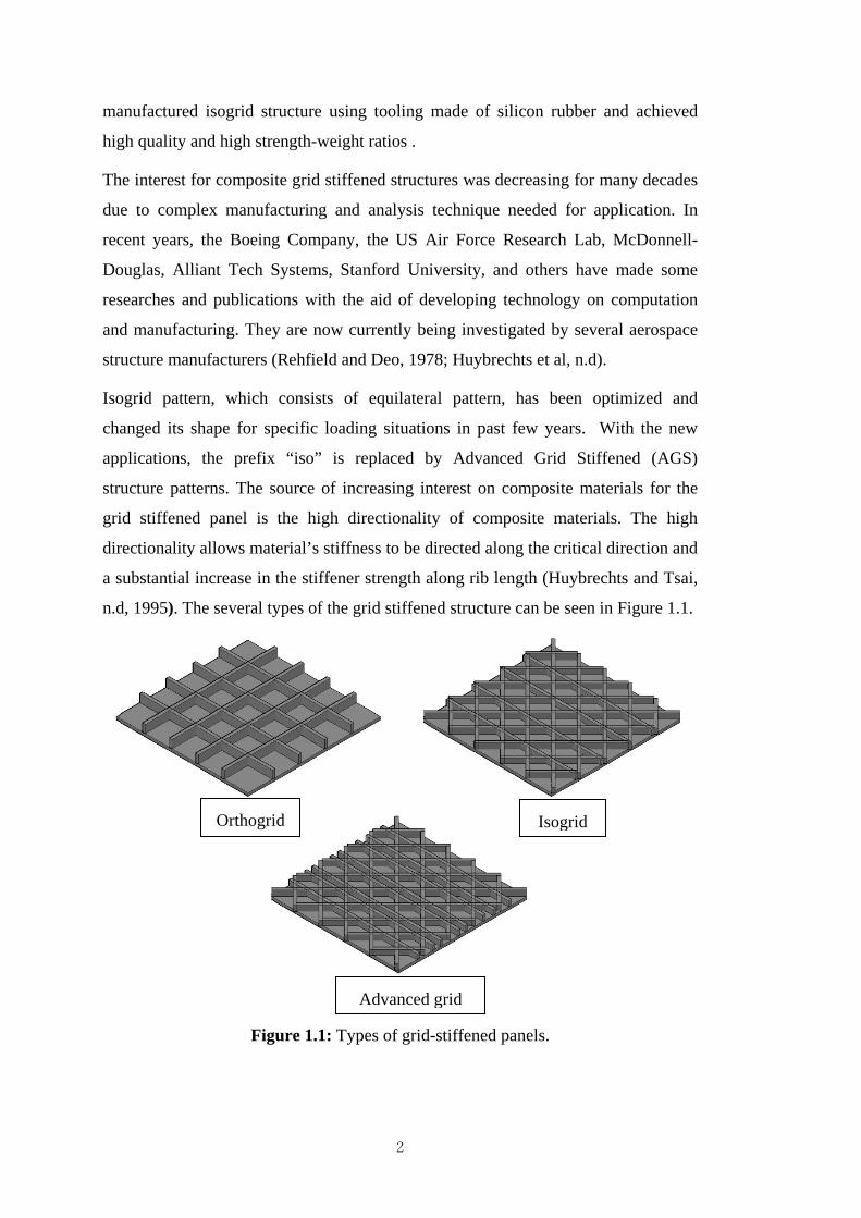
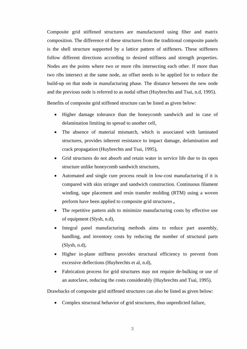
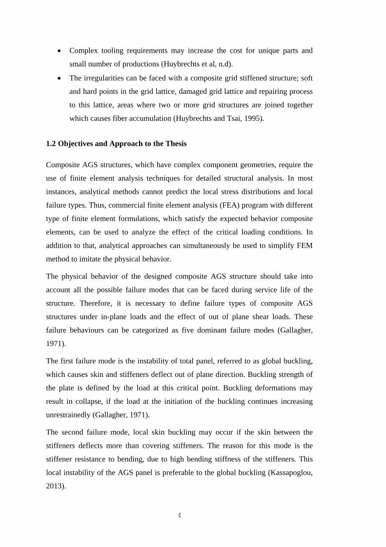
n.d, 1995). The several types of the grid stiffened structure can be seen in Figure 1.1.
Figure 1.1: Types of grid-stiffened panels.
Orthogrid Isogrid
Advanced grid
2
Composite grid stiffened structures are manufactured using fiber and matrix
composition. The difference of these structures from the traditional composite panels
is the shell structure supported by a lattice pattern of stiffeners. These stiffeners
follow different directions according to desired stiffness and strength properties.
Nodes are the points where two or more ribs intersecting each other. If more than
two ribs intersect at the same node, an offset needs to be applied for to reduce the
build-up on that node in manufacturing phase. The distance between the new node
and the previous node is referred to as nodal offset (Huybrechts and Tsai, n.d, 1995).
Benefits of composite grid stiffened structure can be listed as given below:
• Higher damage tolerance than the honeycomb sandwich and in case of
delamination limiting its spread to another cell,
• The absence of material mismatch, which is associated with laminated
structures, provides inherent resistance to impact damage, delamination and
crack propagation (Huybrechts and Tsai, 1995),
• Grid structures do not absorb and retain water in service life due to its open
structure unlike honeycomb sandwich structures,
• Automated and single cure process result in low-cost manufacturing if it is
compared with skin stringer and sandwich construction. Continuous filament
winding, tape placement and resin transfer molding (RTM) using a woven
preform have been applied to composite grid structures ,
• The repetitive pattern aids to minimize manufacturing costs by effective use
of equipment (Slysh, n.d),
• Integral panel manufacturing methods aims to reduce part assembly,
handling, and inventory costs by reducing the number of structural parts
(Slysh, n.d),
• Higher in-plane stiffness provides structural efficiency to prevent from
excessive deflections (Huybrechts et al, n.d),
• Fabrication process for grid structures may not require de-bulking or use of
an autoclave, reducing the costs considerably (Huybrechts and Tsai, 1995).
Drawbacks of composite grid stiffened structures can also be listed as given below:
• Complex structural behavior of grid structures, thus unpredicted failure,
3
• Complex tooling requirements may increase the cost for unique parts and
small number of productions (Huybrechts et al, n.d).
• The irregularities can be faced with a composite grid stiffened structure; soft
and hard points in the grid lattice, damaged grid lattice and repairing process
to this lattice, areas where two or more grid structures are joined together
which causes fiber accumulation (Huybrechts and Tsai, 1995).
1.2 Objectives and Approach to the Thesis
Composite AGS structures, which have complex component geometries, require the
use of finite element analysis techniques for detailed structural analysis. In most
instances, analytical methods cannot predict the local stress distributions and local
failure types. Thus, commercial finite element analysis (FEA) program with different
type of finite element formulations, which satisfy the expected behavior composite
elements, can be used to analyze the effect of the critical loading conditions. In
addition to that, analytical approaches can simultaneously be used to simplify FEM
method to imitate the physical behavior.
The physical behavior of the designed composite AGS structure should take into
account all the possible failure modes that can be faced during service life of the
structure. Therefore, it is necessary to define failure types of composite AGS
structures under in-plane loads and the effect of out of plane shear loads. These
failure behaviours can be categorized as five dominant failure modes (Gallagher,
1971).
The first failure mode is the instability of total panel, referred to as global buckling,
which causes skin and stiffeners deflect out of plane direction. Buckling strength of
the plate is defined by the load at this critical point. Buckling deformations may
result in collapse, if the load at the initiation of the buckling continues increasing
unrestrainedly (Gallagher, 1971).
The second failure mode, local skin buckling may occur if the skin between the
stiffeners deflects more than covering stiffeners. The reason for this mode is the
stiffener resistance to bending, due to high bending stiffness of the stiffeners. This
local instability of the AGS panel is preferable to the global buckling (Kassapoglou,
2013).
4
The third failure mode is the local buckling or crippling of the stiffeners. This
stability failure causes a local buckling and then collapse of the stiffener. It should be
noted that after the collapse of the stiffener loads can be carried by the other
members of the AGS structure (Kassapoglou, 2013).
The fourth failure mode is material failure, where the strength of the material in the
skin or stiffener is exceeded. This failure mode is depended on the laminate lay-up
and the loading conditions (Kassapoglou, 2013).
The fifth and final failure mode considered is delamination caused by inter-laminar
shear stresses. Delamination may occur separately in skin and stiffeners or at the
surface layer where skin and rib facing with each other. In this mode, the layers of
the material separate from each other and the AGS structure could lose strength and
stiffness properties and may lead to a catastrophic failure (Kassapoglou, 2013).
Understanding the failure behavior and stress distributions on the composite AGS
panel under in-plane loading and the effect of out of plane shear loads is crucially
important to structural design. Thus, all five different failure modes and stresses at
critical locations like nodes of AGS panel have to be considered in the design,
validation and certification phases (Kassapoglou, 2013).
The main objectives of this thesis to:
• Model AGS panel using Finite Element (FE),
• Analyze of stresses on AGS panel in detail using FE,
• Optimize the AGS panel for robust load case according to failure modes for
minimum weight,
• Develop a method for AGS panel manufacturing using resin infusion system,
• Evaluate the manufactured AGS panel quality.
1.3 Scope
AGS structures possesses wide variety of possibilities to design and manufacture
stiffeners with different spacing, nodal offset, stiffener angle, number of stiffener,
thickness of the skin, etc.
5
This thesis is limited to some key issues, which narrow down structural behavior and
the manufacturing to be understood without difficulty, due to complex property of
AGS structures.
These limitations include:
• AGS panel consists of perpendicular longitudinal (x-axis) and horizontal (y-
axis) stiffeners, and angled stiffeners that cross x-axis with ±35 degree and
[+45/−45/0/0/0/90����]𝑠 configuration for the skin lay-up,
• FE design and analysis of the composite AGS panel is conducted using Msc.
Patran/Nastran using 2D and 3D elements for different type of stress
analyses,
• Analytical assumptions are used for the nodes to create a region for transition
of the material properties,
• FE optimization uses Wolfram Mathematica codes for to generate Msc.
Patran PCL functions, which create Msc. Nastran input for the optimization
cycle,
• Manufacturing of the AGS panel use methods of resin infusion process under
vacuum,
• Quality evaluation of the AGS panel use macroscopic methods to check.
6
2. LITERATURE REVIEW
This chapter summarizes the literature study conducted as a part of the project.
Analytical approaches to grid stiffened panels, finite element approaches to grid
stiffened panels, methods of grid stiffened panel manufacture and optimization of
grid stiffened panels are given briefly from the historical studies. Due to the fact that
the focus of the project is including almost all the steps to develop composite AGS
panel, emphasis is put on all the subjects possible.
2.1 Analytical Approaches to Grid Stiffened Panels
Formerly, behavior of grid structures was understood from practical experience
which searches for several standard grid lattice shapes. Recently, smearing technique
has been developed for prediction of the equivalent stiffness and failure of the grid
structure. Smearing of the stiffness properties of skin and the stiffener gives accurate
results for the overall panel performance. This method can be applied both in-plane
(membrane) and out-of-plane (bending) properties. The significant drawback of the
smearing method is the lack of understanding of the local effects generated by
irregularities in the grid structure pattern (Kassapoglou, 2013; Huybrechts and Tsai,
1995).
Chen and Tsai (1996) is studied on an integrated equivalent stiffness method (ESM)
to model a grid structure with or without laminate skins. This method was especially
applied for isogrid, orthogrid and angle grid patterns. The in-plane bending, torsion
and shear of the ribs adapted to Mindlin’s plate theory, and skin and rib local
buckling ratios using Galerkin’s method are defined for simply supported boundary
condition. The results with this model give accurate values for displacements and
acceptable values for strain and stress. But, like all the smearing models, local
structural response or structural failure cannot be predicted when the contact area of
the applied load is smaller than the size of the unit cell.
A generalized analytical model for to predict the static structural behavior without
smearing the stiffness properties of rib and skin is studied by Li and Cheng (2007),
7
for various grid-stiffened composite structures. In this paper, analysis model is
generalized for both empty bay, which means the open space between the ribs is not
filled, and filled bay, which means the open space between the ribs are filled with
light-weight material. Based on classical laminate theory; empty bay is assumed to
be an inclusion and filled bay is introduced by stiffness distribution function. The
reason of the filling the bay area with light-weight material is to protect the ribs and
skin from local buckling and crippling, and to reduce the impact effect on the skin. It
is concluded that lower bay density increases the interaction between the filler and
the rib, when critical value reached for the bay density AGS sandwich structure
behaves like pure laminated composite.
Kidane et al. (2003) studied on buckling load for cross and horizontal grid stiffened
composite cylinder. Equivalent stiffness method is used for a grid stiffened
composite cylindrical shell. Equivalent stiffness of the total panel is computed by
superimposition of the stiffeners and the shell of the composite cylinder. Moment
effect and the force analysis of the stiffener performed on the unit cell for to
generalize the smearing stiffness method. Using the energy methods buckling load is
calculated for particular stiffener configuration. It is concluded that the increasing the
stiffener spacing results in a decrease in buckling load but after a critical point it
becomes insignificant and thickness of the skin enhances the buckling resistance.
Smeared stiffener theory that includes skin-stiffener interaction effect is studied by
Jaunky et al. (1996). This interaction effect computation use the stiffness of the
stiffener and the skin at the stiffener region about a shift in the neutral axis at the
stiffener. Therefore, the approximate stiffness added by a stiffener to the skin
stiffness will be due to the plate-stiffener combination being bent about its neutral
surface rather than due to the stiffener being bent about its own centroid or the plate
neutral surface. Axially stiffened, orthogrid, and general grid-stiffened panels are
used to find buckling loads by using the smeared stiffness combined with a Rayleigh-
Ritz method. This method is more accurate than the traditional smeared stiffness
approach because the skin-stiffener interaction is considered.
2.2 Finite Element Approaches to Grid Stiffened Panels
Finite element models are developed for grid stiffened composite structures due to
lack of understanding of AGS buckling and dynamic behavior. Most of the cases
8
theories include the thick plate theory, so that thin plates can also be covered using
some mathematical approaches. Different type of AGS unit cells can be taken into
account efficiently by using discrete methods and in addition to that parametric
studies are conducted with this flexibility to create failure types and envelopes.
Moorthy (2012) studied on cylinder with and without grid stiffened and the outcomes
of the analyses are checked for the different shell thicknesses. Possible failure
modes, which are elastic buckling and material failure of the medium thick
composite shells under external pressure with inclusion of transverse shear
deformation, are presented. It is concluded that critical buckling pressure is much
higher at ring stiffened cylinder for the same lamina thickness.
FE buckling analysis of stiffened plates and shells using modified approach of shell
and stiffener modeling is studied by Prusty and Satsangi (2001). Shell is modeled
with an eight node iso-parametric quadratic element and stiffener is modeled with a
three node curved stiffener element. Equal displacement concept is used at the
junction of the shell and stiffener. FE formulation on this paper is based on the first
order shear deformation theory for stiffened plates and cylindrical shells. It is
concluded that substantial improvement achieved over the existing approaches of
analysis of stiffened panel.
Ray and Satsangi (1999) studied on FE analysis for first ply failure of composite
stiffened plates using an eight node isoparametric quadratic plate bending element
and three node isoparametric beam element. The main advantage of this type of
application is that there is no limitation for placing the stiffener on any direction
inside the plate element.
Akl and El-Sabbagh (2008) research is about FE approach of grid stiffened plates
using 2D 8-node plate element that can be modeled with stiffeners. The main
purpose of this paper is to develop an efficient FE model to capture the dynamics of
stiffened panel which has arbitrarily distributed stiffeners. The proposed FE element
reduced number of elements (110 elements) used to model the same configuration
with ANSYS conventional plate elements (7432 elements). The presented theoretical
and experimental results in this paper show the accuracy of the proposed element and
its flexibility to model stiffeners arbitrarily.
9
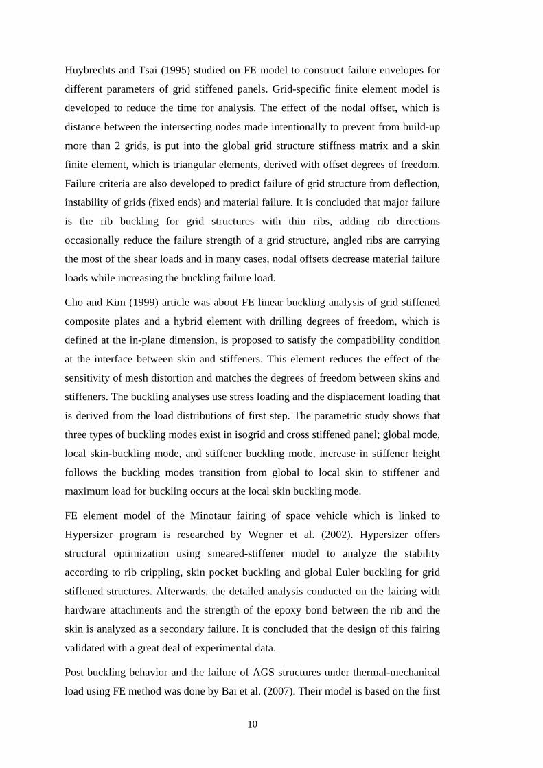
Huybrechts and Tsai (1995) studied on FE model to construct failure envelopes for
different parameters of grid stiffened panels. Grid-specific finite element model is
developed to reduce the time for analysis. The effect of the nodal offset, which is
distance between the intersecting nodes made intentionally to prevent from build-up
more than 2 grids, is put into the global grid structure stiffness matrix and a skin
finite element, which is triangular elements, derived with offset degrees of freedom.
Failure criteria are also developed to predict failure of grid structure from deflection,
instability of grids (fixed ends) and material failure. It is concluded that major failure
is the rib buckling for grid structures with thin ribs, adding rib directions
occasionally reduce the failure strength of a grid structure, angled ribs are carrying
the most of the shear loads and in many cases, nodal offsets decrease material failure
loads while increasing the buckling failure load.
Cho and Kim (1999) article was about FE linear buckling analysis of grid stiffened
composite plates and a hybrid element with drilling degrees of freedom, which is
defined at the in-plane dimension, is proposed to satisfy the compatibility condition
at the interface between skin and stiffeners. This element reduces the effect of the
sensitivity of mesh distortion and matches the degrees of freedom between skins and
stiffeners. The buckling analyses use stress loading and the displacement loading that
is derived from the load distributions of first step. The parametric study shows that
three types of buckling modes exist in isogrid and cross stiffened panel; global mode,
local skin-buckling mode, and stiffener buckling mode, increase in stiffener height
follows the buckling modes transition from global to local skin to stiffener and
maximum load for buckling occurs at the local skin buckling mode.
FE element model of the Minotaur fairing of space vehicle which is linked to
Hypersizer program is researched by Wegner et al. (2002). Hypersizer offers
structural optimization using smeared-stiffener model to analyze the stability
according to rib crippling, skin pocket buckling and global Euler buckling for grid
stiffened structures. Afterwards, the detailed analysis conducted on the fairing with
hardware attachments and the strength of the epoxy bond between the rib and the
skin is analyzed as a secondary failure. It is concluded that the design of this fairing
validated with a great deal of experimental data.
Post buckling behavior and the failure of AGS structures under thermal-mechanical
load using FE method was done by Bai et al. (2007). Their model is based on the first
10
order shear theory under the assumption of Von Karman non-linear deformation.
Progressive failure, buckling, large deformation and local failure modes in AGS
structure is taken into account for their study. It is concluded that stiffness
degradation caused by progressive failure of the stiffeners.
Meink (n.d) studied on a comparison of composite grid and composite sandwich
shroud using FE modeling. He used IDEAS to run global buckling and deflection
solution. FE model used in this study can only use smeared stiffener laminate for
material failure and global buckling properties.
Chen and Tsai (1996) study was about FEM technique that can be adapted to the
integrated equivalent stiffness model using Mindlin’s theory. Exact FEM modeling,
that uses the equivalent stiffness model, can obtain a refined stress analysis with high
precision. SDRC I-DEAS code is used to check stresses and local buckling from
FEM analysis.
Buckling of isogrid plates using FE modeling was also investigated by Lavin and
Miravete (2010). FE models are developed using COMSOL Multiphysics to predict
buckling modes.
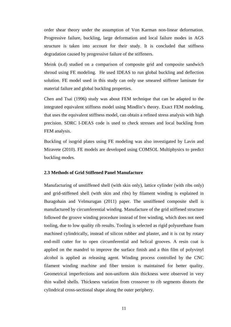
2.3 Methods of Grid Stiffened Panel Manufacture
Manufacturing of unstiffened shell (with skin only), lattice cylinder (with ribs only)
and grid-stiffened shell (with skin and ribs) by filament winding is explained in
Buragohain and Velmurugan (2011) paper. The unstiffened composite shell is
manufactured by circumferential winding. Manufacture of the grid stiffened structure
followed the groove winding procedure instead of free winding, which does not need
tooling, due to low quality rib results. Tooling is selected as rigid polyurethane foam
machined cylindrically, instead of silicon rubber and plaster, and it is cut by rotary
end-mill cutter for to open circumferential and helical grooves. A resin coat is
applied on the mandrel to improve the surface finish and a thin film of polyvinyl
alcohol is applied as releasing agent. Winding process controlled by the CNC
filament winding machine and fiber tension is maintained for better quality.
Geometrical imperfections and non-uniform skin thickness were observed in very
thin walled shells. Thickness variation from crossover to rib segments distorts the
cylindrical cross-sectional shape along the outer periphery.
11
Huybrechts et al. (n.d.) listed the proven manufacturing methods, which show the
actual grid stricture behavior, from the vast number of literature;
• Wet winding (the Brute Force Approach),
• Wet winding around pins by Russian researchers,
• Wet winding in hard tooling with E-Beam cure by Boeing,
• Nodal spreading by Stanford University,
• Winding into solid rubber tooling by Philips Lab,
• The hybrid tooling method by Air Force Research Laboratory (AFRL),
• Fiber placement with hybrid tooling by AFRL & Boeing,
• Fiber placement with expansion inserts by Alliant Tech Systems,
• The located expansion tooling method by AFRL & Boeing,
• The SnapSnat method by Composite Optics,
• The RIG method by Stanford University.
It is also stated a couple of automated methods to manufacture AGS structures.
Philips laboratory used solid cured silicon rubber sheets wrapped around metallic
mandrels for cylindrical sections. Rib intersections have the build-up problem that
also affects the continuity of the fiber. High coefficient of thermal expansion (CTE)
of silicon rubber provides expansion at curing temperature of the ribs to prevent the
fiber sparse areas especially near the nodes. Rib quality near these regions is
significantly low without consolidation of the ribs provided by the lateral expansion
by silicon rubber. The drawbacks of expansion block method are the lack of control
over the compaction caused by silicon rubber, warping of tooling due to high CTE,
high thermal/mechanical stresses in the finished part and difficulty in producing
more complex shapes to have proper groove alignment.
Hybrid tooling method tries solving these problems, which is explained in previous
paragraph, with addition of expansion tooling inserts in a thermally stable base tool.
This method provides precise control of lateral rib compaction and it can be applied
to complex shapes without the problems of groove alignment or helix angle of rib.
This study also captures manufacture of payload shroud using hybrid tooling method
with 5-Axis filament winding machine. Three parts are used to build this method are
stainless steel base mandrel, base tooling material and silicon rubber expansion
inserts (Huybrechts and Meink, n.d.).
12
Huybrechts et al. (2002) mentioned about the problem of almost all manufacturing
methods of AGS structures that is nodal build-up. This build-up nodal points cause
loss of strength, stiffness and modeling accuracy. Two stable tooling concepts are
explained:
• Hybrid tooling has base tool and silicon rubber expansion tool. The base tool
is cut to make grooves for rib directions and an expansion block, which is
silicon rubber, is put into these grooves to provide consolidation for the
woven fibers at the high temperature curing phase.
• Expansion block tooling has advantage to apply for different rib geometries.
It has a base tool, which is stiff and stable, and expansion blocks with high
coefficient of thermal expansion (CTE). Lateral compaction for the ribs is
provided by expansion blocks.
Kim (2000) studied on fabrication of thin composite isogrid stiffened panel. Nodal
offset is used for to reduce build-up effect on the manufacturing and the empty space
due to nodal offset is filled with the resin. The advantage of filling with resin is
stronger skin to rib bonding and possible mounting points such as hinges and
electronic equipment.
In fabrication, metal isogrid tool used to cast silicon rubber mold and steel base plate
is covered with borders to constrain the rubber from expanding at high temperatures.
All the fibers laid into grooves between silicon rubber and steel caul plate used at the
top of the skin to obtain good compaction.
Dutta (1998) summarized manufacturing methods of composite grids. The major
considerations about manufacturing of composite grid structures; all ribs has to be
unidirectional, rib cross-section must be well defined and nodes must have
continuous fibers.
Composite grids are initially manufactured based on traditional slotted joint
manufacturing system at Stanford University. The composite grids, which will be
slotted afterwards, are manufactured using pultruded thin unidirectional sections. The
disadvantages of this process include, cost of machining slots, difficulty on
assemblage of ribs having multiple slotted ribs, loss of stiffness and strength due to
machined slots and imperfect fit at slotted joints, and limited grid configuration as
square or rectangular. The upper limit of the fiber volume fraction in the ribs is
13
controlled by the node sections, generally 60 percent and 30 percent at the ribs.
Application of node offset method can increase the fiber fraction in the ribs. The
fiber fraction can be increased further by designing nodes wider and it will reduce
the thickness of interlacing layers.
Direct crossover interlaced joints method use the wet winding process and at the
node section fibers are continuous and crossing over each other. Fibers at the joints
were consolidated periodically by hand to maximize compaction and fiber volume.
The silicon rubber mold provided good compaction and consolidation during curing
of the product.
Stanford Pin Enhanced Geometry (PEG) Process is a modified process of direct
crossover interlaced joints, which has resin pool, fiber warping, and wrinkle problem.
In this method central pin node without any lead angle and a pattern with 1.3 degree
lead angle to smoothen the rib-node transition are used. Alternating placement and
laminated lay-up pattern are used but this does not provide reduction on the node
thickness to rib thickness and the single pin in the middle disturbs the fibers and
causes dry zones. A follow-up modification of four pin instead of one pin used to
have better specimen. In later attempts, fibers are forced to conform properly during
cure cycle but resin pool, fiber undulations, wrinkles remained and resin poor regions
in the nodes appeared.
Stanford Tooling-Reinforced Interlaced Grid (TRIG) Process is a process developed
for the flat orthogrid. This method changes conventional concept of tooling by using
it as integral part of the finished structure. Similar mold blocks, which are used for
PEG method, are also used for TRIG. Tooling blocks are placed on the wooden base
plate with guiding lines and vacuum bag film for easy separation. Tooling blocks are
filament-wound composite tube segments with outer cross sectional geometry
becoming the grid channel geometry. Nails are positioned at the ends of each channel
to provide fiber tension and continuity. Wetted fibers are wound into channels
between tooling blocks and then waited until resin is cured. The disadvantage of
TRIG involves direct crossover in the nodes, the open inspection of molded grids is
not possible, and the integrated tooling increases weight.
A demonstration of current technology revealed that composite grids generally suffer
from manufacturing problems of low density interlacing, no fiber tension, and
excessively thick nodes with direct roving crossovers (Dutta, 1998).
14
2.4 Optimization of Grid Stiffened Panels
Optimization of grid stiffened panels is mandatory to find the best configuration
inside the design space. Design space includes all kind of failure types and
dimensioning, thus expectation is to search a point which is converging at the
optimum. Thus optimization models are designed and run with intrinsic algorithms
as it is referenced in this section.
Chen and Tsai (1996) is studied on the optimization of the composite grid structures.
Their design space include grids with or without skins, orthotropic grids that consist
0, 90, and ±𝜃° directional ribs, rectangular ribs with equal height, symmetric skin
laminate lay-up. Loading conditions are hygrothermal and multiple mechanical. The
failure modes are material failure and the local buckling of skins and ribs. Direct
search method, which is a solution method for the problems that does not require any
information about the gradient of the objective function, is selected.
Optimization of the curvilinear (alignment) stiffeners on different loading conditions
is studied by Mulani et al. (2011). Gradient based and/or global optimizations are
developed to minimize the mass, and constrains are buckling, Von Misses stress, and
crippling or local failure of the stiffener. Design variables are orientation, the shape
of the stiffeners, the spacing between the stiffeners, stiffeners thickness and height,
and thickness of the plate. An optimization framework is created using MD-
PATRAN (Geometry Modeling), MD-NASTRAN (FEM Analysis), VisualDOC
(External Optimizer) and MATLAB (Central Processor) to optimize the stiffened
panels using grid-stiffening concept and the curvilinear stiffeners.
Wodesenbet (2003) used equivalent stiffness of the shell/stiffener to optimize the
grid stiffened composite panels. Parametric study is performed on the different
design variables, which are shell thickness, shell winding angle, longitudinal
modulus and stiffeners orientation angle and their effect on buckling load is
presented. Increase in skin thickness results in higher buckling resistance of stiffened
structure. The effect of stiffener orientation angle and longitudinal modulus increase
also results in higher buckling resistance of the stiffened cylinder structure.
Akl et al. (2008) studied on optimization of iso-grid stiffened plate for the static and
dynamic characteristic of these plates/stiffeners assemblies. Static part of
optimization tries to maximize critical buckling load of the iso-grid plate, while
15
dynamic part of optimization tries to maximize multiple natural frequencies of the
stiffened plate. A FE model is developed for Mindlin plates with arbitrary stiffeners
and this model is used as a basis for optimization of critical buckling load and natural
frequencies of stiffened plate. The plate is modeled using an 8-node isoparametric
element, which is formulated using the first-order shear deformation theory and the
stiffeners are modeled using a 3-node element based on the Timoshenko beam
theory. Using this approach, stiffeners located arbitrary along a plate structure can be
easily modeled without the need to change the ground mesh of the plate model. The
analysis to maximize the first six critical buckling loads resulted in optimum stiffener
inclination angle of 35°.
Phillips and Gürdal (1990) research was about optimum design of the geodesic
panels (diagonal and cross) and the longitudinally stiffened panels to achieve
minimum weight. The design variables are skin thickness (quasi–isotropic laminate),
stiffener height, and stiffener thickness and increasing number of stiffened cells used
for panel configuration. Uniaxial compression, pure shear and combined
compression-shear loads are applied. PANSYS is used to seek minimum-weight
wing rib designs subject to constraints on both buckling resistance and material
strength. It is concluded that under compression loading diagonal and cross
geodesically stiffened panels are lighter than the longitudinally stiffened panel and
minimum mass achieved at higher number of stiffened cells, under shear loading it
gives almost similar results and cross stiffened panel appears to be most feasible
design and under compression-shear loading.
16
3. THEORETICAL MODEL AND FUNDAMENTAL EQUATIONS
Theoretical model is derived from the classical laminate theory in this chapter. Intersecting nodes material properties and failure strength is defined in detail. Extensional, coupling, and bending stiffness matrices for composite parts are calculated. Additionally, failure mechanisms, i.e. stiffener crippling, Euler buckling, is studied for to implement the analytical equations into optimization cycle.
3.1 Classical Laminate Theory
A lamina is a thin layer of a composite structure and a laminate is formed by stacking
a number of laminae. Mechanical analysis of a lamina follows the way of
computation for to reach properties of the laminate. A lamina is not an isotropic
homogenous material. The lamina consists of two parts; first is isotropic
homogenous fibers and second is an isotropic homogeneous matrix. The different
stiffness properties of points in the lamina originate from its location, which is in the
fiber, the matrix, or the fiber-matrix interface. The difficulty of mechanical modeling
of the lamina leads to macro-mechanical analysis based on average properties and
consideration of homogeneous laminate. However, mechanical behavior of the
lamina is still different than homogeneous isotropic material (Kaw, 2006).
The unidirectional fiber-reinforced composite is treated as a two-phase material, with
the axis of the reinforcing fibers aligned parallel and packed randomly in the plane
transverse to the fiber axis. The governing constitutive equation of this composite is
the generalized Hooke's law. The material coefficients of this equation are expressed
as functions of the material and geometric parameters of the constituent materials.
The laminated composite is assembled by bonding together unidirectional layers of
identical mechanical properties, with adjacent layers orthogonal to each other (cross-
ply) or oriented symmetrically with respect to an arbitrary reference axis (angle-ply).
The governing constitutive equation is the relation between the in-plane stress and
moment and the in-plane strain and curvature. The material coefficients of this
17
equation are expressed as functions of the properties of the unidirectional composite
and lamination parameters (Tsai, n.d.).
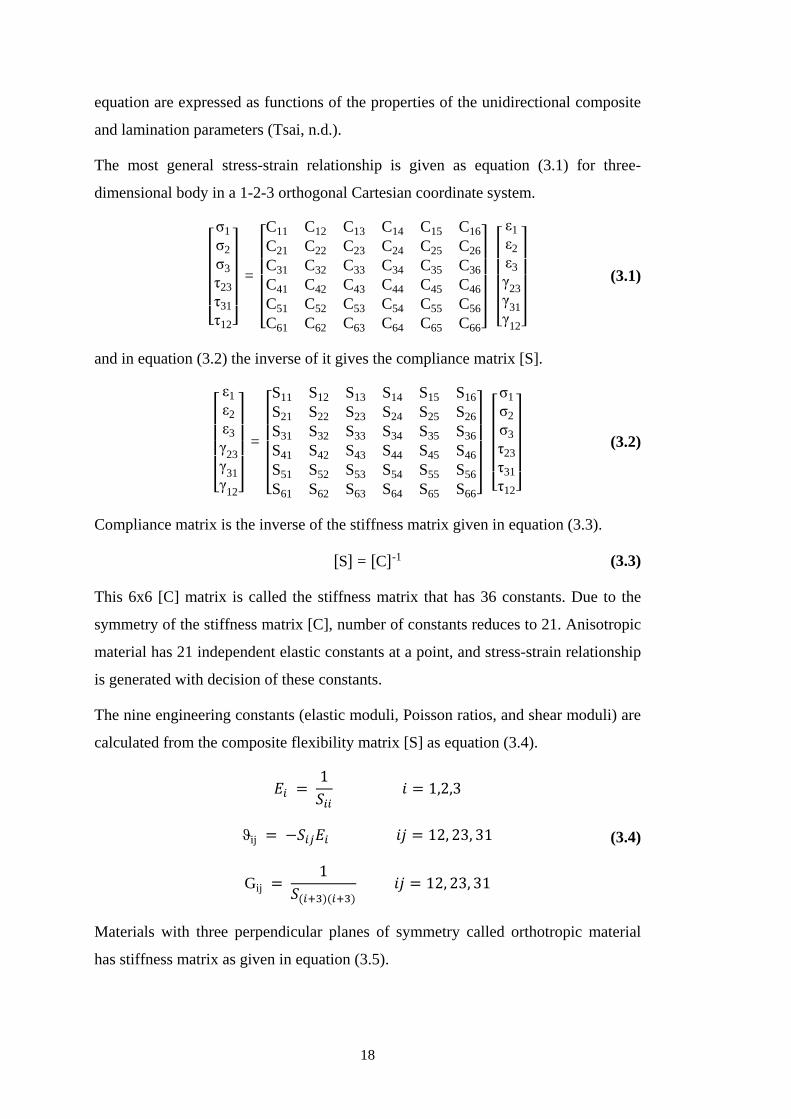
The most general stress-strain relationship is given as equation (3.1) for three-
dimensional body in a 1-2-3 orthogonal Cartesian coordinate system.
and in equation (3.2) the inverse of it gives the compliance matrix [S].
Compliance matrix is the inverse of the stiffness matrix given in equation (3.3).
This 6x6 [C] matrix is called the stiffness matrix that has 36 constants. Due to the
symmetry of the stiffness matrix [C], number of constants reduces to 21. Anisotropic
material has 21 independent elastic constants at a point, and stress-strain relationship
is generated with decision of these constants.
The nine engineering constants (elastic moduli, Poisson ratios, and shear moduli) are
calculated from the composite flexibility matrix [S] as equation (3.4).
Materials with three perpendicular planes of symmetry called orthotropic material
has stiffness matrix as given in equation (3.5).
⎣⎢⎢⎢⎢⎡σ1σ2σ3τ23τ31τ12⎦⎥⎥⎥⎥⎤
=
⎣⎢⎢⎢⎢⎡C11 C12 C13 C14 C15 C16C21 C22 C23 C24 C25 C26C31 C32 C33 C34 C35 C36C41 C42 C43 C44 C45 C46C51 C52 C53 C54 C55 C56C61 C62 C63 C64 C65 C66⎦
⎥⎥⎥⎥⎤
⎣⎢⎢⎢⎢⎡
ε1ε2ε3γ23γ31γ12⎦⎥⎥⎥⎥⎤
(3.1)
⎣⎢⎢⎢⎢⎡
ε1ε2ε3γ23γ31γ12⎦⎥⎥⎥⎥⎤
=
⎣⎢⎢⎢⎢⎡S11 S12 S13 S14 S15 S16S21 S22 S23 S24 S25 S26S31 S32 S33 S34 S35 S36S41 S42 S43 S44 S45 S46S51 S52 S53 S54 S55 S56S61 S62 S63 S64 S65 S66⎦
⎥⎥⎥⎥⎤
⎣⎢⎢⎢⎢⎡σ1σ2σ3τ23τ31τ12⎦⎥⎥⎥⎥⎤
(3.2)
[S] = [C]-1 (3.3)
𝐸𝑖 = 1𝑆𝑖𝑖
𝑖 = 1,2,3
ϑij = −𝑆𝑖𝑗𝐸𝑖 𝑖𝑗 = 12, 23, 31
Gij = 1
𝑆(𝑖+3)(𝑖+3) 𝑖𝑗 = 12, 23, 31
(3.4)
18
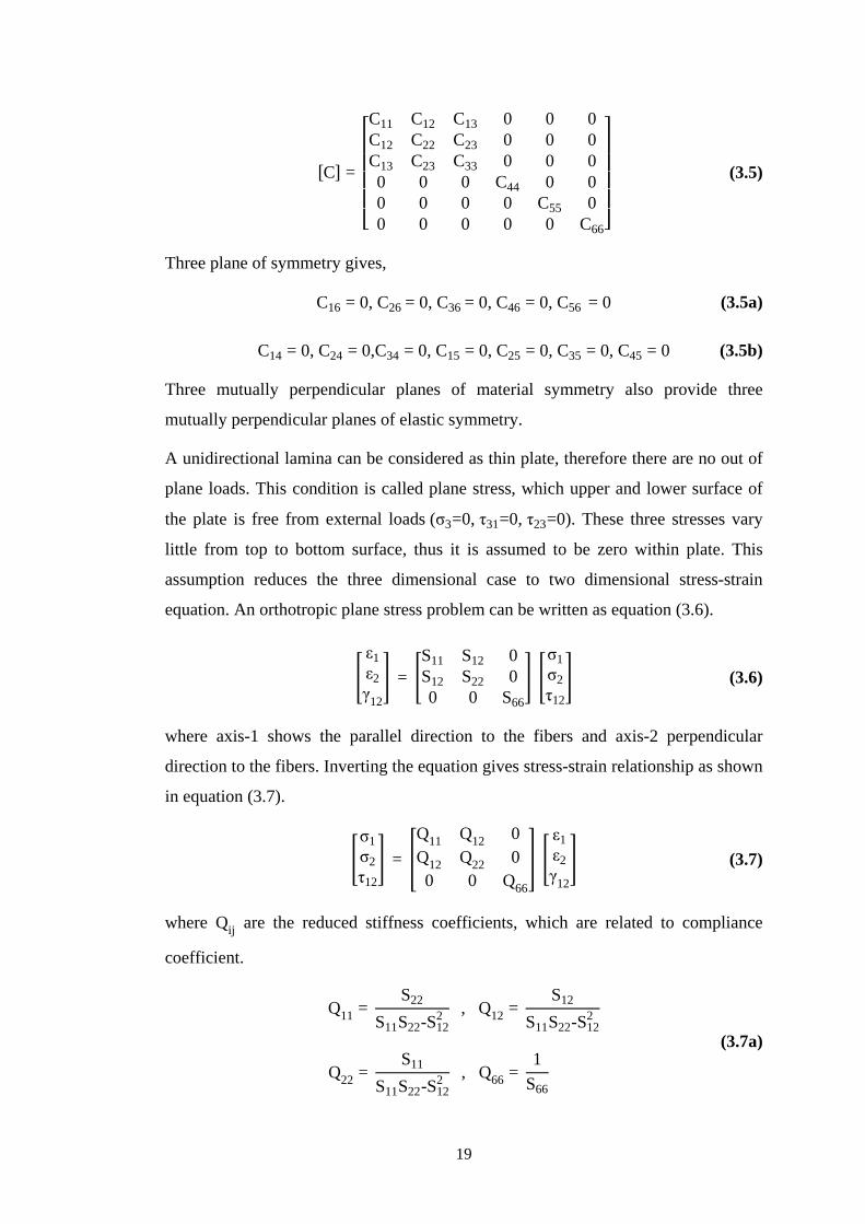
Three plane of symmetry gives,
Three mutually perpendicular planes of material symmetry also provide three
mutually perpendicular planes of elastic symmetry.
A unidirectional lamina can be considered as thin plate, therefore there are no out of
plane loads. This condition is called plane stress, which upper and lower surface of
the plate is free from external loads (σ3=0, τ31=0, τ23=0). These three stresses vary
little from top to bottom surface, thus it is assumed to be zero within plate. This
assumption reduces the three dimensional case to two dimensional stress-strain
equation. An orthotropic plane stress problem can be written as equation (3.6).
where axis-1 shows the parallel direction to the fibers and axis-2 perpendicular
direction to the fibers. Inverting the equation gives stress-strain relationship as shown
in equation (3.7).
where Qij are the reduced stiffness coefficients, which are related to compliance
coefficient.
[C] =
⎣⎢⎢⎢⎢⎡C11 C12 C13 0 0 0C12 C22 C23 0 0 0C13 C23 C33 0 0 00 0 0 C44 0 00 0 0 0 C55 00 0 0 0 0 C66⎦
⎥⎥⎥⎥⎤
(3.5)
C16 = 0, C26 = 0, C36 = 0, C46 = 0, C56 = 0 (3.5a)
C14 = 0, C24 = 0,C34 = 0, C15 = 0, C25 = 0, C35 = 0, C45 = 0 (3.5b)
�ε1ε2γ12
� = �S11 S12 0S12 S22 00 0 S66
� �σ1σ2τ12
� (3.6)
�σ1σ2τ12
� = �Q11 Q12 0Q12 Q22 00 0 Q66
� �ε1ε2γ12
� (3.7)
Q11 = S22
S11S22-S122 , Q12 =
S12
S11S22-S122
Q22 = S11
S11S22-S122 , Q66 =
1S66
(3.7a)
19
The above equations give the properties for unidirectional fibers but most of the time
some laminae are placed at an angle for to provide higher stiffness and strength
properties in the transverse direction. Angle lamina can be defined in its own local
coordinate system or material coordinate system (1-2 coordinate system), and then
the properties can be translated into global coordinate system (x-y coordinate
system). The angle between two coordinate systems is denoted by an angle θ.
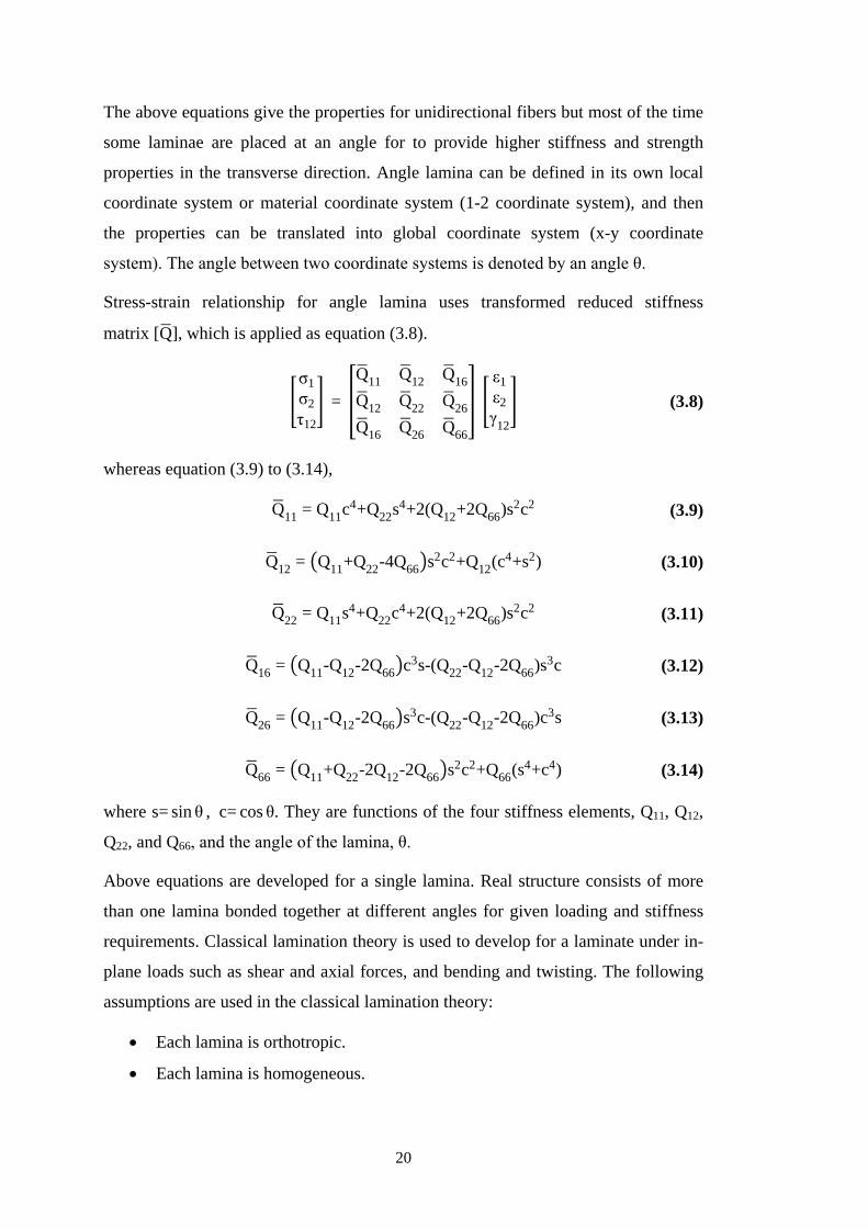
Stress-strain relationship for angle lamina uses transformed reduced stiffness
matrix [Q�], which is applied as equation (3.8).
whereas equation (3.9) to (3.14),
where s= sin θ , c= cos θ. They are functions of the four stiffness elements, Q11, Q12,
Q22, and Q66, and the angle of the lamina, θ.
Above equations are developed for a single lamina. Real structure consists of more
than one lamina bonded together at different angles for given loading and stiffness
requirements. Classical lamination theory is used to develop for a laminate under in-
plane loads such as shear and axial forces, and bending and twisting. The following
assumptions are used in the classical lamination theory:
• Each lamina is orthotropic.
• Each lamina is homogeneous.
�σ1σ2τ12
� = �Q�11 Q�12 Q�16
Q�12 Q�22 Q�26Q�16 Q�26 Q�66
� �ε1ε2γ12
� (3.8)
Q�11 = Q11c4+Q22s4+2(Q12+2Q66)s2c2 (3.9)
Q�12 = �Q11+Q22-4Q66�s2c2+Q12(c4+s2) (3.10)
Q�22 = Q11s4+Q22c4+2(Q12+2Q66)s2c2 (3.11)
Q�16 = �Q11-Q12-2Q66�c3s-(Q22-Q12-2Q66)s3c (3.12)
Q�26 = �Q11-Q12-2Q66�s3c-(Q22-Q12-2Q66)c3s (3.13)
Q�66 = �Q11+Q22-2Q12-2Q66�s2c2+Q66(s4+c4) (3.14)
20
• A line straight and perpendicular to the middle surface remains straight and
perpendicular to the middle surface during deformation (γxz=γyz=0).
• The laminate is thin and is loaded only in its plane (plane
stress) (σz=τxz=τyz=0).
• Displacements are continuous and small throughout the
laminate (|u|, |v|, |w|≪|h|), where h is the laminate thickness.
• Each lamina is elastic.
• No slip occurs between the lamina interfaces.
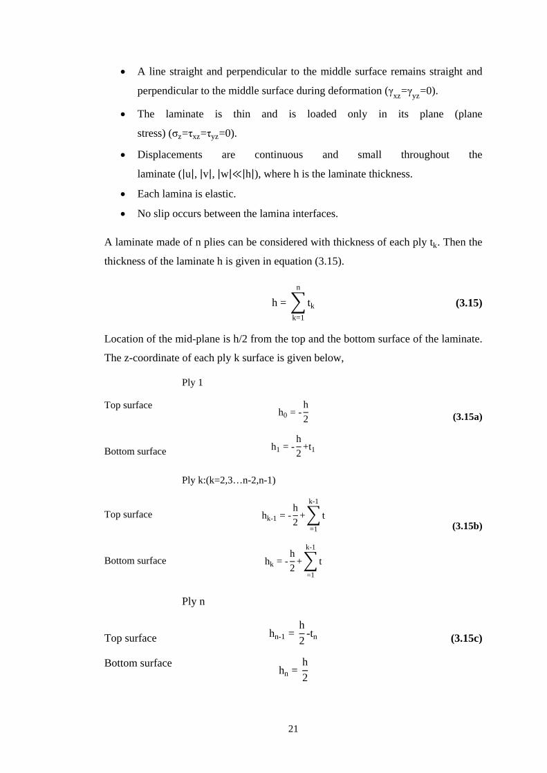
A laminate made of n plies can be considered with thickness of each ply tk. Then the
thickness of the laminate h is given in equation (3.15).
Location of the mid-plane is h/2 from the top and the bottom surface of the laminate.
The z-coordinate of each ply k surface is given below,
h = � tk
n
k=1
(3.15)
Top surface
Bottom surface
Ply 1
h0 = -h2
h1 = -h2
+t1
(3.15a)
Top surface
Bottom surface
Ply k:(k=2,3…n-2,n-1)
hk-1 = -h2
+� tk-1
=1
hk = -h2
+� tk-1
=1
(3.15b)
Top surface
Bottom surface
Ply n
hn-1 = h2
-tn
hn = h2
(3.15c)
21
Then, global stresses in each lamina can be integrated, and the resultant forces and
the resultant moments per unit length in the x-y plane through the laminate thickness
can be found. The resultant force and moments can be written in terms of mid-plane
strains and curvatures and also the transformed reduced stiffness matrix, [Q�], can be
combined into equation. Then, the [A], [B], [D] matrices, which are called the
extensional, coupling, and bending stiffness matrices respectively, can be written as
equation (3.16) to (3.18).
The forces applied to a small part of the laminate, can be described by 6 components
in classical shell theory, 3 in-plane forces and 3 moments. Generalized constitutive
equation (3.19) far any laminate have form.
where,
Aij = ���Q� ij��k(hk-hk-1)
n
k=1
, i = 1,2,6; j = 1,2,6 (3.16)
Bij = 12���Q� ij��k
(hk2-hk-1
2)n
k=1
, i = 1,2,6; j = 1,2,6 (3.17)
Dij = 13���Q� ij��k
(hk3-hk-1
3), i = 1,2,6; j = 1,2,6n
k=1
(3.18)
⎣⎢⎢⎢⎢⎢⎡
NxNyNxyMxMyMxy⎦
⎥⎥⎥⎥⎥⎤
=
⎣⎢⎢⎢⎢⎡A11 A12 A16 B11 B12 B16A12 A22 A26 B12 B22 B26A16 A26 A66 B16 B26 B66B11 B12 B16 D11 D12 D16B12 B22 B26 D12 D22 D26B16 B26 B66 D16 D26 D66⎦
⎥⎥⎥⎥⎤
⎣⎢⎢⎢⎢⎢⎡ εx
0
εy0
γxy0
κxκyκxy⎦
⎥⎥⎥⎥⎥⎤
(3.19)
Nx, Ny = normal force per unit length
Nxy = shear force per unit length
Mx, My = bending moments per unit length
Mxy = twisting moment per unit length
(3.19a)
22
Symmetric laminates have no membrane-stretching coupling behavior that makes [B]
coupling matrix zero. Denoting the inverse of the [A] matrix by [a] and the inverse of
the [D] matrix by equation (3.20) become for symmetric laminate.
3.1.1 Material property of intersecting nodes
Stiffener properties of the AGS structure are not constant along its length due to
nodal build-ups. Total number of fibers increases two or more than two times at node
points based on nodal offset decision of the design, thus fiber volume fraction
increases up to 80 percent. Moreover, fibers that are crossing over each other at
nodes have different material axis direction depending on the pattern of the AGS
application. These nodal section characteristics of the AGS panel need to be defined
in one ply, which has to provide continuity along all the stiffeners (Kassapoglou,
2013).
According to the angles of intersecting grids, equivalent symmetric lay-ups are used
to include the different material axes into one by using in-plane properties taken from
Equation. Equations are used to develop effective in-plane properties as equations
(3.21) to (3.25).
⎣⎢⎢⎢⎢⎢⎡ εx
0
εy0
γxy0
κxκyκxy⎦
⎥⎥⎥⎥⎥⎤
=
⎣⎢⎢⎢⎢⎡a11 a12 a16 0 0 0a12 a22 a26 0 0 0a16 a26 a66 0 0 00 0 0 d11 d12 d160 0 0 d12 d22 d260 0 0 d16 d26 d66⎦
⎥⎥⎥⎥⎤
⎣⎢⎢⎢⎢⎢⎡
NxNyNxyMxMyMxy⎦
⎥⎥⎥⎥⎥⎤
(3.20)
Ex = 1
ha11 (3.21)
Ey = 1
ha22 (3.22)
Gxy = 1
ha66 (3.23)
ϑxy = -a12
a11 (3.24)
23
and orthotropic 3D symmetry relations comply with equations (3.26) and (3.27).
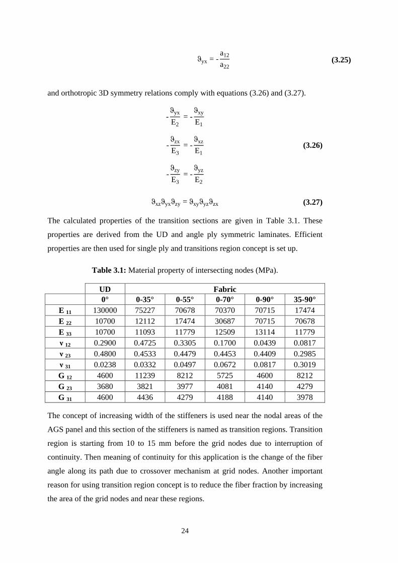
The calculated properties of the transition sections are given in Table 3.1. These
properties are derived from the UD and angle ply symmetric laminates. Efficient
properties are then used for single ply and transitions region concept is set up.
Table 3.1: Material property of intersecting nodes (MPa).
The concept of increasing width of the stiffeners is used near the nodal areas of the
AGS panel and this section of the stiffeners is named as transition regions. Transition
region is starting from 10 to 15 mm before the grid nodes due to interruption of
continuity. Then meaning of continuity for this application is the change of the fiber
angle along its path due to crossover mechanism at grid nodes. Another important
reason for using transition region concept is to reduce the fiber fraction by increasing
the area of the grid nodes and near these regions.
ϑyx = -a12
a22 (3.25)
-ϑyx
E2 = -
ϑxy
E1
-ϑzx
E3 = -
ϑxz
E1
-ϑzy
E3 = -
ϑyz
E2
(3.26)
ϑxzϑyxϑzy = ϑxyϑyzϑzx (3.27)
UD Fabric
0° 0-35° 0-55° 0-70° 0-90° 35-90° E 11 130000 75227 70678 70370 70715 17474 E 22 10700 12112 17474 30687 70715 70678 E 33 10700 11093 11779 12509 13114 11779 ν 12 0.2900 0.4725 0.3305 0.1700 0.0439 0.0817 ν 23 0.4800 0.4533 0.4479 0.4453 0.4409 0.2985 ν 31 0.0238 0.0332 0.0497 0.0672 0.0817 0.3019 G 12 4600 11239 8212 5725 4600 8212 G 23 3680 3821 3977 4081 4140 4279 G 31 4600 4436 4279 4188 4140 3978
24
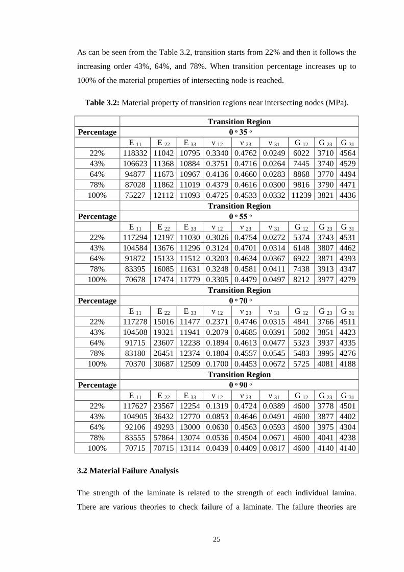
As can be seen from the Table 3.2, transition starts from 22% and then it follows the
increasing order 43%, 64%, and 78%. When transition percentage increases up to
100% of the material properties of intersecting node is reached.
Table 3.2: Material property of transition regions near intersecting nodes (MPa).
3.2 Material Failure Analysis
The strength of the laminate is related to the strength of each individual lamina.
There are various theories to check failure of a laminate. The failure theories are
Transition Region Percentage 0 ͦ 35 ͦ
E 11 E 22 E 33 ν 12 ν 23 ν 31 G 12 G 23 G 31 22% 118332 11042 10795 0.3340 0.4762 0.0249 6022 3710 4564 43% 106623 11368 10884 0.3751 0.4716 0.0264 7445 3740 4529 64% 94877 11673 10967 0.4136 0.4660 0.0283 8868 3770 4494 78% 87028 11862 11019 0.4379 0.4616 0.0300 9816 3790 4471 100% 75227 12112 11093 0.4725 0.4533 0.0332 11239 3821 4436
Transition Region Percentage 0 ͦ 55 ͦ
E 11 E 22 E 33 ν 12 ν 23 ν 31 G 12 G 23 G 31 22% 117294 12197 11030 0.3026 0.4754 0.0272 5374 3743 4531 43% 104584 13676 11296 0.3124 0.4701 0.0314 6148 3807 4462 64% 91872 15133 11512 0.3203 0.4634 0.0367 6922 3871 4393 78% 83395 16085 11631 0.3248 0.4581 0.0411 7438 3913 4347 100% 70678 17474 11779 0.3305 0.4479 0.0497 8212 3977 4279
Transition Region Percentage 0 ͦ 70 ͦ
E 11 E 22 E 33 ν 12 ν 23 ν 31 G 12 G 23 G 31 22% 117278 15016 11477 0.2371 0.4746 0.0315 4841 3766 4511 43% 104508 19321 11941 0.2079 0.4685 0.0391 5082 3851 4423 64% 91715 23607 12238 0.1894 0.4613 0.0477 5323 3937 4335 78% 83180 26451 12374 0.1804 0.4557 0.0545 5483 3995 4276 100% 70370 30687 12509 0.1700 0.4453 0.0672 5725 4081 4188
Transition Region Percentage 0 ͦ 90 ͦ
E 11 E 22 E 33 ν 12 ν 23 ν 31 G 12 G 23 G 31 22% 117627 23567 12254 0.1319 0.4724 0.0389 4600 3778 4501 43% 104905 36432 12770 0.0853 0.4646 0.0491 4600 3877 4402 64% 92106 49293 13000 0.0630 0.4563 0.0593 4600 3975 4304 78% 83555 57864 13074 0.0536 0.4504 0.0671 4600 4041 4238 100% 70715 70715 13114 0.0439 0.4409 0.0817 4600 4140 4140
25
based on stresses in the material or local axes due to orthotropic characteristic of the
composite structures. A unidirectional (UD) lamina has two directions for its own
material axes, thus there are four normal strength parameters existing for tension case
and compression case. The fifth strength parameter, which can be positive or
negative, is the shear strength of UD lamina. The sign of the shear stress has no
effect on the strength of the UD lamina but for angle lamina sign of shear stress
affect the strength properties. The five strength parameters are given for UD lamina
as follow.
For an angle lamina, first stresses in the local axes are found and then these
parameters are compared to local stresses to find whether lamina has failed (Kaw,
2006).
Maximum Stress Failure Theory is used in FE optimization for material failure.
Failure is predicted in a lamina by comparing the normal and the shear stresses in the
local axes, and corresponding ultimate strengths of the unidirectional lamina. Lamina
is considered to be failed if,
is violated. Here is negative sign is added to indicate compressive stresses. All the
components are compared with corresponding strengths, thus there is no interaction
with others.
Failure strength of CFRP is calculated using maximum stress failure theory for UD
and intersecting nodes given in Table 3.3.
�σ1T�
ult = Ultimate longitudinal tensile strength (direction 1)
�σ1C�
ult = Ultimate longitudinal compressive strength (direction 1)
�σ2T�
ult = Ultimate transverse tensile strength (direction 2)
�σ2C�
ult = Ultimate transverse compressive strength (direction 2)
(τ12)ult = Ultimate in-plane shear strength (plane 12)
(3.28a)
-�σ1C�
ult< σ1 < �σ1
T�ult
, or
-�σ2C�
ult< σ2 < �σ2
T�ult
, or
-(τ12)ult< τ12 < (τ12)ult
(3.28b)
26
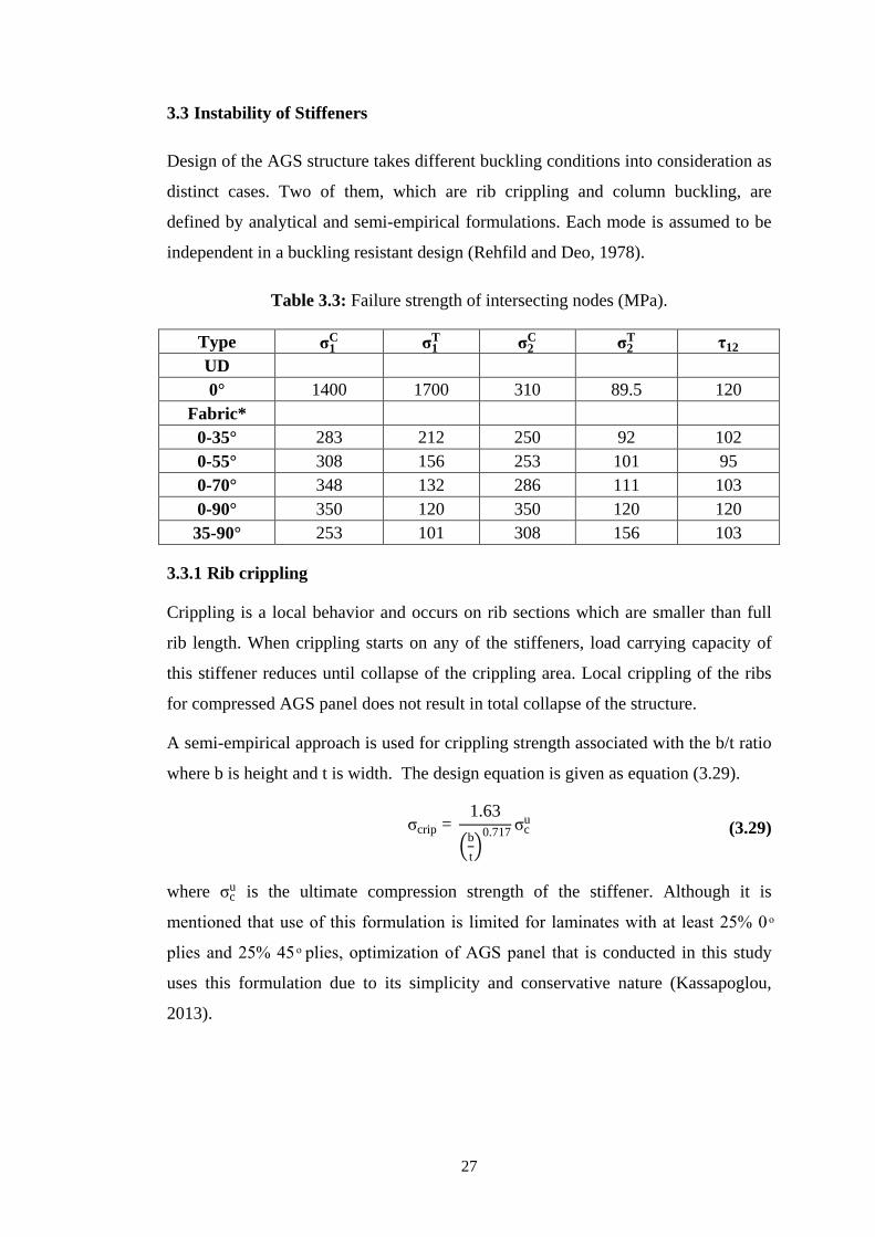
3.3 Instability of Stiffeners
Design of the AGS structure takes different buckling conditions into consideration as
distinct cases. Two of them, which are rib crippling and column buckling, are
defined by analytical and semi-empirical formulations. Each mode is assumed to be
independent in a buckling resistant design (Rehfild and Deo, 1978).
Table 3.3: Failure strength of intersecting nodes (MPa).
3.3.1 Rib crippling
Crippling is a local behavior and occurs on rib sections which are smaller than full
rib length. When crippling starts on any of the stiffeners, load carrying capacity of
this stiffener reduces until collapse of the crippling area. Local crippling of the ribs
for compressed AGS panel does not result in total collapse of the structure.
A semi-empirical approach is used for crippling strength associated with the b/t ratio
where b is height and t is width. The design equation is given as equation (3.29).
where σcu is the ultimate compression strength of the stiffener. Although it is
mentioned that use of this formulation is limited for laminates with at least 25% 0 ͦ
plies and 25% 45 ͦ plies, optimization of AGS panel that is conducted in this study
uses this formulation due to its simplicity and conservative nature (Kassapoglou,
2013).
Type σ1C σ1
T σ2C σ2
T τ12 UD 0° 1400 1700 310 89.5 120
Fabric* 0-35° 283 212 250 92 102 0-55° 308 156 253 101 95 0-70° 348 132 286 111 103 0-90° 350 120 350 120 120 35-90° 253 101 308 156 103
σcrip = 1.63
�bt�
0.717 σcu (3.29)
27
3.3.2 Column buckling
Column buckling load of stiffeners can be computed from the Euler buckling
analysis of beams. The difference of column buckling from crippling is that stiffener
buckles at full length and it results in total collapse of stiffener between two nodes.
Although substantial build-up of material at the nodes and effective increase in rib
with near nodes makes boundary conditions equivalent to full clamping, the pinned
end boundary is taken as the buckling case to keep conservative result. The famous
equation of column buckling of pinned end beam is given as equation (3.30).
where Ex is the longitudinal direction of global axis, I is the moment of inertia and L
is the length.
Pcr = π2ExI
L2 (3.30)
28
4. FINITE ELEMENT ANALYSIS OF FUSELAGE
This chapter elaborates on FE analysis of the composite fuselage with and without frames. 3 different models are studied for the fuselage section, fuselage without frames, fuselage with frames modeled as beam elements, fuselage with frames modeled as quad shell elements.
4.1 Modeling
A fuselage panel is modeled to find the effect of frames on the composite skin stress
distribution. Different types of modelling techniques used for this analysis. Loading
cases is chosen to be pressure applied inside of the composite skin. In general,
fuselage is pressurized for passenger comfort. A monocoque frame, meaning external
skin supports some or most of the loads, is modeled to compare how stresses are
changing on pressurized loading condition. Typical loads acting on the fuselage
frame are:
• Distributed load due to inside pressure,
• Concentrated forces,
• Bending moments from wings,
• Distributed shear load to balance shear forces.
The fuselage has members perpendicular to the skin, that support it and help keep its
shape. These supports are called frames. Circumferential frames maintain the
fuselage shape and redistribute loads into the skin. Frames give the fuselage its cross-
sectional shape and prevent it from buckling, when it is subjected to bending loads.
The structural strength and stiffness of the fuselage must be high enough to withstand
these loads. At the same time, the structural weight must be kept to a minimum.
Fuselage FE model in Figure 4.1 which internal pressure applied is studied,
afterwards it can be added to other results using superposition principle if needed.
Radius of the fuselage is set 2 meter and the spacing between the frames is set to 550
mm.
29
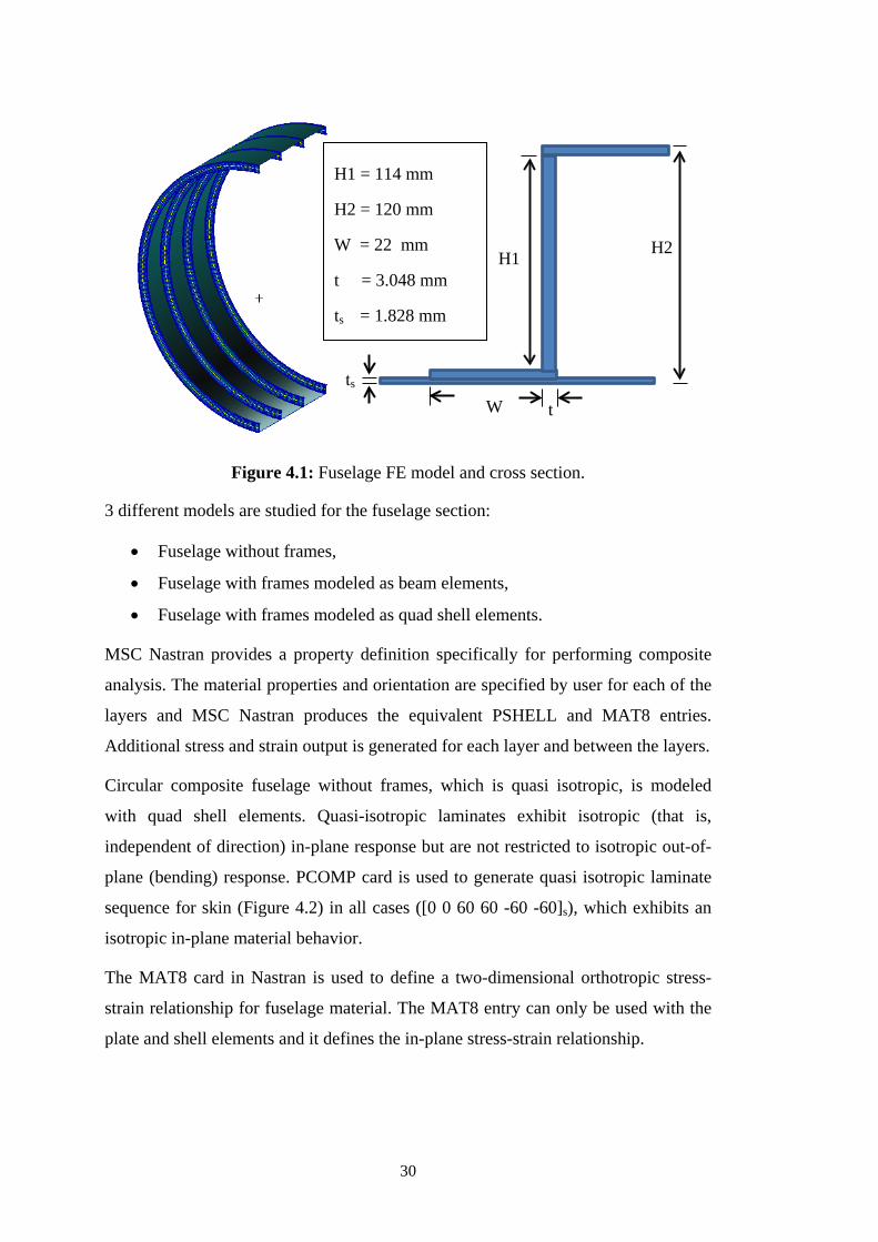
Figure 4.1: Fuselage FE model and cross section.
3 different models are studied for the fuselage section:
• Fuselage without frames,
• Fuselage with frames modeled as beam elements,
• Fuselage with frames modeled as quad shell elements.
MSC Nastran provides a property definition specifically for performing composite
analysis. The material properties and orientation are specified by user for each of the
layers and MSC Nastran produces the equivalent PSHELL and MAT8 entries.
Additional stress and strain output is generated for each layer and between the layers.
Circular composite fuselage without frames, which is quasi isotropic, is modeled
with quad shell elements. Quasi-isotropic laminates exhibit isotropic (that is,
independent of direction) in-plane response but are not restricted to isotropic out-of-
plane (bending) response. PCOMP card is used to generate quasi isotropic laminate
sequence for skin (Figure 4.2) in all cases ([0 0 60 60 -60 -60]s), which exhibits an
isotropic in-plane material behavior.
The MAT8 card in Nastran is used to define a two-dimensional orthotropic stress-
strain relationship for fuselage material. The MAT8 entry can only be used with the
plate and shell elements and it defines the in-plane stress-strain relationship.
H1 H2
t W ts
H1 = 114 mm
H2 = 120 mm
W = 22 mm
t = 3.048 mm
ts = 1.828 mm
30
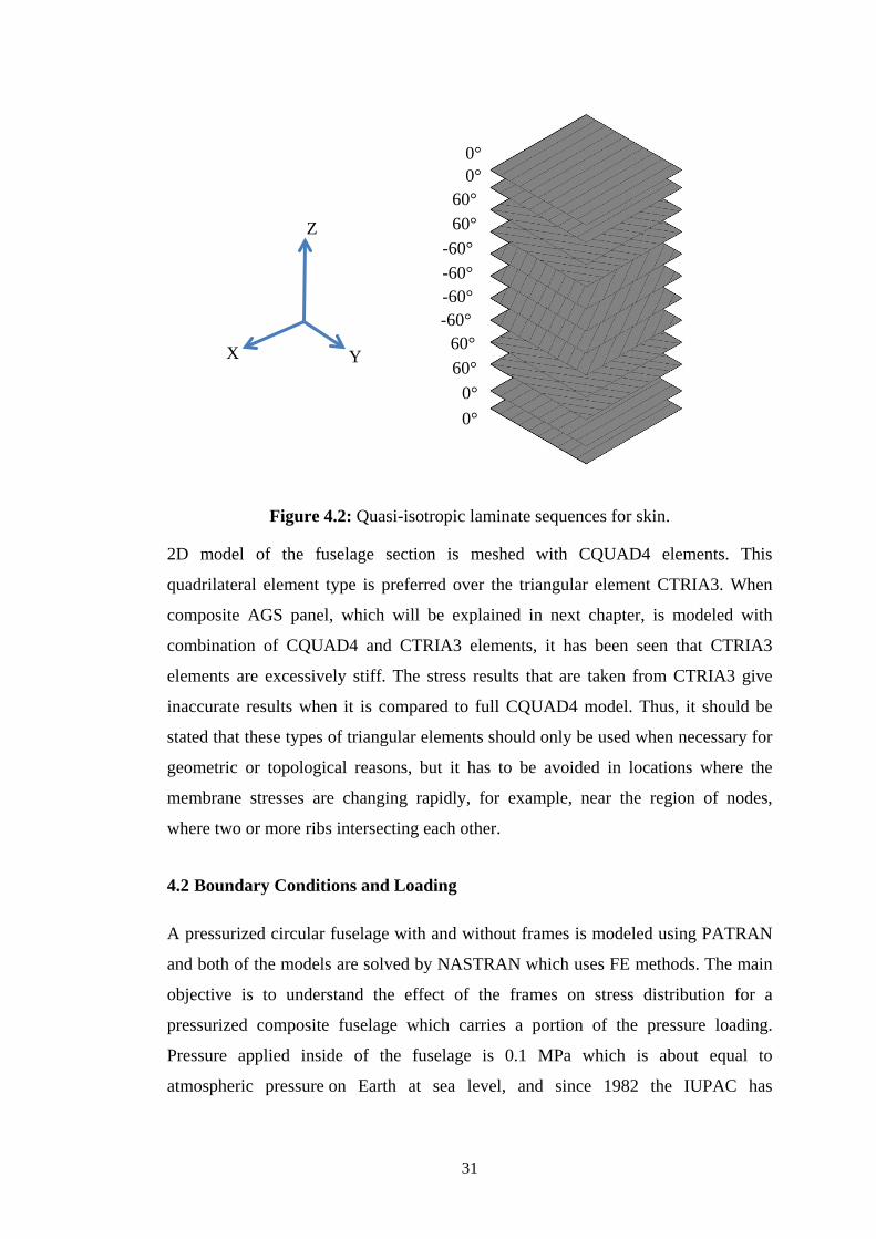
Figure 4.2: Quasi-isotropic laminate sequences for skin.
2D model of the fuselage section is meshed with CQUAD4 elements. This
quadrilateral element type is preferred over the triangular element CTRIA3. When
composite AGS panel, which will be explained in next chapter, is modeled with
combination of CQUAD4 and CTRIA3 elements, it has been seen that CTRIA3
elements are excessively stiff. The stress results that are taken from CTRIA3 give
inaccurate results when it is compared to full CQUAD4 model. Thus, it should be
stated that these types of triangular elements should only be used when necessary for
geometric or topological reasons, but it has to be avoided in locations where the
membrane stresses are changing rapidly, for example, near the region of nodes,
where two or more ribs intersecting each other.
4.2 Boundary Conditions and Loading
A pressurized circular fuselage with and without frames is modeled using PATRAN
and both of the models are solved by NASTRAN which uses FE methods. The main
objective is to understand the effect of the frames on stress distribution for a
pressurized composite fuselage which carries a portion of the pressure loading.
Pressure applied inside of the fuselage is 0.1 MPa which is about equal to
atmospheric pressure on Earth at sea level, and since 1982 the IUPAC has
0° 0°
60° 60°
-60° -60° -60° -60°
60° 60°
0° 0°
X Y
Z
31
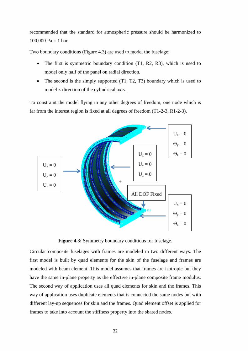
recommended that the standard for atmospheric pressure should be harmonized to
100,000 Pa = 1 bar.
Two boundary conditions (Figure 4.3) are used to model the fuselage:
• The first is symmetric boundary condition (T1, R2, R3), which is used to
model only half of the panel on radial direction,
• The second is the simply supported (T1, T2, T3) boundary which is used to
model z-direction of the cylindrical axis.
To constraint the model flying in any other degrees of freedom, one node which is
far from the interest region is fixed at all degrees of freedom (T1-2-3, R1-2-3).
Figure 4.3: Symmetry boundary conditions for fuselage.
Circular composite fuselages with frames are modeled in two different ways. The
first model is built by quad elements for the skin of the fuselage and frames are
modeled with beam element. This model assumes that frames are isotropic but they
have the same in-plane property as the effective in-plane composite frame modulus.
The second way of application uses all quad elements for skin and the frames. This
way of application uses duplicate elements that is connected the same nodes but with
different lay-up sequences for skin and the frames. Quad element offset is applied for
frames to take into account the stiffness property into the shared nodes.
Ux = 0
Uy = 0
Uz = 0
Ux = 0
Uy = 0
Uz = 0
Ux = 0
ϴy = 0
ϴz = 0
Ux = 0
ϴy = 0
ϴz = 0
All DOF Fixed
32
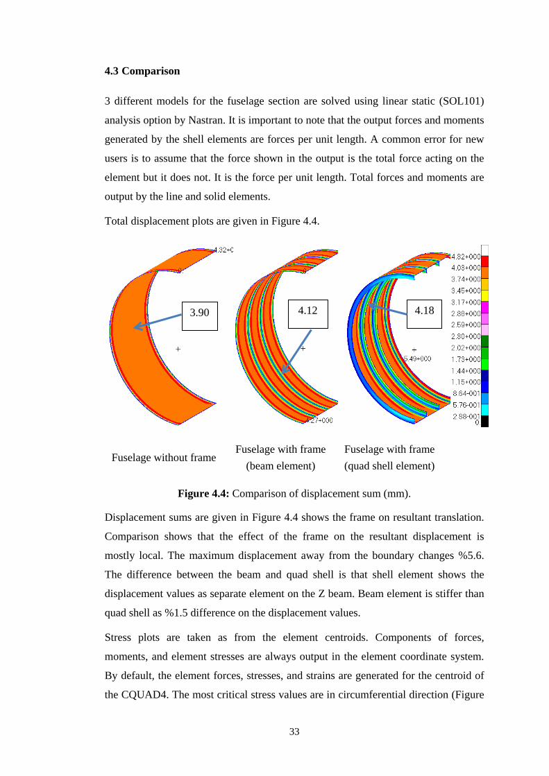
4.3 Comparison
3 different models for the fuselage section are solved using linear static (SOL101)
analysis option by Nastran. It is important to note that the output forces and moments
generated by the shell elements are forces per unit length. A common error for new
users is to assume that the force shown in the output is the total force acting on the
element but it does not. It is the force per unit length. Total forces and moments are
output by the line and solid elements.
Total displacement plots are given in Figure 4.4.
Figure 4.4: Comparison of displacement sum (mm).
Displacement sums are given in Figure 4.4 shows the frame on resultant translation.
Comparison shows that the effect of the frame on the resultant displacement is
mostly local. The maximum displacement away from the boundary changes %5.6.
The difference between the beam and quad shell is that shell element shows the
displacement values as separate element on the Z beam. Beam element is stiffer than
quad shell as %1.5 difference on the displacement values.
Stress plots are taken as from the element centroids. Components of forces,
moments, and element stresses are always output in the element coordinate system.
By default, the element forces, stresses, and strains are generated for the centroid of
the CQUAD4. The most critical stress values are in circumferential direction (Figure
Fuselage without frame Fuselage with frame
(beam element) Fuselage with frame (quad shell element)
3.90 4.12 4.18
33
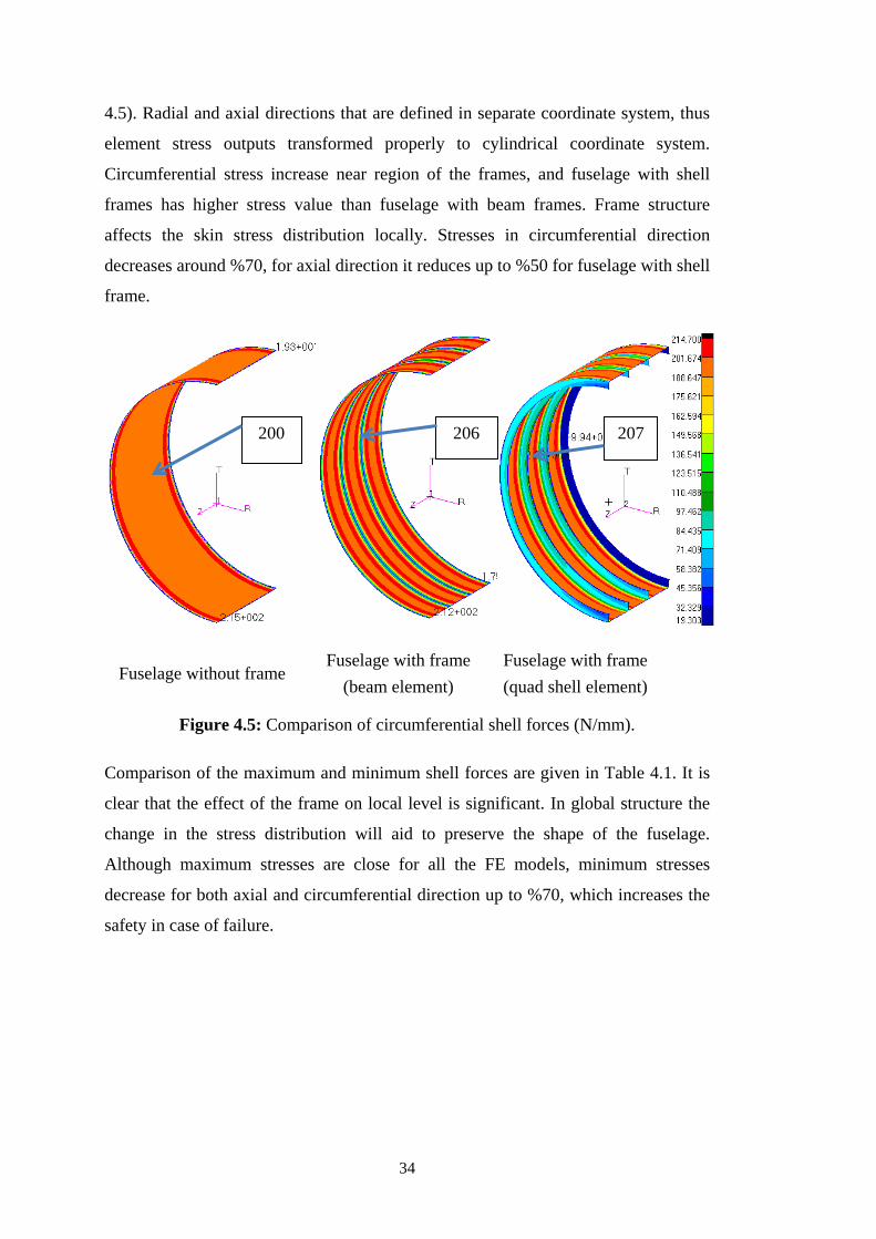
4.5). Radial and axial directions that are defined in separate coordinate system, thus
element stress outputs transformed properly to cylindrical coordinate system.
Circumferential stress increase near region of the frames, and fuselage with shell
frames has higher stress value than fuselage with beam frames. Frame structure
affects the skin stress distribution locally. Stresses in circumferential direction
decreases around %70, for axial direction it reduces up to %50 for fuselage with shell
frame.
Figure 4.5: Comparison of circumferential shell forces (N/mm).
Comparison of the maximum and minimum shell forces are given in Table 4.1. It is
clear that the effect of the frame on local level is significant. In global structure the
change in the stress distribution will aid to preserve the shape of the fuselage.
Although maximum stresses are close for all the FE models, minimum stresses
decrease for both axial and circumferential direction up to %70, which increases the
safety in case of failure.
Fuselage without frame Fuselage with frame
(beam element) Fuselage with frame (quad shell element)
200 206 207
34
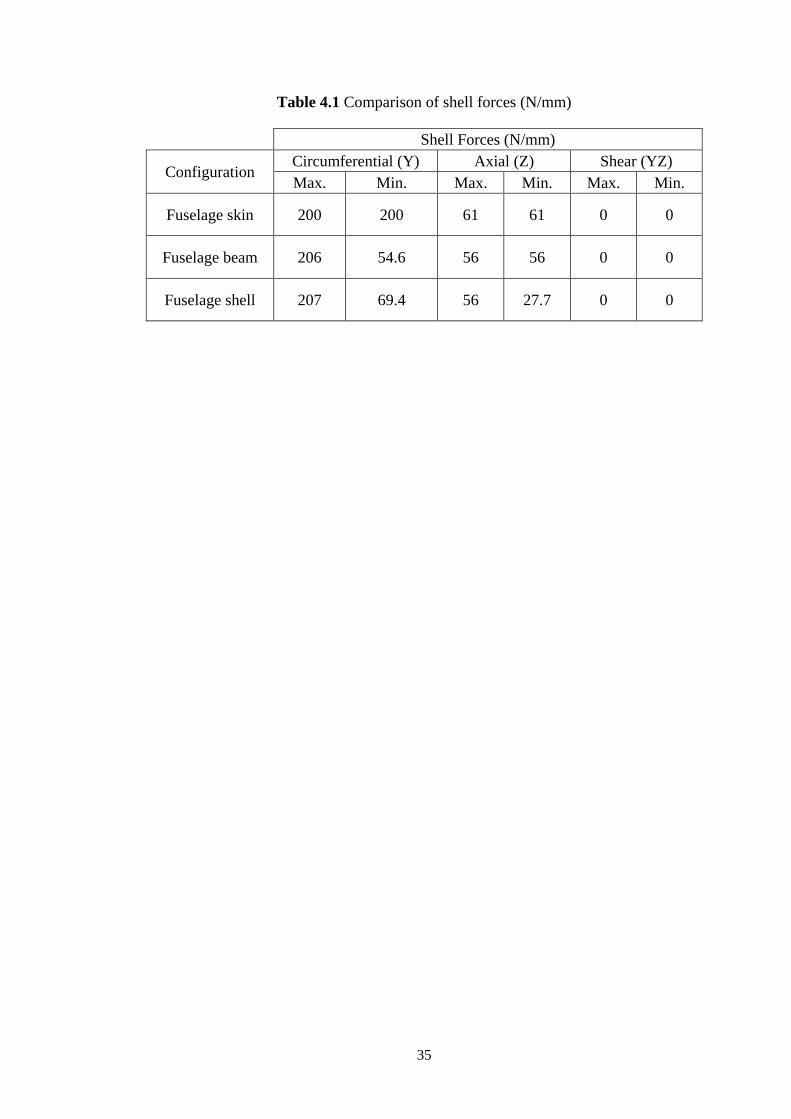
Table 4.1 Comparison of shell forces (N/mm)
Shell Forces (N/mm)
Configuration Circumferential (Y) Axial (Z) Shear (YZ) Max. Min. Max. Min. Max. Min.
Fuselage skin 200 200 61 61 0 0
Fuselage beam 206 54.6 56 56 0 0
Fuselage shell 207 69.4 56 27.7 0 0
35

36
5. FINITE ELEMENT ANALYSIS OF THE COMPOSITE AGS PANEL
In this chapter, the composite AGS panel is analyzed in detail for different type of critical loading conditions. The main analysis is done for Load Case 2, which is the optimum design model given in Chapter 6. Stress analysis plots for all the grids are given for different angles, thus maximum stresses are shown on FE model. Inter-laminar stresses are also studied for aforementioned load case. Additionally buckling modes are shown for 10 modes for the optimum model.
5.1 Modeling
There are several types of plane elements exist in commercial FE Analysis programs.
In our case, the compatible element type and a tool, which composite materials can
be defined, was the selection criteria for FEA program. Most of the conventional
FEA programs store and uses data on the basis of laminate materials. On structural
parts, this type of representation makes model extremely complicated and layers
becomes overlapping. MSC. Patran store the data of the structure in terms of its
constituent layers which makes the model easy to check and understand. Patran as a
pre-processor has a composite tool (Figure A.3) which can be used to create
orthotropic properties for laminae and composite laminate.
The input cards used to model 2D composite AGS panel consist of FE element and
material property definitions. The element library for 2D shell modelling provides
CQUAD4 element in Nastran, which defines an iso-parametric membrane-bending
or plane strain quadrilateral plate element. The properties of the n-ply composite
material laminate are defined with PCOMP card and then translated to MAT8, which
defines the material property for an orthotropic material for iso-parametric shell
elements.
Furthermore, the main idea for modeling of the composite AGS panel is using
quadrilateral elements or quadrilateral elements mixed with triangular elements,
where it is impossible to mesh with quadrilateral elements. As it is given in literature
study chapter, researchers tried different types of elements which can cover the
37
behavior of composite AGS panel as a skin and stiffener, but the main purpose of
this thesis is to define a model using existing FEA 2D quadrilateral element types
that can simulate the behavior of the surface and stiffeners of the composite AGS
panel.
Correspondingly, the following decision is about how to input the stiffness
parameters into the nodes representing the AGS plate. As it is known, FEA programs
uses elements to make connection between nodes. In our case, this connection could
be possible in three ways using 2D quadrilateral elements;
• The first way is to model stiffeners as separate quadrilateral elements that one
edge nodes are connected to the nodes of the surface and to model surface
elements, mesh should follow the stiffener geometry. Disadvantage of this
type of modeling is thickness of the stiffeners is actually not modeled
physically. Thus, global model geometry is altered and accuracy of global
and local buckling analysis is lost.
• The second way is to model a geometry which stiffeners are also modeled as
2D projection on x-y plane, by the aid of the layer based modeling, the
stiffener geometry would include the surface and stiffener layers altogether
through the lattice geometry. It gives better accuracy for the buckling modes
of the AGS panel but continuity on skin layers and the stiffener layers are
lost.
• The third one, which is found suitable for our model, is to model stiffener and
the surface as separate elements, and the pattern of the mesh should follow
the lattice of the AGS plate. This application uses duplicate elements
approach. The most important advantage of this type of definition of the AGS
panel, an engineer is able to model physical body with exact geometry
without losing any stiffness parameters. Therefore, optimization or especially
the local and global buckling analysis of the same structure can be conducted
without losing the accuracy and the insight of the quadrilateral element
behavior.
5.2 Meshing
There are two types of elements available to model 2D panel. CQUAD4 and
CTRIA3 elements can be used separately or together as described below. All
38
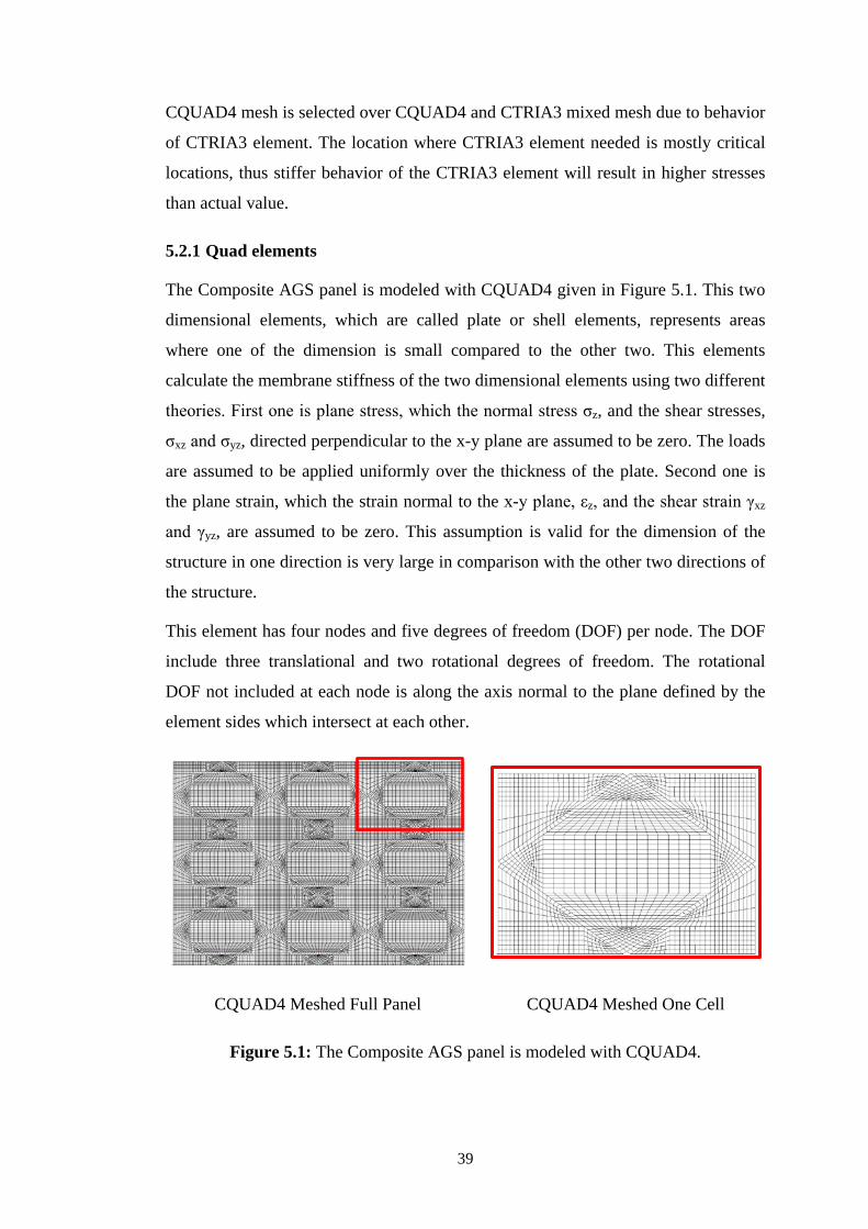
CQUAD4 mesh is selected over CQUAD4 and CTRIA3 mixed mesh due to behavior
of CTRIA3 element. The location where CTRIA3 element needed is mostly critical
locations, thus stiffer behavior of the CTRIA3 element will result in higher stresses
than actual value.
5.2.1 Quad elements
The Composite AGS panel is modeled with CQUAD4 given in Figure 5.1. This two
dimensional elements, which are called plate or shell elements, represents areas
where one of the dimension is small compared to the other two. This elements
calculate the membrane stiffness of the two dimensional elements using two different
theories. First one is plane stress, which the normal stress σz, and the shear stresses,
σxz and σyz, directed perpendicular to the x-y plane are assumed to be zero. The loads
are assumed to be applied uniformly over the thickness of the plate. Second one is
the plane strain, which the strain normal to the x-y plane, εz, and the shear strain γxz
and γyz, are assumed to be zero. This assumption is valid for the dimension of the
structure in one direction is very large in comparison with the other two directions of
the structure.
This element has four nodes and five degrees of freedom (DOF) per node. The DOF
include three translational and two rotational degrees of freedom. The rotational
DOF not included at each node is along the axis normal to the plane defined by the
element sides which intersect at each other.
Figure 5.1: The Composite AGS panel is modeled with CQUAD4.
CQUAD4 Meshed Full Panel CQUAD4 Meshed One Cell
39
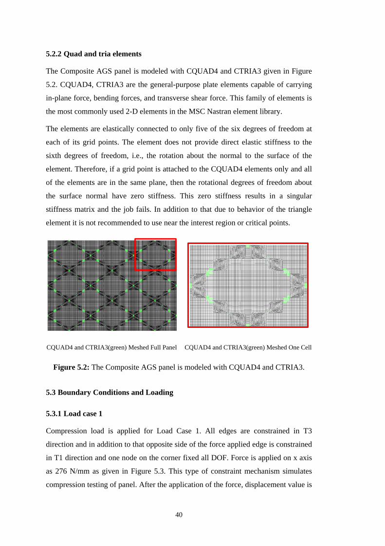
5.2.2 Quad and tria elements
The Composite AGS panel is modeled with CQUAD4 and CTRIA3 given in Figure
5.2. CQUAD4, CTRIA3 are the general-purpose plate elements capable of carrying
in-plane force, bending forces, and transverse shear force. This family of elements is
the most commonly used 2-D elements in the MSC Nastran element library.
The elements are elastically connected to only five of the six degrees of freedom at
each of its grid points. The element does not provide direct elastic stiffness to the
sixth degrees of freedom, i.e., the rotation about the normal to the surface of the
element. Therefore, if a grid point is attached to the CQUAD4 elements only and all
of the elements are in the same plane, then the rotational degrees of freedom about
the surface normal have zero stiffness. This zero stiffness results in a singular
stiffness matrix and the job fails. In addition to that due to behavior of the triangle
element it is not recommended to use near the interest region or critical points.
Figure 5.2: The Composite AGS panel is modeled with CQUAD4 and CTRIA3.
5.3 Boundary Conditions and Loading
5.3.1 Load case 1
Compression load is applied for Load Case 1. All edges are constrained in T3
direction and in addition to that opposite side of the force applied edge is constrained
in T1 direction and one node on the corner fixed all DOF. Force is applied on x axis
as 276 N/mm as given in Figure 5.3. This type of constraint mechanism simulates
compression testing of panel. After the application of the force, displacement value is
CQUAD4 and CTRIA3(green) Meshed Full Panel CQUAD4 and CTRIA3(green) Meshed One Cell
40
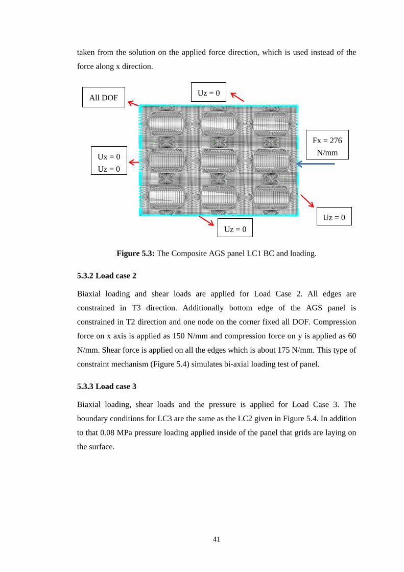
taken from the solution on the applied force direction, which is used instead of the
force along x direction.
Figure 5.3: The Composite AGS panel LC1 BC and loading.
5.3.2 Load case 2
Biaxial loading and shear loads are applied for Load Case 2. All edges are
constrained in T3 direction. Additionally bottom edge of the AGS panel is
constrained in T2 direction and one node on the corner fixed all DOF. Compression
force on x axis is applied as 150 N/mm and compression force on y is applied as 60
N/mm. Shear force is applied on all the edges which is about 175 N/mm. This type of
constraint mechanism (Figure 5.4) simulates bi-axial loading test of panel.
5.3.3 Load case 3
Biaxial loading, shear loads and the pressure is applied for Load Case 3. The
boundary conditions for LC3 are the same as the LC2 given in Figure 5.4. In addition
to that 0.08 MPa pressure loading applied inside of the panel that grids are laying on
the surface.
Uz = 0
Ux = 0 Uz = 0
Fx = 276 N/mm
Uz = 0 Uz = 0
All DOF
41
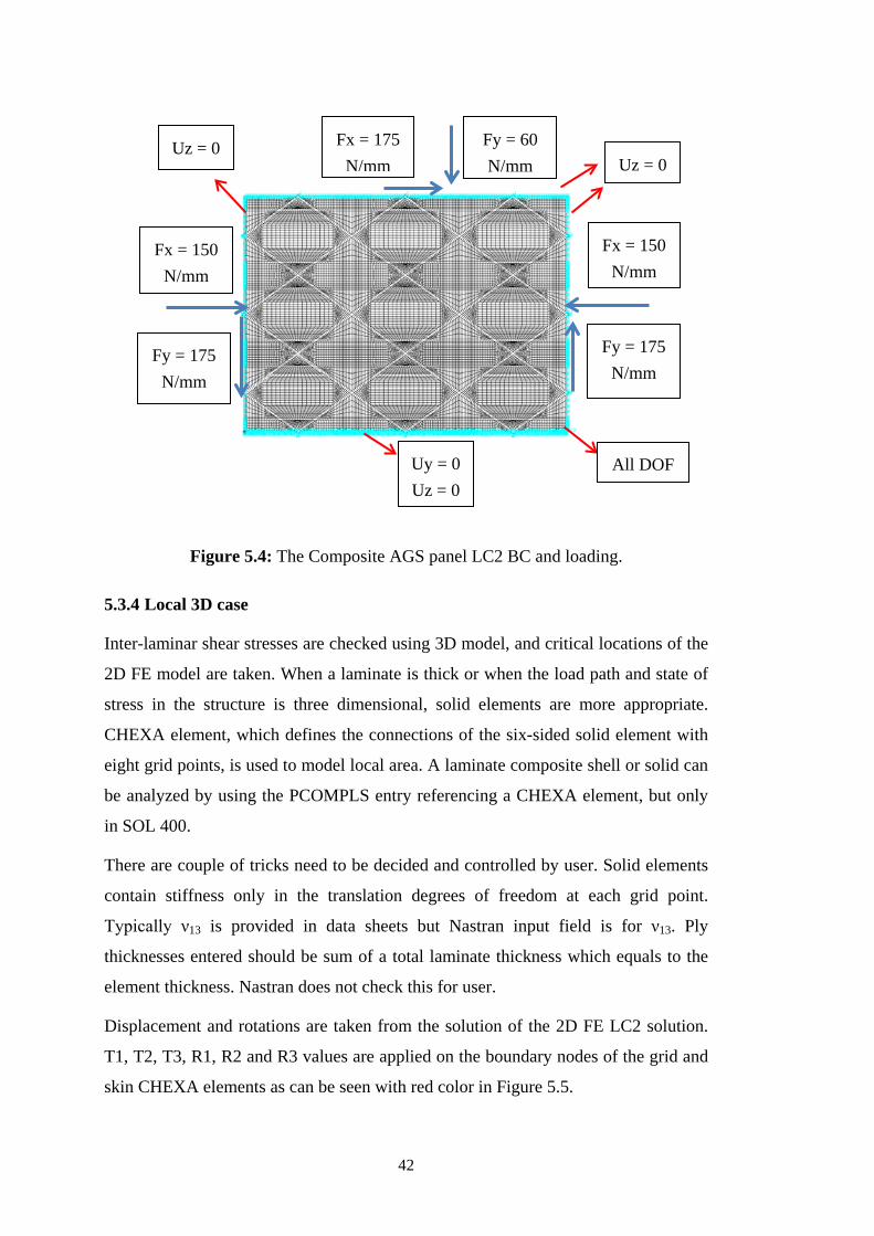
Figure 5.4: The Composite AGS panel LC2 BC and loading.
5.3.4 Local 3D case
Inter-laminar shear stresses are checked using 3D model, and critical locations of the
2D FE model are taken. When a laminate is thick or when the load path and state of
stress in the structure is three dimensional, solid elements are more appropriate.
CHEXA element, which defines the connections of the six-sided solid element with
eight grid points, is used to model local area. A laminate composite shell or solid can
be analyzed by using the PCOMPLS entry referencing a CHEXA element, but only
in SOL 400.
There are couple of tricks need to be decided and controlled by user. Solid elements
contain stiffness only in the translation degrees of freedom at each grid point.
Typically ν13 is provided in data sheets but Nastran input field is for ν13. Ply
thicknesses entered should be sum of a total laminate thickness which equals to the
element thickness. Nastran does not check this for user.
Displacement and rotations are taken from the solution of the 2D FE LC2 solution.
T1, T2, T3, R1, R2 and R3 values are applied on the boundary nodes of the grid and
skin CHEXA elements as can be seen with red color in Figure 5.5.
Fx = 150 N/mm
Uy = 0 Uz = 0
All DOF
Fy = 175 N/mm
Fx = 150 N/mm
Fy = 175 N/mm
Uz = 0 Fy = 60 N/mm
Fx = 175 N/mm
Uz = 0
42
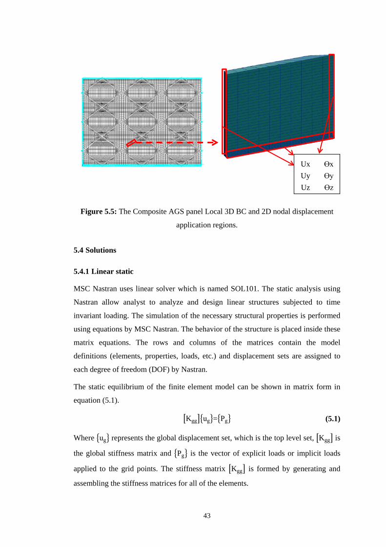
Figure 5.5: The Composite AGS panel Local 3D BC and 2D nodal displacement
application regions.
5.4 Solutions
5.4.1 Linear static
MSC Nastran uses linear solver which is named SOL101. The static analysis using
Nastran allow analyst to analyze and design linear structures subjected to time
invariant loading. The simulation of the necessary structural properties is performed
using equations by MSC Nastran. The behavior of the structure is placed inside these
matrix equations. The rows and columns of the matrices contain the model
definitions (elements, properties, loads, etc.) and displacement sets are assigned to
each degree of freedom (DOF) by Nastran.
The static equilibrium of the finite element model can be shown in matrix form in
equation (5.1).
Where �ug� represents the global displacement set, which is the top level set, �Kgg� is
the global stiffness matrix and �Pg� is the vector of explicit loads or implicit loads
applied to the grid points. The stiffness matrix �Kgg� is formed by generating and
assembling the stiffness matrices for all of the elements.
�Kgg��ug�=�Pg� (5.1)
Ux ϴx Uy ϴy Uz ϴz
43
For linear analysis, MSC Nastran plate elements assume classical engineering
assumptions of thin plate behavior,
• The deflection of the mid-surface is small compared with the thickness
• The mid-surface remains unstrained (neutral) during bending. (This applies to
lateral loads, not in-plane loads.)
• The normal to the mid-surface remains normal to the mid-surface during
bending
5.4.2 Buckling
MSC Nastran uses linear solver which is named SOL105. Global and local instability
modes of composite AGS panel are analyzed using Nastran solver. The buckling
solution of the plate is assumed to be in linear range so that yielding of the structure
and change of force direction are not included in the solution.
Linear buckling analysis using finite elements defines two stiffness properties which
are differential stiffness and linear stiffness. The difference between two of them is
differential stiffness that is constructed from higher-order terms of the strain-
displacement relationships. The question comes into mind when instability behavior
of the structure occurs, how can the compressive and tensile axial loading affect the
linear stiffness matrix? Thus, differential stiffness matrix represents the linear
approximation of softening (reducing) the linear stiffness matrix in the case of
compressive axial load, and stiffening (increasing) the linear stiffness matrix in the
case of a tensile axial load. The element stiffness matrices are denoted as below in
equation (5.2).
The differential stiffness is a function of the geometry, element type, and applied
load. The global linear stiffness matrix can be represented as equation (5.3).
[ka]i = linear stiffness matrix
[kd]i = differential stiffness matrix (5.2)
[Ka]=� kai
n
i
(5.3)
44
As linear stiffness matrix, the global differential stiffness matrix can be represented
as equation (5.4).
The overall system stiffness matrix is represented as equation (5.5).
Total potential of the system must have stationary value to achieve static equilibrium,
a can be given in formulation (5.6).
where ui is the displacement of the ith degree of freedom.
Finite element model has finite number of degrees of freedom, although structures
have infinite number of degrees of freedom in the real world. The number of
buckling approximation of the structural behavior is proportional with the number of
degrees of freedom of our model. It is formulated as in equation (5.7).
Thus it gives the equation 5.8,
The above form of problems is called as eigenvalue problem. Once 𝜆𝑖 values are
obtained, the buckling load can be calculated using equation (5.7). In addition to that
𝜆𝑖 values are the scale factors by which the applied load Pais multiplied to generate
the critical buckling loads Pcri.
In general, only the first two or three buckling loads are of any practical interest. The
structure will fail prior to reaching any of the higher buckling loads other than first
buckling load. MSC Nastran can perform buckling analysis on any or all of the
loading conditions but it should be noted that it is valid for small deflections and
elastic range. If it is an axial loading condition, applied load can be multiplied by the
eigenvalue to obtain the buckling load.
[Kd]=� kdi
n
i
(5.4)
[K]=[Ka]+[Kd] (5.5)
∂[U]∂ui
=[Ka]{u}+[Kd]{u}={0} (5.6)
Pcri=λi Pa (5.7)
|[Ka]+λi[Kd]|=[0] (5.8)
45
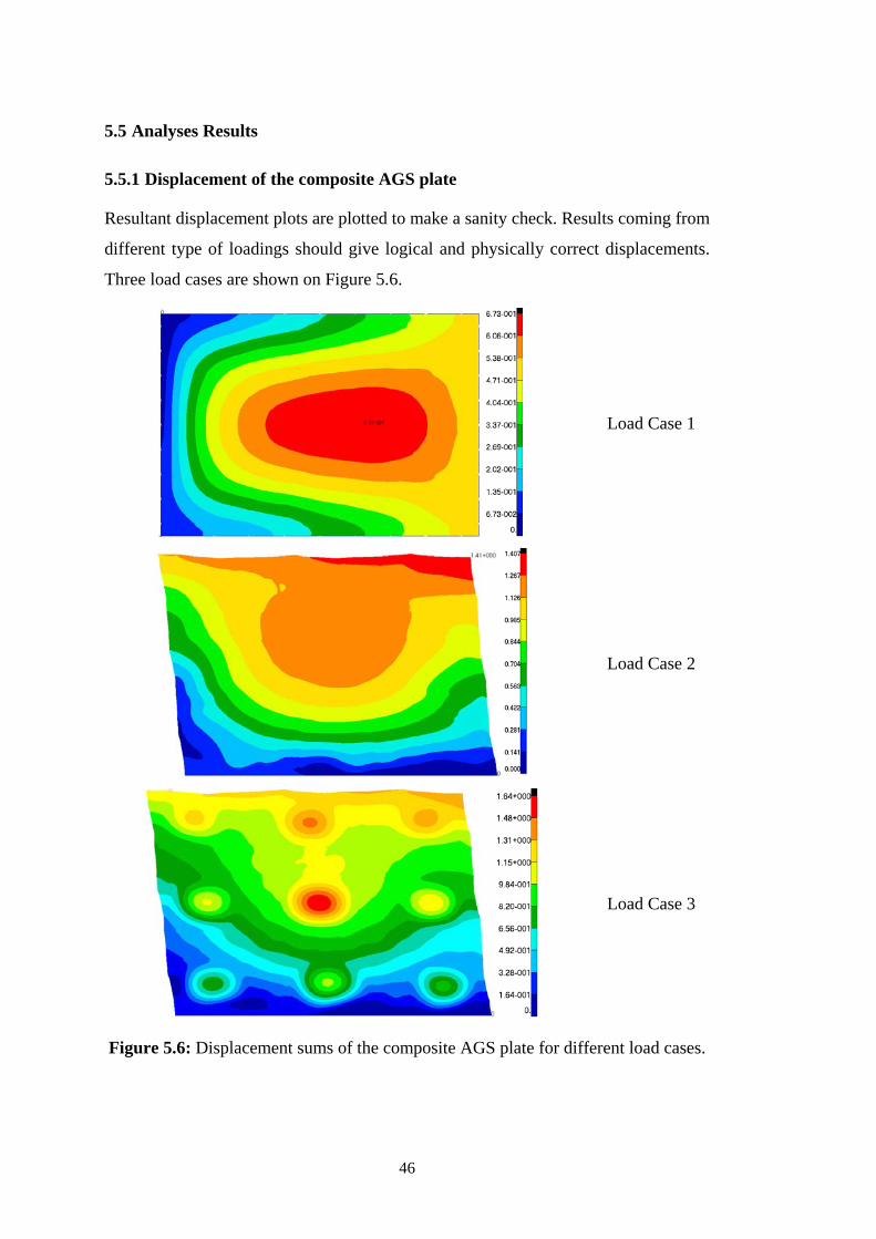
5.5 Analyses Results
5.5.1 Displacement of the composite AGS plate
Resultant displacement plots are plotted to make a sanity check. Results coming from
different type of loadings should give logical and physically correct displacements.
Three load cases are shown on Figure 5.6.
Figure 5.6: Displacement sums of the composite AGS plate for different load cases.
Load Case 1
Load Case 2
Load Case 3
46
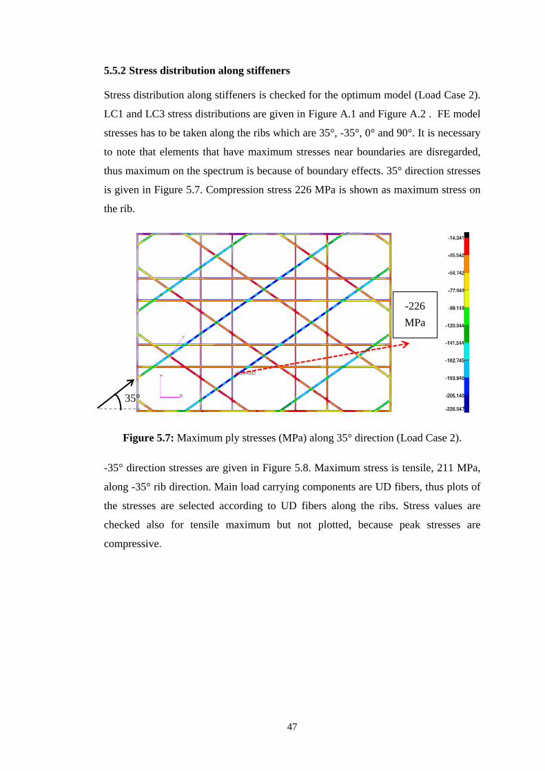
5.5.2 Stress distribution along stiffeners
Stress distribution along stiffeners is checked for the optimum model (Load Case 2).
LC1 and LC3 stress distributions are given in Figure A.1 and Figure A.2 . FE model
stresses has to be taken along the ribs which are 35°, -35°, 0° and 90°. It is necessary
to note that elements that have maximum stresses near boundaries are disregarded,
thus maximum on the spectrum is because of boundary effects. 35° direction stresses
is given in Figure 5.7. Compression stress 226 MPa is shown as maximum stress on
the rib.
Figure 5.7: Maximum ply stresses (MPa) along 35° direction (Load Case 2).
-35° direction stresses are given in Figure 5.8. Maximum stress is tensile, 211 MPa,
along -35° rib direction. Main load carrying components are UD fibers, thus plots of
the stresses are selected according to UD fibers along the ribs. Stress values are
checked also for tensile maximum but not plotted, because peak stresses are
compressive.
-226 MPa
35°
47
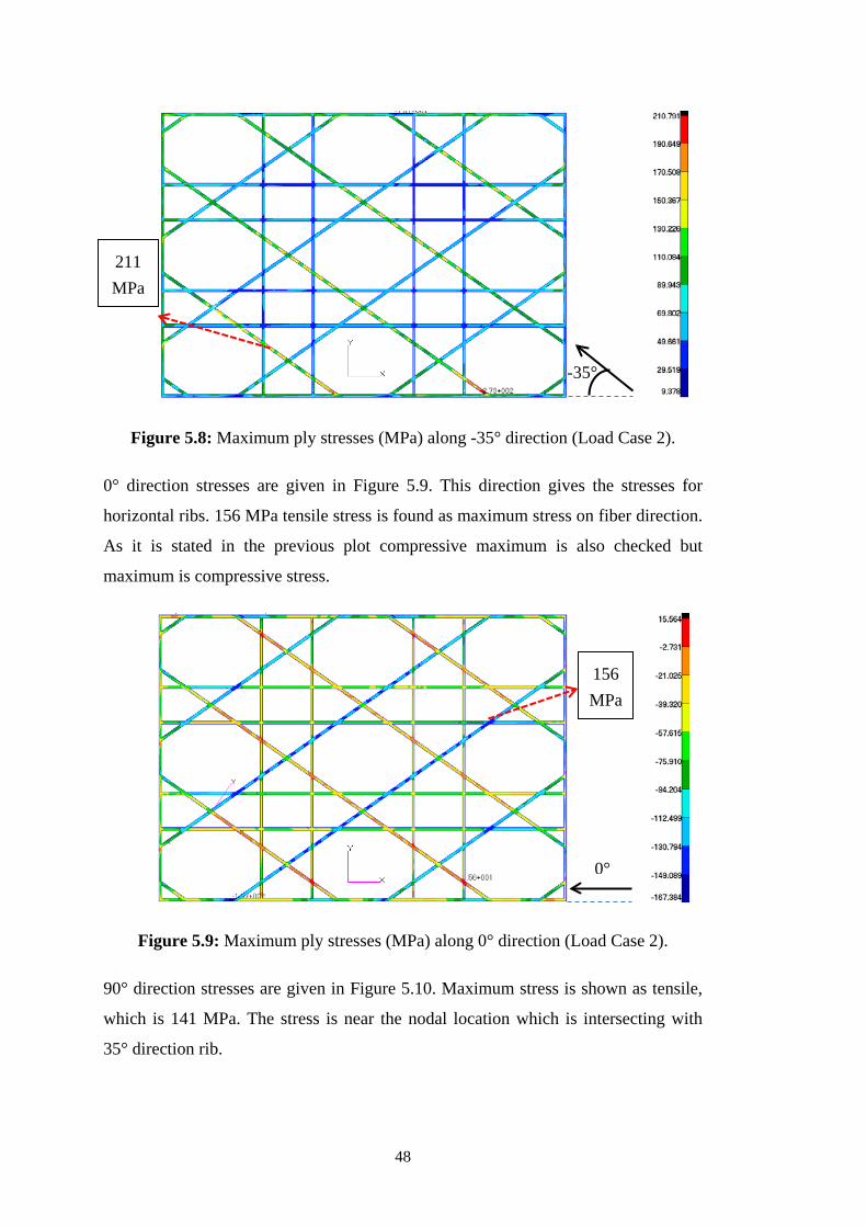
Figure 5.8: Maximum ply stresses (MPa) along -35° direction (Load Case 2).
0° direction stresses are given in Figure 5.9. This direction gives the stresses for
horizontal ribs. 156 MPa tensile stress is found as maximum stress on fiber direction.
As it is stated in the previous plot compressive maximum is also checked but
maximum is compressive stress.
Figure 5.9: Maximum ply stresses (MPa) along 0° direction (Load Case 2).
90° direction stresses are given in Figure 5.10. Maximum stress is shown as tensile,
which is 141 MPa. The stress is near the nodal location which is intersecting with
35° direction rib.
211 MPa
-35°
156 MPa
0°
48
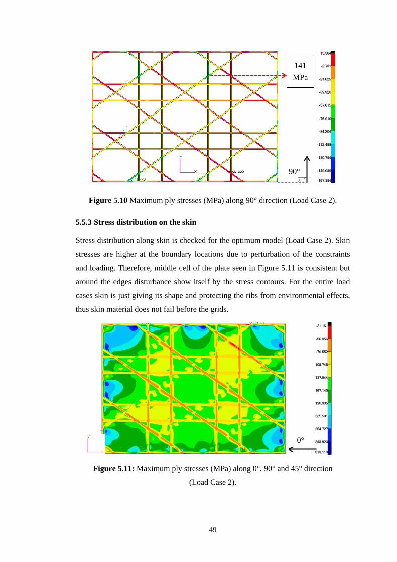
Figure 5.10 Maximum ply stresses (MPa) along 90° direction (Load Case 2).
5.5.3 Stress distribution on the skin
Stress distribution along skin is checked for the optimum model (Load Case 2). Skin
stresses are higher at the boundary locations due to perturbation of the constraints
and loading. Therefore, middle cell of the plate seen in Figure 5.11 is consistent but
around the edges disturbance show itself by the stress contours. For the entire load
cases skin is just giving its shape and protecting the ribs from environmental effects,
thus skin material does not fail before the grids.
Figure 5.11: Maximum ply stresses (MPa) along 0°, 90° and 45° direction
(Load Case 2).
90°
141 MPa
0°
49
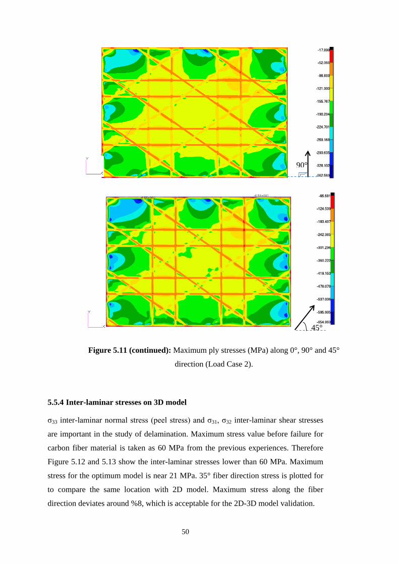
5.5.4 Inter-laminar stresses on 3D model
σ33 inter-laminar normal stress (peel stress) and σ31, σ32 inter-laminar shear stresses
are important in the study of delamination. Maximum stress value before failure for
carbon fiber material is taken as 60 MPa from the previous experiences. Therefore
Figure 5.12 and 5.13 show the inter-laminar stresses lower than 60 MPa. Maximum
stress for the optimum model is near 21 MPa. 35° fiber direction stress is plotted for
to compare the same location with 2D model. Maximum stress along the fiber
direction deviates around %8, which is acceptable for the 2D-3D model validation.
Figure 5.11 (continued): Maximum ply stresses (MPa) along 0°, 90° and 45°
direction (Load Case 2).
90°
45°
50
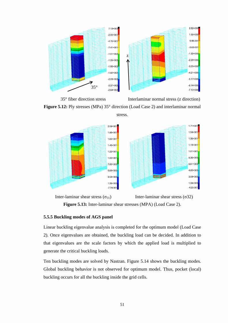
Figure 5.12: Ply stresses (MPa) 35° direction (Load Case 2) and interlaminar normal
stress.
Figure 5.13: Inter-laminar shear stresses (MPA) (Load Case 2).
5.5.5 Buckling modes of AGS panel
Linear buckling eigenvalue analysis is completed for the optimum model (Load Case
2). Once eigenvalues are obtained, the buckling load can be decided. In addition to
that eigenvalues are the scale factors by which the applied load is multiplied to
generate the critical buckling loads.
Ten buckling modes are solved by Nastran. Figure 5.14 shows the buckling modes.
Global buckling behavior is not observed for optimum model. Thus, pocket (local)
buckling occurs for all the buckling inside the grid cells.
35° fiber direction stress Interlaminar normal stress (z direction)
Inter-laminar shear stress (σ31) Inter-laminar shear stress (σ32)
35°
z
51
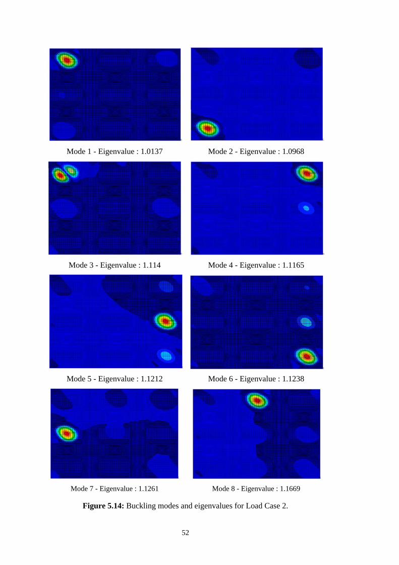
Mode 1 - Eigenvalue : 1.0137 Mode 2 - Eigenvalue : 1.0968
Mode 3 - Eigenvalue : 1.114 Mode 4 - Eigenvalue : 1.1165
Mode 5 - Eigenvalue : 1.1212 Mode 6 - Eigenvalue : 1.1238
Mode 7 - Eigenvalue : 1.1261 Mode 8 - Eigenvalue : 1.1669
Figure 5.14: Buckling modes and eigenvalues for Load Case 2.
52
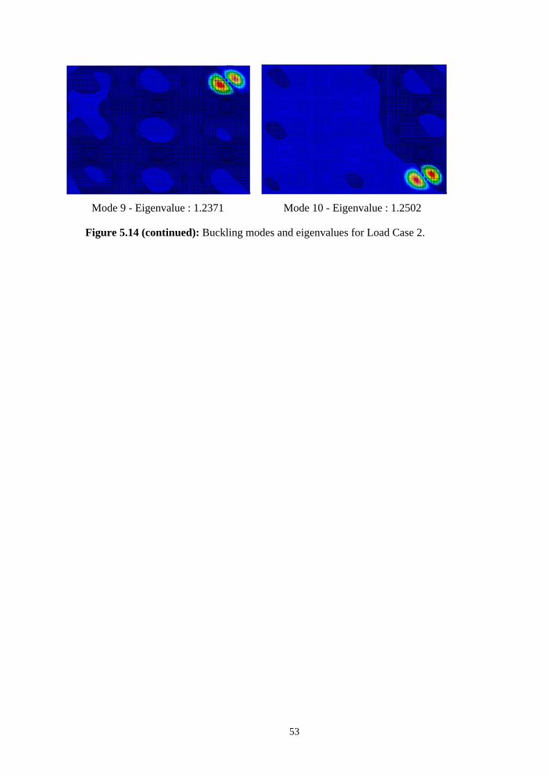
Mode 9 - Eigenvalue : 1.2371 Mode 10 - Eigenvalue : 1.2502
Figure 5.14 (continued): Buckling modes and eigenvalues for Load Case 2.
53

54
6. FINITE ELEMENT OPTIMISATION OF AGS PANEL
This chapter elaborates on the FE optimizations performed as part of the thesis project. As given in Chapter 5, Load Case 2 with the aforementioned boundary condition is used to create design model for panel optimization. Several optimizations were carried out for different configurations of the composite AGS panel.
6.1 Msc Nastran Optimization – How it works?
The composite AGS structure is improved through a design process by using MSC
Nastran. Design optimization process searches for optimal or “the best” structural
parameters and the searching operation uses some mathematical approaches to yield
improved design.
An important concept of optimization is design sensitivity analysis, which gives the
connection between the change of structural responses and changes in design
parameters. These design variables or parameters can be anything depending upon
analysis objective which is thickness, width of stiffeners and dimension of one cell
lattice pattern for our case. These parameters affect the material failure behavior and
buckling conditions, thus the rate of change is called design sensitivity coefficients.
This sensitivity approach is the main information to perform optimization by MSC
Nastran. Therefore, the current state of the optimized design is understood by using
FE Model results and sensitivity gives an idea which way to look for an improved
design. This algorithm is very useful especially for two or more design variables
included in the optimization due to increasing number of possible solutions
(analyses).
There are idealized statements to construct a design model:
• Design objective is the statement of what an improved means.
• Design constraint constitutes certain bounds, which the response of the
system does not exceed.
55
• Design variable (side constraints) describes how the design might be changed
and the meaning of a suitable variation.
• Design space is the definition of mathematical region over which design
variables, objective, and constraints. Design space contains the local minima,
which is the acceptable solution but can be more than one. As it is
improvement of the design model, a unique solution is the goal of
optimization.
The important thing for FEM based optimization, analysis results that are used in
each cycle of the optimization is directly connected to the constructed FE Model.
Thus, any mistake on meshed finite element model may lead to inaccurate and
misleading results.
FEM optimization user has to know some limitations. MSC Nastran uses a numerical
optimizer which is trying to find maximum or minimum depending on the objective,
which has to be defined explicitly. Design model definition will result in a bound on
responses and design variables, and this limits and objectives are directly used in the
optimization cycle.
Numerical optimization algorithms that rely on gradient information are called
“gradient based”. The basic optimization problem statement can be given as the
mathematical expression,
X needs to be found as minimum or maximum (Equation (6.1)).
which is subject to inequalities given in equation (6.2).
The objective function, which is the function of the set of design variables, needs to
be minimized. Side constraints limit the region of search and the inequality
constraints is satisfied if its value is negative by convention. Equality constraints give
the exact optimal design.
F(X) objective (6.1)
gj(X) ≤ 0 j = 1,…,ng inequality constraints
hk(X) = 0 k = 1,…,nh equality constraints
xiL ≤ xi ≤ xi
U i = 1,…,n side constraints
X = {x1,x2,…,xn} design variable
(6.2)
56
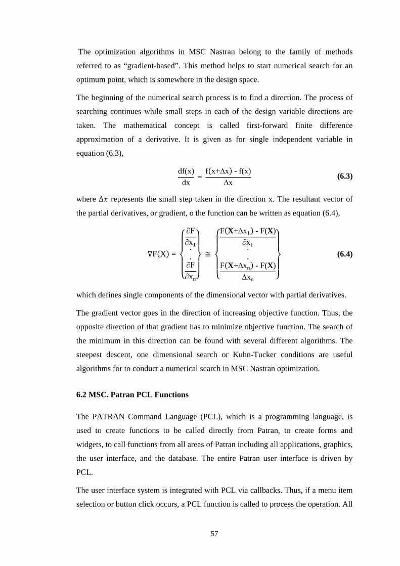
The optimization algorithms in MSC Nastran belong to the family of methods
referred to as “gradient-based”. This method helps to start numerical search for an
optimum point, which is somewhere in the design space.
The beginning of the numerical search process is to find a direction. The process of
searching continues while small steps in each of the design variable directions are
taken. The mathematical concept is called first-forward finite difference
approximation of a derivative. It is given as for single independent variable in
equation (6.3),
where ∆𝑥 represents the small step taken in the direction x. The resultant vector of
the partial derivatives, or gradient, o the function can be written as equation (6.4),
which defines single components of the dimensional vector with partial derivatives.
The gradient vector goes in the direction of increasing objective function. Thus, the
opposite direction of that gradient has to minimize objective function. The search of
the minimum in this direction can be found with several different algorithms. The
steepest descent, one dimensional search or Kuhn-Tucker conditions are useful
algorithms for to conduct a numerical search in MSC Nastran optimization.
6.2 MSC. Patran PCL Functions
The PATRAN Command Language (PCL), which is a programming language, is
used to create functions to be called directly from Patran, to create forms and
widgets, to call functions from all areas of Patran including all applications, graphics,
the user interface, and the database. The entire Patran user interface is driven by
PCL.
The user interface system is integrated with PCL via callbacks. Thus, if a menu item
selection or button click occurs, a PCL function is called to process the operation. All
df(x)dx
= f(x+∆x) - f(x)
∆x (6.3)
∇F(X) =
⎩⎪⎨
⎪⎧
∂F∂x1.
.∂F∂xn⎭
⎪⎬
⎪⎫
≅
⎩⎪⎨
⎪⎧
F(X+∆x1) - F(X)∂x1.
.F(X+∆xn) - F(X)
∆xn ⎭⎪⎬
⎪⎫
(6.4)
57
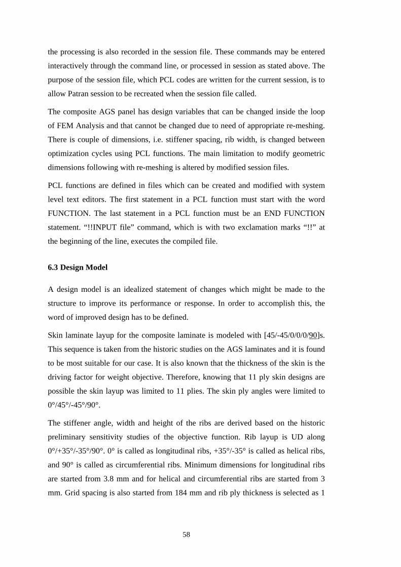
the processing is also recorded in the session file. These commands may be entered
interactively through the command line, or processed in session as stated above. The
purpose of the session file, which PCL codes are written for the current session, is to
allow Patran session to be recreated when the session file called.
The composite AGS panel has design variables that can be changed inside the loop
of FEM Analysis and that cannot be changed due to need of appropriate re-meshing.
There is couple of dimensions, i.e. stiffener spacing, rib width, is changed between
optimization cycles using PCL functions. The main limitation to modify geometric
dimensions following with re-meshing is altered by modified session files.
PCL functions are defined in files which can be created and modified with system
level text editors. The first statement in a PCL function must start with the word
FUNCTION. The last statement in a PCL function must be an END FUNCTION
statement. “!!INPUT file” command, which is with two exclamation marks “!!” at
the beginning of the line, executes the compiled file.
6.3 Design Model
A design model is an idealized statement of changes which might be made to the
structure to improve its performance or response. In order to accomplish this, the
word of improved design has to be defined.
Skin laminate layup for the composite laminate is modeled with [45/-45/0/0/0/90]s.
This sequence is taken from the historic studies on the AGS laminates and it is found
to be most suitable for our case. It is also known that the thickness of the skin is the
driving factor for weight objective. Therefore, knowing that 11 ply skin designs are
possible the skin layup was limited to 11 plies. The skin ply angles were limited to
0°/45°/-45°/90°.
The stiffener angle, width and height of the ribs are derived based on the historic
preliminary sensitivity studies of the objective function. Rib layup is UD along
0°/+35°/-35°/90°. 0° is called as longitudinal ribs, +35°/-35° is called as helical ribs,
and 90° is called as circumferential ribs. Minimum dimensions for longitudinal ribs
are started from 3.8 mm and for helical and circumferential ribs are started from 3
mm. Grid spacing is also started from 184 mm and rib ply thickness is selected as 1
58
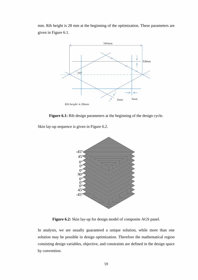
mm. Rib height is 28 mm at the beginning of the optimization. These parameters are
given in Figure 6.1.
Figure 6.1: Rib design parameters at the beginning of the design cycle.
Skin lay-up sequence is given in Figure 6.2.
Figure 6.2: Skin lay-up for design model of composite AGS panel.
In analysis, we are usually guaranteed a unique solution, while more than one
solution may be possible in design optimization. Therefore the mathematical region
consisting design variables, objective, and constraints are defined in the design space
by convention.
-45° 45° 0° 0° 0°
90°
0° 0°
0° 45°
-45°
59
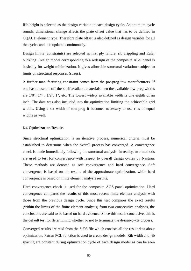
Rib height is selected as the design variable in each design cycle. As optimum cycle
rounds, dimensional change affects the plate offset value that has to be defined in
CQAUD element type. Therefore plate offset is also defined as design variable for all
the cycles and it is updated continuously.
Design limits (constraints) are selected as first ply failure, rib crippling and Euler
buckling. Design model corresponding to a redesign of the composite AGS panel is
basically for weight minimization. It gives allowable structural variations subject to
limits on structural responses (stress).
A further manufacturing constraint comes from the pre-preg tow manufacturers. If
one has to use the off-the-shelf available materials then the available tow-preg widths
are 1/8", 1/4", 1/2", 1", etc. The lowest widely available width is one eighth of an
inch. The data was also included into the optimization limiting the achievable grid
widths. Using a set width of tow-preg it becomes necessary to use ribs of equal
widths as well.
6.4 Optimization Results
Since structural optimization is an iterative process, numerical criteria must be
established to determine when the overall process has converged. A convergence
check is made immediately following the structural analysis. In reality, two methods
are used to test for convergence with respect to overall design cycles by Nastran.
These methods are denoted as soft convergence and hard convergence. Soft
convergence is based on the results of the approximate optimization, while hard
convergence is based on finite element analysis results.
Hard convergence check is used for the composite AGS panel optimization. Hard
convergence compares the results of this most recent finite element analysis with
those from the previous design cycle. Since this test compares the exact results
(within the limits of the finite element analysis) from two consecutive analyses, the
conclusions are said to be based on hard evidence. Since this test is conclusive, this is
the default test for determining whether or not to terminate the design-cycle process.
Converged results are read from the *.f06 file which consists all the result data about
optimization. Patran PCL function is used to create design models. Rib width and rib
spacing are constant during optimization cycle of each design model as can be seen
60

from Figure 6.3. Optm_3 with 205.89 mm rib spacing design model is selected as the
optimum model as shown Table 6.1 and detailed FEM analysis are conducted for it.
Weight of the panel, buckling modes under Load Case 2 and first ply failure mode
were the main constraints and selection mechanism is driven for this design
constraints. Optm_3 with 205.89 mm rib has lower weight when it is compared to
other models and also buckling mode shows pocket buckling at the same time with
first ply failure. Rib crippling and Euler buckling as design constraints are not
expected for the current design model.
61
62
7. FABRICATION OF ADVANCED GRID STIFFENED (AGS) COMPOSITE
STRUCTURE
The AGS composite plates are manufactured using carbon fiber and epoxy resin
system. The main purpose of this chapter is to find a manufacturing methodology
using resin infusion system. Although manufacturing of simple composite panels
using resin infusion technique is hard to check and control the variables affecting the
structure quality, it is cost-effective and allows integral manufacturing with one-go
processes.
The most important thing about the fiber reinforcement is to understand one-
dimensional strengthening process. This process depends on the fiber material
orientation in the appropriate amount of matrix material. In addition to that, shape of
the structural component must be achieved and bonding between the matrix and the
fiber has to be developed. There are several methods of forming process but these
methods should not damage the fibers and has to ensure homogeneous distribution of
the fibers in the matrix.
7.1 Material System
The fiber material is selected as carbon fiber material. Carbon fibers are widely used
for airframes and engines and other aerospace applications. Torayca T700S carbon
fiber is selected manufacturing of skin and ribs due to highest strength, standard
modulus fiber available with excellent processing characteristics for filament
winding. Rib fibers are UD carbon tow, which consist of an untwisted bundle of
strands that in turn consist of a collection of more than one continuous carbon
filament (12k filament). It is very important that the strands in the tow are maintained
under even tension because uneven tension markedly affects later processing.
Uneven tension in processes filament winding can result in strands sagging and
becoming entangled. Importantly, fiber tension in the finished component will vary
significantly, reducing the reinforcing efficiency.
63
There are large range of resins can be used for resin infusion process. The resin
system that is used EPIKOTE™ is supplied as two component, which is hardener
(EPH 04908) and epoxy (EPR 04908). The selection of the resin system is important
for manufacturing, because of its viscosity for the molding and the required
fiber/volume fraction. The decision of resin viscosity can be different for low
fiber/volume plates (around %40) and higher fiber/volume fractions. Aerospace
structures mostly uses higher fiber/volume fraction, thus viscosity of 500 centipose is
more suitable for application.
The injection pressure for the resin system is also important fact. Higher pressures
can cause reinforcement distortion, incomplete fiber wetting and voids within the
tow bundle, lower pressure can also cause voids between tows. The usual process to
observe the resin flow is to use computer models, but if sufficient experience is
provided behind the resin material assumptions may meet the expected results. The
basic idea is to find the highest pressure that can be used without causing significant
imperfection.
7.2 Tooling System
7.2.1 Aluminum block tooling
Tooling for the manufacturing of composite AGS panel is designed to meet
requirements needed for vacuum infusion process and resin transfer molding (RTM)
process. Closed mold is designed to provide pattern of AGS panel. The geometry of
the structural part is determined by the mold but uncontrolled expansion of the mold
material is not expected at the high temperatures. Thus aluminum male and female
molds are manufactured with precise geometrical dimensions as can be seen in
Figure 7.1.
Female mold is designed to lay fiber bundles inside the grooves and female mold is
designed to consolidate laid fibers at the phase of filament winding, thus the
percentage of the fiber volume can reach up to %55.
Fiber, resin system and aluminum has different coefficient of thermal expansion,
which affects volume expansion at elevated temperatures. The pattern of the panel
shown in Figure 7.1 has to be preserved by taking into account effect of temperature
on tooling material.
64
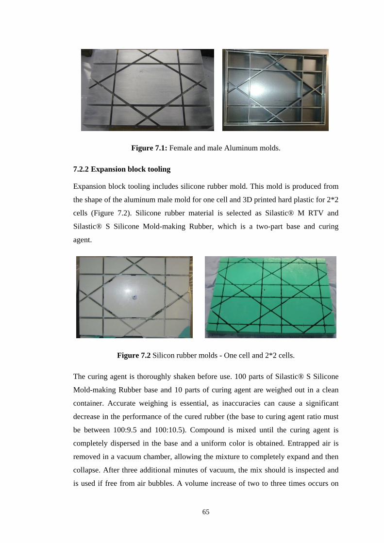
Figure 7.1: Female and male Aluminum molds.
7.2.2 Expansion block tooling
Expansion block tooling includes silicone rubber mold. This mold is produced from
the shape of the aluminum male mold for one cell and 3D printed hard plastic for 2*2
cells (Figure 7.2). Silicone rubber material is selected as Silastic® M RTV and
Silastic® S Silicone Mold-making Rubber, which is a two-part base and curing
agent.
Figure 7.2 Silicon rubber molds - One cell and 2*2 cells.
The curing agent is thoroughly shaken before use. 100 parts of Silastic® S Silicone
Mold-making Rubber base and 10 parts of curing agent are weighed out in a clean
container. Accurate weighing is essential, as inaccuracies can cause a significant
decrease in the performance of the cured rubber (the base to curing agent ratio must
be between 100:9.5 and 100:10.5). Compound is mixed until the curing agent is
completely dispersed in the base and a uniform color is obtained. Entrapped air is
removed in a vacuum chamber, allowing the mixture to completely expand and then
collapse. After three additional minutes of vacuum, the mix should is inspected and
is used if free from air bubbles. A volume increase of two to three times occurs on
65
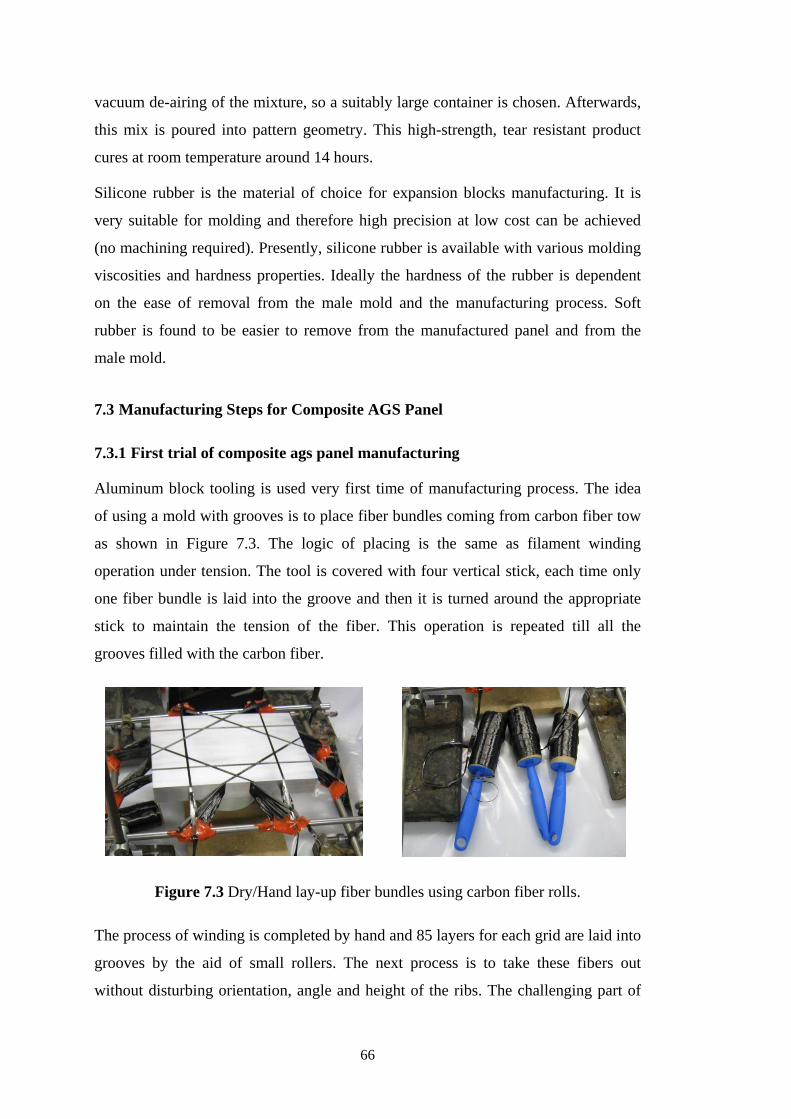
vacuum de-airing of the mixture, so a suitably large container is chosen. Afterwards,
this mix is poured into pattern geometry. This high-strength, tear resistant product
cures at room temperature around 14 hours.
Silicone rubber is the material of choice for expansion blocks manufacturing. It is
very suitable for molding and therefore high precision at low cost can be achieved
(no machining required). Presently, silicone rubber is available with various molding
viscosities and hardness properties. Ideally the hardness of the rubber is dependent
on the ease of removal from the male mold and the manufacturing process. Soft
rubber is found to be easier to remove from the manufactured panel and from the
male mold.
7.3 Manufacturing Steps for Composite AGS Panel
7.3.1 First trial of composite ags panel manufacturing
Aluminum block tooling is used very first time of manufacturing process. The idea
of using a mold with grooves is to place fiber bundles coming from carbon fiber tow
as shown in Figure 7.3. The logic of placing is the same as filament winding
operation under tension. The tool is covered with four vertical stick, each time only
one fiber bundle is laid into the groove and then it is turned around the appropriate
stick to maintain the tension of the fiber. This operation is repeated till all the
grooves filled with the carbon fiber.
Figure 7.3 Dry/Hand lay-up fiber bundles using carbon fiber rolls.
The process of winding is completed by hand and 85 layers for each grid are laid into
grooves by the aid of small rollers. The next process is to take these fibers out
without disturbing orientation, angle and height of the ribs. The challenging part of
66
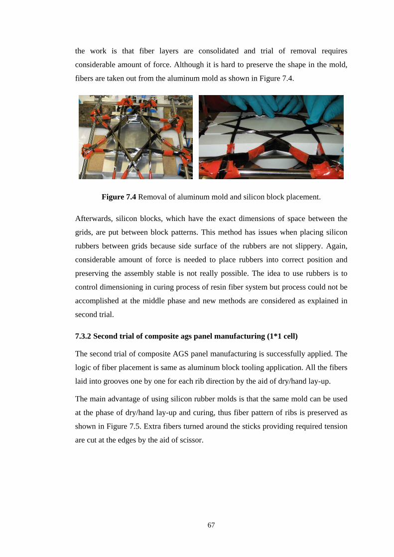
the work is that fiber layers are consolidated and trial of removal requires
considerable amount of force. Although it is hard to preserve the shape in the mold,
fibers are taken out from the aluminum mold as shown in Figure 7.4.
Figure 7.4 Removal of aluminum mold and silicon block placement.
Afterwards, silicon blocks, which have the exact dimensions of space between the
grids, are put between block patterns. This method has issues when placing silicon
rubbers between grids because side surface of the rubbers are not slippery. Again,
considerable amount of force is needed to place rubbers into correct position and
preserving the assembly stable is not really possible. The idea to use rubbers is to
control dimensioning in curing process of resin fiber system but process could not be
accomplished at the middle phase and new methods are considered as explained in
second trial.
7.3.2 Second trial of composite ags panel manufacturing (1*1 cell)
The second trial of composite AGS panel manufacturing is successfully applied. The
logic of fiber placement is same as aluminum block tooling application. All the fibers
laid into grooves one by one for each rib direction by the aid of dry/hand lay-up.
The main advantage of using silicon rubber molds is that the same mold can be used
at the phase of dry/hand lay-up and curing, thus fiber pattern of ribs is preserved as
shown in Figure 7.5. Extra fibers turned around the sticks providing required tension
are cut at the edges by the aid of scissor.
67
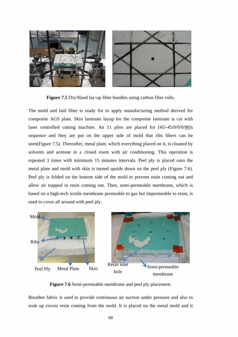
Figure 7.5 Dry/Hand lay-up fiber bundles using carbon fiber rolls.
The mold and laid fiber is ready for to apply manufacturing method derived for
composite AGS plate. Skin laminate layup for the composite laminate is cut with
laser controlled cutting machine. An 11 plies are placed for [45/-45/0/0/0/90]s
sequence and they are put on the upper side of mold that ribs fibers can be
seen(Figure 7.5). Thereafter, metal plate, which everything placed on it, is cleaned by
solvents and acetone in a closed room with air conditioning. This operation is
repeated 3 times with minimum 15 minutes intervals. Peel ply is placed onto the
metal plate and mold with skin is turned upside down on the peel ply (Figure 7.6).
Peel ply is folded on the bottom side of the mold to prevent resin coming out and
allow air trapped in resin coming out. Then, semi-permeable membrane, which is
based on a high-tech textile membrane permeable to gas but impermeable to resin, is
used to cover all around with peel ply.
Figure 7.6 Semi-permeable membrane and peel ply placement.
Breather fabric is used to provide continuous air suction under pressure and also to
soak up excess resin coming from the mold. It is placed on the metal mold and it
Semi-permeable membrane
Peel Ply Skin
Mold
Ribs
Resin inlet hole Metal Plate
68
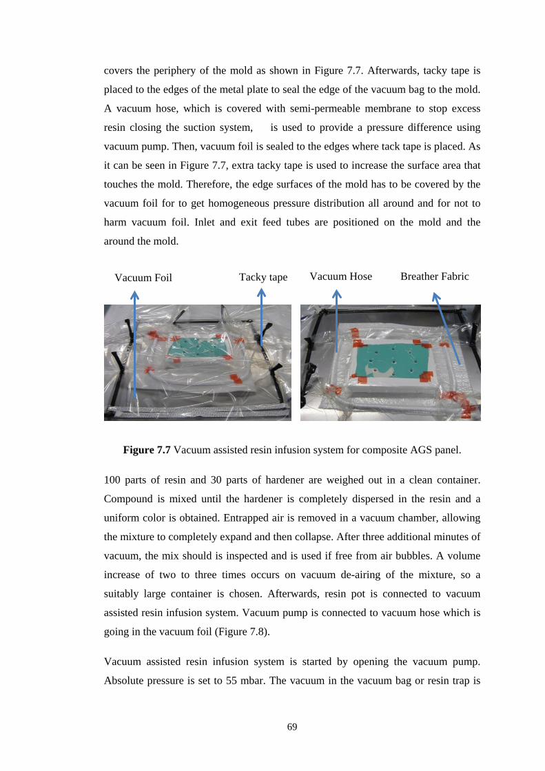
covers the periphery of the mold as shown in Figure 7.7. Afterwards, tacky tape is
placed to the edges of the metal plate to seal the edge of the vacuum bag to the mold.
A vacuum hose, which is covered with semi-permeable membrane to stop excess
resin closing the suction system, is used to provide a pressure difference using
vacuum pump. Then, vacuum foil is sealed to the edges where tack tape is placed. As
it can be seen in Figure 7.7, extra tacky tape is used to increase the surface area that
touches the mold. Therefore, the edge surfaces of the mold has to be covered by the
vacuum foil for to get homogeneous pressure distribution all around and for not to
harm vacuum foil. Inlet and exit feed tubes are positioned on the mold and the
around the mold.
Figure 7.7 Vacuum assisted resin infusion system for composite AGS panel.
100 parts of resin and 30 parts of hardener are weighed out in a clean container.
Compound is mixed until the hardener is completely dispersed in the resin and a
uniform color is obtained. Entrapped air is removed in a vacuum chamber, allowing
the mixture to completely expand and then collapse. After three additional minutes of
vacuum, the mix should is inspected and is used if free from air bubbles. A volume
increase of two to three times occurs on vacuum de-airing of the mixture, so a
suitably large container is chosen. Afterwards, resin pot is connected to vacuum
assisted resin infusion system. Vacuum pump is connected to vacuum hose which is
going in the vacuum foil (Figure 7.8).
Vacuum assisted resin infusion system is started by opening the vacuum pump.
Absolute pressure is set to 55 mbar. The vacuum in the vacuum bag or resin trap is
Vacuum Hose Breather Fabric Vacuum Foil Tacky tape
69
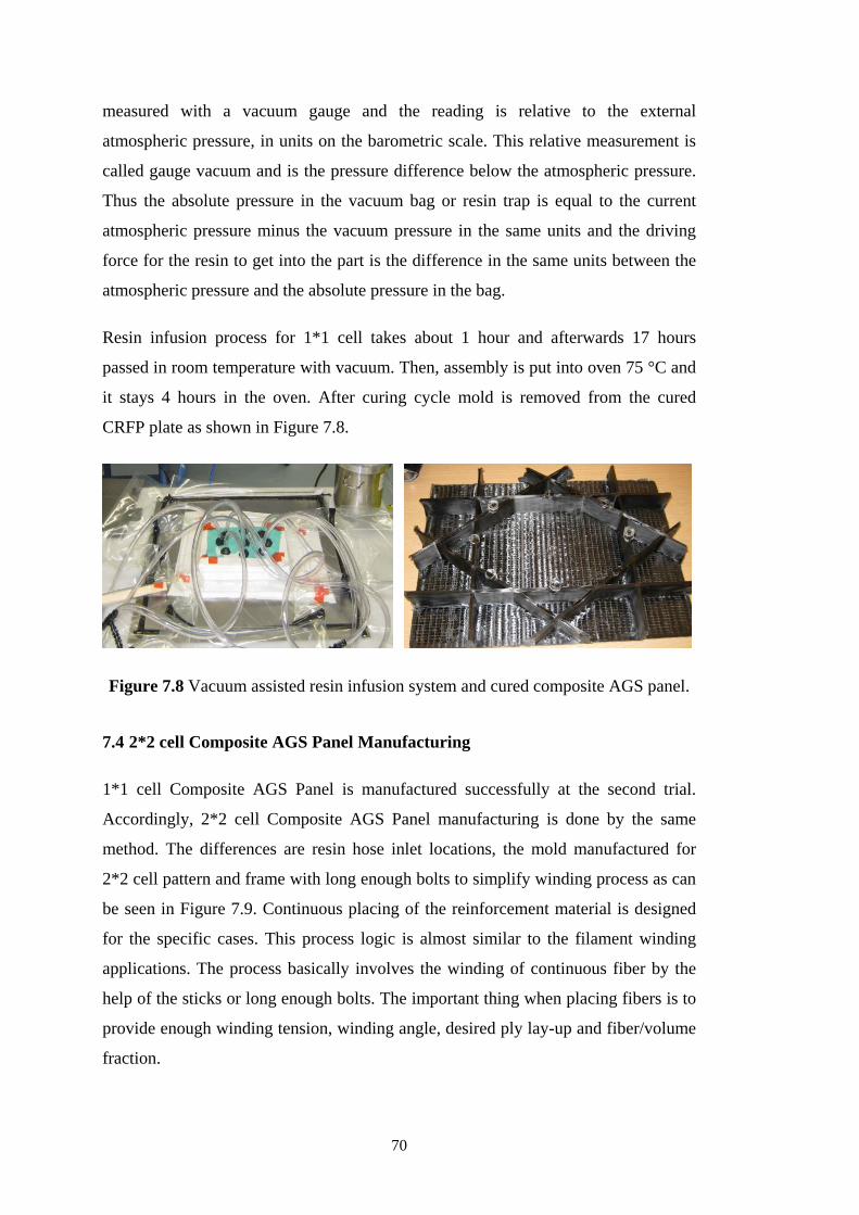
measured with a vacuum gauge and the reading is relative to the external
atmospheric pressure, in units on the barometric scale. This relative measurement is
called gauge vacuum and is the pressure difference below the atmospheric pressure.
Thus the absolute pressure in the vacuum bag or resin trap is equal to the current
atmospheric pressure minus the vacuum pressure in the same units and the driving
force for the resin to get into the part is the difference in the same units between the
atmospheric pressure and the absolute pressure in the bag.
Resin infusion process for 1*1 cell takes about 1 hour and afterwards 17 hours
passed in room temperature with vacuum. Then, assembly is put into oven 75 °C and
it stays 4 hours in the oven. After curing cycle mold is removed from the cured
CRFP plate as shown in Figure 7.8.
Figure 7.8 Vacuum assisted resin infusion system and cured composite AGS panel.
7.4 2*2 cell Composite AGS Panel Manufacturing
1*1 cell Composite AGS Panel is manufactured successfully at the second trial.
Accordingly, 2*2 cell Composite AGS Panel manufacturing is done by the same
method. The differences are resin hose inlet locations, the mold manufactured for
2*2 cell pattern and frame with long enough bolts to simplify winding process as can
be seen in Figure 7.9. Continuous placing of the reinforcement material is designed
for the specific cases. This process logic is almost similar to the filament winding
applications. The process basically involves the winding of continuous fiber by the
help of the sticks or long enough bolts. The important thing when placing fibers is to
provide enough winding tension, winding angle, desired ply lay-up and fiber/volume
fraction.
70
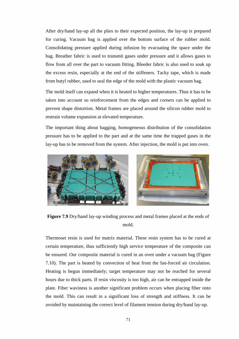
After dry/hand lay-up all the plies to their expected position, the lay-up is prepared
for curing. Vacuum bag is applied over the bottom surface of the rubber mold.
Consolidating pressure applied during infusion by evacuating the space under the
bag. Breather fabric is used to transmit gases under pressure and it allows gases to
flow from all over the part to vacuum fitting. Bleeder fabric is also used to soak up
the excess resin, especially at the end of the stiffeners. Tacky tape, which is made
from butyl rubber, used to seal the edge of the mold with the plastic vacuum bag.
The mold itself can expand when it is heated to higher temperatures. Thus it has to be
taken into account so reinforcement from the edges and corners can be applied to
prevent shape distortion. Metal frames are placed around the silicon rubber mold to
restrain volume expansion at elevated temperature.
The important thing about bagging, homogeneous distribution of the consolidation
pressure has to be applied to the part and at the same time the trapped gases in the
lay-up has to be removed from the system. After injection, the mold is put into oven.
Figure 7.9 Dry/hand lay-up winding process and metal frames placed at the ends of
mold.
Thermoset resin is used for matrix material. These resin system has to be cured at
certain temperature, thus sufficiently high service temperature of the composite can
be ensured. Our composite material is cured in an oven under a vacuum bag (Figure
7.10). The part is heated by convection of heat from the fan-forced air circulation.
Heating is begun immediately; target temperature may not be reached for several
hours due to thick parts. If resin viscosity is too high, air can be entrapped inside the
plate. Fiber waviness is another significant problem occurs when placing fiber onto
the mold. This can result in a significant loss of strength and stiffness. It can be
avoided by maintaining the correct level of filament tension during dry/hand lay-up.
71
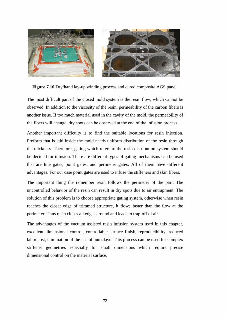
Figure 7.10 Dry/hand lay-up winding process and cured composite AGS panel.
The most difficult part of the closed mold system is the resin flow, which cannot be
observed. In addition to the viscosity of the resin, permeability of the carbon fibers is
another issue. If too much material used in the cavity of the mold, the permeability of
the fibers will change, dry spots can be observed at the end of the infusion process.
Another important difficulty is to find the suitable locations for resin injection.
Preform that is laid inside the mold needs uniform distribution of the resin through
the thickness. Therefore, gating which refers to the resin distribution system should
be decided for infusion. There are different types of gating mechanisms can be used
that are line gates, point gates, and perimeter gates. All of them have different
advantages. For our case point gates are used to infuse the stiffeners and skin fibers.
The important thing the remember resin follows the perimeter of the part. The
uncontrolled behavior of the resin can result in dry spots due to air entrapment. The
solution of this problem is to choose appropriate gating system, otherwise when resin
reaches the closer edge of trimmed structure, it flows faster than the flow at the
perimeter. Thus resin closes all edges around and leads to trap-off of air.
The advantages of the vacuum assisted resin infusion system used in this chapter,
excellent dimensional control, controllable surface finish, reproducibility, reduced
labor cost, elimination of the use of autoclave. This process can be used for complex
stiffener geometries especially for small dimensions which require precise
dimensional control on the material surface.
72
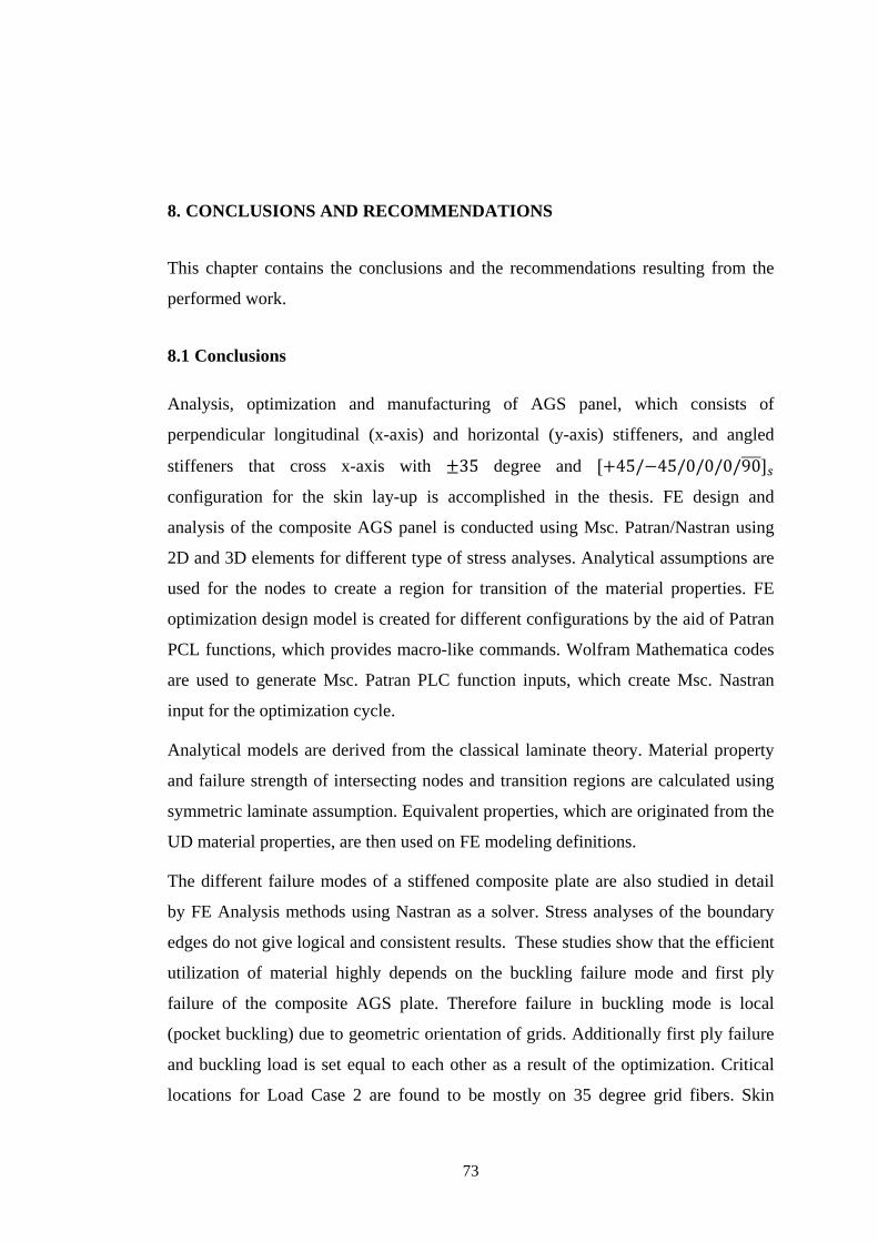
8. CONCLUSIONS AND RECOMMENDATIONS
This chapter contains the conclusions and the recommendations resulting from the
performed work.
8.1 Conclusions
Analysis, optimization and manufacturing of AGS panel, which consists of
perpendicular longitudinal (x-axis) and horizontal (y-axis) stiffeners, and angled
stiffeners that cross x-axis with ±35 degree and [+45/−45/0/0/0/90����]𝑠
configuration for the skin lay-up is accomplished in the thesis. FE design and
analysis of the composite AGS panel is conducted using Msc. Patran/Nastran using
2D and 3D elements for different type of stress analyses. Analytical assumptions are
used for the nodes to create a region for transition of the material properties. FE
optimization design model is created for different configurations by the aid of Patran
PCL functions, which provides macro-like commands. Wolfram Mathematica codes
are used to generate Msc. Patran PLC function inputs, which create Msc. Nastran
input for the optimization cycle.
Analytical models are derived from the classical laminate theory. Material property
and failure strength of intersecting nodes and transition regions are calculated using
symmetric laminate assumption. Equivalent properties, which are originated from the
UD material properties, are then used on FE modeling definitions.
The different failure modes of a stiffened composite plate are also studied in detail
by FE Analysis methods using Nastran as a solver. Stress analyses of the boundary
edges do not give logical and consistent results. These studies show that the efficient
utilization of material highly depends on the buckling failure mode and first ply
failure of the composite AGS plate. Therefore failure in buckling mode is local
(pocket buckling) due to geometric orientation of grids. Additionally first ply failure
and buckling load is set equal to each other as a result of the optimization. Critical
locations for Load Case 2 are found to be mostly on 35 degree grid fibers. Skin
73
material thickness has significant effect on the buckling modes of the composite
AGS panel.
Manufacturing of the AGS panel use methods of resin infusion process under
vacuum and quality evaluation of the AGS panel is conducted macroscopic methods
to check. Designed methodology for manufacturing gives reliable material with low
cost production technique. Resin infusion for advanced composite structures is
highly desired due to its low cost and less time spent for manufacturing, although
uncontrollable variables exist in infusion process. Therefore selected method
provides an excellent method when it is compared to studies done so far. Fiber
volume is reached up to 55% and dimensioning of the manufactured part complies
with the design model. Material quality evaluation is done by macro pictures of the
manufactured material by human eye. The quality for the grids is beyond the
expectations, although small dimensions of the grids make things difficult.
8.2 Recommendations
Analysis, optimization and manufacturing of AGS panel needs development as all
the studies on the literature. There are number of revisions and validations on all the
steps of the composite AGS plate project.
First of all, 2D FE analysis elements can be extended to thick composite elements or
3D analysis of the whole composite plate to validate the results coming from this
thesis with the more detailed analysis.
Secondly, optimization cycles used in Nastran codes can be extended to genetic
algorithms, thus a better converged optimum can be obtained from optimization
cycle. Design constraints might give other optimums; therefore a new design model
can be analyzed in detail.
Thirdly, theoretical model creation cycle might be validated by the relevant tests or
historical test data if possible for the material properties derived.
Furthermore, manufacturing of the AGS composite plate needs input for resin inlet
and its location changes for the different numbers of cells. Accordingly, an algorithm
might be developed to locate resin inlets for different type of dimensioning and
geometries.
74

In this way, quality control tests to get fiber volume fraction is needed. Deficiencies
that are possible due to manufacturing methods have to be inspected in material
testing and inspection laboratory.
It could also be said that, manufacturing of the composite AGS panel with dry/hand
lay-up is time consuming. Thus, a filament winding method might be designed to
automate winding phase which will allow manufacturing fuselage structure.
Subsequently, material testing and microscopy might be designed for to validate the
analysis results and material quality.
75

76
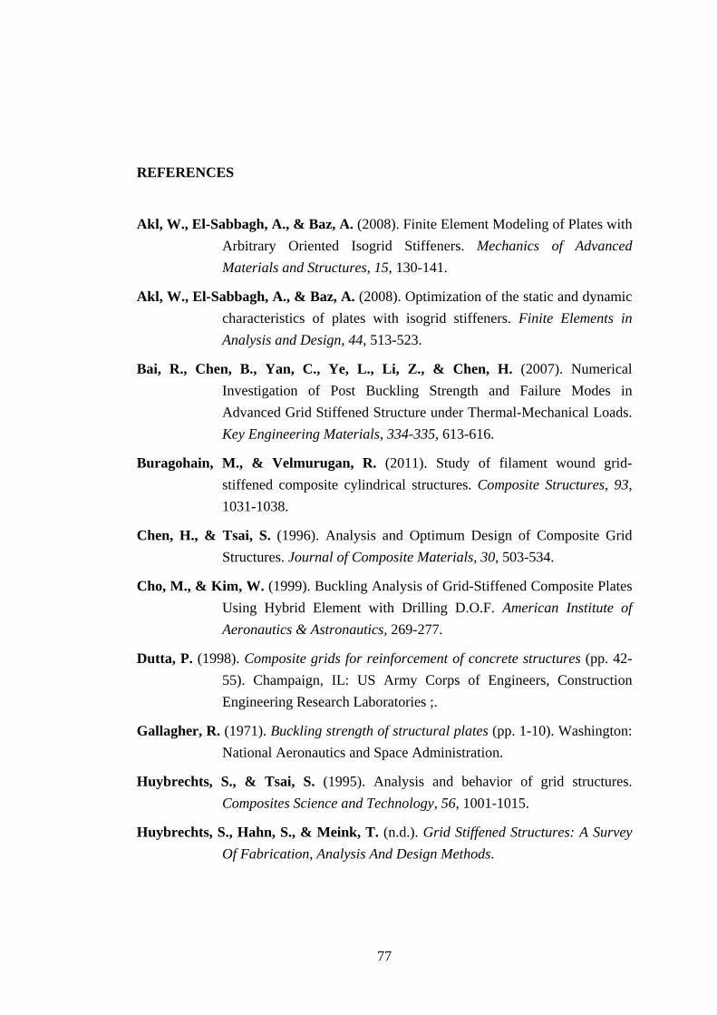
REFERENCES
Akl, W., El-Sabbagh, A., & Baz, A. (2008). Finite Element Modeling of Plates with Arbitrary Oriented Isogrid Stiffeners. Mechanics of Advanced Materials and Structures, 15, 130-141.
Akl, W., El-Sabbagh, A., & Baz, A. (2008). Optimization of the static and dynamic characteristics of plates with isogrid stiffeners. Finite Elements in Analysis and Design, 44, 513-523.
Bai, R., Chen, B., Yan, C., Ye, L., Li, Z., & Chen, H. (2007). Numerical Investigation of Post Buckling Strength and Failure Modes in Advanced Grid Stiffened Structure under Thermal-Mechanical Loads. Key Engineering Materials, 334-335, 613-616.
Buragohain, M., & Velmurugan, R. (2011). Study of filament wound grid-stiffened composite cylindrical structures. Composite Structures, 93, 1031-1038.
Chen, H., & Tsai, S. (1996). Analysis and Optimum Design of Composite Grid Structures. Journal of Composite Materials, 30, 503-534.
Cho, M., & Kim, W. (1999). Buckling Analysis of Grid-Stiffened Composite Plates Using Hybrid Element with Drilling D.O.F. American Institute of Aeronautics & Astronautics, 269-277.
Dutta, P. (1998). Composite grids for reinforcement of concrete structures (pp. 42-55). Champaign, IL: US Army Corps of Engineers, Construction Engineering Research Laboratories ;.
Gallagher, R. (1971). Buckling strength of structural plates (pp. 1-10). Washington: National Aeronautics and Space Administration.
Huybrechts, S., & Tsai, S. (1995). Analysis and behavior of grid structures. Composites Science and Technology, 56, 1001-1015.
Huybrechts, S., Hahn, S., & Meink, T. (n.d.). Grid Stiffened Structures: A Survey Of Fabrication, Analysis And Design Methods.
77
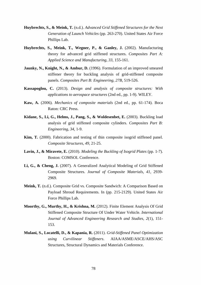
Huybrechts, S., & Meink, T. (n.d.). Advanced Grid Stiffened Structures for the Next Generation of Launch Vehicles (pp. 263-270). United States Air Force Phillips Lab.
Huybrechts, S., Meink, T., Wegner, P., & Ganley, J. (2002). Manufacturing theory for advanced grid stiffened structures. Composites Part A: Applied Science and Manufacturing, 33, 155-161.
Jaunky, N., Knight, N., & Ambur, D. (1996). Formulation of an improved smeared stiffener theory for buckling analysis of grid-stiffened composite panels. Composites Part B: Engineering, 27B, 519-526.
Kassapoglou, C. (2013). Design and analysis of composite structures: With applications to aerospace structures (2nd ed., pp. 1-9). WILEY.
Kaw, A. (2006). Mechanics of composite materials (2nd ed., pp. 61-174). Boca Raton: CRC Press.
Kidane, S., Li, G., Helms, J., Pang, S., & Woldesenbet, E. (2003). Buckling load analysis of grid stiffened composite cylinders. Composites Part B: Engineering, 34, 1-9.
Kim, T. (2000). Fabrication and testing of thin composite isogrid stiffened panel. Composite Structures, 49, 21-25.
Lavin, J., & Miravete, E. (2010). Modeling the Buckling of Isogrid Plates (pp. 1-7). Boston: COMSOL Conference.
Li, G., & Cheng, J. (2007). A Generalized Analytical Modeling of Grid Stiffened Composite Structures. Journal of Composite Materials, 41, 2939-2969.
Meink, T. (n.d.). Composite Grid vs. Composite Sandwich: A Comparison Based on Payload Shroud Requirements. In (pp. 215-2129). United States Air Force Phillips Lab.
Moorthy, G., Murthy, H., & Krishna, M. (2012). Finite Element Analysis Of Grid Stiffened Composite Structure Of Under Water Vehicle. International Journal of Advanced Engineering Research and Studies, 2(1), 151-153.
Mulani, S., Locatelli, D., & Kapania, R. (2011). Grid-Stiffened Panel Optimization using Curvilinear Stiffeners. AIAA/ASME/ASCE/AHS/ASC Structures, Structural Dynamics and Materials Conference.
78
Niu, M. (1992). Composite Airframe Structures (1st ed., p. 1). Los Angeles, Calif.: University of California.
Phillips, J., & Gürdal, Z. (1990). Structural analysis and optimum design of geodesically stiffened composite panels (pp. 15,45-50). Blacksburg, Va.: Virginia Polytechnic Institute and State University, Center for Composite Materials and Structures.
Prusty, B., & Satsangi, S. (2001). Finite element buckling analysis of laminated composite stiffened shells. International Journal of Crashworthiness, 471-484.
Ray, C., & Satsangi, S. (1999). Laminated Stiffened Plate-A First Ply Failure Analysis. Journal of Reinforced Plastics and Composites, 18, 1061-1076.
Rehfield, L., & Deo, R. (1978). Buckling of Continuous Filament Advanced Composite Isogrid Wide Columns in Axial Compression (pp. 1-5). Ft. Belvoir: Defense Technical Information Center.
Slysh, P. (n.d.). Isogrid Structure Technology and Applications (pp. 1-5). California: General Dynamics Convair Division.
Tsai, S. (n.d.). Structural Behaviour of Composite Materials. California: PHILCO CORPORATION.
Wegner, P., Higgins, J., & VanWest, B. (2002). Application of Advanced Grid-Stiffened Structures Technology to the Minotaur Payload Fairing (pp. 1-7). Ft. Belvoir: Defense Technical Information Center.
Wodesenbet, E., Kidane, S., & Pang, S. (2003). Optimization for buckling loads of grid stiffened composite panels. Composite Structures, 60, 159-169.
79

80

APPENDICES
APPENDIX A: Maximum Ply Stresses on Ribs for LC1 and LC3
APPENDIX B: MSC. Patran Composite Material Definitions
81
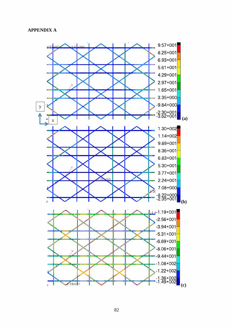
APPENDIX A
(a)
(b)
(c)
x
y
82
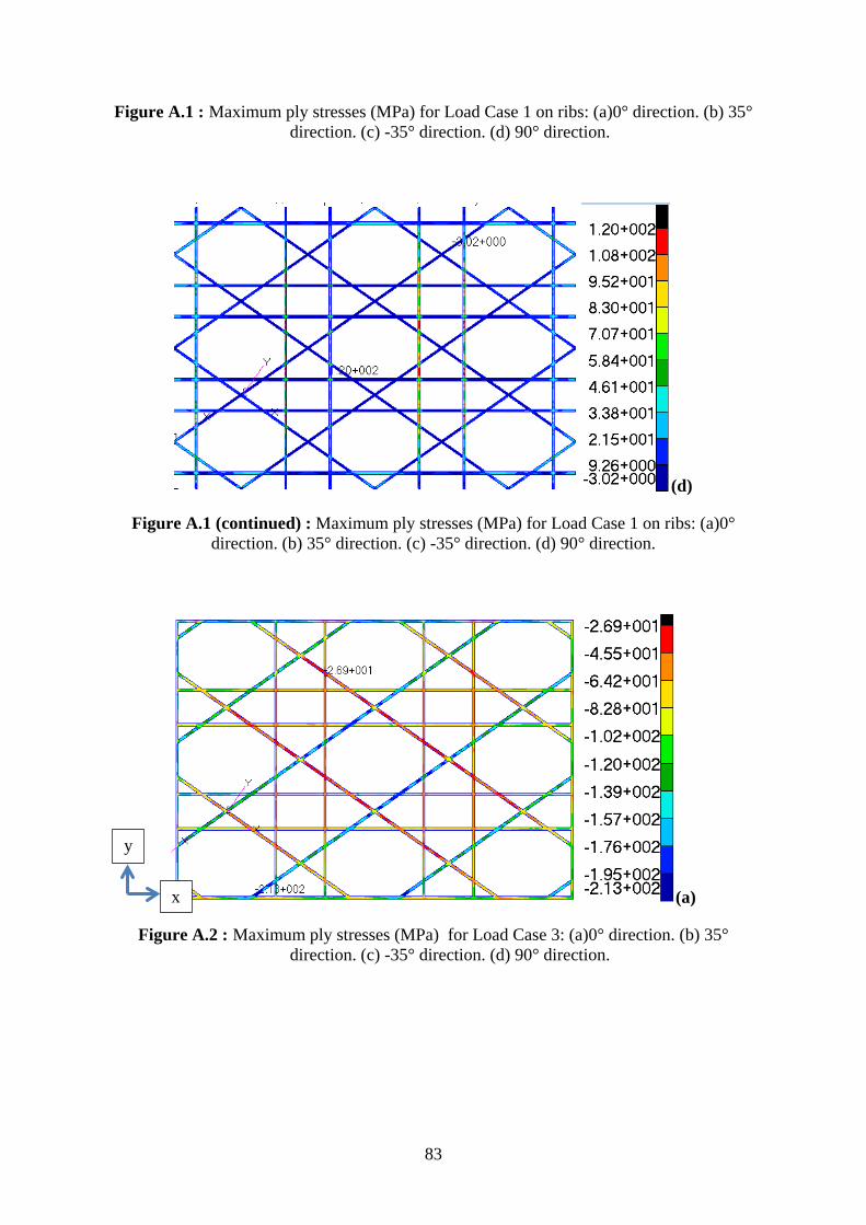
Figure A.1 : Maximum ply stresses (MPa) for Load Case 1 on ribs: (a)0° direction. (b) 35° direction. (c) -35° direction. (d) 90° direction.
(d)
Figure A.1 (continued) : Maximum ply stresses (MPa) for Load Case 1 on ribs: (a)0° direction. (b) 35° direction. (c) -35° direction. (d) 90° direction.
(a)
Figure A.2 : Maximum ply stresses (MPa) for Load Case 3: (a)0° direction. (b) 35° direction. (c) -35° direction. (d) 90° direction.
x
y
83
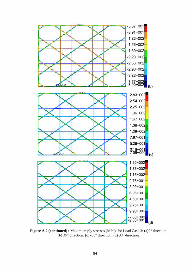
(b)
(c)
(d)
Figure A.2 (continued) : Maximum ply stresses (MPa) for Load Case 3: (a)0° direction. (b) 35° direction. (c) -35° direction. (d) 90° direction.
84
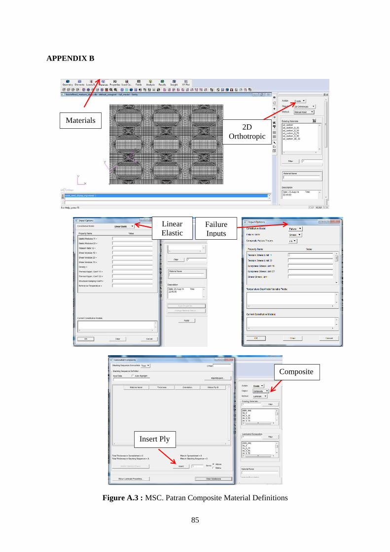
APPENDIX B
Figure A.3 : MSC. Patran Composite Material Definitions
Materials 2D
Orthotropic
Composite
Failure Inputs
Linear Elastic
Insert Ply
85

86
CURRICULUM VITAE
Name Surname: Onur COŞKUN
Place and Date of Birth: İskenderun / 30.06.1987
Address: Kurtköy / İstanbul
E-Mail: [email protected]
B.Sc.: Istanbul Technical University
Professional Experience and Rewards:
-
List of Publications and Patents:
-
PUBLICATIONS/PRESENTATIONS ON THE THESIS
-
87