core.ac.uk · Published by Oxford University Press on behalf of The Royal ... counter-clockwise rotation of ... crust and perhaps the upper few tens of kilometres

This is a repository copy of Crustal structure of the carpathian-pannonian region from ambient noise tomography.

White Rose Research Online URL for this paper:http://eprints.whiterose.ac.uk/80165/

Version: Published Version

Article:

Ren, Y, Stuart, G, Houseman, G et al. (26 more authors) (2013) Crustal structure of the carpathian-pannonian region from ambient noise tomography. Geophysical Journal International, 195 (2). 1351 - 1369. ISSN 0956-540X

https://doi.org/10.1093/gji/ggt316

[email protected]://eprints.whiterose.ac.uk/

Reuse

Unless indicated otherwise, fulltext items are protected by copyright with all rights reserved. The copyright exception in section 29 of the Copyright, Designs and Patents Act 1988 allows the making of a single copy solely for the purpose of non-commercial research or private study within the limits of fair dealing. The publisher or other rights-holder may allow further reproduction and re-use of this version - refer to the White Rose Research Online record for this item. Where records identify the publisher as the copyright holder, users can verify any specific terms of use on the publisher’s website.

Takedown

If you consider content in White Rose Research Online to be in breach of UK law, please notify us by emailing [email protected] including the URL of the record and the reason for the withdrawal request.

mailto:[email protected]

https://eprints.whiterose.ac.uk/

Geophysical Journal InternationalGeophys. J. Int.(2013)195, 1351–1369 doi: 10.1093/gji/ggt316Advance Access publication 2013 September 6

GJI

Sei

smolo

gy

Crustal structure of the Carpathian–Pannonian region from ambientnoise tomography

Yong Ren,1 Bogdan Grecu,2 Graham Stuart,1 Gregory Houseman,1 Endre Hegedus3

and South Carpathian Project Working Group1School of Earth and Environment, University of Leeds, Leeds, LS2 9JT, UK. E-mail: [email protected] Institute of Earth Physics, P.O. Box MG-21, Bucharest-Magurele, Romania3Eotvos Lorand Geophysical Institute,1145Budapest, Kolumbusz u.17-23, Hungary

Accepted 2013 August 5. Received 2013 June 3; in original form 2013 January 18

S U M M A R Y

We use ambient noise tomography to investigate the crust and uppermost mantle structurebeneath the Carpathian–Pannonian region of Central Europe. Over 7500 Rayleigh wave em-pirical Green’s functions are derived from interstation cross-correlations of vertical componentambient seismic noise recordings (2005–2011) using a temporary network of 54 stations de-ployed during the South Carpathian Project (2009–2011), 56 temporary stations deployedin the Carpathian Basins Project (2005–2007) and 100 permanent and regional broad-bandstations. Rayleigh wave group velocity dispersion curves (4–40 s) are determined using themultiple-filter analysis technique. Group velocity maps are computed on a grid of 0.2◦ × 0.2◦

from a non-linear 2-D tomographic inversion using the subspace method. We then invertedthe group velocity maps for the 3-D shear wave velocity structure of the crust and uppermostmantle beneath the region. Our shear wave velocity model provides a uniquely complete andrelatively high-resolution view of the crustal structure in the Carpathian–Pannonian region,which in general is validated by comparison with previous studies using other methods toprobe the crustal structure. At shallow depths (<10 km) we find relatively high velocitiesbelow where basement is exposed (e.g. Bohemian Massif, Eastern Alps, most of Carpathians,Apuseni Mountains and Trans-Danubian Ranges) whereas sedimentary areas (e.g. Vienna,Pannonian, Transylvanian and Focsani Basins) are associated with low velocities of well de-fined depth extent. The mid to lower crust (16–34 km) below the Mid-Hungarian Line isassociated with a broad NE–SW trending relatively fast anomaly, flanked to the NW by anelongated low-velocity region beneath the Trans-Danubian Ranges. In the lowermost crust anduppermost mantle (between 30 and 40 km), relatively low velocities are observed beneath theBohemian Massif and Eastern Alps but the most striking features are the broad low velocityregions beneath the Apuseni Mountains and most of the Carpathian chain, which likely isexplained by relatively thick crust. Finally, most of the Pannonian and Vienna Basin regions atdepths>30 km are relatively fast, presumably related to shallowing of the Moho consequenton the extensional history of the Pannonian region.

Key words: Surface waves and free oscillations; Seismic tomography; Crustal structure;Europe.

1 I N T RO D U C T I O N

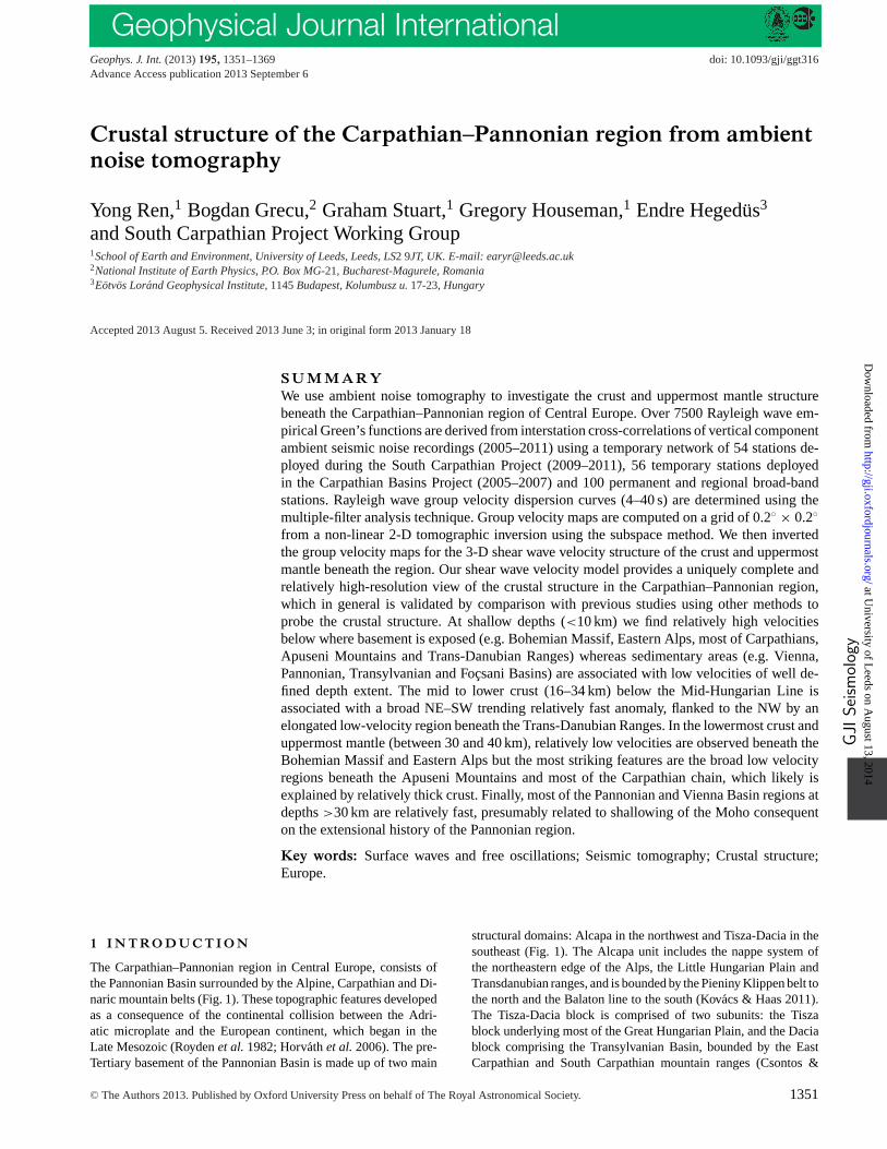
The Carpathian–Pannonian region in Central Europe, consists ofthe Pannonian Basin surrounded by the Alpine, Carpathian and Di-naric mountain belts (Fig. 1). These topographic features developedas a consequence of the continental collision between the Adri-atic microplate and the European continent, which began in theLate Mesozoic (Roydenet al.1982; Horvathet al.2006). The pre-Tertiary basement of the Pannonian Basin is made up of two main

structural domains: Alcapa in the northwest and Tisza-Dacia in thesoutheast (Fig. 1). The Alcapa unit includes the nappe system ofthe northeastern edge of the Alps, the Little Hungarian Plain andTransdanubian ranges, and is bounded by the Pieniny Klippen belt tothe north and the Balaton line to the south (Kovacs & Haas 2011).The Tisza-Dacia block is comprised of two subunits: the Tiszablock underlying most of the Great Hungarian Plain, and the Daciablock comprising the Transylvanian Basin, bounded by the EastCarpathian and South Carpathian mountain ranges (Csontos &

C© The Authors 2013. Published by Oxford University Press on behalf of The Royal Astronomical Society. 1351

at University of Leeds on A

ugust 13, 2014http://gji.oxfordjournals.org/

Dow

nloaded from

http://gji.oxfordjournals.org/

1352 Y. Renet al.

Figure 1. Topographic map of the Carpathian–Pannonian system with surface structural features: red filled patterns indicate outcrops of calc-alkaline andsilicic volcanic rocks after Harangi & Lenkey (2007); black lines show some of the major faults. CSVF, Central Slovakian volcanic field; PAL, Peri-AdriaticLine; MHL, Mid-Hungarian Line; BL, Balaton Line; PKB, Pieniny Klippen Belt; VZ, Vrancea Zone.

Voros 2004). During the Neogene, the Alcapa unit underwent a netcounter-clockwise rotation of about 50◦–70◦ and was translated tothe ENE (Marton & Fodor 1995), whereas the Tisza-Dacia unit ro-tated clockwise 90◦ (Patrascuet al.1994). The rotation of these twoblocks was accompanied by extension during the Miocene, whichled to the formation of the Pannonian Basin. Several theories pro-posed to explain the formation of this basin include extension dueto the eastward rollback of a subducted slab (Horvathet al. 1993,2006) and/or gravitational collapse of former overthickened oro-genic terrain (Gemmer & Houseman 2007). The Pannonian Basinincludes a set of small, deep subbasins (some can exceed 7 kmin thickness), separated by relatively shallow basement blocks andfilled with Neogene-Quaternary sediments (Tariet al.1999).

Constraining crustal and lithospheric structures in theCarpathian–Pannonian region is crucial for a better understand-ing of the dynamic processes that determined the tectonic evolutionof the region. Previous seismological investigations of the crustalstructure in the region are mainly based on controlled-source seis-mic reflection/refraction studies on 2-D profiles. There is reasonablecontrol on crustal structure in the western part of the Carpathian–Pannonian region from CELEBRATION 2000 (Guterchet al.2003;Gradet al.2008), ALP 2002 (Bruckl et al.2003; Behmet al.2007)and SUDETES 2003 (Gradet al.2003, 2008) seismic experiments.In contrast, the eastern part of the Carpathian–Pannonian region haslimited coverage with the VRANCEA 2001 refraction line (Hauser

et al.2007), the combined DRACULA I and DACIA-PLAN reflec-tion line (Fillerup et al. 2010) crossing the Transylvanian Basin,Vrancea Zone and Focsani Basin. 3-D seismic velocity models forthe Vrancea region incorporating converted phase measurementsfrom local and teleseismic sources have also been developed byMartinet al.(2005) and Ivan (2011). Although those studies provideimportant measurements of crustal structure which have been influ-ential in geodynamic interpretations, other parts of the region (forexample, the Apuseni Mountains of Romania) are almost uncon-strained by seismic measurements of the crust. To date, the availableregional crustal models (e.g. Bassinet al.2000; Tesauroet al.2008;Gradet al.2009) are essentially based on a sparse network of refrac-tion lines interpolated across the unsampled regions. Surface wavetomography, derived from ambient seismic noise analysis, repre-sents an alternative seismic technique that provides important new,relatively high-resolution, constraints on the 3-D crustal structureof the region.

Ambient noise tomography has proven particularly powerful inimaging the Earth’s crust and uppermost mantle in the last decade,at both regional and global scale beneath dense seismic arrays (e.g.Shapiroet al.2005; Yaoet al.2006; Linet al.2007; Moschettiet al.2007; Yanget al.2007; Liet al.2009; Arroucauet al.2010; Saygin& Kennett 2012). The technique is based on the principle that anestimate of surface wave Green’s functions between two stationscan be retrieved from cross-correlation of ambient seismic noise



Dow

nloaded from


Crust of the Carpathian–Pannonian region 1353

records (Weaver & Lobkis 2001; Derodeet al.2003; Snieder 2004;Wapenaar 2004; Laroseet al.2005). Ambient noise tomography hasthe advantage of not depending on the distribution of earthquakesources as in classical interstation surface wave tomography; evenif the noise is anisotropic, resolution is essentially limited by thedistribution of stations and the frequencies present in the seismicwavefield. The short to intermediate-period dispersion curve mea-surements that constrain the crust and uppermost mantle structures,can be more effectively retrieved from ambient noise analysis thanfrom the surface wave signals of seismic events. Here, we presentRayleigh-wave group velocity maps for period range 4–40 s, and in-terpret crustal and uppermost mantle shear wave velocity structuresfrom ambient noise tomography, using data from a uniquely densenetwork of permanent and temporary broad-band seismic stationsin the Carpathian–Pannonian region.

2 DATA P RO C E S S I N G

A N D M E A S U R E M E N T

2.1 Data

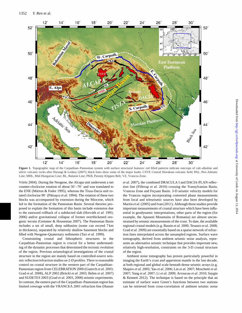
We assembled continuous broad-band vertical component seismicdata recorded on 207 stations in the Carpathian–Pannonian region

(Fig. 2) from four sources: South Carpathian Project (SCP, 2009–2011, Renet al. 2012), Carpathian Basins Project (CBP, 2005–2007; Dandoet al. 2011), Romanian National Seismic Network(http://www.infp.ro) and other permanent stations available frominternational data centres. The South Carpathian Project was amajor collaborative seismological project between the Universityof Leeds, Eotvos Lorand Geophysical Institute (ELGI), Budapest,Hungary; National Institute of Earth Physics (NIEP), Bucharest,Romania and the State Seismological Survey of Serbia (RSZ), Bel-grade, Serbia. The SCP temporary network (Fig. 2) consisted of17 CMG-40T, 13 CMG-3T and 24 CMG-6TD sensors, installedacross the eastern Pannonian Basin, Transylvanian Basin and theSouth Carpathian Mountains in Hungary, Romania and Serbia, be-tween June 2009 and June 2011 (Renet al.2012). The CarpathianBasins Project was a collaborative seismic experiment deployed byUniversity of Leeds, ELGI, RSZ and TU-Wien (Technische Univer-sitat Wien, Austria) between October 2005 and August 2007. TheCBP temporary network (Fig. 2) consisted of 46 CMG-6TD and10 CMG-3T(D) sensors, installed across Eastern Austria, WesternHungary, Northern Serbia and Croatia (Dandoet al. 2011). Threeof these broad-band stations were in operation during the wholeperiod covering both the CBP and SCP experiments. We have alsoused data from 30 broad-band temporary and permanent stations of

Figure 2. Distribution of broad-band stations used in this study. Blue squares represent stations of the temporary network deployed in the South CarpathianProject (SCP, 2009–2011; Renet al. 2012). Brown hexagons mark stations from the temporary network deployed in the Carpathian Basins Project (CBP,2005–2007; Dandoet al. 2011). Red diamonds represent stations which were in operation in both CBP and SCP experiments. White inverted trianglesdepict additional permanent broad-band stations used in this study. Yellow triangles represent seismic stations from the Romanian Regional Seismic Network(http://www.infp.ro).



Dow

nloaded from


1354 Y. Renet al.

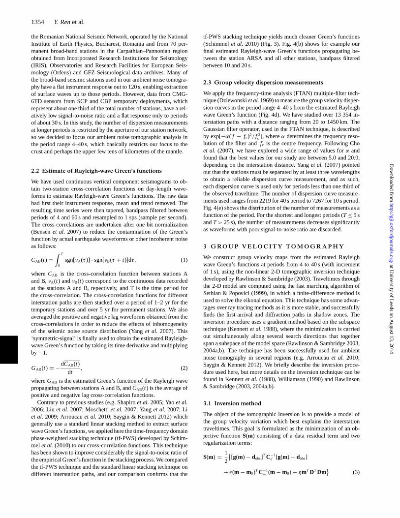
the Romanian National Seismic Network, operated by the NationalInstitute of Earth Physics, Bucharest, Romania and from 70 per-manent broad-band stations in the Carpathian–Pannonian regionobtained from Incorporated Research Institutions for Seismology(IRIS), Observatories and Research Facilities for European Seis-mology (Orfeus) and GFZ Seismological data archives. Many ofthe broad-band seismic stations used in our ambient noise tomogra-phy have a flat instrument response out to 120 s, enabling extractionof surface waves up to those periods. However, data from CMG-6TD sensors from SCP and CBP temporary deployments, whichrepresent about one third of the total number of stations, have a rel-atively low signal-to-noise ratio and a flat response only to periodsof about 30 s. In this study, the number of dispersion measurementsat longer periods is restricted by the aperture of our station network,so we decided to focus our ambient noise tomographic analysis inthe period range 4–40 s, which basically restricts our focus to thecrust and perhaps the upper few tens of kilometres of the mantle.

2.2 Estimate of Rayleigh-wave Green’s functions

We have used continuous vertical component seismograms to ob-tain two-station cross-correlation functions on day-length wave-forms to estimate Rayleigh-wave Green’s functions. The raw datahad first their instrument response, mean and trend removed. Theresulting time series were then tapered, bandpass filtered betweenperiods of 4 and 60 s and resampled to 1 sps (sample per second).The cross-correlations are undertaken after one-bit normalization(Bensenet al. 2007) to reduce the contamination of the Green’sfunction by actual earthquake waveforms or other incoherent noiseas follows:

CAB(t) =∫ T

0sgn[νA(τ )] · sgn[νB(τ + t)]dτ, (1)

where CAB is the cross-correlation function between stations Aand B,νA(t) andνB(t) correspond to the continuous data recordedat the stations A and B, repectively, and T is the time period forthe cross-correlation. The cross-correlation functions for differentinterstation paths are then stacked over a period of 1–2 yr for thetemporary stations and over 5 yr for permanent stations. We alsoaveraged the positive and negative lag waveforms obtained from thecross-correlations in order to reduce the effects of inhomogeneityof the seismic noise source distribution (Yanget al. 2007). This‘symmetric-signal’ is finally used to obtain the estimated Rayleigh-wave Green’s function by taking its time derivative and multiplyingby −1.

GAB(t) = −dCAB(t)

dt, (2)

whereGAB is the estimated Green’s function of the Rayleigh wavepropagating between stations A and B, andCAB(t) is the average ofpositive and negative lag cross-correlation functions.

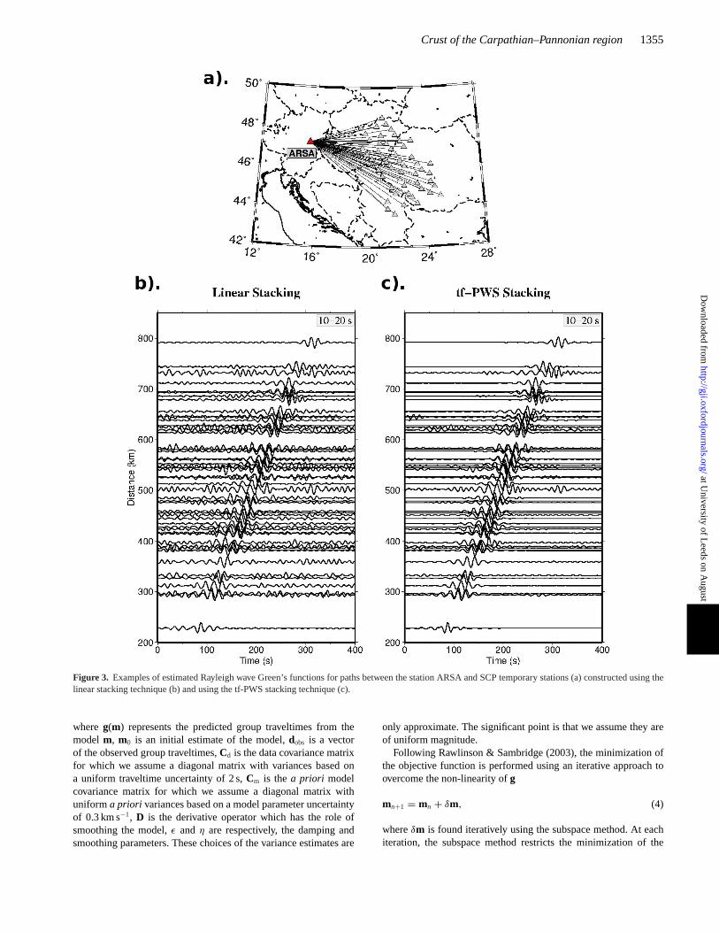
Contrary to previous studies (e.g. Shapiroet al.2005; Yaoet al.2006; Linet al. 2007; Moschettiet al. 2007; Yanget al. 2007; Liet al. 2009; Arroucauet al. 2010; Saygin & Kennett 2012) whichgenerally use a standard linear stacking method to extract surfacewave Green’s functions, we applied here the time-frequency domainphase-weighted stacking technique (tf-PWS) developed by Schim-melet al. (2010) to our cross-correlation functions. This techniquehas been shown to improve considerably the signal-to-noise ratio ofthe empirical Green’s function in the stacking process. We comparedthe tf-PWS technique and the standard linear stacking technique ondifferent interstation paths, and our comparison confirms that the

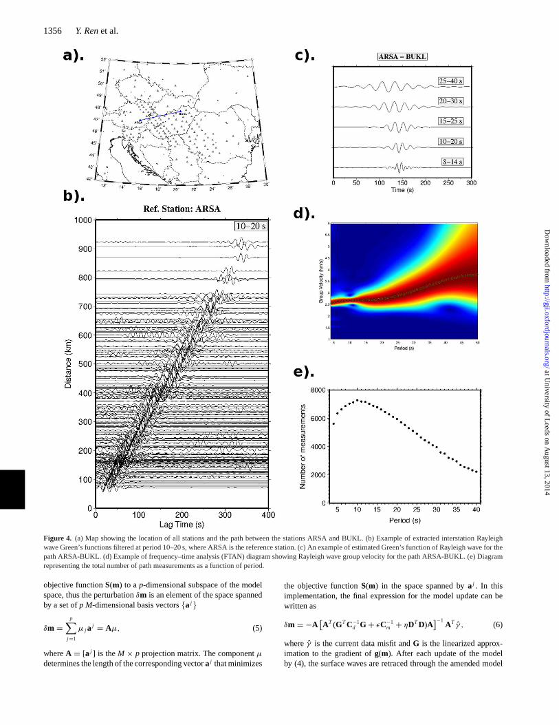
tf-PWS stacking technique yields much cleaner Green’s functions(Schimmelet al. 2010) (Fig. 3). Fig. 4(b) shows for example ourfinal estimated Rayleigh-wave Green’s functions propagating be-tween the station ARSA and all other stations, bandpass filteredbetween 10 and 20 s.

2.3 Group velocity dispersion measurements

We apply the frequency-time analysis (FTAN) multiple-filter tech-nique (Dziewonskiet al.1969) to measure the group velocity disper-sion curves in the period range 4–40 s from the estimated Rayleighwave Green’s function (Fig. 4d). We have studied over 13 354 in-terstation paths with a distance ranging from 20 to 1450 km. TheGaussian filter operator, used in the FTAN technique, is describedby exp[−α( f − fc)2/ f 2

c ], whereα determines the frequency reso-lution of the filter and fc is the centre frequency. Following Choet al. (2007), we have explored a wide range of values forα andfound that the best values for our study are between 5.0 and 20.0,depending on the interstation distance. Yanget al. (2007) pointedout that the stations must be separated by at least three wavelengthsto obtain a reliable dispersion curve measurement, and as such,each dispersion curve is used only for periods less than one third ofthe observed traveltime. The number of dispersion curve measure-ments used ranges from 2219 for 40 s period to 7267 for 10 s period.Fig. 4(e) shows the distribution of the number of measurements as afunction of the period. For the shortest and longest periods (T ≤ 5 sandT > 25 s), the number of measurements decreases significantlyas waveforms with poor signal-to-noise ratio are discarded.

3 G RO U P V E L O C I T Y T O M O G R A P H Y

We construct group velocity maps from the estimated Rayleighwave Green’s functions at periods from 4 to 40 s (with incrementof 1 s), using the non-linear 2-D tomographic inversion techniquedeveloped by Rawlinson & Sambridge (2003). Traveltimes throughthe 2-D model are computed using the fast marching algorithm ofSethian & Popovici (1999), in which a finite-difference method isused to solve the eikonal equation. This technique has some advan-tages over ray tracing methods as it is more stable, and successfullyfinds the first-arrival and diffraction paths in shadow zones. Theinversion procedure uses a gradient method based on the subspacetechnique (Kennettet al. 1988), where the minimization is carriedout simultaneously along several search directions that togetherspan a subspace of the model space (Rawlinson & Sambridge 2003,2004a,b). The technique has been successfully used for ambientnoise tomography in several regions (e.g. Arroucauet al. 2010;Saygin & Kennett 2012). We briefly describe the inversion proce-dure used here, but more details on the inversion technique can befound in Kennettet al. (1988), Williamson (1990) and Rawlinson& Sambridge (2003, 2004a,b).

3.1 Inversion method

The object of the tomographic inversion is to provide a model ofthe group velocity variation which best explains the interstationtraveltimes. This goal is formulated as the minimization of an ob-jective functionS(m) consisting of a data residual term and tworegularization terms:

S(m) =1

2

{

[g(m) − dobs]T C−1

d [g(m) − dobs]

+ ǫ(m − m0)T C−1

m (m − m0) + ηmT DT Dm}

(3)



Dow

nloaded from



Figure 3. Examples of estimated Rayleigh wave Green’s functions for paths between the station ARSA and SCP temporary stations (a) constructed using thelinear stacking technique (b) and using the tf-PWS stacking technique (c).

whereg(m) represents the predicted group traveltimes from themodelm, m0 is an initial estimate of the model,dobs is a vectorof the observed group traveltimes,Cd is the data covariance matrixfor which we assume a diagonal matrix with variances based ona uniform traveltime uncertainty of 2 s,Cm is thea priori modelcovariance matrix for which we assume a diagonal matrix withuniforma priori variances based on a model parameter uncertaintyof 0.3 km s−1, D is the derivative operator which has the role ofsmoothing the model,ǫ andη are respectively, the damping andsmoothing parameters. These choices of the variance estimates are

only approximate. The significant point is that we assume they areof uniform magnitude.

Following Rawlinson & Sambridge (2003), the minimization ofthe objective function is performed using an iterative approach toovercome the non-linearity ofg

mn+1 = mn + δm, (4)

whereδm is found iteratively using the subspace method. At eachiteration, the subspace method restricts the minimization of the



Dow

nloaded from


1356 Y. Renet al.

Figure 4. (a) Map showing the location of all stations and the path between the stations ARSA and BUKL. (b) Example of extracted interstation Rayleighwave Green’s functions filtered at period 10–20 s, where ARSA is the reference station. (c) An example of estimated Green’s function of Rayleigh wave for thepath ARSA-BUKL. (d) Example of frequency–time analysis (FTAN) diagram showing Rayleigh wave group velocity for the path ARSA-BUKL. (e) Diagramrepresenting the total number of path measurements as a function of period.

objective functionS(m) to ap-dimensional subspace of the modelspace, thus the perturbationδm is an element of the space spannedby a set ofp M-dimensional basis vectors{a j }

δm =p

∑

j =1

μ j a j = Aμ, (5)

whereA = [a j ] is theM × p projection matrix. The componentμ

determines the length of the corresponding vectora j that minimizes

the objective functionS(m) in the space spanned bya j . In thisimplementation, the final expression for the model update can bewritten as

δm = −A[

AT (GT C−1d G + ǫC−1

m + ηDT D)A]−1

AT γ , (6)

where ˆγ is the current data misfit andG is the linearized approx-imation to the gradient ofg(m). After each update of the modelby (4), the surface waves are retraced through the amended model



Dow

nloaded from



using the fast marching method, and then the termsA, γ and Gare re-evaluated. The final group velocity models presented in thispaper are obtained after eight iterations of the inversion at whichpoint the model update is small.

The region of interest in our study is 20◦ × 11◦ (Fig. 1). Weparametrized the area using a 0.2◦ × 0.2◦ grid of 5656 nodes wherevelocities are smoothly interpolated with the bicubic B-spline be-tween nodes to form a continuous group velocity field. The refer-ence velocity model used to damp the inversion (3) is the currentaverage velocity at the relevant period. We ran the inversion using arange of damping and smoothing parameters (0< ε, η < 5000) todetermine their optimal values. There is little significant differencebetween the various group velocity maps produced with differentregularization parameters; we present maps based on what we judgeto be optimum parameters (for dampingε = 10, for smoothingη = 60).

3.2 Resolution tests

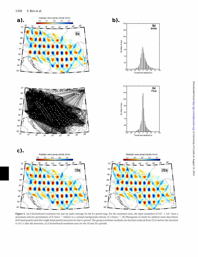
We performed checkerboard resolution tests to assess the reliabilityof the tomographic inversion. The input synthetic checkerboard ve-locity model consists of alternating cells (0.6◦ × 0.6◦) of oppositesign with a maximum velocity perturbation of 0.5 km s−1 relativeto the reference velocity. Between neighbouring anomalies, nullanomalies of similar size are defined. Synthetic group-velocity trav-eltime residuals were computed between the same station pairs usedin the observed data set using the fast marching method. Data noisewas not simulated in these tests. Fig. 5 shows the retrieved velocitymodels from these tests for periods of 6, 10 and 20 s. The checker-board tests (Fig. 5), show that our inversion can adequately resolvestructures as small as 60 km in most of the Carpathian–Pannonianregion, with some degradation or smearing of the recovered solu-tions near the edges of the station distribution map.

3.3 Depth sensitivity of Rayleigh group wave

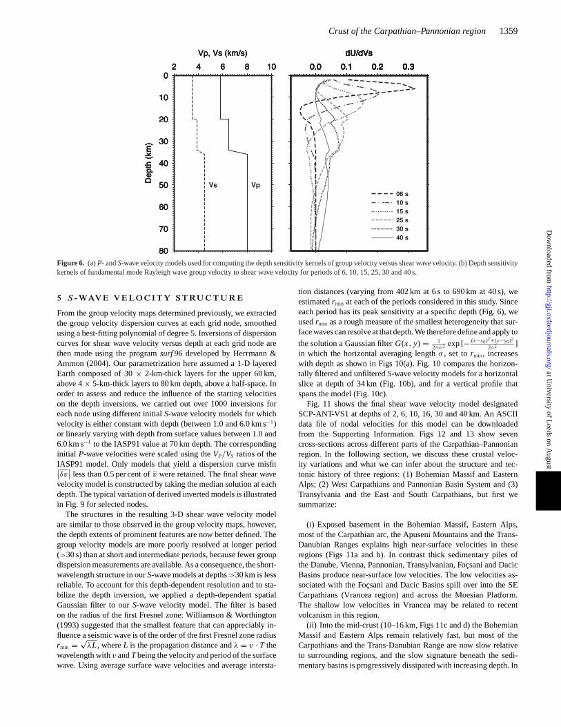
Surface waves at different periods are sensitive to structures at dif-ferent depths. Fig. 6 shows the depth dependence of shear wavevelocity sensitivity kernels for Rayleigh wave group velocity atperiods of 6, 10, 15, 25, 30 and 40 s, constructed using a modi-fied version of the AK135 model (Herrmann & Ammon 2004). Theshort period Rayleigh waves (4–10 s) are particularly sensitive to thesedimentary overburden and the shallower upper crust (to∼10 kmdepth). For the mid-period Rayleigh waves (10–20 s), the domi-nant sensitivity is at the mid-crustal depths (10–20 km); whereasthe longer period (20–30 s) Rayleigh waves are most sensitive tovelocities in the lower crust and uppermost mantle (20–40 km).Within our data set, only the Rayleigh waves at period 30–40 s con-strain the deepest part of the lower crust and uppermost mantle(30–60 km).

4 G RO U P V E L O C I T Y M A P S

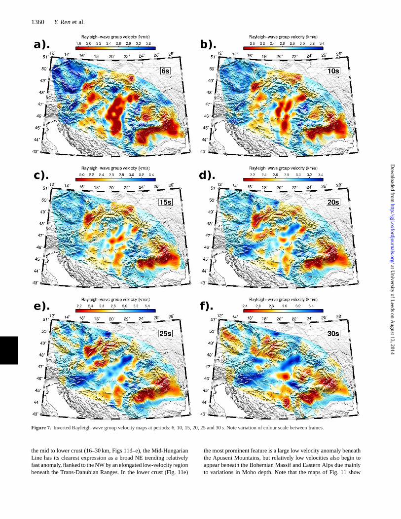
The Rayleigh-wave group velocity maps produced using our to-mographic analysis, for periods of 6, 10, 15, 20, 25 and 30 s, areshown in Fig. 7. The group velocity maps at short periods (e.g. 6 and10 s maps in Fig. 7) show coherent high and low velocity features,which accord well with surface tectonic features. At 6 s, high veloc-ities are dominant where crystalline rocks outcrop. High velocitiesare observed beneath the Bohemian Massif and the Eastern Alps

on Rayleigh-wave group velocity maps for periods up to about 20 s(Figs 7a–d); whereas the Transdanubian Ranges northwest of theMid-Hungarian line and the West Carpathians present high veloci-ties only to about 10 s periods. For the Southeast Carpathians highvelocities are not present even at 6 s, although high velocities areobserved further north in the East Carpathians and further west inthe South Carpathians, most clearly in the period range 4–8 s (see6 s map in Fig. 7). However, the low velocity features which domi-nate the southern half of the South Carpathians around the oroclineare clearly affected by the great sediment thicknesses in Dacic andFocsani Basins (Leever 2007).

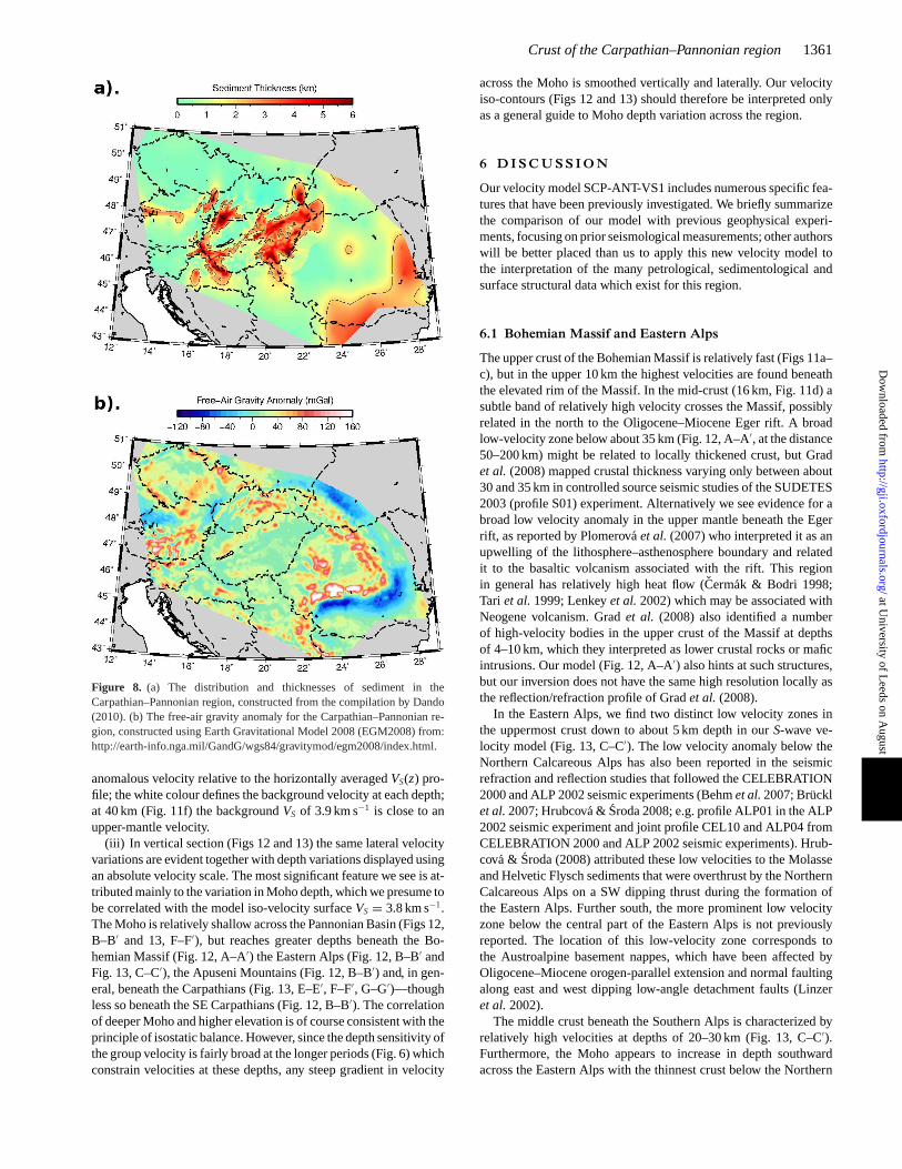
The relatively low group velocities at periods up to about 15 sreflect mainly thick sediments. All known sedimentary depocentresin the Carpathian–Pannonian region (Fig. 8a) are identified by thelow velocity regions in the 6 and 10 s group velocity maps (Figs 7aand b): the Bekes and Mako Basins below the Great HungarianPlain, Vienna and Danube Basins to the northwest, Drava Basin tothe southwest, Transylvanian Basin in western Romania, FocsaniBasin east of the Vrancea zone and finally the foredeep Dacic Basinof the Moesian platform (refer to Figs 12 and 13 for location ofthese basins). However, the sediment thicknesses of these differentbasins are highly variable. The broad low velocity zones below thePannonian Basins can be seen in our group velocity maps up to atleast 12 s period (Figs 7a and b), but some slow anomalies persisteven to 15 or 20 s period (Figs 7c and d). The Danube, Drava andTransylvanian basins are less deep and significantly low velocitiesare observed only to about 10 s. In contrast, low velocities persist to∼25 s for the Vienna and Focsani basins, as for the foredeep Dacicbasin of the Moesian platform. These basins are also associatedwith relatively large negative free-air gravity anomalies (Fig. 8b),unlike most of the intra-Carpathian basins which have near zerofree-air gravity anomalies.

At periods from 15 to 25 s (Figs 7c–e), group velocities becomeincreasingly sensitive to crustal thickness; lower velocities implythicker crust. The maps at these periods show low velocities be-neath almost the entire Carpathian range (West, East and South)along with relatively high free-air gravity anomalies (Fig. 8b). Thecontinuity of the low velocity anomaly below the East Carpathi-ans seems to be interrupted near the border between Ukraine andRomania by a localized fast anomaly but this is one of the morepoorly resolved locations in the solution (Fig. 5). The low veloci-ties along the South Carpathians persist to∼30 s period though theaxis of low velocities is clearly offset to the south from the topo-graphic axis of the South Carpathians. At periods from 30 to 40 s,we observe also the persistence of low velocities below the ApuseniMountains, and the southeastern corner of the Carpathians. Al-though, the low velocities of the Carpathians can be interpreted asthe signature of a deeper crustal root beneath the mountain belt,related to at least partial isostatic compensation, there is also astrong association in both West and East Carpathians with recentsurface volcanism and high temperatures at shallow depths (e.g.Central Slovakia Volcanic Field, CSVF, in the West Carpathians(Szabo et al. 1992) and the bend zone of the East Carpathians(Seghediet al.2004)).

At 20–25 s period, our group velocity maps (Figs 7d and e) showa distinctly SW–NE elongated high velocity zone traversing thePannonian region from the Eastern Alps in the SW, broadly alignedwith the Mid-Hungarian Line. These higher velocities might beinterpreted as a signature of crustal thinning. At greater periods(25–30 s) the Mid-Hungarian fast anomaly becomes more dominant,consistent with the idea of higher velocity mantle at shallower depthalong this trend.



Dow

nloaded from


1358 Y. Renet al.

Figure 5. (a) Checkerboard resolution test and ray path coverage for the 6 s period map. For the resolution tests, the input anomalies of 0.6◦ × 0.6◦ have amaximum velocity perturbation of 0.5 km s−1 relative to a constant background velocity of 2.6 km s−1. (b) Histograms of misfit for ambient noise data before(left-hand panels) and after (right-hand panels) inversion for the 6 s period. The group traveltime residuals rms has been reduced from 22.6 s before the inversionto 16.1 s after the inversion. (c) Checkerboard resolution tests for the 10 and 20 s periods.



Dow

nloaded from



Figure 6. (a)P- andS-wave velocity models used for computing the depth sensitivity kernels of group velocity versus shear wave velocity. (b) Depth sensitivitykernels of fundamental mode Rayleigh wave group velocity to shear wave velocity for periods of 6, 10, 15, 25, 30 and 40 s.

5 S - WAV E V E L O C I T Y S T RU C T U R E

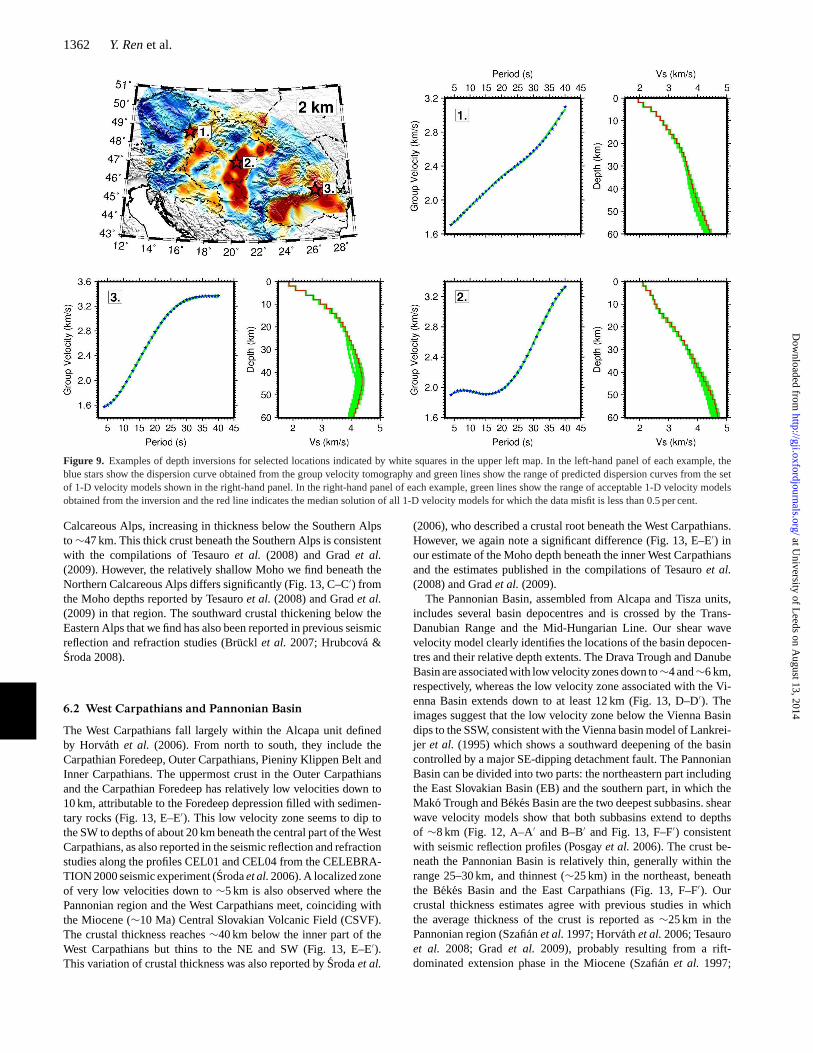
From the group velocity maps determined previously, we extractedthe group velocity dispersion curves at each grid node, smoothedusing a best-fitting polynomial of degree 5. Inversions of dispersioncurves for shear wave velocity versus depth at each grid node arethen made using the programsurf 96 developed by Herrmann &Ammon (2004). Our parametrization here assumed a 1-D layeredEarth composed of 30× 2-km-thick layers for the upper 60 km,above 4× 5-km-thick layers to 80 km depth, above a half-space. Inorder to assess and reduce the influence of the starting velocitieson the depth inversions, we carried out over 1000 inversions foreach node using different initialS-wave velocity models for whichvelocity is either constant with depth (between 1.0 and 6.0 km s−1)or linearly varying with depth from surface values between 1.0 and6.0 km s−1 to the IASP91 value at 70 km depth. The correspondinginitial P-wave velocities were scaled using theVP/VS ratios of theIASP91 model. Only models that yield a dispersion curve misfit∣

∣δv∣

∣ less than 0.5 per cent ofv were retained. The final shear wavevelocity model is constructed by taking the median solution at eachdepth. The typical variation of derived inverted models is illustratedin Fig. 9 for selected nodes.

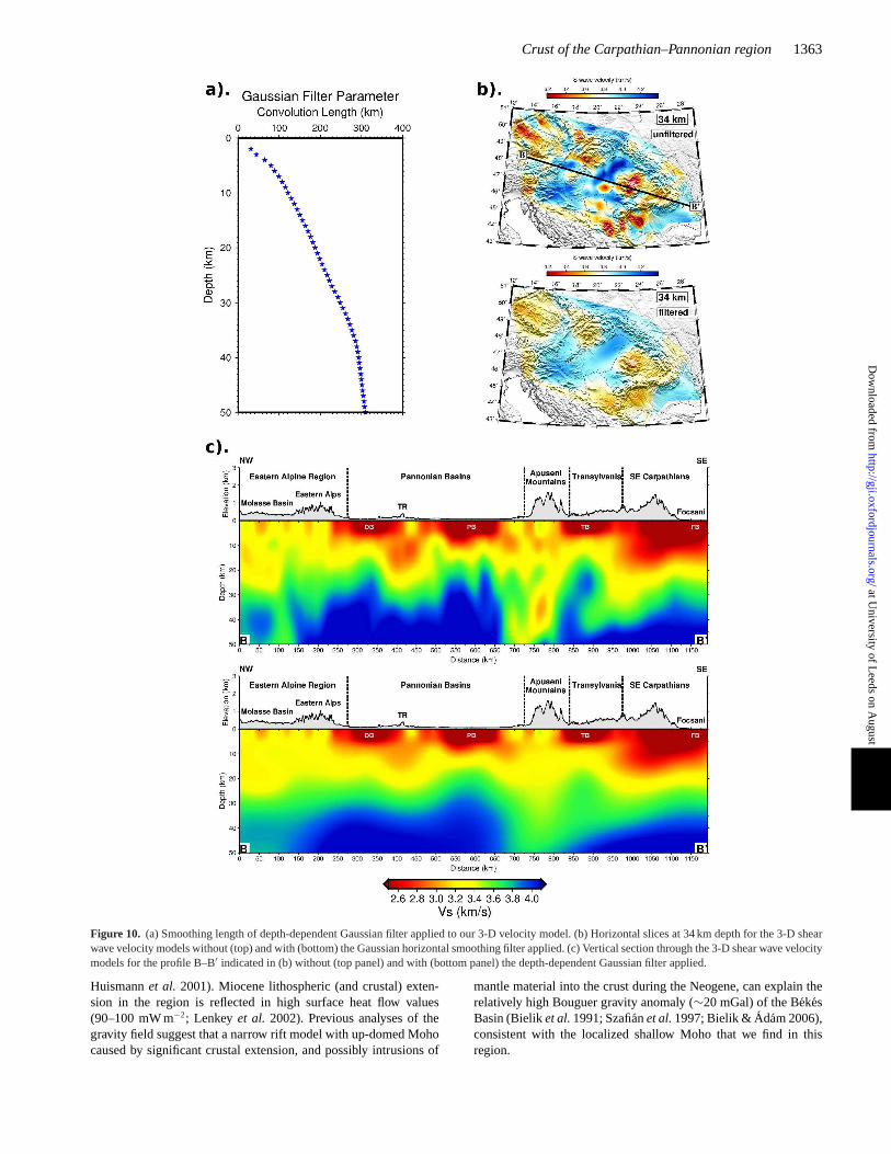
The structures in the resulting 3-D shear wave velocity modelare similar to those observed in the group velocity maps, however,the depth extents of prominent features are now better defined. Thegroup velocity models are more poorly resolved at longer period(>30 s) than at short and intermediate periods, because fewer groupdispersion measurements are available. As a consequence, the short-wavelength structure in ourS-wave models at depths>30 km is lessreliable. To account for this depth-dependent resolution and to sta-bilize the depth inversion, we applied a depth-dependent spatialGaussian filter to ourS-wave velocity model. The filter is basedon the radius of the first Fresnel zone: Williamson & Worthington(1993) suggested that the smallest feature that can appreciably in-fluence a seismic wave is of the order of the first Fresnel zone radiusrmin =

√λL, whereL is the propagation distance andλ = v · T the

wavelength withv andTbeing the velocity and period of the surfacewave. Using average surface wave velocities and average intersta-

tion distances (varying from 402 km at 6 s to 690 km at 40 s), weestimatedrmin at each of the periods considered in this study. Sinceeach period has its peak sensitivity at a specific depth (Fig. 6), weusedrmin as a rough measure of the smallest heterogeneity that sur-face waves can resolve at that depth. We therefore define and apply to

the solution a Gaussian filterG(x, y) = 12πσ2 exp [− (x−x0)2+(y−y0)2

2σ2 ]in which the horizontal averaging lengthσ , set tormin, increaseswith depth as shown in Figs 10(a). Fig. 10 compares the horizon-tally filtered and unfilteredS-wave velocity models for a horizontalslice at depth of 34 km (Fig. 10b), and for a vertical profile thatspans the model (Fig. 10c).

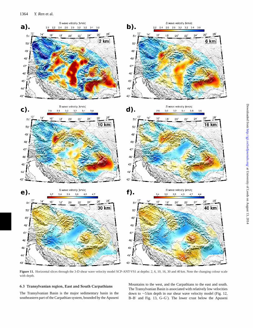
Fig. 11 shows the final shear wave velocity model designatedSCP-ANT-VS1 at depths of 2, 6, 10, 16, 30 and 40 km. An ASCIIdata file of nodal velocities for this model can be downloadedfrom the Supporting Information. Figs 12 and 13 show sevencross-sections across different parts of the Carpathian–Pannonianregion. In the following section, we discuss these crustal veloc-ity variations and what we can infer about the structure and tec-tonic history of three regions: (1) Bohemian Massif and EasternAlps; (2) West Carpathians and Pannonian Basin System and (3)Transylvania and the East and South Carpathians, but first wesummarize:

(i) Exposed basement in the Bohemian Massif, Eastern Alps,most of the Carpathian arc, the Apuseni Mountains and the Trans-Danubian Ranges explains high near-surface velocities in theseregions (Figs 11a and b). In contrast thick sedimentary piles ofthe Danube, Vienna, Pannonian, Transylvanian, Focsani and DacicBasins produce near-surface low velocities. The low velocities as-sociated with the Focsani and Dacic Basins spill over into the SECarpathians (Vrancea region) and across the Moesian Platform.The shallow low velocities in Vrancea may be related to recentvolcanism in this region.

(ii) Into the mid-crust (10–16 km, Figs 11c and d) the BohemianMassif and Eastern Alps remain relatively fast, but most of theCarpathians and the Trans-Danubian Range are now slow relativeto surrounding regions, and the slow signature beneath the sedi-mentary basins is progressively dissipated with increasing depth. In



Dow

nloaded from


1360 Y. Renet al.

Figure 7. Inverted Rayleigh-wave group velocity maps at periods: 6, 10, 15, 20, 25 and 30 s. Note variation of colour scale between frames.

the mid to lower crust (16–30 km, Figs 11d–e), the Mid-HungarianLine has its clearest expression as a broad NE trending relativelyfast anomaly, flanked to the NW by an elongated low-velocity regionbeneath the Trans-Danubian Ranges. In the lower crust (Fig. 11e)

the most prominent feature is a large low velocity anomaly beneaththe Apuseni Mountains, but relatively low velocities also begin toappear beneath the Bohemian Massif and Eastern Alps due mainlyto variations in Moho depth. Note that the maps of Fig. 11 show



Dow

nloaded from



Figure 8. (a) The distribution and thicknesses of sediment in theCarpathian–Pannonian region, constructed from the compilation by Dando(2010). (b) The free-air gravity anomaly for the Carpathian–Pannonian re-gion, constructed using Earth Gravitational Model 2008 (EGM2008) from:http://earth-info.nga.mil/GandG/wgs84/gravitymod/egm2008/index.html.

anomalous velocity relative to the horizontally averagedVS(z) pro-file; the white colour defines the background velocity at each depth;at 40 km (Fig. 11f) the backgroundVS of 3.9 km s−1 is close to anupper-mantle velocity.

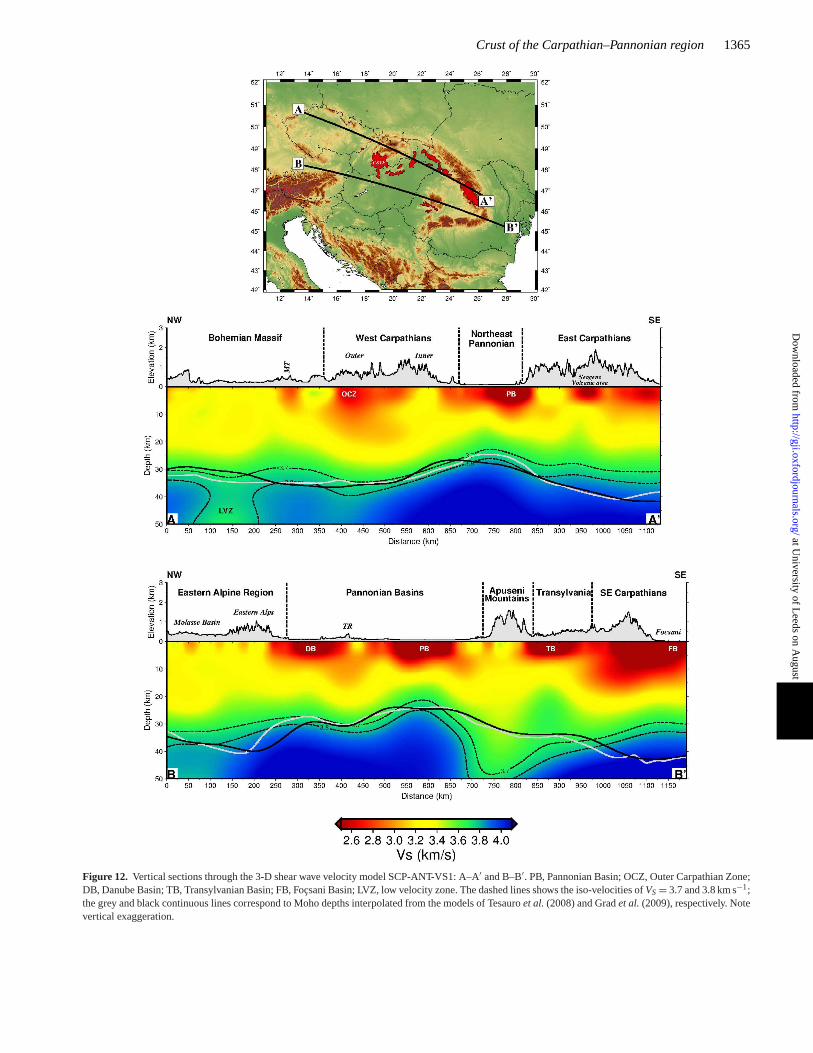
(iii) In vertical section (Figs 12 and 13) the same lateral velocityvariations are evident together with depth variations displayed usingan absolute velocity scale. The most significant feature we see is at-tributed mainly to the variation in Moho depth, which we presume tobe correlated with the model iso-velocity surfaceVS = 3.8 km s−1.The Moho is relatively shallow across the Pannonian Basin (Figs 12,B–B′ and 13, F–F′), but reaches greater depths beneath the Bo-hemian Massif (Fig. 12, A–A′) the Eastern Alps (Fig. 12, B–B′ andFig. 13, C–C′), the Apuseni Mountains (Fig. 12, B–B′) and, in gen-eral, beneath the Carpathians (Fig. 13, E–E′, F–F′, G–G′)—thoughless so beneath the SE Carpathians (Fig. 12, B–B′). The correlationof deeper Moho and higher elevation is of course consistent with theprinciple of isostatic balance. However, since the depth sensitivity ofthe group velocity is fairly broad at the longer periods (Fig. 6) whichconstrain velocities at these depths, any steep gradient in velocity

across the Moho is smoothed vertically and laterally. Our velocityiso-contours (Figs 12 and 13) should therefore be interpreted onlyas a general guide to Moho depth variation across the region.

6 D I S C U S S I O N

Our velocity model SCP-ANT-VS1 includes numerous specific fea-tures that have been previously investigated. We briefly summarizethe comparison of our model with previous geophysical experi-ments, focusing on prior seismological measurements; other authorswill be better placed than us to apply this new velocity model tothe interpretation of the many petrological, sedimentological andsurface structural data which exist for this region.

6.1 Bohemian Massif and Eastern Alps

The upper crust of the Bohemian Massif is relatively fast (Figs 11a–c), but in the upper 10 km the highest velocities are found beneaththe elevated rim of the Massif. In the mid-crust (16 km, Fig. 11d) asubtle band of relatively high velocity crosses the Massif, possiblyrelated in the north to the Oligocene–Miocene Eger rift. A broadlow-velocity zone below about 35 km (Fig. 12, A–A′, at the distance50–200 km) might be related to locally thickened crust, but Gradet al. (2008) mapped crustal thickness varying only between about30 and 35 km in controlled source seismic studies of the SUDETES2003 (profile S01) experiment. Alternatively we see evidence for abroad low velocity anomaly in the upper mantle beneath the Egerrift, as reported by Plomerovaet al. (2007) who interpreted it as anupwelling of the lithosphere–asthenosphere boundary and relatedit to the basaltic volcanism associated with the rift. This regionin general has relatively high heat flow (Cermak & Bodri 1998;Tari et al.1999; Lenkeyet al.2002) which may be associated withNeogene volcanism. Gradet al. (2008) also identified a numberof high-velocity bodies in the upper crust of the Massif at depthsof 4–10 km, which they interpreted as lower crustal rocks or maficintrusions. Our model (Fig. 12, A–A′) also hints at such structures,but our inversion does not have the same high resolution locally asthe reflection/refraction profile of Gradet al. (2008).

In the Eastern Alps, we find two distinct low velocity zones inthe uppermost crust down to about 5 km depth in ourS-wave ve-locity model (Fig. 13, C–C′). The low velocity anomaly below theNorthern Calcareous Alps has also been reported in the seismicrefraction and reflection studies that followed the CELEBRATION2000 and ALP 2002 seismic experiments (Behmet al.2007; Brucklet al.2007; Hrubcova & Sroda 2008; e.g. profile ALP01 in the ALP2002 seismic experiment and joint profile CEL10 and ALP04 fromCELEBRATION 2000 and ALP 2002 seismic experiments). Hrub-cova & Sroda (2008) attributed these low velocities to the Molasseand Helvetic Flysch sediments that were overthrust by the NorthernCalcareous Alps on a SW dipping thrust during the formation ofthe Eastern Alps. Further south, the more prominent low velocityzone below the central part of the Eastern Alps is not previouslyreported. The location of this low-velocity zone corresponds tothe Austroalpine basement nappes, which have been affected byOligocene–Miocene orogen-parallel extension and normal faultingalong east and west dipping low-angle detachment faults (Linzeret al.2002).

The middle crust beneath the Southern Alps is characterized byrelatively high velocities at depths of 20–30 km (Fig. 13, C–C′).Furthermore, the Moho appears to increase in depth southwardacross the Eastern Alps with the thinnest crust below the Northern



Dow

nloaded from


1362 Y. Renet al.

Figure 9. Examples of depth inversions for selected locations indicated by white squares in the upper left map. In the left-hand panel of each example, theblue stars show the dispersion curve obtained from the group velocity tomography and green lines show the range of predicted dispersion curves from the setof 1-D velocity models shown in the right-hand panel. In the right-hand panel of each example, green lines show the range of acceptable 1-D velocity modelsobtained from the inversion and the red line indicates the median solution of all 1-D velocity models for which the data misfit is less than 0.5 per cent.

Calcareous Alps, increasing in thickness below the Southern Alpsto ∼47 km. This thick crust beneath the Southern Alps is consistentwith the compilations of Tesauroet al. (2008) and Gradet al.(2009). However, the relatively shallow Moho we find beneath theNorthern Calcareous Alps differs significantly (Fig. 13, C–C′) fromthe Moho depths reported by Tesauroet al. (2008) and Gradet al.(2009) in that region. The southward crustal thickening below theEastern Alps that we find has also been reported in previous seismicreflection and refraction studies (Bruckl et al. 2007; Hrubcova &Sroda 2008).

6.2 West Carpathians and Pannonian Basin

The West Carpathians fall largely within the Alcapa unit definedby Horvath et al. (2006). From north to south, they include theCarpathian Foredeep, Outer Carpathians, Pieniny Klippen Belt andInner Carpathians. The uppermost crust in the Outer Carpathiansand the Carpathian Foredeep has relatively low velocities down to10 km, attributable to the Foredeep depression filled with sedimen-tary rocks (Fig. 13, E–E′). This low velocity zone seems to dip tothe SW to depths of about 20 km beneath the central part of the WestCarpathians, as also reported in the seismic reflection and refractionstudies along the profiles CEL01 and CEL04 from the CELEBRA-TION 2000 seismic experiment (Srodaet al.2006). A localized zoneof very low velocities down to∼5 km is also observed where thePannonian region and the West Carpathians meet, coinciding withthe Miocene (∼10 Ma) Central Slovakian Volcanic Field (CSVF).The crustal thickness reaches∼40 km below the inner part of theWest Carpathians but thins to the NE and SW (Fig. 13, E–E′).This variation of crustal thickness was also reported bySrodaet al.

(2006), who described a crustal root beneath the West Carpathians.However, we again note a significant difference (Fig. 13, E–E′) inour estimate of the Moho depth beneath the inner West Carpathiansand the estimates published in the compilations of Tesauroet al.(2008) and Gradet al. (2009).

The Pannonian Basin, assembled from Alcapa and Tisza units,includes several basin depocentres and is crossed by the Trans-Danubian Range and the Mid-Hungarian Line. Our shear wavevelocity model clearly identifies the locations of the basin depocen-tres and their relative depth extents. The Drava Trough and DanubeBasin are associated with low velocity zones down to∼4 and∼6 km,respectively, whereas the low velocity zone associated with the Vi-enna Basin extends down to at least 12 km (Fig. 13, D–D′). Theimages suggest that the low velocity zone below the Vienna Basindips to the SSW, consistent with the Vienna basin model of Lankrei-jer et al. (1995) which shows a southward deepening of the basincontrolled by a major SE-dipping detachment fault. The PannonianBasin can be divided into two parts: the northeastern part includingthe East Slovakian Basin (EB) and the southern part, in which theMako Trough and Bekes Basin are the two deepest subbasins. shearwave velocity models show that both subbasins extend to depthsof ∼8 km (Fig. 12, A–A′ and B–B′ and Fig. 13, F–F′) consistentwith seismic reflection profiles (Posgayet al. 2006). The crust be-neath the Pannonian Basin is relatively thin, generally within therange 25–30 km, and thinnest (∼25 km) in the northeast, beneaththe Bekes Basin and the East Carpathians (Fig. 13, F–F′). Ourcrustal thickness estimates agree with previous studies in whichthe average thickness of the crust is reported as∼25 km in thePannonian region (Szafianet al.1997; Horvathet al.2006; Tesauroet al. 2008; Gradet al. 2009), probably resulting from a rift-dominated extension phase in the Miocene (Szafian et al. 1997;



Dow

nloaded from



Figure 10. (a) Smoothing length of depth-dependent Gaussian filter applied to our 3-D velocity model. (b) Horizontal slices at 34 km depth for the 3-D shearwave velocity models without (top) and with (bottom) the Gaussian horizontal smoothing filter applied. (c) Vertical section through the 3-D shear wave velocitymodels for the profile B–B′ indicated in (b) without (top panel) and with (bottom panel) the depth-dependent Gaussian filter applied.

Huismannet al. 2001). Miocene lithospheric (and crustal) exten-sion in the region is reflected in high surface heat flow values(90–100 mW m−2; Lenkey et al. 2002). Previous analyses of thegravity field suggest that a narrow rift model with up-domed Mohocaused by significant crustal extension, and possibly intrusions of

mantle material into the crust during the Neogene, can explain therelatively high Bouguer gravity anomaly (∼20 mGal) of the BekesBasin (Bieliket al.1991; Szafianet al.1997; Bielik & Adam 2006),consistent with the localized shallow Moho that we find in thisregion.



Dow

nloaded from


1364 Y. Renet al.

Figure 11. Horizontal slices through the 3-D shear wave velocity model SCP-ANT-VS1 at depths: 2, 6, 10, 16, 30 and 40 km. Note the changing colour scalewith depth.

6.3 Transylvanian region, East and South Carpathians

The Transylvanian Basin is the major sedimentary basin in thesoutheastern part of the Carpathian system, bounded by the Apuseni

Mountains to the west, and the Carpathians to the east and south.The Transylvanian Basin is associated with relatively low velocitiesdown to∼5 km depth in our shear wave velocity model (Fig. 12,B–B′ and Fig. 13, G–G′). The lower crust below the Apuseni



Dow

nloaded from



Figure 12. Vertical sections through the 3-D shear wave velocity model SCP-ANT-VS1: A–A′ and B–B′. PB, Pannonian Basin; OCZ, Outer Carpathian Zone;DB, Danube Basin; TB, Transylvanian Basin; FB, Focsani Basin; LVZ, low velocity zone. The dashed lines shows the iso-velocities ofVS = 3.7 and 3.8 km s−1;the grey and black continuous lines correspond to Moho depths interpolated from the models of Tesauroet al.(2008) and Gradet al.(2009), respectively. Notevertical exaggeration.



Dow

nloaded from


1366 Y. Renet al.

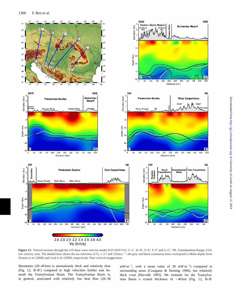
Figure 13. Vertical sections through the 3-D shear wave velocity model SCP-ANT-VS1: C–C′, D–D′, E–E′, F–F′ and G–G′. TR, Transdanubian Range; LVZ,low velocity zone. The dashed lines shows the iso-velocities ofVS = 3.7 and 3.8 km s−1; the grey and black continuous lines correspond to Moho depths fromTesauroet al. (2008) and Gradet al. (2009), respectively. Note vertical exaggeration.

Mountains (20–40 km) is anomalously thick and relatively slow(Fig. 12, B–B′) compared to high velocities further east be-neath the Transylvanian Basin. The Transylvanian Basin is,in general, associated with relatively low heat flow (26–58

mW m−2, with a mean value of 38 mW m−2) compared tosurrounding areas (Cranganu & Deming 1996), but relativelythick crust (Horvath 1993). We estimate for the Transylva-nian Basin a crustal thickness of∼40 km (Fig. 12, B–B′



Dow

nloaded from



and Fig. 13, G–G′), somewhat less than the Moho depths(∼44–46 km) reported from the DRACULA I+DACIA PLANseismic reflection studies by Fillerupet al. (2010). Tesauroet al.(2008) and Gradet al. (2009), however, estimated a Moho depthof about 30–35 km for the Transylvanian Basin regions. Further-more both of those compilations have missed the thick crust we findbeneath the Apuseni Mountains and conversely they find greatercrustal thickness than we find beneath the SE Carpathians and theFocsani Basin where crustal thickness decreases systematically to30–35 km (Fig. 12, B–B′).

In the East Carpathians, the Neogene volcanic region northof the Vrancea Zone, is associated with low velocities down to∼6 km depth (Fig. 12, A–A′). To the southeast of the Carpathi-ans, a broad low velocity region is attributable to the foredeepzone of the Focsani Basin with low velocities down to 10–15 km(Fig. 12, B–B′), consistent with the 15 km deep Focsani basementinferred from the VRANCEA 2001 seismic line (Hauseret al.2007). Furthermore, the section B–B′ (Fig. 12) suggests that thelow velocities of the basin dip beneath the East Carpathians tothe west, as if Focsani sediments underthrust the Carpathian oro-gen. The upper crust of the South Carpathians is associated witha localized high velocity anomaly, which is near vertical in theupper 10 km (Fig. 13, G–G′) and contrasts strongly with the shallow(≃10 km) low velocities of the Moesian Platform (correspondingto the Dacic foredeep basin) on one side and the TransylvanianBasin on the other side. This fast structure appears coherent rightthrough the crust, dipping to the NE beneath the TransylvanianBasin.

The East Carpathian crustal thickness increases systematically tothe north from∼32 km (Fig. 12, A–A′, B–B′) to ∼35 km (Fig. 13,F–F′, G–G′), but in general appears thinner than the estimates(∼40 km) of Tesauroet al. (2008) and Gradet al. (2009). In ourmodel relatively thin crust (∼32 km) is found below the contactzone between the East Carpathians and Focsani Basin, whereasmeasurements from the VRANCEA 2001 seismic refraction line(Hauseret al.2007) and the DRACULA I+DACIA PLAN seismicreflection profile (Fillerupet al. 2010) suggest a crustal thicknessof ∼42–45 km below the Focsani Basin, thinning towards the NWto ∼31–33 km in the Vrancea Zone of the SE Carpathians. Finally,the thicker crust of the South Carpathians (∼40 km; Fig. 13, G–G′) is broadly consistent with the crustal root suggested by Szafian& Horvath (2006) to explain the observed low Bouguer gravityanomalies (≤−100 mgal) in the South Carpathians.

7 C O N C LU S I O N S

A new high-resolution shear wave velocity model for the crust of theCarpathian–Pannonian region has been obtained using tomographicinversion of Rayleigh waves at periods 4–40 s retrieved from am-bient seismic noise analysis. Our group velocity maps show goodquantitative agreement with known geological features. We demon-strate that Rayleigh-wave dispersion curves obtained from ambientnoise correlation at periods as short as 4–8 s can image very wellthe sedimentary basins and their depth extents. High topographicregions are associated with high group velocities at short periods (4–8 s) corresponding to near-surface crystalline rocks and low groupvelocities at mid-periods (15–22 s) consistent with the thicker crustrequired for isostatic compensation. Long period group velocitymaps (>25 s) show high velocities in the Pannonian Basin, consis-tent with the crustal thinning which occurred during basin extension.Our shear wave velocity model SCP-ANT-VS1 obtained from the

inversion of the group velocity maps has been compared, where pos-sible, with previous geophysical investigations. In general our newmodel is validated by these comparisons, but some intriguing dif-ferences are found, notably in relation to crustal thickness estimatesbeneath the Apuseni Mountains and the Southeast Carpathians. Tosummarize the main features of the model:

(i) At shallow depths (<10 km), high topographic regions likethe Bohemian Massif, Eastern Alps, most of the Carpathian arc, theApuseni Mountains and the Trans-Danubian Ranges are associatedwith relatively high velocities, whereas sedimentary domains likethe Danube, Vienna, Pannonian, Transylvanian, Focsani and DacicBasins have low velocities. The low velocities associated with theFocsani and Dacic Basins seem to intrude below the SE Carpathians(Vrancea region) and across the Moesian Platform.

(ii) The middle crust (10–16 km) beneath the Bohemian Massifand Eastern Alps is relatively fast, but most of the Carpathiansand the Trans-Danubian Range are slow at these depths relative tosurrounding regions, and the slow signature beneath the sedimentarybasins is progressively dissipated with depth.

(iii) In the mid to lower crust (16–34 km), the Mid-HungarianLine is associated with a broad NE trending relatively fast anomaly,flanked to the NW by an elongated region of low velocities beneaththe Trans-Danubian Ranges.

(iv) At depths of 30–40 km, relatively low velocities appear be-neath the Bohemian Massif and Eastern Alps but the most prominentfeature is a large low velocity anomaly interpreted as anomalouslythick crust beneath the Apuseni Mountains. Most of the Pannon-ian and Vienna Basin regions at these depths are relatively fast,presumably related to shallowing of the Moho.

(v) Our estimates of Moho depths, roughly based on the iso-velocity surfaceVS = 3.8 km s−1, are generally consistent with re-sults from previous studies and accord well with different tectonicfeatures though we find specific differences relative to two recentMoho compilations of Tesauroet al.(2008) and Gradet al.(2009).

A C K N OW L E D G E M E N T S

The South Carpathian Project was supported by NERC standardgrant NE/G005931/1. The seismological equipment used in theSCP network was provided by SEIS-UK as the NERC Geophys-ical Equipment Facility. The fieldwork for the SCP project was acollaborative project between the University of Leeds, UK, EotvosLorand Geophysical Institute (ELGI), Budapest, Hungary, NationalInstitute of Earth Physics (NIEP), Bucharest, Romania and the Seis-mological Survey of Serbia (SSS), Belgrade, Serbia. The SouthCarpathian Project Working Group includes: G. Houseman, G.Stuart, Y. Ren, B. Dando, P. Lorinczi, O. Gogus (University ofLeeds, UK); E. Hegedus, A. Kovacs, I. Torok, I. Laszlo, R. Csabafi(ELGI); C. Ionescu, M. Radulian, V. Raileanu, D. Tataru, B. Zaharia,F. Borleanu, C. Neagoe, G. Gainariu, D. Rau (NIEP);S. Radovanovic, V. Kovacevic, D. Valcic, S. Petrovic-Cacic, G.Krunic (SSS); A. Brisbourne, D. Hawthorn, V. Lane (SEIS-UK,Leicester University, UK). Data from permanent stations used inthis study were obtained from the GFZ, ORFEUS and IRIS seis-mological data archives with additional data from the Romanianregional network provided by NIEP. The authors thank N. Rawl-inson of Australian National University, for making available his2-D non-linear inversion code, M. Schimmel for his non-linearphase weighted stacking code and R. Herrmann of Saint Louis Uni-versity, St. Louis, Missouri, for providing his seismological soft-ware package, which is used for the dispersion curve inversion.



Dow

nloaded from


1368 Y. Renet al.

Most figures were made using GMT software (Wessel & Smith1998). We thank Nick Rawlinson and an anonymous reviewerfor their valuable comments/suggestions which improved thismanuscript.

R E F E R E N C E S

Arroucau, P., Rawlinson, N. & Sambridge, M., 2010. New insight intoCainozoic sedimentary basins and Palaeozoic suture zones in southeastAustralia from ambient noise surface wave tomography,Geophys. Res.Lett.,37,L07303, doi:10.1029/2009GL041974.

Bassin, C., Laske, G. & Masters, G., 2000. Current limits of resolution forsurface wave tomography in North America,EOS, Trans. Am. geophys.Un., 81,F897.

Behm, M., Bruckl, E., Chwatal, W. & Thybo, H., 2007. Application of stack-ing and inversion techniques to 3D wide-angle reflection and refractionseismic data of the Eastern Alps,Geophys. J. Int.,170(1), 275–298.

Bensen, G.D., Ritzwoller, M.H., Barmin, M.P., Levshin, A.L., Lin, F.,Moschetti, M.P., Shapiro, N.M. & Yang, Y., 2007. Processing seismicambient noise data to obtain reliable broad.band surface wave dispersionmeasurements,Geophys. J. Int.,169,1239–1260.

Bielik, M., 1991. Density modelling of the Earth’s crust in the Intra-Carpathian basins, inGeodynamic Evolution of the Pannonian Basin,Vol. 62, pp. 123–132, ed. Karamata, S., Acad. Conf. Serbian Acad. Sci.Arts.

Bielik, M. & Ad am, A., 2006. Structure of the Lithosphere in the Carpathian-Pannonian Region, inThe Carpathians and Their Foreland: Geology andHydrocarbon Resources,pp. 699–706, eds Golonka, J. & Picha, F.J.,AAPG Memoir 84.

Bruckl, E. et al., 2003. ALP 2002 Seismic Experiment,Stud. Geophys.Geod.,47(3), 671–679.

Bruckl, E.et al., 2007. Crustal structure due to collisional and escape tec-tonics in the Eastern Alps region based on profiles Alp01 and Alp02from the ALP 2002 seismic experiment,J. geophys. Res.,112,B06308,doi:10.1029/2006JB004687.

Cermak, V. & Bodri, L., 1998. Heat flow map of Europe revisited, inMit-teilungen der Deutschen Geophysikalischen Gesellschaft,pp. 58–63, ed.Clauser, C., Sonderband II.

Cho, K.H., Herrmann, R.B., Ammon, C.J. & Lee, K., 2007. Imaging theUpper Crust of the Korean Peninsula by Surface-Wave Tomography,Bull.seism. Soc. Am.,97,198–207.

Cranganu, C. & Deming, D., 1996. Heat flow and hydrocarbon genera-tion in the Transylvanian basin, Romania,AAPG Bull.,80(10), 1641–1653.

Csontos, L. & Voros, A., 2004. Mesozoic plate reconstructions of theCarpathian region,Paleogeogr. Paleoclim. Paleoecol.,210,1–56.

Dando, B., 2010. Seismological structure of the Carpathian-Pannonian re-gion of central Europe,PhD thesis,School of Earth and Environment,University of Leeds.

Dando, B.D.E., Stuart, G.W., Houseman, G.A., Hegedus, E., Bruckl, E.& Radovanovic, S., 2011. Teleseismic tomography of the mantle in theCarpathian-Pannonian region of central Europe,Geophys. J. Int.,186,11–31.

Derode, A., Larose, E., Tanter, M., de Rosny, J., Tourim, A., Campillo,M. & Fink, M., 2003. Recovering the Green’s function from field-fieldcorrelations in an open scattering medium,J. acoust. Soc. Am.,113,2973–2976.

Dziewonski, A., Bloch, S. & Landisman, M., 1969. A technique for theanalysis of transient seismic signals,Bull. seism. Soc. Am.,59, 427–444.

Fillerup, M.A., Knapp, J.H., Knapp, C.C. & Raileanu, V., 2010. Mantleearthquakes in the absence of subduction? Continental delamination inthe Romanian Carpathians,Lithos,2(5), 333–340.

Gemmer, L. & Houseman, G.A., 2007. Convergence and extension driven bylithospheric gravitational instability: evolution of the Alpine-Carpathian-Pannonian system,Geophys. J. Int.,168,1276–1290.

Grad, M., Spicak, A., Keller, G.R., Guterch, A., Broz, M. & Hegedus, E.Working Group (incl. P.Sroda), 2003. SUDETES 2003 seismic experi-ment,Stud. Geophys. Geod.,47,681–689.

Grad, M., Guterch, A., Mazur, S., Keller, G.R.,Spicak, A., Hrubcova,P. & Geissler, W.H., 2008. Lithospheric structure of the Bohemian Mas-sif and adjacent Variscan belt in central Europe based on profile S01from the SUDETES 2003 experiment,J. geophys. Res.,113, B10304,doi:10.1029/2007JB005497.

Grad, M. & Tiira, T. ESC Working Group, 2009. The Moho depth map ofthe European Plate,Geophys. J. Int.,176(1), 279–292.

Guterch, A.et al., 2003. CELEBRATION 2000 seismic experiment,Stud.Geophys. Geod.,47,659–669.

Hauser, F., Raileanu, V., Fielitz, W., Dinu, C., Landes, M., Bala, A.& Prodehl, C., 2007. Seismic crustal structure between the Tran-sylvanian Basin and the Black Sea, Romania,Tectonophysics,430,1–25.

Herrmann, R.B. & Ammon, C.J., 2004.Computer programs inseismology—3.30: GSAC—generic seismic application coding,Availableat: http://www.eas.slu.edu/eqc/eqccps.html (last accessed 2013).

Horvath, F., 1993. Towards a mechanical model for the formation of thePannonian basin,Tectonophysics,226,333–357.

Horvath, F., Bada, G., Szafian, P., Tari, G.,Adam, A. & Cloetingh, S.,2006. Formation and deformation of the Pannonian Basin: constraintsfrom observational data, inEuropean Lithosphere Dynamics,Vol. 32pp. 191–206, eds Gee, D. & Stephensen, R., Geological Society ofLondon Memoirs, Geological Society of London.

Houseman, G.A. & Gemmer, L., 2007. Intra-orogenic extension driven bygravitational instability: Carpathian-Pannonian orogeny,Geology,35(12),1135–1138.

Hrubcova, P. & Sroda, P. CELEBRATION 2000 Working Group, 2008.Crustal structure at the easternmost termination of the Variscan belt basedon CELEBRATION 2000 and ALP 2002 data,Tectonophysics,460,55–75.

Huismans, R.S., Podladchikov, Y.Y. & Cloetingh, S., 2001. Dynamic mod-eling of the transition from passive to active rifting, application to thePannonian basin,Tectonics,20(6), 1021–1039.

Ivan, M., 2011. Crustal thickness in Vrancea area, Romania fromS to Pconverted waves,J. Seismol.,15,317–328.

Kang, T.S. & Shin, J.S., 2006. Surface-wave tomography from ambientseismic noise of accelerograph networks in southern Korea,Geophys.Res. Lett.,33,L17303, doi:10.1029/2006GL027044.

Kennett, B.L.N., Sambridge, M. & Williamson, P.R., 1988. Subspace meth-ods for large scale inverse problems involving multiple parameter classes,Geophys. J. Int.,94,237–247.

Kovacs, I. & Haas, J., 2011. Displaced South Alpine and Dinaridic elementsin the mid-Hungarian zone,Central Eur. Geol.,53(2), 135–164.

Lankreijer, A., Kovacs, M., Cloetingh, S., Pitonak, P., Hloska, M. & Bier-mann, C., 1995. Quantitative subsidence analysis and forward modellingof the Vienna and Danube basins: thin-skinned versus thick-skinned ex-tension,Tectonophysics,252,433–451.

Larose, E., Derode, A., Corennec, D., Margerin, L. & Campillo, M., 2005.Passive retrieval of Rayleigh waves in disoredered elastic media,Phys.Rev. E.,72,046607, doi:10.113/PhysRevE.72.046607.

Leever, K.A., 2007. Foreland of the Romanian Carpathians Controls on lateorogenic sedimentary basin evolution and Paratethys paleogeography,PhD thesis,Vrije Universiteit Amsterdam.

Lenkey, L., Dovenyi, P., Horvath, F. & Cloetingh, S., 2002. Geothermics ofthe Pannonian basin and its bearing on the neotectonics,EGU StephenMueller Spec. Publ. Ser.,3, 29–41.

Li, H.Y., Su, W., Wang, C.Y. & Huang, Z.X., 2009. Ambient noise Rayleighwave tomography in western Sichuan and eastern Tibet,Earth planet. Sci.Lett.,282,201–211.

Lin, F.C., Ritzwoller, M.H., Townend, J., Savage, M. & Bannister, S., 2007.Ambient noise Rayleigh wave tomography of New Zealand,Geophys. J.Int., 72(2), 649–666.

Linzer, H.G., Decker, K., Peresson, H., DellMour, R. & Frisch, W., 2002.Balancing orogenic float of the Eastern Alps,Tectonophysics,354,211–237.



Dow

nloaded from

http://www.eas.slu.edu/eqc/eqccps.html



Martin, M., Ritter, J.R. & the CALIXTO working group, 2005. High-resolution teleseismic body-wave tomography beneath SE Romania—I.Implications for three-dimensional versus one-dimensional crustal cor-rection strategies with a new crustal velocity model,Geophys. J. Int.,162,448–460.

Marton, E. & Fodor, L., 1995. Combination of paleomagnetic and stressdata—a case study from North HungaryTectonophysics,242,99–114.

Moschetti, M.P., Ritzwoller, M.H. & Shapiro, N.M., 2007. Surface wavetomography of the western United States from ambient seismic noise:Rayleigh wave group velocity maps,Geochem. Geophys. Geosyst.,8,Q08010, doi:/10.1029/2007GC001655.

Patrascu, S., Panaiotu, C., Seclaman, M. & Panaiotu, C.E., 1994. Timingof rotational motion of Apuseni Mountains (Romania)—paleomagneticdata from Tertiary magmatic rocks,Tectonophysics,233(3/4), 163–176.

Plomerova, J., Achauer, U., Babuska, V. & Vecsey, L. BOHEMA workinggroup, 2007. Upper mantle beneath the Eger Rift (Central Europe): plumeor asthenosphere upwelling?,Geophys. J. Int.,169(2), 675–682.

Posgay, K., Bodoky, T., Hajnal, Z., Toth, T.M., Fancsik, T., Hegedus, E.,Kovacs, A.Cs. & Takac, E., 2006. Interpretation of subhorizontal crustalreflections by metamorphic and rheologic effects in the eastern part of thePannonian Basin,Geophys. J. Int.,167,187–203.

Rawlinson, N. & Sambridge, M., 2003. Seismic traveltime tomography ofthe crust and Lithosphere,Adv. Geophys.,46,81–198.

Rawlinson, N. & Sambridge, M., 2004a. Wave front evolution in stronglyheterogeneous layered media using the fast marching method,Geophys.J. Int.,156,631–647.

Rawlinson, N. & Sambridge, M., 2004b. Multiple reflection and transmis-sion phases in complex layered media using a multistage fast marchingmethod,Geophysics,69(5), 1338–1350.

Ren, Y. et al., 2012. Upper mantle structures beneath the Carpathian–Pannonian region: implications for geodynamics of the continental colli-sion,Earth planet. Sci. Lett.,349–350,139–152.

Royden, L.H., Horvath, F. & Burchfiel, B.C., 1982. Transform faulting,extension, and subduction in the Carpathian Pannonian Region,Geol.soc. Am. Bull.,93,717–725.

Sabra, K.G., Gerstoft, P., Roux, P., Kuperman, W.A. & Fehler, M.C., 2005.Surface wave tomography from microseisms in Southern California,Geo-phys. Res. Lett.,32,L14311, doi:10.1029/2005GL023155.

Saygin, E. & Kennett, B.L.N., 2012. Crustal structure of Australia fromambient seismic noise tomography,J. geophys. Res.,117, B01304,doi:10.1029/2011JB008403.

Schimmel, M., Stutzmann, E. & Gallart, J., 2010. Using instantaneous phasecoherence for signal extraction from ambient noise data at a local to aglobal scale,Geophys. J. Int.,184,494–506.

Seghedi, I.et al., 2004. Neogene “Quaternary magmatism and geodynamicsin the Carpathian” Pannonian region: a synthesis,Lithos,72(3–4), 117–146.

Sethian, J.A. & Popovici, A.M., 1999. 3-D traveltime computation using thefast marching method,Geophysics,64,516–523.

Shapiro, N.M., Campillo, M., Stehly, L. & Ritzwoller, M.H., 2005. High-resolution surface-wave tomography from ambient seismic noise,Science,307,1615–1618.

Snieder, R., 2004. Extracting the Green’s function from the correlation ofcoda waves: a derivation based on stationary phase,Phys. Rev. E,69,doi:10.1103/PhysRevE.69.046610.

Sroda, P.et al., 2006. Crustal and upper mantle structure of the WesternCarpathians from CELEBRATION 2000 profiles CEL01 and CEL04:seismic models and geological implications,Geophys. J. Int.,167,737–760.

Szabo, C., Harangi, S. & Csontos, L., 1992. Review of Neogene and Qua-ternary volcanism of the Carpathian-Pannonian region,Tectonophysics,208,243–256.

Szafian, P., Horvath, F. & Cloetingh, S.A.P.L., 1997. Gravity contraints onthe crustal structure and slab evolution along a Transcarpathian transect,Tectonophysics,272,233–248.

Szafian, P. & Horvath, F., 2006. Crustal structure in the Carpatho-Pannonianregion: insights from three-dimensional gravity modelling and their geo-dynamic significance,Int. J. Earth Sci.,95,50–67.

Tari, G., Dovenyi, P., Dunkl, I., Horvath, F., Lenkey, L., Stefanescu, M.,Szafian, P. & Toth, T., 1999. Lithospheric structure of the Pannonian basinderived from seismic, gravity and geothermal data,Geol. Soc. Lond., Spec.Publ.,156,215–250.

Tesauro, M., Kaban, M.K. & Cloetingh, S.A.P.L., 2008. EuCRUST-07: anew reference model for the European crust,Geophys. Res. Lett.,35,L05313, doi:10.1029/2007GL032244.

Wapenaar, K., 2004. Retrieving the elastodynamic Green’s function of anarbitrary inhomogeneous medium by cross correlation,Phys. Rev. Lett.,93,doi:10.1103/PhysRevLett.93.254301.

Weaver, R.L. & Lobkis, O.I., 2004. On the emergence of the Green’s functionin the correlations of a diffuse field,J. acoust. Soc. Am.,116,2731–2734.

Williamson, P.R., 1990. Tomographic inversion in reflection seismology,Geophys. J. Int.,100,255–274.

Williamson, P.R. & Worthington, M.H., 1993. Resolution limits in ray to-mography due to wave behavior: numerical experiments,Geophysics,58(5), 727–735.

Yang, Y., Ritzwoller, M.H., Levshin, A.L. & Shapiro, N.M., 2007. Ambientnoise Rayleigh wave tomography across Europe,Geophys. J. Int.,168,259–274.

Yao, H.J., van der Hilst, R.D. & de Hoop, M.V., 2006. Surface-wave arraytomography in SE Tibet from ambient seismic noise and two-stationanalysis—I. Phase velocity maps,Geophys. J. Int.,166,732–744.

S U P P O RT I N G I N F O R M AT I O N

Additional Supporting Information may be found in the online ver-sion of this article:

1. sup-0001-readme.txt2. sup-0002-SCP-ANT-VS1-0.2x0.2.dat3. sup-0003-SCP-ANT-VS1-0.05x0.05.dat(http://gji.oxfordjournals.org/lookup/suppl/doi:10.1093/gji/ggt316/-/DC1).

Please note: Oxford University Press is not responsible for the con-tent or functionality of any supporting materials supplied by theauthors. Any queries (other than missing material) should be di-rected to the corresponding author for the article.



Dow

nloaded from

http://gji.oxfordjournals.org/lookup/suppl/doi:10.1093/gji/ggt316/-/DC1

http://gji.oxfordjournals.org/lookup/suppl/doi:10.1093/gji/ggt316/-/DC1


Documents

core.ac.uk · Published by Oxford University Press on behalf of The Royal ... counter-clockwise rotation of ... crust and perhaps the upper few tens of kilometres