Embed Size (px)
Citation preview
Core Guide: Correlation Structures in LDA
1 | P a g e
Core Guide: Correlation Structures in Mixed
Effects Models for Longitudinal Data Analysis Part of a series addressing common issues in statistical and epidemiological design and analysis
Background
Longitudinal data, also commonly called repeated measures data, is defined as data collected on subjects,
or another unit of analysis (e.g., village) repeatedly over time. Whereas a time series usually includes a
long time series on a single (or small number of) sequences, repeated measures are typically measured
on a relatively large number of subjects over a more limited period of time. Measurements may be
approximately equally spaced, as may be the case in carefully controlled laboratory studies or clinical
trials, or unequally spaced, as may be the case in electronic health records (EHR) data where subjects are
measured when they happen to go to the doctor. Longitudinal data may also be balanced (i.e., having the
same number of measures on each subject) or unbalanced. Two primary methods of choice for analyzing
the relationship between an outcome and time (and other covariates) are generalized estimating
equations (GEE) and mixed-effects models (see Fitzmaurice, Laird, and Ware (2011)1 for detailed
background on each method). The current guide focuses on mixed-effects models, commonly referred to
succinctly as “mixed models”.
When data are repeatedly measured on the same subject over time, data collected on the same individual
are generally positively correlated with each other. For example, my weight today is generally correlated
with my weight one month from now, and my current risk of malaria is often correlated with my risk last
month, as well as last year at the same time (seasonal effect). However, we assume that data between
subjects is independent and uncorrelated, as would (ideally) be the case in an individually-randomized
controlled trial (RCT). In a cluster randomized controlled trial, however, we might have correlation among
individuals within the same cluster, as well as with repeated measures on the same individual over time.
See the recent review articles by Turner et al. for more information about cluster randomized trials.2,3
When data are positively correlated within individual, ignoring the correlation in the analysis (e.g., fitting
an ordinary least squares linear regression) will lead to inflated type I error rates for time-independent
variables (e.g., sex, race) because of underestimated standard errors and inflated type II error rates for
time-dependent variables (e.g., the time effect, certain biologic measurements and weight)..4
The purpose of the current core guide is to review modeling strategies of longitudinal person-level data
in the mixed effects modeling framework in order to account for within-person correlation. We
specifically focus on continuous outcomes, and discuss the modeling of different types of within-person
correlation structures through the use of random effects, the residual error terms and a combination of
both. We discuss different types of error structures and model data described in chapters 7 and 8 of
Core Guide: Correlation Structures in LDA
2 | P a g e
Fitzmaurice, Laird, and Ware (2011).1 Mixed effects models for non-Gaussian (e.g., binary) require
another set of methods, and interpretation of parameters is more complicated, so will be discussed in a
future core guide.
The Mixed-Effects Model
The mixed-effects model is useful for modeling outcome measurements in any type of grouped (i.e.,
correlated) data, whether those groups are schools, communities, families, or repeated measures within
subjects. In various types of literature, the mixed model has been formulated in both a two-stage and
one-stage manner.5 In this core guide, we focus on the more commonly used one-stage formulation
given by:
𝒀 = 𝑿𝜷 + 𝒁𝜸 + 𝜺; 𝜺~𝑵(𝟎, 𝑹), 𝜸~𝑵(𝟎, 𝑮) (1)
where 𝑿𝜷 is the “fixed-effects” part of the model, 𝒁𝜸 is the random effects part of the model, and
𝜺~𝑵(𝟎, 𝑹) is the residual error vector. 𝒀 “represents a vector of observed outcome data, 𝜷 is an
unknown vector of fixed-effects parameters with known design matrix 𝑿”, and “𝜸 is an unknown vector
of random-effects parameters with known design matrix 𝒁”.6 We use G to represent the variance-
covariance matrix of the random effects and R represents the variance-covariance matrix of the residual
errors. It follows that the total variance of 𝒀 is given by
𝑽 = 𝒁𝑮𝒁′ + 𝑹. (2)
What are the implications of specifying the correlation of repeated measurements on the same
individual by including the 𝜸 vector of random effects (i.e. and then specifying the structure of G)
and/or changing R? It is common for R to be specified as the identity matrix so that the residual errors
are assumed to be independent of each other. In this case, correlation of repeated measures on the
same individual can be accounted for by including random effects 𝜸 and by specifying a structure for G.
Another option is to not include random effects and to simply fit a structure on the R matrix to account
for within-person correlation. Some kinds of simple within-person correlation structures can be
specified using either formulation. For example, the commonly used ‘exchangeable’ (or compound
symmetry) correlation structure, in which the same correlation is assumed for all pairs of measurements
on the same person irrespective of their timing, can be modeled either by (1) including a random
intercept for each person (G =𝜎𝑏2I), or, (2) by not adding random intercepts but instead by setting R to
be a block diagonal matrix with the same covariance on the off diagonals.
The random effects can include a random intercept and any function of covariates of interest, e.g with a
random slope on time. Longitudinal models with both a random intercept and a random slope for time
induces a within-individual correlation matrix with correlations that decrease in magnitude the further
apart the measurements are on the same person—a common feature of longitudinal data. More
complex random effects structures—including adding polynomials for the time effect—are sometimes
used. More detail on random effects specification is given in the appendix.
Core Guide: Correlation Structures in LDA
3 | P a g e
When random effects are added to the model, fixed parameters are interpreted in terms of conditional
means. That is, the fixed-effects coefficients are interpreted in terms of changes in subject-specific
mean responses, rather than population-averaged mean response (e.g. as would be the case with the
GEE approach). However, as Fitzmaurice, Laird, and Ware (2011)1 show on page 404 of their book, in
the case of continuous outcomes (fitted with an identity link function) the population-averaged and
conditional models are the same (i.e., we can interpret the coefficients in both a population-level and
subject-specific manner). This is not the case for generalized linear mixed models (GLMMs), where the
conditional and population-averaged models can differ. This has implications for interpretation when
analyzing non-Gaussian data.
Commonly used parameter estimation methods are maxiumum likelihood estimation (MLE) and
restricted maximum likelihood estimation (REML). REML should be the estimation method of choice,
since the standard errors are biased downward with ML.7 When fitting regression models to
longitudinal data using either approach, it is important to remember that the fixed effects mean
structure is inherently linked to the covariance structure. Misspecified covariance structure leads to
biased estimates of coefficients in the model of the mean. Thus, it is important to properly specify the
covariance structure. Model selection procedures, such as the Akaike Information Criterion (AIC) or
likelihood ratio test, can be used to select the most appropriate covariance structure.
Conclusion
We have reviewed the theory behind the modeling of the covariance structure in linear mixed effects
models. The choice of modeling the random effects or simply modeling the R matrix depends on
whether one is interested in the covariance parameters themselves (modeling the random effects) or is
treating the covariance as a nuisance to model just in order to avoid bias in the mean parameters
(modeling the R matrix). The appendix contains detailed examples and code, including more discussion
on when to model the random effects or the R matrix. This core guide serves as an introduction to
modeling the covariance in longitudinal data analysis. For a more in-depth look at the topic, see for
example Fitzmaurice, Laird, and Ware (2011).1
Prepared by: John Gallis, MSc Reviewed by: Duke Global Health Institute | Research Design & Analysis Core Version: 1.1, last updated September 19, 2017
Core Guide: Correlation Structures in LDA
4 | P a g e
References
1. Fitzmaurice GM, Laird NM, Ware JH. Applied longitudinal analysis. 2nd ed. Hoboken, N.J.: Wiley; 2011.
2. Turner EL, Li F, Gallis JA, Prague M, Murray DM. Review of Recent Methodological Developments in Group-Randomized Trials: Part 1 - Design. Am J Public Health. 2017;107(6):907-915.
3. Turner EL, Prague M, Gallis JA, Li F, Murray DM. Review of Recent Methodological Developments in Group-Randomized Trials: Part 2 - Analysis. Am J Public Health. 2017;107(7):1078-1086.
4. Dunlop DD. Regression for longitudinal data: a bridge from least squares regression. The American Statistician. 1994;48:299+.
5. Singer JD. Using SAS PROC MIXED to fit multilevel models, hierarchical models, and individual growth models. J Educ Behav Stat. 1998;23(4):323-355.
6. SAS/STAT 9.2 user's guide. SAS Institute Cary, NC; 2008. 7. Littell RC, Milliken GA, Stroup WW, Wolfinger RD, Schabenberger O. SAS for mixed models. SAS
institute; 2007. 8. Wolfinger RD. Heterogeneous variance: covariance structures for repeated measures. J Agric
Biol Environ Stat. 1996:205-230. 9. Diggle P, Heagerty P, Liang K-Y, Zeger S. Analysis of longitudinal data. 2nd ed. Oxford ; New York:
Oxford University Press; 2002.
Core Guide: Correlation Structures in LDA
5 | P a g e
Appendix
Modeling correlation structures in common statistical software
In SAS PROC MIXED, which allows the user to fit linear mixed effects models with continuous outcomes,
we can model the the covariance structure of the random effects (G) using the RANDOM statement, and
we can model the covariance structure of of the errors (R) using the REPEATED statement (see equation
(1)). Hence, we can model the total variability in 𝒀 by specifying a structure on either the G or R matrix,
or both. In Stata, using the command mixed, the random effects are specified after ||, and the R matrix
is specified using the option residuals() after the random effects part of the model formulation.
We now move on to some examples, using data described and analyzed in chapters 7 and 8 of Fitzmaurice,
Laird, and Ware (2011).1
Example 1: Exploring random effects and residual correlation structures
For this first example, we use the exercise therapy trial data, as described on page 180 of Fitzmaurice,
Laird, and Ware (2011)1:
In this study, subjects were assigned to one of two weightlifting programs to increase muscle
strength. In the first program, hereafter referred to as treatment 1, the number of repetitions
of the exercises was increasaed as subjects became stronger. In the second program,
hereafter referred to as treatment 2, the number of repetitions was held constant but the
amount of weight was increased as subjects became stronger. Measurements of muscle
strength were taken at baseline and on days 2, 4, 6, 8, 10, and 12.
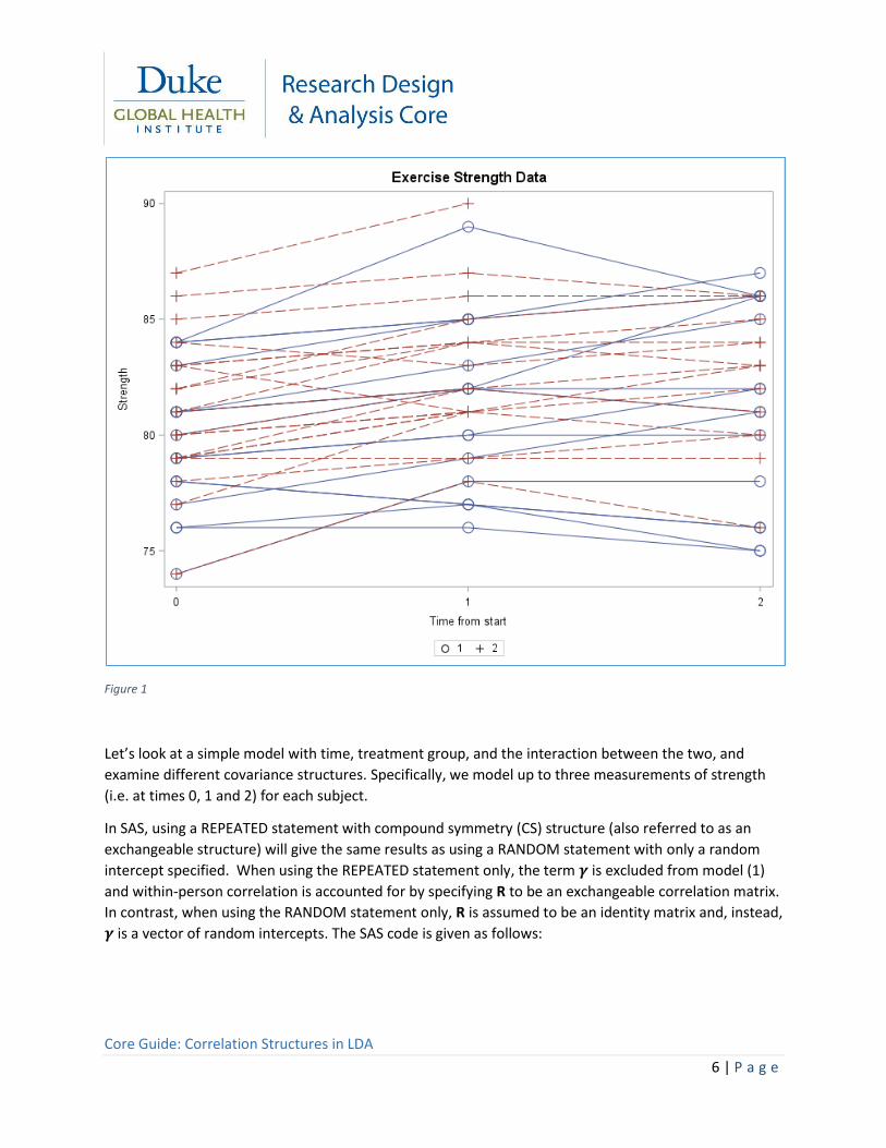
To simplify for this illustration, we only consider baseline, day 6, and day 12, referred to as time 0, 1,
and 2. The data on n=37 people are plotted in figure 1. It is difficult to get a good idea of the data from
the plot (often called a spaghetti plot), although it looks like a good number of people initially increase
in strength and then decline by time 2 (day 12). Some other features we notice are that at least one
subject is missing the final measurement (e.g. see the data shown in the the upper dashed red line).
Core Guide: Correlation Structures in LDA
6 | P a g e
Figure 1
Let’s look at a simple model with time, treatment group, and the interaction between the two, and
examine different covariance structures. Specifically, we model up to three measurements of strength
(i.e. at times 0, 1 and 2) for each subject.
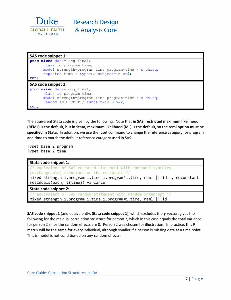
In SAS, using a REPEATED statement with compound symmetry (CS) structure (also referred to as an
exchangeable structure) will give the same results as using a RANDOM statement with only a random
intercept specified. When using the REPEATED statement only, the term 𝜸 is excluded from model (1)
and within-person correlation is accounted for by specifying R to be an exchangeable correlation matrix.
In contrast, when using the RANDOM statement only, R is assumed to be an identity matrix and, instead,
𝜸 is a vector of random intercepts. The SAS code is given as follows:
Core Guide: Correlation Structures in LDA
7 | P a g e
SAS code snippet 1: proc mixed data=long_final;
class id program time;
model strength=program time program*time / s chisq;
repeated time / type=CS subject=id R=2;
run;
SAS code snippet 2: proc mixed data=long_final;
class id program time;
model strength=program time program*time / s chisq;
random INTERCEPT / subject=id G V=2;
run;
The equivalent Stata code is given by the following. Note that in SAS, restricted maximum likelihood
(REML) is the default, but in Stata, maximum likelihood (ML) is the default, so the reml option must be
specified in Stata. In addition, we use the fvset command to change the reference category for program
and time to match the default reference category used in SAS.
fvset base 2 program fvset base 2 time
Stata code snippet 1: /* equivalent of SAS repeated statement with compound symmetry (exchangeable) structure on the residuals */ mixed strength i.program i.time i.program#i.time, reml || id: , noconstant residuals(exch, t(time)) variance
Stata code snippet 2: /* equivalent of SAS random statement with random intercept */ mixed strength i.program i.time i.program#i.time, reml || id:
SAS code snippet 1 (and equivalently, Stata code snippet 1), which excludes the 𝜸 vector, gives the
following for the residual correlation structure for person 2, which in this case equals the total variance
for person 2 since the random effects are 0. Person 2 was chosen for illustration. In practice, this R
matrix will be the same for every individual, although smaller if a person is missing data at a time point.
This is model is not conditioned on any random effects.
Core Guide: Correlation Structures in LDA
8 | P a g e
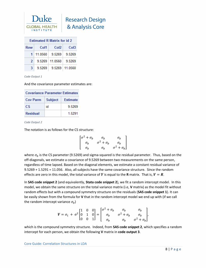
Code Output 1
And the covariance parameter estimates are:
Code Output 2
The notation is as follows for the CS structure:
[
𝜎2 + 𝜎𝑏 𝜎𝑏 𝜎𝑏
𝜎𝑏 𝜎2 + 𝜎𝑏 𝜎𝑏
𝜎𝑏 𝜎𝑏 𝜎2 + 𝜎𝑏
]
where 𝜎𝑏 is the CS parameter (9.5269) and sigma-squared is the residual parameter. Thus, based on the
off-diagonals, we estimate a covariance of 9.5269 between two measurements on the same person,
regardless of time lapsed. Based on the diagonal elements, we estimate a constant residual variance of
9.5269 + 1.5291 = 11.056. Also, all subjects have the same covariance structure. Since the random
effects are zero in this model, the total variance of 𝒀 is equal to the R matrix. That is, 𝑽 = 𝑹.
In SAS code snippet 2 (and equivalently, Stata code snippet 2), we fit a random intercept model. In this
model, we obtain the same structure on the total variance matrix (i.e, V matrix) as the model fit without
random effects but with a compound symmetry structure on the residuals (SAS code snippet 1). It can
be easily shown from the formula for V that in the random intercept model we end up with (if we call
the random intercept variance 𝜎𝑏)
𝑽 = 𝜎1 + σ2 [1 0 00 1 00 0 1
] = [
𝜎2 + 𝜎𝑏 𝜎𝑏 𝜎𝑏
𝜎𝑏 𝜎2 + 𝜎𝑏 𝜎𝑏
𝜎𝑏 𝜎𝑏 𝜎2 + 𝜎𝑏
],
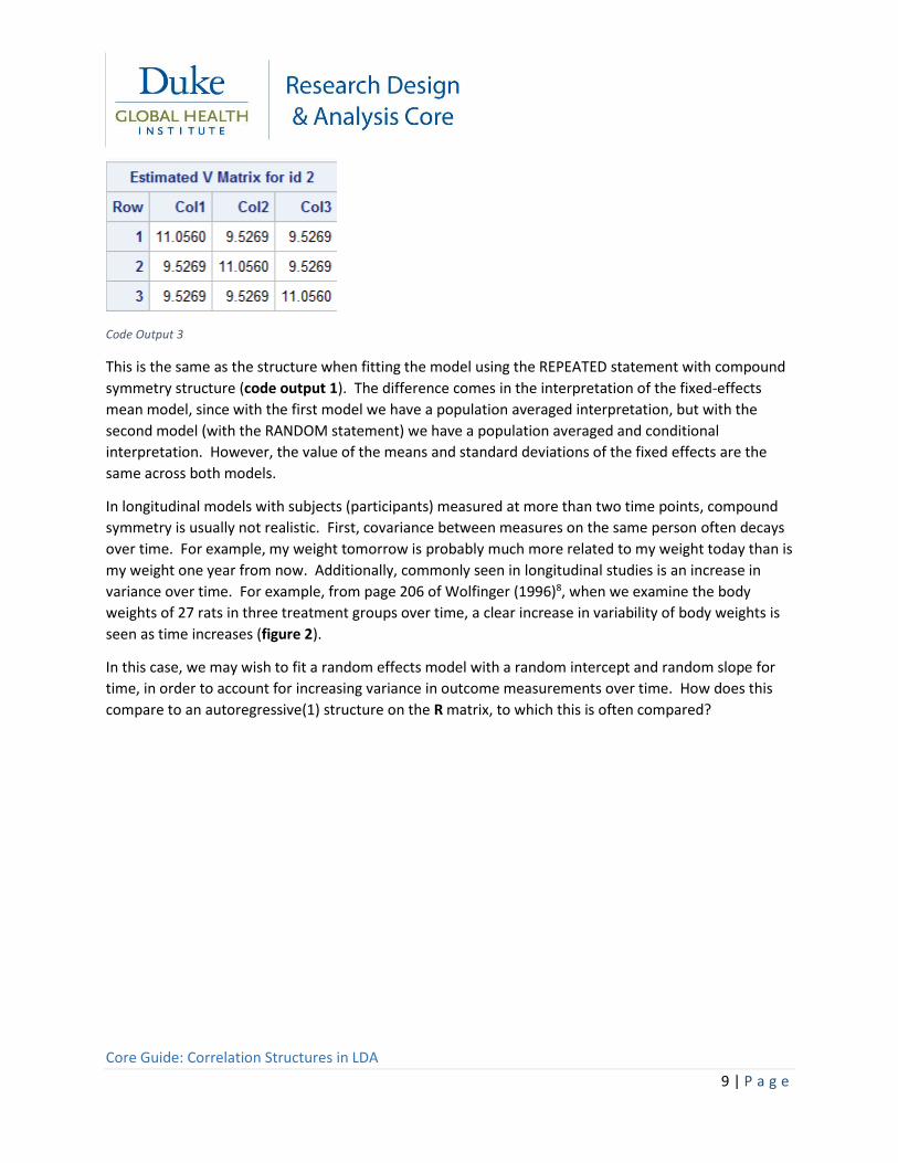
which is the compound symmetry structure. Indeed, from SAS code snippet 2, which specifies a random
intercept for each person, we obtain the following V matrix in code output 3.
Core Guide: Correlation Structures in LDA
9 | P a g e
Code Output 3
This is the same as the structure when fitting the model using the REPEATED statement with compound
symmetry structure (code output 1). The difference comes in the interpretation of the fixed-effects
mean model, since with the first model we have a population averaged interpretation, but with the
second model (with the RANDOM statement) we have a population averaged and conditional
interpretation. However, the value of the means and standard deviations of the fixed effects are the
same across both models.
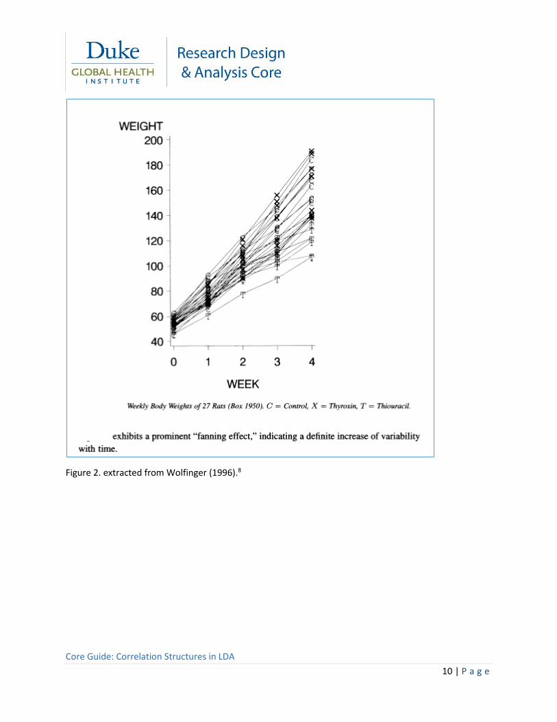
In longitudinal models with subjects (participants) measured at more than two time points, compound
symmetry is usually not realistic. First, covariance between measures on the same person often decays
over time. For example, my weight tomorrow is probably much more related to my weight today than is
my weight one year from now. Additionally, commonly seen in longitudinal studies is an increase in
variance over time. For example, from page 206 of Wolfinger (1996)8, when we examine the body
weights of 27 rats in three treatment groups over time, a clear increase in variability of body weights is
seen as time increases (figure 2).
In this case, we may wish to fit a random effects model with a random intercept and random slope for
time, in order to account for increasing variance in outcome measurements over time. How does this
compare to an autoregressive(1) structure on the R matrix, to which this is often compared?
Core Guide: Correlation Structures in LDA
10 | P a g e
Figure 2. extracted from Wolfinger (1996).8
Core Guide: Correlation Structures in LDA
11 | P a g e
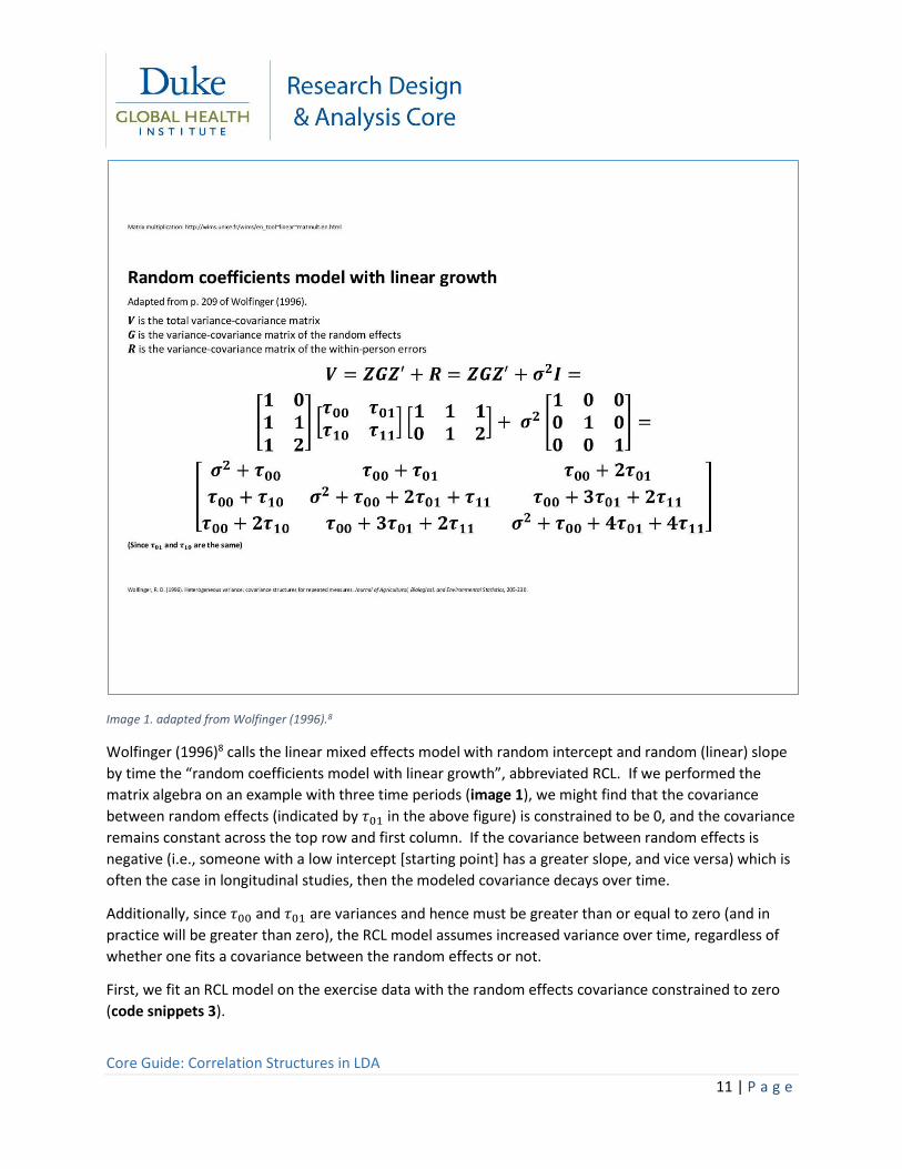
Image 1. adapted from Wolfinger (1996).8
Wolfinger (1996)8 calls the linear mixed effects model with random intercept and random (linear) slope
by time the “random coefficients model with linear growth”, abbreviated RCL. If we performed the
matrix algebra on an example with three time periods (image 1), we might find that the covariance
between random effects (indicated by 𝜏01 in the above figure) is constrained to be 0, and the covariance
remains constant across the top row and first column. If the covariance between random effects is
negative (i.e., someone with a low intercept [starting point] has a greater slope, and vice versa) which is
often the case in longitudinal studies, then the modeled covariance decays over time.
Additionally, since 𝜏00 and 𝜏01 are variances and hence must be greater than or equal to zero (and in
practice will be greater than zero), the RCL model assumes increased variance over time, regardless of
whether one fits a covariance between the random effects or not.
First, we fit an RCL model on the exercise data with the random effects covariance constrained to zero
(code snippets 3).
Core Guide: Correlation Structures in LDA
12 | P a g e
SAS code snippet 3: proc mixed data=long_final;
class id program time;
model strength=program time program*time / s chisq;
random INTERCEPT time_cont / subject=id G GCORR V=1,2 VCORR;
run;
The equivalent Stata code is:
Stata code snippet 3: /* equivalent of SAS random statement with random intercept and slope but no covariance */ mixed strength i.program i.time i.program#i.time, reml || id: time
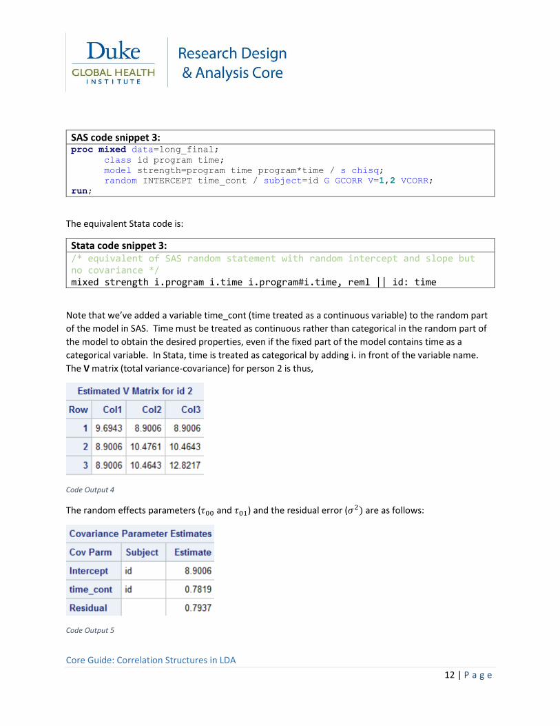
Note that we’ve added a variable time_cont (time treated as a continuous variable) to the random part
of the model in SAS. Time must be treated as continuous rather than categorical in the random part of
the model to obtain the desired properties, even if the fixed part of the model contains time as a
categorical variable. In Stata, time is treated as categorical by adding i. in front of the variable name.
The V matrix (total variance-covariance) for person 2 is thus,
Code Output 4
The random effects parameters (𝜏00 and 𝜏01) and the residual error (𝜎2) are as follows:
Code Output 5
Core Guide: Correlation Structures in LDA
13 | P a g e
If we fit an unstructured covariance matrix to the random effects, allowing for a covariance between
random intercept and slope, we fit the following code (code snippets 4).
SAS code snippet 4: proc mixed data=long_final;
class id program time;
model strength=program time program*time / s chisq;
random INTERCEPT time_cont / type=un subject=id G GCORR V=1,2 VCORR;
run;
The equivalent Stata code is:
Stata code snippet 4: /* equivalent of SAS random statement with random intercept and slope and covariance between the two */ mixed strength i.program i.time i.program#i.time, reml || id: time, covariance(un)
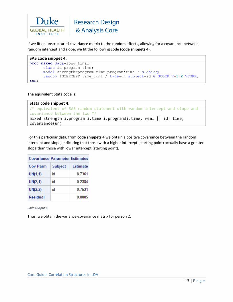
For this particular data, from code snippets 4 we obtain a positive covariance between the random
intercept and slope, indicating that those with a higher intercept (starting point) actually have a greater
slope than those with lower intercept (starting point).
Code Output 6
Thus, we obtain the variance-covariance matrix for person 2:
Core Guide: Correlation Structures in LDA
14 | P a g e
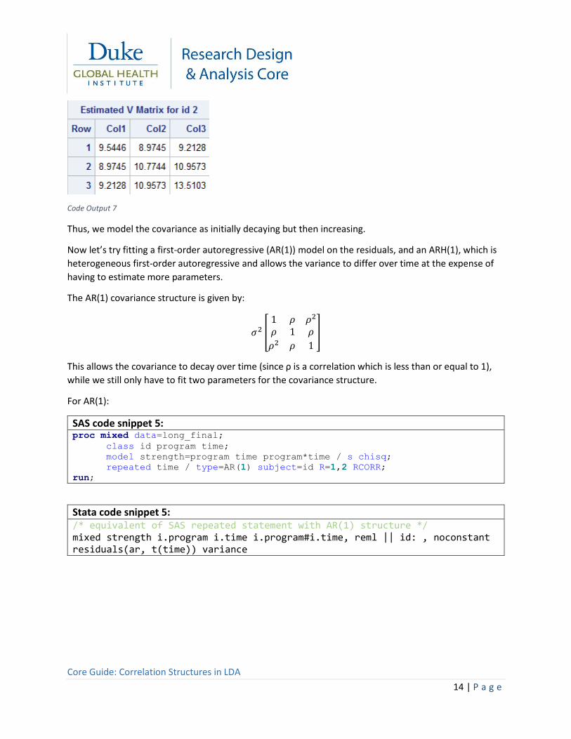
Code Output 7
Thus, we model the covariance as initially decaying but then increasing.
Now let’s try fitting a first-order autoregressive (AR(1)) model on the residuals, and an ARH(1), which is
heterogeneous first-order autoregressive and allows the variance to differ over time at the expense of
having to estimate more parameters.
The AR(1) covariance structure is given by:
𝜎2 [
1 𝜌 𝜌2
𝜌 1 𝜌
𝜌2 𝜌 1
]
This allows the covariance to decay over time (since ρ is a correlation which is less than or equal to 1),
while we still only have to fit two parameters for the covariance structure.
For AR(1):
SAS code snippet 5: proc mixed data=long_final;
class id program time;
model strength=program time program*time / s chisq;
repeated time / type=AR(1) subject=id R=1,2 RCORR;
run;
Stata code snippet 5: /* equivalent of SAS repeated statement with AR(1) structure */ mixed strength i.program i.time i.program#i.time, reml || id: , noconstant residuals(ar, t(time)) variance
Core Guide: Correlation Structures in LDA
15 | P a g e
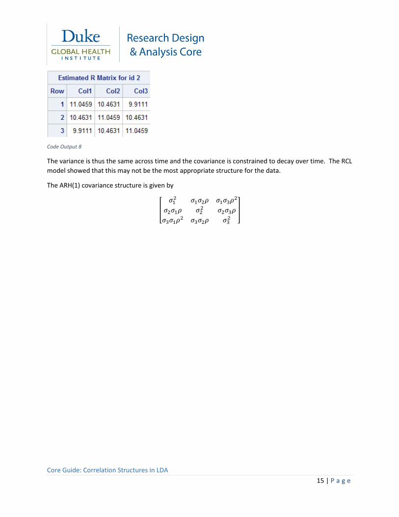
Code Output 8
The variance is thus the same across time and the covariance is constrained to decay over time. The RCL
model showed that this may not be the most appropriate structure for the data.
The ARH(1) covariance structure is given by
[
𝜎12 𝜎1𝜎2𝜌 𝜎1𝜎3𝜌2
𝜎2𝜎1𝜌 𝜎22 𝜎2𝜎3𝜌
𝜎3𝜎1𝜌2 𝜎3𝜎2𝜌 𝜎32
]
Core Guide: Correlation Structures in LDA
16 | P a g e
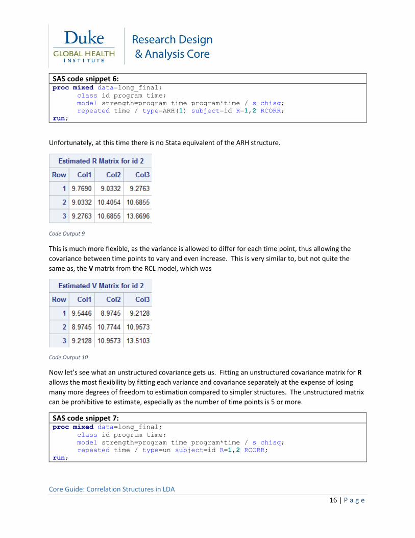
SAS code snippet 6: proc mixed data=long_final;
class id program time;
model strength=program time program*time / s chisq;
repeated time / type=ARH(1) subject=id R=1,2 RCORR;
run;
Unfortunately, at this time there is no Stata equivalent of the ARH structure.
Code Output 9
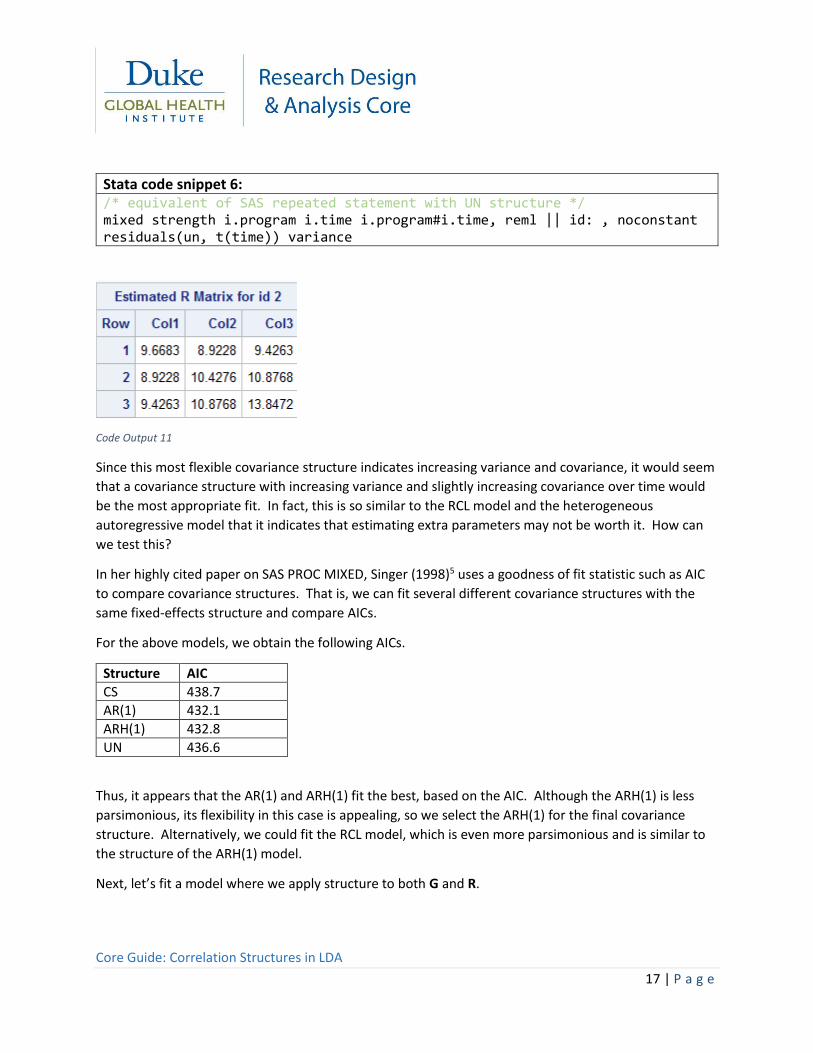
This is much more flexible, as the variance is allowed to differ for each time point, thus allowing the
covariance between time points to vary and even increase. This is very similar to, but not quite the
same as, the V matrix from the RCL model, which was
Code Output 10
Now let’s see what an unstructured covariance gets us. Fitting an unstructured covariance matrix for R
allows the most flexibility by fitting each variance and covariance separately at the expense of losing
many more degrees of freedom to estimation compared to simpler structures. The unstructured matrix
can be prohibitive to estimate, especially as the number of time points is 5 or more.
SAS code snippet 7: proc mixed data=long_final;
class id program time;
model strength=program time program*time / s chisq;
repeated time / type=un subject=id R=1,2 RCORR;
run;
Core Guide: Correlation Structures in LDA
17 | P a g e
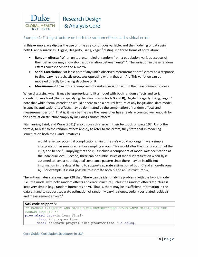
Stata code snippet 6: /* equivalent of SAS repeated statement with UN structure */ mixed strength i.program i.time i.program#i.time, reml || id: , noconstant residuals(un, t(time)) variance
Code Output 11
Since this most flexible covariance structure indicates increasing variance and covariance, it would seem
that a covariance structure with increasing variance and slightly increasing covariance over time would
be the most appropriate fit. In fact, this is so similar to the RCL model and the heterogeneous
autoregressive model that it indicates that estimating extra parameters may not be worth it. How can
we test this?
In her highly cited paper on SAS PROC MIXED, Singer (1998)5 uses a goodness of fit statistic such as AIC
to compare covariance structures. That is, we can fit several different covariance structures with the
same fixed-effects structure and compare AICs.
For the above models, we obtain the following AICs.
Structure AIC
CS 438.7
AR(1) 432.1
ARH(1) 432.8
UN 436.6
Thus, it appears that the AR(1) and ARH(1) fit the best, based on the AIC. Although the ARH(1) is less
parsimonious, its flexibility in this case is appealing, so we select the ARH(1) for the final covariance
structure. Alternatively, we could fit the RCL model, which is even more parsimonious and is similar to
the structure of the ARH(1) model.
Next, let’s fit a model where we apply structure to both G and R.
Core Guide: Correlation Structures in LDA
18 | P a g e
Example 2: Fitting structure on both the random effects and residual error
In this example, we discuss the use of time as a continuous variable, and the modeling of data using
both G and R matrices. Diggle, Heagerty, Liang, Zeger 9 distinguish three forms of correlation:
Random effects: “When units are sampled at random from a population, various aspects of
their behaviour may show stochastic variation between units” 9. The variation in these random
effects corresponds to the G matrix.
Serial Correlation: “At least part of any unit’s observed measurement profile may be a response
to time-varying stochastic processes operating within that unit” 9. This variation can be
modeled directly by placing structure on R.
Measurement Error: This is composed of random variation within the measurement process.
When discussing when it may be appropriate to fit a model with both random effects and serial
correlation modeled (that is, specifying the structure on both G and R), Diggle, Heagerty, Liang, Zeger 9
note that while “serial correlation would appear to be a natural feature of any longitudinal data model,
in specific applications its effects may be dominated by the combination of random effects and
measurement error.” That is, it may be the case the researcher has already accounted well enough for
the correlation structure simply by including random effects.
Fitzmaurice, Laird, and Ware (2011)1 also discuss this issue in their textbook on page 197. Using the
term 𝑏𝑖 to refer to the random effects and 𝜀𝑖𝑗 to refer to the errors, they state that in modeling
structure on both the G and R matrices
would raise two potential complications. First, the 𝜀𝑖𝑗’s would no longer have a simple
interpretation as measurement or sampling errors. This would alter the interpretation of the
𝜀𝑖𝑗’s, and hence 𝑏𝑖, implying that the 𝜀𝑖𝑗’s include a component of model misspecification at
the individual level. Second, there can be subtle issues of model identification when 𝑅𝑖 is
assumed to have a non-diagonal covariance pattern since there may be insufficient
information in the data at hand to support separate estimation of both 𝐺 and a non-diagonal
𝑅𝑖. For example, it is not possible to estimate both 𝐺 and an unstructured 𝑅𝑖.
The authors later state on page 228 that “there can be identifiability problems with the hybrid model
[i.e., the model with both random effects and error structure] unless the random effects structure is
kept very simple (e.g., random intercepts only). That is, there may be insufficient information in the
data at hand to support separate estimation of randomly varying slopes, serially correlated residuals,
and measurement errors”.1
SAS code snippet 8: /* RANDOM INTERCEPT AND SLOPE WITH UNSTRUCTURED COVARIANCE MATRIX FOR THE
RANDOM EFFECTS */
proc mixed data=in.long_final;
class id program time;
model strength=program time program*time / s chisq;
Core Guide: Correlation Structures in LDA
19 | P a g e
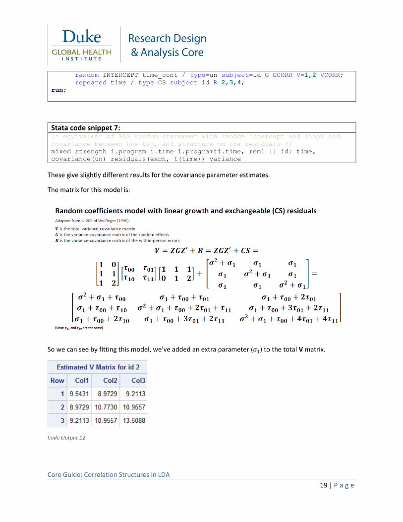
random INTERCEPT time_cont / type=un subject=id G GCORR V=1,2 VCORR;
repeated time / type=CS subject=id R=2,3,4;
run;
Stata code snippet 7: /* equivalent of SAS random statement with random intercept and slope and
covariance between the two, and structure on the residuals */
mixed strength i.program i.time i.program#i.time, reml || id: time,
covariance(un) residuals(exch, t(time)) variance
These give slightly different results for the covariance parameter estimates.
The matrix for this model is:
So we can see by fitting this model, we’ve added an extra parameter (𝜎1) to the total V matrix.
Code Output 12
Core Guide: Correlation Structures in LDA
20 | P a g e
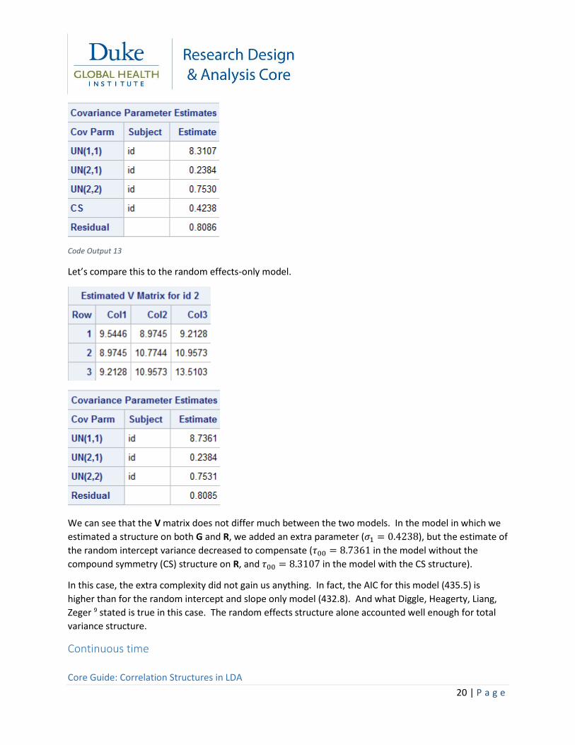
Code Output 13
Let’s compare this to the random effects-only model.
We can see that the V matrix does not differ much between the two models. In the model in which we
estimated a structure on both G and R, we added an extra parameter (𝜎1 = 0.4238), but the estimate of
the random intercept variance decreased to compensate (𝜏00 = 8.7361 in the model without the
compound symmetry (CS) structure on R, and 𝜏00 = 8.3107 in the model with the CS structure).
In this case, the extra complexity did not gain us anything. In fact, the AIC for this model (435.5) is
higher than for the random intercept and slope only model (432.8). And what Diggle, Heagerty, Liang,
Zeger 9 stated is true in this case. The random effects structure alone accounted well enough for total
variance structure.
Continuous time
Core Guide: Correlation Structures in LDA
21 | P a g e
For time which is truly considered continuous, such as data collected from electronic health records
(EHR), some of the structures mentioned above are not appropriate. For example, it doesn’t make
sense to use the autoregressive structure, as we will fit the same covariance between time 1 and 2 (etc.)
for each individual, regardless of whether time 1 and 2 are 1 day apart for one individual or 1 year apart
for another.
In such cases modeling random effects for intercept and slope (and possibly polynomials of slope) offers
the flexibility of modeling an individual-specific intercept and slope while taking into account the within-
subject correlation, regardless of the number of measurements on each individual or the time difference
between measurements.
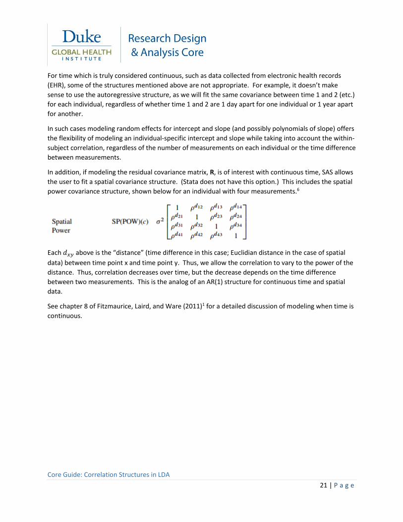
In addition, if modeling the residual covariance matrix, R, is of interest with continuous time, SAS allows
the user to fit a spatial covariance structure. (Stata does not have this option.) This includes the spatial
power covariance structure, shown below for an individual with four measurements.6
Each 𝑑𝑥𝑦 above is the “distance” (time difference in this case; Euclidian distance in the case of spatial
data) between time point x and time point y. Thus, we allow the correlation to vary to the power of the
distance. Thus, correlation decreases over time, but the decrease depends on the time difference
between two measurements. This is the analog of an AR(1) structure for continuous time and spatial
data.
See chapter 8 of Fitzmaurice, Laird, and Ware (2011)1 for a detailed discussion of modeling when time is
continuous.