Copyright Stephen Christopher Johnson

Copyright

by

Stephen Christopher Johnson

1999

Selectively Compliant Orientation Stages for Imprint Lithography

by

Stephen Christopher Johnson, B.S.

Thesis

Presented to the Faculty of the Graduate School

of The University of Texas at Austin

in Partial Fulfillment

of the Requirements

for the Degree of

Master of Science in Engineering

The University of Texas at Austin

May 1999


Approved by

Supervising Committee:

______________________________

______________________________

iv

Acknowledgments

This work would not have been possible without the advice and support of

many people. I would like to thank my advisor, Professor S.V. Sreenivasan for

his guidance and support throughout my graduate career. I would also like to

thank Professor Grant Willson for sharing his extensive knowledge of the

semiconductor industry and teaching by example. I learned a great deal about

spatial kinematics from Jin Choi, and I greatly enjoyed our numerous

conversations over a cup of coffee. Thanks to Matt Colburn for all of his efforts

in developing the first SFIL imprint machine. Thanks to Don Artieschoufsky,

Danny Jarez, and everyone in the mechanical engineering machine shop for

sharing their wisdom and advice. I would also like to thank Ulratech Stepper,

Etec, IBM-Burlington, and Professor Jack Wolfe’s group at the University of

Houston for technical contributions to this work. Thanks to the SRC and DARPA

for financial support. Finally, thanks to all of my colleagues on the Step and

Flash project. I have enjoyed working with you, and my graduate school

experience would not have been the same without you.

May 3, 1999

v


by

Stephen Christopher Johnson, M.S.E.

The University of Texas at Austin, 1999

Supervisor: S. V. Sreenivasan

This document investigates the motion capability of partially constrained

compliant spatial mechanisms. The investigation is directed towards the design of

partially constrained orientation stages for a new imprint lithography process

known as Step and Flash Imprint Lithography. This text begins with an

introduction to this new imprint lithography technology and continues with an

investigation of the compliance matrix eigenvalue problem to compare two

imprint lithography orientation stages. The eigenvalues and eigenvectors of a

compliant structure’s compliance matrix can provide insight into a structure’s

behavior when loaded. The eigenstructure is shown to be effective for examining

the motions of unconstrained or ideal compliant structures. Characterization of

structures that are both partially constrained and non-ideal requires the use of an

alternative metric, that of strain energy imparted to the system. The eigenvalue

problem of these stages is ill-conditioned due to the presence of eigenvalues that

are nearly zero and an eigenvector space that is near-defective. Two orientation

stage designs are shown to have appropriate motion capabilities for imprint

lithography applications. The development of a prototype imprint lithography

machine is described, and experimental results of imprint lithography

demonstrations are included.

vi

Table of Contents

LIST OF FIGURES............................................................................................................. VIII

1 INTRODUCTION............................................................................................................1

1.1 OPTICAL LITHOGRAPHY..................................................................................................1

1.1.1 Process Description..............................................................................................2

1.1.2 Technical Challenges............................................................................................3

1.2 IMPRINT LITHOGRAPHY ..................................................................................................4

1.2.1 Imprint Lithography Process Description..............................................................5

1.2.2 Technical Challenges............................................................................................6

1.3 STEP AND FLASH IMPRINT LITHOGRAPHY ........................................................................7

1.3.1 Template Generation ............................................................................................7

1.3.2 Step and Flash Lithography Process Description ..................................................8

1.3.3 Technical Challenges..........................................................................................10

2 IMPRINT MACHINE DESIGN ....................................................................................12

3 ORIENTATION STAGE DEVELOPMENT.................................................................15

3.1 INTRODUCTION TO SCREW SYSTEM THEORY..................................................................16

3.1.1 Screw axis ($) .....................................................................................................17

3.1.2 Motor ( $v ) ..........................................................................................................19

3.1.3 Wrench ( $f ) ........................................................................................................19

3.1.4 Reciprocity .........................................................................................................19

3.2 FIRST GENERATION ORIENTATION STAGE......................................................................21

3.2.1 Mobility Analysis ................................................................................................21

3.2.2 Detailed Design..................................................................................................23

3.3 THE USE OF FLEXURES IN MECHANISM DESIGN .............................................................25

3.4 SECOND GENERATION LUMPED FLEXURE STAGE ...........................................................27

3.4.1 Mobility Analysis ................................................................................................27

3.4.2 Detailed Design..................................................................................................29

3.5 THIRD GENERATION DISTRIBUTED FLEXURE STAGE ......................................................29

4 MOBILITY ANALYSIS ................................................................................................33

viii

vii

4.1 BASIS OF COMPARISON .................................................................................................33

4.1.1 Wrenches, Twists, and the Compliance Matrix ....................................................33

4.2 IDEAL KINEMATIC STAGE .............................................................................................36

4.2.1 Compliance Matrix .............................................................................................36

4.2.2 Eigenscrews and Eigenvalues .............................................................................40

4.3 DISTRIBUTED FLEXURE STAGE......................................................................................42

4.3.1 Finite Element Model..........................................................................................42

4.3.2 Analysis of Wrench and Twist Matrices...............................................................46

4.3.3 Eigenvalues and Eigenvectors.............................................................................48

4.3.4 The Use of Strain Energy as a Metric..................................................................54

4.4 SUMMARY....................................................................................................................56

5 EXPERIMENTAL RESULTS .......................................................................................57

5.1 IMAGES ON FLAT SUBSTRATES......................................................................................57

5.2 IMAGES ON CURVED SUBSTRATES .................................................................................59

6 CLOSING REMARKS...................................................................................................61

6.1 CONCLUSIONS ..............................................................................................................61

6.2 FUTURE WORK .............................................................................................................62

6.2.1 Base Layer Thickness..........................................................................................62

6.2.2 Scientific Investigation........................................................................................64

6.2.3 Sensing...............................................................................................................64

6.2.4 Active and Passive Stages ...................................................................................65

6.2.5 Overlay ..............................................................................................................66

6.2.6 Template Loading and Deformation....................................................................66

APPENDIX A ..........................................................................................................................67

APPENDIX B ..........................................................................................................................69

REFERENCES........................................................................................................................78

VITA........................................................................................................................................80

viii

List of Figures

FIGURE 1.1 OPTICAL LITHOGRAPHY PROCESS ...............................................................................2

FIGURE 1.2 IMPRINT LITHOGRAPHY PROCESS ...............................................................................5

FIGURE 1.3 IMPRINT LITHOGRAPHY PATTERN DENSITY DEPENDENCE .............................................7

FIGURE 1.4 STEP AND FLASH IMPRINT LITHOGRAPHY PROCESS ......................................................9

FIGURE 2.1 STEP AND FLASH PRESS ............................................................................................13

FIGURE 3.1 ANGULAR MISALIGNMENT BETWEEN TEMPLATE AND MASK .......................................15

FIGURE 3.2 DESIRED AND UNDESIRED MOTIONS BETWEEN TEMPLATE AND WAFER .......................16

FIGURE 3.3 THE GEOMETRY OF THE VELOCITY FIELD OF POINTS IN A RIGID BODY .........................18

FIGURE 3.4 A RECIPROCAL WRENCH, $f , APPLIED TO A BODY WITH 5TH ORDER MOTION SCREW ....20

FIGURE 3.5 IDEAL ORIENTATION STAGE KINEMATIC MODEL.........................................................21

FIGURE 3.6 WRENCHES RECIPROCAL TO ORIENTATION STAGE .....................................................22

FIGURE 3.7 INITIAL WAFER ORIENTATION STAGE ........................................................................24

FIGURE 3.8 REVOLUTE JOINT AND CORRESPONDING FLEXURE .....................................................25

FIGURE 3.9 LUMPED FLEXURE STAGE ........................................................................................27

FIGURE 3.10 WRENCHES RECIPROCAL TO LUMPED FLEXURE STAGE .............................................28

FIGURE 3.11 DISTRIBUTED FLEXURE ORIENTATION STAGE ..........................................................30

FIGURE 3.12 FIXED-FIXED BEAM ................................................................................................31

FIGURE 4.1 SCREW REPRESENTATION OF THREE LEG MODEL .......................................................37

FIGURE 4.2 FINITE ELEMENT MODEL...........................................................................................44

FIGURE 4.3 DEFLECTED FINITE ELEMENT MODEL ........................................................................45

FIGURE 4.4 FLEXURE STAGE COORDINATE FRAME.......................................................................47

FIGURE 5.1 AFM IMAGE OF 20 µM FEATURE ..............................................................................57

FIGURE 5.2 AFM IMAGE OF SUB-MICRON LINES AND SPACES.......................................................58

FIGURE 5.3 60 NM FEATURES ON TEMPLATE* AND ETCH BARRIER................................................58

FIGURE 5.4 150 NM FEATURES IN ETCH BARRIER .........................................................................59

FIGURE 5.5 OPTICAL MICROGRAPHS OF IMAGES ON CURVED TEMPLATE AND SUBSTRATE..............60

FIGURE 5.6 SEM AND AFM IMAGES OF PATTERNED SPHERICAL SUBSTRATE................................60

FIGURE 6.1 RESIDUAL BASE LAYER ............................................................................................62

1

1 Introduction

The parallel transfer of high-resolution patterns over large areas has

become a focal point of research in the semiconductor industry. The process of

transferring sub-micron features onto wafers, referred to as lithography, is one of

the key technologies in manufacturing semiconductor devices. Circuits with

small components operate at high speeds. Smaller circuits also allow

semiconductor manufacturers to increase profits by placing more circuits on one

wafer. These economic forces have driven the microelectronics industry to invest

hundred of millions of dollars in researching next generation lithography

techniques.

Optical lithography currently satisfies manufacturers’ requirements and is

the process of choice for semiconductor companies. 0.2 micron devices are

currently manufactured with optical lithography. However, may believe that

optical limits hinder the cost-effective generation of circuits with still smaller

components. The Semiconductor Industry Association Roadmap outlines cost

and timetables for developing alternative lithography techniques capable of

imaging features smaller than 100 nm. This chapter describes the optical

lithography process, examines some of the limitations of optical lithography, and

presents two alternative high-resolution pattern transfer technologies.

1.1 Optical Lithography

The semiconductor industry currently uses optical lithography to produce

integrated circuits. This well established process generates patterns on silicon

wafers using an optical projection technique. A layer of photosensitive polymer

absorbs an aerial image that is then chemically transferred to the wafer.

2

1.1.1 Process Description

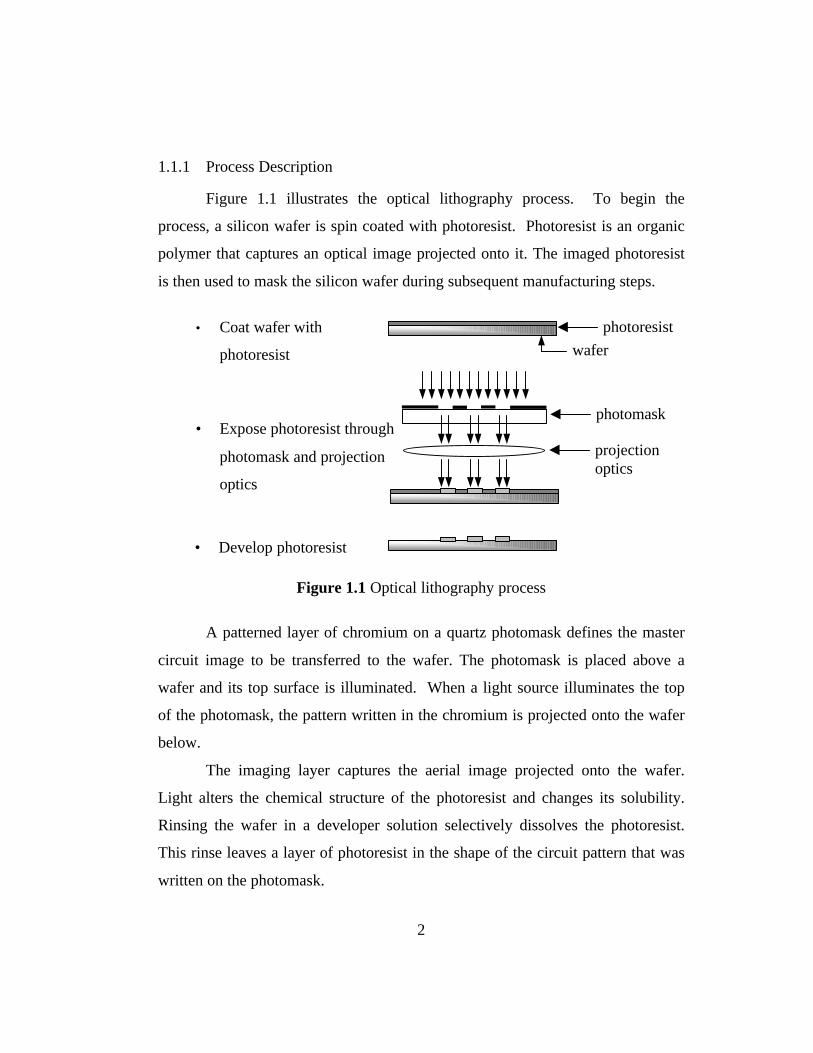
Figure 1.1 illustrates the optical lithography process. To begin the

process, a silicon wafer is spin coated with photoresist. Photoresist is an organic

polymer that captures an optical image projected onto it. The imaged photoresist

is then used to mask the silicon wafer during subsequent manufacturing steps.

Figure 1.1 Optical lithography process

A patterned layer of chromium on a quartz photomask defines the master

circuit image to be transferred to the wafer. The photomask is placed above a

wafer and its top surface is illuminated. When a light source illuminates the top

of the photomask, the pattern written in the chromium is projected onto the wafer

below.

The imaging layer captures the aerial image projected onto the wafer.

Light alters the chemical structure of the photoresist and changes its solubility.

Rinsing the wafer in a developer solution selectively dissolves the photoresist.

This rinse leaves a layer of photoresist in the shape of the circuit pattern that was

written on the photomask.

• Coat wafer with

photoresist

• Expose photoresist through

photomask and projection

optics

• Develop photoresist

wafer

photoresist

photomask

projectionoptics

3

Once the photomask has been patterned, it serves as an etch or ion

implantation mask. A chemical etch removes areas of underlying substrate not

protected by the patterned photoresist. The remaining photoresist is then stripped

from the wafer. The end result of this process is a pattern transfer into the

substrate. These patterns in resist are used to control the patterning and placement

of various steps required to manufacture a microelectronic circuit.

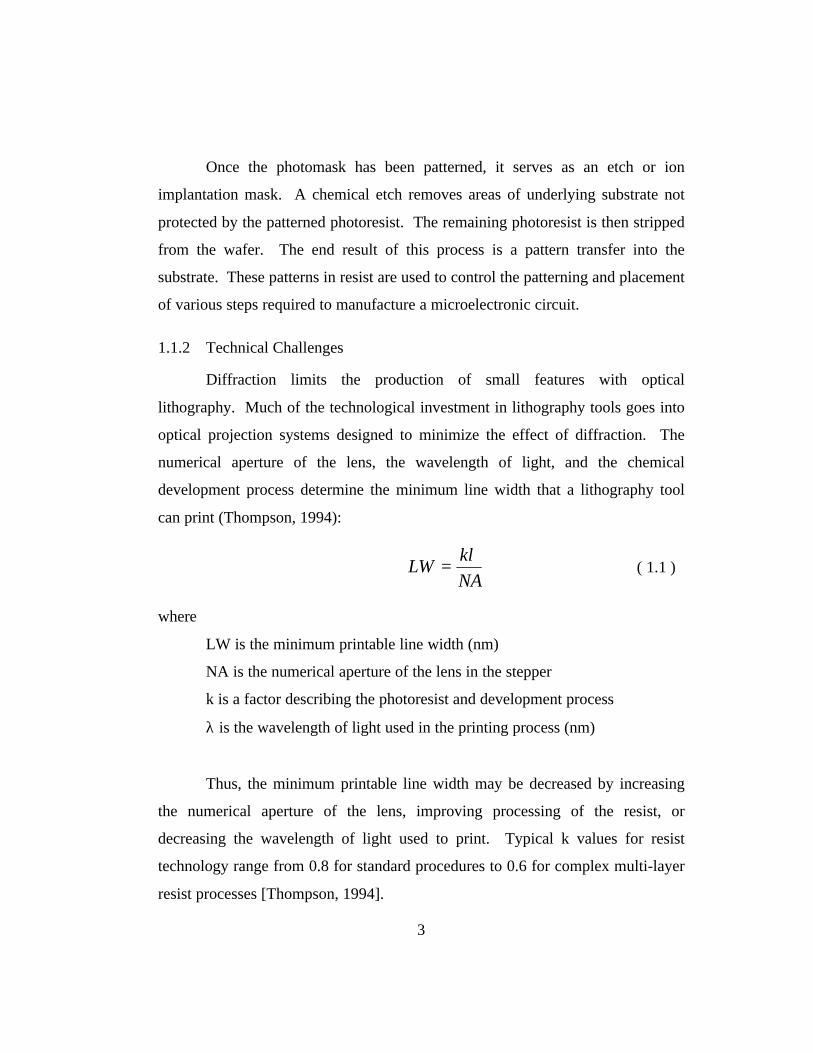
1.1.2 Technical Challenges

Diffraction limits the production of small features with optical

lithography. Much of the technological investment in lithography tools goes into

optical projection systems designed to minimize the effect of diffraction. The

numerical aperture of the lens, the wavelength of light, and the chemical

development process determine the minimum line width that a lithography tool

can print (Thompson, 1994):

NA

kLW

λ= ( 1.1 )

where

LW is the minimum printable line width (nm)

NA is the numerical aperture of the lens in the stepper

k is a factor describing the photoresist and development process

λ is the wavelength of light used in the printing process (nm)

Thus, the minimum printable line width may be decreased by increasing

the numerical aperture of the lens, improving processing of the resist, or

decreasing the wavelength of light used to print. Typical k values for resist

technology range from 0.8 for standard procedures to 0.6 for complex multi-layer

resist processes [Thompson, 1994].

4

The numerical aperture of a lens is a measure of what angle light may

enter the lens. Increasing the numerical aperture of a lens while maintaining

allowable field sizes, requires must increasing the size of the lens. Large lenses

are more difficult to manufacture and, thus, more expensive. It is not uncommon

for lens systems in today’s step and repeat photolithography tools to weigh

hundreds of pounds and cost several million dollars.

Investments in reducing the wavelength of light used to print images have

reduced minimum printable line widths. Many of today’s steppers use 248 nm

deep ultraviolet (DUV) light to image wafers. 193 nm and 157 nm systems are in

development and will further decrease minimum printable line widths. 15 nm

extreme ultraviolet (EUV) and x-ray lithography technologies offer potential for

decreasing line widths to even smaller dimensions, but these techniques present

significant technical challenges and prohibitive cost. Materials that are

transparent to DUV light are opaque in the EUV and x-ray regions, so these new

technologies will have to develop expensive new optics technologies.

Furthermore, EUV and x-ray sources with sufficient intensity to print images are

rare and expensive. The technical challenge and cost of implementing EUV and

x-ray lithography technologies clearly warrant the investigation of other pattern

transfer technologies for use in the semiconductor and micro-machining

industries.

1.2 Imprint Lithography

Imprint lithography offers an alternative high-resolution pattern transfer

technology. In this process, a template is pressed into a thermoplastic. The

polymer conforms to a relief image of a circuit in the template. As this approach

uses no optics, diffraction does not limit minimum printable line widths. The

topography of the imprint template defines the pattern transferred to the silicon

5

wafer. A typical imprint lithography is described next. Professor Chou, et. al., at

Princeton have studied various versions of this process for micro-machining and

lithography applications.

1.2.1 Imprint Lithography Process Description

Figure 1.2 illustrates a typical imprint lithography process. To begin the

process, a wafer is spin-coated with a thermoplastic and a transfer layer. The

thermoplastic is heated to its glass transition temperature so that it can flow, and a

template is then pressed into the pliable thermoplastic. Once the thermoplastic

has conformed to the shape of the template, the assembly is cooled, and the wafer

and template are separated. The image in the thermoplastic is then copied into the

transfer layer and the wafer via chemical etch processes.

Figure 1.2 Imprint lithography process

thermoplastic

wafer

transfer layer

template

• Heat polymer above Tg

• Press mold into template

and cool• Separate template and wafer

• Coat template with

thermoplastic and

transfer layer

• Etch through transfer layer

• Strip thermoplastic

6


Imprint lithography faces two distinct challenges: overlay and image

transfer fidelity. High temperatures and pressures during the image transfer

process distort the template and wafer. Quartz and polysilicon have coefficients

of thermal expansion of 4.8e-7 °C-1 and 4.2e-6 °C-1 respectively. A temperate

change of 300 °C would cause a 25 mm quartz template to elongate 3.66 microns.

A 75 mm diameter silicon wafer would suffer a 96 micron change in dimension.

Pressures on the order of hundreds of psi would cause similarly large distortions

in the wafer and template. Such changes in dimension are clearly unacceptable

when printing sub-100 nm features.

Such dimensional instabilities make it extremely difficult if not impossible

to overlay multiple layers of an integrated circuit. An overlay scheme for such a

system would have to account for thermal and mechanical distortions in the

template and wafer. It is important to note that these distortions will depend on

the process parameters (i.e. temperate and pressure) of every step of the image

transfer process. The overlay process will have to be altered every time a process

parameter is altered. While technology and engineering ingenuity may overcome

these obstacles, they will increase the complexity and cost of imprint lithography

and decrease its throughput.

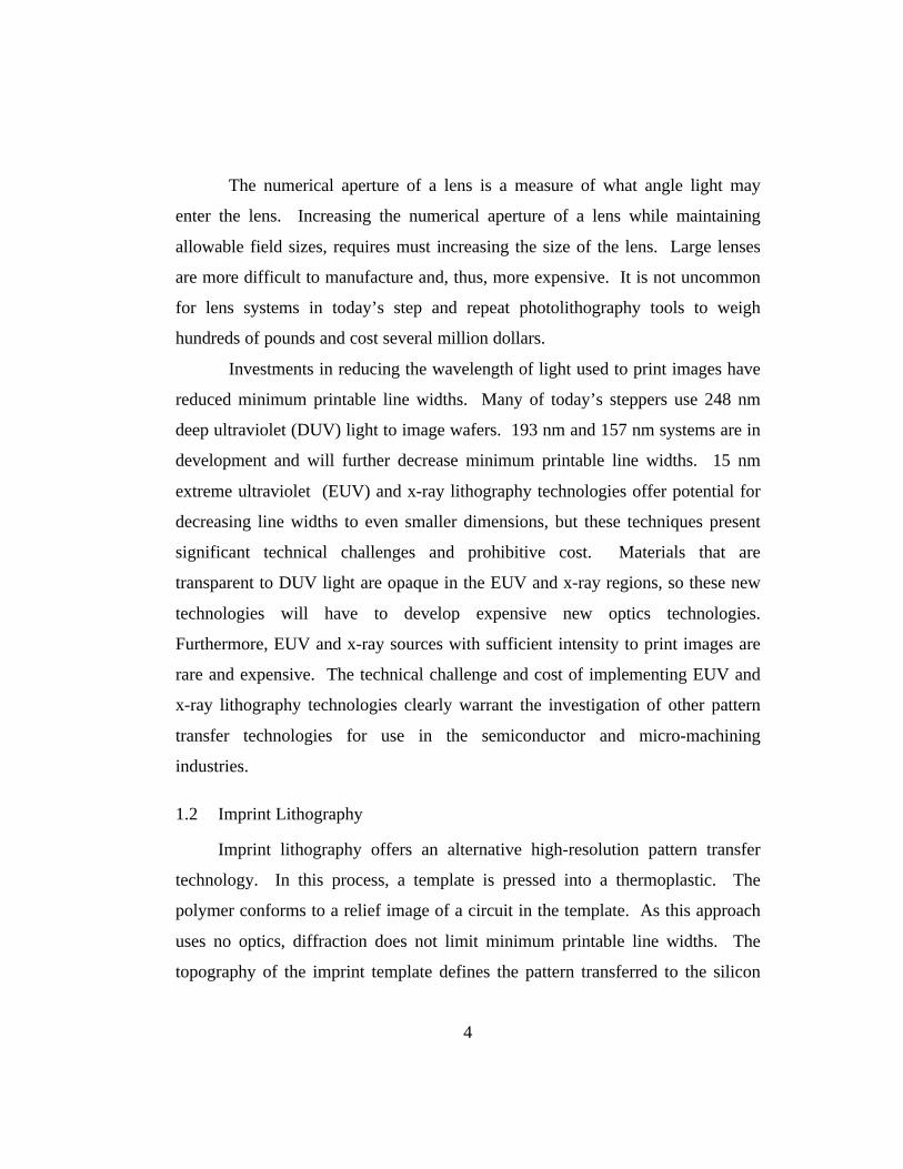
The fidelity of images created with imprint lithography also suffers a

pattern density dependence. As a template is pressed into the heated

thermoplastic, it must displace significant amounts of material. Figure 1.3

illustrates three patterns to be transferred via imprint lithography. Isolated

features that displace little material present little challenge to the imprint

lithography process. Gratings and features that displace moderate amounts of

thermoplastic present significant challenges to the imprint process. Isolated

trenches present an extreme challenge to this process. Any material that does not

7

fill the trench must be displaced to the side of the template. Image fidelity suffers

when patterns incorporate numerous isolated trenches.

Figure 1.3 Imprint lithography pattern density dependence

(from left to right) a) isolated line b) grating structure c) isolated trench.

This pattern density dependence is especially apparent when printing

isolated trenches or large features. These shortcomings have lead researchers at

The University of Texas at Austin to pursue an alternative lithography scheme

known as Step and Flash Imprint Lithography.

1.3 Step and Flash Imprint Lithography

Step and Flash Imprint Lithography (SFIL) offers another means to transfer

images with high resolution, high fidelity, and high throughput. SFIL uses

chemical and mechanical processes to transfer images at room temperature with

minimal force. The topography of a master template defines the pattern

transferred to the wafer, and no projection optics are used.

1.3.1 Template Generation

SFIL is a pattern transfer process and requires a master template. Initial

templates have been fabricated via a process very similar to the one used to

manufacture phase shift masks. A quartz photomask blank is coated with

chromium and a photoresist. The photoresist is patterned with a direct write

electron beam machine, and the pattern is transferred to the chromium. At this

point, the template is essentially a traditional photomask used in optical

lithography. Next, the chromium is used as an etch barrier and the circuit pattern

8

is etched into the quartz. The chromium is then stripped off the quartz. The end

product of this process is a quartz template bearing a relief image of the circuit

pattern.

1.3.2 Step and Flash Lithography Process Description

SFIL could probably best be described as a micro-molding process. A

master template bearing a relief image defines the pattern to be transferred. SFIL

and traditional imprint lithography are similar in the fact that they both use the

topography of a template to define the pattern created on the substrate. No

projection optics are involved. The key difference between SFIL and traditional

imprint lithography is the use of a liquid etch barrier to create a low aspect ratio

pattern much like the 2P process developed at Phillips [Haisma, 1996]. This low

viscosity solution eliminates traditional imprint lithography’s need of high

temperatures and pressures. Once low aspect ratio features have been created in

the etch barrier, they are copied to a transfer layer using a chemical etch process.

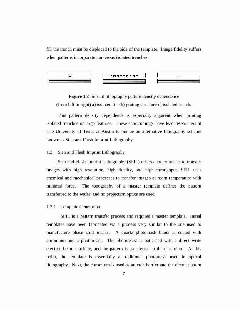
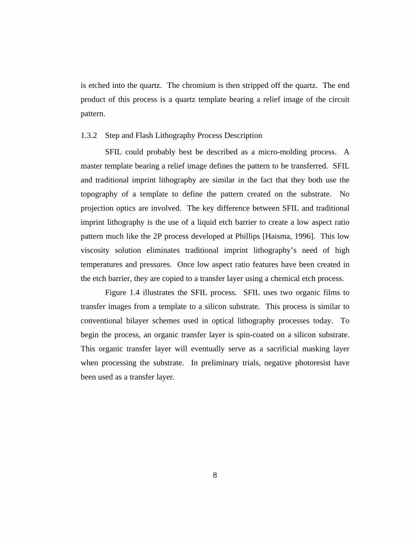
Figure 1.4 illustrates the SFIL process. SFIL uses two organic films to

transfer images from a template to a silicon substrate. This process is similar to

conventional bilayer schemes used in optical lithography processes today. To

begin the process, an organic transfer layer is spin-coated on a silicon substrate.

This organic transfer layer will eventually serve as a sacrificial masking layer

when processing the substrate. In preliminary trials, negative photoresist have

been used as a transfer layer.

9

Figure 1.4 Step and flash imprint lithography process

In the next step of the process, a quartz template bearing the relief image of

a circuit is brought into the proximity of the coated silicon substrate. Once the

substrate and template have been brought into proximity, a drop of a low viscosity

photopolymerizable, organosilicon etch barrier is dispensed. The liquid then fills

the gap between the template and wafer via capillary action [Colburn, 1999]. The

use of a liquid etch barrier gives SFIL its main advantage over traditional imprint

lithography. By shaping a liquid instead of a highly viscous thermoplastic, SFIL

trades the process control parameters of temperature and pressure for material

properties. Developing a SFIL process requires optimization of the chemistry of

the etch barrier, transfer layer, and template surface treatment much more than

temperature and pressure. The lack of varying temperatures and pressures makes

• Oxygen etch throughtransfer layer

• Place template near wafer

• Dispense liquid etch barrier

• Bring template and wafer into

contact and expose with UV

• Remove template

• Coat wafer with transfer layer

• Strip etch barrier

template

etchbarrier

transfer layer

wafer

10

SFIL much more compatible with mechanical alignment and orientation schemes

than traditional imprint lithography.

Once the liquid etch barrier fills the gap via capillary action the template

and wafer are pressed together. The etch barrier is then irradiated with ultraviolet

light through the top side of the template. A blanket ultraviolet exposure cures

the photopolymer and creates a solidified, silicon rich, low surface energy film in

the shape of the circuit image on the template. It is important to note that the

ultraviolet light does not pattern the etch barrier; it simply initiates crosslinking in

the polymer. SFIL uses no projection optics. The patterned template defines the

image transferred to the etch barrier.

Once the photocuring is complete, the template is separated from the

substrate leaving a patterned, cross-linked, silicon containing etch barrier. After

the template and substrate are separated, the pattern in the etch barrier is etched

into the transfer layer. At this point in the process, the silicon substrate is coated

with a sacrificial imaging layer analogous to the imaged substrate created after the

first etch of an optical lithography bilayer process. An oxygen reactive ion etch

may then be used to transfer a high aspect ratio image to the silicon wafer.


Researchers developing SFIL face a number of chemical and mechanical

challenges. Materials research concentrates on the development of appropriate

etch barrier, transfer layer, and template treatment chemistries. The surface

energies of the transfer layer, etch barrier, and template are tuned to draw the

liquid etch barrier into the gap between the template and substrate. To insure

image fidelity, the etch barrier must wet all of the surfaces of the template.

Bubbles or voids in the etch barrier will generate defects in later steps of the

pattern transfer process.

11

In addition to wetting the template, the etch barrier must also release from

the template once it cures. Surface energies of the etch barrier, template, and

transfer layer are tuned such that the cured etch barrier adheres to the transfer

layer and not to the template. A significant portion of the work on this project has

focused on developing materials with surface energies and surface tensions that

meet these requirements. Other research focuses on improving the rate of

polymerization of the etch barrier and identifying etch processes to transfer

patterns from layer to layer.

Another aspect of the research program deals with the design of a machine

to implement Step and Flash Imprint Lithography. Such a machine must hold a

template and a silicon wafer. It must bring them into contact, dispense an etch

barrier solution, and irradiate this structure with ultraviolet light. A focal point of

the machine development deals with the interaction of the template and wafer.

The template and wafer must be in parallel contact when irradiated with

ultraviolet light.

The remainder of this document focuses on the design of a prototype

lithographic press used for initial development studies of SFIL. A passive

selectively compliant stage is developed to obtain large-area contact between a

wafer and a template. This machine allows researchers to investigate the

resolution capability of the SFIL process and develop etch barrier and transfer

layer materials. Future studies will investigate active stages and nanometer

resolution optical sensing schemes to further investigate the template-wafer

interface.

12

2 Imprint Machine Design

A significant portion of SFIL development work has focused on the design

and construction of a lithographic press to implement the SFIL process. Initial

resolution and SFIL process studies required a machine to transfer an image from

a one square inch template to the center of a three inch diameter silicon wafer.

This machine enabled testing of various etch barriers, transfer layers, and

template surface treatments. This machine was also used for many of the first

SFIL image transfer trials.

Such a machine must perform many functions. It must hold the wafer and

template with minimal distortion and damage. It must also bring the wafer and

template into parallel contact. Such a machine must illuminate the template and

wafer with UV light and measure the force required to separate the template and

wafer after curing. Since the machine is used in a research environment, it must

be reasonably simple to modify, and it must allow the user access to the template

and wafer during processing.

Figure 2.1 shows a side view of the SFIL press prototype. To transfer an

image, one first mounts a template in the template seat and places a silicon wafer

on the orientation stage. The template seat and orientation stage lie inside a press

constructed of two horizontal plates and four 24 mm diameter linear roller

bearings constructed by Agathon, Inc. The roller bearings are preloaded to only

allow vertical motion between the template and the wafer. This vertical motion

protects transferred features by minimizing lateral motions between the template

and wafer.

13

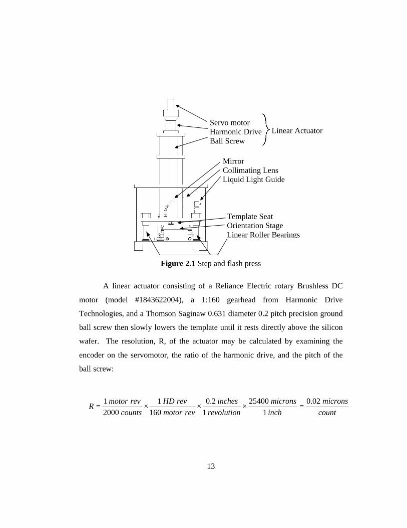
Figure 2.1 Step and flash press

A linear actuator consisting of a Reliance Electric rotary Brushless DC

motor (model #1843622004), a 1:160 gearhead from Harmonic Drive

Technologies, and a Thomson Saginaw 0.631 diameter 0.2 pitch precision ground

ball screw then slowly lowers the template until it rests directly above the silicon

wafer. The resolution, R, of the actuator may be calculated by examining the

encoder on the servomotor, the ratio of the harmonic drive, and the pitch of the

ball screw:

Servo motorHarmonic DriveBall Screw

Linear Actuator

Template SeatOrientation StageLinear Roller Bearings

MirrorCollimating LensLiquid Light Guide

count

microns

inch

microns

revolution

inches

revmotor

revHD

counts

revmotorR

02.0

1

25400

1

2.0

160

1

2000

1=×××=

14

The use of a preloaded ball screw nut and harmonic drive minimize

backlash. Other factors such as compliance of the harmonic drive, motor

feedback errors, ball screw machining errors and thermal drift reduce the accuracy

of the system to the order of tens of microns. The length of the ball screw allows

the template seat to travel almost six inches from its lowest position to its highest

position. This allows for easy installation of any future orientation stage designs

and lets researchers raise the template to inspect or modify a template or wafer

during a printing process.

Once the template rests directly above the wafer, an ultraviolet curable

etch barrier is dispensed and fills the gap between the template and the wafer via

capillary action. After the etch barrier fills the gap between the template and

wafer, the linear actuator presses the template onto the wafer. The wafer is

mounted on a compliant orientation stage that flexes to allow the wafer to match

the orientation of the template. Chapter 3 discusses the orientation stage in

greater detail.

A tripod arrangement of three force sensors below the orientation stage

senses when the template and wafer make contact. After the template and wafer

are pressed together, ultraviolet light illuminates the etch barrier. An Oriel

mercury vapor lamp provides UV light with a peak near 365 nm. A liquid light

guide directs the light into the machine. A lens collimates the light exiting the

liquid guide and a mirror reflects the light onto the template-wafer interface.

After the etch barrier is cross-linked, the linear actuator separates the template and

wafer. The template and wafer may then be removed from the machine for

inspection and further processing.

15

3 Orientation Stage Development

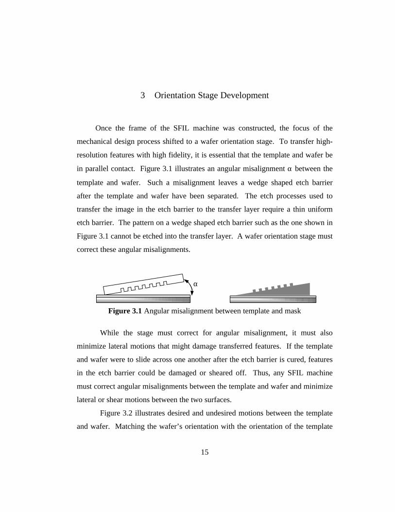
Once the frame of the SFIL machine was constructed, the focus of the

mechanical design process shifted to a wafer orientation stage. To transfer high-

resolution features with high fidelity, it is essential that the template and wafer be

in parallel contact. Figure 3.1 illustrates an angular misalignment α between the

template and wafer. Such a misalignment leaves a wedge shaped etch barrier

after the template and wafer have been separated. The etch processes used to

transfer the image in the etch barrier to the transfer layer require a thin uniform

etch barrier. The pattern on a wedge shaped etch barrier such as the one shown in

Figure 3.1 cannot be etched into the transfer layer. A wafer orientation stage must

correct these angular misalignments.

Figure 3.1 Angular misalignment between template and mask

While the stage must correct for angular misalignment, it must also

minimize lateral motions that might damage transferred features. If the template

and wafer were to slide across one another after the etch barrier is cured, features

in the etch barrier could be damaged or sheared off. Thus, any SFIL machine

must correct angular misalignments between the template and wafer and minimize

lateral or shear motions between the two surfaces.

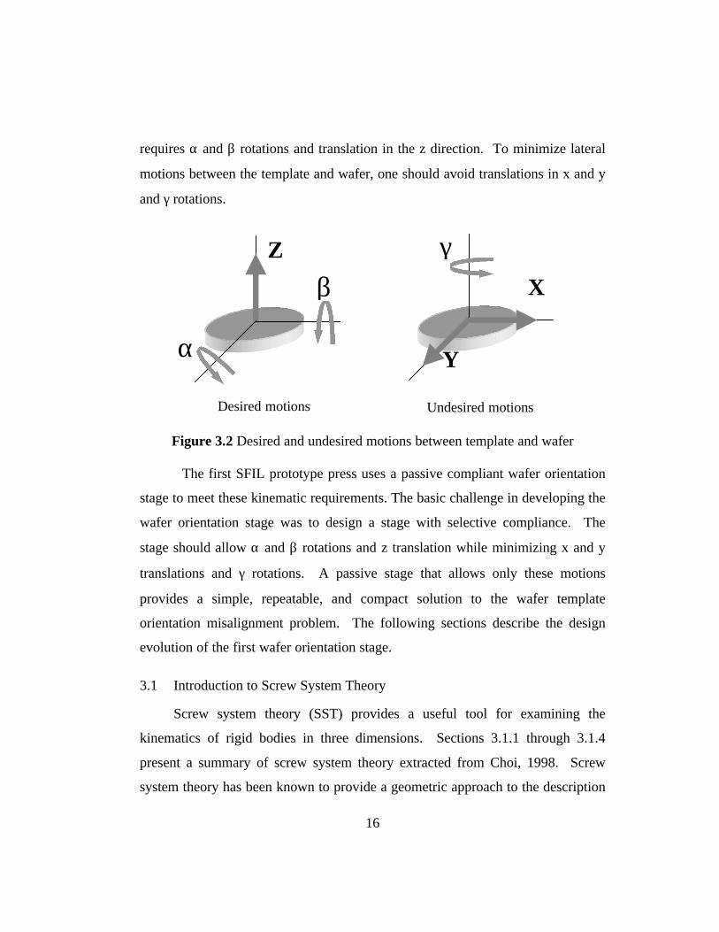
Figure 3.2 illustrates desired and undesired motions between the template

and wafer. Matching the wafer’s orientation with the orientation of the template

α

16

requires α and β rotations and translation in the z direction. To minimize lateral

motions between the template and wafer, one should avoid translations in x and y

and γ rotations.

Figure 3.2 Desired and undesired motions between template and wafer

The first SFIL prototype press uses a passive compliant wafer orientation

stage to meet these kinematic requirements. The basic challenge in developing the

wafer orientation stage was to design a stage with selective compliance. The

stage should allow α and β rotations and z translation while minimizing x and y

translations and γ rotations. A passive stage that allows only these motions

provides a simple, repeatable, and compact solution to the wafer template

orientation misalignment problem. The following sections describe the design

evolution of the first wafer orientation stage.

3.1 Introduction to Screw System Theory

Screw system theory (SST) provides a useful tool for examining the

kinematics of rigid bodies in three dimensions. Sections 3.1.1 through 3.1.4

present a summary of screw system theory extracted from Choi, 1998. Screw

system theory has been known to provide a geometric approach to the description

Z

β

α

X

γ

Y

Desired motions Undesired motions

17

of velocity and force systems associated with systems of rigid bodies. Therefore

SST provides geometric insights which may be obscured by the complex nature of

the analytical models of spatial mechanisms and robotic systems.

3.1.1 Screw axis ($)

A screw is a pure geometric concept which is comprised of a line in space

(screw axis) along with pitch. A screw can be used to denote both spatial velocity

and force systems associated with a rigid body. The concept of a screw is now

developed using the velocity state of a rigid body. The instantaneous motion of a

rigid body moving freely in space can be fully described by six velocity

components: three rotation and three translation velocities. A screw axis is

defined such that all points in the body (or extension of the body) that lie on the

instantaneous screw axis have the same velocity along the screw axis. Such a

screw axis always exists for spatial motion except in the case of pure translation.

This axis is also unique if it exists

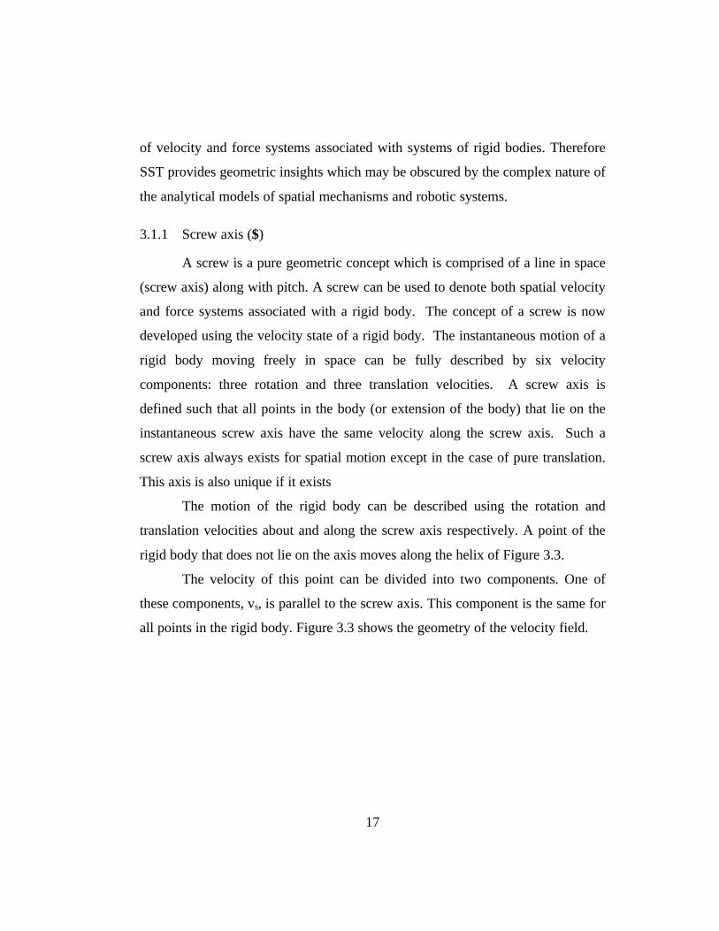
The motion of the rigid body can be described using the rotation and

translation velocities about and along the screw axis respectively. A point of the

rigid body that does not lie on the axis moves along the helix of Figure 3.3.

The velocity of this point can be divided into two components. One of

these components, vs, is parallel to the screw axis. This component is the same for

all points in the rigid body. Figure 3.3 shows the geometry of the velocity field.

18

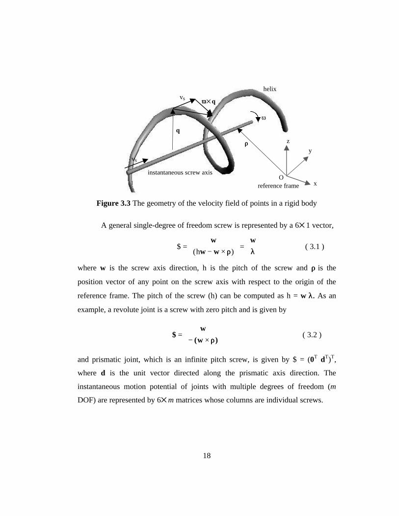
Figure 3.3 The geometry of the velocity field of points in a rigid body

A general single-degree of freedom screw is represented by a 651 vector,

$( )

=− ×

=

w

w w

w

h ρρ λλ( 3.1 )

where w is the screw axis direction, h is the pitch of the screw and ρρ is the

position vector of any point on the screw axis with respect to the origin of the

reference frame. The pitch of the screw (h) can be computed as h = w⋅⋅λ.λ. As an

example, a revolute joint is a screw with zero pitch and is given by

$( )

=− ×

w

w ρρ( 3.2 )

and prismatic joint, which is an infinite pitch screw, is given by $ = (0T dT)T,

where d is the unit vector directed along the prismatic axis direction. The

instantaneous motion potential of joints with multiple degrees of freedom (m

DOF) are represented by 65m matrices whose columns are individual screws.

helix

instantaneous screw axis

ω

vs

vs ωω5q

reference frame

q

ρρ

x

y

z

O

19

3.1.2 Motor ( $v )

While a screw is a purely geometric quantity, a motor is the representation

of spatial velocity of a rigid body. It can be obtained by multiplying the scalar

angular velocity about the screw axis with the screw vector. A motor about a

screw axis is a 651 vector and is represented by a pair of 351 vectors. The top

vector, referred to as ωω, is the angular velocity of motion about the screw axis.

The direction of the angular velocity is parallel to the screw axis. The lower

vector, referred to as µµ, is the linear velocity, produced by the screw motion about

the axis with angular velocity ωω, of the point in the rigid body which

instantaneously coincides with the origin of the reference frame: $v = (ωωT µµT)T =

ω$. In the case of a prismatic joint, ωω = 0 and µ µ = µd.

3.1.3 Wrench ( $f )

The geometric concept of screw is now extended to represent force

systems. A wrench, about a screw axis is a 651 vector and is represented by a

vector pair (FT, ττT)T where F is the resultant force of the force system represented

by the wrench and ττ is the corresponding resultant torque about the origin of the

reference frame.

3.1.4 Reciprocity

When two screws, $1 and $2, satisfy the following condition, they are said

to be reciprocal to each other.

($1)T Π Π $2 = 0 ( 3.3 )

where, ΠΠ = 0 3 I 3

I 3 0 3

03 I3I3 03

and I3 = 353 identity matrix. Between a motor and a

wrench system, this is the condition for the wrench to do no work if applied to a

20

body free to move about the screw axis of the motor [Hunt, 1990]. It should be

noted that Equation 3.3 is valid only between two screws one of which is a motor

and the other is a wrench. In fact the scalar product defined in Equation 3.3 is not

an inner product since it is possible to find non-zero, self-reciprocal screws (a

three dimensional pure force (no moment) applied through the center of a ball

joint represent a self-reciprocal situation).

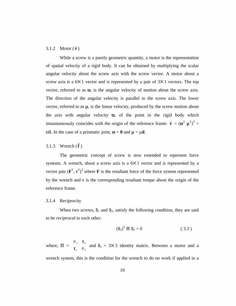
Figure 3.4 shows a rigid body connected to the ground by a ball joint and

two intersecting revolute joints. When the line of action of the wrench $f passes

through the intersecting point P and the center of the ball joint, the effect of $f

passes passively through the serial mechanism to the ground without performing

any work on the system. Therefore, the wrench $f is reciprocal to the motor

representing the motion of the serial mechanism of Figure 3.4.

For a system with m degrees of freedom, there is an instantaneous screw

system that is a vector space of order m that characterizes the rate kinematics of

the whole system. The reciprocal wrench system is a screw system of order 6-m.

Figure 3.4 A reciprocal wrench, $f , applied to a body with 5th order motion screw

It is important to note that screw systems are purely geometric quantities.

Therefore, the condition for the reciprocity is also purely a geometric relationship.

revolute joints

structural

elements line of action of the

reciprocal wrench toP

ball joint

$f

21

3.2 First Generation Orientation Stage

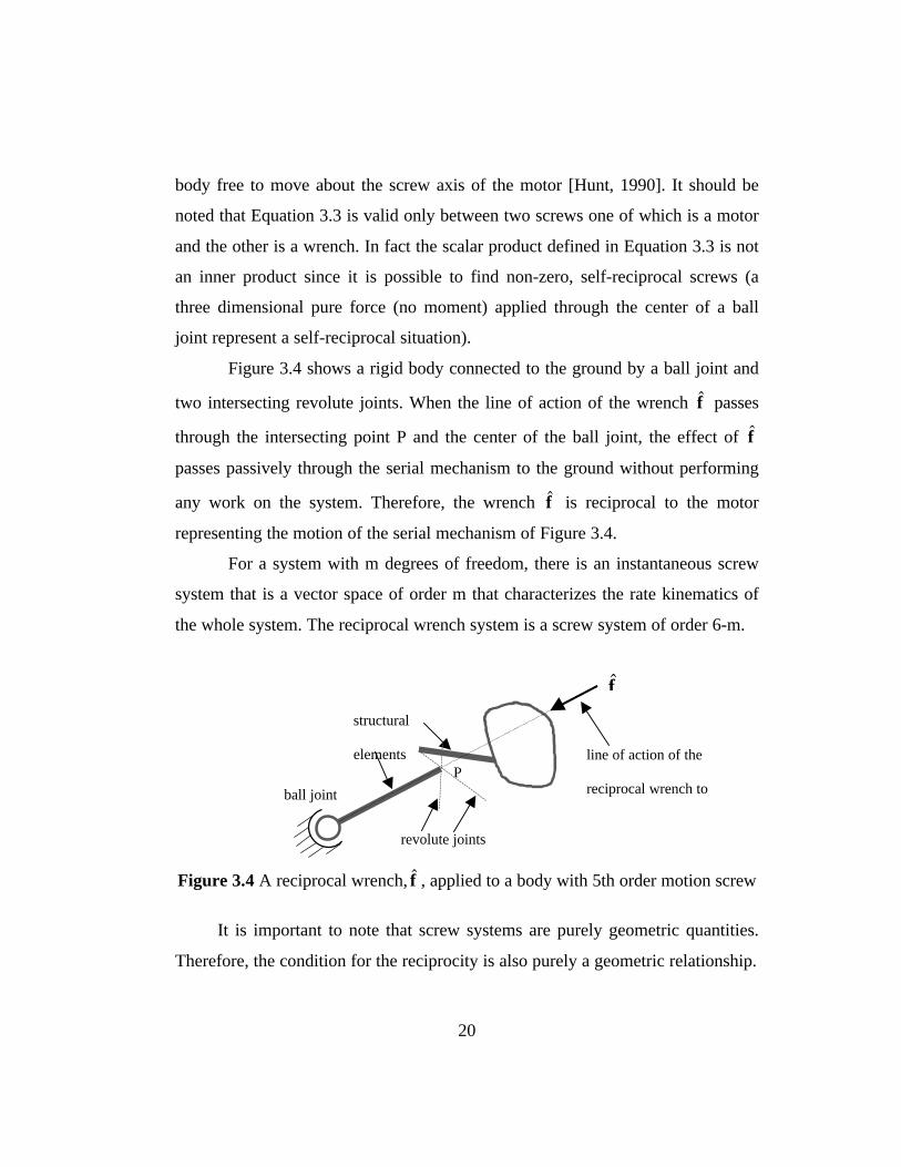
A literature search was the first step in developing the orientation stage.

Waldron, Raghavan, and Roth present a parallel linkage with three degrees of

freedom [Waldron,1989]. Figure 3.5 illustrates this linkage. Two equilateral

triangles are separated by three links. Each link consists of a ball joint, a

prismatic joint, and a revolute or pin joint. When the triangles are parallel, the

system is said to be in its nominal position, and its mobility corresponds to the

desired motions of α and β rotations and z translation as shown in the next

section.

Figure 3.5 Ideal orientation stage kinematic model

3.2.1 Mobility Analysis

To determine the motion capability of this mechanism, it is necessary to

find $m, the space of motors that describes the stage’s motion. This space can be

found by looking at the wrenches reciprocal to the mechanism. A reciprocal

wrench is a wrench that is transmitted through a linkage to ground without

causing the linkage to move. These reciprocal wrenches form a wrench space $f.

ball joint

prismaticjoint

revolutejoint

movingz

x y pi

22

The motion capability of the linkage is described by the motor space $m that is

reciprocal to $f. Thus, the following procedure may be used to identify $m:

1. Identify all wrenches if̂ reciprocal to the linkage

2. Identify the space $f spanned by all if̂

3. Identify the space $m that is reciprocal to $f

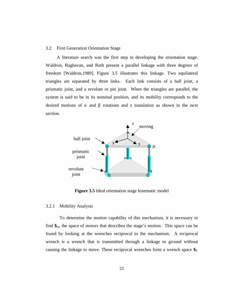
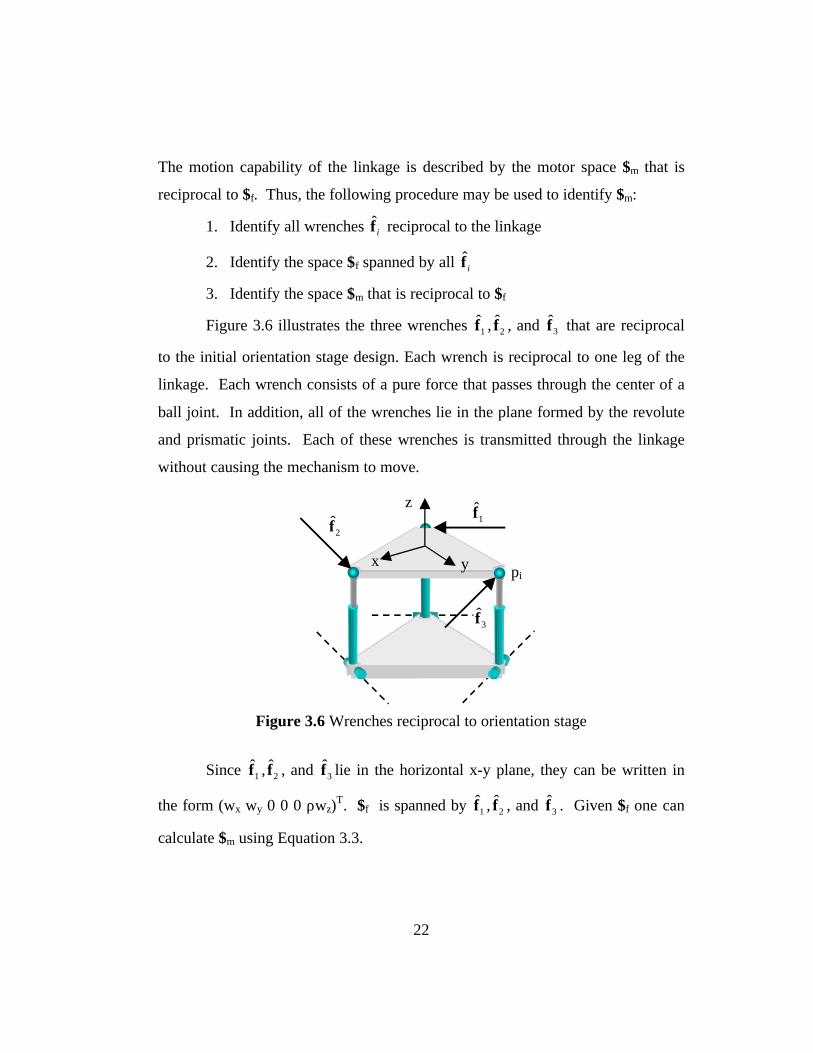
Figure 3.6 illustrates the three wrenches 1̂f , 2f̂ , and 3f̂ that are reciprocal

to the initial orientation stage design. Each wrench is reciprocal to one leg of the

linkage. Each wrench consists of a pure force that passes through the center of a

ball joint. In addition, all of the wrenches lie in the plane formed by the revolute

and prismatic joints. Each of these wrenches is transmitted through the linkage

without causing the mechanism to move.

Figure 3.6 Wrenches reciprocal to orientation stage

Since 1̂f , 2f̂ , and 3f̂ lie in the horizontal x-y plane, they can be written in

the form (wx wy 0 0 0 ρwz)T. $f is spanned by 1̂f , 2f̂ , and 3f̂ . Given $f one can

calculate $m using Equation 3.3.

z

x y pi

3f̂

1̂f2f̂

23

$f

=

1

0

0

0

0

0

,

0

0

0

0

1

0

,

0

0

0

0

0

1

span $m

=

1

0

0

0

0

0

,

0

0

0

0

1

0

,

0

0

0

0

0

1

span

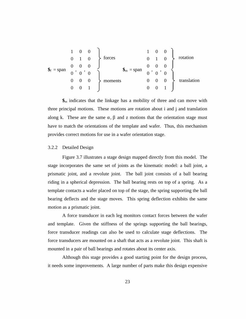
$m indicates that the linkage has a mobility of three and can move with

three principal motions. These motions are rotation about i and j and translation

along k. These are the same α, β and z motions that the orientation stage must

have to match the orientations of the template and wafer. Thus, this mechanism

provides correct motions for use in a wafer orientation stage.

3.2.2 Detailed Design

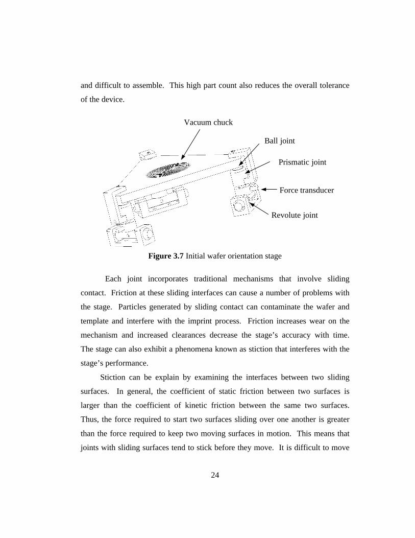
Figure 3.7 illustrates a stage design mapped directly from this model. The

stage incorporates the same set of joints as the kinematic model: a ball joint, a

prismatic joint, and a revolute joint. The ball joint consists of a ball bearing

riding in a spherical depression. The ball bearing rests on top of a spring. As a

template contacts a wafer placed on top of the stage, the spring supporting the ball

bearing deflects and the stage moves. This spring deflection exhibits the same

motion as a prismatic joint.

A force transducer in each leg monitors contact forces between the wafer

and template. Given the stiffness of the springs supporting the ball bearings,

force transducer readings can also be used to calculate stage deflections. The

force transducers are mounted on a shaft that acts as a revolute joint. This shaft is

mounted in a pair of ball bearings and rotates about its center axis.

Although this stage provides a good starting point for the design process,

it needs some improvements. A large number of parts make this design expensive

forces

moments

rotation

translation

24

and difficult to assemble. This high part count also reduces the overall tolerance

of the device.

Figure 3.7 Initial wafer orientation stage

Each joint incorporates traditional mechanisms that involve sliding

contact. Friction at these sliding interfaces can cause a number of problems with

the stage. Particles generated by sliding contact can contaminate the wafer and

template and interfere with the imprint process. Friction increases wear on the

mechanism and increased clearances decrease the stage’s accuracy with time.

The stage can also exhibit a phenomena known as stiction that interferes with the

stage’s performance.

Stiction can be explain by examining the interfaces between two sliding

surfaces. In general, the coefficient of static friction between two surfaces is

larger than the coefficient of kinetic friction between the same two surfaces.

Thus, the force required to start two surfaces sliding over one another is greater

than the force required to keep two moving surfaces in motion. This means that

joints with sliding surfaces tend to stick before they move. It is difficult to move

Ball joint

Prismatic joint

Revolute joint

Force transducer

Vacuum chuck

25

sliding joints through small displacements because they tend to move in finite

increments between locations where they stick. Problem with stiction, particle

generation and wear motivated a search for other orientation stage designs.

3.3 The Use of Flexures in Mechanism Design

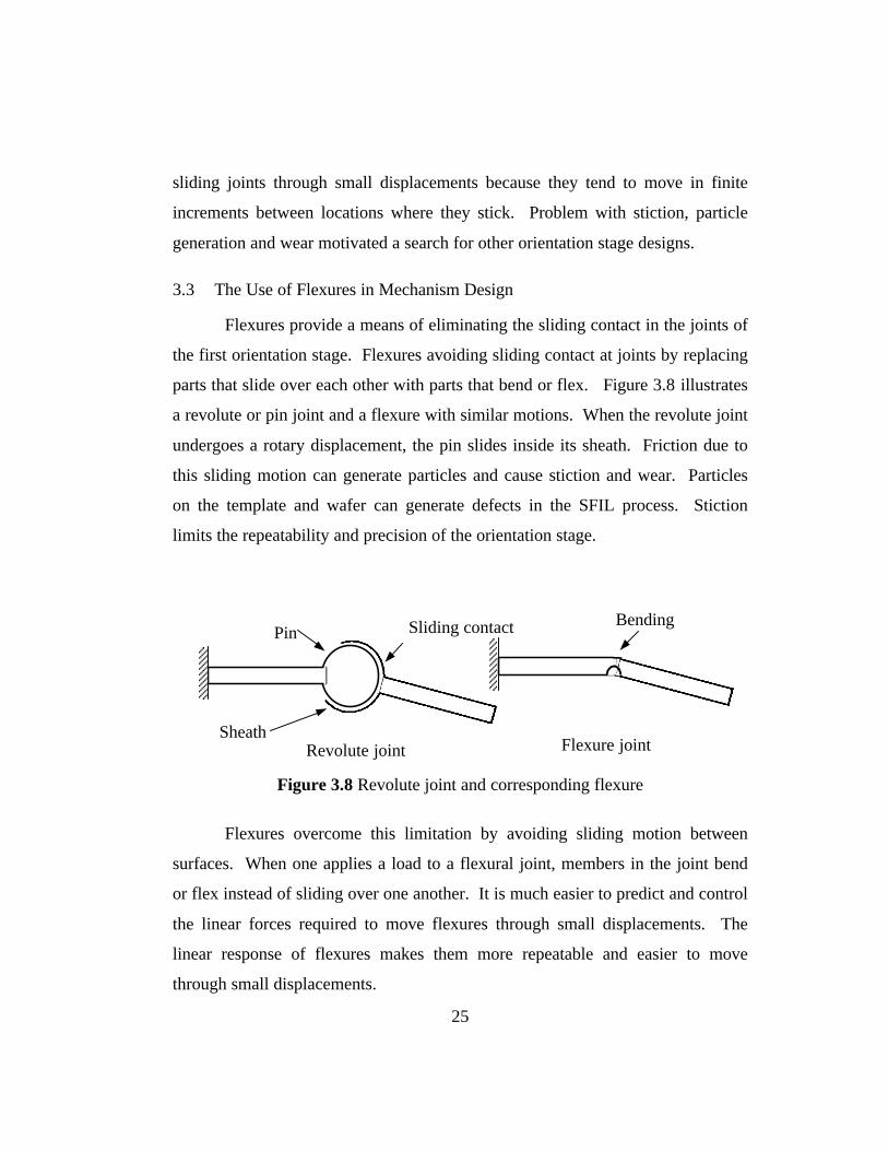
Flexures provide a means of eliminating the sliding contact in the joints of

the first orientation stage. Flexures avoiding sliding contact at joints by replacing

parts that slide over each other with parts that bend or flex. Figure 3.8 illustrates

a revolute or pin joint and a flexure with similar motions. When the revolute joint

undergoes a rotary displacement, the pin slides inside its sheath. Friction due to

this sliding motion can generate particles and cause stiction and wear. Particles

on the template and wafer can generate defects in the SFIL process. Stiction

limits the repeatability and precision of the orientation stage.

Figure 3.8 Revolute joint and corresponding flexure

Flexures overcome this limitation by avoiding sliding motion between

surfaces. When one applies a load to a flexural joint, members in the joint bend

or flex instead of sliding over one another. It is much easier to predict and control

the linear forces required to move flexures through small displacements. The

linear response of flexures makes them more repeatable and easier to move

through small displacements.

Sliding contact Bending

Revolute joint Flexure jointSheath

Pin

26

The absence of sliding contact also increases the lifetime of devices

constructed with flexures. Without sliding friction, wear in the mechanism is

significantly reduced if not eliminated. One must consider fatigue of flexing

joints when predicting a mechanism’s service life, but friction and wear effects

are minimized.

Flexures exhibit another desirable attribute for high precision equipment.

They exhibit no backlash due to clearances. A traditional pin joint such as the one

illustrated in Figure 3.8 normally has a slight gap between the pin and the sheath

it rests inside. This gap causes a phenomenon known as backlash where, in

addition to rotating, the pin moves from side to side inside the sheath. This

movement decreases the overall precision and repeatability of the stage.

Roller bearings or ball bearings also offer a means to avoid sliding

contact, stiction, and backlash. These devices replace sliding contact with rolling

contact. Surfaces in rolling contact experience no sliding friction. Thus, they

generate fewer particles and exhibit no stiction effects. Ball and roller bearings

may also be preloaded to avoid backlash.

The main difference between flexures and bearings is evident upon an

examination of their relative ranges of motion. When flexures are displaced,

elements in the joints undergo strain. The range of motion and lifetime of a

flexure is most often determined by the amount of strain and fatigue the flexural

elements can withstand. Bearings normally have an unlimited range of travel, and

their lifetime is usually determined by the wear of elements in contact. A final

factor to consider when determining whether to use bearings or flexures is the size

of the joint. Small compact linkages often require small compact joints. Bearings

consist of many parts and cannot be manufactured as small as flexures. Bearings

can significantly increase the size and mass (and thus, reduce the natural

frequency) of a linkage. Flexures offer a stiff, lightweight means of

27

manufacturing joints that are free of stiction, particle generation, and wear due to

sliding contact.

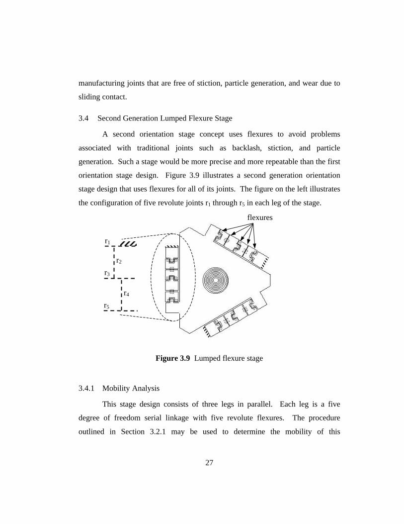
3.4 Second Generation Lumped Flexure Stage

A second orientation stage concept uses flexures to avoid problems

associated with traditional joints such as backlash, stiction, and particle

generation. Such a stage would be more precise and more repeatable than the first

orientation stage design. Figure 3.9 illustrates a second generation orientation

stage design that uses flexures for all of its joints. The figure on the left illustrates

the configuration of five revolute joints r1 through r5 in each leg of the stage.

Figure 3.9 Lumped flexure stage

3.4.1 Mobility Analysis

This stage design consists of three legs in parallel. Each leg is a five

degree of freedom serial linkage with five revolute flexures. The procedure

outlined in Section 3.2.1 may be used to determine the mobility of this

flexures

r1

r2

r3

r4

r5

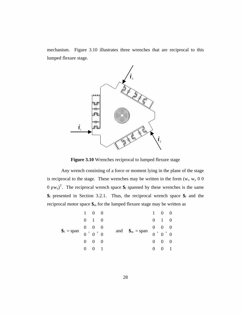
28

mechanism. Figure 3.10 illustrates three wrenches that are reciprocal to this

lumped flexure stage.

Figure 3.10 Wrenches reciprocal to lumped flexure stage

Any wrench consisting of a force or moment lying in the plane of the stage

is reciprocal to the stage. These wrenches may be written in the form (wx wy 0 0

0 ρwz)T. The reciprocal wrench space $f spanned by these wrenches is the same

$f presented in Section 3.2.1. Thus, the reciprocal wrench space $f and the

reciprocal motor space $m for the lumped flexure stage may be written as

$f

=

1

0

0

0

0

0

,

0

0

0

0

1

0

,

0

0

0

0

0

1

span and $m

=

1

0

0

0

0

0

,

0

0

0

0

1

0

,

0

0

0

0

0

1

span

3f̂

1̂f

2f̂

29

Again, $m indicates that the linkage has a mobility of three and can move

with three principal motions. These motions are rotation about i and j and

translation along k. These are the same α, β and z motions that the orientation

stage must have to match the orientations of the template and wafer.

3.4.2 Detailed Design

The lumped flexure stage design incorporates many improvements over

the first stage design. As previously mentioned, this stage design eliminates

backlash, particle generation, and stiction through the use of flexures. This design

also illustrates an alternative geometry that yields the same desired third order

mobility as the first orientation stage design. Although the stages have similar

numbers of parts, the second stage features a less intricate design and would be

simpler to construct and assemble.

However, a few features of the lumped flexure design leave room for

improvement. This stage achieves its three degree of freedom mobility by linking

three serial arms to one body. Each of the legs uses commercially available

revolute flexures. These flexures, however, were to compliant, and the stage

design was not stiff enough. When designing highly repeatable and precise

mechanisms, one should try to design mechanisms with high stiffnesses and

natural frequencies. If a mechanism’s fundamental natural frequency is greater

than 500 Hertz, the mechanism will be less sensitive to environmental vibrations

of frequencies up to 200 Hertz. This design is too compliant and would be very

sensitive to environmental vibration.

3.5 Third Generation Distributed Flexure Stage

A third generation orientation stage design provides to improvements based

on the lessons learned in the second stage design. Specifically, the design

30

incorporates the advantages of flexures into a simple compact design with few

parts. Further investigation of work in the field of precision engineering produced

a mechanism built by Badami, Smith, and Patterson that was used to monitor tilt

misalignments with stylus probes [Badami, 1996]. This device uses a flexure

ring to achieve three degrees of freedom. Some modifications and adjustments to

this design yielded the third wafer orientation stage design. Figure 3.11 illustrates

this distributed flexure stage.

Figure 3.11 Distributed flexure orientation stage

This device derives its motion capability from an aluminum distributed

flexure ring. This flexure ring supports a vacuum chuck in the center of the stage.

When a template contacts a wafer on the orientation stage, the template generates

a moment about the center of the stage. This moment deflects the aluminum ring

supporting the vacuum chuck. The circular symmetry of the ring allows the wafer

to match the orientation of the template while minimizing lateral motion between

the template and wafer.

Aluminum flexure ringVacuum chuck

31

Beam approximations were used to determine appropriate dimensions for

the flexure ring. Each third of the flexure ring was modeled as a straight fixed-

fixed beam. Figure 3.12 and Equation 3.4 describes the behavior of a fixed-fixed

beam under a load [Gere, 1990].

Figure 3.12 Fixed-fixed beam

12

192 3

3

bhI

L

EIF =∂= ( 3.4 )

where

F = force required to deflect beam

E = Young’s Modulus of beam material

I = moment of inertia of beam

L = length of beam

b = width of beam

h = height of beam

Equation 3.4 was used to estimate the forces required to deflect a beam.

To correct for a few degrees of angular misalignment, the flexure ring is designed

so that each segment of the ring deflects roughly 2 mm under a 66 N (15 lb.) load.

The ring is made of 7075-T6 aluminum (E = 72 GPa). According to Equation

L

F

b

h

32

3.4, a 7075-T6 aluminum beam of length L =135 mm, base of b = 14.5 mm, and

height of h = 1.27 mm will deflect 2 mm under a 28 N (6.3 lb) load. The beam

can experience four times the stress due to this deflection before it deforms

plasticly. A flexure ring of these dimensions would deflect roughly 2 mm under

an 84 N (18.9 lb) load. The flexure ring incorporated into the distributed flexure

stage is based on these dimensions.

This stage design incorporates the advantages of flexures and avoids

sliding contact that is present in traditional joints. Its simplistic design uses a

small number of parts and can be assembled quickly. This design also presents an

interesting kinematic analysis question. There is some question about how to

model and analyze the motion capability of a distributed flexure device. Chapter

4 presents a framework for answering these questions and compares the motion

capabilities of the ideal three leg kinematic model and the distributed flexure

stage.

33

4 Mobility Analysis

The distributed flexure stage presented in Section 4.3 poses an interesting

analysis problem: What is the best way to determine the principal motion

capabilities of a mechanism incorporating distributed compliance? Smith and

Chetwynd have shown how beam approximations may be used to model

individual flexure element [Smith, 1992]. Smith has shown how to approximate

the motion of a cantilever flexure as a revolute joint. This chapter presents a

system level analysis that looks at a generalized compliance matrix. A finite

element model is used to compute the non-ideal compliance matrix of the

distributed flexure stage. The results of the finite element model are then used to

examine the stage’s principal motion capabilities.

4.1 Basis of Comparison

Patterson and Lipkin present a format for investigating the motion

capabilities of compliant structures [Patterson, 1993]. A rigid body fully

supported by an elastic system has six degrees of freedom. The motion

capabilities of the rigid body may be determined by examining the elastic

structure supporting the body. For example, the motion capability of the vacuum

chuck in the distributed flexure stage may be determined by examining the

compliant structure of the aluminum flexure ring. Similarly, the motion

capability of the top plate of the ideal kinematic model presented in Section 3.2

may be determined by examining the kinematic structure supporting the plate.

4.1.1 Wrenches, Twists, and the Compliance Matrix

Screw theory offers a means of quantifying the motion capability of a

compliant structure. A wrench, f̂ , and twist, T̂ , may be used to describe the

34

motion of a rigid body supported by an compliant structure. A wrench in ray

coordinates, [ ]TTTf τrr

=f̂ , consists of a force, fr

, and a moment, τr

, about a

screw axis. A twist in axis coordinates, [ ]TTT γrr

∂=T̂ represents a small

displacement about a screw axis. ∂r

represents a linear deflection and

γr

represents a rotational deflection about a screw axis. A compliance matrix C

relates a wrench to a twist:

fCT ˆˆ = ( 4.1 )

The ΠΠ operator may be used to convert a twist in axis coordinates, T̂ , to a

twist in ray coordinates, t̂ :

ΠΠ t̂ = T̂ ( 4.2 )

where

Π = Π =

0I

I0

Equation 4.1 and Equation 4.2 may be combined to relate f̂ and t̂ :

=t̂ Π Π C f̂ ( 4.3 )

By assuming that the wrench f̂ and twist t̂ are scalar multiples of the same

screw, it is possible to construct an eigenvalue problem:

λ λ e = ΠΠ C e ( 4.4 )

This formulation yields six eigenvalues λλi and six eigenvectors or

eigenscrews ei. λλi represents the ratio of angular deformation to force (λλ = γ / f ).

The eigenvectors ei are known as eigenscrews in ray coordinates. It is assumed

that twists are small displacements about an equilibrium position and that they can

35

be represented as a vector in R6. A wrench applied about a given eigenscrew ei

produces a twist about the same eigenscrew ei [Patterson, 1993]. Note that

Equation 4.4 solves the eigenvalue problem for the matrix ΠΠC. The eigenvalues

of C are frame dependent and the resulting eigenvectors do not provide physically

meaningful approximation of the motion capabilities of spatial mechanisms.

These eigenscrews of ΠΠC represent the fundamental modes of a compliant

mechanism. The eigenscrews represent the directions in which the mechanism

can be displaced in a decoupled manner, and the eigenvalues represent the angular

deflection about an eigenscrew for an applied wrench. All of the motions of a

compliant mechanism may be modeled as linear combinations of the fundamental

eigenscrews.

Note that eigenvalues and eigenvectors of the matrix ΠΠC are invariant with

respect to the transformation from ray coordinates to axis coordinates. An

analysis in ray coordinates yields the same set of eigenvalues and eigenscrews as

an analysis in axis coordinates [Patterson, 1993]. Determining the compliance

matrix for a partially constrained elastic structure provides a means to examine its

motion capability by looking at the eigenscrews of the compliance matrix. For

this reason, eigenvalues and eigenscrews provide an attractive tool for comparing

the motions of partially constrained compliant mechanisms.

Eigenscrews with zero eigenvalues can be examined to gain some insight

into the motion capability of a partially constrained mechanism. The space

spanned by all eigenscrews with zero eigenvalues is equal to the space spanned by

all wrenches reciprocal to the mechanism. One can find the space spanned by a

mechanism’s reciprocal wrenches by finding the space spanned by eigenscrews of

the ππC matrix with eigenvalues equal to zero.

Sections 4.2 and 4.3 compare the motion capabilities of the three leg ideal

kinematic model and the distributed flexure stage. Section 4.2 presents an

36

analytical derivation of the ideal kinematic stage’s compliance matrix and its

eigenvalues and eigenscrews. Section 4.3 presents the finite element model used

to determine the distributed flexure stage’s compliance matrix. The eigenscrews

and corresponding eigenvalues of the stage are also presented. Section 4.4

compares the motion capabilities of the two mechanisms and presents some a

summary of this chapter.

4.2 Ideal Kinematic Stage

This section examines the motion capability of the three leg stage. By

treating each of the prismatic joints as a spring with a finite compliance, one can

compute the resulting small displacement of the stage about an equilibrium point

for a given wrench. This section presents an analytical derivation of the

compliance matrix of the three leg kinematic model. The eigenvalues and

eigenscrews of the compliance matrix are then examined to provide insight into

the model’s motion capabilities.

4.2.1 Compliance Matrix

The derivation of the model’s compliance matrix begins with an

examination of the six screws that span the space of all possible motors of the

mechanism. Figure 4.1 illustrates these screws. 1$ , 2$ , and 3$ represent the

motions that the stage can move in. When the stage is loaded, its movement will

be a linear combination of motors represented by 1$ , 2$ , and 3$ . r1$ , r$ , and r

3$

represent the screws reciprocal to the system. A wrench applied along these

screws will be transmitted through the linkage and cause no movement.

37

Figure 4.1 Screw representation of three leg model

These six screws can be assembled into an operator that maps a general

wrench applied to the system into reciprocal and non-reciprocal components.

This operator is known as the Jacobian, J:

J = [ 1$ 2$ 3$ r1$ r

2$ r3$ ] ( 4.5 )

An applied wrench may be separated into its reciprocal and non-reciprocal

components using the Jacobian:

J [ 1f 2f 3f r1f r

2f r3f ]T = bf ( 4.6 )

where bf represents a wrench applied to the top surface of the system, 1f , 2f , and

3f represent forces in the prismatic joints, r1f , r

2f , and r3f represent wrenches

reciprocal to the linkage.

Motions of the linkage can be examined using these six screws. The

velocity of the three corners, P1, P2, and P3 of the top plate, may be related to the

velocity of, b, the center of the top plate:

ibbb

P pVi

×+= ωµ ( 4.7 )

r2$

z

x y pi

r1$

r3$

1$ 2$

3$

b

38

where

iPV = velocity of point P

µb = velocity of top plate in frame b

ωb = angular velocity of top plate in frame b

ip = location of point Pi in frame b

By assuming that Pi moves only a small distance along the direction of the

screw, the displacement of PI can be determined:

( )ibbb

ib

i pw ×+⋅=∂ ωµ ( 4.8 )

where

i∂ = small displacement of Pi

ib w = direction vector of Screw $i

Equation 4.8 may be rewritten to express i∂ in screw notation:

( )[ ]

×=∂

ωµ

b

bT

ib

ib

ib

i wpw

=∂

µω

πb

bTii $ ( 4.9 )

The displacements of points Pi along the six screws i$ and ri$ may be

related to the overall twist t̂ of the plate:

( ) tÐJ ˆ321321

TTrrr =∂∂∂∂∂∂ ( 4.10 )

Any displacement i∂ may be related to the force fi along a spring via the

spring’s compliance. The set of six displacements may be related to the set of six

spring forces:

39

∂∂∂∂∂∂

=

=

=∆=∆

r

r

r

r

r

r

f

f

f

f

f

f

c

c

c

3

2

1

3

2

1

3

2

1

3

2

1

3

2

1

ˆˆ

00000

00000

00000

000000

000000

000000

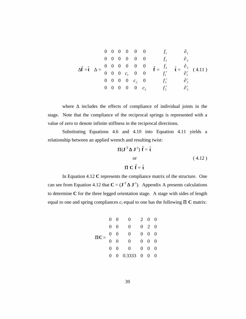
ˆˆ tftf ( 4.11 )

where ∆ includes the effects of compliance of individual joints in the

stage. Note that the compliance of the reciprocal springs is represented with a

value of zero to denote infinite stiffness in the reciprocal directions.

Substituting Equations 4.6 and 4.10 into Equation 4.11 yields a

relationship between an applied wrench and resulting twist:

ΠΠ(J-T ∆ ∆ J-1) f̂ = t̂

or ( 4.12 )

Π Π C f̂ = t̂

In Equation 4.12 C represents the compliance matrix of the structure. One

can see from Equation 4.12 that C = (J-T ∆ ∆ J-1). Appendix A presents calculations

to determine C for the three legged orientation stage. A stage with sides of length

equal to one and spring compliances ci equal to one has the following Π Π C matrix:

ΠΠC

=

0003333.000

000000

000000

000000

020000

002000

40

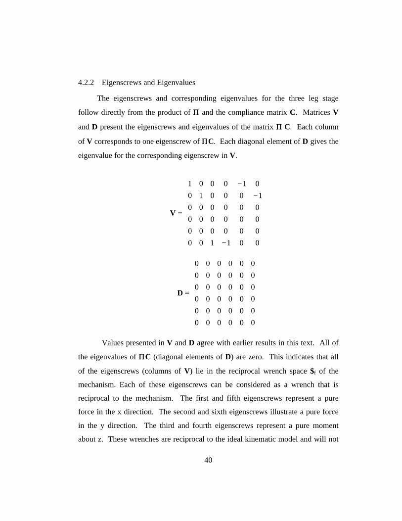
4.2.2 Eigenscrews and Eigenvalues

The eigenscrews and corresponding eigenvalues for the three leg stage

follow directly from the product of ΠΠ and the compliance matrix C. Matrices V

and D present the eigenscrews and eigenvalues of the matrix Π Π C. Each column

of V corresponds to one eigenscrew of ΠΠC. Each diagonal element of D gives the

eigenvalue for the corresponding eigenscrew in V.

−

−−

=

001100

000000

000000

000000

100010

010001

V

=

000000

000000

000000

000000

000000

000000

D

Values presented in V and D agree with earlier results in this text. All of

the eigenvalues of ΠΠC (diagonal elements of D) are zero. This indicates that all

of the eigenscrews (columns of V) lie in the reciprocal wrench space $f of the

mechanism. Each of these eigenscrews can be considered as a wrench that is

reciprocal to the mechanism. The first and fifth eigenscrews represent a pure

force in the x direction. The second and sixth eigenscrews illustrate a pure force

in the y direction. The third and fourth eigenscrews represent a pure moment

about z. These wrenches are reciprocal to the ideal kinematic model and will not

41

cause it to move. The reciprocal wrench space $f of dimension three is spanned

by these six eigenscrews.

Equation 3.3 provides a means of determining the motor space $m that is

reciprocal to $f :

($f)T Π Π $m = 0

thus,

=

0

1

0

0

0

0

,

0

0

1

0

0

0

,

0

0

0

1

0

0

spanm$

$m indicates that the stage can translate in the z direction and rotate about

the x and y axes. This analysis agrees with the work presented in Section 3.2.1

that examined the motion capability of the three leg kinematic model. Both

analyses found that the ideal model could translate along the z axis and rotate

about the x and y axes.

It is interesting to note that the ΠΠC matrix since its eigenvectors do not span

the six-dimensional space [Strang, 1997]. In fact, they only span the three-

dimensional reciprocal space. It is well-known in the linear algebra literature that

repeated eigenvalues are a pre-requisite for a defective eigenvector space. The

eigenvalues of non-ideal stages that have very similar but not identical

compliance characteristics as an ideal stage are not likely to be exactly zero. This

leads to a case where a near defective matrix possesses six linearly independent

eigenvectors. As shown in the following analysis, a careful formulation of the

problem is required to allow effective comparisons between ideal and near-ideal

stages.

42

4.3 Distributed Flexure Stage

The distributed flexure stage design presents an interesting analysis

problem: given a rigid body supported by an elastic suspension, how is the rigid

body’s motion capability determined? This section presents a finite element

analysis (FEA) of the distributed flexure stage. Data generated from the FEA

model is used to determine the structure’s compliance matrix. A discussion of the

eigenvalue problem for the FEA determined compliance matrix concludes the

section.

4.3.1 Finite Element Model

The first step in determining the motion capability of the distributed flexure

stage is to compute the stage’s compliance matrix. The fact that the distributed

flexure stage derives its motion capability from an aluminum flexure ring makes

analysis difficult. Traditional methods of computing compliance matrices, such

as the one used to determine the compliance matrix of the ideal stage, rely on the

geometry of a mechanism and the location of all of its joints. The lack of well-

defined joints in the distributed flexure stage makes it difficult to apply these

methods. The movement of the flexure would have to be approximated with the

movement of individual joints. This process of approximating the flexure’s

movement quantizes the distributed compliance of the stage and treats it as a

group of lumped compliances or joints.

A finite element model provides an alternative means of generating a

structure’s compliance matrix. Finite element codes allow the user to compute

the deflection of a compliant mechanism for a given load. If one knows the

deflection of a compliant mechanism for six linearly independent wrenches, one

can compute the mechanism’s compliance matrix:

F ΠΠC = T ( 4.13 )

43

ΠΠC = T F-1 ( 4.14 )

where

F = 6 x 6 matrix of six applied wrenches if̂

T = 6 x 6 matrix of corresponding twists it̂

C = 6 x 6 compliance matrix

A finite element model allows a user to model the behavior of a compliant

mechanism without having to construct and test the device. Because FEA

simulates structures based on the geometry and structure of the entire compliant

mechanism, it yields results comparable to those of an actual stage. The

comparison of these FEA results to the motions of the ideal model is a key

element of this work.

Figure 4.2 illustrates the finite element model used to analyze the

distributed flexure stage. IDEAS master series 5.0 software was used to create

the finite element model of the distributed flexure stage. Part geometry

simulating the flexure ring and vacuum chuck was generated in Pro/Engineer

version 20 and exported to IDEAS using an IGES format. The part was then

meshed using a free mesh generator in IDEAS. The meshed part contained 817

elements and 2039 nodes.

ray coordinates

44

Figure 4.2 Finite element model

Boundary conditions are defined to allow no linear or rotational

displacement at the three locations where the flexure ring connects to the base.

These conditions simulate a rigid structure supporting the flexure ring.

Six linearly independent wrenches were applied to the structure. Each

column of matrix F represents a wrench applied to the FEA model. The top three

elements of every wrench denote linear forces. The lower three elements of every

wrench denote moments applied about the center of the vacuum chuck. The first

three columns represent forces applied at the center of the vacuum chuck along

the x, y, and z axes. The last three columns represent moment generating forces

applied at locations other than the center of the vacuum chuck.

F =

−−

−−−

6.3622.18400000

005.1416000

7962.11.1240000

0007.6600

7.667.66007.660

007.66007.66

Flexure ring

Vaccum chuck

Fixed boundaryconditions

forces

moments

45

The finite element model computes a deflection for every individual

applied wrench. Figure 4.3 illustrates the finite element model computation of the

stage’s deflection under a vertical load (second column of F). The undeformed

model is shown as a black wireframe, and the deformed model is shown as a

shaded contour plot. Shading indicates von Mises stresses in the structure as it

deforms.

Figure 4.3 Deflected finite element model

The finite element model outputs the deflection of the stage as a set of

node deflections. Waldron outlines a method for relating initial and final

locations of three points on a rigid body that undergoes a displacement to an

equivalent screw displacement [Waldron, 1993]. This method was used to

convert the nodal displacements of three points on the vacuum chuck to a

corresponding screw displacement. By assuming small displacements, these

screws are represented as twist vectors. Appendix B presents a MATLAB file

that details these calculations. Matrix T presents the twists corresponding to each

wrench in matrix F. Each column T represents the twist due to the wrench

represented by the corresponding column of F.

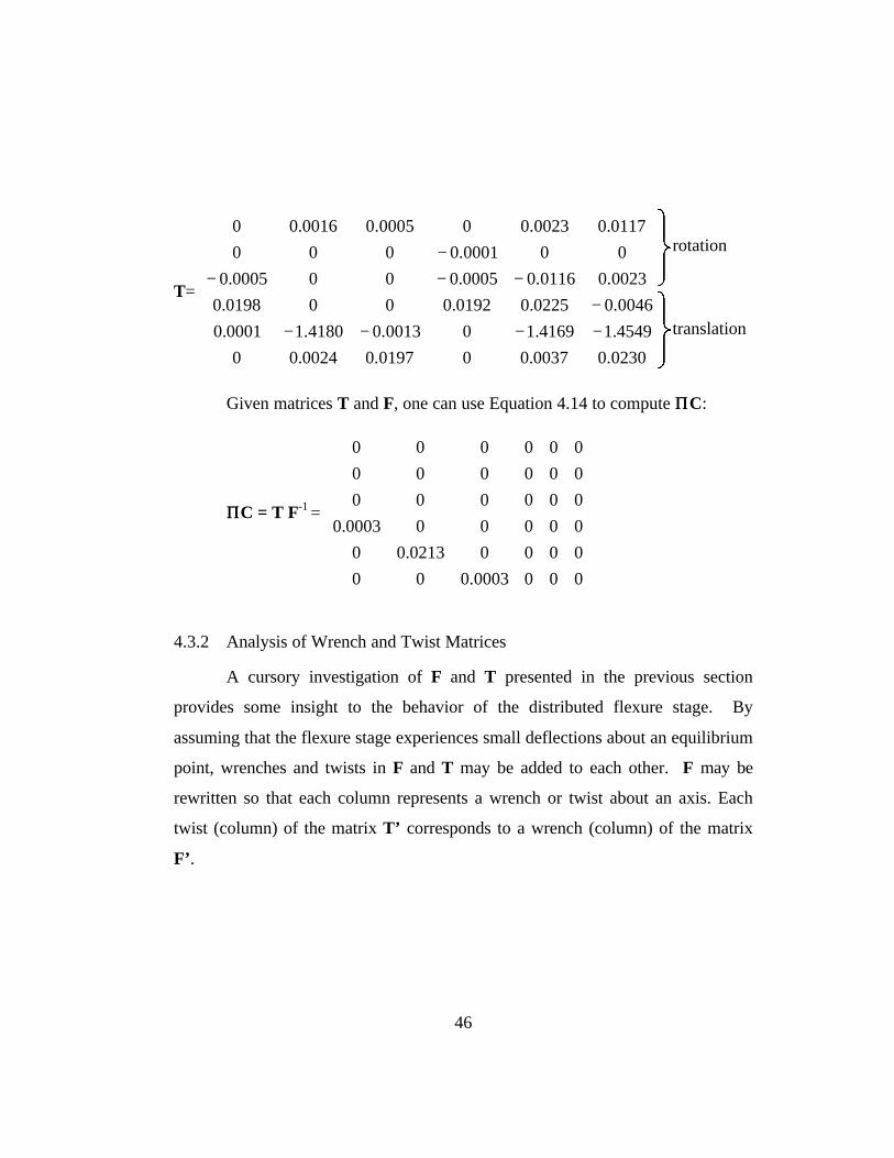
46

T=

−−−−−

−−−−

0230.00037.000197.00024.00

4549.14169.100013.04180.10001.0

0046.00225.00192.0000198.0

0023.00116.00005.0000005.0

000001.0000

0117.00023.000005.00016.00

Given matrices T and F, one can use Equation 4.14 to compute ΠΠC:

ΠΠC = T F-1

=

0000003.000

00000213.00

000000003.0

000000

000000

000000

4.3.2 Analysis of Wrench and Twist Matrices

A cursory investigation of F and T presented in the previous section

provides some insight to the behavior of the distributed flexure stage. By

assuming that the flexure stage experiences small deflections about an equilibrium

point, wrenches and twists in F and T may be added to each other. F may be

rewritten so that each column represents a wrench or twist about an axis. Each

twist (column) of the matrix T’ corresponds to a wrench (column) of the matrix

F’.

rotation

translation

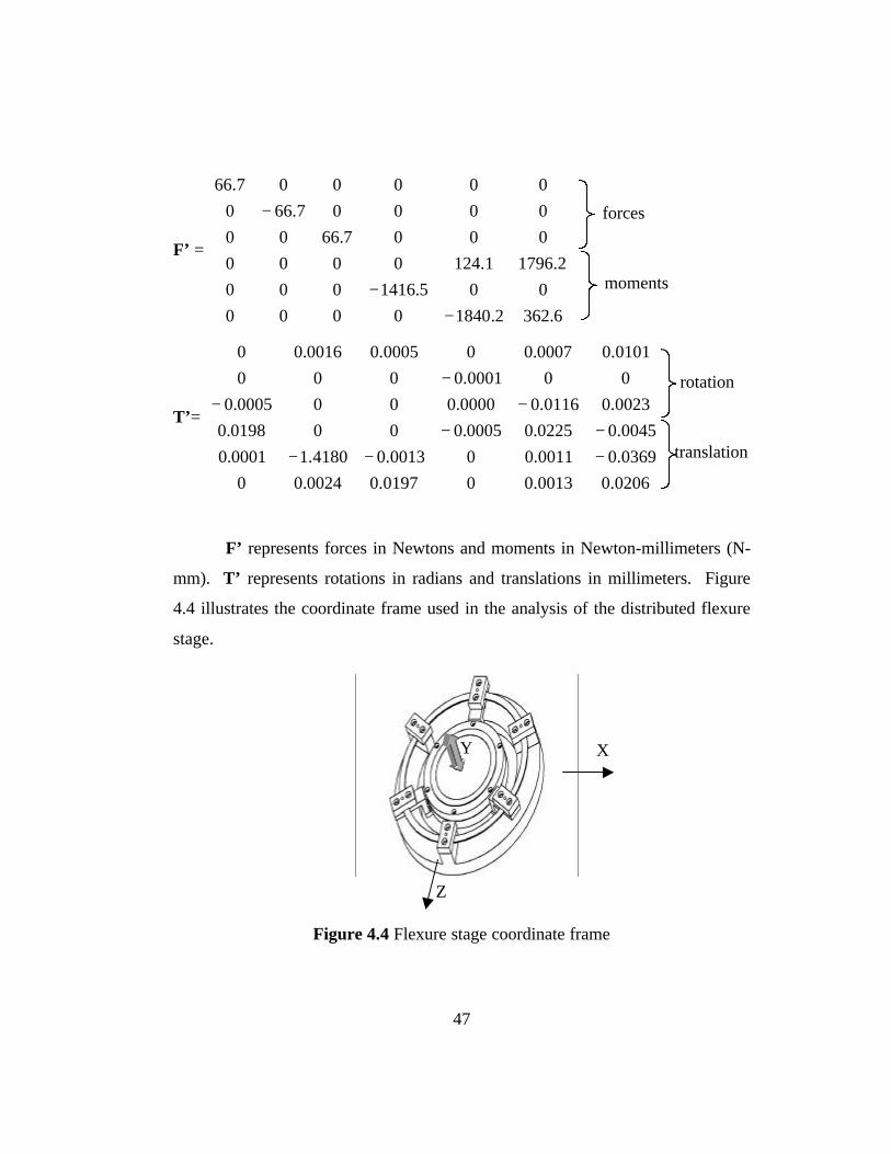
47

F’ =

−−

−

6.3622.18400000

005.1416000

2.17961.1240000

0007.6600

00007.660

000007.66

T’=

−−−−−

−−−

0206.00013.000197.00024.00

0369.00011.000013.04180.10001.0

0045.00225.00005.0000198.0

0023.00116.00000.0000005.0

000001.0000

0101.00007.000005.00016.00

F’ represents forces in Newtons and moments in Newton-millimeters (N-

mm). T’ represents rotations in radians and translations in millimeters. Figure

4.4 illustrates the coordinate frame used in the analysis of the distributed flexure

stage.

Figure 4.4 Flexure stage coordinate frame

Y X

Z

forces

moments

rotation

translation

48

The information contained in F’ and T’ describes the resulting twists ti for

a set of six linearly independent wrenches fi. f1 represents a 66.7 N (15 lb.) force

applied along the x axis. t1 indicates that the stage undergoes a –0.0005 radian

(0.03 degree) rotation about the y axis and translates 0.02 mm along the x axis.

f2 represents a -66.7 N (-15 lb.) force applied along the y axis. t2 indicates

that the stage undergoes a 0.0016 radian (0.09 degree) rotation about the x axis

and translates 1.4 mm down the y axis.

f3 represents a 66.7 N (-15 lb.) force applied along the z axis. t3 indicates

that the stage undergoes a 0.0005 radian (0.03 degree) rotation about the x axis

and translates 0.02 mm along the z axis.

The remaining moment-twist pairs may be interpreted in a similar manner.

f5 denotes a wrench dominated by a –1840 Nmm moment about the z axis. The

corresponding twist t5 indicates a –0.0116 radian (0.66 degree) rotation about the

z axis and 0.001, 0.02, and 0.001 mm translations along the x, y, and z axes

respectively. Thus, a 0.66 degree rotation about the z axis induces a 0.0001 mm

translation along the x and z axes.

Note that the stage is compliant about the x and z axes and along the y

axis. The stage is most likely to rotate about x and z and translate in z. This

initial analysis indicates that the flexure stage’s motion capability is very similar

to the ideal stage’s motion capability. However, these results depend on the

coordinate frame used and the applied moments selected. The following section

looks for a frame invariant analysis method based on the eigenvalues and

eigenvectors of the ΠΠC matrix.

4.3.3 Eigenvalues and Eigenvectors

Given the ΠΠC matrix presented in Section 4.3.1, it is possible to draw some

conclusions about the motion capability of the flexure stage. Eigenvectors with

49

zero eigenvalues identify wrenches that are reciprocal to the mechanism. While

this analysis works well for ideal compliance matrices such as the one presented

in Section 4.2.1, the eigenvalue analysis of a non-ideal compliance matrix is less

straightforward.

Lipkin, et. al. have produced a significant body of work dealing with this

eigenvalue problem [Patterson, 1993]. They limit the scope of their work,

however, to compliant structures with six degrees of freedom. These

unconstrained structures always have eigenvector space of rank six. Constrained

compliant structures with fewer than six degrees of freedom have a deficient

eigenvector space with a rank less than six. For example, the ideal kinematic

model presented earlier in this text is constrained to move with only three degrees

of freedom (it has three springs that can deflect). The ideal model has three

linearly independent eigenvectors, so the rank of the space spanned by its

eigenvectors is three. The ideal stage does not have a complete set of six linearly

independent eigenvectors, so it is said to have a deficient eigenvector space.

A deficient eigenvector space by itself does not create a problem with the

eigenvalue analysis of a compliance matrix. Difficulties arise, however, if

attempts are made to solve the eigenvalue problem for the compliance matrix of a

near-ideal stage that has been numerically derived. The finite element model

derivation of the distributed flexure stage’s compliance matrix is such a case. The

flexure stage’s compliance matrix is both numerically derived and has a deficient

eigenvector space. Solving for the eigenvalues and eigenvectors of ΠΠC for the

distributed flexure stage yields a set of distinct eigenvalues and spurious

eigenvectors. These eigenvectors cannot be interpreted to gain insight into a

physical system’s behavior.

This eigenvalue problem breaks down because the compliance matrix has

been numerically computed and it has a deficient eigenvector space. A

50

compliance matrix with a deficient eigenvector space that is computed directly

from geometry, has a set of some zero and some non-zero eigenvalues.

Eigenvectors with zero eigenvalues represent wrenches reciprocal to the system.

However, since the compliance matrix was numerically computed, one cannot

solve for exact eigenvalues. The eigenvalues of the numerically computed

compliance matrix are small, but they are not equal to zero. The matrix D

represents the eigenvalues of the ΠΠC matrix of the flexure stage. V lists the

eigenvectors corresponding to the eigenvalues presented in D.

D=

−

−+

−−+−

65.400000

065.40000

0017.008.4000

00017.008.400

000018.008.40

0000018.008.4

i

i

i

i

E-5

V=

+−++−+−−−−−−−+−

+++−−+−−+−

iii

iii

iii

i

iii

iii

106.0009.0099.0009.0099.0009.0

395.0049.0278.0090.0278.0090.0

057.0105.0076.0102.0076.0102.0

456.7059.27.239i 0.9377.239i -0.937

318.0096.0260.0044.0260.0044.0

981.1011.6893.2187.6893.2187.6

−−−−

−+−−−−−−−−+−

005.0200.2106.0009.0

000.10754.9395.0049.0

042.0031.0057.0105.0

223.0002.2456.7059.2

623.9370.9318.0096.0

709.2863.2981.1011.6

i

i

i

i

i

i

Some of the eigenvalues presented in D have complex values. The

eigenvectors in V are also complex and are not related to the motion capabilities

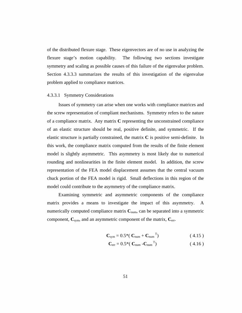
51

of the distributed flexure stage. These eigenvectors are of no use in analyzing the

flexure stage’s motion capability. The following two sections investigate

symmetry and scaling as possible causes of this failure of the eigenvalue problem.

Section 4.3.3.3 summarizes the results of this investigation of the eigenvalue

problem applied to compliance matrices.

4.3.3.1 Symmetry Considerations

Issues of symmetry can arise when one works with compliance matrices and

the screw representation of compliant mechanisms. Symmetry refers to the nature

of a compliance matrix. Any matrix C representing the unconstrained compliance

of an elastic structure should be real, positive definite, and symmetric. If the

elastic structure is partially constrained, the matrix C is positive semi-definite. In

this work, the compliance matrix computed from the results of the finite element

model is slightly asymmetric. This asymmetry is most likely due to numerical

rounding and nonlinearities in the finite element model. In addition, the screw

representation of the FEA model displacement assumes that the central vacuum

chuck portion of the FEA model is rigid. Small deflections in this region of the

model could contribute to the asymmetry of the compliance matrix.

Examining symmetric and asymmetric components of the compliance

matrix provides a means to investigate the impact of this asymmetry. A

numerically computed compliance matrix Cnum, can be separated into a symmetric

component, Csym, and an asymmetric component of the matrix, Cerr.

Csym = 0.5*( Cnum + Cnum T) ( 4.15 )

Cerr = 0.5*( Cnum -Cnum T) ( 4.16 )

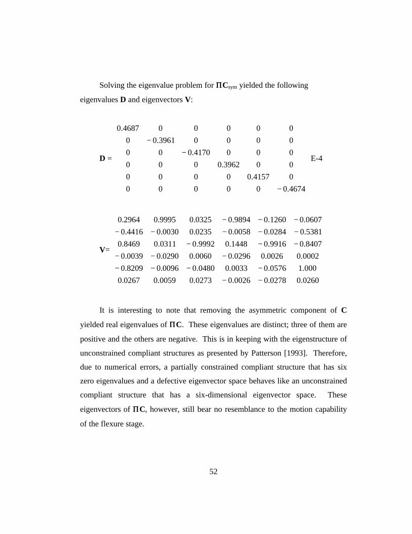
52

Solving the eigenvalue problem for ΠΠCsym yielded the following

eigenvalues D and eigenvectors V:

D =

−

−−

4674.000000

04157.00000

003962.0000

0004170.000

00003961.00

000004687.0

E-4

V=

−−−−−−

−−−−−−−−−−−−−−

0260.00278.00026.00273.00059.00267.0

000.10576.00033.00480.00096.08209.0

0002.00026.00296.00060.00290.00039.0

8407.09916.01448.09992.00311.08469.0

5381.00284.00058.00235.00030.04416.0

0607.01260.09894.00325.09995.02964.0

It is interesting to note that removing the asymmetric component of C

yielded real eigenvalues of ΠΠC. These eigenvalues are distinct; three of them are

positive and the others are negative. This is in keeping with the eigenstructure of

unconstrained compliant structures as presented by Patterson [1993]. Therefore,

due to numerical errors, a partially constrained compliant structure that has six

zero eigenvalues and a defective eigenvector space behaves like an unconstrained

compliant structure that has a six-dimensional eigenvector space. These

eigenvectors of ΠΠC, however, still bear no resemblance to the motion capability

of the flexure stage.

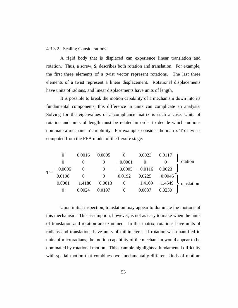
53

4.3.3.2 Scaling Considerations

A rigid body that is displaced can experience linear translation and

rotation. Thus, a screw, $, describes both rotation and translation. For example,

the first three elements of a twist vector represent rotations. The last three

elements of a twist represent a linear displacement. Rotational displacements

have units of radians, and linear displacements have units of length.

It is possible to break the motion capability of a mechanism down into its

fundamental components, this difference in units can complicate an analysis.

Solving for the eigenvalues of a compliance matrix is such a case. Units of

rotation and units of length must be related in order to decide which motions

dominate a mechanism’s mobility. For example, consider the matrix T of twists

computed from the FEA model of the flexure stage:

T=

−−−−−

−−−−

0230.00037.000197.00024.00

4549.14169.100013.04180.10001.0

0046.00225.00192.0000198.0

0023.00116.00005.0000005.0

000001.0000

0117.00023.000005.00016.00

Upon initial inspection, translation may appear to dominate the motions of

this mechanism. This assumption, however, is not as easy to make when the units

of translation and rotation are examined. In this matrix, rotations have units of

radians and translations have units of millimeters. If rotation was quantified in

units of microradians, the motion capability of the mechanism would appear to be

dominated by rotational motion. This example highlights a fundamental difficulty

with spatial motion that combines two fundamentally different kinds of motion:

rotation

translation

54

translation and rotation. The scale of these motions must be considered in order

to determine the dominant motions of a body.

4.3.3.3 Summary of the Eigenvalue Problem

While the eigenstructure of a compliant mechanism is a good indicator of

its kinematic and load bearing characteristics, its use in comparing the specific

stages of Figures 3.7 and 3.11 is limited. The repeated zero eigenvalues and a

defective eigenvector space of the ideal stage lead to poorly conditioned

numerical approximations of the flexure stage. A robust numerical scheme is

therefore required for comparing the ideal and flexure stages. The following

section presents such an approach based on strain energy.

4.3.4 The Use of Strain Energy as a Metric

The difficulty of characterizing the behavior of numerically computed non-

ideal compliant structures using eigenvalues and eigenvectors illustrates the need

for an alternative metric to compare the motion capabilities of compliant spatial

mechanisms. The physical quantity of strain energy may be used as such a

metric. The amount of work done by a force is the product of a force and the

distance through which it acts:

W = F d ( 4.17 )

where

W = work done by a force F (units of energy)

F = applied force (units of force)

d = the distance through which the force acts (units of length)

The work done by a wrench acting on a compliant structure may be

calculated in a similar manner:

W = Tf̂ ΠΠ t̂ = E ( 4.18 )

55

where

W = work done by wrench (units of energy)

f̂ = wrench applied to structure (units of force, torque)

t̂ = twist representation of structure’s deflection (units of length, rotation)

E = strain energy stored in deformed compliant structure (units of energy)

The amount of strain energy stored in a compliant structure is equal to the

amount of work an applied wrench performs. In fact, a structure’s compliance

determines how much strain energy the structure can store in a given

configuration. As a wrench deforms an elastic structure, strain energy is stored in

compliant members of the structure. Wrenches of the same magnitude applied

along stiff portions of an elastic structure will cause little deformation and store

little strain energy in the system.

This relationship can be exploited to find wrenches that are “near-

reciprocal” to a mechanism. Given an applied wrench and resulting twist, one can

calculate the strain energy stored in a compliant structure via Equation 4.18.

Wrenches that generate little or no strain energy in the structure are assumed to be

near-reciprocal wrenches.

Wrenches and twists computed via the FEA model of the flexure stage

confirm this analysis. Table 4.1 lists strain energies calculated from wrenches and

twists taken from the FEA model of the flexure stage.

56

Table 4.1 Strain energy in distributed flexure stage

Strain Energy Applied wrench

1.3185 15 lb. force along x axis

94.6136 15 lb. force along y axis

1.3125 15 lb. force along z axis

116.1306 10 in-lb. torque about x axis

1.4617 10 in-lb. torque about z axis

119.0054 10 in-lb. torque about y axis

Small strain energies indicate that wrenches consisting of forces along the x

and y axes and moments about the z axis are reciprocal to the distributed flexure

stage. These three wrenches span the space of wrenches reciprocal to the stage.

Wrenches with large strain energies are not reciprocal to the stage. These results

confirm that the distributed flexure stage exhibits the motions that are desired in a

wafer orientation stage. The flexure stage allows rotations about x and y and

translation in z. At the same time, it has low translation in x and y and rotation

about z.

4.4 Summary

This chapter examined the ideal stage presented in Section 3.2 and the

distributed flexure stage presented in Section 3.5. These two stages were

compared to determine the suitability of the distributed flexure stage for use as a

wafer orientation stage for imprint lithography. The eigenvalue problem provides

a good tool for examining the motion capability of the ideal stage. The

distributed flexure stage, however, could only be analyzed using the strain energy

metric previously discussed. Both stages exhibit motion characteristics

appropriate for use in an imprint lithography orientation stage.

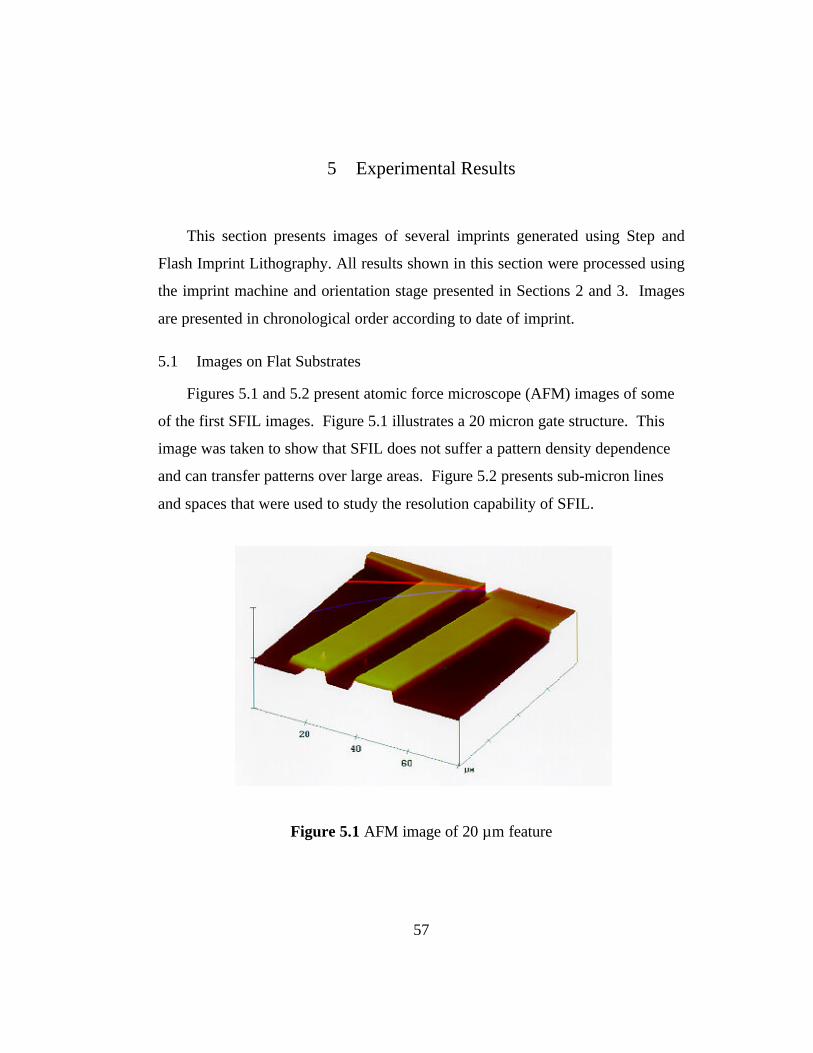
57

5 Experimental Results

This section presents images of several imprints generated using Step and

Flash Imprint Lithography. All results shown in this section were processed using

the imprint machine and orientation stage presented in Sections 2 and 3. Images

are presented in chronological order according to date of imprint.

5.1 Images on Flat Substrates

Figures 5.1 and 5.2 present atomic force microscope (AFM) images of some

of the first SFIL images. Figure 5.1 illustrates a 20 micron gate structure. This

image was taken to show that SFIL does not suffer a pattern density dependence

and can transfer patterns over large areas. Figure 5.2 presents sub-micron lines

and spaces that were used to study the resolution capability of SFIL.

Figure 5.1 AFM image of 20 µm feature

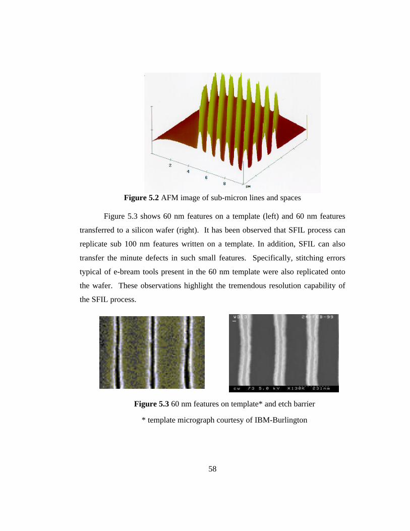
58

Figure 5.2 AFM image of sub-micron lines and spaces

Figure 5.3 shows 60 nm features on a template (left) and 60 nm features

transferred to a silicon wafer (right). It has been observed that SFIL process can

replicate sub 100 nm features written on a template. In addition, SFIL can also

transfer the minute defects in such small features. Specifically, stitching errors

typical of e-bream tools present in the 60 nm template were also replicated onto

the wafer. These observations highlight the tremendous resolution capability of

the SFIL process.

Figure 5.3 60 nm features on template* and etch barrier

* template micrograph courtesy of IBM-Burlington

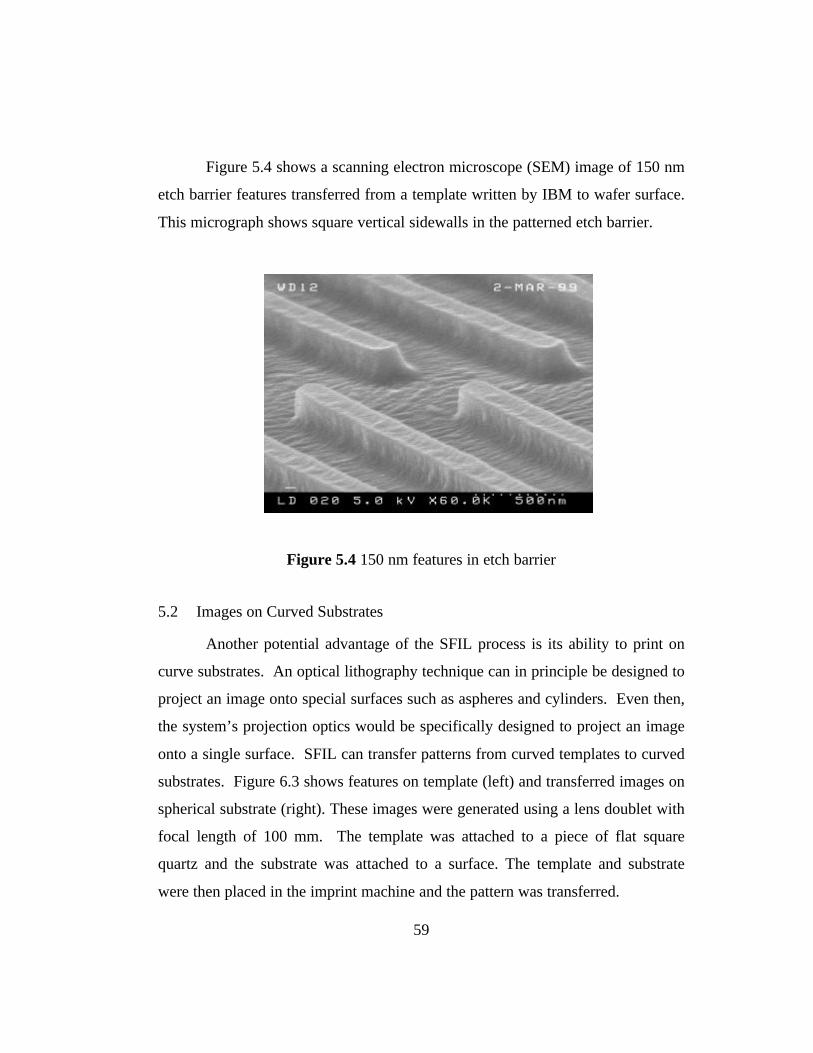
59

Figure 5.4 shows a scanning electron microscope (SEM) image of 150 nm

etch barrier features transferred from a template written by IBM to wafer surface.

This micrograph shows square vertical sidewalls in the patterned etch barrier.

Figure 5.4 150 nm features in etch barrier

5.2 Images on Curved Substrates

Another potential advantage of the SFIL process is its ability to print on

curve substrates. An optical lithography technique can in principle be designed to

project an image onto special surfaces such as aspheres and cylinders. Even then,

the system’s projection optics would be specifically designed to project an image

onto a single surface. SFIL can transfer patterns from curved templates to curved

substrates. Figure 6.3 shows features on template (left) and transferred images on

spherical substrate (right). These images were generated using a lens doublet with

focal length of 100 mm. The template was attached to a piece of flat square

quartz and the substrate was attached to a surface. The template and substrate

were then placed in the imprint machine and the pattern was transferred.

60

Figure 5.5 Optical micrographs of images on curved template and substrate

Figure 5.6 presents SEM (left) and AFM (right) images of a patterned etch

barrier on a curved substrate. A dotted circle in Figure 5.5 indicates the location

of these images on the substrate.

Figure 5.6 SEM and AFM images of patterned spherical substrate

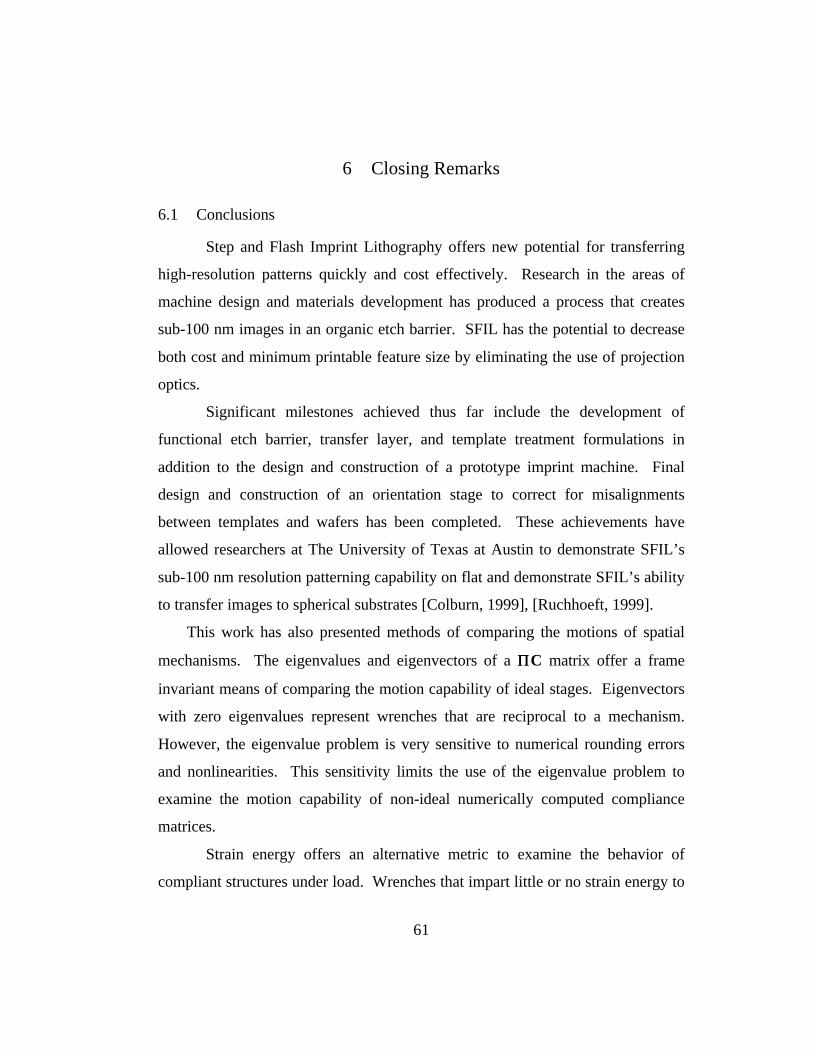
61

6 Closing Remarks

6.1 Conclusions

Step and Flash Imprint Lithography offers new potential for transferring

high-resolution patterns quickly and cost effectively. Research in the areas of

machine design and materials development has produced a process that creates

sub-100 nm images in an organic etch barrier. SFIL has the potential to decrease

both cost and minimum printable feature size by eliminating the use of projection

optics.

Significant milestones achieved thus far include the development of

functional etch barrier, transfer layer, and template treatment formulations in

addition to the design and construction of a prototype imprint machine. Final

design and construction of an orientation stage to correct for misalignments

between templates and wafers has been completed. These achievements have

allowed researchers at The University of Texas at Austin to demonstrate SFIL’s

sub-100 nm resolution patterning capability on flat and demonstrate SFIL’s ability

to transfer images to spherical substrates [Colburn, 1999], [Ruchhoeft, 1999].

This work has also presented methods of comparing the motions of spatial

mechanisms. The eigenvalues and eigenvectors of a ΠΠC matrix offer a frame

invariant means of comparing the motion capability of ideal stages. Eigenvectors

with zero eigenvalues represent wrenches that are reciprocal to a mechanism.

However, the eigenvalue problem is very sensitive to numerical rounding errors

and nonlinearities. This sensitivity limits the use of the eigenvalue problem to

examine the motion capability of non-ideal numerically computed compliance

matrices.

Strain energy offers an alternative metric to examine the behavior of

compliant structures under load. Wrenches that impart little or no strain energy to

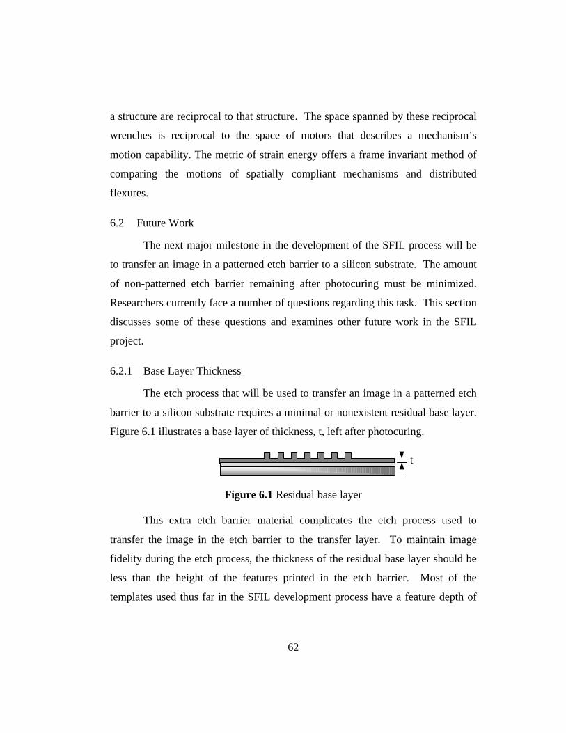
62

a structure are reciprocal to that structure. The space spanned by these reciprocal

wrenches is reciprocal to the space of motors that describes a mechanism’s

motion capability. The metric of strain energy offers a frame invariant method of

comparing the motions of spatially compliant mechanisms and distributed

flexures.

6.2 Future Work

The next major milestone in the development of the SFIL process will be

to transfer an image in a patterned etch barrier to a silicon substrate. The amount

of non-patterned etch barrier remaining after photocuring must be minimized.

Researchers currently face a number of questions regarding this task. This section

discusses some of these questions and examines other future work in the SFIL

project.

6.2.1 Base Layer Thickness

The etch process that will be used to transfer an image in a patterned etch

barrier to a silicon substrate requires a minimal or nonexistent residual base layer.

Figure 6.1 illustrates a base layer of thickness, t, left after photocuring.

Figure 6.1 Residual base layer

This extra etch barrier material complicates the etch process used to

transfer the image in the etch barrier to the transfer layer. To maintain image

fidelity during the etch process, the thickness of the residual base layer should be

less than the height of the features printed in the etch barrier. Most of the

templates used thus far in the SFIL development process have a feature depth of

t

63

100 to 200 nm. Currently, researches are attempting to reduce the thickness of the

base layer to less than 100 nm.

This problem can be attacked from two directions: dispensing just enough

fluid to wet the surfaces and removing any excess liquid. The manner in which

the liquid etch barrier is dispensed seems to affect the amount of residual etch

barrier left behind. Simply placing a drop of the etch barrier on the wafer and

pressing the template onto the wafer leaves base layers 10 microns thick and

thicker. Filling the gap between the template and wafer has produced base layer

thicknesses on the order of one micron. Spin coating the etch barrier on the wafer

before printing may further minimize residual base layer thicknesses, but this

method is difficult to implement. It is difficult to keep a spin coated wafer clean

when transporting it from the spinner to the imprint machine. One should also

note that etch barriers are solutions of compounds of differing weights. Spin

coating may push heavier elements towards the edge of the wafer and leave a non

uniform etch barrier on the wafer.

The amount of liquid etch barrier dispensed may also be related to the

thickness of the base layer. One should dispense just enough liquid to wet the

template-wafer interface and fill all of the voids of the template. Any excess

liquid not expelled to the edge of the template before photocuring will contribute

to the residual base layer.

Alternative methods for dispensing the etch barrier could include wetting

the template. The template could be spin-coated with etch barrier and then

pressed onto the wafer. Alternatively, a thin later of etch barrier could be painted

onto the template before it is mated to a silicon wafer. Creative thinking in this

area may sidestep some critical technical issues that could delay SFIL

development

64

6.2.2 Scientific Investigation

The problem of minimizing excess etch barrier material leads one to

consider a number of fundamental questions about the interface between the

template and the wafer. What mechanisms dominate the filling process as the

liquid etch barrier wets the surfaces of the template and wafer? What is the most

effective means of wetting these surfaces? What forces dominate the behavior of

the etch barrier as the template and wafer are pressed together? At the

macroscopic level, shear forces in the liquid will expel it to the edges of the

template, but what happens as the thickness of the etch barrier film approaches

zero? Answers to these questions and others will lead to greater understanding of

the SFIL process.

6.2.3 Sensing

Sensing issues will play a key role in the investigation of the interface of

the template and wafer. Currently, the SFIL project posses no means of

measuring the distance between the template and wafer as they approach one

another. Answering many of the questions posed in the previous section will

require a sensing system to clarify the mechanics of the template-wafer interface

during various steps of the SFIL process.

Capacitive sensors have been considered for measuring this gap distance,

but optical systems would be easier to implement. Broad band interference

sensors such as those to measure film thicknesses (DRM type tools) are well

understood, but these systems can only measure gaps down to a few hundred

nanometers. A sensing scheme that produces an interferogram of the gap between

the template and the wafer would give the user more information than a single

point sensing system. An interferogram could indicate particle contamination or

waviness in the silicon wafer, but such a system is more complex than a single

65

point system. Researchers on the SFIL project are currently investigating these

systems.

Sensing systems are needed for two purposes: investigating the behavior

of the template-wafer interface and characterizing alignment during the actual

imprint process. One could construct a test bed solely for the purpose of

investigating the template-wafer interface. Such a testbed would probably

incorporate an interferogram type sensor or a point sensor mounted on a precision

x-y table. This arrangement would allow one to investigate the gap thickness

between two substrates that have been pressed together. Data from this testbed

may indicate that a set of point sensors is sufficient for alignment during the

printing process. Again, an understanding of the behavior of the template, wafer,

and etch barrier will be key to future progress in the development of the SFIL

process.

6.2.4 Active and Passive Stages

The issue of active versus passive stages will likely have to be addressed

before a practical step and repeat tool can be completed. Passive stages are

simpler than active stages and offer very high repeatability for lower cost and

complexity. Their simplicity makes them an elegant solution to orientation and

alignment needs of the SFIL process if they work. However, an active orientation

stage may be required to fully implement SFIL. If one wants to control the

spacing of the template and wafer without making contact, an active stage is

required. Furthermore, overlay will be difficult at best if an SFIL machine does

not incorporate an active stage. It may be possible to predict the behavior of a

passive stage, but one cannot alter the behavior of an passive stage during the

imprint process, in other words, a passive stage cannot incorporate error

correction and feedback into an operating scheme.

66

6.2.5 Overlay

To eventually see integrated circuits manufactured with SFIL, overlay

must at least be considered during the development process. The decision to

avoid high forces and high temperatures during the SFIL process implicitly

acknowledges the importance of this subject. To construct a multi-layer

semiconductor device, succesive circuit layers have to be aligned or overlayed.

The SFIL project need not develop an overlay scheme to align numerous

images, but it should consider the needs of an overlay scheme. For example, one

may have to incorporate an active stage in an eventual SFIL stepper to achieve the

desired overlay accuracy. To make the greatest possible contribution to SFIL

development, mechanical stage design work should consider the needs of

potential overlay systems.

6.2.6 Template Loading and Deformation

The method of holding the template during the imprint process may

require further investigation. Simply clamping the template in a few places may

significantly deform the template and distort and image written on the template.

By avoiding high temperatures, SFIL avoids thermal expansion and contraction of

the template. Deformation due to fixturing forces also merits consideration. This

deformation may be enough to disrupt the operation of a circuit manufactured

with SFIL. Overlay could also be affected by these distortions.

67

Appendix A

MATLAB Code to Compute Compliance Kinematic Model

The following file computes the compliance matrix, eigenvalues, and

eigenscrews for the ideal kinematic model.

clear all% threeD.m% this routine finds the compliance matrix for a three legged parallellinkage% it then computes the eigenvalues and eigenvectors of the compliancematrix

% Eigenscrew analysis of 3 DOF kinematic model of orientation stagel = 1; % length of side of stage triangle

% Define spring compliancesd = zeros(6,6);d(1,1) = 0; % denotes reciprocal wrenchd(2,2) = 0; % denotes reciprocal wrenchd(3,3) = 0; % denotes reciprocal wrenchd(4,4) = 1; % compliance of spring 1d(5,5) = 1; % compliance of spring 2d(6,6) = 1; % compliance of spring 3

% Define p and w vectors for each screw

p1 = [1/2;-sqrt(3)/6;0]*l;p1r = p1;p2 = [0;1/sqrt(3);0]*l;p2r = p2;p3 = [-1/2;-sqrt(3)/6;0]*l;p3r = p3;w1 = [1/2;sqrt(3)/2;0];w2 = [-1;0;0];w3 = [1/2;-sqrt(3)/2;0];w1r = [0;0;1];w2r = w1r;w3r = w1r;

% Construct screws from p's and w's

pw1 = cross(p1,w1);pw2 = cross(p2,w2);pw3 = cross(p3,w3);pw1r = cross(p1r,w1r);pw2r = cross(p2r,w2r);pw3r = cross(p3r,w3r);

68

s1 = cat(1,w1,pw1);s2 = cat(1,w2,pw2);s3 = cat(1,w3,pw3);s1r = cat(1,w1r,pw1r);s2r = cat(1,w2r,pw2r);s3r = cat(1,w3r,pw3r);

J = cat(2,s1,s2,s3,s1r,s2r,s3r)

% Compute compliance matrixC = ((inv(J')))*d*inv(J);piop = [zeros(3),eye(3);eye(3),zeros(3)];pC = piop*C;[V,D] = eig(C);[pV,pD] = eig(pC);

format shortCdisp('Pi times C:');pCdisp('Eigenvalues of Pi times C:');pDdisp('Eigenvectors of Pi times C:');pV

69

Appendix B

MATLAB Code to Compute Compliance Matrix of Distributed Flexure Stage

This code computes a compliance matrix describing the displacement of

the distributed orientation stage for a given applied wrench. Proc.m reads data

node displacement data generated from an IDEAS finite element model. The data

is formatted and passed to twist.m. Twist.m calculates a twist vector given two

sets of points as input. The output from twist.m is then used to compute a

compliance matrix.

% proc.m% this file reads node displacement data files and computes atwist vector% for every displacement field

% clear all values from memory and set display format to longclear all;format long e;

% read initial node locationsnodeloc = dlmread('nodeloc.txt',' ');x0 = nodeloc(:,2:4);

% read displaced node locationsdata = dlmread('data.txt',' ');

% parse node locations into 6 separate matricesx1 = data(1:22,2:4);x2 = data(23:44,2:4);x3 = data(45:66,2:4);x4 = data(67:88,2:4);x5 = data(89:110,2:4);x6 = data(111:132,2:4);

% select three points in each displacement fields0(1,:) = x0(1,:);s0(2,:) = x0(5,:);s0(3,:) = x0(13,:);s0 = s0'-[0,0,0;30,30,30;0,0,0];

s1(1,:) = x1(1,:);

70

s1(2,:) = x1(5,:);s1(3,:) = x1(13,:);s1 = s1' + s0;

s2(1,:) = x2(1,:);s2(2,:) = x2(5,:);s2(3,:) = x2(13,:);s2 = s2' + s0;

s3(1,:) = x3(1,:);s3(2,:) = x3(5,:);s3(3,:) = x3(13,:);s3 = s3' + s0;

s4(1,:) = x4(1,:);s4(2,:) = x4(5,:);s4(3,:) = x4(13,:);s4 = s4' + s0;

s5(1,:) = x5(1,:);s5(2,:) = x5(5,:);s5(3,:) = x5(13,:);s5 = s5' + s0;

s6(1,:) = x6(1,:);s6(2,:) = x6(5,:);s6(3,:) = x6(13,:);s6 = s6' + s0;

% Compute twist vectors for all six displacement fieldstw1 = twist(s0,s1);tw2 = twist(s0,s2);tw3 = twist(s0,s3);tw4 = twist(s0,s4);tw5 = twist(s0,s5);tw6 = twist(s0,s6);

% assemble twist matrixtwt = zeros(6,6);tw = zeros(6,6);

twt(:,1) = tw1;twt(:,2) = tw2;twt(:,3) = tw3;twt(:,4) = tw4;twt(:,5) = tw5;twt(:,6) = tw6;

tw(:,1) = twt(:,1);

71

tw(:,2) = twt(:,2);tw(:,3) = twt(:,3);

% Subtract first three twists from last three twists if flag = 1flag = 0;

if flag == 0 tw(:,4) = twt(:,4); tw(:,5) = twt(:,5); tw(:,6) = twt(:,6);end

if flag == 1 tw(:,4) = twt(:,4)-twt(:,1); tw(:,5) = twt(:,5)-twt(:,2); tw(:,6) = twt(:,6)-twt(:,2);end

%tw(4:6,4:6) = 0

% filter twist matrix by zeroing any translation smaller than 10microns% and zeroing any rotation smaller than 0.1 milliradian

flag = 0;if flag == 1 for j = 1:6 % loop through all twists for i = 1:3 % loop through rotations if tw(i,j) <= 0.0001 tw(i,j) = 0; end end for i = 4:6 % loop through translations if tw(i,j) <= 0.001 tw(i,j) = 0; end end endend

% Read load node locationsloadread = dlmread('loadloc.txt',' ');loadloc1 = loadread(1,2:4);loadloc2 = loadread(1,2:4);loadloc3 = loadread(1,2:4);loadloc4 = loadread(2,2:4);loadloc5 = loadread(3,2:4);

72

loadloc6 = loadread(4,2:4);

% compute rho vectors for wrenchesrho1 = (loadloc1-loadloc1)';rho2 = (loadloc2-loadloc1)';rho3 = (loadloc3-loadloc1)';rho4 = (loadloc4-loadloc1)';rho5 = (loadloc5-loadloc1)';rho6 = (loadloc6-loadloc1)';

% compute w vectors for wrenchesmagn = 15*4.44822; %newtonsw1 = [1;0;0];w2 = [0;-1;0];w3 = [0;0;1];w4 = [1;0;0];w5 = [0;-1;0];w6 = [0;-1;0];

% compute wrencheswr1 = zeros(6,1);wr2 = zeros(6,1);wr3 = zeros(6,1);wr4 = zeros(6,1);wr5 = zeros(6,1);wr6 = zeros(6,1);

wr1(1:3) = w1*magn;wr2(1:3) = w2*magn;wr3(1:3) = w3*magn;wr4(1:3) = w4*magn;wr5(1:3) = w5*magn;wr6(1:3) = w6*magn;

wr1(4:6) = cross(rho1,w1)*magn;wr2(4:6) = cross(rho2,w2)*magn;wr3(4:6) = cross(rho3,w3)*magn;wr4(4:6) = cross(rho4,w4)*magn;wr5(4:6) = cross(rho5,w5)*magn;wr6(4:6) = cross(rho6,w6)*magn;

% Assemble wrench matrixwr = zeros(6,6);wrt = zeros(6,6);

wrt(:,1) = wr1;wrt(:,2) = wr2;wrt(:,3) = wr3;wrt(:,4) = wr4;

73

wrt(:,5) = wr5;wrt(:,6) = wr6;

wr(:,1) = wrt(:,1);wr(:,2) = wrt(:,2);wr(:,3) = wrt(:,3);

% Subtract first three wrenches from last three wrenches if flag= 1flag = 0;

if flag == 0 wr(:,4) = wrt(:,4); wr(:,5) = wrt(:,5); wr(:,6) = wrt(:,6);end

if flag ==1 wr(:,4) = wrt(:,4)-wrt(:,1); wr(:,5) = wrt(:,5)-wrt(:,2); wr(:,6) = wrt(:,6)-wrt(:,2);end

% Compute pi operator matrixp = [zeros(3),eye(3);eye(3),zeros(3)];

% Compute CpC_num = tw*inv(wr);C_num = p*pC_num;

% scale values of translations and rotations and compute C_numagainflag = 1;if flag ==1 testCforce = [C_num(1,1),C_num(2,2),C_num(3,3)]; testCmoment = [C_num(4,4),C_num(5,5),C_num(6,6)]; a = max(testCforce) b = max(testCmoment) s = a/b

twscaled = tw twscaled(1:3,:) = twscaled(1:3,:)*s; twscaled

pC_num = twscaled*inv(wr); C_num = p*pC_num;end

% Make C symmetric if flag = 1

74

flag = 1;

if flag ==1 C = 0.5*(C_num + C_num'); C_noise = 0.5*(C_num - C_num');else C = C_numend

pC = p*C;

% Compute eigenvalues of C and pi*C[V,D] = eig(C);[pV,pD] = eig(pC);

% normalize eigenvectors if flag = 1;flag = 1;if flag ==1 pV(1:6,1) = pV(1:6,1)/norm(pV(1:3,1)); pV(1:6,2) = pV(1:6,2)/norm(pV(1:3,2)); pV(1:6,3) = pV(1:6,3)/norm(pV(1:3,3)); pV(1:6,4) = pV(1:6,4)/norm(pV(1:3,4)); pV(1:6,5) = pV(1:6,5)/norm(pV(1:3,5)); pV(1:6,6) = pV(1:6,6)/norm(pV(1:3,6));end

% normalize length components of eigenvectorsflag = 1;if flag ==1 temp = max(pV(4:6,:)); temp = max(temp) pV(4:6,:) = pV(4:6,:)/temp;end

format short% Calculate work done my each wrenche1 = wr(:,1)'*p*tw(:,1)e2 = wr(:,2)'*p*tw(:,2)e3 = wr(:,3)'*p*tw(:,3)e4 = wr(:,4)'*p*tw(:,4)e5 = wr(:,5)'*p*tw(:,5)e6 = wr(:,6)'*p*tw(:,6)

% Display symmetric C and noise component of CC%C_noise

% Display twists and wrenchestw

75

wr

% Display C and its eigenvalues and eigenscrewsCDV

% Display Pi*C and its eigenvalues and eigenscrewspCpDpV

The following function, twist.m, computes the screw representation of the

displacement of a rigid body. The function reads initial and final positions of

three points on the rigid body and outputs a twist.

function [twistout] = twist(si,sf)

% given three initial points and three displaced points, this file% computes a corresponding twist vector

p1i = si(:,1);p2i = si(:,2);p3i = si(:,3);

p1f = sf(:,1);p2f = sf(:,2);p3f = sf(:,3);

% Compute rotation matricespinit = zeros(3,3);pfin = zeros(3,3);

pinit(:,1) = p2i-p1i;pinit(:,1) = pinit(:,1)/norm(pinit(:,1));

pinit(:,2) = cross(pinit(:,1),p3i-p1i);pinit(:,2) = pinit(:,2)/norm(pinit(:,2));

pinit(:,3) = cross(pinit(:,1),pinit(:,2));pinit(:,3) = pinit(:,3)/norm(pinit(:,3));

pfin(:,1) = p2f - p1f;pfin(:,1) = pfin(:,1)/norm(pfin(:,1));

76

pfin(:,2) = cross(pfin(:,1),p3f - p1f);pfin(:,2) = pfin(:,2)/norm(pfin(:,2));

pfin(:,3) = cross(pfin(:,1),pfin(:,2));pfin(:,3) = pfin(:,3)/norm(pfin(:,3));

Qi = eye(3);Qf = pinit*inv(pfin);

% Compute displacement vectorsqi = p1i;qf = p1f;

% 1. compute gg = qf - qi;

% 2. compute M and mM = Qi*(Qf'); % <------ Remember thism = qf-M*qi;

% 3. compute cthetactheta = (M(1,1)+M(2,2)+M(3,3)-1)/2;theta = acos(ctheta);

% 4. form ll = zeros(3,1);l(1) = M(3,2)-M(2,3);l(2) = M(1,3)-M(3,1);l(3) = M(2,1)-M(1,2);

% 5. compute ltmltm = l'*m;

% 6. determine sign(ctheta), compute sin(theta)theta = theta*sign(ltm);stheta = sin(theta);

% 7. form ww = l/(2*stheta);

% 8. compute dd = ltm/(2*stheta);

% 9. compute rhoI = eye(3);rho = (I-M')*m/2/(1-ctheta);

% 10. compute hh = d/theta;

77

% check to see if ctheta = 1 or ctheta = -1%ctheta%range = 0.05;%if (1-range)<ctheta,(1+range);% disp('cos(theta) = 1 verify results');%end%if (-1-range)<ctheta,(-1+range);% disp('cos(theta) = -1 verify results');%end

% assemble twist vectortwist = zeros(6,1);twist(1:3) = w;twist(4:6) = cross(rho,w) + w*h;twistout = twist*theta;

78

References

Badami, V. G., Smith, S. T., and Patterson, S.R., “A metrological three-axis

translator and its application for constant force profilometry,” Proceedings

of the Eleventh Annual Meeting of the American Society for Precision

Engineering, 1996, pp. 391-395.

Choi, B. J., 1998, “Kinematic Design, Motion/Force Coordination, and

Performance Analysis of Force Controlled Wheeled Vehicles”, Ph.D.

Dissertation, Mechanical Engineering, The University of Texas at Austin.

Colburn, M., Johnson, S., Stewart, M., Damle, S., Choi, B.J., Bailey, T.,

Sreenivasan, S.V., Ekerdt, J., and Willson, C.G., "Step and Flash Imprint

Lithography: An alternative approach to high resolution patterning."

SPIE's 24th Intl. Symp. Microlithography: Emerging Lithographic

Technologies III. March 14-19, 1999 Santa Clara, CA.

Gere, J. and Timoshenko, S., Mechanics of Materials, Third Edition, PWS

Publishing Company, Boston, 1990.

Haisma, J.; Verheijen, M.; van der Huevel, K.;van den Berg, J.; “Template-

assisted nanolithography: A process for reliable pattern replication”. J.

Vac. Sci. Technol. B 14(6) (Nov/Dec 1996)

Hunt, K. H., 1990, "Kinematic Geometry of Mechanisms”, Oxford: Clarendon

Press.

P. Ruchhoeft, M. Colburn, H. Nounu, S. Damle, S. Johnson, M. Stewart, T.

Bailey, B. Choi, S.V. Sreenivasan, J. Ekerdt, J. C. Wolfe and C. G.

Willson, “Patterning Curved Surfaces: Template Generation by Ion

Proximity Lithography and Relief Transfer by Step and Flash Imprint

Lithography”, J. Vac. Sci. Technol., B, Oct/Nov, 1999.

79

Patterson, T., and Lipkin, H., “Structure of Robot Compliance,” ASME Journal of

Mechanical Design, Vol. 115, 1993, pp.576-580.

Smith, Stuart, and Chetwynd, D.G., “Foundations of Ultraprecision Mechanism

Design,” Gordon and Breach Science Publishers, Philadelphia, 1992.

Strang, Gilbert. “Linear Algebra and Its Applications,” Harcourt Brace

Jovanovich, Publishers, San Diego, 1988.

Thompson, Larry F., Willson, C. Grant, and Bowden, Murrae J., Introduction to

Microlithography, 2nd ed., American Chemical Society, Washington, DC,

1994.

Waldron, K. J., Course Notes for ME 851 Kinematic Geometry of Mechanisms,

The Ohio State University, 1993.

Waldron, K. J., Raghavan, M. and Roth, B., “Kinematics of a Hybrid Series-

Parallel Manipulation System,” ASME Journal of Dynamic Systems,

Measurement, and Control, Vol. 111, 1989, pp. 211-221.

80

Vita

Stephen Christopher Johnson was born in Tulsa, Oklahoma on December

8, 1974, the son of Carolyn Ann Johnson and James Massey Johnson. After

completing his work at James E. Taylor High School in Katy, Texas, in 1993, he

entered The University of Texas at Austin in Austin, Texas. He received the

degree of Bachelor of Science from The University of Texas at Austin in August,

1997. In September, 1997, he entered The Graduate School at The University of

Texas at Austin.

Permanent Address: 910 Kentbury Ct.

Katy, Texas 77450

This thesis was typed by the author.

Documents

Copyright Stephen Christopher Johnson