Embed Size (px)
Citation preview

Copyright is owned by the Author of the thesis. Permission is given for a copy to be downloaded by an individual for the purpose of research and private study only. The thesis may not be reproduced elsewhere without the permission of the Author.

Symmetric Parallel
Class Expression Learning
TRAN, Cong An
School of Engineering and Advanced Technology
Massey University
New Zealand
A thesis submitted in partial fulfilment of the requirements for the degree of
Doctor of Philosophy
in
Computer Science
June, 2013

ii

For my grandparents, my parents, my wife and my son
iii

iv

Acknowledgements
I would like to take this opportunity to thank my supervisors, Prof. Hans
W. Guesgen, Prof. Jens Dietrich and Prof. Stephen Marsland for their guid-
ance and support. I am thankful that I could benefit from their combined
research experience. Prof. Hans W. Guesgen introduced me the world of
Ambient Intelligent with its humanistic ideas of helping the elderly to have
a better life. Prof. Jens Dietrich attracted me to his colourful world of Soft-
ware Engineering. His endless source of ideas impressed me that this is the
world of the active and creative people. Prof. Stephen Marsland, a ‘diverse’
professor with the excellent background in mathematics and computer sci-
ence, encouraged me into his mysterious world of Machine Learning.
I also want to thank Jens Lehmann, the research group leader of Machine
Learning and Ontology Engineering (MOLE) Group at the University of
Leipzig, as well as the author of the DL-Learner framework, for his kind-
ness to grant me permission to access his DL-Learner framework repository
as well as for his valuable advice to evaluate learners. I also highly appre-
ciate Prof. Adrian Paschke, Director of RuleML Inc., for his advice on my
research direction.
I would like to thank the Ministry of Education and Training of Vietnam
for awarding me the scholarship for my study. Thanks also go to the School
of Engineering and Advanced Technology (SEAT) for the financial support
that has enabled me to attend international conferences, which not only
improved my research but also enriched my life.
Thanks to all members of Massey University Smart Home (MUSE) research
group for their valuable discussions and feedbacks on my research. I also
v

want to thank Michele Wagner for her administrative support throughout
my degree.
This thesis would not be possible without the warm and support of my
Palmy-based family, Mr. Vo The Truyen and his family, Mr. Nguyen Buu
Huan and Mr. Nguyen Van Long, who give me a home away from home.
In particular, my special thanks go to Mr. Truyen’s for treating me as
their little brother and Mr. Huan for checking and giving me many helpful
advices on my writing. I could not have asked for more warm and kind
friends as them.
Finally, I would like to give all my deepest gratitude and respect to my fam-
ily. To my grandparents and my parents for their continuous love, support
and patience. To my parents-in-law for taking good care of my son in more
than four years, which released me from family concerns to concentrate on
my research. To my sister and brother for being with my parents during my
study. To my beloved wife, Nguyen Thu Huong, and my son, Tran Cong
Huan. It is my fortune to have them in my life. They are always by my
side to share all the laughers and tears.
vi

Abstract
The growth of both size and complexity of learning problems in description logic
applications, such as the Semantic Web, requires fast and scalable description logic
learning algorithms. This thesis proposes such algorithms using several related ap-
proaches and compares them with existing algorithms. Particular measures used for
comparison include computation time and accuracy on a range of learning problems of
different sizes and complexities.
The first step is to use parallelisation inspired by the map-reduce framework. The
top-down learning approach, coupled with an implicit divide-and-conquer strategy, also
facilitates the discovery of solutions for a certain class of complex learning problems. A
reduction step aggregates the partial solutions and also provides additional flexibility
to customise learnt results.
A symmetric class expression learning algorithm produces separate definitions of
positive (true) examples and negative (false) examples (which can be computed in
parallel). By treating these two sets of definitions ‘symmetrically’, it is sometimes
possible to reduce the size of the search space significantly. The use of negative example
denotions enhances learning problems with exceptions, where the negative examples
(‘exceptions’) follow a few relatively simple patterns.
In general, correctness (true positives) and completeness (true negatives) of a learn-
ing algorithm are traded off against each other because these two criteria are normally
conflicting. Particular learning algorithms have an inherent bias towards either cor-
rectness or completeness. The use of negative definitions enables an approach (called
fortification in this thesis) to improve predictive correctness by applying an appropriate
level of over-specialisation to the prediction model, while avoiding over-fitting.
The experiments presented in the thesis show that these algorithms have the po-
tential to improve both the computation time and predictive accuracy of description
logic learning when compared to existing algorithms.
vii

viii
Contents
Acknowledgement v
Abstract vii
List of Figures xiii
List of Tables xv
1 Introduction 1
1.1 Introduction . . . . . . . . . . . . . . . . . . . . . . . . . . . . . . . . . . 1
1.2 Motivation . . . . . . . . . . . . . . . . . . . . . . . . . . . . . . . . . . 3
1.3 Scope of Study . . . . . . . . . . . . . . . . . . . . . . . . . . . . . . . . 8
1.4 Aims and Objectives . . . . . . . . . . . . . . . . . . . . . . . . . . . . . 8
1.5 Thesis Overview . . . . . . . . . . . . . . . . . . . . . . . . . . . . . . . 10
2 Preliminaries and Related Work 13
2.1 Description Logics and Web Ontology Language . . . . . . . . . . . . . 13
2.1.1 Description logic languages . . . . . . . . . . . . . . . . . . . . . 13
2.1.2 Description logic knowledge bases . . . . . . . . . . . . . . . . . 17
2.1.3 The Web Ontology Language (OWL) . . . . . . . . . . . . . . . 23
2.2 Description Logic and OWL Learning . . . . . . . . . . . . . . . . . . . 26
2.2.1 Description logic learning problem . . . . . . . . . . . . . . . . . 26
2.2.2 Basic approaches in DL learning . . . . . . . . . . . . . . . . . . 29
2.3 Related Work . . . . . . . . . . . . . . . . . . . . . . . . . . . . . . . . . 32
2.3.1 Description logic learning . . . . . . . . . . . . . . . . . . . . . . 32
ix

CONTENTS
2.3.2 Parallel description logic learning . . . . . . . . . . . . . . . . . . 34
2.3.3 Numerical data learning in description logics . . . . . . . . . . . 35
2.3.4 Class Expression Learner for Ontology Engineering (CELOE) . . 36
3 Evaluation Methodology 39
3.1 Introduction . . . . . . . . . . . . . . . . . . . . . . . . . . . . . . . . . . 39
3.2 Evaluation Metrics . . . . . . . . . . . . . . . . . . . . . . . . . . . . . . 40
3.2.1 Accuracy . . . . . . . . . . . . . . . . . . . . . . . . . . . . . . . 40
3.2.2 Learning time . . . . . . . . . . . . . . . . . . . . . . . . . . . . . 41
3.2.3 Definition length . . . . . . . . . . . . . . . . . . . . . . . . . . . 42
3.2.4 Search space size . . . . . . . . . . . . . . . . . . . . . . . . . . . 42
3.3 Experimental Design . . . . . . . . . . . . . . . . . . . . . . . . . . . . . 42
3.3.1 Experimental framework . . . . . . . . . . . . . . . . . . . . . . . 42
3.3.2 Comparison algorithms . . . . . . . . . . . . . . . . . . . . . . . 48
3.3.3 Evaluation Datasets . . . . . . . . . . . . . . . . . . . . . . . . . 50
3.4 Implementation and Running the Code . . . . . . . . . . . . . . . . . . 58
4 Adaptive Numerical Data Segmentation 61
4.1 Introduction . . . . . . . . . . . . . . . . . . . . . . . . . . . . . . . . . . 61
4.2 Motivation . . . . . . . . . . . . . . . . . . . . . . . . . . . . . . . . . . 62
4.3 Description of Our Method . . . . . . . . . . . . . . . . . . . . . . . . . 65
4.4 The Algorithms . . . . . . . . . . . . . . . . . . . . . . . . . . . . . . . . 67
4.5 Evaluation Results . . . . . . . . . . . . . . . . . . . . . . . . . . . . . . 68
4.5.1 Segmentation result . . . . . . . . . . . . . . . . . . . . . . . . . 70
4.5.2 Experimental results on the accuracy . . . . . . . . . . . . . . . . 71
4.6 Conclusion . . . . . . . . . . . . . . . . . . . . . . . . . . . . . . . . . . 75
5 Parallel Class Expression Learning 77
5.1 Parallelisation for Class Expression Learning . . . . . . . . . . . . . . . 77
5.2 Description of Our Method . . . . . . . . . . . . . . . . . . . . . . . . . 79
5.3 The Algorithms . . . . . . . . . . . . . . . . . . . . . . . . . . . . . . . . 83
5.4 Evaluation Result . . . . . . . . . . . . . . . . . . . . . . . . . . . . . . . 88
x
CONTENTS
5.4.1 Experiment 1 - Comparison between ParCEL and CELOE . . . 89
5.4.2 Experiment 2 - Effect of parallelisation on learning speed . . . . 96
5.4.3 Experiment 3 - Definition reduction strategy . . . . . . . . . . . 98
5.5 Conclusion . . . . . . . . . . . . . . . . . . . . . . . . . . . . . . . . . . 100
6 Symmetric Class Expression Learning 103
6.1 Exceptions in Learning . . . . . . . . . . . . . . . . . . . . . . . . . . . . 103
6.2 Symmetric Class Expression Learning . . . . . . . . . . . . . . . . . . . 106
6.2.1 Overview of our method . . . . . . . . . . . . . . . . . . . . . . . 106
6.2.2 Description of our method . . . . . . . . . . . . . . . . . . . . . . 108
6.2.3 The algorithm . . . . . . . . . . . . . . . . . . . . . . . . . . . . 111
6.2.4 Counter-partial definitions combination strategies . . . . . . . . . 116
6.3 Evaluation . . . . . . . . . . . . . . . . . . . . . . . . . . . . . . . . . . . 118
6.3.1 Experiment 1 - Combination strategies comparison . . . . . . . . 119
6.3.2 Experiment 2 - Search tree size comparison . . . . . . . . . . . . 122
6.3.3 Experiment 3 - Predictive accuracy and learning time . . . . . . 124
6.3.4 Experiment 4 - The learnt definitions . . . . . . . . . . . . . . . 128
6.4 Conclusion . . . . . . . . . . . . . . . . . . . . . . . . . . . . . . . . . . 132
7 Improving Predictive Correctness by Fortification 135
7.1 Problem Description . . . . . . . . . . . . . . . . . . . . . . . . . . . . . 135
7.2 Fortification Candidates Generation . . . . . . . . . . . . . . . . . . . . 140
7.3 Fortification Strategy . . . . . . . . . . . . . . . . . . . . . . . . . . . . . 143
7.3.1 Fortification candidates scoring . . . . . . . . . . . . . . . . . . . 143
7.3.1.1 Training coverage scoring . . . . . . . . . . . . . . . . . 144
7.3.1.2 Fortification concept similarity scoring . . . . . . . . . . 145
7.3.1.3 Fortification validation scoring . . . . . . . . . . . . . . 157
7.3.1.4 Random score . . . . . . . . . . . . . . . . . . . . . . . 160
7.3.2 Fortification cut-off point computation . . . . . . . . . . . . . . . 160
7.4 Evaluation . . . . . . . . . . . . . . . . . . . . . . . . . . . . . . . . . . . 161
7.4.1 Fortification evaluation methodology . . . . . . . . . . . . . . . . 161
7.4.2 Experimental results . . . . . . . . . . . . . . . . . . . . . . . . . 162
xi

CONTENTS
7.5 Conclusion . . . . . . . . . . . . . . . . . . . . . . . . . . . . . . . . . . 176
8 Conclusions and Future Work 181
8.1 Discussion and Contributions of the Thesis . . . . . . . . . . . . . . . . 181
8.2 Threats to Validity of the Results . . . . . . . . . . . . . . . . . . . . . . 184
8.2.1 Threats to internal validity . . . . . . . . . . . . . . . . . . . . . 184
8.2.2 Threats to external validity . . . . . . . . . . . . . . . . . . . . . 186
8.3 Future Work . . . . . . . . . . . . . . . . . . . . . . . . . . . . . . . . . 187
A Accessing the Implementation 191
A.1 Software Structure . . . . . . . . . . . . . . . . . . . . . . . . . . . . . . 191
A.1.1 DL-Learner architecture . . . . . . . . . . . . . . . . . . . . . . . 191
A.1.2 Our algorithms packages . . . . . . . . . . . . . . . . . . . . . . . 192
A.2 Checking Out and Compiling Code . . . . . . . . . . . . . . . . . . . . . 193
A.2.1 Checking out the project . . . . . . . . . . . . . . . . . . . . . . 194
A.2.2 Compiling code . . . . . . . . . . . . . . . . . . . . . . . . . . . . 195
B Reproducing the Experimental Results 197
B.1 System Requirements . . . . . . . . . . . . . . . . . . . . . . . . . . . . 197
B.2 Running the Experiments . . . . . . . . . . . . . . . . . . . . . . . . . . 198
B.2.1 Syntax . . . . . . . . . . . . . . . . . . . . . . . . . . . . . . . . . 198
B.2.2 Learning configuration file naming conventions . . . . . . . . . . 199
B.3 Learning Configuration . . . . . . . . . . . . . . . . . . . . . . . . . . . . 199
B.4 Test Cases . . . . . . . . . . . . . . . . . . . . . . . . . . . . . . . . . . . 202
C List of Publications 211
Glossary 213
References 217
xii
List of Figures
1.1 A typical search tree produced by a top-down learning approach for the
Tweety problem. . . . . . . . . . . . . . . . . . . . . . . . . . . . . . . . 6
2.1 An example of the top-down approach in DL learning . . . . . . . . . . 31
2.2 An example of the bottom-up approach in DL learning . . . . . . . . . . 32
3.1 Data partition for a 10-fold cross-validation . . . . . . . . . . . . . . . . 44
3.2 An example of the inconsistency in parallel learning . . . . . . . . . . . 45
3.3 Termination of learning algorithms . . . . . . . . . . . . . . . . . . . . . 48
3.4 The MUSE dataset ontology visualised in Protege . . . . . . . . . . . . 55
3.5 RDF graph of an activity in the MUSE dataset . . . . . . . . . . . . . . 56
3.6 The concept hierarchy of the MUBus dataset visualised in Protege . . . 57
4.1 Specialisation of numeric datatype properties. . . . . . . . . . . . . . . . 63
4.2 Segmentation of numeric datatype properties . . . . . . . . . . . . . . . 64
4.3 Inappropriate segmentation of the data property values prevents the spe-
cialisation of an overly general expression . . . . . . . . . . . . . . . . . 64
4.4 A relation graph between examples and numeric values . . . . . . . . . . 66
4.5 Segmentation of data property values . . . . . . . . . . . . . . . . . . . . 67
4.6 Segmentation of the data property values in Figure 4.3 . . . . . . . . . . 67
5.1 The specialisation using a downward refinement operator . . . . . . . . 81
5.2 Parallel exploration of the search tree using two workers . . . . . . . . . 83
5.3 Reducer-Worker interaction. . . . . . . . . . . . . . . . . . . . . . . . . . 84
xiii
LIST OF FIGURES
5.4 Accuracy against learning time of CELOE and ParCEL on the Carcino-
Genesis dataset using different number of workers. . . . . . . . . . . . . 96
5.5 Accuracy against learning time of CELOE and ParCEL on the UCA1
dataset using different number of workers. . . . . . . . . . . . . . . . . . 97
5.6 Speed-up efficiency of ParCEL on the UCA1 dataset. . . . . . . . . . . . 98
6.1 Exception patterns in learning . . . . . . . . . . . . . . . . . . . . . . . 105
6.2 Different approaches to learning the definition for the extended Tweety
learning problem. . . . . . . . . . . . . . . . . . . . . . . . . . . . . . . . 107
6.3 The top-down learning step aims to find both partial definitions and
counter-partial definitions . . . . . . . . . . . . . . . . . . . . . . . . . . 111
6.4 Top-down learning in SPaCEL with multiple workers. . . . . . . . . . . 112
7.1 The creation of a prediction model for a learning problem . . . . . . . . 137
7.2 A prediction scenario of the prediction model in Figure 7.1 . . . . . . . 138
7.3 Decrease of predictive accuracy caused by inappropriate fortification. . . 139
7.4 Fortification candidates learning . . . . . . . . . . . . . . . . . . . . . . 141
7.5 Family concepts hierarchy. . . . . . . . . . . . . . . . . . . . . . . . . . . 150
A.1 DL-Learner architecture . . . . . . . . . . . . . . . . . . . . . . . . . . . 193
B.1 Check required softwares in the system including JDK, Subversion and
Maven. . . . . . . . . . . . . . . . . . . . . . . . . . . . . . . . . . . . . . 206
B.2 Install required softwares for compilation the project: JDK, Subversion
and Maven . . . . . . . . . . . . . . . . . . . . . . . . . . . . . . . . . . 206
B.3 Check out the project from the repository . . . . . . . . . . . . . . . . . 207
B.4 Compile the DL-Leaner and ParCEL core components project. . . . . . 207
B.5 Compile the interface project. . . . . . . . . . . . . . . . . . . . . . . . . 207
B.6 Compile the ParCEL CLI project. . . . . . . . . . . . . . . . . . . . . . 207
B.7 Command line to learn the Forte-Uncle dataset using CELOE . . . . . . 208
B.8 Command line to learn the Forte-Uncle dataset using ParCEL . . . . . . 208
B.9 Command line to learn the Forte-Uncle dataset using SPaCEL . . . . . 209
xiv
List of Tables
2.1 Basic concept constructors in description logics . . . . . . . . . . . . . . 15
2.2 Letters used to name description logic languages. . . . . . . . . . . . . . 16
2.3 The semantics of basic concept constructors in description logics. . . . . 18
2.4 DLs notations and OWL notations . . . . . . . . . . . . . . . . . . . . . 24
2.5 OWL constructors and the corresponding constructors in DLs . . . . . . 25
3.1 Size and complexity of the evaluation datasets . . . . . . . . . . . . . . 51
3.2 Properties of the evaluation datasets . . . . . . . . . . . . . . . . . . . . 52
4.1 Reduction of numeric data properties values resulting from the adaptive
segmentation strategy. . . . . . . . . . . . . . . . . . . . . . . . . . . . . 70
4.2 Training and predictive accuracies of CELOE on the ILDP dataset using
for the two segmentation strategies. . . . . . . . . . . . . . . . . . . . . . 72
4.3 Training and predictive accuracies of ParCEL on the ILDP dataset using
for the two segmentation strategies. . . . . . . . . . . . . . . . . . . . . . 73
4.4 Predictive accuracy of CELOE and ParCEL on the UCA1 dataset using
for the two segmentation strategies. . . . . . . . . . . . . . . . . . . . . . 74
5.1 ParCEL and CELOE experimental results. . . . . . . . . . . . . . . . . 90
5.2 Balanced accuracy of CELOE and ParCEL on unbalanced datasets. . . 94
5.3 ParCEL and CELOE experimental results with one worker. . . . . . . . 95
5.4 Speed-up of ParCEL on the UCA1 dataset . . . . . . . . . . . . . . . . . 98
5.5 Definition length comparison between three reduction strategies . . . . . 99
6.1 Basic description learning algorithms and their usage of examples. . . . 108
xv
LIST OF TABLES
6.2 SPaCEL experimental result – Combination strategies . . . . . . . . . . 119
6.3 SPaCEL experimental results – The search tree size . . . . . . . . . . . 123
6.4 SPaCEL experimental result – Learning time and predictive accuracy . 124
6.5 Balanced predictive accuracy of unbalanced datasets . . . . . . . . . . . 127
6.6 SPaCEL experimental result – Definition length of the learning problem 128
7.1 Fortification experimental result with CELOE . . . . . . . . . . . . . . . 166
7.2 Fortification experimental result on ParCEL . . . . . . . . . . . . . . . . 170
7.3 Fortification experimental result with SPaCEL . . . . . . . . . . . . . . 173
7.4 Experimental results for new cut-off points . . . . . . . . . . . . . . . . 178
B.1 Common components in DL-Learner framework and their parameters . 200
B.2 Actions and expected result of the test case. . . . . . . . . . . . . . . . . 204
xvi
Chapter 1
Introduction
In this chapter, we first provide the research background of the thesis, partic-
ularly the description logic learning problem, and identify the problems to be
addressed. Next, we describe the motivations and the aims and objectives of
this thesis. Finally, we present an overview of the thesis.
1.1 Introduction
Description logic learning has its roots in Inductive Logic Programming (ILP), a sym-
bolic approach in machine learning that aims to learn general rules from specific facts
[76, 77, 102, 104]. Given a background knowledge and a set of observed facts repre-
sented in the form of logic programs [51, 86, 99], ILP aims to learn a set of rules that
describe the given facts. Therefore, it can be used to derive new knowledge (the learnt
rules) from the current knowledge and observed facts:
knowledge baseobserved facts−−−−−−−−−→ (learnt) rules.
In description logic learning, description logics (DLs) are employed to represent
the knowledge bases and observed facts. DLs are a family of formal knowledge rep-
resentation languages that emerged from earlier research on semantic networks and
frame-based systems [4, 98, 109, 125]. Given a knowledge base and two sets of in-
stances (called positive and negative example sets) represented in description logics,
1
1. Introduction
description logic learning aims to find a description such that all positive (true) exam-
ples are instances of the learnt description1 and none of the negative (false) examples
is an instance of the learnt description (see Chapter 2 for basic concepts in description
logics). The elements of the positive and negative example sets are called positive and
negative examples respectively. The learnt description corresponds to the learnt rule in
inductive logic programming and it is called the definition of the positive examples. It
can be considered as the new knowledge derived from the observations (i.e. from posi-
tive and negative examples). Example 1.1 illustrates a simple description logic learning
problem.
Example 1.1 (A simple example of description logic learning). Consider a
knowledge base that contains four classes: Person, Male, Female and Uncle; three
properties: married, hasSibling and hasChild; and some instances of these classes
that relate to the description of the uncle relationship. A general description logic learn-
ing algorithm can produce description(s) that describe the uncle concept, for example
(written in Manchester OWL syntax [62]):
Male AND (hasSibling SOME (hasChild SOME Person) OR
(married SOME hasSibling SOME hasChild SOME Person))
�
The biggest benefits of symbolic over sub-symbolic approaches in machine learn-
ing are the interpretability and the rich hierarchical structure and semantics of the
knowledge base. The interpretability of symbolic approaches is represented by two
aspects. First, knowledge represented in logic-based languages is generally easier for
humans to analyse and understand than the forms of knowledge representation used in
sub-symbolic approaches as it is relatively close to human knowledge representation.
Second, many logic reasoners, particularly web ontology language reasoners such as
RacerPro [55] and Pellet [107], provide justifications of inferences [71]. Justifications,
also called explanations or traces, are a (minimal) set of rules sufficient to produce an
inference. They can be considered as explanations of an inference and can be used
to justify a decision made by a decision support system. For example, the inference
1It is also said that the description covers the instances.
2

1. Introduction
“John is a father” can be supported by an explanation, such as, ‘(because) John
is man AND he has a child”. Therefore, justifications can help to increase the trust
(in the inferences produced by systems) of systems that use this approach. This is an
essential requirement for some types of application that require a high level of trust
in the decisions of the system such as expert systems for human disease diagnosis, or
decision support systems for elderly care.
Description logics are the underlying logic language of the Web Ontology Language
(OWL), which was endorsed as a standard ontology language for the Semantic Web
[14] by the World Wide Web Consortium (W3C)2 in 2004 [96]. With the advent of
semantic technologies, particularly the Semantic Web, OWL has become a prominent
paradigm for knowledge representation and reasoning.
Currently, the semantic web is growing steadily – it has developed from more than
10 million semantic web pages in 2010 to approximately 230.6 million in 2011 [24]. It
contains knowledge from various areas such as biomedicine, science, social networks,
and general (upper) ontologies [54, 94, 105, 119]. Coupled with the development of
web ontology language and semantic web applications, the demand for techniques for
automated schema acquisition is increasing [16, 83, 89, 90, 112, 143]. Consequently,
many induction techniques for description logics have been proposed [32, 45, 80, 85,
114, 115] to meet this demand. They are used in various applications in domains
including biology, medicine, cognitive systems and software engineering [35, 60, 125].
1.2 Motivation
Description logic learning problems are increasing in both size (the number of concepts
and instances in the knowledge base) and complexity (the number of concepts and
roles in the learnt description). This raises the need for faster learning algorithms
to process the tasks faster by using system resources such as CPU and memory more
effectively. More importantly, when the applications get bigger and more complex,
scalability becomes a critical requirement. This property indicates the ability of the
learning algorithm to deal with large and complex learning problems.
2http://www.w3.org/Consortium/
3
1. Introduction
As an example, a decision support system in a bank often has only limited resources
to perform maintenance works such as learning credit card fraud detection patterns from
a day’s data to update its information system, e.g. within 1 hour from 1am everyday.
This is a strict requirement regardless of how many transactions have been performed
that day. As another example, consider an abnormal behaviour detection for elderly
care in smart homes, in which a learning algorithm is called to update the definition
of abnormal behaviour when new patterns in the inhabitant’s behaviour emerge. The
normal/abnormal behaviour patterns may become more complicated over time. To
ensure that the detection system does not miss any abnormal behaviours caused by
long learning time, a learning algorithm is often required to run within a given duration
regardless of the complexity of the learning problem. Therefore, the learning algorithms
are required to deal with the various complexity levels of the learning problems so that
they are usable in real-word applications.
Learning in description logics is essentially a search problem: it searches for a right
description3 in the search space that consists of potential descriptions constructed
from the vocabulary of the language. The potential descriptions in the search space are
usually generated dynamically by an operator such as downward/upward refinement or
the Most Specific Concepts (MSC) operator (see Section 2.2). Therefore, the speed of
a description learning approach depends upon the number of computations (searches)
per second and the number of computations per answer, i.e. the time to find the right
answer. On the other hand, the scalability can be influenced by the learning strategy,
i.e. how to construct the solution.
A popular technique for speeding up programs is parallelisation, which takes the
advantage of multi-core processors and multi-processor systems. Multiple searches can
run concurrently on multiple cores to increase the number of computations per second.
While this technique has been applied to inductive logic programming to speed up the
learning algorithms, it has not yet been used in description logic learning. In this thesis,
we propose an approach to parallel description logic learning that uses the advantages
of parallelisation to speed up the learning algorithm.
In addition, we also employ the implicit divide and conquer learning strategy to help
3Complete and correct description with respect to the sets of examples (c.f. Section 2.2)
4

1. Introduction
our learning approach to handle complex learning problems more effectively. The basic
idea behind this strategy is to allow the learning algorithm to learn the definitions
for subsets of instances in the positive example set, i.e. partial solutions, and then
combine them to construct a final solution. The subsets of instances are not explicitly
divided, but they are implicitly defined depending on the definitions found by the
learning algorithm. Intuitively, finding partial solutions is likely to be easier than
finding a complete one. A similar learning strategy was reported in the literature
(see Section 2.3). However, the combination of definitions in the approach in the
literature simply creates the disjunction of all definitions and thus the solution is likely
to contain redundancies. We address this problem by proposing a reduction before the
combination step to select the best definitions for the combination.
The second method for speeding up the learning algorithm is to reduce the number
of computations required to find a solution. In a learning approach based on search,
the number of computations for finding the solution is basically affected by two factors:
i) the search heuristics, and ii) the effectiveness of using the descriptions in the search
space. The search heuristic controls the selection of the descriptions in the search space
for further solution exploration. This factor can be adjusted according to particular
learning problem.
The strategy for using descriptions in the search space suggests a more general
approach to reduce the number of computations needed to find a solution. Existing de-
scription logic learning approaches reported in the literature (see Section 2.3) generate
and search for descriptions that cover all positive and no negative examples. Descrip-
tions that cover only negative examples are removed from the search space as they
are said to be useless for learning the solution. A problem with this approach is that
sometimes descriptions in the search space are not used effectively.
To illustrate this point, consider a classical example used in logic programming,
Tweety, which can be used to learn the definition of flying birds. This problem comes
with a knowledge base that contains a hierarchical structure of concepts, a set of pos-
itive examples that contains instances of flying birds, and a set of negative examples
containing instances of birds and other objects that cannot fly (such as penguins).
Then, the expected definition for positive examples is Bird � ¬Penguin. A typical
5

1. Introduction
Figure 1.1: A typical search tree produced by a top-down learning approach for theTweety problem.
TOP
Bird
TOP concept in DLs
definition
Bird TOP Bird
Penguin
Penguin
Bird Bird Bird Penguin
Bird Penguin
TOP TOP . . .
search space (tree) produced by a top-down learning approach for this problem is given
in Figure 1.1. Popular description logic learning algorithms will ignore the description
Penguin in the search tree as it does not cover any positive examples. However, this
simple definition of the negative examples can be combined with another simple de-
scription Bird to construct the solution that is Bird AND not Penguin to describe the
flying birds. This thesis addresses this problem by proposing a ‘symmetric’ description
logic leaning approach that uses definitions of both positive and negative examples in
learning the solution. This approach uses the descriptions in the search tree more effec-
tively, which can help to reduce the necessary search space size for learning a problem.
As a consequence, this approach can improve the learning speed.
In description logic learning, the top-down approach, also called specialisation, is
commonly used as it can facilitate the rich hierarchical structure of knowledge bases to
construct the search space. Definitions learnt by this approach are likely to be shorter
and more concise than those of other approaches [82]. For this reason, they are often
more general than the learnt definitions of other approaches (see Section 2.2.2 for a
discussion of the generality of a definition). Consequently, the learnt definitions of this
approach favour completeness (the true positive) over correctness (the true negative)
of the prediction. This bias may fit certain kinds of application. However, there are
also applications that prefer correctness to completeness.
As an example, consider a surveillance system that learns the normal behaviour
pattern of the elderly and use the patterns, coupled with the ‘negation as failure’
inference rule, for detecting abnormal behaviours. The learnt pattern is complete if it
6
1. Introduction
can cover all normal behaviours and correct if it does not cover any abnormal behaviour.
In such a system, correctness of the learnt definitions is favoured over completeness as
misclassifying abnormal behaviours as normal ones may threaten the person’s safety.
The above scenarios, together with the symmetric approach in description logic
learning, motivate us to propose a method that can provide a trade-off between com-
pleteness and correctness of the prediction for description logic learning algorithms.
The basic idea of this approach is to fortify the learnt definitions by including redun-
dant specialisations to improve the predictive correctness. The redundant specialisation
is performed by using a set of negative example definitions. In addition, to prevent the
over-specialisation of the learnt definition, the redundant specialisation is controlled by
a fortification strategy. This strategy aims to estimate the level of specialisation that
should be applied to the learnt definitions.
We also propose a method for numerical data refinement that will be the basis for
algorithms to learn numerical data. This is motivated by the fact that the existing
description logic learning algorithms mainly focus upon learning the concepts without
having appropriate attention for learning numeric data. In fact, learning symbolic
concepts is the ultimate purpose of the symbolic learning approach and thus it is
reasonable for the existing learning algorithms to pay attention to this aspect. However,
there is also the fact that there are certain circumstances in which the data needs to
be represented numerically.
To learn the numeric datatype properties, we need to identify a set of values used for
refinement and then define the refinement operator on the set. Most existing description
logic learning approaches attempt to use a fixed-size segmentation method to identify
the set of values for refinement. Given a set of all asserted values of a numeric datatype
property, the fixed-size segmentation approach divides the values into a fixed number of
segments. Then, values on the boundaries of the segments are used for the refinement
operator. However, this method may produce redundant values or miss necessary values
for refinement. Therefore, we propose a novel approach for the dynamic segmentation
of numeric datatype properties values based on a relation graph. Our approach can
eliminate the redundancy and the insufficiency of the refinement values.
7
1. Introduction
1.3 Scope of Study
The work of this thesis is mainly related to description logic learning, particularly the
web ontology language. Specific limitations include:
• Symbolic approach: the learning technique used in our thesis is based on induction
and the knowledge is represented using description logics, particularly the Web
Ontology Language (OWL).
• Supervised learning: the learning is based on labelled datasets.
• Positive and negative learning setting: this thesis is restricted to the positive and
negative examples learning setting where the training dataset must contain both
positive and negative examples. In supervised learning, this learning setting is
more general than the other one: the positive examples only learning setting.
• Numeric data learning: our approach supports the integer and real datatype, and
two restrictions: maximal (≤) and minimal value (≥).
1.4 Aims and Objectives
This thesis is about improving the speed and scalability of description logic learning,
and providing a flexible trade-off between completeness and correctness of the pre-
dictions in description logic learning. First, our method for segmentation of numeric
datatype provides a better strategy in learning numeric data for description logic learn-
ing algorithms. Then, two approaches to speed up and scale up the description logic
learning are proposed to help the learning algorithm to deal with various types and
complexity levels of learning problems. Finally, the fortification method supports a
flexible and configurable balance between correctness and completeness to match the
requirements of particular applications. The detailed objectives of this thesis are listed
below.
1. The first objective is to provide a method to segment the values of datatype
properties. It is expected to be able to compute a set of values used for refinement
of the datatype properties in the learning problem such that:
8

1. Introduction
• none of the values needed to distinguish between positive and negative ex-
amples are missed, and
• redundant values that are unnecessary for distinguishing between positive
and negative examples can be eliminated.
2. The second objective is to provide a parallel description learning algorithm that
is able to:
• find a definition for a set of positive examples given sets of positive and
negative examples and a knowledge base,
• utilise parallel computing to find the sub-solutions in parallel to increase the
learning speed and ability to handle complex learning problems, and
• provide basic reduction strategies to aggregate sub-solutions into a final so-
lution.
3. The third objective is to develop a description logic learning algorithm that can
learn from labelled data symmetrically and is able to:
• learn definitions for both positive and negative examples,
• provide combination strategies for combining the descriptions that are nether
the definitions of positive examples nor negative examples with the defini-
tions of negative examples to create definitions for positive examples, and
• provide basic reduction strategies to aggregate definitions of positive exam-
ples into a final solution.
4. The final objective of this thesis is to provide a method for fortifying the predictive
correctness in description logic learning that is able to:
• learn the negative examples definitions (called fortifying definitions) using a
given description logic learning algorithm, and
• select the best fortifying definitions for fortification such that the predictive
correctness can be increased without decreasing the predictive accuracy.
9

1. Introduction
All the above objectives are evaluated using the cross-validation method on a set
of datasets that vary in size, complexity (i.e. length of the target definition), noise
(i.e. with and without noise) and field of application (e.g. biology, smart homes and
transportation). The experimental results are compared with other description logic
learning algorithms to assess the efficacy of our approaches.
1.5 Thesis Overview
This thesis is organised into 8 chapters, including this chapter, and 2 appendices.
The contributions of this thesis are described in chapters 4-7. Other chapters provide
supplementary background knowledge, description of the evaluation method as well as
discussion on the results and findings of the thesis. An overview of the chapters is given
below.
Chapter 2 (Preliminaries and Related Works) covers the background knowledge
related to description logic learning, which helps with understanding the remaining
chapters in the thesis. It briefly introduces the history of description logic learning
and then some elementary concepts in this research area. Then, two basic approaches
of description logic learning, the top-down and bottom-up approaches, are described
along with a list of applications of description logic learning. This chapter ends with a
literature review of this research.
Chapter 3 (Evaluation Methodology) describes the methodology used for the
evaluation, which plays an important role in this research. This chapter first introduces
some classic datasets used in the evaluation. These datasets have been widely used in
the evaluations of other machine learning research. In addition, one novel smart home
datasets and another dataset extracted from a bus service schedule are also presented.
Next, details of the evaluation methodology are described including the cross-
validation methodology and a statistical significance test. Some details of the computer
system and learning configuration used for the evaluations are also discussed. Finally,
this chapter introduces the learning algorithms that are used as the comparators to
evaluate the algorithms proposed in this thesis.
10

1. Introduction
Chapter 4 (An Approach to Numeric Data Property Values Segmentation)
proposes a method for computing the values used for refinement of numeric datatype
properties. This chapter first describes current approaches to refinement of numeric
datatype properties in description logic learning and identifies their limitations. Then,
it describes an approach for dynamic segmentation of numeric datatype property val-
ues to address the problems of the existing approaches. Finally, an implementation
is introduced and experimental results are shown to demonstrate the efficacy of the
approach.
Chapter 5 (An Approach to Parallel Class Expression Learning) introduces a
parallel description logic learning approach that combines the top-down method with
an aggregation method to speed up the learning algorithm. It uses an explicit divide
and conquer strategy to find the sub-solutions. This helps the learning algorithm to
handle complex learning problems more easily. In addition, this approach also requires
an aggregation to build the final solution. We introduce a reduction step before the
aggregation to reduce the redundancy in the final solution. Some reduction strategies
are proposed corresponding to certain properties of the learnt definitions such as the
definition length, or the number of sub-solutions.
Chapter 6 (Symmetric Class Expression Learning) proposes a method that can
reduce the search space by using sets of positive and negative examples symmetrically.
This method learns definitions for both positive and negative examples simultaneously.
Definitions of negative examples are then used to construct the definitions of positive
examples. This approach uses the descriptions in the search space effectively and thus
it can help to increase the learning speed. It is also shown that this approach is suitable
for learning problems that contain exceptions.
Chapter 7 (Improving Predictive Correctness by Fortification) presents a
method for improving the predictive correctness in description logic learning. It first
describes an idea for learning the fortifying definitions given a description logic learning
algorithm. Then, some strategies for selecting the best candidates for the fortification
are described. We also introduce a method for estimating the cut-off point for the
11

1. Introduction
fortification. The experimental results are compared with the original learning results
(i.e., without fortification) to assess the impact of this technique.
Chapter 8 (Conclusions and Future Works) concludes the results and the findings
of this thesis, and outlines the prospects for future work.
Appendix A (Accessing the Implementation) introduces the implementation of
the methods proposed in this thesis. This chapter first introduces briefly the DL-
Learner, an open source machine learning framework our implementations rely on.
Then, the structure of the implementation is described. Finally, instructions to check-
out and compile the implementation from its repository are provided.
Appendix B (Reproducing the Experimental Results) provides instructions for
reproducing the experimental results reported in this thesis.
12
Chapter 2
Preliminaries and Related Work
This chapter provides the background of this thesis, description logic (DL)
learning, and its related work. DLs and the web ontology languages, the rep-
resentation languages used in the proposed algorithms, are first introduced.
Then, DL learning is described including basic concepts, notations and ap-
proaches. This chapter ends with a summary of recent work in DL learning.
2.1 Description Logics and Web Ontology Language
This thesis is about the inductive learning for description logics, particularly the web
ontology language. Therefore, this section first provides an overview of these languages.
Description logics (DLs) is a family of knowledge representation formalisms that
emerged from earlier research on semantic networks and frame-based systems [3, 98,
109]. The earliest work on description logics is called ‘structured inheritance networks’
by Brachman [21]. They are essentially fragments of first order logic [118] with less
expressive power. However, most variants of description logics are decidable, which is
one of the desirable properties of a knowledge representation language [3].
2.1.1 Description logic languages
A description logic knowledge base is constructed based on a vocabulary, which consists
of concept names (atomic concept), role names and objects (individuals), and a set of
13
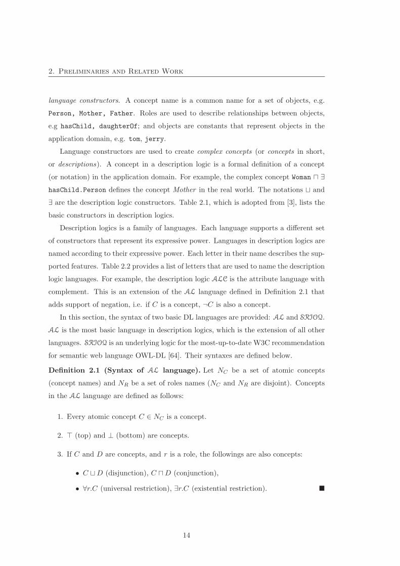
2. Preliminaries and Related Work
language constructors. A concept name is a common name for a set of objects, e.g.
Person, Mother, Father. Roles are used to describe relationships between objects,
e.g hasChild, daughterOf; and objects are constants that represent objects in the
application domain, e.g. tom, jerry.
Language constructors are used to create complex concepts (or concepts in short,
or descriptions). A concept in a description logic is a formal definition of a concept
(or notation) in the application domain. For example, the complex concept Woman � ∃hasChild.Person defines the concept Mother in the real world. The notations � and
∃ are the description logic constructors. Table 2.1, which is adopted from [3], lists the
basic constructors in description logics.
Description logics is a family of languages. Each language supports a different set
of constructors that represent its expressive power. Languages in description logics are
named according to their expressive power. Each letter in their name describes the sup-
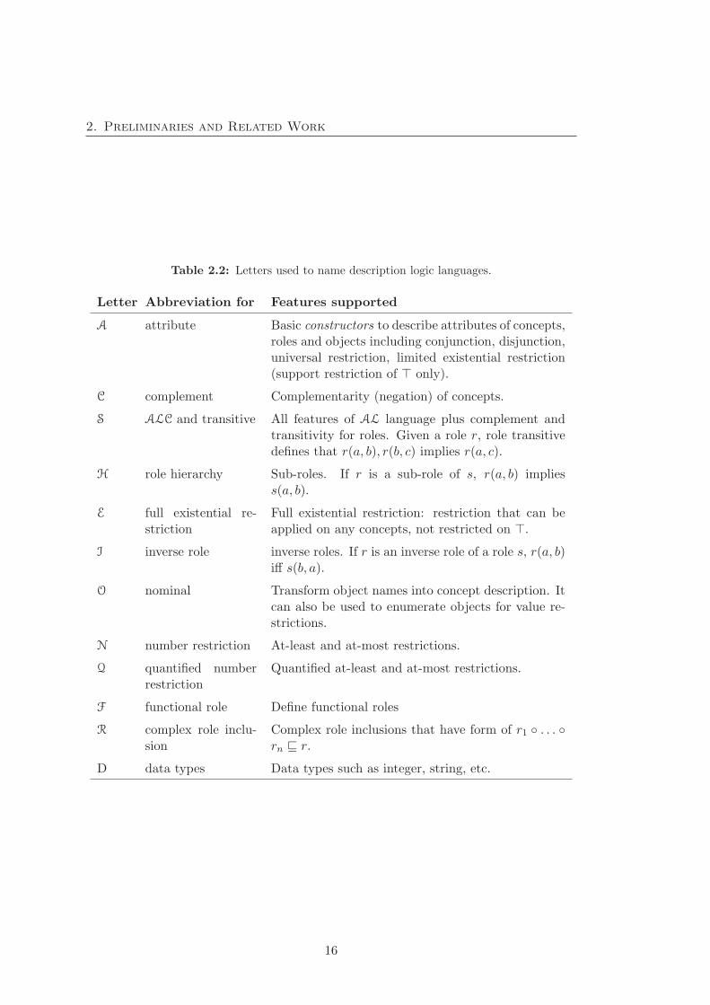
ported features. Table 2.2 provides a list of letters that are used to name the description
logic languages. For example, the description logic ALC is the attribute language with
complement. This is an extension of the AL language defined in Definition 2.1 that
adds support of negation, i.e. if C is a concept, ¬C is also a concept.
In this section, the syntax of two basic DL languages are provided: AL and SRIOQ.
AL is the most basic language in description logics, which is the extension of all other
languages. SRIOQ is an underlying logic for the most-up-to-date W3C recommendation
for semantic web language OWL-DL [64]. Their syntaxes are defined below.
Definition 2.1 (Syntax of AL language). Let NC be a set of atomic concepts
(concept names) and NR be a set of roles names (NC and NR are disjoint). Concepts
in the AL language are defined as follows:
1. Every atomic concept C ∈ NC is a concept.
2. (top) and ⊥ (bottom) are concepts.
3. If C and D are concepts, and r is a role, the followings are also concepts:
• C �D (disjunction), C �D (conjunction),
• ∀r.C (universal restriction), ∃r.C (existential restriction). �
14

2. Preliminaries and Related Work
Table 2.1: Basic concept constructors in description logics. A,C,D are atomic concepts,r is a role name and n denotes an integer number.
Constructor Syntax Example
atomic concept concept name C,D, Person
role role name r, s, hasChild
top (TOP) concept -
bottom (BOTTOM) concept ⊥ -
conjunction � C �D
disjunction � C �D
complement ¬ ¬Cexistential restriction ∃ ∃r.Cuniversal restriction ∀ ∀r.Cat-least restriction ≥ ≥ n r
at-most restriction ≤ ≤ n r
qualified at-least restriction ≥ ≥ n r.C
qualified at-most restriction ≤ ≤ n r.C
The SROIQ language is more expressive than AL, but is still decidable. This
language is an extension of AL with more supported constructors including concept
complement, role transitivity, role inversion, nominals, qualified number restrictions
and complex role inclusions. Its syntax is defined as follows:
Definition 2.2 (Syntax of SRIOQ language). Let NC be a set of atomic concepts
(concept names), NC be a set of roles names and NI be a set of individuals (NC , NR
and NI are disjoint). Concepts in SROIQ language are defined as follows:
1. Every atomic concept C ∈ NC is a concept.
2. (top) and ⊥ (bottom) are concepts.
3. If C and D are concepts, r is a role, the followings are also concepts:
• C �D (disjunction), C �D (conjunction), ¬C,
• ∀r.C (universal restriction), ∃r.C (existential restriction),
• {a1, . . . , an}, with ai ∈ NI (nominal),
• ≥ n r.C, ≤ n r.C (qualified number restrictions). �
15
2. Preliminaries and Related Work
Table 2.2: Letters used to name description logic languages.
Letter Abbreviation for Features supported
A attribute Basic constructors to describe attributes of concepts,roles and objects including conjunction, disjunction,universal restriction, limited existential restriction(support restriction of only).
C complement Complementarity (negation) of concepts.
S ALC and transitive All features of AL language plus complement andtransitivity for roles. Given a role r, role transitivedefines that r(a, b), r(b, c) implies r(a, c).
H role hierarchy Sub-roles. If r is a sub-role of s, r(a, b) impliess(a, b).
E full existential re-striction
Full existential restriction: restriction that can beapplied on any concepts, not restricted on .
I inverse role inverse roles. If r is an inverse role of a role s, r(a, b)iff s(b, a).
O nominal Transform object names into concept description. Itcan also be used to enumerate objects for value re-strictions.
N number restriction At-least and at-most restrictions.
Q quantified numberrestriction
Quantified at-least and at-most restrictions.
F functional role Define functional roles
R complex role inclu-sion
Complex role inclusions that have form of r1 ◦ . . . ◦rn r.
D data types Data types such as integer, string, etc.
16
2. Preliminaries and Related Work
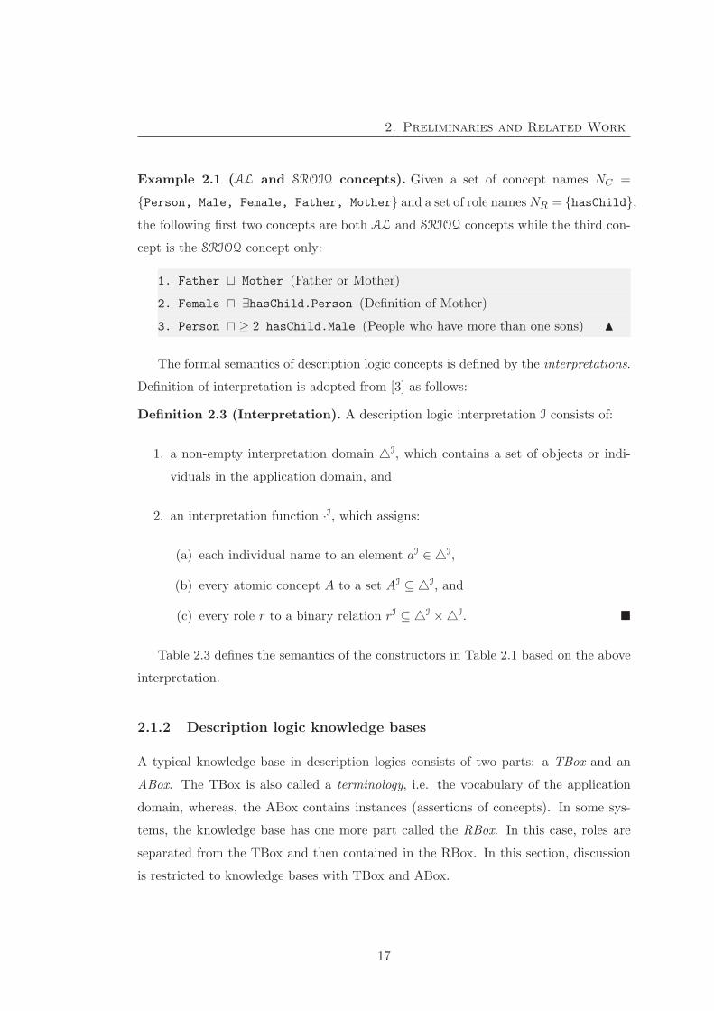
Example 2.1 (AL and SROIQ concepts). Given a set of concept names NC =
{Person, Male, Female, Father, Mother} and a set of role namesNR = {hasChild},the following first two concepts are both AL and SRIOQ concepts while the third con-
cept is the SRIOQ concept only:
1. Father � Mother (Father or Mother)
2. Female � ∃hasChild.Person (Definition of Mother)
3. Person � ≥ 2 hasChild.Male (People who have more than one sons) �
The formal semantics of description logic concepts is defined by the interpretations.
Definition of interpretation is adopted from [3] as follows:
Definition 2.3 (Interpretation). A description logic interpretation I consists of:
1. a non-empty interpretation domain �I, which contains a set of objects or indi-
viduals in the application domain, and
2. an interpretation function ·I, which assigns:
(a) each individual name to an element aI ∈ �I,
(b) every atomic concept A to a set AI ⊆ �I, and
(c) every role r to a binary relation rI ⊆ �I ×�I. �
Table 2.3 defines the semantics of the constructors in Table 2.1 based on the above
interpretation.
2.1.2 Description logic knowledge bases
A typical knowledge base in description logics consists of two parts: a TBox and an
ABox. The TBox is also called a terminology, i.e. the vocabulary of the application
domain, whereas, the ABox contains instances (assertions of concepts). In some sys-
tems, the knowledge base has one more part called the RBox. In this case, roles are
separated from the TBox and then contained in the RBox. In this section, discussion
is restricted to knowledge bases with TBox and ABox.
17

2. Preliminaries and Related Work
Table 2.3: The semantics of basic concept constructors in description logics.
Constructor Syntax Semantics
atomic concept A AI ⊆ �I
role r rI ⊆ �I ×�I
top (TOP) concept - �I
bottom (BOTTOM) concept - ∅conjunction C �D (C �D)I = CI ∩DI
disjunction C �D (C �D)I = CI ∪DI
complement ¬C (¬C)I = �I \ CI
existential restriction ∃r.C (∃r.C)I ={a | ∃b (a, b) ∈ rI ∧ b ∈ CI}
universal restriction ∀r.C (∀r.C)I ={a | ∀b (a, b) ∈ rI ⇒ b ∈ CI}
at-least restriction ≥ n r (≥ n r)I =
{a∣∣∣ ∣∣{b | (a, b) ∈ rI}∣∣ ≥ n}
at-most restriction ≤ n r (≤ n r)I =
{a∣∣∣ ∣∣{b | (a, b) ∈ rI}∣∣ ≤ n}
qualified at-least restriction ≥ n r.C (≥ n r.C)I =
{a∣∣∣ ∣∣{b | (a, b) ∈ rI}∣∣ ≥ n}
qualified at-most restriction ≤ n r.C (≤ n r.C)I =
{a∣∣∣ ∣∣{b | (a, b) ∈ rI}∣∣ ≤ n}
18
2. Preliminaries and Related Work
The TBox
The TBox of a knowledge base is usually stable. It contains a set of terminological
axioms that are defined as follows:
Definition 2.4 (Terminological axiom). Given two concepts C and D, a terminolog-
ical axiom has the form of an inclusion axiom C D or an equality axiom C ≡ D. �
An inclusion axiom is also called a subsumption axiom (C D is read “C is
subsumed by D”). Informally, this is an is-a relationship. An equality axiom is called
a definition if its left hand side is an atomic concept. An example of terminological
axioms is given below.
Example 2.2 (Axiom and definition). Given a set of concept names and role names
defined in Example 2.1, the following are some terminological axioms. The last axiom
is also a definition:
Woman Person
∃hasChild.Person ≡ Mother � Father
Father ≡ Male � ∃hasChild.Person �
The terminological axioms for roles are defined similarly, and can be found in [3].
The semantics (satisfaction) of inclusion and equality axioms are defined as follows:
Definition 2.5 (Satisfaction of axiom). Let I be an interpretation. Then:
• An inclusion axiom C D is satisfied by I if CI ⊆ DI.
• An equality axiom C ≡ D is satisfied by I if CI = DI. �
Informally, C D holds if all instances of C are instances of D, and C ≡ D if C
and D have the same set of instances, i.e. C D and D C. The above definition of
the axiom satisfaction can be extended to sets of axioms: An interpretation I satisfies
a set of axiom T if I satisfies all axioms in T. This leads to the definition of the concept
of a model.
Definition 2.6 (Model of a TBox). An interpretation I is called a model of an
axiom (respectively a set of axioms) A, denoted by I |= A, if I satisfies A (respectively
all axioms in A). I is called a model of a TBox if it satisfies all axioms in the TBox. �
19
2. Preliminaries and Related Work
Knowledge representation systems provide means not only for knowledge represen-
tation, but also for reasoning. The basic reasoning tasks on a TBox includes termi-
nology classification, logical implication and consistency checking. The first two tasks
are essentially based on the problem of checking subsumption and equivalence relations
between concepts. We introduce some basic concepts that support the above tasks as
follows (adopted from [3] and [82]):
Definition 2.7 (Consistency). A TBox is consistent if it has a model. �
Definition 2.8 (Satisfiability). A concept C is satisfiable with respect to a TBox
T if there is a model I of T such that CI is not empty. Otherwise, C is said to be
unsatisfiable. �
Definition 2.9 (Subsumption). A concept C is subsumed by a concept D with
respect to the TBox T, denoted by C D if for any model I of T we have CI ⊆ DI. �
Definition 2.10 (Equivalence). A concept C is equivalent to a concept D with re-
spect to a TBox T, denoted by C ≡ D, if for any model I of T we have CI = DI. �
Checking the satisfiability of a concept is the most is the most common task in
TBox reasoning. Some other reasoning tasks such as checking equivalence, disjointness,
or subsumption, can be reduced to the checking for satisfiability/unsatisfiability. For
instance, a concept C is subsumed by a concept D if and only if C�¬D is unsatisfiable,
or C and D are disjoint if and only if C �D is unsatisfiable.
The ABox
An ABox contains assertions including concept assertions and role assertions. Concept
assertions represent objects in the domain of discourse and role assertions represent re-
lationships between objects. A concept assertion has the form C(a) and a role assertion
has the form r(b, c), where a, b and c denote individual names, C is a concept and r
is a role. Knowledge in an ABox usually depends upon particular circumstances and
thus it is subject to change more often than the TBox.
Example 2.3 (Assertion in the ABox). Given a set of concept names NC and role
names NR described in Example 2.1 and a set of individuals NI = {john,mary, tom},the following is an example of an ABox that contains concept and role assertions:
20
2. Preliminaries and Related Work
ABox A = {Male(john)
Male(tom)
Female(mary)
hasChild(john, tom)
hasChild(mary, tom)
} �
Similar to the TBox, there are also some reasoning tasks on ABoxes. The most basic
reasoning tasks on an ABox are consistency checking, instance checking and instance
retrieval. Before describing these task, we introduce some related concepts:
Definition 2.11 (Assertions satisfaction). An interpretation I is said to satisfy :
• a concept assertion C(a) if aI ∈ CI,
• a role assertion r(a, b) if (aI, bI) ∈ rI, and
• an ABox A if it satisfies all assertions in A. �
Similarly, an interpretation I is said to satisfy an assertion A (concept or role) with
respect to a TBox T if it is satisfies both A and T. Then, the concept model of an ABox
is defined as follows:
Definition 2.12 (Model of an ABox). An interpretation is called a model of:
• an ABox A if it satisfies all assertions in A, and
• an ABox A with respect to a TBox T if it is a model of both A and T. �
The consistency of an ABox and basic tasks in the ABox can now be defined as
follows:
Definition 2.13 (Consistency). An ABox A is consistent if it has a model and
consistent with respect to a TBox T if there exists an interpretation that is a model of
both A and T. �
Definition 2.14 (Instance check). Given a knowledge base K = (T,A), a concept C
and an individual name a ∈ NI , a is an instance of C with respect to K, denoted by
K |= C(a), iff for any models I of K (i.e. model of both A and T), we have aI ∈ CI. �
21

2. Preliminaries and Related Work
An instance check problem can be defined based on the definition of consistency:
K |= C(a) if K ∪ {¬C(a)} is inconsistent. If a is not an instance of a concept C with
respect to a knowledge base K, it is denoted by K � C(a).
Definition 2.15 (Instance retrieval). Given a concept C, an instance retrieval prob-
lem for C with respect to a knowledge base K is to find all individuals a such that
K |= C(a). �
Example 2.4 (DL knowledge base and reasoning tasks). Given a set of concept
names NC and a set of role names NR in Example 2.1; a set of individuals NI in
Example 2.3; and the knowledge base K = (T,A) and an interpretation I as follows:
TBox T = {Woman Person
∃hasChild.Person ≡ Mother � Father
Father ≡ Male � ∃hasChild.Person}ABox A = {
Male(john)
Male(tom)
Female(mary)
hasChild(john, tom)
hasChild(mary, tom)
}Interpretation I = {
�I = {JOHN, MARY, TOM} (objects in the application domain)
johnI = JOHN, (tom)I = TOM, maryI = MARY
PersonI = { JOHN, MARY, TOM }FemaleI = { MARY }MaleI = { JOHN }FatherI = { JOHN }MotherI = ∅hasChildI = { (JOHN, TOM), (MARY, TOM) }
}
22
2. Preliminaries and Related Work
Then, I does not satisfy the ABox A as it does not satisfy the assertion Male(tom)
as tomI /∈ MaleI (TOM /∈ {JOHN}). I also does not satisfy the TBox T as it does not
satisfy the following axiom:
∃hasChild.Person ≡ Mother � Father
because:
∃hasChild.PersonI = {JOHN, MARY} �= (Mother � Father)I = {JOHN}.Consider an interpretation I1 is the same I with one modification MaleI = { JOHN,
TOM }. I1 is now satisfy A as it satisfies all assertions in A (I is now satisfies Male(john)
as johnI ∈ MaleI). However, it still does not satisfy T.
Given another interpretation I2 is the same I1 with one modification that the map-
ping Mother is modified to MotherI = {MARY}, I2 satisfies both A and T as it now
satisfies the equality axiom ∃hasChild.Person ≡ Mother � Father:
∃hasChild.PersonI = {JOHN, MARY}= (Mother � Father)I = {JOHN, MARY}.In this case, I2 is also a model of K. �
2.1.3 The Web Ontology Language (OWL)
The Web Ontology Language (OWL) is a W3C recommendation for the Semantic Web
[14, 96]. This is a family of languages that are based on description logics. OWL
has some additional features to integrate it with other web standards such as Uniform
Resource Identifier (URI) [97] and to address specific use cases, such as imports of
external knowledge bases, and support for Resource Description Framework (RDF)
and Resource Description Framework Schema (RDFS) [91, 95]. In addition, OWL also
uses a different terminology (closer to the object-oriented terms) for the basic concepts
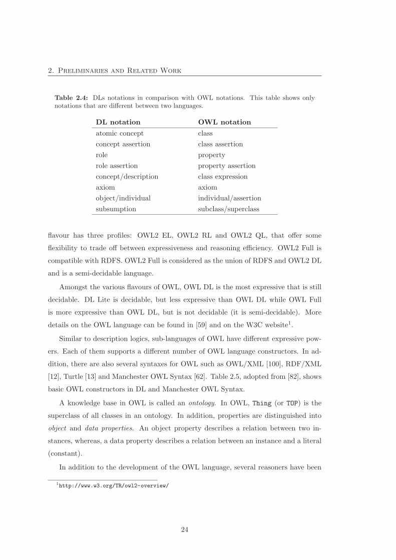
defined in description logics. Table 2.4 summarises this correspondence.
The first version of OWL included three flavours: OWL Lite, OWL DL and OWL
Full [96]. The first two languages are based on the SHIF(D) and SHOIN(D) description
logic respectively. OWL Full supports some features of RDFS that are beyond the
expressive power of description logics. It is considered as the union of OWL DL and
RDFS, a schema language of the Semantic Web.
The most up-to-date version of OWL is OWL2, which comes in two flavours: OWL2
DL and OWL2 Full [59, 100]. OWL2 DL is based on the SROIQ(D) language. This
23
2. Preliminaries and Related Work
Table 2.4: DLs notations in comparison with OWL notations. This table shows onlynotations that are different between two languages.
DL notation OWL notation
atomic concept class
concept assertion class assertion
role property
role assertion property assertion
concept/description class expression
axiom axiom
object/individual individual/assertion
subsumption subclass/superclass
flavour has three profiles: OWL2 EL, OWL2 RL and OWL2 QL, that offer some
flexibility to trade off between expressiveness and reasoning efficiency. OWL2 Full is
compatible with RDFS. OWL2 Full is considered as the union of RDFS and OWL2 DL
and is a semi-decidable language.
Amongst the various flavours of OWL, OWL DL is the most expressive that is still
decidable. DL Lite is decidable, but less expressive than OWL DL while OWL Full
is more expressive than OWL DL, but is not decidable (it is semi-decidable). More
details on the OWL language can be found in [59] and on the W3C website1.
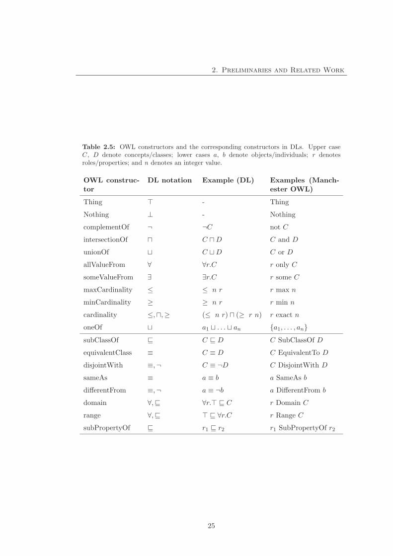
Similar to description logics, sub-languages of OWL have different expressive pow-
ers. Each of them supports a different number of OWL language constructors. In ad-
dition, there are also several syntaxes for OWL such as OWL/XML [100], RDF/XML
[12], Turtle [13] and Manchester OWL Syntax [62]. Table 2.5, adopted from [82], shows
basic OWL constructors in DL and Manchester OWL Syntax.
A knowledge base in OWL is called an ontology. In OWL, Thing (or TOP) is the
superclass of all classes in an ontology. In addition, properties are distinguished into
object and data properties. An object property describes a relation between two in-
stances, whereas, a data property describes a relation between an instance and a literal
(constant).
In addition to the development of the OWL language, several reasoners have been
1http://www.w3.org/TR/owl2-overview/
24
2. Preliminaries and Related Work
Table 2.5: OWL constructors and the corresponding constructors in DLs. Upper caseC, D denote concepts/classes; lower cases a, b denote objects/individuals; r denotesroles/properties; and n denotes an integer value.
OWL construc-tor
DL notation Example (DL) Examples (Manch-ester OWL)
Thing - Thing
Nothing ⊥ - Nothing
complementOf ¬ ¬C not C
intersectionOf � C �D C and D
unionOf � C �D C or D
allValueFrom ∀ ∀r.C r only C
someValueFrom ∃ ∃r.C r some C
maxCardinality ≤ ≤ n r r max n
minCardinality ≥ ≥ n r r min n
cardinality ≤,�,≥ (≤ n r) � (≥ r n) r exact n
oneOf � a1 � . . . � an {a1, . . . , an}subClassOf C D C SubClassOf D
equivalentClass ≡ C ≡ D C EquivalentTo D
disjointWith ≡,¬ C ≡ ¬D C DisjointWith D
sameAs ≡ a ≡ b a SameAs b
differentFrom ≡,¬ a ≡ ¬b a DifferentFrom b
domain ∀, ∀r. C r Domain C
range ∀, ∀r.C r Range C
subPropertyOf r1 r2 r1 SubPropertyOf r2
25
2. Preliminaries and Related Work
developed to provide reasoning service for OWL knowledge bases. Similar to description
logics, reasoning in OWL includes classification, checking for the consistency of knowl-
edge bases, checking for the satisfiability of axioms (descriptions/concepts), checking
for subsumption relationships and instance checking. Some popular OWL reasoners
are RacerPro [56], Pellet [107], FaCT [63], and HerMiT [117]. Some of them, such as
RacerPro and Pellet, also provide justification (or explanation/trace) for inferences or
inconsistency checks [38, 71]. This feature is useful for debugging ontologies and to
increase the trust in inferred knowledge.
2.2 Description Logic and OWL Learning
Description logic learning has its roots in inductive logic programming [101, 104]. In
description logic learning, description logics are used as the knowledge representation
language. The essential idea of induction is to obtain principles from experiences [8,
9]. The idea was employed in machine learning with different names before it was
first named Inductive Logic Programming by Stephen Muggleton in 1990 [101]. Then,
induction was employed in description logics [6, 31, 85] and it obtained more attention
when the semantic web became widely used [79, 83, 143].
2.2.1 Description logic learning problem
Since OWL has its root in description logics, learning problem in OWL and DLs shares
similar concepts and notations. Therefore, DL and OWL learning are used interchange-
ably. A description logic learning problem can be described as follows:
Definition 2.16 (Description logic learning). Given a knowledge base K and a
set of positive E+ and negative E− examples such that E+ ∩ E− = ∅, description logic
learning aims to find a concept C such that K |= C(e) for all e ∈ E+ (complete) and
K � C(e) for all e ∈ E− (consistent/correct). �
A description logic learning problem can be described as a structure 〈K, (E+,E−)〉where K is a knowledge base (ontology), E+ is a set of positive examples and E− is a
set of negative examples. A learnt concept is also called a hypothesis or definition.
Notation |= is defined in Definition 2.14 to denote an instance checking problem.
26

2. Preliminaries and Related Work
K |= C(a) denotes a is an instance of class C with respect to the knowledge base K.
If K |= C(a) is satisfied, C is also said to cover a with respect to K.
The learning problem described in Definition 2.16 is called learning from positive
and negative examples. It is distinguished from two other learning problems: learning
from positive examples only, and concept learning. One of the approaches to learn
from positive examples only is to transform it into learning from positive and negative
examples problem by considering negative examples as the set of {e ∈ K | e /∈ E+}where E+ is a set of positive examples. In concept learning, a concept name is provided.
All instances of the given concept are used as positive examples and instances of other
classes in the knowledge base are used as negative examples.
In this thesis, the discussion is restricted to the positive and negative examples
learning problem. An example of a description logic learning problem is given below.
Example 2.5 (Description logic learning problem). Given an ontology (in Manch-
ester OWL syntax):
• TBox:
Class: Person SubClassOf: Thing
Class: Male SubClassOf: Person
Class: Female SubClassOf: Person
ObjectProperty: hasChild
Domain: Person, Range: Person
• ABox (assertions):
Individual: john Types: Male
Facts: hasChild tom
Individual: mary Types: Female
Facts: hasChild tom
Individual: tom Types: Male
Individual: eve Types: Female
Individual: peter Types: Male
Facts: hasChild mary
27
2. Preliminaries and Related Work
and a set of positive examples E+ = {john, peter} (who are fathers) and negative
examples E− = {mary, tom, eve} (who are not fathers). The following concept can be
produced by a typical inductive description logic learning algorithm that describes the
family relationship Father :
Male and hasChild some Person
Similarly, if E+ = {john, peter,mary} (parents) and E− = {tom, eve} (who are not
parents), the following concept can be produced that describes the family relationship
Parent :
hasChild some Person
�
Some properties of a learnt concept are defined below:
Definition 2.17 (Complete, correct and accurate concepts). Given a description
logics learning problem P = 〈K, (E+,E−)〉 and a concept C learnt from P, C is:
• complete with respect to P if K |= C(e) for all e ∈ E+,
• correct with respect to P if K � C(e) for all e ∈ E−, and
• accurate if C is both complete and correct. �
Definition 2.18 (Incomplete and incorrect concepts). Given a description logic
learning problem P = 〈K, (E+,E−)〉 and a concept C learnt from P, C is:
• incomplete with respect to P if ∃e ∈ E+ such that K � C(e), and
• incorrect with respect to P if ∃e ∈ E− such that K |= C(e) �
Definition 2.19 (Overly general and overly specific concepts). Given a descrip-
tion logic learning problem P = 〈K, (E+,E−)〉 and a concept C learnt from P :
• C is overly general if it is complete but incorrect.
• C is overly specific if it is correct but incomplete. �
28
2. Preliminaries and Related Work
Example 2.6 (Overly general and overly specific concept). Given a background
as in Example 2.5, a set of positive examples E+ = {john, peter,mary} (parents) and
E− = {tom, eve} (who are not parents). Then, the concept:
• Person is overly general as it is complete (covers all positive examples) and in-
correct (covers some negative examples).
• Male AND hasChild SOME Person is overly specific as it correct (covers no neg-
ative examples) and incomplete (does not cover all positive examples). �
2.2.2 Basic approaches in DL learning
Learning in description logics is essentially a search problem: it searches for an accurate2
concept in a search space that consists of a potential infinite set of concepts constructed
from the vocabulary of language of a given knowledge base. Concepts in the search
space are generated by refinement operators and they are organised in an ordering
structure.
There are two types of refinement operator: downward and upward refinement
operators. Given a concept, a downward refinement operator computes a set of concepts
that aremore specific than the given concept. An upward refinement operator computes
a set of concepts that are more general than the given concept. In description logics
and OWL, the generality and specificity relations between concepts are based on the
inclusion (subclass/superclass) relationship. A description C subsumes a description
D (or C is a superclass of D) if all instances of D are also instances of C. Therefore,
C is said to be more general than D, or D is more specific than C. C is called a
generalisation of D and D is a specialisation of C. A refinement operator based on
these relations can be defined as follows:
Definition 2.20 (Refinement operator in description logics). Given a descrip-
tion logic language L and a concept C in L. A downward (respectively upward)
refinement operator ρ is a mapping from C to a set of concepts D in L such that
∀D ∈ D : D C (respectively C D). D is called refinement of C. �
2Complete and correct
29

2. Preliminaries and Related Work
Definition 2.20 implies that the refinement process can be applied recursively and
it may be infinite. Therefore, practically, a refinement task is often provided with a
maximal length of the concepts in the refinement result to help the refinement become
finite. There are several methods to define concept length. In this thesis, the concept
length computation is adopted from [82] as follows:
Definition 2.21 (Length of a concept in description logics). The length of a
concept in description logics is the total number of symbols in the concept including
class names, role names, individual, and constructors. �
In particular, the length of an ALC concept is defined as follows:
Definition 2.22 (Length of an ALC concept). The length of a concept C, denoted
by |C|, is inductively defined as follows:
|A| = || = |⊥| = 1 (A is an atomic concept)
|¬D| = 1 + |D|D � E = |D � E| = 1 + |D|+ |E||∀r.D| = |∃r.D| = 2 + |D| �
Corresponding to two types of refinement operator, there are two basic search di-
rections: top-down and bottom-up. It results in the two basic inductive learning ap-
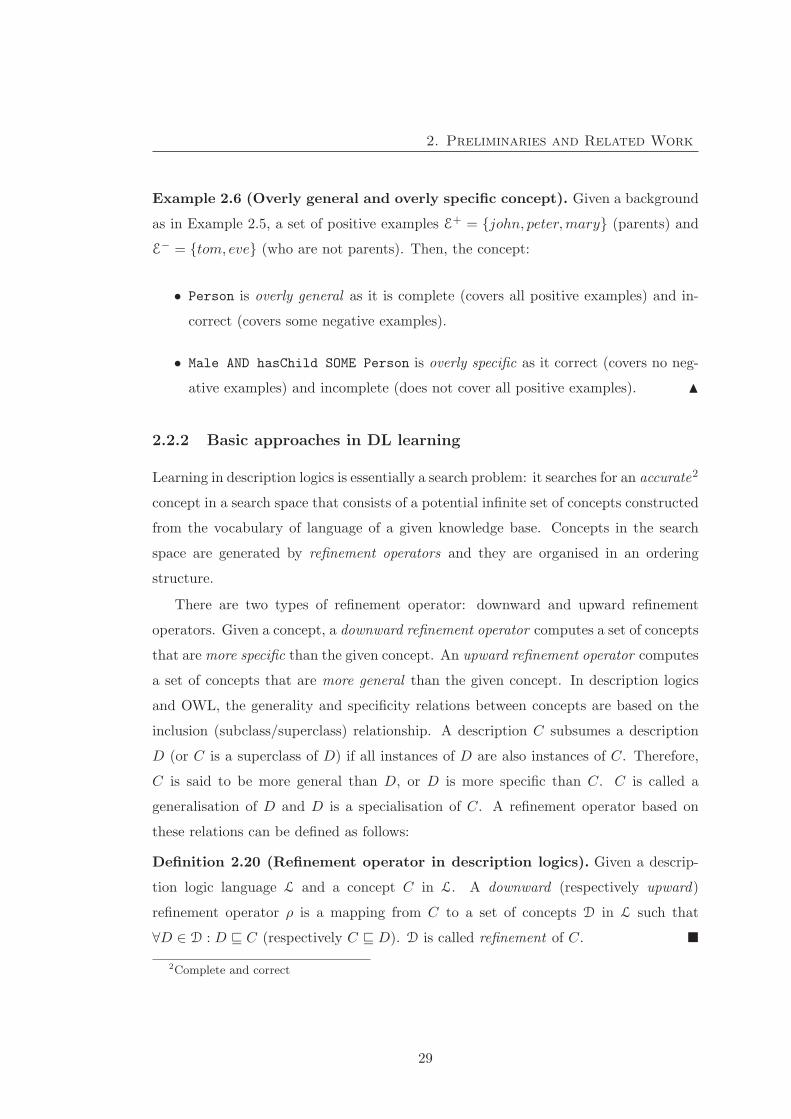
proaches: top-down and bottom-up approach respectively.
Top-down (specialisation) approach
In the top-down learning approach, the search starts from a general concept, usually
the Thing (TOP), and uses a downward refinement operator to specialise concepts in
the search space until a concept or set of concepts that cover all positive examples and
no negative ones is found. The basic tasks of a downward refinement are:
• replacing primitive concepts and properties in the description by their sub-concepts
or sub-properties, and
• specialising the range of properties, and
• adding more primitive concepts and properties into the description.
30
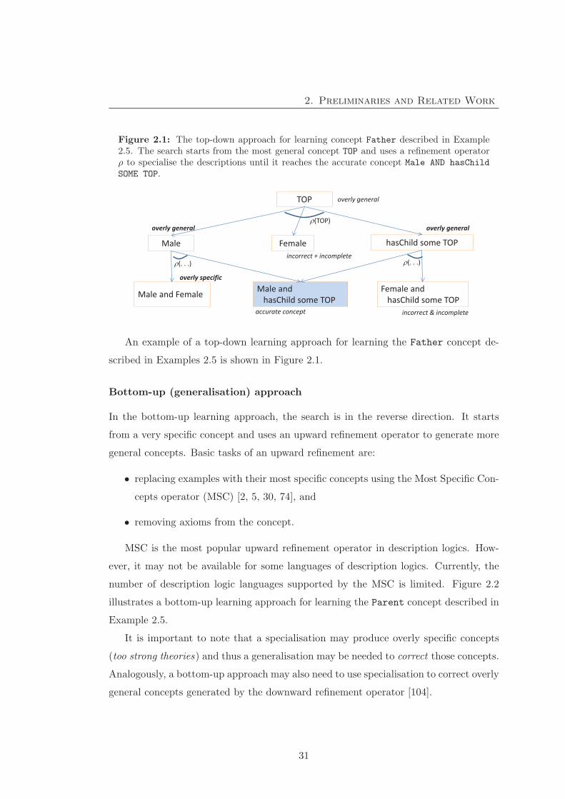
2. Preliminaries and Related Work
Figure 2.1: The top-down approach for learning concept Father described in Example2.5. The search starts from the most general concept TOP and uses a refinement operatorρ to specialise the descriptions until it reaches the accurate concept Male AND hasChild
SOME TOP.
(. . .)
TOP
Male Female hasChild some TOP
Male and Female Male and hasChild some TOP
Female and hasChild some TOP
overly general
overly general overly general
accurate concept incorrect & incomplete
overly specific
incorrect + incomplete
(TOP)
(. . .)
An example of a top-down learning approach for learning the Father concept de-
scribed in Examples 2.5 is shown in Figure 2.1.
Bottom-up (generalisation) approach
In the bottom-up learning approach, the search is in the reverse direction. It starts
from a very specific concept and uses an upward refinement operator to generate more
general concepts. Basic tasks of an upward refinement are:
• replacing examples with their most specific concepts using the Most Specific Con-
cepts operator (MSC) [2, 5, 30, 74], and
• removing axioms from the concept.
MSC is the most popular upward refinement operator in description logics. How-
ever, it may not be available for some languages of description logics. Currently, the
number of description logic languages supported by the MSC is limited. Figure 2.2
illustrates a bottom-up learning approach for learning the Parent concept described in
Example 2.5.
It is important to note that a specialisation may produce overly specific concepts
(too strong theories) and thus a generalisation may be needed to correct those concepts.
Analogously, a bottom-up approach may also need to use specialisation to correct overly
general concepts generated by the downward refinement operator [104].
31
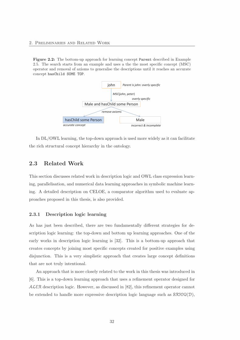
2. Preliminaries and Related Work
Figure 2.2: The bottom-up approach for learning concept Parent described in Example2.5. The search starts from an example and uses a the the most specific concept (MSC)operator and removal of axioms to generalise the descriptions until it reaches an accurateconcept hasChild SOME TOP.
john
Male and hasChild some Person
hasChild some Person Male
MSC(john, peter)
Parent is john: overly specific
remove axioms
overly specific
accurate concept incorrect & incomplete
In DL/OWL learning, the top-down approach is used more widely as it can facilitate
the rich structural concept hierarchy in the ontology.
2.3 Related Work
This section discusses related work in description logic and OWL class expression learn-
ing, parallelisation, and numerical data learning approaches in symbolic machine learn-
ing. A detailed description on CELOE, a comparator algorithm used to evaluate ap-
proaches proposed in this thesis, is also provided.
2.3.1 Description logic learning
As has just been described, there are two fundamentally different strategies for de-
scription logic learning: the top-down and bottom up learning approaches. One of the
early works in description logic learning is [32]. This is a bottom-up approach that
creates concepts by joining most specific concepts created for positive examples using
disjunction. This is a very simplistic approach that creates large concept definitions
that are not truly intentional.
An approach that is more closely related to the work in this thesis was introduced in
[6]. This is a top-down learning approach that uses a refinement operator designed for
ALER description logic. However, as discussed in [82], this refinement operator cannot
be extended to handle more expressive description logic language such as SRIOQ(D),
32
2. Preliminaries and Related Work
which is the language on which OWL2 is based.
Lisi [85] has proposed an alternative top-down approach based on the hybrid AL-log
language, which combines the ALC description logic language and Datalog. An ideal
downward refinement operator [104] for AL-log language was proposed that is based on
the notation of B-subsumption. This is a generalisation of the generalised subsumption
to the AL-log language. This approach is suitable for the hybrid knowledge represen-
tation systems that are constituted by the relational and structural subsystems. This
approach was implemented in the A-QuIn (AL-log Query Induction) system.
In [43, 66], a top-down refinement operator for the ALC language is used in com-
bination with a bottom-up MSC operator. The essential idea of these studies lies in
the concept of counterfactual. This can be considered as the errors within candidate
hypotheses. Therefore, for each candidate hypothesis, the learning algorithm uses a
MSC operator to find the concept(s) representing errors and remove them from the
candidate hypothesis. However, this approach has two disadvantages: i) the finding of
concept(s) for counterfactuals may be repeated for a same set of errors, and ii) as a
result, it tends to generate unnecessarily long concepts.
The most recent description logic learning algorithms have been proposed in [80].
Two top-down refinement operators have been proposed. One is for the EL language
and the other is for ALC (although it can be extended to more expressive languages).
The latter is the most expressive refinement operator proposed so far. In addition,
several learning approaches based on the proposed refinement operators were also de-
veloped. Two interesting algorithms in this framework are Class Expression Learner for
Ontology Engineering (CELOE) and OWL Class Expression Learner (OCEL). These
algorithms are evaluated and compared very well with other learning approaches [57].
However, they are sequential algorithms and thus they cannot take advantages of par-
allel systems such as multi-core processors, or cloud computing platforms. In addition,
these algorithms focus on generating short descriptions and thus they have another dis-
advantage: they cannot handle complex learning problems (see [57] and the evaluation
in Chapter 5).
DL-FOIL [45] combines both top-down and bottom-up learning. The top-down
step finds a set of correct concepts such that each of them correctly defines a subset of
33
2. Preliminaries and Related Work
the positive examples. Then, the bottom-up step computes a complete concept that
defines all positive examples. This approach handles complex concepts better than
the top-down or bottom-up approach alone. However, it produces longer concepts
in comparison with the approaches proposed in [80]. The unnecessarily long learnt
concepts are caused by the lack of optimisation in the aggregation step. In addition,
like other existing description logic learning algorithms, this approach is serial by nature
and thus it cannot take advantage of concurrency.
2.3.2 Parallel description logic learning
Parallel computing has a long history of development from the late 1950s, from multi-
processor computer systems, to multi-core processors. Parallelisation helps to use the
computer resources more effectively in order to: i) create fast and efficient algorithms, ii)
create highly scalable algorithms. Currently, parallelisation can be found in every area
of computing with many parallel frameworks developed such as Parallel Virtual Machine
(PVM) [126], Apache Hadoop [15] and applications/systems that use parallelisation.
In logics, parallelisation has been used to develop parallel logic programming lan-
guages such as PARLOG [53] and PEPSys [111]. These research relate to the paralleli-
sation for logic deduction.
In inductive logic programming, a parallel inductive logic programming approach
was proposed in [37]. The basic idea of this approach is to partition positive examples
into several sets depending on the parallel level of the system. Concepts for the par-
titioned sets are combined at the end. In [93], several parallelisation strategies were
implemented in FOIL, an inductive logic learning algorithm [108]. These strategies
mainly differ in the dividing strategies. The first strategy divides search space among
processors, i.e. the multiple refinements work in parallel. The second strategy is similar
to [37], i.e. examples are partitioned into several sets and they are learnt independently.
In the last strategy, examples are divided based on the background knowledge. Inde-
pendent examples are divided into different sets. Our parallel learning approach is
similar to the first strategy. We explore the search space in parallel. However, our
approach is different from this approach with respect to the learning strategy used:
we employ concepts for a subset of positive examples and use a reduction strategy to
34
2. Preliminaries and Related Work
construct the final concept. In addition, our learning approach uses description logic
instead.
In description logics, parallelisation is also used. However, the use of parallelisation
is limited in parallel description logic reasoning with some parallel description reasoners
developed such as Deslog reasoner [141], or parallel inferencing algorithms for OWL
[84, 122]. There is no parallel description logic learning algorithm proposed so far.
2.3.3 Numerical data learning in description logics
Amongst the existing description and class expression learning algorithms such as AL-
QuIn [85], DL-FOIL [45], YinYang [66] and a set of learning algorithms in the DL-
Learner framework such as CELOE, OCEL, ELTL [80], numeric data property learning
strategy was only explicitly described and supported by the algorithms in DL-Learner
framework. In these algorithms, a fixed-size segmentation strategy is used to compute a
set of values used for refinement of numerical data. In this method, a maximal number
of values for refining numerical data is assigned. Then, the numerical values are split
into equal parts according to the maximal number of values allowed and the middle
values of split parts are used for the refinement. This strategy can reduce the number
of values used for refinement and therefore it can reduce the search space. However,
this strategy may remove some meaningful values from the refinement.
In inductive logic programming, the root of description logic learning, many other
strategies were proposed. For example, in Aleph, several strategies were supported such
as guessing the values used for refinement or using lazy evaluation (this strategy has not
been described in detail), etc. [123]. However, it was reported that these approaches
do not always work. Fixed increment and decrement are also used in Aleph. This is
used more commonly for integer datatypes. For example, the value of an attribute is
increased or decreased by a fixed value, e.g. 1, 2, etc. in each refinement step. Closer to
our approach, a modification of discretisation method proposed in [46] was used in the
Inductive Constraint Logic (ILC) system [133]. The essential idea of discretisation of
continuous data proposed in [46] is based on information entropy. Potential cut points
(segmentations) are estimated using a class entropy function. However, when this
approach was used in ILC, it was reported that very few subintervals were generated
35
2. Preliminaries and Related Work
and therefore they combined discretisation approach with a fixed numbers of values
desired to be generated, e.g. 10 values or 20 values, etc.
2.3.4 Class Expression Learner for Ontology Engineering (CELOE)
CELOE is a top-down OWL class expression learning algorithm in the DL-Learner
framework, which is the most recently developed OWL class expression learning al-
gorithm [82]. This algorithm uses a downward refinement operator that supports the
ALC description logic language to specialise the descriptions in the search space. The
implementation of this refinement operator was extended to support more expressive
power such as datatype (D) and number restrictions (N).
As a typical top-down description logic learning approach, this algorithm starts
from a general concept, the TOP concept by default, and uses the refinement operator
to generate descriptions in the search space until an accurate description found. The
selection of descriptions in the search space for refinement (expansion) is based on the
score of a description, which is mainly based on the descriptions’ accuracy. The score
of a description C is defined as follows:
score(C) = accuracy(C) + 0.2× accuracy gain(C)− 0.05× n
where accuracy(C ) is the accuracy of description C (see Definition 3.2); accuracy gain(C )
is the difference between accuracy of C and its parent; and n is the horizontal expansion
of C.
The horizontal expansion of a description is the sum of its length and the number of
times it was refined. A description in the search space may be refined many times. The
refinement operator is only allowed to produce descriptions with a length that is shorter
or equal the horizontal expansion of the refined description. This is a mechanism used
to deal with the infinite property of the refinement operator. As this algorithm finds
single descriptions that describes all positive examples, overly specific descriptions are
ignored, i.e. they are not added into the search space for further refinement (expansion).
This algorithm was implemented and distributed with DL-Learner, an open source
machine learning framework. It was well evaluated and compared with popular de-
36

2. Preliminaries and Related Work
scription learning algorithms. The evaluation shows that this is a promising OWL class
expression learning algorithm that produce very concise (short and readable) concepts
[57]. However, as this algorithm only uses the top-down learning approach, it cannot
deal well with complex learning problems that require long descriptions to describe the
positive examples.
37

2. Preliminaries and Related Work
38
Chapter 3
Evaluation Methodology
This chapter describes the evaluation methodology of the proposed algorithms
in this study. We first provide a description of evaluation metrics. Next,
there is a detailed account of our experimental framework including a cross-
validation procedure, a statistical significance test method. The control of the
algorithm terminations is also discussed. The chapter ends with the introduc-
tion of comparison algorithms and evaluation datasets.
3.1 Introduction
As was described in the introductory chapter, this thesis proposes four new approaches
to description logic learning. The aim of the approaches is to improve the learning
speed, the capability to deal with complex learning problems, and the flexibility to
trade off the predictive correctness and completeness.
In this chapter, we describe the evaluation methodology for our proposed algo-
rithms. A thorough evaluation includes running the algorithms on selected datasets
and gathering interested metrics that help to reflect achievements of the proposed algo-
rithms. Then, the experimental results are compared with existing algorithms to assess
the achievements of our algorithms. Therefore, the evaluation methodology includes
the selections of: i) evaluation metrics (described in Section 3.2), ii) a method for mea-
suring the evaluation metrics and comparison with existing algorithms (described in
39
3. Evaluation Methodology
Section 3.3.1), iii) some existing algorithms for comparison with our algorithms (de-
scribed in Section 3.3.2), and iv) a set of evaluation datasets (described in Section
3.3.3).
3.2 Evaluation Metrics
Selected evaluation metrics must reflect the essential features of the evaluation algo-
rithms. In machine learning, predictive accuracy is the most important metric. It
represents the predictive power of the learnt concepts. However, it is useful to have a
more thorough assessment of a learning algorithm. Based on the aims of this thesis we
are also interested in learning time, search space size and definition length. The learning
time represents the speed of an algorithm, whereas the search space size indicates the
effectiveness of the memory usage. The last metric, definition length, provides a mea-
sure of the readability of the definition (in general, short definitions are more readable
than long definitions). Computation of these metrics is defined below.
3.2.1 Accuracy
Accuracy is a combination of completeness and correctness. In Definition 2.17, com-
plete, correct and accurate concepts were defined. However, that definition is used to
assess these metrics qualitatively, i.e. whether a concept is complete or incomplete,
correct or incorrect and accurate or inaccurate. We are defining these metrics in a
different context: for measuring the amount of completeness, correctness and accuracy.
Before introducing the calculation of these metrics, we restate the definition of instance
retrieval (see Definition 2.15) in form of a formula to simplify the use of this task.
Definition 3.1 (Cover). Let P = 〈K, (E+,E−)〉 be a learning problem defined in
Definition 2.16, E = (E+,E−) and C be a concept. Then, cover(K, C,E) is a function
that computes a set of examples covered by C with respect to K and is defined as:
cover(K, C,E) = {e ∈ E | e is covered by C with respect to K} �
The calculation of the completeness, correctness and accuracy can now be defined.
40
3. Evaluation Methodology
Definition 3.2 (Completeness, correctness and accuracy). Let P = 〈K, (E+,E−)〉be a learning problem. Then,
• completeness is the ratio of positive examples covered by C to the total number
of positive examples:
completeness(C,P ) =|cover(K, C,E+)|
|E+|
• correctness is the ratio of negative examples uncovered by C to the total numbers
of negative examples:
correctness(C,P ) = 1− |cover(K, C,E−)||E−|
=|E− \ cover(K, C,E−)|
|E−|
• accuracy is the ratio of number of positive examples covered by C and the number
of negative examples uncovered by C to the total number of all examples:
accuracy(C,P ) =|cover(K, C,E+)|+ |E− \ cover(K, C,E−)|
|E+ ∪ E−| �
Accuracy with respect to training data is called training accuracy and accuracy
with respect to test data is called predictive accuracy.
3.2.2 Learning time
The learning time of a learning algorithm is counted from when it starts to search for a
definition until the definition is found or the timeout is reached. The time for loading
the knowledge base into the reasoner is not counted. There are two basic methods to
measure learning time: using wall-clock time, the actual time that elapses from start to
end of a learning task; and using CPU time, which measures only the actual time that
the CPU works on the learning task. Technically, computation of CPU time is more
complicated than wall-clock time. However, if the evaluation system has constant loads,
wall-clock time is approximately equal to CPU time. Therefore, in our experiments,
41
3. Evaluation Methodology
we compute learning time using wall-clock time. To ensure the system has constant
loads, we can manually observe then system loads while the learners is running.
3.2.3 Definition length
The calculation of this metric was defined in Definitions 2.21 and 2.22. It is the total
number of symbols that appear within the definition excluding punctuations such as
“(”, “)”, “.” and “,”. For example, the length of the following definition is 5:
Male � ∃hasChild.Person
(or in Manchester OWL syntax: Male AND hasChild SOME Person).
In our implementation, the nomalisation procedure in the DL-Learner framework
is used to normalise the learnt definition.
3.2.4 Search space size
Search space size is the total number of descriptions generated by the refinement opera-
tor(s). This metric is used to assess the memory consumption of the learning algorithms,
also relates to learning time. Given the same learning problem, a learning algorithm
that can find a solution with a smaller search space than others is considered to have a
better search strategy. It also influences the scalability of a learning algorithm as using
the memory more effectively allows the algorithm to deal better with bigger (knowledge
base size, search tree size, etc.) learning problems.
3.3 Experimental Design
Our experimental design aims to produce reliable experimental results, fair comparisons
and accurate assessments of the achievement of our algorithms. The following sections
will describe methods to achieve these expectations.
3.3.1 Experimental framework
Evaluation of selected algorithms on a set of datasets includes running the experiment
for each algorithm on each dataset and measuring the relevant evaluation metrics. The
42
3. Evaluation Methodology
experimental results of the selected algorithms will be compared with each other and
the statistically significant differences will be computed. Therefore, four questions need
to be addressed in designing the experimental framework:
Q1. How many runs are sufficient to help the measurement of the evaluation metrics
to be reliable?
Q2. How to deal with small datasets (i.e. that have small number of examples)?
Q3. How to compare the experimental results and test for statistical significance?
Q4. How to control the termination of the learning algorithms in the case that there
is no accurate solution for the learning algorithm with respect to the dataset?
In the following sections, we will describe appropriate methods that answer the
above questions.
K-fold cross-validation (Q1 + Q2)
K-fold cross-validation is a popular evaluation method in machine learning. The basic
idea of this method is to partition the evaluation dataset into k sub-datasets and
repeat the experiment for each sub-dataset and measure the evaluation metrics of the
algorithm. Performing a k-fold cross-validation for a learning algorithm on a dataset
includes the following steps:
1. Randomly shuffle positive and negative examples in the dataset.
2. Divide examples into k equal-size parts, called sub-samples. If the number of
example in each example set is not divisible by k, size of the sub-samples may be
slightly different. Figure 3.1 demonstrates how to split examples into sub-samples
for a 10-fold cross-validation (k = 10).
3. For each of the k folds of the data we use (k - 1) parts for training and the
remaining part of each set for testing, and then calculate the interested metrics.
The final reported value of each metric is the average and standard deviation of
k folds.
43

3. Evaluation Methodology
Figure 3.1: Partitioning the set of examples for a 10-fold cross-validation. The set ith isused for the ith fold of the cross-validation. The shaded parts are used for training andupward diagonal patterned parts are used for testing.
Sub- samples
Part
1
Part
2
Part
3
Part
4
Part
5
Part
6
Part
7
Part
8
Part
9
Part
10
Fold 1
Fold 2
Fold 3
Fold 4
Fold 5
Fold 6
Fold 7
Fold 8
Fold 9
Fold 10
Examples
The partition of the dataset helps to deal with the small datasets (addressing Q2),
which do not have enough examples to separate into training and test sets. In addi-
tion, the repeat of the experiment helps the experimental results to be more reliable
(addressing Q1).
We mainly used 10-fold cross-validation in our evaluation. However, one of the
constraints for the k-fold cross-validation is that the number of folds must be smaller
than or equal the number of positive examples and negative examples. Therefore, we
sometimes use 5-fold cross-validation for small datasets to satisfy this constraint and
also to prevent too small test sets. This is reported in the evaluation result if it happens.
In our evaluation, there are several parallel learning algorithms. A parallel learning
algorithm may give different results on the same training set and the same system
between different runs. This happens because the order of descriptions generated in
search space may be different among runs due to the scheduling for threads in parallel
systems. Figure 3.2 demonstrates this property of the parallel learning algorithms.
Therefore, we also use amulti-run k-fold cross-validation for parallel learning algorithm.
We repeat the k-fold cross-validation several times (mainly 3 times) and the reported
results for each metric include the mean of the mean and the mean of the standard
44

3. Evaluation Methodology
Figure 3.2: Learning results from a parallel learning algorithm may be different betweendifferent runs. Letters, e.g. A, B, C,... represent concepts, superscripts represent scoresand subscripts represent generation orders of concepts. Arrows describe the specialisationrelations, e.g. B, C and D are specialisation of A. In this example, the learning algorithmstarts from node A and it can process 2 descriptions at the same time (represented by solidand dashed lines). Concepts that have the highest scores in the search space are chosen toprocess first. Concepts with score 1 (shaded) are the accurate concepts.
(a) E and F (order 2) are generatedbefore G and H (order 3). There-fore, E is chosen for processing nextand thus the learnt concept is I.
.
. . .
. . . .
(b) G and H (order 2) are generatedbefore E and F (order 3). There-fore, C is chosen for processing nextand the concept is X..
. . .
. . . .
deviation of 3 runs.
Statistical significance test (Q3)
The experimental results can be used to compare between algorithms, e.g. faster or
slower, more or less accurate, etc. However, it is useful to know that whether the
differences between experimental results of the algorithms reflect a pattern or just
occur by chance. Therefore, we measure the statistical significance to identify the
differences between the experimental results reflecting a pattern or occurring by chance
with respect to a threshold of probability (addressing Q3).
Essentially, a statistical significance test begins with a null hypothesis and an al-
ternative hypothesis. A typical null hypothesis in a statistically significant difference
test is that there is no difference in the observations1 and an alternative hypothesis is
that there exists differences within the observations. Then, an appropriate test statistic
is employed to calculate the sampling distribution under the null hypothesis, which is
1In our case, the observations are the experimental results.
45
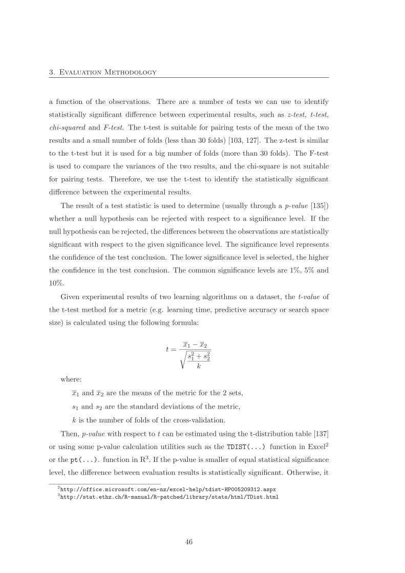
3. Evaluation Methodology
a function of the observations. There are a number of tests we can use to identify
statistically significant difference between experimental results, such as z-test, t-test,
chi-squared and F-test. The t-test is suitable for pairing tests of the mean of the two
results and a small number of folds (less than 30 folds) [103, 127]. The z-test is similar
to the t-test but it is used for a big number of folds (more than 30 folds). The F-test
is used to compare the variances of the two results, and the chi-square is not suitable
for pairing tests. Therefore, we use the t-test to identify the statistically significant
difference between the experimental results.
The result of a test statistic is used to determine (usually through a p-value [135])
whether a null hypothesis can be rejected with respect to a significance level. If the
null hypothesis can be rejected, the differences between the observations are statistically
significant with respect to the given significance level. The significance level represents
the confidence of the test conclusion. The lower significance level is selected, the higher
the confidence in the test conclusion. The common significance levels are 1%, 5% and
10%.
Given experimental results of two learning algorithms on a dataset, the t-value of
the t-test method for a metric (e.g. learning time, predictive accuracy or search space
size) is calculated using the following formula:
t =x1 − x2√s21 + s22
k
where:
x1 and x2 are the means of the metric for the 2 sets,
s1 and s2 are the standard deviations of the metric,
k is the number of folds of the cross-validation.
Then, p-value with respect to t can be estimated using the t-distribution table [137]
or using some p-value calculation utilities such as the TDIST(...) function in Excel2
or the pt(...). function in R3. If the p-value is smaller of equal statistical significance
level, the difference between evaluation results is statistically significant. Otherwise, it
2http://office.microsoft.com/en-nz/excel-help/tdist-HP005209312.aspx3http://stat.ethz.ch/R-manual/R-patched/library/stats/html/TDist.html
46

3. Evaluation Methodology
is not statistically significant.
Timeout for the learning algorithms (Q4)
A learning algorithm may not find a perfectly accurate definition. The basic reasons
are:
• The learning algorithm is not complete, i.e. it cannot produce some types of
concept, and the expected definition belongs to one of those types.
• The dataset contains noise and thus there is no accurate definition.
• There is not enough resource (e.g. memory) for the learning algorithm to find
the definition.
In this case, the learning algorithm will run out of memory before it produces and
returns the solution. As a result, some evaluation metrics cannot be computed.
Therefore, a maximal learning time, also called the timeout, for each learning algo-
rithm is assigned with respect to a dataset. If a learning algorithm reaches the maximal
learning time assigned before it produces an accurate solution, the algorithm will stop
and return the best solution it has produced so far (addressing Q4). The timeout value
assigned for an algorithm must ensure the learning algorithm stops and returns the
solution without running out of memory. In addition, it must not be too short to avoid
premature learning results.
To identify an appropriate timeout value for a learning algorithm with respect to a
dataset, we first run the learning algorithm on the dataset until it terminates. There
are two possible scenarios: i) the learning algorithm finds and returns a definition, and
ii) it runs out of memory without returning a definition. Figure 3.3 demonstrates the
above scenarios: the algorithm A can find a definition in around 10 minutes, whereas
the algorithm B runs out of memory after more than 50 minutes without getting an
accurate definition.
Based on the result of the investigation, the maximal learning time for a learning
algorithm is estimated as follows:
47
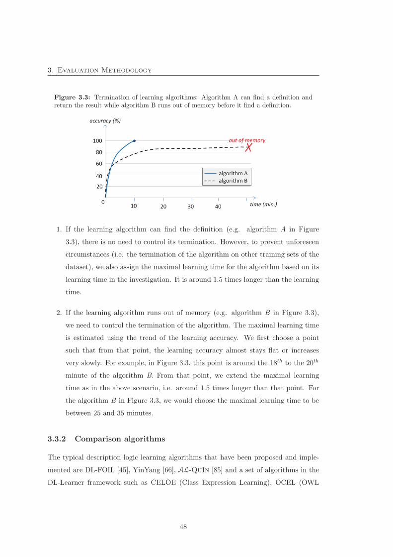
3. Evaluation Methodology
Figure 3.3: Termination of learning algorithms: Algorithm A can find a definition andreturn the result while algorithm B runs out of memory before it find a definition.
accuracy (%)
time (min.) 10 20 30 0
20
40
60
80
100
algorithm A algorithm B
out of memory
40
1. If the learning algorithm can find the definition (e.g. algorithm A in Figure
3.3), there is no need to control its termination. However, to prevent unforeseen
circumstances (i.e. the termination of the algorithm on other training sets of the
dataset), we also assign the maximal learning time for the algorithm based on its
learning time in the investigation. It is around 1.5 times longer than the learning
time.
2. If the learning algorithm runs out of memory (e.g. algorithm B in Figure 3.3),
we need to control the termination of the algorithm. The maximal learning time
is estimated using the trend of the learning accuracy. We first choose a point
such that from that point, the learning accuracy almost stays flat or increases
very slowly. For example, in Figure 3.3, this point is around the 18th to the 20th
minute of the algorithm B. From that point, we extend the maximal learning
time as in the above scenario, i.e. around 1.5 times longer than that point. For
the algorithm B in Figure 3.3, we would choose the maximal learning time to be
between 25 and 35 minutes.
3.3.2 Comparison algorithms
The typical description logic learning algorithms that have been proposed and imple-
mented are DL-FOIL [45], YinYang [66], AL-QuIn [85] and a set of algorithms in the
DL-Learner framework such as CELOE (Class Expression Learning), OCEL (OWL
48
3. Evaluation Methodology
Class Expression Learner) and ELTL (EL Tree Learner) [82]. Amongst the above
algorithms, we chose CELOE and OCEL to compare with our algorithms because:
1. They were well tested. Some detailed evaluations and comparisons were con-
ducted for these algorithms [57, 80]. They were compared with YinYang, ELTL,
Generic Programming (developed within DL-Learner), etc. The experimental re-
sults were also analysed and discussed using the basic metrics such as predictive
accuracy, learning time and definitions length. Therefore, it enables the implicit
comparison with other algorithms.
2. Evaluations in [57, 80] suggest that, overall, these algorithms produced better
results than other algorithms.
3. These algorithms and the DL-Learner framework are publicly available and they
can be accessed at the Sourceforge repository4. They also have a big user and
developer community.
4. They support expressive language. Although they were reported to support the
ALC language, the current implementation was extended to more expressive
power, e.g. at-least restriction and at-most restriction, and they approach the
support of the SHOIN(D) language.
In addition, these algorithms are the most recently developed description logic learn-
ing algorithms (in 2010). They were implemented in Java, a favourite platform used
best for web ontology language technologies and based on DL-Learner, an open source
framework for learning in description logics and OWL. The DL-Learner framework
provides core functionalities for implementation of description logic and OWL learn-
ing algorithms such as interfaces for different knowledge sources (e.g. OWL files and
SPARQL endpoints [29]), reasoner interfaces (e.g. OWLAPI reasoner interfaces and
DIG [10]), normalisation procedure, and implementation of some refinement operators.
Therefore, it allows direct comparisons by using the same methods for some parts (e.g.
refinement operator, reasoner interface and normalisation) of the implementation of
our learning algorithms. This helps to accomplish fair comparisons.
4http://dl-learner.svn.sourceforge.net/viewvc/dl-learner/
49
3. Evaluation Methodology
3.3.3 Evaluation Datasets
To ensure that our evaluations cover as much as possible of the space of cases, which
helps to achieve a thorough assessment of the algorithms involving in the evaluations,
we chose datasets that vary in: i) size, both for knowledge base and set of examples,
ii) the length of definitions, and iii) the noise property. In addition, datasets that
are commonly used in evaluations of symbolic machine learning may provide implicit
comparisons with other related approaches. Therefore, we also chose some datasets
commonly used in evaluation of symbolic learning algorithms, particularly in inductive
logic programming and description logic learning.
Based on the above criteria, we chose the following datasets for our evaluation.
The summary of their basic characters are given in Table 3.1 and their properties
are summarised in Table 3.2. In Table 3.1, we used CELOE, one of our comparison
algorithms, as the reference algorithm for estimation of the definition length of the
learning problems with respect to the datasets. We also assess the complexity of the
learning problems. The definition length is used as a proxy for the complexity.
However, this assessment may not be accurate if the dataset is noisy or the expected
definition for the learning problem with respect to the dataset is too long for CELOE
to produce the definition under an evaluation condition (e.g. memory). For example,
the average definition length for the CarcinoGenesis dataset produced by CELOE is 5
axioms. This is a short definition length and thus it is classified as a low complexity
learning problem. However, this is not a plausible classification as this is a noisy dataset
and the short definitions are caused by noisy data rather than a simple learning problem.
The average predictive accuracy of CELOE on this dataset is around 56%.
Moral
This dataset was first introduced in [140] and is available at the University of California
Irvine (UCI) machine learning repository5 [50]. This dataset contains concepts and
observations that are related to classification of activities as ‘guilty’ and ‘not guilty’.
It is intended to be used to learn definitions of harm-doing activities. This dataset
5http://archive.ics.uci.edu/ml/datasets/Moral+Reasoner
50

3. Evaluation Methodology
Table 3.1: Basic characters of the evaluation datasets. Some datasets includeseveral sub-datasets. Therefore, they may have more than one values for a charac-teristic.
No Dataset TBox sizea ABox sizeb Complexityc Noise
1. Moral Large Large Low No
2. Forte Uncle Small Small Medium No
3. Poker Medium Medium toLarge
Medium toHigh
No
4. Family Small Medium Low toVery high
No
5. CarcinoGenesis Large Large Low Yes
6. UCA1 (MUSE) Large Medium Medium No
7. ILPD Large Large Medium Yes
8. MUBus Medium Large Low toMedium
No
aTotal number of classes and properties. Small: (0, 8]; Medium: (8, 15]; Large: (15, ∞).bTotal number of assertions. Small: (0, 500]; Medium: (500, 1000]; Large: (1000, ∞)cThe complexity is approximately estimated based on the definition length. Low: (0, 8];
Medium: (8, 15]; High: (15, 20]; Very High: above 20.
includes two sub-datasets in which one of them requires a simple definition for harm-
doing activities, for example:
(blameworthy OR vicarious_blame)
Another one requires more complex definition for harm-doing activities, e.g.:
(NOT justified) AND (responsible OR vicarious)
Forte uncle
This is used to learn the definition of the concept Uncle. It was modified from the
Uncle dataset within the Family dataset by Lehmann [78]. A possible definition for
this learning problem is:
Male AND ((hasSibling SOME (hasChild some Person))
OR (married SOME (hasSibling SOME (hasChild SOME Person))))
51
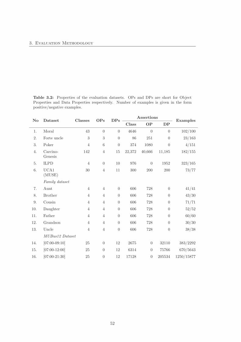
3. Evaluation Methodology
Table 3.2: Properties of the evaluation datasets. OPs and DPs are short for ObjectProperties and Data Properties respectively. Number of examples is given in the formpositive/negative examples.
No Dataset Classes OPs DPsAssertions
ExamplesClass OP DP
1. Moral 43 0 0 4646 0 0 102/100
2. Forte uncle 3 3 0 86 251 0 23/163
3. Poker 4 6 0 374 1080 0 4/151
4. Carcino-Genesis
142 4 15 22,372 40,666 11,185 182/155
5. ILPD 4 0 10 976 0 1952 323/165
6. UCA1(MUSE)
30 4 11 300 200 200 73/77
Family dataset
7. Aunt 4 4 0 606 728 0 41/41
8. Brother 4 4 0 606 728 0 43/30
9. Cousin 4 4 0 606 728 0 71/71
10. Daughter 4 4 0 606 728 0 52/52
11. Father 4 4 0 606 728 0 60/60
12. Grandson 4 4 0 606 728 0 30/30
13. Uncle 4 4 0 606 728 0 38/38
MUBus12 Dataset
14. [07:00-09:10] 25 0 12 2675 0 32110 383/2292
15. [07:00-12:00] 25 0 12 6314 0 75766 670/5643
16. [07:00-21:30] 25 0 12 17128 0 205534 1250/15877
52
3. Evaluation Methodology
This dataset is available at the DL-Leaner repository6.
Poker
This dataset contains description of poker hands. Each example in this dataset is a
description of a poker hand that consists of 5 cards drawn from a standard desk of
52 cards. Each card has two properties: suit and rank. There are four different suits:
Hearts, Spades, Diamonds and Clubs; and 13 different ranks: Ace, 2, 3, . . . , Queen,
King. There are totally 10 predictive attributes for a poker hand (i.e. suit of card 1,
rank of card 1, . . . , suit of card 5, rank of card 5).
A poker hand also has a Class attribute that describes its situation, e.g. one pair
(one pair of equal rank within five cards), two pairs (two pairs of equal rank within
five card), straight (five cards sequentially ranked with no gaps), etc. There are totally
10 poker hand classes. Therefore, this dataset can be used to learn the properties (or
the definitions) of poker hand classes. This dataset can be customised into binary-class
learning. It is available at the UCI repository7.
Family
This is a set of datasets that contains observations about the family relations such
as aunt, brother, cousin, daughter, father, grandson and uncle [113]. Therefore, there
are many learning problems in this dataset in which each of them is used to learn a
definition of a family relation. For example, the aunt relation is possibly defined as
follows:
Female AND ((hasSibling SOME hasChild SOME Thing) OR (married SOME
hasSibling SOME hasChild SOME Thing))
Or the definition of “Brother” relation, for instance, is as follows:
Male AND hasSibling SOME Thing
This dataset can be found in many repositories. In our evaluation, we use the
dataset distributed with the DL-Learner package (or can be found at the DL-Learner
6http://dl-learner.svn.sourceforge.net/viewvc/dl-learner/trunk/examples/forte/7http://archive.ics.uci.edu/ml/datasets/Poker+Hand
53
3. Evaluation Methodology
repository8).
CarcinoGenesis
This dataset is used to learn the structure of chemical compound and bio-essay that
may cause cancer. Data of this dataset was obtained from US National Toxicology
Program. It was transformed into logic programming and used for evaluation of ILP
algorithms by many authors such as in [7, 124]. This dataset was transformed into
OWL ontology format and used to evaluate the description logic learning algorithms
in the DL-Learner framework [80]. This is a challenging problem in machine learning
for both symbolic and sub-symbolic learning approaches, which is reported to contain
noise [80]. Therefore, this dataset is useful for testing the capability of dealing with
noise of the learning algorithms.
The OWL format of this dataset can be found in the DL-Learner distribution or
the DL-Learner repository9.
MUSE Dataset
This is a simulated smart home dataset created by the MUSE (Massey University Smart
Environment) research group [88] and available at the DL-Learner repository10. It is
simulated based on a set of use cases that particularly focus on describing normal and
abnormal behaviours of an inhabitant in a smart home. A major difference between this
dataset and other smart home datasets is that this dataset has richer context awareness
information. In most of the existing smart home datasets such as MIT [128], the only
context information involved is the time. However, the time data in that dataset is
only used to represent the order of the activities in the dataset. Other information of
the time data is not used such as the day of week and the season.
In the MUSE dataset, context awareness is taken into consideration. More infor-
mation is involved in the dataset than the existing home datasets such as seasons,
8http://dl-learner.svn.sourceforge.net/viewvc/dl-learner/trunk/examples/
family-benchmark/9http://dl-learner.svn.sourceforge.net/viewvc/dl-learner/trunk/examples/
carcinogenesis/10http://dl-learner.svn.sourceforge.net/viewvc/dl-learner/trunk/examples/
showering-duration/
54
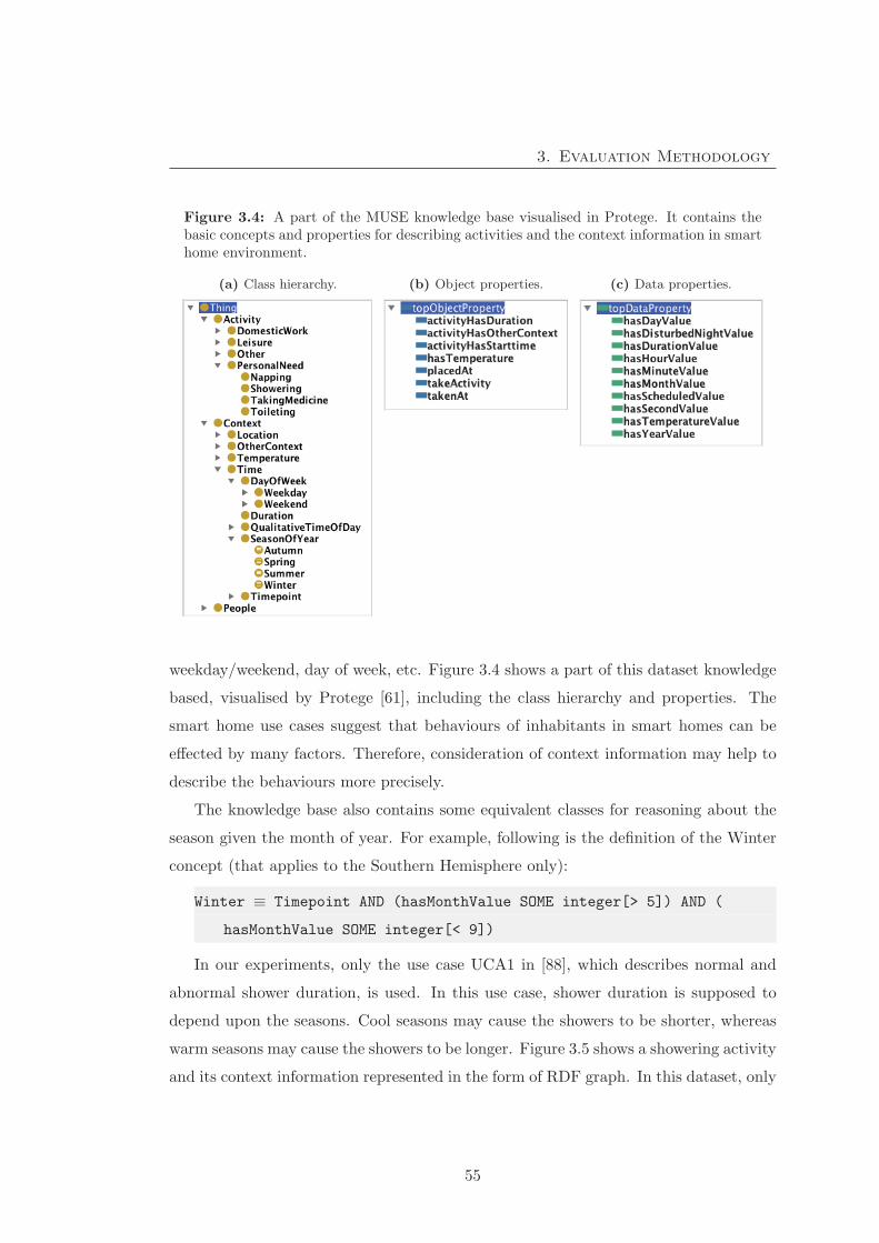
3. Evaluation Methodology
Figure 3.4: A part of the MUSE knowledge base visualised in Protege. It contains thebasic concepts and properties for describing activities and the context information in smarthome environment.
(a) Class hierarchy. (b) Object properties. (c) Data properties.
weekday/weekend, day of week, etc. Figure 3.4 shows a part of this dataset knowledge
based, visualised by Protege [61], including the class hierarchy and properties. The
smart home use cases suggest that behaviours of inhabitants in smart homes can be
effected by many factors. Therefore, consideration of context information may help to
describe the behaviours more precisely.
The knowledge base also contains some equivalent classes for reasoning about the
season given the month of year. For example, following is the definition of the Winter
concept (that applies to the Southern Hemisphere only):
Winter ≡ Timepoint AND (hasMonthValue SOME integer[> 5]) AND (
hasMonthValue SOME integer[< 9])
In our experiments, only the use case UCA1 in [88], which describes normal and
abnormal shower duration, is used. In this use case, shower duration is supposed to
depend upon the seasons. Cool seasons may cause the showers to be shorter, whereas
warm seasons may cause the showers to be longer. Figure 3.5 shows a showering activity
and its context information represented in the form of RDF graph. In this dataset, only
55

3. Evaluation Methodology
Figure 3.5: An example of a shower activity showering 001 in MUSE dataset and itscontext information represented in form of a RDF graph.
showering_001
6
Showering
rdf:type
timepoint_001
Timepoint
rdf:type
hasMonthValueduration_001
Duration
rdf:type
15
hasDurationValue
hasStarttimehasDuration
the month value of a timepoint is currently used. The month and duration values are
described by an integer value.
ILPD Dataset
This dataset contains liver function test records of patients collected from the North
East of Andhra Pradesh, India (Indian Liver Patient Dataset). Each record comprises
patient information such as age and gender and result of liver function tests including
total Bilirubin, direct Bilirubin, Albumin, total protein, Albumin/Globulin ratio, Ala-
nine, Aspartate and Alkaline Phosphatase. Based on the patient information and the
test results, experts were asked to classify patients’ record into cancer patient (denoted
by ‘1’) and non-cancer patient (denoted by ‘2’) classes. Therefore, this dataset can
be used to identify the characters of liver and non-liver cancer patient groups. This
dataset is also available in the UCI repository11.
The liver function test results are numeric values. In our evaluation, background
knowledge of liver function test is also included in the knowledge base of the learning
problem. This includes the definition of “normal” and “abnormal” value of the test
results based on reference range [52] collected and aggregated from several health labs
and website such as MedlinePlus12, a service of the US National Library of Medicine,
Virtual Medical Center13, a leading medical information website of Australia.
11http://archive.ics.uci.edu/ml/datasets/ILPD+(Indian+Liver+Patient+Dataset)12http://www.nlm.nih.gov/medlineplus/ency/article/003436.htm13http://www.virtualmedicalcentre.com/health-investigation/liver-function-tests-lfts
56
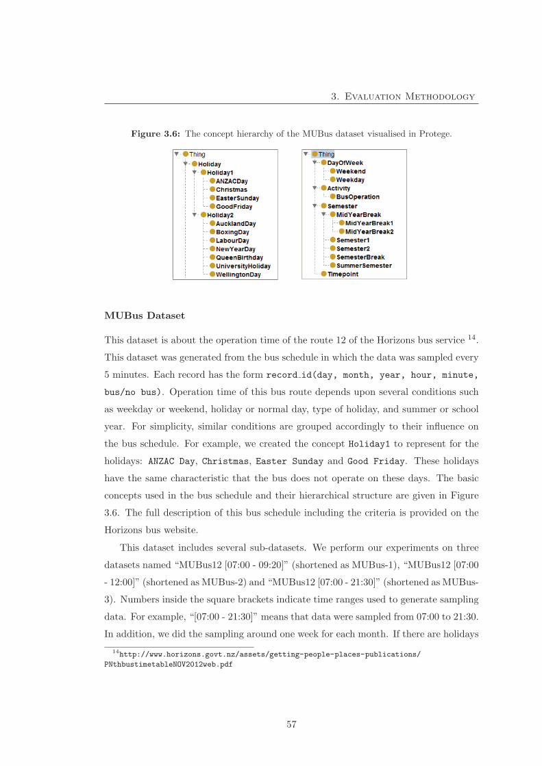
3. Evaluation Methodology
Figure 3.6: The concept hierarchy of the MUBus dataset visualised in Protege.
MUBus Dataset
This dataset is about the operation time of the route 12 of the Horizons bus service 14.
This dataset was generated from the bus schedule in which the data was sampled every
5 minutes. Each record has the form record id(day, month, year, hour, minute,
bus/no bus). Operation time of this bus route depends upon several conditions such
as weekday or weekend, holiday or normal day, type of holiday, and summer or school
year. For simplicity, similar conditions are grouped accordingly to their influence on
the bus schedule. For example, we created the concept Holiday1 to represent for the
holidays: ANZAC Day, Christmas, Easter Sunday and Good Friday. These holidays
have the same characteristic that the bus does not operate on these days. The basic
concepts used in the bus schedule and their hierarchical structure are given in Figure
3.6. The full description of this bus schedule including the criteria is provided on the
Horizons bus website.
This dataset includes several sub-datasets. We perform our experiments on three
datasets named “MUBus12 [07:00 - 09:20]” (shortened as MUBus-1), “MUBus12 [07:00
- 12:00]” (shortened as MUBus-2) and “MUBus12 [07:00 - 21:30]” (shortened as MUBus-
3). Numbers inside the square brackets indicate time ranges used to generate sampling
data. For example, “[07:00 - 21:30]” means that data were sampled from 07:00 to 21:30.
In addition, we did the sampling around one week for each month. If there are holidays
14http://www.horizons.govt.nz/assets/getting-people-places-publications/
PNthbustimetableNOV2012web.pdf
57
3. Evaluation Methodology
in a month, the sampling is extended to cover the holidays. This ensures the dataset
contains sufficient information for learning the patterns of bus operation time.
The learning problems with respect to this dataset are very complex learning prob-
lems. The bus operation schedule influences by many factors and thus the pattern to
describe the bus schedule is very long. For example, to describe only the bus schedule
in the weekend, the following description (or other equivalent descriptions) is required:
(NOT Holiday1) AND ((hasMinute VALUE 0 and hasHour VALUE 9) OR
(hasMinute VALUE 20 AND
(hasHour VALUE 10 OR hasHour VALUE 14 OR hasHour VALUE 16)) OR
(hasMinute VALUE 40 AND
(hasHour VALUE 11 OR hasHour VALUE 13 OR hasHour VALUE 15)))
Or the criteria of the bus depart at 09:20 is as follows:
(hasHour VALUE 9 AND hasMinute VALUE 20) AND
Weekday AND (NOT Holiday1) AND (NOT MidYearBreak2) AND
(NOT MidYearBreak1) AND (NOT SemesterBreak) AND (NOT SummerSemester)
The full description of the bus schedule is very complex. Therefore, this dataset is
used to assess the ability of the learning algorithms in handling the complex learning
problems. This dataset is also suitable for evaluating the symmetric learning approach
as the negative examples in this dataset can be described by simple description, e.g.
NOT Holiday1. This dataset is available at the DL-Learner repository15.
3.4 Implementation and Running the Code
Our algorithms have been implemented in Java programming language. This is the
favourite platform used best for web ontology language technologies such as OWL
application programming interface (OWLAPI [11]) and OWL reasoners (e.g. Pellet
[107], Hermit [117] and FaCT [63]). Therefore, using this platform will facilitate our
implementation and also help our work to be as close as possible to others.
Our evaluation is implemented and available online 16. Scripts for reproducing
15http://dl-learner.svn.sourceforge.net/viewvc/dl-learner/trunk/examples/16https://parcel-2013.googlecode.com/files/parcel-cli.zip
58
3. Evaluation Methodology
the experimental results are also included in this package. A detailed description of
the evaluation system configuration and instructions for running evaluation scripts are
provided in Appendix B.
Note that different evaluation system configurations may produce different experi-
mental results for some particular metrics. Learning time is the most sensitive metric to
the evaluation system configuration. Other metrics such as learnt concept, search space
size and accuracy are less dependent on the system configuration than learning time
and thus the evaluation usually produces the similar results for these metrics regardless
of the evaluation system.
59

3. Evaluation Methodology
60

Chapter 4
Adaptive Numerical Data
Segmentation
This chapter describes an approach to segmentation of numeric data property
values that will be useful in the rest of the thesis. We first present the standard
approach to refinement of numeric data properties in description logic learning
and discuss its limitations. Then, we propose an approach to segmentation
of numeric data property values. Finally, we present experimental results to
demonstrate the effectiveness of our approach.
4.1 Introduction
Refinement of a description is done by: i) adding (specialisation) or removing (gen-
eralisation) primitive concepts, roles and restrictions to/from the description, and ii)
refining the primitive concepts, roles and restrictions in the description. The refine-
ment of a primitive concept, role and restriction are based on a quasi-order space that
consists of a set of values and a quasi-ordering [104]. They are basically a replacement
of the concept, role or restriction by a more specific (downward refinement) or a more
general (upward refinement) element in the quasi-order set.
The quasi-order space for primitive concept refinement consists of the set of prim-
itive concepts in the TBox (NC) and the sub-concept relation ( ). Similarly, the
61
4. Adaptive Numerical Data Segmentation
quasi-order space for role refinement consists of primitive roles in the TBox (NR) and
the sub-role relation ( ). Identifying quasi-order sets for primitive concepts and roles
are straight forward, as all required information is available within the knowledge base.
However, a quasi-order set for refinement of restrictions is not always available, par-
ticularly for numeric datatypes. The quasi-ordering for numbers is obviously available.
For examples, we can use >,≥, <, or ≤ to define the generality and specificity be-
tween the numeric values. On the other hand, the set of elements of the quasi-order set
for numeric datatype restriction refinement is not explicitly available in the knowledge
base. A computation is often needed to identify this set.
In this chapter, a method for identifying the elements of the quasi-order set for
refinement for numeric datatype properties is proposed. This is a pre-processing step,
that only has to be done once, before the learning starts. This method will be used by
all the learning algorithms developed in this thesis. To demonstrate the efficacy of the
method, we will present experimental results of this method implemented in CELOE
and one of our algorithms, the ParCEL algorithm, developed in Chapter 5.
4.2 Motivation
Learning symbolic concepts is the ultimate purpose of the symbolic learning approach.
Therefore, most existing approaches in description logic learning focus upon learning
symbolic concepts without appropriate attention to learning numeric datatypes. How-
ever, in many real-world applications, numeric data has an important role in knowledge
representation and it cannot always be replaced by qualitative representations, i.e sym-
bolic concepts.
In existing description logic learning approaches, the most common method for re-
fining numeric datatype properties is to use the maximal (≤) and minimal (≥) value
restriction (quasi-orderings) on a set of values, which are usually obtained from the
range values of the datatype properties’ assertions. Figure 4.1 visualises the speciali-
sation process for a numeric datatype property p. Specialisation in Figure 4.1(a) uses
either the maximal or minimal value restriction and the specialisation in Figure 4.1(b)
uses both of them. With n possible values for refinement for a datatype property p,
62

4. Adaptive Numerical Data Segmentation
Figure 4.1: Specialisation of numeric datatype properties.
(a) Either maximal or minimal value restriction is used by the specialisation.
(b) Both maximal and minimal value restrictions are used by the specialisation.
1 2 3 4 5 6 . . . n-2 n-1 n Property p
1 p n p (n-1)
2 p n
specialisation specialisation
there are 2n possible combinations for one-sided specialisation and n(n+1)2 combinations
for two-sided specialisation of p, as illustrated in Figures 4.1(a) and 4.1(b) respectively.
To the best of our knowledge, amongst description logic learning algorithms devel-
oped, the only description logic learning algorithms that explicitly describe and imple-
ment the specification of the numeric datatype property refinement are the CELOE,
OCEL and ELTL algorithms in the DL-Learner framework [82]. As the number of
assertions of a datatype property may be very big, using all the values of the assertions
may explode the search space due to the number of possible combinations. Therefore,
in these algorithms, a fixed-size segmentation method is used to reduce the refinement
space. In this method, a maximal number of values for refining a numeric datatype
property is assigned. If k is the maximal number of values used for the refinement of a
datatype property, the assertion values of the datatype property are split into k equal
parts and the middle values of split parts are used for refinement (they are rounded for
the integer datatype). Figure 4.2 describes a segmentation for a data property p that
63
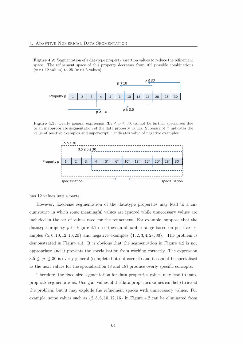
4. Adaptive Numerical Data Segmentation
Figure 4.2: Segmentation of a datatype property assertion values to reduce the refinementspace. The refinement space of this property decreases from 102 possible combinations(w.r.t 12 values) to 25 (w.r.t 5 values).
p ≥ 1.0 p ≥ 3.5
p ≤ 18 p ≤ 30
. . .
. . .
Property p
Figure 4.3: Overly general expression, 3.5 ≤ p ≤ 30, cannot be further specialised dueto an inappropriate segmentation of the data property values. Superscript + indicates thevalue of positive examples and superscript − indicates value of negative examples.
1 2 3 4 5+ 6+ 10+ 12+ 16+ 20+ 28 30
1
3.5
Property p
specialisation specialisation
has 12 values into 4 parts.
However, fixed-size segmentation of the datatype properties may lead to a cir-
cumstance in which some meaningful values are ignored while unnecessary values are
included in the set of values used for the refinement. For example, suppose that the
datatype property p in Figure 4.2 describes an allowable range based on positive ex-
amples {5, 6, 10, 12, 16, 20} and negative examples {1, 2, 3, 4, 28, 30}. The problem is
demonstrated in Figure 4.3. It is obvious that the segmentation in Figure 4.2 is not
appropriate and it prevents the specialisation from working correctly. The expression
3.5 ≤ p ≤ 30 is overly general (complete but not correct) and it cannot be specialised
as the next values for the specialisation (8 and 18) produce overly specific concepts.
Therefore, the fixed-size segmentation for data properties values may lead to inap-
propriate segmentations. Using all values of the data properties values can help to avoid
the problem, but it may explode the refinement spaces with unnecessary values. For
example, some values such as {2, 3, 6, 10, 12, 16} in Figure 4.2 can be eliminated from
64
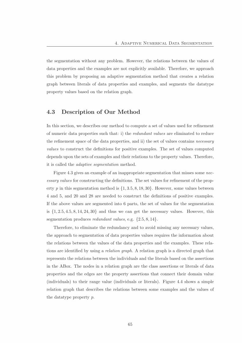
4. Adaptive Numerical Data Segmentation
the segmentation without any problem. However, the relations between the values of
data properties and the examples are not explicitly available. Therefore, we approach
this problem by proposing an adaptive segmentation method that creates a relation
graph between literals of data properties and examples, and segments the datatype
property values based on the relation graph.
4.3 Description of Our Method
In this section, we describes our method to compute a set of values used for refinement
of numeric data properties such that: i) the redundant values are eliminated to reduce
the refinement space of the data properties, and ii) the set of values contains necessary
values to construct the definitions for positive examples. The set of values computed
depends upon the sets of examples and their relations to the property values. Therefore,
it is called the adaptive segmentation method.
Figure 4.3 gives an example of an inappropriate segmentation that misses some nec-
essary values for constructing the definitions. The set values for refinement of the prop-
erty p in this segmentation method is {1, 3.5, 8, 18, 30}. However, some values between
4 and 5, and 20 and 28 are needed to construct the definitions of positive examples.
If the above values are segmented into 6 parts, the set of values for the segmentation
is {1, 2.5, 4.5, 8, 14, 24, 30} and thus we can get the necessary values. However, this
segmentation produces redundant values, e.g. {2.5, 8, 14}.Therefore, to eliminate the redundancy and to avoid missing any necessary values,
the approach to segmentation of data properties values requires the information about
the relations between the values of the data properties and the examples. These rela-
tions are identified by using a relation graph. A relation graph is a directed graph that
represents the relations between the individuals and the literals based on the assertions
in the ABox. The nodes in a relation graph are the class assertions or literals of data
properties and the edges are the property assertions that connect their domain value
(individuals) to their range value (individuals or literals). Figure 4.4 shows a simple
relation graph that describes the relations between some examples and the values of
the datatype property p.
65
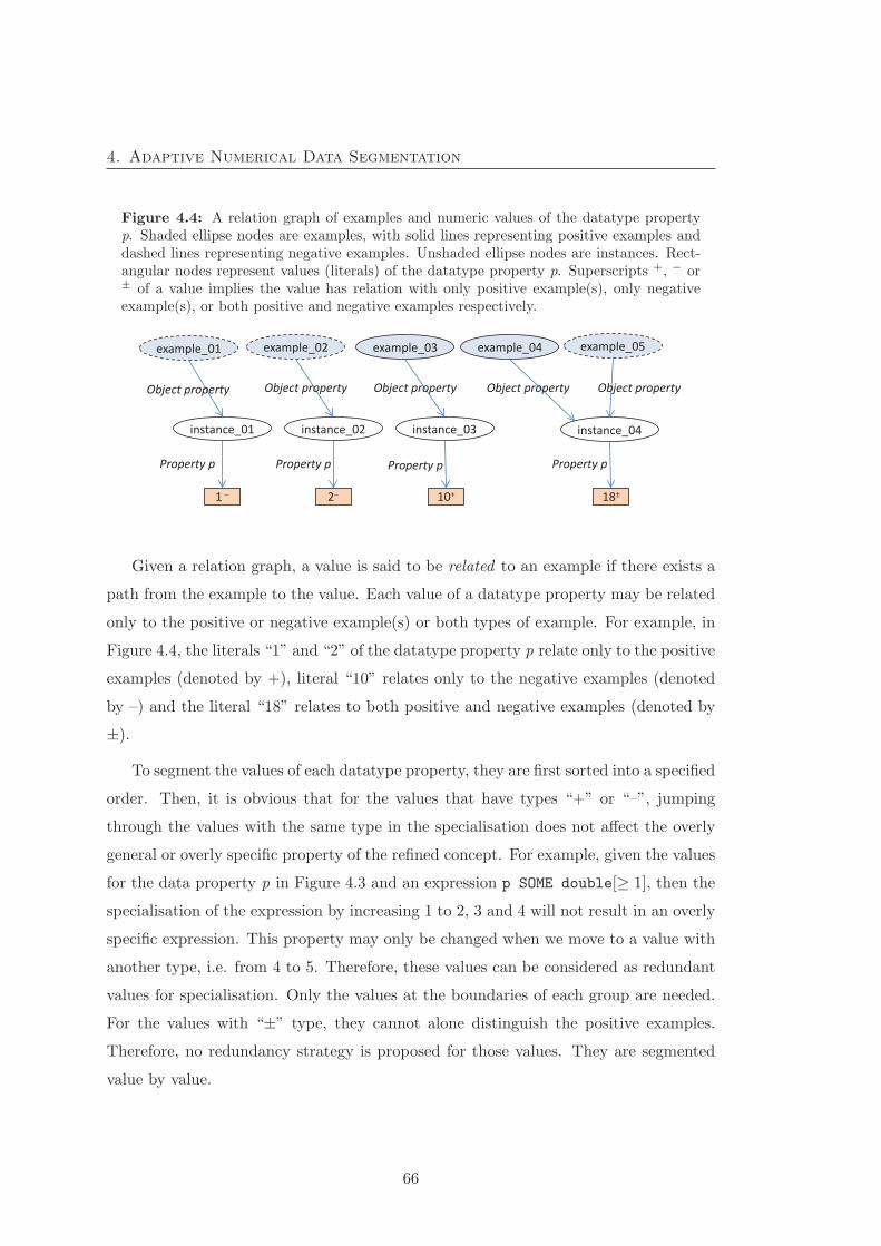
4. Adaptive Numerical Data Segmentation
Figure 4.4: A relation graph of examples and numeric values of the datatype propertyp. Shaded ellipse nodes are examples, with solid lines representing positive examples anddashed lines representing negative examples. Unshaded ellipse nodes are instances. Rect-angular nodes represent values (literals) of the datatype property p. Superscripts +, − or± of a value implies the value has relation with only positive example(s), only negativeexample(s), or both positive and negative examples respectively.
instance_01 instance_02 instance_03
example_01
1 2 10+
instance_04
18±
example_02 example_03 example_04 example_05
Property p
Object property
Property p Property p Property p
Object property Object property Object property Object property
Given a relation graph, a value is said to be related to an example if there exists a
path from the example to the value. Each value of a datatype property may be related
only to the positive or negative example(s) or both types of example. For example, in
Figure 4.4, the literals “1” and “2” of the datatype property p relate only to the positive
examples (denoted by +), literal “10” relates only to the negative examples (denoted
by –) and the literal “18” relates to both positive and negative examples (denoted by
±).
To segment the values of each datatype property, they are first sorted into a specified
order. Then, it is obvious that for the values that have types “+” or “–”, jumping
through the values with the same type in the specialisation does not affect the overly
general or overly specific property of the refined concept. For example, given the values
for the data property p in Figure 4.3 and an expression p SOME double[≥ 1], then the
specialisation of the expression by increasing 1 to 2, 3 and 4 will not result in an overly
specific expression. This property may only be changed when we move to a value with
another type, i.e. from 4 to 5. Therefore, these values can be considered as redundant
values for specialisation. Only the values at the boundaries of each group are needed.
For the values with “±” type, they cannot alone distinguish the positive examples.
Therefore, no redundancy strategy is proposed for those values. They are segmented
value by value.
66

4. Adaptive Numerical Data Segmentation
Figure 4.5: Segmentation of data property values. Values are sorted and then groupedby type. There are 6 segments from s1 to s6 and 7 values are computed for specialisation.
v1 v2 v3 v4+ v5
+ v6+ v7
+ v8± v9
± v10+ v11 v12
v13
s1 s2 s3 s4 s5 s6
Values
Segments
Values for spec. (v3 + v4)/2 (v7 + v8)/2 (v8 + v9)/2
(v9+ v10)/2 (v11+ v12)/2
Figure 4.6: Applying our segmentation method for segmenting the values in Figure4.3 and computing the values for the specification. There are 3 segments and 4 valuescomputed.
1 2 3 4 5+ 6+ 10+ 12+ 16+ 20+ 28 30 Values
Segments
Values for spec.
s1 s2 s3
4.5 24
Finally, the set of values used for the specialisation of each data property is com-
puted from the values at the boundary of the segments. They may be the average of
the two values at the boundary. Rounding may be needed for integer datatype prop-
erties. Figure 4.5 demonstrates a segmentation and the computation of the values for
specialisation with 7 values are computed for the specialisation. Figure 4.6 shows gives
a particular example for segmenting the values in Figure 4.3. There are 3 segments and
only 4 values are computed for the specialisation.
A disadvantage of this strategy in comparison with the fixed-size segmentation
strategy is that it requires an extra computational cost for building the relation graph.
4.4 The Algorithms
Our datatype property values segmentation aims to reduce redundancy and avoid miss-
ing any necessary values in the refinement of numeric data properties. Our approach
is based on the directed graph that represents relation between examples and values
of the numeric data properties. Therefore, the first step in our algorithm is to build a
relation graph. Then, we check if a value is connected with positive or negative exam-
ples or both of them. Finally, the values of numeric data properties using the above
information are segmented.
The algorithm for building relation graphs is given in Algorithm 4.1. Each edge v
67
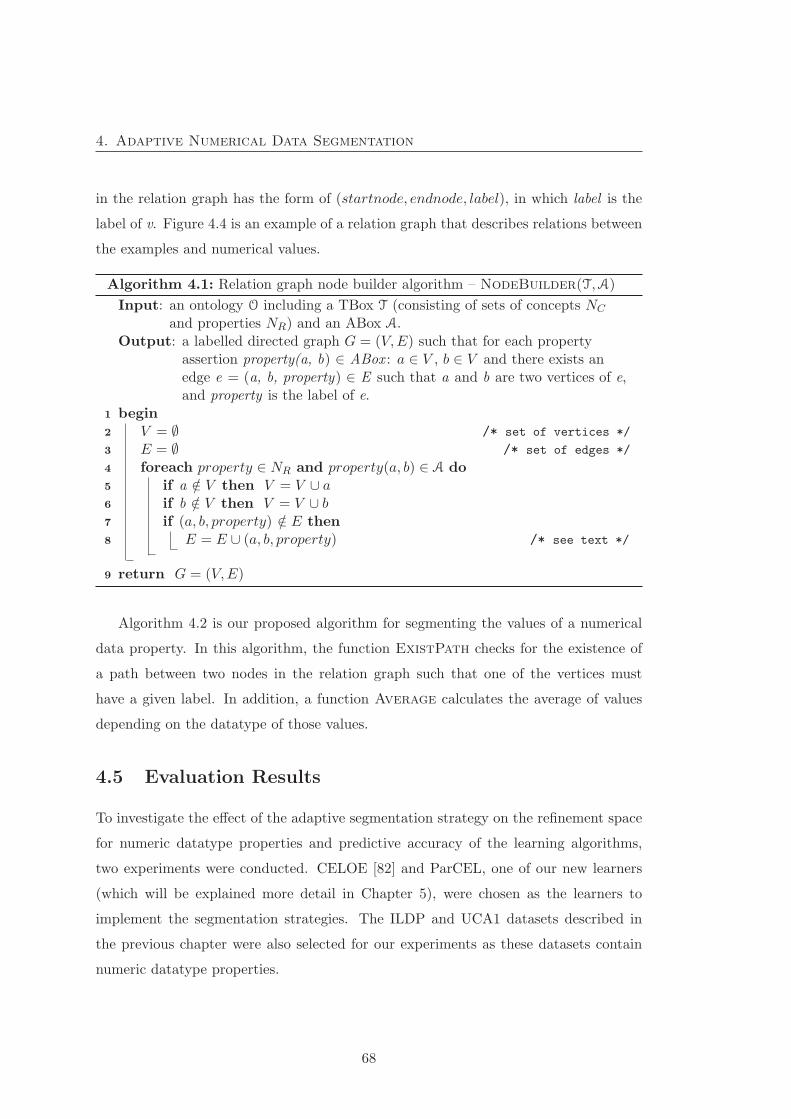
4. Adaptive Numerical Data Segmentation
in the relation graph has the form of (startnode, endnode, label), in which label is the
label of v. Figure 4.4 is an example of a relation graph that describes relations between
the examples and numerical values.
Algorithm 4.1: Relation graph node builder algorithm – NodeBuilder(T,A)
Input: an ontology O including a TBox T (consisting of sets of concepts NC
and properties NR) and an ABox A.Output: a labelled directed graph G = (V,E) such that for each property
assertion property(a, b) ∈ ABox : a ∈ V , b ∈ V and there exists anedge e = (a, b, property) ∈ E such that a and b are two vertices of e,and property is the label of e.
1 begin2 V = ∅ /* set of vertices */
3 E = ∅ /* set of edges */
4 foreach property ∈ NR and property(a, b) ∈ A do5 if a /∈ V then V = V ∪ a6 if b /∈ V then V = V ∪ b7 if (a, b, property) /∈ E then8 E = E ∪ (a, b, property) /* see text */
9 return G = (V,E)
Algorithm 4.2 is our proposed algorithm for segmenting the values of a numerical
data property. In this algorithm, the function ExistPath checks for the existence of
a path between two nodes in the relation graph such that one of the vertices must
have a given label. In addition, a function Average calculates the average of values
depending on the datatype of those values.
4.5 Evaluation Results
To investigate the effect of the adaptive segmentation strategy on the refinement space
for numeric datatype properties and predictive accuracy of the learning algorithms,
two experiments were conducted. CELOE [82] and ParCEL, one of our new learners
(which will be explained more detail in Chapter 5), were chosen as the learners to
implement the segmentation strategies. The ILDP and UCA1 datasets described in
the previous chapter were also selected for our experiments as these datasets contain
numeric datatype properties.
68
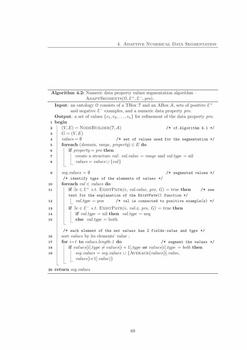
4. Adaptive Numerical Data Segmentation
Algorithm 4.2: Numeric data property values segmentation algorithm –AdaptSegments(O,E+,E−, pro).
Input: an ontology O consists of a TBox T and an ABox A, sets of positive E+
and negative E− examples, and a numeric data property pro.Output: a set of values {v1, v2, . . . , vn} for refinement of the data property pro.
1 begin2 (V,E) = NodeBuilder(T,A) /* cf.Algorithm 4.1 */
3 G = (V,E)4 values = ∅ /* set of values used for the segmentation */
5 foreach (domain, range, property) ∈ E do6 if property = pro then7 create a structure val : val.value = range and val.type = nil8 values = values ∪ {val}
9 seg values = ∅ /* segmented values */
/* identify type of the elements of values */
10 foreach val ∈ values do11 if ∃e ∈ E+ s.t. ExistPath(e, val.value, pro, G) = true then /* see
text for the explanation of the ExistPath() function */
12 val.type = pos /* val is connected to positive example(s) */
13 if ∃e ∈ E− s.t. ExistPath(e, val.x, pro, G) = true then14 if val.type = nil then val.type = neg15 else val.type = both
/* each element of the set values has 2 fields:value and type */
16 sort values by its elements’ value ;17 for i=1 to values.length-1 do /* segment the values */
18 if values[i].type �= values[i+ 1].type or values[i].type = both then19 seg values = seg values ∪ {Average(values [i].value,
values [i+1].value)}
20 return seg values
69
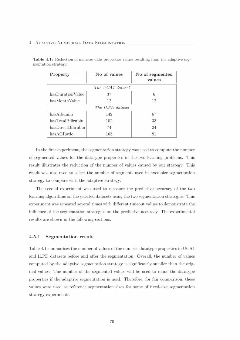
4. Adaptive Numerical Data Segmentation
Table 4.1: Reduction of numeric data properties values resulting from the adaptive seg-mentation strategy.
Property No of values No of segmentedvalues
The UCA1 dataset
hasDurationValue 37 6
hasMonthValue 12 12
The ILPD dataset
hasAlbumin 142 67
hasTotalBilirubin 102 33
hasDirectBilirubin 74 24
hasAGRatio 163 81
In the first experiment, the segmentation strategy was used to compute the number
of segmented values for the datatype properties in the two learning problems. This
result illustrates the reduction of the number of values caused by our strategy. This
result was also used to select the number of segments used in fixed-size segmentation
strategy to compare with the adaptive strategy.
The second experiment was used to measure the predictive accuracy of the two
learning algorithms on the selected datasets using the two segmentation strategies. This
experiment was repeated several times with different timeout values to demonstrate the
influence of the segmentation strategies on the predictive accuracy. The experimental
results are shown in the following sections.
4.5.1 Segmentation result
Table 4.1 summarises the number of values of the numeric datatype properties in UCA1
and ILPD datasets before and after the segmentation. Overall, the number of values
computed by the adaptive segmentation strategy is significantly smaller than the orig-
inal values. The number of the segmented values will be used to refine the datatype
properties if the adaptive segmentation is used. Therefore, for fair comparison, these
values were used as reference segmentation sizes for some of fixed-size segmentation
strategy experiments.
70
4. Adaptive Numerical Data Segmentation
4.5.2 Experimental results on the accuracy
In this experiment, the predictive accuracy of CELOE and ParCEL on the two datasets
were measured using both the fixed-size and adaptive segmentation methods. There-
fore, there are 4 experimental results reported in this section.
The experimental result on the IDLP dataset
CELOE over-fits on the ILDP datasets: the higher the training accuracy, the lower
the predictive accuracy. Therefore, the training accuracy is needed to demonstrate the
effect of the segmentation on learning results.
In CELOE, a number of segmentations are used for all datatype properties, i.e.
different numbers of segmentations for each property cannot be selected. Therefore, the
number of segmentations used in this experiment was selected based on: i) the default
number of segmentations used by CELOE (10 segments), ii) the minimal number of
segmented values computed by the adaptive segmentation (24) for the given dataset
(see Table 4.1), iii) the maximal number of segmented values computed by the adaptive
segmentation (81), and iv) the maximal number of values of all properties (163). The
experimental result of CELOE on the ILDP datasets is shown in Table 4.2.
Both CELOE and ParCEL were first used to learn this problem but both these al-
gorithms could not find solutions in more than 10 minutes. Therefore, several timeouts
for the experiment were assigned: 60s, 90s, 120s and 180s. The experimental results
show that CELOE always got highest training accuracy with the adaptive segmentation
strategy for each timeout value. The accuracy of the fixed-size segmentation with 10
segments at 108s is still lower than that of the adaptive strategy at 60s. The highest
accuracy of the largest segmentation (i.e. segment size 163) is equal to that of the
adaptive strategy at 60s. Further investigation with the largest segmentations shown
that this strategy was able to achieve the same accuracy with that of the adaptive
strategy at 120s, at 600s. This is attributed by the bigger search space of the (largest)
fixed-size segmentation in comparison with the adaptive segmentation.
Therefore, it can be concluded that the adaptive segmentation can help the learning
to achieve higher accuracy faster than the fixed-size segmentation. In addition, it can
avoid the inappropriate segmentation problem found by the fixed-size strategy.
71
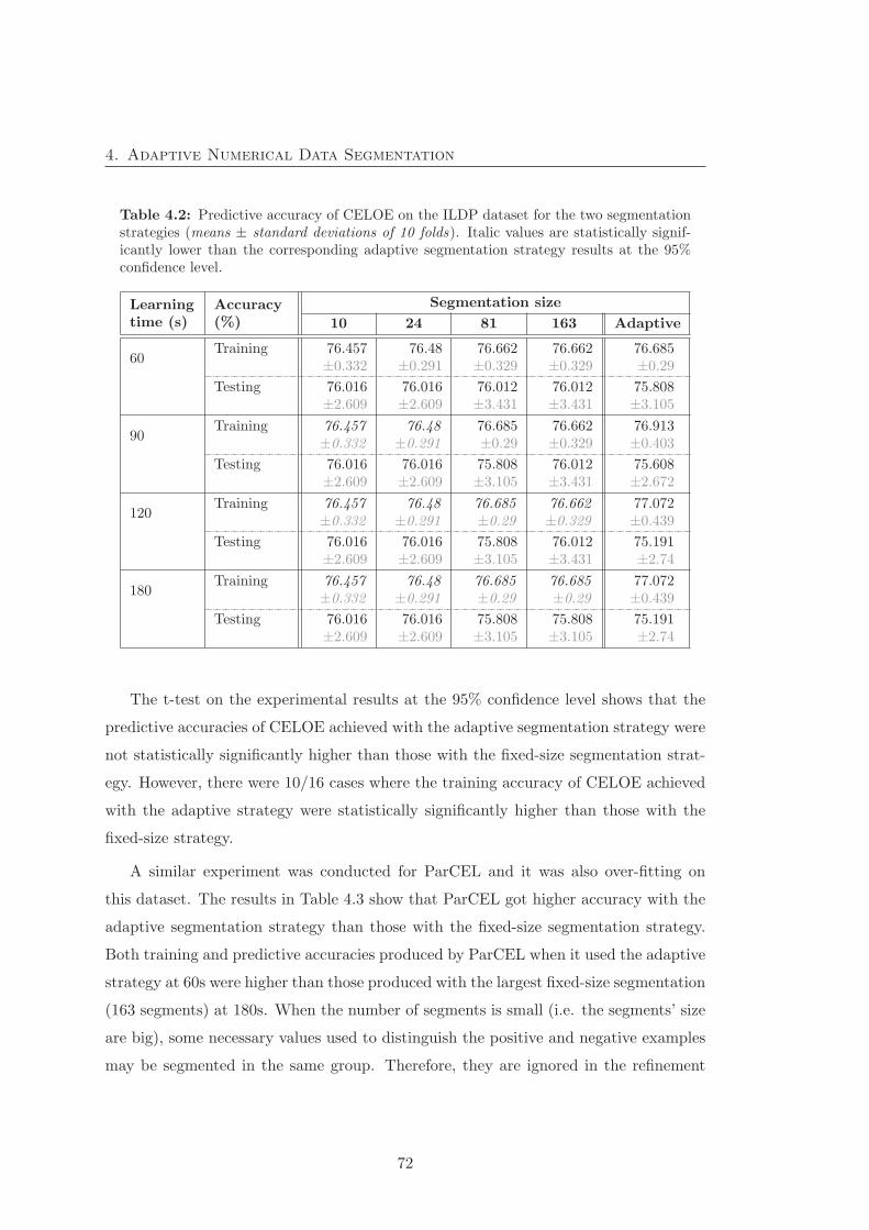
4. Adaptive Numerical Data Segmentation
Table 4.2: Predictive accuracy of CELOE on the ILDP dataset for the two segmentationstrategies (means ± standard deviations of 10 folds). Italic values are statistically signif-icantly lower than the corresponding adaptive segmentation strategy results at the 95%confidence level.
Learningtime (s)
Accuracy(%)
Segmentation size
10 24 81 163 Adaptive
60Training 76.457
±0.33276.48
±0.29176.662±0.329
76.662±0.329
76.685±0.29
Testing 76.016±2.609
76.016±2.609
76.012±3.431
76.012±3.431
75.808±3.105
90Training 76.457
±0.33276.48
±0.29176.685±0.29
76.662±0.329
76.913±0.403
Testing 76.016±2.609
76.016±2.609
75.808±3.105
76.012±3.431
75.608±2.672
120Training 76.457
±0.33276.48
±0.29176.685±0.29
76.662±0.329
77.072±0.439
Testing 76.016±2.609
76.016±2.609
75.808±3.105
76.012±3.431
75.191±2.74
180Training 76.457
±0.33276.48
±0.29176.685±0.29
76.685±0.29
77.072±0.439
Testing 76.016±2.609
76.016±2.609
75.808±3.105
75.808±3.105
75.191±2.74
The t-test on the experimental results at the 95% confidence level shows that the
predictive accuracies of CELOE achieved with the adaptive segmentation strategy were
not statistically significantly higher than those with the fixed-size segmentation strat-
egy. However, there were 10/16 cases where the training accuracy of CELOE achieved
with the adaptive strategy were statistically significantly higher than those with the
fixed-size strategy.
A similar experiment was conducted for ParCEL and it was also over-fitting on
this dataset. The results in Table 4.3 show that ParCEL got higher accuracy with the
adaptive segmentation strategy than those with the fixed-size segmentation strategy.
Both training and predictive accuracies produced by ParCEL when it used the adaptive
strategy at 60s were higher than those produced with the largest fixed-size segmentation
(163 segments) at 180s. When the number of segments is small (i.e. the segments’ size
are big), some necessary values used to distinguish the positive and negative examples
may be segmented in the same group. Therefore, they are ignored in the refinement
72

4. Adaptive Numerical Data Segmentation
Table 4.3: Predictive accuracy of ParCEL on the ILDP dataset for the two segmentationstrategies (means ± standard deviations of 10 folds). The statistical significance test resultsare presented using the same conventions as in Table 4.2.
Learningtime (s)
Accuracy(%)
Segmentation size
10 24 81 163 Adaptive
60Training 58.583
±1.67966.984±1.391
75.954±1.799
77.138±1.761
83.628±1.369
Testing 54.278±9.907
62.477±7.818
64.068±8.608
64.472±8.906
68.567±7.413
90Training 58.583
±1.67966.984±1.391
78.892±1.555
77.867±1.378
84.971±1.349
Testing 54.278±9.907
62.477±7.818
65.709±7.633
64.472±8.906
69.804±6.923
120Training 58.583
±1.67966.984±1.391
79.689±1.553
78.391±1.595
85.404±1.184
Testing 54.074±9.768
62.477±7.818
67.359±7.214
65.493±8.25
70.004±7.482
180Training 58.583
±1.67966.984±1.391
80.736±1.538
82.466±1.489
85.632±1.178
Testing 54.074±9.768
62.477±7.818
67.997±7.349
67.967±6.559
70.629±7.031
that resulted in the low learning accuracy. The learning accuracy of the fixed-size
segmentation strategy was also lower than the adaptive segmentation even when the
number of segmentations was set to the maximal numbers of possibles values in the
domain. This can also be attributed to the bigger search space of this strategy in
comparison with the adaptive segmentation strategy.
The t-test on the training and predictive accuracies at 95% confidence shows that
the training accuracies of the adaptive segmentation strategy on UCA1 dataset were
statistically significantly higher than those of the fixed-size strategy for all segment
sizes and learning times. On the other hand, the predictive accuracies of the adaptive
strategy were statistically significantly higher than the fixed-size strategy when the
segment sizes are 10 and 24.
The experimental result on the UCA1 dataset
The number of segments used for the fixed-size segmentation strategy was selected
similarly for the UCA1 dataset. Both CELOE and ParCEL were not over-fitting on
73
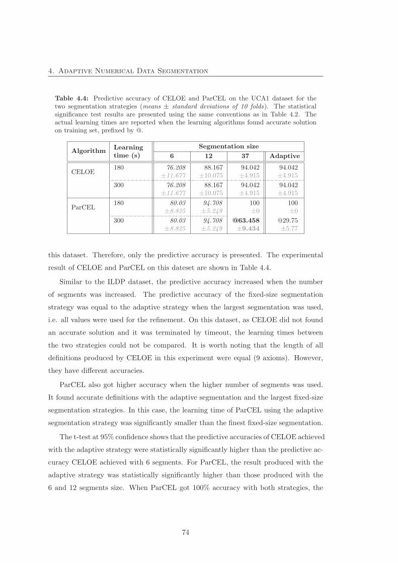
4. Adaptive Numerical Data Segmentation
Table 4.4: Predictive accuracy of CELOE and ParCEL on the UCA1 dataset for thetwo segmentation strategies (means ± standard deviations of 10 folds). The statisticalsignificance test results are presented using the same conventions as in Table 4.2. Theactual learning times are reported when the learning algorithms found accurate solutionon training set, prefixed by @.
AlgorithmLearningtime (s)
Segmentation size
6 12 37 Adaptive
CELOE180 76.208
±11.67788.167
±10.07594.042±4.915
94.042±4.915
300 76.208±11.677
88.167±10.075
94.042±4.915
94.042±4.915
ParCEL180 80.03
±8.82594.708±5.249
100±0
100±0
300 80.03±8.825
94.708±5.249
@63.458±9.434
@29.75±5.77
this dataset. Therefore, only the predictive accuracy is presented. The experimental
result of CELOE and ParCEL on this dateset are shown in Table 4.4.
Similar to the ILDP dataset, the predictive accuracy increased when the number
of segments was increased. The predictive accuracy of the fixed-size segmentation
strategy was equal to the adaptive strategy when the largest segmentation was used,
i.e. all values were used for the refinement. On this dataset, as CELOE did not found
an accurate solution and it was terminated by timeout, the learning times between
the two strategies could not be compared. It is worth noting that the length of all
definitions produced by CELOE in this experiment were equal (9 axioms). However,
they have different accuracies.
ParCEL also got higher accuracy when the higher number of segments was used.
It found accurate definitions with the adaptive segmentation and the largest fixed-size
segmentation strategies. In this case, the learning time of ParCEL using the adaptive
segmentation strategy was significantly smaller than the finest fixed-size segmentation.
The t-test at 95% confidence shows that the predictive accuracies of CELOE achieved
with the adaptive strategy were statistically significantly higher than the predictive ac-
curacy CELOE achieved with 6 segments. For ParCEL, the result produced with the
adaptive strategy was statistically significantly higher than those produced with the
6 and 12 segments size. When ParCEL got 100% accuracy with both strategies, the
74
4. Adaptive Numerical Data Segmentation
learning time with the adaptive strategy was statistically significantly smaller than
those resulted by the largest fixed-size segmentation strategy.
4.6 Conclusion
The approach to segmentation of the numeric data property produced promising results.
It helped to reduce the number of values used in refinement of numeric data properties
significantly. More importantly, the experimental results showed that decrease of the
refinement values did not lessen the predictive accuracy. Moreover, it increased the
predictive accuracy for some learning problems by avoid missing of any necessary values
in the refinements.
75

4. Adaptive Numerical Data Segmentation
76
Chapter 5
Parallel Class Expression
Learning
This chapter proposes a Parallel Class Expression Learning approach to learn-
ing Web Ontology Language (OWL) class expressions. We first describe the
class learning problem and some existing approaches in the literature. Then,
we present an approach to class expression learning that combines the top-
down approach with a reduction strategy, and uses parallelisation to improve
the learning speed. Finally, evaluations of our proposed approach, together
with comparisons with other algorithms, are presented.
5.1 Parallelisation for Class Expression Learning
Parallelisation is a popular technique to speed up the processing of an application. It
has been used in many application domains, particularly following the introduction
of multi-core processors, as are currently used in most computer systems. In logic
programming, this technique is used to create parallel logic programming or parallel
inference algorithms such as [28, 53, 84, 129]. In inductive logic programming, the
root of description logic learning, some parallel inductive logic learning algorithms
have also been proposed [37, 49, 93, 106]. However, in description logics, particularly
77
5. Parallel Class Expression Learning
in Web Ontology Language, parallelisation is being mainly used only in the OWL
inference algorithms [122]. In description logic learning, to the best of our knowledge,
there is no parallel description logic learner. Therefore, the main objective of this
chapter is to propose a Parallel Class Expression Learning algorithm that employs
parallelisation to utilise the power of multi-core computers or that can be developed
for cloud computing platforms such as Amazon EC2. The name Class Expression
Learning is used instead of Description Logic Learning to focus on the Web Ontology
Language (OWL) representation languages, related techniques and applications.
Class expression learning
As defined in Definition 2.16, the description logic learning problem is to find a concept
(class expression) that covers a set of examples. Given a knowledge base K and sets of
positive E+ and negative E− examples such that E+∩E− = ∅, description logic learning
aims to find a class expression C such that K |= C(e) for all e ∈ E+ and K � C(e) for
all e ∈ E−.
There are two basic approaches to class expression logic learning. The top-down
approach is preferred as it can utilise the sub-concept (subclass) semantics provided
within the knowledge base for performing specialisation in its downward refinement
operator [6, 43, 66]. Most existing description logic learning algorithms use this ap-
proach, as reported in the literature, such as [43, 45, 66, 85]. On the other hand, the
bottom-up approach cannot inherit the concept hierarchy structure of the knowledge
base. The upward refinement operators used in this approach mainly use the most
specific concepts (MSC) calculation based on the set of positive examples [31, 72]. The
most specific concept of an individual is the most specific class expression such that
the individual is an instance of that expression.
Empirically, the top-down learning algorithms tend to produce short and readable
definitions. Contrarily, bottom-up learning algorithms tend to generate (unnecessarily)
long concepts. In addition, MSC have only been used with FL and FLE languages [39].
MSC for more expressive languages have not yet been investigated and hence they can
only be approximated [3, 34, 75]. Therefore, the top-down approach is preferred to the
bottom-up approach in description logic learning. However, this approach does not suit
78
5. Parallel Class Expression Learning
well for learning long definitions.
A combination of the top-down and bottom-up approaches was proposed in DL-
FOIL [45]. In this approach, top-down (specialisation) is the main task in the learning
process to find definitions for positive examples and disjunction is used to generalise
the set of definitions. A combination of downward refinement and the MSC operator
for specialisation and disjunction for generalisation is introduced in YinYang [66]. A
major advantage of this approach over the top-down approach is that it can deal well
with complex learning problems, i.e. learning problems that need a long definition.
However, the experimental results show that YinYang still produces unnecessarily long
concepts [80]. Similarly, the current greedy partial solutions disjunction strategy of
DL-FOIL is not an optimal strategy for short definitions.
Amongst the existing class expression learning approaches, the combination of the
top-down and bottom-up approaches is the most suitable for parallelisation as the par-
tial solutions can be learnt simultaneously. Therefore, a three-step class expression
learning approach, which is based on the above approach, is proposed to benefit par-
allelisation for class expression learning and address the problem of unnecessarily long
learnt definitions. In this approach, the generalisation is separated from the speciali-
sation by a reduction step. It allows the creation of the final definition according to
the specific requirements, such as short final definition and small number of definitions
involved in the final definition.
5.2 Description of Our Method
In this section, a Parallel Class Expression Learning algorithm (ParCEL) is proposed
that combines both the top-down and bottom-up approaches to handle learning prob-
lems that require long definitions. In addition, a reduction operation between the
top-down and bottom-up steps is also introduced to reduce the definition length. This
operation can be customised to achieve other criteria instead of short definition length
such as a smaller number of partial definitions (see Definition 5.2).
The learning process is separated into three steps: specialisation, reduction and
generalisation (aggregation). First, the specialisation is used to generate correct, but
79
5. Parallel Class Expression Learning
not necessarily complete, class expressions (i.e. each expression must cover some posi-
tive examples and no negative ones). Then, the class expressions produced in the first
step are reduced to select the best candidates for building the final definition. Finally,
the best candidates are aggregated to form the final definition. In this approach, the
aggregation simply creates the disjunction of the best candidates.
Before describing the approach in detail, we introduce some related concepts.
Definition 5.1 (Irrelevant concept). Given a description logic learning problem
LP = 〈K, (E+,E−)〉 as defined in Definition 2.16, a concept C is called irrelevant if
K � C(e) for all e ∈ E+, i.e. it covers none of the positive examples. �
Definition 5.2 (Partial definition). Given a learning problem LP = 〈K, (E+,E−)〉,a concept is called a partial definition if it is correct (i.e. covers no negative example)
and not irrelevant (covers some positive examples) with respect to LP. It is also called
the definition of the covered positive examples. �
Therefore, the first step of the approach aims to find partial definitions for the
positive examples. Formally, given a learning problem LP = 〈K, (E+,E−)〉, this step is
to find a set of partial definitions P such that⋃
pi∈P cover(K, pi,E+) = E+. The finding
of partial definitions uses the top-down approach, which starts from the most general
concept TOP. Then, the downward refinement operator proposed by Lehmann et al.
[82] is adopted to specialise the concepts until all positive examples are covered by the
partial definitions. Figure 5.1 demonstrates the specialisation process. The expressions
are organised as a tree of expressions called the search tree. The children of a node are
the refinement result of their parent node. Therefore, the learning problem is a search
for partial definitions in a search tree.
The downward refinement operator used in CELOE [82] is modified to make it
suitable for our approach. The top-down step of our algorithm aims to find the partial
definitions instead of a complete definition. In addition, since the disjunction is used
in the generalisation step to combine the partial definitions, it is not necessary to
use disjunction in the top-down step. The downward refinement operator used in our
approach can now be defined:
Definition 5.3 (ParCEL downward refinement operator ρ¬�). Given an expres-
80
5. Parallel Class Expression Learning
Figure 5.1: The specialisation process. ρ is a downward refinement operator. Ci are classexpressions. The children of a node are the refinement results of that node.
(TOP)
(C1)
TOP
C1 C3 C4
C11 C12 C41
(C4)
C2
sion C, a set of concept names NC and a set of property (role) names NR in which NRO
is a set of object properties and NRD is a set of data properties, then ρ¬� is defined as
follows:
1. if C ∈ NC (C is an atomic concept):
ρ¬�(C) = {C ′ | C ′ � C and �C ′′ ∈ NC : C ′ � C ′′ � C} ∪ {C � C ′ | C ′ ∈ ρ¬�()}(if C is an atomic concept, it is specialised by using its proper sub-concepts or
creating a conjunction with the refinements of the TOP concept).
2. if C = (C is the TOP concept):
ρ¬�(C) = {C ′ | C ′ ∈ NC , �C ′′ ∈ NC : C ′ � C ′′ � C}∪ {¬C ′ | C ′ ∈ NC , �C ′′ ∈ NC : C ′′ � C ′}∪ {∃r. | r ∈ NRO} ∪ {∀r. | r ∈ NRO}∪ {∃r.V | r ∈ NRD, V ∈ mgdr(r)} ∪ {∀r.V | r ∈ NRD, V ∈ mgdr(r)}
(if C is the TOP concept, specialise it by using its proper sub-concepts or property
restrictions)
3. if C = ¬D,D ∈ NC (C is a negation of an atomic concept):
ρ¬�(C) = {¬D′ | D � D′ and �D′′ : D � D′′ � D′} ∪ {C � C ′ | C ′ ∈ ρ¬�()}(if C is a negation of a concept, specialise it by the upward refinement of the
negated concept)
4. if (C = C1 � ... � Cn (C is a conjunctive of descriptions):
ρ¬�(C) = {C ′ | C ′ ∈ ρ¬�(Ci), 1 ≤ i ≤ n}(if C is a conjunction, it is specialised by refinements of its conjuncts)
81
5. Parallel Class Expression Learning
5. if C = ∀r.D, r ∈ NRO: ρ¬�(C) = {∀r.D′ | D′ ∈ ρ�(D)}
(if C is a ‘for all’ object property restriction, it is specialised by refinements of its
range)
6. if C = ∃r.D, r ∈ NRO: ρ¬�(C) = {∃r.D′ | D′ ∈ ρ¬�(D)}
(this rule is for the ‘exists’ object property restriction, similar to the 5th rule.)
7. if C = ∀r.V, r ∈ NRD: ρ¬�(C) = {∀r.V ′ | V ′ = next(r, V )}
(if C is ‘for all’ datatype property restriction, it is specialised by using the next
value in its segments (see Section 4.3))
8. if C = ∃r.V, r ∈ NRD: ρ¬�(C) = {∃r.V ′ | V ′ = next(r, V )}
(similar to the 7th rule, applied for ‘exists’ datatype property restriction) �
where mgdr(r) is the most general data range value for the property r and next(r,
V ) is the next value of V in r. Here, the scope of the refinement is restricted to the
numeric data properties and they are defined as:
mgdr(r) = {≥ min(AdaptSegments(r)),≤ max(AdaptSegments(r))}
next(r, V ) =
⎧⎪⎪⎪⎪⎪⎨⎪⎪⎪⎪⎪⎩
≥ u′ | u′ ∈ AdaptSegments(r) and u′ > u and
�u′′ ∈ AdaptSegments(r) : u′ > u′′ > u, if V ∈ ≥ u
≤ u′ | u′ ∈ AdaptSegments(r) and u′ < u and
�u′′ ∈ AdaptSegments(r) : u′ < u′′ < u, if V ∈ ≤ u
where AdaptSegments(r) is the set of segmented values for the property r. A method
for computation of this set is described in Section 4.3 and Algorithm 4.2.
The selection of nodes (expressions) in the search tree is controlled by the score
of the nodes that are calculated by a search heuristic. In addition, parallelisation is
employed to find the partial definitions in parallel. In particular, multiple branches
within the tree can be traversed by multiple workers to find the partial definitions.
A central reducer monitors the finding of the partial definitions of the workers until
the partial definitions cover all positive examples. Then, it aggregates the partial
definitions to the overall definition. The reducer also has the responsibility of removing
redundant partial definitions that cover overlapping sets of positive examples. The
parallel exploration of the search tree by two workers is demonstrated in Figure 5.2.
82
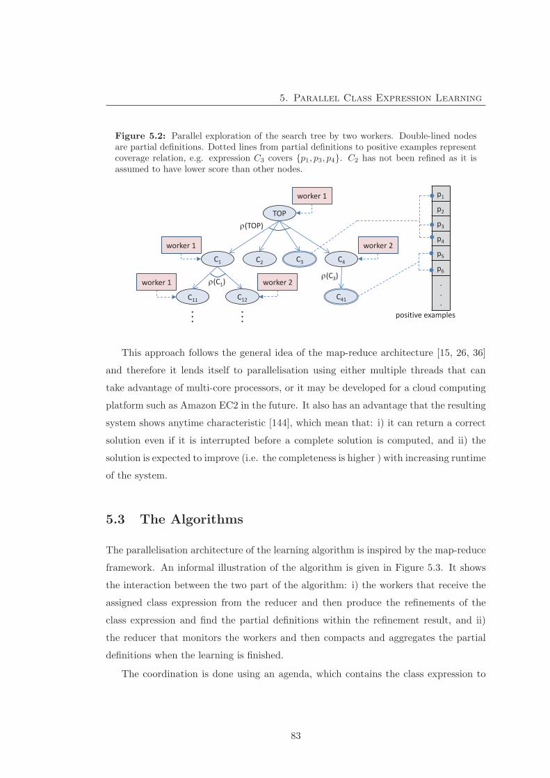
5. Parallel Class Expression Learning
Figure 5.2: Parallel exploration of the search tree by two workers. Double-lined nodesare partial definitions. Dotted lines from partial definitions to positive examples representcoverage relation, e.g. expression C3 covers {p1, p3, p4}. C2 has not been refined as it isassumed to have lower score than other nodes.
(TOP)
(C1)
TOP
C1 C4
C11 C12
(C3)
worker 1
worker 1
worker 1 worker 2
p1
p2
p3
p4
p5
p6
.
.
.
worker 2
C3
. . .
. . . C41
C2
positive examples
This approach follows the general idea of the map-reduce architecture [15, 26, 36]
and therefore it lends itself to parallelisation using either multiple threads that can
take advantage of multi-core processors, or it may be developed for a cloud computing
platform such as Amazon EC2 in the future. It also has an advantage that the resulting
system shows anytime characteristic [144], which mean that: i) it can return a correct
solution even if it is interrupted before a complete solution is computed, and ii) the
solution is expected to improve (i.e. the completeness is higher ) with increasing runtime
of the system.
5.3 The Algorithms
The parallelisation architecture of the learning algorithm is inspired by the map-reduce
framework. An informal illustration of the algorithm is given in Figure 5.3. It shows
the interaction between the two part of the algorithm: i) the workers that receive the
assigned class expression from the reducer and then produce the refinements of the
class expression and find the partial definitions within the refinement result, and ii)
the reducer that monitors the workers and then compacts and aggregates the partial
definitions when the learning is finished.
The coordination is done using an agenda, which contains the class expression to
83
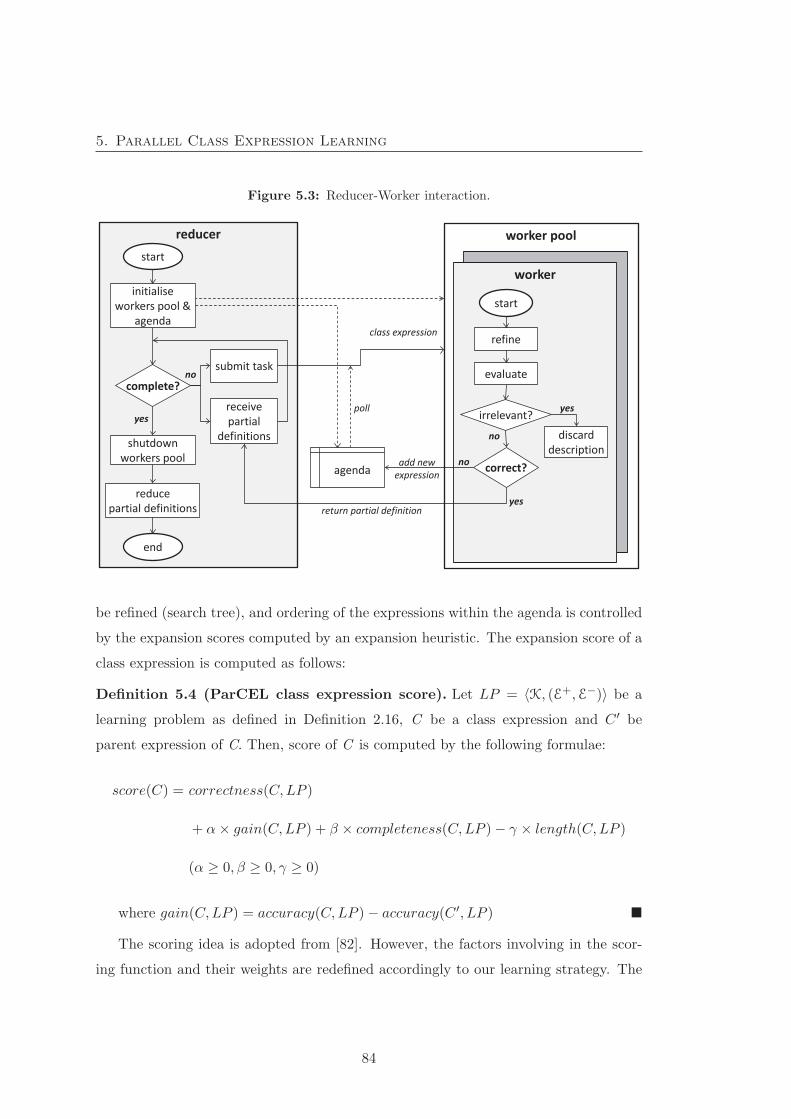
5. Parallel Class Expression Learning
Figure 5.3: Reducer-Worker interaction.
worker pool reducer start
worker
start
refine
submit task
receive partial
definitions
complete?
shutdown workers pool
reduce partial definitions
evaluate
irrelevant?
correct? agenda
end
poll
no
discard description
yes
add new expression
no
yes
return partial definition yes
no
class expression
initialise workers pool &
agenda
be refined (search tree), and ordering of the expressions within the agenda is controlled
by the expansion scores computed by an expansion heuristic. The expansion score of a
class expression is computed as follows:
Definition 5.4 (ParCEL class expression score). Let LP = 〈K, (E+,E−)〉 be a
learning problem as defined in Definition 2.16, C be a class expression and C ′ be
parent expression of C. Then, score of C is computed by the following formulae:
score(C) = correctness(C,LP )
+ α× gain(C,LP ) + β × completeness(C,LP )− γ × length(C,LP )
(α ≥ 0, β ≥ 0, γ ≥ 0)
where gain(C,LP ) = accuracy(C,LP )− accuracy(C ′, LP ) �
The scoring idea is adopted from [82]. However, the factors involving in the scor-
ing function and their weights are redefined accordingly to our learning strategy. The
84
5. Parallel Class Expression Learning
heuristic is mainly based on correctness of the class expression ([82] is based on ac-
curacy). Then, a penalty is applied for long definitions to avoid infinite deep search
because the refinement operator used in our learning algorithm is infinite. On the other
hand, a level of bonus for accuracy gained by an expression is also applied. The intu-
ition behind the bonus for accuracy gained by expressions is that those expressions are
more likely to be close to the solution. In addition, a bonus is given for the completeness
of expressions.
We chose α = 0.2, β = 0.01, γ = 0.05. The choice of these values is based on experi-
mental investigations in [82]. These values can be adjusted based on the characteristics
of the learning problem. For instance, we can decrease the penalty level for learning
problems that have been reported to have long definitions so that the search will give
bias towards deep search.
Our algorithm can now be defined in two parts. The computationally heavy part
is done by the multiple workers : this is the refinement and the evaluation of class
expressions. In particular, the evaluation of (complex) concepts (i.e. checking whether
a given example is an instance of a concept) requires an ontology reasoner. By default,
Pellet [107] is used for this purpose.
The reducer creates a worker pool, which manages a number of workers, assigns new
tasks (class expressions for refinement and evaluation) to the worker pool, and updates
the agenda and the set of cumulative partial definitions based on the refinement result
returned from workers until the completeness of the combined partial definitions is
sufficient. Then the reducer tries to reduce the number of partial definitions in order to
remove redundancies using a reduction function Reduce (see Algorithm 5.3). While
the reducer computes sets of concepts, these sets can be easily aggregated into a single
concept using disjunction. Before introducing the complete learning problem, a function
cover to compute a set of instances covered by a set of class expressions is introduced
as below.
Definition 5.5 (Cover function). Given a knowledge base K, a set of individuals E
and a set of class expressions X, then function cover is defined as follows:
cover(K,X,E) = {e ∈ E | ∃C ∈ X such that K |= C(e)} �
85

5. Parallel Class Expression Learning
The complete algorithm of the Reducer is given in Algorithm 5.1.
Algorithm 5.1: Reducer Algorithm
Input: a learning problem LP = 〈K, (E+,E−)〉 as defined in Definition 2.16, anda noise value ε ∈ [0, 1] (0 means no noise).
Output: a set of partial definitions X s.t. |cover(K,X,E+)| ≥ (|E+| × (1− ε))and cover(K,X,E−) = ∅ (empty set).
1 begin2 initialise an agenda = {} /* : the TOP concept */
3 cum pdefs = ∅ /* cumulative partial definitions */
4 cum upos = E+ /* cumulative uncovered positive examples */
5 initialise a worker pool
6 while |cum upos| > (|E+| × ε) do7 execute the following tasks in parallel:
8 begin [task: submit tasks to the worker pool ]9 if worker pool is not full then
10 select the highest score expression C in agenda11 submit new task (C,E+,E−) to worker pool
12 begin [task: receive result from workers]13 wait for sets of (expressions, pdefs) from workers14 agenda = agenda ∪ expressions15 cum pdefs = cum pdefs ∪ pdefs
/* remove positive examples covered by pdefs from cum upos */
16 cum upos = cum upos \ cover(K, pdefs, E+)
17 return Reduce(cum pdefs) /* cf. Algorithm 5.3 */
The worker algorithm refines an expression and evaluates the refinement results. It
will first check whether concepts are irrelevant. If this is the case, the concepts can be
safely removed from the computation as no partial definition can be computed through
specialisation. If an expression is a partial definition (i.e., correct and not irrelevant),
it is added to the partial definitions set. If a concept is not irrelevant, but also not
correct (i.e., if it covers some positive and some negative examples), it is added to the
set of new expressions. Then, the worker returns these sets back to the reducer. The
complete algorithm for workers is defined in Algorithm 5.2.
Note that the concepts that have been refined can be scheduled for further refine-
86
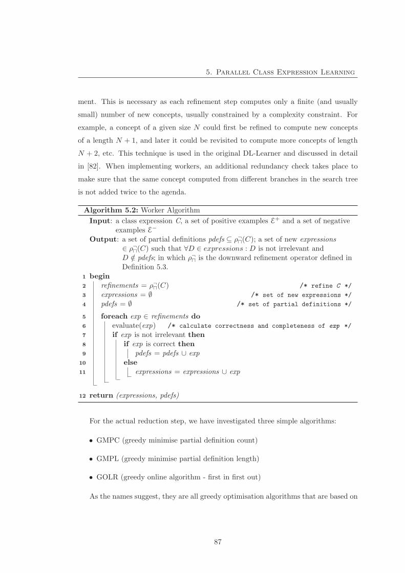
5. Parallel Class Expression Learning
ment. This is necessary as each refinement step computes only a finite (and usually
small) number of new concepts, usually constrained by a complexity constraint. For
example, a concept of a given size N could first be refined to compute new concepts
of a length N + 1, and later it could be revisited to compute more concepts of length
N + 2, etc. This technique is used in the original DL-Learner and discussed in detail
in [82]. When implementing workers, an additional redundancy check takes place to
make sure that the same concept computed from different branches in the search tree
is not added twice to the agenda.
Algorithm 5.2: Worker Algorithm
Input: a class expression C, a set of positive examples E+ and a set of negativeexamples E−
Output: a set of partial definitions pdefs ⊆ ρ¬�(C); a set of new expressions∈ ρ¬�(C) such that ∀D ∈ expressions : D is not irrelevant andD /∈ pdefs; in which ρ¬� is the downward refinement operator defined inDefinition 5.3.
1 begin2 refinements = ρ¬�(C) /* refine C */
3 expressions = ∅ /* set of new expressions */
4 pdefs = ∅ /* set of partial definitions */
5 foreach exp ∈ refinements do6 evaluate(exp) /* calculate correctness and completeness of exp */
7 if exp is not irrelevant then8 if exp is correct then9 pdefs = pdefs ∪ exp
10 else11 expressions = expressions ∪ exp
12 return (expressions, pdefs)
For the actual reduction step, we have investigated three simple algorithms:
• GMPC (greedy minimise partial definition count)
• GMPL (greedy minimise partial definition length)
• GOLR (greedy online algorithm - first in first out)
As the names suggest, they are all greedy optimisation algorithms that are based on
87
5. Parallel Class Expression Learning
sorting the partial definitions. Once the partial definitions are sorted, a new solution
set (called the reduction set) is created and solutions are added to this set in descending
order. A definition is added only if it covers at least one positive example not yet covered
by any other solution in the reduction set. A formal generic reduction algorithm based
on a sort function is defined in Algorithm 5.3.
Different sort criteria have been used, resulting in the different algorithms. In
GMPC, partial definitions are sorted according to the number of positive examples
they cover, preferring definitions that cover more positive examples. If two definitions
cover the same number of positive examples, the lexicographical order of the respective
string representations is used as a tiebreaker. This is important to make the results
repeatable. Otherwise, the order that is used when iterating over definitions could
depend on internal system hash codes, which the application does not control.
In GMPL, definitions are sorted according to their expression lengths, preferring
definitions with a shorter length. If two definitions have the same expression length,
we again use the lexicographical order.
In GOLR, we use time stamps assigned to definitions when they are added to the
solutions, preferring definitions that were added earlier. While the other two heuristics
have to be run in batch mode after a complete set of definitions has been computed, this
algorithm can be employed just-in-time: the reduction can take place whenever a new
definition is found and added. This algorithm is therefore very space efficient compared
to the other two. On the other hand, how timestamps are assigned in an application
may depend on thread scheduling. This again cannot be controlled completely by the
application, causing variations in the results between runs.
5.4 Evaluation Result
To evaluate the proposed algorithms, three experiments were conducted using the eval-
uation methodology described in Chapter 3. For the experiments, we used a Linux
server with a 2 x Intel Quad-core Xeon E5440 @2.83GHz processor, 32GB memory
and the Redhat 4.1.2 (Linux version 2.6.18) operating system with a JRE 1.6.0 (64-bit)
Java Virtual Machine (JVM). The default heap size of the JMV in our experiments was
88

5. Parallel Class Expression Learning
Algorithm 5.3: Generic greedy reduction algorithm based on sorting
Input: a set of class expression D, a Sort function that provides a strategy forsorting a set of class expressions, and a learning problem 〈K, (E+,E−)〉.
Output: a set of class expressions D′ ⊆ D such that⋃d∈D cover(K, d,E+) =
⋃d∈D′ cover(K, d,E+) = E+, in which function
cover is defied in Definition 3.1.1 begin2 D′ = ∅ (empty set)3 cpos = ∅ /* covered positive examples */
4 while D is not empty and cpos ⊂ E+ do5 Sort(D) /* sort class expressions in D */
6 d = poll(D) /* remove and assign the top element in D to d */
7 if cover(K, d,E+) � cpos then8 D′ = D′ ∪ d9 cpos = cpos ∪ cover(K, d,E+)
10 return D′
8GB. The computer used in the experiments has 8 cores. The number of workers used
for ParCEL is 6 workers as we wanted to reserve 1 core for the learner (main thread)
and 1 core for the system tasks.
The first experiment aims to investigate the predictive accuracy and learning time
of our learning algorithm and compare the experimental results with CELOE, our
selected comparison algorithm (Section 5.4.1). The second experiment observes the
affect of parallelisation on the learning process (Section 5.4.2). The third experiment is
to demonstrate the effect of the reduction strategy on the length of the learnt definitions
(Section 5.4.3).
5.4.1 Experiment 1 - Comparison between ParCEL and CELOE
In this experiment, both CELOE and ParCEL were executed on the same system for
the selected datasets and the predictive accuracy, learning time and description length
produced by these algorithms on each dataset were then measured. Timeouts were
also assigned for these algorithms based on the strategy described in Chapter 3. The
length of definition reported is the length of the best expression learnt so far. Table
5.1 shows a summary of the experimental results. In this table, the definition length of
89

5. Parallel Class Expression Learning
ParCEL is reported by the number of partial definitions and the average length of the
partial definitions. Therefore, the average length of ParCEL definitions are the product
of those numbers. The reduction mechanism used in our experiments is GMPC (see
Section 5.2).
Table 5.1: Experiment result summary (means ± standard deviations of 10 folds). Boldvalues are statistically significantly better than the unformatted values in the statisticalsignificance test at the 95% confidence level. There was no significance test for the definitionlength.
Problem Learning time (s) Accuracy (%)(Avg. partial)∗
def. lengthNo. of
partial
def.
CELOE ParCEL CELOE ParCEL CELOE ParCEL ParCEL
Moral 0.15
±0.03
0.02
±0.01
100.00
±0.00
100.00
±0.00
3.00
±0.00
1.52
±0.05
2.10
±0.32
Forte 2.60
±1.64
0.23
±0.17
98.86
±2.27
100.00
±0.00
13.50
±1.00
7.75
±0.05
2.00
±0.00
Poker-
Straight
0.36
±0.71
0.59
±0.08
100.00
±0.00
96.43
±4.12
11.70
±0.68
10.90
±1.31
1.70
±0.68
Aunt 30.01
±0.02
0.26
±0.15
96.5
±0.00
100.00
±0.00
19.00
±0.00
8.80
±0.48
2.00
±0.00
Brother 0.19
±0.16
0.03
±0.02
100.00
±0.00
100.00
±0.00
6.00
±0.00
6.00
±1.83
1.00
±0.00
Cousin 3.79
±0.54
0.54
±0.20
99.29
±0.00
99.29
±2.26
23.40
±2.59
8.50
±0.00
2.00
±0.00
Daughter 0.2
±0.02
0.03
±0.03
100.00
±0.00
100.00
±0.00
5.00
±0.00
5.25
±1.09
1.10
±0.32
Father 0.02
±0.10
0.03
±0.03
100.00
±0.00
100.00
±0.00
5.00
±0.00
5.50
±0.53
1.00
±0.00
Grandson 0.08
±0.07
0.19
±0.79
100.00
±0.00
100.00
±0.00
7.25
±0.50
7.25
±0.50
1.00
±0.00
Uncle 34.13
±14.94
0.29
±0.18
95.83
±6.80
98.75
±3.95
19.00
±14.94
8.40
±0.38
3.00
±0.00
Continued on next page
90
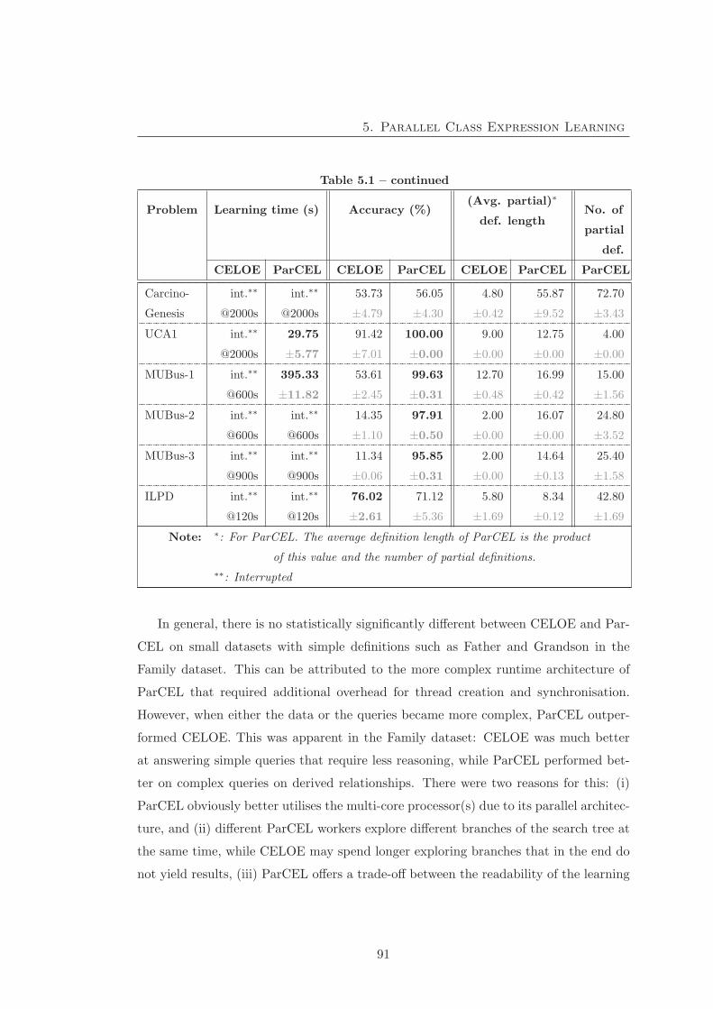
5. Parallel Class Expression Learning
Table 5.1 – continued
Problem Learning time (s) Accuracy (%)(Avg. partial)∗
def. lengthNo. of
partial
def.
CELOE ParCEL CELOE ParCEL CELOE ParCEL ParCEL
Carcino-
Genesis
int.∗∗
@2000s
int.∗∗
@2000s
53.73
±4.79
56.05
±4.30
4.80
±0.42
55.87
±9.52
72.70
±3.43
UCA1 int.∗∗
@2000s
29.75
±5.77
91.42
±7.01
100.00
±0.00
9.00
±0.00
12.75
±0.00
4.00
±0.00
MUBus-1 int.∗∗
@600s
395.33
±11.82
53.61
±2.45
99.63
±0.31
12.70
±0.48
16.99
±0.42
15.00
±1.56
MUBus-2 int.∗∗
@600s
int.∗∗
@600s
14.35
±1.10
97.91
±0.50
2.00
±0.00
16.07
±0.00
24.80
±3.52
MUBus-3 int.∗∗
@900s
int.∗∗
@900s
11.34
±0.06
95.85
±0.31
2.00
±0.00
14.64
±0.13
25.40
±1.58
ILPD int.∗∗
@120s
int.∗∗
@120s
76.02
±2.61
71.12
±5.36
5.80
±1.69
8.34
±0.12
42.80
±1.69
Note: ∗: For ParCEL. The average definition length of ParCEL is the product
of this value and the number of partial definitions.
∗∗: Interrupted
In general, there is no statistically significantly different between CELOE and Par-
CEL on small datasets with simple definitions such as Father and Grandson in the
Family dataset. This can be attributed to the more complex runtime architecture of
ParCEL that required additional overhead for thread creation and synchronisation.
However, when either the data or the queries became more complex, ParCEL outper-
formed CELOE. This was apparent in the Family dataset: CELOE was much better
at answering simple queries that require less reasoning, while ParCEL performed bet-
ter on complex queries on derived relationships. There were two reasons for this: (i)
ParCEL obviously better utilises the multi-core processor(s) due to its parallel architec-
ture, and (ii) different ParCEL workers explore different branches of the search tree at
the same time, while CELOE may spend longer exploring branches that in the end do
not yield results, (iii) ParCEL offers a trade-off between the readability of the learning
91

5. Parallel Class Expression Learning
result and the accuracy and learning time using the combination of specialisation and
generalisation.
Amongst the datasets, the UCA1 dataset (see Section 3.3.3) was chosen to inves-
tigate the capability of the evaluation algorithms in learning long definitions. This is
a noiseless dataset with expected definition length from 30 to more than 50 axioms.
For this dataset, ParCEL outperformed CELOE on both learning time and accuracy.
Although the length of the definition produced by ParCEL was longer than CELOE,
it was readable and described the scenario accurately (positive examples’ definition).
For example, the learnt definition produced by ParCEL for the normal showering was
the disjunction of the following partial definitions:
1. activityHasDuration SOME (hasDurationValue >= 4.5 AND
hasDurationValue <= 15.5)
2. activityHasDuration SOME (hasDurationValue >= 15.5 AND
hasDurationValue <= 19.5) AND activityHasStarttime SOME Spring
3. activityHasDuration SOME (hasDurationValue >= 15.5 AND <= 19.5) AND
activityHasStarttime SOME Summer
4. activityHasStarttime SOME Autumn AND activityHasDuration SOME
(hasDurationValue >= 4.5 AND hasDurationValue <= 19.5)
while CELOE can only generate a definition with length 9 as follows:
activityHasDuration SOME (hasDurationValue >= 4.5 AND
hasDurationValue <= 19.5)
which does not describe the scenario accurately.
One of the most difficult learning problems in the experiment was the CarcinoGen-
esis dataset. Learning results for this dataset reported in [45, 142] shown that CELOE
gave the best accuracy in comparison with other learners with a certain learning con-
figuration. In the experiment, neither CELOE nor ParCEL could find an accurate
definition on the training dataset before they ran out of memory. CELOE ran out of
memory in around 2,100 seconds and ParCEL was be able to run for approximately
92

5. Parallel Class Expression Learning
15,800 seconds with the same JVM heap size. The predictive accuracy of CELOE and
ParCEL on this dataset with 2000s timeout were 54.62% ± 2.71% for CELOE and
55.60% ± 9.52% respectively. The difference between these results was not statistically
significant. The accuracies in Table 5.1 were obtained at 2,000 seconds when CELOE
was approaching the out of memory exception. Although ParCEL was be able to run for
more than 15,800 seconds, we only let it run the same amount of time as CELOE. Our
experiments demonstrated that the accuracy did not improve significantly for longer
runs. Note that this result was generated by the default learning configuration and it
might be different for the refined learning configuration. For example, the predictive
accuracy can be improved by allowing a level of noise in the training dataset. How-
ever, default learning configurations were used for all algorithms and datasets in the
experiments for fair comparisons.
Another noisy dataset is ILPD. For this dataset, CELOE has better predictive accu-
racy than ParCEL. However, this is an unbalanced dataset with the number of positive
examples being more than two times bigger than the number of negative examples:
323 positive examples and 155 negative examples. Therefore, there may be an inflated
performance estimate for CELOE, which favours short definitions. The balanced accu-
racy is reported to work better in this case [87, 121, 134] to avoid inflated performance
estimation. The balanced predictive accuracy is defined as follows:
Definition 5.6 (Balanced accuracy). Given a learning problem LP = 〈K, (E+,E−)〉,C is an expression, then:
balanced accuracy(C, LP) =1
2× (completeness(C,LP ) + correctness(C,LP ))
=1
2×
( |cover(K, C,E+)||E+| +
|E− \ cover(K, C,E−)||E−|
)�
Using the above calculation, the balanced predictive accuracy of CELOE was 64.62%
± 4.83 and that of ParCEL was 70.94 ± 10.87. With this result, CELOE is not statis-
tically significantly more accurate than ParCEL on this dataset.
MUBus-1, MUBus-2 and MUBus-3 are also unbalanced datasets. However, the
number of negative examples is larger than the number of positive examples in these
93

5. Parallel Class Expression Learning
Table 5.2: Balanced accuracy of CELOE and ParCEL on unbalanced datasets (means ±standard deviations of 10 folds). Bold and highlighted values are statistically significantlybetter than the unformatted values in the statistical significance test at 95% confidence.
Dataset CELOE ParCEL
MUBus-1 71.12 ± 0.65 99.68 ±0.60
MUBus-2 52.09 ± 0.06 91.86 ±3.02
MUBus-3 52.18 ± 0.33 73.07 ±1.91
ILDP 64.62 ± 4.83 70.94 ± 10.87
datasets. The balanced predictive accuracy of ParCEL and CELOE on these datasets
were also computed to get a fairer comparison. Originally, predictive accuracy of Par-
CEL on these datasets were much higher than CELOE, e.g. 99.63% ± 0.31% in com-
parison with 53.61% ± 2.45% on MUBus-1 dataset, or 95.85% ± 0.31% in comparison
with 11.34% ± 0.60% on MUBus-3. Using the calculation in Definition 5.6, the bal-
anced accuracies of ParCEL and CELOE on these datasets are given in Table 5.2.
The balanced predictive accuracy of ParCEL on these datasets was still statistically
significantly higher than that of CELOE.
The t-test was used to check the statistical significance of the difference between
learning times of the two algorithms. There were 12 datasets where both the algo-
rithms finished (i.e. without timeout). In those 12 datasets, the t-test rejects the null
hypothesis of 9 of them at the 99% confidence level and one of them at 95% confidence
level. ParCEL had small learning time in all these 9 datasets. Three datasets where
the learning times of CELOE and ParCEL were not statistically significantly different
are Poker-Straight, Father and Grandson, which are the simple datasets with short
definition lengths.
The t-test was also used to check the statistical significant difference of the predictive
accuracy in the experimental results. CELOE and ParCEL achieved 100% predictive
accuracy on 5 datasets. Therefore, they were not tested. In the remaining 11 datasets,
CELOE was statistically significantly more accurate than ParCEL in 1 dataset, ILPD,
and ParCEL was statistically significantly more accurate than CELOE in 5 datasets.
However, CELOE was not statistically significantly more accurate than ParCEL on
94
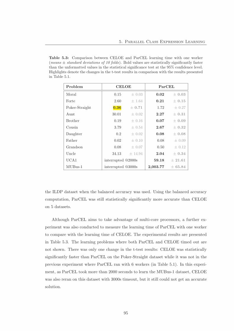
5. Parallel Class Expression Learning
Table 5.3: Comparison between CELOE and ParCEL learning time with one worker(means ± standard deviations of 10 folds). Bold values are statistically significantly fasterthan the unformatted values in the statistical significance test at the 95% confidence level.Highlights denote the changes in the t-test results in comparison with the results presentedin Table 5.1.
Problem CELOE ParCEL
Moral 0.15 ± 0.03 0.02 ± 0.03
Forte 2.60 ± 1.64 0.21 ± 0.15
Poker-Straight 0.36 ± 0.71 1.72 ± 0.27
Aunt 30.01 ± 0.02 2.27 ± 0.31
Brother 0.19 ± 0.16 0.07 ± 0.09
Cousin 3.79 ± 0.54 2.67 ± 0.32
Daughter 0.2 ± 0.02 0.08 ± 0.08
Father 0.02 ± 0.10 0.08 ± 0.09
Grandson 0.08 ± 0.07 0.50 ± 0.12
Uncle 34.13 ± 14.94 2.04 ± 0.34
UCA1 interrupted @2000s 59.18 ± 21.61
MUBus-1 interrupted @3000s 2,003.77 ± 65.84
the ILDP dataset when the balanced accuracy was used. Using the balanced accuracy
computation, ParCEL was still statistically significantly more accurate than CELOE
on 5 datasets.
Although ParCEL aims to take advantage of multi-core processors, a further ex-
periment was also conducted to measure the learning time of ParCEL with one worker
to compare with the learning time of CELOE. The experimental results are presented
in Table 5.3. The learning problems where both ParCEL and CELOE timed out are
not shown. There was only one change in the t-test results: CELOE was statistically
significantly faster than ParCEL on the Poker-Straight dataset while it was not in the
previous experiment where ParCEL ran with 6 workers (in Table 5.1). In this experi-
ment, as ParCEL took more than 2000 seconds to learn the MUBus-1 dataset, CELOE
was also reran on this dataset with 3000s timeout, but it still could not get an accurate
solution.
95
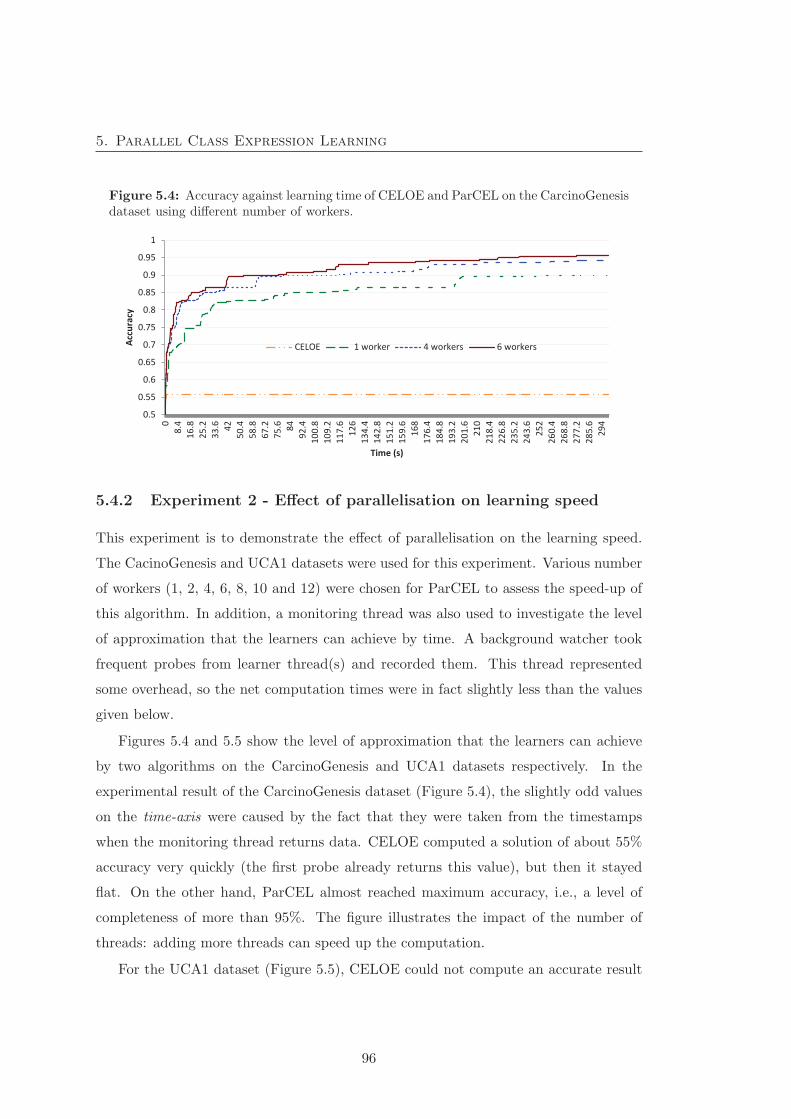
5. Parallel Class Expression Learning
Figure 5.4: Accuracy against learning time of CELOE and ParCEL on the CarcinoGenesisdataset using different number of workers.
0.5
0.55
0.6
0.65
0.7
0.75
0.8
0.85
0.9
0.95
1
08.
416
.825
.233
.6 4250
.458
.867
.275
.6 8492
.410
0.8
109.
211
7.6
126
134.
414
2.8
151.
215
9.6
168
176.
418
4.8
193.
220
1.6
210
218.
422
6.8
235.
224
3.6
252
260.
426
8.8
277.
228
5.6
294
Accu
racy
Time (s)
CELOE 1 worker 4 workers 6 workers
5.4.2 Experiment 2 - Effect of parallelisation on learning speed
This experiment is to demonstrate the effect of parallelisation on the learning speed.
The CacinoGenesis and UCA1 datasets were used for this experiment. Various number
of workers (1, 2, 4, 6, 8, 10 and 12) were chosen for ParCEL to assess the speed-up of
this algorithm. In addition, a monitoring thread was also used to investigate the level
of approximation that the learners can achieve by time. A background watcher took
frequent probes from learner thread(s) and recorded them. This thread represented
some overhead, so the net computation times were in fact slightly less than the values
given below.
Figures 5.4 and 5.5 show the level of approximation that the learners can achieve
by two algorithms on the CarcinoGenesis and UCA1 datasets respectively. In the
experimental result of the CarcinoGenesis dataset (Figure 5.4), the slightly odd values
on the time-axis were caused by the fact that they were taken from the timestamps
when the monitoring thread returns data. CELOE computed a solution of about 55%
accuracy very quickly (the first probe already returns this value), but then it stayed
flat. On the other hand, ParCEL almost reached maximum accuracy, i.e., a level of
completeness of more than 95%. The figure illustrates the impact of the number of
threads: adding more threads can speed up the computation.
For the UCA1 dataset (Figure 5.5), CELOE could not compute an accurate result
96
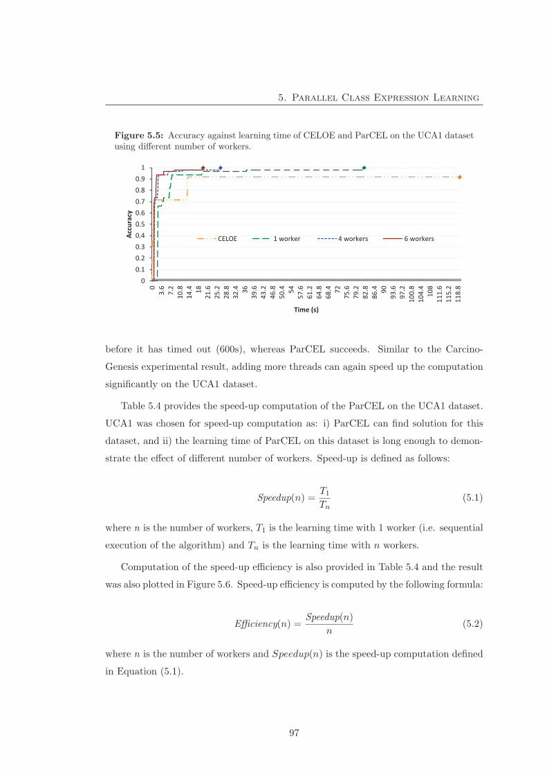
5. Parallel Class Expression Learning
Figure 5.5: Accuracy against learning time of CELOE and ParCEL on the UCA1 datasetusing different number of workers.
00.10.20.30.40.50.60.70.80.9
1
03.
67.
210
.814
.4 1821
.625
.228
.832
.4 3639
.643
.246
.850
.4 5457
.661
.264
.868
.4 7275
.679
.282
.886
.4 9093
.697
.210
0.8
104.
410
811
1.6
115.
211
8.8
Accu
racy
Time (s)
CELOE 1 worker 4 workers 6 workers
before it has timed out (600s), whereas ParCEL succeeds. Similar to the Carcino-
Genesis experimental result, adding more threads can again speed up the computation
significantly on the UCA1 dataset.
Table 5.4 provides the speed-up computation of the ParCEL on the UCA1 dataset.
UCA1 was chosen for speed-up computation as: i) ParCEL can find solution for this
dataset, and ii) the learning time of ParCEL on this dataset is long enough to demon-
strate the effect of different number of workers. Speed-up is defined as follows:
Speedup(n) =T1
Tn(5.1)
where n is the number of workers, T1 is the learning time with 1 worker (i.e. sequential
execution of the algorithm) and Tn is the learning time with n workers.
Computation of the speed-up efficiency is also provided in Table 5.4 and the result
was also plotted in Figure 5.6. Speed-up efficiency is computed by the following formula:
Efficiency(n) =Speedup(n)
n(5.2)
where n is the number of workers and Speedup(n) is the speed-up computation defined
in Equation (5.1).
97

5. Parallel Class Expression Learning
Table 5.4: Speed-up of ParCEL on the UCA1 dataset. The learning time of CELOE isincluded for comparison. CELOE was timeout after 600 seconds.
Workers CELOE 1 2 4 6 8 10 12
Learning time (s) 600.00 86.48 46.23 27.00 20.11 16.52 19.40 19.15
Speedup 1.00 1.00 1.87 3.20 4.30 5.24 4.46 4.62
Efficiency 1.00 1.00 0.94 0.80 0.72 0.65 0.45 0.38
Figure 5.6: Speed-up efficiency of ParCEL on the UCA1 dataset.
1 0.94
0.80 0.72
0.65
0.45 0.38
0
0.2
0.4
0.6
0.8
1
1.2
1 2 4 6 8 10 12
Effic
icen
cy
Number of workers
5.4.3 Experiment 3 - Definition reduction strategy
This experiment is to compare the three reduction algorithms discussed earlier. Here,
the length of descriptions was measured and the number of descriptions produced was
counted. To compare the description length, the method defined above was used, i.e.,
the lengths of the virtual disjunction we could create from the set of partial definitions
were measured. To keep the result concise, we used only some of datasets in this
experiment that cover sufficient space of cases, i.e. simple to complex, short to long
definition. A comparison between reduction strategies is given in Table 5.5.
The results shows that GMPC gave the shortest definition in most of the experi-
ments and thus the definitions are more readable, while GORL produced the longest
definitions in all the experiments. However, GMPC requires all partial definitions to be
kept until the learning finishes, while GORL can perform the reduction on-the-fly while
the learning algorithm is running. This may offer a trade-off between the readability of
the learnt definition and the memory used by the learner as well as the learning time.
98
5. Parallel Class Expression Learning
In all experiments, GMPC was used as the default reduction strategy as it produced
shorter definitions than the other strategies. The GORL strategy is similar to the
generalisation process in DL-FOIL.
Table 5.5: Definition length comparison between three reduction strategies (means ±standard deviations of 10 folds). The bold values are statistically significantly better thanthe other values; the unformatted values are statistically significantly worse than the othervalues; the bold and italic values are statistically significantly better than the unformattedvalues and statistically significantly worse than the bold values in the statistical significancetest at 95% confidence.
DatasetGMPC GOLR GMPL
avg.
partial
def.
length
no. of
partial
def.
avg.
partial
def.
length
no. of
partial
def.
avg.
partial
def.
length
no. of
partial
def.
Moral 1.52
±0.05
2.10
±0.32
2.15
±1.26
3.40
±0.97
1.67
±0.00
3.00
±0.00
Forte 7.75
±0.50
2.00
±0.00
7.71
±0.43
2.30
±0.68
7.62
±0.21
2.30
±0.68
Poker-straight 10.90
±1.31
1.70
±0.68
9.88
±1.46
2.70
±0.48
9.48
±0.98
2.70
±0.48
Aunt 8.80
±0.48
2.00
±0.00
7.75
±0.29
8.90
±2.08
7.48
±0.31
8.30
±1.42
Brother 6.00
±1.83
1.00
±0.00
5.60
±0.52
1.00
±0.00
5.10
±0.32
1.00
±0.00
Cousin 8.50
±0.00
2.00
±0.00
8.50
±0.58
8.20
±4.16
8.10
±0.21
5.70
±1.25
Daughter 5.25
±1.09
1.10
±0.32
7.55
±2.41
1.50
±0.53
5.33
±0.47
1.40
±0.84
Father 5.50
±0.53
1.00
±0.00
5.20
±0.42
1.00
±0.00
5.30
±0.48
1.00
±0.00
Grandson 7.25
±0.50
1.00
±0.00
7.53
±0.55
2.90
±0.57
7.20
±0.50
2.5
±0.71
Uncle 8.40
±0.38
3.00
±0.00
7.92
±0.16
7.10
±1.29
7.75
±0.48
6.80
±1.14
Continued on next page
99
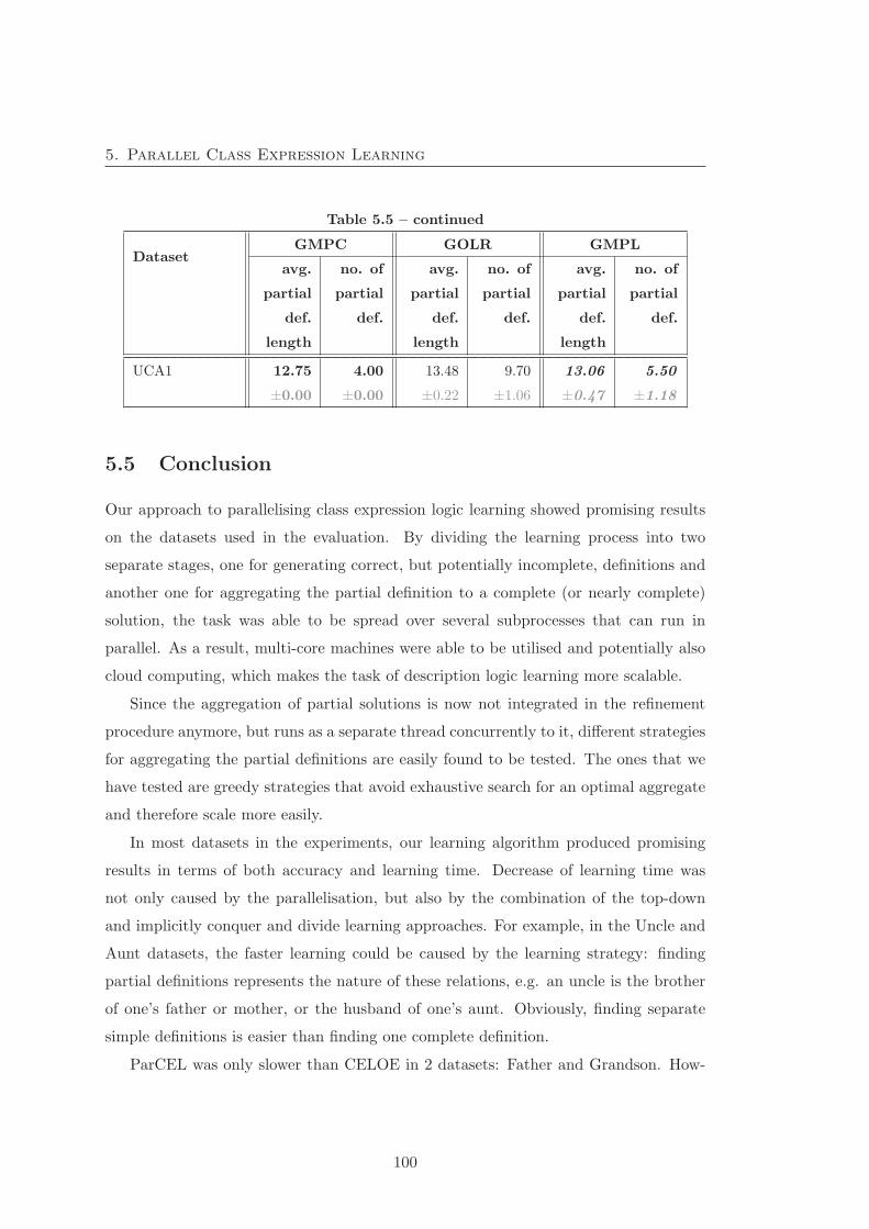
5. Parallel Class Expression Learning
Table 5.5 – continued
DatasetGMPC GOLR GMPL
avg.
partial
def.
length
no. of
partial
def.
avg.
partial
def.
length
no. of
partial
def.
avg.
partial
def.
length
no. of
partial
def.
UCA1 12.75
±0.00
4.00
±0.00
13.48
±0.22
9.70
±1.06
13.06
±0.47
5.50
±1.18
5.5 Conclusion
Our approach to parallelising class expression logic learning showed promising results
on the datasets used in the evaluation. By dividing the learning process into two
separate stages, one for generating correct, but potentially incomplete, definitions and
another one for aggregating the partial definition to a complete (or nearly complete)
solution, the task was able to be spread over several subprocesses that can run in
parallel. As a result, multi-core machines were able to be utilised and potentially also
cloud computing, which makes the task of description logic learning more scalable.
Since the aggregation of partial solutions is now not integrated in the refinement
procedure anymore, but runs as a separate thread concurrently to it, different strategies
for aggregating the partial definitions are easily found to be tested. The ones that we
have tested are greedy strategies that avoid exhaustive search for an optimal aggregate
and therefore scale more easily.
In most datasets in the experiments, our learning algorithm produced promising
results in terms of both accuracy and learning time. Decrease of learning time was
not only caused by the parallelisation, but also by the combination of the top-down
and implicitly conquer and divide learning approaches. For example, in the Uncle and
Aunt datasets, the faster learning could be caused by the learning strategy: finding
partial definitions represents the nature of these relations, e.g. an uncle is the brother
of one’s father or mother, or the husband of one’s aunt. Obviously, finding separate
simple definitions is easier than finding one complete definition.
ParCEL was only slower than CELOE in 2 datasets: Father and Grandson. How-
100
5. Parallel Class Expression Learning
ever, these are very small datasets with short definitions: from 5 to 7 axioms, and the
differences between learning times were not statistically significant. In addition, this is
not our objective as the algorithm is expected to deal with complex learning problems.
For the noisy dataset CarcinoGenesis, ParCEL could not give a better result than
CELOE, which shows that our learning currently might not deal well with noisy data
and this is a future development so that the algorithm can deal with various learning
problems. For another noisy dataset ILPD, ParCEL predictive accuracy was lower than
CELOE. However, it was caused by the imbalance between positive and negative ex-
amples. A further investigation showed that our learning algorithm was more accurate
if the balanced predictive accuracy was used.
A disadvantage of our learning approach is that it produced longer definitions than
CELOE. In some circumstances, long definitions were needed to describe accurately the
learning problems. However, there were also unnecessarily long definitions caused by
overlap between partial definitions. Using normalisation and simplification can reduce
the definition length [3, 51, 65, 86]. This has not been implemented yet and is left for
future work.
101

5. Parallel Class Expression Learning
102
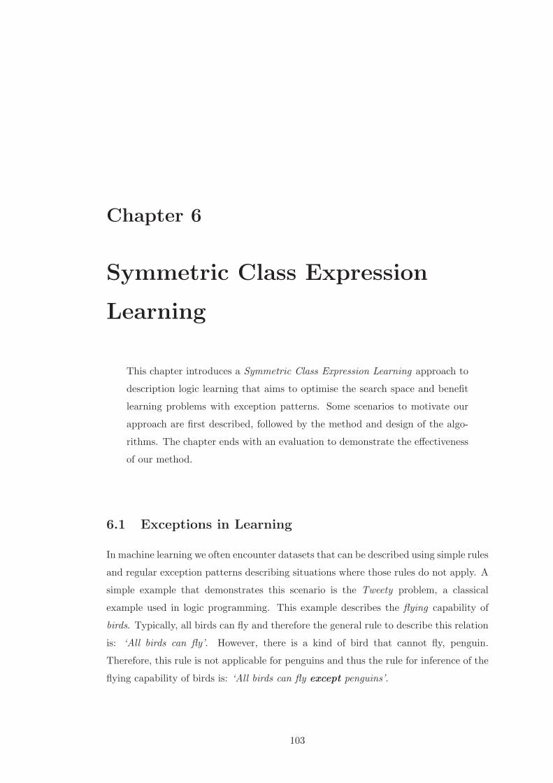
Chapter 6
Symmetric Class Expression
Learning
This chapter introduces a Symmetric Class Expression Learning approach to
description logic learning that aims to optimise the search space and benefit
learning problems with exception patterns. Some scenarios to motivate our
approach are first described, followed by the method and design of the algo-
rithms. The chapter ends with an evaluation to demonstrate the effectiveness
of our method.
6.1 Exceptions in Learning
In machine learning we often encounter datasets that can be described using simple rules
and regular exception patterns describing situations where those rules do not apply. A
simple example that demonstrates this scenario is the Tweety problem, a classical
example used in logic programming. This example describes the flying capability of
birds. Typically, all birds can fly and therefore the general rule to describe this relation
is: ‘All birds can fly’. However, there is a kind of bird that cannot fly, penguin.
Therefore, this rule is not applicable for penguins and thus the rule for inference of the
flying capability of birds is: ‘All birds can fly except penguins’.
103
6. Symmetric Class Expression Learning
Another scenario is the problem of learning inhabitant’s normal behaviours in houses
such as in the UCA1 dataset (see Chapter 3). In this scenario, it is often the case that
a normal behaviour can consist of a general rule and then a set of exceptions. For
example, a person may usually go to the library at 9AM on Mondays. However, this
pattern might be broken by particular circumstances such as rain, or public holidays.
Therefore, rather than ‘The person goes to the library on Mondays at 9AM’, the rule
becomes ‘The person goes to the library on Mondays at 9AM as long as it is not
raining and it is not a public holiday’.
The term exception is used in this sense: a small set of examples that are incorrectly
covered by simple concepts that describe the vast majority of examples correctly. In
the above examples, ‘All bird can fly’ and ‘The person goes to the library on Monday
at 9AM’ are the general rules that describe the normal flying ability and going to
library activity pattern of most of birds and going to library activities respectively.
Penguins, rain and public holidays are the exceptions in these scenarios that require
further constraints (rules) to make the general rules correct.
Most existing DL learning algorithms, e.g. AL−QuIn [85], DL-FOIL [45], CELOE
[82] and ParCEL (Chapter 5), focus only on the definitions of positive examples. Learn-
ing starts from a very general concept, usually the TOP concept in DL. Then, subclasses
and sub-properties (specialisation), conjunction (intersection) and the combination of
conjunction and negation (subtraction) are used to remove the negative examples from
the potential concepts.
This approach suits many learning problems and has been used successfully in
[57, 82] and the experiments in Chapter 5. However, this strategy does not deal very
well with learning problems that have exceptions to the normal patterns. It also does
not use the descriptions in the search space effectively. Here CELOE and ParCEL are
used as representative algorithms for two different approaches, the top-down and the
combination of top-down and bottom-up approaches, to demonstrate the weakness of
these approaches in dealing with exceptions in learning. Given a learning problem with
a set of positive (+) and negative (–) examples, the concepts D1, D2, N1, N2 and their
coverage (Figure 6.1(a)), top-down learning algorithms such as CELOE [82] find the
single concept C = (D1 � ¬N1) � (D2 � ¬N2), algorithms that combine both top-down
104
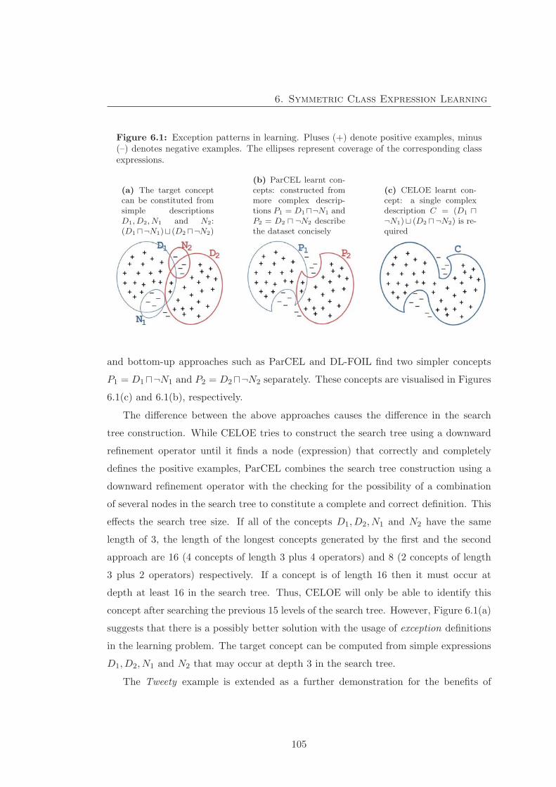
6. Symmetric Class Expression Learning
Figure 6.1: Exception patterns in learning. Pluses (+) denote positive examples, minus(–) denotes negative examples. The ellipses represent coverage of the corresponding classexpressions.
(a) The target conceptcan be constituted fromsimple descriptionsD1, D2, N1 and N2:(D1�¬N1)� (D2�¬N2)
(b) ParCEL learnt con-cepts: constructed frommore complex descrip-tions P1 = D1�¬N1 andP2 = D2 � ¬N2 describethe dataset concisely
(c) CELOE learnt con-cept: a single complexdescription C = (D1 �¬N1)� (D2 �¬N2) is re-quired
and bottom-up approaches such as ParCEL and DL-FOIL find two simpler concepts
P1 = D1�¬N1 and P2 = D2�¬N2 separately. These concepts are visualised in Figures
6.1(c) and 6.1(b), respectively.
The difference between the above approaches causes the difference in the search
tree construction. While CELOE tries to construct the search tree using a downward
refinement operator until it finds a node (expression) that correctly and completely
defines the positive examples, ParCEL combines the search tree construction using a
downward refinement operator with the checking for the possibility of a combination
of several nodes in the search tree to constitute a complete and correct definition. This
effects the search tree size. If all of the concepts D1, D2, N1 and N2 have the same
length of 3, the length of the longest concepts generated by the first and the second
approach are 16 (4 concepts of length 3 plus 4 operators) and 8 (2 concepts of length
3 plus 2 operators) respectively. If a concept is of length 16 then it must occur at
depth at least 16 in the search tree. Thus, CELOE will only be able to identify this
concept after searching the previous 15 levels of the search tree. However, Figure 6.1(a)
suggests that there is a possibly better solution with the usage of exception definitions
in the learning problem. The target concept can be computed from simple expressions
D1, D2, N1 and N2 that may occur at depth 3 in the search tree.
The Tweety example is extended as a further demonstration for the benefits of
105

6. Symmetric Class Expression Learning
using the definitions of exceptions in learning as shown in Figure 6.2. This figure
represents a search tree for the three learning strategies described above. As was
discussed above, finding a complete definition (triple-line node, e.g. CELOE) requires
a deeper search tree than finding several partial definitions (double-line nodes, e.g.
ParCEL, DL-FOIL). Moreover, using definition of exceptions (dotted-line nodes) can
produce shallower search trees.
6.2 Symmetric Class Expression Learning
6.2.1 Overview of our method
To address the problem described in Section 6.1, a Symmetric Class Expression Learn-
ing (SPaCEL) learning approach is proposed that processes the positive and negative
examples symmetrically and simultaneously. Definitions of both positive and negative
examples are sought separately and then they are combined to construct a complete
definition. The negative example definitions are used to remove the negative examples
from the concepts in the search tree to create definitions for positive examples. This
learning approach can combine (potentially very short) concepts and so define relatively
complex concepts based on much smaller depth traversals. This is particularly useful
where removing negative examples leads to shorter definitions of positive examples.
Consequently, concepts in the search tree are used more effectively. It helps to
reduce the search space of the learning problem and thus the learning time can be re-
duced. This approach is best suited to learning problems with exceptions as described
in Section 6.1, especially when the exceptions follow a few relatively simple patterns. A
simple pattern corresponds to a short, and therefore easily comprehensible, definition.
Here, the pattern is used analogously to the definition in the context of description
logics, i.e. a description that describes the characteristics of a set of examples. These
benefits can help the learning approach to be more scalable with respect to the com-
plexity of the learnt concept (definition length). Table 6.1 summarises the usage of
positive and negative examples in learning of basic description logic learning.
106
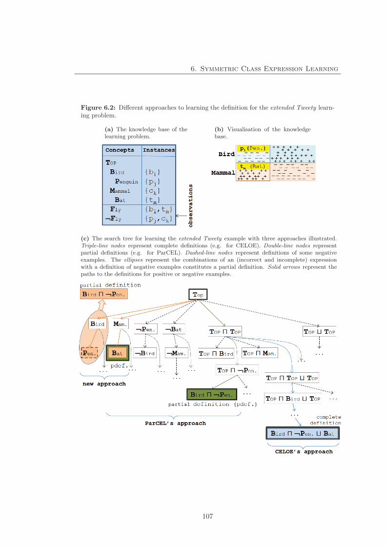
6. Symmetric Class Expression Learning
Figure 6.2: Different approaches to learning the definition for the extended Tweety learn-ing problem.
(a) The knowledge base of thelearning problem.
(b) Visualisation of the knowledgebase.
(c) The search tree for learning the extended Tweety example with three approaches illustrated.Triple-line nodes represent complete definitions (e.g. for CELOE). Double-line nodes representpartial definitions (e.g. for ParCEL). Dashed-line nodes represent definitions of some negativeexamples. The ellipses represent the combinations of an (incorrect and incomplete) expressionwith a definition of negative examples constitutes a partial definition. Solid arrows represent thepaths to the definitions for positive or negative examples.
107

6. Symmetric Class Expression Learning
Table 6.1: Basic description learning algorithms and their usage of examples.
Type of pattern Our approach(SPaCEL)
YinYang Others, e.g. CELOE,ParCEL, DL-FOIL
positive patterns top-down top-down top-down
negative patterns top-down bottom-up –
6.2.2 Description of our method
In this learning approach, the positive and negative examples are used symmetrically.
Definitions of both positive and negative examples are employed to learn the final
definition. Basically, our learning approach consists of three main steps:
1. Find the definitions for positive and negative examples such that all the defini-
tions, together, cover all positive or negative examples.
2. Reduce the partial definitions to remove the redundancies and select the best
candidates for constructing a complete definition.
3. Aggregate the best candidates to form the complete definition using disjunction.
In the first step, partial definitions can be produced directly by specialisation using
a downward refinement operator as in some other algorithms such as DL-FOIL and
ParCEL. In this approach, as was described in Section 6.1, beside the partial definitions,
the definitions of negative examples are also computed and used in combination with
existing expressions in the search tree to create partial definitions.
Definitions of negative examples are called counter-partial definitions. They are
formally defined as follows:
Definition 6.1 (Counter-partial definition). Given a learning problem LP = 〈K,
(E+,E−)〉 as defined in Definition 2.16, a class expression C is called a counter-partial
definition if cover(K, C,E−) = ∅ and cover(K, C,E−) �= ∅. �
The top-down step consists of the usage of a refinement operator to find the partial
definitions and counter-partial definitions, and a combination operator to compute more
partial definitions from the counter-partial definitions and existing expressions in the
108
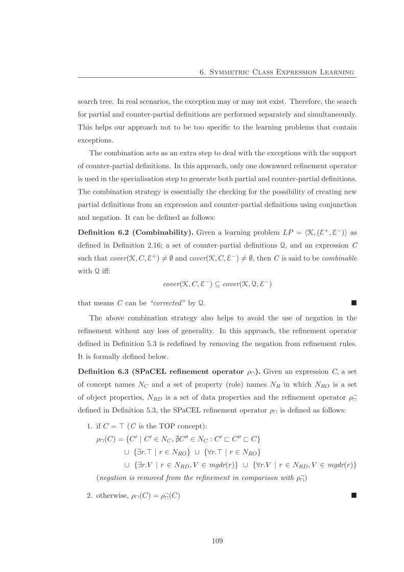
6. Symmetric Class Expression Learning
search tree. In real scenarios, the exception may or may not exist. Therefore, the search
for partial and counter-partial definitions are performed separately and simultaneously.
This helps our approach not to be too specific to the learning problems that contain
exceptions.
The combination acts as an extra step to deal with the exceptions with the support
of counter-partial definitions. In this approach, only one downward refinement operator
is used in the specialisation step to generate both partial and counter-partial definitions.
The combination strategy is essentially the checking for the possibility of creating new
partial definitions from an expression and counter-partial definitions using conjunction
and negation. It can be defined as follows:
Definition 6.2 (Combinability). Given a learning problem LP = 〈K, (E+,E−)〉 as
defined in Definition 2.16; a set of counter-partial definitions Q, and an expression C
such that cover(K, C,E+) �= ∅ and cover(K, C,E−) �= ∅, then C is said to be combinable
with Q iff:
cover(K, C,E−) ⊆ cover(K,Q,E−)
that means C can be “corrected” by Q. �
The above combination strategy also helps to avoid the use of negation in the
refinement without any loss of generality. In this approach, the refinement operator
defined in Definition 5.3 is redefined by removing the negation from refinement rules.
It is formally defined below.
Definition 6.3 (SPaCEL refinement operator ρ�). Given an expression C, a set
of concept names NC and a set of property (role) names NR in which NRO is a set
of object properties, NRD is a set of data properties and the refinement operator ρ¬�defined in Definition 5.3, the SPaCEL refinement operator ρ� is defined as follows:
1. if C = (C is the TOP concept):
ρ�(C) = {C ′ | C ′ ∈ NC , �C ′′ ∈ NC : C ′ � C ′′ � C}∪ {∃r. | r ∈ NRO} ∪ {∀r. | r ∈ NRO}∪ {∃r.V | r ∈ NRD, V ∈ mgdr(r)} ∪ {∀r.V | r ∈ NRD, V ∈ mgdr(r)}
(negation is removed from the refinement in comparison with ρ¬�)
2. otherwise, ρ�(C) = ρ¬�(C) �
109
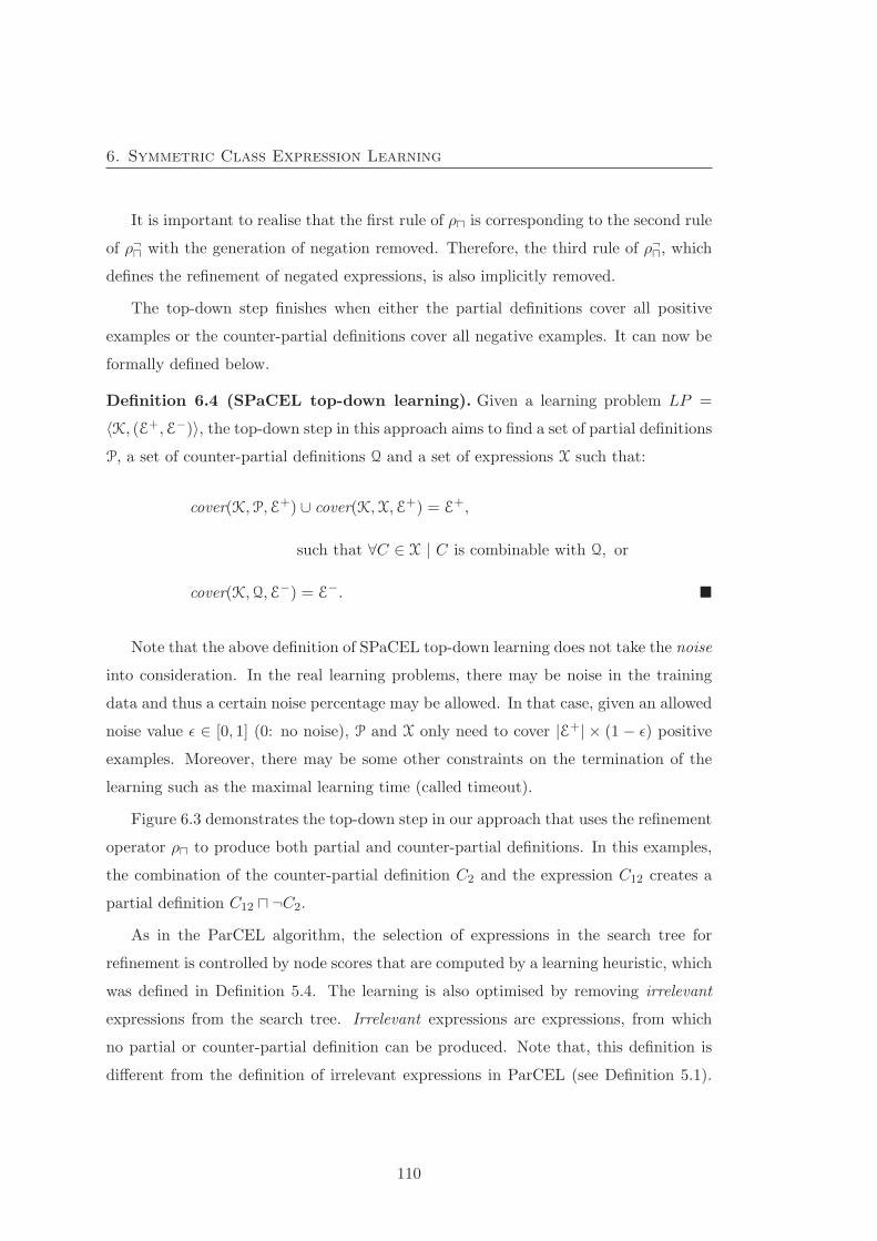
6. Symmetric Class Expression Learning
It is important to realise that the first rule of ρ� is corresponding to the second rule
of ρ¬� with the generation of negation removed. Therefore, the third rule of ρ¬�, which
defines the refinement of negated expressions, is also implicitly removed.
The top-down step finishes when either the partial definitions cover all positive
examples or the counter-partial definitions cover all negative examples. It can now be
formally defined below.
Definition 6.4 (SPaCEL top-down learning). Given a learning problem LP =
〈K, (E+,E−)〉, the top-down step in this approach aims to find a set of partial definitions
P, a set of counter-partial definitions Q and a set of expressions X such that:
cover(K,P,E+) ∪ cover(K,X,E+) = E+,
such that ∀C ∈ X | C is combinable with Q, or
cover(K,Q,E−) = E−. �
Note that the above definition of SPaCEL top-down learning does not take the noise
into consideration. In the real learning problems, there may be noise in the training
data and thus a certain noise percentage may be allowed. In that case, given an allowed
noise value ε ∈ [0, 1] (0: no noise), P and X only need to cover |E+| × (1 − ε) positive
examples. Moreover, there may be some other constraints on the termination of the
learning such as the maximal learning time (called timeout).
Figure 6.3 demonstrates the top-down step in our approach that uses the refinement
operator ρ� to produce both partial and counter-partial definitions. In this examples,
the combination of the counter-partial definition C2 and the expression C12 creates a
partial definition C12 � ¬C2.
As in the ParCEL algorithm, the selection of expressions in the search tree for
refinement is controlled by node scores that are computed by a learning heuristic, which
was defined in Definition 5.4. The learning is also optimised by removing irrelevant
expressions from the search tree. Irrelevant expressions are expressions, from which
no partial or counter-partial definition can be produced. Note that, this definition is
different from the definition of irrelevant expressions in ParCEL (see Definition 5.1).
110
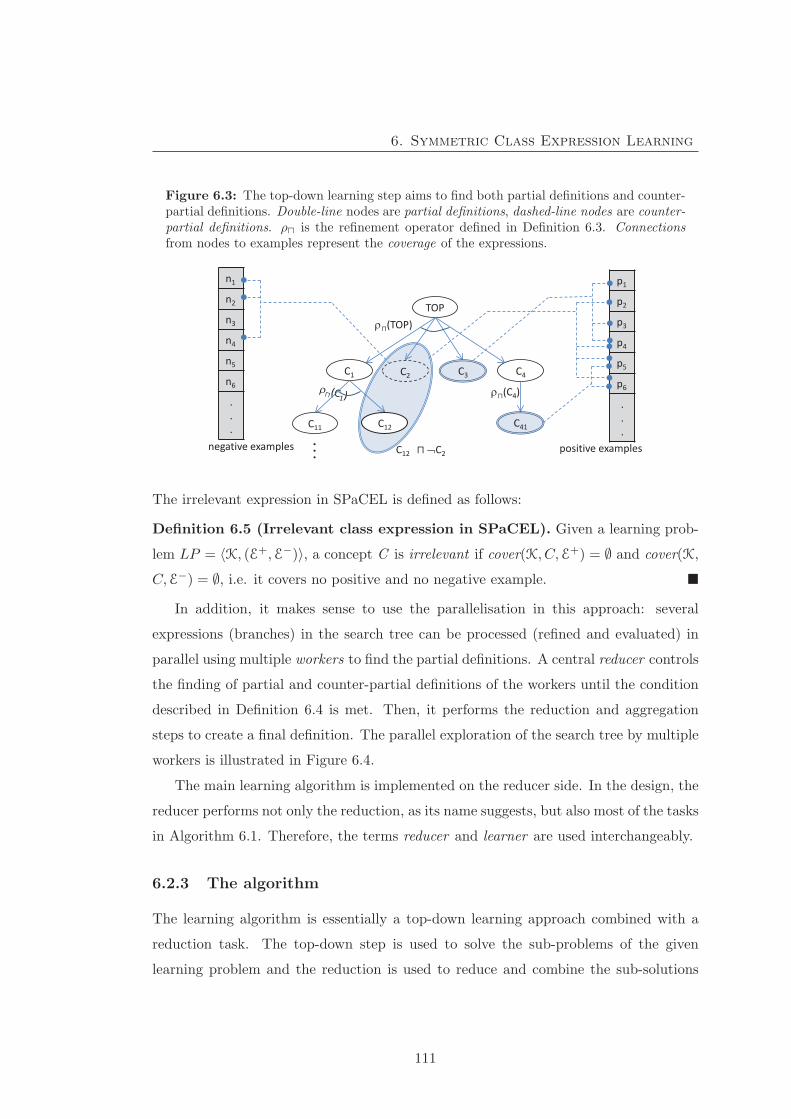
6. Symmetric Class Expression Learning
Figure 6.3: The top-down learning step aims to find both partial definitions and counter-partial definitions. Double-line nodes are partial definitions, dashed-line nodes are counter-partial definitions. ρ� is the refinement operator defined in Definition 6.3. Connectionsfrom nodes to examples represent the coverage of the expressions.
(TOP) TOP
C1 C4
C11 C12
(C4)
p1
p2
p3
p4
p5
p6
.
.
. . . .
C41
C2
positive examples
n1
n2
n3
n4
n5
n6
.
.
. negative examples
C3
C12 C2
The irrelevant expression in SPaCEL is defined as follows:
Definition 6.5 (Irrelevant class expression in SPaCEL). Given a learning prob-
lem LP = 〈K, (E+,E−)〉, a concept C is irrelevant if cover(K, C,E+) = ∅ and cover(K,
C,E−) = ∅, i.e. it covers no positive and no negative example. �
In addition, it makes sense to use the parallelisation in this approach: several
expressions (branches) in the search tree can be processed (refined and evaluated) in
parallel using multiple workers to find the partial definitions. A central reducer controls
the finding of partial and counter-partial definitions of the workers until the condition
described in Definition 6.4 is met. Then, it performs the reduction and aggregation
steps to create a final definition. The parallel exploration of the search tree by multiple
workers is illustrated in Figure 6.4.
The main learning algorithm is implemented on the reducer side. In the design, the
reducer performs not only the reduction, as its name suggests, but also most of the tasks
in Algorithm 6.1. Therefore, the terms reducer and learner are used interchangeably.
6.2.3 The algorithm
The learning algorithm is essentially a top-down learning approach combined with a
reduction task. The top-down step is used to solve the sub-problems of the given
learning problem and the reduction is used to reduce and combine the sub-solutions
111
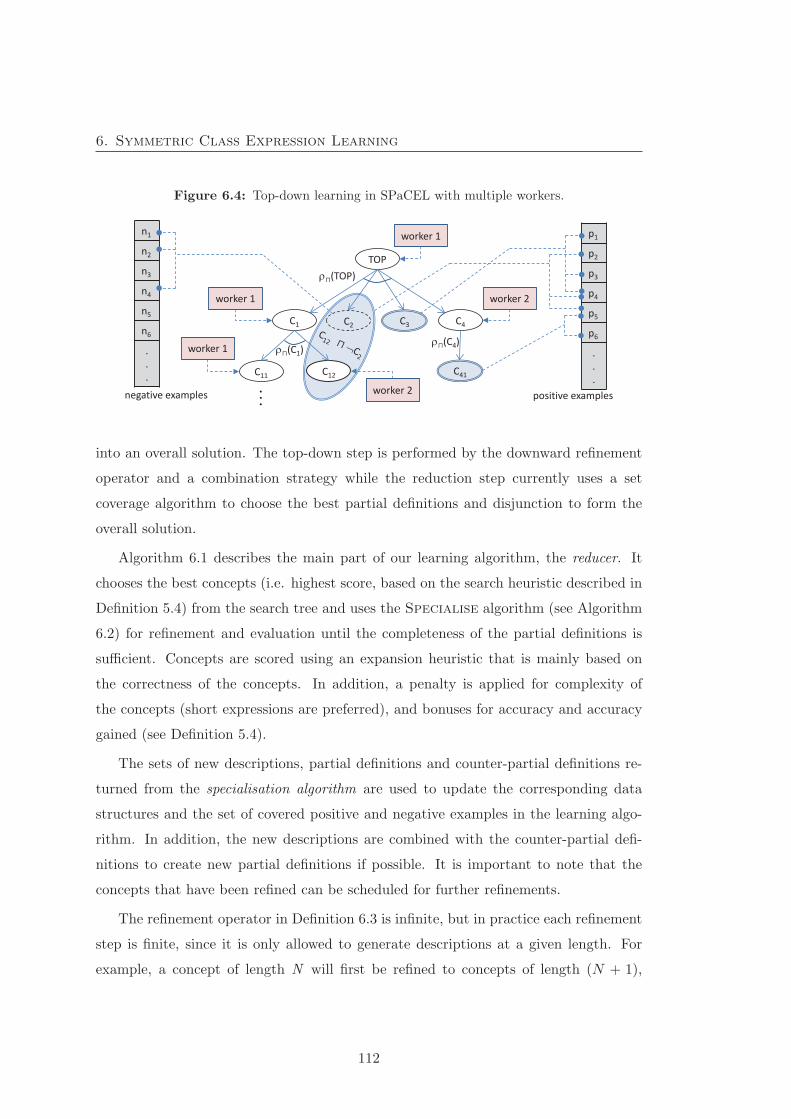
6. Symmetric Class Expression Learning
Figure 6.4: Top-down learning in SPaCEL with multiple workers.
(TOP)
(C1)
TOP
C1 C4
C11 C12
(C4)
worker 1
worker 1
worker 1
worker 2
p1
p2
p3
p4
p5
p6
.
.
.
worker 2
C3
. . .
C41
C2
positive examples
n1
n2
n3
n4
n5
n6
.
.
.
negative examples
into an overall solution. The top-down step is performed by the downward refinement
operator and a combination strategy while the reduction step currently uses a set
coverage algorithm to choose the best partial definitions and disjunction to form the
overall solution.
Algorithm 6.1 describes the main part of our learning algorithm, the reducer. It
chooses the best concepts (i.e. highest score, based on the search heuristic described in
Definition 5.4) from the search tree and uses the Specialise algorithm (see Algorithm
6.2) for refinement and evaluation until the completeness of the partial definitions is
sufficient. Concepts are scored using an expansion heuristic that is mainly based on
the correctness of the concepts. In addition, a penalty is applied for complexity of
the concepts (short expressions are preferred), and bonuses for accuracy and accuracy
gained (see Definition 5.4).
The sets of new descriptions, partial definitions and counter-partial definitions re-
turned from the specialisation algorithm are used to update the corresponding data
structures and the set of covered positive and negative examples in the learning algo-
rithm. In addition, the new descriptions are combined with the counter-partial defi-
nitions to create new partial definitions if possible. It is important to note that the
concepts that have been refined can be scheduled for further refinements.
The refinement operator in Definition 6.3 is infinite, but in practice each refinement
step is finite, since it is only allowed to generate descriptions at a given length. For
example, a concept of length N will first be refined to concepts of length (N + 1),
112
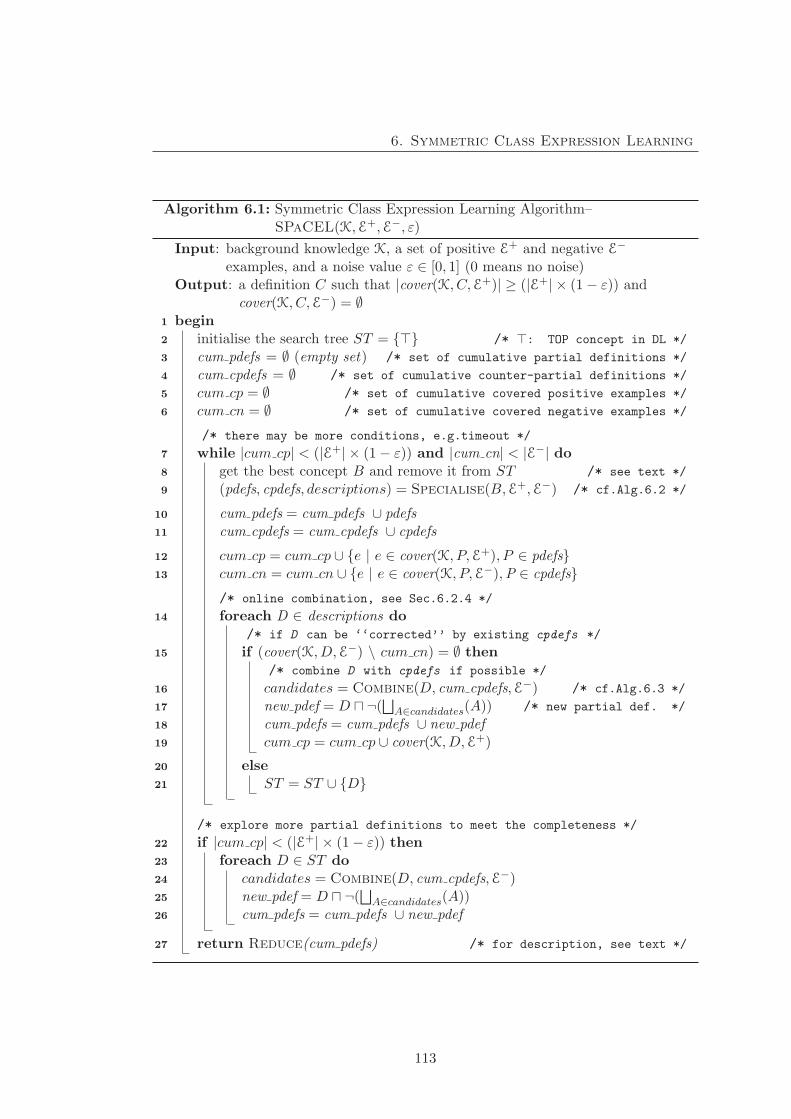
6. Symmetric Class Expression Learning
Algorithm 6.1: Symmetric Class Expression Learning Algorithm–SPaCEL(K,E+,E−, ε)
Input: background knowledge K, a set of positive E+ and negative E−
examples, and a noise value ε ∈ [0, 1] (0 means no noise)Output: a definition C such that |cover(K, C,E+)| ≥ (|E+| × (1− ε)) and
cover(K, C,E−) = ∅1 begin2 initialise the search tree ST = {} /* : TOP concept in DL */
3 cum pdefs = ∅ (empty set) /* set of cumulative partial definitions */
4 cum cpdefs = ∅ /* set of cumulative counter-partial definitions */
5 cum cp = ∅ /* set of cumulative covered positive examples */
6 cum cn = ∅ /* set of cumulative covered negative examples */
/* there may be more conditions, e.g.timeout */
7 while |cum cp| < (|E+| × (1− ε)) and |cum cn| < |E−| do8 get the best concept B and remove it from ST /* see text */
9 (pdefs, cpdefs, descriptions) = Specialise(B,E+,E−) /* cf.Alg.6.2 */
10 cum pdefs = cum pdefs ∪ pdefs11 cum cpdefs = cum cpdefs ∪ cpdefs
12 cum cp = cum cp ∪ {e | e ∈ cover(K, P,E+), P ∈ pdefs}13 cum cn = cum cn ∪ {e | e ∈ cover(K, P,E−),P ∈ cpdefs}
/* online combination, see Sec.6.2.4 */
14 foreach D ∈ descriptions do/* if D can be ‘‘corrected’’ by existing cpdefs */
15 if (cover(K, D,E−) \ cum cn) = ∅ then/* combine D with cpdefs if possible */
16 candidates = Combine(D, cum cpdefs,E−) /* cf.Alg.6.3 */
17 new pdef = D � ¬(⊔A∈candidates(A)) /* new partial def. */
18 cum pdefs = cum pdefs ∪ new pdef19 cum cp = cum cp ∪ cover(K, D,E+)
20 else21 ST = ST ∪ {D}
/* explore more partial definitions to meet the completeness */
22 if |cum cp| < (|E+| × (1− ε)) then23 foreach D ∈ ST do24 candidates = Combine(D, cum cpdefs,E−)25 new pdef = D � ¬(⊔A∈candidates(A))26 cum pdefs = cum pdefs ∪ new pdef
27 return Reduce(cum pdefs) /* for description, see text */
113

6. Symmetric Class Expression Learning
and later, when it is revisited, to concepts of length (N + 2), etc. For the sake of
simplicity, we use ρ� in the algorithms to refer to one refinement step rather than the
entire refinement. This technique is used in DL-Learner and discussed in detail in [82].
When the algorithm reaches a sufficient degree of completeness, it stops and reduces
the partial definitions to remove the redundancies using the Reduce function, which
is essentially a set coverage algorithm: given a set of partial definitions X and a set
of positive examples E+, it finds a subset X′ ⊆ X such that E+ ⊆ ⋃D∈X′(cover(K, D,
E+)). The solution returned by the algorithm is a disjunction of the reduced partial
definitions. However, returning the result as a set of partial definitions instead may be
useful in some contexts, e.g. to make the result more readable. The reduction algo-
rithm may be tailored to meet particular requirements such as the shortest definition
or the least number of partial definitions. Note that the combination of descriptions
and counter-partial definitions in Algorithm 6.1 is one of the combination strategies
implemented in our evaluation. This strategy is called an on-the-fly combination strat-
egy; it gave the best performance in our evaluation (see Section 6.3.1). A discussion of
the combination strategies is given in Section 6.2.4.
The specialisation is described in Algorithm 6.2. The specialisation performs the
refinement and evaluation of the concepts assigned by the learning algorithm. Firstly, it
refines the given concept (ρ�(C)) and evaluates the result (cover(K, C,E+) and cover(K,
C,E−)). Irrelevant concepts are removed from the result as no partial definition or
counter-partial definition can be computed though the irrelevant concept specification.
Then, the specialisation finds new partial definitions, counter-partial definitions and
descriptions from the refinements. Practically, redundancies are often checked before
evaluating descriptions to avoid redundant evaluations and duplicated descriptions in
the search tree as a description can be generated from different branches.
Algorithm 6.3 describes the combination algorithm that is used to combine the
descriptions and counter-partial definitions to construct new partial definitions. This
is basically a set coverage algorithm. A smallest set of counter-partial definitions that
together cover all negative examples covered by the given expression will be returned.
This set of counter-partial definitions is then used to correct the given expression.
114
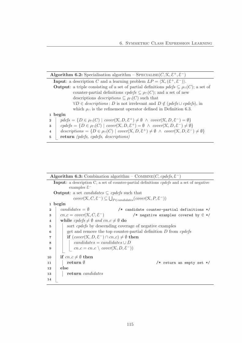
6. Symmetric Class Expression Learning
Algorithm 6.2: Specialisation algorithm – Specialise(C,K,E+,E−)Input: a description C and a learning problem LP = 〈K, (E+,E−)〉.Output: a triple consisting of a set of partial definitions pdefs ⊆ ρ�(C); a set of
counter-partial definitions cpdefs ⊆ ρ�(C); and a set of newdescriptions descriptions ⊆ ρ�(C) such that∀D ∈ descriptions : D is not irrelevant and D /∈ (pdefs ∪ cpdefs), inwhich ρ� is the refinement operator defined in Definition 6.3.
1 begin2 pdefs = {D ∈ ρ�(C) | cover(K, D,E+) �= ∅ ∧ cover(K, D,E−) = ∅}3 cpdefs = {D ∈ ρ�(C) | cover(K, D,E+) = ∅ ∧ cover(K, D,E−) �= ∅}4 descriptions = {D ∈ ρ�(C) | cover(K, D,E+) �= ∅ ∧ cover(K, D,E−) �= ∅}5 return (pdefs, cpdefs, descriptions)
Algorithm 6.3: Combination algorithm – Combine(C, cpdefs,E−)Input: a description C, a set of counter-partial definitions cpdefs and a set of negative
examples E−
Output: a set candidates ⊆ cpdefs such thatcover(K, C,E−) ⊆ ⋃
P∈candidates(cover(K, P,E−))1 begin2 candidates = ∅ /* candidate counter-partial definitions */
3 cn c = cover(K, C,E−) /* negative examples covered by C */
4 while cpdefs �= ∅ and cn c �= ∅ do5 sort cpdefs by descending coverage of negative examples6 get and remove the top counter-partial definition D from cpdefs7 if (cover(K, D,E−) ∩ cn c) �= ∅ then8 candidates = candidates ∪D9 cn c = cn c \ cover(K, D,E−))
10 if cn c �= ∅ then11 return ∅ /* return an empty set */
12 else13 return candidates14
115
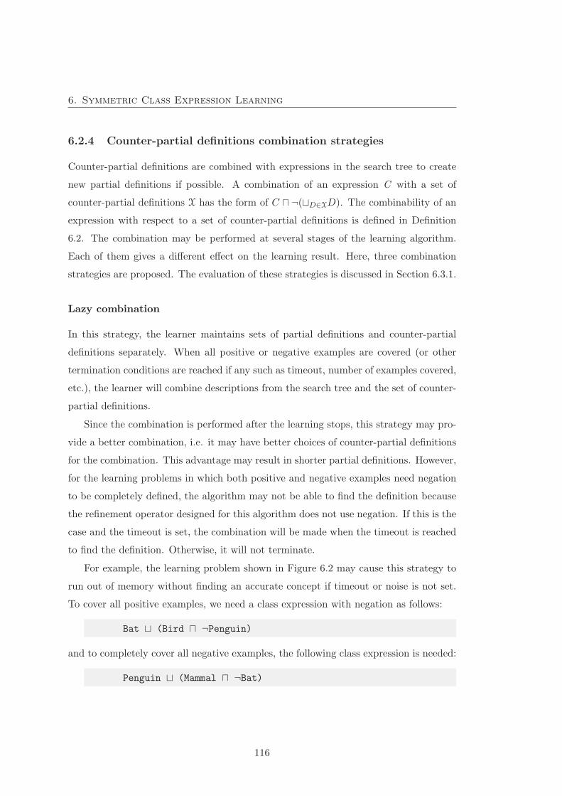
6. Symmetric Class Expression Learning
6.2.4 Counter-partial definitions combination strategies
Counter-partial definitions are combined with expressions in the search tree to create
new partial definitions if possible. A combination of an expression C with a set of
counter-partial definitions X has the form of C � ¬(�D∈XD). The combinability of an
expression with respect to a set of counter-partial definitions is defined in Definition
6.2. The combination may be performed at several stages of the learning algorithm.
Each of them gives a different effect on the learning result. Here, three combination
strategies are proposed. The evaluation of these strategies is discussed in Section 6.3.1.
Lazy combination
In this strategy, the learner maintains sets of partial definitions and counter-partial
definitions separately. When all positive or negative examples are covered (or other
termination conditions are reached if any such as timeout, number of examples covered,
etc.), the learner will combine descriptions from the search tree and the set of counter-
partial definitions.
Since the combination is performed after the learning stops, this strategy may pro-
vide a better combination, i.e. it may have better choices of counter-partial definitions
for the combination. This advantage may result in shorter partial definitions. However,
for the learning problems in which both positive and negative examples need negation
to be completely defined, the algorithm may not be able to find the definition because
the refinement operator designed for this algorithm does not use negation. If this is the
case and the timeout is set, the combination will be made when the timeout is reached
to find the definition. Otherwise, it will not terminate.
For example, the learning problem shown in Figure 6.2 may cause this strategy to
run out of memory without finding an accurate concept if timeout or noise is not set.
To cover all positive examples, we need a class expression with negation as follows:
Bat � (Bird � ¬Penguin)
and to completely cover all negative examples, the following class expression is needed:
Penguin � (Mammal � ¬Bat)
116
6. Symmetric Class Expression Learning
To produce the definition for positive examples, the counter-partial definition Penguin
is needed to combine with the expression Bird. This expression cannot be produced
directly by the refinement due to the removal of negation from the refinement operator.
However, in this strategy, the combination is only called when all positive examples or
negative examples are covered. Therefore, in this case, the combination can only be
called when all negative examples are covered. Unfortunately, this condition is never
met as the expression ¬Bat cannot be produced due to the removal of negation from
the refinement operator.
On-the-fly combination
This strategy is used in Algorithm 6.1. In this strategy, when a new description is gen-
erated from the refinement or an existing description is revisited (e.g. for refinement),
it is combined with the existing counter-partial definitions if possible. Practically, the
combination is performed on the worker side as new descriptions are always generated
by workers. This strategy can avoid the termination problem discussed in the lazy
combination strategy because negation is used in the combination which is performed
for every new description. The evaluation suggests that this strategy, overall, gives
the best performance and the smallest search tree. However, the final result should be
optimised, as a counter-partial definition can be combined with many expressions and
thus the final definition is unnecessary long.
For example, in the learning problem described in Figure 6.2, when description Bird
is generated, there is no counter-partial definition to combine with. However, when it
is revisited for refinement, it will be combined with the new counter-partial definition
Penguin to produce a partial definition Bird � ¬Penguin. Therefore, it can avoid the
termination problem that occurs when the lazy combination strategy is used.
Delayed combination
This is an intermediate solution between the above strategies that checks the possibility
of combinations when a new description is generated. However, even if the combination
is possible, only the set of cumulative covered positive examples is updated (by removing
from this set the elements that are covered by the new description), while the new
117
6. Symmetric Class Expression Learning
description is put into a potential partial definitions set. The combination is executed
when the termination condition is reached, i.e. either all positive examples or all
negative examples are covered, or the timeout is approached.
This strategy may help to prevent the problem of the lazy combination strategy. In
addition, it may return better combinations in comparison with the on-the-fly strategy
because it inherits the advantage of the lazy combination strategy. However, as the
combinable descriptions in this strategy are not combined until the learning terminates,
they can be refined and therefore the search tree is likely to be bigger than that of the
on-the-fly strategy.
6.3 Evaluation
The Symmetric Class Expression Learning approach was evaluated by four experiments
using the 10-fold cross-validation method and the datasets described in Chapter 3. The
first experiment was to investigate the effect of combination strategies on the search
tree size and predictive accuracy. The results from this experiment was the basic to
select the default combination strategy used with SPaCEL in further experiments. The
second experiment was to measure the search tree size generated by three algorithms on
each learning problem. In the third experiment, the predictive accuracy and learning
time of the three algorithms was computed. Finally, the length of the learnt definitions
produced by the three algorithms were examined in the fourth experiment.
The results of each experiment (except the first experiment, which uses only some
learning problems) in this chapter are divided into three groups. The first group in-
cludes the results of the 7 low to medium complexity learning problems. All learning
algorithms can find an accurate definition on the training set (i.e. without timeout) of
these datasets. The second group includes the results of 3 high to very high complexity
learning problems for which all learning algorithms can find accurate definitions of the
training set (i.e. without timeout). Finally, the third group contains the 6 remaining
learning problems, i.e. the learning problems for which at least one of the learning
algorithms could not find an accurate definition on the training set, i.e. a timeout oc-
curred. The reason for treating problems in this group separately is that some metrics
118
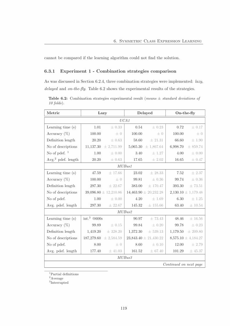
6. Symmetric Class Expression Learning
cannot be compared if the learning algorithm could not find the solution.
6.3.1 Experiment 1 - Combination strategies comparison
As was discussed in Section 6.2.4, three combination strategies were implemented: lazy,
delayed and on-the-fly. Table 6.2 shows the experimental results of the strategies.
Table 6.2: Combination strategies experimental result (means ± standard deviations of10 folds).
Metric Lazy Delayed On-the-fly
UCA1
Learning time (s) 1.01 ± 0.33 0.54 ± 0.23 0.72 ± 0.17
Accuracy (%) 100.00 ± 0 100.00 ± 0 100.00 ± 0
Definition length 20.20 ± 0.63 58.60 ± 21.31 66.60 ± 1.90
No of descriptions 11,137.30 ± 2,711.99 5,065.30 ± 1,867.64 6,998.70 ± 859.74
No of pdef. 1 1.00 ± 0.00 3.40 ± 1.27 4.00 ± 0.00
Avg.2 pdef. length 20.20 ± 0.63 17.65 ± 2.02 16.65 ± 0.47
MUBus1
Learning time (s) 47.59 ± 17.66 23.02 ± 28.33 7.52 ± 2.37
Accuracy (%) 100.00 ± 0 99.81 ± 0.36 99.74 ± 0.36
Definition length 297.30 ± 22.67 383.00 ± 170.47 393.30 ± 73.51
No of descriptions 39,096.80 ± 12,210.86 14,463.90 ± 20,232.28 2,130.10 ± 1,179.48
No of pdef. 1.00 ± 0.00 4.20 ± 1.69 6.30 ± 1.25
Avg. pdef. length 297.30 ± 22.67 145.32 ± 155.66 63.40 ± 10.54
MUBus2
Learning time (s) int.3 @600s 90.97 ± 73.43 48.46 ± 16.56
Accuracy (%) 99.89 ± 0.15 99.84 ± 0.20 99.78 ± 0.23
Definition length 1,419.20 ± 328.20 1,372.30 ± 539.13 1,179.50 ± 209.80
No of descriptions 187,279.60 ± 2,584.59 23,843.40 ± 21,430.22 8,575.10 ± 4,184.27
No of pdef. 8.00 ± 0 8.60 ± 0.10 12.00 ± 2.79
Avg. pdef. length 177.40 ± 41.03 161.52 ± 67.40 101.29 ± 45.37
MUBus3
Continued on next page
1Partial definitions2Average3Interrupted
119
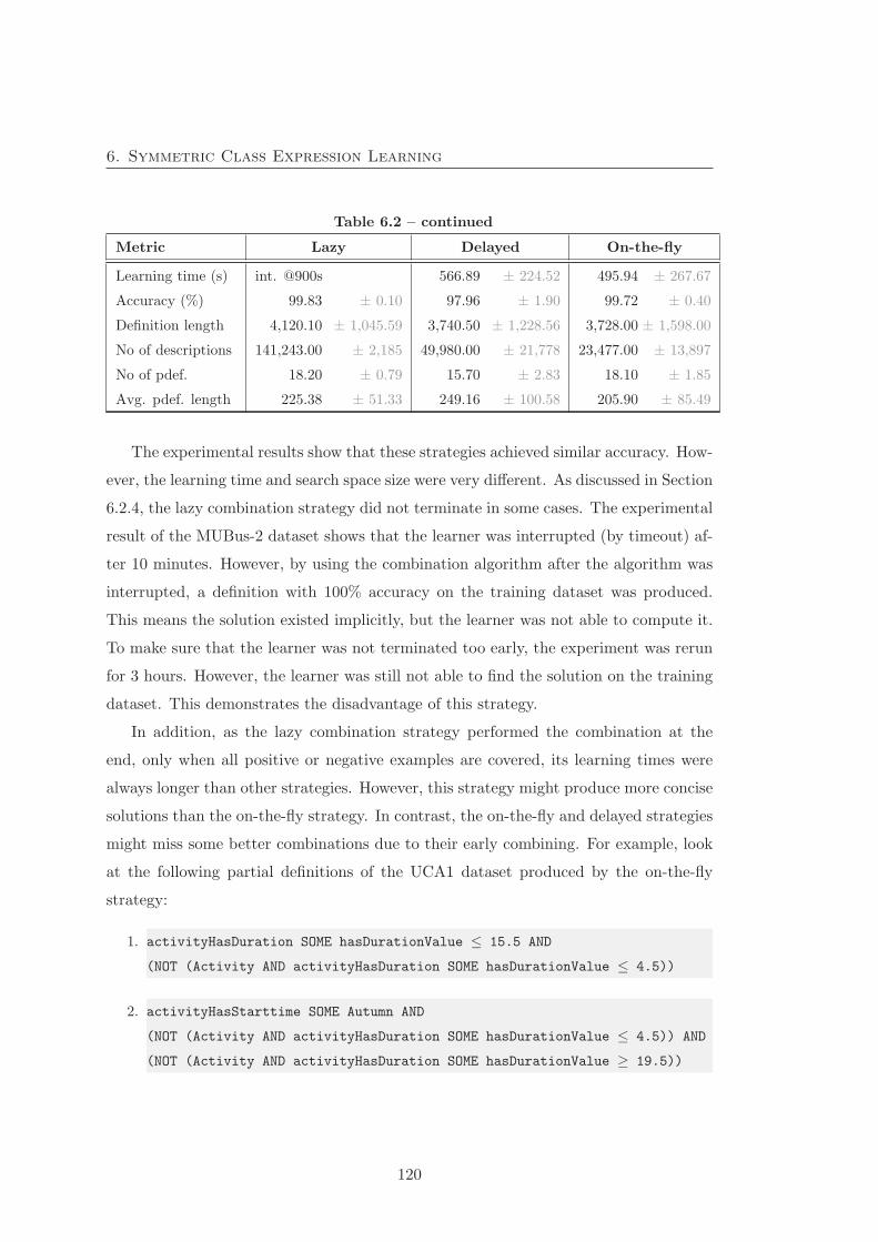
6. Symmetric Class Expression Learning
Table 6.2 – continued
Metric Lazy Delayed On-the-fly
Learning time (s) int. @900s 566.89 ± 224.52 495.94 ± 267.67
Accuracy (%) 99.83 ± 0.10 97.96 ± 1.90 99.72 ± 0.40
Definition length 4,120.10 ± 1,045.59 3,740.50 ± 1,228.56 3,728.00 ± 1,598.00
No of descriptions 141,243.00 ± 2,185 49,980.00 ± 21,778 23,477.00 ± 13,897
No of pdef. 18.20 ± 0.79 15.70 ± 2.83 18.10 ± 1.85
Avg. pdef. length 225.38 ± 51.33 249.16 ± 100.58 205.90 ± 85.49
The experimental results show that these strategies achieved similar accuracy. How-
ever, the learning time and search space size were very different. As discussed in Section
6.2.4, the lazy combination strategy did not terminate in some cases. The experimental
result of the MUBus-2 dataset shows that the learner was interrupted (by timeout) af-
ter 10 minutes. However, by using the combination algorithm after the algorithm was
interrupted, a definition with 100% accuracy on the training dataset was produced.
This means the solution existed implicitly, but the learner was not able to compute it.
To make sure that the learner was not terminated too early, the experiment was rerun
for 3 hours. However, the learner was still not able to find the solution on the training
dataset. This demonstrates the disadvantage of this strategy.
In addition, as the lazy combination strategy performed the combination at the
end, only when all positive or negative examples are covered, its learning times were
always longer than other strategies. However, this strategy might produce more concise
solutions than the on-the-fly strategy. In contrast, the on-the-fly and delayed strategies
might miss some better combinations due to their early combining. For example, look
at the following partial definitions of the UCA1 dataset produced by the on-the-fly
strategy:
1. activityHasDuration SOME hasDurationValue ≤ 15.5 AND
(NOT (Activity AND activityHasDuration SOME hasDurationValue ≤ 4.5))
2. activityHasStarttime SOME Autumn AND
(NOT (Activity AND activityHasDuration SOME hasDurationValue ≤ 4.5)) AND
(NOT (Activity AND activityHasDuration SOME hasDurationValue ≥ 19.5))
120

6. Symmetric Class Expression Learning
3. activityHasStarttime SOME Summer AND
(NOT (Activity AND activityHasDuration SOME hasDurationValue ≤ 4.5)) AND
(NOT (Activity AND activityHasDuration SOME hasDurationValue ≥ 19.5))
4. activityHasDuration SOME hasDurationValue ≥ 4.5 AND
activityHasStarttime SOME Spring AND
(NOT (Activity AND activityHasDuration SOME hasDurationValue ≥ 19.5))
and by the delayed strategy:
activityHasDuration SOME (hasDurationValue ≥ 4.5 AND
hasDurationValue ≤ 19.5) AND
(NOT (activityHasStarttime SOME Winter AND activityHasDuration SOME
hasDurationValue ≥ 15.5))
The partial definitions produced by the on-the-fly strategy consist of a larger number
of short expressions and counter-partial definitions (length is from 5 to 7) while partial
definitions produced by the lazy strategy consisted of a small number of long counter-
partial definitions (length is 9). Therefore, the final definitions produced by the on-the-
fly strategy were usually longer than the definitions produced by the delayed strategy.
However, one of the weak points of the lazy strategy is that it might not achieve an
accurate solution even if a solution exists. The different combination strategies all have
different trade-offs between definition length and learning time.
The on-the-fly strategy produced promising results. It dominated other strategies
in most aspects, especially the learning time and the number of descriptions (search
space). There was only one exception in the dataset MUBus-1, where this strategy
produced a longer definition than others. The number of partial definitions involved
in the solution can help to explain the difference: there were common parts (counter-
partial definitions) amongst the partial definitions.
Finally, the delayed combination strategy was better than the lazy evaluation strat-
egy, but worse than the on-the-fly strategy, on the learning time and the number of
descriptions. This strategy was expected to get the advantages of both on-the-fly and
lazy strategies to produce shorter definitions than the lazy strategy and use smaller
search spaces than the on-the-fly strategy. However, the experimental results showed
121

6. Symmetric Class Expression Learning
that this idea did not help much. The definitions produced by the delayed strategy
were not always shorter than the definitions produced by the lazy strategy while the
search spaces were always bigger. Therefore, the on-the-fly was chosen as the major
combination strategy for the SPaCEL algorithm to compare with other learners in the
evaluation.
6.3.2 Experiment 2 - Search tree size comparison
The search tree size reported in this experiment is the total number of all descriptions
that are inserted into the search tree, including the irrelevant descriptions (the partial
and counter-partial definitions which are removed later by the algorithm). If an algo-
rithm can find the solution, the result reported is the search tree size after the learning
algorithm has terminated. Otherwise, it is the search tree size at the moment when the
timeout has occurred. In this case, the comparison should be treated with caution as
it depends upon the timeout assigned for the learning algorithm.
The search tree size generated by the three algorithms on the evaluation datasets
is shown in Table 6.3. In this experiment, only learning problems on which at least
one of the algorithms found an accurate definition on the training set were considered.
The comparison cannot be made if all three learning algorithms time out. Therefore,
the results for the CarcinoGenesis and ILDP learning problems are not reported.
In the first group of learning problems, SPaCEL had smaller search trees than both
CELOE and ParCEL for 4/7 learning problems and smaller than one of them in the
remaining 3 learning problems. However, this group might not reflect well the reduction
of the search tree size by our approach as it contains low to medium complexity prob-
lems. The definitions of these learning problems were short and therefore the search
tree sizes were usually small. Consequently, they were sensitive to the parallelisation.
In detail, as the search tree in our algorithm is expanded by multiple workers, the so-
lution may be found by one of the workers while the other workers are still processing
the search tree. Consequently, the search tree may be expanded redundantly and thus
the reported search tree sizes might be unnecessarily larger than the minimal search
tree size required to learn the problem.
In the second and the third groups, SPaCEL always produced the smallest search
122
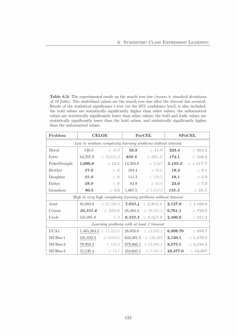
6. Symmetric Class Expression Learning
Table 6.3: The experimental result on the search tree size (means ± standard deviationsof 10 folds). The underlined values are the search tree size after the timeout has occured.Result of the statistical significance t-test (at the 95% confidence level) is also included:the bold values are statistically significantly higher than other values; the unformattedvalues are statistically significantly lower than other values; the bold and italic values arestatistically significantly lower than the bold values, and statistically significantly higherthan the unformatted values.
Problem CELOE ParCEL SPaCEL
Low to medium complexity learning problems without timeout
Moral 540.5 ± 16.9 33.3 ± 11.0 223.4 ± 364.2
Forte 64,707.9 ± 33,641.9 859.5 ± 251.2 174.1 ± 108.2
PokerStraight 1,090.8 ± 12.5 14,204.8 ± 2,847 2,105.0 ± 1,217.7
Brother 37.0 ± 0 104.4 ± 92.6 18.4 ± 9.1
Daughter 21.0 ± 0 111.3 ± 110.2 18.1 ± 5.9
Father 29.0 ± 0 82.9 ± 63.8 23.0 ± 7.0
Grandson 80.5 ± 3.0 1,867.5 ± 1,519.3 125.3 ± 25.3
High to very high complexity learning problems without timeout
Aunt 85,883.8 ± 67,328.8 7,023.4 ± 2,912.1 2,127.8 ± 1,160.9
Cousin 20,331.6 ± 233.6 35,484.4 ± 39,055.4 6,761.1 ± 722.9
Uncle 541,081.8 ± 0 6,332.5 ± 3,247.9 2,400.0 ± 551.2
Learning problems with at least 1 timeout
UCA1 1,465,263.2 ± 11,515.5 28,676.0 ± 14,935.2 6,998.70 ± 859.7
MUBus-1 161,832.2 ± 3,054.5 643,401.5 ± 139,303 2,130.1 ± 1,179.5
MUBus-2 79.959.2 ± 118.5 879,866.1 ± 34,000.4 8,575.1 ± 4,184.3
MUBus-3 55,130.4 ± 73.7 453,605.1 ± 7,565.3 23,477.0 ± 13,897
123

6. Symmetric Class Expression Learning
trees for all learning problems in comparison with CELOE and ParCEL. The search
tree sizes generated by the three algorithms for the same learning problem in this
group were extremely different. For examples, SPaCEL only needed to explore about
2,400 expressions to find the solution for the Uncle learning problem while CELOE had
to explore more than 541,081 expressions. Similarly, SPaCEL found a solution after
exploring about 2,130 expressions while ParCEL needed to explore 643,401 expressions
on the MUBus-1 learning problem. CELOE could not find an accurate solution for this
learning problem and timed out after 10 minutes. The average search tree size at the
time of timeout was about 161,832 expressions.
A t-test rejected the null hypothesis for all learning problems at the 99% confidence
level. That means all differences between search tree sizes generated by three algorithms
on each dataset were statistically significant at the 1% significance level. Therefore, the
search trees generated by SPaCEL were statistically significantly smaller than CELOE
in 12/14 learning problems and than ParCEL for 13/14 learning problems.
6.3.3 Experiment 3 - Predictive accuracy and learning time
In this experiment, the predictive accuracy and learning time of the three learning
algorithms on the evaluation datasets were measured and compared. The experimental
results are shown in Table 6.4.
Table 6.4: Learning time and predictive accuracy experimental results summary (means± standard deviations of 10 folds). Result of the statistical significance t-test (at the 95%confidence level) is also included: the bold and highlighted values are statistically signifi-cantly better than other values; the unformatted values are statistically significantly worsethan other values; the bold and italic and highlighted values are statistically significantlyworse than the bold and highlighted values, and statistically significantly better than theunformatted values; the underlined values represent the values that are not statisticallysignificantly different from the other values.
Problem Predictive accuracy (%) Learning time (s)
CELOE ParCEL SPaCEL CELOE ParCEL SPaCEL
Low to medium complexity learning problems without timeout.
Moral 100.00
±0.00
100.00
±0.00
100.00
±0.00
0.15
±0.03
0.02
±0.01
0.03
±0.02
Continued on next page
124
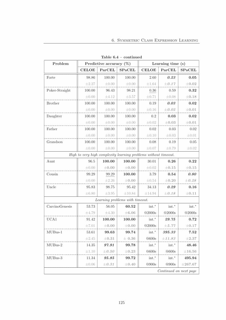
6. Symmetric Class Expression Learning
Table 6.4 – continued
Problem Predictive accuracy (%) Learning time (s)
CELOE ParCEL SPaCEL CELOE ParCEL SPaCEL
Forte 98.86
±2.27
100.00
±0.00
100.00
±0.00
2.60
±1.64
0.23
±0.17
0.05
±0.02
Poker-Straight 100.00
±0.00
96.43
±4.12
98.21
±3.57
0.36
±0.71
0.59
±0.08
0.32
±0.18
Brother 100.00
±0.00
100.00
±0.00
100.00
±0.00
0.19
±0.16
0.03
±0.02
0.02
±0.01
Daughter 100.00
±0.00
100.00
±0.00
100.00
±0.00
0.2
±0.02
0.03
±0.03
0.02
±0.01
Father 100.00
±0.00
100.00
±0.00
100.00
±0.00
0.02
±0.10
0.03
±0.03
0.02
±0.01
Grandson 100.00
±0.00
100.00
±0.00
100.00
±0.00
0.08
±0.07
0.19
±0.79
0.05
±0.02
High to very high complexity learning problems without timeout.
Aunt 96.5
±0.00
100.00
±0.00
100.00
±0.00
30.01
±0.02
0.26
±0.15
0.22
±0.15
Cousin 99.29
±0.00
99.29
±2.26
100.00
±0.00
3.79
±0.54
0.54
±0.20
0.80
±0.28
Uncle 95.83
±6.80
98.75
±3.95
95.42
±10.84
34.13
±14.94
0.29
±0.18
0.16
±0.11
Learning problems with timeout.
CarcinoGenesis 53.73
±4.79
56.05
±4.30
60.52
±6.06
int.∗
@2000s
int.∗
@2000s
int.∗
@2000s
UCA1 91.42
±7.01
100.00
±0.00
100.00
±0.00
int.∗
@2000s
29.75
±5.77
0.72
±0.17
MUBus-1 53.61
±2.45
99.63
±0.31
99.74
± 0.36
int.∗
@600s
395.33
±11.83
7.52
±2.37
MUBus-2 14.35
±1.10
97.91
±0.50
99.78
±0.23
int.∗
@600s
int.∗
@600s
48.46
±16.56
MUBus-3 11.34
±0.06
95.85
±0.31
99.72
±0.40
int.∗
@900s
int.∗
@900s
495.94
±267.67
Continued on next page
125
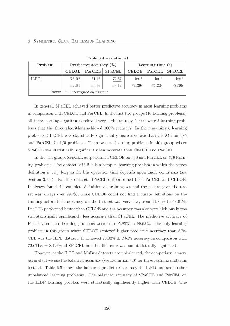
6. Symmetric Class Expression Learning
Table 6.4 – continued
Problem Predictive accuracy (%) Learning time (s)
CELOE ParCEL SPaCEL CELOE ParCEL SPaCEL
ILPD 76.02
±2.61
71.12
±5.36
72.67
±8.12
int.∗
@120s
int.∗
@120s
int.∗
@120s
Note: ∗: Interrupted by timeout
In general, SPaCEL achieved better predictive accuracy in most learning problems
in comparison with CELOE and ParCEL. In the first two groups (10 learning problems)
all three learning algorithms archived very high accuracy. There were 5 learning prob-
lems that the three algorithms achieved 100% accuracy. In the remaining 5 learning
problems, SPaCEL was statistically significantly more accurate than CELOE for 3/5
and ParCEL for 1/5 problems. There was no learning problems in this group where
SPaCEL was statistically significantly less accurate than CELOE and ParCEL.
In the last group, SPaCEL outperformed CELOE on 5/6 and ParCEL on 3/6 learn-
ing problems. The dataset MU-Bus is a complex learning problem in which the target
definition is very long as the bus operation time depends upon many conditions (see
Section 3.3.3). For this dataset, SPaCEL outperformed both ParCEL and CELOE.
It always found the complete definition on training set and the accuracy on the test
set was always over 99.7%, while CELOE could not find accurate definitions on the
training set and the accuracy on the test set was very low, from 11.34% to 53.61%.
ParCEL performed better than CELOE and the accuracy was also very high but it was
still statistically significantly less accurate than SPaCEL. The predictive accuracy of
ParCEL on these learning problems were from 95.85% to 99.63%. The only learning
problem in this group where CELOE achieved higher predictive accuracy than SPa-
CEL was the ILPD dataset. It achieved 76.02% ± 2.61% accuracy in comparison with
72.671% ± 8.123% of SPaCEL but the difference was not statistically significant.
However, as the ILPD and MuBus datasets are unbalanced, the comparison is more
accurate if we use the balanced accuracy (see Definition 5.6) for these learning problems
instead. Table 6.5 shows the balanced predictive accuracy for ILPD and some other
unbalanced learning problems. The balanced accuracy of SPaCEL and ParCEL on
the ILDP learning problem were statistically significantly higher than CELOE. The
126
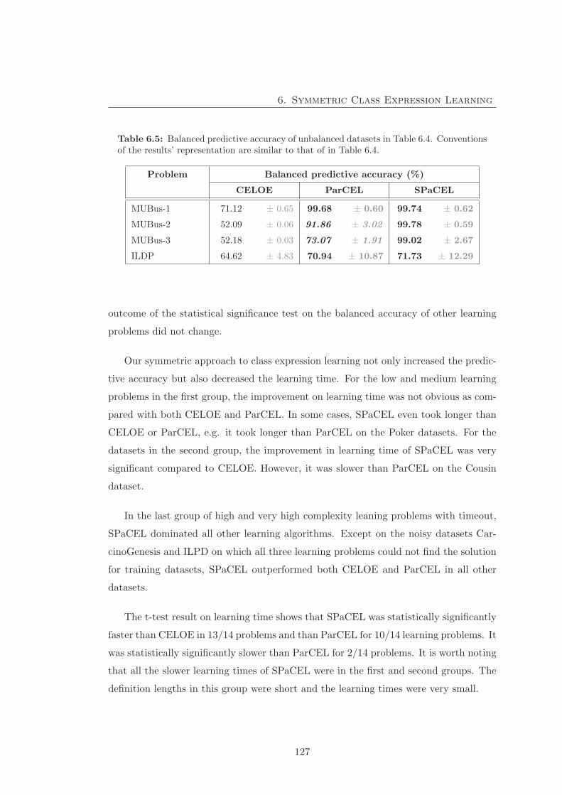
6. Symmetric Class Expression Learning
Table 6.5: Balanced predictive accuracy of unbalanced datasets in Table 6.4. Conventionsof the results’ representation are similar to that of in Table 6.4.
Problem Balanced predictive accuracy (%)
CELOE ParCEL SPaCEL
MUBus-1 71.12 ± 0.65 99.68 ± 0.60 99.74 ± 0.62
MUBus-2 52.09 ± 0.06 91.86 ± 3.02 99.78 ± 0.59
MUBus-3 52.18 ± 0.03 73.07 ± 1.91 99.02 ± 2.67
ILDP 64.62 ± 4.83 70.94 ± 10.87 71.73 ± 12.29
outcome of the statistical significance test on the balanced accuracy of other learning
problems did not change.
Our symmetric approach to class expression learning not only increased the predic-
tive accuracy but also decreased the learning time. For the low and medium learning
problems in the first group, the improvement on learning time was not obvious as com-
pared with both CELOE and ParCEL. In some cases, SPaCEL even took longer than
CELOE or ParCEL, e.g. it took longer than ParCEL on the Poker datasets. For the
datasets in the second group, the improvement in learning time of SPaCEL was very
significant compared to CELOE. However, it was slower than ParCEL on the Cousin
dataset.
In the last group of high and very high complexity leaning problems with timeout,
SPaCEL dominated all other learning algorithms. Except on the noisy datasets Car-
cinoGenesis and ILPD on which all three learning problems could not find the solution
for training datasets, SPaCEL outperformed both CELOE and ParCEL in all other
datasets.
The t-test result on learning time shows that SPaCEL was statistically significantly
faster than CELOE in 13/14 problems and than ParCEL for 10/14 learning problems. It
was statistically significantly slower than ParCEL for 2/14 problems. It is worth noting
that all the slower learning times of SPaCEL were in the first and second groups. The
definition lengths in this group were short and the learning times were very small.
127
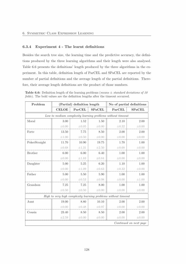
6. Symmetric Class Expression Learning
6.3.4 Experiment 4 - The learnt definitions
Besides the search tree size, the learning time and the predictive accuracy, the defini-
tions produced by the three learning algorithms and their length were also analysed.
Table 6.6 presents the definitions’ length produced by the three algorithms in the ex-
periment. In this table, definition length of ParCEL and SPaCEL are reported by the
number of partial definitions and the average length of the partial definitions. There-
fore, their average length definitions are the product of those numbers.
Table 6.6: Definition length of the learning problems (means ± standard deviations of 10folds). The bold values are the definition lengths after the timeout occurred.
Problem (Partial) definition length No of partial definitions
CELOE ParCEL SPaCEL ParCEL SPaCEL
Low to medium complexity learning problems without timeout
Moral 3.00
±0.00
1.52
±0.05
1.50
±0.00
2.10
±0.32
2.00
±0.00
Forte 13.50
±1.00
7.75
±0.50
8.50
±0.00
2.00
±0.00
2.00
±0.00
PokerStraight 11.70
±0.68
10.90
±1.31
19.75
±2.50
1.70
±0.68
1.00
±0.00
Brother 6.00
±0.00
6.00
±1.83
6.40
±0.84
1.00
±0.00
1.00
±0.00
Daughter 5.00
±0.00
5.25
±1.09
6.20
±0.63
1.10
±0.32
1.00
±0.00
Father 5.00
±0.00
5.50
±0.53
5.90
±0.98
1.00
±0.00
1.00
±1.00
Grandson 7.25
±0.50
7.25
±0.50
8.00
±0.00
1.00
±0.00
1.00
±0.00
High to very high complexity learning problems without timeout
Aunt 19.00
±0.00
8.80
±0.48
10.10
±0.97
2.00
±0.00
2.00
±0.00
Cousin 23.40
±2.59
8.50
±0.00
8.50
±0.00
2.00
±0.00
2.00
±0.00
Continued on next page
128
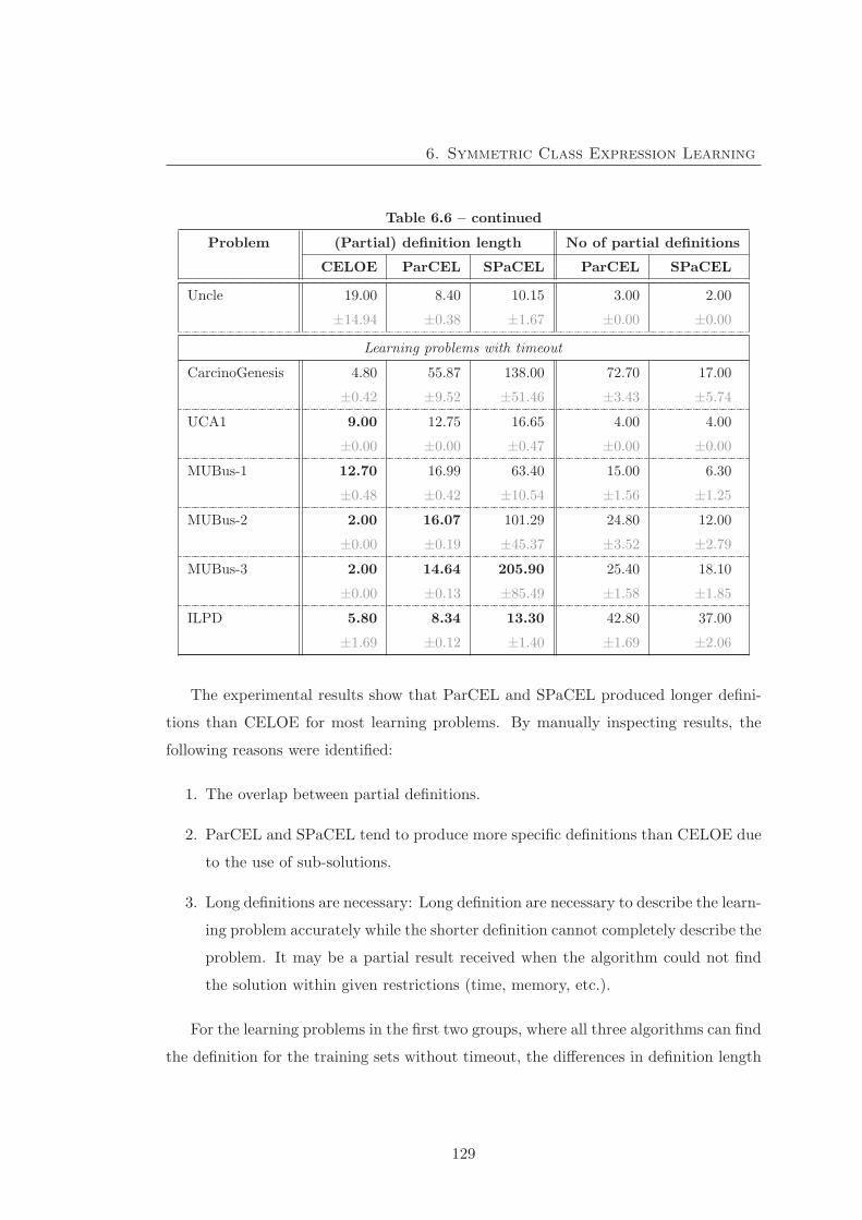
6. Symmetric Class Expression Learning
Table 6.6 – continued
Problem (Partial) definition length No of partial definitions
CELOE ParCEL SPaCEL ParCEL SPaCEL
Uncle 19.00
±14.94
8.40
±0.38
10.15
±1.67
3.00
±0.00
2.00
±0.00
Learning problems with timeout
CarcinoGenesis 4.80
±0.42
55.87
±9.52
138.00
±51.46
72.70
±3.43
17.00
±5.74
UCA1 9.00
±0.00
12.75
±0.00
16.65
±0.47
4.00
±0.00
4.00
±0.00
MUBus-1 12.70
±0.48
16.99
±0.42
63.40
±10.54
15.00
±1.56
6.30
±1.25
MUBus-2 2.00
±0.00
16.07
±0.19
101.29
±45.37
24.80
±3.52
12.00
±2.79
MUBus-3 2.00
±0.00
14.64
±0.13
205.90
±85.49
25.40
±1.58
18.10
±1.85
ILPD 5.80
±1.69
8.34
±0.12
13.30
±1.40
42.80
±1.69
37.00
±2.06
The experimental results show that ParCEL and SPaCEL produced longer defini-
tions than CELOE for most learning problems. By manually inspecting results, the
following reasons were identified:
1. The overlap between partial definitions.
2. ParCEL and SPaCEL tend to produce more specific definitions than CELOE due
to the use of sub-solutions.
3. Long definitions are necessary: Long definition are necessary to describe the learn-
ing problem accurately while the shorter definition cannot completely describe the
problem. It may be a partial result received when the algorithm could not find
the solution within given restrictions (time, memory, etc.).
For the learning problems in the first two groups, where all three algorithms can find
the definition for the training sets without timeout, the differences in definition length
129

6. Symmetric Class Expression Learning
between three algorithms were small. This was caused by the overlap between partial
definitions. In some cases, they can be shortened using some optimisation strategies.
For example, the definitions produced by CELOE and SPaCEL for the Forte dataset
(the uncle relationship definition) are:
• CELOE:
male AND ((married SOME sibling SOME Person) OR
(married SOME hasSibling SOME hasChild SOME Thing))
• SPaCEL (two partial definitions):
1. hasSibling SOME hasChild SOME Thing AND (NOT female)
2. married SOME hasSibling SOME hasChild SOME Thing AND (NOT female)
The length of the definition produced by CELOE is 15 and SPaCEL is 19 (length
of two partial definitions plus 1 for disjunction). However, at least 3 axioms in the
SPaCEL final definition can be reduced by removing the common part among partial
definitions, i.e. AND NOT female. That means if the same normal form [51, 86] is
applied for both CELOE and SPaCEL, the difference between their lengths can be
reduced. Moreover, NOT female can be replaced by Male if male and female are
declared as disjoint properties. This is the idea of the optimisation and simplification
in description logic [3, 65]. Currently, this idea has not yet been implemented in
our algorithm. However, breaking down a long definition (as for CELOE) into several
smaller partial definitions (as for SPaCEL) may help the definitions to be more readable,
particularly for long definitions.
For the learning problems on which at least one of the learning algorithms cannot
find an accurate definition on the training set, i.e. the timeout occurred in the exper-
iments, definitions produced by SPaCEL are significant longer than those of CELOE.
In some learning problems, CELOE produced shorter definitions because it could not
find the solution for the training set. This is also the major class of learning problem
that we want to focus on, i.e. complex learning problems. The experimental result
on the UCA1 dataset is used to demonstrate the difference in searching for the defini-
tions between the three algorithms. This is a complex and noiseless learning problem.
130
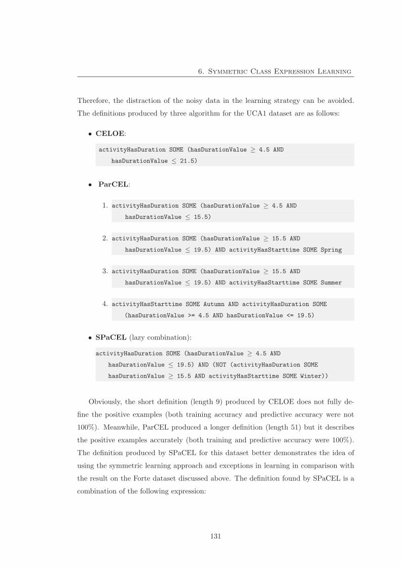
6. Symmetric Class Expression Learning
Therefore, the distraction of the noisy data in the learning strategy can be avoided.
The definitions produced by three algorithm for the UCA1 dataset are as follows:
• CELOE:
activityHasDuration SOME (hasDurationValue ≥ 4.5 AND
hasDurationValue ≤ 21.5)
• ParCEL:
1. activityHasDuration SOME (hasDurationValue ≥ 4.5 AND
hasDurationValue ≤ 15.5)
2. activityHasDuration SOME (hasDurationValue ≥ 15.5 AND
hasDurationValue ≤ 19.5) AND activityHasStarttime SOME Spring
3. activityHasDuration SOME (hasDurationValue ≥ 15.5 AND
hasDurationValue ≤ 19.5) AND activityHasStarttime SOME Summer
4. activityHasStarttime SOME Autumn AND activityHasDuration SOME
(hasDurationValue >= 4.5 AND hasDurationValue <= 19.5)
• SPaCEL (lazy combination):
activityHasDuration SOME (hasDurationValue ≥ 4.5 AND
hasDurationValue ≤ 19.5) AND (NOT (activityHasDuration SOME
hasDurationValue ≥ 15.5 AND activityHasStarttime SOME Winter))
Obviously, the short definition (length 9) produced by CELOE does not fully de-
fine the positive examples (both training accuracy and predictive accuracy were not
100%). Meanwhile, ParCEL produced a longer definition (length 51) but it describes
the positive examples accurately (both training and predictive accuracy were 100%).
The definition produced by SPaCEL for this dataset better demonstrates the idea of
using the symmetric learning approach and exceptions in learning in comparison with
the result on the Forte dataset discussed above. The definition found by SPaCEL is a
combination of the following expression:
131
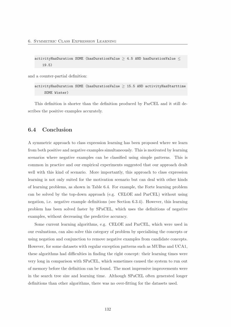
6. Symmetric Class Expression Learning
activityHasDuration SOME (hasDurationValue ≥ 4.5 AND hasDurationValue ≤19.5)
and a counter-partial definition:
activityHasDuration SOME (hasDurationValue ≥ 15.5 AND activityHasStarttime
SOME Winter)
This definition is shorter than the definition produced by ParCEL and it still de-
scribes the positive examples accurately.
6.4 Conclusion
A symmetric approach to class expression learning has been proposed where we learn
from both positive and negative examples simultaneously. This is motivated by learning
scenarios where negative examples can be classified using simple patterns. This is
common in practice and our empirical experiments suggested that our approach dealt
well with this kind of scenario. More importantly, this approach to class expression
learning is not only suited for the motivation scenario but can deal with other kinds
of learning problems, as shown in Table 6.4. For example, the Forte learning problem
can be solved by the top-down approach (e.g. CELOE and ParCEL) without using
negation, i.e. negative example definitions (see Section 6.3.4). However, this learning
problem has been solved faster by SPaCEL, which uses the definitions of negative
examples, without decreasing the predictive accuracy.
Some current learning algorithms, e.g. CELOE and ParCEL, which were used in
our evaluations, can also solve this category of problem by specialising the concepts or
using negation and conjunction to remove negative examples from candidate concepts.
However, for some datasets with regular exception patterns such as MUBus and UCA1,
these algorithms had difficulties in finding the right concept: their learning times were
very long in comparison with SPaCEL, which sometimes caused the system to run out
of memory before the definition can be found. The most impressive improvements were
in the search tree size and learning time. Although SPaCEL often generated longer
definitions than other algorithms, there was no over-fitting for the datasets used.
132

6. Symmetric Class Expression Learning
However, the definitions generated by SPaCEL are not optimised. The normalisa-
tion and simplification can be used to produce better definitions, i.e. shorter and more
readable. This, together with the investigations on more datasets will be the future
work for further research.
133

6. Symmetric Class Expression Learning
134

Chapter 7
Improving Predictive Correctness
by Fortification
This chapter proposes a method to improve the predictive correctness of class
expression learning. The motivation for this is described first, followed by a
method for addressing the problem. Then, the architecture and algorithm for
the proposed method is introduced. The chapter ends with several experi-
ments to demonstrate the efficacy of the proposed method.
7.1 Problem Description
Predictive accuracy is the basic criteria used in assessment of the learnt concepts in
machine learning. It reflects the prediction ability of the learnt concepts over unseen
examples. Essentially, predictive accuracy of a learnt concept depends upon the number
of covered positive (true positives) and uncovered negative (true negatives) examples of
the learnt concept. These are the two main factors that directly affect the completeness
and correctness of the prediction (see Section 3.2.1 for details).
In description logic learning, the top-down approach is mostly used in comparison
with other approaches as it can use the rich hierarchical structure of the knowledge
base to build the search tree. This approach produces short, concise definitions and
135
7. Improving Predictive Correctness by Fortification
thus the learnt definitions tend to be biased towards generality, i.e. the completeness of
the prediction. This is suitable for some types of applications. However there are also
certain types of application that require bias towards the correctness of the prediction.
For example, consider the criminal behaviour warning systems that observe and
learn the usual patterns of the daily life activities and use them, along with the Negation
As Failure (NAF) inference rule [27, 40], to predict criminal activities. In these systems,
missing criminal behaviours is very serious. Therefore, suppose that the cry-wolf effect
[19, 22, 139] can be avoided, such systems usually prefer the false positives to the false
negatives. Similarly, consider the elderly care systems in which the systems also observe
and learn the normal behaviours of the elderly and use the learnt behaviours, together
with NAF inference rule, to detect abnormalities. Missing any abnormal behaviours
may threaten the inhabitant’s safety. In other words, correctness of the learnt rules
is more important than the completeness. It is worth noting that normal and legal
(moral) behaviours occur much more often than abnormal and criminal behaviours.
Therefore, learning the normal and moral behaviours will result in better descriptions
of the behaviours than that of the criminal or abnormal behaviours. Consequently, it
is more plausible to learn and use moral and normal behaviour patterns (with NAF)
to detect the criminal and abnormal behaviour than to learn and use the normal and
criminal or abnormal behaviour patterns.
Learning in description logics is essentially a search problem (see Section 2.2.2) and
most learning algorithms use a search heuristic to guide the search. A common method
for trading off between completeness and correctness of the learnt concepts is to adjust
the search heuristic [69, 70]. A learning algorithm that uses a search heuristic pri-
oritising completeness will likely produce higher completeness concepts than learning
algorithms that prioritise correctness and vice verse. However, an inappropriate ad-
justment to the search heuristic may prevent the learning algorithm from achieving the
right definition. Moreover, this approach is not flexible as changing the trade-off level
requires the learning problem to be relearnt. Therefore, in this chapter, an approach is
proposed to improve the predictive correctness for class expression learning algorithms
that can avoid the above problems. The basic idea of this method is to fortify the
learnt concept by a redundant specialisation to reduce the number of false positives. In
136
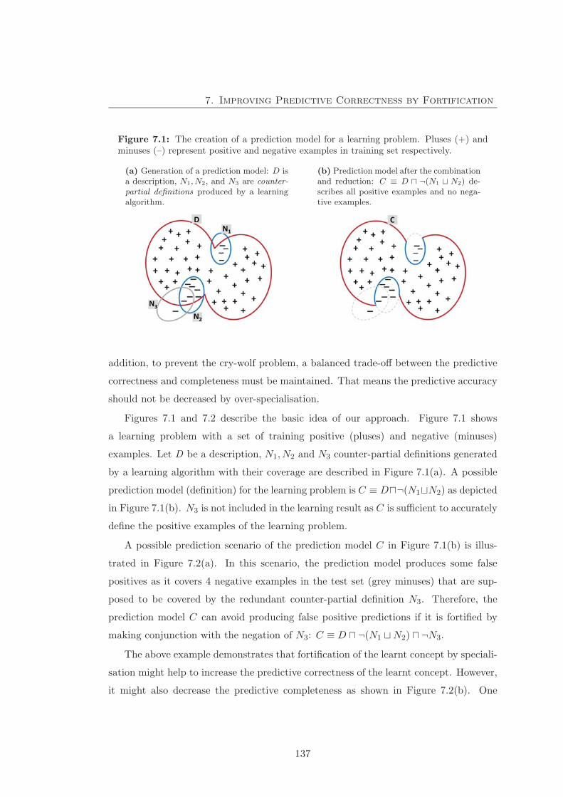
7. Improving Predictive Correctness by Fortification
Figure 7.1: The creation of a prediction model for a learning problem. Pluses (+) andminuses (–) represent positive and negative examples in training set respectively.
(a) Generation of a prediction model: D isa description, N1, N2, and N3 are counter-partial definitions produced by a learningalgorithm.
(b) Prediction model after the combinationand reduction: C ≡ D � ¬(N1 � N2) de-scribes all positive examples and no nega-tive examples.
addition, to prevent the cry-wolf problem, a balanced trade-off between the predictive
correctness and completeness must be maintained. That means the predictive accuracy
should not be decreased by over-specialisation.
Figures 7.1 and 7.2 describe the basic idea of our approach. Figure 7.1 shows
a learning problem with a set of training positive (pluses) and negative (minuses)
examples. Let D be a description, N1, N2 and N3 counter-partial definitions generated
by a learning algorithm with their coverage are described in Figure 7.1(a). A possible
prediction model (definition) for the learning problem is C ≡ D�¬(N1�N2) as depicted
in Figure 7.1(b). N3 is not included in the learning result as C is sufficient to accurately
define the positive examples of the learning problem.
A possible prediction scenario of the prediction model C in Figure 7.1(b) is illus-
trated in Figure 7.2(a). In this scenario, the prediction model produces some false
positives as it covers 4 negative examples in the test set (grey minuses) that are sup-
posed to be covered by the redundant counter-partial definition N3. Therefore, the
prediction model C can avoid producing false positive predictions if it is fortified by
making conjunction with the negation of N3: C ≡ D � ¬(N1 �N2) � ¬N3.
The above example demonstrates that fortification of the learnt concept by speciali-
sation might help to increase the predictive correctness of the learnt concept. However,
it might also decrease the predictive completeness as shown in Figure 7.2(b). One
137

7. Improving Predictive Correctness by Fortification
Figure 7.2: A prediction scenario of the prediction model in Figure 7.1. Grey pluses andminuses represent positive and negative examples in the prediction (test set).
(a) Prediction model without N3. Thereare 4 negative examples covered by C thatare also covered by N3. However, N3 wasremoved by reduction as it is redundant inthe training model.
(b) Prediction model with N3. If N3 isincluded in C, 4 covered negative examplesin Figure 7.2(a) can be removed from theC coverage. However, N3 also excludes onepositive example from C coverage.
more positive example is misclassified caused by the fortification. Moreover, inappro-
priate fortification not only cannot increase predictive correctness, but also decreases
predictive completeness. For example, Figure 7.3(a) shows a learning problem with 6
learnt descriptions. Three of them, D,N1 and N2, are sufficient to construct the final
definition. The remaining descriptions, N3, N4 and N5, are the potential candidates
for fortification of the learnt concept. However, the predictive model in Figure 7.3(b)
suggests that only N3 can help to increase predictive correctness and accuracy. On the
other hand, N4 does not change the prediction accuracy while N5 decrease predictive
completeness and accuracy.
Therefore, there are a number of challenges to improve the predictive correctness
using fortification, with the constraint on the balance trade-off between the predictive
correctness and predictive completeness, as follows:
Q1. How to generate candidates for fortification? Fortification candidates are descrip-
tions that can remove negative examples covered by the learnt concept in the test
set or more generally in the prediction (classification). The proposed method must
be general so that it can be used with most class expression learning algorithms.
Q2. How to choose the best candidates for fortification? As was described in Fig-
ure 7.3(b), fortification candidates may have different effects on the fortification.
138
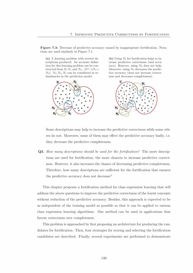
7. Improving Predictive Correctness by Fortification
Figure 7.3: Decrease of predictive accuracy caused by inappropriate fortification. Nota-tions are used similarly in Figure 7.1.
(a) A learning problem with several de-scriptions produced. An accurate defini-tion for this learning problem can be con-structed from D,N1 and N2 : D�¬(N1�N2). N3, N4, N5 can be considered as re-dundancies in the prediction model.
(b) Using N3 for fortification helps to in-crease predictive correctness (and accu-racy). However, using N4 does not help.Moreover, using N5 decreases the predic-tive accuracy (does not increase correct-ness and decreases completeness).
Some descriptions may help to increase the predictive correctness while some oth-
ers do not. Moreover, some of them may effect the predictive accuracy badly, i.e.
they decrease the predictive completeness.
Q3. How many descriptions should be used for the fortification? The more descrip-
tions are used for fortification, the more chances to increase predictive correct-
ness. However, it also increases the chance of decreasing predictive completeness.
Therefore, how many descriptions are sufficient for the fortification that ensures
the predictive accuracy does not decrease?
This chapter proposes a fortification method for class expression learning that will
address the above questions to improve the predictive correctness of the learnt concepts
without reduction of the predictive accuracy. Besides, this approach is expected to be
as independent of the training model as possible so that it can be applied to various
class expression learning algorithms. Our method can be used in applications that
favour correctness over completeness.
This problem is approached by first proposing an architecture for producing the can-
didates for fortification. Then, four strategies for scoring and selecting the fortification
candidates are described. Finally, several experiments are performed to demonstrate
139

7. Improving Predictive Correctness by Fortification
effects of our methods on the predictive correctness improvement.
7.2 Fortification Candidates Generation
In this section, a method to generate the fortifying definitions using class expression
learning algorithms is described. One of the most important objectives of this method
is that it must be general enough so that it can be used with several class expression
learning algorithms. This addresses question Q1 in the problem description section
(Section 7.1).
In general, a class expression learning algorithm uses a knowledge base and sets of
positive and negative examples as input and produces one or more descriptions such
that each of them covers all positive examples and no negative examples in the training
set (also called definitions). The learnt definitions are expected to have predictive
capability to classify positive examples. A formal definition of the class expression
learning problem was given in Definition 2.16. For the purpose of this chapter, the
class expression learning problem with the consideration of noise and multiple learnt
concept results is redefined as follows:
Definition 7.1 (Class expression learning with noise). Given a learning problem
LP = 〈K, (E+,E−)〉 as defined in Definition 2.16 and a noise value ε ∈ [0, 1], a class
expression learning problem with noise, denoted by a structure 〈K, (E+,E−), ε〉, is to
compute a set of descriptions X = {C ∣∣ |cover(K, C,E+)| ≥ (|E+|×(1−ε)) and cover(K,
C,E−) = ∅}. �
Practically, some class expression learning algorithms produce only one solution, i.e.
one concept, such as CELOE. This may be considered as a special case of the above
definition where the solution set consists of only one solution.
The basic idea of fortification is to fortify the learnt concepts using a redundant
specification. This is essentially a further specialisation of the learnt concepts using a
set of descriptions that are expected to be able to cover some negative examples in the
test set (prediction). Therefore, the descriptions used for fortification are actually the
definitions of negative examples generated by a class expression learning algorithm so
that they can predict the negative examples in the test set. A fortification candidates
140
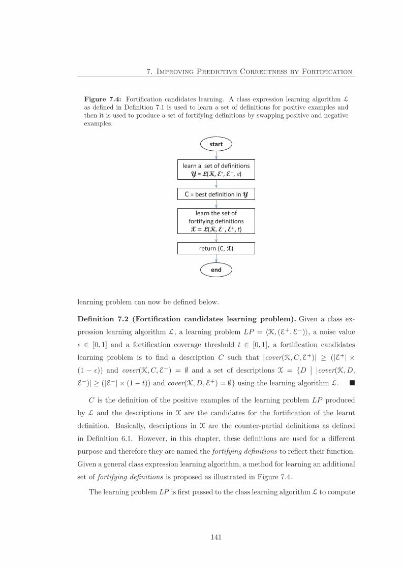
7. Improving Predictive Correctness by Fortification
Figure 7.4: Fortification candidates learning. A class expression learning algorithm L
as defined in Definition 7.1 is used to learn a set of definitions for positive examples andthen it is used to produce a set of fortifying definitions by swapping positive and negativeexamples.
start
learn a set of definitions Y = L(K, E+, E , )
C = best definition in Y
end
learn the set of fortifying definitions X = L(K, E , E+, t)
return (C, X)
learning problem can now be defined below.
Definition 7.2 (Fortification candidates learning problem). Given a class ex-
pression learning algorithm L, a learning problem LP = 〈K, (E+,E−)〉, a noise value
ε ∈ [0, 1] and a fortification coverage threshold t ∈ [0, 1], a fortification candidates
learning problem is to find a description C such that |cover(K, C,E+)| ≥ (|E+| ×(1 − ε)) and cover(K, C,E−) = ∅ and a set of descriptions X = {D ∣∣ |cover(K, D,
E−)| ≥ (|E−| × (1− t)) and cover(K, D,E+) = ∅} using the learning algorithm L. �
C is the definition of the positive examples of the learning problem LP produced
by L and the descriptions in X are the candidates for the fortification of the learnt
definition. Basically, descriptions in X are the counter-partial definitions as defined
in Definition 6.1. However, in this chapter, these definitions are used for a different
purpose and therefore they are named the fortifying definitions to reflect their function.
Given a general class expression learning algorithm, a method for learning an additional
set of fortifying definitions is proposed as illustrated in Figure 7.4.
The learning problem LP is first passed to the class learning algorithm L to compute
141

7. Improving Predictive Correctness by Fortification
the set of definitions of the positive examples. Then, the set of positive and negative
examples are swapped and passed to the algorithm L again together with the fortifica-
tion threshold to compute a set of fortifying definitions. In this step, the fortification
threshold is used as the noise percentage for the swapped learning problem (i.e. the
learning problem with positive and negative examples being swapped). For example, if
the fortification threshold is set to 10%, the learning algorithm can accept descriptions
that cover 10% of the positive examples of the swapped learning problem, i.e. 10% of
the negative examples in the original fortification candidates learning problem. There-
fore, this is a constraint on the selection of the class expression learning algorithm used
for learning the fortification candidates.
A formal fortification candidate learning algorithm is given in Algorithm 7.1. In
this algorithm, a function Accuracy() is used to compute the accuracy of a given
description on the training dataset (see Definition 3.2).
Algorithm 7.1: Fortification candidates learning –FCandLearning(L,K,E+,E−, ε, t).
Input: a class expression leaning algorithm L, a class expression learningproblem 〈K, (E+,E−)〉, a learning noise value ε ∈ [0, 1] (0 means nonoise) and a fortification coverage threshold value t ∈ (0, 1) acts as thelearning noise.
Output: a definition C and a set of fortifying definitions X produced by L suchthat |cover(K, C,E+)| ≥ (|E+| × (1− ε)) and |cover(K, C,E−)| = 0 and∀D ∈ X : |cover(K, D,E−)| ≥ (|E−| × (1− t)) and cover(K, D,E+) = ∅.
1 begin/* perform normal learning to learn the definition for pos.
examples */
2 Y = L(K,E+,E−, ε) /* find a set of definitions using L */
3 select a definition C ∈ Y | ∀E ∈ Y : Accuracy(C) ≥ Accuracy(E)
/* learn the fortifying definitions by reversing the sets of
examples and using the threshold t */
4 X = L(K,E−,E+, t)
5 return (C,X)
The definition of positive examples is called the learnt definition to distinguish with
the fortifying definitions that are the definitions of negative examples.
142
7. Improving Predictive Correctness by Fortification
7.3 Fortification Strategy
In this section, we describe some fortification strategies that aim to select the most
promising candidates for fortification within a set of fortifying definitions produced
by a fortification candidate learning algorithm as described in Algorithm 7.1. The
general idea of our strategies include two steps. The first is to assign each fortifying
definition a score and rank them accordingly to their score. Then, an appropriate
number of fortifying definitions is selected so that it can help to increase the predictive
correctness without decreasing the predictive accuracy.
The strategies address two questions Q2 and Q3 in the problem description section
(Section 7.1): i) how to choose the best candidates for fortification?, and ii) how many
candidates are sufficient for fortification?
7.3.1 Fortification candidates scoring
The aim of fortification candidates scoring is to score the fortifying definitions ac-
cordingly to their potential impact. The scores are then used to rank the fortifying
definitions to support the selection of the most promising fortifying definitions.
A fortifying definition is promising for the fortification if it can help to exclude
the negative examples covered by the learnt concept in the test set (see Figure 7.3b).
However, as the negative examples in the test set are unknown when the learning
takes place, a method for predicting the influence of the fortifying definitions is needed.
Fortifying definitions can be considered as prediction models for the negative examples.
Therefore, scoring the fortifying definitions is basically the estimation of their predictive
power. This motivates two methods for scoring the fortifying definitions. The first is
to consider their training coverage as the factor that represents their predictive power.
The second is to use a dataset, called the (fortification) validation dataset, to evaluate
their predictive power. This dataset does not overlap with the training and test sets.
A fortifying definition that give a good prediction power on the validation dataset is
expected to have a similar performance on the test set.
In addition, the prediction scenario illustrated in Figure 7.3(b) motivates another
method for scoring the fortifying definitions. This method is based on the overlap
143

7. Improving Predictive Correctness by Fortification
between the learnt concept and the fortifying definitions. Here, the concept overlap is
used with the following meaning: Two descriptions are overlapped if they cover some
common instances. The scenario in Figure 7.3(b) shows that if a fortifying definition is
not overlapped with the learnt concept, it will not influence the predictive correctness
even if it covers many negative examples. For example, in Figure 7.3(b), N3 can help
to exclude some negative examples covered by the learnt definition C as it covers
some common negative examples (overlapped) with C. On the other hand, although
N4 covers some negative examples, it does not influence the predictive correctness as
it covers negative examples that are not covered by the learnt definition (i.e. not
overlapped).
Therefore, in this method, the concept similarity measure is used to compute the
overlap between the fortifying definition candidates and the learnt concept. The simi-
larity measure based on both the ABox and TBox of the knowledge base are combined.
The more overlap between a fortifying definition and the learnt concept there is, the
more influence the fortifying definition has in the prediction. The following sections
provide detailed description of our scoring methods.
7.3.1.1 Training coverage scoring
In this method, the training coverage of the fortifying definitions is used as their score.
This information is the result of the training (learning) process and it is associated with
every fortifying definition. The essential idea behind this method is that the training
coverage potentially implies the generality and the predictive power of the fortifying
definitions. The more general a fortifying definition is, the more chance for it to cover
more negative examples in the test set in comparison with a less general definition.
The biggest advantage of this method is that the coverage is available from the
learning process. Therefore, there is no extra computation required for scoring the
fortifying definitions. In addition, high predictive power of the fortifying definitions
(high coverage) may imply a higher chance for it to cover negative examples in the test
set. The score of a fortifying definition C in this method is defined as follows:
score(C) =|cover(K, C,E−)|
|E−| (7.1)
144
7. Improving Predictive Correctness by Fortification
This value is actually the training completeness of the fortifying definition. There-
fore, this information is associated with each fortifying definition and thus it does not
need to be re-computed. In addition, higher priority is given to short fortifying defini-
tions in case the fortifying definitions have the same coverage on E−. In the top-down
approach, shorter definitions are usually more general than longer ones. Therefore, this
factor is used as a tiebreaker in scoring the fortifying definitions. It can now be defined
as below.
Definition 7.3 (Training coverage score). Let LP = 〈K, (E+,E−)〉 be a learning
problem, C a fortifying definition learnt from LP, max fdlength the maximal length of
all fortifying definitions learnt and length(C ) a function that returns the length of the
definition C. The score of the fortifying definition C based on the training coverage
scoring method is defined as follows:
TCScore(C) =|cover(K, C,E−)| ×max fdlength− length(C)
|E−| ×max fdlength(7.2)
�
The multiplication cover(K, C,E−) with max fdlength in Equation (7.2) is to en-
sure the training coverage is used as the primary criteria when ranking (sorting) the
fortifying definition and the division is to scale the score into [0, 1]. The algorithm for
scoring a set of fortifying definitions is given in Algorithm 7.2.
7.3.1.2 Fortification concept similarity scoring
In this strategy, the overlap between the fortifying and the learnt definitions is used to
score the fortifying definitions.
Concept overlap measure
There are several approaches to assess the overlap between concepts that are based on
the computation of similarity between concepts. The first approach is based on the
overlap between instances in the ABox of the knowledge base [33, 34, 44, 68]. There
are also some other approaches that use the refinement or subtraction operators in
description logics such as [120, 130]. In our method, the overlap between concepts is
145
7. Improving Predictive Correctness by Fortification
Algorithm 7.2: Training coverage scoring – TCScore(X,K,E+,E−).Input: a set of fortifying definitions X and a learning problem
LP = 〈K, (E+,E−)〉Output: a set of scored fortifying definitions based on Equation (7.2).
1 begin2 max length = 0 /* maximal length of the fortifying definitions */
3 Y = ∅ /* set of scored fortifying definitions */
/* calculate the maximal length of the fortifying definitions */
4 foreach C ∈ X do5 if max length < length(C) then max length = length(C )
/* compute the score for the fortifying definitions */
6 foreach C ∈ X do7 coverC = cover(K, C,E−) /* set of neg.examples covered by C */
8 scoreC = (coverC ×max length− length(C)) / (|E+| ×max length)9 Y = Y ∪ {(C, scoreC)}
10 return Y
computed based on the instances in the ABox. Basically, overlap between concepts is
measured by the ratio between common instances over total instances covered by both
descriptions (i.e. the Jaccard coefficient) as follows:
JOverlap(C,D) =|cover(K, C,E) ∩ cover(K, D,E)||cover(K, C,E) ∪ cover(K, D,E)| (7.3)
where C,D are two descriptions, E is a set of instances in which the similarity is tested
and K is the knowledge based that contains the concepts and instances.
In our method, the similarity measure proposed in [34] is adopted, which extends
Equation (7.3) with the reduction by the major incidence of the intersection with
respect to either concept (see [34] for more details).
overlap(C,D) =|cover(K, C,E) ∩ cover(K, D,E)||cover(K, C,E) ∪ cover(K, D,E)| ×
max
( |cover(K, C,E) ∩ cover(K, D,E)||cover(K, C,E)| ,
|cover(K, C,E) ∩ cover(K, D,E)||cover(K, D,E)|
)(7.4)
146

7. Improving Predictive Correctness by Fortification
The following example illustrates the overlap calculation between concepts defined
in Equation (7.4).
Example 7.1 (Concept similarity calculation). Let NC be a set of concept names,
NR be a set of role names, K = (T,A) be a knowledge base with TBox T and ABox A,
and E be a set of instances of the concepts in K as follows:
• NC = {Person,Male,Female,Mother,Father,Child}
• NR = {married, hasChild, hasParent}
• T =
⎧⎪⎪⎪⎪⎪⎨⎪⎪⎪⎪⎪⎩
Male Person,Female Person,Male ≡ ¬Female
Mother ≡ Female � ∃hasChild.PersonFather ≡ Male � ∃hasChild.PersonChild ≡ Person � ∃hasParent.Person
⎫⎪⎪⎪⎪⎪⎬⎪⎪⎪⎪⎪⎭
• A =
⎧⎪⎪⎪⎪⎪⎪⎪⎪⎪⎪⎪⎪⎪⎪⎨⎪⎪⎪⎪⎪⎪⎪⎪⎪⎪⎪⎪⎪⎪⎩
Person(a),Female(a), hasChild(a, b), hasChild(a, c)
Person(b),Male(b), hacChild(b, d), hasParent(b, a)
Person(c),Male(c), hasChild(c, e), hasParent(c, a)
Person(e),Female(e), hacParent(e, c)
Person(d),Female(d), hasChild(d, h), hasParent(d, b),marriedTo(d, g)
Person(h),Female(h), hasParent(h, d), hasParent(h, g)
Person(g),Male(g),marriedTo(g, d))
⎫⎪⎪⎪⎪⎪⎪⎪⎪⎪⎪⎪⎪⎪⎪⎬⎪⎪⎪⎪⎪⎪⎪⎪⎪⎪⎪⎪⎪⎪⎭
• E = {a, b, c, d, e, g, h}
Then, examples of the computation of the overlap between concepts are given below.
(1) overlap(Person, Female) :
� cover(K,Person,E) = {a, b, c, d, e, g, h}� cover(K,Female,E) = {a, d, e, h}⇒ overlap(Person,Female) =
|{a, d, e, h}||{a, b, c, d, e, g, h}|×
max
( |{a, d, e, h}||{a, b, c, d, e, g, h}| ,
|{a, d, e, h}||{a, d, e, h}|
)
=4
7= 0.571
147
7. Improving Predictive Correctness by Fortification
(2) overlap(Female,Mother) :
� cover(K,Parent,E) = {a, b, c, d, g}� cover(K,Female,E) = {a, d, e, h}⇒ overlap(Female, Mother) =
|{a, d}||{a, b, c, d, e, g, h}|×
max
( |{a, d}||{a, b, c, d, g}| ,
|{a, d}||{a, d, e, h}|
)
=2
7× 2
4=
1
7= 0.143
(3) overlap(C, D) : where,
C ≡ Person � ∃hasChild.PersonD ≡ Person � ∃marriedTo.Person
� cover(K, C,E) = {a, b, c, d, g}� cover(K, D,E) = {d, g}⇒ overlap(C, D) =
|{d, g}||{a, b, c, d, g}| ×max
( |{d, g}||{a, b, c, d, g}| ,
|{d, g}||{d, g}|
)
=2
5= 0.4
�
The algorithm for measuring the overlap between two concepts is given in Alg. 7.3.
Concept similarity measure
The method above computes the overlap between two concepts based on the ABox,
i.e. the instances (or the snapshot) of the knowledge base. As the result, it is sen-
sitive to the change of instances of the knowledge base. Therefore, in our fortifying
definition scoring is based on the overlap between the learnt concept and the fortify-
ing definition, the semantics of the concepts in the descriptions is used to strengthen
the measure of Equation (7.4) to reduce the dependency of the measure on the ABox.
This method uses the semantics of the concepts defined by the TBox (e.g. subclass,
sub-role, equivalent class, etc.) to estimate the similarity between concepts. Here, the
word similarity is used to imply the independence of the measure on the instances or
148

7. Improving Predictive Correctness by Fortification
Algorithm 7.3: Concept overlap measure – COverlap(C, D, K,E)
Input: Two description C, D, a knowledge base K = (T,A) and a set ofinstances E.
Output: an overlap value between C and D as defined in Equation (7.4).1 begin
/* see Definition 3.1 for definition of function cover () */
2 intersection = cover(K, C,E) ∩ cover(K, D,E)3 union = cover(K, C,E) ∪ cover(K, D,E)
/* overlap without dissimilarity factor */
4 basicOverlap = |intersection| / |union| /* |X|: no.of X’s elements */
/* dissimilarity factor */
5 dissimilarity =max(|intersection| / |cover(K, C,E)|, |intersection| / |cover(K, D,E)|)
6 return (basicOverlap× dissimilarity)
snapshot of the knowledge base and the stability by using the semantics of the concepts
in the TBox. Intuitively, concept similarity is more general than concept overlap. The
overlap between concepts indicates the similarity between them. However, two similar
descriptions do not necessarily have common instances. Similarity implies the potential
or probability of the overlap between descriptions. The more similar the concepts are,
the more they are likely to have common instances.
There is no widely accepted method for measuring the similarity between descrip-
tions using the TBox. As the above overlap computation uses a particular ABox, the
amount of the overlap can always be computed. On the other hand, concepts them-
selves sometimes do not provide sufficient information for estimation of their similarity.
For example, given a concept hierarchy as shown in Figure 7.5, there may not have any
information about the similarity between the concepts Father and Brother without a
particular ABox. A father may be a brother or not, depending upon the particular
circumstances.
However, in some cases, semantics of the concepts may help to estimate the chance
of being similar between concepts or compare the chance of being similar amongst con-
cepts. For example, the similarity between Child and Son is higher than the similarity
between Brother and Father. In addition, if a statistical distribution is identified for
the distribution of the instances of Child, Son and Daughter concepts, we can estimate
149

7. Improving Predictive Correctness by Fortification
Figure 7.5: Family concepts hierarchy. Arrows represent subclass relations (superclass−→ subclass)
Thing
Person
Male Female Parent Child
Brother Father Son Mother Daughter Sister Dad Mom
a specific value for the similarity between Child and Son or Child and Daughter. For
example, if the instances of these three concepts follow the uniform distribution [73],
the probability of an instance of the concept Child being also an instance of the concept
Son is about 50%. This probability can be used to estimate the similarity between the
above concepts.
In this method, the Jaccard coefficient similarity and the semantics of the concepts
defined in the TBox are used to estimate the similarity between two descriptions based
on their composite atomic concepts and roles. Jaccard is a popular method to compute
the overlap between (elements of) two sets [67, 110]. It is defined as the ratio between
the intersection of the two sets over the union of the two sets. Given two descriptions
C and D in disjunctive normal form: C ≡ C1 � . . . � Cn and D ≡ D1 � . . . �Dm, then
we define the Jaccard similarity between C and D is the maximal similarity of all pair
of disjuncts (Ci, Dj) as follows:
JSim�(C,D) =
⎧⎪⎪⎨⎪⎪⎩
1, if C ≡ D
0, if C �D ≡ ⊥maxi=1..n,j=1..m JSim(Ci, Dj)
(7.5)
where JSim(Ci, Dj) is the Jaccard similarity between two descriptions with no disjunc-
tion. The max function used in the case of disjunction is one of the possible methods
that is chosen due to its simplicity. In addition, the intuition behind this selection is
that sub-concepts in disjunctions account for a certain aspect of the overall concept.
Hence, if they perfectly match on one aspect, then their individuals may be interchange-
150
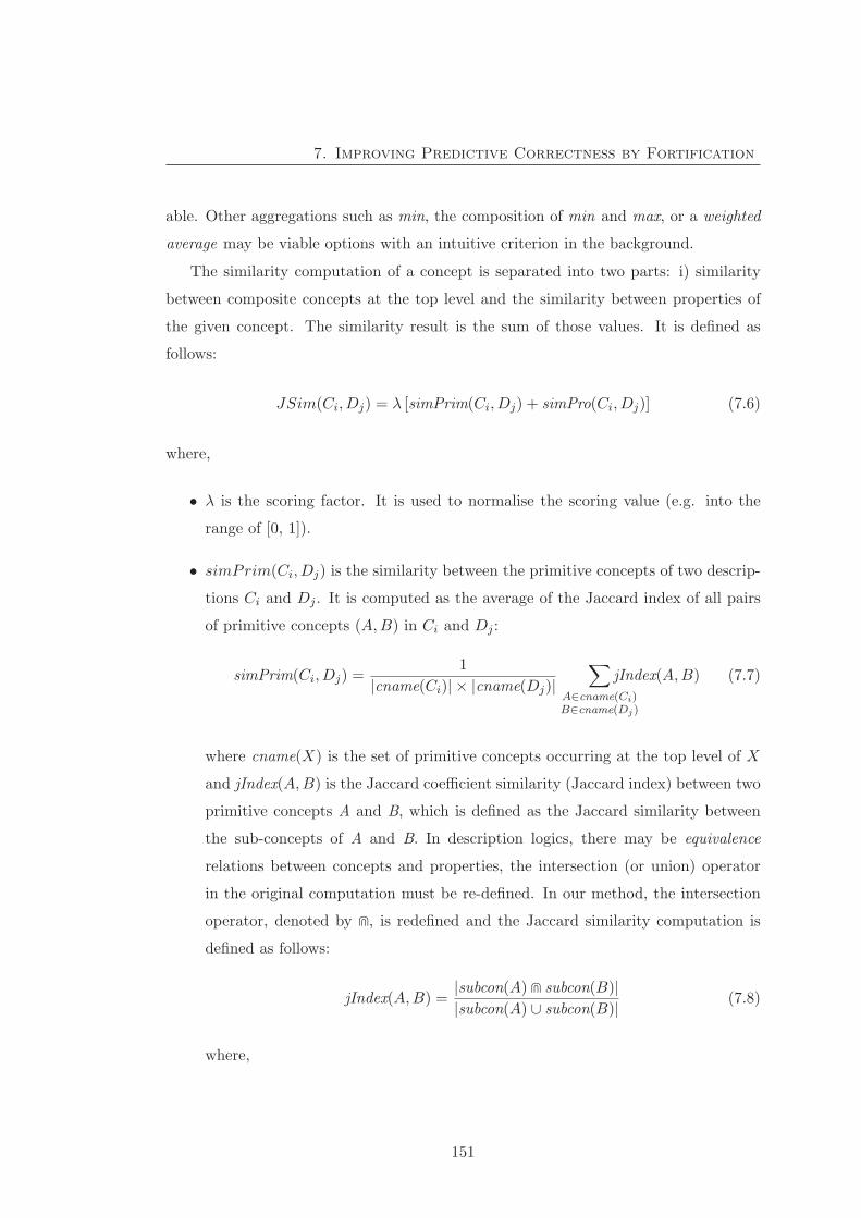
7. Improving Predictive Correctness by Fortification
able. Other aggregations such as min, the composition of min and max, or a weighted
average may be viable options with an intuitive criterion in the background.
The similarity computation of a concept is separated into two parts: i) similarity
between composite concepts at the top level and the similarity between properties of
the given concept. The similarity result is the sum of those values. It is defined as
follows:
JSim(Ci, Dj) = λ [simPrim(Ci, Dj) + simPro(Ci, Dj)] (7.6)
where,
• λ is the scoring factor. It is used to normalise the scoring value (e.g. into the
range of [0, 1]).
• simPrim(Ci, Dj) is the similarity between the primitive concepts of two descrip-
tions Ci and Dj . It is computed as the average of the Jaccard index of all pairs
of primitive concepts (A,B) in Ci and Dj :
simPrim(Ci, Dj) =1
|cname(Ci)| × |cname(Dj)|∑
A∈cname(Ci)B∈cname(Dj)
jIndex(A,B) (7.7)
where cname(X) is the set of primitive concepts occurring at the top level of X
and jIndex(A,B) is the Jaccard coefficient similarity (Jaccard index) between two
primitive concepts A and B, which is defined as the Jaccard similarity between
the sub-concepts of A and B. In description logics, there may be equivalence
relations between concepts and properties, the intersection (or union) operator
in the original computation must be re-defined. In our method, the intersection
operator, denoted by �, is redefined and the Jaccard similarity computation is
defined as follows:
jIndex(A,B) =|subcon(A) � subcon(B)||subcon(A) ∪ subcon(B)| (7.8)
where,
151
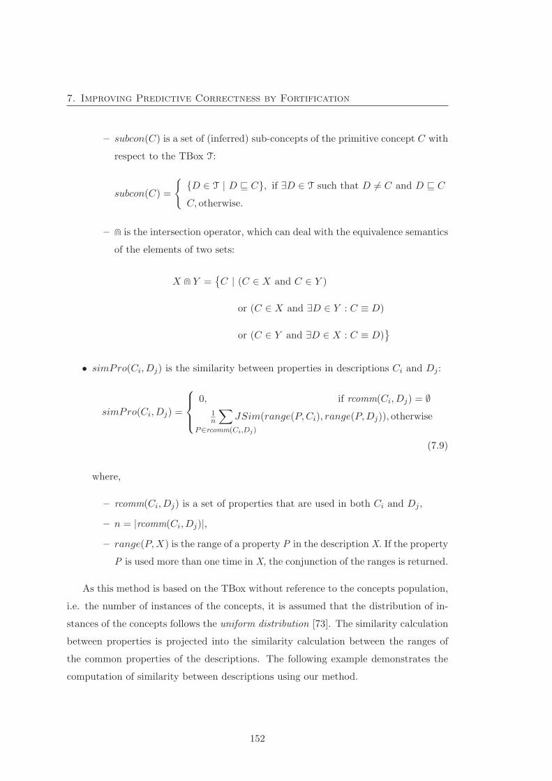
7. Improving Predictive Correctness by Fortification
– subcon(C) is a set of (inferred) sub-concepts of the primitive concept C with
respect to the TBox T:
subcon(C) =
{{D ∈ T | D C}, if ∃D ∈ T such that D �= C and D C
C, otherwise.
– � is the intersection operator, which can deal with the equivalence semantics
of the elements of two sets:
X � Y ={C | (C ∈ X and C ∈ Y )
or (C ∈ X and ∃D ∈ Y : C ≡ D)
or (C ∈ Y and ∃D ∈ X : C ≡ D)}
• simPro(Ci, Dj) is the similarity between properties in descriptions Ci and Dj :
simPro(Ci, Dj) =
⎧⎪⎨⎪⎩
0, if rcomm(Ci, Dj) = ∅1n
∑P∈rcomm(Ci,Dj)
JSim(range(P,Ci), range(P,Dj)), otherwise
(7.9)
where,
– rcomm(Ci, Dj) is a set of properties that are used in both Ci and Dj ,
– n = |rcomm(Ci, Dj)|,– range(P,X) is the range of a property P in the description X. If the property
P is used more than one time in X, the conjunction of the ranges is returned.
As this method is based on the TBox without reference to the concepts population,
i.e. the number of instances of the concepts, it is assumed that the distribution of in-
stances of the concepts follows the uniform distribution [73]. The similarity calculation
between properties is projected into the similarity calculation between the ranges of
the common properties of the descriptions. The following example demonstrates the
computation of similarity between descriptions using our method.
152

7. Improving Predictive Correctness by Fortification
Example 7.2 (Description similarity calculation using Jaccard method). This
example demonstrates the computation of similarity between concepts in disjunctive
normal form described in Equation (7.6). To scale the similarity value into [0, 1],
λ = 1/2 is chosen if there are both concepts and properties in the descriptions and
λ = 1 otherwise. Given a TBox as shown in Figure 7.5, similarity of some concepts
based on Jaccard method are computed as follows:
(1) JSim(Male, Female): as these descriptions have no property, the similarity be-
tween concepts (the first part of Equation (7.6)) is computed as follows:
� simPrim(Male,Famale) = jIndex(Male,Female)
=|subcon(Male) � subcon(Female)||subcon(Male) ∪ subcon(Female)|
=|{Dad,Father, Son,Brother} � {Mom,Mother,Daughter, Sister}||{Dad,Father, Son,Brother} ∪ {Mom,Mother,Daughter, Sister}| = 0
⇒ JSim(Male, Female) = 0
(2) JSim(Female, Mother) : similar to the above example, we have:
� simPrim(Female, Mother) = jIndex(Female, Mother)
=|subcon(Female) � subcon(Mother)||subcon(Female) ∪ subcon(Mother)|
=|{Mom, Mother, Daughter, Sister} � {Mother}||{Mom, Mother, Daughter, Sister} ∪ {Mother}| =
2
4= 0.5
⇒ JSim(Female, Mother) = 0.5
(3) JSim(C,D), where:
C ≡ Person � ∃hasChild.PersonD ≡ Person � ∃marriedTo.Person
We have:
� simPrim(C,D) = jIndex(C,D)
=|subcon(Person) � subcon(Person)||subcon(Person) ∪ subcon(Person)| = 1
153
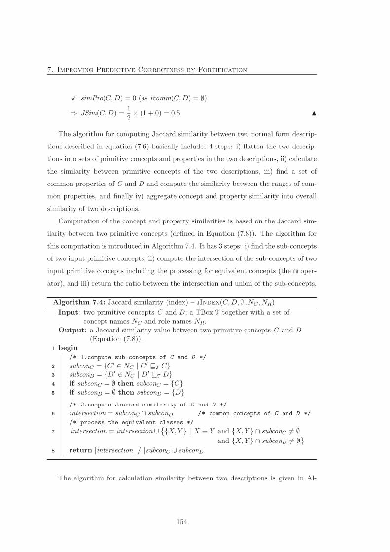
7. Improving Predictive Correctness by Fortification
� simPro(C,D) = 0 (as rcomm(C,D) = ∅)⇒ JSim(C,D) =
1
2× (1 + 0) = 0.5 �
The algorithm for computing Jaccard similarity between two normal form descrip-
tions described in equation (7.6) basically includes 4 steps: i) flatten the two descrip-
tions into sets of primitive concepts and properties in the two descriptions, ii) calculate
the similarity between primitive concepts of the two descriptions, iii) find a set of
common properties of C and D and compute the similarity between the ranges of com-
mon properties, and finally iv) aggregate concept and property similarity into overall
similarity of two descriptions.
Computation of the concept and property similarities is based on the Jaccard sim-
ilarity between two primitive concepts (defined in Equation (7.8)). The algorithm for
this computation is introduced in Algorithm 7.4. It has 3 steps: i) find the sub-concepts
of two input primitive concepts, ii) compute the intersection of the sub-concepts of two
input primitive concepts including the processing for equivalent concepts (the � oper-
ator), and iii) return the ratio between the intersection and union of the sub-concepts.
Algorithm 7.4: Jaccard similarity (index) – jIndex(C,D,T, NC , NR)
Input: two primitive concepts C and D ; a TBox T together with a set ofconcept names NC and role names NR.
Output: a Jaccard similarity value between two primitive concepts C and D(Equation (7.8)).
1 begin/* 1.compute sub-concepts of C and D */
2 subconC = {C ′ ∈ NC | C ′ T C}3 subconD = {D′ ∈ NC | D′ T D}4 if subconC = ∅ then subconC = {C}5 if subconD = ∅ then subconD = {D}
/* 2.compute Jaccard similarity of C and D */
6 intersection = subconC ∩ subconD /* common concepts of C and D */
/* process the equivalent classes */
7 intersection = intersection ∪ {{X,Y } | X ≡ Y and {X,Y } ∩ subconC �= ∅and {X,Y } ∩ subconD �= ∅}
8 return |intersection| / |subconC ∪ subconD|
The algorithm for calculation similarity between two descriptions is given in Al-
154

7. Improving Predictive Correctness by Fortification
gorithm 7.5. Firstly, the similarity between primitive concepts is computed based on
the Jaccard coefficient calculation implemented in Algorithm 7.4. Then, the similarity
for the properties of the descriptions is calculated by recursively calling the similarity
calculation for the ranges of the common properties of the two descriptions. The simi-
larity between two description is the sum of concept similarity and property similarity
multiply with the scoring factor λ.
Fortifying definition scoring
The score of the fortifying definitions based on the concept overlap and similarity is
computed as follows:
Definition 7.4 (Concept similarity score). Let C be a fortifying definition, D a
learnt definition from the same learning problem, overlap(C, D) a function function that
measures the overlap between C and D as defined in Equation (7.4) and JSim�(C,D)
a function that compute the similarity between C and D as defined in Equation (7.5).
The score of C is defined as follows:
CSScore(C) = overlap(C,D) + JSim�(C,D) �
The overlap (based on ABox) and similarity (based on TBox) in Definition 7.4 seem
to be treated equally. However, we can adjust the impact of these parts according to
the particular learning problem using the similarity scoring factor in Definition 7.6.
The following example illustrates the calculation of similarity between descriptions
using the fortification concepts similarity scoring method.
Example 7.3. Given a knowledge base as shown in Example 7.1, then the calculation
of fortifying definition score is given below.
(1) CSScore(Female,Mother):
� overlap(Female, Mother) = 0.286 (see Example 7.1).
� JSim � (Female, Mother) = 0.5 (see Example 7.2).
⇒ CSScore(Female, Mother) = (0.286 + 0.5) = 0.786
155

7. Improving Predictive Correctness by Fortification
Algorithm 7.5: Jaccard similarity scoring – JSim(C,D, λ,T, NC , NR)
Input: two descriptions in normal form C, D ; the scoring weighting factor λ; aTBox T together with a set of concept names NC and role names NR.
Output: Jaccard similarity value between C and D (Equation (7.6)).1 begin
/* 1.compute similarity between primitive concepts */
/* 1.1.get lists of primitive concepts occurring at the 1st level of C
and D */
2 primC = {C ′ | C ′ ∈ NC and C ′ occurs at 1st level of C}3 primD = {D′ | D′ ∈ NC and D′ occurs at 1st level of D}
/* 1.2.similarity of all pairs of disjuncts primitive concepts */
4 csim = 0 /* primitive concepts similarity */
5 foreach X ∈ primC do6 foreach Y ∈ primD do7 csim += jIndex(X,Y,T, NC , NR)
8 csim = csim / (|primC |.|primD|) /* calculate the avg.value */
/* 2.calculate similarity between common properties of C and D */
/* 2.1.find list of common properties between C and D */
9 proC = {C ′ | C ′ ∈ NR and C ′ occurs at the 1st level of C}10 proD = {D′ | D′ ∈ NR and D′ occurs at the 1st level of D}11 pcomm = proC ∩ proD /* common properties of C and D */
/* 2.2.compute the similarity of the common properties */
12 psim = 0 /* properties similarity */
13 if |pcomm| > 0 then14 foreach P ∈ pcomm do15 rangePC = {�C ′ | ∃P.C ′ or ∀P.C ′ occurs in C}16 rangePD = {�D′ | ∃P.D′ or ∀P.D′ occurs in D}17 psim += JSim(rangePC , rangePD, λ,T, NC , NR)
18 psim = psim / |pcomm|19 return λ× (csim+ psim)
156
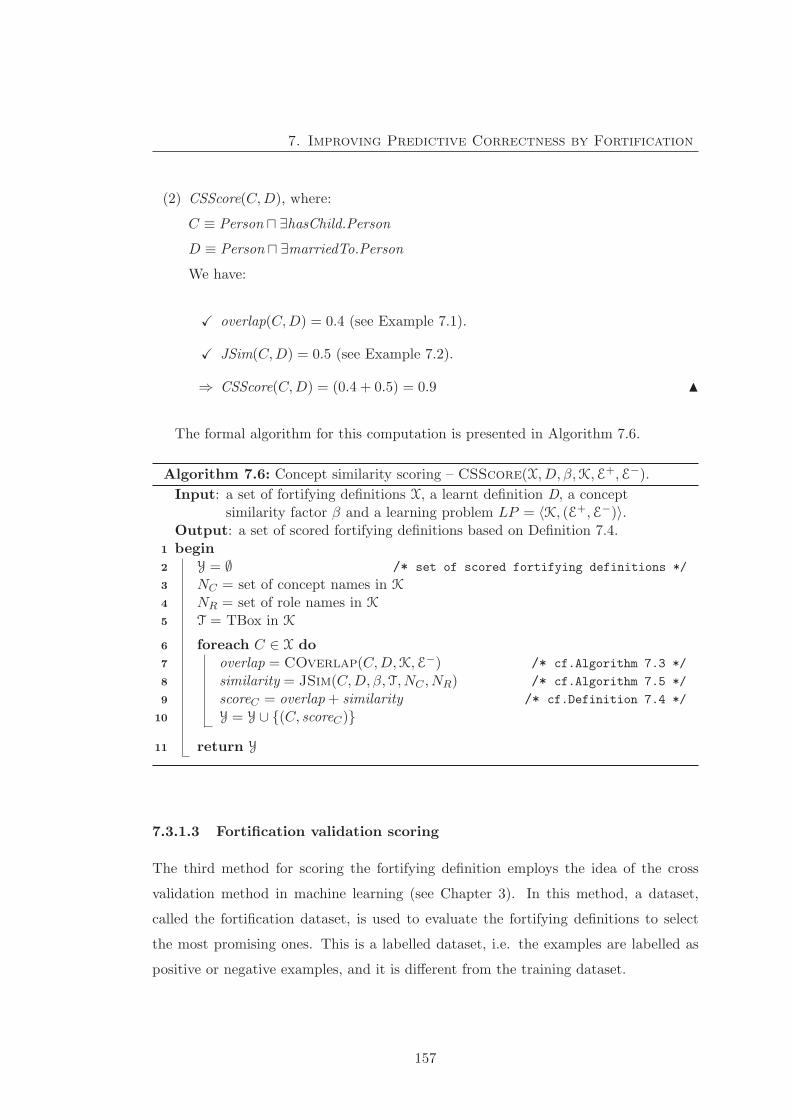
7. Improving Predictive Correctness by Fortification
(2) CSScore(C,D), where:
C ≡ Person � ∃hasChild.PersonD ≡ Person � ∃marriedTo.Person
We have:
� overlap(C,D) = 0.4 (see Example 7.1).
� JSim(C,D) = 0.5 (see Example 7.2).
⇒ CSScore(C,D) = (0.4 + 0.5) = 0.9 �
The formal algorithm for this computation is presented in Algorithm 7.6.
Algorithm 7.6: Concept similarity scoring – CSScore(X, D, β,K,E+,E−).Input: a set of fortifying definitions X, a learnt definition D, a concept
similarity factor β and a learning problem LP = 〈K, (E+,E−)〉.Output: a set of scored fortifying definitions based on Definition 7.4.
1 begin2 Y = ∅ /* set of scored fortifying definitions */
3 NC = set of concept names in K
4 NR = set of role names in K
5 T = TBox in K
6 foreach C ∈ X do7 overlap = COverlap(C,D,K,E−) /* cf.Algorithm 7.3 */
8 similarity = JSim(C,D, β,T, NC , NR) /* cf.Algorithm 7.5 */
9 scoreC = overlap+ similarity /* cf.Definition 7.4 */
10 Y = Y ∪ {(C, scoreC)}11 return Y
7.3.1.3 Fortification validation scoring
The third method for scoring the fortifying definition employs the idea of the cross
validation method in machine learning (see Chapter 3). In this method, a dataset,
called the fortification dataset, is used to evaluate the fortifying definitions to select
the most promising ones. This is a labelled dataset, i.e. the examples are labelled as
positive or negative examples, and it is different from the training dataset.
157
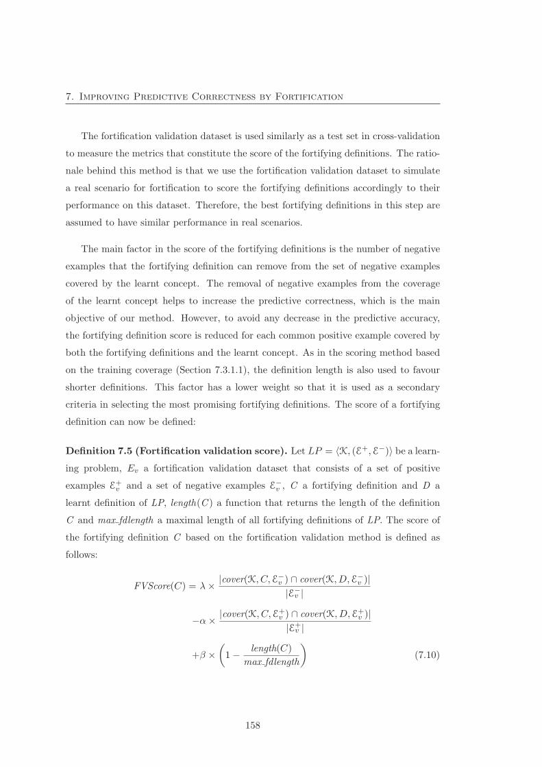
7. Improving Predictive Correctness by Fortification
The fortification validation dataset is used similarly as a test set in cross-validation
to measure the metrics that constitute the score of the fortifying definitions. The ratio-
nale behind this method is that we use the fortification validation dataset to simulate
a real scenario for fortification to score the fortifying definitions accordingly to their
performance on this dataset. Therefore, the best fortifying definitions in this step are
assumed to have similar performance in real scenarios.
The main factor in the score of the fortifying definitions is the number of negative
examples that the fortifying definition can remove from the set of negative examples
covered by the learnt concept. The removal of negative examples from the coverage
of the learnt concept helps to increase the predictive correctness, which is the main
objective of our method. However, to avoid any decrease in the predictive accuracy,
the fortifying definition score is reduced for each common positive example covered by
both the fortifying definitions and the learnt concept. As in the scoring method based
on the training coverage (Section 7.3.1.1), the definition length is also used to favour
shorter definitions. This factor has a lower weight so that it is used as a secondary
criteria in selecting the most promising fortifying definitions. The score of a fortifying
definition can now be defined:
Definition 7.5 (Fortification validation score). Let LP = 〈K, (E+,E−)〉 be a learn-ing problem, Ev a fortification validation dataset that consists of a set of positive
examples E+v and a set of negative examples E−
v , C a fortifying definition and D a
learnt definition of LP, length(C ) a function that returns the length of the definition
C and max fdlength a maximal length of all fortifying definitions of LP. The score of
the fortifying definition C based on the fortification validation method is defined as
follows:
FVScore(C) = λ× |cover(K, C,E−v ) ∩ cover(K, D,E−
v )||E−
v |
−α× |cover(K, C,E+v ) ∩ cover(K, D,E+
v )||E+
v |
+β ×(1− length(C)
max fdlength
)(7.10)
158
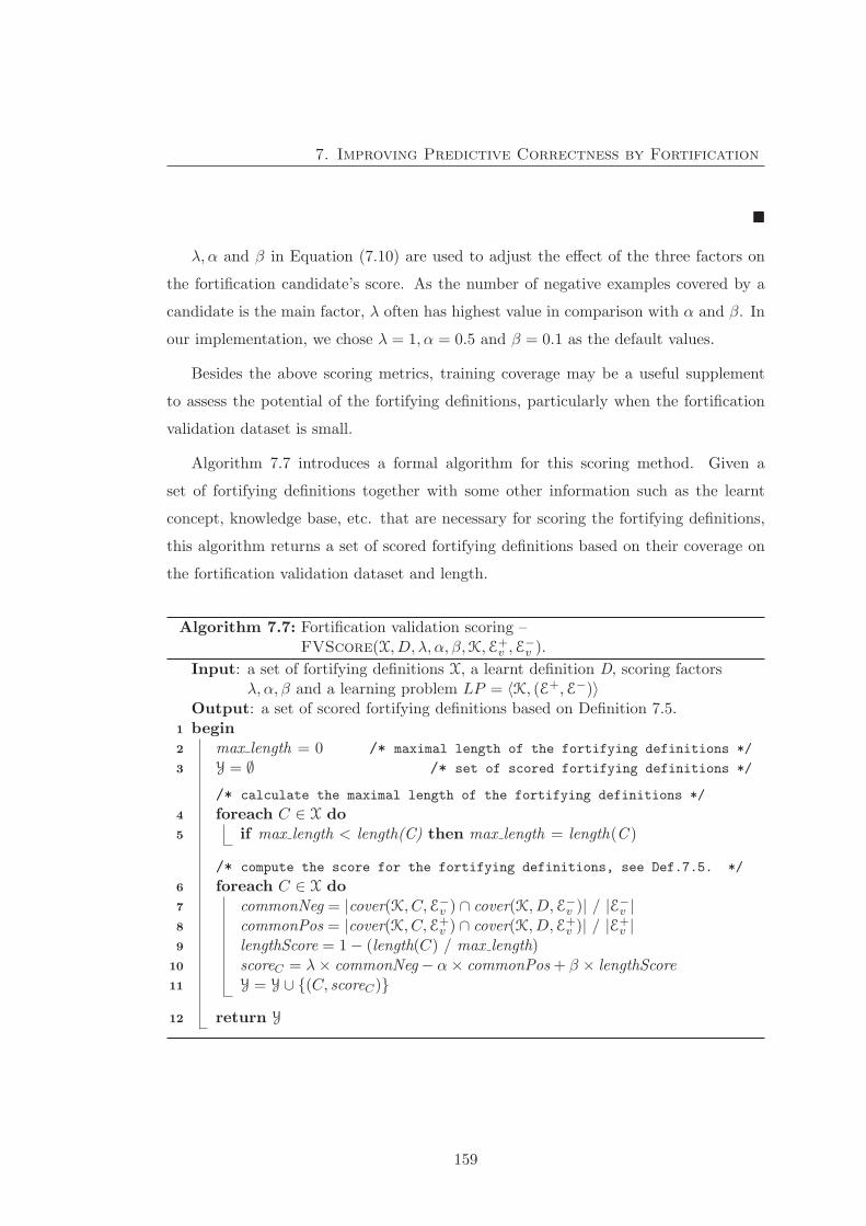
7. Improving Predictive Correctness by Fortification
�
λ, α and β in Equation (7.10) are used to adjust the effect of the three factors on
the fortification candidate’s score. As the number of negative examples covered by a
candidate is the main factor, λ often has highest value in comparison with α and β. In
our implementation, we chose λ = 1, α = 0.5 and β = 0.1 as the default values.
Besides the above scoring metrics, training coverage may be a useful supplement
to assess the potential of the fortifying definitions, particularly when the fortification
validation dataset is small.
Algorithm 7.7 introduces a formal algorithm for this scoring method. Given a
set of fortifying definitions together with some other information such as the learnt
concept, knowledge base, etc. that are necessary for scoring the fortifying definitions,
this algorithm returns a set of scored fortifying definitions based on their coverage on
the fortification validation dataset and length.
Algorithm 7.7: Fortification validation scoring –FVScore(X, D, λ, α, β,K,E+
v ,E−v ).
Input: a set of fortifying definitions X, a learnt definition D, scoring factorsλ, α, β and a learning problem LP = 〈K, (E+,E−)〉
Output: a set of scored fortifying definitions based on Definition 7.5.1 begin2 max length = 0 /* maximal length of the fortifying definitions */
3 Y = ∅ /* set of scored fortifying definitions */
/* calculate the maximal length of the fortifying definitions */
4 foreach C ∈ X do5 if max length < length(C) then max length = length(C )
/* compute the score for the fortifying definitions, see Def.7.5. */
6 foreach C ∈ X do7 commonNeg = |cover(K, C,E−
v ) ∩ cover(K, D,E−v )| / |E−
v |8 commonPos = |cover(K, C,E+
v ) ∩ cover(K, D,E+v )| / |E+
v |9 lengthScore = 1− (length(C) / max length)
10 scoreC = λ× commonNeg− α× commonPos+ β × lengthScore11 Y = Y ∪ {(C, scoreC)}12 return Y
159
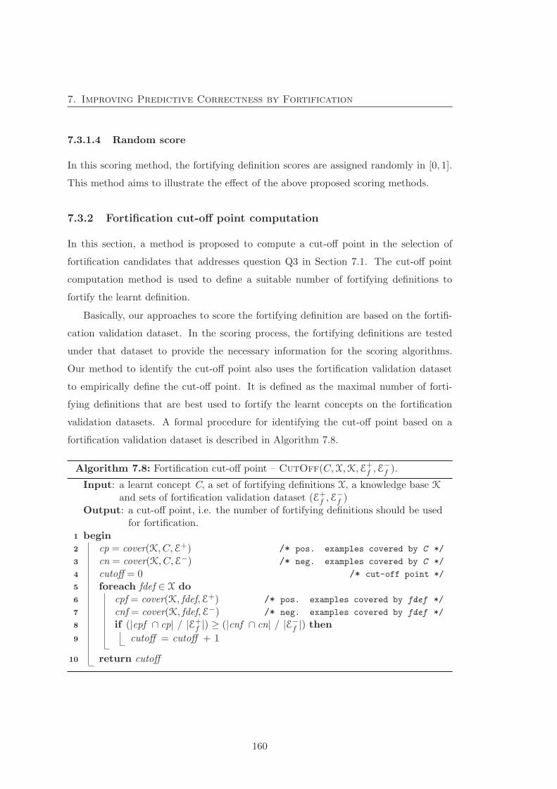
7. Improving Predictive Correctness by Fortification
7.3.1.4 Random score
In this scoring method, the fortifying definition scores are assigned randomly in [0, 1].
This method aims to illustrate the effect of the above proposed scoring methods.
7.3.2 Fortification cut-off point computation
In this section, a method is proposed to compute a cut-off point in the selection of
fortification candidates that addresses question Q3 in Section 7.1. The cut-off point
computation method is used to define a suitable number of fortifying definitions to
fortify the learnt definition.
Basically, our approaches to score the fortifying definition are based on the fortifi-
cation validation dataset. In the scoring process, the fortifying definitions are tested
under that dataset to provide the necessary information for the scoring algorithms.
Our method to identify the cut-off point also uses the fortification validation dataset
to empirically define the cut-off point. It is defined as the maximal number of forti-
fying definitions that are best used to fortify the learnt concepts on the fortification
validation datasets. A formal procedure for identifying the cut-off point based on a
fortification validation dataset is described in Algorithm 7.8.
Algorithm 7.8: Fortification cut-off point – CutOff(C,X,K,E+f ,E
−f ).
Input: a learnt concept C, a set of fortifying definitions X, a knowledge base K
and sets of fortification validation dataset (E+f ,E
−f )
Output: a cut-off point, i.e. the number of fortifying definitions should be usedfor fortification.
1 begin2 cp = cover(K, C,E+) /* pos. examples covered by C */
3 cn = cover(K, C,E−) /* neg. examples covered by C */
4 cutoff = 0 /* cut-off point */
5 foreach fdef ∈ X do6 cpf = cover(K, fdef,E+) /* pos. examples covered by fdef */
7 cnf = cover(K, fdef,E−) /* neg. examples covered by fdef */
8 if (|cpf ∩ cp| / |E+f |) ≥ (|cnf ∩ cn| / |E−
f |) then9 cutoff = cutoff + 1
10 return cutoff
160

7. Improving Predictive Correctness by Fortification
7.4 Evaluation
Efficacy of fortification was evaluated by implementing our methods in CELOE, Par-
CEL and SPaCEL and conducting several experiments using these algorithms. These
algorithms use different approaches in class expression logic learning and thus this se-
lection allows a thorough assessment of the fortification approach. The fortification
candidates generation algorithm (Algorithm 7.1) was first implemented in CELOE and
ParCEL. For SPaCEL, its unused counter-partial definitions were employed as the for-
tifying definitions. Then, an evaluation methodology was designed based on the eval-
uation methodology described in Chapter 3 and the fortification strategies in Section
7.3 to measure the metrics with and without the fortification.
7.4.1 Fortification evaluation methodology
To evaluate the fortification approach, we used 10-fold cross-validation on the learning
problems introduced in Chapter 3. In the evaluation of fortification, in addition to the
training and test sets, another dataset, called the fortification validation dataset, was
also needed to suppose the fortification strategies (see Sections 7.3.1.2 and 7.3.1.3).
Therefore, in each fold, we used 8 parts for training, 1 for fortification validation and
1 for testing.
In addition, the procedure for measuring the evaluation metrics was also revised to
involve the fortification. Each fold of the cross-validation includes the following tasks:
1. Learn the concept C and a set of fortifying definitions X using the training set of
the validation dataset i.
2. Score the fortifying definitions in X using a fortification strategy and sort them
according to their score. The fortification validation set in validation dataset i is
used if it is needed by the fortification strategy.
3. Compute the cut-off point for the fortification.
4. Measure the evaluation metrics (accuracy, completeness and correctness) for the
learnt definition C using the test set in evaluation dataset i.
161
7. Improving Predictive Correctness by Fortification
5. Perform the fortification by making the conjunction: C = C � ¬⊔Di, ∀Di ∈ X
such that Di is within the cut-off point.
6. Recompute the evaluation metrics for the fortified definition C.
7.4.2 Experimental results
This section provides the experimental results of the fortification approach on CELOE,
ParCEL and SPaCEL. In this evaluation, the predictive accuracy, correctness and com-
pleteness with and without fortification of each algorithm will be compared. In this
approach, a trade-off between the predictive correctness and completeness is expected.
Therefore, the baseline used to assess the success of this approach is that the average
predictive correctness with fortification is higher than for the original algorithm and
the average predictive accuracy of the fortification is not lower than for the original
algorithm. However, the assessment of the achievement should also take the predictive
accuracy without fortification into consideration. For learning problems where learn-
ing algorithm achieved 100% predictive correctness, keeping the predictive accuracy
unchanged is considered to be a good achievement.
The following subsections will provide the experimental results for the three learn-
ing algorithms. The four fortification scoring strategies training coverage, concept
similarity, fortification validation, and randomly scoring are named TCScore, CSScore,
FVScore and Random respectively. The experimental results without fortification are
also presented and compared with the fortification results. As described in Section
7.4.1, the training sets of the learning problems in these experiments is smaller than
the training sets used in the experiments in Chapters 5 and 6. Therefore, the experi-
mental results without fortification in this section may be different from the results in
the previous experiment. The experimental results with full training set in the previous
experiments are also included for reference (called “Full training”).
The t-test at the 95% confidence level was conducted to check the statistical signif-
icant differences between the experimental results with and without fortification.
162
7. Improving Predictive Correctness by Fortification
Experimental results on CELOE
Table 7.1 shows the experimental result of fortification on the CELOE algorithm. For
the low and medium complexity learning problems (Group 1 in the result table),
CELOE achieved 100% of accuracy for most of them (5/7 learning problems). For
the 5 learning algorithms on which CELOE achieved 100% accuracy, fortification did
not reduce the predictive accuracy of any of them. For the two remaining learning
problems, the improvement on predictive correctness and accuracy was not significant.
There was also no decrease of the predictive completeness for the datasets in this group.
In the high and very high complexity learning problems without timeout (Group
2 in the result table), the effect of the fortification was clearer. On the Aunt dataset,
TCScore and CSScore improved both predictive correctness and accuracy significantly
while the improvement made by FVScore was not significant. However, the predictive
accuracy and correctness of the Cousin learning problem stayed unchanged. Note that
CELOE got 100% predictive correctness on this learning problem. Therefore, no more
improvement can be made. On the remaining dataset, Uncle, the improvement of the
predictive correctness and accuracy was also not statistically significant.
Fortification worked best on learning problems where at least one learning algorithm
timed out (Group 3 in Table 7.1). This group consists of 6 learning problems. All
fortification strategies increased the predictive correctness and accuracy for all learning
problems. The t-test at the 95% confidence level suggested that the increasing of both
accuracy and correctness in 4 learning problems is statistically significant. There is no
significant decrease of completeness on any dataset.
It is worth noting that the TCScore strategy decreased the predictive completeness
of the CarcinoGenesis significantly. However, the predictive accuracy and correctness
also increased significantly. This was caused by the increase of correctness was more
significant than the decrease of completeness. The maximal confidence level such that
the decrease of completeness was still significant was about 97.1% while those for the
correctness and accuracy were about 99.8% and 98% respectively.
There were several impressive improvements by fortification in the experiments. For
example, in the CarcinoGenesis learning problem, the correctness increased from 0.67
± 2.11% to 13.46 ± 11.35% by TCScore and to 11.46 ± 8.24% and 8.46 ± 12.13% by
163
7. Improving Predictive Correctness by Fortification
FVScore and CSScore respectively. Even for the learning problems in which CELOE
achieved very high accuracy such as the Aunt learning problem, fortification also im-
proved the predictive correctness and accuracy significantly. The predictive accuracy
for this learning problem was increased from 95.25 ± 8.45% to 100% which was caused
by the increase of the predictive correctness from 90.05 ± 17.07% to 100%.
Experimental results on ParCEL
The experimental results for the ParCEL algorithm are presented in Table 7.2. In
the first group of learning problems, ParCEL achieved 100% predictive accuracy for
4/7 learning problems. The predictive accuracy of all these learning problems was not
decreased by the fortification. In the three remaining learning problems, fortification
decreased the predictive accuracy of the Forte dataset (except the TCScore strategy)
and increased the predictive accuracy of the Moral and Poker Straight datasets. The
t-test at the 95% confidence level suggests that there was a significant improvement of
the predictive correctness on the Moral dataset.
In the second group of learning problems, ParCEL also produced very high accuracy.
It got 100% predictive accuracy on two datasets and the fortification did not decrease
their predictive accuracy. For the remaining dataset, the fortification could not improve
the predictive correctness. Moreover, CSScore decreased the predictive accuracy of this
dataset that was resulted by the decreased of the completeness. However, the decreases
were not statistically significant.
As in the CELOE experimental results, fortification in this experiment also had a
strong effect on the learning problem in Group 3. In general, the predictive accuracy
increased in all 6 learning problems in this group. The correctness increased signifi-
cantly for 3/6 learning problems in this group, i.e. the CarcinoGenesis, MUBus-2 and
MUBus-3 datasets. In the UCA1 dataset, the fortification also helped to achieve 100%
predictive accuracy.
Experimental results on SPaCEL
The last algorithm used in our evaluation is SPaCEL. The experimental result on this
algorithm is shown in Table 7.3. In the total 16 learning problems, this algorithm
164

7. Improving Predictive Correctness by Fortification
achieved 100% predictive accuracy for 4 of them. Fortification also did not decrease
the predictive accuracy of these learning problems.
In the 12 remaining learning problems, fortification gave higher average predictive
accuracy in 9 of them, in which there are two learning problems that had significant
improvement of correctness with 95% confidence. One of them had a significant im-
provement on the accuracy at the same confidence level. The predictive accuracy was
decreased in 1/3 remaining learning problems. One of them was caused by the higher
decrease of completeness over correctness and the other was caused by the decrease of
completeness without improvement on correctness. However, the decrease of complete-
ness and accuracy were not significant at the 95% confidence level.
165
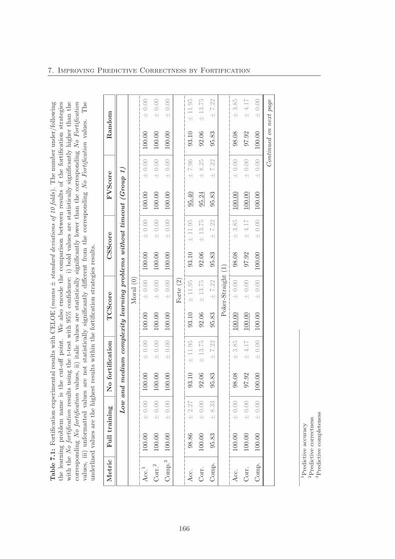
7. Improving Predictive Correctness by Fortification
Table
7.1:Fortificationexperim
entalresultswithCELOE(m
eans±
standard
deviationsof10folds).Thenumber
under/follow
ing
thelearningproblem
nameis
thecut-off
point.
Wealso
encodethecomparison
between
resultsof
thefortification
strategies
withtheNofortification
resultsusingthet-test
with95%
confiden
ce:i)
boldvalues
are
statisticallysignificantlyhigher
thanthe
correspondingNofortification
values,ii)italicvalues
are
statisticallysignificantlylower
thanthecorrespondingNoFortification
values,iii)
unform
atted
values
are
notstatistically
significantly
differentfrom
thecorrespondingNo
Fortification
values.
The
underlined
values
are
thehighestresultswithin
thefortificationstrategiesresults.
Metric
Full
training
Nofortification
TCScore
CSScore
FVScore
Random
Low
and
med
ium
complexitylearn
ingpro
blemswithouttimeo
ut(G
roup
1)
Moral(0)
Acc.1
100.00
±0.00
100.00
±0.00
100.00
±0.00
100.00
±0.00
100.00
±0.00
100.00
±0.00
Corr.2
100.00
±0.00
100.00
±0.00
100.00
±0.00
100.00
±0.00
100.00
±0.00
100.00
±0.00
Comp.3
100.00
±0.00
100.00
±0.00
100.00
±0.00
100.00
±0.00
100.00
±0.00
100.00
±0.00
Forte
(2)
Acc.
98.86
±2.27
93.10
±11.95
93.10
±11.95
93.10
±11.95
95.40
±7.96
93.10
±11.95
Corr.
100.00
±0.00
92.06
±13.75
92.06
±13.75
92.06
±13.75
95.24
±8.25
92.06
±13.75
Comp.
95.83
±8.33
95.83
±7.22
95.83
±7.22
95.83
±7.22
95.83
±7.22
95.83
±7.22
Poker-Straight(1)
Acc.
100.00
±0.00
98.08
±3.85
100.00
±0.00
98.08
±3.85
100.00
±0.00
98.08
±3.85
Corr.
100.00
±0.00
97.92
±4.17
100.00
±0.00
97.92
±4.17
100.00
±0.00
97.92
±4.17
Comp.
100.00
±0.00
100.00
±0.00
100.00
±0.00
100.00
±0.00
100.00
±0.00
100.00
±0.00
Continued
onnextpage
1Predictiveaccuracy
2Predictivecorrectness
3Predictivecompleteness
166

7. Improving Predictive Correctness by Fortification
Table
7.1
–continued
Metric
Full
training
Nofortification
TCScore
CSScore
FVScore
Random
Brother
(0)
Acc.
100.00
±0.00
100.00
±0.00
100.00
±0.00
100.00
±0.00
100.00
±0.00
100.00
±0.00
Daughter(0)
Acc.
100.00
±0.00
100.00
±0.00
100.00
±0.00
100.00
±0.00
100.00
±0.00
100.00
±0.00
Father
(0)
Acc.
100.00
±0.00
100.00
±0.00
100.00
±0.00
100.00
±0.00
100.00
±0.00
100.00
±0.00
Grandson(0)
Acc.
100.00
±0.00
100.00
±0.00
100.00
±0.00
100.00
±0.00
100.00
±0.00
100.00
±0.00
High
and
very
high
complexitylearn
ingpro
blemswithouttimeo
ut(G
roup
2)
Aunt(1)
Acc.
96.5
±0.00
95.25
±8.54
100.00
±0.00
100.00
±0.00
97.75
±0.00
100.00
±0.00
Corr.
95.5
±9.56
90.50
±17.07
100.00
±0.00
100.00
±0.00
97.50
±7.91
100.00
±0.00
Comp.
97.5
±7.91
100.00
±0.00
100.00
±0.00
100.00
±0.00
98.00
±6.33
100.00
±0.00
Cousin(0)
Acc.
99.29
±2.00
99.29
±2.26
99.29
±2.26
99.29
±2.26
99.29
±2.26
99.29
±2.26
Corr.
100.00
±0.00
100.00
±0.00
100.00
±0.00
100.00
±0.00
100.00
±0.00
100.00
±0.00
Comp.
98.57
±4.52
98.57
±4.52
98.57
±4.52
98.57
±4.52
98.57
±4.52
98.57
±4.52
Continued
onnextpage
167
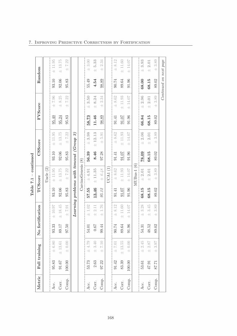
7. Improving Predictive Correctness by Fortification
Table
7.1
–continued
Metric
Full
training
Nofortification
TCScore
CSScore
FVScore
Random
Uncle(2)
Acc.
95.83
±6.80
93.33
±10.97
93.10
±11.95
93.10
±11.95
95.40
±7.96
93.10
±11.95
Corr.
91.67
±13.61
89.17
±18.45
92.06
±13.75
92.06
±13.75
95.24
±8.25
92.06
±13.75
Comp.
100.00
±0.00
97.50
±7.91
95.83
±7.22
95.83
±7.22
95.83
±7.22
95.83
±7.22
Lea
rnin
gpro
blemswith
timeo
ut(G
roup
3)
CarcinoGenesis
(8)
Acc.
53.73
±4.79
54.01
±1.02
57.55
±4.91
56.39
±3.98
58.73
±3.50
55.49
±3.00
Corr.
2.63
±3.40
0.67
±2.11
13.46
±11.35
8.46
±12.13
11.46
±8.24
4.54
±5.33
Comp.
97.22
±7.10
99.44
±1.76
95.12
±6.48
97.28
±5.91
98.89
±2.34
98.89
±2.34
UCA1(1)
Acc.
91.42
±7.01
90.74
±8.12
91.41
±8.62
91.41
±8.62
91.41
±8.62
90.74
±8.12
Corr.
83.39
±13.55
89.64
±11.60
91.07
±11.93
91.07
±11.93
91.07
±11.93
89.64
±11.60
Comp.
100.00
±0.00
91.96
±14.07
91.96
±14.07
91.96
±14.07
91.96
±14.07
91.96
±14.07
MUBus-1(6)
Acc.
53.61
±2.45
54.31
±3.28
68.15
±2.01
78.09
±2.06
66.84
±2.96
68.00
±3.93
Corr.
47.91
±2.87
48.52
±3.45
68.15
±2.01
68.15
±2.01
68.15
±2.01
68.15
±2.01
Comp.
87.71
±3.97
89.02
±3.89
89.02
±3.89
89.02
±3.89
89.02
±3.89
89.02
±3.89
Continued
onnextpage
168
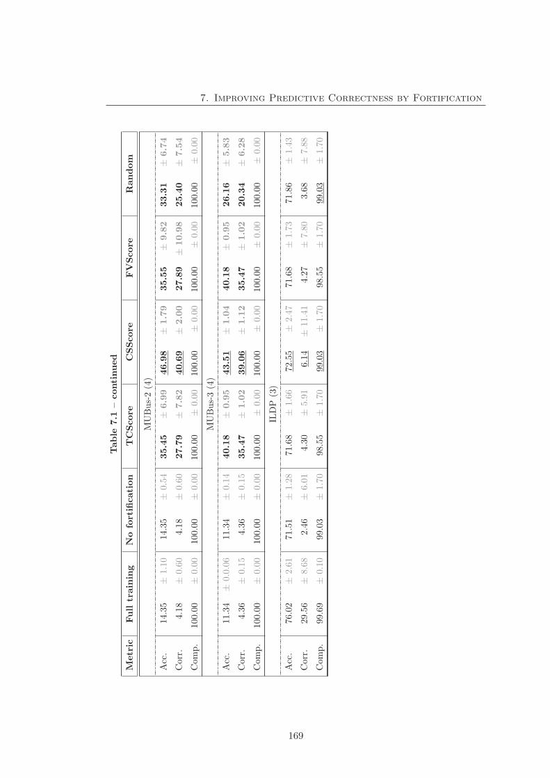
7. Improving Predictive Correctness by Fortification
Table
7.1
–continued
Metric
Full
training
Nofortification
TCScore
CSScore
FVScore
Random
MUBus-2(4)
Acc.
14.35
±1.10
14.35
±0.54
35.45
±6.99
46.98
±1.79
35.55
±9.82
33.31
±6.74
Corr.
4.18
±0.60
4.18
±0.60
27.79
±7.82
40.69
±2.00
27.89
±10.98
25.40
±7.54
Comp.
100.00
±0.00
100.00
±0.00
100.00
±0.00
100.00
±0.00
100.00
±0.00
100.00
±0.00
MUBus-3(4)
Acc.
11.34
±0.0.06
11.34
±0.14
40.18
±0.95
43.51
±1.04
40.18
±0.95
26.16
±5.83
Corr.
4.36
±0.15
4.36
±0.15
35.47
±1.02
39.06
±1.12
35.47
±1.02
20.34
±6.28
Comp.
100.00
±0.00
100.00
±0.00
100.00
±0.00
100.00
±0.00
100.00
±0.00
100.00
±0.00
ILDP
(3)
Acc.
76.02
±2.61
71.51
±1.28
71.68
±1.66
72.55
±2.47
71.68
±1.73
71.86
±1.43
Corr.
29.56
±8.68
2.46
±6.01
4.30
±5.91
6.14
±11.41
4.27
±7.80
3.68
±7.88
Comp.
99.69
±0.10
99.03
±1.70
98.55
±1.70
99.03
±1.70
98.55
±1.70
99.03
±1.70
169
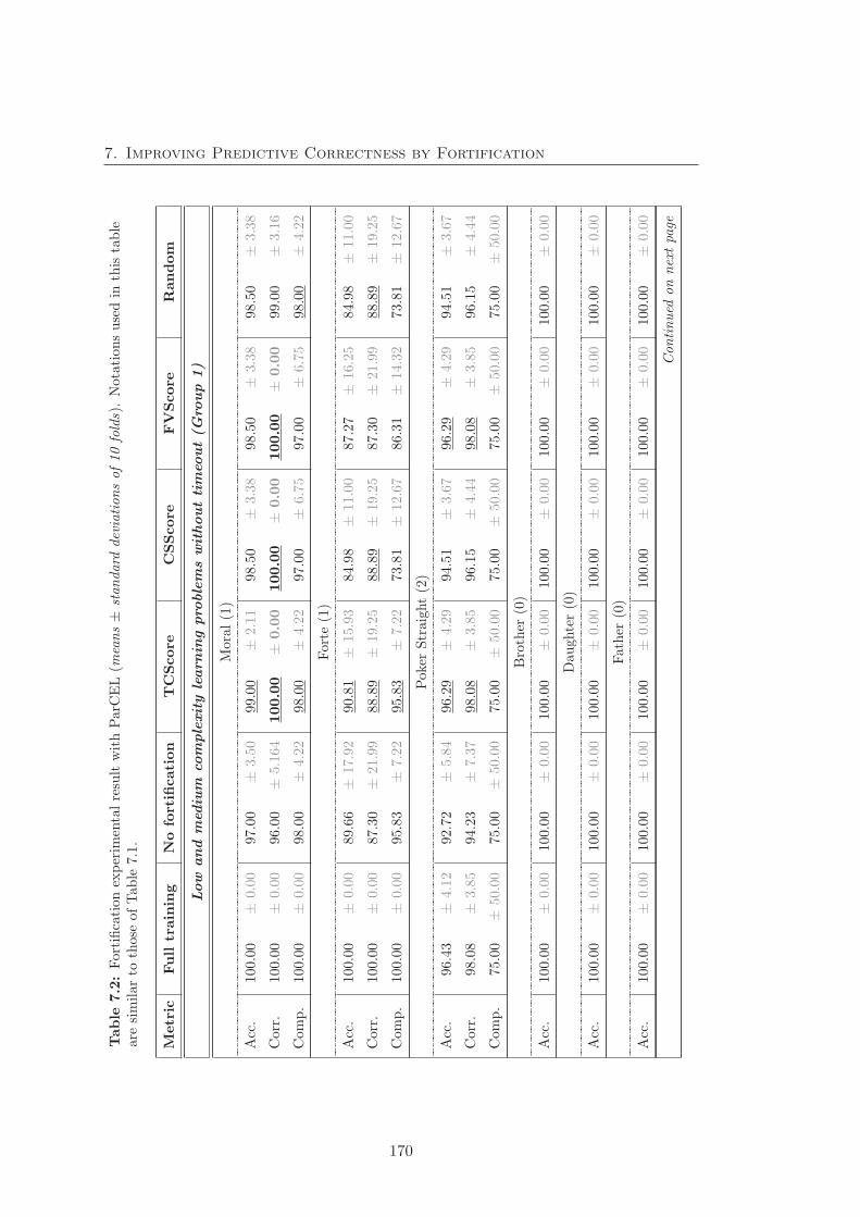
7. Improving Predictive Correctness by Fortification
Table
7.2:Fortificationexperim
entalresultwithParCEL(m
eans±
standard
deviationsof10folds).Notationsusedin
this
table
are
similarto
those
ofTab
le7.1.
Metric
Full
training
Nofortification
TCScore
CSScore
FVScore
Random
Low
and
med
ium
complexitylearn
ingpro
blemswithouttimeo
ut(G
roup
1)
Moral(1)
Acc.
100.00
±0.00
97.00
±3.50
99.00
±2.11
98.50
±3.38
98.50
±3.38
98.50
±3.38
Corr.
100.00
±0.00
96.00
±5.164
100.00
±0.00
100.00
±0.00
100.00
±0.00
99.00
±3.16
Comp.
100.00
±0.00
98.00
±4.22
98.00
±4.22
97.00
±6.75
97.00
±6.75
98.00
±4.22
Forte
(1)
Acc.
100.00
±0.00
89.66
±17.92
90.81
±15.93
84.98
±11.00
87.27
±16.25
84.98
±11.00
Corr.
100.00
±0.00
87.30
±21.99
88.89
±19.25
88.89
±19.25
87.30
±21.99
88.89
±19.25
Comp.
100.00
±0.00
95.83
±7.22
95.83
±7.22
73.81
±12.67
86.31
±14.32
73.81
±12.67
Poker
Straight(2)
Acc.
96.43
±4.12
92.72
±5.84
96.29
±4.29
94.51
±3.67
96.29
±4.29
94.51
±3.67
Corr.
98.08
±3.85
94.23
±7.37
98.08
±3.85
96.15
±4.44
98.08
±3.85
96.15
±4.44
Comp.
75.00
±50.00
75.00
±50.00
75.00
±50.00
75.00
±50.00
75.00
±50.00
75.00
±50.00
Brother
(0)
Acc.
100.00
±0.00
100.00
±0.00
100.00
±0.00
100.00
±0.00
100.00
±0.00
100.00
±0.00
Daughter(0)
Acc.
100.00
±0.00
100.00
±0.00
100.00
±0.00
100.00
±0.00
100.00
±0.00
100.00
±0.00
Father
(0)
Acc.
100.00
±0.00
100.00
±0.00
100.00
±0.00
100.00
±0.00
100.00
±0.00
100.00
±0.00
Continued
onnextpage
170
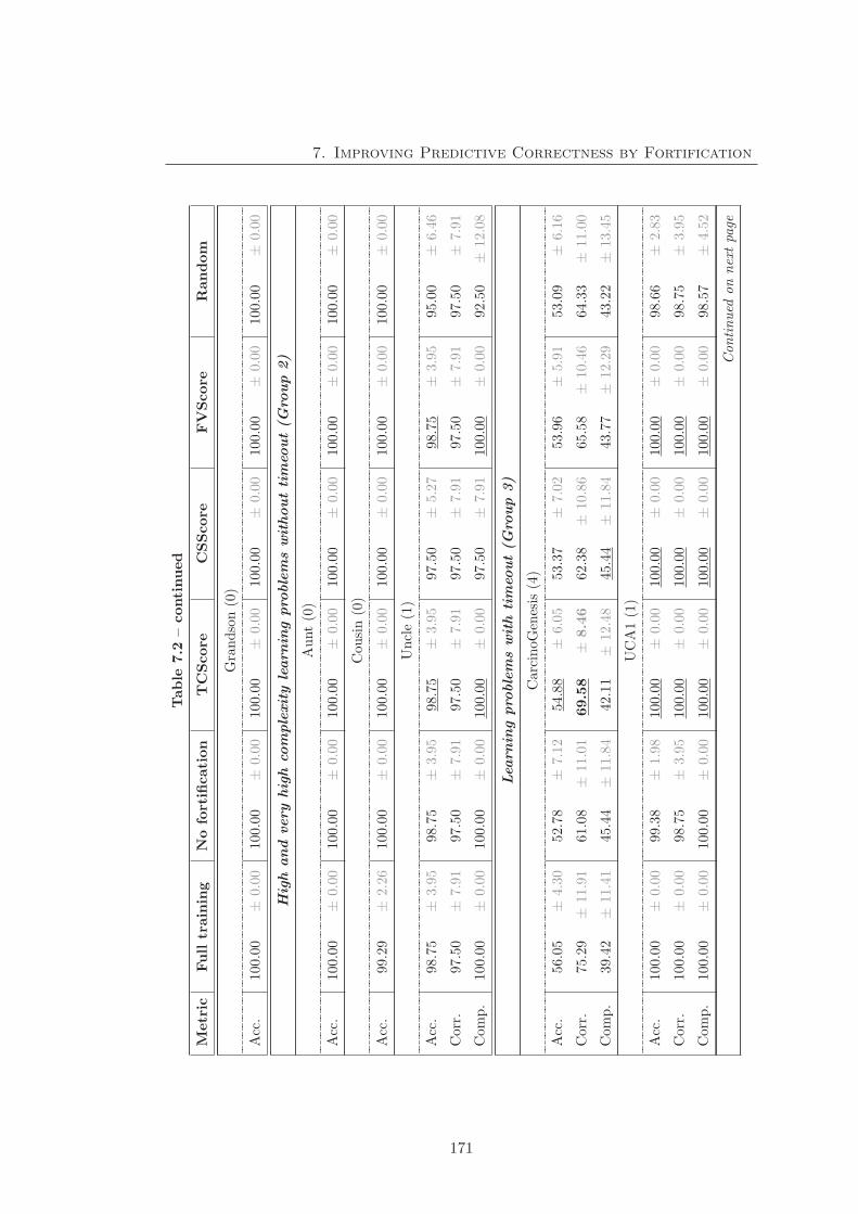
7. Improving Predictive Correctness by Fortification
Table
7.2
–continued
Metric
Full
training
Nofortification
TCScore
CSScore
FVScore
Random
Grandson(0)
Acc.
100.00
±0.00
100.00
±0.00
100.00
±0.00
100.00
±0.00
100.00
±0.00
100.00
±0.00
High
and
very
high
complexitylearn
ingpro
blemswithouttimeo
ut(G
roup
2)
Aunt(0)
Acc.
100.00
±0.00
100.00
±0.00
100.00
±0.00
100.00
±0.00
100.00
±0.00
100.00
±0.00
Cousin(0)
Acc.
99.29
±2.26
100.00
±0.00
100.00
±0.00
100.00
±0.00
100.00
±0.00
100.00
±0.00
Uncle(1)
Acc.
98.75
±3.95
98.75
±3.95
98.75
±3.95
97.50
±5.27
98.75
±3.95
95.00
±6.46
Corr.
97.50
±7.91
97.50
±7.91
97.50
±7.91
97.50
±7.91
97.50
±7.91
97.50
±7.91
Comp.
100.00
±0.00
100.00
±0.00
100.00
±0.00
97.50
±7.91
100.00
±0.00
92.50
±12.08
Lea
rnin
gpro
blemswith
timeo
ut(G
roup
3)
CarcinoGenesis
(4)
Acc.
56.05
±4.30
52.78
±7.12
54.88
±6.05
53.37
±7.02
53.96
±5.91
53.09
±6.16
Corr.
75.29
±11.91
61.08
±11.01
69.58
±8.46
62.38
±10.86
65.58
±10.46
64.33
±11.00
Comp.
39.42
±11.41
45.44
±11.84
42.11
±12.48
45.44
±11.84
43.77
±12.29
43.22
±13.45
UCA1(1)
Acc.
100.00
±0.00
99.38
±1.98
100.00
±0.00
100.00
±0.00
100.00
±0.00
98.66
±2.83
Corr.
100.00
±0.00
98.75
±3.95
100.00
±0.00
100.00
±0.00
100.00
±0.00
98.75
±3.95
Comp.
100.00
±0.00
100.00
±0.00
100.00
±0.00
100.00
±0.00
100.00
±0.00
98.57
±4.52
Continued
onnextpage
171

7. Improving Predictive Correctness by Fortification
Table
7.2
–continued
Metric
Full
training
Nofortification
TCScore
CSScore
FVScore
Random
MUBus-1(3)
Acc.
99.63
±0.31
99.51
±0.47
99.51
±0.47
99.74
±0.36
99.51
±0.47
99.63
±0.47
Corr.
99.61
±0.43
99.52
±0.43
99.52
±0.43
99.78
±0.31
99.52
±0.43
99.69
±0.46
Comp.
99.74
±0.83
99.47
±1.11
99.47
±1.11
99.47
±1.11
99.47
±1.11
99.21
±1.27
MUBus-2(4)
Acc.
97.91
±0.50
98.05
±0.57
98.12
±0.53
98.26
±0.61
98.12
±0.53
98.08
±0.59
Corr.
99.54
±0.45
99.49
±0.24
99.56
±0.24
99.72
±0.25
99.56
±0.24
99.52
±0.27
Comp.
84.18
±5.59
85.97
±6.26
85.97
±6.26
85.97
±6.26
85.97
±6.26
85.97
±6.26
MUBus-3(3)
Acc.
95.85
±0.31
94.57
±0.32
94.65
±0.32
94.65
±0.32
94.65
±0.32
94.58
±0.33
Corr.
99.74
±0.17
99.86
±0.05
99.94
±0.06
99.94
±0.06
99.94
±0.06
99.88
±0.05
Comp.
46.40
±3.66
27.36
±4.48
27.36
±4.48
27.36
±4.48
27.36
±4.48
27.28
±4.39
ILDP
(2)
Acc.
71.12
±5.36
70.24
±6.76
72.07
±6.86
69.22
±5.66
72.06
±7.01
69.84
±5.95
Corr.
29.56
±8.68
67.28
±12.74
74.49
±12.42
67.90
±12.98
74.49
±12.42
69.15
±11.59
Comp.
99.69
±0.10
71.80
±11.32
70.87
±11.40
69.93
±10.51
70.86
±11.42
70.25
±10.10
172
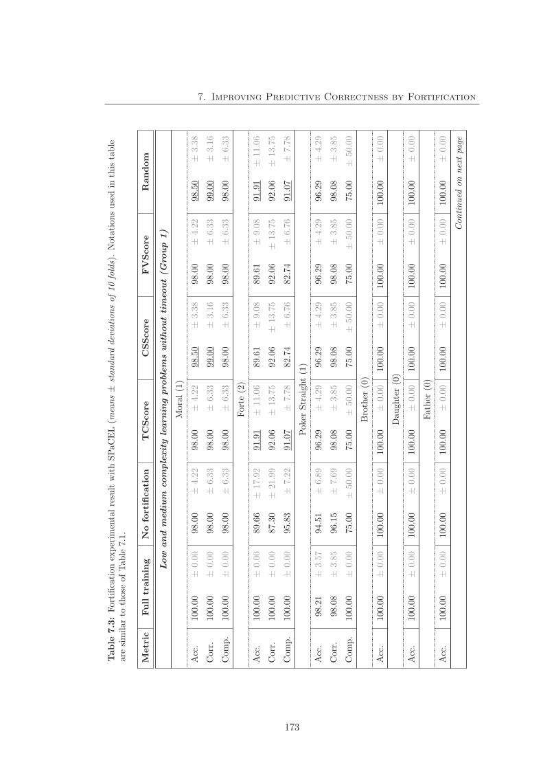
7. Improving Predictive Correctness by Fortification
Table
7.3:Fortificationexperim
entalresultwithSPaCEL(m
eans±
standard
deviationsof10folds).Notationsusedin
thistable
are
similarto
those
ofTab
le7.1.
Metric
Full
training
Nofortification
TCScore
CSScore
FVScore
Random
Low
and
med
ium
complexitylearn
ingpro
blemswithouttimeo
ut(G
roup
1)
Moral(1)
Acc.
100.00
±0.00
98.00
±4.22
98.00
±4.22
98.50
±3.38
98.00
±4.22
98.50
±3.38
Corr.
100.00
±0.00
98.00
±6.33
98.00
±6.33
99.00
±3.16
98.00
±6.33
99.00
±3.16
Comp.
100.00
±0.00
98.00
±6.33
98.00
±6.33
98.00
±6.33
98.00
±6.33
98.00
±6.33
Forte
(2)
Acc.
100.00
±0.00
89.66
±17.92
91.91
±11.06
89.61
±9.08
89.61
±9.08
91.91
±11.06
Corr.
100.00
±0.00
87.30
±21.99
92.06
±13.75
92.06
±13.75
92.06
±13.75
92.06
±13.75
Comp.
100.00
±0.00
95.83
±7.22
91.07
±7.78
82.74
±6.76
82.74
±6.76
91.07
±7.78
Poker
Straight(1)
Acc.
98.21
±3.57
94.51
±6.89
96.29
±4.29
96.29
±4.29
96.29
±4.29
96.29
±4.29
Corr.
98.08
±3.85
96.15
±7.69
98.08
±3.85
98.08
±3.85
98.08
±3.85
98.08
±3.85
Comp.
100.00
±0.00
75.00
±50.00
75.00
±50.00
75.00
±50.00
75.00
±50.00
75.00
±50.00
Brother
(0)
Acc.
100.00
±0.00
100.00
±0.00
100.00
±0.00
100.00
±0.00
100.00
±0.00
100.00
±0.00
Daughter(0)
Acc.
100.00
±0.00
100.00
±0.00
100.00
±0.00
100.00
±0.00
100.00
±0.00
100.00
±0.00
Father
(0)
Acc.
100.00
±0.00
100.00
±0.00
100.00
±0.00
100.00
±0.00
100.00
±0.00
100.00
±0.00
Continued
onnextpage
173

7. Improving Predictive Correctness by Fortification
Table
7.3
–continued
Metric
Full
training
Nofortification
TCScore
CSScore
FVScore
Random
Grandson(0)
Acc.
100.00
±0.00
100.00
±0.00
100.00
±0.00
100.00
±0.00
100.00
±0.00
100.00
±0.00
High
and
very
high
complexitylearn
ingpro
blemswithouttimeo
ut(G
roup
2)
Aunt(1)
Acc.
100.00
±0.00
98.75
±3.95
98.75
±3.95
98.75
±3.95
98.75
±3.95
97.75
±4.78
Corr.
100.00
±0.00
97.50
±7.91
97.50
±7.91
100.00
±0.00
97.50
±7.91
97.50
±7.91
Comp.
100.00
±0.00
100.00
±0.00
100.00
±0.00
97.50
±7.91
100.00
±0.00
98.00
±6.33
Cousin(0)
Acc.
100.00
±0.00
97.32
±5.66
97.32
±5.66
97.32
±5.66
97.32
±5.66
97.32
±5.66
Corr.
100.00
±0.00
94.64
±11.33
94.64
±11.33
94.64
±11.33
94.64
±11.33
94.64
±11.33
Comp.
100.00
±0.00
100.00
±0.00
100.00
±0.00
100.00
±0.00
100.00
±0.00
100.00
±0.00
Uncle(1)
Acc.
95.42
±10.84
95.83
±6.80
98.33
±5.27
94.58
±7.10
97.08
±6.23
94.58
±7.10
Corr.
90.83
±21.68
91.67
±13.61
96.67
±10.54
94.17
±12.45
96.67
±10.54
91.67
±13.61
Comp.
100.00
±0.00
100.00
±0.00
100.00
±0.00
95.00
±10.54
97.50
±7.91
97.50
±7.91
Lea
rnin
gpro
blemswith
timeo
ut(G
roup
3)
CarcinoGenesis
(7)
Acc.
60.52
±6.06
56.36
±7.22
57.24
±6.33
57.85
±5.87
57.57
±8.56
56.63
±9.07
Corr.
35.42
±8.39
43.25
±10.32
53.50
±5.45
50.33
±5.87
51.00
±9.57
47.75
±12.30
Comp.
81.90
±6.77
67.54
±10.05
60.32
±11.36
64.27
±9.12
63.13
±9.96
64.21
±12.25
Continued
onnextpage
174
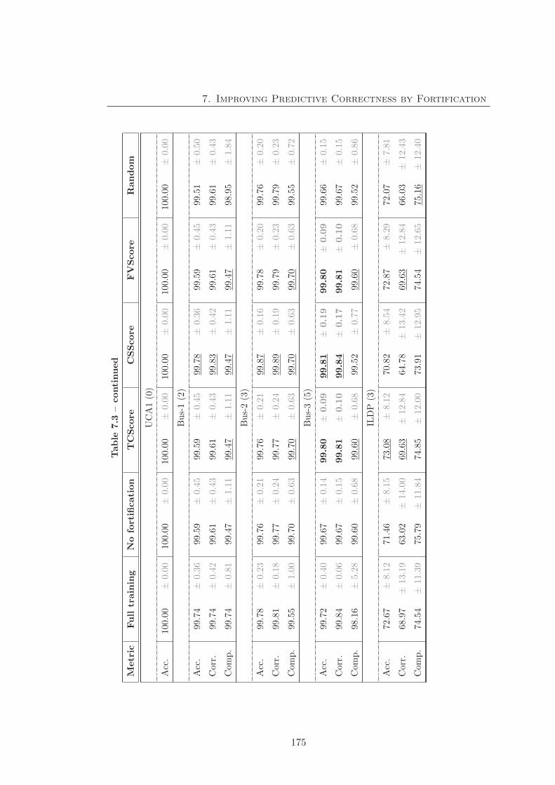
7. Improving Predictive Correctness by Fortification
Table
7.3
–continued
Metric
Full
training
Nofortification
TCScore
CSScore
FVScore
Random
UCA1(0)
Acc.
100.00
±0.00
100.00
±0.00
100.00
±0.00
100.00
±0.00
100.00
±0.00
100.00
±0.00
Bus-1(2)
Acc.
99.74
±0.36
99.59
±0.45
99.59
±0.45
99.78
±0.36
99.59
±0.45
99.51
±0.50
Corr.
99.74
±0.42
99.61
±0.43
99.61
±0.43
99.83
±0.42
99.61
±0.43
99.61
±0.43
Comp.
99.74
±0.81
99.47
±1.11
99.47
±1.11
99.47
±1.11
99.47
±1.11
98.95
±1.84
Bus-2(3)
Acc.
99.78
±0.23
99.76
±0.21
99.76
±0.21
99.87
±0.16
99.78
±0.20
99.76
±0.20
Corr.
99.81
±0.18
99.77
±0.24
99.77
±0.24
99.89
±0.19
99.79
±0.23
99.79
±0.23
Comp.
99.55
±1.00
99.70
±0.63
99.70
±0.63
99.70
±0.63
99.70
±0.63
99.55
±0.72
Bus-3(5)
Acc.
99.72
±0.40
99.67
±0.14
99.80
±0.09
99.81
±0.19
99.80
±0.09
99.66
±0.15
Corr.
99.84
±0.06
99.67
±0.15
99.81
±0.10
99.84
±0.17
99.81
±0.10
99.67
±0.15
Comp.
98.16
±5.28
99.60
±0.68
99.60
±0.68
99.52
±0.77
99.60
±0.68
99.52
±0.86
ILDP
(3)
Acc.
72.67
±8.12
71.46
±8.15
73.08
±8.12
70.82
±8.54
72.87
±8.29
72.07
±7.81
Corr.
68.97
±13.19
63.02
±14.00
69.63
±12.84
64.78
±13.42
69.63
±12.84
66.03
±12.43
Comp.
74.54
±11.39
75.79
±11.84
74.85
±12.00
73.91
±12.95
74.54
±12.65
75.16
±12.40
175

7. Improving Predictive Correctness by Fortification
7.5 Conclusion
This chapter has presented a fortification method for improving the predictive accu-
racy of the class expression learning algorithms. A fortification method consists of
a method for generating the fortifying definition, a fortification scoring and a cut-off
point computation strategies.
This chapter has also provided one method for fortifying definition generation, three
fortification scoring methods and one cut-off point computation strategy. Overall, the
experimental results in Tables 7.1, 7.2 and 7.3 show that this method improved the
predictive predictive accuracy of most learning problems in the experiments. This
means that the predictive accuracy was increased and the increase of the predictive
correctness was higher than the decrease of the completeness (if any).
The experiments were conducted on three learning algorithms that use three dif-
ferent class expression learning approaches. The experimental results of CELOE and
ParCEL were better than those of SPaCEL: 14/30 results of CELOE and 8/30 results
of ParCEL were above the baseline in comparison with 6/33 results of SPaCEL. One
of the possible reasons is that CELOE and ParCEL had better fortifying definitions
for fortification than SPaCEL. In SPaCEL, some of the fortifying definitions were used
to construct the learnt concept (counter-partial definitions) and they may be the most
promising definitions for the fortification.
Amongst the three fortification strategies, CSScore produced better results in more
learning problems than TCScore and FVScore. However, the TCScore strategy does not
require an additional step to compute the fortification score. The result of the random
fortifying definition selection was also presented in Tables 7.1, 7.2 and 7.3. The results
illustrates the positive effect of the fortification strategies on the fortification result.
The random selection strategy gave lower accuracy than the other strategies in more
learning problems.
The current cut-off point computation strategy produced promising results. The
increase of predictive correctness that was caused by the fortification was higher than
the decrease of predictive completeness in most of learning problems in the experiments.
As a result, the predictive accuracy also increased. There was no significant decrease
176
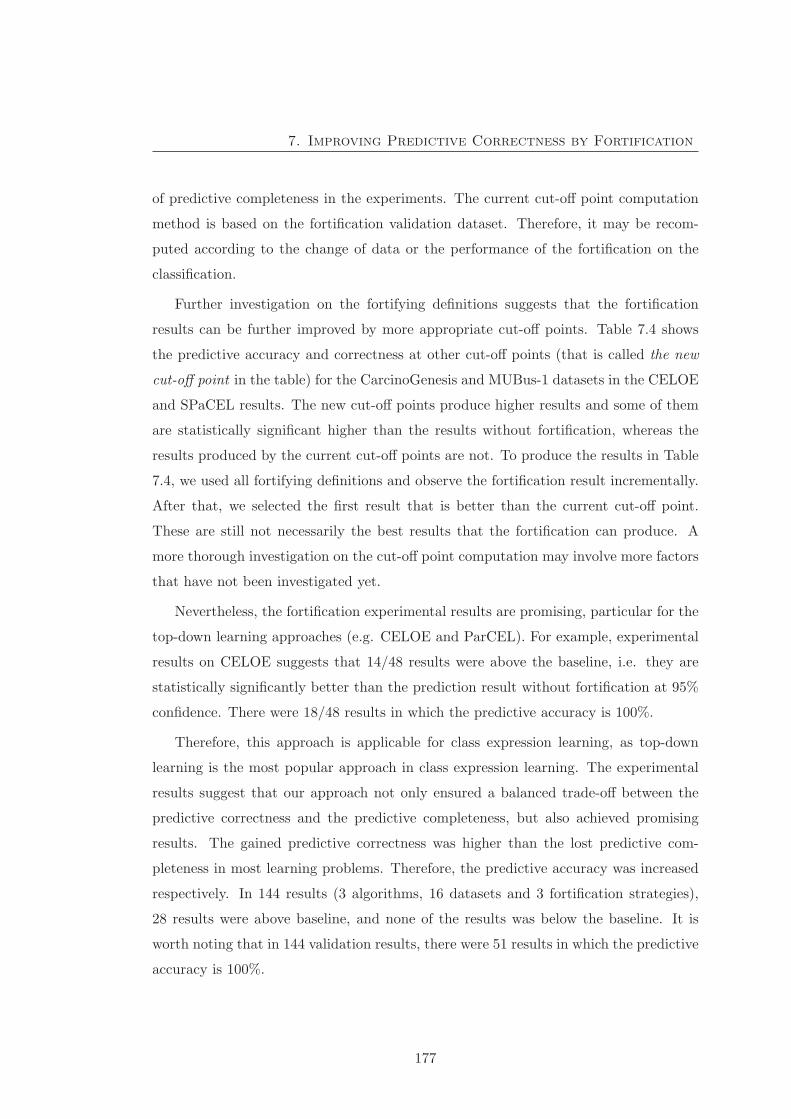
7. Improving Predictive Correctness by Fortification
of predictive completeness in the experiments. The current cut-off point computation
method is based on the fortification validation dataset. Therefore, it may be recom-
puted according to the change of data or the performance of the fortification on the
classification.
Further investigation on the fortifying definitions suggests that the fortification
results can be further improved by more appropriate cut-off points. Table 7.4 shows
the predictive accuracy and correctness at other cut-off points (that is called the new
cut-off point in the table) for the CarcinoGenesis and MUBus-1 datasets in the CELOE
and SPaCEL results. The new cut-off points produce higher results and some of them
are statistically significant higher than the results without fortification, whereas the
results produced by the current cut-off points are not. To produce the results in Table
7.4, we used all fortifying definitions and observe the fortification result incrementally.
After that, we selected the first result that is better than the current cut-off point.
These are still not necessarily the best results that the fortification can produce. A
more thorough investigation on the cut-off point computation may involve more factors
that have not been investigated yet.
Nevertheless, the fortification experimental results are promising, particular for the
top-down learning approaches (e.g. CELOE and ParCEL). For example, experimental
results on CELOE suggests that 14/48 results were above the baseline, i.e. they are
statistically significantly better than the prediction result without fortification at 95%
confidence. There were 18/48 results in which the predictive accuracy is 100%.
Therefore, this approach is applicable for class expression learning, as top-down
learning is the most popular approach in class expression learning. The experimental
results suggest that our approach not only ensured a balanced trade-off between the
predictive correctness and the predictive completeness, but also achieved promising
results. The gained predictive correctness was higher than the lost predictive com-
pleteness in most learning problems. Therefore, the predictive accuracy was increased
respectively. In 144 results (3 algorithms, 16 datasets and 3 fortification strategies),
28 results were above baseline, and none of the results was below the baseline. It is
worth noting that in 144 validation results, there were 51 results in which the predictive
accuracy is 100%.
177
7. Improving Predictive Correctness by Fortification
Table 7.4: Experimental results for new cut-off points (means ± standard deviations of10 folds). The pairs of numbers below the learning problem names represent the current(Old) and the new (New) cut-off points respectively. The representation conventions aresimilar to Table 7.1. “No fort.” is the abbreviation for “No fortification”.
Problem MetricNofort.
TCScore CSScore FVScore
Old New Old New Old New
ParCEL
CarcinoGenesis(8, 5)
Acc. 52.78±7.12
54.88±6.38
54.55±6.31
53.08±6.83
54.57±5.05
54.25±6.70
53.98±4.88
Corr. 61.08±11.01
69.58±8.46
73.46±6.82
62.38±10.86
68.83±8.75
65.58±10.46
70.83±10.81
MUBus-1(6, 16)
Acc. 99.51±0.47
99.51±0.47
99.78±0.26
99.74±0.36
99.78±0.26
99.51±0.47
99.78±0.26
Corr. 99.52±0.43
99.52±0.43
99.83±0.23
99.78±0.31
99.96±0.14
99.52±0.43
99.83±0.23
SPaCEL
MUBus-1(2, 21)
Acc. 99.59±0.45
99.59±0.45
99.89±0.18
99.78±0.36
99.81±0.26
99.59±0.45
99.85±0.19
Corr. 99.61±0.43
99.61±0.43
99.96±0.14
99.83±0.42
99.91±0.28
99.61±0.43
99.91±0.18
MUBus-2(2, 21)
Acc. 99.76±0.21
99.76±0.21
99.83±0.20
99.87±0.16
99.94±0.08
99.78±0.20
99.83±0.20
Corr. 99.77±0.24
99.77±0.24
99.84±0.23
99.89±0.19
99.97±0.08
99.79±0.23
99.84±0.23
178
7. Improving Predictive Correctness by Fortification
In the three fortification scoring strategies, the TCScore strategy does not require
additional computation and dataset to score the fortification candidates. Therefore, it
is suitable for learning problems that do not have enough additional data for scoring.
This strategy is also suitable for learning problems where the training data contains
enough information to describe the scenario.
On the other hand, CSSccore and FVScore require additional computation and a
validation dataset. As these strategies use a separate dataset for scoring, they can
deal with the unseen characteristics in the training data, i.e. incomplete training data.
CSScore also uses the similarity between concepts to score the candidates. Therefore,
it often had stronger impact on the fortification results. Using both ABox and TBox
in scoring the candidates also help this strategy to be less dependant on the additional
dataset. If there is no additional dataset, it can be adjusted to use only the TBox. In
comparison with the TCScore and FVScore that use only the ABox, the combination
of both ABox and TBox of the CSScore produced better results.
As each of the strategies uses different aspects to score the candidates, e.g. TCScore
employs the training model, and CSScore employs the concept model (TBox) and a
validation model (similarity based on ABox), a combination of them may create a
potential scoring strategy. This is left as future work.
179

7. Improving Predictive Correctness by Fortification
180

Chapter 8
Conclusions and Future Work
In this chapter, we first summarise the results and contributions of the thesis.
Then, we point out potential threats to the validity of results and discuss
future work.
8.1 Discussion and Contributions of the Thesis
This thesis proposes novel approaches in description logic learning to improve speed
and scalability, and to provide flexibility to trade off between predictive correctness and
predictive completeness.
Two approaches have been proposed to speed up learning and improve the ability
of the learning algorithms to deal with complex learning problems. In the first ap-
proach, the Parallel Class Expression Learning (ParCEL) algorithm, the learning is
sped up by increasing the number of computations of the learning algorithm in a unit
of time. The approach uses parallelisation to take advantage of multi-core processors
and multi-processor systems. Moreover, the implicit divide and conquer strategy be-
hind the three-step learning approach, which combines both top-down and bottom-up
learning and a reduction step, helps to increase the scalability of the learning algo-
rithm when the complexity of the learning problems increases. The reduction step
enables customisation of the learnt models, i.e. to create bias towards a certain metric
such as total definition length or the number of sub-solutions. The experiments show
181
8. Conclusions and Future Work
promising results for both learning time and the ability to deal with complex learning
problems. The results were compared with the Class Expression Learner for Ontology
Engineering algorithm (CELOE), a top-down OWL class expression learning that was
recently developed. The experimental results show that ParCEL outperformed CELOE
on most learning problems in the experiments. The ParCEL approach addresses the
second objective of the research and it was presented in Chapter 5.
A Symmetric Class Expression Learning (SPaCEL) approach has also been intro-
duced to improve learning speed. The idea underlying this approach is to reduce the
number of computations necessary to find the solution. This objective was achieved
by using downward refinement to build models for both positive and negative exam-
ples simultaneously. In other words, the approach utilises definitions of both positive
and negative examples. The downward refinement operators for description logics are
not dedicated to finding the definition of positive or negative examples. They simply
specialise a given description and therefore refinement results may be the definitions of
positive or negative examples. Most top-down learning approaches only seek a defini-
tion for positive examples and they are completely based on the refinement operators.
However, models of positive examples can be constructed using the models of neg-
ative examples. For instance, the concept Father can be defined not only as Male
AND hasChild SOME Person but also as hasChild SOME Person AND (not Female)
where Female is a model of negative examples. Intuitively, a symmetric approach can
use the refinement results more effectively and thus can reduce the search space size.
In addition, this approach is also beneficial for parallelisation. The evaluation results
suggest that combining these methods reduced the search space significantly in com-
parison with CELOE, a top-down class expression learning algorithm. The SPaCEL
approach addresses the third objective of the research and it was presented in Chapter
6.
An Adaptive Numerical Data Segmentation approach that aims to segment the
values of numerical datatype properties to add support for numerical data learning
in description logic learning has been introduced. This approach contributes to the
improvement of the scalability and speed of description logic learning. We have shown
that this approach computes quasi-order sets for refinement of numerical datatype
182
8. Conclusions and Future Work
properties based on relational graphs that describe relationships between examples and
the values of datatype property assertions. The relational graphs provide necessary
information to reduce redundancy and avoid the missing of any necessary values in
the quasi-order space. As the result, this approach decreases the learning search space
and speeds up the learning algorithms. The Adaptive Numerical Data Segmentation
approach addresses the first objective of our research and it was presented in Chapter
4.
To provide flexibility to trade off between predictive correctness and predictive
completeness, fortification of the prediction model has been proposed. In description
logic learning, the top-down approach is most used and it tends to create bias towards
predictive completeness. Therefore, a method that can improve predictive correctness
to provide flexibility to trade off between these factors has been proposed. The basic
idea of this approach is to fortify the predictive correctness by applying a level of over-
specialisation on the prediction model. Two questions in this problem were addressed:
i) how to specialise the prediction model, and ii) how much specialisation should be
applied.
A method for producing fortification candidates has been proposed that can be
applied to arbitrary class expression learning algorithms. Fortification candidates can
be computed by swapping the sets of positive and negative examples and using the
allowed noise percentage in the learning setting. More over-specialisation can poten-
tially provide higher prediction correctness, but it can lead to over-fitting. Therefore,
methods for ranking the fortification candidates and identifying appropriate levels of
over-specialisation for the prediction model have been proposed. Three ranking meth-
ods have been proposed, based respectively on training coverage, fortification validation
and concept similarity. These methods use different aspects to rank the candidates and
thus each of them is suitable for a particular class of problems. The number of candi-
dates used for fortification, called cut-off point, is computed based on the fortification
validation dataset.
The experiments show promising results, particularly on top-down learning ap-
proaches such as CELOE and ParCEL. However, further investigation suggests that
the proposed cut-off strategy is not optimal. The fortification results could be further
183
8. Conclusions and Future Work
improved by a more appropriate cut-off point computation strategy. The Fortification
Approach to Improve Predictive Correctness addresses the fourth objective of the thesis
and it was described in Chapter 7.
In addition to the above-mentioned findings, this thesis also produced some other
considerable contributions. Two learners, ParCEL and SPaCEL, and a fortification
model were implemented and integrated into DL-Learner, a popular description logic
learning framework1 (see Appendix A). In addition, an evaluation methodology that
was designed in Chapter 3 includes all aspects of a thorough evaluation: selection
of datasets; evaluation metrics; measurement methodology and statistical significance
tests. An overview of the literature in the field of class expression learning was also
provided in Chapter 2.
8.2 Threats to Validity of the Results
In this section, we discuss the uncontrollable factors that impact on the results of
the experiments (internal validity) and the generalisability of the findings (external
validity).
8.2.1 Threats to internal validity
Four potential threats to the internal validity of the experimental results have been
identified:
1. Thread scheduling. Class expression learning is essentially a search problem
where the exploration of the search space is controlled by a search heuristics. In
parallel class expression learning, multiple workers are used to explore the search
space (search tree) simultaneously. Although the descriptions in the search space
(branches) are assigned to the workers based on the search heuristic, the order of
refinements may be slightly different between different runs of the same learning
problem depending on the order in which the workers are scheduled. Potential
metrics affected by this threat are the learning time and the predictive accuracy.
Our investigation suggested that there was not a significant variation between
1http://dl-learner.svn.sourceforge.net/viewvc/dl-learner/
184

8. Conclusions and Future Work
runs. However, this does not mean that the threat caused by thread scheduling
can be completely ignored. It can be addressed by using the multi-run k-fold
cross-validation method.
2. Concurrency control. In a parallel programming paradigm, concurrency con-
trol between threads is an important issue. In our implementation, monitor locks
(i.e. synchronized blocks) and concurrent data structures were used for con-
currency control [25, 47, 136]. While the concurrent data structures allow for
higher guarantees of concurrency control, the monitoring locks have the poten-
tial to cause conflicts between threads. Using concurrency is a trade-off between
avoiding concurrency-related problems such as deadlocks and taking advantage of
parallelism. Our implementation might not strike the optimal balance, affecting
the learning time and accuracy.
3. Calibration of problems. In general, default learning configurations suggested
by the learners were always used (see [82] for CELOE settings and Chapters 6
for ParCEL and SPaCEL settings). However, other settings may yield better
results. In particular, there are two basic learning settings that influence the
learning results: the allowed noise percentage and the search heuristic. The first
setting is very important to deal with the noisy learning problems. In our ex-
periments, CarcinoGenesis and ILDP are noisy datasets. It was reported that
CELOE achieved the highest accuracy on the CarcinoGenesis dataset when the
allowed noise percentage is 30% [82]. Similarly, the learning heuristic is also a
potential factor that influences the experimental results. Appropriate learning
heuristics can help to improve the learning time and perhaps the predictive ac-
curacy. For example, the solution for a complex learning problem can be found
faster if the penalty on the description length is low or vice versa.
There are two reasons for using the default learning setting in our experiments.
First, investigating this cracks the combinatorial exploration of a problem that is
already computationally expensive. Second, it is necessary to avoid the favouritism
between learning algorithms that is caused by the customised learning configura-
tions. For example, we may set an inappropriate penalty factor for the comparison
185
8. Conclusions and Future Work
algorithm while optimising this factor for our algorithm. Therefore, if the exper-
imental results are used to compare between learners, the impact of this threat
upon the results will not be significant. Otherwise, this threat should be treated
with caution. It can be counteracted by using a validation dataset to investigate
the best learning setting.
8.2.2 Threats to external validity
Two threats that potentially influence the generalisability of the findings should be
considered:
1. Implementation language selection bias. Our algorithms have been imple-
mented in Java, which is widely used by the Semantic Web community. Therefore,
it can benefit the implementation of existing semantic web techniques such as the
application programming interface for OWL (OWLAPI) and the OWL reason-
ers. This language also strongly supports concurrency control techniques that
are necessary for implementing parallelisation. However, the more benefits the
implementation got, the more difficult the migration of the implementation would
be. In the context of the Semantic Web application, the influence of this threat
to validity of our implementation is not a major concern. Therefore, we consider
it as a minor threat to the external validity of our implementation.
2. Dataset and reasoning framework selection. The low to high complexity
datasets, whose definitions have from several to hundreds of axioms, were used
for evaluation. However, the size of these datasets ranges only from small to
medium. Therefore, this allows the entire knowledge base of the learning problems
to be loaded into memory and reasoner for processing and reasoning. In real-
world applications, there are many large to very large ontologies that contain
thousands to hundred thousands of classes and properties such as DBpedia, Cyc,
etc. [18, 94]. Our algorithms cannot be applied directly to learning problems
with such knowledge bases. The reason for this issue is that the OWL reasoners
used in our algorithms, Pellet [107] and Fast Instance Check (FIC) [81], cannot
load the entirety of the large ontologies into memory for reasoning. The initial
186
8. Conclusions and Future Work
time for loading and classifying such ontologies is time-consuming. This can
be considered a major threat for our algorithms as the learning problems are
increasing not only in term of complexity (of the definitions) but also in term
of size (of the knowledge base). A potential solution for this problem is to use
the knowledge fragment selection approach [58, 116], which allows the reasoning
to be performed within a ‘related part’ of the knowledge base towards a given
reasoning request. Another solution is to use the parallel semantic web reasoning
frameworks that are developed for web-scale knowledge bases such as LarKC [48],
Reasoning-Hadoop [132] and WebPIE [131].
8.3 Future Work
Our experiments achieved promising results in improving class expression learning al-
gorithms’ performance and providing a flexible trade-off between predictive correctness
and completeness. However, our investigations have shown that there are other inter-
esting properties that have not been explored yet.
It would be useful to test the learning algorithms with more learning problems,
particularly learning problems with large knowledge bases and noisy datasets. This
would provide more thorough investigations into the ability of the learning algorithms
to deal with large knowledge bases and noisy datasets, which would help improve the
algorithms’ applicability for real-world applications. This is a challenging work as
handling noisy data is a difficult problem in machine learning.
The second direction is to investigate more reduction strategies for the Parallel
Class Expression Learning algorithm. The current reduction strategies are based on
the greedy strategy combined with a scoring criteria that creates bias towards certain
metrics. Each of the current reduction strategies uses only one certain condition to score
the partial solutions such as training coverage or definition length. Of a partial solution,
these two basic attributes are currently used separately. However, a combination of
these metrics may result in a more promising reduction strategy. For example, consider
two partial definitions with length 5 where each of them covers 80% of the positive
examples and their combination covers 100% of the positive examples. The combination
187
8. Conclusions and Future Work
of these partial definitions is preferred to a definition with length 15 that has 100%
coverage. However, a definition with length 15 that covers 100% of the positive examples
is better than 3 partial definitions with length 10 where each of them covers 40% and
their combination covers 100% of the positive examples. This example implies that a
more thorough reduction strategy requires the combination of different metrics.
Another direction that is also related to the construction of the final definition is
the normalisation and simplification of the learnt definitions. As discussed in Section
6.3.4, the current partial definition aggregation simply creates disjunction of all reduced
partial definitions. This may produce redundancies in the final definition, particularly
in the SPaCEL approach, where the counter-partial definitions can be used in many
partial definitions. Optimisation and simplification can be used to optimise and simplify
descriptions in description logics [3, 65]. They can remove redundancy in the learnt
definitions to reduce their length and increase the readability.
Fortification scoring and cut-off point estimation strategies can also be improved
further. An initial investigation into the experimental results in Section 7.5 shows
that although the current fortification and cut-off point estimation strategies produce
promising results, they have potential to produce even more promising results. Each of
the current fortification scoring strategies is based on a certain aspect such as training
coverage and concept similarity. A combination of these aspects can result in a more
robust strategy. In addition, a cut-off point strongly influences the fortification results.
The current strategy uses a fortification validation dataset for estimating the cut-off
points. However, a combination with training accuracy, completeness and correctness
may produce a better strategy.
Improving the scalability of the learner with respect to the size of the learning prob-
lem’s knowledge base is an indispensable direction to help the learners to be more useful
for real-word applications. As was explained in the discussion of potential threats to ex-
ternal validity of the research (see Section 8.2.2), there are two possible approaches for
this direction. The first approach is to use more scalable reasoning frameworks for the
learners, particularly the parallel and web-scale reasoners frameworks such as LarKC
[48], Reasoning-Hadoop [132] and WebPIE [131]. Another approach is to use the knowl-
edge fragment selection technique to reduce the size of the knowledge base required for
188
8. Conclusions and Future Work
instances checks [58, 116]. This technique identifies a minimal segment of knowledge
base that is relevant to the instance checks of a learning problem. This approach is
particularly useful for learning problems that use the general (upper) ontologies as the
knowledge base.
Another potential direction for future work is to redesign the learner to enable
the use of cloud computing [1, 23, 41]. An advantage for this direction is that the
current learners use the map-reduce architecture. This model is used for most cloud
technologies such as Hadoop [138] and CGL-MapReduce [42]. However, as with other
parallel and distributed algorithms, dealing with the concurrency and latency between
nodes in the cloud is the most challenging problem. The latency between cloud nodes
may influence the learnt result as it may influence the learning heuristics’ impact.
However, this direction, together with the improvement of the reasoning scalability, will
result in a highly scalable class expression learner that can handle learning problems
that have web-scale knowledge bases.
189

8. Conclusions and Future Work
190
Appendix A
Accessing the Implementation
The algorithms proposed in this thesis including ParCEL, SPaCEL and Fortification
for description logic learning are implemented based on the DL-Learner, an open source
machine learning framework [79]. This appendix first introduces briefly the DL-Learner
framework architecture based on its manual. After that, we present structure of the
algorithms proposed in this thesis. Finally, we provide instructions for checking out
and compiling the projects.
A.1 Software Structure
Our algorithms are implemented based on DL-Learner framework. This is an open
source Web Ontology Language learning framework developed by Lehmann and his
team [79]. It is written in Java and developed using Maven software project man-
agement architecture [92]. It provides flexibility for developing and new description
learning algorithms and integrating them into this framework as it uses the component
based model.
A.1.1 DL-Learner architecture
The architecture of this framework is adopted from [79] as shown in Figure A.1. There
are four core components:
Knowledge source – is a wrapper for knowledge bases and provides interface for ac-
191

A. Accessing the Implementation
cessing data inside the knowledge bases. This component is used by reasoner com-
ponents. Some types of knowledge sources currently supported by this framework
are OWL files (in various syntax), SPARQL endpoints and linked data [17, 29].
Reasoning component – provides reasoning services on knowledge sources to the
learning algorithm and learning problem components. It supports DIG 1.1 [10]
and OWLAPI [11] reasoner interfaces to connect to most of OWL reasoners such
as Pellet, FaCT and Hermit.
Learning problem – specifies types of learning problem (see Section 2.2 for more
details) accompanying the necessary information to describe a learning problem,
e.g. sets of positive and negative examples. This component also provides cal-
culations related to the learning problem such as completeness, correctness and
accuracy.
Learning algorithm – provides methods to solve one or more types of learning prob-
lem. The relation between this component and other components is illustrated in
Figure A.1.
This framework also provide interfaces (graphical and command line) for running
and interacting with the learning algorithm. More details can be found in [79].
A.1.2 Our algorithms packages
Our algorithms are developed based on the DL-Learner framework. Therefore, they
inherit the architecture of this framework, i.e. they are written in Java programming
language and follow Maven project management architecture. In addition, Subversion
is used to manage the project code revisions. We have developed three packages:
1. Package org.dllearner.algorithms.ParCEL implements the ParCEL algorithm
(details are provided in Chapter 5).
2. Package org.dllearner.algorithms.ParCELEx implements the SPaCEL algo-
rithm (details are provided in Chapter 6).
192

A. Accessing the Implementation
Figure A.1: DL-Learner architecture [79]
3. Package org.dllearner.cli.ParCEL implements fortification strategy and com-
mand line interface for running the algorithms (details are provided in Chapter
7).
Our code is being maintained in a Google Code repository at http://code.google.
com/p/parcel-2013/
A.2 Checking Out and Compiling Code
In this section, we provide instructions for checking out and compiling the project code.
There are no special hardware requirement for these tasks. The hardware is only needed
to be able to run the required softwares. Software requirements are listed as follows:
1. Subversion (SVN) client 1.6.x or above for checking out the source code. It can be
found at: http://subversion.apache.org/. For Linux systems, this package is
also provided in apt-get repositories.
2. Maven 3.x or above for managing the compilation, test and deployment. This
software can be found at: http://maven.apache.org/. Note that the most up-
to-date version in apt-get repositories is 2.x. Therefore, it does not satisfy the
193

A. Accessing the Implementation
requirement and a newer version must be downloaded from the Apache website
provided.
3. Java Development Kit (JDK) 1.5 or above. It can be found at: http://www.
oracle.com/technetwork/java/javase/downloads/index.html and in apt-get
repositories.
A.2.1 Checking out the project
The project code can be checked out at: https://parcel-2013.googlecode.com/
svn/trunk/. The top level has three folders corresponding to three sub-projects and a
project configuration file:
1. components-core: contains the core components of the DL-Learner framework.
2. interfaces: contains the DL-Learner interfaces including command line interface
and a GUI. This project used components-core as its dependency.
3. parcel-components-core: contains algorithms proposed in this thesis including
ParCEL and SPaCEL. This project uses components-core as its dependency.
4. parcel-interfaces: contains interface for running DL-Learner and our learn-
ing algorithms. It also support cross-validation and fortification strategy. This
project depends on three above projects.
5. examples: contains the datasets and learning configuration files used in our ex-
periments. This project is essentially a folder that contains datasets and learning
configuration used for evaluations.
6. pom.xml: a common configuration for building all sub-projects.
The following command is used to checkout the projects from the repository:
svn checkout http://parcel-2013.googlecode.com/svn/trunk/ [
containing folder]
194

A. Accessing the Implementation
A.2.2 Compiling code
To produce a runnable jar file for ParCEL and SPaCEL algorithms command line
interface, we need to compile all four projects. Compiling a project and creating a jar
file for it include two steps (using command line):
1. Navigate to the project folder.
2. Enter the following command:
mvn clean install -Dmaven.test.skip=true
Output of the compilation are the Java class files and a project jar file in the
target folder of the project. For example, to compile and create a jar file for the
components-core project, we follow the steps below:
1. In the terminal, change to the components-core folder.
2. Run the following command:
mvn clean install -Dmaven.test.skip=true
Outputs of this step are Java class files a jar file components-core-1.0-SNAPSHOT.jar
in the folder target of this project.
Compilation of other projects can be done in the same manner. They must be com-
piled in the following order: components-core, parcel-components-core, interface
and parcel-interfaces. Note that the first time these projects are compiled, Maven
may checkout the DL-Learner package from the remote repository and it may not be
compatible with our algorithms. Therefore, if the compilation of the interfaces or
parcel-interfaces project has error related to DL-Learner package, recompile the
projects again.
The final jar file that is used for running the algorithms (experiments) is the jar file
of the parcel-interfaces project parcel-cli.jar. This is a runnable jar file that
contains all necessary dependencies inside. Syntax for running this file is provided in
Appendix B.
195

A. Accessing the Implementation
196
Appendix B
Reproducing the Experimental
Results
This appendix provides instructions for reproducing experimental results reported in
this thesis. Metrics that are related to performance (e.g. learning time) of the algo-
rithm depend upon computer hardware (e.g. CPU and memory) and software (e.g.
numbers of workers and splitting strategy). Therefore, different experimental systems
may produce different results. Other metrics such as learnt concept and search tree size
are often similar to the reported result. Basic learning configuration parameters are
also provided. Finally, a test case is given as a step-by-step demonstration for learning
a dataset with several learning algorithms on a system with no required applications
installed, i.e. the test case starts from scratch.
B.1 System Requirements
There is no specific hardware requirement for running our algorithms. Any comput-
ers that can run the required softwares can also run our algorithms. The software
requirements are as follows:
1. Java Runtime Environment (JRE) 1.5 or above.
2. Runnable ParCEL interfaces runnable jar file parcel-cli.jar.
197
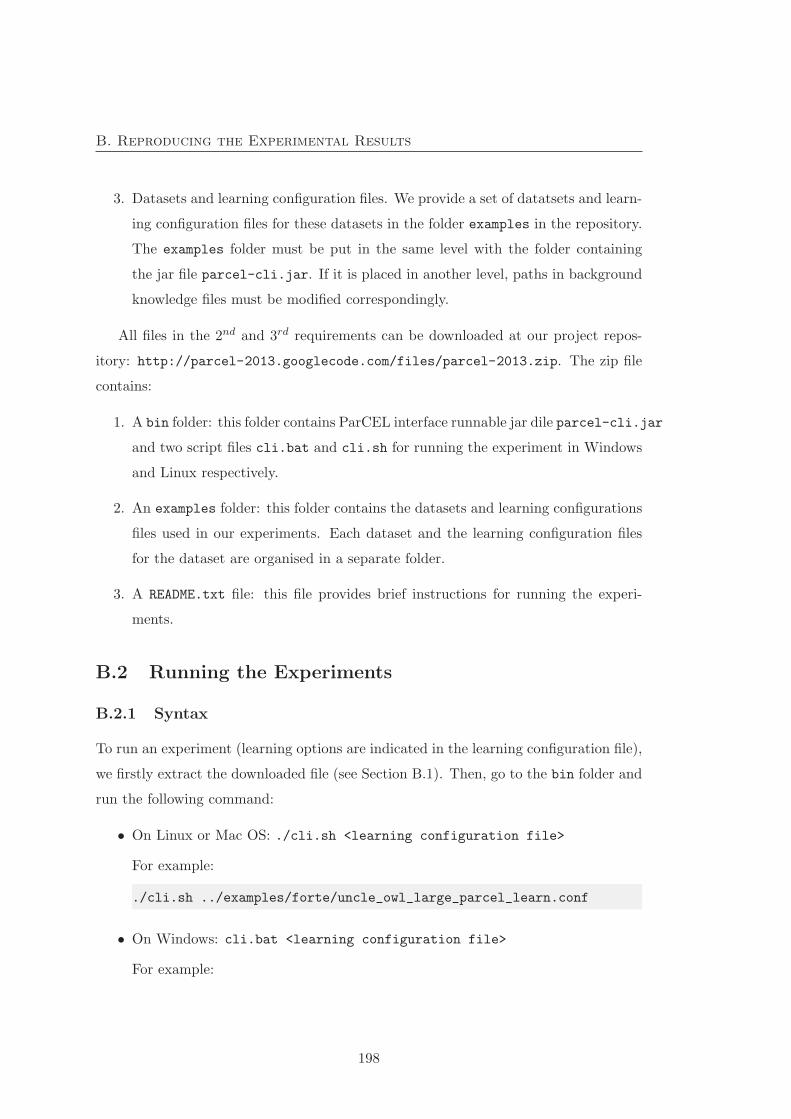
B. Reproducing the Experimental Results
3. Datasets and learning configuration files. We provide a set of datatsets and learn-
ing configuration files for these datasets in the folder examples in the repository.
The examples folder must be put in the same level with the folder containing
the jar file parcel-cli.jar. If it is placed in another level, paths in background
knowledge files must be modified correspondingly.
All files in the 2nd and 3rd requirements can be downloaded at our project repos-
itory: http://parcel-2013.googlecode.com/files/parcel-2013.zip. The zip file
contains:
1. A bin folder: this folder contains ParCEL interface runnable jar dile parcel-cli.jar
and two script files cli.bat and cli.sh for running the experiment in Windows
and Linux respectively.
2. An examples folder: this folder contains the datasets and learning configurations
files used in our experiments. Each dataset and the learning configuration files
for the dataset are organised in a separate folder.
3. A README.txt file: this file provides brief instructions for running the experi-
ments.
B.2 Running the Experiments
B.2.1 Syntax
To run an experiment (learning options are indicated in the learning configuration file),
we firstly extract the downloaded file (see Section B.1). Then, go to the bin folder and
run the following command:
• On Linux or Mac OS: ./cli.sh <learning configuration file>
For example:
./cli.sh ../examples/forte/uncle_owl_large_parcel_learn.conf
• On Windows: cli.bat <learning configuration file>
For example:
198

B. Reproducing the Experimental Results
cli.bat ..\examples\forte\uncle_owl_large_parcel_learn.conf
The learning result is outputted both to the terminal and a log file saved in the
bin\log folder.
B.2.2 Learning configuration file naming conventions
Learning configuration files are named using the following naming convention:
<dataset name>_<algorithm name>_<experiment type>.conf
Algorithm name can be: celoe, parcel or parcelex (SPaCEL). On the other
hand, experiment type is abbreviated as follows: learn stands for learning only, cross
stands for running cross-validation and fort stands for running cross-validation with
fortification.
For example, the file uncle owl large parcel learn.conf is a learning config-
uration file for learning the concept for uncle owl large dataset using the parcel
algorithm without running cross-validation procedure.
B.3 Learning Configuration
Our algorithms are developed based on the DL-Learner framework as described in Sec-
tion A.1.2. Therefore, a learning configuration file must provide sufficient information
for the four components. An example of a typical learning configuration file is:
//command line interface (CLI) component
cli.type = "org.dllearner.cli.ParCEL.CLI"
cli.performCrossValidation = true
cli.nrOfFolds = 3
cli.fortification = false
cli.fairComparison = false
//knowledge source component
ks.type = "OWL File"
199
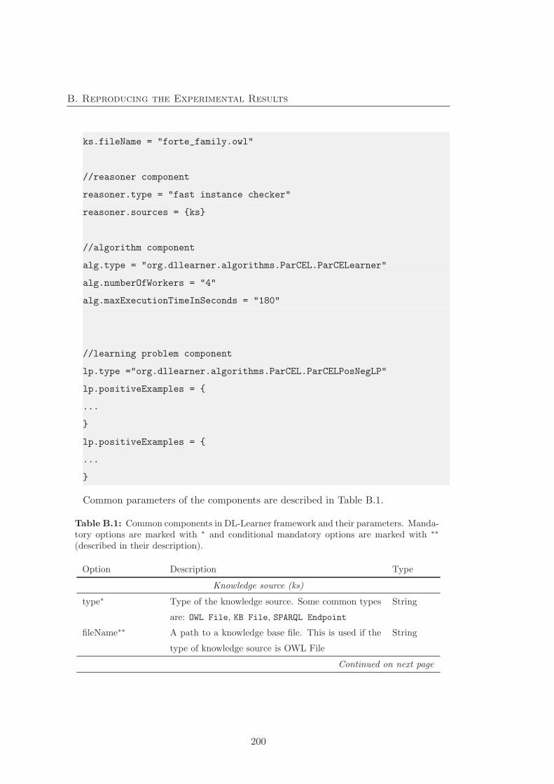
B. Reproducing the Experimental Results
ks.fileName = "forte_family.owl"
//reasoner component
reasoner.type = "fast instance checker"
reasoner.sources = {ks}
//algorithm component
alg.type = "org.dllearner.algorithms.ParCEL.ParCELearner"
alg.numberOfWorkers = "4"
alg.maxExecutionTimeInSeconds = "180"
//learning problem component
lp.type ="org.dllearner.algorithms.ParCEL.ParCELPosNegLP"
lp.positiveExamples = {
...
}
lp.positiveExamples = {
...
}
Common parameters of the components are described in Table B.1.
Table B.1: Common components in DL-Learner framework and their parameters. Manda-tory options are marked with ∗ and conditional mandatory options are marked with ∗∗
(described in their description).
Option Description Type
Knowledge source (ks)
type∗ Type of the knowledge source. Some common types
are: OWL File, KB File, SPARQL Endpoint
String
fileName∗∗ A path to a knowledge base file. This is used if the
type of knowledge source is OWL File
String
Continued on next page
200

B. Reproducing the Experimental Results
Table B.1 – continued
Option Description Type
url∗∗ A path to a KB file or an URL of a SPARQL End-
point. This is used if the knowledge source type is
KB File or SPARQL Endpoint.
String
Reasoner
type∗ Type of the reasoner. Some common reasoners
are: fast instance checker, PelletReasonser,
DIGReasoner.
String
source∗∗ A knowledge source component. This is used
if the reasoner is fast instance checker or
PelletReasoner.
Component
(ks)
url∗∗ An URL of a DIG reasoner. This is used if the rea-
soner is DIGReasoner.
String
Learning problem (lp)
type∗ Type of the learning problem. It can be
posNegStandard, ClassLearningProblem,
PosOnlyLP, ParCELPosNegLP (full qualified names
are recommended).
String
positiveExamples∗∗ Set of positive examples. Set of
string
negativeExamples∗∗ Set of negative examples. Set of
string
Learning algorithm (la)
type∗ Learning algorithm type. Common algorithms are:
celoe, ocel, ParCELearner, ParCELearnerExV2
(SPaCEL) (full qualified names are recommended).
String
maxExcution-
TimeInSeconds
Maximal seconds that an algorithm is allowed to
learn a given problem.
Integer
numberOfWorkers Maximal number of workers (see Chapter 5) are used
in learning. This is used with ParCEL and SPaCEL
algorithms.
Integers
noisePercentage Percentage of the negative examples are allowed to
be covered by a learnt concept.
Integer
Continued on next page
201
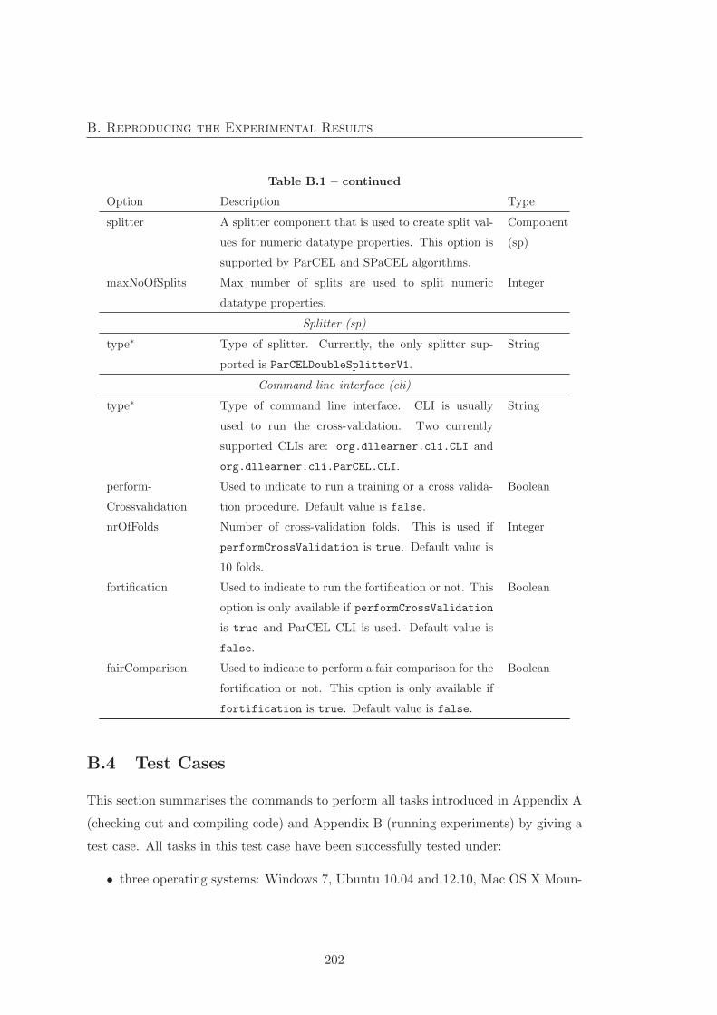
B. Reproducing the Experimental Results
Table B.1 – continued
Option Description Type
splitter A splitter component that is used to create split val-
ues for numeric datatype properties. This option is
supported by ParCEL and SPaCEL algorithms.
Component
(sp)
maxNoOfSplits Max number of splits are used to split numeric
datatype properties.
Integer
Splitter (sp)
type∗ Type of splitter. Currently, the only splitter sup-
ported is ParCELDoubleSplitterV1.
String
Command line interface (cli)
type∗ Type of command line interface. CLI is usually
used to run the cross-validation. Two currently
supported CLIs are: org.dllearner.cli.CLI and
org.dllearner.cli.ParCEL.CLI.
String
perform-
Crossvalidation
Used to indicate to run a training or a cross valida-
tion procedure. Default value is false.
Boolean
nrOfFolds Number of cross-validation folds. This is used if
performCrossValidation is true. Default value is
10 folds.
Integer
fortification Used to indicate to run the fortification or not. This
option is only available if performCrossValidation
is true and ParCEL CLI is used. Default value is
false.
Boolean
fairComparison Used to indicate to perform a fair comparison for the
fortification or not. This option is only available if
fortification is true. Default value is false.
Boolean
B.4 Test Cases
This section summarises the commands to perform all tasks introduced in Appendix A
(checking out and compiling code) and Appendix B (running experiments) by giving a
test case. All tasks in this test case have been successfully tested under:
• three operating systems: Windows 7, Ubuntu 10.04 and 12.10, Mac OS X Moun-
202
B. Reproducing the Experimental Results
tain Lion, and
• JDK 1.6.x and 1.7.x.
In this section, we show the test case under Ubuntu 12.10 and JDK 1.7.0 09. The
only difference when running this test case under other operating systems is the in-
stallation of the required softwares. In Ubuntu, we use apt-get utility for installing
required softwares while in Windows and Mac OS, we can use installers available on
their vendor’s website. Otherwise, the commands for the remaining steps are similar
to in Ubuntu. Following is the summary of this test case:
• Objectives: are to successfully:
1. check out and compile the project code of this thesis, and
2. run three learning algorithms CELOE, ParCEL and SPaCEL for the forte-uncle
dataset.
• Pre-conditions:
1. A fresh Ubuntu system (i.e. system has not been installed any required
softwares described in A.2) with an internet connection.
2. The project code is committed to the repository at https://code.google.
com/p/parcel-2013/.
3. Maven3 had been downloaded from http://maven.apache.org/.
The test case execution (actions and results) is demonstrated by showing the figures
that are captured from the execution. Summary of actions and expected results are
given in Table B.2.
203
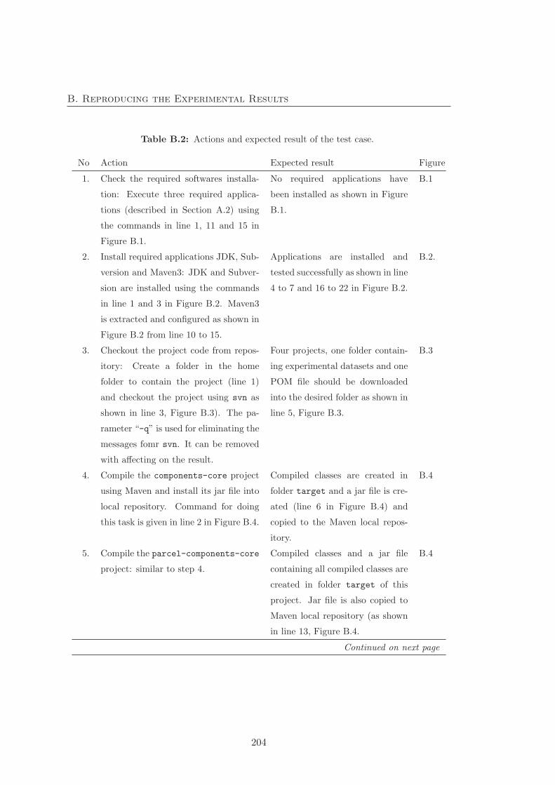
B. Reproducing the Experimental Results
Table B.2: Actions and expected result of the test case.
No Action Expected result Figure
1. Check the required softwares installa-
tion: Execute three required applica-
tions (described in Section A.2) using
the commands in line 1, 11 and 15 in
Figure B.1.
No required applications have
been installed as shown in Figure
B.1.
B.1
2. Install required applications JDK, Sub-
version and Maven3: JDK and Subver-
sion are installed using the commands
in line 1 and 3 in Figure B.2. Maven3
is extracted and configured as shown in
Figure B.2 from line 10 to 15.
Applications are installed and
tested successfully as shown in line
4 to 7 and 16 to 22 in Figure B.2.
B.2.
3. Checkout the project code from repos-
itory: Create a folder in the home
folder to contain the project (line 1)
and checkout the project using svn as
shown in line 3, Figure B.3). The pa-
rameter “-q” is used for eliminating the
messages fomr svn. It can be removed
with affecting on the result.
Four projects, one folder contain-
ing experimental datasets and one
POM file should be downloaded
into the desired folder as shown in
line 5, Figure B.3.
B.3
4. Compile the components-core project
using Maven and install its jar file into
local repository. Command for doing
this task is given in line 2 in Figure B.4.
Compiled classes are created in
folder target and a jar file is cre-
ated (line 6 in Figure B.4) and
copied to the Maven local repos-
itory.
B.4
5. Compile the parcel-components-core
project: similar to step 4.
Compiled classes and a jar file
containing all compiled classes are
created in folder target of this
project. Jar file is also copied to
Maven local repository (as shown
in line 13, Figure B.4.
B.4
Continued on next page
204
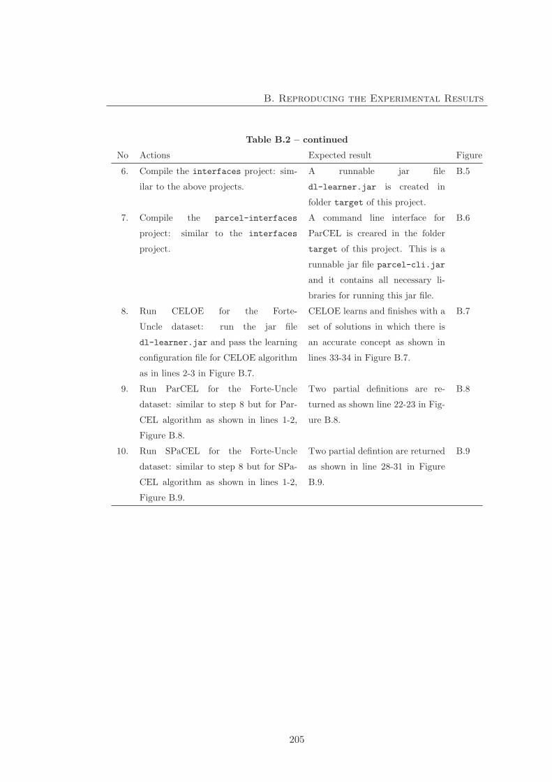
B. Reproducing the Experimental Results
Table B.2 – continued
No Actions Expected result Figure
6. Compile the interfaces project: sim-
ilar to the above projects.
A runnable jar file
dl-learner.jar is created in
folder target of this project.
B.5
7. Compile the parcel-interfaces
project: similar to the interfaces
project.
A command line interface for
ParCEL is creared in the folder
target of this project. This is a
runnable jar file parcel-cli.jar
and it contains all necessary li-
braries for running this jar file.
B.6
8. Run CELOE for the Forte-
Uncle dataset: run the jar file
dl-learner.jar and pass the learning
configuration file for CELOE algorithm
as in lines 2-3 in Figure B.7.
CELOE learns and finishes with a
set of solutions in which there is
an accurate concept as shown in
lines 33-34 in Figure B.7.
B.7
9. Run ParCEL for the Forte-Uncle
dataset: similar to step 8 but for Par-
CEL algorithm as shown in lines 1-2,
Figure B.8.
Two partial definitions are re-
turned as shown line 22-23 in Fig-
ure B.8.
B.8
10. Run SPaCEL for the Forte-Uncle
dataset: similar to step 8 but for SPa-
CEL algorithm as shown in lines 1-2,
Figure B.9.
Two partial defintion are returned
as shown in line 28-31 in Figure
B.9.
B.9
205

B. Reproducing the Experimental Results
Figure B.1: Check required softwares in the system including JDK, Subversion andMaven.
Figure B.2: Install required softwares: JDK, Subversion and Maven. JDK and Subversionare installed using apt-get while Maven3 is installed manually. “> null” in lines 1, 3 and11 is used to turn off the messages when install or extract the softwares.
206

B. Reproducing the Experimental Results
Figure B.3: Check out the project from the repository. “-q” in line 3 is used to tell svnnot to display the messages.
Figure B.4: Compile the DL-Leaner and ParCEL core components project.
Figure B.5: Compile the interface project.
Figure B.6: Compile the ParCEL CLI project.
207
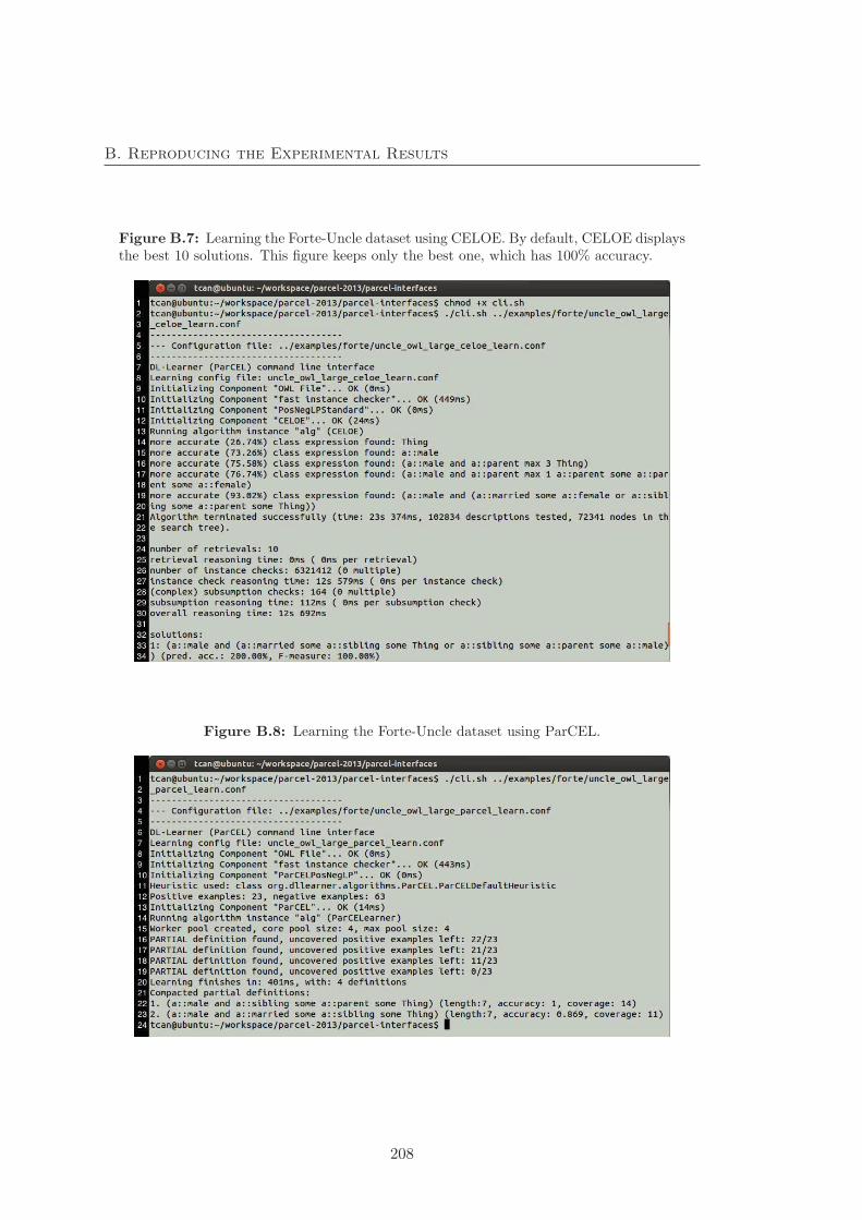
B. Reproducing the Experimental Results
Figure B.7: Learning the Forte-Uncle dataset using CELOE. By default, CELOE displaysthe best 10 solutions. This figure keeps only the best one, which has 100% accuracy.
Figure B.8: Learning the Forte-Uncle dataset using ParCEL.
208
B. Reproducing the Experimental Results
Figure B.9: Learning the Forte-Uncle dataset using SPaCEL.
209

B. Reproducing the Experimental Results
210
Appendix C
List of Publications
Parts of this thesis are based on previously published materials as follows:
• An C. Tran, Jens Dietrich, Hans W. Guesgen, and Stephen Mars-
land. Improving Predictive Specificity of Description Logic Learner
by Fortification. Journal of Machine Learning Research - Proceedings Track,
29:419-434, 2013.
• An C. Tran, Jens Dietrich, Hans W. Guesgen, and Stephen Marsland.
An Approach to Numeric Refinement in Description Logic Learning
for Learning Activities Duration in Smart Homes. In Proceeding of the
Twenty-Seventh AAAI Conference on Artificial Intelligence (AAAI-13) Work-
shop on Space, Time and Ambient Intelligence, pages 22–28, 2013.
• An C. Tran, Jens Dietrich, Hans W. Guesgen, and Stephen Marsland.
Two-way Parallel Class Expression Learning. Journal of Machine Learning
Research - Proceedings Track, 25:443–458, 2012.
• An C. Tran, Jens Dietrich, Hans W. Guesgen, and Stephen Marsland.
An approach to parallel class expression learning. In Rules on the Web:
Research and Applications, pages 302–316. Springer, 2012.
• An C. Tran, Stephen Marsland, Jens Dietrich, Hans W. Guesgen,
and Paul Lyons. Use cases for abnormal behaviour detection in smart
211

C. List of Publications
homes. In Aging Friendly Technology for Health and Independence, pages 144–
151. Springer, 2010.
• Paul Lyons,, An C. Tran, Joe H. Steinhauer, Stephen Marsland,
Jens Dietrich, and Hans W. Guesgen. Exploring the responsibilities
of single-inhabitant Smart Homes with Use Cases. Journal of Ambient
Intelligence and Smart Environments, 2(3):211–232, 2010.
212

Glossary
AL a short for Attribute Language, the most basic language in the description logic
language family. 14
SRIOQ a description logic language, which is an underlying logic for the most-up-to-
date W3C recommendation for semantic web language OWL2-DL. 14, 15
BOTTOM a special concept in description logics (also denoted by ⊥) with no individuals
are its instances. 15, 18
TOP a special concept in description logics (also denoted by ) that subsumes all other
concepts in the TBox, i.e. all individuals in the knowledge base are its instances.
15, 18, 24
Thing the super class of all class in a OWL knowledge base (ontology). 24
SPaCEL a short for Symmetric Class Expression Learning algorithm (see Chapter 6).
106
ParCEL a short for Parallel Class Expression Learning algorithm (see Chapter 5). 62,
68, 79
ABox a part description logic knowledge base that contains concept and role asser-
tions. 17, 20
axiom (in DLs) an axiom is a concept in the form of C D (inclusion axiom) or
C ≡ D (equality axiom), where C and D are concepts. 19, 26
213
Glossary
CELOE a short for Class Expression Learner for Ontology Engineering algorithm.
This is an OWL learning algorithm in DL-Learner framework developed by Lehmann
et al. [80]. 33, 49, 62, 68
CPU time the actual time taken by the CPU(s) to process a certain task. 41
decidable in general, a logical system is decidable if it can compute the truth value
of all inference tasks within a finite time. In description logics, a description
logic language is decidable if there exist algorithms that can give an answer for a
subsumption (or satisfiability) check in a finite number of steps. 13, 15, 24
DL a short for Description Logics, a family of knowledge representation formalisms.
1, 13
ILP a symbolic approach in machine learning (i.e. an intersection of Machine Learning
and Logic Programming), which aims to learn general rules from specific facts. 1
OCEL a short for Ontology Class Expression Learning Algorithm. This is an OWL
learning algorithm in DL-Learner framework developed by Lehmann et al. [80].
33, 49, 63
OWL a short for Web Ontology Language which is a family of knowledge representa-
tion languages for the Semantic Web endorsed by World Wide Web Consortium
(W3C). 3, 23
RBox a part of description logic knowledge base that contains role axioms. 17
scalable (a system) is able to handle a growing amount of work in a capable manner
or to enlarge to accommodate that growth [20]. 34
semi-decidable in general, a logical system is semi-decidable if it can compute the
truth value of all inference tasks within a finite time if the inference is hold but
it may not give the answer if the inference is not hold. In description logics,
a description logic language is semi-decidable if there exist algorithms that can
give an answer for a subsumption (or satisfiability) check in a finite number of
214

Glossary
steps if the subsumption (or satisfiability) is hold and there may not have such
an algorithm if the subsumption (or satisfiability) is not hold. 24
speeding up in parallel computing, speed-up aims to decrease the time taken for
performing a task in proportion to the increase of the degree of parallelisation. 4
TBox a part of description logic knowledge base that contains concept and role axioms.
In case that the knowledge base has RBox, this part contains only concept axioms.
17, 19
wall-clock time the actual time taken by a computer to process a task that includes
the CPU time, I/O time and delay time caused by waiting for availability of
required resources. 41
215

Glossary
216
References
[1] Michael Armbrust, Armando Fox, Rean Griffith, Anthony D. Joseph,
Randy Katz, Andy Konwinski, Gunho Lee, David Patterson, Ariel
Rabkin, Ion Stoica, et al. A view of cloud computing. Communications
of the ACM, 53(4):50–58, 2010.
[2] Franz Baader. The Instance Problem and the Most Specific Concept
in the Description Logic EL w.r.t Terminological Cycles with Descrip-
tive Semantics. In KI 2003: Advances in Artificial Intelligence, pages 64–78.
Springer, 2003.
[3] Franz Baader, Diego Calvanese, Deborah L. McGuinness, Daniele
Nardi, and Peter F. Patel-Schneider. The description logic handbook:
Theory, implementation and applications. Cambridge University Press, 2010.
[4] Franz Baader, Ian Horrocks, and Ulrike Sattler. Description logics
as ontology languages for the Semantic Web. Mechanizing Mathematical
Reasoning, pages 228–248, 2005.
[5] Franz Baader, Ralf Kusters, and Ralf Molitor. Computing least
common subsumers in Description logics with existential restrictions.
In International Joint Conference on Artificial Intelligence, pages 96–101. Morgan
Kaufmann Publishers Inc., 1999.
[6] Liviu Badea and Shan-Hwei Nienhuys-Cheng. A refinement operator
for Description logics. Inductive Logic Programming, pages 40–59, 2000.
217
REFERENCES
[7] Dennis Bahler. The Induction of rules for predicting chemical Car-
cinogenesis in Rodents. In Intelligent Systems for Molecular Biology, pages
29–37. AAAI/MIT Press, 1993.
[8] Jonathan Barnes. Aristotle’s Posterior analytics. Oxford University Press,
1976.
[9] Jonathan Barnes. Posterior analytics. Oxford University Press, USA, 1994.
[10] Sean Bechhofer, Ralf Moller, and Peter Crowther. The DIG De-
scription logic interface: DIG/1.1. In Proceedings of the 2003 Description
Logic Workshop (DL 2003), 2003.
[11] Sean Bechhofer, Raphael Volz, and Phillip Lord. Cooking the Se-
mantic Web with the OWL API. The Semantic Web-ISWC 2003, pages
659–675, 2003.
[12] Dave Beckett and Brian McBride. RDF/XML Syntax specification
(revised). W3C Recommendation, 2004.
[13] David Beckett. New syntaxes for RDF. Technical report, Institute For
Learning And Research Technology, Bristol, 2004.
[14] Tim Berners-Lee, James Hendler, Ora Lassila, et al. The Semantic
Web. Scientific American, 284(5):28–37, 2001.
[15] Milind Bhandarkar. MapReduce programming with apache Hadoop.
In Parallel & Distributed Processing (IPDPS) Symposium, pages 1–1. IEEE, 2010.
[16] Chris Biemann. Ontology learning from text: A survey of methods. In
LDV forum, number 2, pages 75–93. 2005.
[17] Christian Bizer, Tom Heath, and Tim Berners-Lee. Linked data - The
story so far. International Journal on Semantic Web and Information Systems
(IJSWIS), 5(3):1–22, 2009.
218

REFERENCES
[18] Christian Bizer, Jens Lehmann, Georgi Kobilarov, Soren Auer,
Christian Becker, Richard Cyganiak, and Sebastian Hellmann. DB-
pedia – A crystallization point for the Web of data. Web Semantics:
Science, Services and Agents on the World Wide Web, 7(3):154–165, 2009.
[19] James P. Bliss. The Cry Wolf Phenomenon and its Effects on Alarm Responses
(False Alarms). PhD thesis, PhD dissertation, University of Central Florida,
USA, 1993.
[20] Andre B. Bondi. Characteristics of scalability and their impact on
performance. In Proceedings of the 2nd International workshop on Software
and Performance, WOSP ’00, pages 195–203, New York, NY, USA, 2000. ACM.
[21] Ronald J. Brachman. Structured inheritance networks. Research in
Natural Language Understanding, Quarterly Progress Report, (1):36–78, 1978.
[22] Shlomo Breznitz. Cry wolf: The psychology of false alarms. Lawrence Erlbaum
Associates Hillsdale, NJ, 1984.
[23] HAYES Brian, Thomas Brunschwiler, Heinz Dill, Hanspeter Christ,
Babak Falsafi, Markus Fischer, Stella Gatziu Grivas, Claudio Gio-
vanoli, Roger Eric Gisi, Reto Gutmann, et al. Cloud computing.
Communications of the ACM, 51(7):9–11, 2008.
[24] Stephane Campinas, Diego Ceccarelli, Thomas E . Perry, Renaud
Delbru, Krisztian Balog, and Giovanni Tummarello. The Sindice-
2011 dataset for entity-oriented search in the web of data. In 1st Inter-
national Workshop on Entity-Oriented Search (EOS), pages 26–32, 2011.
[25] Thomas W. Christopher and George Thiruvathukal. High Performance
Java Computing: Multi-threaded and Networked programming. Prentice Hall,
2000.
[26] Cheng Chu, Sang Kyun Kim, Yi-An Lin, YuanYuan Yu, Gary Brad-
ski, Andrew Y Ng, and Kunle Olukotun. Map-Reduce for machine
219

REFERENCES
learning on multicore. Advances in neural information processing systems,
19:281–288, 2007.
[27] Keith L. Clark. Negation As Failure. In Logic and Data Bases, pages
293–322. Springer, 1978.
[28] Keith L. Clark. Parallel logic programming. The Computer Journal,
33(6):482–493, 1990.
[29] Kendall Grant Clark, Lee Feigenbaum, and Elias Torres. SPARQL
protocol for RDF. World Wide Web Consortium (W3C) Recommendation,
2008.
[30] William W Cohen, Alex Borgida, and Haym Hirsh. Computing least
common subsumers in Description logics. In Proceedings of the National
Conference on Artificial Intelligence, pages 754–754. John Wiley & Sons Ltd.,
1992.
[31] William W. Cohen and Haym Hirsh. Learnability of Description logics.
In Proceedings of the fifth annual workshop on Computational learning theory,
pages 116–127. ACM, 1992.
[32] William W. Cohen and Haym Hirsh. Learning the CLASSIC descrip-
tion logic: Theoretical and experimental results. In Proceedings of the 4th
International conference on Principles of Knowledge representation and Reason-
ing, pages 121–133, 1994.
[33] Claudia d’Amato, Nicola Fanizzi, and Floriana Esposito. A dissimi-
larity measure for ALC concept descriptions. In Proceedings of the 2006
ACM Symposium on Applied Computing, pages 1695–1699. ACM, 2006.
[34] Claudia d’Amato, Nicola Fanizzi, and Floriana Esposito. A semantic
similarity measure for expressive Description logics. In Proceedings of
Convegno Italiano di Logica Computazionale, CILC05, 2009.
[35] John Davies, Rudi Studer, and Paul Warren. Semantic Web technologies:
Trends and research in ontology-based systems. Wiley, 2006.
220
REFERENCES
[36] Jeffrey Dean and Sanjay Ghemawat. MapReduce: Simplified data
processing on large clusters. Communications of the ACM, 51(1):107–113,
2008.
[37] Luc Dehaspe and Luc De Raedt. Parallel inductive logic programming.
In Proceedings of the MLnet Familiarization Workshop on Statistics, Machine
Learning and Knowledge Discovery in Databases, page 5, 1995.
[38] Kathrin Dentler, Ronald Cornet, Annette ten Teije, and Nicolette
de Keizer. Comparison of reasoners for large ontologies in the OWL2
EL profile. Semantic Web, 2(2):71–87, 2011.
[39] Felix Distel. Model-Based Most Specific Concepts in Some Inexpres-
sive Description Logics. CEUR Workshop Proceeding, 2010.
[40] Francesco M Donini, Daniele Nardi, and Riccardo Rosati. Descrip-
tion logics of minimal knowledge and Negation As Failure. ACM Trans-
actions on Computational Logic (TOCL), 3(2):177–225, 2002.
[41] Jaliya Ekanayake and Geoffrey Fox. High performance parallel com-
puting with clouds and cloud technologies. In Cloud Computing, pages
20–38. Springer, 2010.
[42] Jaliya Ekanayake, Shrideep Pallickara, and Geoffrey Fox. MapRe-
duce for data intensive scientific analyses. In Proceeding of the 2008 Fourth
IEEE International Conference on eScience, pages 277–284. IEEE, 2008.
[43] Floriana Esposito, Nicola Fanizzi, Luigi Iannone, Ignazio Palmisano,
and Giovanni Semeraro. Knowledge-intensive induction of terminolo-
gies from metadata. The Semantic Web–ISWC 2004, pages 441–455, 2004.
[44] Nicola Fanizzi and Claudia d’Amato. A similarity measure for the
ALN Description logic. In Proceedings of the Italian Conference on Compu-
tational Logic (CILC), pages 26–27, 2006.
221
REFERENCES
[45] Nicola Fanizzi, Claudia d’Amato, and Floriana Esposito. DL-FOIL
concept learning in Description logics. Inductive Logic Programming, pages
107–121, 2008.
[46] Usama Fayyad and Keki Irani. Multi-interval discretization of
continuous-valued attributes for classification learning. In The 13th In-
ternational Joint Conference on Artificial Intelligence, pages 1022–1027, 1993.
[47] Pascal Felber and Michael K. Reiter. Advanced concurrency control
in Java. Concurrency and Computation: Practice and Experience, 14(4):261–
285, 2002.
[48] Dieter Fensel, Frank van Harmelen, Bosse Andersson, Paul Bren-
nan, Hamish Cunningham, Emanuele Della Valle, Florian Fischer,
Zhisheng Huang, Atanas Kiryakov, TK-I Lee, et al. Towards LarKC:
A platform for web-scale reasoning. In Semantic Computing, 2008 IEEE
International Conference on, pages 524–529. IEEE, 2008.
[49] Nuno A. Fonseca, Ashwin Srinivasan, Fernando Silva, and Rui Ca-
macho. Parallel ILP for distributed-memory architectures. Machine
learning, 74(3):257–279, 2009.
[50] Andrew Frank and Arthur Asuncion. UCI Machine learning reposi-
tory, 2010. Available from: http://archive.ics.uci.edu/ml.
[51] Dov M. Gabbay, Christopher John Hogger, John Alan Robinson,
J. Siekmann, Donald Nute, and Anthony Galton. Handbook of Logic
in Artificial Intelligence and Logic Programming. Clarendon Press, 1998.
[52] Anne Geffre, Kristen Friedrichs, Kendal Harr, Didier Concordet,
Catherine Trumel, and Jean-Pierre Braun. Reference values: A re-
view. Veterinary Clinical Pathology, 38(3):288–298, 2009.
[53] Steve Gregory. Parallel logic programming in PARLOG: The language and
its implementation. Addison-Wesley Pub. Co. Inc., Reading, MA, 1987.
222
REFERENCES
[54] Pierre Grenon, Barry Smith, and Louis J. Goldberg. Biodynamic on-
tology: Applying BFO in the Biomedical domain. Ontologies in Medicine,
102:20, 2004.
[55] Volker Haarslev, Kay Hidde, Ralf Moller, and Michael Wessel. The
RacerPro knowledge representation and reasoning system. Semantic
Web, 3(3):267–277, 2012.
[56] Volker Haarslev and Ralf Moller. Racer: An OWL Reasoning agent
for the Semantic Web. In Proc. of the International Workshop on Applications,
Products and Services of Web-based Support Systems, in conjunction with, pages
91–95, 2003.
[57] Sebastian Hellmann. Comparison of Concept learning algorithms. Master’s
thesis, The University of Leipzig, 2008.
[58] Sebastian Hellmann, Jens Lehmann, and Soren Auer. Learning of
OWL class descriptions on very large knowledge bases. International
Journal on Semantic Web and Information Systems (IJSWIS), 5(2):25–48, 2009.
[59] Pascal Hitzler, Markus Krotzsch, Bijan Parsia, Peter F. Patel-
Schneider, and Sebastian Rudolph. OWL 2 Web ontology language
primer. W3C Recommendation, 27:1–123, 2009.
[60] Pascal Hitzler, Markus Krotzsch, and Sebastian Rudolph. Founda-
tions of semantic web technologies. Chapman and Hall/CRC, 2009.
[61] Matthew Horridge et al. A Practical Guide To Building OWL On-
tologies Using Protege 4 and CO-ODE Tools Edition 1.2. The University
of Manchester, 2009.
[62] Matthew Horridge and Peter F. Patel-Schneider. OWL 2 web on-
tology language Manchester syntax. W3C Working Group Note, 2009.
[63] Ian Horrocks. FaCT and iFaCT. In Proceedings of the International Work-
shop on Description Logics (DL99), pages 133–135, 1999.
223
REFERENCES
[64] Ian Horrocks, Oliver Kutz, and Ulrike Sattler. The even more irre-
sistible SROIQ. In Proceeding of the 10th International Conference on Princi-
ples of Knowledge Representation and Reasoning (KR 2006), pages 57–67, 2006.
[65] Ian Horrocks and Peter F. Patel-Schneider. Optimizing description
logic subsumption. Journal of Logic and Computation, 9(3):267–293, 1999.
[66] Luigi Iannone, Ignazio Palmisano, and Nicola Fanizzi. An algorithm
based on counterfactuals for concept learning in the Semantic Web.
Applied Intelligence, 26(2):139–159, 2007.
[67] Paul Jaccard. Etude comparative de la distribution florale dans une portion
des Alpes et du Jura. Impr. Corbaz, 1901.
[68] Krzysztof Janowicz. Sim-DL: Towards a Semantic Similarity Mea-
surement Theory for the Description Logic ALCNR in Geographic
Information Retrieval. In On the Move to Meaningful Internet Systems 2006:
OTM 2006 Workshops, pages 1681–1692. Springer, 2006.
[69] Frederik Janssen and Johannes Furnkranz. On trading off consistency
and coverage in inductive rule learning. In Proceedings of the LWA, pages
306–313. Citeseer, 2006.
[70] Frederik Janssen and Johannes Furnkranz. An empirical investiga-
tion of the trade-off between consistency and coverage in rule learning
heuristics. In Discovery Science, pages 40–51. Springer, 2008.
[71] Aditya Kalyanpur, Bijan Parsia, Matthew Horridge, and Evren
Sirin. Finding all justifications of OWL DL entailments. The Seman-
tic Web, pages 267–280, 2007.
[72] Jorg-Uwe Kietz and Katharina Morik. A polynomial approach to
the constructive induction of structural knowledge. Machine Learning,
14(2):193–217, 1994.
[73] Lauwerens Kuipers and Harald Niederreiter. Uniform distribution of
sequences. Courier Dover Publications, 2006.
224
REFERENCES
[74] Ralf Kusters and Ralf Molitor. Computing most specific concepts
in Description logics with existential restrictions. In LTCS-report 00-05,
Lufg Theoretical Computer Science, RWTH, 2000.
[75] Ralf Kusters and Ralf Molitor. Approximating most specific con-
cepts in Description logics with existential restrictions. AI Communica-
tions, 15(1):47–59, 2002.
[76] Nada Lavrac and Saso Dzeroski. Inductive logic programming: Techniques
and applications. New York, Ellis Horwood, 1994.
[77] Nada Lavrac and Luc De Raedt. Inductive logic programming: A
survey of European research. AI Communications, 8(1):3–19, 1995.
[78] Jens Lehmann. Hybrid learning of ontology classes. Machine Learning
and Data Mining in Pattern Recognition, pages 883–898, 2007.
[79] Jens Lehmann. DL-Learner: Learning concepts in Description logics.
The Journal of Machine Learning Research, 10:2639–2642, 2009.
[80] Jens Lehmann. Learning OWL Class Expressions. AKA Akademische Verlage-
sellschaft, 2010.
[81] Jens Lehmann, Soren Auer, Lorenz Buhmann, and Sebastian Tramp.
Class expression learning for ontology engineering. Web Semantics: Sci-
ence, Services and Agents on the World Wide Web, 9(1):71–81, 2011.
[82] Jens Lehmann and Pascal Hitzler. Concept learning in Description
logics using Refinement operators. Machine Learning, 78(1):203–250, 2010.
[83] Man Li, Xiaoyong Du, and Shan Wang. A semi-automatic ontology ac-
quisition method for the Semantic Web. Advances in Web-Age Information
Management, pages 209–220, 2005.
[84] Thorsten Liebig and Felix Muller. Parallelizing tableaux-based de-
scription logic reasoning. In On the Move to Meaningful Internet Systems
2007: OTM 2007 Workshops, pages 1135–1144. Springer, 2007.
225

REFERENCES
[85] Francesca A. Lisi and Donato Malerba. Ideal refinement of Descrip-
tions in AL-Log. Inductive Logic Programming, pages 215–232, 2003.
[86] John Wylie Lloyd. Foundations of logic programming. Springer-verlag Berlin,
1984.
[87] Yann Loyer and Umberto Straccia. Any-world assumptions in Logic
Programming. Theoretical Computer Science, 342(2):351–381, 2005.
[88] Paul Lyons, An C. Tran, H. Joe Steinhauer, Stephen Marsland, Jens
Dietrich, and Hans W. Guesgen. Exploring the responsibilities of
single-inhabitant Smart Homes with Use Cases. Journal of Ambient In-
telligence and Smart Environments, 2(3):211–232, 2010.
[89] Alexander Maedche and Steffen Staab. Mining ontologies from text.
Knowledge Engineering and Knowledge Management Methods, Models, and Tools,
pages 169–189, 2000.
[90] Alexander Maedche and Steffen Staab. Ontology learning for the
Semantic Web. IEEE Intelligent Systems, 16(2):72–79, 2001.
[91] Frank Manola, Eric Miller, and Brian McBride. RDF Primer. W3C
Recommendation, 10:1–107, 2004.
[92] Vincent Massol and Timothy M O’Brien. Maven: A developer’s notebook.
O’Reilly Media, Incorporated, 2005.
[93] Tohgoroh Matsui, Nobuhiro Inuzuka, Hirohisa Seki, and Hidenori
Itoh. Comparison of three parallel implementations of an induction
algorithm. In 8th Int. Parallel Computing Workshop, pages 181–188, 1998.
[94] Cynthia Matuszek, John Cabral, Michael Witbrock, and John DeO-
liveira. An introduction to the syntax and content of CYC. In Pro-
ceedings of the 2006 AAAI Spring Symposium on Formalizing and Compiling
Background Knowledge and Its Applications to Knowledge Representation and
Question Answering, 2006.
226
REFERENCES
[95] Brian McBride et al. The resource description framework (RDF) and
its vocabulary description language RDFS. Handbook on Ontologies, pages
51–66, 2004.
[96] Deborah L. McGuinness, Frank Van Harmelen, et al. OWL web on-
tology language overview. W3C Recommendation, 10(2004-03):10, 2004.
[97] Michael Mealling and Ray Denenberg. Report from the Joint
W3C/IETF URI Planning Interest Group: Uniform Resource Iden-
tifiers (URIs), URLs, and Uniform Resource Names (URNs): Clarifi-
cations and Recommendations. Technical report, RFC 3305, 2002.
[98] Marvin Minksy. A framework for representing knowledge. The Psychol-
ogy of Computer Vision, McGraw-Hill, pages 211–277, 1975.
[99] Tom M. Mitchell. Generalization as search. Artificial intelligence,
18(2):203–226, 1982.
[100] Boris Motik, Bernardo Cuenca Grau, Ian Horrocks, Zhe Wu, Achille
Fokoue, and Carsten Lutz. OWL 2 web ontology language: Profiles.
W3C Recommendation, 27:61, 2009.
[101] Stephen Muggleton. Inductive logic programming. New generation com-
puting, 8(4):295–318, 1991.
[102] Stephen Muggleton and Luc De Raedt. Inductive logic programming:
Theory and methods. The Journal of Logic Programming, 19:629–679, 1994.
[103] Todd Neideen and Karen Brasel. Understanding statistical tests. Jour-
nal of surgical education, 64(2):93–96, 2007.
[104] Shan-Hwei Nienhuys-Cheng and Ronald De Wolf. Foundations of Induc-
tive logic programming. Springer, 1997.
[105] Ian Niles and Adam Pease. Towards a standard upper ontology. In
Proceedings of the International Conference on Formal Ontology in Information
Systems, pages 2–9. ACM, 2001.
227
REFERENCES
[106] Hayato Ohwada and Fumio Mizoguchi. Parallel execution for speeding
up inductive logic programming systems. In Discovery Science, pages 75–
75. Springer, 1999.
[107] Bijan Parsia and Evren Sirin. Pellet: An OWL DL reasoner. In Third
International Semantic Web Conference-Poster, page 18, 2004.
[108] J. Ross Quinlan. Learning logical definitions from relations. Machine
learning, 5(3):239–266, 1990.
[109] M. Ross Quinlan. Semantic memory. Semantic Information Processing,
pages 216–270, 1968.
[110] Anand Rajaraman and Jeffrey David Ullman. Mining of massive datasets.
Cambridge University Press, 2011.
[111] Michael Ratcliffe and Jean-Claude Syre. A parallel logic program-
ming language for PEPSys. In Proceedings of the 10th International Joint
Conference on Artificial Intelligence, 1, pages 48–55. Morgan Kaufmann Pub-
lishers Inc., 1987.
[112] Lawrence Reeve and Hyoil Han. Survey of Semantic annotation plat-
forms. In Symposium on Applied Computing: Proceedings of the 2005 ACM
Symposium on Applied Computing, pages 1634–1638, 2005.
[113] Bradley L. Richards and Raymond J. Mooney. Automated refinement
of first-order Horn-clause domain theories. Machine Learning, 19(2):95–
131, 1995.
[114] Riccardo Rosati. DL+ Log: Tight integration of Description logics and
Disjunctive datalog. Proceeding of the 10th International Conference on the
Principles of Knowledge Representation and Reasoning (KR 2006), pages 68–78,
2006.
[115] Celine Rouveirol and Veronique Ventos. Towards learning in
CARIN-ALN. Inductive Logic Programming, pages 191–208, 2000.
228
REFERENCES
[116] Julian Seidenberg and Alan Rector. Web ontology segmentation:
Analysis, classification and use. In Proceedings of the 15th International
Conference on World Wide Web, pages 13–22. ACM, 2006.
[117] Rob Shearer, Boris Motik, and Ian Horrocks. HermiT: A highly-
efficient OWL reasoner. In Proceedings of the 5th International Workshop on
OWL: Experiences and Directions (OWLED 2008), pages 26–27, 2008.
[118] Raymond M. Smullyan. First-order logic. Dover Publications, 1995.
[119] Vaclav Snasel, Pavel Moravec, and Jaroslav Pokorny. WordNet
ontology based model for web retrieval. In Proceedings in the Interna-
tional Workshop on Challenges in Web Information Retrieval and Integration
(WIRI’05), pages 220–225. IEEE, 2005.
[120] Antonio A. Snchez-Ruiz, Santiago Ontan, PedroAntonio Gonzlez-
Calero, and Enric Plaza. Measuring Similarity in Description Logics
Using Refinement Operators. In Ashwin Ram and Nirmalie Wiratunga,
editors, Case-Based Reasoning Research and Development, 6880 of Lecture Notes
in Computer Science, pages 289–303. Springer Berlin Heidelberg, 2011.
[121] Marina Sokolova, Nathalie Japkowicz, and Stan Szpakowicz. Beyond
accuracy, F-score and ROC: A family of discriminant measures for
performance evaluation. AI 2006: Advances in Artificial Intelligence, pages
1015–1021, 2006.
[122] Ramakrishna Soma and Viktor K. Prasanna. Parallel inferencing for
OWL knowledge bases. In 37th International Conference on Parallel Process-
ing (ICPP’08), pages 75–82. IEEE, 2008.
[123] Ashwin Srinivasan. The Aleph Manual, 2004. Available from: http://www.
comlab.ox.ac.uk/oucl/research/areas/machlearn/Aleph/.
[124] Ashwin Srinivasan, Ross D. King, Stephen Muggleton, and
Michael JE. Sternberg. Carcinogenesis predictions using ILP. Inductive
Logic Programming, pages 273–287, 1997.
229

REFERENCES
[125] Steffen Staab and Rudi Studer. Handbook on Ontologies. Springer Verlag,
2009.
[126] Vaidy S. Sunderam. PVM: A framework for parallel distributed com-
puting. Concurrency: practice and experience, 2(4):315–339, 2006.
[127] Barbara G. Tabachnick, Linda S. Fidell, and Steven J. Osterlind.
Using multivariate statistics. Allyn and Bacon Boston, 2001.
[128] Emmanuel Tapia, Stephen Intille, and Kent Larson. Activity recog-
nition in the home using simple and ubiquitous sensors. Pervasive Com-
puting, pages 158–175, 2004.
[129] Stephen Taylor and Ehud Y. Shapiro. Parallel logic programming tech-
niques. Prentice Hall, 1989.
[130] Gunnar Teege. Making the difference: A subtraction operation for
description logics. In Proceedings of the Fourth International Conference on
the Principles of Knowledge Representation and Reasoning (KR94), pages 540–
550, 1994.
[131] Jacopo Urbani, Spyros Kotoulas, Jason Maassen, Frank Van Harme-
len, and Henri Bal. OWL reasoning with WebPIE: Calculating the
closure of 100 billion triples. In The Semantic Web: Research and Applica-
tions, pages 213–227. Springer, 2010.
[132] Jacopo Urbani, Spyros Kotoulas, Eyal Oren, and Frank Van Harme-
len. Scalable distributed reasoning using MapReduce. In The Semantic
Web-ISWC 2009, pages 634–649. Springer, 2009.
[133] Wim Van Laer, Luc De Raedt, and Sago Dzeroski. On multi-class prob-
lems and discretization in Inductive logic programming. Springer, 1997.
[134] Digna R. Velez, Bill C. White, Alison A. Motsinger, William S.
Bush, Marylyn D. Ritchie, Scott M. Williams, and Jason H. Moore.
A balanced accuracy function for epistasis modeling in imbalanced
230
REFERENCES
datasets using multifactor dimensionality reduction. Genetic Epidemi-
ology, 31(4):306–315, 2007.
[135] Andrew Vickers. What is a P-value anyway?: 34 stories to help you actually
understand statistics. Addison-Wesley, 2010.
[136] Andrew Wellings. Concurrent and real-time programming in Java. Wiley,
2005.
[137] John White, Alan Yeats, and Gordon Skipworth. Tables for statisticians.
Nelson Thornes, 1979.
[138] Tom White. Hadoop: The definitive guide. O’Reilly Media, Inc., 2012.
[139] Michael S. Wogalter. Handbook of Warnings. CRC Press Inc., 2006.
[140] James Lee Wogulis. An approach to repairing and evaluating first-order the-
ories containing multiple concepts and negation. PhD thesis, University of Cali-
fornia at Irvine, Irvine, CA, USA, 1994. UMI Order No. GAX94-12189.
[141] Kejia Wu and Volker Haarslev. A parallel reasoner for the Descrip-
tion Logic ALC. In Proceedings of the 2012 International Workshop on De-
scription Logics (DL 2012), 2012.
[142] Filip Zelezny, Ashwin Srinivasan, and David Page. Lattice-search run-
time distributions may be heavy-tailed. Inductive Logic Programming, pages
333–345, 2003.
[143] Lina Zhou. Ontology learning: State of the art and open issues. Infor-
mation Technology and Management, 8(3):241–252, 2007.
[144] Shlomo Zilberstein. Using anytime algorithms in intelligent systems.
AI magazine, 17(3):73, 1996.
231