Embed Size (px)
Citation preview

Copyright
by
Yinghui Li
2007

The Dissertation Committee for Yinghui Li Certifies that this is the approved
version of the following dissertation
FAST AND ROBUST PHASE BEHAVIOR MODELING FOR
COMPOSITIONAL RESERVOIR SIMULATION
Committee:
Russell T. Johns, Supervisor
Steven L. Bryant
Larry W. Lake
Quoc P. Nguyen
Kamy Sepehrnoori
Birol Dindoruk
FAST AND ROBUST PHASE BEHAVIOR MODELING FOR
COMPOSITIONAL RESERVOIR SIMULATION
by
Yinghui Li, B.S., M.S.
Dissertation
Presented to the Faculty of the Graduate School of
The University of Texas at Austin
in Partial Fulfillment
of the Requirements
for the Degree of
Doctor of Philosophy
The University of Texas at Austin
December 2007

Dedication
This dissertation is dedicated to my wife, Litao and my daughter, Grace. I would never
have so much pleasure without you.

v
Acknowledgements
First and foremost, I appreciate all the guidance and education I received from my
advisor, Dr. Russell Johns throughout my research. Without his dedication and
constructive instruction, I would not have the opportunity to learn and mature, and my
life in Austin would not have been so colorful.
I thank my wife, Litao and my little one, Grace for the endless pleasure and
encouragement they brought me through all the ups and downs. I would also give my
heartful thanks to my parents and my parents-in-law, for their help in the past years.
I thank my committee members, Dr. Lake, Dr. Sepehrnoori, Dr. Bryant, Dr.
Nguyen and Dr. Dindoruk for their advice and time. In addition, I thank all other faculty
members in the department who taught helpful knowledge to me. I also would like to
thank Ms. Schenck, Ms. Kruzie, Ms. Pettengill and Dr. Terzian and all the administrative
staff. Without their help, the dissertation process would have been much harder.
I thank Mr. Okuno and Mr. Ahamdi for their help. I also thank my friends in our
group, department and school, who bring fresh air to my life everyday and make my
studies bright. I especially thank the generous financial support from Dr. Johns, the
Department of Petroleum and Geosystems Engineering and the Department of Energy
under grant number DE-RA26-98BC15200. With the burnt orange running in my veins,
I am thankful for the irreplaceable opportunities I received.

vi
FAST AND ROBUST PHASE BEHAVIOR MODELING FOR
COMPOSITIONAL RESERVOIR SIMULATION
Publication No._____________
Yinghui Li, Ph.D
The University of Texas at Austin, 2007
Supervisor: Russell T. Johns
A significant percentage of computational time in compositional simulations is
spent performing flash calculations to determine the equilibrium compositions of
hydrocarbon phases in situ. Flash calculations must be done at each time step for each
grid block; thus billions of such calculations are possible. It would be very important to
reduce the computational time of flash calculations significantly so that more grid blocks
or components may be used.
In this dissertation, three different methods are developed that yield fast, robust
and accurate phase behavior calculations useful for compositional simulation and other
applications. The first approach is to express the mixing rule in equations-of-state
(EOS) so that a flash calculation is at most a function of six variables, often referred to as
reduced parameters, regardless of the number of pseudocomponents. This is done
without sacrificing accuracy and with improved robustness compared with the
conventional method. This approach is extended for flash calculations with three or

vii
more phases. The reduced method is also derived for use in stability analysis, yielding
significant speedup.
The second approach improves flash calculations when K-values are assumed
constant. We developed a new continuous objective function with improved linearity and
specified a small window in which the equilibrium compositions must lie. The
calculation speed and robustness of the constant K-value flash are significantly improved.
This new approach replaces the Rachford-Rice procedure that is embedded in the
conventional flash calculations.
In the last approach, a limited compositional model for ternary systems is
developed using a novel transformation method. In this method, all tie lines in ternary
systems are first transformed to a new compositional space where all tie lines are made
parallel. The binodal curves in the transformed space are regressed with any accurate
function. Equilibrium phase behavior calculations are then done in this transformed
space non-iteratively. The compositions in the transformed space are translated back to
the actual compositional space. The new method is very fast and robust because no
iteration is required and thus always converges even at the critical point because it is a
direct method.
The implementation of some of these approaches into compositional simulators,
for example UTCOMP or GPAS, shows that they are faster than conventional flash
calculations, without sacrificing simulation accuracy. For example, the implementation
of the transformation method into UTCOMP shows that the new method is more than ten
times faster than conventional flash calculations.

viii
Table of Contents
List of Tables xi
List of Figures xiii
Chapter 1 Introduction 1 1.1 Two-Phase Split Calculations Using Equations-of-State 3 1.2 Stability Analysis Calculations Using Reduced Method 6 1.3 Phase-Split Calculations Using Reduced Method for Three or More Phases
9 1.4 Flash Calculations with Constant K-values 10 1.5 Limited Compositional Reservoir Simulation 12 1.6 Hand's Method 15 1.7 Objectives and Outline of Dissertation 16
Chapter 2 Phase Split Calculations with Reduced Method 27 2.1 Conventional Two-Phase Split Calculations 27 2.2 Reduced Two-Phase Split Calculations 31 2.3 Derivation for Phase-Split Calculations in Reduced Space 34 2.4 Rapid Phase-Split Calculations for Three or More Phases 39 2.5 Example Two-Phase Split Calculations 41
2.5.1 Improvement in Speed Using Oil A 42 2.5.2 Fluid Characterization 43
2.5.2.1 Example Gas Condensate B 45 2.5.2.2 Example Oil C 46 2.5.2.3 Example Oil D 46
2.5.3 Improvement in Convergence 47 2.6 Conclusions 47
Chapter 3 Stability Analysis in Reduced Space 65 3.1 Conventional Stability Analysis Calculations 66 3.2 Stability Analysis Calculations in Reduced Space 69
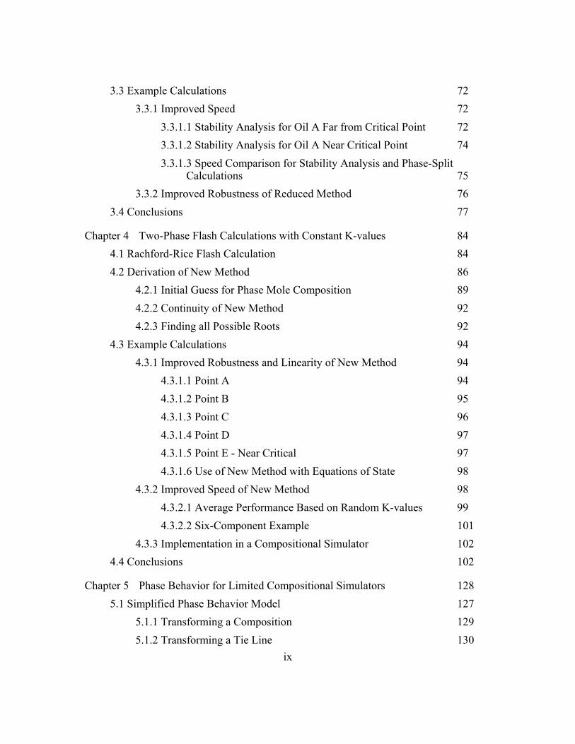
ix
3.3 Example Calculations 72 3.3.1 Improved Speed 72
3.3.1.1 Stability Analysis for Oil A Far from Critical Point 72 3.3.1.2 Stability Analysis for Oil A Near Critical Point 74 3.3.1.3 Speed Comparison for Stability Analysis and Phase-Split
Calculations 75 3.3.2 Improved Robustness of Reduced Method 76
3.4 Conclusions 77
Chapter 4 Two-Phase Flash Calculations with Constant K-values 84 4.1 Rachford-Rice Flash Calculation 84 4.2 Derivation of New Method 86
4.2.1 Initial Guess for Phase Mole Composition 89 4.2.2 Continuity of New Method 92 4.2.3 Finding all Possible Roots 92
4.3 Example Calculations 94 4.3.1 Improved Robustness and Linearity of New Method 94
4.3.1.1 Point A 94 4.3.1.2 Point B 95 4.3.1.3 Point C 96 4.3.1.4 Point D 97 4.3.1.5 Point E - Near Critical 97 4.3.1.6 Use of New Method with Equations of State 98
4.3.2 Improved Speed of New Method 98 4.3.2.1 Average Performance Based on Random K-values 99 4.3.2.2 Six-Component Example 101
4.3.3 Implementation in a Compositional Simulator 102 4.4 Conclusions 102
Chapter 5 Phase Behavior for Limited Compositional Simulators 128 5.1 Simplified Phase Behavior Model 127
5.1.1 Transforming a Composition 129 5.1.2 Transforming a Tie Line 130

x
5.1.3 Flash Calculations Using Transformation Factors 131 5.1.3.1 Linear Model 133 5.1.3.2 Quadratic Model 134 5.1.3.3 Reverse Quadratic Model 135
5.1.4 Reference Component in Transformation Method 136 5.1.5 Calculation Procedure 136
5.2 Stability Analysis in Transformation Model 137 5.3 Example Flash Calculations 138
5.3.1 A C2-nC4-nC10 Ternary Synthetic Oil 138 5.3.2 Surfactant Flooding 139 5.3.3 Phase Behavior at Multiple Pressures 140 5.3.4 Flash Calculations with Limited Data 142 5.3.5 Implementation with Real Fluid Experimental Data 143 5.3.6 Flash Calculations with Constant K-values 144 5.3.7 Simulation Comparison 145
5.4 Conclusions 147
Chapter 6 Conclusions and Future Work 191 6.1 Key Conclusions 191
6.1.1 EOS-Based Reduced Method 191 6.1.2 Constant K-value Flash Calculations 192 6.1.3 Transformation Method for Limited Compositional Simulators 193
6.2 Future Work 197 Appendix Flash Calculations with Negative Compositions 198
Glossary 203
Bibliography 206
Vita 211

xi
List of Tables
Table 2.1: Input EOS properties for synthetic oil A. ....................................................49
Table 2.2: Binary interaction parameters for synthetic oil A. All BIPs not shown
are zero. ........................................................................................................50
Table 2.3 Values for ih and ig for gas condensate B (Jutila et al., 2001) at 275oF
that give a sufficient fit to the original BIPs. The new BIPs calculated
with Eqs. (2.5) are shown. All BIPs not given are zero. ..........................51
Table 2.4: Values for ih and ig for oil C (Hearn and Whitson, 1989) that give a
good fit to the original BIPs. The new BIPs calculated with Eqs. (2.5)
are shown. All BIPs not given are zero. ...................................................52
Table 2.5: Input EOS properties for oil D. ....................................................................53
Table 2.6: Input binary interaction parameters for oil D. Values are given for ih
and ig that give an exact fit to the original BIPs associated with CO2.
All BIPs not given are zero. ........................................................................54
Table 4.1: K-values and overall compositions for a six-component fluid that is near
a critical point. ...........................................................................................104
Table 4.2: K-values and overall compositions for a six-component fluid far from a
critical point. ...............................................................................................105
Table 4.3: Comparison of the number of iterations by the Rachford-Rice method
(1952) and the new objective function in simulations with GPAS
(Okuno, 2007). ..........................................................................................106
Table 5.1: Input EOS critical properties for the ternary system in Fig. (5.1). ............148

xii
Table 5.2: Comparison of the phase envelope in Fig. (5.1) by Peng-Robinson EOS
(1977, 1978) with the new method. With the transformation method,
the relatively difference is usually less than 1% of the EOS equilibrium
compositions, with the maximum less than 4%. TM indicates
“Transformation Method”. ........................................................................149
Table 5.3: Input EOS critical properties for the ternary system in Fig. (5.8). ............150
Table 5.4: Experimental data used in the transformation method in Section (5.3.5).
Four tie lines (in grey) are used to initialize the calculation. All other
data are used to illustrate the accuracy of the non-iterative
transformation method. .............................................................................151
Table 5.5: Initial oil composition and injection gas composition in the UTCOMP
simulation for a ternary system. ................................................................152
Table 5.6: Comparison of CPU time using standard UTCOMP with the
transformation method. The simulation using the transformation
method is much faster. TM means “Transformation Method.” ..............153

xiii
List of Figures
Figure 1.1: A ternary system without a critical point. K-values for the tie lines are
compositional dependent. ............................................................................18
Figure 1.2: Ternary diagram with a critical point. K-values along different tie lines
are compositional dependent. The critical point is shown by the solid
circle. ...........................................................................................................19
Figure 1.3: Constant K-value approximation for the ternary system shown in Fig.
(1.1). The original tie lines and binodal curves are shown in grey, and
the current simplification is shown in black. ..............................................20
Figure 1.4: Phase behavior model of Tang and Zick (1985). In this model, all tie
lines go to the pivot composition (the dead oil pseudocomponent). The
original phase envelope is shown in grey, and Tang and Zick’s binodal
curves in black. ............................................................................................21
Figure 1.5: Phase behavior model of Tang and Zick (1985). In this model, all tie
lines go to the pivot composition (the dead oil pseudocomponent). The
original phase envelope is shown in grey, and Tang and Zick’s binodal
curves in black. ............................................................................................22
Figure 1.6: Ternary diagram described by Hand’s simplification (1930). The
solution requires iteration of the non-linear equations that fit the Hand’s
plot. ..............................................................................................................23
Figure 1.7: Ternary diagram described by Hand’s model that requires no iterations.
The critical point is at the apex where all tie lines intersect. The ratios
of specified compositions have a unit slope. ...............................................24

xiv
Figure 1.8: Ternary diagram for C1-nC4 –nC10 at 2000 psia and 150oF. The critical
point is shown by the black circle. ..............................................................25
Figure 1.9: Hand’s plot for the ternary diagram in Fig. (1.8) after Welch
modification (1982). The data clearly do not have constant slope as
required by Hand’s plot (1930). ................................................................26
Figure 2.1: Flow chart for conventional flash calculation. ............................................55
Figure 2.2: Flow chart for new rapid flash calculation. ..................................................56
Figure 2.3: Speedup for oil A, where the overall composition is far from the critical
locus. . ...........................................................................................................57
Figure 2.4: Speedup for oil A, where the overall composition is near the critical
locus. ...........................................................................................................58
Figure 2.5: Comparison of calculated phase envelopes for gas condensate B (Jutila
et al., 2001) to that generated by PVTSIM (Calsep, 2005). The new
rapid flash method accurately reproduces the saturation pressures. ........59
Figure 2.6: Comparison of calculated solution gas-oil ratios for gas condensate B
(Jutila et al., 2001) at 275oF to that generated by PVTSIM (Calsep,
2005). The characterization with the new rapid flash method is very
accurate. ......................................................................................................60
Figure 2.7: Comparison of calculated formation volume factors for gas condensate
B (Jutila et al., 2001) at 275oF to that generated by PVTSIM (Calsep,
2005). The characterization with the new rapid flash method is very
accurate. .....................................................................................................61

xv
Figure 2.8: Comparison of calculated phase envelopes for oil C (Hearn and
Whitson, 1995) to that generated by PVTSIM (Calsep, 2005). The
characterization with the new rapid flash method accurately reproduces
the saturation pressures. ..............................................................................62
Figure 2.9: Comparison of calculated solution gas-oil ratios for oil C (Hearn and
Whitson, 1995) at 212oF to that generated by PVTSIM (Calsep, 2005).
The characterization with the new rapid flash method is very accurate. ..63
Figure 2.10: Comparison of calculated formation volume factors for oil C (Hearn and
Whitson, 1995) at 212oF to that generated by PVTSIM (Calsep, 2005).
The characterization with the new rapid flash method is very accurate. ....64
Figure 3.1: Comparison of the total computation time for both the reduced method
and the conventional method in stability analysis as a function of the
number of pseudocomponents for oil A. For seven components, the
speedup from the conventional method is approximately 1.9 and for 35
components, the speedup is 23 (Okuno, 2007). ..........................................78
Figure 3.2: Comparison of the computation time for stability analysis per NR
iteration for oil A that is far from a critical point. Both the reduced and
the conventional methods are tested. As shown, the reduced method is
significantly faster (Okuno, 2007). .............................................................79
Figure 3.3: Comparison of the total computation time for stability analysis and
phase-split calculations using reduced method for oil A. The stability
analysis is approximately three times faster. In this case, the oil is far
from a critical point (Okuno, 2007). ...........................................................80

xvi
Figure 3.4: Comparison of the computation time per iteration for stability analysis
and phase-split calculations using the reduced method for oil A. The
stability analysis in reduced space is moderately faster than the phase-
split calculation in reduced space. In this case, the oil is far from a
critical point (Okuno, 2007). .......................................................................81
Figure 3.5: Comparison of the total computation time for oil A near a critical point.
Both the reduced and the conventional methods are used. The reduced
method is much faster than the conventional one (Okuno, 2007). ..............82
Figure 3.6: Comparison of the computation time for stability analysis per NR
iteration for oil A near a critical point. The reduced method is
significantly faster and requires fewer iterations (Okuno, 2007). ...............83
Figure 4.1: Ternary diagram with K1 =5.0 , K2 =2.0 , and K3 =0.5 . The four
compositions shown all lie on the same tie line and its extension. ...........107
Figure 4.2: Rachford-Rice function (1952) for point A in Fig. (4.1). The red
vertical lines are the limits of the window given by Whitson and
Michelsen.(1989) The correct root within that window is shown by the
solid dot. There are three poles. ..........................................................108
Figure 4.3: Objective functions for point A based on our new method and that given
by Wang and Orr. (1997, 1998) The correct root lies within the
window given by Eq. (4.13). The new objective function is highly
linear. .........................................................................................................109
Figure 4.4: Comparison of the number of iterations for convergence as a function of
the initial guess for both Rachford-Rice (1952) and the new function in
Eq. (4.12). The values of V shown for the new function lie in the
window of Eq. (4.13). ...............................................................................110

xvii
Figure 4.5: Rachford-Rice function (1952) for point B in Fig. (4.1). The root
shown is for the tie line at the base of the ternary diagram, but it does not
lie within the Whitson-Michelsen (1989) window. Thus, convergence
is not guaranteed. ......................................................................................111
Figure 4.6: Objective function for point B based on our new method. The function
by Wang and Orr (1997, 1998) cannot be plotted because z1 is 0.0. Our
function, however, gives the correct root for the tie line through point A.
The window of Eq. (4.13) is also shown. ..................................................112
Figure 4.7: Rachford-Rice (1952) function for point C in Fig. (4.1). The root
shown lies within the Whitson-Michelsen window (1989). The solution
is greater than 1.0 because it is outside the two phase region where only
vapor exists. ...............................................................................................113
Figure 4.8: Objective functions for point C based on our new method and that given
by Wang and Orr (1997, 1998). The correct root lies within the
window given by Eq. (4.13). .....................................................................114
Figure 4.9: Rachford-Rice (1952) function for point D in Fig. (4.1). There is no
root within the Whitson-Michelsen (1989) window. Outside the
window, there is a root, but it is nonphysical, i.e. one equilibrium phase
composition is negative. ..........................................................................115
Figure 4.10: Objective functions for point D based on our new method and that given
by Wang and Orr (1997, 1998). The correct root lies just within the
window given by Eq. (4.13), while only the trivial root exists for Wang
and Orr (1997, 1998). ..............................................................................116

xviii
Figure 4.11: Ternary phase behavior with K1 =1.0+2ε, K2 =1.0+ε, and K3 =1-ε and
ε=10-9. The two phase region shown is very small and appears as a line
in this diagram. The solid line is the tie-line extension through E. ........117
Figure 4.12: Rachford-Rice (1952) function for point E in Fig. (4.11). The correct
root lies within the Whitson-Michelsen (1989) window. ..........................118
Figure 4.13: Objective functions for point E based on our new method and that given
by Wang and Orr (1997, 1998). The correct root lies within the
window given by Eq. (4.13). Wang and Orr’s method (1997, 1998)
could mistakenly converge to the trivial root. ...........................................119
Figure 4.14: Ternary diagram at 1015 psia and 440 oF for C1-C6-C10 system. Flash
calculations with Peng-Robinson EOS (1977, 1978) converge to overall
compositions within double precision values of the critical point (see
triangular region). ......................................................................................120
Figure 4.15: Comparison of the average CPU time for one flash calculation as a
function of the number of components in the fluid. The new method is
significantly faster than both Rachford-Rice (1952; Whitson and
Michelsen, 1989) and Leibovici-Neoschil (1992). ...................................121
Figure 4.16: Comparison of the average number of iterations required for
convergence for each method as a function of the number of
components. Leibovici-Neoschil (1992) and the new method give
about the same number of iterations. ........................................................122
Figure 4.17: Comparison of the average CPU time per iteration for each method as a
function of the number of components. The new method is much faster
than Leibovici-Neoschil (1992), but slower than Rachford-Rice (1952;
Whitson and Michelsen, 1989). ................................................................123

xix
Figure 4.18: Rachford-Rice (1952) function for the K-values and overall composition
given in Table (4.1). The function is highly nonlinear and the root lies
just within the Whitson-Michelsen (1989) window (red vertical lines)
near the pole. .............................................................................................124
Figure 4.19: Objective functions for the fluid given by Table (4.1) based on our new
method and that given by Wang and Orr (1997, 1998). The correct
root lies just within the window given by Eq. (4.13). Wang and Orr’s
method (1997, 1998), however, could converge to the trivial root. ..........125
Figure 4.20: Rachford-Rice (1952) function for fluid given by Table (4.2).
Convergence for V requires 18 iterations for an initial guess of 0.5.
Convergence is difficult because the function is nonlinear and the root is
near the right window limit. ......................................................................126
Figure 4.21: The objective function for the new method based on the fluid in Table
(4.2). Convergence is achieved in 6 iterations even though the root is
near a pole. The pole is just outside the window given by Eq. (4.13). ....127
Figure 5.1: Ternary diagram for C2-nC4-nC10 system at 498.03 K and 6.125 MPa.
The equilibrium compositions are calculated using the Peng-Robinson
EOS (1977, 1978). ...................................................................................154
Figure 5.2: Ternary diagram for C2-nC4-nC10 system in the transformed space at
498.03 K and 6.125 MPa. The transformation factor is applied to the
C2 component. In the transformed space, all tie lines are parallel, and
the critical point occurs when *4nC is a maximum. .................................155
Figure 5.3: Transformation factors for C2-nC4-nC10 ternary system in Fig. (5.1). A
quadratic function is very accurate to describe the curve. ......................156

xx
Figure 5.4: Transformation factors for C2-nC4-nC10 ternary system in Fig. (5.1).
The solid line uses the quadratic function, the dash line is that from Eq.
(5.2) for an overall composition. The triangle is the correct
transformation factor for the tie line passing through the overall
composition. ............................................................................................157
Figure 5.5: Comparison of the equilibrium compositions for C2-nC4-nC10 system at
498.03 K and 6.125 MPa. The calculated values are in black, and the
original data are in grey. The new non-iterative method yields almost
identical results. .........................................................................................158
Figure 5.6: Ternary diagram in the transformed space for C2-nC4-nC10 system. The
transformation factor is applied to the nC10 component. The critical
point occurs at the largest *4nC composition. ..........................................159
Figure 5.7: Transformed nC4 composition as a function of the transformation factor
for the ternary system in Fig. (5.6). The transformation factors are
applied to the nC10 component. An accurate quadratic curve is used in
this case. ....................................................................................................160
Figure 5.8: Equilibrium compositions computed by the transformation method when
the transformation factors are applied to nC10 component. The original
data (gray) are from the Peng-Robinson EOS (1977, 1978). The non-
iterative transformation method yields accurate phase behavior (black)....161
Figure 5.9: Ternary diagram for a brine-oil-surfactant ternary system with co-
surfactant injected (Pope, et al. 1982). The tie lines are in dash lines
and the original data are in triangles. ........................................................162
Figure 5.10: Transformation factors for a surfactant system (see Fig. (5.9)). The
transformation is applied to the oil component. ........................................163

xxi
Figure 5.11: Comparison of the non-iterative transformation method (diamonds with
tie lines) with the experimental data (triangles). .......................................164
Figure 5.12: Hand’s plot (1930) for the ternary diagram of chemical flood in Fig.
(5.9). ..........................................................................................................165
Figure 5.13: Comparison of Hand’s method (diamonds with tie lines) and the
experimental data (triangles). Hand’s method is less accurate than the
trasformation method. ...............................................................................166
Figure 5.14: Ternary diagram for C1- nC4 - nC10 system at different pressures from
2000 psia to 4000 psia at 150oF. The critical points at each pressure are
shown by solid circles. ..............................................................................167
Figure 5.15: Transformed nC4 composition as a function of transformation factor for
the ternary diagram in Fig. (5.14) at different presures. The critical
points is always at the maximum value for *4nC . .....................................168
Figure 5.16: The minimum transformation factor (the critical tie line) and the
maximum (the base tie line) as a function of pressure. The calculated
transformation factors must lie within this range. .....................................169
Figure 5.17: Bubble-point curves in the transformed space at different pressures for
the phase behavior in Fig. (5.14). All curves are regressed accurately
using quadratic functions. .........................................................................170
Figure 5.18: Dew-point curves in the transformed space at different pressures for the
phase behavior in Fig. (5.14). All curves are regressed accurately using
quadratic functions. ...................................................................................171

xxii
Figure 5.19: Equilibrium compositions calculated using the transformation method at
pressure of 3000 psia and 150oF. The transformation method is
accurate. The original data from the PR EOS (1977, 1978) is shown in
grey and the calculated data using the transformed method is in black. ...172
Figure 5.20: Transformed nC4 composition as a function of the transformation factor
for the ternary system in Fig. (5.14) at different pressures. We linearly
interpolate the relationship at each pressure from the base tie line to the
critical tie line in this example. .................................................................173
Figure 5.21: Bubble point curves in the transformed space using linear interpolation
for the oil in Fig. (5.14). .......................................................................174
Figure 5.22: Dew point curves using linear interpolation in the transformed space for
the oil in Fig. (5.14). ..................................................................................175
Figure 5.23: Equilibrium compositions calculated using the transformation method at
3000 psia and 150oF. We linearly interpolate the phase behavior from
the limiting tie line to the base tie line on the 1-3 axis. The
transformation method using linear interpolation yields accurate results. 176
Figure 5.24: Transformed nC4 composition as a function of transformation factor for
the CO2-nC4-C10 ternary system (Metcalfe and Yarborough, 1979) at
1000 psia (diamonds) and 1400 psia (triangles). ......................................177
Figure 5.25: Binodal curves in the transformed space at pressures of 1000 psia
(diamonds) and 1400 psia (triangles). Linear interpolation is used for
the binodal curves between two tie lines at each pressure. .......................178

xxiii
Figure 5.26: Equilibrium compositions calculated at 1000 psia (diamonds) and 1400
psia (triangles) using the transformation method. The experimental
data is shown in dots and the calculated equilibrium compositions are in
curves. The new method predicts the phase behavior accurately. ..........179
Figure 5.27: Equilibrium compositions calculated at 1250 psia (diamonds) and 1500
psia (triangles) using the transformation method. The experimental
data is shown in dots and the calculated equilibrium compositions are in
curves. The new method is accurate. ......................................................180
Figure 5.28: Transformed intermediate composition as function of the transformation
factor for a ternary system with constant K-values of 1 5.0K = ,
1 2.0K = and 3 0.5K = . ...........................................................................181
Figure 5.29: Calculated equilibrium compositions using the transformed method for
the ternary system with constant K-value in Fig. (4.1). Triangles are
from the Rachford-Rice method (1952), and the lines are from the
transformation method. The transformation method is very accurate. ...182
Figure 5.30: Comparison of the C10 recovery using the standard EOS model
(triangles) and the transformation method (lines) at different numbers of
grid blocks. The numbers of grid blocks are 10, 20 and 40,
respectively, from the top. The transformation method agrees well with
the conventional method. ..........................................................................183
Figure 5.31: Comparison of the average reservoir pressure in psia using the standard
EOS model (triangles) and the transformation method (lines). The
number of grid blocks are 10, 20 and 40, respectively, from the top.
The transformation method agrees well with the conventional
simulation. ............................................................................................184

xxiv
Figure 5.32: Comparison of the compositions measured at the production well using
the standard EOS model (triangles) and the transformation method
(curves). The nC4 compositions are in solid lines, nC10 are in dash lines
and C1 are in double dash lines. ................................................................185
Figure 5.33: Comparison of pressure profile at 20 days using 10 (top), 20 (middle)
and 40 (bottom) grid blocks. The standard UTCOMP results are in
triangles and the transformation method results are in curves. The non-
iterative transformation method is almost identical as the conventional
method. ......................................................................................................186
Figure 5.34: Comparison of the pressure profile at 40 days using 10 (top), 20
(middle) and 40 (bottom) grid blocks. The standard UTCOMP results
are in triangles and the transformation method results are in curves.
The non-iterative transformation method is very accurate. ......................187
Figure 5.35: Comparison of the overall composition profile at 20 days using 10 (top),
20 (middle) and 40 (bottom) grid blocks. The standard UTCOMP
results are in triangles. The results using the transformation methods
are: nC4 in solid curves, nC10 in dash curves and C1 in double dash
curves. .......................................................................................................188
Figure 5.36: Comparison of the overall composition profile at 40 days using 10 (top),
20 (middle) and 40 (bottom) grid blocks. The standard UTCOMP
results are in triangles. The results using the transformation methods
are: nC4 in solid curves, nC10 in dash curves and C1 in double dash
curves. .......................................................................................................189

xxv
Figure 5.37: CPU time used for the flash calculations in simulation using the standard
UTCOMP method and the transformation method. The new method is
approximately 10 times faster than the conventional flash calculation. .....190
Figure A.1: Ternary diagram with K1 =5.0 , K2 =2.0 , and K3 =0.5 . The two
compositions shown lie on the same tie-line extension as that point in
Fig. (4.1). ...................................................................................................198
Figure A.2: Rachford-Rice function (1952) for point A in Fig. (A.1). The vertical
lines are the limits of the Whitson-Michelsen window (1989). There
are two roots (solid dots) corresponding to different tie lines and both
are not within that window. ........................................................................199
Figure A.3: Objective functions for point A in Fig. (A.1) based on the new objective
method and that given by Wang and Orr (1997, 1998). The two correct
roots (the solid dots) lie within the window given by Eq. (A.7). The
new objective function is very linear. .........................................................201
Figure A.4: Rachford-Rice function (1952) for point B in Fig. (A.1). The vertical
lines are the limits of the Whitson-Michelsen window (1989). The
correct root (solid dot) is not within the window........................................202
Figure A.5: Objective functions for point B in Fig. (A.1) based on the new objective
method and that given by Wang and Orr (1997, 1998). The correct root
(the solid dot) lies within the window given by Eq. (A.7). The new
objective function is very linear..................................................................203

1
Chapter 1: Introduction
Enhanced oil recovery (EOR) processes will be very important to lessen the gap
between oil supply and demand. Many EOR processes, such as gas injection, result in
complex interactions of flow with phase behavior. This is mainly because reservoirs are
operated at conditions where miscibility is developed between the injection gas and the
reservoir fluid. Depending on production pressure and gas composition, there are two
different miscibility mechanisms: first-contact miscibility (FCM) and multi-contact
miscibility (MCM). For FCM, the reservoir hydrocarbon is miscible with the injection
gas in any proportion so that a piston-like or quasi-piston-like displacement occurs.
First contact miscible displacements often require very high pressures that are usually not
obtainable. For MCM, miscibility is developed in situ by repeated contacts between the
injection gas and the reservoir fluid. Compositional changes are the important driving
force for enhanced recovery, and distinguish gas injection from immiscible water floods.
Reservoir simulation is often performed to evaluate the oil reservoirs and
production strategies, and to give valuable insights into the displacement mechanisms.
Despite simplicity and speed, black oil models are typically too simple to accurately
account for the compositional changes that occur in gas flooding simulations. Since
most EOR processes are compositional in nature, we need compositional simulations to
model them.
In compositional simulation, we need to solve for the following at each time step
for each grid block: (1) When the injection solvent contacts with the reservoir fluid, does
the mixture split into multiple phases or not? (2) If the overall composition is not stable,
how many phases will form? (3) For each phase, what are the equilibrium
compositions? (4) What are the phase saturations and densities? Equations-of-state

2
(EOS) are used to test the stability of a single-phase mixture and also to determine
equilibrium compositions by flash calculations if Np>1. The first two questions are
answered with stability analysis calculations, and the remaining with phase-split
calculations.
A significant disadvantage of fully compositional simulations, however, is that
they are much more computationally intensive than black-oil simulations. Thus there is
a great need for faster and more robust compositional simulators. The primary reason
for the increased computational time is the result of solving iterative flash calculations in
each time step for each grid block. For example, for an IMPEC (implicit pressure
explicit compositions) type simulation with grid blocks of 200 × 200 × 25 and 2000 time
steps, about two billion flash calculations are performed. A linear solver to update
reservoir pressure for the same case would be done 2000 times. In general, flash
calculations using cubic EOS can occupy a significant percentage of total computational
time in IMPEC compositional simulations (Stenby and Wang, 1993; Chang, 1990).
Repeated flash calculations with cubic EOS are also needed in other problems
such as multi-phase flow in pipelines (Lityak and Wang, 1998) and determination of
minimum miscible pressure (MMP) or minimum miscible enrichment (MME) by an
analytical method (Jessen et al., 1998; Yuan and Johns, 2005).
There are a few standard methods used to reduce computation time in flash
calculation. The first is to use fewer pseudocomponents. However, this approach
results in less accuracy and requires significantly more tuning (Hong, 1982; Liu 2001;
Egwuenu et al. 2005). This is especially true in MCM displacements, in which
miscibility is developed by a combined condensing/vaporizing (CV) drive process (Zick,
1986; Johns et al., 1992; Johns et al. 1993; Johns and Orr, 1996). Fluid characterization
for these models can be improved by tuning to the analytical MME or MMP (Egwuenu et

3
al. 2005), but those models still require significant computational time even with fewer
pseudocomponents.
Another way to decrease computation time is to reduce the number of grid blocks.
With coarser grids, however, numerical dispersion is unrealistically large, which will
result in poor prediction from simulation (Solano et al. 2001). Ideally, fine grids should
be used that can better match the level of dispersion found at field scale.
In this dissertation, we focus on three different approaches for rapid calculations:
(1) phase-split calculations and stability analysis using EOS models; (2) constant K-value
models, and (3) simplified phase behavior models for limited compositional simulation.
1.1 TWO-PHASE SPLIT CALCULATIONS USING EQUATIONS-OF-STATE
In compositional simulation, we often assume that the reservoir fluid and injection
gas are at thermodynamic equilibrium in each grid block at each time step. Equilibrium
compositions depend on reservoir temperature, pressure and overall composition given
by mass balance equations (governing equations in IMPEC type reservoir simulators).
Two distinct methods are used to calculate equilibrium compositions. The first is to
minimize Gibbs free energy of the mixture, because Gibbs free energy should be a
minimum when the mixture is at equilibrium (Heidemann, 1974; Gautam and Seider,
1979; Trangenstein, 1985). The other uses the equality of fugacity for each component
at different phases and solves these nonlinear fugacity equations to find equilibrium
compositions (Michelsen, 1982a, 1982b). In conventional flash calculations, there are
CN primary variables, for example equilibrium K-values for each pseudocomponent,
where CN is the number of pseudocomponents. As a result, the speed of flash
calculations usually decreases quadratically as a function of CN .

4
More recently, reduced methods are of growing interest, because they can
significantly decrease the number of primary variables for flash calculations, and thus
greatly save computation time. In these methods, we can write excess Gibbs energy and
fugacities in terms of a few groups that are called reduced parameters or reduced
variables.
For example, when all binary interaction parameters (BIPs) are zero, the speed of
phase-split calculations can be significantly improved by finding three reduced
parameters using the standard van der Waals mixing rules (Michelsen, 1986). The
number of primary variables is therefore independent of the number of
pseudocomponents. The assumption of all zero BIPs is not realistic, however, when
CO2, nitrogen or other non-hydrocarbon components are injected or present.
Jensen and Fredenslud (1987) extended Michelsen’s approach (1986) by using
two more reduced parameters when only one column of the BIP matrix is non-zero. For
example, when CO2 is injected, they obtained five reduced parameters. All other BIPs
between the remaining components, however, must be zero, which again limits its
usefulness. Their method quickly becomes cumbersome when there are many
pseudocomponnets with non-zero BIPs. For an CN -component system, if there are m
columns or rows in the BIP matrix that have non-zero elements, the total number of
reduced parameters is 2 3m + . When m is large, the number of reduced parameters can
be a large value, and thus no or little improvement in speed compared with the
conventional method.
Recently, a different diagonalization method for the BIP matrix is proposed using
linear transformation techniques (Nichita, 2006). This model solves a set of linear
functions for the BIP matrix. Although this method maintains the diagonal BIP
elements, it provides no further reduction compared with the model developed by Jensen

5
and Fredenslund (1987). We still need 2 3m + reduced variables for m components
that have non-zero BIPs with other components (Jensen and Fredenslund, 1987; Nichita
and Minescu, 2004; Nichita, 2006).
Hendricks (1988) used an eigenvalue analysis method to identify the dominant
BIPs in phase-split calculations. The binary interaction parameter matrix is
recalculated by setting all small eigenvalues to be zero, using some predetermined
criterion (that are often uncertain). Hendricks and van Bergen (1992) later applied this
procedure using Newton-Raphson (NR) iteration. Although this method is faster than
conventional flash calculations, zeroing of eigenvalues can lead to non-physical BIPs in
that the diagonal elements of the BIP matrix have small nonzero values. In addition,
their method is only an approximation at its best to the original phase behavior
characterization. Pan and Firoozabadi (2001) formulated phase-split calculations using
the same reduced parameters of Hendricks (1988) with a general cubic EOS (Coats,
1985).
The comparison of the BIP modeling methods (Michelsen, 1986; Jensen and
Fredenslund, 1987; Nichita, 2006) and the dominant eigenvalue decomposition methods
(Hendricks, 1988; Pan and Firoozabadi, 2001; Nichita et al. 2004) from the previous
research indicates that: (1) both approaches significantly reduce the number of primary
variables. Dominant eigenvalue decomposition methods require the elimination of small
eigenvalues to achieve this objective, while BIP modeling methods require a strong
interrelationship in BIP elements. (2) Dominant eigenvalue decomposition is only an
approximation at its best, and may often lead to non-zero diagonal BIPs. (3) If BIPs are
required to change frequently as reservoir pressure and temperature change, determining
the dominant eigenvalue is required for each grid block in each time step. As a result,
this method can be very computationally intensive. (4) BIP modeling method may

6
provide easier and systematically accurate regression than dealing with individual BIP
elements. The regression process is empirical subject to experience, but a strong
interrelationship, although still ambiguous, may be an appropriate approach accounting
for the physical forces between hydrocarbon molecules.
The global minimization method for flash calculations can also be applied in both
actual compositional space (Nagarayan et al., 1991; Bullard and Biegler, 1993, Han and
Rangaiah 1997) and reduced space (Pan and Firoozabadi, 1998; Firoozabadi, 1999;
Nichita et al., 2002). These methods are of great value and some reservoir simulators
use these methods (only available in actual compositional space) over direct solution
methods. For simplicity and better speed, however, we only consider direct solution
methods to calculate equilibrium compositions in this dissertation. In addition, the
purpose of this dissertation is not to examine the difference by using various iterative
methods, but to propose a practical EOS model for compositional simulators. This new
EOS model can be optimized by applying different iterative techniques, which may be a
topic of future research.
1.2 STABILITY ANALYSIS CALCULATIONS USING REDUCED METHOD
Stability analysis is very important in reservoir simulations because slow phase-
split calculations that are unnecessary can be eliminated. In addition, stability analysis
can often provide a better initial guess for phase-split calculations. Stability analysis
should be done for each grid block at each time step. As a result, phase-split
calculations are performed only when (1) stability analysis shows that the mixture of the
reservoir fluid and injection gas is unstable; or (2) the grid block has multiple phases in
the previous time step (Voskov and Tchelepi, 2007).
7
Similar to phase-split calculations, there are two different approaches for stability
analysis. The first approach focuses on finding the minimum of the tangent plane
distance (TPD) function and the second focuses on finding the stationary points of TPD
and then evaluates the TPD values at those stationary points. The tasks are similar in
both approaches. In the first approach, we need to find the global minimum rather than
local minima. In the second approach, we need to locate all the stationary points.
Baker et al. (1982) examined the Gibbs free energy surface and the tangent plane
to that surface at calculated equilibrium compositions. When the Gibbs free energy
surface is always above the tangent plane, tangent points are the correct equilibrium
solutions. When Gibbs free energy surface is below the tangent plane at any
composition, the equilibrium solution is incorrect, although that solution satisfies both
mass balance and equal-fugacity constraints.
Further based on this Gibbs free energy analysis, Michelsen (1982a) formulated
phase stability analysis by calculating the distance between Gibbs free energy surface and
the tangent plane, called the tangent plane distance (TPD). Stability analysis is to locate
the minimum of the TPD at all compositions. He further suggested that the check of
positivity at stationary points is sufficient. In addition, Michelsen (1982a) suggested
that it is sufficient to determine the stationary points by the initial guesses using a
composition made up of either the most or least volatile components. This approach is
widely used in stability analysis calculations owing to its simplicity.
Hua et al. (1996) found all stationary points of the TPD by an interval
Newton/Bisection method. However, their approach requires significant calculations
because the actual compositional space is divided into many small sub-domains and
Newton/Bisection calculations are then applied in each of them. This approach is very

8
expensive in reservoir simulations because billions of these stability analysis calculations
are executed.
Rasmussen et al (2006) identified a problematic region for stability analysis
calculations, which is located close to the two-phase boundary. In this region, a slight
overshooting of the Newton step may force convergence to the trivial solution where
i iy z= rather than to the correct solution.
All the methods above used compositions of the trial phase as primary variables.
That is, an CN -component system requires CN primary variables. As a result, stability
analysis calculations are still relatively very slow.
Some researchers have extended stability analysis calculations in reduced space
by the dominant eigenvalue decomposition of the BIP matrix using Lagrange multipliers
(Firoozabadi and Pan, 2002) or direct solution methods (Nichita et al. 2004; Hoteit and
Firoozabadi, 2006). In addition, Hoteit and Firoozabadi (2006) also identified the trivial
solution problem mentioned by Rasmussen et al. (2006) in reduced space. Nevertheless,
they showed that the reduced method is much faster with a speedup ratio that depends on
the number of pseudocomponents. This is mainly because the reduced method uses
significantly less primary variables and thus a much smaller Jacobian matrix (in direct
solution approach) or Hessian matrix (in minimization approach).
The global minimization method, although not a topic in this dissertation, has
attracted some interest as well to be used both in actual compositional space (McDonald
and Floudas, 1995; Sun and Seider, 1995; Hua et al., 1996; Hua et al., 1998; Harding and
Floudas, 2000) and in reduced space (Firoozabadi and Pan, 2002; Nichita et al., 2002;
Nichita et al. 2006). Stability analysis calculations that are currently performed in
reduced space employ the same reduced variables using the dominant eigenvalue
decomposition method as described by Hendricks and van Bergen (1992). Firoozabadi

9
and Pan (2002) also observed that the TPD surface is smoother in the reduced space than
in compositional space. Because of the same concern we have in phase-split calculation,
we only focus on direct solution methods in this study.
1.3 PHASE-SPLIT CALCULATIONS USING REDUCED METHOD FOR THREE OR MORE PHASES.
Phase-split calculations for three or more phases have important applications as
well. For example, CO2 injection can result in the formation of three hydrocarbon
phases — two oleic phases and one gaseous phase — under realistic reservoir
temperatures and pressures.
Conventional phase-split calculations can be extended to three or more phases.
However, for an CN -component system with PN phases, the conventional method
requires iterations on ( )1P CN N− primary variables, i.e., the K-values of each
component in each phase (expect those in the reference phase). As a result, phase-split
calculations are much slower than that in the two-phase region. This is mainly because
of the significantly increased size of the Jacobian matrix.
We can also extend the reduced method to phase-split calculations in three or
more phases, similar to that in two-phase flash calculations. Since the number of
primary variables is greatly lowered compared with conventional flash calculations, the
speedup could be much more than two-phase flash calculation.
Nichita et al. (2005) used the same reduced parameters as described by Hendricks
and van Bergen (1992) for phase-split calculations in three or more phases. They
showed that, similar to that in two-phase flash calculations, both computation speed and
robustness are significantly increased compared with the conventional phase-split
method.

10
1.4 FLASH CALCULATIONS WITH CONSTANT K-VALUES
Flash calculations with constant K-values play an important role as well in
reservoir simulations in that: (1) in each of the conventional flash step 5, we need to use
this iterative routine to update K-values; (2) for grid blocks where pressure is much lower
than MMP, constant K-values is a good approximation for the phase behavior. Constant
K-value flash calculations are much faster than EOS flash calculations. Even though
this flash calculation is easier to formulate than EOS flash calculations, there are potential
problems that can lead to the wrong solutions.
Rachford and Rice (1952) derived a simple objective function assuming constant
K-values to calculate phase compositions for two equilibrium phases. They used an
iterative bisection method where phase molar fraction, either the liquid phase or the vapor
phase, is constrained to lie in the range from 0.0 to 1.0. Equilibrium phase compositions
are then calculated by mass balance equation from the converged phase saturation and
overall compositions. The objective function of Rachford and Rice (1952), however,
has many poles and roots and is often very nonlinear. As a result, the convergence to
the correct root by bisection method can be very slow. Further, when the overall
composition lies outside the two-phase zone, the correct root is not between 0.0 and 1.0.
Li and Nghiem (1982) extended the Rachford-Rice method (1952) to negative
flash calculations, where the overall composition can be outside two-phase zone, but
within the region of tie-line extensions. They also improved the speed of convergence
by using Newton-Raphson (NR) iterations. There is no guarantee with their method,
however, that NR will converge to the correct root because of the multiplicity of poles
and roots.

11
Whitson and Michelsen (1989) made a significant improvement in the robustness
of negative flash calculation by specifying a range or window in which the correct root of
the phase molar fraction should lie. Furthermore, they showed that there are no poles
within that range. Because of the nonlinearity of the Rachford-Rice (1952) objective
function, however, their improvement still suffers from many of the same disadvantages
as the original Rachford-Rice method (1952).
Several authors (Von Rossenberg, 1963, 1977; Warren and Adewumi, 1993;
Monroy-Loperena and Vargas-Villamil, 2001) derived a new objective function by
multiplying the Rachford-Rice (1952) function by its denominators (poles). This
approach makes the new objective function more continuous than the Rachford-Rice
objective function (1952). However, this objective function is much more
computationally intensive and nonlinear than the original Rachford-Rice (1952) function.
Thus, this approach offered no significant advantages over the Rachford-Rice (1952)
function with the Whitson and Michelsen (1989) window.
Leibovici and Neoschil (1992) continued this approach. They multiplied the
Rachford-Rice objective function (1952) by the denominators of poles corresponding to
the lightest and heaviest components, instead of all the pseudocomponents. They gave a
smaller window for phase mole fraction than that of Whitson and Michelsen (1989) and
showed some improvement in average computational time for the flash calculations
considered. Their method, however, still has problems with the nonlinearity of the
objective function, especially when the lightest and heaviest components are present in
small amounts and the overall composition is close to either the bubble-point or dew-
point curves. Their method also suffers from increased computational cost per iteration
and in most cases of practical interest will not be faster than Rachford-Rice (1952).

12
Last, their method cannot be extended to equilibrium calculations with more than two
phases (Leibovici and Neoschil, 1995), and is therefore not a general approach.
Wang and Orr (1997, 1998) used the same Rachford-Rice (1952) objective
function, but iterated on the liquid equilibrium phase composition of the lightest
component ( 1x ) instead of vapor phase molar fraction. Their goal was primarily to
improve the convergence for overall compositions outside of positive composition space
where at least one overall composition is negative. For practical flash calculations,
however, their method is similar to that of Rachford-Rice (1952). In addition, this
approach suffers from a trivial solution at 1 0x = .
1.5 LIMITED COMPOSITIONAL RESERVOIR SIMULATION
Comparison of EOS compositional simulators and black-oil models indicates that
the difference in computational time of a simulation largely depends on phase behavior
calculations. In EOS compositional simulators, equilibrium phase compositions are
calculated iteratively by solving equal-fugacity equations. In black-oil models, phase
behavior calculations are much faster using some simple relationships, for example,
solubility as a function of the pressure.
There are many simulation projects that black-oil models are inappropriate to use
even though they are faster than compositional models. For example, in CO2
sequestration in an oil reservoir, the phase behavior is often considerably much more
complicated than that used in black-oil models. However, the reservoir itself may
require so many grid blocks and time steps that prohibit the use of expensive EOS
compositional simulators. Even if we can lump the reservoir fluids using only a few
pseudocomponents or use reduced methods, flash calculations are still iterative, and thus
fully compositional simulation is still slow. It is obvious that an accurate non-iterative

13
phase behavior model is very desirable. One approach is to use simplified phase
behavior models for a limited number of pseudocomponents, but where the key
compositional effect such as vaporization are retained.
Limited compositional reservoir simulators (LCRS) could be used to fill the gap
between EOS compositional and black-oil models. There are some three- or four-
components LCRS available, and the major difference among them is usually the phase
behavior calculations. The required flash calculations for each grid block must be: (1)
very efficient in that no fugacity calculations should be used to determine equilibrium
compositions; (2) very fast in that no or only a few iterations are needed in flash
calculations; (3) unique in that only the correct solution(s) can be determined for any
given overall composition, and no tie line can intersect in the multi-phase region; and (4)
reasonably accurate in that the intersection of tie lines and binodal curves (bubble point
and dew point curves) can represent experimental data or EOS flash calculation results.
There are two different pieces of information required to calculate equilibrium
phase compositions. One is for the shape of the binodal curves and the other is for the
slope of the tie line passing through the specified overall composition. In LCRS, both
information is significantly simplified, so that direct solution is possible.
One common practice is compositionally independent K-values, which are the
ratio of equilibrium vapor compositions to liquid compositions. This type of flash
calculation is outlined in section (1.4), and in more detail in Chapter 4 for a newly
developed model. In this type of model, the binodal curves are straight lines (or plains),
and the tie lines are defined by these K-values (Fig. (1.3)). However, we still need
iterations for equilibrium computations using this model, although the calculation is
much faster compared with EOS compositional model because only one primary variable
is used for the two-phase flash calculations. Flash calculations with compositionally

14
independent K-values are sometimes good approximations when reservoir pressure is
significantly lower than MMP (and thus it is immiscible flood or when the composition
path avoids the critical region.), for example, for the case of ternary systems as shown in
Fig. (1.1). However, when reservoir pressure is greater than the MMP during gas
flooding, it is impossible for these K-values to be compositionally independent. For
example, it is very inaccurate if we assume constant K-values for the ternary system
shown in Fig. (1.2).
Similar approaches include solubility models that can only simulate partial
miscible floods. In solubility models, solvent solubility in the oleic phase is calculated
using a similar way of calculating the solution gas-oil ratio in black-oil models.
However, solubility is no longer defined under miscible flooding conditions. In
reservoir simulation, if the pressure is less than the MMP, we often use these models; and
when the pressure is higher than MMP, we could use Todd-Longstaff mixing rule (1972)
or other approaches to correct for miscibility.
Phase behavior for a ternary diagram could also be simplified by assuming the
dew-point and bubble-point curves are straight lines. For example, a phase envelope with
this assumption is shown in Fig (1.4). There are several major drawbacks of this model:
(1) no critical point can exist. (2) For a single phase composition close to the critical
point, this model mistakenly treats it as two phases, and thus may yield inaccurate results;
and more importantly (3) no tie-line information is given, and thus intensive iterations are
still required.
An alternative approach to model a miscible flood is described by Tang and Zick
(1986) for ternary systems. In their model, tie lines are assumed to converge to a
common point, known as the pivot composition, which is taken to be the dead oil
pseudocomponent. Binodal curves are assumed to be piecewise linear to the critical
15
point as is shown in Fig. (1.5). This model is relatively inaccurate because the pivot
point assumption is usually invalid for most miscible floods. Further, if we use multiple
linear segments, the pressure dependence of these connecting points requires significant
computation time.
1.6 HAND’S METHOD
Another simple representation of binodal curves and tie lines are made by Hand
(1930). He found that certain ratios of equilibrium compositions in a ternary system are
sometimes straight lines on a log-log scale (see Fig. (1.6)). His method to determine
equilibrium compositions generally requires an iterative approach. For some cases,
iterations are not required for example in surfactant flooding, when (1) the critical point
is at one of the apexes; and (2) the binodal curves are symmetric. With these
assumptions, the new phase envelope can be solved directly by a quadratic solver. This
simplified phase behavior is shown in Fig. (1.7).
Hand’s model (1930) requires that two components are fully immiscible with
each other such that the tie line at the bottom extends to both apexes. However, in gas
floods even the most and least volatile components have some mutual solubility. This
limitation, however, can be lifted by altering the apexes of the ternary diagram to the
solubility limits on the base tie line (Welch, 1982). Direct solution also requires that all
tie lines converge to one of the apexes, which may be accurate enough for some
surfactant cases, but not in gas floods. In addition, for a simple ternary gas flooding, it
has been shown that the straight-line assumption in Hand’s plot (1930) is largely
inaccurate. For example, for a ternary system composed of C1, nC4 and nC10 at 2000
psia and 150oF, bubble point and dew point curves are shown in Fig. (1.8). If we

16
implement Hand’s method (1930) on this ternary system, it does not accurately predict
the equilibrium compositions as shown in Fig. (1.9).
In the same paper, Hand (1930) gave another approach to simplify phase
behavior. This approach assumes equilibrium compositions for the intermediate
components are same at fixed temperature and pressure for both phases. This
assumption essentially implies that all tie lines in compositional space have the same
slope, i.e., are parallel. However, this approach is typically invalid for gas flooding or
surfactant flooding cases of practical interest. In this dissertation, we extend this idea
from Hand (1930), however, to model accurately real phase behavior data.
1.7 OBJECTIVES AND OUTLINE OF DISSERTATION
The objective of this research is to develop simple, fast, robust and accurate flash
calculation models that can be applied for compositional simulation. Chapter 2
describes EOS compositional phase-split calculations based on our new reduced method.
We develop a new BIP model that lead to a maximum of six reduced parameters even
when all BIP elements are non-zero. Our research shows that this model is very
accurate compared with other reduced methods. This new model is also significantly
faster than conventional phase-split calculations. We also formulate phase-split
calculations in three or more phases using the same BIP model. In Chapter 3, stability
analysis calculations for EOS compositional simulators based on the same reduced model
are described using a direct Newton-Raphson method. The stability analysis is also
much faster and more robust compared with conventional stability analysis. In Chapter
4, a new phase flash calculation with constant K-values is outlined. This new objective
function is faster and more robust than Rachford-Rice (1952), which is currently used in
most simulators. In Chapter 5, we develop a simplified phase behavior model for

17
ternary systems using a new transformation method. As a result, flash calculations are
non-iterative and can account for different reservoir pressures. Simulation results show
that this model is very accurate compared with EOS models. Last, we draw some
conclusion and outline possible future research.

18
3
1
2
Fig. 1.1 A ternary system without a critical point. K-values for the tie lines are composition dependent.

19
3
1
2
Fig. 1.2 Ternary diagram with a critical point. K-values along different tie lines are composition-dependent. The critical point is shown by the solid circle.

20
3
1
2
Fig. 1.3 Constant K-value approximation for the ternary system shown in Fig. (1.1). The original tie lines and binodal curves are shown in grey, and the current simplification is shown in black.

21
3
1
2
Fig. 1.4 Simplified ternary diagram for Fig. (1.2). The critical point is replaced by a limiting tie-line, and the binodal curves are straight lines. The original phase envelope is shown in grey.

22
3
1
2
Fig. 1.5 Phase behavior model of Tang and Zick (1985). In this model, all tie lines go to the pivot composition (the dead oil pseudocomponent). The original phase envelope is shown in grey, and Tang and Zick’s binodal curves in black.

23
1
23
CP
1
3
CP
31 31
11 21
log vs logC CC C
⎛ ⎞ ⎛ ⎞⎜ ⎟ ⎜ ⎟⎝ ⎠ ⎝ ⎠
32 32
12 22
log vs logC CC C
⎛ ⎞ ⎛ ⎞⎜ ⎟ ⎜ ⎟⎝ ⎠ ⎝ ⎠
32 31
22 11
log vs logC CC C
⎛ ⎞ ⎛ ⎞⎜ ⎟ ⎜ ⎟⎝ ⎠ ⎝ ⎠
Ternary Diagram Hand’s Plot
1
23
CP
1
3
CP
31 31
11 21
log vs logC CC C
⎛ ⎞ ⎛ ⎞⎜ ⎟ ⎜ ⎟⎝ ⎠ ⎝ ⎠
32 32
12 22
log vs logC CC C
⎛ ⎞ ⎛ ⎞⎜ ⎟ ⎜ ⎟⎝ ⎠ ⎝ ⎠
32 31
22 11
log vs logC CC C
⎛ ⎞ ⎛ ⎞⎜ ⎟ ⎜ ⎟⎝ ⎠ ⎝ ⎠
1
23
CP
1
3
CP
31 31
11 21
log vs logC CC C
⎛ ⎞ ⎛ ⎞⎜ ⎟ ⎜ ⎟⎝ ⎠ ⎝ ⎠
32 32
12 22
log vs logC CC C
⎛ ⎞ ⎛ ⎞⎜ ⎟ ⎜ ⎟⎝ ⎠ ⎝ ⎠
32 31
22 11
log vs logC CC C
⎛ ⎞ ⎛ ⎞⎜ ⎟ ⎜ ⎟⎝ ⎠ ⎝ ⎠
Ternary Diagram Hand’s Plot
Fig. 1.6 Ternary diagram described by Hand’s simplification (1930). The solution requires iteration of the non-linear equations that fit Hand’s plot.

24
1
23
1
3
31 31
11 21
log vs logC CC C
⎛ ⎞ ⎛ ⎞⎜ ⎟ ⎜ ⎟⎝ ⎠ ⎝ ⎠
Ternary Diagram Hand’s Plot
1
23
1
3
31 31
11 21
log vs logC CC C
⎛ ⎞ ⎛ ⎞⎜ ⎟ ⎜ ⎟⎝ ⎠ ⎝ ⎠
Ternary Diagram Hand’s Plot
Fig. 1.7 Ternary diagram described by Hand’s model that requires no iterations. The critical point is at the apex where all tie lines intersect. The ratios of specified compositions have a unit slope.

25
C10
C1
nC4
Fig. 1.8 Ternary diagram for C1-nC4 –nC10 at 2000 psia and 150oF. The critical point is shown by the black circle.

26
Fig. 1.9 Hand’s plot for the ternary diagram in Fig. (1.8) after Welch modification (1982). The data clearly do not have constant slope as required by Hand’s plot (1930).

27
Chapter 2: Phase Split Calculations with Reduced Method
In this research, we extend Michelsen’s approach (1986) for fluid
characterizations when all the BIPs are nonzero without resorting to an eigenvalue
approximation. The speed and robustness of Michelsen’s approach (1986) is retained in
our new method. Further, this model allows the temperature and pressure dependence
without any additional calculations. The new model reduces to Michelsen’s (1986) or
Jensen and Fredenslund’s (1987) models with proper simplification of the BIP matrix.
We also extended the new method for the reduced phase-split calculations to three or
more phases, giving the required objective functions and derivatives for the Jacobian
matrix.
2.1 CONVENTIONAL TWO-PHASE SPLIT CALCULATIONS
For an equilibrium phase-split calculation, the pressure, temperature, and overall
mole fractions are specified and the amounts of the phases and their compositions at
equilibrium are calculated. An expression for the fugacities of each component in each
phase is needed to calculate the phase equilibrium. At equilibrium,
ˆ ˆ , 1,...,L Vi i Cf f i N= = (2.1)
where if is the fugacity of a component, L and V are noted for liquid and vapor phases
respectively, and CN is the number of components. For a vapor-liquid equilibrium,
Eqs. (2.1) can be rewritten in terms of the component fugacity coefficients iφ as,
ˆ ˆ 1, . . . , L V
i i i i Cx P y P i Nφ φ= = (2.2)

28
where P is the reservoir pressure, ix is the liquid equilibrium phase composition, and iy
is the vapor equilibrium phase composition.
The general procedure for a two-phase flash calculation is as follows:
Step 1: Perform a stability analysis. Michelsen’s method (1982a) is often used to
determine when a phase is stable based on minimizing the Gibbs free energy. Stability
analysis could also be performed in reduced space (Pan and Firoozabadi, 2001;
Firoozabadi and Pan, 2002; Hoteit and Firoozabadi, 2006). If the phase is found not
stable, a phase-split calculation is performed. The method also gives an excellent
initial guess of the K-values (or reduced parameters) for any subsequent flash calculation.
Step 2: Make an initial guess of the K-values, where /i i iK y x= . The phase-
split calculation will converge rapidly when the guess of the K-values is near the
equilibrium solution. If the guess is not good, the procedure may not converge at all.
Most EOS programs use some empirical correlation such as the Wilson equation (1969)
to estimate the phase mole fractions based on K-values. One can also use other
correlations (Varotsis, 1989) or the results from the stability analysis (Michelsen, 1982a)
from step 1.
Step 3: Calculate ix and iy using the Rachford-Rice procedure (1952). Once
the K-values for each component are specified, the Rachford-Rice procedure (1952) is
used to estimate the phase mole fractions by determining the liquid mole fraction L. The
procedure is based on solving a nonlinear equation by Newton-Raphson iteration, where
convergence is achieved once the updated value of L is within a relative tolerance of say
10-8 as is used here.
Step 4: Calculate the cubic EOS parameters (e.g. ma and mb ). This step is very
straightforward and depends on the selected EOS and its associated mixing rules. The

29
critical temperatures, pressures, and acentric factors for each component are needed to
calculate the EOS parameters.
For example, the general cubic EOS (Coats, 1985) is given by
( ) ( )1 2
RT aPV b V b V bδ δ
= −− + +
(2.3)
where R is the gas constant, T is the reservoir temperature, V is the molar volume, a is
the attraction parameter, b is the repulsion parameter and 1 2and δ δ are EOS dependent
constants. The EOS constants for the van der Waals (1873) EOS are 1 2 0δ δ= = , for
Redlich-Kwong EOS (Redlich and Kwong, 1949; Soave, 1972; Turek et al., 1984)
1 21, 0δ δ= = , and for Peng-Robinson (1977, 1978) EOS, 1 21 2, 1 2δ δ= + = − .
With the conventional mixing rules, we have:
m i j ij
i j
m i ii
a x x a
b x b
=
=
∑∑
∑ (2.4)
where ( )1ij ij i ja k a a= − . The parameters ia and ib are the EOS parameters for
component i as a pure fluid and ijk is the BIP between component i and j. The pure
component parameters depend on the reservoir temperature, critical temperatures and
pressures, and the acentric factors. In dimensionless form, Eq. (2.4) can be expressed
as:
m i j ij
i j
m i ii
A x x A
B x B
=
=
∑∑
∑ (2.5)

30
where ( )2/i iA a P RT= , /i iB b P RT= and ( )1ij ij i jA k A A= − .
Step 5: Solve the cubic EOS for the phase molar volumes V . This step requires
determining the roots of the cubic EOS for each phase using a cubic solver. The middle
root for each phase is discarded because that root leads to an unstable phase. The
correct roots are chosen so that they minimize the total Gibbs energy of that phase.
Step 6: Calculate the component fugacities of each component in each phase per
Eqs. (2.1). The selected cubic EOS is used to determine an expression for the fugacity of
a component in a phase.
Step 7: Check to see if equilibrium has been reached. In this research, we use a
relative tolerance in the fugacities of 10-10 for each component.
Step 8: Update the K-values if the criteria of Step 7 have not been satisfied. This
step is very important. It affects both the rate of convergence and whether the iteration
converges at all. One procedure that works well is successive substitution where the
new K-values are determined from the old ones by the ratio of the fugacity coefficients.
Once the new K-values are determined, steps 3 – 7 are repeated until convergence in step
7 is achieved. Convergence by successive substitutions, however, can be very slow near
the critical region and other methods may be required. In this research we use Newton-
Raphson iteration to update the K-values since it is very fast, and those results can be
compared directly with the results from our proposed rapid flash calculation method.
The flow chart for conventional two-phase flash calculations is shown in Fig
(2.1). The major difficulties in conventional phase-split calculations are caused by (1) the
use of CN non-linear fugacity functions; (2) the presence of the Rachford-Rice
procedure (1952) explicitly within the main fugacity convergence loop; and (3) non-

31
linear Rachford-Rice (1952) iterations, which have multiple roots and may not converge
at all.
2.2 REDUCED TWO-PHASE SPLIT CALCULATIONS
In this research, we propose a new phase-split calculation based on six reduced
parameters. The new approach uses exactly the same EOS (Redlich and Kwong, 1949;
Soave, 1972; Peng and Robinson, 1977; Coats, 1985) and mixing rules. The key to the
proposed rapid flash calculation procedure is to decompose the BIPs into two parts using
the following simple quadratic expression:
( )2ij i j i jk h h g g= − (2.6)
where ih and ig are parameters for component i that are tuned to match PVT data.
Substitution of this specific form for the binary interaction parameters given by Eqs. (2.6)
into the mixing rule for the attraction parameter in Eqs. (2.5) gives,
( )21m i j i j i j i ji j
A x x h h g g A A⎡ ⎤⎢ ⎥⎣ ⎦
= − −∑∑ (2.7)
where ix is the composition of a phase, either liquid or vapor. All other equations in
the EOS model remain the same.
The use of Eqs. (2.6) guarantees that the BIP matrix remains symmetric and that
all the BIPs between the same components are zero, i.e. the diagonal elements of the BIP
matrix are zero. Further, the new formula for the BIPs contains 2 1CN − independent
variables, which is likely sufficient to match the PVT behavior of most complex
mixtures. The expression in Eq. (2.7) can be expanded to obtain

32
2
2
2
m i j i j i j i j i j i ji j i j
i j i j i i ji j
AA x x A x x A A h h g g
x x A A h g g
= +
−
∑∑ ∑∑
∑∑ . (2.8)
Recognizing that i and j are interchangeable yields the desired result,
2 2
22 2m i i i i i i i i i i i i ii i i i
A x A x A h g x A h g x A g⎛ ⎞ ⎛ ⎞ ⎛ ⎞⎛ ⎞⎜ ⎟ ⎜ ⎟ ⎜ ⎟⎜ ⎟⎜ ⎟ ⎜ ⎟ ⎜ ⎟⎜ ⎟⎝ ⎠ ⎝ ⎠ ⎝ ⎠⎝ ⎠
= + −∑ ∑ ∑ ∑ (2.9)
By doing so, we are able to define the reduced parameters in an analogous way as
was done by Michelsen (1986). The attraction and repulsion parameters in Eqs. (2.5) for
a single-phase mixture become,
2 21 2 3 4
5
2 2m
m
AB
=Θ + Θ − Θ Θ=Θ
(2.10)
where for the liquid phase there are six independent reduced parameters given by
1
2
23
4
5
6
i ii
i i i ii
i i i ii
i i ii
i ii
x A
x A h g
x A h g
x A g
x B
L
Θ =
Θ =
Θ =
Θ =
Θ =
Θ =
∑∑∑∑∑
. (2.11)
Further, we can define the reduced parameters for the pure components as:

33
1
2
23
4
5
i
ii
i i ii
i ii
i ii
ii
q A
q A h g
q A h g
q A gq B
=
=
=
==
. (2.12)
The reduced parameters can then be written as:
6
for 1,...,5j i jii
x q j
L
Θ = =
Θ =
∑ . (2.13)
The sixth reduced parameter for the liquid phase, the liquid mole fraction, is the
result of the mass balance for a two-phase mixture where the overall molar composition
is given by:
( )1i i iz L y Lx= − + . (2.14)
When K-values and L are calculated, the equilibrium compositions can be
evaluated as:
( )1 for 1,...,
i
i i
i i i C
iz
K K Ly K x i N
x+ −
= =
= . (2.15)
When all the BIPs are zero ( 0ih = or 0ig = ), Eqs. (2.9) reduce to the same three
reduced parameters as given by Michelsen (1986). When there exist only the BIPs

34
between a single component and the other components, Eqs. (2.9) simplify to the same
five reduced parameters given in Jensen and Fredenslund (1987).
Once all these reduced parameters are determined, one can evaluate EOS
parameters of and m mA B immediately by Eq. (2.10). In addition, we can show that
all parameters needed in flash calculations can be expressed in terms of these reduced
parameters, regardless the number of pseudocomponents. Thus, the equilibrium flash
calculation can be reduced in terms of these six reduced parameters instead of NC
variables, for example K-values in the conventional method.
2.3 DERIVATION FOR PHASE-SPLIT CALCULATIONS IN REDUCED SPACE
In the conventional method, we use the difference in the fugacity of each
component as our objective function, and the equilibrium ratios iK as the primary
variables. That is:
( ) ( )1 2 ...
for 1,...,
CN
V Li i i C
K K K K
e f K f K i N
⎡ ⎤= ⎣ ⎦
= − = . (2.16)
However, this approach would require evaluation of a Jacobian matrix with size
C CN N× . We can use reduced parameters as the primary variables as discussed earlier to
decrease the calculation time. To estimate the reduced parameters, we can perform a
multi-parameter Newton-Raphson iteration (NR) with the objective functions:
( )6
1( 1)
0 for 1,...,5 and 1,...,
0
C
k k
k k
i i i ikk
k
K zK L K
e x q i k N
e−
+ −
= Θ − = = =
= =
∑
∑ (2.17)
35
where the residuals, ie , should be below a specified tolerance at the completion of the
NR iterations. In this research, a relative tolerance in fugacity of 10-10 is used. Once
the reduced parameters for a given phase are determined at the end of each NR iteration,
the reduced parameters for the other phase are found by a simple material balance. That
is, the mass balance equations of Eqs. (2.14) can be multiplied by the appropriate
parameters and summed to yield for each reduced parameter k
( )1 1, ,5Z V Lk k kL L kΘ = − Θ + Θ = … . (2.18)
As a result, we can express the reduced parameters for the vapor phase using:
( )6
1 for 1,...,5
1
Z LV k kk L
k
V
LL
k
L
−−
Θ ΘΘ = =Θ
Θ = − . (2.19)
When we choose the reduced parameters of the liquid phase as primary variables,
the Jacobian matrix can be calculated as:
( )
for 1,...,5
1 for 6
kij ik
k jij
k kk k
k kj j
xq i
Jx KK x i
δ ∂⎧ − =⎪ ∂Θ⎪= ⎨ ∂ ∂⎪ − + =⎪ ∂Θ ∂Θ⎩
∑
∑ ∑ (2.20)
where ijδ is the Kronecker delta function. Further, the derivative of composition with
respect to reduced parameters can be obtained from Eqs. (2.15) as:
36
( ) ( )( )
62
1 1 /
1k k k k jk
j k
z K L KxL K L
δ⎡ ⎤− + − ∂ ∂Θ∂ ⎣ ⎦= −∂Θ + −⎡ ⎤⎣ ⎦
. (2.21)
The derivative of K-values respect to reduced parameters can be expressed using
the chain rule as:
ln ln ln lnL V L V V
k i i i i mk k V
mj j j j m j
K K Kφ φ φ φ⎛ ⎞ ⎛ ⎞∂ ∂ ∂ ∂ ∂ ∂Θ= − = −⎜ ⎟ ⎜ ⎟⎜ ⎟ ⎜ ⎟∂Θ ∂Θ ∂Θ ∂Θ ∂Θ ∂Θ⎝ ⎠ ⎝ ⎠
∑ . (2.22)
Form mass balance equation (2.14), we have for some of the partial derivatives:
( )
( )2
/ 1 if 6
if 1,...,5 and 611 if 6
0 otherwise
z Lm mV
mLj
L L m j
m jL
m j
⎧− − = ≠⎪Θ −Θ⎪ = =∂Θ ⎪= −⎨∂Θ ⎪− = =⎪⎪⎩
. (2.23)
The derivatives ln /L L
i jφ∂ ∂Θ and ln /V Vi jφ∂ ∂Θ share the exactly same formula,
except that they are using values of reduced parameters for a different phase. From now
on, we only derive the formula for the liquid phase reduced parameters. For the partial
derivative of the fugacity coefficients with respect to the first five liquid-phase reduced
parameters, we have:

37
( )
( )
( )
2
1 2
1 2 1 2
3 21 2
/ /1ln
2 / / / /
21 2
j m jii i m
j m j m j m
k ikj m j j m jm k i
m m m m m
k iki k m i
m m m j m
k ikk
j
Z BB ZB BZB B Z B
x A Z B Z BA BB A B Z B Z B
x AB B B
B B B B
x A
φ
δ δ
δ δ δ δ
δ δ
∂ ∂Θ − ∂ ∂Θ−∂ ∂∂= − −
∂Θ ∂Θ ∂Θ −
∂ ∂Θ + ∂ ∂Θ ∂ ∂Θ + ∂ ∂Θ− − −
− + +
∂− +
− ∂Θ
⎛ ⎞⎛ ⎞⎜ ⎟⎜ ⎟⎜ ⎟⎝ ⎠⎝ ⎠∂ ⎛ ⎞
⎜ ⎟⎜ ⎟∂Θ⎝ ⎠
− +
∑
∑∑1
22
lnm m
j m
A Z BZ B
δδ
∂ +
∂Θ +
⎡ ⎤⎛ ⎞⎢ ⎥⎜ ⎟⎢ ⎥ ⎝ ⎠⎢ ⎥⎣ ⎦
.
(2.24)
Some of the derivatives in Eqs. (2.24) can be readily calculated:
[ ]
[ ]
1 2 4 3
1 2 4 3
1 if 50 otherwise
2 4 2 2 0 0
2 0 0
m
j
m
j
k ikk
i i i ij
jB
A
x Aq q q q
=⎧∂= ⎨∂Θ ⎩
∂= Θ Θ − Θ − Θ
∂Θ
⎛ ⎞∂ ⎜ ⎟⎝ ⎠ = − −∂Θ
∑
. (2.25)
The derivative of the Z-factor with respect to each reduced parameter can be
calculated if we re-write Eq. (2.3) in Z-factor form:
3 2 0Z PZ QZ R+ + + = (2.26)
with
( )
( ) ( )( )
1 2
21 2 1 2 1 2
21 2
1 1
1
m
m m m
m m m m
P B
Q A B B
R A B B B
δ δ
δ δ δ δ δ δ
δ δ
= + − −
= − + − + −
= − − +
. (2.27)

38
The differentiation of Eqs (2.26) and (2.27) yields:
2
2
/ / /3 2j j j
j
Z P Z Q RZZ PZ Q
∂ ∂Θ + ∂ ∂Θ + ∂ ∂Θ∂= −
∂Θ + + (2.28)
where
( )
( ) ( )
( )
1 2
1 2 1 2 1 2
21 2
1
2
3 2
m
j j
m m mm
j j j j
m m mm m m m
j j j j
BP
A B BQ B
A B BR B A B B
δ δ
δ δ δ δ δ δ
δ δ
∂∂= + −
∂Θ ∂Θ
∂ ∂ ∂∂= − + − + −
∂Θ ∂Θ ∂Θ ∂Θ
∂ ∂ ∂∂= − − − +
∂Θ ∂Θ ∂Θ ∂Θ
. (2.29)
The partial derivatives of /m iA∂ ∂Θ and /m iB∂ ∂Θ are given in Eqs. (2.25).
Because fugacity coefficients are only functions of the first five reduced variables,
6ln / 0iφ∂ ∂Θ = .
Both the liquid and vapor reduced parameters are used to calculate the component
fugacity coefficients at each iteration. The cubic EOS is first solved for the molar
volume of each phase as is done in the conventional method, except that the mixing
parameters for each phase are calculated with Eqs. (2.10). The K-values for each
component can then be calculated from Eqs. (2.2), where ˆ ˆL Vi i iK φ φ= . Last, eqs. (2.15)
are used to solve directly for the equilibrium phase compositions.
When the number of pseudocomponents is less than six, some reduced parameters
are dependent on each other. In those cases, the number of the reduced variables to
39
determine is chosen equal to the number of the components. However, 6 LΘ = must
always be selected.
2.4 RAPID PHASE-SPLIT CALCULATIONS FOR THREE OR MORE PHASES
Similar to rapid flash calculations for two phases, the number of primary variables
in phase-split calculations for three or more phases can be greatly reduced as well,
speeding up the three-phase calculations. In the conventional flash calculations, there
are several differences compared with the two-phase flash calculations in that: (1) The
equal-fugacity condition is extended to multiple phases as:
ˆ ˆ , 1, . . . , ; 1, . . . , 1j refi i PCf f i N j N= = = − . (2.30)
where ref stands for the reference phase. The primary variables for the conventional
case are the K-values for each phase, which are defined as the ratio of the equilibrium
composition of component i in phase j and that in the reference phase: /j j refi i iK x x= .
Thus, there are ( )1P CN N− primary variables, and the Jacobian matrix is of size
( )1P CN N− by ( )1P CN N− . (2) Rachford-Rice (1952) iterations are also more
complex and time-consuming. Assuming the phase fraction of each phase is jα , and
the one for the reference phase is 1
1
1PN
j
j
α−
=
− ∑ , and from the mass balance equation
1
PNj j
i ij
z x α=
=∑ , and the K-values defined earlier, we have for each component:
( )1
11 1
P
ref ii N
j ji
j
j j refi i i
zxK
x K x
α−
=
=+ −
=
∑ . (2.31)

40
As a result, the Rachford-Rice objective functions for three or more phases are:
( ) ( )( )
11 1
1
10 for 1,..., 1
1 1
C C
P
jN Ni ij ref
i i PNi i k k
ik
K zx x j N
K α−
= =
=
−= − = = −
+ −∑ ∑
∑ . (2.32)
Finding the correct roots in Eqs. (2.32) can be very difficult.
For the reduced method, the new objective functions are very similar as for the
two-phase case:
( )( )
1 1 1
2 2 2
3 3 3
4 4 4
5 5 5
6 11
61
,
0
0
0
0
0
1=0 , 1,..., ref
1 1P
C
P
j j ji i
ij j j
i ii
j j ji i
ij j j
i ii
j j ji i
ijN
i ijN
i k ki
k
e x q
e x q
e x q
e x q
e x q
K ze j N j
K−
=
=
= Θ − =
=Θ − =
=Θ − =
=Θ − =
=Θ − =
−= = ≠
+ − Θ
∑∑∑∑∑
∑∑
, (2.33)
except that there are now ( )6 1PN − objective functions.
The partial derivatives used in the Jacobian matrix for the phase-split calculation
with three or more phases are almost the same as those in the two-phase split calculations
except for two items. First, the partial derivative of the compositions is different:

41
( ) ( ) ( )
( )
1 16
6 61 1
21
61
1 1 1 1
1 1
P P
P
k m mN Nk k k m mi i
i i i il l lkk mj j ji
l Nj m k
im
K Kz K K K
x
K
− −
= =
−
=
∂ ∂ ∂Θ+ − Θ − − Θ + −
∂Θ ∂Θ ∂Θ∂= −
∂Θ+ − Θ
⎧ ⎡ ⎤⎫⎡ ⎤⎨ ⎬⎢ ⎥⎢ ⎥⎣ ⎦⎩ ⎣ ⎦⎭
⎡ ⎤⎢ ⎥⎣ ⎦
∑ ∑
∑ (2.34)
A second difference lies in the partial derivatives of the reduced parameters with
respect to other reduced parameters, which using the chain rule are:
1
6 61
1 1
6 61 1
21
61
/ 1 if 6
1 if 1,...,5, 6
1
1
P
P P
P
Nm i
l
N Nz i m l li i iref
l lim Nj i
l
i j
i j
−
=
− −
= =
−
=
⎛ ⎞−Θ − Θ = ≠⎜ ⎟
⎝ ⎠⎛ ⎞
Θ − − Θ Θ − Θ Θ⎜ ⎟∂Θ ⎝ ⎠= = =∂Θ ⎛ ⎞
− Θ⎜ ⎟⎝ ⎠
−
∑
∑ ∑
∑ if 6
0 otherwisei j
⎧⎪⎪⎪⎪⎪⎨⎪⎪⎪⎪ = =⎪⎩
. (2.35)
The other partial derivatives are exactly the same as those in two-phase flash
calculation. We can directly use all derivatives to construct the Jacobian matrix.
2.5 EXAMPLE TWO-PHASE SPLIT CALCULATIONS.
This section presents several example calculations for synthetic and real fluid
characterizations using the new rapid flash method. The results are compared with
conventional flash calculations.

42
2.5.1 Improvement in Speed Using Oil A.
Consider first the computational time required for flash calculations for seven-
component synthetic oil A at 480 oF where the overall composition is near and far from
the critical point. The pressure for the overall composition near the critical locus is 1040
psia, while the pressure is decreased to 300 psia to a less volatile oil (further from a
critical points). Table (2.1) gives the EOS input parameters for oil A including the
BIPs that result from the specified ih and ig . The BIPs for the diagonal elements are
always zero based on Eqs. (2.6).
To ensure a fair comparison, we use the same initial guesses of the equilibrium
phase compositions for both the conventional and rapid flash calculations. The initial
guesses for both methods were obtained by conventional flash calculations until the
component fugacities are converged to within a relative error of 10-4. The computational
times reported, therefore, are the times to perform the remaining iterations so that all
component fugacities are converged to within a relative error of 10-12. Both methods use
Newton-Raphson iterations to achieve convergence. The flash calculations are
computed with a Pentium 4 CPU at 2.66 GHz and 512 MB RAM.
Figures (2.3) and (2.4) show the comparison of computational time required for
convergence for both the reduced and conventional methods based on the number of
pseudocomponents. Additional pseudocomponents are obtained by splitting the heavy
fraction (that is equivalent of nC10 here) for the case of interest as many components as
are needed, where the resulting components have the same EOS properties as nC10. As
is shown, the computational time with the new method is about 1.3 to 25 times faster than
the conventional method depending on the number of components. The speedup
increases greatly as the number of components are increased. The computational time
with the rapid flash method increases modestly with the number of components. That is,

43
the computational time with the new method at 50 components is about as fast as the
computation time with the conventional method at 12 components. Both methods slow
down for flash calculations near the critical region (see Fig. (2.4)) because the Jacobian
matrix is singular there. The speedup with the new method, however, is greater when
the overall composition is nearer the critical locus. The speedup with the reduced
method is good even through the reduced method takes one more iteration. One goal of
future research should be to reduce the number of iterations.
2.5.2 Fluid Characterization.
Equations-of-state are used to predict the compositions and volumetric behavior
when oil and gas mix in the reservoir. These EOS fluid characterizations must be tuned
to match the PVT behavior of the original reservoir fluid. The process of tuning an EOS
involves: (1) selection of the pseudocomponents; (2) determination of EOS properties for
the pseudocomponents; and (3) adjustment of pseudocomponent EOS properties by
regression to the PVT data.
Fluid characterizations that result from the lumping and tuning process are
dependent on the method used and the experimental PVT data available (Egwuenu et al.,
2005). Often the tuning process involves iteration and subjectivity about which
parameters to regress and the number of pseudocomponents to use. There are no
established norms in the industry and therefore there is no unique way to perform such
characterization, while accepting that only very few of the methods are self-consistent
and honor boundary conditions. The usual approach is to first lump the original fluid
analysis, which may be as many as 30 components, to as few as 12 to 15 components.
The 12- to 15-component EOS model is typically tuned to match the available PVT data,
and can be lumped into fewer pseudocomponents as needed.

44
The parameters to tune to match a set of PVT data are more of an art than an exact
science. The best method is to match the PVT data by adjusting as few parameters as
possible. Adjusting too many parameters could result in poor PVT predictions away
from the range of the measured PVT data. Typically, the parameters associated with the
heaviest pseudocomponents are adjusted more because these components have properties
with the largest measurement uncertainties.
The new rapid flash method contains the same adjustable parameters as the
conventional method, except that the BIPs are constrained by a maximum of 2 1CN −
fitting parameters, that is, ih and ig thru Eqs. (2.5). In practice, however, we would
never require or want to adjust all these 2 1CN − parameters. All other tuning
parameters, for example critical temperature and pressure are obtained in the exactly
same way as in the conventional method. Further, the use of Eqs. (2.5) in the tuning
process is advantageous because it simplifies the adjustment process in that when one
parameter, such as ih is adjusted, the entire column or row of BIPs are adjusted.
This should help to avoid poor predictions away from the range of the PVT data fitted by
reducing the uncertainty about how to adjust the BIPs.
There are two possible ways to tune the new model to PVT data. The first
method is to fit the new model to the PVT data by using Eqs. (2.5) directly. This is
preferred because it should give the best fit possible to actual data. Tuning can be done
by including Eqs. (2.5) directly into a nonlinear regression model. Another possibility is
to use an existing tuning program that uses the conventional flash calculation and
perform the tuning process as before, but adjusting the BIPs by hand. Eqs. (2.5) simply
restricts the BIPs that can be entered into the existing code based on the values of ih and
ig . The BIPs can be manually adjusted by inputting the parameters ih and ig into a
spreadsheet that calculates the BIPs until a good match to the PVT data is obtained.

45
The second method is to decompose the BIPs from the conventional flash
characterization into the ih and ig parameters in Eqs. (2.5). Although this is not
preferred, it could save a significant amount of effort in fluid characterization, and at the
least could result in an initial fluid characterization for subsequent tuning. For mixtures
with many components, the conversion process is likely only approximate in that the
BIPs from the conventional EOS characterization cannot be matched exactly. In those
cases, the values for ih and ig are determined by a best fit to the original BIP matrix.
One could also use these values as initial estimates for additional tuning to the PVT data.
In this research, the best fit is obtained by minimizing the sum of the square of the errors
between the original BIPs and the BIPs calculated from Eqs. (2.5). We did not use
weighting factors, although one could use the overall compositions of the oil and gas as
weighting factors. We give two examples of the conversion process below for two real
fluid characterizations.
2.5.2.1 Example Gas Condensate B.
Consider first the conventional fluid characterization of a twelve-component gas
condensate reported by Jutila et al. (2001) at reservoir temperature of 275oF. We
generated standard PVT data based on their characterization using PVTSIM, a
commercial software package (Calsep, 2005). We also determined the values for ih
and ig that gave a reasonable fit to their original BIPs into Table (2.2). There are many
ways to do the nonlinear regression of the BIP matrix. To generate the zero BIPs on the
nondiagonal elements of the BIP matrix, the values for those components must have the
same ih . Thus, in this example, there are sixteen unknowns of ih and ig in the
regression when we took this into account. We did not explore all of the possible
solutions (or use of weighting factors) from nonlinear regression, because the new BIPs

46
shown in Table (2.2) were sufficient to represent the phase behavior for the gas
condensate. Further, we made no adjustments in the critical properties or acentric
factors for any component.
Figure (2.5) shows the phase envelope for gas condensate B using the new model
based on Eqs. (2.5), the conventional EOS model, and the model with zero BIPs from
Micheleson. As shown, the new model is able to match the saturation pressures well as
a function of temperature. Figures (2.6) and (2.7) demonstrate that the new model is
also able to reproduce accurately the solution gas-oil ratios and formation volume factors.
As expected, Michelsen’s model with zero BIPs is not adequate.
2.5.2.2 Example Oil C.
Next, we consider a fifteen-component oil described by Hearn and Whitson
(1989). We repeated the same steps as described for oil B and obtained a sufficient
match to the original BIPs using Eqs. (2.5). Table (2.3) gives the values for ih and ig
used for the rapid flash calculations. Figures (2.8) – (2.10) show that the new method is
able to reproduce well the saturation pressures, solution gas-oil ratios, and formation
volume factors.
2.5.2.3 Example Oil D.
Last, we consider a seven-component synthetic oil to demonstrate that in some
cases the BIPs from the conventional method can be exactly matched. In this case, there
are only one column of the BIPs as shown in Table (2.4). Table (2.4) gives the values
for ih and ig required to exactly match the BIPs for the rapid flash calculations.
Because only one column has nonzero BIPs, the reduced parameters for these flash
calculations are the same as those in Jenson and Fredenslund (1989).

47
2.5.3 Improvement in Convergence.
We performed a variety of flash calculations with oils A and C to test
convergence of the new method as compared with the conventional method. The flash
calculations were performed for 52 random overall compositions, temperatures, and
pressures. Of those flashes, the rapid flash converged to the trivial solution (the overall
compositions) for 8 cases. All 8 cases are single phase mixture as confirmed by stability
analysis. Thus the reduced method always converges when two phases were present.
The conventional method, however, failed to converge or converged to the trivial solution
in these 8 cases, but also for addition 8 cases that are in two-phase region. While this is
not an absolute test of robustness, this indicates that the rapid flash method is likely more
robust than the conventional method, as has been discussed in more theoretical detail by
Pan and Firoozabadi (2003).
2.6 CONCLUSIONS
We developed a practical new method that can significantly increase the
calculation speed of flash calculations. For the cases studied, the new rapid flash
method is about 30% faster than conventional flash calculations when seven components
are used and about 25 times faster when 50 components are used. Computational times
with the new method only increase modestly with the number of components. The new
method can also accurately characterize complex phase behavior and is more robust in
the near critical region than conventional flash calculations. Compositional simulations
with the new reduced phase-split calculation method could include many more
pseudocomponents than currently used, thereby increasing phase behavior accuracy.
Alternatively, compositional simulations could be made with significantly more grid

48
blocks for the same number of components, thereby decreasing numerical dispersion in
compositional simulation.

49
TC (oF) PC (psia) ω zi (mol%)
CO2 87.89 1069.87 0.225 5.0 C1 -116.59 667.20 0.008 10.0 C2 90.05 708.35 0.098 12.0 C3 205.97 615.76 0.152 12.0 nC4 305.69 551.10 0.193 15.0 nC5 385.61 489.38 0.251 17.0 nC10 652.01 305.68 0.490 29.0
Table 2.1 Input EOS properties for synthetic oil A.

50
CO2 C1 nC10 ih ig
CO2 0.000 1.00 1.170C1 0.144 0.000 0.30 0.250C2 0.120 0.002 0.040 0.00 0.103C3 0.120 0.002 0.040 0.00 0.103nC4 0.120 0.002 0.040 0.00 0.103nC5 0.120 0.002 0.040 0.00 0.103nC10 0.114 0.071 0.000 2.00 0.098
Table 2.2 Binary interaction parameters for synthetic oil A. All the BIPs not shown are zero.

51
ih ig N2 CO2 C1 zi (mol%)
N2 0.761 1.544 0.57 CO2 0.665 1.322 0.019 1.65 C1 0.895 1.598 0.045 0.112 81.35 C2 1.028 0.458 0.051 0.080 0.013 6.86 C3 1.056 0.526 0.071 0.106 0.022 2.80 nC4 1.062 0.516 0.073 0.108 0.023 1.49 nC5 1.062 0.516 0.073 0.108 0.023 0.77 nC6 1.062 0.516 0.073 0.108 0.023 0.54 PS1 1.262 0.259 0.101 0.122 0.056 1.09 PS2 1.414 0.164 0.108 0.122 0.071 1.58 PS3 1.719 0.085 0.121 0.125 0.092 1.00 PS4 2.387 0.033 0.136 0.130 0.118 0.30
Table 2.3 Values for ih and ig for gas condensate B (Jutila et al., 2001) at 275oF that give a sufficient fit to the original BIPs. The new BIPs calculated with Eqs. (2.5) are shown. All BIPs not given are zero.

52
ih ig N2 CO2 C1 zi (mol%)
N2 2.761 0.329 0.70 CO2 0.376 0.013 0.024 0.60 C1 3.159 0.917 0.048 0.003 33.40 C2 3.225 0.843 0.060 0.013 0.004 5.00 C3 3.275 1.029 0.094 0.013 0.004 5.50 iC4 3.278 1.029 0.090 0.013 0.004 2.10 nC4 3.278 1.029 0.090 0.014 0.004 3.90 iC5 3.282 1.042 0.093 0.017 0.004 2.00 nC5 3.290 1.068 0.098 0.017 0.004 2.80 C6 3.290 1.068 0.098 0.023 0.004 4.40
C7+(1) 3.313 1.032 0.103 0.024 0.023 9.60 C7+ (2) 3.321 1.021 0.105 0.027 0.028 9.90 C7+ (3) 3.331 1.006 0.107 0.030 0.036 8.70 C7+ (4) 3.341 0.992 0.109 0.031 0.045 6.80 C7+ (5) 3.345 1.021 0.115 0.003 0.054 4.60
Table 2.4 Values for ih and ig for oil C (Hearn and Whitson, 1989) that give a good fit to the original BIPs. The new BIPs calculated with Eqs. (2.5) are shown. All BIPs not given are zero.

53
zi (mol%) MW TC (oF) PC (psia) ω
CO2 6.1 44.01 87.93 1070.6 0.231 C1 30.2 16.04 -116.7 667.8 0.012 nC4 16.4 58.12 305.6 550.7 0.193
C7+(1) 10.2 107.0 566.5 410.3 0.320 C7+ (2) 9.5 140.0 680.2 350.6 0.410 C7+ (3) 12.3 201.0 850.4 275.4 0.560 C7+ (4) 15.3 305.2 1002.0 205.1 0.783
Table 2.5 Input EOS properties for oil D.

54
CO2 ih ig
CO2 0.0000 1 1.0000C1 0.0973 0 0.0973nC4 0.1474 0 0.1474
C7+(1) 0.1377 0 0.1377C7+ (2) 0.1377 0 0.1377C7+ (3) 0.1377 0 0.1377C7+ (4) 0.1377 0 0.1377
Table 2.6 Input binary interaction parameters for oil D. Values are given for ih and ig that give an exact fit to the original BIPs associated with CO2. All
BIPs not given are zero.

55
Make Initial Guess of K-values
Given T and P, Calculate EOS Parameters
Is Convergence Achieved ?
Update K-values Using Newton-RaphsonMethod
No
Calculate Component Fugacitiesin Each Phase
Calculate Compositions Using Rachford-Rice Iteration by Newton-Raphson
Begin Flash Calculation
Is Single-Phase Stable ?
No
Stop and Output
Yes
Yes
Fig. 2.1 Flow chart for conventional flash calculation.

56
Initial Guess of Reduced Parameters
Given T and P, Calculate EOS Parameters
Is Convergence Achieved ?
Update Reduced Parameters Using Newton-Raphson Method
No
Calculate ComponentFugacities in Each Phase
Begin Flash Calculation
Is Single-Phase Stable ?
No
Stop and Output
Yes
Yes
Fig 2.2 Flow chart for new rapid flash calculation.
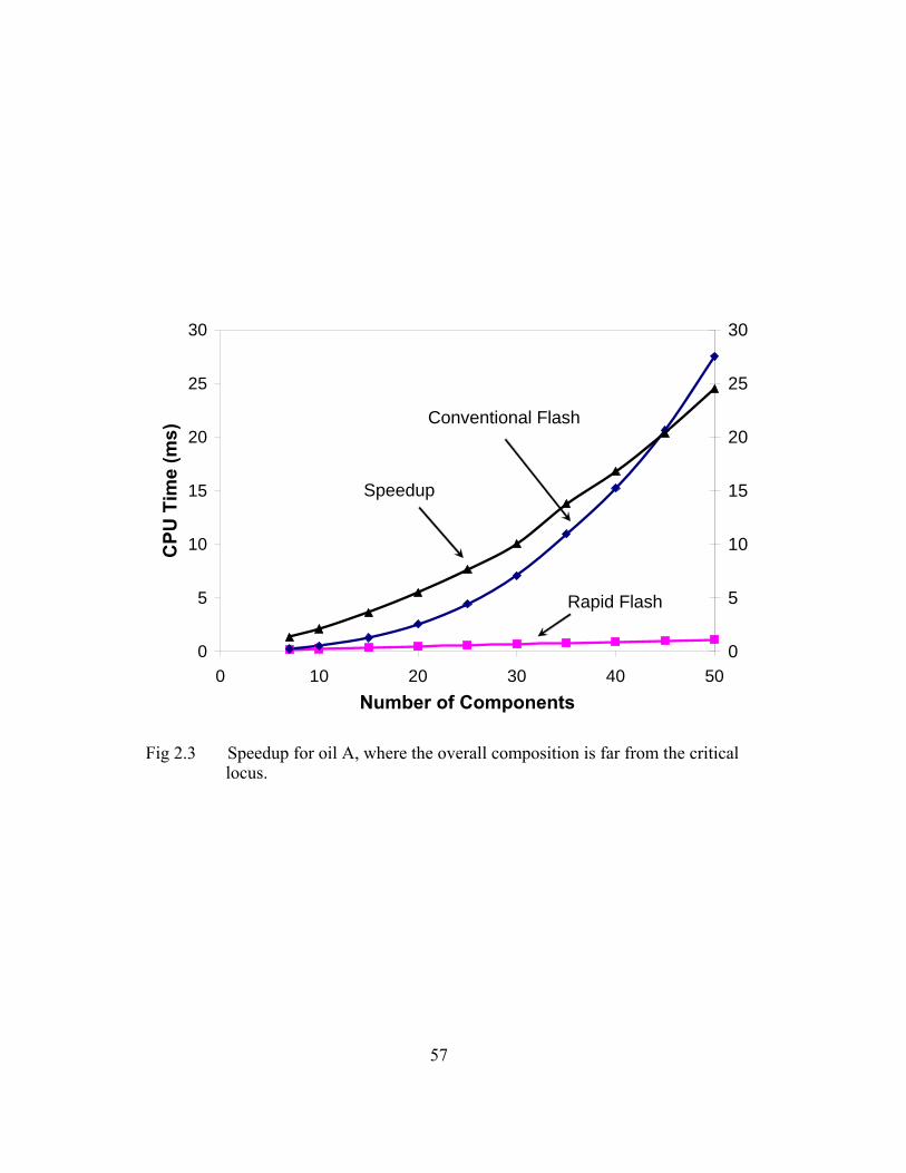
57
0
5
10
15
20
25
30
0 10 20 30 40 50Number of Components
CPU
Tim
e (m
s)
0
5
10
15
20
25
30
Speedup
Rapid Flash
Conventional Flash
Fig 2.3 Speedup for oil A, where the overall composition is far from the critical locus.
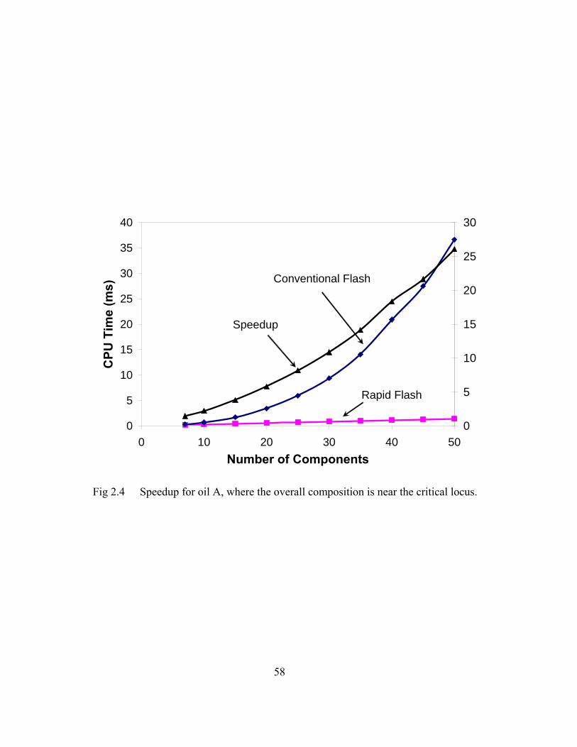
58
0
5
10
15
20
25
30
35
40
0 10 20 30 40 50Number of Components
CPU
Tim
e (m
s)
0
5
10
15
20
25
30
Speedup
Rapid Flash
Conventional Flash
Fig 2.4 Speedup for oil A, where the overall composition is near the critical locus.

59
0
1000
2000
3000
4000
5000
6000
7000
250 300 350 400 450 500 550
Temperautre (F)
Sat
urat
ion
Pre
ssur
e (p
sia)
Original Characterization
Michelsen's Method
Rapid Flash Method
Fig 2.5 Comparison of calculated phase envelopes for gas condensate B (Jutila et al., 2001) to that generated by PVTSIM (Calsep, 2005). The new rapid flash method accurately reproduces the saturation pressures.
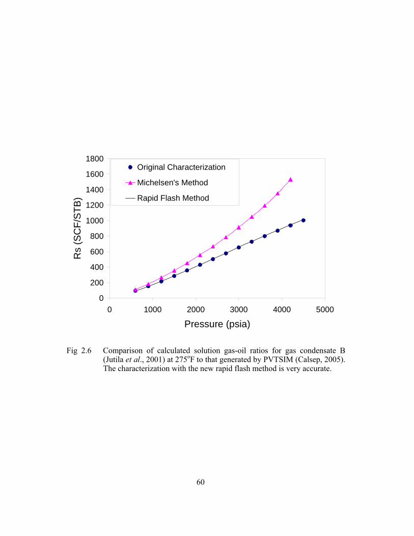
60
0
200
400
600
800
1000
1200
1400
1600
1800
0 1000 2000 3000 4000 5000
Pressure (psia)
Rs
(SC
F/S
TB)
Original Characterization
Michelsen's Method
Rapid Flash Method
Fig 2.6 Comparison of calculated solution gas-oil ratios for gas condensate B (Jutila et al., 2001) at 275oF to that generated by PVTSIM (Calsep, 2005). The characterization with the new rapid flash method is very accurate.

61
1
1.1
1.2
1.3
1.4
1.5
1.6
1.7
1.8
1.9
2
0 1000 2000 3000 4000 5000
Pressure (psia)
Bo
(RB
/STB
)
Original Characterization
Michelsen's Method
Rapid Flash Method
Fig 2.7 Comparison of calculated formation volume factors for gas condensate B (Jutila et al., 2001) at 275oF to that generated by PVTSIM (Calsep, 2005). The characterization with the new rapid flash method is very accurate.

62
0
500
1000
1500
2000
2500
3000
100 300 500 700 900 1100
Temperature (F)
Sat
urat
ion
Pre
ssur
e (p
sia)
OriginalCharacterization
Michelsen's Method
Rapid Flash Method
Fig 2.8 Comparison of calculated phase envelopes for oil C (Hearn and Whitson, 1995) to that generated by PVTSIM (Calsep, 2005). The characterization with the new rapid flash method accurately reproduces the saturation pressures.

63
0
100
200
300
400
500
600
0 500 1000 1500 2000
Pressure (psia)
Rs
(SC
F/S
TB)
Original Characterization
Michelsen's Method
Rapid Flash Method
Fig 2.9 Comparison of calculated solution gas-oil ratios for oil C (Hearn and Whitson, 1995) at 212oF to that generated by PVTSIM (Calsep, 2005). The characterization with the new rapid flash method is very accurate.

64
1
1.05
1.1
1.15
1.2
1.25
1.3
1.35
1.4
1.45
0 500 1000 1500 2000
Pressure (psia)
Bo (R
B/ST
B)
Original Characterization
Michelsen's Method
Rapid Flash Method
Fig 2.10 Comparison of calculated formation volume factors for oil C (Hearn and Whitson, 1995) at 212oF to that generated by PVTSIM (Calsep, 2005). The characterization with the new rapid flash method is very accurate.

65
Chapter 3: Stability Analysis in Reduced Space
In this chapter, stability analysis is done on a single-phase mixture to determine
whether it forms multiple phases or not at a specified temperature and pressure. The
stability analysis calculation is an integral part of the flash calculations. The stability
analysis calculations can be performed for three or more phases simultaneously.
However, this approach may require significant calculations, because the Jacobian matrix
is much larger than that in the two-phase stability analysis calculations. In addition,
two-phase stability tests can be used consequently in this case. For example, for a three-
phase stability analysis, a two-phase flash calculation is first performed, then the phase
stability analysis is applied on each of the pseudo-equilibrium compositions to check
whether each of them is stable or not. It is also important to note that, besides the trivial
solution of i ix z= , one may converge to the trivial pseudo-equilibrium compositions
where i ix y= . A third solution must be found to confirm that the overall composition is
unstable and will form three phases. A three-phase flash calculation is then carried out.
The above procedure is repeated until each phase mixture is stable.
Conventional stability analysis is slow mainly because there are many primary
variables, and the Jacobian matrix is of size C CN N× . In addition, stability analysis
calculations are needed in many grid blocks at a given time. There is a great need for a
much faster and more robust stability analysis calculations.
In this research, we extend the reduced parameters using the proposed BIP model
for an arbitrary number of components and non-zero BIPs matrix. In doing so, the
stability analysis calculations are much faster and should be more robust than
conventional methods.

66
3.1 CONVENTIONAL STABILITY ANALYSIS CALCULATIONS
The objective of stability analysis calculations is to find all stationary points of
the tangent plane distance (TPD) function. In addition, the values of the TPD at these
stationary points need to be evaluated. Consider an CN -component mixture with
overall composition of iz at given reservoir temperature T and pressure P. For a trial
phase composition iy , the TPD can be expressed in dimensionless form as:
( ) ( ) ( )1
1 2
1 2
/
...
...
C
C
C
N
i i ii
N
N
TPD y y y z RT
y y y y
z z z z
μ μ=
= −⎡ ⎤⎣ ⎦
⎡ ⎤= ⎣ ⎦⎡ ⎤= ⎣ ⎦
∑ . (3.1)
where iμ is the chemical potential for component i.
At the stationary points, the partial derivative of the TPD function with respect to
iy is zero. This condition for stationary points can be calculated combined with Gibbs-
Duhem equation using the following:
( ) ( ) ( ) ( ) ( )0C Ci i N N
i
y z y zTPD
y RTμ μ μ μ− − +∂
= =∂
. (3.2)
Equations (3.2) can be re-written as:
( ) ( ) ( ) ( )
C CN Ni i y zy zk
RT RTμ μμ μ −−
= = (3.3)
where k must be constant.

67
Equations (3.3) show that the constant is independent of the component index i.
The chemical potential iμ is further written in terms of fugacity coefficients and
compositions using ( ) ( )/ ln lni i iy RT y yμ φ= + . Noting ( ) ( )/i iz RT d zμ = , Eqs.
(3.3) can be written as:
( ) ( ) ( ) ( )ln lnC CN N
i i i
y zk y y d z
RTμ μ
φ−
= = + − . (3.4)
A new set of primary variables are defined: ki iY y e−= . These new variables are
substituted into Eqs (3.4), yielding:
( ) ( ) 1 2ln ln 0, ...
Ci i i i Ne Y Y d z Y Y Y Yφ ⎡ ⎤= + − = = ⎣ ⎦ . (3.5)
We solve Eqs. (3.5) using Newton-Raphson method with the Jacobian matrix:
ln ln1 1i i i k
ijkj j j j k j
e yJY Y Y Y y Y
φ φ∂ ∂ ∂ ∂= = + = +∂ ∂ ∂ ∂∑ . (3.6)
The derivative ln /i kyφ∂ ∂ is the same as that in conventional phase-split
calculations described in Chapter 2. The remaining partial derivatives can be calculated
using:
2
kj i kk i
ji
i
Y YyY
Y
δ −∂
=∂ ⎛ ⎞
⎜ ⎟⎝ ⎠
∑
∑ . (3.7)

68
When the overall composition is stable, the TPD function must be non-negative at
all stationary points iy . In other words, 0k ≥ is required for all solutions of the above
CN non-linear equations (see Eqs. (3.5)). From ki iY y e−= , we have for a stable phase:
1 1
1C CN N
k ki i
i iY y e e− −
= =
= = ≤∑ ∑ only if 0k ≥ . (3.8)
These non-linear equations (Eqs. (3.5)) can have the following possible solutions:
1
1
trivial solution
1
1 with
C
C
i iN
ii
N
i i ii
Y z
Y
Y Y z
=
=
=
>
≤ ≠
∑
∑
. (3.9)
If all the roots to Eqs. (3.5) yield 1
1CN
ii
Y=
≤∑ , the overall composition is stable, and
the mixture will maintain a single phase; otherwise that phase must split in two phases.
However, it would be costly to calculate all these roots without knowing a priori how
many roots exist. Michelsen (1982a) suggested that it is often efficient enough to only
test the initial guesses using compositions made up of either purely the most or the least
volatile component in the mixture rather than test all the possible initial guesses. This
approach is much easier and faster, and in most cases yields satisfactory results.
Nevertheless, stability analysis calculations using the conventional approach require
solving for stationary points using NC variables.

69
3.2 STABILITY ANALYSIS CALCULATIONS IN REDUCED SPACE
Stability analysis can also be performed in reduced space where the number of the
primary variables required to iterate on is much less. As a result, stability analysis
calculations in reduced space have significant speedup compared with the conventional
method. Further, the determination of stationary points of the TPD is more robust in
reduced space since the global minimum of the TPD in theory should be easier to find.
As shown in the phase split calculation (see Chapter 2), the fugacity coefficients
are only functions of the reduced parameters, so that:
( ) ( )ln lni i iY d z φ= − Θ , or ( )( ) ( )exp /i i iY d z φ= Θ . (3.10)
From 1 1 1
1C C CN N N
k ki i i
i i i
y Y e e Y= = =
= = =∑ ∑ ∑ , we have:
1/
CN
i i ii
y Y Y=
= ∑ . (3.11)
Hoteit and Firoozabadi (2006) derived the objective function for the reduced
method using dominant eigenvalue decomposition (Hendriks, 1988). From the definition
of reduced parameters in Chapter 2, we have:
1 1 10 for 1,...,5
C C CN N N
j i ji j i ji ii i i
y q Y q Y j= = =
= Θ − = Θ − =∑ ∑ ∑ . (3.12)
If 1
CN
ii
Y=∑ is multiplied on both sides of Eqs (3.12), the following are obtained:

70
( )1 1 1
0C C CN N N
j i i ji i j jii i i
Y Y q Y q= = =
= Θ − = Θ −∑ ∑ ∑ . (3.13)
Substitution of Eqs (3.10) into Eqs (3.13), denoting ( )( )exp id z as ( )iD z ,
yields the objective functions using reduced parameters as:
( )
1
0 for 1,...,5CN
i ik ki
k k
q DF k
φ=
Θ −= = =∑ . (3.14)
The Jacobian matrix for the objective functions in Eqs. (3.14) is evaluated as:
( )
21
/CNij i ik k ji
ij kkj k
qFJ Dδ φ
φ=
− Θ − ∂ ∂Θ∂= =∂Θ ∑ . (3.15)
The derivatives of the fugacity coefficients with respect to the reduced parameters
are exactly the same as that in Chapter 2 for the phase-split calculations. In addition,
each of the reduced parameters must fall into a hyperspace bounded by min maxi i iq q≤ Θ ≤ ,
where min max and i iq q are the smallest and largest values of the reduced parameter for all
pure components. The procedure for stability analysis is as follows:
1. Evaluate the reduced parameters for the overall composition, and calculate
the fugacity coefficients of the overall composition. Calculate the values
of ( )i i iD z zφ= , which are constant throughout the stability analysis;
2. Make an initial guess of the reduced parameters Θ for the trial phase. A
possible approach is to use Θ that come from either the most or least
volatile components, and use both initial guesses to initialize the NR
iteration, as suggested by Michelsen (1982a). Another popular approach

71
uses the initial guesses of j ji i ii
q K zΘ =∑ and /j ji i ii
q z KΘ =∑ , where
the K-values come from Wilson correlations (1969). This dissertation
uses the latter approach;
3. Calculate cubic EOS parameters (e.g. ma and mb ). This step is very
straightforward and depends on the selected EOS and its associated
mixing rules. The cubic EOS for Z-factors is then solved for the trial
phase. This step requires determining the roots of the cubic EOS for each
phase using a cubic solver. The correct root is the one that gives the
lowest Gibbs energy;
4. Calculate the fugacities of each component in the trial phase. The selected
cubic EOS is used to determine an expression for the fugacity;
5. Check to see if convergence criteria are met. In this research, a tolerance
of the objective function in Eqs. (3.14) of 10-10 is used;
6. Update the reduced parameters by Newton-Raphson iteration (for faster
convergence) if the criteria of Step 5 have not been satisfied;
7. Evaluate iY by substitution of the converged solution of reduced
variables into Eqs. (3.10);
8. If the NR iteration converges to a trivial solution or non-trivial solution
where 1
1CN
ii
Y=
≤∑ , the other initial guess is used and steps 3-7 repeated. If
the NR iterations converge to a non-trivial solution that gives 1
1CN
ii
Y=
>∑ ,
the phase-split calculations (see Chapter 2) can be performed immediately
because the overall composition is unstable and forms two or more phases.

72
3.3 EXAMPLE CALCULATIONS
This section presents several example stability calculations with various fluid
characterizations using the new reduced method to examine the efficiency of stability
analysis calculations. The results are compared with the conventional method that
iterates on iY . This section shows the advantages of the reduced method over the
conventional method especially in speed.
3.3.1 IMPROVED SPEED
The most important advantages using reduced parameters over the conventional
methods are significantly improved speed. We uses different oils at various
temperatures and pressures to show: (1) how fast the stability analysis calculations are
when the reduced method is compared with the conventional method; and (2) how fast
the stability analysis calculations are compared with the phase-split calculations of the
reduced method.
3.3.1.1 STABILITY ANALYSIS FOR OIL A FAR FROM CRITICAL POINT
First, we examine the synthetic seven-component oil A described in Section
(2.5.1) at 260oF and 300 psia. The computation time required for the stability analysis in
the conventional method is determined. With the same initial guess of the trial phase
compositions, the stability analysis calculations are performed in reduced space using the
procedure outlined earlier. Even though the objective functions are different in these
two methods, the final converged compositions are within an absolute tolerance of 10-10
in the composition to ensure that the same convergence criteria were met (Okuno, 2007).

73
Figure (3.1) compares the computation time required for convergence for both
methods with a different number of pseudocomponents. Additional pseudocomponents
are obtained by the same method detailed earlier (see Section (2.5.1)) that splits the least
volatile component to a desired number of pseudocomponents. For the case studied, the
computational time with the new method is about 1.9 times faster at seven components,
and 23 times faster at thirty-five components than the conventional method. It is also
shown that the stability analysis calculation using thirty-five components has a similar
speed as that with ten components in the conventional method. Figure (3.2) shows the
comparison of computation time per NR step. Stability analysis calculations using the
reduced parameters are even faster per NR step, because less primary variables are
required compared with the conventional stability analysis.
In addition, compared with Fig. (2.3), Fig. (3.1) also shows that the speedup in the
stability analysis calculations is greater than that in the split calculation. This is mainly
because: (1) the number of primary variables in the conventional method is the same in
both subroutines ( CN ); however, in the reduced method, the stability analysis requires
five primary variables while the phase-spit calculation requires six; (2) the stability
analysis in reduced space requires fewer iterations than phase-spit calculations in this
study, which increases speedup.
The speedup in stability analysis calculations increases significantly with the
number of components, as expected. The computation time for the reduced method
approximately increases linearly only with the number of pseducomponents, whereas the
conventional method increases on the order of 2.7. The following may explain why the
reduced method is almost linearly dependent on the number of pseudocomponents while
the conventional method increases at the power of 2.7:

74
1. In the reduced method, a five by five Jacobian matrix is used regardless of
the number of pseudocomponents. The difference in computation time is
mainly controlled by the evaluation of the objective functions and the
Jacobian matrix. The evaluation is almost linearly correlated to the
number of pseudocomponents;
2. In the conventional method, the speed of Gaussian elimination depends on
approximately the third power of the number of pseudocomponents, the
evaluation of Jacobian matrix approximately the second power, and the
evaluation of the objective function is approximately linearly correlated to
the number of pseducomponents. Normally, the Jacobian evaluation
takes the largest portion of the computation time, followed by Gaussian
elimination. The evaluation of the objective function is the least
expensive. Therefore, in the conventional method, the computation time
increases between the second and third power as a function of the number
of pseudocomponents.
3.3.1.2 STABILITY ANALYSIS FOR OIL A NEAR CRITICAL POINT
Oil A is again examined at 485oF and 1044 psia to illustrate the calculation near
the critical points. The speed of the reduced method is compared with that of the
conventional method. The total CPU time is plotted in Figs. (3.5) and (3.6).
Both reduced and conventional methods slow down stability analysis calculations
near the critical point. The reduced method is over two times faster than the
conventional method when seven components are used, compared to approximately 1.9
far from the critical locus. Similar results were obtained in the phase-split calculations.

75
That is, the reduced method has a larger speedup near the critical point than far from the
critical point.
3.3.1.3 SPEED COMPARISON FOR STABILITY ANALYSIS AND PHASE-SPLIT CALCULATIONS
It is also of interest to compare the total computation time of stability analysis and
phase-split calculations, to determine that whether stability analysis should be used or
not. Many simulators apply stability analysis calculations before using phase-split
calculations. This is to avoid the slow phase split calculations when the phase in the
grid block in the previous time step is stable. This section compares the computation
time of both stability analysis and phase-split calculations using the reduced method.
For the same oil A, the comparison of both calculations using the reduced method
is shown in Fig. (3.3). In this figure, we did not use successive substitution in the phase-
split calculations, which is different from the procedure in Chapter 2. Figure (3.3)
indicates a mixed result. The stability analysis calculation is faster than the phase split
calculation using the reduced method, by a factor approximately 2.5. This is mainly
because the number of iterations required for the stability analysis calculation (three NR
iterations) is significantly less than that for the phase-split calculations (seven NR
iterations). In each NR step, the stability analysis calculation is only moderately faster
than the phase-split calculation, as shown in Fig. (3.4). The reduction in speedup is
mainly because the Jacobian matrix is smaller (six compared with five). Similar results
were seen by Hoteit and Firoozabadi (2006).
The fact that stability analysis is substantially faster than phase-split calculations
should be examined for more fluids. In the example calculations, the non-trivial
solution is always found with the first initial guess of i i iY K z= . Stability analysis

76
calculations will slow down if a second initial guess is required. When both initial
guesses are required, the CPU time for the phase-spit calculations is approximately 50%
more than that for the stability analysis calculations. This is still a substantial savings of
time if most of the grid blocks are in single phase. When a gas flood is operated at a low
pressure, most grid blocks have two phases where the application of stability analysis
may have little advantage.
3.3.2 IMPROVED ROBUSTNESS OF REDUCED METHOD
Previous research has shown that robustness in stability analysis is improved in
reduced space mainly because of a smoother Gibbs free energy surface in the reduced
space (Firoozabadi and Pan, 2002). In this research, we did not found a case where the
conventional method failed to converge. This is because in stability analysis, there is
always at least one solution, that is the trivial solution of i iy z= . In addition, because
the Rachford-Rice or a similar method is not used in the stability analysis, there is no
convergence problem owing to the iterative RR procedure. However, we did find that
stability analysis in reduced space is relatively faster compared with the conventional
method, especially when the overall composition is near a critical point. We compare
the speedup in Figs. (3.1) and (3.5), and find out that the speedup in Fig. (3.5) is
significantly greater than that in Fig. (3.1). This is mainly because the conventional
method is relatively slower to converge. Because of the improved smoothness in
reduced space, there is not much of a difference in convergence in both cases.
Nevertheless, the reduced method converges significantly faster than the conventional
method even when the overall composition is near critical. With fewer primary
variables, we speculate that the reduced method should be more robust.

77
3.4 CONCLUSIONS
In this chapter, the reduced method was implemented to perform stability analysis
calculations for two phases. Calculations based on direct solution of the tangent plane
distance function were formulated. The example cases studied reveal the advantages of
the new method over the conventional method as the following:
1. The number of primary variables in the direct solution of the TPD function
is significantly reduced from NC to a maximum of five, depending on
binary interaction parameters;
2. The computation speed is significantly enhanced compared to the
conventional method without sacrificing accuracy. The conventional
method requires approximately 1.9 times the computation time than for
the reduced method at seven components, and 23 times at 35 components;
3. The robustness of the rapid calculations is also slightly improved for
compositions near the critical locus;
4. Compared to phase-split calculations in reduced space, stability analysis
calculations in reduced space are faster by approximately 3 times
independent of the number of components. However, if most of the grid
blocks are two phases at the previous time step, it may not be efficient to
apply the stability analysis calculations at all. Negative flash calculations
with the reduced method may be all that is required.

78
0
2
4
6
8
0 10 20 30 40
Number of Components
CPU
Tim
e fo
r SA
(ms)
0
5
10
15
20
25
Spee
dup
Rat
io
Speedup
Reduced Method
Conventional Method
Fig. 3.1 Comparison of the total computation time for both the reduced method and the conventional method in stability analysis as a function of the number of pseudocomponents for oil A. For seven components, the speedup from the conventional method is approximately 1.9 and for 35 components, the speedup is 23 (Okuno, 2007).

79
0
0.5
1
1.5
2
0 10 20 30 40
Number of Components
CPU
Tim
e fo
r SA
(ms)
0
5
10
15
20
25
30
Spee
dup
Rat
io
Speedup
Reduced Method
Conventional Method
Fig. 3.2 Comparison of the computation time for stability analysis per NR iteration for oil A that is far from a critical point. Both the reduced and the conventional methods are tested. As shown, the reduced method is significantly faster (Okuno, 2007).

80
0
0.2
0.4
0.6
0.8
1
0 10 20 30 40
Number of compositions
CPU
Tim
e (m
s)
Split Calculation
Stability Analysis
Fig. 3.3 Comparison of the total computation time for stability analysis and phase-split calculations using the reduced method for oil A. The stability analysis is approximately three times faster. In this case, the oil is far from a critical point (Okuno, 2007).

81
0
0.05
0.1
0.15
0 10 20 30 40
Number of compositions
CPU
Tim
e pe
r Ite
ratio
n (m
s)
Split Calculation
Stability Analysis
Fig. 3.4 Comparison of the computation time per iteration for stability analysis and phase-split calculations using the reduced method for oil A. The stability analysis in reduced space is moderately faster than the phase-split calculation in reduced space. In this case, the oil is far from a critical point (Okuno, 2007).

82
0
10
20
30
40
50
0 10 20 30 40
Number of Components
CPU
Tim
e fo
r SA
(ms)
0
5
10
15
20
25
30
35
40
Spee
dup
Rat
io
Speedup
Reduced Method
Conventional Method
Fig. 3.5 Comparison of the total computation time for oil A near a critical point. Both the reduced and the conventional methods are used. The reduced method is much faster than the conventional one (Okuno, 2007).

83
0
1
2
3
4
5
0 10 20 30 40
Number of Components
CPU
Tim
e pe
r Ite
ratio
n (m
s)
0
5
10
15
20
25
30
35
Spee
dup
Rat
io
Speedup
Reduced Method
Conventional Method
Fig. 3.6 Comparison of the computation time for stability analysis per NR iteration for oil A near a critical point. The reduced method is significantly faster and requires fewer iterations (Okuno, 2007).

84
Chapter 4: Two-Phase Flash Calculations with Constant K-values
Rachford-Rice (1952) iterations are widely used in equations-of-state (EOS) flash
calculations to determine phase equilibrium compositions with constant equilibrium
ratios (K-values). The method, however, can be slow to converge and in some cases
may not converge at all.
In this chapter, we derive a new objective function in terms of one of the
equilibrium liquid phase mole fractions. The new method also specifies a small window
in which the physical roots must lie. The new objective function is continuous and
nearly linear in this predetermined window. We first summarize conventional Rachford-
Rice (1952) calculations, and then derive the new objective function and window.
Several example calculations are performed and the results are compared with the
Rachford-Rice (1952), Wang and Orr (1997, 1998), and Leibovici and Neoschil (1992)
methods. The Peng-Robinson (1977, 1978) EOS is also used to demonstrate that the
function can converge very near the critical region.
4.1 RACHFORD-RICE FLASH CALCULATIONS
Rachford-Rice (1952) iterations are typically used to determine the phase
compositions and amounts as outlined in step 3 in Section (2.1). The objective function
for this method is easily derived from the definition of K-values for two-phase
equilibrium:
1,...,i i i Cy K x i N= = . (4.1)

85
where iy and ix are equilibrium compositions of the vapor and liquid phase
respectively, iK are the constant equilibrium ratios and CN is the number of
components. Furthermore, a mass balance on a given component gives,
1,...,i i i Cz Lx Vy i N= + = (4.2)
where L is the molar fraction of the liquid phase, V is the molar fraction of the vapor
phase, and iz is the overall composition of the mixture. The phase compositions and
amounts must sum to 1.0. Substitution of Eqs. (4.1) into Eqs. (4.2) together
with 1L V+ = gives,
( ) 1,...,
1 1i
i Ci
zx i NV K
= =+ −
. (4.3)
The Rachford-Rice (1952) objective function is then defined by,
( ) ( )( )1 1 1
10
1 1C C CN N N
i ii i
i i i i
z KF V y x
V K= = =
−= − = =
+ −∑ ∑ ∑ . (4.4)
The roots of Eq. (4.4) in terms of the vapor molar fraction are often solved by
Newton-Raphson method. Convergence is achieved once the updated value of V
satisfies a relative tolerance of say 10-8. Once V is determined, the equilibrium phase
compositions are calculated from Eqs. (4.3) and (4.1).
Unfortunately, there are 1CN + roots for V given by Eqs. (4.3) and the function
can be highly nonlinear owing to CN poles at 1/(1 )iV K= − . Rachford and Rice
(1952) initially constrained the value of V to lie within the range or window from [0, 1],

86
but this requires that the overall composition lies within the two-phase region of the
current set of K-values. Whitson and Michelsen (1989) improved the robustness for
overall compositions outside the two-phase region (negative flash calculations) by
showing that the correct root of V can be defined from the poles corresponding to the
largest and smallest volatile components, that is, within the window
11/(1 ) 1/(1 )CNK V K− < < − . Even with this improvement, the Rachford-Rice (1952)
function still suffers from the disadvantages described previously, and may not always
converge for some special cases.
4.2 DERIVATION OF NEW METHOD
Similar to the approach of Whitson and Michelsen (1989), the derivation of our
new objective function and window requires that the components are ordered based on K-values. We assume that 1 1
CNK K> > .
The objective function is determined by transforming the original compositions so
that equilibrium phase compositions of the intermediate components in the transformed
compositional space are equal. For a ternary system this directly implies that all tie lines
are parallel, including the limiting tie lines at critical points. Such a transform reduces
the nonlinearity of the objective function.
The transform follows closely the procedure described by Hand (1930) for ternary
diagrams, although he used transformation parameters independent of composition. We
extend that approach here to a multicomponent system by introducing a set of
transformation parameters, in which each one is a function of composition. The
transformed intermediate compositions are given by

87
( ) ( )
( )
* *
1 1
*
1
1 1 1 1
for 2,..., 11 1
i ii i
i i
ii C
i
x yx yx y
zz i Nz
α α
α
= = = =− + − +
= = −− +
(4.5)
where iα is the transformation parameter. From Eq. (4.5), iα can be evaluated by
1 1
111 2,..., 1ii C
i
K i Nx K Kα⎛ ⎞⎜ ⎟⎜ ⎟⎝ ⎠
−= + = −−
. (4.6)
From Eqs (4.5) and (4.6), one can also show that for the liquid phase:
( )
( ) ( )1 1
1 1 1
1 2,..., 1
1i
i Ci i
K z xx i N
K z K K x−
= = −− + −
. (4.7)
Equations (4.7) can also be derived directly from Eqs. (4.3) by solving for V, but
with loss of physical meaning. In addition to Eqs. (4.7), the phase compositions must
sum to 1.0 so that
1
11
C
C
N
iNi
x x−
== − ∑ (4.8)
1
11
C
C
N
iNi
y y−
== − ∑ . (4.9)
If we substitute Eqs (4.8) and (4.3) into Eq (4.9), we have after some
rearrangement:

88
( )( )
( )( )
111
21 0
1 1
CC C
C C
N iN Ni
iN N
K K K Kx x
K K
−
=
− −+ + =
− −∑ . (4.10)
Substitution of Eqs (4.7) into Eq (4.10) gives the new objective function as,
( )
( )( )
( )( ) ( )
11 1
11 1
2 1 1 1
11
1 0
11
C
C
CC
C
N
N
N i N i
i i iN
K KF x x
K
K K z K xK z K K xK
−
=
⎛ ⎞⎜ ⎟⎜ ⎟⎝ ⎠
⎡ ⎤⎢ ⎥⎢ ⎥⎣ ⎦
−= + +
−
− −=
− + −−∑
. (4.12)
In addition, the derivative for NR iteration is given by:
( )( )( )
( ) ( ) ( )
11 11
221 1 1 1
1 1
1 1 1
CCC
C C
Ni N i iN
iN N i i
K K K K z zK KdFdx K K K z K K x
−
=
− − −−= +
− − − + −⎡ ⎤⎣ ⎦∑
The correct root(s) from the new objective function must lie within a small
window. This window is developed by limiting all phase and overall compositions to be
positive in Eqs. (4.7). The simplest expression for the window (although not the
smallest possible) is given by
1 11 1
1 1C C
C C
N N
N N
K Kz xK K K K
⎛ ⎞⎜ ⎟⎜ ⎟⎝ ⎠
− −≤ ≤
− − . (4.13)
The derivation of Eq. (4.13) along with a more complex, but even smaller window
for 1x can be found from Eqs (4.16) and (4.18) in Section (4.2.1). Because of its

89
simplicity, we only use Eq. (4.13) in the calculations made in this research. When at
least one composition is negative, a new window is derived in Appendix.
The new objective function of Eq. (4.12) always converges to a physical root no
matter the overall composition. The new method has significant advantages over the
Rachford-Rice (1952; Whitson and Michelsen, 1989) or similar variations (Wang and
Orr, 1997, 1998). First, 1 0x = is not a trivial root of the new objective function as it is
for Wang and Orr (1997, 1998). Second, when multiple tie lines exist that go through
the same composition, the new function can find all tie lines or physical roots from the
negative flash. Third, the root(s) must lie within a very small window as defined by Eq.
(4.13). Fourth, the function is often linear and continuous within that window. There
are never poles within the window, as proved in Section (4.2.2). Fifth, the function is
always positive at the lower limit of the window and negative at the upper limit so that
bisection methods can be easily used if required (see Section (4.2.3.)). Last, the new
objective function is properly scaled to reduce truncation error compared with that of
Rachford-Rice (1952). These features can significantly reduce the number of iterations
for convergence compared with Rachford-Rice (1952) and are discussed in the next
section.
4.2.1 Initial Guess for Phase Mole Composition
A good initial guess for the equilibrium liquid phase mole fraction is important
for convergence. In the derivations that follow we assume that all overall compositions
are positive.
From Eq. (4.3), we have

90
( )1= for 1, ,11
i i i iC
ii i
z x x zV i NKK x− −= =
−−… . (4.14)
Considering only the lightest and heaviest components, Eq. (4.14) is
( )1 1
1 1
1 11 11
C C
C C
N N
N N
z xz xV K KK x−−
= = ≤− −−
(4.15)
because / 0
C CN Nz x ≥ . Thus, after rearrangement of Eq. (4.15), we obtain the left-hand
side of Eq. (4.13) to be
11min1
1C
C
N
N
Kx zK K
⎛ ⎞⎜ ⎟⎜ ⎟⎝ ⎠
−=
− . (4.16)
To determine a maximum limit, we recognize that for all components
Ci i iNK x K x≥ . Summation of this expression yields after some rearrangement:
( )1 1 1 12 2
1 1 1C C
C C
N N
i i iN Ni i
K x y K x K x K x= =
= − = − ≥ = −∑ ∑ . (4.17)
From Eq. (4.17), we obtain the right-hand side of Eq. (4.13) as,
1max1
1C
C
N
N
Kx
K K−
=−
. (4.18)
A more complex, but smaller window can be found recognizing that all
equilibrium liquid phase compositions must be positive so that

91
10 if 1
0 1 if 1
i ii
i i
x KKx K
≤ ≤ >
≤ ≤ < . (4.19)
Substitution of Eqs. (4.7) into Eqs. (4.16) and (4.18) gives,
( )
( ) ( )1
1min1 1
1max for all 1
1i
ii i
K zx K
K K z K
⎡ ⎤⎢ ⎥⎢ ⎥⎣ ⎦
−= <
− − − (4.20)
( )
( ) ( )1
1max11 1
11min , for all 1
1C
C
Nii
Ni i i
KK zx KK KK z K K K
⎡ ⎤⎢ ⎥⎢ ⎥⎣ ⎦
−−= >
−− − −. (4.21)
This smaller window compared with Eq. (4.13) can decrease the number of
iterations slightly, especially when the number of components is greater than 10. For
example, when 12CN = the smaller window is approximately 15% faster in
computational time than when using the window given by Eq. (4.13). Equation (4.20) is
identical to that used by Lebovici and Neoshil (1992), but the maximum limit given by
Eq. (4.21) is new to this research.
The window given by Eqs. (4.20) and (4.21) can also be used to determine if a
physical root exists. If 1max1min 0x x= = then no physical root exists. For reservoir
simulation, however, this problem will not arise, but it might in other applications such as
the MMP/MME determination from analytical methods (Jessen et al., 1998; Yuan and
Johns, 2005).

92
4.2.2 Continuity of New Method
The objective function contains no poles within the window of Eq. (4.13). The
poles of Eq. (4.12) are defined by
( )( )
11
1
1, 2,..., 1i
Ci
K zx i N
K K−
= = −−
. (4.22)
Because ( )( ) ( )( )1 11 1
C Ci iN NK K K K K K− − < − − ,
( )( )
( )( )
111min
1 1
11 C
C
Ni
i N
K zK zx
K K K K
−−< =
− − . (4.23)
Equation (4.23) shows that when 1 0z ≠ , all poles are to the left (towards negative
1x ) of the window given by Eq. (4.13). Thus, the objective function will be continuous
in the window. When 1 0z = the pole coincides with 1minx and there is a discontinuity
in the objective function at 1minx . As explained in Section (4.2.3) that discontinuity can
be easily handled by selecting another variable to iterate on.
4.2.3 Finding All Possible Roots
More than one physical root is possible when one or more components are not
present, for example at the apex or the base of a ternary diagram. It may also be
possible with the new method that no root exists within the window when the lightest
component is not present in the overall composition and 0V > . For some applications
such as MMP/MME estimation (Jessen et al., 1998; Yuan and Johns, 2005), we want to
find all tie lines that extend through the overall composition. An easy method to find all

93
tie lines is first to make the flash calculation with all CN components. The flash is then
repeated, but the number of components is reduced one by one by eliminating the missing
component(s) from the objective function. This would continue until all components
have K-values less than 1.0. Each flash will yield another tie-line solution.
A more formal way of writing this is to recognize that the selection of the
component to calculate the liquid phase mole fraction is arbitrary. Thus, we can write
Eq. (4.12) in a more general form as:
( ) ( )( )
( )( ) ( )1, ,
11 0
1 1 1
C refref
ref ref
Ni j jij
j ji i j i ref i j j i j
z K xK KK KF x x
K K K z K K x= ≠ ≠
⎛ ⎞⎜ ⎟⎜ ⎟⎝ ⎠
−−−= + + =
− − + −− ∑ . (4.24)
where jK is the selected component to use as the iteration variable and 1jK > and
1refK < . Typically,CNrefK K= and j iK K= .
The case when no root exists within the window can be identified prior to
calculation. When 1 0z = , no root is present when
1
1
21 01
CC
C
NN
ii N
K KzK
−
=
⎛ ⎞⎜ ⎟⎜ ⎟⎝ ⎠
−+ <
−∑ . (4.25)
Equation (4.25) is derived by finding when the objective function given by Eq.
(4.12) is negative at (0 )F + . For such cases there is a discontinuity at 1 0x = .
Another possible complication for the new method and the Rachford-Rice (1952)
is when the overall composition of the primary variable is very small, that is, 91 10z −< .
In such cases many iterations are often required to obtain convergence because of the
nonlinearity that occurs near the root. This problem is more likely to occur with
Rachford-Rice. For the new method, we can eliminate this problem by changing the

94
primary variable to the next lightest component. Based on experience we recommend to
do this when 121 1/ 10z K −≤ . The variable to iterate with should be chosen so that
12/ 10i iz K −≥ when 1iK > or 1210i iz K −≥ for 1iK < .
4.3 EXAMPLE CALCULATIONS
This section presents several example calculations using the new method. The
robustness and speed with the new objective function are compared with that obtained
with the iterative methods of Rachford-Rice (1952; Whitson and Michelsen, 1989), Wang
and Orr (1997, 1998), and Leibovici and Neoschil (1992). To ensure a proper
comparison, the convergence criteria for each method is always 10-8 for the relative error
in V. For methods that iterate on 1x , we translated the value of 1x to V so that the
criteria for all methods were exactly the same.
4.3.1 Improved Robustness and Linearity of New Method.
We first consider a ternary system with constant K-values, where 1 5.0K = ,
2 2.0K = and 3 0.5K = . Figure (4.1) shows the phase behavior for this set of K-values
along with the overall compositions at points A, B, C, and D, all of which lie on the same
tie line or its extension. We then examine convergence for phase behavior with K-
values near 1.0 and also with a cubic EOS (Peng and Robinson, 1977, 1978).
4.3.1.1 Point A
This composition lies near the center of the two-phase region in Fig. (4.1).
Figure (4.2) shows the Rachford-Rice (1952) objective function for this tie line along
with the correct root (solution) that lies within the window given by Whitson and

95
Michelsen (1989). Figure (4.3) also shows a comparison of the objective functions of
Wang and Orr (1997, 1998) and our new function plotted against the same parameter 1x .
The window based on Eq. (4.13) is also shown in Fig. (4.3).
Because point A lies within the two-phase region all methods can converge to the
same root. Wang and Orr’s method (1997, 1998), which does not specify a window
other than 10.0 1.0x≤ ≤ , could converge, however, to the trivial solution at 1 0x =
depending on the initial guess. That trivial solution does not exist in our proposed
objective function. The new function is also more linear than either Rachford-Rice
(1952) or Wang and Orr (1997, 1998) so that fewer iterations are required for
convergence. As shown in Fig. (4.4), the number of iterations using the new function is
largely independent of the initial guess within the window of Eq. (4.13). For example,
for an initial guess of V of about 2.0, Rachford-Rice (1952; Whitson and Michelsen,
1989) takes 12 iterations to converge compared with only 5 iterations for the new
function. Both methods require about 4 iterations when the initial guess is closer to the
actual root, although with the new function there is a small region very near the correct
root of 1x where three iterations are required compared with four in Rachford-Rice
(1952). For the same initial guess, the number of iterations with the new function will
always be less than or equal to the number of iterations with Rachford-Rice (1952).
4.3.1.2 Point B
Composition B is in the single phase region and lies on the same tie-line extension
as A, but unlike A does not contain component 1. Thus, there is a second tie-line that
extends though A along the base (2-3 axis) of the ternary diagram. Ideally, a negative
flash at this composition could yield the root corresponding to either tie line.

96
Point B is problematic for both Rachford-Rice (1952) and Wang and Orr (1997,
1998). The Wang and Orr objective function (1997, 1998) cannot be calculated because
1z is zero there and a divide by zero error occurs. The Rachford-Rice (1952) function
(see Fig. (4.5)) does have the root corresponding to the tie line in the base of the ternary
diagram, but this root is outside of the Whitson-Michelsen window (1989). Thus, the
Rachford-Rice (1952) root is not bounded correctly and convergence is not guaranteed.
The window for the new function (see Fig. (4.6)), however, contains the correct
root for the tie line that passes through point A. Furthermore, Section (4.2.3) describes
an easy way to locate the second tie line in the base of the ternary diagram. Thus, both
tie lines can be found with the new function with few iterations. The new function can
also converge even when the overall composition is on any one of the three apexes of the
ternary diagram.
4.3.1.3 Point C.
This overall composition is in the vapor region, but also lies on the tie-line
extension through point A. Thus, like B this is a negative flash. Figure (4.7) gives the
Rachford-Rice function (1952), whereas Fig. (4.8) compares the Wang and Orr function
(1997, 1998) with our new function. Similar to point A, all methods converge to the
correct solution, although the number of iterations with Rachford-Rice (1952) is similar
to that shown previously in Fig. (4.4). Also, as for point A, the Wang and Orr function
(1997, 1998) can converge to the trivial root depending on the initial guess.

97
4.3.1.4 Point D.
Composition D lies exactly on the 1-2 axis of the ternary diagram. This point is
again problematic for Rachford-Rice (1952) as the correct root corresponding to the tie-
line extension through point A is not present (see Fig. (4.9)). The root shown in Fig.
(4.9) for Rachford-Rice (1952) corresponds to a tie line that is nonphysical, that is, one or
more of the equilibrium phase compositions are negative. Wang and Orr’s objective
function (1997, 1998) also cannot converge to the correct root as only the trivial solution
( 1 0x = ) is present (see Fig. (4.10)). The new method, however, has the correct root and
will converge in a few iterations.
4.3.1.5 Point E - Near Critical
The new method also converges well for points very near the critical locus where
all K-values are within numerical precision of 1.0. For example, Figure (4.11) shows the
tiny two-phase region for K-values of 1 1 2K ε= + , 2 1K ε= + and 3 1K ε= − with
910ε −= . In that plot the bubble-point curve and dew-point curve nearly coincide with
each other.
All methods converge to the correct root; although the Wang and Orr method
could mistakenly converge to the trivial root at 1 0x = (see Figs. (4.12) and (4.13)).
Similar to convergence at point A, the new function requires fewer iterations for
convergence than Rachford-Rice (1952).
For very small values of ε , the Rachford-Rice method (1952) can also suffer
from truncation error owing to addition or subtraction of a large number from a small
one. The new function, which is better scaled, preserves all sixteen digit accuracy if
double precision is used, whereas Rachford-Rice (1952) has thirteen digit accuracy. The
scaling issue is apparent by considering the values of the objective functions. For

98
example, for an initial guess at the midpoint of Whitson-Michelsen window (1989), the
value of the Rachford-Rice objective function (1952) is 102.35 10−− × , and its derivative
is 181.59 10−− × , much small than the value of the objective function. The value of the
new objective function at the midpoint of Eq. (4.13) is 0.076, and its derivative is -3.76.
4.3.1.6 Use of New Method with Equations of State
Michelsen (1993) showed that successive substitution for updating K-values is
guaranteed to converge, although very slowly near critical points (convergence could be a
trivial solution, however). Figure (4.14) shows a three-component phase behavior
predicted using the Peng-Robinson (1977, 1978) EOS and our new function.
Convergence in the flash calculations is always achieved as the critical point is
approached to within the tolerance used for component fugacities. The advantages of
the new function are twofold: (1) the number of iterations are generally reduced
decreasing the time for the flash calculations near the critical point; and (2) convergence
is slightly more accurate near the critical point than when Rachford-Rice (1952) is used.
4.3.2 Improved Speed of New Method.
There are two ways to examine the speedup of the new method compared with
Rachford-Rice (1952; Whitson and Michelsen, 1989) and Leibovici and Neoschil (1992).
The first approach is to perform compositional simulations and compare the average
processor time. That approach is useful because it incorporates prior values as the initial
guess for the next time step, but simulation may not cover all possible combinations of K-
values and overall compositions. Another approach is to randomly vary the
compositions and K-values within a realistic range to estimate the average overall
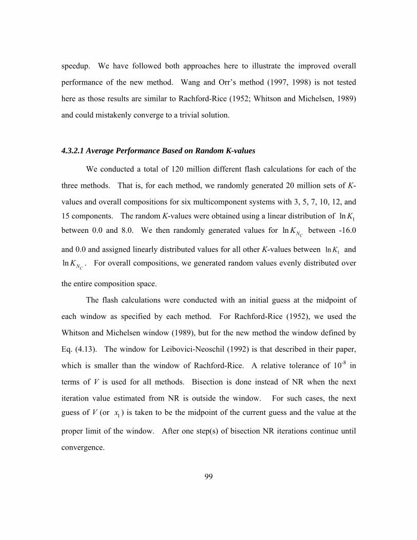
99
speedup. We have followed both approaches here to illustrate the improved overall
performance of the new method. Wang and Orr’s method (1997, 1998) is not tested
here as those results are similar to Rachford-Rice (1952; Whitson and Michelsen, 1989)
and could mistakenly converge to a trivial solution.
4.3.2.1 Average Performance Based on Random K-values
We conducted a total of 120 million different flash calculations for each of the
three methods. That is, for each method, we randomly generated 20 million sets of K-
values and overall compositions for six multicomponent systems with 3, 5, 7, 10, 12, and
15 components. The random K-values were obtained using a linear distribution of 1ln K
between 0.0 and 8.0. We then randomly generated values for lnCNK between -16.0
and 0.0 and assigned linearly distributed values for all other K-values between 1ln K and
lnCNK . For overall compositions, we generated random values evenly distributed over
the entire composition space.
The flash calculations were conducted with an initial guess at the midpoint of
each window as specified by each method. For Rachford-Rice (1952), we used the
Whitson and Michelsen window (1989), but for the new method the window defined by
Eq. (4.13). The window for Leibovici-Neoschil (1992) is that described in their paper,
which is smaller than the window of Rachford-Rice. A relative tolerance of 10-8 in
terms of V is used for all methods. Bisection is done instead of NR when the next
iteration value estimated from NR is outside the window. For such cases, the next
guess of V (or 1x ) is taken to be the midpoint of the current guess and the value at the
proper limit of the window. After one step(s) of bisection NR iterations continue until
convergence.

100
There is one exception to the use of bisection for our new function and that of
Leibovici-Neoschil (1992). This exception is needed because the objective functions in
rare cases can have a maximum for our function and a minimum for Leibovici-Neoschil
(1992) within the window. We easily circumvent this problem by examining the
derivative at the first NR iteration. When the derivative of the objective function is
positive for our method, we use the average of the current guess of the primary variable
and the maximum limit from the window as the new value for 1x .
The average CPU time of one flash calculation is in sμ and the number of
iterations as a function of the number of components are shown in Figs. (4.15) and (4.16)
respectively. As shown, the new method is significantly faster than the other methods.
For example, the average speedup with the new method compared with Rachford-Rice
(1952) is 25% for three components and 40% with fifteen components. Thus, speedup is
greater as the number of components increases. The increase in speedup occurs because
the number of iterations required with the new method increases only slightly with an
increase in components.
The Leibovici-Neoschil method (1992) is slightly slower than Rachford-Rice
(1952; Whitson and Michelsen, 1989) until the number of components is greater than 7,
but is always significantly slower than our new method. This is true even though the
Leibovici-Neoschil (1992) requires about the same number of iterations as our new
method (see Fig. (4.16)).
The new method is much faster than Leibovici-Neoschil (1992) per iteration (see
Fig. (4.17)). Rachford-Rice (1952) is the fastest method per iteration, but requires many
more iterations to achieve convergence.

101
4.3.2.2 Six-Component Example
We illustrate with a six-component example to show why the Rachford-Rice
(1952; Whitson and Michelsen, 1989) requires more iterations compared with our new
method. Leibovici and Neoschil (1992) point out that the Rachford-Rice function
(1952) becomes highly nonlinear and slow to converge when the K-value of the heaviest
component and its overall composition are small, especially for fluids with many
components. This is also true they state when the lightest component has a very large K-
value, but small composition. These conditions are more likely to exist when the fluid
contains many components where the lightest and heaviest components will typically
have smaller compositions. The Rachford-Rice function (1952) is also generally more
nonlinear because the number of poles increases with the number of components.
We demonstrate here, however, why convergence with the Rachford-Rice function (1952) is also slow even when
CNK is not small. As shown in Table (4.1), the
K-values of all components in this example are near 1.0 including the heaviest
component. For this case, the Rachford-Rice function (1952) is highly nonlinear and the
root is close to a pole (see Fig. (4.18)). Thus, the Rachford-Rice method (1952) with an
initial guess at the midpoint of the Whitson-Michelsen window (1989) takes 12 iterations
to converge to the correct solution compared with 4 iterations with our new method.
Our new objective function is not near a pole and is nearly linear in the window (see Fig.
(4.19)).
Figures (4.20) and (4.21) also demonstrate that convergence with Rachford-Rice
(1952; Whitson and Michelsen, 1989) is slow even when the lightest component has a
large composition (see Table (4.2)). For this case the Rachford-Rice method (1952)
takes eighteen iterations to converge compared with six with our function. This is true
even though a pole is near the lower limit for 1x given by Eq. (4.13).

102
We conclude that if 1 1/z K and/or C CN Nz K are small, Rachford-Rice (1952;
Whitson and Michelsen, 1989) will require many iterations unless the initial guess is very
close to the correct root. Our new method, however, can handle these difficult cases
because of improved linearity. However, as pointed out in Section (4.2.3), the new
method will require more iterations when 1 1/x K is extremely small. For that case, this
problem can be circumvented by changing the primary variable to a different component.
4.3.3 Implementation in a Compositional Simulator
We also implemented the new objective function in GPAS, a fully implicit
compositional simulator (Okuno, 2007). Some example simulations are performed, and
the result is listed in Table (4.3). The number of iterations is moderately reduced by
approximately 5% for all the cases studied. This is mainly because in the simulations
the values of the previous time step are used as the initial guess. Thus, the initial
guesses during simulation are typically nearer the correct solution than those in batch
mode. As shown in Fig. (4.4), when the initial guess is better, the difference of the
number of iterations between the two methods is small. Nevertheless, the new method
still requires less number of iterations in all cases as expected. We would expect the
time savings to be greater when an IMPEC simulator is used.
4.4 CONCLUSION
We developed a new rapid and robust objective function that replaces Rachford-
Rice (1952) in conventional flash calculations. The main conclusions are
1. The new objective always converges to double precision accuracy no
matter the overall compositions and K-values. The function is properly

103
scaled near critical points;
2. The root corresponding to the physical tie line must lie within a small
window as specified by Eq. (4.13);
3. The new objective function is continuous within the window and is often
nearly linear;
4. Because of improved linearity, the new method is significantly faster than
Rachford-Rice (1952) and always requires an equal or fewer number of
iterations when starting at the same initial guess. On average, speed up
compared with Rachford-Rice (1952) is 25% for three-component fluids
and 40% for fifteen-component fluids based on random K-values;
5. The new method is easily incorporated into flash calculations using any
cubic EOS (Coats, 1985);
6. Simulation results showed that the new method requires less number of
iterations compared with the conventional Rachford-Rice method.
Speedup using the new method is about 5% of the total simulation time.

104
K-values Compositions
1 1.00003 0.770
2 1.00002 0.200
3 1.00001 0.010
4 0.99999 0.010
5 0.99998 0.005
6 0.99997 0.005
Table 4.1 K-values and overall compositions for a six-component fluid that is near a critical point.

105
K-values Compositions
1 161.59 0.44
2 6.90 0.55
3 0.15 3.88E-3
4 1.28E-3 2.99E-3
5 5.86E-6 2.36E-3
6 2.32E-8 1.95E-3
Table 4.2. K-values and overall compositions for a six-component fluid far from a critical point.

106
Grid Blocks # NC Total # of Iteration in RR Total # of Iteration in LJ
7 by 7 by 3 6 104,318 97,920
18 by 18 by 3 6 731,321 698,898
18 by 18 by 3 4 593,370 571,067
14 by 14 by 1 12 257,791 244,406
Table 4.3 Comparison of the number of iterations by the Rachford-Rice method (1952) and the new objective function in simulations with GPAS (Okuno, 2007).

107
0.00 0.10 0.20 0.30 0.40 0.50 0.60 0.70 0.80 0.90 1.00
3
1
2B
A
C
D
Fig. 4.1 Ternary diagram with K1 =5.0 , K2 =2.0 , and K3 =0.5 . The four compositions shown all lie on the same tie line and its extension.

108
-4
-2
0
2
4
-4 -2 0 2 4V
F(V)
Fig. 4.2 Rachford-Rice function (1952) for point A in Fig. (4.1). The red vertical lines are the limits of the window given by Whitson and Michelsen.(1989) The correct root within that window is shown by the solid dot. There are three poles.

109
-4
-2
0
2
4
0 0.1 0.2 0.3 0.4x 1
F(x 1
)
New Method
Wang-Orr
Fig. 4.3 Objective functions for point A based on our new method and that given by Wang and Orr. (1997, 1998) The correct root lies within the window given by Eq. (4.13). The new objective function is highly linear.

110
0
5
10
15
-0.5 0 0.5 1 1.5 2
Initial Guess (in terms of V )
Num
ber o
f Ite
ratio
ns Rachford-RiceNew Method
Fig. 4.4 Comparison of the number of iterations for convergence as a function of the initial guess for both Rachford-Rice (1952) and the new function in Eq. (4.12). The values of V shown for the new function lie in the window of Eq. (4.13).

111
-4
-2
0
2
4
-4 -2 0 2 4V
F(V)
Fig. 4.5 Rachford-Rice function (1952) for point B in Fig. (4.1). The root shown is for the tie line at the base of the ternary diagram, but it does not lie within the Whitson-Michelsen (1989) window. Thus, convergence is not guaranteed.
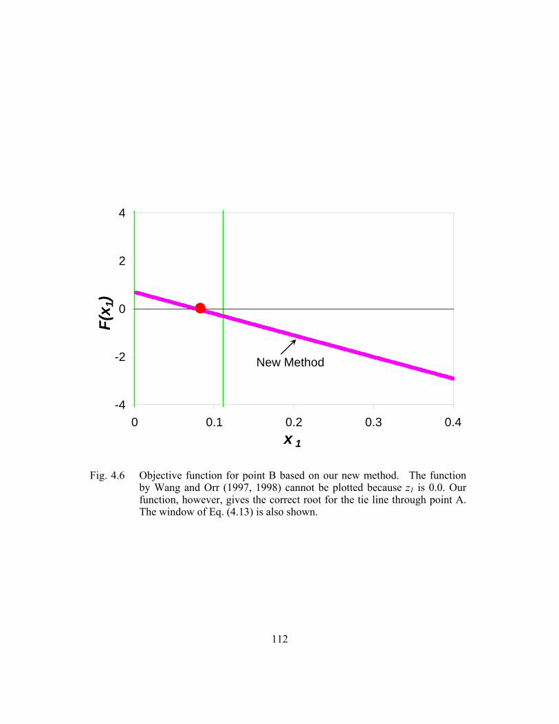
112
-4
-2
0
2
4
0 0.1 0.2 0.3 0.4x 1
F(x 1
)
New Method
Fig. 4.6 Objective function for point B based on our new method. The function by Wang and Orr (1997, 1998) cannot be plotted because z1 is 0.0. Our function, however, gives the correct root for the tie line through point A. The window of Eq. (4.13) is also shown.

113
-4
-2
0
2
4
-4 -2 0 2 4V
F(V)
Fig. 4.7 Rachford-Rice (1952) function for point C in Fig. (4.1). The root shown lies within the Whitson-Michelsen window (1989). The solution is greater than 1.0 because it is outside the two phase region where only vapor exists.

114
-4
-2
0
2
4
0 0.1 0.2 0.3 0.4x 1
F(x 1
)
New Method
Wang-Orr
Fig. 4.8 Objective functions for point C based on our new method and that given by Wang and Orr (1997, 1998). The correct root lies within the window given by Eq. (4.13).

115
-4
-2
0
2
4
-4 -2 0 2 4V
F(V)
Fig. 4.9 Rachford-Rice (1952) function for point D in Fig. (4.1). There is no root within the Whitson-Michelsen (1989) window. Outside the window, there is a root, but it is nonphysical, i.e. one equilibrium phase composition is negative.

116
-4
-2
0
2
4
0 0.1 0.2 0.3 0.4x 1
F(x 1
)
New Method
Wang-Orr
Fig. 4.10 Objective functions for point D based on our new method and that given by Wang and Orr (1997, 1998). The correct root lies just within the window given by Eq. (4.13), while only the trivial root exists for Wang and Orr (1997, 1998).

117
0.00 0.10 0.20 0.30 0.40 0.50 0.60 0.70 0.80 0.90 1.00
3
1
2
E
Fig. 4.11 Ternary phase behavior with K1 =1.0+2ε, K2 =1.0+ε, and K3 =1-ε and ε=10-9. The two phase region shown is very small and appears as a line in this diagram. The solid line is the tie-line extension through E.
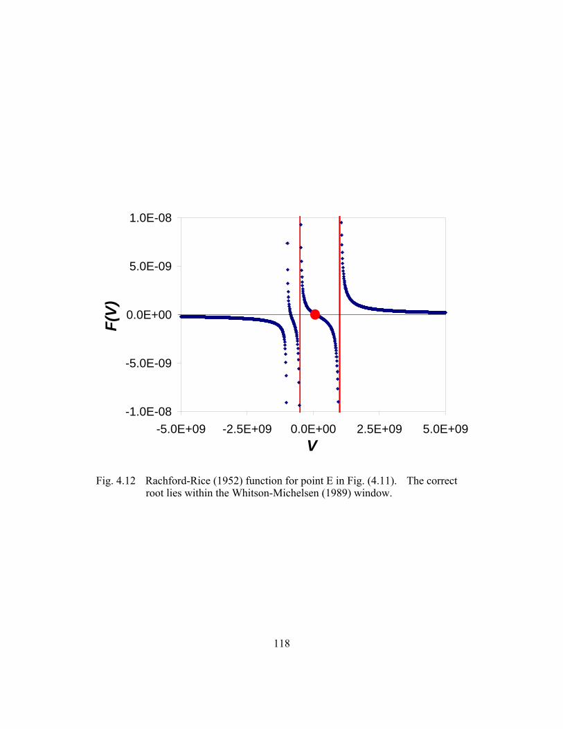
118
-1.0E-08
-5.0E-09
0.0E+00
5.0E-09
1.0E-08
-5.0E+09 -2.5E+09 0.0E+00 2.5E+09 5.0E+09V
F(V)
Fig. 4.12 Rachford-Rice (1952) function for point E in Fig. (4.11). The correct root lies within the Whitson-Michelsen (1989) window.

119
-2
-1
0
1
2
0 0.1 0.2 0.3 0.4x 1
F(x 1
)
-1.E-09
-5.E-10
0.E+00
5.E-10
1.E-09
New Method
Wang-Orr
Fig. 4.13 Objective functions for point E based on our new method and that given by Wang and Orr (1997, 1998). The correct root lies within the window given by Eq. (4.13). Wang and Orr’s method (1997, 1998) could mistakenly converge to the trivial root.

120
0.00 0.50 1.00C10
C1
C60.00 0.50 1.00C10
C1
C6
Fig. 4.14 Ternary diagram at 1015 psia and 440 oF for C1-C6-C10 system. Flash calculations with Peng-Robinson EOS (1977, 1978) converge to overall compositions within double precision values of the critical point (see triangular region).

121
0
2
4
6
8
10
0 5 10 15Number of Components
CPU
Tim
e (u
s)
Rachford-RiceLeibovici-NeoschilNew Method
Fig. 4.15 Comparison of the average CPU time for one flash calculation as a function of the number of components in the fluid. The new method is significantly faster than both Rachford-Rice (1952; Whitson and Michelsen, 1989) and Leibovici-Neoschil (1992).

122
0
2
4
6
8
10
0 5 10 15Number of Components
Num
ber o
f Ite
ratio
ns
Rachford-RiceLeibovici-NeoschilNew Method
Fig. 4.16 Comparison of the average number of iterations required for convergence for each method as a function of the number of components. Leibovici-Neoschil (1992) and the new method give about the same number of iterations.

123
0
0.5
1
1.5
2
0 5 10 15Number of Components
CPU
Tim
e pe
r Ite
ratio
n (u
s)
Rachford-RiceLeibovici-NeoschilNew Method
Fig. 4.17 Comparison of the average CPU time per iteration for each method as a function of the number of components. The new method is much faster than Leibovici-Neoschil (1992), but slower than Rachford-Rice (1952; Whitson and Michelsen, 1989).

124
-5.0E-05
-2.5E-05
0.0E+00
2.5E-05
5.0E-05
-2.E+05 -1.E+05 0.E+00 1.E+05 2.E+05
V
F(V)
Fig. 4.18 Rachford-Rice (1952) function for the K-values and overall composition given in Table (4.1). The function is highly nonlinear and the root lies just within the Whitson-Michelsen (1989) window (red vertical lines) near the pole.

125
-1
-0.5
0
0.5
1
0 0.1 0.2 0.3 0.4 0.5x 1
F(x 1
)
-1.E-04
-5.E-05
0.E+00
5.E-05
1.E-04
New M th d
Wang-Orr
Fig. 4.19 Objective functions for the fluid given by Table (4.1) based on our new method and that given by Wang and Orr (1997, 1998). The correct root lies just within the window given by Eq. (4.13). Wang and Orr’s method (1997, 1998), however, could converge to the trivial root.

126
-4
-2
0
2
4
0 0.25 0.5 0.75 1
V
F(V)
Fig.4.20 Rachford-Rice (1952) function for fluid given by Table (4.2). Convergence for V requires 18 iterations from an initial guess of 0.5. Convergence is difficult because the function is nonlinear and the root is near the right window limit.

127
-2
-1
0
1
2
2.E-03 4.E-03 6.E-03 8.E-03 1.E-02
x 1
F(x 1
)
Fig. 4.21 The objective function for the new method based on the fluid in Table (4.2). Convergence is achieved in 6 iterations even though the root is near a pole. The pole is just outside the window given by Eq. (4.13).

128
Chapter 5: Phase Behavior for Limited Compositional Simulators
Another approach to speed up compositional simulation is to implement non-
iterative flash calculations. Such an approach designed to be nearly as fast as black-oil
models while achieving improved accuracy in modeling miscible floods. As a result,
more grid blocks could be used than in standard compositional models at the expense of
modeling many components. This approach also has potential use in modeling chemical
floods.
In this chapter, a new phase behavior model for ternary systems is developed, and
then applied to several gas and surfactant flooding examples to illustrate its accuracy and
efficiency. Equation-of-state calculations are used only to generate the required
parameters for the limited compositional model. This approach is implemented in
UTCOMP and the results are compared to standard compositional simulation.
5.1 SIMPLIFIED PHASE BEHAVIOR MODEL
In this section, a simplified phase behavior model is presented using
transformation factors. First, we demonstrate the use of transformation factors for a
single composition. This transformation is then applied to tie lines in a ternary system,
such that all tie lines become parallel on ternary diagrams. Last, the non-iterative flash
calculation procedure is outlined using several simplified functions that describe the
proposed transformation factors.

129
5.1.1 Transforming a Composition
For a given composition zi in a ternary system, the following transformation using
a constant α can be made (Hand, 1930). First, we multiply iz by a constant factor,
which we name the transformation factor α . Thus,
1 1 2 2 3 3, , Z z Z z Z zα= = = .
We then normalize the resulting composition so that it sums to 1.0. That is, the
transformed composition *Z becomes:
( )
( )
( )
* 1 11
1 2 3 1
* 22
1
* 33
1
1 1
1 1
1 1
z zZz z z z
zZz
zZz
α αα α
α
α
= =+ + − +
=− +
=− +
. (5.1)
There is one-to-one correspondent between *Z and z for a given transformation
factor α . Thus, the inverse is unique and the corresponding actual compositions are
calculated from the transformed composition by:
( )( )( )
*1
1 *1
*2 2 1
*3 3 1
1
1 1
1 1
ZzZ
z Z z
z Z z
α α
α
α
=− −
= − +⎡ ⎤⎣ ⎦= − +⎡ ⎤⎣ ⎦
. (5.2)

130
The physical meaning of the transformation space is to stretch or shorten one of
the apex’s of the ternary diagram.
5.1.2 Transforming a Tie Line
The above transformation for an overall composition yields no simplification in
phase behavior. However, the same idea is applicable to a tie line. Given a tie line
with equilibrium compositions of ix and iy in a ternary system, the same
transformation factor is used for all the compositions along that tie line. The value of
the transformation factor is determined so that the tie line is parallel to one of the axis of
the ternary diagram, in this case the 1-3 axes. The objective of this transformation is to
simplify the phase behavior in such a way that flash calculations of the equilibrium
compositions would require no iteration. As shown before, the idea came from Hand
(1930), but he assumed that all tie lines were parallel in real compositional space so that
only one value of α is needed. In this research, however, the transformation factors
are dependent on compositions (each tie line has a different value of α ) so that real
phase behavior can be modeled.
One practical way to achieve non-iterative flash calculations is to make tie lines
parallel in transformed space by applying different transformation factor to each tie line.
For a ternary system, the transformed intermediate composition should be the same along
the same tie line, that is,
( ) ( )* * *2 22 2 2
1 11 1 1 1x yX Y Z
x yα α= = = =
− + − + . (5.3)
Thus, we can solve for α as:

131
( )2
2 1 1
11 KK K x
α −= +
− . (5.4)
The transformation factor is related to the tie-line slope through K-values and
binodal curves through 1x . The combination of a proper value for the transformation
factors and good models for the binodal curves in transformed space can yield
equilibrium compositions without iterations. This process is described in the following
section.
5.1.3 Flash Calculations Using Transformation Factors
In this section, the approach for non-iterative flash calculations is outlined. We
assume that the values of the transformation factors are evaluated so that all tie lines are
parallel to the 1-3 ternary base. For an arbitrary overall composition iz with a
transformation factor α , the intermediate composition in the transformed space can be
calculated using:
( )* * * 22 2 2
11 1zX Y Z
zα= = =
− + . (5.5)
To do flash calculations, the binodal curves in the transformed space are modeled using any arbitrary functions ( )* * *
1 1 2X X X= and ( )* * *1 1 2Y Y Y= . There is no restrictions
on the type of functions used, the functions could be a polynomial of any degree. Once
the functions are specified we can solve for *1X and *
1Y . From Eqs. (5.2), equilibrium
compositions can then be transformed back to the actual compositional space using:

132
( )( )
*1
1 *1
*2 1 2
3 1 2
1
1 1
1
XxX
x x X
x x x
α α
α
=− −
= − +⎡ ⎤⎣ ⎦= − −
(5.6)
and
( )( )
*1
1 *1
*2 1 2
3 1 2
1
1 1
1
YyY
y y Y
y y y
α α
α
=− −
= − +⎡ ⎤⎣ ⎦= − −
. (5.7)
The equilibrium compositions are exact if the transformation factors are
calculated accurately and the binodal curves are modeled exactly. In practice, the
binodal curves and the transformation factors are not modeled exactly, leading to a small
error in the calculated equilibrium compositions. Examining the definition of the
transformation factor in Eq. (5.3), we have:
( )( )
( )2 1* 2
21 11 1 1 1
x xxXx xα α
= =− + − +
(5.8)
which shows a relationship between α and *2X . In addition, the critical point in
transformed space is always at the maximum of the transformed intermediate
composition on the α vs. *2X plot. Experimental data or cubic EOS are first used to
calculate the transformation factor of a tie line using Eq. (5.4). The transformed
intermediate compositions are then calculated using Eq. (5.8). We describe that
relationship using simple functions as follows.

133
5.1.3.1 Linear Model for Transformation Factors
The simplest model that can be used to model the α and *2X relationship is the
linear model,
( )*2 1X A B α= + − , (5.9)
where A and B are determined by regression of the data to the linear function of Eq.
(5.9). From Eq. (5.5), where * *2 2X Z= , the following must be met:
( ) ( )2
1
11 1z A B
zα
α= + −
− + . (5.10)
Re-arrangement of Eq. (5.10) gives a quadratic function:
( ) ( )[ ] ( )21 1 21 1 0Bz Az B A zα α− + − + + − = , (5.11)
which yields the following two possible solutions:
( ) ( ) ( )21 1 1 2
1
41
2Az B Az B Bz A z
Bzα
− + ± + − −= + . (5.12)
There are two solutions of Eq. (5.12) either real or imaginary. Only the real
solutions are considered. As mentioned earlier, the critical point in transformed space is
always at the maximum of the transformed intermediate composition on the α vs. *2X
plot. Thus, the transformation factors must be within a pre-determined range from that
of the critical tie line to the base tie line (the tie line that lies on the 1-3 axis). The

134
transformation factor for the base tie line is determined in the limit as the base tie line is
approached. The transformation factor for the critical tie line can be evaluated when the
slopes of the binodal curves at the critical point are specified. The range in which the
correct solution of α must lie is temperature and pressure dependent. The calculated
real solutions for α using Eq. (5.12) are then compared with the pre-determined range.
There are several possibilities:
1. Only one real solution is within that range. The overall composition is
along a tie line or its extension. If this is the case, the equilibrium
compositions in the transformed space can be non-iteratively calculated
using the procedure outlined earlier;
2. Both real solutions are within that range. This case indicates that the
overall composition is on two tie lines, and thus in the single phase region.
This is because two tie lines cannot intersect in the two-phase region.
Both tie lines are found using the different α ’s;
3. None of the solutions are within the appropriate range, or there are no real
solutions to Eq. (5.11). This means that the overall composition is
beyond the critical point in the single-phase region and outside the region
of tie-line extensions.
5.1.3.2 Quadratic Model
Quadratic models can be used to improve the accuracy of the fit to the α and *2X relationship. That is:
( ) ( )2*2 1 1X A B Cα α= + − + − , (5.13)

135
where A, B and C are determined using the same procedure in Section (5.1.3.1). A
cubic equation results in terms of α :
( ) ( )( ) ( )( ) ( )3 21 1 1 21 1 1 0CZ C BZ B AZ A Zα α α− + + − + + − + − = . (5.14)
A cubic solver is needed for the solution of Eq. (5.14). There are three solutions
of α possible, and only real roots are considered. The approach to determine the
correct α used here is slightly different from that in Section (5.1.3.1). There are
several possibilities:
1. Only one real solution is within the range of maximum and minimum of
α . The overall composition is along a tie line or its extension. As a
result, the equilibrium compositions in the transformed space are non-
iteratively calculated using the procedure outlined earlier;
2. There are two or three real roots. This case indicates that the overall
composition is on the extensions of two tie lines, and thus in the single
phase region. This is because two tie lines cannot intersect in the two-
phase region. Both tie lines are found using the different α ’s;
3. None of the solutions are within the appropriate range. This means
that the overall composition is beyond the critical point in the single-
phase region and outside the region of tie-line extensions.
5.1.3.3 Reverse Cubic Function
A four-parameter function can also be used to model the *2X and α relationship
if more accuracy is desired:

136
( ) ( ) ( )2 3*
2 1/ 1 1 1X A B C Dα α α⎡ ⎤= + − + − + −⎣ ⎦ . (5.15)
Equation (5.15) results in the following cubic equation,
( ) ( ) ( )( ) ( )3 22 2 2 1 21 1 1 1 0DZ CZ BZ Z AZα α α− + − + − − + − = . (5.16)
A cubic solver is again required to determine the solution to Eq. (5.16). A
similar approach to determine the correct α is used here as in Section (5.1.3.2)
5.1.4 Reference Component in Transformation Method
In the above derivation, we apply transformation factors to the most volatile
component. However, we can also apply the same method using the least volatile
component. We assume that in both cases, the *2X and α relationship can be
accurately modeled. Even though the transformation factors for a particular tie line has
a different value using either the most or the least volatile components as reference, the
calculated equilibrium compositions are exactly the same regardless of the reference
component used.
5.1.5 Calculation Procedure
The calculation procedure using the transformation method is as the following:
1. Calculate equilibrium compositions using EOS or obtain from
experimental data. Calculate transformation factor using Eq.(5.4), and
the transformed intermediate composition by Eq. (5.3) for each tie line;

137
2. Regress transformation factors and transformed intermediate
compositions using one of the functions in Section (5.1.3) or some
other simple equations. Extrapolate the transformation factor at the
base tie-line and evaluate that at the critical tie-line;
3. Evaluate the coefficients of the equilibrium compositions for the
binodal curves in the transformed space as functions of pressure and
temperature if needed. Any accurate function is workable;
4. Solve the polynomial equations in step 2, and obtain the correct one
based on the analysis in Section (5.1.3) when multiple solutions exist;
5. Calculate the equilibrium compositions on the binodal curves in the
transformed space using the functions in step 3;
6. Translate the equilibrium compositions back into the conventional
space using Eqs.(5.6) and (5.7).
5.2 STABILITY ANALYSIS IN TRANSFORMATION MODEL
In EOS flash calculations, we use stability analysis to find whether a phase-split
calculation is needed or not. Stability analysis calculations are iterative as well. In this
new method, we do not need to perform a stability analysis by finding the stationary
points of the TPD function. We can determine whether the overall composition is stable
or not using the transformation method. The overall composition is in the two-phase
region, only when (1) one real solution for the transformation factor in that range; and (2)
the overall composition lies between the equilibrium compositions in transformed space.
In any other cases, the overall composition is stable and in the single-phase region.
Thus, the transformation method effectively eliminates the stability analysis calculations.

138
5.3 EXAMPLE FLASH CALCULATIONS
We illustrate the new method first for a ternary synthetic oil. A surfactant
flooding example is then presented using the transformation method. Phase behavior
calculations at different pressures are carried out. We also demonstrate the use of the
method when very little experimental data is available, i.e., only two tie lines are
available. The transformation method is also applied to a partial miscible case where
there is no critical point. The transformation method is last implemented in UTCOMP
to illustrate the accuracy and speed for a ternary case with varying pressures.
5.3.1 A C2-nC4-nC10 Ternary Synthetic Oil
Consider first a synthetic oil of C2-nC4-nC10 at 498.03 K and 6.125 MPa. Figure
(5.1) gives the ternary diagram using the Peng-Robinson EOS (1978) for this oil. Table
(5.1) lists the critical properties for the Peng-Robinson EOS (1978). All the BIPs are
zero. The tie lines and binodal curves are shown in Fig. (5.2) after the transformation
method is applied to the C2 component. The transformation causes all tie lines to be
parallel to the base tie line (where nC4 composition is zero) as shown in Fig. (5.2). The
critical point occurs at the maximum value of nC4 in the transformed space. The *2X
and α relationship is illustrated in Fig. (5.3), and then regressed using a quadratic
function. Table (5.2) compares some calculated equilibrium compositions by Peng-
Robinson EOS (1978) with those by the new transformation method. For a given
overall composition, the *2X value as a function of the transformation factor is shown in
Fig. (5.4) where the solid line is from the fitted quadratic curve and the dash line uses Eq.
(5.2). The transformation factor at that overall composition can thus be calculated by
finding the root when we equate both functions. Figure (5.5) shows that the equilibrium
compositions by the new method are very accurate. The maximum relative error in

139
calculated equilibrium compositions of this simple method compared to Peng-Robinson
EOS (1978) is less than 4%, with an average error less than 0.5%.
The transformation method could also be expressed based on the nC10 component.
The transformed binodal curves are shown in Fig. (5.6), and the *2X and α relationship
in Fig. (5.7). The flash calculations are still reasonably accurate as is shown in Fig.
(5.8). The average relative error of the transformation method is less than 1% with the
maximum less than 5%. The accuracy is increased slightly when C2 is used because in
this example the dew point curve is less accurately modeled than the bubble point curve
in the transformed space.
The new method is remarkably faster than conventional flash calculations with
three components. The equilibrium calculation for one overall composition requires
approximately 50 micro-second in the conventional EOS method, but less that 0.5 micro-
second in the transformation method. This is approximately 100 times improvement in
speed using the new method. Although not shown here, it is likely that the speedup will
increase significantly if more components were modeled. Also, because no iterations
are used in the transformation method, convergence is always achieved in flash
calculations. For the cases studied, the speed and robustness is substantially enhanced
without significant sacrifice of accuracy.
5.3.2 Surfactant Flooding
This model can also be applied to surfactant flooding to replace the iterative
Hand’s model (1930). For example, at a particular salinity the equilibrium compositions
for the excess and microemulsion phases is shown in Fig. (5.9) The calculated α and
transformed compositions are given in Fig. (5.10). For this case, the *2X and α
relationship can be accurately expressed using a reverse quadratic function:

140
( ) ( )2* 1/ 0.0611 1 7.7161 1 32.511surfC α α⎡ ⎤= − + − −⎣ ⎦ . (5.17)
This problem can be accurately solved using the non-iterative method.
Compared with the original experimental data, this approach gives very accurate results
without iteration as is illustrated in Fig. (5.11).
We also compare our new transformation method to Hand’s plot. Hand’s plot
for this case is shown in Fig. (5.12). This figure clearly indicates that Hand’s
approximation (1930) is reasonable (this is not always the case). However, in Hand’s
model, the bubble-point curve and dew-point curve must lie on the same line while in this
example they fall on slightly different lines. Calculations using Hand’s method are
complex and take significant time, mainly due to required iterations. Figure (5.13)
compares the computation result for the phase compositions using Hand’s method (1930)
and that from the original experimental data. Comparison of Figs. (5.13) and (5.11)
shows that Hand’s method (1930) is less accurate than the transformation method. It is
also approximately 10 times slower than the proposed transformation method.
5.3.3 Phase Behavior at Multiple Pressures
In reservoir simulations, the reservoir pressure can vary spatially and with time.
Temperature is assumed constant. Thus the constants in the transformation method must
be pressure dependent to account for the change in phase behavior with pressures. In
this example, a ternary system composed of C1, nC4 and nC10 are examined at different
pressures. The binodal curves are shown in Fig. (5.14) at pressures of 2000, 2500, 3000,
3500 and 4000 psia. The temperature is constant at 150oF. The tie lines are not plotted

141
in this figure; however, they are used to calculate the corresponding transformation
factors.
At each pressure, the transformation is applied, and the required coefficients as
functions of pressure are calculated using regression. The transformation factors and the
intermediate composition are illustrated in Fig. (5.15). The figure clearly demonstrates
that the critical tie line always has the largest transformed intermediate composition.
The base tie line always has zero nC4 composition. In addition, the transformed nC4
composition at the critical tie line decreases as pressure increases. That satisfies the
same feature in the phase envelope curves in Fig. (5.14), where at the critical points the
intermediate composition decreases with an increasing pressure. All the coefficients are
regressed using the following quadratic equations for this ternary system at 150oF:
( ) ( )2*
4
5 2 2
5 2 2
5 2 2
1 1
-2.686 10 4.337 10 - 58.66-1.116 10 1.467 10 - 24.24-1.607 10 3.020 10 - 34.97
nC A B C
A P PB P PC P P
α α− −
− −
− −
= − + − +
= × + ×
= × + ×
= × + ×
. (5.18)
It is also important to locate the highest and lowest values of the transformation
factor to determine how many phases are present. The end points of the transformation
factors vary with pressure and have these forms (see Fig. (5.16)):
( )( )
8 2 4min
9 2 5max
1 -1.461 10 1.412 10 - 1.206
1 -2.422 10 1.181 10 - 0.8495
P P
P P
α
α
− −
− −
− = × + ×
− = × + × . (5.19)
All information needed to calculate the transformation factor and the transformed
intermediate composition is now known. In the next step, the binodal curves are

142
transformed to the new compositional space. The transformed bubble-point curve is
plotted in Fig. (5.17) ( *10nC as a function of *
4nC ), and dew-point curve in Fig. (5.18)
( *1C as a function of *
4nC ). One can interpolate the binodal curves accurately or use
any other appropriate functions to model them. In this example, a quadratic function is
used to model the binodal curves.
The calculated equilibrium compositions using the transformation procedure are
compared with the calculations using Peng-Robinson EOS (1977, 1978) at a pressure of
3000 psia. The only difference from the example of Section (5.2.1) is that all required
coefficients are now pressure-dependent functions instead of constant values. Figure
(5.19) shows that the transformation method accurately captures both the binodal curves
and the tie lines at this pressure. More important, the new method requires less than 0.5
micro-second in computational time, while the Peng-Robinson EOS (1977, 1978)
requires 150 times more time.
5.3.4 Flash Calculations with Limited Data
The transformation method can be applied reasonably well as long as at least two
tie lines are available. In this research, we use the method when only the base and
critical tie lines are available. Linear interpolation of α is then used since there is no
information on tie lines in between.
In this example, we use the same ternary system as in Fig. (5.14) with this
simplification. The transformation factor relationship is re-plotted to show their linear
dependence in the transformation space in Fig. (5.20). The dependence of the
coefficients on the pressure is still non-linear and can be interpolated accurately using the
following quadratic equations:

143
( )*4
7 2 4
7 2 4
1
-7.207 10 7.493 10 - 3.420-5.806 10 8.484 10 - 2.703
nC A B
A P PB P P
α− −
− −
= − +
= × − ×
= × − ×
. (5.20)
The minimum and maximum of the transformation factors are unchanged as in
Eqs. (5.20). In addition, the binodal curves are straight lines in the transformed space
rather in the actual compositional space. Figure (5.21) shows for the bubble point curve
and Fig. (5.22) for the dew point curve from the base tie line to the critical tie line. The
simplified transformation method is then implemented to calculate the equilibrium
compositions at 3000 psia. The result is compared with the original equilibrium
compositions by Peng-Robinson (1977, 1978) EOS in Fig. (5.23). Figure (5.23)
demonstrates the accuracy of this simplified model that is based on only these two tie
lines. Although speedup is slightly greater using this approach, the benefit is minimal.
5.3.5 Implementation with Real Fluid Experimental Data
This section compares the results of the transformation method to experimental
results. Table (5.4) shows an experimental data of equilibrium compositions of nC4-
CO2-nC10 system (Metcalfe and Yarborough, 1978). In this example, we use the method
in Section (5.3.4) that only two tie lines are used at each pressure of 1000 and 1400 psia.
The four tie lines used to initialize the calculation is highlighted in grey in Table (5.4).
In addition, we assume that the simplified linear correlation exists for *2X and α
relationship for the four tie lines. The values of transformation factor and intermediate
composition are shown in Fig. (5.24). The maximum and minimum of the

144
transformation factors are assumed linearly dependent on reservoir pressure. The
binodal curves (Fig. (5.25)) are straight lines in transformed space.
Figure (5.26) compares the equilibrium compositions by the transformed method
with the experimental data at pressures of 1000 and 1400 psia. In Fig. (5.27), the
equilibrium compositions at 1500 psia are calculated and compared with the experimental
data. The compositions calculated are less accurate than that in Fig. (5.26), but can be
improved by using a non-linear equation to estimate the maximum and minimum of α ,
given that more experimental data are used. Errors also result because the experimental
data often have noise compared with EOS calculations. However, it is still reasonably
accurate considering that only four tie lines in total are used (two tie lines each at the
pressures of 1000 and 1400 psia).
5.3.6 Flash Calculations with Constant K-values
The new method can also be implemented to calculate the equilibrium
compositions when K-values are constant. Compared with constant K-value flash
calculations in Chapter 4 which are iterative, the new method is non-iterative. Because
K-values are constant, only two tie lines are required to exactly model this example.
In this example, the following K-values are used: 1 5.0K = , 1 2.0K = and
3 0.5K = . The phase behavior is illustrated in Fig. (4.1). The *2X and α relationship
is plotted in Fig. (5.29), and can be exactly expressed as:
( )*2 0.75 / 1 0.25C α= − − + . (5.21)
The binodal curves are also exactly described using the following linear functions:

145
( )( )
* *1 2
* *1 2
1 / 3
5 16
x C
y C
= −
= − . (5.22)
The binodal curves are straight lines in compositional space when the K-values
are constant. This is also true in transformed space. The determined binodal curves
from the simplified transformation method, compared with that from constant K-value
flash calculations is illustrated in Fig. (5.29), which shows an exact match. The new
method, however, is approximately 10 times faster than the constant K-value flash
calculations and is robust because no iterations are required.
5.3.7 Simulation Comparison
We also implemented the new transformation method into UTCOMP, an IMPEC
reservoir simulator using the same ternary system as in Section (5.3.3). The reservoir is
100 ft by 25 ft by 25 ft, with constant porosity of 16% and homogeneous permeability of
25 mD. The injection and initial fluid compositions are listed in Table (5.5). The
reservoir temperature is constant at 150oF and the initial reservoir pressure is 3000 psia.
The injection well BHP is fixed at 4000 pisa and the production well pressure at 2000
psia. The 1-D simulations used a constant time step of 0.005 days. Phase densities are
still calculated using the EOS while phase viscosities are calculated using the Lohrenz-
Bray-Clark correlation (1964). The phase densities and viscosities, however, could be
regressed in transformation space.
Figures (5.30) – (5.32) show the nC10 component recovery, average reservoir
pressure and compositions at the production well as a function of simulation time using

146
standard flash calculations and the transformation method. The new method is nearly
identical to standard compositional simulations.
The pressure profiles at 20 and 40 days (corresponding to approximately 0.15 and
0.33 pore volume injected) are shown in Figs. (5.33) and (5.34). The overall
composition profiles at these time steps are also plotted in Figs. (5.35) and (5.36). All
figures showed that the new transformation method has similar accuracy as using
standard UTCOMP simulations.
We also tested the speed for a varying number of grid blocks using a 1.3 GHz
CPU with 1.5G RAM. The CPU time used for flash calculations alone (including
stability analysis) is shown in Fig. (5.39) for 10, 20 and 40 grid blocks in the x-direction.
The CPU time required for the entire simulation, flash calculations and density
calculations is given in Table (5.6). The total CPU time for the simulation using the new
transformation method is approximately twice faster than the standard method, mainly
because the flash calculation in this example is about 50% of total simulation time. The
new transformation method is approximately 10 to 11 times faster than standard
UTCOMP in the flash calculations (including stability analysis and density calculation).
This is much less than the speedup in the batch calculations, mainly because: (1) densities
are calculated from Z-factors using EOS; and (2) standard flash calculations in the
simulation uses the values from the previous time step. The computation time for the
equilibrium compositions using the transformation method is approximately 50 times
faster than EOS flash calculations. If phase densities and viscosities are regressed in the
transformed space, the simulation time using the transformation method would be less.

147
5.4 CONCLUSIONS
In this chapter, a new non-iterative transformation method is developed to
calculate the equilibrium compositions for ternary systems. The new method is much
faster than EOS flash calculations because the transformation method is non-iterative.
The new method is robust since there is no iteration and will always converge. This
method is also very accurate when compared to an EOS model. Moreover, stability
analysis calculations are eliminated because the direct solution determines whether one or
two phases are present.
Simulation results confirm the speed and accuracy of this new model. The flash
calculation is approximately six to ten times faster than the conventional method. The
accuracy of the simulation is nearly perfect and is more realistic than if a black-oil model
had been used. This method may be useful for large-scale, fine-grid miscible flooding
simulations.

148
TC (oF) PC (psia) ω
C2 90.05 708.35 0.098 nC4 305.69 551.10 0.193 nC10 652.01 305.68 0.490
Table 5.1 Input EOS critical properties for the ternary system in Fig. (5.1).

149
Bubble Point Curve Dew Point Curve
C2 nC4 nC10 C2 nC4 nC10 EOS 38.59 4.84 56.57 80.53 5.58 13.90 TM 38.57 4.84 56.58 80.51 5.58 13.92 EOS 36.78 9.69 53.54 74.86 11.14 13.99 TM 36.74 9.68 35.70 74.92 11.15 13.93 EOS 34.96 14.52 50.51 69.22 16.68 14.10 TM 34.96 14.52 50.52 69.33 16.69 13.98 EOS 33.14 19.37 47.50 63.60 22.18 14.22 TM 33.16 19.37 47.48 63.73 22.19 14.08 EOS 31.30 24.21 44.49 58.03 27.61 14.36 TM 31.33 24.21 44.46 58.14 27.63 14.23 EOS 29.46 29.07 41.47 52.52 32.96 14.53 TM 29.47 29.06 41.47 52.59 32.97 14.44 EOS 27.62 33.93 38.45 47.08 38.19 14.73 TM 27.59 33.93 38.48 47.07 38.19 14.73 EOS 25.79 38.82 35.39 41.72 43.28 15.00 TM 25.73 38.81 35.46 41.63 43.24 15.12 EOS 23.98 43.75 32.28 36.46 48.17 15.34 TM 23.93 43.75 32.32 36.27 48.10 15.63 EOS 22.20 48.80 29.00 31.30 52.80 15.90 TM 22.26 48.79 28.95 31.02 52.68 16.31 EOS 20.63 53.94 25.43 26.10 57.00 16.80 TM 20.79 54.04 25.17 25.88 56.90 17.21 EOS 20.03 58.68 21.29 21.50 59.60 18.90 TM 19.83 58.54 21.63 21.87 59.94 18.20
Table 5.2 Comparison of the phase envelope in Fig. (5.1) by Peng-Robinson EOS (1977, 1978) with the new method. With the transformation method, the relatively difference is usually less than 1% of the EOS equilibrium compositions, with the maximum less than 4%. TM indicates “Transformation Method”.

150
TC (oF) PC (psia) ω
C1 -116.59 667.20 0.008 nC4 305.69 551.10 0.193 nC10 652.01 305.68 0.490
Table 5.3 Input EOS critical properties for the ternary system in Fig. (5.8).

151
Bubble Point Curve Dew Point Curve
CO2 nC4 nC10 C2 nC4 nC10 47.87 18.41 33.73 94.54 5.23 0.23 48.37 10.46 41.17 97.06 2.77 0.17 47.94 26.44 25.62 91.97 7.58 0.18
1000 psia
49.21 37.24 13.56 87.23 12.60 0.94 68.02 8.29 23.69 96.75 2.89 0.37 68.52 12.80 18.68 94.87 4.39 0.75 67.87 13.97 18.16 94.14 5.30 0.57 70.96 17.90 11.14 90.61 8.71 0.68
1400 psia
76.28 20.30 3.42 86.06 12.97 0.97 60.90 9.27 29.83 96.91 2.80 0.29 60.23 15.93 23.84 94.34 5.28 0.38 62.31 21.91 15.78 91.58 8.06 0.37 65.20 27.45 7.35 87.47 12.08 0.45
1250 psia
67.27 29.43 3.30 84.69 14.97 0.34 71.41 7.22 21.37 96.18 3.13 0.69 73.16 10.57 16.28 94.78 4.45 0.78 73.25 12.42 14.33 93.06 6.00 0.95 76.30 13.94 9.76 91.73 7.29 0.99
1500 psia
79.92 15.10 4.98 89.04 9.94 1.02
Table 5.4 Experimental data used in the transformation method in section (5.3.5). Four tie lines (in grey) are used to initialize the calculation. All other data are used to illustrate the accuracy of the non-iterative transformation method.

152
Injection Gas Composition Initial Oil Composition C1 nC4 nC10 C1 nC4 nC10
0.95 0.05 0.0 0.0 0.6 0.4
Table 5.5 Initial oil composition and injection gas composition in the UTCOMP simulation for a ternary system.

153
CPU Time in second by UTCOMP
CPU Time in second Using TM
Speedup # of Grid
Blocks
Total Flash Total Flash Comp. Total Flash Comp.
10 21.69 9.22 12.31 0.93 0.23 1.76 9.9 40.1
20 33.08 17.02 16.78 1.51 0.38 1.97 11.3 44.8
40 57.20 31.58 28.12 2.85 0.62 2.03 11.1 50.9
Table 5.6 Comparison of CPU time using standard UTCOMP with the transformation method. The simulation using the transformation method is much faster. TM means “Transformation Method.”

154
nC10
C2
nC4
Fig. 5.1 Ternary diagram for C2-nC4-nC10 system at 498.03 K and 6.125 MPa. The equilibrium compositions are calculated using the Peng-Robinson EOS (1977, 1978).

155
nC10
C2
nC4
Fig. 5.2 Ternary diagram for C2-nC4-nC10 system in the transformed space at 498.03 K and 6.125 MPa. The transformation factor is applied to the C2 component. In the transformed space, all tie lines are parallel, and the critical point occurs when *
4nC is a maximum.

156
y = -2.593x2 - 4.322x - 0.991R2 = 1
0
0.2
0.4
0.6
0.8
1
-1 -0.8 -0.6 -0.4 -0.2 0
α-1
nC4*
Fig. 5.3 Transformation factors for C2-nC4-nC10 ternary system in Fig. (5.1). A quadratic function is very accurate to describe the curve.

157
y = -2.593x2 - 4.322x - 0.991R2 = 1
0
0.2
0.4
0.6
0.8
1
-1 -0.8 -0.6 -0.4 -0.2 0
α-1
nC4*
Fig. 5.4 Transformation factors for C2-nC4-nC10 ternary system in Fig. (5.1). The solid line uses the quadratic function, the dash line is that from Eq. (5.2) for an overall composition. The triangle is the correct transformation factor for the tie line passing through the overall composition.

158
nC10
C2
nC4
Fig. 5.5 Comparison of the equilibrium compositions for C2-nC4-nC10 system at 498.03 K and 6.125 MPa. The calculated values are in black, and the original data are in grey. The new non-iterative method yields almost identical results.
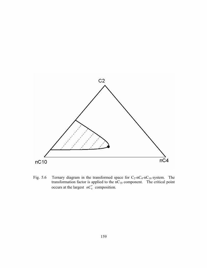
159
Fig. 5.6 Ternary diagram in the transformed space for C2-nC4-nC10 system. The transformation factor is applied to the nC10 component. The critical point occurs at the largest *
4nC composition.
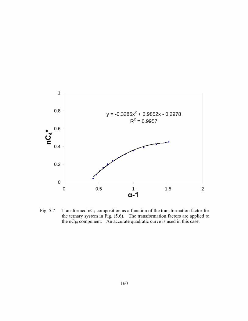
160
y = -0.3285x2 + 0.9852x - 0.2978R2 = 0.9957
0
0.2
0.4
0.6
0.8
1
0 0.5 1 1.5 2α-1
nC4*
Fig. 5.7 Transformed nC4 composition as a function of the transformation factor for the ternary system in Fig. (5.6). The transformation factors are applied to the nC10 component. An accurate quadratic curve is used in this case.

161
nC10
C2
nC4
Fig. 5.8 Equilibrium compositions computed by the transformation method when the transformation factors are applied to nC10 component. The original data (gray) are from the Peng-Robinson EOS (1977, 1978). The non-iterative transformation method yields accurate phase behavior (black).

162
Oil
Surfactant
Brine
Fig. 5.9 Ternary diagram for a brine-oil-surfactant ternary system with co-surfactant injected (Pope, et al. 1982). The tie lines are in dash lines and the original data are in triangles.

163
0.00
0.01
0.02
0.03
0.04
0.05
0 25 50 75 100
α-1
Csu
rf*
Fig. 5.10 Transformation factors for a surfactant system (see Fig. (5.9)). The transformation is applied to the oil component.

164
Fig. 5.11 Comparison of the non-iterative transformation method (diamonds with tie lines) with the experimental data (triangles).

165
1.E-02
1.E+00
1.E+02
1.E+04
1.E+06
1.E+08
1.E-02 1.E+00 1.E+02 1.E+04
Composition Ratio
Com
posi
tion
Rat
io
32 32
12 22
log vs logC CC C⎛ ⎞ ⎛ ⎞⎜ ⎟ ⎜ ⎟⎝ ⎠ ⎝ ⎠
32 31
22 11
log vs logC CC C⎛ ⎞ ⎛ ⎞⎜ ⎟ ⎜ ⎟⎝ ⎠ ⎝ ⎠
Fig. 5.12 Hand’s plot (1930) for the ternary diagram of chemical flood in Fig. (5.9).

166
Fig. 5.13 Comparison of Hand’s method (diamonds with tie lines) and the experimental data (triangles). Hand’s method is less accurate than the transformation method in Fig. (5.11).

167
nC10
C1
nC4
2000 psia
2500 psia3000 psia
3500 psia4000 psia
Fig. 5.14 Ternary diagram for C1- nC4 - nC10 system at different pressures from 2000 psia to 4000 psia at 150oF. The critical points at each pressure are shown by solid circles.

168
0
0.1
0.2
0.3
0.4
0.5
0.6
0.7
0.8
0.9
1
-1 -0.95 -0.9 -0.85 -0.8
α - 1
nC4*
2000 psia
2500 psia
3000 psia
3500 psia
4000 psia
Fig. 5.15 Transformed nC4 composition as a function of transformation factor for the ternary diagram in Fig. (5.14) at different pressures. The critical point is always at the maximum value for *
4nC .

169
-1
-0.95
-0.9
-0.85
-0.8
1000 2000 3000 4000 5000
Pressure (psia)
α-1
base tie-line
critical tie-line
Fig. 5.16 The minimum transformation factor (the critical tie line) and the maximum (the base tie line) as a function of pressure. The calculated transformation factors must lie within this range.

170
Fig. 5.17 Bubble-point curves in the transformed space at different pressures for the phase behavior in Fig. (5.14). All curves are accurately fitted using quadratic functions.

171
Fig. 5.18 Dew-point curves in the transformed space at different pressures for the phase behavior in Fig. (5.14). All curves are accurately fitted using quadratic functions.

172
Fig. 5.19 Equilibrium compositions calculated using the transformation method at pressure of 3000 psia and 150oF. The transformation method is accurate. The original data from the PR EOS (1977, 1978) is shown in grey and the calculated data using the transformed method is in black.

173
0
0.1
0.2
0.3
0.4
0.5
0.6
0.7
0.8
0.9
1
-1 -0.95 -0.9 -0.85 -0.8
α - 1
nC4*
2000 psia
2500 psia
3000 psia
3500 psia
4000 psia
Fig. 5.20 Transformed nC4 composition as a function of the transformation factor for the ternary system in Fig. (5.14) at different pressures. We linearly interpolate the relationship at each pressure from the base tie line to the critical tie line in this example.
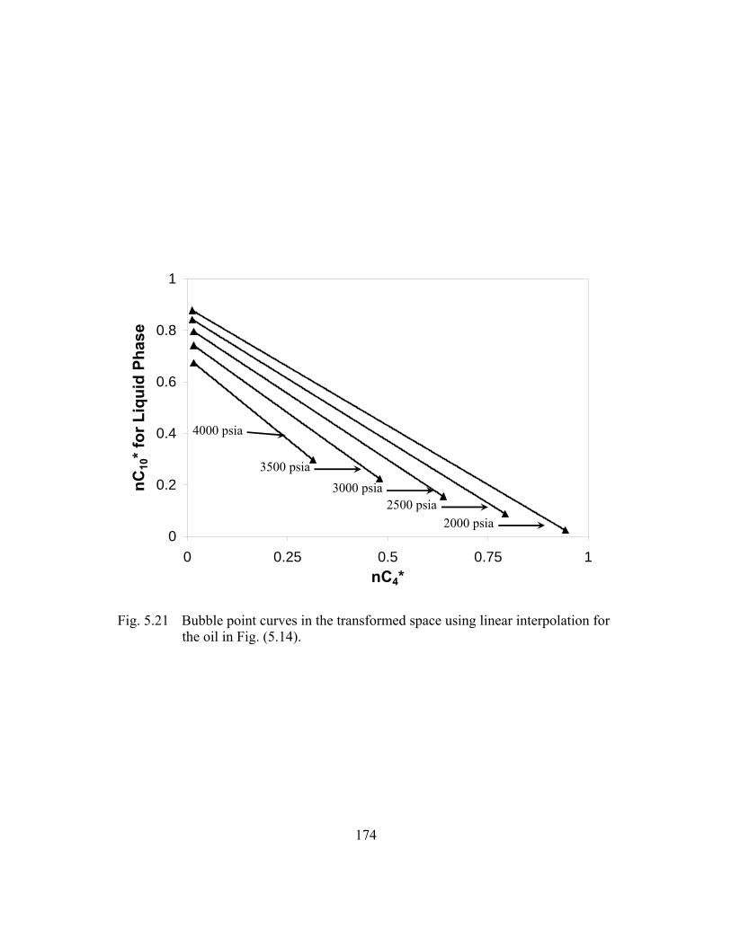
174
0
0.2
0.4
0.6
0.8
1
0 0.25 0.5 0.75 1nC4*
nC10
* for
Liq
uid
Phas
e
4000 psia
3500 psia3000 psia
2500 psia2000 psia
Fig. 5.21 Bubble point curves in the transformed space using linear interpolation for the oil in Fig. (5.14).

175
0
0.2
0.4
0.6
0.8
1
1.2
0 0.25 0.5 0.75 1
nC4*
C1*
for V
apor
Pha
se
4000 psia
3500 psia3000 psia
2500 psia2000 psia
Fig. 5.22 Dew point curves using linear interpolation in the transformed space for the oil in Fig. (5.14).

176
Fig. 5.23 Equilibrium compositions calculated using the transformation method at 3000 psia and 150oF. We linearly interpolate the phase behavior from the limiting tie line to the base tie line on the 1-3 axis. The transformation method using linear interpolation yields accurate results.

177
0
0.25
0.5
0.75
1
-1 -0.95 -0.9 -0.85 -0.8α -1
nC4*
Fig. 5.24 Transformed nC4 composition as a function of transformation factor for the CO2-nC4-C10 ternary system (Metcalfe and Yarborough, 1979) at 1000 psia (diamonds) and 1400 psia (triangles).

178
0
0.25
0.5
0.75
1
0 0.25 0.5 0.75 1nC4*
CO
2*
Fig. 5.25 Binodal curves in the transformed space at pressures of 1000 psia (diamonds) and 1400 psia (triangles). Linear interpolation is used for the binodal curves between two tie lines at each pressure.
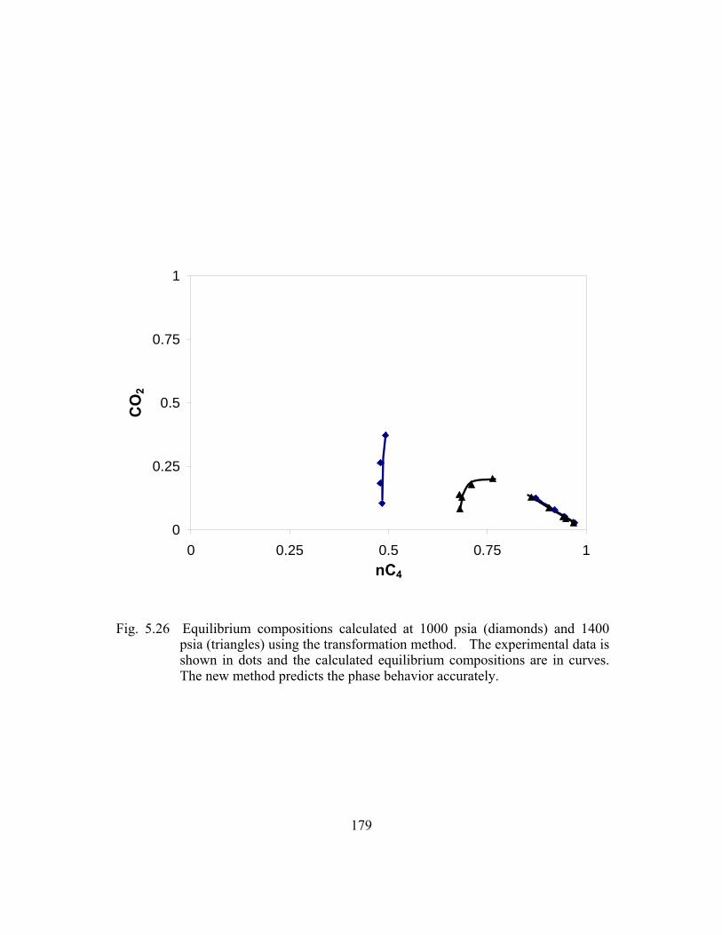
179
0
0.25
0.5
0.75
1
0 0.25 0.5 0.75 1nC4
CO
2
Fig. 5.26 Equilibrium compositions calculated at 1000 psia (diamonds) and 1400 psia (triangles) using the transformation method. The experimental data is shown in dots and the calculated equilibrium compositions are in curves. The new method predicts the phase behavior accurately.

180
0
0.25
0.5
0.75
1
0 0.25 0.5 0.75 1nC4
CO
2
Fig. 5.27 Equilibrium compositions calculated at 1250 psia (diamonds) and 1500 psia (triangles) using the transformation method. The experimental data is shown in dots and the calculated equilibrium compositions are in curves. The new method is accurate.

181
0
0.1
0.2
0.3
0.4
0.5
0 10 20 30 40 50α-1
C2*
Fig. 5.28 Transformed intermediate composition as function of the transformation factor for a ternary system with constant K-values of 1 5.0K = , 1 2.0K = and 3 0.5K = .

182
3
1
2
Fig. 5.29 Calculated equilibrium compositions using the transformed method for the ternary system with constant K-value in Fig. (4.1). Triangles are from the Rachford-Rice method (1952), and the lines are from the transformation method. The transformation method is very accurate.

183
0
0.25
0.5
0 10 20 30 40 50Time (days)
Rec
over
y
0
0.25
0.5
0 10 20 30 40 50Time (days)
Rec
over
y
0
0.25
0.5
0 10 20 30 40 50Time (days)
Rec
over
y
Fig. 5.30 Comparison of the C10 recovery using the standard EOS model (triangles) and the transformation method (lines) at different numbers of grid blocks. The numbers of grid blocks are 10, 20 and 40, respectively, from the top. The transformation method agrees well with the conventional method.
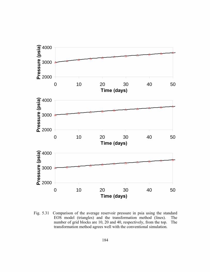
184
2000
3000
4000
0 10 20 30 40 50Time (days)
Pres
sure
(psi
a)
2000
3000
4000
0 10 20 30 40 50Time (days)
Pres
sure
(psi
a)
2000
3000
4000
0 10 20 30 40 50Time (days)
Pres
sure
(psi
a)
Fig. 5.31 Comparison of the average reservoir pressure in psia using the standard EOS model (triangles) and the transformation method (lines). The number of grid blocks are 10, 20 and 40, respectively, from the top. The transformation method agrees well with the conventional simulation.

185
0
0.5
1
0 10 20 30 40 50Time (days)
Com
posi
tion
0
0.5
1
0 10 20 30 40 50Time (days)
Com
post
ion
0
0.5
1
0 10 20 30 40 50Time (days)
Com
posi
tion
Fig. 5.32 Comparison of the compositions measured at the production well using the standard EOS model (triangles) and the transformation method (curves). The nC4 compositions are the solid lines, nC10 are the dash lines and C1 are the double dash lines.

186
2000
3000
4000
0 0.2 0.4 0.6 0.8 1XD
Pres
sure
(psi
a)
2000
3000
4000
0 0.2 0.4 0.6 0.8 1XD
Pres
sure
(psi
a)
2000
3000
4000
0 0.2 0.4 0.6 0.8 1XD
Pres
sure
(psi
a)
Fig. 5.33 Comparison of pressure profile at 20 days using 10 (top), 20 (middle) and 40 (bottom) grid blocks. The standard UTCOMP results are in triangles and the transformation method results are in curves. The non-iterative transformation method is almost identical as the conventional method.

187
2000
3000
4000
0 0.2 0.4 0.6 0.8 1XD
Pres
sure
(psi
a)
2000
3000
4000
0 0.2 0.4 0.6 0.8 1XD
Pres
sure
(psi
a)
2000
3000
4000
0 0.2 0.4 0.6 0.8 1XD
Pres
sure
(psi
a)
Fig. 5.34 Comparison of the pressure profile at 40 days using 10 (top), 20 (middle) and 40 (bottom) grid blocks. The standard UTCOMP results are in triangles and the transformation method results are in curves. The non-iterative transformation method is very accurate.

188
0
0.5
1
0 0.2 0.4 0.6 0.8 1XD
Com
posi
tion
0
0.5
1
0 0.2 0.4 0.6 0.8 1XD
Com
posi
tion
0
0.5
1
0 0.2 0.4 0.6 0.8 1XD
Com
posi
tion
Fig. 5.35 Comparison of the overall composition profile at 20 days using 10 (top), 20 (middle) and 40 (bottom) grid blocks. The standard UTCOMP results are in triangles. The results using the transformation methods are: nC4 in solid curves, nC10 in dash curves and C1 in double dash curves.

189
0
0.5
1
0 0.2 0.4 0.6 0.8 1XD
Com
posi
tion
0
0.5
1
0 0.2 0.4 0.6 0.8 1XD
Com
posi
tion
0
0.5
1
0 0.2 0.4 0.6 0.8 1XD
Com
posi
tion
Fig. 5.36 Comparison of the overall composition profile at 40 days using 10 (top), 20 (middle) and 40 (bottom) grid blocks. The standard UTCOMP results are in triangles. The results using the transformation methods are: nC4 in solid curves, nC10 in dash curves and C1 in double dash curves.

190
0
10
20
30
40
0 10 20 30 40 50Number of Grid Blocks
Flas
h C
alcu
latio
n Ti
me
(s)
Standard UTCOMP Model
Trasformation Model
Fig. 5.37 CPU time used for the flash calculations in simulation using the standard UTCOMP method and the transformation method. The new method is approximately 10 times faster than the conventional flash calculation.

191
Chapter 6: Conclusions and Future Work
In this work, several practical phase behavior models have been developed for
flash calculations using EOS, constant K-values, and non-iterative transformation factors.
The implementation of these different models and their impacts on speed, accuracy and
robustness were examined. Compared with conventional models, all these new
approaches show significantly improved speed and robustness.
6.1 KEY CONCLUSIONS
6.1.1 EOS-Based Reduced Method
1 A new, rapid, accurate, simple and robust model is developed to perform
flash calculations with arbitrary non-zero binary interaction parameters
(BIPs). The new model requires a maximum of six reduced variables in
phase-split calculations, and five in stability analysis calculations
regardless of the number of components;
2 In flash calculations, the new method significantly improves the speed by
a factor of 1.3 for seven-component systems, and approximately 14 for
thirty-five component systems compared with the conventional method.
In stability analysis calculations, the new method also improves the speed
by a factor of 1.9 for seven-component systems and 24 for thirty-five
component systems;
3 In flash calculations, the new method has improved robustness close to the
critical point;

192
4 In flash calculations, the reduced method will yield the exact solution
compared with conventional method when the same BIPs are used.
Significant improvement in speed and robustness without sacrificing
accuracy are the major advantages of this new method;
5 The new method is also shown to be easily applied to three-phase flash
calculations.
6.1.2 Constant K-value Flash Calculations
1 A simple, fast and accurate objective function is developed to replace
Rachford-Rice and similar approaches.
2 The correct solution lies within a predetermined window, the range of
which is derived in this dissertation;
3 The new objective function is continuous and almost linear in the solution
window. Because of improved linearity, the new method is significantly
faster than Rachford-Rice, and often requires less iterations. Based on
batch calculations, the research shows that the new method needs
approximately 25% less time for three-component fluids, and 40% less for
fifteen-component fluids;
4 The new objective function is scaled near the critical point so that neither
the objective function nor its derivative change significantly when K-
values approach 1.0;
5 Simulations in GPAS show that this new objective function requires
approximately 5% fewer iterations than the Rachford-Rice procedure;
6 The robustness is also improved that the new objective function can
always converge to a correct tie line regardless the overall composition.
193
6.1.3 Transformation Method for Limited Compositional Simulators
1 A simple, accurate, non-iterative, rapid and robust transformation method
is developed for ternary systems for limited compositional simulators;
2 The new method is over 100 times faster than conventional EOS flash
calculations, and approximately 10 times faster than flash calculations
with constant K-values. No iterations are used in calculating equilibrium
compositions. As a result this method is very fast and robust even at the
critical point.
3 An investigation window is proposed to guarantee the uniqueness of the
solution. This window is also used in phase stability test;
4 The new method can model both partial miscible and full miscible
flooding processes using pressure- and temperature-dependent
transformation factors and binodal curve functions. The new model is
much more accurate compared with Hand’s model, and almost exact as
EOS flash calculations;
5 Because the method is direct, the new method always gives an accurate
solution when the overall composition is on a tie line or tie-line extension;
6 Even with simplified transformation model by linear interpolation between
base tie line and critical tie line, the new method is practically accurate;
7 Reservoir simulations confirm that this model is much faster than
conventional EOS models without sacrificing accuracy. For example,
simulation shows that the new method is approximately 10 times faster
than the conventional flash calculations in UTCOMP for a ternary system;

194
8 The new method could be used to simulate miscible gas injection that
requires complicated phase behavior with a few pseudocomponents and
requires a large number of grid blocks. Some accuracy will be lost,
however, by using only three pseudocomponents.
6.2 FUTURE RESEARCH
Additional research that could be addressed are:
1 Implementation of the new reduced method into an IMPEC and fully
implicit reservoir simulator is of practical interest to illustrate the
efficiency and accuracy of this new model;
2 Implementation of the new reduced method for three or more phases is of
growing importance;
3 Optimization of the iterative techniques in reduced method is also
important, so that the number of iterations could further be reduced;
4 Expansion of the non-iterative transformation method to at least four
pseudocomponents would greatly improve its accuracy in compositional
reservoir simulations.

195
Appendix: Flash Calculations with Negative Compositions
When we calculate MMP or MME, it may require flash calculations with constant
K-values where at least one component has a negative overall composition. In this case,
there may be multiple tie lines passing through that overall composition and in
MMP/MME calculations it is important to locate all of them. The conventional method
using Rachford-Rice (1952) has convergence problems for these cases because the
correct solutions are not within the Whitson-Michelsen window (1989).
We can extend the new objective function in Chapter 4 to this case to guarantee
convergence. A similar investigation window can also be derived within which all
correct solutions must lie. Let us assume that the K-values of the overall composition
are sorted from the lightest component (with the largest K-value) to the heaviest component (with the smallest K-value), that is 1 1... 1 ...
Cj j NK K K K+> > > > > > .
The same objective function as Eq. (4.12) applies in this case. However, the
investigation window of Eq. (4.13) is different. From Eq. (4.7), we have for each
component in the equilibrium liquid phase
( )
( ) ( )1 1
1 1 1
1 2,..., 1
1i
i Ci i
K z xx i N
K z K K x−
= = −− + −
(A.1)
Further, we want 0 1ix≤ ≤ for each equilibrium composition. As a result,
( )
( ) ( )1 1
1 1 1
11
0 2,..., 11
iC
i i
K z xi N
K z K K x≤
−≤ = −
− + − (A.2)
When the overall composition for component i is positive,

196
( ) ( )
( )1 1 1
1 1
1 01
2,..., 1 and 1 i
i iC
i
K z K K xi N z
K z x≥ >
− + −= −
− (A.3)
From Eq. (A.3), the primary variable 1x must fall into the following window,
( )
( ) ( ) ( ) ( )
( )( ) ( ) ( ) ( )
1 11 1
1 11
1 11 1
1 1
1 when 0 and 1 0
1
1 when 0 and 1 0
1
i i ii i
i i ii i
K zz K z K K
K z K Kx
K zz K z K K
K z K K
−⎧< > − − − >⎪ − − −⎪⎨
−⎪≥ > − − − <⎪ − − −⎩
(A.4)
Similarly, when the overall composition for component i is negative, the primary
variable 1x must lie within
( )
( ) ( ) ( ) ( )
( )( ) ( ) ( ) ( )
1 11 1
1 11
1 11 1
1 1
1 when 0 and 1 0
1
1 when 0 and 1 0
1
i i ii i
i i ii i
K zz K z K K
K z K Kx
K zz K z K K
K z K K
−⎧< ≤ − − − <⎪ − − −⎪⎨
−⎪≥ ≤ − − − >⎪ − − −⎩
(A.5)
The final window of the primary variable 1x are obtained from Eqs (A.4)
through (A.5) together with 10 1x≤ ≤ by
( )
( ) ( ) ( ) ( )
( )( ) ( )
1 11 1
1 11
1 1
1 1
1min[1, ] when 1 0
1
1max[0, ] otherwise
1
i i ii i
i i
K zz K z K K
K z K Kx
K zK z K K
−⎧≤ − − − >⎡ ⎤⎪ ⎣ ⎦− − −⎪⎨
−⎪≥⎪ − − −⎩
(A.7)

197
All the correct solutions fall into the above window. The objective function is
continuous in the window of Eq. (A.7), however, the function is no longer necessary
positive at the lower limit of the window or negative at the upper limit.
We present several example flash calculations where at least one composition is
negative. We considered the overall compositions that are along the same tie-line
extension as those in Fig. (4.1). The overall compositions studied are point A (-0.171,
0.020, 1.151) and point B (1.322, 0.500, -0.822). We examined the objective functions
and the investigation window for each overall composition using different methods.
Point A has two valid tie lines that pass through it. Figure (A.2) shows the
Rachford-Rice (1952) objective function with the Whitson-Michelsen window (1989).
Both roots corresponding to the different tie lines are not within the Whitson-Michelsen
window. Figure (A.3) compared the Wang and Orr function (1997, 1998) and our new
function. As is shown, the two different roots lie within the window of Eq. (A.7). The
Wang and Orr function has a trivial solution at 1 0x = .
Point B has only one tie line that passes through it. Figure (A.4) shows the
Rachford-Rice (1952) objective function with the Whitson-Michelsen window (1989).
The correct solution is not in that window. Figure (A.5) compared the Wang and Orr
function (1997, 1998) and our new method. As is shown, the two different roots lie
within the window in Eq. (A.7). Wang and Orr method also has the trivial solution of
1 0x = .
In both examples, the correct solutions lie within the window defined by Eq.
(A.7), and the new objective does not have a trivial solution as does Wang and Orr (1997)

198
3
1
2A
B
Fig. A.1 Ternary diagram with K1 =5.0 , K2 =2.0 , and K3 =0.5 . The two compositions shown lie on the same tie-line extension as that point in Fig. (4.1).
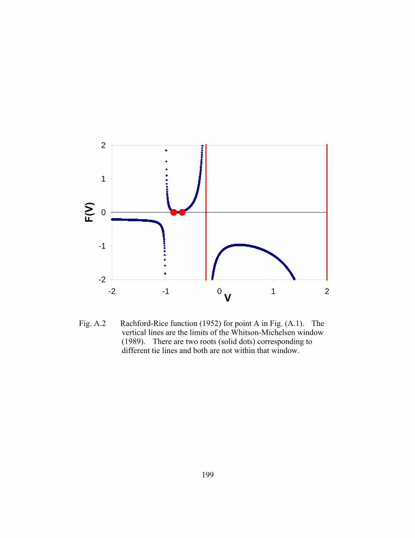
199
-2
-1
0
1
2
-2 -1 0 1 2V
F(V)
Fig. A.2 Rachford-Rice function (1952) for point A in Fig. (A.1). The vertical lines are the limits of the Whitson-Michelsen window (1989). There are two roots (solid dots) corresponding to different tie lines and both are not within that window.

200
-4
-2
0
2
4
0 0.05 0.1 0.15 0.2x1
F(x 1
)
New Method
Wang-Orr
Fig. A.3 Objective functions for point A in Fig. (A.1) based on the new objective method and that given by Wang and Orr (1997, 1998). The two correct roots (the solid dots) lie within the window given by Eq. (A.7). The new objective function is very linear.

201
-4
-2
0
2
4
-4 -2 0 2 4V
F(V)
Fig. A.4 Rachford-Rice function (1952) for point B in Fig. (A.1). The vertical lines are the limits of the Whitson-Michelsen window (1989). The correct root (solid dot) is not within the window.

202
-4
-2
0
2
4
0 0.05 0.1 0.15 0.2x1
F(x 1
)
New Method
Wang-Orr
Fig. A.5 Objective functions for point B in Fig. (A.1) based on the new objective method and that given by Wang and Orr (1997, 1998). The correct root (the solid dot) lies within the window given by Eq. (A.7). The new objective function is very linear.

203
Glossary
a attraction parameter for EOS, 3 /psia ft lbm mol⋅ −
A attraction parameter for EOS, dim.
b repulsion parameter for EOS, 3 /ft lb mol−
B repulsion parameter for EOS, dim.
C transformed composition, dim.
d dimensionless chemical potential, dim.
D dimensionless chemical potential, dim.
e error or objective function
F objective function
f component fugacities, psia
g binary interaction parameter for new model, see Eqs. (2.5), dim.
h binary interaction parameter for new model, see Eqs. (2.5), dim.
J Jacobian matrix, dim.
k binary interaction parameter, dim.
K K-value, dim.
L liquid mole fraction, dim.
NC number of components
NP number of phases
MW molecular weight, dim
P reservoir pressure, psia
q reduced variable for pure components, dim.
R gas constant, 3 /psia ft lb mol R⋅ − ⋅

204
T temperature, oF
V molar volume, 3 /ft lb mol−
V vapor mole fraction, dim.
x liquid phase molar composition, dim. *X transformed liquid phase molar comopsition, dim.
y vapor phase molar composition, dim.
y composition at the stationary point, dim.
Y modified primary variable in stability analysis *Y transformed vapor phase molar comopsition, dim.
Y modified stationary points in stability analysis
z overall composition, dim. *Z transformed overall molar comopsition, dim.
α transformation parameter,dim.
δ Kronecker delta function
1δ EOS parameter, see Eq. (2.3)
2δ EOS parameter, see Eq. (2.3) j
iφ component fugacity coefficient, dim.
Θ reduced parameters, various dimensions
ω acentric factor, dim.
μ chemical potential, J/mol
Superscripts and Subscripts
* transformed composition
i,j species index
k,l index for reduced parameters
c critical properties

205
D dimensionless quantity
j,l phase index
L liquid phase
m mixture property
max upper boundary of the investigation range
min lower boundary of the investigation range
ref reference component
T total property of multi-phase mixture
V vapor phase

206
Bibliography
Baker L.E., Pierce, A.C. and Luks, K.D.: “Gibbs Energy Analysis of Phase Equilibria,” SPEJ, 22: 731-742, 1982.
Bullard, L. G. and Biegler, L. T.: “Iterated Linear Programming Strategies for Non-smooth Simulation: a Penalty Based Method for Vapor-liquid Equilibrium Applications,” Comp. & Chem. Eng., 17 (1), 95-109, 1993.
Chang, Y.: “Development and Application of an Equation of State Compositional Simulator,” Ph.D. dissertation, the University of Texas at Austin, 1990.
Coats, K.H.: “ Simulation of Gas Condensate Reservoir Performance,” JPT, 1870-1886, 1985
Egwuenu, A.M., Johns, R.T., and Li, Y.: “Improved Fluid Characterization for Miscible Gas Floods,” SPE 94034 presented at 2005 SPE Europec Conference, Madrid, Spain, June 13-16.
Firoozabadi A. Thermodynamics of Hydrocarbon Reservoirs. New York, NY: McGraw-Hill; 1999.
Firoozabadi, A. and Pan, H.: “Fast and Robust Algorithm for Compositional Modeling: Part I: Stability Analysis Testing,” SPEJ (Mar 2002), 78-89.
Gautam, R. and Seider, W. D.: “Computation of Phase and Chemical Equilibrium. Part I. Local and Constrained Minima in Gibbs Free Energy,” AIChE J., 25: 991-999, 1979.
Han, G. And Rangaiah, G. P.: “ A Method for Calculation of Vapor-Liquid and Liquid-Liquid Equilibria,” Comp. & Chem. Eng., 21 (8): 905-/913, 1997.
Hand, D.B.: “ Dineric Distribution,” J.Phy.Chem., 34 (9): 1961-2000, 1930.
Harding S.T. and Floudas C.A.: “Phase Stability with Cubic Equations of State: A Global Optimization Approach,” AIChE J., 7:1422-1440, 2000.
Hearn, C.L and Whitson, C.H.: “Evaluating Miscible and Immiscible Gas Injection in the Safah Field, Oman,” SPE 29115 presented at the 1995 SPE Symposium on Reservoir Simulation, San Antonio, TX, Feb 12-15.
Heidemann, R. A. Three-phase Equilibria Using Equations of State. AIChE J., 20:847-855,1974.

207
Hendriks, E.M.: “Reduction Theorem for Phase Equilibrium Problems,” Ind.Eng.Chem.Res., 27:1728-1733, 1988.
Hendriks, E.M. and Van Bergen, A.R.D.: “Application of a Reduction Method to Phase Equilibria Calculations,” Fluid Phase Equilib., 74:17,1992.
Hong, K.C.: “Lumped-Component Characterization of Crude Oils for Compositional Simulation,” SPE 10691 presented at 1982 SPE/DOE Enhanced Oil Recovery Symposium, Tulsa, OK, Apr 4-7.
Hoteit, H. and Firoozabadi, A.: “ Simple Phase Stability-Testing Algorithm in the Reduction Method,” AIChE J., 52(8), 2909-2920, 2006.
Hua J.Z., Brennecke J.F., Stadtherr M.A.: “Reliable Prediction of Phase Stability Using an Interval Newton Method,” Fluid Phase Equilib., 116:52-59,1996.
Hua J.Z., Brennecke J.F., Stadtherr M.A.: “Reliable Computation of Phase Stability Using Interval Analysis: Cubic Equation of State Models,” Comput. Chem Eng., 22:1207-1214,1998
Jensen, B.H. and Fredenslund, A.: “A Simplified Flash Procedure for Multicomponent Mixtures Containing Hydrocarbons and One Non-hydrocarbon Using Two-parameter Cubic Equations of State,” Ind.Eng.Chem.Res., 26: 2129-2134,1987.
Jessen,K., Michelsen, M.L. and Stenby, E.H.: “Global Approach for Calculation of Minimum Miscibility Pressure,” Fluid Phase Equilibria., 153(2):251-263, 1998.
Johns, R.T., Dindoruk, B. and Orr, F.M. Jr.: “Analytical Theory of Combined Condensing/Vaporizing Gas Drives,” SPE Adv. Tech. Series, 1: 7-16, 1992.
Johns, R.T. and Orr, F.M. Jr.: “Miscible Gas Displacement of Multicomponent Oils,” SPEJ (Mar 1996), 39-46.
Johns, R.T., Fayers, F.J., and Orr, F.M. Jr.: “Effect of Gas Enrichment and Dispersion on Nearly Miscible Displacement in Condensing/Vaporizing Drives,” SPE Adv. Tech. Series, 2: 26-34, 1993.
Leibovici, C.F. and Neoschil, J.: “A Solution of Rachford-Rice Equation,” Fluid Phase Equilibria, 74(1): 303-308, 1992.
Leibovici, C.F. and Neoschil, J.: “A New Look at the Rachford-Rice Equations for Multiphase Systems,” Fluid Phase Equilibria, 112(2): 217-221, 1995.
Li, Y.K. and Nghiem, L.X.: “The Development of a General Phase Envelope Construction Algorithm for Reservoir Fluid Studies,” SPE 11198 presented at

208
1982 SPE Annual Technical Conference and Exhibition in New Orleans, LA, September 26-29.
Liu, K.: “Reduce the Number of Components for Compositional Reservoir Simulation,” SPE 66363 presented at the 2001 SPE Reservoir Simulation Symposium, Houston, TX, Feb 11-14.
Litvak, M.L. and Wang. C.H.: “Integrated Reservoir and Surface Pipeline Network Compositional Simulations,” SPE 48859 is presented at the 1998 SPE International Conference and Exhibition in Beijing, China, November 2-6.
McDonald CM, Floudas CA.: “Global Optimization for the Phase Stability Problem,” AIChE J., 41:1798-1814,1995
Michelsen, M.: “The Isothermal Flash Problem. Part I: Stability,” Fluid Phase Equilib., 9:1-19, 1982.
Michelsen, M.: “The Isothermal Flash Problem. Part II: Phase Split Calculation,” Fluid Phase Equilib., 9: 21-40, 1982.
Michelsen, M.: “Simplified Flash Calculation for Cubic Equations of State,” Ind.Eng.Chem.Proc.Des.Dev., 25: 184-188, 1986.
Monroy-Loperena, R. and Vargas-Villamil, F.D.: “On the Determination of the Polynomial Defining Vapor-Liquid Split of Multi-Component Mixtures,” Chem.Eng.Sci., 56(20): 5865-5868, 2001.
Nagarayan, N. R., Cullik, A. S. and Griewank, A.: “New Strategy for Phase Equilibrium and Critical Point Calculations by Thermodynamic Energy Analysis. Part I. Stability Analysis and Flash,” Fluid Phase Equilib., 62: 191-210,1991
Nichita, D.V.: “A Reduction Method for Phase Equilibrium Calculations with Cubic Equations of State,” Brazilian J. of Chemical Engineering, 23(3): 427-434, 2006
Nichita, D.V., Broseta, D., and Hemptinne, J.C.: “Multiphase Equilibrium Calculation Using Reduced Variables,” SPE 89439 presented at the 2004 SPE/DOE 14th Symposium on Improved Oil Recovery, Tulsa, OK, April 17-21.
Nichita, D. V., Broseta, D., de Hemptinne, J.-C. and Lachet, V.: “Efficient Phase Equilibrium Calculation for Compositional Simulation: the Direct Reduced Flash,” Petro. Sci. & Tech., 25(3): 315-342, 2007.
Nichita, D.V., De Los Angeles Duran Valencia, C. and Gomez, S.: “Volume-based Thermodynamics Global Phase Stability Analysis,” Chem. Eng. Comm., 193(10): 1194-1216, 2006.

209
Nichita, D.V., Gomez, S. and Luna, E.: “Multiphase Equilibria Calculation by Direct Minimization of Gibbs Free Energy with a Global Optimization Method,” Comp. & Chem. Eng., 26(12), 1703-1724, 2002.
Nichita, D.V., Gomez S. And Luna, E.: “Phase Stability Analysis with Cubic Equations of State by Using a Global Optimization Method,” Fluid Phase Equilib., 194: 411-437, 2002.
Nichita, D.V. and Minescu, F.: “Efficient Phase Equilibrium Calculation in a Reduced Flash Context,” Can. J. Chem. Eng., 82(6), 1225-1238, 2004.
Okuno, R. Private communications, 2007.
Pan, H. and Firoozabadi, A.: “Fast and Robust Algorithm for Compositional Modeling: Part II: Two-phase Flash Computations,” SPE 71603 presented at 2001 ATCE, New Orleans, LA, September 30 – October 3.
Peng, D.Y. and Robinson, D.B.: “A Rigorous Method for Prediction the Critical Properties of Multicomponent Systems from an Equation of State,” AIChEJ, 23: 137, 1977.
Pope, G.A., Tsaur, K, Schechter, R.S. and Wang, B: “The Effect of Several Polymers on the Phase Behavior of Micellar Fluids,” SPEJ, 1982 Dec, 816-830.
Rachford, H.H. and Rice, J.D.: “Procedure for Use of Electronic Digital Computers in Calculating Flash Vaporization Hydrocarbon Equilibrium,” Petroleum Transactions AIME, 195: 237-238, 1952.
Rasmussen C.P., Krejbjerg K., Michelsen M.L. and Bjurstrom K.E.: “Increasing Computational Speed of Flash Calculations with Application for Compositional, Transient Simulations,” SPERE, 2006 February, 32-38.
Redlich, O., and Kwong, J.S.: “On the Thermodynamics of Solutions. V: An Equation of State. Fugacities of Gaseous Solutions, “ Chem. Rev., 44: 233, 1949.
Soave, G.: “Equilibrium Constants from a Modified Redlich-Kwong Equation of State,” Chem. Eng. Sci. , 27: 1197, 1972.
Solano, R., Johns, R.T., and Lake, L.W.: “Impact of Reservoir Mixing on Recovery in Enriched-Gas Drives Above the Minimum Miscibility Enrichment,” SPEREE, 4(5), 358-365, 2001.
Stenby, E.H. and Wang, P.: “Noniterative Phase Equilibrium Calculation in Compositional Reservoir Simulation,” SPE 26641 presented at 1993 ATCE, Houston, TX, October 3-8.

210
Sun A.C. and Seider W.D..: “Homotopy-continuation Method for Stability Analysis in the Global Minimization of the Gibbs Free Energy,” Fluid Phase Equilib., 103: 213-249, 1995.
Tang, D.E. and Zick, A.A.: “A New Limited Compositional Reservoir Simulator,” SPE 25255 presented at 1993 SPE Symposium on Reservoir Simulation, New Orleans, LA, February 28 – March 3.
Trangenstein, J.A.: “Minimization of Gibbs Free Energy in Compositional Reservoir Simulation”, paper SPE 13520, presented at the SPE 1985 Reservoir Simulation Symposium, Dallas, TX.
Von Rossenberg, D.U.: “Determination of the Polynomial Defining Vapor-Liquid Split of Multi-Component Mixtures,” Chem. Eng. Sci., 18(4): 219-222, 1963.
Von Rossenberg, D.U.: “On the Determination of the Polynomial Defining Vapor-Liquid Split,” Chem.Eng.Sci., 32(12): 1546-1547, 1977.
Voskov, D.V. and Tchelepi,H.A.: “Compositional Space Parameterization for Flow Simulation,” SPE 106029 presented at 2007 SPE Reservoir Simulation Symposium, Houston, TX, February 26-28.
Wang, Y. and Orr, F.M. Jr.: “Calculation of Minimum Miscibility Pressure,” SPE 29683 presented at 1998 SPE/DOE Improved Oil Recovery Symposium, Tulsa, OK, April 19-22.
Wang, Y. and Orr, F.M. Jr.: “Analytical Calculation of Minimum Miscibility Pressure,” Fluid Phase Equilib., 139(1):101-124, 1997.
Warren, J.H. and Adewumi, M.A.: “Polynomial Objective Fucntions for Flash Calculations: Binary, Ternary and Quaternary Systems,” Ind.Eng.Chem.Res., 32(7), 1528-1530, 1993.
Whitson, C.H. and Michelsen, M.L.: “The Negative Flash,” Fluid Phase Equilib., 53(1): 51-71, 1989.
Yuan, H. and Johns, R.T.: “Simplified Method for Calculation of Minimum Miscibility Pressure or Enrichment,” SPEJ, December 2005: 416-425.
Zick, A.A.: “A Combined Condensing/Vaporizing Mechanism in the Displacement of Oil by Enriched Gases,” SPE 15493 presented at 1986 ATCE, New Orleans, LA, October 5-8.

211
Vita
Yinghui Li was born on September 27, 1976 in Handan, Hebei province, China,
the son of Qi Li and Naibo Liu. In 1994, he entered Tsinghua University in Beijing,
China, and received the degree of Bachelor of Science in Chemical Engineering in 1999
in this five-year program. In the same year, he was admitted to Chinese Academy of
Science Graduate School in Beijing for a three-year graduate program in Chemical
Engineering in the Institute of Process Engineering. He received a Master of Science
degree in 2002, and then entered the Department of Petroleum and Geosystems
Engineering at the University of Texas at Austin in 2003. He has authored and co-
authored three SPE papers. He was awarded Pre-emptive Fellowship in 2003 and
Conoco-Phillips Fellowship in 2004.
Permanent address: 1624 W 6th Street, Apt M, Austin, TX, 78703
This dissertation was typed by Yinghui Li.