Embed Size (px)
Citation preview


©Copyright by Willard Lawrence Quon 2012
All Rights Reserved

A Compact and Efficient Steam Methane Reformer for
Hydrogen Production
A Dissertation
Presented to
The Faculty of the Department of Chemical and Biomolecular Engineering
University of Houston
In Partial Fulfillment
of the Requirements for the Degree
Doctor of Philosophy
in Chemical Engineering
by
Willard Lawrence Quon
August 2012

A Compact and Efficient Steam Methane
Reformer for Hydrogen Production
________________________________ Willard Lawrence Quon
Approved: ____________________________________
Chairman of the Committee
James. T. Richardson, Professor Emeritus,
Chemical and Biomolecular Engineering
Committee Members: ____________________________________
Michael P. Harold, M. D. Anderson
Professor, Chemical and Biomolecular
Engineering
____________________________________
Allan J. Jacobson, Robert A. Welch Chair of
Science, Director of the Texas Center for
Superconductivity at UH
____________________________________
William S. Epling, Associate Professor,
Chemical and Biomolecular Engineering
____________________________________
William Rixey, Associate Professor,
Civil and Environmental Engineering
____________________________________
Micky Fleischer, Adjunct Professor,
Chemical and Biomolecular Engineering
____________________________ ____________________________________
Suresh K. Khator, Associate Dean Ramanan Krishnamoorti, Dow Chair
Cullen College of Engineering Professor and Department Chair,
Chemical and Biomolecular Engineering

v
Acknowledgements
As the end of this long effort approaches, many feelings arise; relief being on the
threshold of completion of this long journey, appreciation for all those who assisted me
along the way, and optimism for what the future holds as I apply what I learned from this
experience in my career. I would like to thank all the individuals who have helped me
accomplish this goal.
To begin, it has been both a great privilege and opportunity to work for, and with,
Dr. James T. Richardson, my advisor; His depth of knowledge in his field, and
dedication to research and teaching has set an excellent example and is an inspiration for
me to follow; his patience and guidance, in spite of missed meetings caused by numerous
other demands on my time by my full-time day job has provided the continuity along the
way that has allowed me to progress towards completion of this journey. He has always
provided encouragement toward this ultimate goal, and we have even shared non-
academic discussions as well, ranging from computers to local politics. He is a very
approachable mentor, and is an example of knowledge, professionalism, and humanity,
that is a worthy role model for me to follow.
I would also like to express my gratitude to the following people: Dr. Allan
Jacobson, Dr. Michael Harold, Dr. William Rixey, Dr. Miguel Fleischer, and Dr. William
Epling for serving on my dissertation committee and for their comments and suggestions.
Additional thanks go to my fellow graduate student, Geofrey Goldwin Jeba, who was a
willing sound-board for ideas, and who also helped validate the dimensionless heat and
mass transfer equations used in our studies together.

vi
I would be remiss if I did not acknowledge the contributions of people who paved
the way and provided the initial encouragement to embark on this journey. First is my
wife Fern, whose quest for lifelong learning has been the single most important example
and influence on my academic career. I have been truly blessed to have been married to
this human dynamo for 35 years. Next, my managers at Du Pont, Philip Anderson and
Allen Webb, were ardent supporters of mine. Without their special dispensations in the
form of flexible work schedules, I would have had a much harder time getting the first
two years of classes completed, and may have gotten too discouraged to continue.
Another colleague at Du Pont, Dr. Ross C. Koile, was also a positive influence and
supporter. Lastly, I would like to thank my managers at Invista S.A.R.L., Grant R.
Pittman and Lori Cordray, for their patience and support.
vii
A Compact and Efficient Steam Methane Reformer for
Hydrogen Production
An Abstract
of a
Dissertation
Presented to
The Faculty of the Department of Chemical and Biomolecular Engineering
University of Houston
In Partial Fulfillment
of the Requirements for the Degree
Doctor of Philosophy
in Chemical Engineering
by
Willard Lawrence Quon
August 2012

viii
Abstract
A small-scale steam-methane reforming system for localized, distributed
production of hydrogen offers improved performance and lower cost by integrating the
following technologies developed at the University of Houston;
(1) Catalyzed steam-methane reforming on ceramic foam catalyst substrates.
(2) Coupling of reformers to remote heat sources via heat pipes instead of heating by
direct-fired heaters.
(3) Catalytic combustion of methane with air on ceramic foam substrates as the heat
source.
Each of these three technologies confer benefits improving the efficiency, reliability, or
cost of an integrated compact steam-methane reforming system.
A prior 2-D computer model was adapted from existing FORTRAN code for a
packed-bed reactor and successfully updated to better reflect heat transfer in the ceramic
foam bed and at the reactor wall, then validated with experimental heat transfer and
reaction data for use in designing commercial-scale ceramic foam catalytic reactors.
Different configurations and sizes of both reformer and combustor reactors were studied
to arrive at a best configuration for an integrated system. The radial and axial
conversions and temperatures of each reactor were studied to match the heat recovery
capability of the reformer to the heat generation characteristics of the combustor.
The vetted computer model was used to size and specify a 500 kg/day hydrogen
production unit featuring ceramic foam catalyst beds integrated into heat pipe reactors
that can be used for multiple end users, ranging from small edible fats and oils
hydrogenators to consumer point of sale hydrogen fueling stations. The estimated
ix
investment for this 500 kg/day system is $2,286,069 but is expected to drop to less than
$1,048,000 using mass production methods.
Economic analysis of the 500 kg/day hydrogen production system shows that it is
not presently competitive with gasoline as a transportation fuel, but the system is still
economically attractive to stationary fuel cell applications or small chemical users with a
delivered hydrogen price as low as $1.49/kg, even with a 10% IRR that includes
investment recovery, depreciation, taxes, etc.
x
Table of Contents
Acknowledgments v
Abstract vii
Table of contents x
List of Figures xvii
List of Tables xxiii
Nomenclature xxvi
Chapter One: Introduction and goal of this Study 1
1.1 Hydrogen manufacturing processes 2
1.2 Hydrogen markets 5
1.2.1 Present industrial production and usage 5
1.2.2 Transportation fuel 10
1.2.3 Stationary power 11
1.2.4 Other uses 12
1.3 Supply strategies to develop hydrogen as a transportation fuel 13
1.3.1 Mobile on-board hydrogen generation 14
1.3.2 Centralized hydrogen production 15
1.3.3 Distributed hydrogen production 20
1.3.4 Phase-wise distributed to centralized evolution 22
1.4 Incentives for current research 25
Chapter Two Background: Steam methane reforming, heat pipes,
ceramic foam reactors, catalytic
combustion, and prior studies 26
2.1 Introduction 26
xi
2.2 Steam methane reforming 26
2.2.1 Chemistry and Thermodynamics 28
2.2.2 Catalysts 31
2.2.3 Pretreatment 32
2.3 Steam methane reforming reaction parameters 33
2.3.1 Reactant concentration: Steam to methane ratio 33
2.3.2 Reformer temperature 33
2.3.3 Pressure 34
2.4 Design of current commercial reformers 35
2.4.1 Tube and catalyst pellet geometry 35
2.4.2 Materials of construction 38
2.4.3 Furnace configuration and burner arrangements 40
2.5 Operating conditions 42
2.5.1 Prevention of carbon fouling 43
2.5.2 Prevention of hot spots or hot bands 44
2.5.3 Reformer tube life 45
2.5.4 Gas flow distribution 47
2.5.5 Thermal efficiency 48
2.5.6 Summary of operating conditions 49
2.6 Small scale SMR reformer systems 49
2.6.1 Disadvantages of current SMR technology at small scales 50
2.6.2 Desired characteristics of small-scale reformers 55
2.7 Hydrogen production research at the University of Houston 57

xii
2.8 Heat pipes 57
2.8.1 Advantages of heat pipes 59
2.8.2 Choice of working fluid 61
2.8.3 Limitations 63
2.8.4 Safety considerations of the working fluid 67
2.8.5 Prior heat pipe studies at the University of Houston 71
2.9 Ceramic foam catalyst supports 76
2.9.1 Heat transfer improvement 80
2.9.2 Pressure drop improvement 83
2.9.3 Mass transfer improvement 84
2.10 Catalytic combustion 85
2.10.1 New high durability catalysts 88
2.11 Summary of background and objectives of the current research 89
Chapter Three: Reactor simulation models 91
3.1 Introduction 91
3.2 Two-dimensional catalytic reactor basic equations 91
3.2.1 Mass balance 93
3.2.2 Energy balance 96
3.2.3 Discretization of the mass and energy balances 98
3.2.4 Step sizes for the numerical integration 101
3.2.5 Parameter inputs 101
3.3 Heat transfer modeling: thermal resistances and conductivities 102
3.4 Excel™ Model 107

xiii
3.4.1 Excel™ interface 108
3.4.2 VBA interface 110
3.5 Determining heat transfer correlations of 30 PPI α-Al2O3 ceramic foam 111
3.6 Validation of the computer model, heat transfer only 113
3.6.1 Model upgrades 114
3.6.2 Radial temperature profiles without reaction 116
3.6.3 Axial temperature profiles without reaction 123
3.6.4 Heat transfer conclusions 131
3.7 Validation of the computer model, methane catalytic combustion 131
3.8 Parametric studies of the model 134
3.8.1 Operating pressure 136
3.8.2 Heat pipe wall temperature 139
3.8.3 Gas inlet temperature 142
3.8.4 Reactor feed rates 144
3.8.5 Reactor diameter 147
3.8.6 Pre-exponential constant 149
3.8.7 Summary of combustor parametric evaluation 151
3.9 Parametric studies of the reformer model 153
3.9.1 Reforming reaction 153
3.9.2 Operating pressure 154
3.9.3 Heat pipe wall temperature 156
3.9.4 Gas inlet temperature 157
3.9.5 Reactor feed rates 158
xiv
3.9.6 Reactor diameter 160
3.9.7 Pre-exponential constant 161
3.9.8 Summary of reformer parametric evaluation 162
Chapter Four: Reactor model optimization 165
4.1 Combustor 165
4.1.1 Heat output 165
4.1.2 Conversion 170
4.1.3 Emissions 171
4.1.4 Service Life 174
4.1.5 Combustor summary 174
4.2 Reformer 175
4.2.1 Reformer sizing 175
4.2.2 Conversion 176
4.2.3 Reformer summary 177
Chapter Five: Integrated steam-methane reformer hydrogen plants 178
5.1 Introduction 178
5.2 Heat pipe reactors 178
5.3 Ceramic foam catalyst support selection 181
5.4 Reformer and reformer combinations 181
5.5 Summary and recommended configuration 183
5.5.1 Sizing basis 184
5.5.2 Combustor 184
5.5.3 Reformer 186

xv
5.5.4 Heat Pipe 189
5.5.5 Energy balance 189
5.5.6 Safety considerations in design 190
Chapter Six: Integrated system 192
6.1 Introduction 192
6.1.1 Performance targets 192
6.1.2 Integrated flow sheet 192
6.1.3 Heat balance 194
6.1.4 Energy efficiency 198
6.2 System components and estimated costs 199
6.2.1 Reformer and combustor reactor 199
6.2.2 Heat Exchangers 200
6.2.3 Hydrogen purification 203
6.2.4 Overall cost of an integrated system 204
6.2.5 Impact of the experience curve on system cost 204
6.3 Cost Comparison with competing hydrogen technologies 206
6.3.1 Conventional steam methane reforming 206
6.3.2 Electrolysis 208
6.4 U.S. Department of Energy H2A program 209
6.4.1 H2A cases studied 212
6.4.2 High investment high natural gas price case 213
6.4.3 High investment low natural gas price case 213
6.4.4 Low investment high natural gas price case 214

xvi
6.4.5 Low investment low natural gas price case 214
6.4.6 Summary of H2A cases 215
6.5 Chapter summary 216
6.5.1 Fueling station applications 216
6.5.2 Small scale applications 217
Chapter Seven: Conclusions and recommendations 218
7.1 Conclusions 218
7.2 Recommendations for future work 220
References 221
Appendices 233
Appendix 1 – Reformer VBA program listing 234
Appendix 2 – Combustor VBA program listing 279
Appendix 3 – Computer simulation results versus lab tests (radial profiles) 337
Appendix 4 – Computer simulation results versus lab tests with confidence 346
limits (radial profiles)
Appendix 5 – Computer simulation results versus lab tests (axial profiles) 380
Appendix 6 – U.S. Department of Energy H2A input sheet 397
xvii
List of Figures
Figure 1-1 - Hydrogen production routes source – U.S. Department of
Energy (EERE) -2010 [7] 3
Figure 1-2 - Schematic of a typical hydrogen plant using steam reforming. 4
Figure 1-3 - 2009 US annual production of key basic chemicals 6
(million annual metric tons)
Figure 1-4 - 2011 US split of hydrogen production among markets [11] 7
Figure 1-5 - Optimum hydrogen delivery modes by distance and volume [16] 8
Figure 1-6 - Map of United States industrial hydrogen production facilities [17] 9
Figure 1-7 - Gaseous hydrogen delivery pathway [28] 16
Figure 1-8 - Cryogenic liquid hydrogen delivery [28] 17
Figure 1-9 - Alternative carrier hydrogen delivery [28] 19
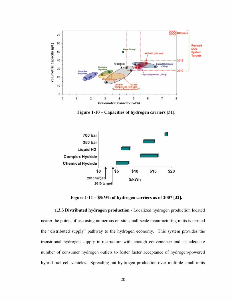
Figure 1-10 - Capacities of hydrogen carriers [31] 20
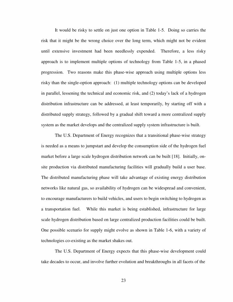
Figure 1-11 - $/kWh of hydrogen carriers as of 2007 [32] 20
Figure 1-12 – Comparison of fuel pathways regarding emissions and costs [33] 21
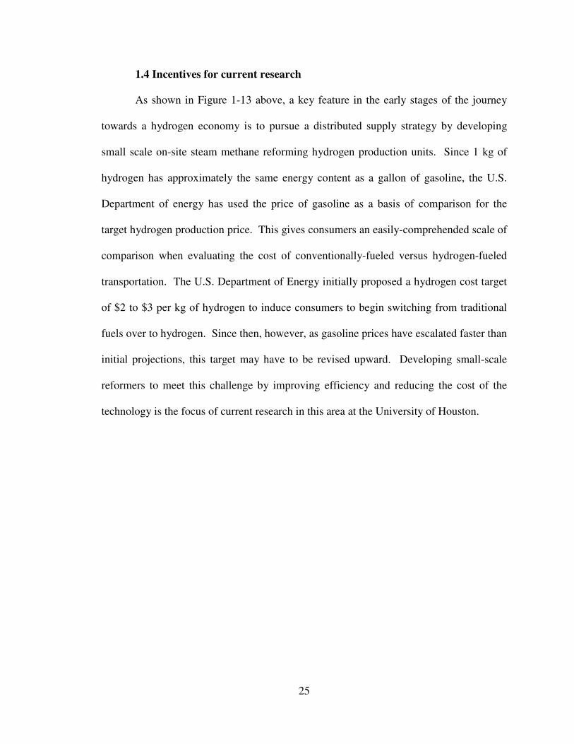
Figure 1-13 - Possible evolution of hydrogen technologies [6] 24
Figure 2-1 - Schematic of a typical hydrogen plant using steam reforming [8] 27
Figure 2-2 - Equilibrium percentage of CH4 after reforming [35] 30
Figure 2-3 - Equilibrium conversions for steam methane reforming [36] 31
Figure 2-4 - Catalytic metals used for steam methane reforming [36] 31
Figure 2-5 - Typical reactor tube for steam methane reforming 35
Figure 2-6 - Relative Pressure drop vs. catalyst pellet size [37] 36
Figure 2-7 - Typical steam methane reformer tube axial temperature profile 38
Figure 2-8 - Typical configurations of reformer furnaces: (a) bottom fired,
(b) top fired, (c) terrace wall, (d) side fired [36] 42
xviii
Figure 2-9 - Typical terrace wall reformer furnace [35] 43
Figure 2-10 - Abnormal thermal images of reformer tubes [36] 45
Figure 2-11 - Larson-Miller parameter results of 170 tube rupture tests [35] 46
Figure 2-12 - Reformer tube life [35] 47
Figure 2-13 - Conventional design for small scale steam methane reformers [38] 50
Figure 2-14 - Production costs per Nm3 of hydrogen vs. plant capacity [8] 52
Figure 2-15 - Schematic of a typical heat pipe showing the principle of
operation and circulation of the working fluid [40] 58
Figure 2-16 - Heat flux for sodium evaporation from a compound wick vs.
critical heat flux for pool boiling (Ivanoskii 1982) [41] 59
Figure 2-17 - Comparison of theoretical heat transport limits with experimental
data (Faghri) [40] 65
Figure 2-18 - Pressure Balance in a Heat Pipe [40] 67
Figure 2-19 - Predicted heat-pipe temperature rise versus measured [46,47] 70
Figure 2-20 - Theoretical heat-pipe temperature rise versus steam injection
pressure [46,47] 71
Figure 2-21 - Heat pipe layout showing flow of heat (Richardson, et al.) [49] 73
Figure 2-22 - Hydrogen permeation into the pilot plant heat pipe (Shen) [51] 73
Figure 2-23 - Gas-fired heat pipe reformer 75
Figure 2-24 - 20 kW Sandia-Israel reflux heat-pipe receiver/reactor [48] 76
Figure 2-25 - Steps for making a ceramic foam substrate [36] 77
Figure 2-26 - Varietal shapes for ceramic foam substrates [36] 78
Figure 2-27 - Photomicrograph of a reticulated ceramic foam [36] 78
Figure 2-28 - Wash-coat applied to a ceramic foam surface [36] 79
Figure 2-29 - Nusselt number of 30 PPI Ceramic Foam vs. spherical catalyst
supports [36] 81

xix
Figure 2-30 - Comparison of pressure drop for a bed of glass spheres and 30-PPI,
99.5 wt.% α-Al2O3 [53] 83
Figure 2-31 - Colburn plot of jD versus Res [55] 84
Figure 2-32 - Reformer firebox geometry and internal temperature contours [63] 86
Figure 2-33 - Effect of combustion temperature on oxides of nitrogen creation [36] 87
Figure 2-34 - Typical catalytic combustor reactor average axial temperature
profile 88
Figure 3-1 - Annular heat pipe reactor surrounding an internal heat pipe 92
Figure 3-2 - Cylindrical heat pipe reactor inside an external heat pipe 93
Figure 3-3 - Differential element of the catalyst bed. 93
Figure 3-4 - Axial flow cylindrical ceramic foam reactor radii for heat transfer
coefficients 106
Figure 3-5 - Reactor parameter input sheet 109
Figure 3-6 - Physical property parameter input sheet 109
Figure 3-7 - Example VBA IDE Screen 110
Figure 3-8 - Schematic of thermocouple locations in the laboratory ceramic bed 112
Figure 3-9 - Radial temperature profiles – model versus Peng data set 3 [57] 114
Figure 3-10 - Radial temperature profiles – computer model versus Peng lab
data, with modified KEFF and HCVHP [57] 116
Figure 3-11 - Computer simulation results versus lab test number 1 117
Figure 3-12 - Model predicted radial temperature profile versus lab test #1
at l/L = 0.167 with confidence limits 119
Figure 3-13 - Lab Axial Temperatures versus Computer Model for all 17 Runs 125
Figure 3-14 - Axial temperature profile for run 5 (lab and computer prediction) 126
Figure 3-15 - Run 5 lab versus computer predicted axial temperatures 127
xx
Figure 3-16 - Laboratory external shell temperature profiles (run 5 is highlighted) 128
Figure 3-17 - Feed rates versus inlet temperatures (run 5 is highlighted) 128
Figure 3-18 - Axial temperature profile for run 6 (lab and computer prediction) 129
Figure 3-19 - Axial centerline computer simulation results versus lab test
number 1 130
Figure 3-20 - Laboratory external shell temperature profiles (Runs 1-4
highlighted) 130
Figure 3-21 - Lab reactor for testing ceramic foam combustor 132
Figure 3-22 - Computer predictions of the combustor conversion vs.
actual lab data 133
Figure 3-23 - Combustor conversion profile vs. pressure, P 137
Figure 3-24 - Combustor axial temperature profile vs. pressure, P 138
Figure 3-25 - Combustor local peak temperature vs. pressure, P 139
Figure 3-26 - Combustor conversion profile vs. heat pipe wall temperature, THP 140
Figure 3-27 - Combustor axial temperature profile vs. heat pipe wall
temperature, THP 141
Figure 3-28 - Combustor local peak temperature vs. reactor wall temperature, THP 141
Figure 3-29 - Combustor conversion profile vs. gas inlet temperature, Tin 142
Figure 3-30 - Combustor axial temperature profile vs. gas inlet temperature, Tin 143
Figure 3-31 - Combustor local peak temperature vs. inlet temperature, Tin 144
Figure 3-32 - Combustor conversion profile vs. feed rate, F 145
Figure 3-33 - Combustor axial temperature profile vs. reactor feed rate, F 145
Figure 3-34 - Combustor local peak temperature vs. reactor feed rate, F 146
Figure 3-35 - Combustor conversion profile vs. reactor diameter, D 147
Figure 3-36 - Combustor axial temperature profile vs. reactor diameter, D 149

xxi
Figure 3-37 - Combustor local peak temperature vs. reactor diameter, D 149
Figure 3-38 - Combustor conversion profile vs. k0 150
Figure 3-39 - Combustor axial temperature profile vs. k0 150
Figure 3-40 - Combustor local peak temperature vs. k0 151
Figure 3-41 - Reformer conversion profile vs. pressure, P 155
Figure 3-42 - Reformer axial temperature profile vs. pressure, P 156
Figure 3-43 - Reformer axial temperature profile vs. pressure, P (last 30%) 156
Figure 3-44 - Reformer conversion profile vs. heat pipe wall temperature, THP 157
Figure 3-45 - Reformer axial temperature profile vs. heat pipe wall
temperature, THP 157
Figure 3-46 - Reformer conversion profile vs. gas inlet temperature, Tin 158
Figure 3-47 - Reformer axial temperature profile vs. gas inlet temperature, Tin 158
Figure 3-48 - Reformer conversion profile vs. feed rate, F 159
Figure 3-49 - Reformer axial temperature profile vs. reactor feed rate, F 159
Figure 3-50 - Reformer conversion profile vs. reactor diameter, D 160
Figure 3-51 - Reformer axial temperature profile vs. reactor diameter, D 161
Figure 3-52 - Reformer conversion profile vs. k0 161
Figure 3-53 - Reformer axial temperature profile vs. k0 162
Figure 4-1 - Average axial temperature for the short ( 34.4 cm) combustor 169
Figure 4-2 - Average axial temperature for the long (100 cm) combustor 170
Figure 4-3 - Axial conversion profile for the long (100 cm) combustor 171
Figure 4-4 - Axial temperature profiles at different radial distances for the
combustor 173
Figure 4-5 - Radial NOx concentration profile for the heat pipe combustor 173

xxii
Figure 4-6 - Conversion profile of the reformer 177
Figure 5-1 - Single tube heat pipe reformer reactor [51] 178
Figure 5-2 - Multiple tube heat pipe reformer reactor [36] 179
Figure 5-3 - Reformers driven by (a) gas, or (b) catalytic combustion 182
Figure 5-4 - Reformer/Combustor combinations (a) concentric, or
(b) end to end 182
Figure 5-5 - Radial temperature profile versus z* distance for the combustor 186
Figure 5-6 - Average axial temperature profile versus z* distance for the reformer 188
Figure 5-7 - Radial temperature profile versus z* distance for the reformer 188
Figure 6-1 - Integrated steam methane reformer / catalytic combustor
hydrogen plant 193
Figure 6-2 - SMR H2 plant ASPEN™ Plus™ process simulation flowsheet 196
Figure 6-3 - SMR H2 plant heat duty by heat exchanger 197
Figure 6-4 - E-1 shell count by graphical solution 198
Figure 6-5 - E-1 shell count by graphical solution - expanded scale 198
Figure 6-6 - Combination reformer/heat pipe/combustor system (not to scale) 201
Figure 6-7 - Heat exchanger evaluation summary page for E-1 202
Figure 6-8 - Heat exchanger price to size correlation 203
Figure 6-9 - Experience curve for small hydrogen reforming systems 206
Figure 6-10 – Conventional steam methane reforming plant cost versus scale [38] 207
Figure 6-11 - U.S. DOE H2A model architecture [80] 209
Figure 6-12 - U.S. natural gas futures prices [82] 212

xxiii
List of Tables
Table 1-1 - 2003 United States and world hydrogen consumptions by
end-use [12] 6
Table 1-2 - Miles of U.S. gathering, transmission, and distribution
pipelines [14-15] 7
Table 1-3 - 2003 United States annual hydrogen consumptions by end-use [12] 10
Table 1-4 - Stationary power systems installed in the U.S. by December 2008 [20] 12
Table 1-5 - Other options to produce 40 million annual tons of hydrogen [18] 22
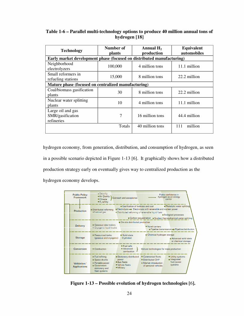
Table 1-6 - Parallel multi-technology options to produce 40 million annual tons
of hydrogen [18] 24
Table 2-1 - Reforming /water gas shift reaction features 29
Table 2-2 - Composition of HK 40 high temperature alloy [SFSA, 2004] 39
Table 2-3 - Nominal composition of Manaurite®
36X high temperature alloy
[Rolled Alloys, 2012] 39
Table 2-4 - Typical operating parameters for a SMR system 49
Table 2-5 - $/kW of SMR plant investment versus hydrogen output (2002) [38] 52
Table 2-6 - Heat pipe working fluid temperature ranges (Thermacore, Inc.) [28] 63
Table 2-7 - Energy released and temperature rise for water intrusion into sodium
heat pipes [46,47] 70
Table 2-8 - Properties of ceramic foam supports, 92% α-Al2O3, 18% mullite,
without washcoat [36] 79
Table 2-9 - Comparison of Thermal Parameters of Catalyst Support
Structures [36] 82
Table 2-10 - Methane catalytic combustion kinetic parameters on ceramic
foam [58] 89
Table 3-1 - Model parameter testing to resolve high thermal resistance at the wall 115
Table 3-2 - Comparison of computer predictions with lab data 120

xxiv
Table 3-3 - Comparison of computer model heat transfer coefficients 122
Table 3-4 - Comparison of axial centerline laboratory reactor temps
versus computer simulation results (no reaction present) 124
Table 3-5 - Correlation equation* and correlation coefficients for the computer-
predicted temperatures versus the Peng lab data 126
Table 3-6 - Laboratory experimental data with catalytic methane combustion 132
Table 3-7 - Laboratory experimental conversion vs. computer model predictions 133
Table 3-8 - Variables studied in the current model versus the Cantu study 135
Table 3-9 - Summary of the variables studied in the combustor parametric study 151
Table 3-10 – Ceramic foam physical properties 154
Table 3-11 - Summary of the variables studied in the reformer parametric study 162
Table 4-1 - Energy balance for integrated combustor/heat pipe/reformer 170
Table 4-2 - Expected NOx concentration as a function of gas temperature 172
Table 4-3 - Computer model evaluation of 15.24 cm diameter reformer 176
Table 5-1 - Energy balance for integrated combustor/heat pipe/reformer 189
Table 6-1 - Mass balance for the steam methane reformer / catalytic combustor
hydrogen plant of Figure 6-1 195
Table 6-2 - Temperatures for the integrated H2 plant 197
Table 6-3 - Heat exchanger sizes and prices 203
Table 6-4 - Major equipment costs for SMR H2 plant 204
Table 6-5 - Conventional steam methane reforming plant costs versus scale [38] 207
Table 6-6 - Conventional steam methane reforming plant costs in Shanghai [78] 208
Table 6-7 - Price of electrolytically-derived hydrogen [81] 208
Table 6-8 - U.S. DOE H2A model portion of input screen 211
Table 6-9 - Energy prices in the H2A version 3 model 212

xxv
Table 6-10 - H2A H2 delivered cost for high capital and high natural gas 213
Table 6-11 - H2A H2 delivered cost for high capital and low natural gas 214
Table 6-12 - H2A H2 delivered cost for low capital and high natural gas 214
Table 6-13 - H2A H2 delivered cost for low capital and low natural gas 215
Table 6-14 - H2A H2 delivered cost by capital and by natural gas price
at 10% IRR 215
Table 6-15 - H2A H2 delivered cost by capital and by natural gas price
at 7.5% IRR 216
Table 6-16 - H2A H2 delivered cost by capital and by natural gas price
at 5% IRR 216
Table 6-17 – H2A H2 delivered cost ex compression, storage, and dispensing 216

xxvi
Nomenclature
Cp Heat capacity (J mol-1
K-1
)
Deff Effective diffusivity (cm2sec
-1)
Der Mass diffusivity in the radial direction
Dp Particle diameter or foam pore diameter (cm)
F Reactor gas feed rate (SLPM)
G Superficial gas velocity (kg m-2
s-1
)
keff Effective thermal conductivity of the bed (W m-2
K-1
)
Nu Nusselt number
Pr Prandtl number
r radial position in the bed (cm)
r* dimensionless radial position in the bed
Re Reynolds number based on external surface area per volume of bed
ReS
Reynolds number based on external surface area per volume of solid
Sv External surface area per volume of solid ( cm2·cm
-3 )
T Temperature (ºK or ºC)
THP Heat pipe wall temperature (ºK)
Tin Inlet temperature (ºC)
v Axial gas velocity ( m·sec-1
)
z Axial bed position (m)
z* Dimensionless axial bed position
xxvii
Greek Letters
ε Foam porosity or packed bed void fraction
λg Thermal conductivity of the gas (W m-1
K-1
)
µ Gas viscosity (kgm−1
s−1
)
ρ Gas density (kg/m3
)
Acronyms used in the computer model
DR Radial incremental distance
DZ Axial incremental distance
HC Heat pipe conductive heat transfer coefficient through the wall
HCVHP Heat pipe convective heat transfer coefficient
HHP Sum of the heat pipe convective heat transfer coefficient (HCVHP) and
the radiative heat pipe heat transfer coefficient (HRHP)
HRHP Heat pipe radiative heat transfer coefficient
IDE Integrated development environment
KEFF Effective heat transfer coefficient
LEL Lower explosive limit
PPI Pores per inch
ppmvw parts per million by volume, wet basis
SLPM Standard liters per minute
UHP Heat pipe overall heat transfer coefficient
VBA Visual BASIC for Applications (Microsoft)
1
CHAPTER ONE
Introduction and goal of this study
Hydrogen is a versatile chemical in high demand for multiple industrial uses
around the world. The largest share of global hydrogen production is used in the
production of ammonia-based fertilizer for crops to feed the growing world population.
The next highest usage of hydrogen is in the energy arena for upgrading petroleum feed
stocks, thereby significantly improving the yield of usable fossil fuel to satisfy the rapidly
expanding energy demand [1]. However, the world’s growing consumption rate of fossil
energy has led to depletion of non-renewable reserves, and adverse impacts on the global
atmospheric environment in the form of greenhouse gas emissions, creating a need for
alternative clean energy sources [2].
Hydrogen has been proposed as a clean fuel for transportation and stationary
energy uses, since its consumption releases only water vapor instead of greenhouse gases
[3]. However, hydrogen is not a primary energy source and is merely an energy carrier,
since it is not readily available naturally. Rather, hydrogen must be produced from
another primary energy source, be it renewable, like solar, wind, or biomass, or other
non-renewables or fossil fuels such as coal or natural gas. Hydrogen can also be
produced from nuclear energy via electrolysis [4]. The degree of benefit gained from
using hydrogen as an energy carrier is a function of the primary energy source used to
make it and the measures taken to minimize greenhouse gases during hydrogen
production.
The long-term vision of widespread implementation of hydrogen as a universal
fuel is termed the “Hydrogen Economy.” However, the pathway to achieve full
2
acceptance of hydrogen as a fuel requires development of extensive distribution
infrastructure on the supply side, while on the demand side, consumer acceptance and
confidence that hydrogen is the future fuel of choice for both fixed and transportation
needs must be cultivated. The development of the “Hydrogen Economy” could take
decades. Until a large-scale hydrogen distribution infrastructure is built, a strategy to
assist in accelerating the demand side consumer acceptance of hydrogen fuel near-term is
to build a distributed hydrogen supply system based on small hydrogen-producing steam
methane reforming units [5]. Such units could take advantage of the extensive existing
natural gas distribution infrastructure and produce hydrogen on-site for localized
consumption. These small distributed units would build demand and market acceptance,
laying the foundation for growth and expansion of the hydrogen economy, until they are
ultimately replaced with large-scale centralized manufacturing facilities, supported by
efficient distribution systems [6].
The goal of this study is to demonstrate that a competitive small-scale steam
methane reformer system may be built to meet this near-term challenge of building a
distributed hydrogen supply network. This strategy would help bridge the transition to a
“Hydrogen Economy” via lower cost of manufacturing, by integrating several
technologies already proven at the University of Houston into a small, portable hydrogen
generating plant.
1.1 Hydrogen manufacturing processes.
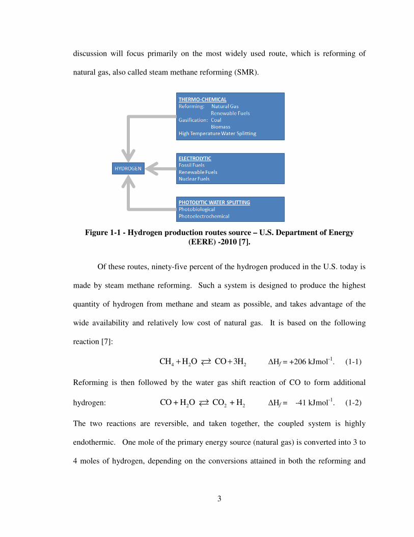
Hydrogen can be produced by three main types of processes: (1) thermo-
chemical, (2) electrolytic, or (3) photolytic. Figure 1-1 shows that even within these
three main categories, several primary energy sources may be used. The following
3
discussion will focus primarily on the most widely used route, which is reforming of
natural gas, also called steam methane reforming (SMR).
Figure 1-1 - Hydrogen production routes source – U.S. Department of Energy
(EERE) -2010 [7].
Of these routes, ninety-five percent of the hydrogen produced in the U.S. today is
made by steam methane reforming. Such a system is designed to produce the highest
quantity of hydrogen from methane and steam as possible, and takes advantage of the
wide availability and relatively low cost of natural gas. It is based on the following
reaction [7]:
4 2 2CH H O CO 3H+ +�
∆Hf = +206 kJmol
-1. (1-1)
Reforming is then followed by the water gas shift reaction of CO to form additional
hydrogen: 2 2 2CO + H O CO + H� ∆Hf = -41 kJmol
-1. (1-2)
The two reactions are reversible, and taken together, the coupled system is highly
endothermic. One mole of the primary energy source (natural gas) is converted into 3 to
4 moles of hydrogen, depending on the conversions attained in both the reforming and
4
the water gas shift reactions. The systems are typically operated at equilibrium which
demands temperatures and pressures greater than 800ºC, and up to 30 atm [8].
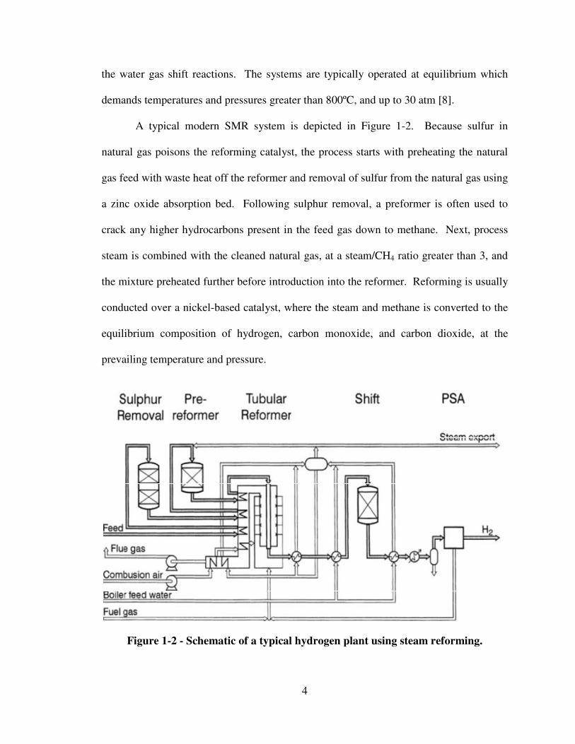
A typical modern SMR system is depicted in Figure 1-2. Because sulfur in
natural gas poisons the reforming catalyst, the process starts with preheating the natural
gas feed with waste heat off the reformer and removal of sulfur from the natural gas using
a zinc oxide absorption bed. Following sulphur removal, a preformer is often used to
crack any higher hydrocarbons present in the feed gas down to methane. Next, process
steam is combined with the cleaned natural gas, at a steam/CH4 ratio greater than 3, and
the mixture preheated further before introduction into the reformer. Reforming is usually
conducted over a nickel-based catalyst, where the steam and methane is converted to the
equilibrium composition of hydrogen, carbon monoxide, and carbon dioxide, at the
prevailing temperature and pressure.
Figure 1-2 - Schematic of a typical hydrogen plant using steam reforming.

5
The hot gas exits the reformer, and it is cooled to both generate steam for export,
and lower its temperature for the water-gas shift reactor. In the shift reactor, another
mole of hydrogen is produced from the reaction between carbon monoxide and steam to
form hydrogen and carbon dioxide. The exit of the shift reactor is further cooled for
energy recovery before feeding to a Pressure Swing Adsorption (PSA) unit to purify the
hydrogen. The purified hydrogen is sent to storage, while the rejected gas from the PSA
unit can be recycled and used as fuel, generating heat for the reformer.
The reforming reaction is highly endothermic, and requires additional energy in
the form of additional natural gas over the stoichiometric amount needed for reforming.
Discounting any export of steam, the energy efficiency is nominally 94% of theoretical,
corresponding to a net energy requirement of 320 Btu/scf of hydrogen [9].
1.2 Hydrogen markets
Hydrogen is presently used as a raw material in a broad variety of industries, from
ammonia production to glass manufacture. Except for a few limited trial applications,
hydrogen is not yet widely used as an energy carrier for transportation applications.
1.2.1 Present industrial production and usage - Compared to other commodity
bulk chemicals, hydrogen ranks second in U.S. annual production tonnage behind only
sulfuric acid (Figure 1-3). Its use benefits society in two major market areas, and several
smaller areas. By far, the worldwide use of hydrogen for production of ammonia in
agricultural fertilizers (61%), and for refining and upgrading of petroleum feed stocks
(23%) dominate the present day uses of hydrogen (Table 1-1).
Yet, while the volume of hydrogen used is large, the supply and use infrastructure
is fairly limited, because the significant production facilities are largely concentrated

6
Figure 1-3 – 2009 US annual production of key basic chemicals (million annual
metric tons) [Note 1 – US Census Bureau (2009)] [10]
[Note 2 – Pacific Northwest National Laboratory (2009)] [11].
Table 1-1 – 2003 United States and world hydrogen consumptions by end-use [12]
United States World Total
End Use Million
metric tons
Share (%) Million
metric tons
Share (%)
Ammonia 2.59 33.5 23.63 57.5
Oil Refining 3.19 41.3 11.26 27.4
Methanol 0.39 5.0 3.99 9.7
Other Uses 0.35 4.5 0.47 1.1
Merchant Sales 1.21 15.7 1.75 4.3
Total 7.73 100.00 41.09 100.00
among large internal producers and users. In the U.S., in-house captive users account for
85% of the hydrogen used, leaving 15% for outside, or merchant sales, as seen in Figure
1-4. Two reasons account for this: first, the relative inefficiency of current production
technologies drives manufacturers to build large facilities to realize economies of scale,

7
and second, the relative high cost to transport hydrogen leads to centralization of large
users close to manufacturers. Hydrogen does not have an existing large-scale distribution
Figure 1-4 – 2011 US split of hydrogen production among markets [11].
network similar to, for example, natural gas or liquid petroleum, making it expensive to
transport hydrogen over large distances. Table 1-2 shows how limited the hydrogen
pipeline distribution network is compared to the petrochemical or natural gas industries.
Several factors have limited the extensive development of a hydrogen pipeline network.
First, new construction of hydrogen pipelines are significantly more expensive than
comparable natural gas pipelines because hydrogen requires steel or alloy piping which
can resist hydrogen embrittlement. Second, former natural gas pipelines cannot easily be
converted to hydrogen service for the same reason of hydrogen embrittlement.
Additionally, pipeline fittings which are tight enough for natural gas service will not
adequately prevent hydrogen leaks from occurring at joints [13]. Other options than
Table 1-2 – Miles of U.S. gathering, transmission, and distribution pipelines [14-15]
Piping type Hydrogen[14]
Petrochemicals[15]
Natural gas[15]
Gathering and
Transmission 1,200 160,868
298,133
Distribution 1,848,980
Total 1,200 160,868 2,247,113
8
pipelines for hydrogen distribution include over the road shipments of compressed gas in
tube trailers, or liquid hydrogen in cryogenic trucks or railcars, but they are significantly
more expensive than a dedicated hydrogen pipeline system. However, depending on the
market demand for hydrogen, these alternate supply options can deliver interim volumes
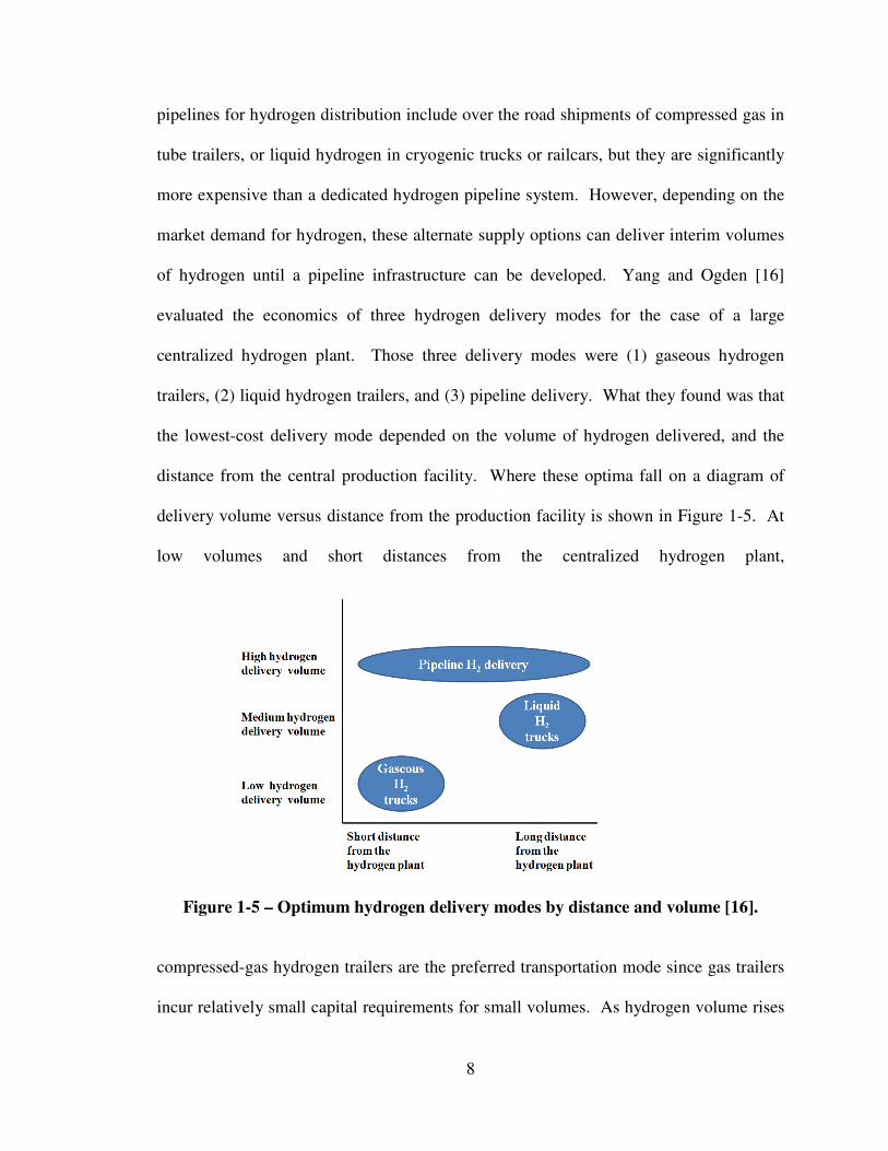
of hydrogen until a pipeline infrastructure can be developed. Yang and Ogden [16]
evaluated the economics of three hydrogen delivery modes for the case of a large
centralized hydrogen plant. Those three delivery modes were (1) gaseous hydrogen
trailers, (2) liquid hydrogen trailers, and (3) pipeline delivery. What they found was that
the lowest-cost delivery mode depended on the volume of hydrogen delivered, and the
distance from the central production facility. Where these optima fall on a diagram of
delivery volume versus distance from the production facility is shown in Figure 1-5. At
low volumes and short distances from the centralized hydrogen plant,
Figure 1-5 – Optimum hydrogen delivery modes by distance and volume [16].
compressed-gas hydrogen trailers are the preferred transportation mode since gas trailers
incur relatively small capital requirements for small volumes. As hydrogen volume rises
9
to medium, and delivery distances become long, then liquefied hydrogen trucks become
the preferred delivery option. The savings from higher load density of liquid versus gas
are partially offset by the capital and electricity requirements for liquefaction. The
liquefaction costs overshadow the fuel costs for longer transportation, so longer distances
are still economical. At large delivery volumes for either close or distant users, pipeline
delivery is always the preferred mode.
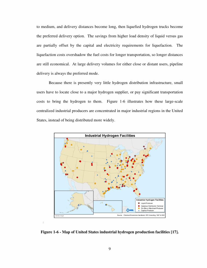
Because there is presently very little hydrogen distribution infrastructure, small
users have to locate close to a major hydrogen supplier, or pay significant transportation
costs to bring the hydrogen to them. Figure 1-6 illustrates how these large-scale
centralized industrial producers are concentrated in major industrial regions in the United
States, instead of being distributed more widely.
Figure 1-6 - Map of United States industrial hydrogen production facilities [17].

10
1.2.2 Transportation fuel - A more detailed look at the major hydrogen end-uses
in 2003 in the United States in Table 1-3 highlights two facts: (1) Bulk chemical users in
refining, fertilizer (ammonia), and methanol dominated the hydrogen usage with almost
98.7% of the demand, and (2) transportation and stationary energy demands for hydrogen
were so undeveloped that they were not even mentioned in the 2003 data. The rest of the
hydrogen not consumed by the big 3 users above was taken by the small merchant users,
with just over 1.3% of U.S. hydrogen demand in 2003.
Table 1-3 – 2003 United States annual hydrogen consumptions by end-use [12]
End Use kilotons Share (%) Small Users Total(%)
Refining 4,084 56.82
Ammonia Mfg. 2,616 36.39
Methanol Mfg. 393 5.47
Metal Mfg. 47.8 0.66
Edible fats and oils 22.1 0.31 1.32
Electronics 13.7 0.19
Aerospace, float glass 11.3 0.16
Total 7,187.9 100.000
Future transportation energy challenges lie ahead as significant social and
economic factors drive the development and future growth of hydrogen usage in the
transportation sector. These factors include: (1) national security as political instabilities
impact the availability of current oil imports, (2) global climate change and degradation
of the environment from greenhouse gas emissions from current energy sources, (3)
population and economic growth expanding the overall energy demand, (4) need for new
and clean energy at affordable prices, and (5) need to improve air quality and reduce
vehicle emissions [18].
11
In 2010, the number of registered highway vehicles in the United States numbered
over 250 million [19], practically all of them fueled with petroleum-based energy. If, in
25 years, 100 million were replaced with fuel-cell powered vehicles utilizing hydrogen, it
would require an annual hydrogen production capacity of 40,000 kilotons/year [18]. In
comparison, the 2003 industrial hydrogen consumption in the United States totaled only
7,200 annual kilotons (Table 1-3). To supply one hundred million hydrogen fuel cell
vehicles in 25 years requires more than a 5-fold increase in production of hydrogen over
2003, not including industrial uses.
Clearly, the goal of a hydrogen-fueled transportation future is very ambitious if it
is going to require a several-fold increase in the production of hydrogen over today’s
production. Adding to the difficulty is the lack of a distribution network, as evidenced by
the relatively few miles of hydrogen distribution piping as shown in Table 1-2. Thus,
while the potential future market for hydrogen as a transportation fuel is extremely large,
it will require several intermediate stages of development to reach the ultimate goal of a
hydrogen-fueled economy. The U.S. Department of Energy recognizes the level of
difficulty to reach this goal, and acknowledges that intermediate stages, such as starting
out with a distributed hydrogen system consisting of numerous small localized hydrogen
generating systems, could lead the way towards a hydrogen-fueled economy.
Demonstrating how a competitive, small-scale localized hydrogen generating plant could
be designed and built for a distributed hydrogen production scenario is the main objective
of this dissertation.
1.2.3 Stationary power - A current growth area for hydrogen demand is
stationary fuel-cell power plants [20]. Benefits of hydrogen powered fuel-cell stationary

12
power systems include (1) less noise than comparable diesel internal combustion power
systems, (2) less air pollution than diesel, gasoline, or propane engines, and (3) higher
reliability. In 2008, the total amount of commercial fuel-cell energy totaled over 13,000
kW [20]. Table 1-4 provides details on how this energy was spread out amongst primary,
auxiliary, and backup power. The installed kW is but a small fraction of the total 170
billion kW of installed back-up power capacity in the U.S [21], and it indicates how large
the potential market is for hydrogen-fueled stationary power systems.
Table 1-4 – Stationary power systems installed in the U.S. by December 2008 [20]
Total kW capacity of fuel cells operational in 2008 13,092 kW
Production capacity of fuel cells for:
Primary power 300 kW
Auxiliary power 2,761 kW
Back-up power 10,072 kW
Total kW of installed backup power, of all types 170,000,000 kW
1.2.4 Other uses – As was seen in Table 1-3, there presently exists numerous
smaller, non-energy-related uses for hydrogen in areas as diverse as float glass
manufacture, hydrogenation of edible fats and oils, and steel manufacture. A new
application, under development since 2000 by the American Iron and Steel Institute and
the University of Utah, is the utilization of hydrogen as a combination reducing agent and
fuel in the production of steel to reduce greenhouse emissions of carbon dioxide [22]. If
successful, this technology will reduce carbon dioxide emissions per ton of hot metal
during steelmaking from 1,671 kg. to 71 kg. CO2. The hydrogen demand that will be
created by this technology is 83 kg. H2 per ton of hot metal produced [23].

13
1.3 Supply strategies to develop hydrogen as a transportation fuel
To progress toward the long term vision of a hydrogen-energy powered economy,
three key factors must be in place (1) consumer acceptance of hydrogen as a replacement
for petroleum-based energy without sacrificing vehicle range, economy, or safety, (2)
reliable, affordable hydrogen-powered vehicles from major manufacturers, and (3)
convenient and affordable hydrogen supply infrastructure. These three factors are all
interrelated, in that consumers would be reluctant to purchase hydrogen-powered vehicles
if vehicle manufacturers did not provide reliable, affordable options. By the same token,
vehicle manufacturers are reluctant to undertake large-scale development of hydrogen-
powered vehicles without development of the refueling infrastructure needed to support
wide-spread adoption of hydrogen-powered transportation.
There are four major options to develop the fuel supply infrastructure needed to
progress toward a hydrogen economy: (1) develop and implement mobile reforming
technology to generate hydrogen from gasoline, compressed natural gas, ethanol, or
methanol aboard the vehicle itself, and thus take advantage of existing distribution
channels for these fuels, (2) produce hydrogen in large, centralized plants, with transport
via pipeline or tank trucks / railcars to distributed fueling stations as needed, (3) produce
hydrogen via reforming of gasoline, natural gas, ethanol, or methanol on-site in small
units at distributed decentralized locations based on local demand, and (4) phase-wise
development of hydrogen supply using option three, followed by option two. Phase one
would consist of distributed systems based on small local reforming systems in order to
build market acceptance without committing to the large capital needed for large
centralized reforming plants for transportation needs. When market acceptance has been

14
achieved through phase one, then phase two, large scale centralized hydrogen
manufacture, supported by an updated distribution network, would be able to realize
economies of scale and lower the cost of hydrogen. According to the U.S. Department of
Energy, “Distributed production is the most viable option for introducing hydrogen and
building hydrogen infrastructure,” [24].
1.3.1 Mobile on-board hydrogen generation - This option lets users re-fuel their
vehicles with currently-available gasoline, natural gas, ethanol, or methanol. Existing
distribution channels for these fuels either already exist, or can be augmented relatively
easily, which addresses the distribution infrastructure issue. Hydrogen for the vehicle’s
fuel cell is generated from a mobile on-board reforming system that runs on demand to
partially oxidize the hydrocarbon fuel according to this generic equation [25];
CnHmOp + x O2 + (2n-2x-p) H2O � n CO2 + (2n-2x-p+m/2) H2. (1-3)
Control of the oxygen to fuel ratio for Equation (1-3) at low levels of x is critical to avoid
total oxidation of the hydrocarbon fuel to CO2 and H2O by this reaction;
CnHmOp + (n+m/4-p/2) O2 � n CO2 + m/2 H2O, (1-4)
which produces no hydrogen. While conventional fuels for such systems are readily
available, the added complexity and weight exact a penalty in higher purchase price,
extra maintenance cost, and lower fuel economy, all factors which work against it from a
user perspective. If these negative factors alone weren’t enough to discourage wide-
spread adoption of this option, the U.S. Department of Energy assessed the likelihood of
this technology’s successful commercial implementation by 2015, and found enough
gaps in the development of the technology, that it recommended dropping government
R&D support in 2004 [26]. However, this route is still being pursued by a limited
15
number of developers for niche markets, such as for U.S. military applications, where
performance needs take priority over other factors, like maintenance cost or initial
investment [27].
1.3.2 Centralized hydrogen production - Due to economies of scale, hydrogen
can be produced at reasonable and competitive prices when large centralized
manufacturing facilities are used. However, the lack of an established distribution system
remains a significant hurdle to near-term implementation. The U.S. Department of
Energy envisions three primary distribution options which could be implemented to
support large centralized hydrogen manufacturing facilities [28].
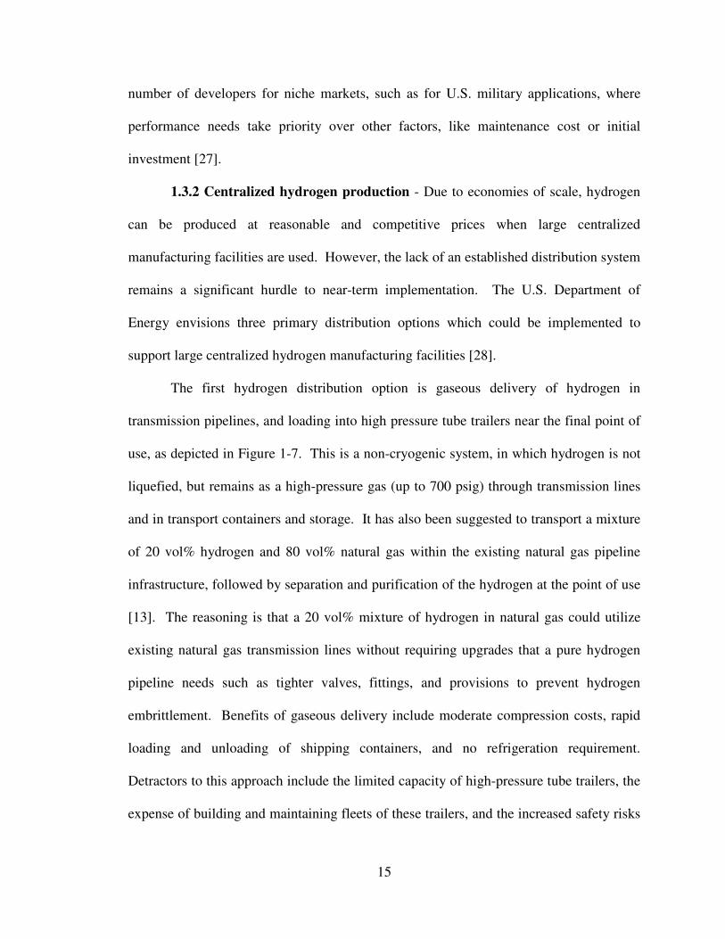
The first hydrogen distribution option is gaseous delivery of hydrogen in
transmission pipelines, and loading into high pressure tube trailers near the final point of
use, as depicted in Figure 1-7. This is a non-cryogenic system, in which hydrogen is not
liquefied, but remains as a high-pressure gas (up to 700 psig) through transmission lines
and in transport containers and storage. It has also been suggested to transport a mixture
of 20 vol% hydrogen and 80 vol% natural gas within the existing natural gas pipeline
infrastructure, followed by separation and purification of the hydrogen at the point of use
[13]. The reasoning is that a 20 vol% mixture of hydrogen in natural gas could utilize
existing natural gas transmission lines without requiring upgrades that a pure hydrogen
pipeline needs such as tighter valves, fittings, and provisions to prevent hydrogen
embrittlement. Benefits of gaseous delivery include moderate compression costs, rapid
loading and unloading of shipping containers, and no refrigeration requirement.
Detractors to this approach include the limited capacity of high-pressure tube trailers, the
expense of building and maintaining fleets of these trailers, and the increased safety risks
16
of handling, transporting, and offloading bulk quantities of flammable materials under
high pressure within residential communities. The U.S. Department of Energy convened
a national workshop in 2003 to review all modes of hydrogen distribution and delivery,
including gas delivery pipelines [29]. One outcome of this conference was identification
of the key R&D needs for large-scale installation of hydrogen gas delivery pipelines.
Open issues which were discussed included lack of affordable, effective leak-detection
equipment, incomplete understanding of material science with regards to hydrogen
embrittlement and fatigue cracking, and insufficient industry operating experience,
including incomplete safety assurance procedures and standards. Nevertheless, delivery
by gas pipeline is the lowest cost delivery option at high volumes, and as the
development issues are sorted out, is likely to remain a significant part in the future
hydrogen delivery infrastructure.
Figure 1-7 – Gaseous hydrogen delivery pathway [28].
17
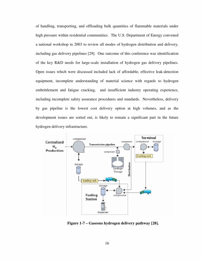
The second hydrogen distribution option is cryogenic liquid hydrogen delivery via
liquid hydrogen tank trailers, as depicted in Figure 1-8. With cryogenic delivery,
significantly more hydrogen per truckload is possible, so the efficiency of delivery is
enhanced. It comes, however, at a price due to higher expenses for compression,
liquefaction, and refrigeration. The U.S. Department of Energy’s “strategic directions for
hydrogen delivery” workshop [29] identified key issues regarding liquid hydrogen
delivery, including cryogenic liquid boil-off management, high cost of materials of
construction for cryogenic systems, public safety in case of leaks (leak detection,
odorization, and lack of a visible flame), and inconsistency of codes and standards
between federal, state and local agencies. Even with these development gaps, the U.S.
Department of Energy envisions that liquid hydrogen delivery will most likely play a role
in at least the initial phases of the of the buildup of the hydrogen delivery infrastructure
because of its higher delivery density over non-cryogenic compressed-gas trailers.
Figure 1-8 – Cryogenic liquid hydrogen delivery [28].

18
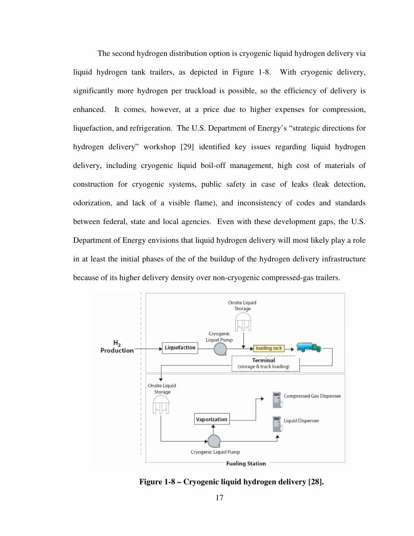
The third hydrogen distribution option is high energy density liquid or solid
hydrogen carriers that are transported relatively economically, then treated at their point
of use to release the hydrogen. One variant of this option is to transport conventional
primary energy sources such as natural gas, ethanol, methanol, or liquids produced from
biomass to local fuel stations and reform them into hydrogen. However, conventional
primary energy carriers of this type do not fit the concept of centralized production of
hydrogen, and are more properly called feedstocks for a distributed hydrogen production
scenario, discussed in section 1.3.3 below. More germane to a centralized-production
carrier-based distribution system are novel carriers such as chemical or metal hydrides, or
other hydrogen-containing solids or liquids that are treated to release hydrogen at a
refueling station or other point of use, which might even be on-board a vehicle, as shown
in Figure 1-9. The goals of these novel hydrogen carriers are to (1) have an adequately
high hydrogen carrying capacity per transport trailer to be economical, and (2) have the
durability to withstand over a thousand load/unload cycles without appreciable loss of
capacity [28].
One example of a novel liquid hydrogen carrier is the dehydrogenation of liquid
methylcyclohexane with a catalyst aboard a vehicle to produce toluene and three
hydrogen molecules per reaction 1-3 [30]:
C6H11CH3 Catalyst
→ C6H5CH3 + 3 H2. (1-5)
The spent toluene is returned to a chemical plant where hydrogen is added back to
produce methylcyclohexane, and the cycle is repeated. In this method, the hydrogen is
6% of the weight of the methylcyclohexane, which has a density of 0.77 g/cm3.
Therefore, the volumetric hydrogen density of this carrier is approximately 0.046 g/cm3,
19
Figure 1-9 – Alternative carrier hydrogen delivery [28].
or 46 g/liter. This option exceeds the U.S. Department of Energy’s hydrogen interim
2015 hydrogen density goals of 5.5 wt% and 40 g/liter, as shown in Figure 1-10, but is
still short of the ultimate targets of 7.5% wt% and 70 g/liter. The other novel carriers
under consideration in Figure 1-10 are all generally inferior to liquid hydrogen. The only
exceptions are the ultra-high pressure options (cryogenically-compressed to 350 bar, and
700 bar). However, even these ultra-high pressure options do not achieve the 2015
density targets, much less the ultimate targets. Additionally, the cost per kWh of these
options are still significantly higher than the 2015 target of 2 $USD/kWh, as seen in
Figure 1-11 [32]. Clearly, these novel carriers are not yet technically or economically
able to provide a distribution system for a centralized hydrogen production scenario,
without significant further improvements.
20
Figure 1-10 – Capacities of hydrogen carriers [31].
Figure 1-11 – $/kWh of hydrogen carriers as of 2007 [32].
1.3.3 Distributed hydrogen production - Localized hydrogen production located
nearer the points of use using numerous on-site small-scale manufacturing units is termed
the “distributed supply” pathway to the hydrogen economy. This system provides the
transitional hydrogen supply infrastructure with enough convenience and an adequate
number of consumer hydrogen outlets to foster faster acceptance of hydrogen-powered
hybrid fuel-cell vehicles. Spreading out hydrogen production over multiple small units

21
near users saves the cost of transportation and pipeline networks compared to large
centralized hydrogen plants. Using steam methane reforming for the small on-site
production plants takes advantage of the extensive pre-existing natural gas distribution
network to supply them through many regions of the country. A drawback of this scheme
versus large centralized production of hydrogen, however, is that carbon sequestration of
carbon dioxide left over after steam methane reforming is uneconomical for small
reforming units. Therefore, this scheme does not help the greenhouse gas emission issue
associated with hydrogen produced from steam methane reforming. Carbon-free
hydrogen production in small distributed localized hydrolysis units may solve the
greenhouse gas emissions issue for a distributed hydrogen supply scenario, but
electrolysis in general is uneconomical compared to steam methane reforming at all
scales, in both capital cost and energy efficiency. Figure 1-12 compares the well to
wheels costs and carbon footprints from several fuel pathways, and shows the cost and
environmental advantages of hydrogen from natural gas versus electrolysis [33].
Figure 1-12 – Comparison of fuel pathways regarding emissions and costs [33].

22
1.3.4 Phase-wise distributed to centralized evolution - As stated previously,
a major hurdle hindering the progress toward the ultimate goal of a widespread hydrogen-
fueled economy is lack of a distribution system for large centralized hydrogen plants,
which are the most economical means of hydrogen production on a large scale.
Producers are reluctant to commit to the large investment required for large centralized
hydrogen production plants if there are no means for delivering the hydrogen to users.
Likewise, users have no incentive to switch to hydrogen fuel if it is not as readily
available as traditional fuels.
A future hydrogen-fueled U.S. economy in which hydrogen-fueled vehicles
become commonplace requires considerably more hydrogen than is produced today.
The U.S. Department of energy estimates, that for every 100 million vehicles on the road,
approximately 40 million annual tons of hydrogen supply are required [18]. The two
main supply strategies for providing this hydrogen are centralized production (section
1.3.2) or distributed production (section 1.3.3). If the supply were met by only
centralized supply, or only by distributed supply, the number of equivalent plants
required to produce 40 million tons of hydrogen (per 100 million vehicles) for each of
these options would be one of the choices as spelled out in Table 1-5.
Table 1-5 – Other options to produce 40 million annual tons of hydrogen [18]
Centralized production options to produce 40 million tons of hydrogen
Coal/biomass gasification (SMR) 140 plants Similar to today’s large
coal-fired plants
Nuclear water splitting 100 plants Nuclear plants making only
hydrogen
Oil and natural gas refinery (SMR) 20 plants Each the size of a small oil
refinery
Distributed production options to produce 40 million tons of hydrogen
Electrolysis 1,000,000 plants Small, neighborhood-based
units
Small on-site reformers (SMR) 67,000 plants About 1/3 the present
number of gas stations
23
It would be risky to settle on just one option in Table 1-5. Doing so carries the
risk that it might be the wrong choice over the long term, which might not be evident
until extensive investment had been needlessly expended. Therefore, a less risky
approach is to implement multiple options of technology from Table 1-5, in a phased
progression. Two reasons make this phase-wise approach using multiple options less
risky than the single-option approach: (1) multiple technology options can be developed
in parallel, lessening the technical and economic risk, and (2) today’s lack of a hydrogen
distribution infrastructure can be addressed, at least temporarily, by starting off with a
distributed supply strategy, followed by a gradual shift toward a more centralized supply
system as the market develops and the centralized supply system infrastructure is built.
The U.S. Department of Energy recognizes that a transitional phase-wise strategy
is needed as a means to jumpstart and develop the consumption side of the hydrogen fuel
market before a large scale hydrogen distribution network can be built [18]. Initially, on-
site production via distributed manufacturing facilities will gradually build a user base.
The distributed manufacturing phase will take advantage of existing energy distribution
networks like natural gas, so availability of hydrogen can be widespread and convenient,
to encourage manufacturers to build vehicles, and users to begin switching to hydrogen as
a transportation fuel. While this market is being established, infrastructure for large
scale hydrogen distribution based on large centralized production facilities could be built.
One possible scenario for supply might evolve as shown in Table 1-6, with a variety of
technologies co-existing as the market shakes out.
The U.S. Department of Energy expects that this phase-wise development could
take decades to occur, and involve further evolution and breakthroughs in all facets of the
24
Table 1-6 – Parallel multi-technology options to produce 40 million annual tons of
hydrogen [18]
Technology Number of
plants
Annual H2
production
Equivalent
automobiles
Early market development phase (focused on distributed manufacturing)
Neighborhood
electrolyzers 100,000 4 million tons 11.1 million
Small reformers in
refueling stations 15,000 8 million tons 22.2 million
Mature phase (focused on centralized manufacturing)
Coal/biomass gasification
plants 30 8 million tons 22.2 million
Nuclear water splitting
plants 10 4 million tons 11.1 million
Large oil and gas
SMR/gasification
refineries
7 16 million tons 44.4 million
Totals 40 million tons 111 million
hydrogen economy, from generation, distribution, and consumption of hydrogen, as seen
in a possible scenario depicted in Figure 1-13 [6]. It graphically shows how a distributed
production strategy early on eventually gives way to centralized production as the
hydrogen economy develops.
Figure 1-13 – Possible evolution of hydrogen technologies [6].
25
1.4 Incentives for current research
As shown in Figure 1-13 above, a key feature in the early stages of the journey
towards a hydrogen economy is to pursue a distributed supply strategy by developing
small scale on-site steam methane reforming hydrogen production units. Since 1 kg of
hydrogen has approximately the same energy content as a gallon of gasoline, the U.S.
Department of energy has used the price of gasoline as a basis of comparison for the
target hydrogen production price. This gives consumers an easily-comprehended scale of
comparison when evaluating the cost of conventionally-fueled versus hydrogen-fueled
transportation. The U.S. Department of Energy initially proposed a hydrogen cost target
of $2 to $3 per kg of hydrogen to induce consumers to begin switching from traditional
fuels over to hydrogen. Since then, however, as gasoline prices have escalated faster than
initial projections, this target may have to be revised upward. Developing small-scale
reformers to meet this challenge by improving efficiency and reducing the cost of the
technology is the focus of current research in this area at the University of Houston.
26
CHAPTER TWO
Background – steam methane reforming, heat pipes, ceramic foam reactors, and
catalytic combustion
2.1 Introduction
This chapter begins with a review of process and operating details for
conventional steam methane reforming systems, and the implications of scaling down this
technology to the size needed for small on-site distributed hydrogen generating plants.
Next, several technological advancements applicable to steam methane reforming,
namely, heat pipes, ceramic foam catalyst substrates, and catalytic combustion are
discussed. Finally, the results of prior research conducted at the University of Houston
on utilizing these technological advancements to improve the cost and efficiency of
small-scale steam methane reforming systems are reviewed. From the results of these
discussions and reviews, the goals of this dissertation research are presented.
2.2 Steam methane reforming
Steam methane reforming is the dominant technology for hydrogen production in
the U.S., accounting for 95% of production [7]. Such a system is designed to produce the
highest quantity of hydrogen from the methane and steam feeds as possible.
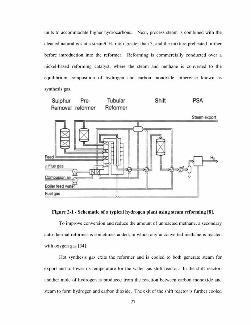
A typical modern SMR system is depicted in Figure 2-1. Because sulfur in
natural gas poisons the reforming catalyst, the process starts with preheating of the
natural gas feed from waste heat off the reformer and removal of sulfur from the natural
gas using a zinc oxide guard bed. Following sulphur removal, a preformer is often used
to crack any higher hydrocarbons present in the feed gas down to methane, CH4. Pre-
forming of higher hydrocarbons down to methane allows the downstream reformer to be
optimally designed and built smaller to handle just methane, instead of requiring larger
27
units to accommodate higher hydrocarbons. Next, process steam is combined with the
cleaned natural gas at a steam/CH4 ratio greater than 3, and the mixture preheated further
before introduction into the reformer. Reforming is commercially conducted over a
nickel-based reforming catalyst, where the steam and methane is converted to the
equilibrium composition of hydrogen and carbon monoxide, otherwise known as
synthesis gas.
Figure 2-1 - Schematic of a typical hydrogen plant using steam reforming [8].
To improve conversion and reduce the amount of unreacted methane, a secondary
auto-thermal reformer is sometimes added, in which any unconverted methane is reacted
with oxygen gas [34].
Hot synthesis gas exits the reformer and is cooled to both generate steam for
export and to lower its temperature for the water-gas shift reactor. In the shift reactor,
another mole of hydrogen is produced from the reaction between carbon monoxide and
steam to form hydrogen and carbon dioxide. The exit of the shift reactor is further cooled
28
for energy recovery before feeding the Pressure Swing Adsorption (PSA) unit to purify
the hydrogen. The purified hydrogen is sent to storage, while the rejected gas from the
PSA unit is recycled and used as part of the fuel for the reformer.
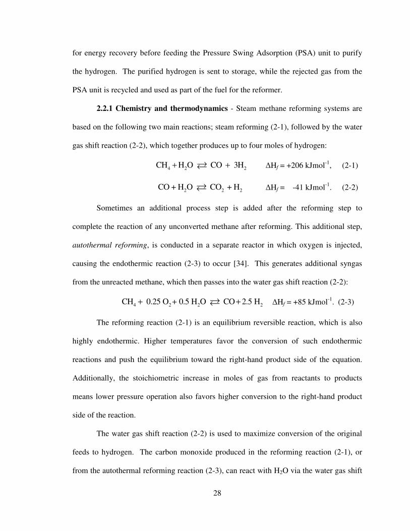
2.2.1 Chemistry and thermodynamics - Steam methane reforming systems are
based on the following two main reactions; steam reforming (2-1), followed by the water
gas shift reaction (2-2), which together produces up to four moles of hydrogen:
4 2 2CH H O CO 3H+ +�
∆Hf = +206 kJmol
-1, (2-1)
2 2 2CO + H O CO + H� ∆Hf = -41 kJmol
-1. (2-2)
Sometimes an additional process step is added after the reforming step to
complete the reaction of any unconverted methane after reforming. This additional step,
autothermal reforming, is conducted in a separate reactor in which oxygen is injected,
causing the endothermic reaction (2-3) to occur [34]. This generates additional syngas
from the unreacted methane, which then passes into the water gas shift reaction (2-2):
4 2 2 2CH 0.25 O + 0.5 H O CO 2.5 H+ +�
∆Hf = +85 kJmol
-1. (2-3)
The reforming reaction (2-1) is an equilibrium reversible reaction, which is also
highly endothermic. Higher temperatures favor the conversion of such endothermic
reactions and push the equilibrium toward the right-hand product side of the equation.
Additionally, the stoichiometric increase in moles of gas from reactants to products
means lower pressure operation also favors higher conversion to the right-hand product
side of the reaction.
The water gas shift reaction (2-2) is used to maximize conversion of the original
feeds to hydrogen. The carbon monoxide produced in the reforming reaction (2-1), or
from the autothermal reforming reaction (2-3), can react with H2O via the water gas shift

29
reaction (2-2) to yield up to one additional mole of hydrogen. Like reforming, the water
gas shift reaction is also an equilibrium reaction. However, it is slightly exothermic, so
equilibrium to a higher conversion toward the right-hand product side of the reaction is
favored at lower temperatures. This reaction is unaffected by changes in pressure
because of its equimolar feed/product stoichiometry.
In summary, the main features of the reforming (2-1) and the water gas shift
reaction (2-2) are summarized in Table 2-1. We see that the equilibrium conversions of
the two reactions are impacted in opposite directions by temperature. Therefore, these
reactions must be separated and conducted in two separate reactors at different operating
conditions.
Table 2-1 – Reforming /water gas shift reaction features
Reaction Enthalpy Stoichiometry
Impact upon equilibrium
conversion by
Temperature Pressure
(2-1)
reforming endothermic
more moles of
product than
reactants
favored by
higher
temperature
favored by
lower
pressure
(2-2)
rater gas Shift exothermic equimolar
favored by
lower
temperature
no impact
Both reforming (2-1) and the water gas shift (2-2) are reversible equilibrium
reactions at typical process conditions. Therefore the reactor product composition is
determined by thermodynamics, when there are no other physical limitations in the
system like mass or heat transfer limits. Higher temperatures and lower pressure favor
increased conversion of CH4 to H2, as shown in Table 2-1. Figure 2-2 shows the
equilibrium percentage of CH4 remaining after reaction, with the system at its final

30
equilibrium. It graphically displays the trends in which higher temperature and/or lower
pressure leads to higher conversion of the CH4.
Figure 2-2 - Equilibrium percentage of CH4 after reforming [35].
Figure 2-2 above depicts the equilibrium concentration of methane alone. If the
pressure is fixed at 20 atmospheres and the steam to methane ratio at three, then
equilibrium concentrations of all the components (methane, carbon monoxide, and
hydrogen) is a function of the reforming temperature, as in Figure 2-3 [36]. Because
reforming is an endothermic reaction, there is an expected rise in conversion (higher
equilibrium concentration of the products, hydrogen and carbon monoxide). It is also
evident that conversion is essentially complete between 850 to 900ºC, so there is no point
in operating at higher temperatures.

31
Figure 2-3 – Equilibrium conversions for steam methane reforming [36].
2.2.2 Catalysts - Steam methane reforming (reaction 2-1) is catalyzed by several
metal catalysts. For instance, cobalt, platinum, palladium, iridium, ruthenium, rhodium,
and nickel have all been cited as usable for this purpose [35]. Several of them, in
particular, rhuthenium, and rhodium, exhibit extraordinarily high catalytic activity per
unit area, as seen in Figure 2-4. Even in light of this, one of the relatively lower-activity
Figure 2-4 – Catalytic metals used for steam methane reforming [36].
metals, nickel, has become the industry-standard catalytic metal used in steam methane
reforming because its relatively low cost, wide availability, and sufficient catalytic

32
activity combine to make it the most cost-efficient choice. A typical commercial catalyst
uses between 12 to 20% wt% of nickel, applied to a refractory ceramic substrate such as
α-Al2O3. Twigg relates that 20 wt% nickel is a practical upper limit for metal loading, as
designed experiments in which the catalyst nickel contents were varied from 10 to 25
wt% showed diminishing returns once the nickel content exceeded 20 wt% [35]. Since
the reforming reaction occurs on the surface of the nickel itself, maximization of the
nickel surface area available to the reacting gases is key to obtaining effective reforming
catalysts. This is done in one of two ways: (1) precipitation of nickel as an insoluble
compound from a soluble salt, or (2) impregnation with a solubilized nickel salt that is
later calcined at 600ºC into nickel oxide. In either case, the nickel oxide is reduced to the
metal using supplied hydrogen (at approximately 500ºC) before it is ready for service.
Impregnated catalysts are recognized as being stronger in use than precipitated catalysts,
and have become the dominant type of commercial reforming catalyst [35].
The water gas shift reaction (reaction 2-2) has historically been catalyzed by iron
oxide and chromium catalysts at moderate temperatures in the range of 400ºC. Recently,
however, copper-based catalysts have been proven effective at temperatures as low as
200ºC. Modern water gas shift systems have sometimes utilized two stages, a high
temperature shift at 400ºC using iron oxide/chromium catalyst, followed by a low
temperature shift at 200ºC using copper-based catalyst [35].
2.2.3 Pretreatment - Because typical catalysts used in reformers are particularly
susceptible to sulphur poisoning, feed gases must undergo pre-treatment to remove
sulphur-based contaminants. A typical sulphur-removal system for steam methane
reforming consists of a high pressure hydrogenation hydro-desulphurization catalytic unit

33
to convert sulphur-based impurities into hydrogen sulphide, followed by a zinc oxide
adsorber unit to catch the hydrogen sulphide.
Following sulphur removal, a preformer is often used to crack any higher
hydrocarbons present in the feed gas to methane, CH4. Removing higher hydrocarbons,
and therefore feeding only methane to the reformer, greatly simplifies design and
minimizes size requirements.
2.3 Steam methane reforming reaction parameters
Through decades of experience, the most important factors for insuring high yield
and long catalyst life are as follows:
2.3.1 Reactant concentration: steam to methane ratio - Stoichiometrically, the
minimum ratio of steam to methane for the reforming reaction (2-1) and water gas shift
reaction (2-2) to proceed, is two to one (one mole of steam for each of the two reactions).
However, experience has shown that operation at stoichiometric steam to methane ratios
close to two to one lead to carbon coking on the catalyst and deactivation. On the other
hand, operation with an excess of steam inhibits coking. Therefore, steam to methane
ratios greater than two are desired. The coking reactions will be discussed in more detail
in section 2.2.6.1 below. If carried too far, however, too high a steam to methane ratio
results in excessive energy losses, and quickly becomes uneconomical. Typical
commercially-viable steam to methane ratios range from 2.5:1 to 3.5:1 [35].
2.3.2 Reformer temperature - Within the reformer, methane thermally crack s
into elemental carbon and hydrogen at elevated temperatures, as shown in reaction 2-4:
4 2CH C 2H+� . ∆Hf = +74.9 kJmol
-1. (2-4)
34
The carbon formed fouls catalyst pores and leads to deactivation. Since this cracking
reaction is endothermic, the equilibrium toward the right to form additional carbon is
favored as the temperature is increased in the reformer. The greatest risk of carbon
formation is near the inlet, where the CH4 concentration is the highest. Experience has
shown that a normal inlet temperature of 450 to 550ºC keeps carbon formation to a
minimum.
As for the main section of the reformer past the inlet, the reforming reaction (2-1)
is endothermic. Therefore, conversions of CH4 and yields of H2 are higher when the
reformer is at as high a temperature as can be achieved. Figure 2-3, however, showed
that the equilibrium conversion levels off at approximately 800 to 900ºC, so there is no
incentive to go higher. Thus, 800 to 850ºC is a typical operating temperature for current
commercial steam methane reformers.
2.3.3 Pressure - Low pressure favors conversion for the reforming reaction (2-1)
since the stoichiometry yields more moles of gaseous product on the right hand side of
the reaction equation. However, operating at lower pressure to improve equilibrium H2
yields has diminishing returns, since lower pressure operation increases the size and cost
of gas handling equipment, including piping, compressors, and gas-phase heat
exchangers. These types of equipment are smaller, of higher efficiency, and of lesser
cost when operating at higher pressures. Pressure drop through the system must also be
taken into account, which means that inlet pressures are usually at a minimum of 5 atm or
more. However, it is not unusual to operate a steam methane reformer at 20 atmospheres
of pressure, for example, in ammonia or methanol reforming plants where further
compression to higher pressures are required.
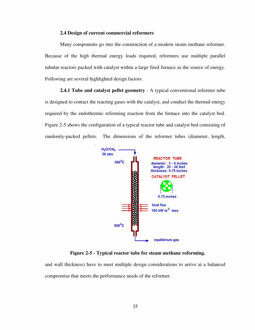
35
2.4 Design of current commercial reformers
Many components go into the construction of a modern steam methane reformer.
Because of the high thermal energy loads required, reformers use multiple parallel
tubular reactors packed with catalyst within a large fired furnace as the source of energy.
Following are several highlighted design factors.
2.4.1 Tube and catalyst pellet geometry - A typical conventional reformer tube
is designed to contact the reacting gases with the catalyst, and conduct the thermal energy
required by the endothermic reforming reaction from the furnace into the catalyst bed.
Figure 2-5 shows the configuration of a typical reactor tube and catalyst bed consisting of
randomly-packed pellets. The dimensions of the reformer tubes (diameter, length,
Figure 2-5 - Typical reactor tube for steam methane reforming.
and wall thickness) have to meet multiple design considerations to arrive at a balanced
compromise that meets the performance needs of the reformer.

36
(a) Tube diameter – The steam reforming reaction is so endothermic that heat transfer
into the reactor will limit the reaction unless the reactor has a sufficient surface to volume
ratio. Increased diameter will enable more catalyst to be loaded into a given tube with a
resulting increase of productivity. However, tubes larger than 130 mm (7 inches) in
diameter soon become limited on heat transfer into the center axis of the catalyst in the
tube, leading to a loss of reaction rates. Conversely, if the diameter is decreased to less
than 75 mm (3 inches) to ensure that the heat transfer is most effective, then pressure
drop in the smaller tubes becomes excessive. Figure 2-6 shows the relative percent
pressure drop of various sizes of a commercial reforming catalyst, and how the smaller
sizes suffer from higher relative pressure drop. Commercial reformer tubes strike a
balance between pressure drop and heat transfer with normal internal diameters ranging
Figure 2-6 - Relative Pressure drop vs. catalyst pellet size [37].
from 70 to 130 mm (2.8 to 5 inches) [35]. A tube diameter of 100 mm (4 inches) is
commonly used in most reformers today.
The geometry of the catalyst pellets is based on large rings or perforated discs in
order to prevent excessive pressure drops along the length of the bed. Their sizes are

37
kept relatively large, on the order of 1/6th
the diameter of the tube. This is so that, even if
individual pellets fracture into multiple pieces from handling, thermal expansion or
contraction, the broken pieces are still large enough to avoid plugging the tube and
creating high pressure drop. A consequence of the large pellet size is that pore diffusion
is limited, and effectiveness factors of less than 0.05 are typical. Perforated discs will
often have 4 or more perforations as shown in Figure 2-5 to provide additional surface
area for reaction.
(b) Tube length - longer tube length is usually more cost-effective than increasing the
number of tubes because of the associated cost of manifold connections, expansion joints,
etc., when additional tubes are added. However, this trend holds up only up to the point
where excessive length begins to create too high a pressure drop, or increases the risk of
structural failure when the length of the tube is too long to support its own weight. Seven
to ten meters is a nominal length for commercial reformer tubes today, striking a balance
between added catalyst loading and structural strength.
(c) Tube wall thickness - The wall thickness of a reformer tube directly affects both
construction costs and operational costs. Building a reformer with excessively thick
reformer tubes is more costly from a materials standpoint, since the materials of
construction needed to withstand the temperatures in a fired-reformer furnace of over
1000ºC are quite expensive. Additionally, the higher mass of thicker tubes limit builders
to shorter tube lengths because of strength limitations of the support structures that have
to hold these heavier tubes in place. Excessively thick tubes also require smaller catalyst
pellets that are able to fit into the smaller bores of the thick tubes. It is shown above that
smaller catalyst pellets lead to higher pressure drop and higher operating costs. Lastly,

38
thicker reformer tube walls create a higher thermal resistance at the wall, increasing the
required wall temperature on the fired side of the tube, which increases both the energy
costs, as well as shortens the tube life due to increased metal creep. The lower limit of
tube wall thickness is set by the strength requirements of the reformer design, and is
usually approximately 20 mm (0.75 inch).
(d) Temperature profile – To reduce carbon formation, the feed gas enters the reactor at
about 500ºC (Figure 2-5) and is heated to an outlet temperature of 800ºC. Since reaction
rates are highest at the inlet, where methane concentration is the highest, there is an
increase in the heat flux at the tube surface that increases along the tube from inlet to
outlet. In fact, initially the temperature at the inlet may even decrease and then recover
after passing through a minimum, giving a typical axial temperature profile shown in
Figure 2-7.
Figure 2-7 - Typical steam methane reformer tube axial temperature profile.
2.4.2 Materials of construction - Reformer reactor tubes cannot withstand
unlimited high temperatures or limited startups and shutdowns. Starting up from a cold
shutdown raises the temperature of a reactor tube from 25 to 800ºC. Thermal expansion
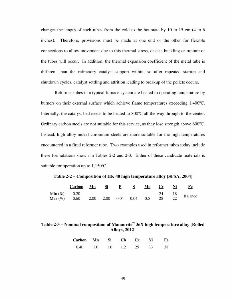
39
changes the length of such tubes from the cold to the hot state by 10 to 15 cm (4 to 6
inches). Therefore, provisions must be made at one end or the other for flexible
connections to allow movement due to this thermal stress, or else buckling or rupture of
the tubes will occur. In addition, the thermal expansion coefficient of the metal tube is
different than the refractory catalyst support within, so after repeated startup and
shutdown cycles, catalyst settling and attrition leading to breakup of the pellets occurs.
Reformer tubes in a typical furnace system are heated to operating temperature by
burners on their external surface which achieve flame temperatures exceeding 1,400ºC.
Internally, the catalyst bed needs to be heated to 800ºC all the way through to the center.
Ordinary carbon steels are not suitable for this service, as they lose strength above 600ºC.
Instead, high alloy nickel chromium steels are more suitable for the high temperatures
encountered in a fired reformer tube. Two examples used in reformer tubes today include
these formulations shown in Tables 2-2 and 2-3. Either of these candidate materials is
suitable for operation up to 1,150ºC.
Table 2-2 – Composition of HK 40 high temperature alloy [SFSA, 2004]
Carbon Mn Si P S Mo Cr Ni Fe
Min (%) 0.20 - - - - - 24 18 Balance
Max (%) 0.60 2.00 2.00 0.04 0.04 0.5 28 22
Table 2-3 – Nominal composition of Manaurite®
36X high temperature alloy [Rolled
Alloys, 2012]
Carbon Mn Si Cb Cr Ni Fe
0.40 1.0 1.0 1.2 25 33 38

40
2.4.3 Furnace configuration and burner arrangements - For fired tube reform-
ers, the arrangement of the burners which provide the thermal energy for the endothermic
reforming reaction play a large part in determining how well the system performs. There
are two design goals for an ideal furnace:
(1) Even heat flux horizontally across the banks of reformer tubes. Uneven heat flux in a
non-ideal furnace gives rise to uneven tube heating and variations in reactivity,
productivity, and life from tube to tube. When such tube to tube deviations occur, the
overall efficiency of the entire reformer furnace does not reach the maximum attainable if
all the tubes were operating with uniform reactivity and productivity.
(2) Vertical heat flux gradients tailored to the energy demand along the length of the tube.
Maximum heat flux is applied to the active reaction zone of the reformer tube, and less
heat flux applied where the reaction is not as active. Typically, most of the reforming
reaction occurs in the first half of the tube. When a reformer tube has new catalyst, the
active zone, where thermal energy is needed most, is near the inlet. As the catalyst ages,
the active reaction zone migrates downward through the bed. Therefore, the wall flux in
an ideal furnace must adjust the position of the heat flux profile up or down along the
length of the tube.
Furnaces for reformers today are of four major types, shown here in Figure 2-8,
and described below:
(a) bottom fired – This configuration is a counter-current flow arrangement with respect
to the reactants versus the burner gases, and achieves an approximately constant heat flux
profile along the length of the tube. However, a constant heat flux along the length of the
tube is not optimal, if a profiled heat flux is called for. Therefore, control of a profiled
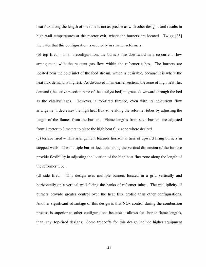
41
heat flux along the length of the tube is not as precise as with other designs, and results in
high wall temperatures at the reactor exit, where the burners are located. Twigg [35]
indicates that this configuration is used only in smaller reformers.
(b) top fired – In this configuration, the burners fire downward in a co-current flow
arrangement with the reactant gas flow within the reformer tubes. The burners are
located near the cold inlet of the feed stream, which is desirable, because it is where the
heat flux demand is highest. As discussed in an earlier section, the zone of high heat flux
demand (the active reaction zone of the catalyst bed) migrates downward through the bed
as the catalyst ages. However, a top-fired furnace, even with its co-current flow
arrangement, decreases the high heat flux zone along the reformer tubes by adjusting the
length of the flames from the burners. Flame lengths from such burners are adjusted
from 1 meter to 3 meters to place the high heat flux zone where desired.
(c) terrace fired – This arrangement features horizontal tiers of upward firing burners in
stepped walls. The multiple burner locations along the vertical dimension of the furnace
provide flexibility in adjusting the location of the high heat flux zone along the length of
the reformer tube.
(d) side fired – This design uses multiple burners located in a grid vertically and
horizontally on a vertical wall facing the banks of reformer tubes. The multiplicity of
burners provide greater control over the heat flux profile than other configurations.
Another significant advantage of this design is that NOx control during the combustion
process is superior to other configurations because it allows for shorter flame lengths,
than, say, top-fired designs. Some tradeoffs for this design include higher equipment

42
costs due to the higher complexity of the multi-burner control system and combustion gas
distribution to ensure even distribution of the heat flux.
Figure 2-8 - Typical configurations of reformer furnaces: (a) bottom fired, (b) top
fired, (c) terrace wall, (d) side fired [36].
2.5 Operating conditions
Successful operation of a steam methane reforming system requires keeping the
process within parameters which have been determined from years of operating
experience. Following are four major operating areas which enhance productivity,
reliability, and efficiency.
A typical commercial-scale reformer furnace is a large system in itself, requiring
significant capital investment, and has a large footprint. Figure 2-9 is a sketch of a
typical terrace-fired reformer furnace. A human figure (within the red circle) is shown
for scale to show the enormity of the furnace. Besides the reformer tubes and burners,
this diagram shows the complexity of feed distribution and product collection systems.
In the top of the furnace are shown the multiple heat exchangers which are needed to
recover the combustion energy not captured in the reformer tubes. These heat exchangers
are used to either pre-heat incoming reactant streams (saving the energy cost of
preheating these streams), or to generate steam for export to other users.
43
Figure 2-9 – Typical terrace wall reformer furnace [35].
2.5.1 Prevention of carbon fouling - Carbon fouling of the reformer catalyst can
occur from any of the following three undesired side reactions: thermal cracking of
methane (2-4), disproportionation of CO (2-5), or reduction of CO (2-6).
Thermal cracking of CH4 CH4 � C + 2 H2, ∆Hf = +74.9 kJmol-1
, (2-4)
Disproportionation of CO 2 CO � C + CO2, ∆Hf = -172.5 kJmol-1
, (2-5)
Reduction of CO CO + H2 � C + H2O, ∆Hf = -131.3 kJmol-1
. (2-6)
The first side reaction, thermal cracking of methane to carbon and hydrogen (reaction 2-
4), is endothermic, and its equilibrium is favored toward higher conversion to carbon at
higher temperatures, increasing the risk of excessive carbon deposition and catalyst
deactivation. The risk is greatest near the inlet, where the methane concentration is the
44
highest. To control the thermal cracking reaction (2-4) in the inlet section of the reformer
tubes where the methane concentration is the highest, experience has shown that a range
of inlet temperatures of from 450 to 550ºC works best.
Both of the other undesired side reactions, CO disproportionation (2-5), and CO
reduction (2-6) are exothermic, and at the normal temperatures in a reformer, tend to the
left hand sides (carbon-free) of their equilibrium equations through the catalyst bed.
Together, all three undesired side reactions occur all along the length of the
reformer catalyst bed. Carbon does not accumulate near the inlet of the reformer, where
the temperatures are less than 650ºC, because the rates of the exothermic reactions (2-5)
and (2-6) which remove carbon are faster than it is formed by the endothermic reaction
(2-4). However, once the temperature passes above 650ºC in the catalyst bed, the
methane cracking reaction (2-4) accelerates in rate enough to where carbon deposits
faster than reactions (2-5) and (2-6) remove it, and carbon accumulates. Such regions of
carbon deposition lead to zones of inactivity.
2.5.2 Prevention of hot spots or hot bands - An inactive zone fouled by carbon
no longer has the endothermic reforming reaction (2-1) to absorb the heat flux from the
reformer furnace, so the thermal energy is not carried away into the reaction mixture, and
a hot spot develops at that point in the reformer tube. When these occur at approximately
the same distance down the length of the reformer tube, the phenomenon is called a hot
band. They can be readily identified through thermal imaging of the banks of tubes in a
reformer as bands of high temperature regions. Thermal imaging can also identify other
instances of abnormal temperature distribution in reformer tubes (Figure 2-10), which are
named for their similarities to color patterns seen in nature.

45
Figure 2-10 – Abnormal thermal images of reformer tubes [36].
In order to delay carbon deposition and formation of hot bands or other hot spots,
the reforming catalyst must be sufficiently active below 650ºC so that it produces enough
hydrogen to keep the gas on the carbon free side of the thermal cracking equilibrium of
reaction (2-4).
2.5.3 Reformer tube life - In use, reformer tubes are not isothermal, and exper-
ience gradients of temperature from one end to the other, as well as in the radial direction.
The temperature gradients change and move up and down the length of the tube with
time, as the active reaction zone of the catalyst moves down the bed as the catalyst ages
over time. Uneven heat input and inhomogeneous catalyst activity caused by flaws in
catalyst packing or poisoning lead to localized overheating and hot spots. Such localized
hot spots cause higher rates of creep on a relatively small section of the tube, and increase
the risk of rupture of the tube at that spot. The normal design lifetime of a reformer tube
is targeted at 10 years, based on experience, creep-rupture testing, and metallurgical
creep strength data, but hot spots shorten tube life considerably. Twigg summarized the
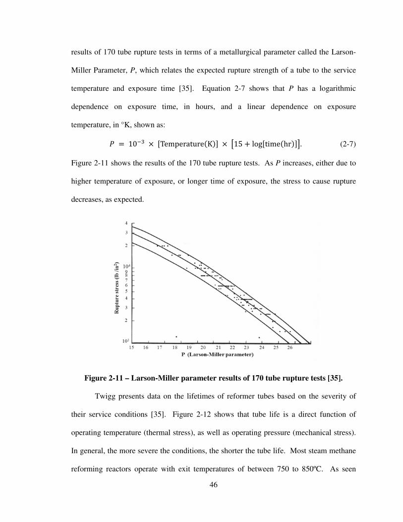
46
results of 170 tube rupture tests in terms of a metallurgical parameter called the Larson-
Miller Parameter, P, which relates the expected rupture strength of a tube to the service
temperature and exposure time [35]. Equation 2-7 shows that P has a logarithmic
dependence on exposure time, in hours, and a linear dependence on exposure
temperature, in °K, shown as:
� = 10�� × Temperature� K�� × �15 + logtime�hr���. (2-7)
Figure 2-11 shows the results of the 170 tube rupture tests. As P increases, either due to
higher temperature of exposure, or longer time of exposure, the stress to cause rupture
decreases, as expected.
Figure 2-11 – Larson-Miller parameter results of 170 tube rupture tests [35].
Twigg presents data on the lifetimes of reformer tubes based on the severity of
their service conditions [35]. Figure 2-12 shows that tube life is a direct function of
operating temperature (thermal stress), as well as operating pressure (mechanical stress).
In general, the more severe the conditions, the shorter the tube life. Most steam methane
reforming reactors operate with exit temperatures of between 750 to 850ºC. As seen
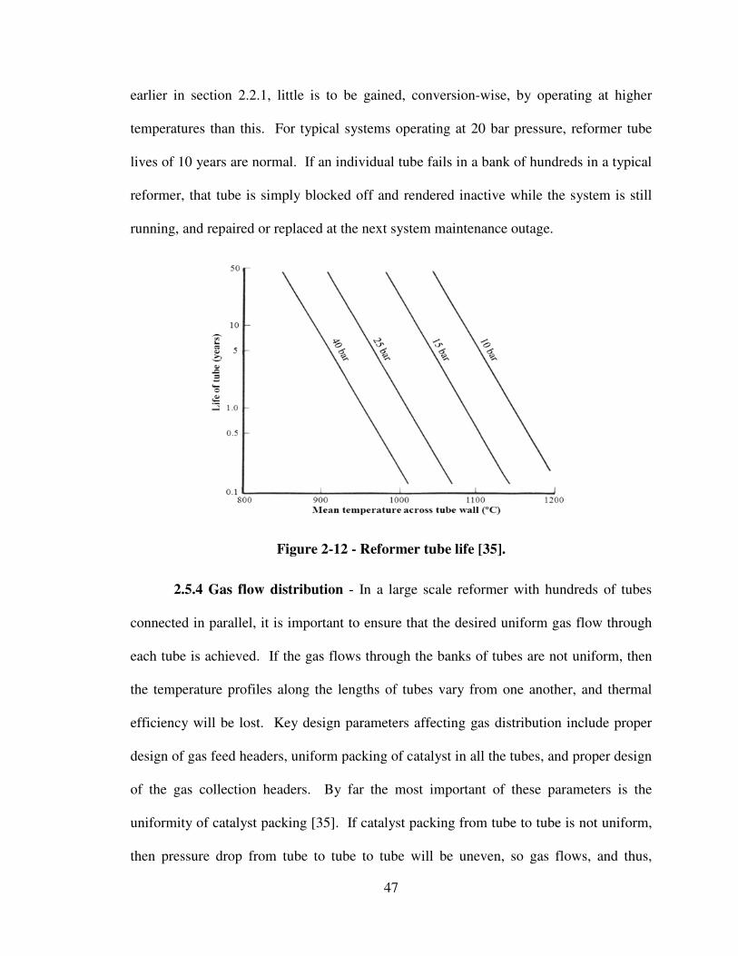
47
earlier in section 2.2.1, little is to be gained, conversion-wise, by operating at higher
temperatures than this. For typical systems operating at 20 bar pressure, reformer tube
lives of 10 years are normal. If an individual tube fails in a bank of hundreds in a typical
reformer, that tube is simply blocked off and rendered inactive while the system is still
running, and repaired or replaced at the next system maintenance outage.
Figure 2-12 - Reformer tube life [35].
2.5.4 Gas flow distribution - In a large scale reformer with hundreds of tubes
connected in parallel, it is important to ensure that the desired uniform gas flow through
each tube is achieved. If the gas flows through the banks of tubes are not uniform, then
the temperature profiles along the lengths of tubes vary from one another, and thermal
efficiency will be lost. Key design parameters affecting gas distribution include proper
design of gas feed headers, uniform packing of catalyst in all the tubes, and proper design
of the gas collection headers. By far the most important of these parameters is the
uniformity of catalyst packing [35]. If catalyst packing from tube to tube is not uniform,
then pressure drop from tube to tube to tube will be uneven, so gas flows, and thus,
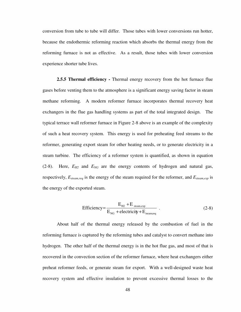
48
conversion from tube to tube will differ. Those tubes with lower conversions run hotter,
because the endothermic reforming reaction which absorbs the thermal energy from the
reforming furnace is not as effective. As a result, those tubes with lower conversion
experience shorter tube lives.
2.5.5 Thermal efficiency - Thermal energy recovery from the hot furnace flue
gases before venting them to the atmosphere is a significant energy saving factor in steam
methane reforming. A modern reformer furnace incorporates thermal recovery heat
exchangers in the flue gas handling systems as part of the total integrated design. The
typical terrace wall reformer furnace in Figure 2-8 above is an example of the complexity
of such a heat recovery system. This energy is used for preheating feed streams to the
reformer, generating export steam for other heating needs, or to generate electricity in a
steam turbine. The efficiency of a reformer system is quantified, as shown in equation
(2-8). Here, EH2 and ENG are the energy contents of hydrogen and natural gas,
respectively, Esteam,req is the energy of the steam required for the reformer, and Esteam,exp is
the energy of the exported steam.
reqsteam,NG
steam,expH2
EyelectricitE
EEEfficiency
++
+
=
. (2-8)
About half of the thermal energy released by the combustion of fuel in the
reforming furnace is captured by the reforming tubes and catalyst to convert methane into
hydrogen. The other half of the thermal energy is in the hot flue gas, and most of that is
recovered in the convection section of the reformer furnace, where heat exchangers either
preheat reformer feeds, or generate steam for export. With a well-designed waste heat
recovery system and effective insulation to prevent excessive thermal losses to the

49
environment, overall thermal energy efficiencies up to 95% can be achieved. However,
smaller-scale systems may not be as efficiently-designed, and typically do not exceed
thermal efficiencies of 60%.
2.5.6 Summary of operation conditions - An overall summary of typical oper-
ating parameters for typical large scale steam methane reformers is included in Table 2-4.
Table 2-4 – Typical operating parameters for a SMR system
PROCESS
STEP
1 2 3 4
Sulfur Removal Reforming Shift
Reactor H2 Purification
Technology
Hydro-
Treatment
S to H2S
H2S
Removal Reforming Water Gas
Pressure
Swing
Adsorption
Pressure
(psig) 440 to 2,000 600 to 1,200 200 to 450 250
200 to 900 in
5 to 70 out
Temperature
(deg C) 340 to 400 760 to 930 260 to 650 30
Catalyst Co-Mo or
Ni-Mo ZnO Ni based Fe-Cr
Mol sieve,
alumina, or silica
gel
Catalyst Life
(years) up to 7 1 to 2 5 5 to 7 Varies
Conversion
or
Efficiency(%)
Varies, depending on Sulfur
load 90 to 95 70 to 75 65 to 90
2.6 Small scale SMR reformer systems
While a full-scale steam methane reforming plant could have as many 650
reformer tubes in its reformer furnace and produce up to 100,000 Nm3hr
-1 of H2, small
users have more modest H2 needs. To meet these, builders of commercial-scale
reformers also offer small systems. Depending on the desired capacity, the number of

50
reformer tubes utilized in such small systems is adjusted as needed to meet the required
H2 output.
2.6.1 Disadvantages of current SMR technology at small scales - Reformer
tubes in a small-scale reformer may number as few as four, but the individual tubes are
the same, dimensionally, as a full-scale commercial reformer. Therefore, they are
approximately 6 to 7 centimeters in diameter and 10 to 12 meters tall, and built from the
same high-temperature alloy steels. Figure 2-13 shows an example of a small-scale, 4-
tube reformer furnace.
Figure 2-13 - Conventional design for small scale steam methane reformers [38].
While the footprint of the reformer furnace is fairly small, the 12 meter height of
the reformer tubes requires significant structural support for the furnace and associated
platforms needed to access the top of the system for maintenance, catalyst loading, etc.
Also, the smaller furnace does not allow for efficient integration of the energy recovery
heat exchangers into the design of the furnace itself, like it does for large-scale reformers.
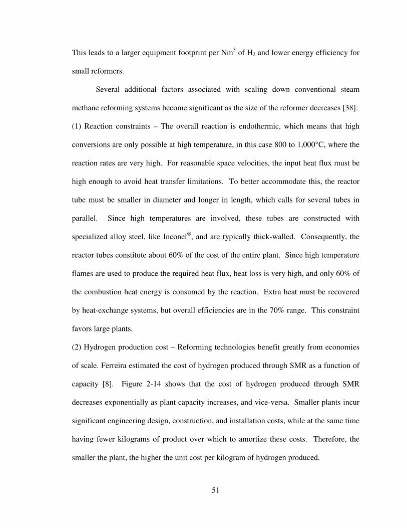
51
This leads to a larger equipment footprint per Nm3 of H2 and lower energy efficiency for
small reformers.
Several additional factors associated with scaling down conventional steam
methane reforming systems become significant as the size of the reformer decreases [38]:
(1) Reaction constraints – The overall reaction is endothermic, which means that high
conversions are only possible at high temperature, in this case 800 to 1,000°C, where the
reaction rates are very high. For reasonable space velocities, the input heat flux must be
high enough to avoid heat transfer limitations. To better accommodate this, the reactor
tube must be smaller in diameter and longer in length, which calls for several tubes in
parallel. Since high temperatures are involved, these tubes are constructed with
specialized alloy steel, like Inconel®
, and are typically thick-walled. Consequently, the
reactor tubes constitute about 60% of the cost of the entire plant. Since high temperature
flames are used to produce the required heat flux, heat loss is very high, and only 60% of
the combustion heat energy is consumed by the reaction. Extra heat must be recovered
by heat-exchange systems, but overall efficiencies are in the 70% range. This constraint
favors large plants.
(2) Hydrogen production cost – Reforming technologies benefit greatly from economies
of scale. Ferreira estimated the cost of hydrogen produced through SMR as a function of
capacity [8]. Figure 2-14 shows that the cost of hydrogen produced through SMR
decreases exponentially as plant capacity increases, and vice-versa. Smaller plants incur
significant engineering design, construction, and installation costs, while at the same time
having fewer kilograms of product over which to amortize these costs. Therefore, the
smaller the plant, the higher the unit cost per kilogram of hydrogen produced.
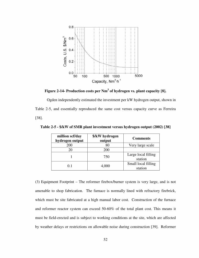
52
Figure 2-14- Production costs per Nm3 of hydrogen vs. plant capacity [8].
Ogden independently estimated the investment per kW hydrogen output, shown in
Table 2-5, and essentially reproduced the same cost versus capacity curve as Ferreira
[38].
Table 2-5 - $/kW of SMR plant investment versus hydrogen output (2002) [38]
million scf/day
hydrogen output
$/kW hydrogen
output Comments
200 80 Very large scale
20 200
1 750 Large local filling
station
0.1 4,000 Small local filling
station
(3) Equipment Footprint – The reformer firebox/burner system is very large, and is not
amenable to shop fabrication. The furnace is normally lined with refractory firebrick,
which must be site fabricated at a high manual labor cost. Construction of the furnace
and reformer reactor system can exceed 50-60% of the total plant cost. This means it
must be field-erected and is subject to working conditions at the site, which are affected
by weather delays or restrictions on allowable noise during construction [39]. Reformer
53
tubes, 10 meters long, require enclosures at least 3 stories high. Although the furnace is
insulated with firebrick or fiber insulation to preserve thermal energy, percentage energy
losses as a function of the amount of active working catalyst are considerably larger for
smaller units because they have a larger furnace wall surface area to catalyst volume ratio
than a large system. This is another of the reasons why a small system cannot achieve the
energy efficiencies of a large system.
(4) Complex burner systems – Combustion systems, operating at low pressure and
featuring radiant heat transfer from the furnace walls lined with firebrick, typically
require large internal dimensions to adequately channel the hot furnace gases around the
tubes and properly expose the tubes to the thermal radiation from the firebrick. Such
structures are costly to build, are thermally inefficient because the large external wall
surfaces create significant energy losses, and the high thermal inertia of a solid wall of
firebrick is difficult to control, temperature-wise. The design of burner systems to
achieve optimum flux profiles along the tube length, and respond to migration of the
active catalytic zone along the reformer tube is difficult to implement. For a small 4-tube
reformer system, it may not be justified to install a sophisticated multi-level burner
system to optimize the catalyst conversion, so its operating efficiency will not be as high
as a large commercial-scale reformer furnace.
(5) Complicated process control - Large flame-fired furnaces require large control
systems to operate efficiently. The complex relationship between catalyst activity and
thermal energy input flux to the tube at the active catalytic zone leads to difficulties in
adjusting burner conditions to follow changes in (a) catalyst activity, (b) flow rate, and
(c) inlet temperature. The inability to reasonably maintain control of the thermal energy
54
flux profiles into the reformer tube in small reformer systems further results in inefficient
operation, poor product quality (inadequate conversion), tube overheating leading to
shorter tube life, and catalyst deactivation. These factors all contribute to the lower
efficiency and higher cost per kg. of H2 associated with smaller reformer systems.
(6) Slow start-up and control response – Furnaces, with their brick-lined walls, have high
thermal inertia which take extended times to heat up to operating temperature. Once up
to operating temperature, this same high thermal inertia leads to control difficulties due to
slow response times to control inputs by the operator, particularly during startup. A cold
restart can last over 24 hours, and even a hot restart can last 6 hours or more. The risk in
having sluggish responses to control inputs is that it could lead to overshooting process
conditions, resulting in damage to the catalyst or to the reformer tubes. To ensure that
startups do not take any longer than necessary, it is important to utilize experienced
operators, if furnace and reactor damage is to be avoided. The most critical period during
any given startup is when the feedstock is introduced. Reformer tubes warm up to red
heat with only steam flowing through the tubes, since the heat sink of the endothermic
reforming reaction has not yet started. In order to achieve a steady temperature rise as
feedstock is introduced, the thermal flux to the reformer tube must be significantly
increased as the methane is introduced to allow for the cooling effect once the reforming
reaction commences. If there are any delays in introducing the methane feed stock when
the heat is turned up on the reformer tubes, disastrous overheating and damage to the
tubes will result. During a startup, before the methane is introduced, and the reformer
tubes are already red hot, it is not difficult to accidentally apply excess burner energy and
overheat the tubes, so caution and experience is required.

55
(7) Low energy recovery – As discussed earlier the combustion process in the furnace
applies only about half of its thermal energy to the reformer tubes. The remaining
thermal energy in the hot flue gas must be recovered or wasted. Large reforming plants
are able to efficiently recover most of the energy in the flue gas, and therefore are able to
realize thermal efficiencies as high as 95%. Small sized plants are not as efficient in this
area. For example, there may not be a use for export steam in a small reformer system.
Therefore, that energy may be wasted. Another reason cited earlier is that the furnace
wall surface to volume ratio for small reformers is larger, resulting in higher thermal
energy losses to the environment compared to a large scale reformer. It is for these
reasons that the maximum efficiency for small scale reformers has been limited to 60 -
70%.
(8) Air pollution, as mentioned before, arises from both NOx formation in the flame-fired
furnaces of existing SMR systems due to the high operating temperatures of the flame-
fired furnaces, and from higher emission of greenhouse gases (CO2) from combustion of
fossil fuels because efficiencies are lower.
2.6.2 Desired characteristics of small-scale reformers - Areas in which con-
ventional small-scale reformer systems need improvement in order to facilitate more
widespread implementation of this technology are as follows;
(1) Reduced size of reactors. Modular construction, capable of being fabricated in a shop
as opposed to field erection, decreases construction costs. Standardized interchangeable
parts, that may be swapped in and out as needed, instead of customized purpose-built
parts, decrease operating and maintenance expenses. Eliminating the 12 meter long
56
reformer tubes for much smaller reactors also significantly reduces the cost of the
required supporting structure for the system.
(2) Increased burner transfer duty and process efficiency. If application of thermal
energy in present reformer furnaces to the reformer tubes is significantly increased over
50%, then there is less dependence on the convective heat recovery of the hot flue gases,
particularly in cases where there is no market for export steam. This increases the overall
thermal energy utilization and overall energy efficiency.
(3) Reduced maintenance and direct operator supervision. Improvements in this area
directly reduce maintenance expense, while less operator supervision reduces the cost of
operating labor, as the operators are tasked to perform additional duties. Reliability also
improves, as there is less opportunity for operator error to cause damage to the
equipment.
(4) Rapid, fully automatic start-up and shut-down. Improvements in this area raise the
system reliability and also reduce the chances of operator errors causing equipment
damage or reductions in reformer tube life.
(5) Decreased noise and environmental emissions. If small reformer systems proliferate,
some may be installed in non-industrial residential areas, which are not tolerant of
significant industrial pollution. Public acceptance of these systems could hinge upon
their having a negligible environmental footprint in the community.
(6) Lower maintenance and repair costs from tube failure. As mentioned above,
automated control systems for startup, shutdown, and normal operation improves
reliability of a small reformer system and maximizes the life of the reformer tubes and
the catalyst within.

57
2.7 Hydrogen production research at the University of Houston
The University of Houston has conducted research into novel compact steam
reformers since 1980. This work, under the direction of Professor James T. Richardson,
has resulted in 18 Ph.D and 12 MSChe degrees and 30 journal publications.
Various aspects of reaction engineering, catalyst supports, and heat transfer have
been studied in research programs such as the following:
(1) mechanisms and kinetics for reduction of nickel-based reforming catalysts.
(2) novel catalysts for carbon-free reforming with CO2 instead of H2O
(3) compact close-coupled steam reforming reactors based on heat pipe technology for
solar heated, as well as fired-heater applications
(4) foamed ceramic catalyst supports with superior mass and heat transfer properties.
(5) novel reforming catalyst structures for solar receivers using steam reforming to store
solar energy.
(6) Catalysis of the detoxification of chlorinated solvent wastes using steam reforming
technology.
(7) Catalytic combustion systems for use in reformers instead of open-flame furnaces.
The background, previous work, and pertinence of three major research areas to
the current study will now be explored. Those three focus area are, (1) heat pipes, (2)
ceramic foam catalyst supports, and (3) catalytic combustion.
2.8 Heat pipes
A heat pipe is an efficient heat transfer device that transports thermal energy from
one location to another by convection of a working fluid through a small cross-sectional
area without additional power input to the system. It utilizes an evacuated sealed

58
container, a wicking structure, and a small amount of working fluid which is in
equilibrium with its own vapor. Heat pipes may be constructed in several different
geometries, including cylindrical tubes, annular tubes, and flat plates. Cylindrical heat
pipes are the most typical configuration, and their operation is described below.
The evaporator section (left side of Figure 2-15), is located at the heat source,
where thermal energy enters the heat pipe and the liquid working fluid evaporates into
vapor, adsorbing the heat of vaporization. Next, the vapor travels through the adiabatic
section of the heat pipe to the condenser section on the right side of Figure 2-16. At the
Figure 2-15 - Schematic of a typical heat pipe showing the principle of operation
and circulation of the working fluid [40].
condenser section, heat is rejected, and the working fluid condenses, giving up its heat of
vaporization. A wick structure connects the condensing and evaporating sections of the
heat pipe, so capillary action conducts the condensed fluid from the condensing section
back to the evaporating section, to start the cycle anew. Because the wick structure takes
advantage of capillary action, a heat pipe does not rely on gravity to transport the
condensed working fluid from the condensing section to the evaporating section, and is
not constrained to operate in the vertical position.
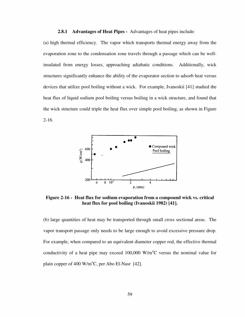
59
2.8.1 Advantages of Heat Pipes - Advantages of heat pipes include:
(a) high thermal efficiency. The vapor which transports thermal energy away from the
evaporation zone to the condensation zone travels through a passage which can be well-
insulated from energy losses, approaching adiabatic conditions. Additionally, wick
structures significantly enhance the ability of the evaporator section to adsorb heat versus
devices that utilize pool boiling without a wick. For example, Ivanoskii [41] studied the
heat flux of liquid sodium pool boiling versus boiling in a wick structure, and found that
the wick structure could triple the heat flux over simple pool boiling, as shown in Figure
2-16.
Figure 2-16 - Heat flux for sodium evaporation from a compound wick vs. critical
heat flux for pool boiling (Ivanoskii 1982) [41].
(b) large quantities of heat may be transported through small cross sectional areas. The
vapor transport passage only needs to be large enough to avoid excessive pressure drop.
For example, when compared to an equivalent diameter copper rod, the effective thermal
conductivity of a heat pipe may exceed 100,000 W/moC versus the nominal value for
plain copper of 400 W/moC, per Abo El-Nasr [42].
60
(c) No additional power input is required. The phase changes occurring at the evap-
oration and condensation zones are entirely driven by the external applied energy, in both
the positive and negative directions of heat flux. Transport of vapor to the condensation
zones is driven by vapor pressure within the heat pipe, and the transport of liquid in the
wick structure from the condensation to the evaporation zones is driven by capillary
pressure, even against gravity, if needed.
(d) Easy control of heat flux, and high rates of heat conduction, even with small changes
in temperature. This benefit arises from the heat pipe’s capacity to adsorb and evaporate
more liquid working fluid in the evaporation zone to accommodate momentary transient
rises in heat input. In such instances, more working fluid gets vaporized quickly enough
to prevent a hot spot from developing in the evaporation section, thus avoiding significant
swings in the temperature. It is not a constant-temperature boiling situation of the
working fluid, because boiling within the heat pipe’s evaporation zone is actually
detrimental to its operation, as will be discussed below. Rather, it is a narrow temp-
erature range evaporation situation that occurs within a heat pipe.
(e) Isothermal conditions along its length – The working fluid is maintained at a specific
pressure inside the tube and it only vaporizes at the corresponding vaporization
temperature. Because of the vapor liquid equilibrium, near-isothermal temperature is
maintained throughout the tube. The evaporation zone temperature and condensation
zone temperature in a heat pipe is so close to each other so as to approximate isothermal
operation.
(f) Decoupling of the heating and cooling sections – Heat pipes allow for individual
geometric separation and optimization of the heating and cooling flux profiles.
61
2.8.2 Choice of working fluid - The choice of working fluids for the heat pipe
depends on matching these two main factors; (1) the temperature range of the operating
system, and, (2), the melting and boiling points of the candidate fluids under consider-
ation. If the temperature at the evaporator end of the heat pipe is too low (lower than the
melting point of the fluid), then the heat pipe only sublimates the solidified fluid, and
never generates enough transfer of heat to attain viable operation. On the other hand, if
the condensing end of the heat pipe is too high in temperature of the candidate working
fluid, then the fluid never condenses and the heat pipe will not work. In practice, the
selection of working fluid is usually well within these limits, shown diagrammatically as;
Tmelting < Operating range of the working fluid < Tboiling. (2-9)
Chapman provided an analysis of the liquid transport through the wick of the heat
pipe from condenser end to the evaporator end [44]. He arrived at an energy flux
equation to represent the flow of heat that represents the upper limit of the heat pipe to
convey heat based on the ability of the wick to pump liquid working fluid (called the
“pumping limit”);
max
21 cos
2
l l
l
gAKq
rL
σρ λ ρβ
µ σ
= × × −
, (2-10)
where A = X-sectional area of wick available for liquid flow (m2)
K = Darcy working fluid permeability of the wick material (m2)
r = Radius of the heat pipe tube (m)
L = Length of the heat pipe (m)
σ = Surface tension of the working fluid (N/m)
ρl = Density of the liquid phase of the working fluid (kg/m3)
62
λ = Latent heat of the working fluid (kcal/kg)
µl = Viscosity of the liquid working fluid (N·s/m2)
g = Gravitational acceleration (m/s2)
β = Angle of the heat pipe from true vertical (radians) .
The first quantity in brackets, 2AK
rL
, depends on the heat pipe geometry and
permeability of the working fluid in the wick material. As such, it is only peripherally
affected by the physical properties of the working fluid, and can be considered almost
constant for a given heat pipe geometry. The second quantity, however, l
l
σρ λ
µ
,
depends significantly on the physical properties of the working fluid. In the flux
equation, 2-10, it can be seen that maximizing this quantity results in maximizing the heat
flux of the heat pipe. Chapman refers to this as the heat pipe liquid transport factor.
If the lower operating limit of the heat pipe operating range is too low (below the
working fluid’s melting point), then its liquid viscosity, µl, goes to infinity and the liquid
transport factor goes to zero. If the upper limit of the heat pipe operating range is too
high (above the working fluid’s boiling temperature), then its latent heat, λ, goes to zero
and the liquid transport factor again goes to zero.
Some examples of metallic working fluids and their operating temperatures are
given in Table 2-6. Metallic sodium and potassium are good candidates for the
temperatures encountered in steam-methane reforming (800 to 1000ºC). Sodium is used
for high temperature heat exchangers and has considerable operating experience. It is
therefore a good choice for steam-methane reformers, although potassium remains a
possible alternative.
63
Table 2-6 – Heat pipe working fluid temperature ranges (Thermacore, Inc.) [28]
Heat Pipe
Working Fluid
Operating
Temperature
Range (ºC)
Cesium 350 to 925
NaK 425 to 825
Potassium 400 to 1,025
Sodium 500 to 1,225
Lithium 925 to 1,825
Silver 1,625 to 2,025
2.8.3 Limitations - Although heat pipes offer many performance advantages over
more conventional heat transfer devices, they are also subject to several design
limitations that can adversely affect their efficiency. The following operational aspects
are overcome with proper design and adequate startup, maintenance, and shutdown
procedures. In some cases, additional equipment is needed, such as startup heaters,
robust thermal insulation, or added vents.
(a) frozen startup limit: If the working fluid within the heat pipe exists as a solid in the
frozen state, then this phenomenon occurs during a startup before the entire heat pipe has
risen up to its normal design operating temperature. During the startup process from the
frozen state, vapor from the evaporation zone may unintentionally condense and freeze in
the adiabatic zone before it has a chance to travel all the way to the normal condensing
zone. In extreme cases, this depletes enough working fluid from the evaporation zone to
cause dry out of the evaporator and cessation of the normal heat pipe evaporating and
condensing cycle. This happens more easily with heat pipes using liquid metal as the
working fluid, before the heat pipe has had a chance to fully warm up to normal operating
temperature. Auxiliary heaters during the startup phase may be required, as well as
adequate thermal insulation of the adiabatic zone, to prevent thermal losses and potential
64
condensation of the vapor from condensing where it is not designed to condense, before it
has a chance to travel all the way to the normal condensing zone. For the liquid sodium
working fluid, the liquid metal melting point of the sodium within the heat pipe is 371ºC,
so proper design and startup procedures are required to ensure successful operation.
(b) viscous limit: If viscous forces dominate the vapor flow of the working fluid, the
delta-p motive force driving the vapor of the working fluid to the condenser end may
reduce to zero. When this happens, heat transfer becomes limited, and the system
behaves similarly to the frozen startup scenario in (a) above. This most often happens in
a liquid-metal heat pipe when the heat pipe is operating below its normal operating range,
or during a startup transient. Again, auxiliary heaters assist with preventing this
limitation when needed. Faghri calculated the theoretical ultimate viscous limit of axial
heat flux density for a sodium heat pipe, and compared it to experimental data, shown in
Figure 2-18 [40]. It is calculated only up to 600°C, but it shows that the viscous limit
curve intersects the sonic limit curve at approximately 550°C. From 550°C on up, the
sonic limit controls the ultimate heat flux attainable with a sodium heat pipe, and not the
viscous limit.
(c) sonic limit: For heat pipes with liquid metal working fluids, the vapor velocity
between the evaporating section to the condensing section may reach sonic velocities,
creating a condition called sonic choking. This is the upper limit for vapor transport from
the evaporator section to the condenser section. In Figure 2-17, Busse calculated the
theoretical ultimate heat flux of a sodium heat pipe, and compared it to experimental data
[44]. The experimental results correlated well with theoretical calculations, and followed
the transition from viscous-controlled flux limits to sonic controlled limits. The meas-
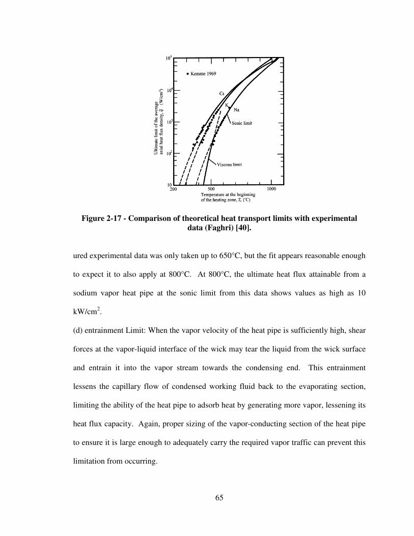
65
Figure 2-17 - Comparison of theoretical heat transport limits with experimental
data (Faghri) [40].
ured experimental data was only taken up to 650°C, but the fit appears reasonable enough
to expect it to also apply at 800°C. At 800°C, the ultimate heat flux attainable from a
sodium vapor heat pipe at the sonic limit from this data shows values as high as 10
kW/cm2.
(d) entrainment Limit: When the vapor velocity of the heat pipe is sufficiently high, shear
forces at the vapor-liquid interface of the wick may tear the liquid from the wick surface
and entrain it into the vapor stream towards the condensing end. This entrainment
lessens the capillary flow of condensed working fluid back to the evaporating section,
limiting the ability of the heat pipe to adsorb heat by generating more vapor, lessening its
heat flux capacity. Again, proper sizing of the vapor-conducting section of the heat pipe
to ensure it is large enough to adequately carry the required vapor traffic can prevent this
limitation from occurring.

66
(e) capillary limit: For a given wick structure and working fluid combination, the
pumping ability of the capillary structure to provide the needed circulation of condensate
has an upper limit. If the capillary flow of liquid from the condenser section to the
evaporator is inadequate, the evaporator section dries out, stopping the flow of heat.
Another name for this is the hydrodynamic limit. This limit is avoided with proper
design and size of the wick structure and orientation. The design criteria is expressed in
terms of pressure drop as
∆pcap,max ≥ ∆pl + ∆pv + ∆pe,δ + ∆pc,δ + ∆pg , (2.11)
where
∆pcap,max is the maximum capillary head,
∆pl is the pressure drop of the liquid flow in a wick structure from frictional drag,
∆pv is the vapor pressure drop along the heat pipe,
∆pe,δ is the pressure drop due to evaporation at the liquid/vapor interface,
∆pc,δ is the pressure drop due to condensation at the liquid/vapor interface, and
∆pg is the pressure drop in the liquid due to gravity along the heat pipe axis.
Figure 2-18 shows how these 6 parameters interact with each other and define
pressure balance and operating envelope in each zone of a given heat pipe [40].
(f) condenser limit: The maximum heat removal rate of the heat pipe is limited by the
cooling ability of the condenser, either by inadequate heat transfer area, or lack of driving
force (i.e., low delta-temperature). Proper design factors must be applied to avoid
encountering this limitation. Another factor creating this limitation is the presence of
non-condensable gas in the heat pipe. A non-condensable gas in the heat pipe arises from
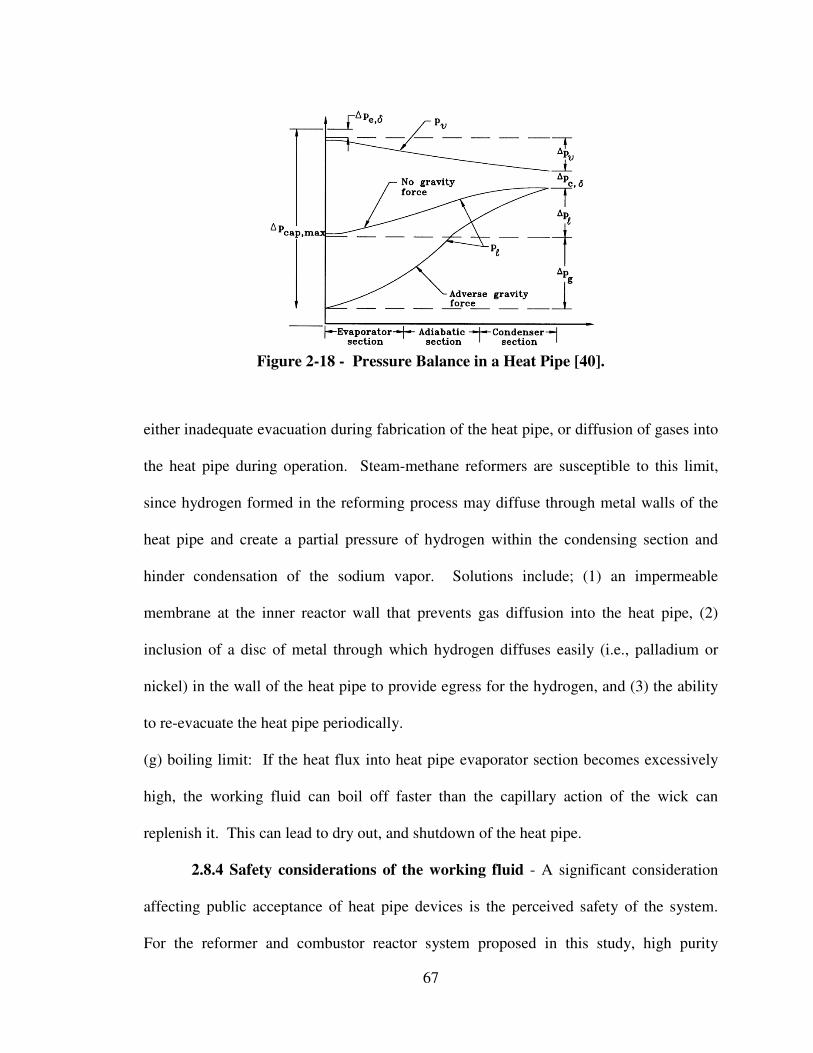
67
Figure 2-18 - Pressure Balance in a Heat Pipe [40].
either inadequate evacuation during fabrication of the heat pipe, or diffusion of gases into
the heat pipe during operation. Steam-methane reformers are susceptible to this limit,
since hydrogen formed in the reforming process may diffuse through metal walls of the
heat pipe and create a partial pressure of hydrogen within the condensing section and
hinder condensation of the sodium vapor. Solutions include; (1) an impermeable
membrane at the inner reactor wall that prevents gas diffusion into the heat pipe, (2)
inclusion of a disc of metal through which hydrogen diffuses easily (i.e., palladium or
nickel) in the wall of the heat pipe to provide egress for the hydrogen, and (3) the ability
to re-evacuate the heat pipe periodically.
(g) boiling limit: If the heat flux into heat pipe evaporator section becomes excessively
high, the working fluid can boil off faster than the capillary action of the wick can
replenish it. This can lead to dry out, and shutdown of the heat pipe.
2.8.4 Safety considerations of the working fluid - A significant consideration
affecting public acceptance of heat pipe devices is the perceived safety of the system.
For the reformer and combustor reactor system proposed in this study, high purity

68
metallic sodium best meets the operating temperature range the heat pipe. There are
perceived safety concerns with a heat pipe operating at 800⁰ C with sodium vapor in
close proximity to a feed stream of methane and water vapor.
In the event that the integrity of the heat pipe containment vessel is lost during
operation, the following scenario occurs: air, H2O, CO2, and methane are drawn into the
heat pipe since the normal heat pipe pressure is slightly negative. The resulting reaction
between steam and sodium vapor forms sodium oxide, sodium hydride, and hydrogen
[41],
Na + H2O � NaOH + ½ H2, (2-12)
2 Na + H2O � Na2O + NaH, (2-13)
NaH � Na + ½ H2. (2-14)
The reactions progress as long as the external pressure outside the heat pipe is higher than
the internal pressure and continues to drive steam into the interior of the heat pipe. As
hydrogen forms within the heat pipe by reaction of the steam with sodium, the internal
pressure rises and eventually balances the external pressure. At this point, further
reaction (and pressure rise within the heat pipe) comes to a halt, and the reformer system
shuts down. The majority of the sodium within the heat pipe remains unreacted, and
there is no catastrophic rupture of the heat pipe vessel due to uncontrolled reaction of the
sodium with the steam.
Zhang and Zhuang conducted simulations of heat pipe ruptures in the condensing
sections of sodium heat pipes used as heat exchangers for steam generation and found
similar results [45]. Such an event occurs in two phases: (1) an initial intensely rapid
reaction, characterized as a quantitative sodium-steam reaction in the limited volume of

69
the heat pipe that increases the internal pressure of the heat pipe, and (2) equalization of
the internal and external pressures, slowing any further reaction by orders of magnitude
than the initial phase, since further steam intrusion into the heat pipe is minimized by the
hydrogen partial pressure generated inside the heat pipe.
Reid et al., of Los Alamos National laboratory also conducted heat pipe failure
tests in which they injected water into sodium heat pipes through openings in the heat
pipe vessel from 0.25 mm to 4.80 mm in diameter [46,47]. They found that the external
pressure outside the heat pipe driving water or steam into the heat pipe was the main
determinant of the extent of the reaction as to how much sodium was reacted in a breach
of the heat pipe vessel. Table 2-7 shows that, in experiment 5, even with the largest
opening, and driven by a pressure of pressure of 2,000 kPa (290 psia), the actual extent of
reaction of the available sodium within the heat pipe was less than 10%, as determined by
the amount of heat released. In parallel with these experiments, Reid derived an energy
balance relation as a predictive tool to estimate the extent of reaction and temperature rise
of a sodium heat pipe breach [47]. Experiments 1 through 5 in Table 2-7 were compared
to this predictive tool, and the goodness of fit between the predicted temperature rise and
the observed temperature rise for tests 1 through 5 were reasonably close, as can be seen
in Figure 2-19.
Encouraged by these results, Reid used this predictive tool to calculate how high
an external pressure would be required to force enough steam into the heat pipe to react
all of the sodium to completion. Row 6 of Table 2-7 is the result of that calculation,
showing that it would require an external pressure of 40,000 kPa (5,800 psia). With all of
the sodium reacted in row 6, the internal pressure would then be adequate to overcome
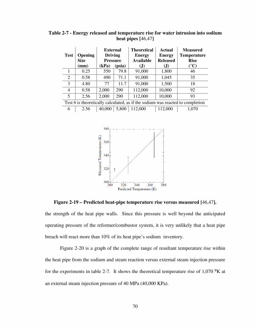
70
Table 2-7 - Energy released and temperature rise for water intrusion into sodium
heat pipes [46,47]
Test
Opening
Size
(mm)
External
Driving
Pressure
(kPa) (psia)
Theoretical
Energy
Available
(J)
Actual
Energy
Released
(J)
Measured
Temperature
Rise
(°C)
1 0.25 550 79.8 91,000 1,800 46
2 0.58 490 71.1 91,000 1,045 35
3 4.80 77 11.7 91,000 1,500 18
4 0.58 2,000 290 112,000 10,000 92
5 2.56 2,000 290 112,000 10,000 93
Test 6 is theoretically calculated, as if the sodium was reacted to completion
6 2.56 40,000 5,800 112,000 112,000 1,070
Figure 2-19 – Predicted heat-pipe temperature rise versus measured [46,47].
the strength of the heat pipe walls. Since this pressure is well beyond the anticipated
operating pressure of the reformer/combustor system, it is very unlikely that a heat pipe
breach will react more than 10% of its heat pipe’s sodium inventory.
Figure 2-20 is a graph of the complete range of resultant temperature rise within
the heat pipe from the sodium and steam reaction versus external steam injection pressure
for the experiments in table 2-7. It shows the theoretical temperature rise of 1,070 ⁰K at
an external steam injection pressure of 40 MPa (40,000 KPa).
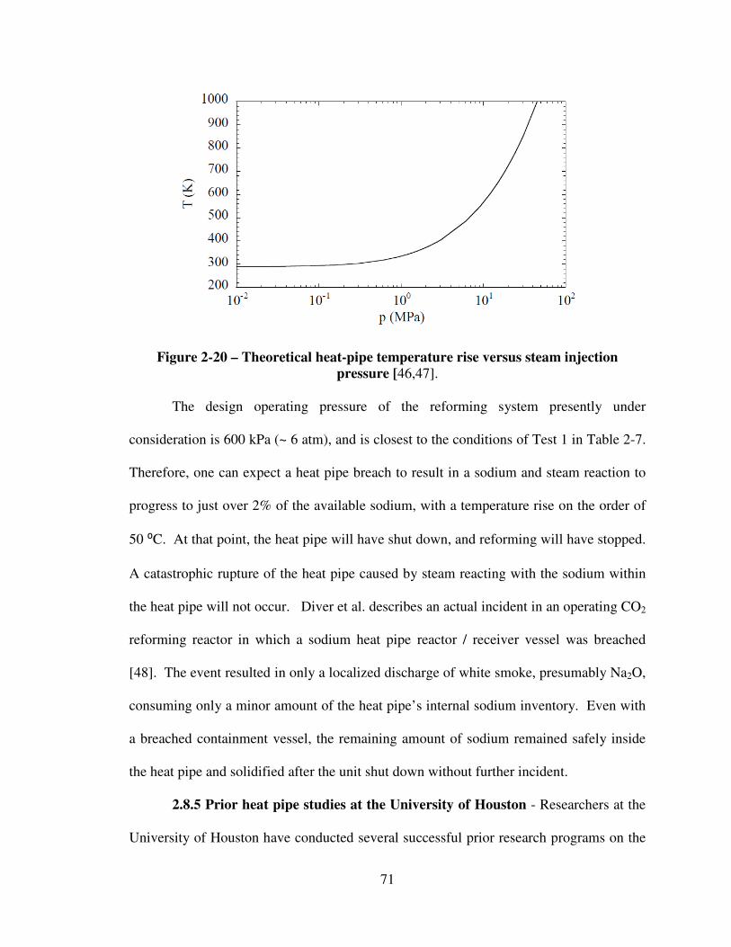
71
Figure 2-20 – Theoretical heat-pipe temperature rise versus steam injection
pressure [46,47].
The design operating pressure of the reforming system presently under
consideration is 600 kPa (~ 6 atm), and is closest to the conditions of Test 1 in Table 2-7.
Therefore, one can expect a heat pipe breach to result in a sodium and steam reaction to
progress to just over 2% of the available sodium, with a temperature rise on the order of
50 ⁰C. At that point, the heat pipe will have shut down, and reforming will have stopped.
A catastrophic rupture of the heat pipe caused by steam reacting with the sodium within
the heat pipe will not occur. Diver et al. describes an actual incident in an operating CO2
reforming reactor in which a sodium heat pipe reactor / receiver vessel was breached
[48]. The event resulted in only a localized discharge of white smoke, presumably Na2O,
consuming only a minor amount of the heat pipe’s internal sodium inventory. Even with
a breached containment vessel, the remaining amount of sodium remained safely inside
the heat pipe and solidified after the unit shut down without further incident.
2.8.5 Prior heat pipe studies at the University of Houston - Researchers at the
University of Houston have conducted several successful prior research programs on the
72
use of sodium heat pipes in steam reforming. Richardson et al. studied a 230 cm long by
5.1 cm diameter sodium heat pipe operating at 825°C, which was designed to convey up
to 20 kilowatts (kW) of thermal energy supplied by electrical heaters to a steam-methane
reforming reactor [49]. Figure 2-21 shows the layout of the heat pipe in the pilot plant.
The cylindrical heat pipe is centrally located, and infrared radiant heaters feed thermal
energy into the bottom end (evaporation zone). The liquid sodium is vaporized from the
bottom evaporator section, and the sodium vapor travels vertically upward to condense in
the upper condensing section and release its latent heat of vaporization to the packed bed
reactor surrounding the heat pipe. Although the heat pipe was rated for operation at
greater than 20 kW of delivered thermal energy, other equipment limitations in the pilot
plant kept the delivered power to 6 kW. An important issue encountered in the pilot plant
reformer testing was infiltration of hydrogen gas from the reforming reaction into the
central chamber of the heat pipe. Hydrogen diffusion through metals, even through the
Inconel®
high-temperature alloy used in the heat pipe, is a well-known phenomenon, as
described by Robertson [50]. As the hydrogen diffused through the wall of the pilot plant
heat pipe, it added to and increased the internal pressure inside the heat pipe. Eventually,
the added partial pressure of the hydrogen inside the heat pipe hindered the effective
condensation of sodium vapor in the condenser section. Thus, it failed to deliver the full
heat load to the reformer, significantly affecting its heat transfer performance. The extent
of permeation was measured over time to quantify the rate at which it occurred, as shown
in Figure 2-22. The permeation rate was approximately 400 cm3 of hydrogen (at STP)
over 20 days of operation. The cylindrical surface area exposed to hydrogen in the
reformer was approximately 180 cm long by 6 cm in diameter, or 3,393 cm2, yielding an
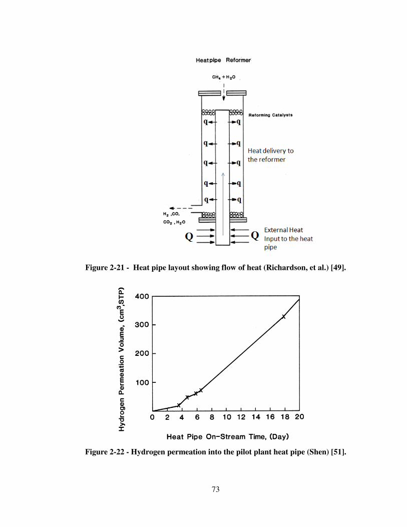
73
Figure 2-21 - Heat pipe layout showing flow of heat (Richardson, et al.) [49].
Figure 2-22 - Hydrogen permeation into the pilot plant heat pipe (Shen) [51].
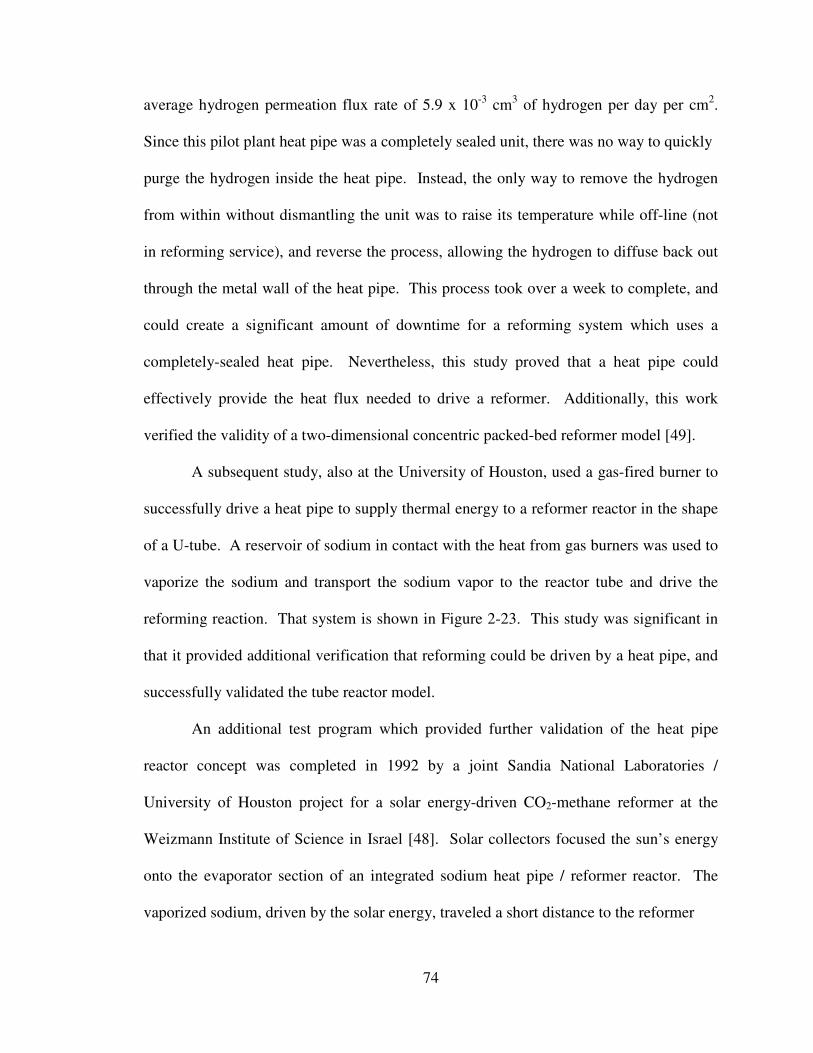
74
average hydrogen permeation flux rate of 5.9 x 10⁻³
cm3 of hydrogen per day per cm
2.
Since this pilot plant heat pipe was a completely sealed unit, there was no way to quickly
purge the hydrogen inside the heat pipe. Instead, the only way to remove the hydrogen
from within without dismantling the unit was to raise its temperature while off-line (not
in reforming service), and reverse the process, allowing the hydrogen to diffuse back out
through the metal wall of the heat pipe. This process took over a week to complete, and
could create a significant amount of downtime for a reforming system which uses a
completely-sealed heat pipe. Nevertheless, this study proved that a heat pipe could
effectively provide the heat flux needed to drive a reformer. Additionally, this work
verified the validity of a two-dimensional concentric packed-bed reformer model [49].
A subsequent study, also at the University of Houston, used a gas-fired burner to
successfully drive a heat pipe to supply thermal energy to a reformer reactor in the shape
of a U-tube. A reservoir of sodium in contact with the heat from gas burners was used to
vaporize the sodium and transport the sodium vapor to the reactor tube and drive the
reforming reaction. That system is shown in Figure 2-23. This study was significant in
that it provided additional verification that reforming could be driven by a heat pipe, and
successfully validated the tube reactor model.
An additional test program which provided further validation of the heat pipe
reactor concept was completed in 1992 by a joint Sandia National Laboratories /
University of Houston project for a solar energy-driven CO2-methane reformer at the
Weizmann Institute of Science in Israel [48]. Solar collectors focused the sun’s energy
onto the evaporator section of an integrated sodium heat pipe / reformer reactor. The
vaporized sodium, driven by the solar energy, traveled a short distance to the reformer
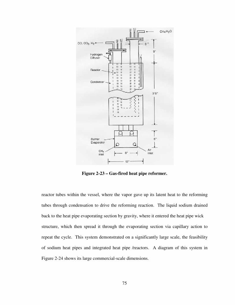
75
Figure 2-23 – Gas-fired heat pipe reformer.
reactor tubes within the vessel, where the vapor gave up its latent heat to the reforming
tubes through condensation to drive the reforming reaction. The liquid sodium drained
back to the heat pipe evaporating section by gravity, where it entered the heat pipe wick
structure, which then spread it through the evaporating section via capillary action to
repeat the cycle. This system demonstrated on a significantly large scale, the feasibility
of sodium heat pipes and integrated heat pipe /reactors. A diagram of this system in
Figure 2-24 shows its large commercial-scale dimensions.

76
Figure 2-24 – 20 kW Sandia-Israel reflux heat-pipe receiver/reactor [48].
2.9 Ceramic foam catalyst supports
Richardson, et al., at the University of Houston, have studied and tested
reticulated ceramic foams as an alternative to the current extruded or pelleted thick ring
catalyst supports for steam methane reforming [52-60]. These sponge-like substrates
feature (1) high surface area for depositing a washcoat of active catalyst, (2) low
resistance to fluid flow, and (3) tortuous flow paths, enhancing turbulence mixing and
improved heat and mass transfer [53-55].

77
Ceramic foam catalyst substrates are prepared using the steps outlined in Figure
2-25. (1) Starting with a block of open-cell polyurethane foam, the foam is molded or
shaped to the desired geometrical shape. (2) The foam form is then filled with low-
viscosity slurry of the ceramic precursor, creating a wet foam form. (3) The foam form is
then drained, dried, and calcined, converting the ceramic precursor on the wet foam form
into a positive image of the original starting geometrical shape.
Figure 2-25 - Steps for making a ceramic foam substrate [36].
The variety of ceramic foam geometrical shapes that may be fabricated is limited
only by the ability to shape the starting polyurethane foam. Figure 2-26 shows several
examples of ceramic foam shapes for different applications.
A magnified view of a typical reticulated ceramic foam structure is shown in
Figure 2-27. The inter-connectedness of the flow passages is evident in the open cell
structure, which creates the low pressure drop characteristics of this material, yet the ran-

78
Figure 2-26 - Varietal shapes for ceramic foam substrates [36].
dom placement of the struts, cells, and windows ensure that transverse mixing in a flow
field is enhanced. The ceramic foam substrate is still only a support, and possesses no
Figure 2-27 - Photomicrograph of a reticulated ceramic foam [36].
catalytic properties of its own, and it is produced in various pore densities. Table 2-8
details the property differences between ceramic foam supports with 5 different pore
densities.
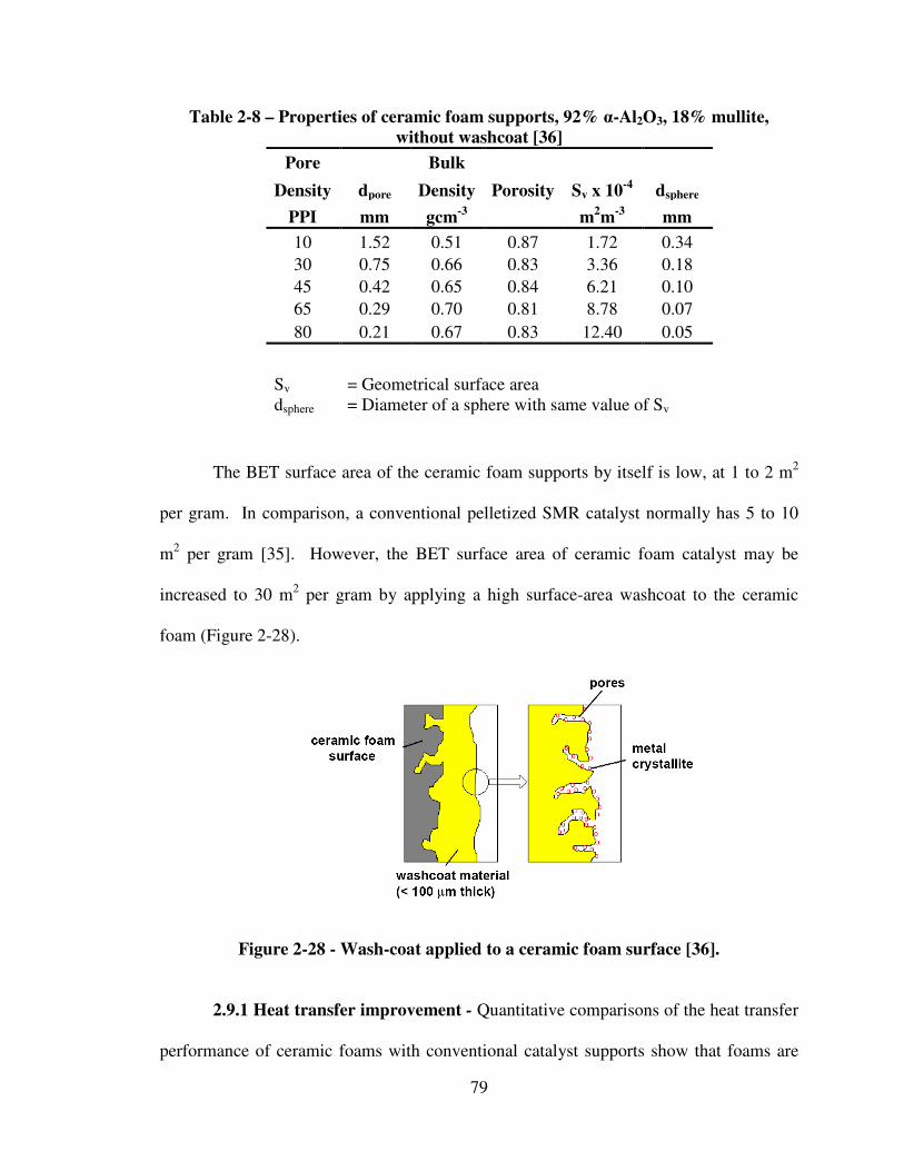
79
Table 2-8 – Properties of ceramic foam supports, 92% α-Al2O3, 18% mullite,
without washcoat [36]
Pore Bulk
Density dpore Density Porosity Sv x 10-4
dsphere
PPI mm gcm-3
m2m
-3 mm
10 1.52 0.51 0.87 1.72 0.34
30 0.75 0.66 0.83 3.36 0.18
45 0.42 0.65 0.84 6.21 0.10
65 0.29 0.70 0.81 8.78 0.07
80 0.21 0.67 0.83 12.40 0.05
Sv = Geometrical surface area
dsphere = Diameter of a sphere with same value of Sv
The BET surface area of the ceramic foam supports by itself is low, at 1 to 2 m2
per gram. In comparison, a conventional pelletized SMR catalyst normally has 5 to 10
m2 per gram [35]. However, the BET surface area of ceramic foam catalyst may be
increased to 30 m2 per gram by applying a high surface-area washcoat to the ceramic
foam (Figure 2-28).
Figure 2-28 - Wash-coat applied to a ceramic foam surface [36].
2.9.1 Heat transfer improvement - Quantitative comparisons of the heat transfer
performance of ceramic foams with conventional catalyst supports show that foams are
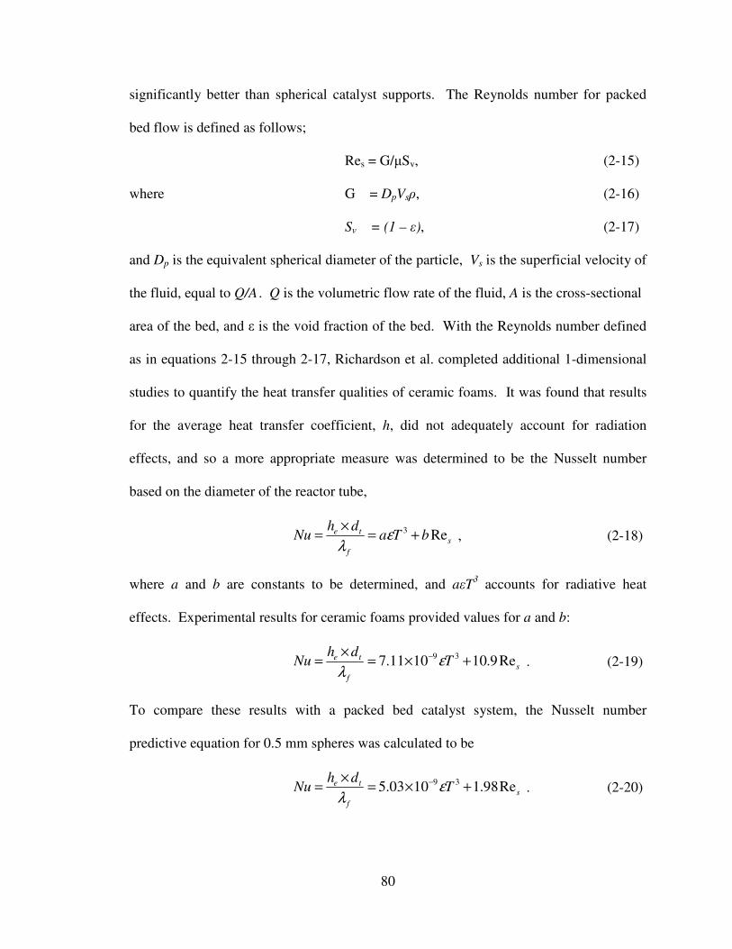
80
significantly better than spherical catalyst supports. The Reynolds number for packed
bed flow is defined as follows;
Res = G/µSv, (2-15)
where G = DpVsρ, (2-16)
Sv = (1 – ε), (2-17)
and Dp is the equivalent spherical diameter of the particle, Vs is the superficial velocity of
the fluid, equal to Q/A . Q is the volumetric flow rate of the fluid, A is the cross-sectional
area of the bed, and ε is the void fraction of the bed. With the Reynolds number defined
as in equations 2-15 through 2-17, Richardson et al. completed additional 1-dimensional
studies to quantify the heat transfer qualities of ceramic foams. It was found that results
for the average heat transfer coefficient, h, did not adequately account for radiation
effects, and so a more appropriate measure was determined to be the Nusselt number
based on the diameter of the reactor tube,
s
f
te bTadh
Nu Re3+=
×= ε
λ
, (2-18)
where a and b are constants to be determined, and aεT3 accounts for radiative heat
effects. Experimental results for ceramic foams provided values for a and b:
s
f
te Tdh
Nu Re9.101011.7 39+×=
×=
−
ε
λ
. (2-19)
To compare these results with a packed bed catalyst system, the Nusselt number
predictive equation for 0.5 mm spheres was calculated to be
s
f
te Tdh
Nu Re98.11003.5 39+×=
×=
−
ε
λ
. (2-20)
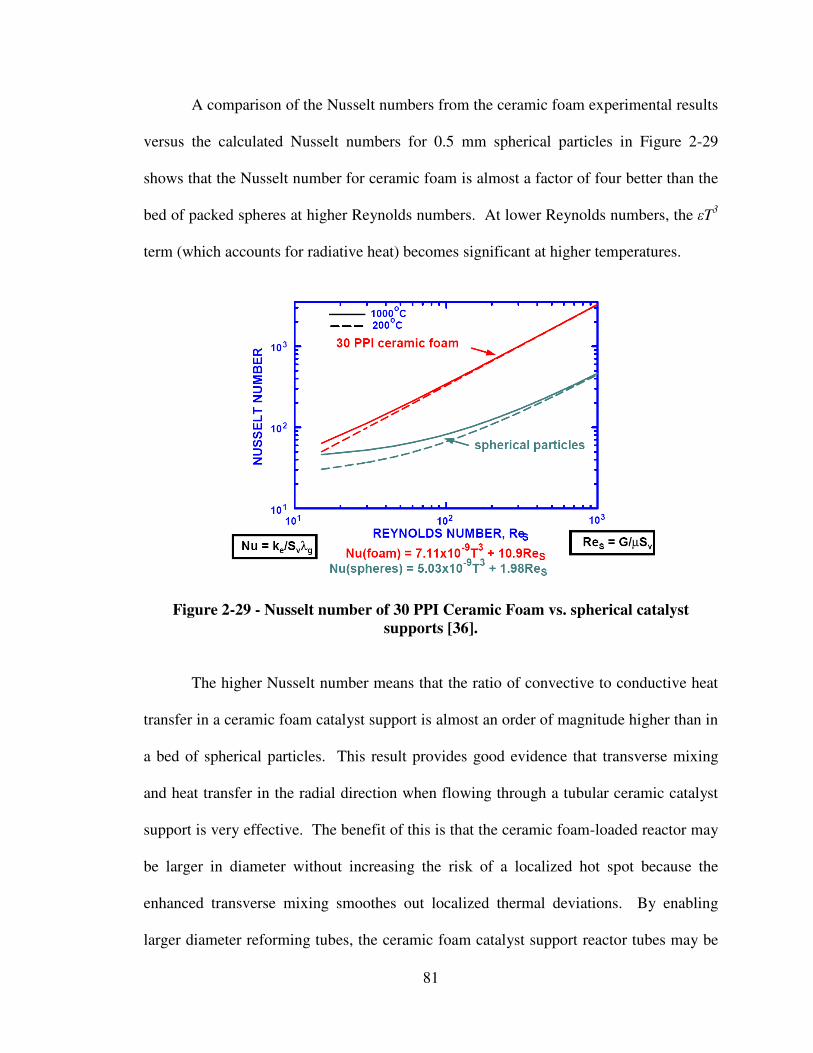
81
A comparison of the Nusselt numbers from the ceramic foam experimental results
versus the calculated Nusselt numbers for 0.5 mm spherical particles in Figure 2-29
shows that the Nusselt number for ceramic foam is almost a factor of four better than the
bed of packed spheres at higher Reynolds numbers. At lower Reynolds numbers, the εT3
term (which accounts for radiative heat) becomes significant at higher temperatures.
Figure 2-29 - Nusselt number of 30 PPI Ceramic Foam vs. spherical catalyst
supports [36].
The higher Nusselt number means that the ratio of convective to conductive heat
transfer in a ceramic foam catalyst support is almost an order of magnitude higher than in
a bed of spherical particles. This result provides good evidence that transverse mixing
and heat transfer in the radial direction when flowing through a tubular ceramic catalyst
support is very effective. The benefit of this is that the ceramic foam-loaded reactor may
be larger in diameter without increasing the risk of a localized hot spot because the
enhanced transverse mixing smoothes out localized thermal deviations. By enabling
larger diameter reforming tubes, the ceramic foam catalyst support reactor tubes may be

82
built with a shorter length than the 10 m of conventional style reformer tubes, allowing
for more compact systems.
Comparing additional thermal parameters of ceramic foams versus other
conventional catalyst supports in the last row of Table 2-9 shows that the effective
thermal conductivity, λe, of ceramic foam is superior to conventional catalyst substrates.
This result provides further confirmation that a ceramic foam catalyst will perform better
at avoiding localized hot spots than conventional catalyst supports by being better able to
dissipate and conduct away excess thermal energy.
Table 2-9 - Comparison of Thermal Parameters of Catalyst Support Structures [36]
The improved heat transfer characteristics of ceramic foam proven in University
of Houston research programs offer design and operating improvements over packed bed
catalyst systems. They can overcome the present dimensional conventions of typical
SMR reformer tubes (100 to 120 mm in diameter and 10 to 12 m in length) so that
ceramic foam reformer reactors may be larger in diameter and shorter in length, enabling
more compact designs to be built. The three areas which are directly improved by

83
ceramic foam catalysts are (1) reduced pressure drop, (2) better mass transfer, and (3)
tailored catalytic activity profiling in the catalyst bed.
2.9.2 Pressure drop improvement - Another advantage that ceramic foam
catalyst supports provide over conventional substrates, such as packed beds of particles,
is reduced pressure drop. Targeted studies by Richardson, et al. in 2000, generated
comparative flow performance data of ceramics foams versus packed beds [53]. Figure
2-30 shows that the comparative pressure drop through a 30 PPI ceramic foam insert is an
order of magnitude less than the pressure drop of a packed bed of 0.5 mm diameter glass
spheres. The lower pressure drop means that auxiliary fluid handling equipment like
piping, valves, pumps, compressors, and blowers to drive the fluid flow through a
ceramic foam catalyst system can be significantly smaller and less costly than for
conventional packed beds.
Figure 2-30 - Comparison of pressure drop for a bed of glass spheres and 30-PPI,
99.5 wt.% α-Al2O3 [53].

84
2.9.3 Mass Transfer Improvement - The mass transfer capabilities of ceramic
foam were studied by Richardson [55]. When 30 PPI ceramic foam was compared to a
conventional packed bed, the mass transfer factor was found to be comparable. Figure 2-
31 shows a colburn plot of Reynolds number versus the mass transfer factor, jD, where
V
Sckj c
D
667.0
= , (2-21)
mDSc
1ρ
µ= , and (2-22)
=mD1 diffusivity of species 1 in the bulk fluid m. (2-23)
The mass transfer coefficient as shown in equation 2-21 can provide a comparison
between the magnitudes of the momentum diffusivity (viscosity), versus the mass
diffusivity. Such a comparison can yield some insight on the controlling mechanism in a
Figure 2-31 - Colburn plot of jD versus Res [55].
reactor system. Small mass transfer factors with a value much smaller than one indicate
that the mass diffusivity dominates over the momentum diffusivity. We say then, that the
system is diffusion controlled, and not viscous controlled. A large mass transfer factor
85
much greater than one indicates that momentum diffusivity dominates over mass
diffusivity, and thus is viscous-controlled.
In Figure 2-31, the B & U upper and lower limits (dashed lines) depict the
boundaries for the mass transfer factor, εjD, as determined for a large number of
representative catalyst particles by Dwivedi and Upadhyay [62]. Measured data for the
mass transfer factor obtained by Richardson [57] for 30 PPI ceramic foam could be
curve-fitted very well on a line with its equation equal to
εjD = 0.223*Res -0.416
. (2-24)
Dwivedi and Upadhyay provided a nominal correlation that summarized all their
data into one general expression,
εjD = 0.455*Res -0.407
. (2-25)
The close similarity between the experimentally-determined mass transfer factor
correlation for 30 PPI ceramic foam in equation 2-24 to the generalized equation by
Dwivedi and Upadhyay in equation 2-25 leads to the conclusion that the mass transfer
characteristics of 30 PPI ceramic foam is at least as effective as for packed beds.
2.10 Catalytic combustion
Catalytic combustion has been evaluated at the University of Houston as a heat
source for a compact steam methane reformer system in place of the traditional open
flame-fired combustion chamber. In a flame-fired combustion chamber of a conventional
reformer system, burning natural gas with air results in extremes in flame temperature of
up to 1700ºC, as seen in Figure 2-33 [63]. In Figure 2-32, the left side depicts the
geometry of a typical terrace wall flame-fired reformer fire box. The right side of this
figure depicts the internal temperature contours modeled using computational flow
86
dynamics. It shows that there are zones within the firebox which exceed 1700ºC. These
Figure 2-32 - Reformer firebox geometry and internal temperature contours [63].
combustion temperatures result in the formation of oxides of nitrogen, a significant air
pollutant, by the reaction of nitrogen and oxygen as in equation 2-26:
N2 + O2 � 2 NO . (2-26)
Figure 2-33 shows how the higher temperatures of open flame combustion at greater than
1300°C exponentially increase the amount of oxides of nitrogen which are produced.
Nitrogen oxide (NOx) emissions contribute to degradation of the environment by playing
a significant role in the production of acid rain, and in the creation of low level ozone in
the air, according to the USEPA (1980) [64].
There are several proven methods for reducing NOx emissions available that may
be applied to current reformer systems. These include such methods such as exhaust gas

87
recirculation to reduce the oxygen concentration in the firebox, similar to the concept
Figure 2-33 - Effect of combustion temperature on oxides of nitrogen creation [36].
applied to automotive internal combustion engines. Other means of NOx reduction
include injection of scavenging chemicals like urea or ammonia to decompose the NOx
once it is formed. But such measures as a whole cut into productivity and efficiency of
the unit, and may also create a different, if not larger environmental issue due to the
introduction of other potentially harmful chemicals to the environment.
One means of avoiding the high combustion temperatures of open flame
combustion and reduce significant amounts of NOx formation is catalytic combustion of
natural gas with air. Instead of exposure to open flame firebox temperatures up to
1,700°C, a catalytic combustor can operate at less than 1,200°C and minimize NOx
formation, because the catalyzed combustion of natural gas and air occurs without a
flame, and is distributed across the catalyst surface. They can also operate at fuel to air
ratios below methane’s lower flammability limits in air, so safety of operation is
enhanced. The model predictions of a typical average axial temperature profile of such a
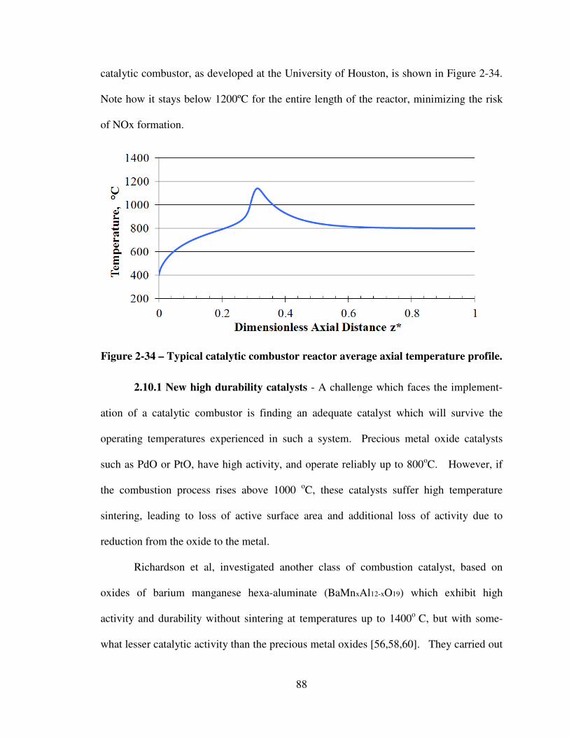
88
catalytic combustor, as developed at the University of Houston, is shown in Figure 2-34.
Note how it stays below 1200ºC for the entire length of the reactor, minimizing the risk
of NOx formation.
Figure 2-34 – Typical catalytic combustor reactor average axial temperature profile.
2.10.1 New high durability catalysts - A challenge which faces the implement-
ation of a catalytic combustor is finding an adequate catalyst which will survive the
operating temperatures experienced in such a system. Precious metal oxide catalysts
such as PdO or PtO, have high activity, and operate reliably up to 800oC. However, if
the combustion process rises above 1000 oC, these catalysts suffer high temperature
sintering, leading to loss of active surface area and additional loss of activity due to
reduction from the oxide to the metal.
Richardson et al, investigated another class of combustion catalyst, based on
oxides of barium manganese hexa-aluminate (BaMnxAl12-xO19) which exhibit high
activity and durability without sintering at temperatures up to 1400o
C, but with some-
what lesser catalytic activity than the precious metal oxides [56,58,60]. They carried out
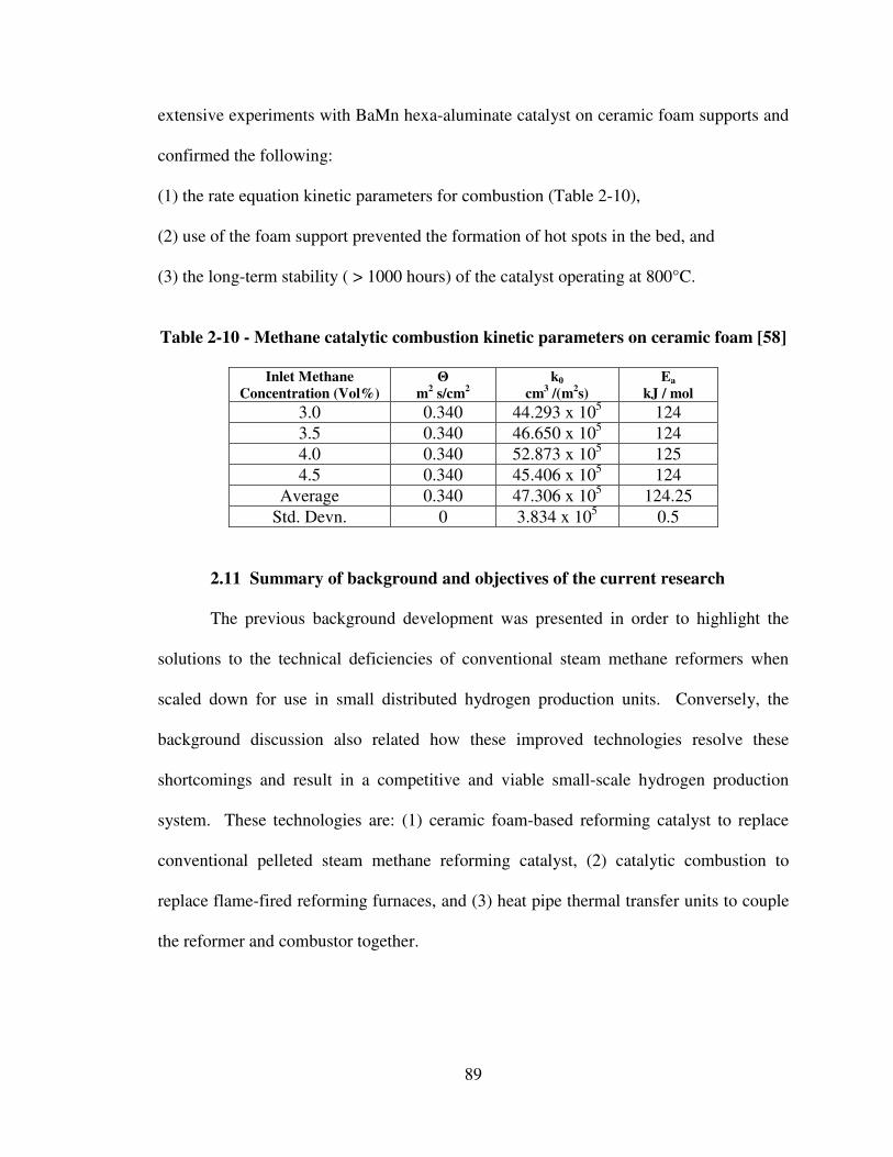
89
extensive experiments with BaMn hexa-aluminate catalyst on ceramic foam supports and
confirmed the following:
(1) the rate equation kinetic parameters for combustion (Table 2-10),
(2) use of the foam support prevented the formation of hot spots in the bed, and
(3) the long-term stability ( > 1000 hours) of the catalyst operating at 800°C.
Table 2-10 - Methane catalytic combustion kinetic parameters on ceramic foam [58]
Inlet Methane
Concentration (Vol%)
Θ
m2 s/cm
2
k0
cm3 /(m
2s)
Ea
kJ / mol
3.0 0.340 44.293 x 10⁵
124
3.5 0.340 46.650 x 10⁵ 124
4.0 0.340 52.873 x 10⁵ 125
4.5 0.340 45.406 x 10⁵ 124
Average 0.340 47.306 x 10⁵ 124.25
Std. Devn. 0 3.834 x 10⁵ 0.5
2.11 Summary of background and objectives of the current research
The previous background development was presented in order to highlight the
solutions to the technical deficiencies of conventional steam methane reformers when
scaled down for use in small distributed hydrogen production units. Conversely, the
background discussion also related how these improved technologies resolve these
shortcomings and result in a competitive and viable small-scale hydrogen production
system. These technologies are: (1) ceramic foam-based reforming catalyst to replace
conventional pelleted steam methane reforming catalyst, (2) catalytic combustion to
replace flame-fired reforming furnaces, and (3) heat pipe thermal transfer units to couple
the reformer and combustor together.

90
The objectives of this research project were to evaluate and demonstrate the
advantages of ceramic foam catalyst bed heat pipe reactors over conventional hydrogen
production technology for a 500 kg/day compact hydrogen production unit by:
(1) updating the prior 2-dimensional catalytic pellet bed reactor model to reflect the mass
transfer, heat transfer, and pressure drop improvements provided by ceramic foam
catalyst supports,
(2) finding the best configuration and arrangement of both the reformer and combustor
reactors with the model, and matching their performance when coupled with a heat
pipe,
(3) validating the updated computer model with experimental heat transfer and reaction
data, and upgrading the model as needed,
(4) further checking the model with parametric evaluations to verify that the model
predictions behaved as expected when key operating parameters, including feed rate,
inlet temperature, wall temperature, space velocity, and kinetic pre-exponential factor
were varied,
(5) utilizing the vetted model to size and specify the process equipment and supporting
facilities required for a 500 kg/day hydrogen production unit,
(6) completing an economic analysis on the new technology 500 kg/day hydrogen
production unit and comparing its delivered price of hydrogen to conventional
hydrogen production technology.

91
CHAPTER THREE
Reactor simulation models
3.1 Introduction
The research begins with an upgraded computer model for the compact integrated
Reformer/Heat Pipe/Combustor system, one stage at a time. Existing models, which
were used as a starting point were all written in the FORTRAN computer language,
requiring a FORTRAN compiler. To simplify the use of these models, and make them
more convenient for modern desktop computers, the original FORTRAN programs and
routines were translated and adapted into Microsoft’s Visual Basic for Applications
(VBA) language, which runs within Microsoft’s Office™ suite. As implemented, the
programs utilize a Microsoft Excel™ user interface for entering user data and parameters
and for displaying output directly into Excel™ tables and/or graphs. This allows
interactive adjustments of the reaction parameters directly by the user, by invoking
macros within Excel™ to run the program, without having to run any additional software.
To build these models within VBA, the steps undertaken were
(1) translate the historical 2-dimensional reformer FORTRAN model program into VBA.
(2) modify the working VBA model for the reformer into a model for the ceramic foam
catalytic heater.
3.2 Two-dimensional catalytic reactor basic equations
A starting assumption for the model is that mass diffusion along the axis is
negligible because the normal axial gas velocity is several orders of magnitude greater
than the axial diffusion velocity. No such simplification is available, however, for axial
thermal diffusion. Because of the high endothermic and exothermic nature of the

92
reforming and combustion reactions, respectively, temperature gradients exist in both the
radial and axial directions. Therefore, accurate reactor modeling requires a 2-
dimensional pseudo homogeneous model. These studies were undertaken to use the 2-
dimensional model, together with experimental results, to extract parameters for heat
transfer correlations and to use the model for reactor design purposes.
Physically, the heat pipe reactor was configured as a concentric annulus around a
central cylindrical heat pipe. This was the original design first experimental test. With a
change in boundary conditions, it can also be configured as a cylindrical catalyst bed
inside of an annular heat pipe, which is a more convenient and efficient design used in
this study. These are shown in Figures 3-1 and 3-2, respectively.
Ignoring axial dispersion, the steady-state computer model calculates the mass
balance and energy balance for each differential element of the catalyst bed in 2-
dimensions using radial coordinates (r – radial, and z – axial). The differential element is
a ring-shaped portion of the catalyst bed as shown in Figure 3-3.
Figure 3-1 - Annular heat pipe reactor surrounding an internal heat pipe.
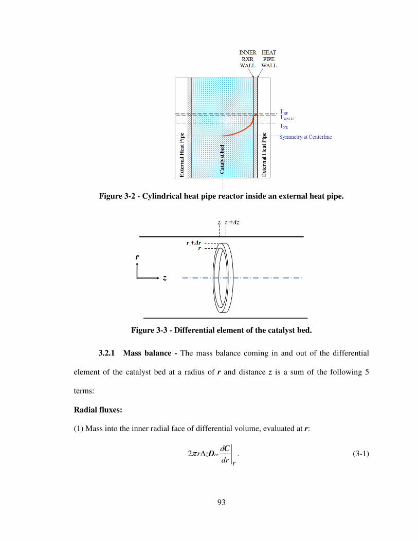
93
Figure 3-2 - Cylindrical heat pipe reactor inside an external heat pipe.
Figure 3-3 - Differential element of the catalyst bed.
3.2.1 Mass balance - The mass balance coming in and out of the differential
element of the catalyst bed at a radius of r and distance z is a sum of the following 5
terms:
Radial fluxes:
(1) Mass into the inner radial face of differential volume, evaluated at r:
2 erd
r zdr r
π ∆C
D . (3-1)

94
(2) Mass leaving outer radial face of differential volume, evaluated at r+∆r:
2 ( ) erd
r r zdr r r
π + ∆ ∆
+ ∆
CD . (3-2)
Axial fluxes:
(3) Mass entering left hand axial face of differential volume, evaluated at z:
2 r r vz
π ∆ C . (3-3)
(4) Mass leaving right hand axial face of differential volume, evaluated at z+∆z:
2 r r vz z
π ∆+ ∆
C . (3-4)
Reaction within the differential element
(5) Reaction within the differential volume:
2 r r zRateπ ∆ ∆ . (3-5)
Summing all 5 terms results in the steady mass balance equation for the differential
element;
0 2 2 ( )er erd d
r z r r zdr drr r r
π π= ∆ − + ∆ ∆ +
+ ∆
C CD D
2 2 2r r v r r v r r zRatez z z
π π π∆ − ∆ − ∆ ∆+ ∆
C C . (3-6)
Rearranging this equation and allowing ∆r →0 and ∆z →0 , the differential form of the
mass balance equation is obtained:
2
2
1er Rater
z v r r vr
∂ ∂∂= + +
∂ ∂∂
C D C C. (3-7)
Simplify the equation by introducing the definition of the Peclet number, namely;
p
rea
vPe =
D
D, or
ea p
rv Pe=
D D, (3-8)
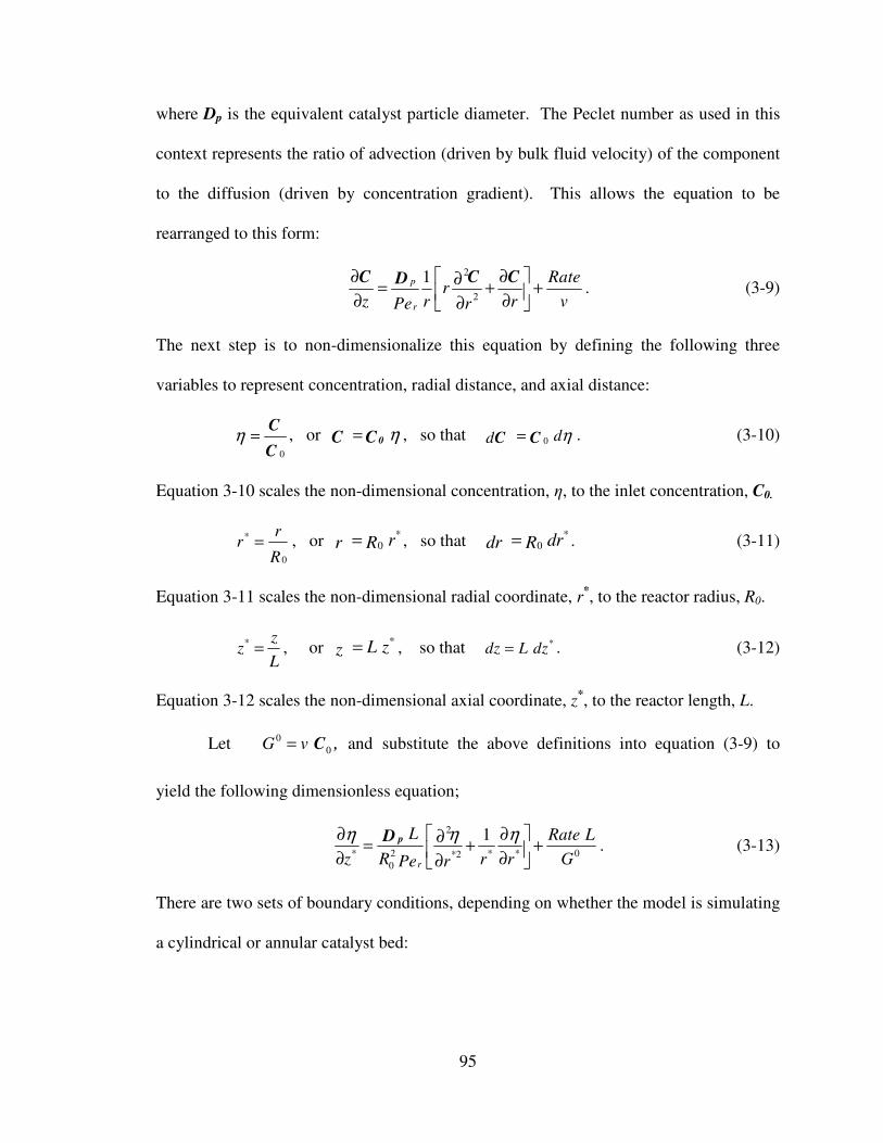
95
where Dp is the equivalent catalyst particle diameter. The Peclet number as used in this
context represents the ratio of advection (driven by bulk fluid velocity) of the component
to the diffusion (driven by concentration gradient). This allows the equation to be
rearranged to this form:
2
2
1p
r
Rater
z r r vPe r
∂ ∂∂= + +
∂ ∂∂
C C CD. (3-9)
The next step is to non-dimensionalize this equation by defining the following three
variables to represent concentration, radial distance, and axial distance:
0
η =C
C, or η= 0C C , so that 0 dd η=C C . (3-10)
Equation 3-10 scales the non-dimensional concentration, η, to the inlet concentration, C0.
*
0
rr
R= , or
*0 rr R= , so that
*0 drdr R= . (3-11)
Equation 3-11 scales the non-dimensional radial coordinate, r*, to the reactor radius, R0.
* zz
L= , or
* L zz = , so that * dz L dz= . (3-12)
Equation 3-12 scales the non-dimensional axial coordinate, z*, to the reactor length, L.
Let 0
0 G v= C , and substitute the above definitions into equation (3-9) to
yield the following dimensionless equation;
2
* 2 * * 0*20
1
r
L Rate L
z R r r GPe r
η η η ∂ ∂∂= + +
∂ ∂∂
pD. (3-13)
There are two sets of boundary conditions, depending on whether the model is simulating
a cylindrical or annular catalyst bed:

96
Boundary conditions for a cylindrical catalyst bed
*
= 0z
η∂
∂
at * = 0r , (3-14)
where * = 0r is the center axis of symmetry of the catalyst bed. This is the symmetry
boundary condition at the center of the bed.
*
= 0z
η∂
∂
at * = 1r , (3-15)
where * = 1r is the outer boundary of the cylindrical catalyst bed. There is no mass flux
at the outer edge of the bed in contact with the reactor wall, which is next to the heat
pipe.
Boundary conditions for an annular catalyst bed
*
= 0z
η∂
∂
at *
0 = r r R , (3-16)
where *
0 = r r R is the non-dimensional inner diameter of the annular catalyst bed
which is in contact with the reactor wall, next to which is the heat pipe. There is no mass
flux across this boundary,
*
= 0z
η∂
∂
at * = 1r , (3-17)
where * = 1r is the outer diameter of the annular catalyst bed, against the outer reactor
wall. There is no mass flux across this boundary.
3.2.2 Energy Balance - Similarly, an energy balance around the same
differential volume yields the following dimensional equation:
1 1
c
Reff
z p z p
Rate HT Trk
z v c r r r vρ ρ
∆∂ ∂ ∂ = −
∂ ∂ ∂ . (3-18)

97
For the energy balance, the non-dimensional variables are;
* a
HP a
T TT
T T
−=
−
, so that ( )*
HP adT T T dT= − . (3-19)
Equation 3-19 scales the non-dimensional temperature, T*, to the difference between the
heat pipe temperature, THP, and the system ambient temperature, Ta,
*
0
rr
R= , or
*0 rr R= , so that
*0 drdr R= . (3-20)
As before, equation 3-20 scales the non-dimensional radial coordinate, r*, to the reactor
radius, R0, and
* zz
L= , or
* L zz = , so that * dz L dz= , (3-21)
where equation 3-21 scales the non-dimensional axial coordinate, z*, to the reactor length,
L.
Let TG vρ= , and substitute the non-dimensional variables into the energy
balance equation to yield;
( )
* **
* 2 * * *
0
1 1R
eff
T p T p HP a
Rate H LT L Tr k
z G c R r r r G c T T
∆∂ ∂ ∂= −
∂ ∂ ∂ − . (3-22)
Expanding equation (3-22) leads to;
( )
* * 2 * *
* 2 * * *2 * *
0
1 effR
eff
T p T p HP a
Rate H LT L k T T T kk
z G c R r r r r r G c T T
∆∂ ∂ ∂ ∂ ∂= + + −
∂ ∂ ∂ ∂ ∂ − . (3-23)
Boundary conditions for a cylindrical catalyst bed:
(a) The symmetry condition at the center of a cylindrical bed is
*
* = 0
z
T∂
∂
at * = 0r , (3-24)
where * = 0r is the center axis of symmetry of the catalyst bed.

98
(b) The outer boundary condition of a cylindrical catalyst bed is
( )
( )
* 1HP a
HP a
T TT
T T
−
= =
−
at * = 1r , (3-25)
where r* = 1 is the outer edge of the bed. The outer edge of the catalytic bed is in closest
proximity to the heat pipe operating at 800°C, separated only by the reactor wall. It
should also be noted that internal non-dimensional temperatures at radial positions
between the two boundary conditions from 0 < r* < 1, may exceed 1, since the catalyst
bed temperatures may exceed that of the heat pipe.
Boundary conditions for an annular catalyst bed:
(a) The inner wall boundary condition for an annular catalyst bed is
( )
( )
* 1HP a
HP a
T TT
T T
−
= =
−
at *
0 = r r R , (3-25)
where *
0 = r r R is the non-dimensional inner diameter of the annular catalyst bed which
is in contact with the reactor wall, next to which is the heat pipe. The inner edge of the
annular catalytic bed is in closest proximity to the heat pipe operating at 800°C, separated
only by the reactor wall.
(b) The external boundary condition for the annular catalyst bed is
( )
( )
* 0a a
HP a
T TT
T T
−
= =
−
at * = r ∞ , (3-27)
where * = r ∞ is the distance away from the reactor where ambient conditions prevail.
3.2.3 Discretization of the mass and energy balances - With the mass and
energy balance equations in their non-dimensional forms:
2
* 2 * * 0*20
1 p
r
L Rate L
z R r r GPe r
η η η ∂ ∂∂= + +
∂ ∂∂
D, and (3-13)
99
( )
* * 2 * *
* 2 * * *2 * *
0
1 effR
eff
T p T p HP a
Rate H LT L k T T T kk
z G c R r r r r r G c T T
∆∂ ∂ ∂ ∂ ∂= + + −
∂ ∂ ∂ ∂ ∂ − , (3-23)
it is now possible to discretize them in order to allow them to be coded into the computer
simulation. The partial derivatives can be replaced by these approximations: For the
partial derivatives of non-dimensional concentration, η , with respect to r*, The finite
difference equation for forward differences yield the following two equations;
( )
( )( 1, ) ( , ) *
* ** 0
limi j i j
r
O rr r
η ηη +
∆ →
−∂≅ + ∆
∂ ∆
, and (3-28)
( )
( )
2( 2, ) ( 1, ) ( , ) *
*2 *2* 0
2lim
i j i j i j
r
O rr r
η η ηη + +
∆ →
− +∂≅ + ∆
∂ ∆
, (3-29)
where O(∆r*) denotes the error between the true derivative (left hand side) and the finite
difference approximation (right hand side). In this case, O(∆r*) denotes an error of the
order of ∆r*. The forward finite difference equation for the first derivative uses two
calculated function values at points ηi, and at ηi+1, while the forward finite difference
equation for the second derivative uses three points, at ηi, ηi+1, and at ηi+2.
It is possible to reduce the inherent error of these finite difference equations by
changing from a forward difference equation to a centered difference equation. In the
case of the first derivative, the finite difference equation changes to
( )
( )( 1, ) ( 1, ) *2
* ** 0
lim2
i j i j
r
O rr r
η ηη + −
∆ →
−∂≅ + ∆
∂ ∆
, and (3-30)
in which the first derivative centered finite difference equation is now evaluated at ηi-1
and ηi+1, instead of ηi and ηi+1, and over two increments of ∆r*, hence the factor of 2 in
the denominator. The benefit is that now, the error term is of the order of ∆r*2
instead of
∆r*, which is a significant improvement. In the same manner, the second derivative
100
forward finite difference equation can be converted to a centered finite difference
equation, to
( )
( )
2( 1, ) ( , ) ( 1, ) *2
*2 *2* 0
2lim
i j i j i j
r
O rr r
η η ηη + −
∆ →
− +∂≅ + ∆
∂ ∆
, (3-31)
in which the second derivative centered finite difference equation is now evaluated at
ηi-1, ηi, and ηi+1, instead of ηi, ηi+1 and ηi+2. As in the case of the first derivative centered
finite difference equation, the error term is now of the order of ∆r*2
, instead of ∆r*.
A similar derivation of the centered finite difference equations for the partial
derivatives of non-dimensional temperature, T* , with respect to r
*, yields:
( )
( )
* **( 1, ) ( 1, ) *2
* ** 0
lim2
i j i j
r
T TTO r
r r
+ −
∆ →
−∂≅ + ∆
∂ ∆
, (3-32)
( )
( )
* * *2 *( 1, ) ( , ) ( 1, ) *2
*2 *2* 0
2lim
i j i j i j
r
T T TTO r
r r
+ −
∆ →
− +∂≅ + ∆
∂ ∆
, and (3-33)
( )
( )( 1, ) ( 1, ) *2
* ** 0
lim2
i j i j
r
k kkO r
r r
+ −
∆ →
−∂≅ + ∆
∂ ∆
. (3-34)
When these finite difference equations are substituted into the mass balance and
energy balance equations, we obtain the final form of the non-dimensional equations
which are suitable for use in the computer simulation:
Mass balance:
( ) ( )( )
( 1, ) ( , ) ( 1, ) ( 1, ) ( 1, ) *2
* 2 *2 * * 0
0
2 1 ,
2
i j i j i j i j i jp
r
L Rate LO r
z R r r r GPe
η η η η ηη + − + −
− + −∂ = + + + ∆
∂ ∆ ∆
D
(3-35)
Energy Balance:
( ) ( )* * * * **
( 1, ) ( 1, ) ( 1, ) ( , ) ( 1, )
* 2 * * *2
0
21
2
eff i j i j i j i j i j
T p
T T T T TT Lk
z G c R r r r
+ − + −
− − +∂= + +
∂ ∆ ∆

101
( ) ( )
( )( )
* *
( 1, ) ( 1, ) ( 1, ) ( 1, ) *2
* *
1
2 2
i j i j i j i j R
eff T p HP a
T T k k Rate H LO r
k r r G c T T
+ − + −
− − ∆ − + ∆
∆ ∆ −
. (3-36)
The boundary conditions are as stated above in equations 3-14 through 3-17 for
the mass balance, and equations 3-24 through 3-27 for the energy balance.
3.2.4 Step sizes for the numerical integration - The direction of integration is
along the z axis, using the Euler method for each dimensionless variable as follows,
where hz is the step size increment along the z axis;
*
*
* * *1
z
z z zh
z
η
η η+
∂
= +
∂
, (3-37)
*
* *
*
*
*
**1
z
z z z
TT T h
z+
∂
= +
∂
. (3-38)
3.2.5 Parameter inputs – The user inputs the following parameters to evaluate
their effects on the reactor performance:
(1) Reactor dimensions – The diameter and length of the reactor are needed to quantify
the volume of the catalyst bed. In the case of the cylindrical reactor, only the diameter
(DREA) and length (LENGTH) are required. In the case of the annular reactor with an
internal heat pipe, the heat pipe diameter (DHP) and reactor wall thickness (XWALL) are
additional parameters which are required so that the volume of the internal heat pipe is
properly excluded from the volume of the annular catalyst bed .
(2) Catalyst bed parameters – These are required to specify the catalytic activity and heat
transfer characteristics of the catalyst bed. The catalyst activation energy (AE), pre-
exponential factor (RK0), and pre-exponential factor coefficient (FK) are used in
calculating the kinetic behavior of the bed. The physical properties of the bed, include

102
the void fraction (E) and the catalyst effective particle diameter (DPH). The effective
heat transfer coefficient (KEFF) is an empirical relation based on experimental data, and
can easily be entered into the VBA code.
(3) Feed streams – The reformer model methane (CH4) and steam (STEAM) feed rates
are in units of standard liters per minute (SLPM). The combustor model replaces the
steam flow with an air flow (AIR).
(4) Process conditions – The operating pressure of the system (PRESS) is in units of atm.
All of the starting temperatures are in ºC, including the inlet gas (TIN), heat pipe (THP),
exterior surface of the insulation (TINSUL), and the ambient (TINF) temperatures.
(5) Fluid properties –Fluid properties can be modified by the user, if needed. The
properties which can be changed within the Excel™ interface include molecular weight
(MW) and heat capacity equation coefficients (CPA through CPD). Other gas properties
that are functions of temperature which can be changed within the VBA code include
enthalpy of formation, viscosity, and thermal conductivity.
3.3 Heat transfer modeling: thermal resistances and conductivities
The basis for computational modeling of the thermal resistances and
conductivities in the heat pipe reactor was initially formulated for a packed bed of pellets
[51]. This foundation was then applied to ceramic foam substrates, when the appropriate
changes to the bed properties were modified in the model.
Earlier researchers (Kulkarni & Doraiawamy) found that the effective thermal
conductivity was best modeled in a composite parallel-series configuration proposed by
Argo and Smith [65]. This assumes radial conduction, radiation, and convection to be

103
parallel in the fluid (gas) phase, but in series in the solids (catalytic bed) phase. Modeled
this way, the effective thermal conductivity takes the form of
keff = δ( kconduction + kradiation + kconvection ) + (1-δ) kseries , << W · cm-1
· K-1
>> , (3-39)
where δ is the void fraction of the bed, in units of (cm3void / cm
3bed), kconduction, kradiation,
kconvection, and kseries are the conductive, radiative, convective, and series thermal
conductivities, respectively of the fluid and the catalyst bed.
The conductive thermal conductivity of the fluid, kc, is calculated in the program
from km, the thermal conductivity of the gas mixture. km is calculated by multiplying
each gaseous component’s thermal conductivity by its respective mole fraction, and
summing over all the components, and has the units of Watts×cm-1
׺K-1
,
1
n
conduction mixture i i
i
k k y k=
= =∑ << W·cm-1·K
-1 >>. (3-40)
The radiative contribution of thermal conductivity, kradiation , is defined as
( )
11 32.29 10
2
sradiation p
s
k Tε
ε
−
= × ×
−
D , << W·cm-1·K
-1 >>, (3-41)
in which Dp is the equivalent diameter of the particle, in cm, sε is the emissivity of the
catalyst, and T is the temperature, in ºK, and also has the units of Watts×cm-1
׺K-1
. The
convective contribution to thermal conductivity, kcv, is defined as
,
p
convection T p mixture
r
k G cPeδ
=
D, << W·cm
-1·K
-1 >> , (3-42)
in which GT is the total molar flux, in units of gmol·cm-2
·sec-1
, cp,mixture is the heat capacity
of the gas mixture, with units of J·gmol-1
·K-1
, Dp is the equivalent diameter of the catalyst
particle, in cm, δ is the void fraction of the bed, and Per is the radial Peclet number.
Kconvection also has units of Watts×cm-1
׺K-1
.

104
With respect to the solid phase, the thermal conductivity, kseries, is calculated by
2
solid s p
series
s solid p
h kk
k h=
+
D
D << W·cm
-1·K
-1 >> , (3-43)
where ks is the thermal conductivity of the solid in W·cm-1
·K-1
, Dp is the equivalent
particle diameter in cm, and the heat transfer coefficient for the solid phase, hsolid , is
solid conduction convection radiationh h h h= + + << W·cm
-2·K
-1 >> . (3-44)
The conduction heat transfer coefficient, hconduction , is defined as
( )2 s solid p
conduction p
p s
k hh k
k
+
=
D
D << W·cm
-2·K
-1 >> , (3-45)
where kp is the thermal conductivity of the pellet, which has been determined as
0.7453.52
10
s
p
k
kδ
− +
= << W·cm-1·K
-1 >> . (3-46)
The convection heat transfer coefficient, hconvection, is defined for two ranges of Reynolds
numbers, Rp, to be
0.51
,
2 31.95
T p mixture
convection
G c Reh
Pr
−
= , for REp < 350, << W·cm-2·K
-1 >>, or (3-47)
0.41
,
2 31.06
T p mixture
convection
G c Reh
Pr
−
= , for REp > 350, << W·cm-2·K
-1 >>. (3-48)
in which the Prandtl number, Pr, and Reynolds number, Rep, are defined as
,p mixture mixture
mixture
cPr
k
µ
= , and (3-49)
T p
p
mixture
GRe
µ
=
D. (3-50)
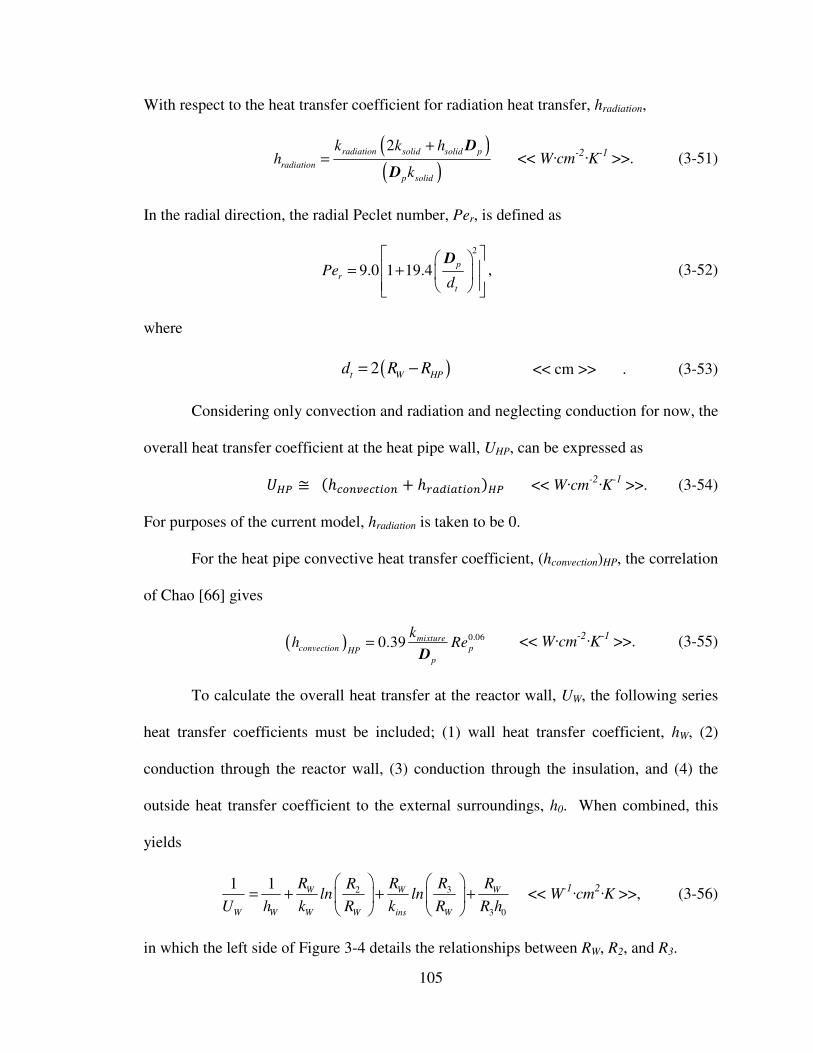
105
With respect to the heat transfer coefficient for radiation heat transfer, hradiation,
( )
( )
2radiation solid solid p
radiation
p solid
k k hh
k
+
=
D
D << W·cm
-2·K
-1 >>. (3-51)
In the radial direction, the radial Peclet number, Per, is defined as
2
9.0 1 19.4p
r
t
Ped
= +
D, (3-52)
where
( )2t W HP
d R R= − << cm >> . (3-53)
Considering only convection and radiation and neglecting conduction for now, the
overall heat transfer coefficient at the heat pipe wall, UHP, can be expressed as
!" ≅ �ℎ%&'()%*+&' + ℎ,-.+-*+&'�!" << W·cm-2·K
-1 >>. (3-54)
For purposes of the current model, hradiation is taken to be 0.
For the heat pipe convective heat transfer coefficient, (hconvection)HP, the correlation
of Chao [66] gives
( )0.06
0.39 mixtureconvection pHP
p
kh Re=
D << W·cm
-2·K
-1 >>. (3-55)
To calculate the overall heat transfer at the reactor wall, UW, the following series
heat transfer coefficients must be included; (1) wall heat transfer coefficient, hW, (2)
conduction through the reactor wall, (3) conduction through the insulation, and (4) the
outside heat transfer coefficient to the external surroundings, h0. When combined, this
yields
32
3 0
1 1 W W W
W W W W ins W
R R R RRln ln
U h k R k R R h
= + + +
<< W
-1·cm
2·K >>, (3-56)
in which the left side of Figure 3-4 details the relationships between RW, R2, and R3.

106
Figure 3-4 - Axial flow cylindrical ceramic foam reactor radii for heat transfer
coefficients.
Additionally, the right side for Figure 3-4 shows the relationship between Ta, Tins, TW,
TNR, T0, and THP. Note that TW is the temperature of the reactor inner wall, while TNR is
the temperature of the outermost radial increment of the catalyst bed. They are not the
same, and these two temperatures would have been used to calculate the radiation heat
transfer coefficient at the reactor wall, (hradiation)W, if it was used, represented by
( )
4 4
1 11
NR Wradiation W
NR W
W solid
T Th
T T
σ
ε ε
−=
− + −
<< W·cm-2·K
-1 >>, (3-57)
where Wε is the emissivity for the reactor wall, and solid
ε is the emissivity of the catalyst
solid. The convective heat transfer coefficient at the wall, (hconvection)W, is given by
( )0.06
0.39 mixtureconvection pW
p
kh Re=
D << W·cm
-2·K
-1 >>. (3-58)
For the outer surface of the insulation, the outside heat transfer coefficient, h0, is
( )0 radiation nat convinsh h h= + , << W·cm
-2·K
-1 >>, (3-59)
in which

107
( )
4 4
0.9 ins aradiation ins
ins a
T Th
T Tσ
−=
− << W·cm
-2·K
-1 >>, (3-60)
and the heat transfer coefficient for natural convection, per McCabe and Smith [67] is
( ) conv
nfilm
nat fillm
kh b Gr Pr
L= × << W·cm
-2·K
-1 >>, (3-61)
where b and n depend on the product of the Grashof and Prandtl numbers, /0 × �0, as
follows;
if 101 < /0 × Pr < 104, 6ℎ78 9 = 0.59 ;8< 8 = 0.25, and (3-62)
if 104 < /0 × Pr < 10>?, 6ℎ78 9 = 0.13 ;8< 8 = 0.333. (3-63)
The intrinsic reaction rate, R, was determined experimentally in a laboratory
reaction system. To calculate the effectiveness factor, η, a generalized Thiele modulus,
ϕ, was calculated per the following:
( )
( )
4
4
4
4
0.5
0.52
SCH
eq
CH
S C
CH pp
p CH
effx C
R CVR dC
S
ρ
φ ρ
−
=
∫
D , (3-64)
which in turn gives ( )
2
3 3 1
3
cothφ φ
η
φ
−
= . (3-65)
The experimentally-determined intrinsic rate equation for 20% Ni/α-Al2O3
reforming catalyst is expressed as
4
53,326
28.82 10 RT
CHRate e p
−
− = × << Mol·sec
-1·g cat
-1 >>. (3-66)
3.4 Excel™ model
The computer model has two means of modifying input information to evaluate
the effect they have on predicted reactor operation. First is an Excel™ interface, which is

108
used to adjust the more commonly evaluated input parameters like feed rate, inlet and
operating temperatures, and reactor dimensions. The Excel™ interface is also where the
output of the model is displayed, including graphs, data tables, and calculation results.
The second means of modifying input to the model is the VBA code itself, which can be
modified to make more significant changes in the model to reflect updates to the less
commonly-adjusted parameters, like physical properties, heat transfer correlations, or
boundary conditions.
3.4.1 Excel™ interface - The model, which is programmed in VBA, uses an
Excel™ user interface with which to enter program input parameters under evaluation.
The Excel™ interface is set up for the most commonly adjusted reactor parameters,
including (1) reactor dimensions, (2) operating temperatures, (3) feed rates, and (4)
certain catalyst parameters. It also has a limited set of fluid property data that can be
changed within Excel™ that includes molecular weight and heat capacity. An example
of the input sheet for the reactor parameters within Excel™ is displayed in Figure 3-5,
while the input sheet for physical property parameters is shown in Figure 3-6.
After the model program executes, the Excel™ interface is also where the output
information is displayed as tables of results. As with any other Excel™ spreadsheet,
these tables are transferred directly into pre-formatted graphs for display within Excel™,
or exported for further analysis.
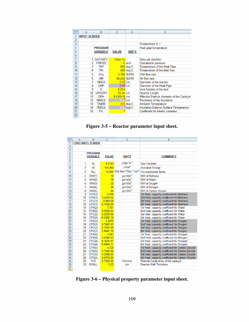
109
Figure 3-5 – Reactor parameter input sheet.
Figure 3-6 – Physical property parameter input sheet.
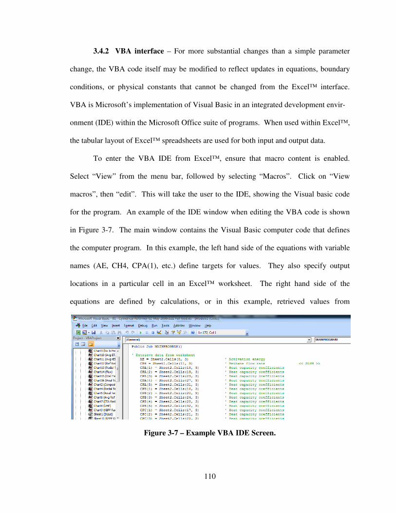
110
3.4.2 VBA interface – For more substantial changes than a simple parameter
change, the VBA code itself may be modified to reflect updates in equations, boundary
conditions, or physical constants that cannot be changed from the Excel™ interface.
VBA is Microsoft’s implementation of Visual Basic in an integrated development envir-
onment (IDE) within the Microsoft Office suite of programs. When used within Excel™,
the tabular layout of Excel™ spreadsheets are used for both input and output data.
To enter the VBA IDE from Excel™, ensure that macro content is enabled.
Select “View” from the menu bar, followed by selecting “Macros”. Click on “View
macros”, then “edit”. This will take the user to the IDE, showing the Visual basic code
for the program. An example of the IDE window when editing the VBA code is shown
in Figure 3-7. The main window contains the Visual Basic computer code that defines
the computer program. In this example, the left hand side of the equations with variable
names (AE, CH4, CPA(1), etc.) define targets for values. They also specify output
locations in a particular cell in an Excel™ worksheet. The right hand side of the
equations are defined by calculations, or in this example, retrieved values from
Figure 3-7 – Example VBA IDE Screen.

111
specific cells within an Excel™ worksheet. Once in the main part of the program, the
user may modify whatever part of the code requires updating for the particular evaluation
at hand. The entire listings for the VBA code for both the reformer and combustor
models are included in Appendix 1 and 2, respectively.
3.5 Determining heat transfer correlations of 30-PPI αααα-Al2O3 ceramic foam
Experimental data for 30-PPI α-Al2O3 ceramic foams was presented by Peng, who
studied the properties of ceramic foam substrates with respect to pressure drop and heat
and mass transfer [53, 57]. Peng tested the heat transfer properties of a ceramic foam
reactor at various air flow rates and temperatures, without reaction. The test reactor
consisted of a 5.08 cm (2 inch) diameter by 15.24 cm (6 inch) long ceramic foam bed, in
which multiple thermocouples were installed to measure the bed temperatures both
radially from the center of symmetry, and longitudinally, along its length. In the radial
direction, the temperature was measured at dimensionless radii (r / R) of 0, 0.35, 0.65,
0.85, and 1.00. In the longitudinal direction, the temperature was measured every 2.54
cm at 0, 2.54, 5.08, 7.62, 10.16, 12.70, and 15.24 cm. These thermocouple measuring
points are shown schematically in Figure 3-8.
This reactor was tested under 17 different sets of conditions in which the air flow
rate, inlet temperature, and external wall temperature were varied. Since an external
heater was used, the wall temperature was not isothermal in the longitudinal direction.
Therefore, the wall temperature profile along the longitudinal axis was represented as a
third-degree polynomial function of the axial distance.
These experiments yielded 17 sets of radial and axial temperature profiles that
Peng used to determine parameters for the correlation equations:

112
Nusselt number based on Sv 3
Reeff p
Sg
kT bαε
λ
= +D
, (3-67)
wall heat transfer coefficient Re d
w gS
cα λ= , (3-68)
Figure 3-8 - Schematic of thermocouple locations in the laboratory ceramic bed.
where a, b, c, d are undetermined constants,
Dp is the foam pore diameter, or equivalent particle diameter,
ε is the foam porosity or packed bed void fraction,
keff is the effective heat transfer coefficient,
λg is the thermal conductivity of the gas,
Res is the Reynolds number based on external surface area per volume of solid,
Sv is external surface area per volume of solid = 4
(1 )p
ε
ε−D.
Using a non-linear curve fitting program for the complete set of data, Peng
determined the following heat transfer equations for the 2-D model:
11 3
2.178 10 42.2 Reeff
Sg
kT
λ
−
= × + , and (3-69)
113
2 0.48
v6.92 10 S Rew
Sg
α
λ
−
= × . (3-70)
These equations were used in subsequent reactor simulations of exothermic and
endothermic processes [59]. It was found that, although the bed conductivity equation
gave reasonable predictions for enhanced radial heat transfer, the wall coefficient was too
low so that unrealistic heat transfer at the wall was realized. Accordingly, it was decided
to re-examine Peng’s data in order to achieve a more accurate wall coefficient.
3.6 Validation of the computer model, heat transfer only
This test was performed on the original Peng data without any combustion or
reforming reactions present, to assess the adequacy of both the convective and conductive
heat transfer correlations. It should also be noted, that for these computations, the
computer simulation also used Peng’s third-degree polynomials representing reactor wall
temperature profiles.
To demonstrate the inadequacies of the wall coefficient, the radial temperature
profiles generated by the computer model were compared to the lab data from Peng [57].
Figure 3-9 is an example of this early comparison, in which the dashed lines represent the
computer model predictions, and the symbols represent the lab data. On the right of
Figure 3-9 are the conditions at the wall of the reactor. At L = 0.20 (the blue trace on
Figure 3-9), the computer predicts that the temperature at the outermost edge of the
catalyst bed, just inside the wall, is 280ºC. However, the lab-measured temperature at the
wall under the same conditions is 352ºC. The computer model is predicting a thermal
resistance at the wall that results is a temperature difference of 72ºC between the outside
edge of the catalyst bed and the wall. That temperature difference is represented by the
vertical section of the blue dashed line at L = 0.20 on Figure 3-9. The same problem

114
exists for the other data on Figure 3-9 at L = 0.40, 0.60, and 0.80. Clearly, this
discrepancy made the computer model significantly understate the ability of the heat pipe
reactor to provide heat to the heat pipe when compared to actual laboratory data.
Figure 3-9 – Radial temperature profiles – model versus Peng data set 3 [57].
3.6.1 Model upgrades - To resolve this discrepancy at the wall, the heat transfer
coefficient calculation module in the computer model was thoroughly examined to
evaluate what factor was causing the model to create such a high thermal resistance at the
wall. The key heat transfer parameters at the wall are (1) UHP, the heat pipe overall heat
transfer coefficient, (2) KEFF, the effective heat transfer coefficient in the bed, and (3),
HCVHP, the heat pipe convective heat pipe heat transfer coefficient. Using dimensional
analysis to ensure that the proper engineering units (mass, distance, area, temperature)
were conserved, together with appropriate scaling factors (DR, DZ, DREA, L), these
three parameters were tested in multiple combinations and permutations to evaluate how
to adjust the computer model better fit the lab results of Peng. Several examples of the
tested forms of the parameters are shown in Table 3-1.

115
Table 3-1 – Model parameter testing to resolve high thermal resistance at the wall
Parameter Original form Tested form(s)
UHP (Heat pipe overall heat
transfer coefficient) UHP = 1# / (1# / HHP + HC)
UHP = KEFF * DR / (PI *
DREA * DZ)
UHP = KEFF * DR / (PI *
DHP * DZ)
UHP = KEFF / DR
KEFF (Effective thermal heat
transfer coefficient)
KEFF = 2.178×10⁻¹¹
×T3 +
7.262 × REP × TCM
KEFF / x, x = 2 to 16
KEFF * y, y = 0.5 to 2.0
HCVHP (Heat pipe convective
heat transfer coefficient)
HCVHP = 9.338 × REP0.48
×
TCM × 160
HCVHP / z, z = 10 to 160
HCVHP = KEFF / DR
A significant improvement in the model fit was discovered when (1) HCVHP (the
heat pipe convective heat transfer coefficient) is replaced with KEFF/DR, and (2) KEFF
is modified with a multiplicative factor of 0.724. This allows equation 3-70 to be
replaced by equation 3-71. At steady state flow conditions, the expression for αw
becomes:
eff
wk
drα = . (3-71)
This equation is also consistent with the concept that, unlike a packed bed of pellets, the
ceramic foam structure is maintained all the way to the wall, i.e. porosity at the wall is the
same as in the bed.
While these changes were developed while studying data set 17 of Peng’s data,
improvement was seen over all of the lab data. For comparison, Figure 3-10 is an
updated result from the same dataset used in Figure 3-9. The improvement in the
temperature profiles at the wall is significantly better, as the predicted wall temperatures
come very close to the actual measured wall temperatures.
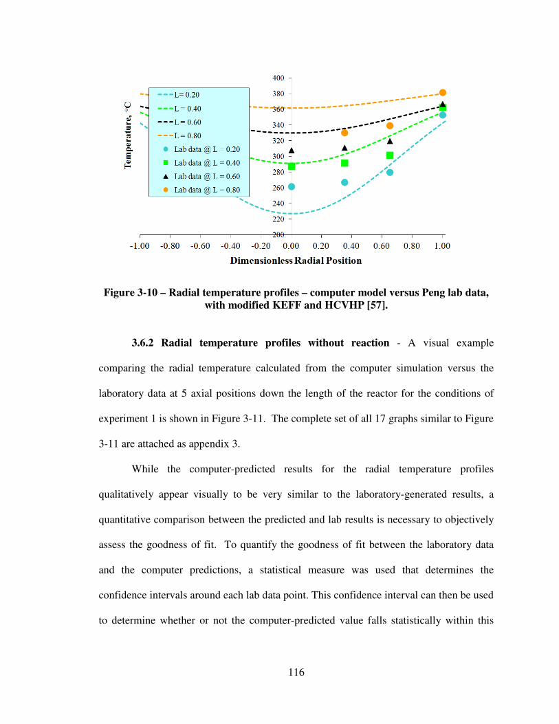
116
Figure 3-10 – Radial temperature profiles – computer model versus Peng lab data,
with modified KEFF and HCVHP [57].
3.6.2 Radial temperature profiles without reaction - A visual example
comparing the radial temperature calculated from the computer simulation versus the
laboratory data at 5 axial positions down the length of the reactor for the conditions of
experiment 1 is shown in Figure 3-11. The complete set of all 17 graphs similar to Figure
3-11 are attached as appendix 3.
While the computer-predicted results for the radial temperature profiles
qualitatively appear visually to be very similar to the laboratory-generated results, a
quantitative comparison between the predicted and lab results is necessary to objectively
assess the goodness of fit. To quantify the goodness of fit between the laboratory data
and the computer predictions, a statistical measure was used that determines the
confidence intervals around each lab data point. This confidence interval can then be used
to determine whether or not the computer-predicted value falls statistically within this

117
Figure 3-11 - Computer simulation results versus lab test number 1.
range. If the computer model prediction falls within the confidence intervals, it can be
interpreted as being a statistically significant fit.
The steps to analyze each of the 17 laboratory runs against the computer model
were as follows:
(1) For each different axial distance along the length of the catalyst bed, perform a
separate comparison analysis. The dimensionless distances down the bed were taken at
z/L = 0.167, 0.333, 0.500, 0.667, 0.833 and 1.00. Each of the 17 laboratory runs will
then have a standalone spreadsheet with 6 separate pages at each axial distance (z/L)
down through the bed.
(2) Take all n replicate measurements at each laboratory data point to find the mean at
each data point, x̄ . For instance, in the case of run 1, the number of replicates of each
data point was 5, so that n = 5.
(3) With m data levels (a data level was taken at each step in the radial direction, where
the dimensionless radial distance r/R = 0, 0.35, 0.65, 0.85, 1.00. Therefore, m = 5, in the
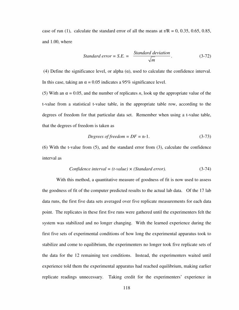
118
case of run (1), calculate the standard error of all the means at r/R = 0, 0.35, 0.65, 0.85,
and 1.00, where
Standard error = S.E. = Standard deviation
m. (3-72)
(4) Define the significance level, or alpha (α), used to calculate the confidence interval.
In this case, taking an α = 0.05 indicates a 95% significance level.
(5) With an α = 0.05, and the number of replicates n, look up the appropriate value of the
t-value from a statistical t-value table, in the appropriate table row, according to the
degrees of freedom for that particular data set. Remember when using a t-value table,
that the degrees of freedom is taken as
Degrees of freedom = DF = n-1. (3-73)
(6) With the t-value from (5), and the standard error from (3), calculate the confidence
interval as
Confidence interval = (t-value) × (Standard error). (3-74)
With this method, a quantitative measure of goodness of fit is now used to assess
the goodness of fit of the computer predicted results to the actual lab data. Of the 17 lab
data runs, the first five data sets averaged over five replicate measurements for each data
point. The replicates in these first five runs were gathered until the experimenters felt the
system was stabilized and no longer changing. With the learned experience during the
first five sets of experimental conditions of how long the experimental apparatus took to
stabilize and come to equilibrium, the experimenters no longer took five replicate sets of
the data for the 12 remaining test conditions. Instead, the experimenters waited until
experience told them the experimental apparatus had reached equilibrium, making earlier
replicate readings unnecessary. Taking credit for the experimenters’ experience in
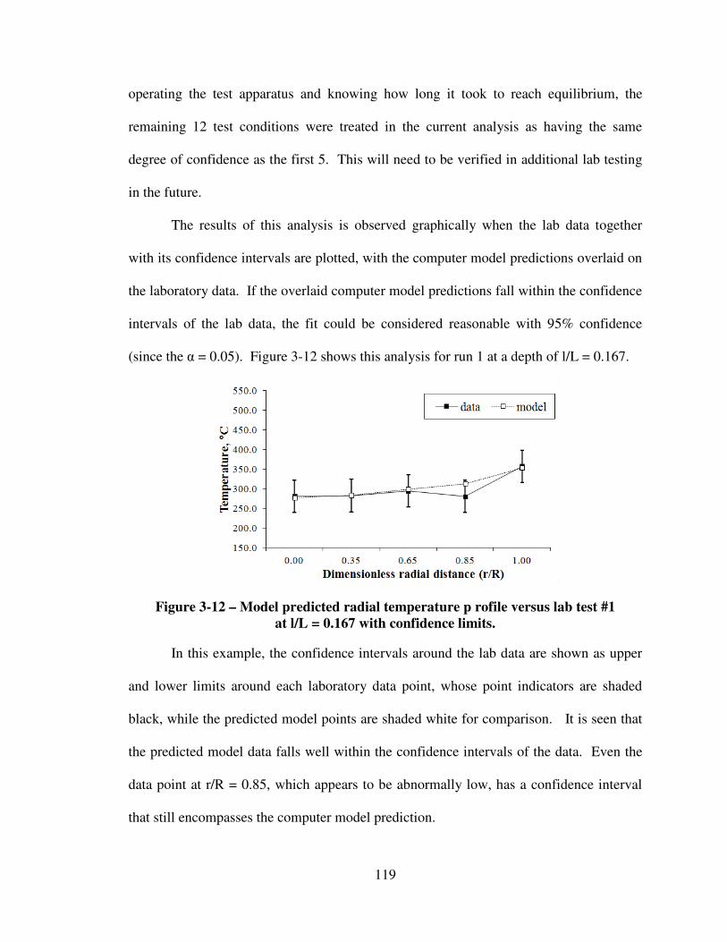
119
operating the test apparatus and knowing how long it took to reach equilibrium, the
remaining 12 test conditions were treated in the current analysis as having the same
degree of confidence as the first 5. This will need to be verified in additional lab testing
in the future.
The results of this analysis is observed graphically when the lab data together
with its confidence intervals are plotted, with the computer model predictions overlaid on
the laboratory data. If the overlaid computer model predictions fall within the confidence
intervals of the lab data, the fit could be considered reasonable with 95% confidence
(since the α = 0.05). Figure 3-12 shows this analysis for run 1 at a depth of l/L = 0.167.
Figure 3-12 – Model predicted radial temperature p rofile versus lab test #1
at l/L = 0.167 with confidence limits.
In this example, the confidence intervals around the lab data are shown as upper
and lower limits around each laboratory data point, whose point indicators are shaded
black, while the predicted model points are shaded white for comparison. It is seen that
the predicted model data falls well within the confidence intervals of the data. Even the
data point at r/R = 0.85, which appears to be abnormally low, has a confidence interval
that still encompasses the computer model prediction.
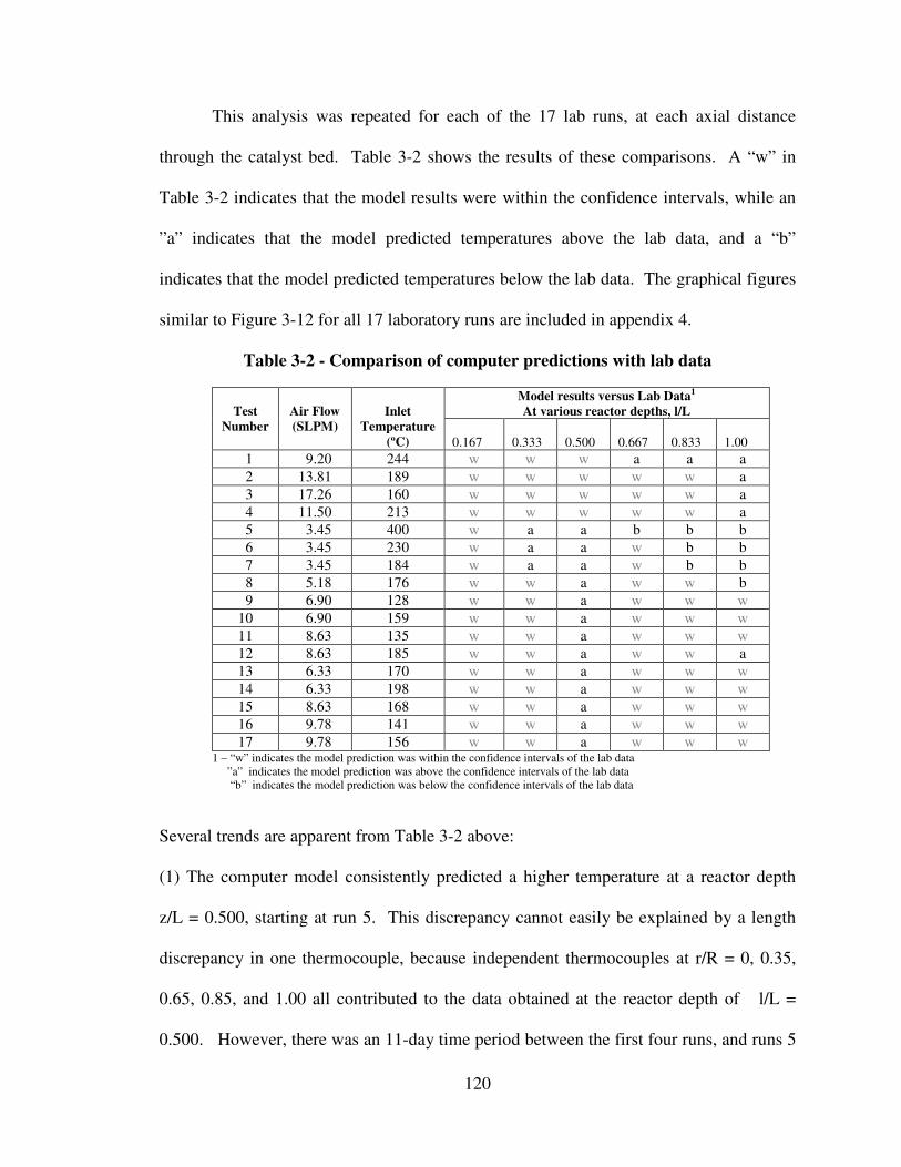
120
This analysis was repeated for each of the 17 lab runs, at each axial distance
through the catalyst bed. Table 3-2 shows the results of these comparisons. A “w” in
Table 3-2 indicates that the model results were within the confidence intervals, while an
”a” indicates that the model predicted temperatures above the lab data, and a “b”
indicates that the model predicted temperatures below the lab data. The graphical figures
similar to Figure 3-12 for all 17 laboratory runs are included in appendix 4.
Table 3-2 - Comparison of computer predictions with lab data
Test
Number
Air Flow
(SLPM)
Inlet
Temperature
(ºC)
Model results versus Lab Data1
At various reactor depths, l/L
0.167
0.333
0.500
0.667
0.833
1.00
1 9.20 244 w w w a a a
2 13.81 189 w w w w w a
3 17.26 160 w w w w w a
4 11.50 213 w w w w w a
5 3.45 400 w a a b b b
6 3.45 230 w a a w b b
7 3.45 184 w a a w b b
8 5.18 176 w w a w w b
9 6.90 128 w w a w w w
10 6.90 159 w w a w w w
11 8.63 135 w w a w w w
12 8.63 185 w w a w w a
13 6.33 170 w w a w w w
14 6.33 198 w w a w w w
15 8.63 168 w w a w w w
16 9.78 141 w w a w w w
17 9.78 156 w w a w w w 1 – “w” indicates the model prediction was within the confidence intervals of the lab data
”a” indicates the model prediction was above the confidence intervals of the lab data
“b” indicates the model prediction was below the confidence intervals of the lab data
Several trends are apparent from Table 3-2 above:
(1) The computer model consistently predicted a higher temperature at a reactor depth
z/L = 0.500, starting at run 5. This discrepancy cannot easily be explained by a length
discrepancy in one thermocouple, because independent thermocouples at r/R = 0, 0.35,
0.65, 0.85, and 1.00 all contributed to the data obtained at the reactor depth of l/L =
0.500. However, there was an 11-day time period between the first four runs, and runs 5

121
and later. Perhaps some improvements in the insulation between the laboratory reactor
and the heating system made the actual reactor less responsive to the externally applied
heat. The raw lab data certainly shows that for runs 1 through 4, the wall temperature
profile (largely determined by the external electrical heaters) along the length of the
reactor always increased from beginning to end. However, starting with run 5 and
continuing through the remaining runs, the wall temperature profile no longer increased
for the entire length of the reactor, but reached a peak just after the halfway point through
the reactor, then dropped to a lower value by the end of the reactor. The behavior
observed with a temperature lag in the actual lab data versus the computer prediction seen
at z/L = 0.500 is characteristic of an added thermal resistance which is unaccounted for in
the computer model. This should be verified in future experiments.
(2) For the low flow cases, runs 5, 6, and 7, the computer predictions were both above the
actual lab data in the first half of the reactor, at z/L ≤ 0.500, and then below the actual lab
data in the last half of the reactor, where z/L > 0.500. This is indicative of an added
thermal resistance which is unaccounted for in the computer model in two ways. First, in
the beginning half of the reactor, an added thermal resistance, which is not accounted for
in the model, will cause the actual lab data to lag behind, and drop below the computer
prediction, as runs 5, 6, and 7 when z/L ≤ 0.500 in Table 3-3 indicate. Second, the
thermal energy input from the wall heaters reached a peak along the length of the reactor
just after the halfway point for runs 5 onward. Because of this, it raises the possibility of
a reverse heat flux out of the reactor to the wall, as opposed to the normal direction of
heat energy flowing from the wall into the reactor. But if there is an unaccounted thermal
resistance, the actual reactor temperature in the last half of the reactor will lag that of the
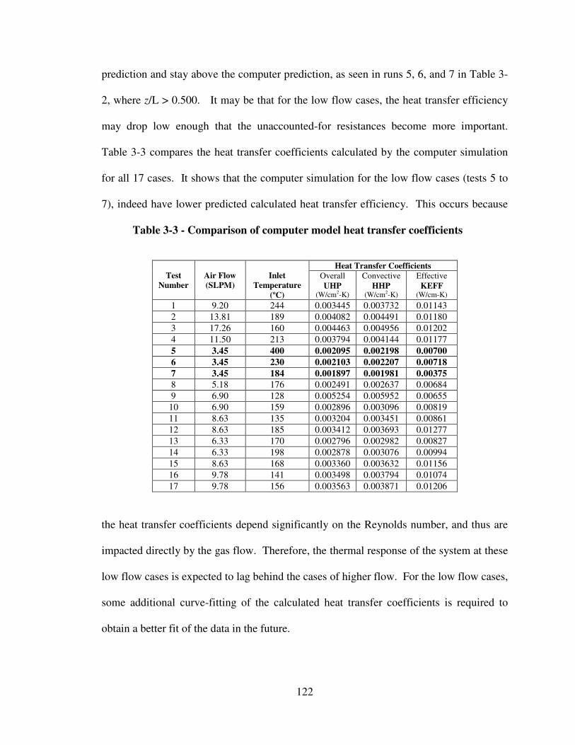
122
prediction and stay above the computer prediction, as seen in runs 5, 6, and 7 in Table 3-
2, where z/L > 0.500. It may be that for the low flow cases, the heat transfer efficiency
may drop low enough that the unaccounted-for resistances become more important.
Table 3-3 compares the heat transfer coefficients calculated by the computer simulation
for all 17 cases. It shows that the computer simulation for the low flow cases (tests 5 to
7), indeed have lower predicted calculated heat transfer efficiency. This occurs because
Table 3-3 - Comparison of computer model heat transfer coefficients
Test
Number
Air Flow
(SLPM)
Inlet
Temperature
(ºC)
Heat Transfer Coefficients
Overall
UHP (W/cm2-K)
Convective
HHP (W/cm2-K)
Effective
KEFF (W/cm-K)
1 9.20 244 0.003445 0.003732 0.01143
2 13.81 189 0.004082 0.004491 0.01180
3 17.26 160 0.004463 0.004956 0.01202
4 11.50 213 0.003794 0.004144 0.01177
5 3.45 400 0.002095 0.002198 0.00700
6 3.45 230 0.002103 0.002207 0.00718
7 3.45 184 0.001897 0.001981 0.00375
8 5.18 176 0.002491 0.002637 0.00684
9 6.90 128 0.005254 0.005952 0.00655
10 6.90 159 0.002896 0.003096 0.00819
11 8.63 135 0.003204 0.003451 0.00861
12 8.63 185 0.003412 0.003693 0.01277
13 6.33 170 0.002796 0.002982 0.00827
14 6.33 198 0.002878 0.003076 0.00994
15 8.63 168 0.003360 0.003632 0.01156
16 9.78 141 0.003498 0.003794 0.01074
17 9.78 156 0.003563 0.003871 0.01206
the heat transfer coefficients depend significantly on the Reynolds number, and thus are
impacted directly by the gas flow. Therefore, the thermal response of the system at these
low flow cases is expected to lag behind the cases of higher flow. For the low flow cases,
some additional curve-fitting of the calculated heat transfer coefficients is required to
obtain a better fit of the data in the future.
123
(3) The remaining data in Table 3-2, for runs 8 on up show the computer simulation to be
a reasonable statistical fit to the actual lab data, except for the aforementioned
temperature difference at z/L = 0.500.
3.6.3 Axial temperature profiles without reaction - While the previous
discussion section reviewed the ability of the computer program to predict the radial
temperature profiles in a ceramic foam catalyst bed under no reaction conditions, the
axial temperature profiles are just as important in assessing the ability of the model to
predict the heat transfer performance of the ceramic catalyst bed. The same experimental
data from the Peng laboratory experiments were compared in the axial direction along the
centerline of the ceramic catalyst bed.
In tabular form, the differences between the lab results and the computer
predictions do not display any obvious patterns. The first 3 comparisons are displayed in
Table 3-4, and, as stated, do not provide an explicit indication of how good or bad the
computer model correlates with the data. For completeness, this same table of individual
comparisons for all 17 lab runs versus the computer model is included in appendix 5.
However, when plotted, against each other, the data versus the computer model
predictions graphically show how they are related. The entire set of all 17 runs of lab
data along the reactor centerline are plotted against the computer model predictions in
Figure 3-13. Here, the laboratory measurements for each run are plotted along the X-
axis, while the corresponding computer model predicted temperature provides the Y-axis
coordinate for the data
.

124
Table 3-4 – Comparison of axial centerline laboratory reactor temps
versus computer simulation results (no reaction present)
Lab
Run
Dimensionless axial distance down the reactor
( z / L )
0.167 0.333 0.500 0.667 0.833
1
Lab Temp,ºK 553 593 623 645 657
Model Temp, ºK 550 598 629 654 692
Delta Temp, ºK -2.67 5.62 5.88 9.82 35.4
% Delta Temp -0.48% 0.95% 0.94% 1.52% 5.38%
2
Lab Temp,ºK 492 530 566 596 617
Model Temp, ºK 477 527 569 606 654
Delta Temp, ºK -14.8 -2.44 3.23 10.1 37.4
% Delta Temp -3.00% -0.46% 0.57% 1.70% 6.05%
3
Lab Temp,ºK 461 496 530 561 586
Model Temp, ºK 437 483 526 566 619
Delta Temp, ºK -24.3 -13.4 -4.40 4.24 32.4
% Delta Temp -5.28% -2.70% -0.83% 0.75% 5.52%
The aggregate correlation of all 17 lab runs versus the computer model provides a
least-squares fit correlation equation (with a forced intercept at [0, 0]) of
�07<CD67< E7FG = 1.0154 × �I;9 J7;KL07< E7FG�, (3-75)
with a correlation coefficient of the entire pooled set of data of R2 = 0.9575. Taken as a
whole, for the entire set of lab data (all 17 runs), both the correlation equation and
correlation coefficient indicate that the computer predicts the heat transfer very closely.
When evaluated individually instead of on a combined basis, the data exhibits
significantly more individual variability. The results for the individual correlation
coefficients range from -0.2230 to 0.9706, as shown in Table 3-5. Table 3-5 shows in
general, high correlation coefficients between the lab data and the computer simulations
for 15 out of the 17 runs. However, runs 5 and 6 show abnormally low correlation
coefficients of 0.223 and 0.629. These 2 runs were then evaluated separately to

125
Figure 3-13 – Lab Axial Temperatures versus Computer Model for all 17 Runs.
determine why their correlation coefficients differ so much from the rest of the data.
For run 5, the axial temperature profile is so flat that the data are clustered very
closely. Figure 3-14 shows that temperature profile along the axis of the reactor spans a
range of only 26ºC, which is the smallest spread in the entire set of 17 lab runs. This is
more apparent when the lab data is plotted against the computer predictions, as in Figure
3-15. However, note earlier in Figure 3-14, that the computer model predicts that the
axial temperature falls off in the second half of the reactor. The reason is that the
externally-applied heat to the shell of the reactor follows the same pattern. Figure 3-16
shows the temperature profiles of the externally-applied heat to the reactor for all 17
laboratory experiments. Run 5 is highlighted in red on this composite plot, and it shows
that the external shell temperature along the axis of the reactor starts out at 410ºC, rises to
459ºC at the mid-point along the reactor, then falls back to 420ºC at the end. The
computer model predicted that the internal temperatures, including the axial values, track
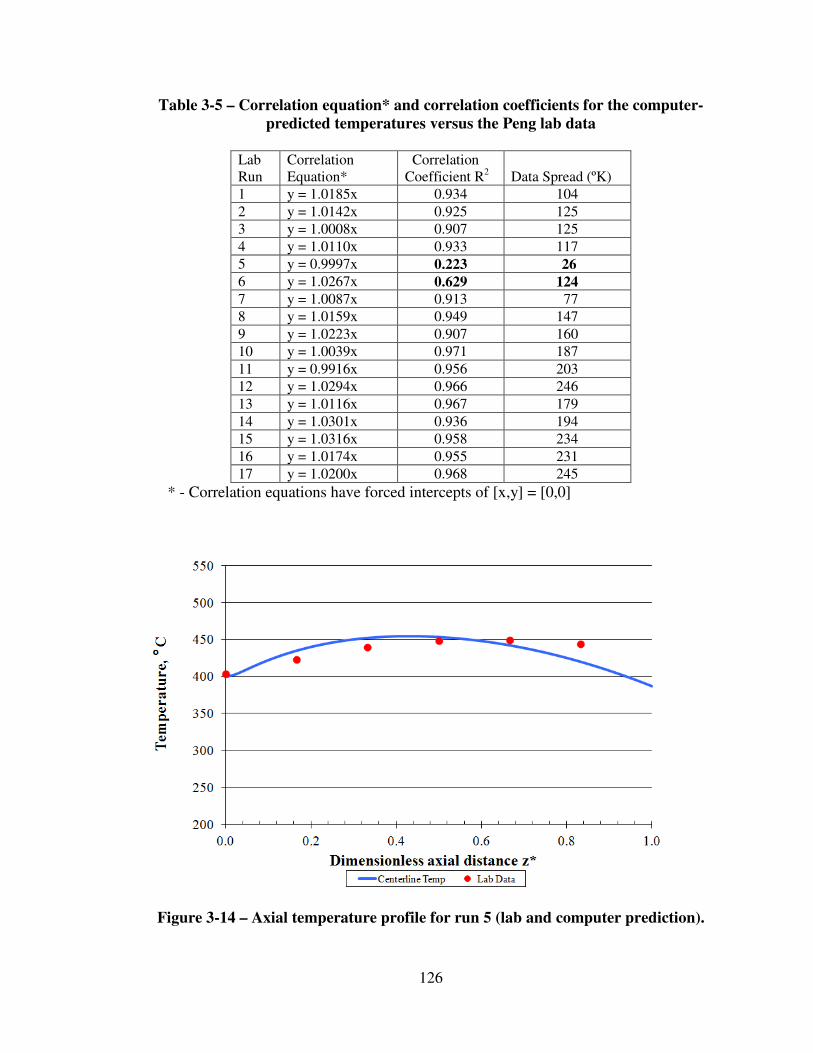
126
Table 3-5 – Correlation equation* and correlation coefficients for the computer-
predicted temperatures versus the Peng lab data
Lab
Run
Correlation
Equation*
Correlation
Coefficient R2
Data Spread (ºK)
1 y = 1.0185x 0.934 104
2 y = 1.0142x 0.925 125
3 y = 1.0008x 0.907 125
4 y = 1.0110x 0.933 117
5 y = 0.9997x 0.223 26
6 y = 1.0267x 0.629 124
7 y = 1.0087x 0.913 77
8 y = 1.0159x 0.949 147
9 y = 1.0223x 0.907 160
10 y = 1.0039x 0.971 187
11 y = 0.9916x 0.956 203
12 y = 1.0294x 0.966 246
13 y = 1.0116x 0.967 179
14 y = 1.0301x 0.936 194
15 y = 1.0316x 0.958 234
16 y = 1.0174x 0.955 231
17 y = 1.0200x 0.968 245
* - Correlation equations have forced intercepts of [x,y] = [0,0]
Figure 3-14 – Axial temperature profile for run 5 (lab and computer prediction).
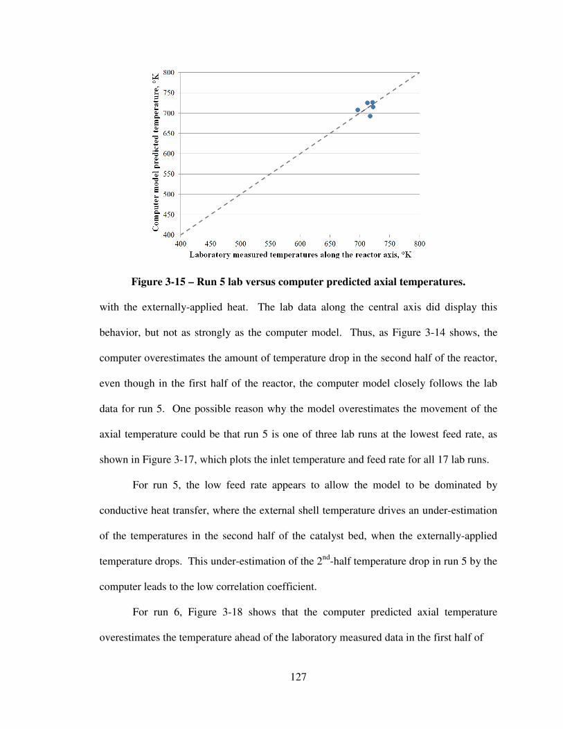
127
Figure 3-15 – Run 5 lab versus computer predicted axial temperatures.
with the externally-applied heat. The lab data along the central axis did display this
behavior, but not as strongly as the computer model. Thus, as Figure 3-14 shows, the
computer overestimates the amount of temperature drop in the second half of the reactor,
even though in the first half of the reactor, the computer model closely follows the lab
data for run 5. One possible reason why the model overestimates the movement of the
axial temperature could be that run 5 is one of three lab runs at the lowest feed rate, as
shown in Figure 3-17, which plots the inlet temperature and feed rate for all 17 lab runs.
For run 5, the low feed rate appears to allow the model to be dominated by
conductive heat transfer, where the external shell temperature drives an under-estimation
of the temperatures in the second half of the catalyst bed, when the externally-applied
temperature drops. This under-estimation of the 2nd
-half temperature drop in run 5 by the
computer leads to the low correlation coefficient.
For run 6, Figure 3-18 shows that the computer predicted axial temperature
overestimates the temperature ahead of the laboratory measured data in the first half of

128
Figure 3-16 – Laboratory external shell temperature profiles (run 5 is highlighted).
Figure 3-17 – Feed rates versus inlet temperatures (run 5 is highlighted).
the reactor, but catches up in the second half of the reactor. There is nothing unusual
about the external shell temperature profile, compared to the other 16 runs. However, run
6 is also one of the lowest feed rate cases, as shown in Figure 3-17. Run 6 suffers the
same issues as run 5, in that the low feed rate allows the conductive heat transfer to domi-
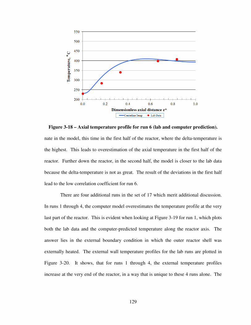
129
Figure 3-18 – Axial temperature profile for run 6 (lab and computer prediction).
nate in the model, this time in the first half of the reactor, where the delta-temperature is
the highest. This leads to overestimation of the axial temperature in the first half of the
reactor. Further down the reactor, in the second half, the model is closer to the lab data
because the delta-temperature is not as great. The result of the deviations in the first half
lead to the low correlation coefficient for run 6.
There are four additional runs in the set of 17 which merit additional discussion.
In runs 1 through 4, the computer model overestimates the temperature profile at the very
last part of the reactor. This is evident when looking at Figure 3-19 for run 1, which plots
both the lab data and the computer-predicted temperature along the reactor axis. The
answer lies in the external boundary condition in which the outer reactor shell was
externally heated. The external wall temperature profiles for the lab runs are plotted in
Figure 3-20. It shows, that for runs 1 through 4, the external temperature profiles
increase at the very end of the reactor, in a way that is unique to these 4 runs alone. The

130
computer model used this boundary condition to drive up the temperatures at the end of
the reactor.
Figure 3-19 - Axial centerline computer simulation results versus lab test number 1.
Figure 3-20 - Laboratory external shell temperature profiles(Runs 1-4 highlighted).
131
3.6.4 Heat transfer conclusions - In general, the heat transfer predictions of the
computer model closely approximate the performance of Peng’s lab reactor. There are
some special cases where low flow causes conductive heat transfer to have more
influence than the convective heat transfer, but as long as the user is aware of these
limitations, the model may be used to make reasonable performance predictions for
design needs.
3.7 Validation of the computer model, methane catalytic combustion
With the computer model able to make reasonable heat transfer predictions, the
next step was to compare the model performance to laboratory experiments which
include the reactions for catalytic combustion of methane. The computer model was
compared to laboratory catalytic combustor data generated by Cantu for ceramic foam
[58]. Cantu conducted catalytic combustion laboratory experiments using a 1 inch (2.54
cm) long, 0.5 inch (1.27 cm) diameter ceramic foam reactor. The reactor vessel used was
a vertical quartz or stainless steel tube with a length of 23.5 inches (59.7 cm) and an inner
diameter of 0.5 inches (1.27 cm). The reactor tube was much longer than the catalyst in
order to minimize end effects. Figure 3-21 shows the layout of this lab reactor. Thirteen
specific laboratory experiments, as shown in Table 3-6, were used for comparison.
When the same operating conditions of the 13 lab runs in Table 3-6 were inputted
to the computer model, the results in Table 3-7 were obtained. The reaction equation was
first order in methane, and the kinetic constants used for all the computer runs were the
same: Ea (activation energy) equal to 155.9 kJ mol-1
, and a pre-exponential factor k0 equal
to 95,980 mol atm-1
sec-1
cm-3
. The results show that the computer model reasonably
predicts the conversion of methane (CH4). A plot of the results in Table 3-7 in Figure 3-

132
22 graphically shows how well-correlated the predicted conversion of the computer
Figure 3-21 – Lab reactor for testing ceramic foam combustor.
Table 3-6 – Laboratory experimental data with catalytic methane combustion
Laboratory
CH4
conversion
(%)
CH4 feed Feed
Reactor
wall
rate temp temp
(stdcm3/min) (ºC) (ºC)
Case 1 6.98 545 562 5.63
6.98 594 610 13.8
6.98 643 660 34.5
6.98 693 710 69.0
6.98 748 761 96.1
Case 2 9.75 546 563 4.81
9.75 644 661 28.0
9.75 694 712 64.2
9.75 752 764 94.7
Case 3 13.7 537 558 2.79
13.7 593 610 7.44
13.7 696 712 58.5
13.7 747 762 94.5

133
is to the actual laboratory data. In this figure, each curve corresponds to a given case (1,
2, or 3) with a fixed feed rate, but with different feed and external boundary condition
temperatures. The correlation coefficients are all greater than 0.98, indicating excellent
correlation of the computer prediction to the actual lab data.
Table 3-7 – Laboratory experimental conversion vs. computer model predictions
Laboratory
actual CH4
conversion
(%)
Model
CH4 feed predicted CH4
rate conversion
(stdcm3/min) (%)
Case 1 6.98 5.63 5.07
6.98 13.8 16.6
6.98 34.5 43.6
6.98 69.0 80.2
6.98 96.1 97.2
Case 2 9.75 4.81 3.77
9.75 28.0 34.2
9.75 64.2 69.7
9.75 94.7 95.8
Case 3 13.7 2.79 2.35
13.7 7.44 8.70
13.7 58.5 58.1
13.7 94.5 88.7
Figure 3-22 - Computer predictions of the combustor conversion vs.
actual lab data.
134
With the model able to closely demonstrate the measured laboratory results, from
the heat transfer and methane conversion standpoints, the computer model is now used to
optimize design conditions for a scaled-up commercial unit.
3.8 Parametric studies of the combustor model
To better understand the model response to changes in its inputted parameters,
and whether those responses follow expected behavior or not, a parametric study of the
current model was undertaken. Prior parametric studies of catalytic combustion of
methane on ceramic foam computer model by Cantu evaluated the effects of changing
keff, Der, Tw, T0, and Bi [58]. The key measure of the impact of these parameter changes
was the maximum catalyst bed temperature. One of the main objectives of this study was
to minimize bed temperature to lower NOx emissions. Therefore, parameter changes
which lowered the bed temperature were advantageous for reducing NOx. For each of
these five parameters, the following conclusions were reached:
(1) keff – Higher values of the effective thermal conductivity lead to lower maximum bed
temperatures because the risk of forming a thermal hot spot is lower as the ability of the
bed to conduct heat away is increased.
(2) Der – Increasing the effective mass diffusivity in the radial direction was found to
steeply reduce the maximum bed temperature, Tmax, up to a point. After this point of
lowest maximum bed temperature, further increases of Der would result in gradual
increases of Tmax. This point of lowest Tmax was found to be at Der = 8.0 × 10⁻⁵
m2s
-1.
(3) Tw – As the reactor wall temperature increases, the maximum bed temperature, Tmax,
increases. Overall reactor conversion also increases, but there is a point at which the
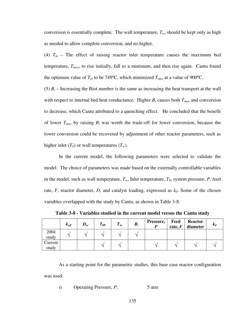
135
conversion is essentially complete. The wall temperature, Tw, should be kept only as high
as needed to allow complete conversion, and no higher.
(4) Tin – The effect of raising reactor inlet temperature causes the maximum bed
temperature, Tmax, to rise initially, fall to a minimum, and then rise again. Cantu found
the optimum value of Tin to be 749ºC, which minimized Tmax at a value of 900ºC.
(5) Bi – Increasing the Biot number is the same as increasing the heat transport at the wall
with respect to internal bed heat conductance. Higher Bi causes both Tmax and conversion
to decrease, which Cantu attributed to a quenching effect. He concluded that the benefit
of lower Tmax by raising Bi was worth the trade-off for lower conversion, because the
lower conversion could be recovered by adjustment of other reactor parameters, such as
higher inlet (T0) or wall temperatures (Tw).
In the current model, the following parameters were selected to validate the
model. The choice of parameters was made based on the externally controllable variables
in the model, such as wall temperature, Tw, Inlet temperature, T0, system pressure, P, feed
rate, F, reactor diameter, D, and catalyst loading, expressed as k0. Some of the chosen
variables overlapped with the study by Cantu, as shown in Table 3-8.
Table 3-8 - Variables studied in the current model versus the Cantu study
keff Der THP Tin Bi Pressure,
P
Feed
rate, F
Reactor
diameter k0
2004
study √ √ √ √ √
Current
study √ √ √ √ √ √
As a starting point for the parametric studies, this base case reactor configuration
was used:
i) Operating Pressure, P: 5 atm
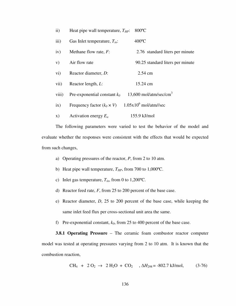
136
ii) Heat pipe wall temperature, THP: 800ºC
iii) Gas Inlet temperature, Tin: 400ºC
iv) Methane flow rate, F: 2.76 standard liters per minute
v) Air flow rate 90.25 standard liters per minute
vi) Reactor diameter, D: 2.54 cm
vii) Reactor length, L: 15.24 cm
viii) Pre-exponential constant k0 13,600 mol/atm/sec/cm3
ix) Frequency factor (k0 × V) 1.05x10⁶ mol/atm//sec
x) Activation energy Ea 155.9 kJ/mol
The following parameters were varied to test the behavior of the model and
evaluate whether the responses were consistent with the effects that would be expected
from such changes,
a) Operating pressures of the reactor, P, from 2 to 10 atm.
b) Heat pipe wall temperature, THP, from 700 to 1,000ºC.
c) Inlet gas temperature, Tin, from 0 to 1,200ºC.
d) Reactor feed rate, F, from 25 to 200 percent of the base case.
e) Reactor diameter, D, 25 to 200 percent of the base case, while keeping the
same inlet feed flux per cross-sectional unit area the same.
f) Pre-exponential constant, k0, from 25 to 400 percent of the base case.
3.8.1 Operating Pressure – The ceramic foam combustor reactor computer
model was tested at operating pressures varying from 2 to 10 atm. It is known that the
combustion reaction,
CH4 + 2 O2 → 2 H2O + CO2 , ∆H298 = -802.7 kJ/mol, (3-76)
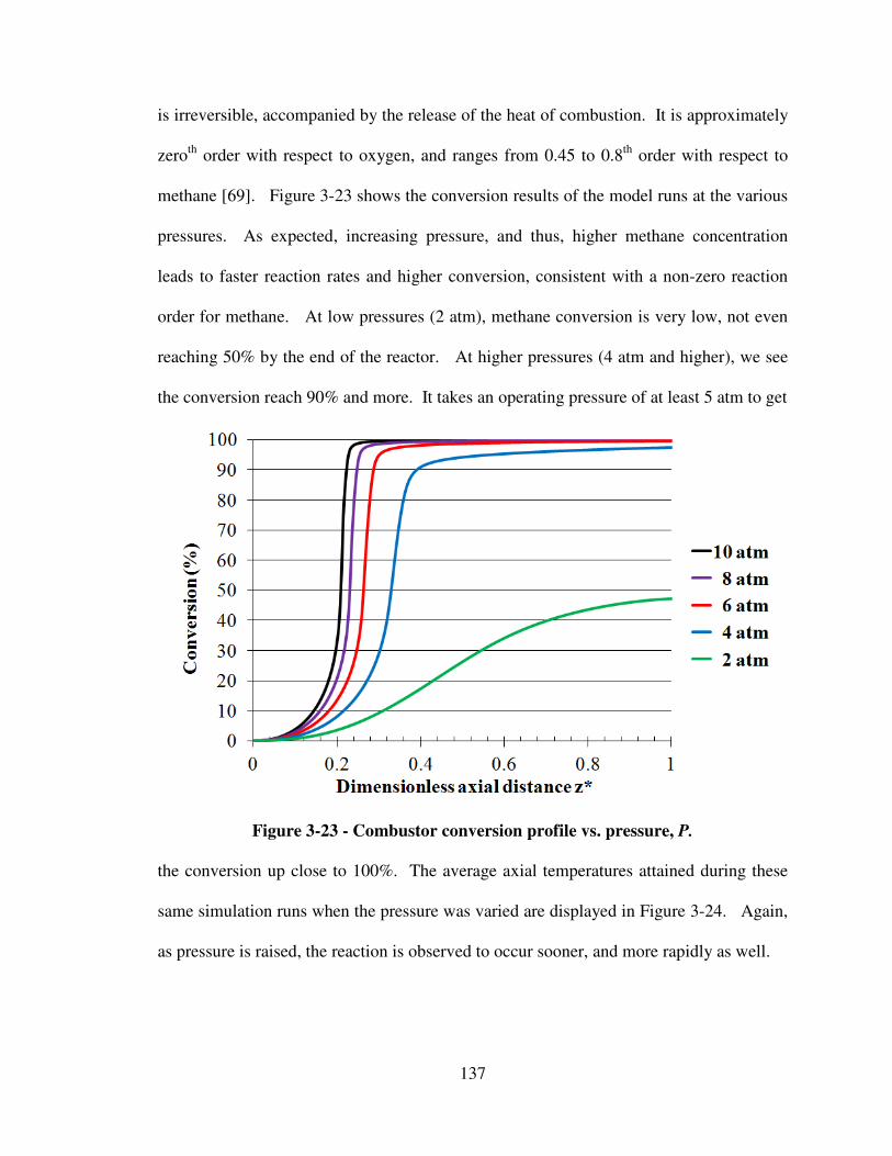
137
is irreversible, accompanied by the release of the heat of combustion. It is approximately
zeroth
order with respect to oxygen, and ranges from 0.45 to 0.8th
order with respect to
methane [69]. Figure 3-23 shows the conversion results of the model runs at the various
pressures. As expected, increasing pressure, and thus, higher methane concentration
leads to faster reaction rates and higher conversion, consistent with a non-zero reaction
order for methane. At low pressures (2 atm), methane conversion is very low, not even
reaching 50% by the end of the reactor. At higher pressures (4 atm and higher), we see
the conversion reach 90% and more. It takes an operating pressure of at least 5 atm to get
Figure 3-23 - Combustor conversion profile vs. pressure, P.
the conversion up close to 100%. The average axial temperatures attained during these
same simulation runs when the pressure was varied are displayed in Figure 3-24. Again,
as pressure is raised, the reaction is observed to occur sooner, and more rapidly as well.
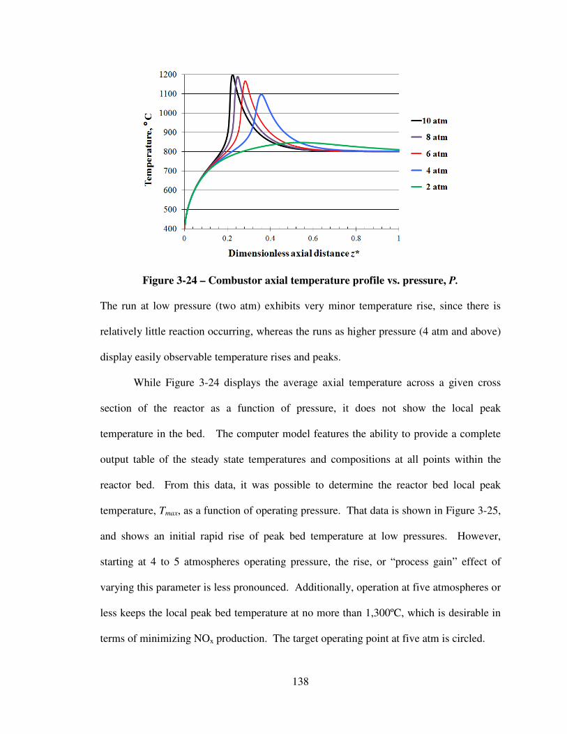
138
Figure 3-24 – Combustor axial temperature profile vs. pressure, P.
The run at low pressure (two atm) exhibits very minor temperature rise, since there is
relatively little reaction occurring, whereas the runs as higher pressure (4 atm and above)
display easily observable temperature rises and peaks.
While Figure 3-24 displays the average axial temperature across a given cross
section of the reactor as a function of pressure, it does not show the local peak
temperature in the bed. The computer model features the ability to provide a complete
output table of the steady state temperatures and compositions at all points within the
reactor bed. From this data, it was possible to determine the reactor bed local peak
temperature, Tmax, as a function of operating pressure. That data is shown in Figure 3-25,
and shows an initial rapid rise of peak bed temperature at low pressures. However,
starting at 4 to 5 atmospheres operating pressure, the rise, or “process gain” effect of
varying this parameter is less pronounced. Additionally, operation at five atmospheres or
less keeps the local peak bed temperature at no more than 1,300ºC, which is desirable in
terms of minimizing NOx production. The target operating point at five atm is circled.
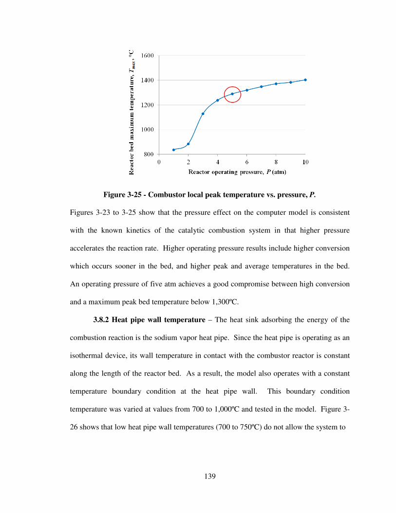
139
Figure 3-25 - Combustor local peak temperature vs. pressure, P.
Figures 3-23 to 3-25 show that the pressure effect on the computer model is consistent
with the known kinetics of the catalytic combustion system in that higher pressure
accelerates the reaction rate. Higher operating pressure results include higher conversion
which occurs sooner in the bed, and higher peak and average temperatures in the bed.
An operating pressure of five atm achieves a good compromise between high conversion
and a maximum peak bed temperature below 1,300ºC.
3.8.2 Heat pipe wall temperature – The heat sink adsorbing the energy of the
combustion reaction is the sodium vapor heat pipe. Since the heat pipe is operating as an
isothermal device, its wall temperature in contact with the combustor reactor is constant
along the length of the reactor bed. As a result, the model also operates with a constant
temperature boundary condition at the heat pipe wall. This boundary condition
temperature was varied at values from 700 to 1,000ºC and tested in the model. Figure 3-
26 shows that low heat pipe wall temperatures (700 to 750ºC) do not allow the system to

140
Figure 3-26 – Combustor conversion profile vs. heat pipe wall temperature, THP .
reach full conversion. By contrast, higher heat pipe temperatures (800ºC and above)
allow conversion to rise close to completion. The average axial temperatures of the
reactor bed for these runs with varying heat pipe temperature are shown in Figure 3-27.
Although higher heat pipe temperatures raise the conversion and cause it to occur sooner
as well, an additional impact, seen is that maximum average axial temperature rises with
higher heat pipe wall temperature. For the run at 900ºC, average axial temperature
exceeds 1200ºC, which presents issues with NOx generation in combustor operation.
Further evidence that 900ºC is too high for catalytic combustor operation comes from
examining the local maximum bed temperature, plotted in Figure 3-28. We see in Figure
3-28 that the peak local bed temperature exceeds 1,500ºC when the reactor wall
temperature is 900ºC. For this reason, an upper limit of 800ºC on the heat pipe wall

141
Figure 3-27 - Combustor axial temperature vs. heat pipe wall temperature, THP .
temperature is proposed. This limits the reactor bed local maximum temperature to
1,290ºC, and is also a good match for a heat pipe using metallic sodium as its working
Figure 3-28 - Combustor local peak temperature vs. reactor wall temperature, THP .
fluid, since the vapor pressure of sodium at 800ºC is approximately 0.5 atm. The
optimum operating point in Figure 3-28 is circled.
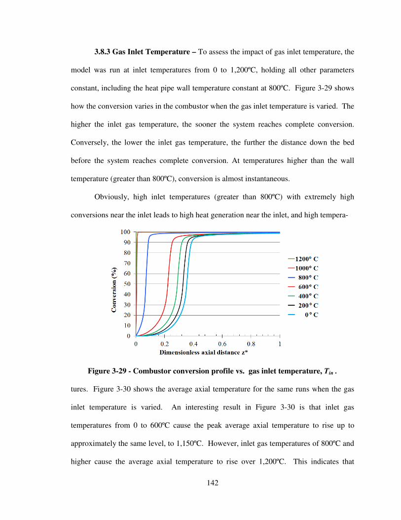
142
3.8.3 Gas Inlet Temperature – To assess the impact of gas inlet temperature, the
model was run at inlet temperatures from 0 to 1,200ºC, holding all other parameters
constant, including the heat pipe wall temperature constant at 800ºC. Figure 3-29 shows
how the conversion varies in the combustor when the gas inlet temperature is varied. The
higher the inlet gas temperature, the sooner the system reaches complete conversion.
Conversely, the lower the inlet gas temperature, the further the distance down the bed
before the system reaches complete conversion. At temperatures higher than the wall
temperature (greater than 800ºC), conversion is almost instantaneous.
Obviously, high inlet temperatures (greater than 800ºC) with extremely high
conversions near the inlet leads to high heat generation near the inlet, and high tempera-
Figure 3-29 - Combustor conversion profile vs. gas inlet temperature, Tin .
tures. Figure 3-30 shows the average axial temperature for the same runs when the gas
inlet temperature is varied. An interesting result in Figure 3-30 is that inlet gas
temperatures from 0 to 600ºC cause the peak average axial temperature to rise up to
approximately the same level, to 1,150ºC. However, inlet gas temperatures of 800ºC and
higher cause the average axial temperature to rise over 1,200ºC. This indicates that

143
operating at inlet temperatures below 600ºC stay within the capabilities of the system to
transfer enough thermal energy that the average axial bed temperature does not exceed
1,150ºC. However, inlet temperatures of 800ºC and higher create conditions where the
reaction is fast enough that convection and conduction are not enough to keep the average
axial bed temperature below 1,200ºC.
The lower the peak temperature in the bed, the lower the risk of creating NOx
emissions from the system. The peak axial average temperature is kept below 1,150ºC if
Figure 3-30 - Combustor axial temperature profile vs. gas inlet temperature, Tin .
the inlet temperature can be held at 600ºC or less.
Concerning the reactor bed peak temperature, Tmax, as a function of inlet
temperature, an interesting phenomenon is displayed in Figure 3-31. The reactor bed
local peak temperature is fairly constant at approximately 1,290ºC at inlet temperatures
below 750ºC. It then begins to rise at inlet temperatures starting at 800ºC. Figures 3-29,
3-30, and 3-31 indicate that inlet temperatures from 200 to 400ºC meet the performance
requirements of high conversion, while at the same time keeps peak local bed

144
temperatures below 1,300ºC, minimizing the risk of NOx formation. The “process gain”
on local bed peak temperature as function of inlet temperature in the range of 200 to
400ºC is zero, meaning there is no observed effect. The preferred operating point of
400ºC is circled on Figure 3-31.
Figure 3-31 - Combustor local peak temperature vs. inlet temperature, Tin .
3.8.4 Reactor feed rates – To assess the effect of feed rate, the gas feed rates
were varied from 25% to 200% of the baseline case. At lower feed rates, the combustion
reactor reached always reached its peak conversion sooner, and also attained a higher
total conversion. Figure 3-32 shows the conversion profiles resulting from these runs.
For low feed rates (less than 100% of the base case) the inward radial heat transfer from
the heat pipe wall transfer heat better into the ceramic foam bed and heats it to the “light-
off” temperature earlier, since the axial convective heat transfer is lower for the lower
feed rate cases. As a result, the lower feed rate “lights-off” sooner and reaches a higher
ultimate conversion. Conversely, in the higher rate cases (greater than 100% of the base
case), the convective forces delay the point of “light-off,” and also result in lower overall
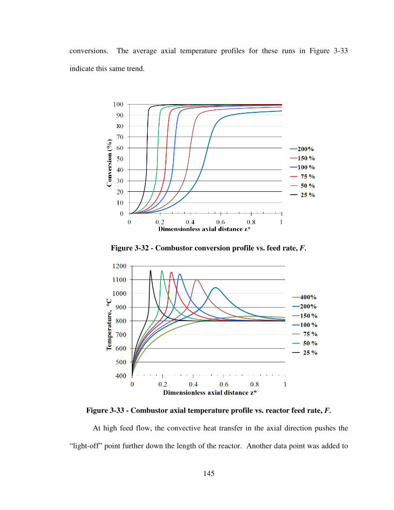
145
conversions. The average axial temperature profiles for these runs in Figure 3-33
indicate this same trend.
Figure 3-32 - Combustor conversion profile vs. feed rate, F.
Figure 3-33 - Combustor axial temperature profile vs. reactor feed rate, F.
At high feed flow, the convective heat transfer in the axial direction pushes the
“light-off” point further down the length of the reactor. Another data point was added to

146
Figure 3-33 at 400% of the base case. At this highest feed rate case, the “light-off” point
was so far down the reactor bed that it is beyond the outlet. In such cases, the axial
convective forces are overwhelming the ability of the inward radial heat conduction to
heat the reactor to the “light-off” point. An example of this is shown in Figure 3-33 when
the feed rate is increased to 400% of the baseline flow. The reaction front never has an
opportunity to develop, and high conversion is unobtainable. The reactor never gets an
opportunity to warm up to the “light-off” temperature, so it is no surprise that the
conversion is low.
When examining the local peak reactor bed temperatures for these cases in Figure
3-34, a similar trend is evident, i.e. the higher feed rates result in lower peak
temperatures. Higher convection drives the resulting peak temperature lower and further
down the bed. The slope of Figure 3-34, which is the “process gain” of the feed rate
Figure 3-34 - Combustor local peak temperature vs. reactor feed rate, F.
impact on local bed peak temperature is relatively steady, meaning there are no sudden
changes to the local bed peak temperature as feed rate is adjusted. This steadiness
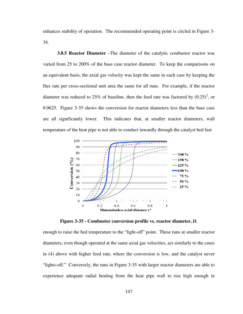
147
enhances stability of operation. The recommended operating point is circled in Figure 3-
34.
3.8.5 Reactor Diameter –The diameter of the catalytic combustor reactor was
varied from 25 to 200% of the base case reactor diameter. To keep the comparisons on
an equivalent basis, the axial gas velocity was kept the same in each case by keeping the
flux rate per cross-sectional unit area the same for all runs. For example, if the reactor
diameter was reduced to 25% of baseline, then the feed rate was factored by (0.25)2, or
0.0625. Figure 3-35 shows the conversion for reactor diameters less than the base case
are all significantly lower. This indicates that, at smaller reactor diameters, wall
temperature of the heat pipe is not able to conduct inwardly through the catalyst bed fast
Figure 3-35 - Combustor conversion profile vs. reactor diameter, D.
enough to raise the bed temperature to the “light-off” point. These runs at smaller reactor
diameters, even though operated at the same axial gas velocities, act similarly to the cases
in (4) above with higher feed rate, where the conversion is low, and the catalyst never
“lights-off.” Conversely, the runs in Figure 3-35 with larger reactor diameters are able to
experience adequate radial heating from the heat pipe wall to rise high enough in

148
temperature to “light-off” and go to essentially complete conversion. There is a curious
side effect to this trend if the reactor diameter is increased indefinitely: As the diameter
of the reactor is increased from 100% on up to 200% in Figure 3-36 the distance down
the bed where complete conversion occurs is greater. This occurs because the larger
diameter reactors have more methane to react, longer radial distances for the thermal
energy from the wall to penetrate into the bed, and increased thermal masses of the larger
diameter bed before light-off conditions are met. This means that light-off happens
further on down the bed. Additionally, the average axial temperature profiles for these
runs in Figure 3-36 shows more evidence that smaller diameter reactors are unable to
achieve significant temperatures to aid higher conversion, while the larger diameter
reactors achieve near complete conversion further down the bed.
When the reactor bed peak local temperatures are plotted as a function of reactor
diameter as in Figure 3-37, an S-shaped curve is obtained, in which inflection points are
revealed both below and above the base case. The inflection points can be taken to
indicate changes in controlling mechanisms in the reactor. Below the inflection point
(less than 75% reactor diameter), the reactor bed never achieves high enough
temperatures to “light-off.”
Between the two inflection points, Figure 3-37 points to the diameter range of 75
to 150% of the base case for a region of relatively slower “process gain” with respect to
the peak local bed temperatures, making for more stable operation. It is also
advantageous to keep the base case diameter of 100% of the reactor diameter, which will
limit the peak local bed temperature to 1,290ºC and minimize NOx formation.
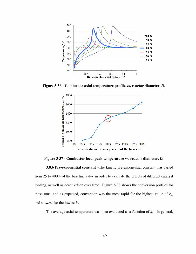
149
Figure 3-36 - Combustor axial temperature profile vs. reactor diameter, D.
Figure 3-37 - Combustor local peak temperature vs. reactor diameter, D.
3.8.6 Pre-exponential constant –The kinetic pre-exponential constant was varied
from 25 to 400% of the baseline value in order to evaluate the effects of different catalyst
loading, as well as deactivation over time. Figure 3-38 shows the conversion profiles for
these runs, and as expected, conversion was the most rapid for the highest value of k0,
and slowest for the lowest k0.
The average axial temperature was then evaluated as a function of k0. In general,
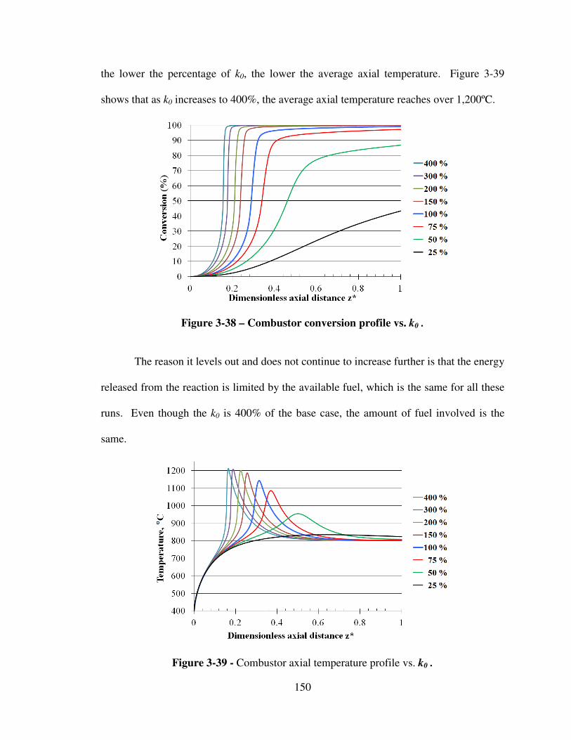
150
the lower the percentage of k0, the lower the average axial temperature. Figure 3-39
shows that as k0 increases to 400%, the average axial temperature reaches over 1,200ºC.
Figure 3-38 – Combustor conversion profile vs. k0 .
The reason it levels out and does not continue to increase further is that the energy
released from the reaction is limited by the available fuel, which is the same for all these
runs. Even though the k0 is 400% of the base case, the amount of fuel involved is the
same.
Figure 3-39 - Combustor axial temperature profile vs. k0 .

151
Finally, the local bed peak temperature was evaluated as a function of k0. In this
case, the local bed peak temperature continues to rise as k0 increases, since the local rate
of reaction also increases. There is an initial steep increase of the local peak bed
temperature, but that smoothes out to a lesser rate of increase at 100% of the base case
and beyond. Thereafter, the “process gain” is smaller, and operation in this region is
more stable than at lower values of k0, as shown in Figure 3-40.
Figure 3-40 - Local peak temperature as a function of k0 .
3.8.7 Summary of combustor parametric evaluation – Table 3-9 summarizes
the evaluation of important parameters.
Table 3-9 - Summary of the variables studied in the combustor parametric study Range tested
Parameter Units Lower
limit
Upper
limit
Baseline
conditions
Operating Pressure, P atmospheres 1 10 5
Heat Pipe wall temperature, Tw (M C) 700 1,000 800
Inlet gas temperature, Tin (M C) 0 1,200 400
Reactor Feed rate, F (% of base case) 25 200 100
Reactor diameter, D (% of base case) 25 200 100
Pre-exponential factor, k0 (% of base case) 25 400 100
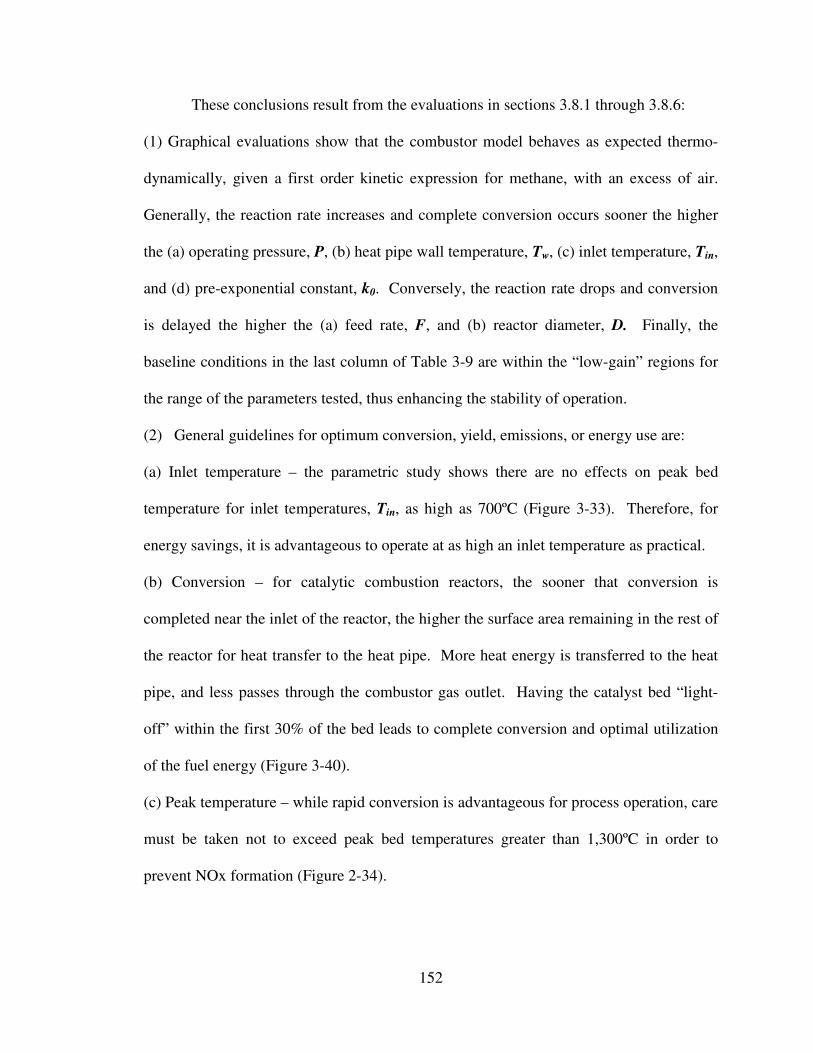
152
These conclusions result from the evaluations in sections 3.8.1 through 3.8.6:
(1) Graphical evaluations show that the combustor model behaves as expected thermo-
dynamically, given a first order kinetic expression for methane, with an excess of air.
Generally, the reaction rate increases and complete conversion occurs sooner the higher
the (a) operating pressure, P, (b) heat pipe wall temperature, Tw, (c) inlet temperature, Tin,
and (d) pre-exponential constant, k0. Conversely, the reaction rate drops and conversion
is delayed the higher the (a) feed rate, F, and (b) reactor diameter, D. Finally, the
baseline conditions in the last column of Table 3-9 are within the “low-gain” regions for
the range of the parameters tested, thus enhancing the stability of operation.
(2) General guidelines for optimum conversion, yield, emissions, or energy use are:
(a) Inlet temperature – the parametric study shows there are no effects on peak bed
temperature for inlet temperatures, Tin, as high as 700ºC (Figure 3-33). Therefore, for
energy savings, it is advantageous to operate at as high an inlet temperature as practical.
(b) Conversion – for catalytic combustion reactors, the sooner that conversion is
completed near the inlet of the reactor, the higher the surface area remaining in the rest of
the reactor for heat transfer to the heat pipe. More heat energy is transferred to the heat
pipe, and less passes through the combustor gas outlet. Having the catalyst bed “light-
off” within the first 30% of the bed leads to complete conversion and optimal utilization
of the fuel energy (Figure 3-40).
(c) Peak temperature – while rapid conversion is advantageous for process operation, care
must be taken not to exceed peak bed temperatures greater than 1,300ºC in order to
prevent NOx formation (Figure 2-34).

153
(d) Heat pipe wall temperature – this is limited by the choice of heat pipe working fluid.
Fortunately, sodium heat pipes operate well at 800ºC, where steam reforming is efficient.
(e) Reactor diameter – enlarging the diameter excessively leads to overly-long thermal
conduction paths from the center of the catalyst bed to the heat pipe wall. This creates
enough higher thermal resistance and raises the risk of excessively-high peak bed
temperatures.
3.9 Parametric studies of the reformer model
A parametric evaluation of the reformer computer model was performed to assess
its sensitivity to input variables, and to validate whether the model reacted as expected to
these changes.
3.9.1 Reforming reaction - The computer model for the reformer features
kinetics based on four factors; (1) the catalyst operates at such high temperatures that the
deposited active metal catalyst is sufficiently active without need for a washcoat, (2) pore
diffusion is neglected because the equivalent spherical diameter for the 30 PPI foam of
0.83 mm is less than 1 mm, as shown in Table 3-10, (3) the forward reaction is well
represented by first-order kinetics with the methane concentration,
Rate = k0 × Exp(-Ea/(RT)) × (yCH4PTot ) mol/s ·g cat [51] , and (3-77)
(4) the reverse reaction can be accounted for by modifying the rate equation to
Rate = k0 × Exp(-Ea/(RT)) × (yCH4PTot –3
32
2
H COTot
SRH O
y yP
y K ) mol/s ·g cat [51]
, (3-78)
where KSR is the reforming reaction equilibrium constant, represented as
[ ]
322
4 2
1/ exp(25390 / 27.776) 51 .H COSR TOT
CH H O
y yK P T
y y= = −
(3-79)

154
The rate equations in Equations 3-77 through 3-79 were determined during an earlier
phase of heat pipe reactor research at the University of Houston [51]. They were
obtained from measurements on a crushed sample of industrial catalyst containing 14
wt% Ni/Al2O3, and these rate equations were used in the current research as
representative of a typical example of a catalyst. In the current research, model work,
and reformer parametric evaluation, catalytic activity was adjusted by varying the pre-
exponential constant, k0. If a different catalyst were to be used, its rate equation and
reaction constants would have to be validated experimentally.
Table 3-10 – Ceramic foam physical properties [55,57]
Pores per inch dp
foam pore
diameter (mm)
Sv external surface
area (m2m(solid)
-3)
ds pellet equivalent
diameter (mm)
10 1.5 1.76×10⁴ 0.34
30 0.83 2.62×10⁴ 0.23
80 0.02 12.30×10⁴ 0.05
The following parameters were selected to validate the model, based on the
externally controllable variables in the program; (1) system operating pressure P, (2) wall
temperature THP, (3) Inlet temperature Tin, (4) feed rate F, (5) reactor diameter, D, and (6)
catalyst activity, expressed as k0.
3.9.2 Operating pressure – Reformer pressures at 2.5 atm, 5 atm, and 7.5 atm
were evaluated in the reformer model. Because the reforming reaction is equilibrium-
limited and produces more moles of gas in the forward direction, higher operating
pressures favor the reverse reaction towards fewer moles of gas in the system, per Le
Chatelier’s Principle. The conversion plots at different operating pressures in Figure 3-
41 demonstrates that the model follows Le Chatelier’s Principle, as higher pressure
operation leads to lower conversion at all axial points in the reformer, while lower

155
pressure results in higher conversion. The targeted operating pressure is five atm. The
reformer average axial temperature response at different pressures reacts as expected
when factoring in the conversion attained and the positive enthalpy of the endothermic
reforming reaction. At low pressure operation, the higher conversion of the endothermic
reaction adsorbs more energy from the catalyst bed, lowering its average axial
temperature, as seen in Figure 3-42. This is true for the first 70% of the bed length as
seen in Figure 3-42, where the reforming reaction rate is significant. However very little
reaction occurs in the last 30% of the bed length, so the low pressure case axial
temperature profile actually crosses the higher pressure cases due to thermal conduction
from the reactor wall to the bed, as seen in Figure 3-43.
Figure 3-41 – Reformer conversion profile vs. pressure, P.
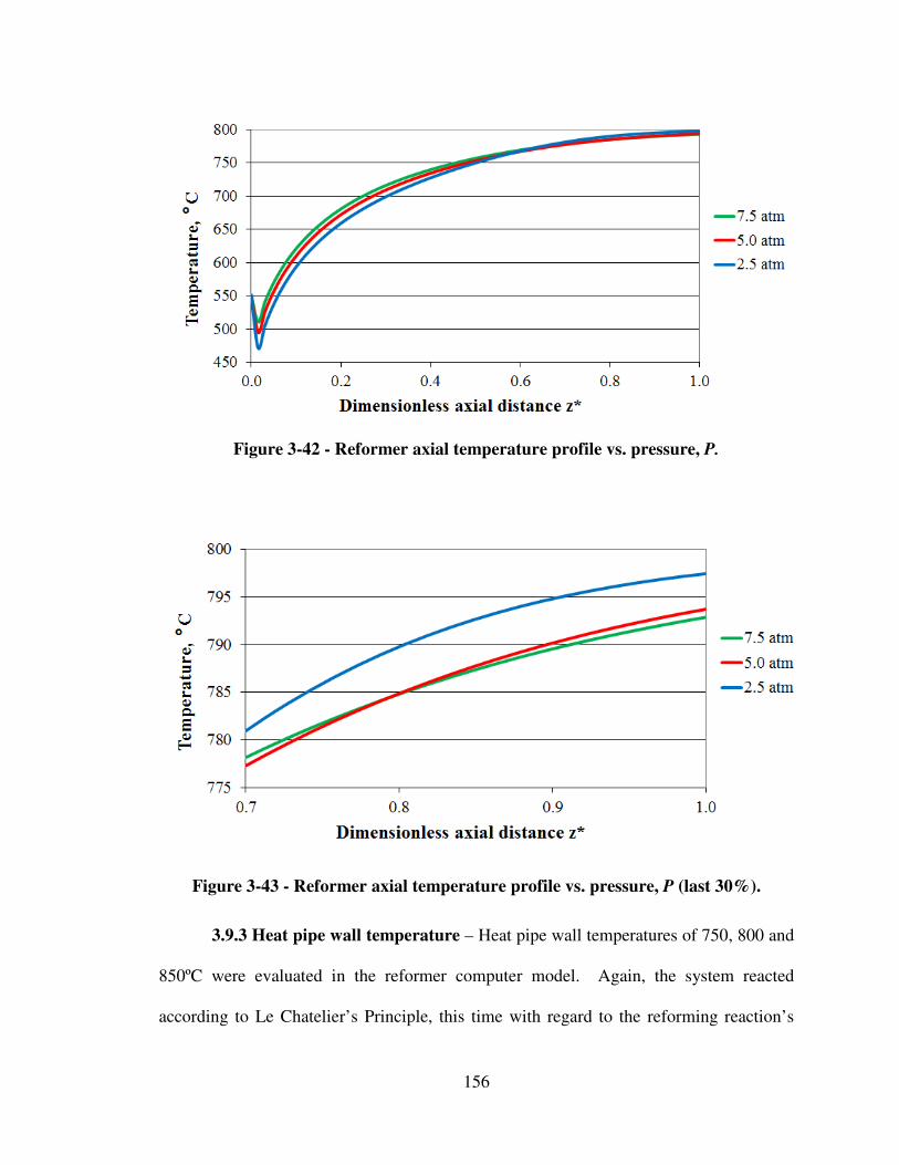
156
Figure 3-42 - Reformer axial temperature profile vs. pressure, P.
Figure 3-43 - Reformer axial temperature profile vs. pressure, P (last 30%).
3.9.3 Heat pipe wall temperature – Heat pipe wall temperatures of 750, 800 and
850ºC were evaluated in the reformer computer model. Again, the system reacted
according to Le Chatelier’s Principle, this time with regard to the reforming reaction’s

157
endothermic enthalpy. At higher temperature, conversion of an endothermic reaction will
also increase, as shown in Figure 3-44.
Figure 3-44 – Reformer conversion profile vs. heat pipe wall temperature, THP .
The average axial temperature of the reformer when operated at temperatures
follows this same trend that higher heat pipe wall temperatures lead to higher catalyst bed
temperatures, as shown in Figure 3-45.
Figure 3-45 – Reformer axial temperature profile vs. heat pipe wall
temperature, THP .
3.9.4 Gas inlet temperature – Gas inlet temperatures of 450, 551, and 650ºC
were tested in the reformer computer model. The thermal mass of the inlet gases is

158
insignificant compared to that of the catalyst bed and reactor, so the inlet gas temperature
does not have any significant effect on conversion in Figure 3-46, or on axial average bed
temperature in Figure 3-47.
Figure 3-46 - Reformer conversion profile vs. gas inlet temperature, Tin .
Figure 3-47 - Reformer axial temperature profile vs. gas inlet temperature, Tin .
3.9.5 Reactor feed rates – Methane feed rates of 75, 150, and 300 SLPM were
evaluated in the reformer computer model. The conversion profile of the low flow 75
SLPM case is higher than the 150 SLPM base flow case as expected due to higher
residence time in the reactor, allowing more energy to be adsorbed by the endothermic
reforming reaction, pushing conversion higher. The conversion profile of the 300 SLPM
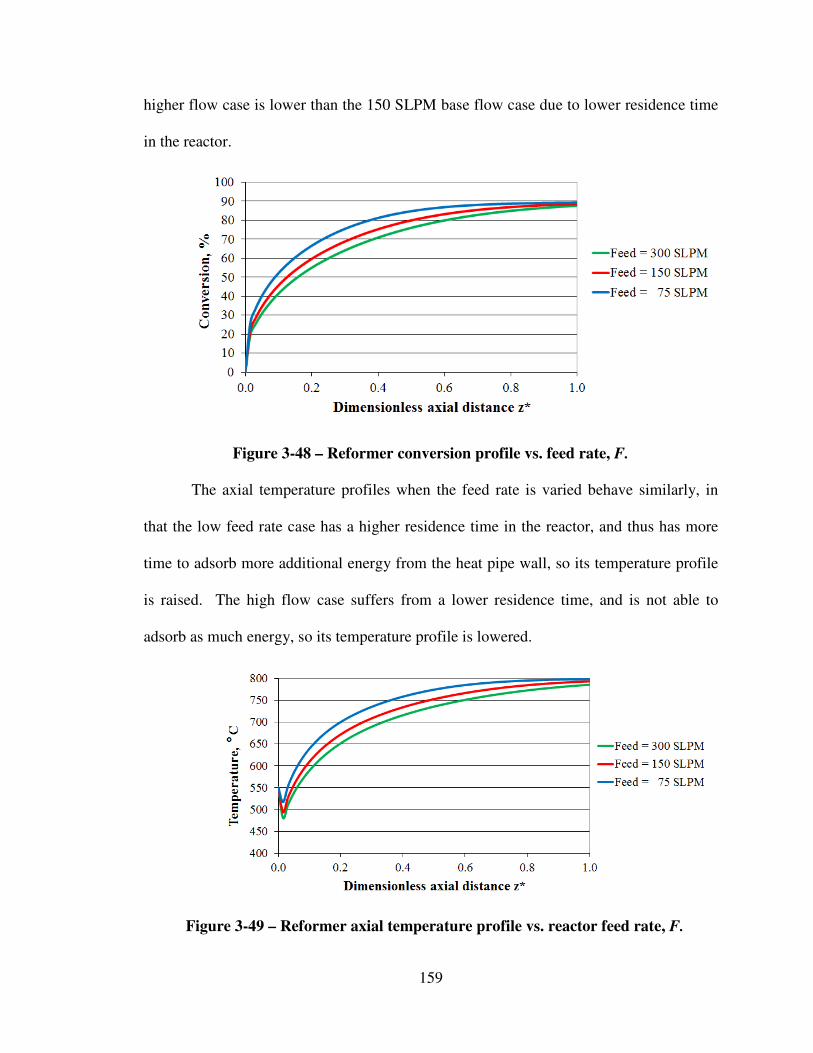
159
higher flow case is lower than the 150 SLPM base flow case due to lower residence time
in the reactor.
Figure 3-48 – Reformer conversion profile vs. feed rate, F.
The axial temperature profiles when the feed rate is varied behave similarly, in
that the low feed rate case has a higher residence time in the reactor, and thus has more
time to adsorb more additional energy from the heat pipe wall, so its temperature profile
is raised. The high flow case suffers from a lower residence time, and is not able to
adsorb as much energy, so its temperature profile is lowered.
Figure 3-49 – Reformer axial temperature profile vs. reactor feed rate, F.
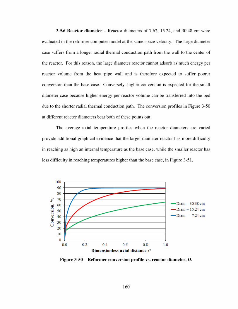
160
3.9.6 Reactor diameter – Reactor diameters of 7.62, 15.24, and 30.48 cm were
evaluated in the reformer computer model at the same space velocity. The large diameter
case suffers from a longer radial thermal conduction path from the wall to the center of
the reactor. For this reason, the large diameter reactor cannot adsorb as much energy per
reactor volume from the heat pipe wall and is therefore expected to suffer poorer
conversion than the base case. Conversely, higher conversion is expected for the small
diameter case because higher energy per reactor volume can be transferred into the bed
due to the shorter radial thermal conduction path. The conversion profiles in Figure 3-50
at different reactor diameters bear both of these points out.
The average axial temperature profiles when the reactor diameters are varied
provide additional graphical evidence that the larger diameter reactor has more difficulty
in reaching as high an internal temperature as the base case, while the smaller reactor has
less difficulty in reaching temperatures higher than the base case, in Figure 3-51.
Figure 3-50 – Reformer conversion profile vs. reactor diameter, D.

161
Figure 3-51 - Reformer axial temperature profile vs. reactor diameter, D.
3.9.7 Pre-exponential constant – The kinetic pre-exponential constant k0 for the
reforming reaction was evaluated at 2.22, 4.44, and 8.88 gm-moles·atm-1
sec-1
cm-3
. At
low values of k0 which indicate low catalyst activity, the conversion should fall, as shown
in Figure 3-52. If a more active catalyst with a higher k0 were installed, the conversion
profile would rise with it, also seen in Figure 3-52.
Figure 3-52 – Reformer conversion profile vs. k0 .
The axial temperature profiles are also affected by k0. At low k0, Figure 3-53
shows that there is a less pronounced dip in the temperature early in the bed because the
endothermic reaction is significantly less, so less energy is being adsorbed. For high k0,
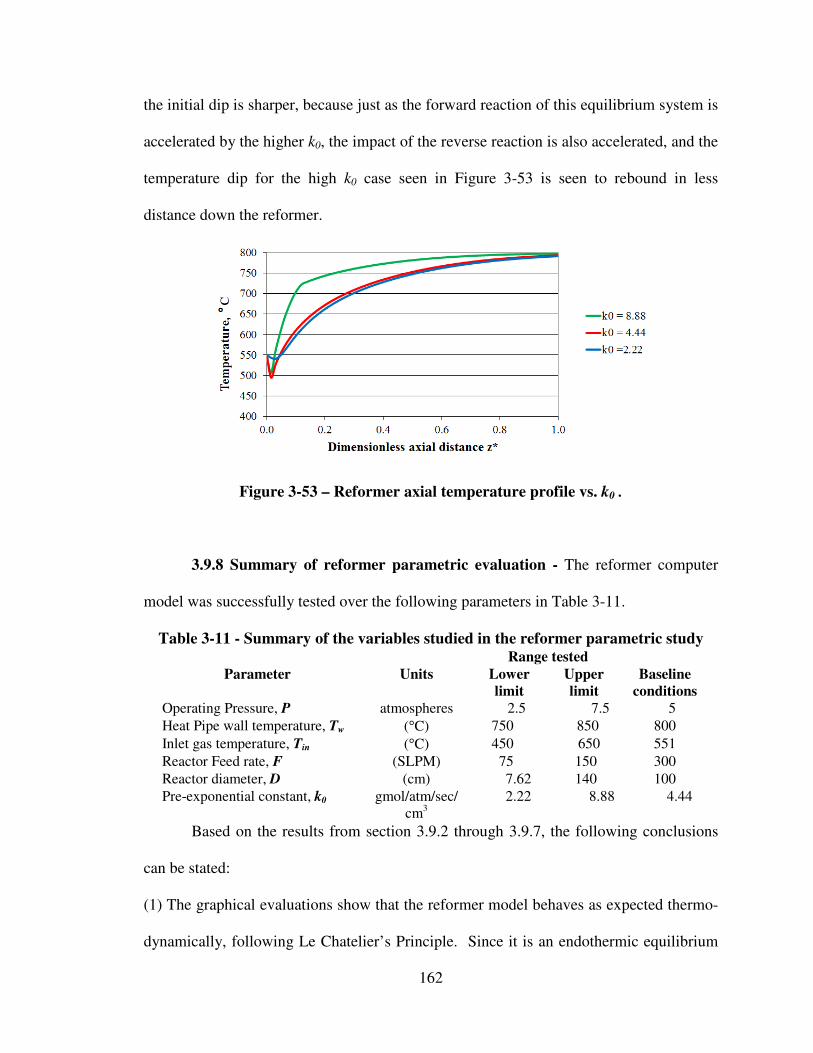
162
the initial dip is sharper, because just as the forward reaction of this equilibrium system is
accelerated by the higher k0, the impact of the reverse reaction is also accelerated, and the
temperature dip for the high k0 case seen in Figure 3-53 is seen to rebound in less
distance down the reformer.
Figure 3-53 – Reformer axial temperature profile vs. k0 .
3.9.8 Summary of reformer parametric evaluation - The reformer computer
model was successfully tested over the following parameters in Table 3-11.
Table 3-11 - Summary of the variables studied in the reformer parametric study Range tested
Parameter Units Lower
limit
Upper
limit
Baseline
conditions
Operating Pressure, P atmospheres 2.5 7.5 5
Heat Pipe wall temperature, Tw (°C) 750 850 800
Inlet gas temperature, Tin (°C) 450 650 551
Reactor Feed rate, F (SLPM) 75 150 300
Reactor diameter, D (cm) 7.62 140 100
Pre-exponential constant, k0 gmol/atm/sec/
cm3
2.22 8.88 4.44
Based on the results from section 3.9.2 through 3.9.7, the following conclusions
can be stated:
(1) The graphical evaluations show that the reformer model behaves as expected thermo-
dynamically, following Le Chatelier’s Principle. Since it is an endothermic equilibrium
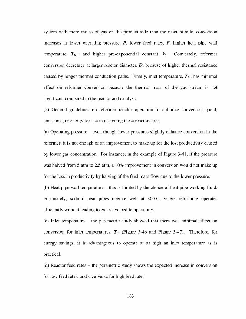
163
system with more moles of gas on the product side than the reactant side, conversion
increases at lower operating pressure, P, lower feed rates, F, higher heat pipe wall
temperature, THP, and higher pre-exponential constant, k0. Conversely, reformer
conversion decreases at larger reactor diameter, D, because of higher thermal resistance
caused by longer thermal conduction paths. Finally, inlet temperature, Tin, has minimal
effect on reformer conversion because the thermal mass of the gas stream is not
significant compared to the reactor and catalyst.
(2) General guidelines on reformer reactor operation to optimize conversion, yield,
emissions, or energy for use in designing these reactors are:
(a) Operating pressure – even though lower pressures slightly enhance conversion in the
reformer, it is not enough of an improvement to make up for the lost productivity caused
by lower gas concentration. For instance, in the example of Figure 3-41, if the pressure
was halved from 5 atm to 2.5 atm, a 10% improvement in conversion would not make up
for the loss in productivity by halving of the feed mass flow due to the lower pressure.
(b) Heat pipe wall temperature – this is limited by the choice of heat pipe working fluid.
Fortunately, sodium heat pipes operate well at 800ºC, where reforming operates
efficiently without leading to excessive bed temperatures.
(c) Inlet temperature – the parametric study showed that there was minimal effect on
conversion for inlet temperatures, Tin (Figure 3-46 and Figure 3-47). Therefore, for
energy savings, it is advantageous to operate at as high an inlet temperature as is
practical.
(d) Reactor feed rates – the parametric study shows the expected increase in conversion
for low feed rates, and vice-versa for high feed rates.

164
(e) Reactor diameter – enlarging the diameter excessively can lead to overly-long thermal
conduction paths from the center of the catalyst bed to the heat pipe wall. This creates
enough additional thermal resistance that limits conversion (Figure 3-50).
(f) Pre-exponential constant – managing the activity of the catalyst is essential to
maintaining the productivity of the system. Known poisons that affect reforming catalyst
life must be controlled and prevented from adversely affecting its activity.
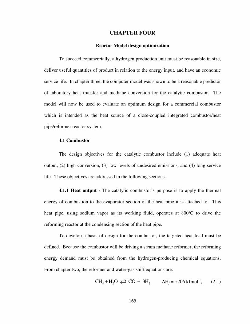
165
CHAPTER FOUR
Reactor Model design optimization
To succeed commercially, a hydrogen production unit must be reasonable in size,
deliver useful quantities of product in relation to the energy input, and have an economic
service life. In chapter three, the computer model was shown to be a reasonable predictor
of laboratory heat transfer and methane conversion for the catalytic combustor. The
model will now be used to evaluate an optimum design for a commercial combustor
which is intended as the heat source of a close-coupled integrated combustor/heat
pipe/reformer reactor system.
4.1 Combustor
The design objectives for the catalytic combustor include (1) adequate heat
output, (2) high conversion, (3) low levels of undesired emissions, and (4) long service
life. These objectives are addressed in the following sections.
4.1.1 Heat output - The catalytic combustor’s purpose is to apply the thermal
energy of combustion to the evaporator section of the heat pipe it is attached to. This
heat pipe, using sodium vapor as its working fluid, operates at 800ºC to drive the
reforming reactor at the condensing section of the heat pipe.
To develop a basis of design for the combustor, the targeted heat load must be
defined. Because the combustor will be driving a steam methane reformer, the reforming
energy demand must be obtained from the hydrogen-producing chemical equations.
From chapter two, the reformer and water-gas shift equations are:
4 2 2CH H O CO 3H+ +�
∆Hf = +206 kJmol
-1, (2-1)
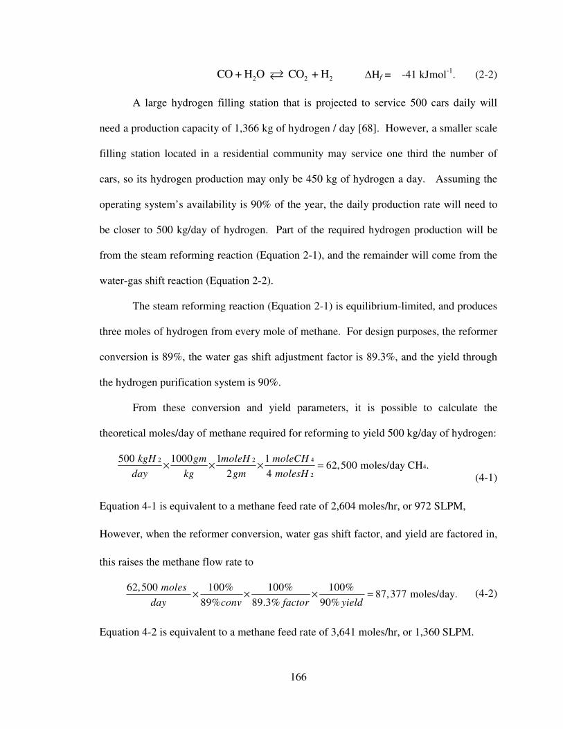
166
2 2 2CO + H O CO + H� ∆Hf = -41 kJmol
-1. (2-2)
A large hydrogen filling station that is projected to service 500 cars daily will
need a production capacity of 1,366 kg of hydrogen / day [68]. However, a smaller scale
filling station located in a residential community may service one third the number of
cars, so its hydrogen production may only be 450 kg of hydrogen a day. Assuming the
operating system’s availability is 90% of the year, the daily production rate will need to
be closer to 500 kg/day of hydrogen. Part of the required hydrogen production will be
from the steam reforming reaction (Equation 2-1), and the remainder will come from the
water-gas shift reaction (Equation 2-2).
The steam reforming reaction (Equation 2-1) is equilibrium-limited, and produces
three moles of hydrogen from every mole of methane. For design purposes, the reformer
conversion is 89%, the water gas shift adjustment factor is 89.3%, and the yield through
the hydrogen purification system is 90%.
From these conversion and yield parameters, it is possible to calculate the
theoretical moles/day of methane required for reforming to yield 500 kg/day of hydrogen:
2 2 44
2
500 1000 1 1 62,500 moles/day CH .
2 4
kgH gm moleH moleCH
day kg gm molesH× × × =
(4-1)
Equation 4-1 is equivalent to a methane feed rate of 2,604 moles/hr, or 972 SLPM,
However, when the reformer conversion, water gas shift factor, and yield are factored in,
this raises the methane flow rate to
62,500 100% 100% 100%87,377 moles/day.
89% 89.3% 90%
moles
day conv factor yield× × × =
(4-2)
Equation 4-2 is equivalent to a methane feed rate of 3,641 moles/hr, or 1,360 SLPM.

167
The enthalpy requirement for this reaction load in the reformer with 89% conversion, is
41,360 206 60 min89% 668 MJ/hr,
22.4 1000
LitersCH kJ mol MJ
Minute mol L hr kJ× × × × × = (4-3)
that the combustor has to provide to drive the reforming system.
The combustion reaction is exothermic with a large negative enthalpy of reaction,
CH4 + 2 O2 � CO2 + 2 H2O(g) ∆Hf = -802.27 kJmol-1
. (4-4)
To generate the required energy load of 668 MJ/hr (186 kW) requires a methane
combustion rate of
4668 1000 22.4
60 min 802.27
MJ hr molCH kJ L
hr kJ MJ mole× × × × = 311 SLPM CH4 . (4-5)
For convenience, the combustor stoichiometric methane flow design basis from this point
onward will be taken as one-twelfth of this flow, or 25.9 SLPM. Each combustor reactor
will then need to theoretically deliver 186 kW / 12, or 15.5 kW of energy for reforming.
With this as a basis, the full-scale system to meet the 500 kg hydrogen/day production
requirement will need twelve such systems in parallel.
While the theoretical heat load per reactor just to drive reforming is 15.5 kW,
additional heat loads further burden the combustor. For instance, a prime safety concern
is to operate the combustor at less than the lower explosive limit (LFL) for methane in air
in case of gas leaks in the system. This requires at least 20 parts of air for every part
methane to keep the mixture below the LEL of 5 volume %. The target 33 to 1 air to
methane ratio requires significant energy to raise the air up to the catalytic combustion
temperature. A heat balance shows that the energy to raise this quantity of air from
ambient conditions to catalytic combustion temperature requires 14.4 kW per reactor,
which is almost equal to the 15.5 kW load just for reforming. For design purposes, the

168
combustor heat duty will be doubled to 31 kW per reactor and will require a methane
feed rate of 51.8 SLPM. Results in chapter six will show that this design criterion is
within ±5% of the true required combustor heat load.
The catalytic combustor computer model which was developed in chapter three
utilized a methane flow rate of 0.545 SLPM methane/cm2 of reactor cross sectional area
and a diameter to length aspect ratio of 1 to 6. Scaling up the combustor model for the
reformer’s designed heat load (QReformer) of 31 kW at a methane feed rate of 51.8 SLPM
leads to a diameter of 11 cm (4.33 inches) and length of 66 cm (26 inches). This
configuration provides a space velocity of 8.25 min-1
.
A non-standard reactor diameter of 11 cm (4.33 inches) is more costly to build
than a more common size. Therefore, this reactor will be enlarged to fit within a standard
15.24 cm (6 inch) diameter pipe. Keeping the same space velocity of 8.25 min-1
leads to
a reactor length of 34.4 cm (13.5 inches). The energy delivered by such a reactor is equal
to 25.8 kW. It is significantly less than 31 kW due to 5.2 kW of energy lost out the exit
of the combustor because the exit temperature is 933ºC, as seen in the axial average
temperature profile of this reactor in Figure 4-1. The high exit temperature is the cause
of the 5.2 kW of energy loss which is not deliverable to the heat pipe. It is so high
because the reactor length of 34.4 cm (13.5 inches) is too short to provide adequate heat
transfer area between the reactor and heat pipe. Recall that this length was calculated for
a given cross-sectional area by keeping the same space velocity of 8.25 min-1
as the lab
reactor.

169
The solution to lowering the heat lost out the exit of the combustor due to
excessive reactor gas exit temperature is to relax the space velocity requirement and
Figure 4-1 - Average axial temperature for the short ( 34.4 cm) combustor.
allow the reactor to be lengthened to increase the surface area for heat transfer between
the reactor and heat pipe. Lengthening the combustor to 100 cm, almost triples the heat
transfer area to the heat pipe. The effect of lengthening the reactor decreases the space
velocity from 8.25 min-1
to 2.8 min-1
. The benefit can be seen in the lower reactor exit
temperature of 822ºC seen in the axial temperature profile of Figure 4-2. The heat lost in
the exit has dropped from 5.2 kW down to 0.7 kW. This leaves 30.3 kW available to the
heat pipe which is within 2% of our initial criteria of 31 kW.
The heat balance for the integrated combustor / heat pipe is tabulated in Table 4-
1. It shows again how the sensible heat load of the combustor can consume almost half
of the energy generated in the combustor.
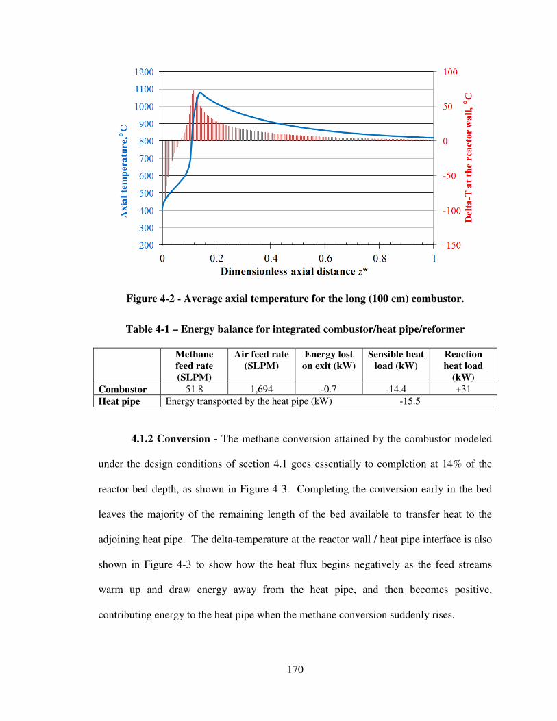
170
Figure 4-2 - Average axial temperature for the long (100 cm) combustor.
Table 4-1 – Energy balance for integrated combustor/heat pipe/reformer
Methane
feed rate
(SLPM)
Air feed rate
(SLPM)
Energy lost
on exit (kW)
Sensible heat
load (kW)
Reaction
heat load
(kW)
Combustor 51.8 1,694 -0.7 -14.4 +31
Heat pipe Energy transported by the heat pipe (kW) -15.5
4.1.2 Conversion - The methane conversion attained by the combustor modeled
under the design conditions of section 4.1 goes essentially to completion at 14% of the
reactor bed depth, as shown in Figure 4-3. Completing the conversion early in the bed
leaves the majority of the remaining length of the bed available to transfer heat to the
adjoining heat pipe. The delta-temperature at the reactor wall / heat pipe interface is also
shown in Figure 4-3 to show how the heat flux begins negatively as the feed streams
warm up and draw energy away from the heat pipe, and then becomes positive,
contributing energy to the heat pipe when the methane conversion suddenly rises.
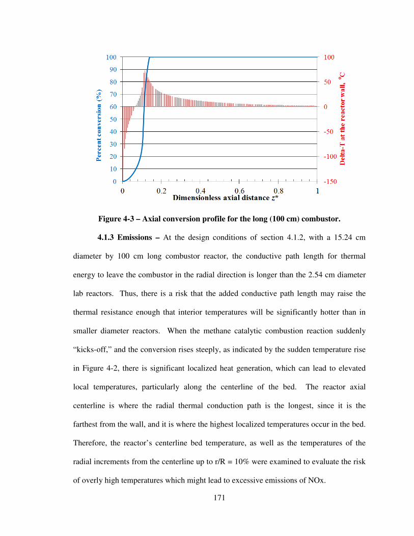
171
Figure 4-3 – Axial conversion profile for the long (100 cm) combustor.
4.1.3 Emissions – At the design conditions of section 4.1.2, with a 15.24 cm
diameter by 100 cm long combustor reactor, the conductive path length for thermal
energy to leave the combustor in the radial direction is longer than the 2.54 cm diameter
lab reactors. Thus, there is a risk that the added conductive path length may raise the
thermal resistance enough that interior temperatures will be significantly hotter than in
smaller diameter reactors. When the methane catalytic combustion reaction suddenly
“kicks-off,” and the conversion rises steeply, as indicated by the sudden temperature rise
in Figure 4-2, there is significant localized heat generation, which can lead to elevated
local temperatures, particularly along the centerline of the bed. The reactor axial
centerline is where the radial thermal conduction path is the longest, since it is the
farthest from the wall, and it is where the highest localized temperatures occur in the bed.
Therefore, the reactor’s centerline bed temperature, as well as the temperatures of the
radial increments from the centerline up to r/R = 10% were examined to evaluate the risk
of overly high temperatures which might lead to excessive emissions of NOx.

172
Recall from section 2.10 and Figure 2-34, that combustion temperatures in the
presence of excess air above 1300ºC significantly raise the possibility of NOx formation.
From Figure 2-34, a table of the expected NOx concentration as a function of gas
temperature can be created, as in Table 4-2. Curve fitting the data of Table 4-2 yields the
Table 4-2 – Expected NOx concentration as a function of gas temperature
Gas temperature
(°C)
NO concentration
(ppmvw)
1,000 0
1,100 0
1,200 0
1,300 25
1,400 100
1,500 190
1,600 350
following equation for NOx formation as a function of temperature:
NOx ( )5 34.467 10 exp 273 8.559 10o
ppmvw T C− − = × + × ×
. (4-6)
The combustor final design case in the above section leads to a high peak bed
temperature of 1,423ºC at an axial distance of l/L = 0.14 at r/R = 0.06 in the reactor. The
centerline temperature axial profile, as well as the temperature profiles at radial distances
from r/R = 2% to r/R = 10% are plotted in Figure 4-4. Further away from the centerline,
the peak temperatures are lower, lowering the risk of creating NOx. Equation 4-6 was
used to calculate a concentration profile of NOx in the radial direction at l/L = 0.14, taken
as the hottest spot in the reactor bed, in order to calculate an average NOx concentration
across the face of the reactor.
The radial NOx concentration profile is shown in Figure 4-5, and the averaged
NOx concentration across the face of reactor when normalized by surface area calculates

173
Figure 4-4 - Axial temperature profiles at different radial distances for the
combustor.
out to 3.9 ppmvw of NOx. For a system of twelve combustors operating in parallel, each
with a methane feed rate of 51.8 SLPM per reactor and an air feed rate of 1,694 SLPM
for 90 % of the year, this results in a NOx emission of 113 lbs./year. This amount of
NOx emissions over a year is comparable to that emitted by 3 passenger cars [83], and
must be evaluated against local ordinances to determine whether additional emissions
controls are necessary.
Figure 4-5 – Radial NOx concentration profile for the heat pipe combustor.
174
4.1.4 Service life - As catalyst beds age, the catalyst activity at the stationary
active reaction front drops, causing the reaction front to shift position further and further
on down the bed. The rapidity at which this occurs is a function of the purity of feed
streams to the combustor, and how many catalyst poisons are present.
The larger concern, however, is that if the design basis for the combustor design
counts on having adequate reactor to heat pipe surface area to transport enough heat to
drive the reformer, this surface area will be encroached upon as the catalyst bed ages and
the active reaction front progresses downward through the bed. This may mean that the
catalyst bed may need to be upsized even more to accommodate the expected age
deterioration of the catalyst, while still maintaining the heat generating capacity to drive
the reformer. Future work will have to be conducted to get a better estimate of the
combustor catalyst life so that this can be factored into the sizing basis of the system.
4.1.5 Combustor Summary - Optimization of the combustor to meet the energy
needs of the reformer has brought about a firm design for the combustor reactor of 15.24
cm diameter and 100 cm in length. It has also resulted in a methane demand in the
combustor of 51.8 SLPM, which is twice the theoretical amount of 25.9 SLPM needed to
drive the production of hydrogen in the reformer. This difference arose from not taking
into account the sensible heat loads in bringing reactant feed gases up to operating
temperature, and by taking into account conversion and yield in the reformer. Finalizing
the heat balances brought the realization that additional energy was needed to operate at
the heat pipe temperatures of 800ºC. The additional energy does not have to be wasted
out the flue gas stack. It can be recovered for preheating of the feeds, or for steam export
or electricity generation.
175
4.2 Reformer
From section 4.1, the hydrogen production sizing basis for the reformer is 500
kg/day / 12, or 41.7 kg/day of hydrogen per reactor. This requires a theoretical methane
feed rate to the reformer of 972 SLPM / 12, or 81 SLPM, with a steam feed rate of 243
SLPM (Equation 4-1). However, since conversion does not go to completion in
reformers because the reaction is equilibrium-limited, the actual reformer feed rate must
be up-rated to account for less than 100% conversion. Additionally, there is a hydrogen
yield loss across the hydrogen purification system of 10%, which is recycled back to the
combustor. For a reformer operating at 5 atm pressure and 800ºC, the equilibrium
conversion is taken to be approximately 89%. Therefore, the actual reformer feed rate to
meet the daily hydrogen production target, taking into account the equilibrium conversion
and yield loss, is 1,360 SLPM /12, or 113.3 SLPM of methane, and 340 SLPM of steam
per reactor.
4.2.1 Reformer sizing - The reformer computer model used a methane feed rate
basis of 1.275 SLPM of methane fed per cm2 of reformer cross sectional area, with a
space velocity of 4.27 min-1
. With this feed rate basis and space velocity of 4.27 min-1
,
113.3 SLPM of methane requires a minimum reformer diameter of 10.6 cm (4.2 inches)
and length of 299 cm (118 inches). However, since the combustor bed in section 4.1 was
sized at 15.24 cm (6 inches) in diameter, it is advantageous from a construction cost
standpoint to size the reformer at the same diameter of 15.24 cm. Also, space constraints
limit the available length of the reformer. The computer model was run using a diameter
of 15.24 cm at various bed lengths to verify whether adequate conversion was still
attainable with a shorter reformer vessel. The model evaluation runs at the various bed

176
lengths are tabulated in Table 4-3. The criteria for success is when the last column of
Table 4-3 is equal to or greater than 102 SLPM of net methane conversion in the
reformer, which allows for a 10% yield loss through the hydrogen purification system.
The results show a reactor length of 2 m is required to satisfy the net conversion
success criteria of 102 SLPM of methane in the last column of Table 4-3.
Table 4-3 - Computer model evaluation of 15.24 cm diameter reformer
Diameter
(cm)
Length
(m)
Conversion
(%)
CH4 feed
(SLPM)
Net conversion x
CH4 (SLPM)
15.24
0.5 69.2
113.3
78.4
0.75 78.5 88.9
1.0 83.8 94.9
1.25 86.7 98.2
1.50 88.2 99.9
1.75 88.9 100.7
2.0 89.2 101.1
4.2.2 Conversion - Figure 4-6 shows conversion as a function of distance down
the length of the 2 m reformer. The last half of the conversion profile, (Z > 1 m) shows a
relatively flat progression of conversion, indicating that the system is conservatively
sized, and would not deteriorate in performance as quickly if this profile were steeper. At
the beginning of the conversion profile, it has an initial steep linear rise, then changes at
Z = 0.03 m to a smoothly increasing curve until the end of the reactor, where is reaches
its maximum of 89.2% conversion. The initial steep linear rise before Z reaches 0.03 m
occurs because the forward reaction of conversion of methane into hydrogen (Equation 2-
1) has not yet reached equilibrium with the reverse reaction. Until enough products have
accumulated to where the reverse reaction becomes significant, the forward reaction
progresses very rapidly. It only takes until Z = 0.03 m for the reverse reaction to become
significant.
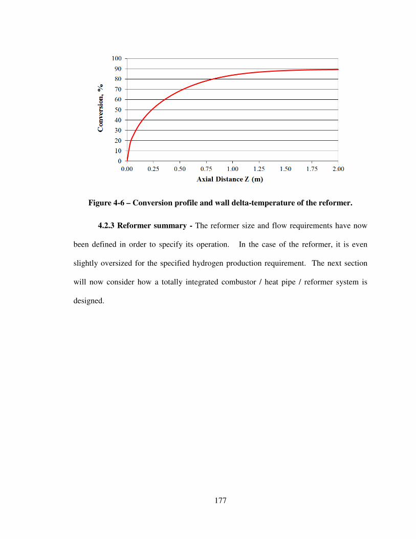
177
Figure 4-6 – Conversion profile and wall delta-temperature of the reformer.
4.2.3 Reformer summary - The reformer size and flow requirements have now
been defined in order to specify its operation. In the case of the reformer, it is even
slightly oversized for the specified hydrogen production requirement. The next section
will now consider how a totally integrated combustor / heat pipe / reformer system is
designed.
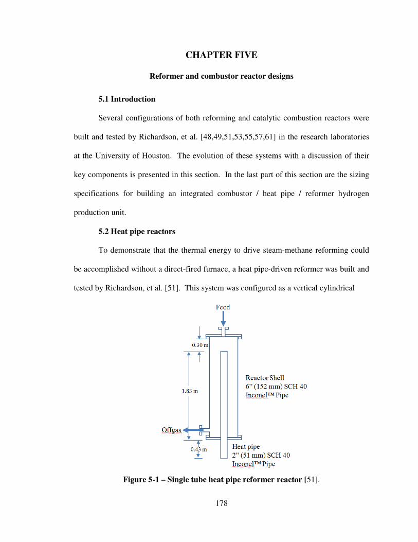
178
CHAPTER FIVE
Reformer and combustor reactor designs
5.1 Introduction
Several configurations of both reforming and catalytic combustion reactors were
built and tested by Richardson, et al. [48,49,51,53,55,57,61] in the research laboratories
at the University of Houston. The evolution of these systems with a discussion of their
key components is presented in this section. In the last part of this section are the sizing
specifications for building an integrated combustor / heat pipe / reformer hydrogen
production unit.
5.2 Heat pipe reactors
To demonstrate that the thermal energy to drive steam-methane reforming could
be accomplished without a direct-fired furnace, a heat pipe-driven reformer was built and
tested by Richardson, et al. [51]. This system was configured as a vertical cylindrical
Figure 5-1 – Single tube heat pipe reformer reactor [51].
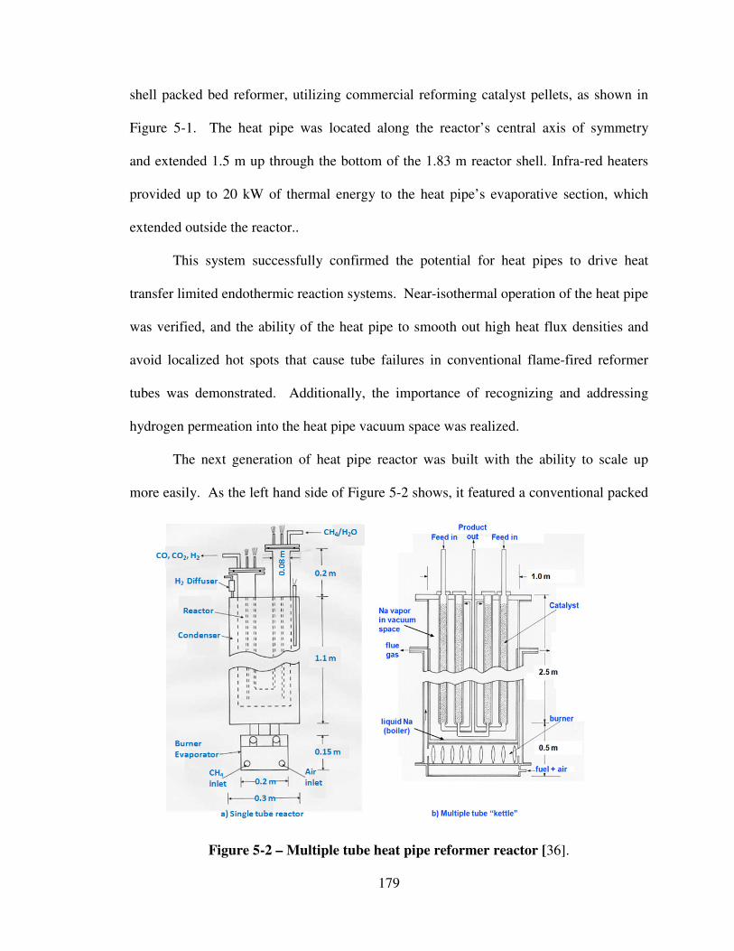
179
shell packed bed reformer, utilizing commercial reforming catalyst pellets, as shown in
Figure 5-1. The heat pipe was located along the reactor’s central axis of symmetry
and extended 1.5 m up through the bottom of the 1.83 m reactor shell. Infra-red heaters
provided up to 20 kW of thermal energy to the heat pipe’s evaporative section, which
extended outside the reactor..
This system successfully confirmed the potential for heat pipes to drive heat
transfer limited endothermic reaction systems. Near-isothermal operation of the heat pipe
was verified, and the ability of the heat pipe to smooth out high heat flux densities and
avoid localized hot spots that cause tube failures in conventional flame-fired reformer
tubes was demonstrated. Additionally, the importance of recognizing and addressing
hydrogen permeation into the heat pipe vacuum space was realized.
The next generation of heat pipe reactor was built with the ability to scale up
more easily. As the left hand side of Figure 5-2 shows, it featured a conventional packed
Figure 5-2 – Multiple tube heat pipe reformer reactor [36].

180
bed reformer U-tube within a vacuum chamber with sodium vapor as the heat transfer
working fluid. A natural gas burner provided heat to the liquid sodium boiler, generating
sodium vapor. The sodium vapor carried the thermal energy from the burner to the
reformer tube, where it condensed like the condensing zone of a heat pipe and gave up its
latent heat of vaporization to the reforming catalyst inside the tube. With an
appropriately-sized burner unit, such a system could easily be scaled up and expanded to
contain multiple reformer tubes in a “kettle” arrangement as shown in the right side of
Figure 5-2. Such a “kettle” arrangement with a vacuum space is less costly to operate
and maintain than individual heat pipe reactors like those in Figure 5-1. Also, the design
included a palladium or nickel plug in the shell that provided an exit via diffusion
through the metal for hydrogen that passed through the heat pipe wall. This unit operated
at a higher energy level and provided useful operating data for heat pipe driven reformers
than the unit in Figure 5-1.
Based on this experience, a solar driven reformer was designed and built at Sandia
National Laboratories and tested in Israel through a joint Sandia/UH/Weizmann Institute
project [48,70]. This unit operated for 3 to 4 months and demonstrated the ease of
control and startup of solar operation.
This research proved that a heat pipe reforming reactor was viable, and able to
realize the benefits of (1) isothermal operation, (2) self-correcting flux absorption, (3)
easy control, and (4) rapid start-up. These are all beneficial features that improve
operability and reliability, as well as compactness of design versus conventional flame-
fired reforming systems.

181
5.3 Ceramic foam catalyst support selection
Section 2.3 demonstrated how ceramic foam catalyst supports offer improved
mass transfer, heat transfer, and pressure drop characteristics over conventional packed
bed pellet catalyst supports. Based on these earlier results, a ceramic foam with a pore
size rating of 30 PPI (pores per inch) is recommended for this system.
5.4 Reformer and combustor combinations
Figures 5-3 and 5-4 show different options for a steam methane reformer. Figure
5-3 (a) depicts a system which uses a flame-fired gas burner to drive a sodium heat pipe,
which in turn supplies the heat for steam methane reforming. An upgrade to Figure 5-3
(a) is shown in 5-3 (b) in which the gas burner is replaced with a short, large diameter
catalytic combustor. However, this configuration for a catalytic combustor is difficult to
construct, with its annular catalyst bed. It also has limited heat transfer area with the heat
pipe, with only its inner surface in contact with the heat pipe. The outer surface of the
combustor catalyst is not in contact with any working part of the heat pipe, and would
have to be well-insulated to minimize heat losses.
Figure 5-4 (a) is a further refinement of the concentric reformer/combustor
concept, and features a full length concentric catalytic combustor to overcome any
limitation of heat transfer area with the heat pipe. Unfortunately, it still is a difficult
design to construct, with its concentric catalytic combustor bed. On the other hand, an
end to end design like in Figure 5-4 (b) can be more easily constructed, since both
reformer and combustor catalyst beds are cylindrical and mounted end to end, separated
by a divider wall. The combustor is completely surrounded by the heat pipe, so thermal
losses from the combustor can easily be minimized. Feed and product connections are

182
Figure 5-3 – Reformers driven by (a) gas, or (b) catalytic combustion.
Figure 5-4 – Reformer/Combustor combinations (a) concentric, or (b) end to end.

183
readily accessible. Another advantage of the design of Figure 5-4 (b) is that auxiliary
heaters for startup are easily mounted to the lower end of the heat pipe. That is not
possible with the designs of Figure 5-3 (b) or 5-4 (a).
Based on the advantages of easier construction, less thermal energy loss, and ease
of startup, the optimal configuration for a coupled reformer/combustor system is the end
to end system as depicted in Figure 5-4(b).
5.5 Summary and recommended configuration
The goal of the preceding studies has been to produce a design tool for small
hydrogen plants that builds upon the technological foundations already established at the
University of Houston in the areas of (1) ceramic foam combustor catalyst supports, (2)
heat pipe reactors, and (3) ceramic foam reformer catalyst supports. This current study
has added to that body of knowledge with the development of a computer design model
that is (1) operable on any personal computer without special software, (2) proven valid
for predicting the heat transfer behavior of ceramic foam reactors, and (3) proven valid
for predicting the kinetic response of combustion and reforming of ceramic foam
reactions. Perhaps the most significant contribution of this work which helped the
computer model “dial-in” its heat transfer predictive capabilities, was described in section
3.6.1 (Model upgrades). In this section, parametric evaluation provided a path leading to
discovery of a parameter modification that solved a longstanding heat transfer issue at the
reactor wall. These developments raise the confidence level for using the computer
model in designing a working system, which is the next step.
The best reformer and combustor configuration is an end to end arrangement with
an annular external heat pipe, as in Figure 5-4(b). The catalyst beds for both the reformer

184
and the combustor are cylindrical, which are easier to fabricate and install. Such an
arrangement also allows unhindered installation of a startup heater to the external surface
of the heat pipe so that rapid startup, a desirable trait for reforming systems, is possible.
5.5.1 Sizing basis – Recall from section 4.1.1 when discussing the basis of design
for a small hydrogen plant, that a production capacity of 500 kg/day of hydrogen would
adequately supply a small residential-area filling station. Recall also that this would be
split into twelve parallel systems to provide redundancy, and to enable twelve smaller
reactors to be built instead of one large reactor for ease of construction and installation.
The theoretical enthalpy required by the reforming reaction (Equation 2-1) for one of
these small reactors was determined to be 15.5 kW.
5.5.2 Combustor – Due to additional thermal loads and losses determined in
section 4.1.1 (Combustor heat output), the designed thermal output of the combustor had
to be raised from the theoretical 15.5 kW up to 31 kW. Of this 31 kW, only 15.5 kW is
transmitted to the heat pipe for reforming. The combustor required to generate this heat
load has a diameter of 15.24 cm (6 inches) and a length of 100 cm (39 inches). It takes a
feed of 51.8 SLPM of methane, and 1,694 SLPM of air.
The conversion profile of a combustor operating at these design parameters was
originally presented as Figure 4-3, and is reproduced here. It shows that conversion goes
to completion at a z* distance of 0.14 (14 cm), leaving the remaining 86% of the length
of the combustor available to transfer heat to the heat pipe.
The axial temperature profile and delta wall temperature for the combustor was
also presented previously (Figure 4-2). It is reproduced here, for reference, and it shows

185
Figure 4-3 – Axial conversion profile for combustor.
Figure 4-2 Average axial temperature for the long (100 cm) combustor.
how the average axial temperature peak of 1,100ºC occurs at the same point that
conversion goes to completion, then decays through the bed, eventually dropping to
822ºC at the combustor exit. A significant aspect of Figure 4-2 is that the delta wall-
temperature is positive starting at a z* distance of 0.06 (6 cm), and stays positive for the
rest of the combustor’s length. This illustrates that the combustor passes thermal energy

186
to the heat pipe for 94% of the combustor’s length.
It must be mentioned that the average axial temperature does not show the
localized peak temperature that is reached in the bed. For this reactor, examination of the
temperature table from the computer model shows that it has a localized peak
temperature of 1,423ºC at a z* distance of 0.14. From the analysis in section 4.1.3
(emissions), this results in a NOx emission of 3.9 ppmvw during operation, with an
annual NOx emission of 113 lbs/year for all twelve reactors combined.
Another view of combustor performance is a plot of the radial temperature
profiles of the bed. Figure 5-5 shows the radial temperature profiles at six different z*
distances down the bed. Except for the inlet, the profiles at the other five z* distances are
all above the heat pipe temperature of 800ºC, indicating that the combustor is giving
energy to the heat pipe.
Figure 5-5 – Radial temperature profile versus z* distance for the combustor.
5.5.3 Reformer - The hydrogen production design basis for the reformer reactor
is one twelfth of 500 kg/day, which calculates to an energy demand of 15.5 kW. This
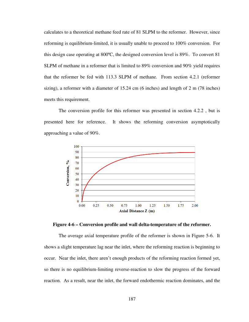
187
calculates to a theoretical methane feed rate of 81 SLPM to the reformer. However, since
reforming is equilibrium-limited, it is usually unable to proceed to 100% conversion. For
this design case operating at 800ºC, the designed conversion level is 89%. To convert 81
SLPM of methane in a reformer that is limited to 89% conversion and 90% yield requires
that the reformer be fed with 113.3 SLPM of methane. From section 4.2.1 (reformer
sizing), a reformer with a diameter of 15.24 cm (6 inches) and length of 2 m (78 inches)
meets this requirement.
The conversion profile for this reformer was presented in section 4.2.2 , but is
presented here for reference. It shows the reforming conversion asymptotically
approaching a value of 90%.
Figure 4-6 – Conversion profile and wall delta-temperature of the reformer.
The average axial temperature profile of the reformer is shown in Figure 5-6. It
shows a slight temperature lag near the inlet, where the reforming reaction is beginning to
occur. Near the inlet, there aren’t enough products of the reforming reaction formed yet,
so there is no equilibrium-limiting reverse-reaction to slow the progress of the forward
reaction. As a result, near the inlet, the forward endothermic reaction dominates, and the

188
temperature has a slight lag. As reforming reaction products accumulate, then the reverse
reaction becomes significant, and begins to hinder the forward reaction. Hence, the bed
temperature begins rising for the rest of the length of the reactor, as seen in Figure 5-6.
Figure 5-6 – Average axial temperature profile versus z* distance for the reformer.
The radial temperature profiles of the reformer reactor at various distances down
the reactor bed are shown in Figure 5-7. It shows that the centerline core temperature
always lags behind the wall temperature, which is being held at 800ºC by the heat pipe.
Therefore, thermal energy is always flowing from the heat pipe, into the reformer.
Figure 5-7 – Radial temperature profile versus z* distance for the reformer.
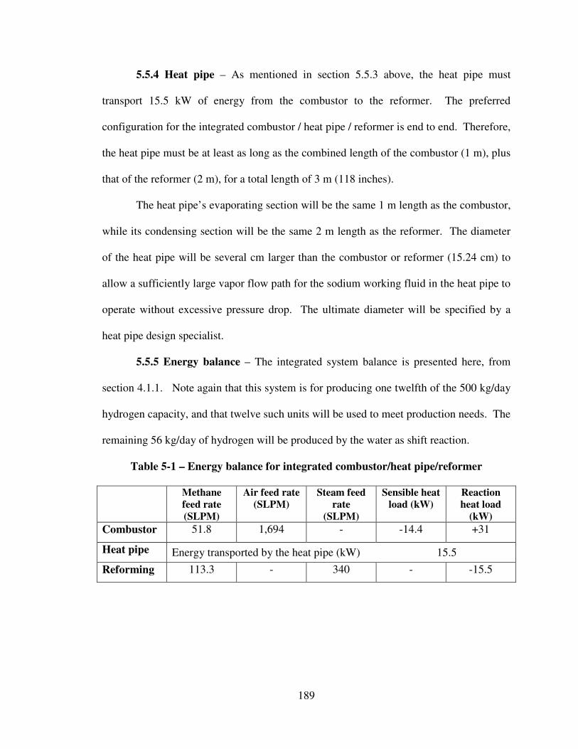
189
5.5.4 Heat pipe – As mentioned in section 5.5.3 above, the heat pipe must
transport 15.5 kW of energy from the combustor to the reformer. The preferred
configuration for the integrated combustor / heat pipe / reformer is end to end. Therefore,
the heat pipe must be at least as long as the combined length of the combustor (1 m), plus
that of the reformer (2 m), for a total length of 3 m (118 inches).
The heat pipe’s evaporating section will be the same 1 m length as the combustor,
while its condensing section will be the same 2 m length as the reformer. The diameter
of the heat pipe will be several cm larger than the combustor or reformer (15.24 cm) to
allow a sufficiently large vapor flow path for the sodium working fluid in the heat pipe to
operate without excessive pressure drop. The ultimate diameter will be specified by a
heat pipe design specialist.
5.5.5 Energy balance – The integrated system balance is presented here, from
section 4.1.1. Note again that this system is for producing one twelfth of the 500 kg/day
hydrogen capacity, and that twelve such units will be used to meet production needs. The
remaining 56 kg/day of hydrogen will be produced by the water as shift reaction.
Table 5-1 – Energy balance for integrated combustor/heat pipe/reformer
Methane
feed rate
(SLPM)
Air feed rate
(SLPM)
Steam feed
rate
(SLPM)
Sensible heat
load (kW)
Reaction
heat load
(kW)
Combustor 51.8 1,694 - -14.4 +31
Heat pipe Energy transported by the heat pipe (kW) 15.5
Reforming 113.3 - 340 - -15.5

190
5.5.6 Safety considerations in design – Safety considerations for the major
system components are incorporated as follows;
(1) Catalytic combustor – the air to fuel ratio in the feed to the catalytic combustor is kept
at a minimum of 32.7 to 1, equivalent to a 3 volume% methane in air mixture. This is
well below methane’s lower flammability limit in air of 5 volume%, and will prevent
flammable vapor clouds from forming in the event of a major gas leak in the combustor
feed system.
(2) Sodium vapor heat pipe – The sodium vapor heat pipe is not expected to add
additional hazards to the operation of the integrated reformer system. In the evaporating
zone of the heat pipe connected to the catalytic combustor, the air, methane, and CO2
present in the combustor are at higher pressures than the sodium within the heat pipe, and
can be expected to flow into the heat pipe in case of a wall rupture. However, the
chemical components of the combustor are all compatible with sodium, and no
significant reaction is expected.
In the condensing zone of the heat connected to the reformer, the steam, methane,
carbon monoxide, and hydrogen are all at higher pressures than the sodium vapor in the
heat pipe, and can be expected to flow into the heat pipe in case of a wall rupture.
However, as discussed previously in section 2.8.4, the ingress of steam into the heat pipe
in this scenario is rapidly mitigated by pressure buildup from Reactions 2-12 through 2-
14 until the internal pressure balances the external pressure. This occurs rapidly enough
to effectively limit the extent of reaction to less than 10% of the heat pipe sodium
inventory, preventing further pressure buildup [46,47].
191
(3) Catalytic reformer – The reformer processes a feed stream of 25 volume% methane
and 75 volume% steam at elevated pressure to produce hydrogen and carbon monoxide.
The operating pressure is above atmospheric, so ingress of air into the system is not
possible. Within the confines of the piping and reactors in the absence of air, this
reaction system is non-flammable at all compositions so that runaway reactions and
explosions within the equipment are not possible.
In the event of piping leaks, the reforming system poses a risk of releasing
flammable vapors to the atmosphere, similar to conventional steam methane reforming
technology. However, heat pipe reactors with isothermal condensing conditions of
800°C at the reformer wall offer less severe thermal stress compared to conventional
flame-fired reformer wall conditions of over 1,500°C (Figure 2-32). Therefore, reformer
reactor reliability can be expected to be superior for the new technology, reducing the
risk of a reactor rupture and release of flammable vapors..
192
CHAPTER SIX
Integrated steam methane reformer hydrogen plants
6.1 Introduction
The aim of the small scale hydrogen production plant in this study is to provide a
viable, economical alternative source for transportation fuel, or for other small industrial
uses.
6.1.1 Performance targets - To be viable, the hydrogen from this system must be
widely available, at a cost that is competitive with incumbent transportation fuels. There
are two targets which the hydrogen production system must meet: First, since a kilogram
of hydrogen is roughly equivalent in fuel value to a gallon of gasoline, the US.
Department of Energy in 2005 decreed the system must produce hydrogen at a cost
competitive to gasoline at approximately $3/kg, based on pre-tax fuel costs at that time
[84]. An appropriate price for 2012 would be closer to $4/kg, which may increase even
more in the future. Second, for a small neighborhood fueling station, the daily
production volume should initially be 500 kg/day of hydrogen, i.e., 25 to 35 fuel cell
vehicles/day. Later, with further implementation, this number will increase by a factor of
4 to 5.
6.1.2 Integrated flow sheet - The hydrogen production system begins with the
reformer and combustion reactor. The remainder of the plant comprises: (1) compressors
to drive the gas flow through the system, (2) heat exchangers to recover energy otherwise
lost to cooling water or to the air, (3) purification equipment to de-sulfurize the methane
feed, and (4) a separator unit for the hydrogen exiting the reformer to lower CO content
below five parts per million.
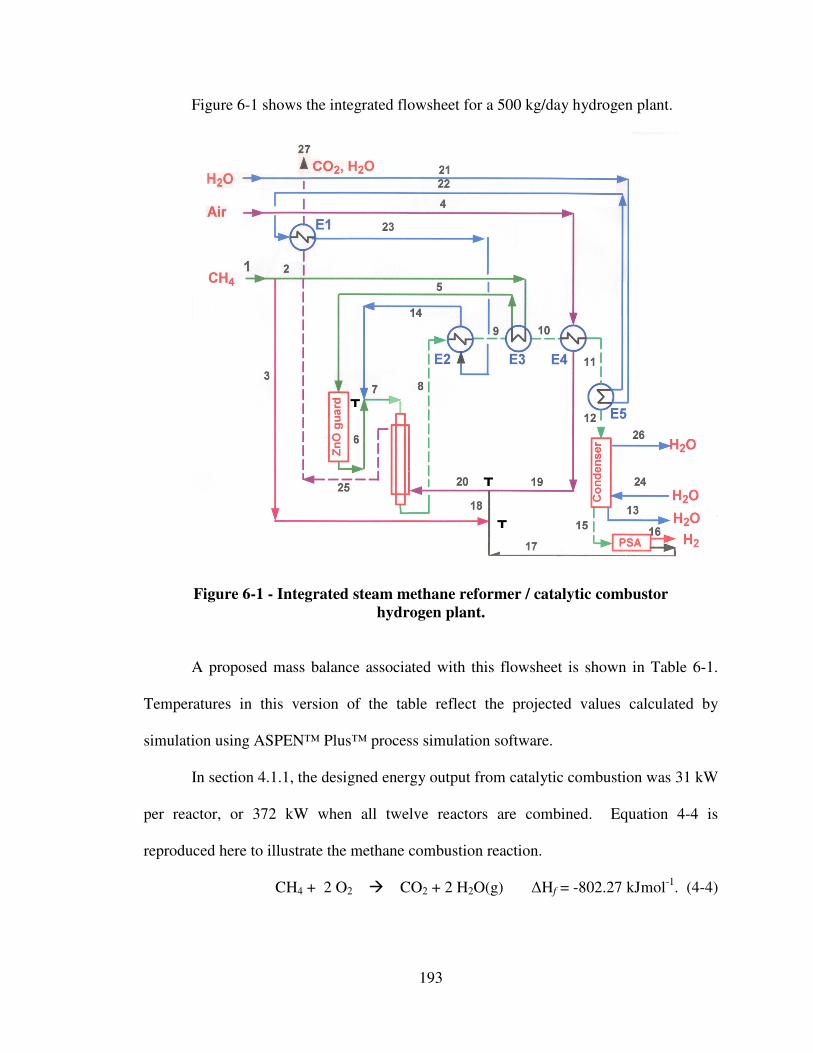
193
Figure 6-1 shows the integrated flowsheet for a 500 kg/day hydrogen plant.
Figure 6-1 - Integrated steam methane reformer / catalytic combustor
hydrogen plant.
A proposed mass balance associated with this flowsheet is shown in Table 6-1.
Temperatures in this version of the table reflect the projected values calculated by
simulation using ASPEN™ Plus™ process simulation software.
In section 4.1.1, the designed energy output from catalytic combustion was 31 kW
per reactor, or 372 kW when all twelve reactors are combined. Equation 4-4 is
reproduced here to illustrate the methane combustion reaction.
CH4 + 2 O2 � CO2 + 2 H2O(g) ∆Hf = -802.27 kJmol-1
. (4-4)
T
T
T

194
The methane flow required to produce 372 kW is 12 × 51.8 SLPM = 622 SLPM, or 1,666
moles/hr.
However, the combustor in the integrated system of Figure 6-1 not only processes
fresh CH4 from stream 3, it also receives fuel from stream 17, consisting of unreacted
recycled CH4, H2 and CO from the PSA. These additional combustion reactions are:
2 H2 + O2 � 2 H2O(g) ∆Hf = -239.93 kJmol-1
, (6-1)
2 CO + O2 � 2 CO2 ∆Hf = -303.06 kJmol-1
. (6-2)
Therefore, instead of using 1,666 moles/hr of just methane in the combustors as
calculated in section 4.1.1, the equivalent energy is provided in stream 20 in Table 6-1
by; (1) 219 moles/hr of recycled unreacted CH4 from the PSA, (2) 2,117 moles/hr of CO
rejected by the PSA, (3) 1,158 moles/hr H2 rejected by the PSA, and (4) 294 moles/hr of
fresh makeup CH4 from stream 3.
6.1.3 Heat balance - Heat duties of each heat exchanger were evaluated and
adjusted until all were thermodynamically consistent using ASPEN™ PLUS™, version
7.1. A screen view of the ASPEN™ steady state model configuration showing all the
components is shown in Figure 6-2. From the ASPEN™ model runs, the optimized heat
duty for each heat exchanger was established, and is shown in Figure 6-3. It shows the
hot side and cold side duties in kJ/hr for all the heat exchangers in the process. The hot
side duty (in red) is equal to the cold side duty (in blue) for each exchanger because the
process simulation model did not factor in any energy lost to the environment.

195
Table 6-1 - Mass balance for the steam methane reformer / catalytic combustor
hydrogen plant of Figure 6-1
TEMP CH4 H2O CO H2 CO2 N2 O2 PRES
STREAM (o C) Mole/hr Mole/hr Mole/hr Mole/hr Mole/hr Mole/hr Mole/hr (atm)
1 25 3936 0 0 0 0 0 0 6.50
2 25 3641 0 0 0 0 0 0 6.50
3 25 294 0 0 0 0 0 0 1.50
4 25 0 0 0 0 0 11882 3196 2.13
5 351 3641 0 0 0 0 0 0 5.75
6 351 3641 0 0 0 0 0 0 5.00
7 532 3641 10924 0 0 0 0 0 5.00
8 800 219 6196 2117 11574 1307 0 0 3.88
9 595 219 6196 2117 11574 1307 0 0 3.25
10 523 219 6196 2117 11574 1307 0 0 2.50
11 523 219 6196 2117 11574 1307 0 0 1.75
12 97 219 6196 2117 11574 1307 0 0 1.00
13 35 0 6196 0 0 0 0 0 1.00
14 623 0 10924 0 0 0 0 0 5.00
15 35 219 0 2117 11574 1307 0 0 1.00
16 37 0 0 0 10417 0 0 0 1.00
17 37 219 0 2117 1158 1307 0 0 1.50
18 27 513 0 2117 1158 1307 0 0 1.50
19 25 0 0 0 0 0 11882 3196 1.50
20 16 513 0 2124 1158 1307 11882 3196 1.25
21 95 0 10924 0 0 0 0 0 7.25
22 167 0 10924 0 0 0 0 0 6.50
23 249 0 10924 0 0 0 0 0 5.75
24 25 0 527369 0 0 0 0 0 1.00
25 823 0 2185 0 0 3937 11882 532 1.50
26 45 0 527369 0 0 0 0 0 1.00
27 169 0 2185 0 0 3937 11882 532 1.25
Closing the energy balance requires a slight modification of the temperature
profile to ensure thermodynamic consistency (Table 6-2). The red highlighted fields in
Table 6-2 signify that these heat exchangers have approach temperatures, defined as
Tapproach = THot,out-TCold,out , (6-3)
which are negative, and require special design consideration, such as multi-shell design.
For those heat exchangers with a negative temperature approach, a graphical
method of determining the number of shells required is similar to the McCabe-Thiele of
determining the number of stages in a distillation column. Starting with a graphical plot
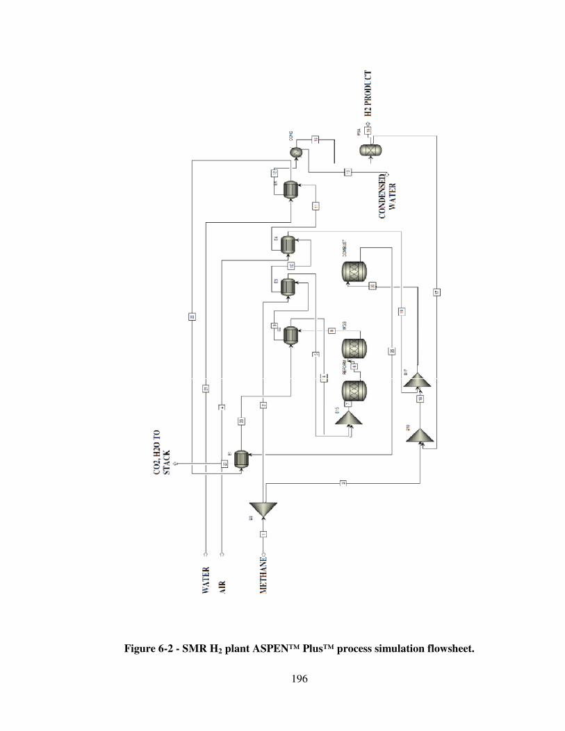
196
Figure 6-2 - SMR H2 plant ASPEN™ Plus™ process simulation flowsheet.

197
Figure 6-3 - SMR H2 plant heat duty by heat exchanger.
Table 6-2 –Temperatures for the integrated H2 plant
E1 E2 E3 E4 E5 CONDENSER
Hot In 823 800 595 523 522 419
Hot Out 169 595 523 522 419 35
Cold Out 250 623 351 25 168 45
Cold In 168 250 25 25 95 25
Approach -81 -28 172 497 251 -10
of the hot fluid and cold fluid temperatures, as in Figure 6-4, draw a horizontal line from
the cold side outlet towards the right until it touches the hot side fluid path. Drop a
vertical line back to the cold side path. Draw another horizontal line to the right to the
hot side path and then drop a vertical line back to the cold side path. Repeat until the
right side end is reached. The total number of times the horizontal lines touch the hot
side path plus one is the number of shells required for that heat duty. In the case of E-1
in Figure 6-4, the number of shells required is three. This is more apparent if the scale is
expanded toward the right hand side of Figure 6-4 as shown in Figure 6-5. The same
analysis performed on E-2 and the condenser yields a shell count of two for each.
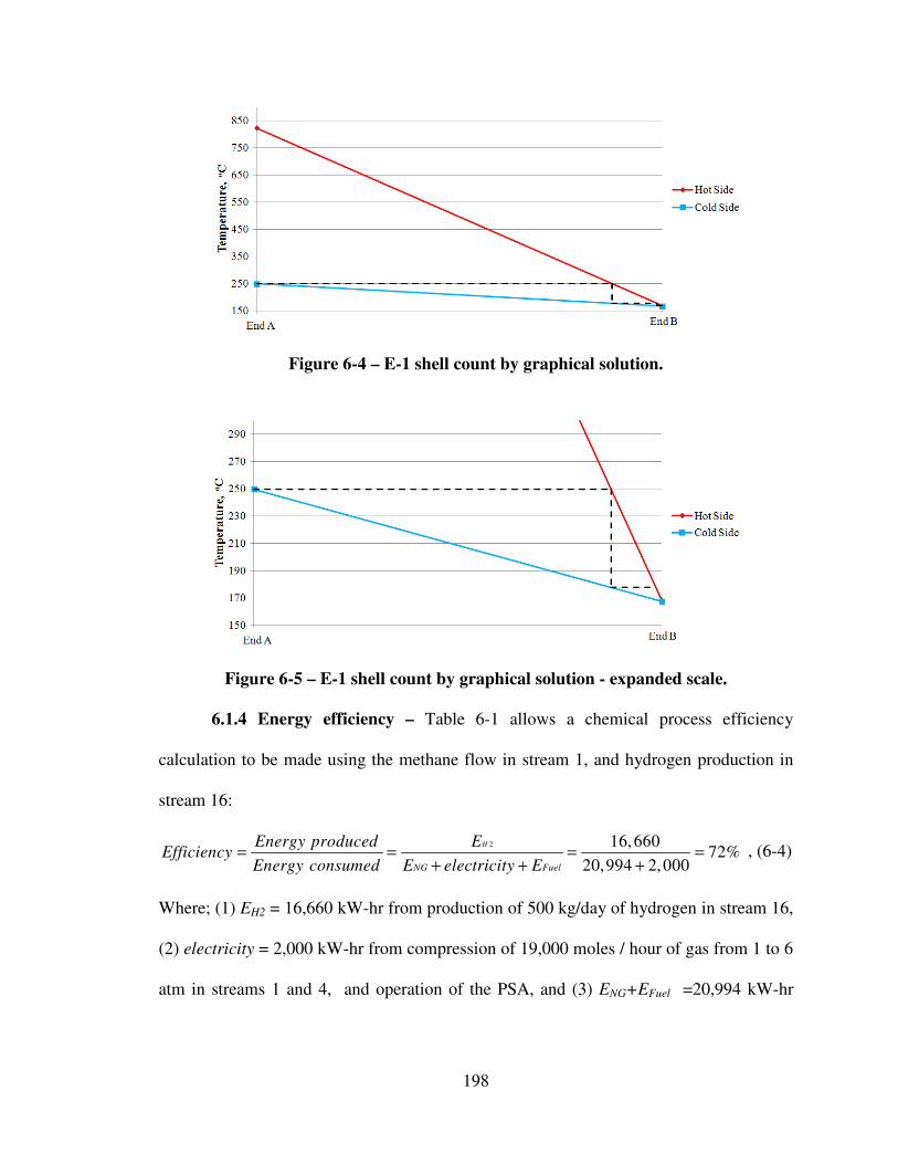
198
Figure 6-4 – E-1 shell count by graphical solution.
Figure 6-5 – E-1 shell count by graphical solution - expanded scale.
6.1.4 Energy efficiency – Table 6-1 allows a chemical process efficiency
calculation to be made using the methane flow in stream 1, and hydrogen production in
stream 16:
2 16,66072%
20,994 2,000
H
NG Fuel
Energy produced EEfficiency
Energy consumed E electricity E= = = =
+ + +
, (6-4)
Where; (1) EH2 = 16,660 kW-hr from production of 500 kg/day of hydrogen in stream 16,
(2) electricity = 2,000 kW-hr from compression of 19,000 moles / hour of gas from 1 to 6
atm in streams 1 and 4, and operation of the PSA, and (3) ENG+EFuel =20,994 kW-hr

199
from natural gas in stream 1. Efficiencies of seventy percent or higher are competitive
with other hydrogen producing technologies.
6.2 System components and estimated costs
The following components are sized based on the 500 kg hydrogen/day, or 20.8
kg hydrogen / hour criteria set in section 6.1.1 above. These figures are for bare
equipment costs only, as installation costs, wiring, controls, and piping are added later.
6.2.1 Reformer and combustor heat-pipe reactor - The reformer and combustor
reactors were modeled together as a 15.24 cm (6 inches) diameter by 3 m (118 inches)
long end to end ceramic foam bed system per Figure 5-4b in section 5.4. Twelve such
reactors are required, and they will each have an external annular concentric sodium
vapor heat pipe. Reactors of this size are possible from shop-built pre-fabricated process
modules that fit within standard box trailers or shipping containers. The compact size of
these reactors combined with modular shop-built construction lower the construction cost
and equipment footprint of these units over conventional reforming systems.
The combustors will process a composite feed of CH4, CO, and H2 per stream 20
in Table 6-1 of 316 moles/hr per reactor, each producing 31 kW of energy. Of this
energy, 15.5 kW will be transported by the heat pipe to the reformer.
The reformers will process 1,214 moles/hr of CH4 and steam each per stream 7 in
Table 6-1. An equilibrium conversion of 89% translates into a daily production rate of
46.3 kg of hydrogen per day per reactor for a gross total of 555 kg/day, before a 10%
yield loss in the hydrogen separation system. The combination reformer/heat pipe
/combustor with dimensions is shown diagrammatically in Figure 6-6. A tube containing

200
a disc of palladium is inserted in the top (not shown) to allow hydrogen diffusing from
the reactor to escape.
The reactor dimensions are approximately 3 m long by 0.3 m in diameter using
the simplified end to end layout from section 5.4. Carbon steel is not a suitable candidate
for the reactor vessels because of high temperature exposure above 1,000ºC at elevated
pressures, as well as attack from hydrogen permeation. Therefore, Inconel™ or other
high temperature alloy steels are required for the reactors. The reformer/heat
pipe/combustor combination in Figure 6-6 is similar in construction to a double pipe heat
exchanger of the same size.
The cost of a 3 m long double pipe heat exchanger of the required pressure rating
(300 psig) built of 304 SS by a heat pipe manufacturer was priced in 2007 dollars at
$3,700 [71], and was adjusted to the latest 2011 CEPCI cost index to $4,147 [72]. The
cost multiplier for Inconel™ over 304 stainless steel of 5.66 [73,74] was applied for a
total rolled up cost of $23,460 per reactor. Twelve reactors will be needed for the full
500 kg/day hydrogen production capacity.
6.2.2 Heat Exchangers - The heat exchangers for the flowsheet in Figure 6-1
were sized using commercial heat exchanger design software by Heat Transfer Research,
Inc. based on the heat load and conditions in Table 6-1. An example output report is
shown in Figure 6-7. Figure 6-7 highlights process conditions, performance, and
configuration of the example heat exchanger evaluation.
Table 6-3 tabulates the sizing results for all six heat exchangers. To price them,
16 actual heat exchanger purchases by a Houston–area chemical plant were used to
develop a cost versus size correlation shown in Figure 6-8.
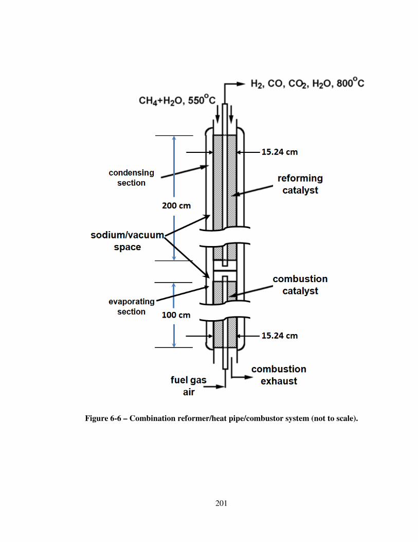
201
Figure 6-6 – Combination reformer/heat pipe/combustor system (not to scale).

202
Figure 6-7 – Heat exchanger evaluation summary page for E-4.

203
Figure 6-8 – Heat exchanger price to size correlation.
Table 6-3 – Heat exchanger sizes and prices
Area
m2 ft
2 2006$ 2011$
E1 112.64 1,212.45 $57,369 $67,623
E2 50.56 544.22 $39,405 $46,449
E3 8.36 89.93 $16,941 $19,969
E4 61.46 661.50 $43,181 $50,899
E5 6.11 65.77 $14,629 $17,244
E6 318.59 3,429.27 $93,412 $110,109
COND 40.97 440.99 $35,704 $42,086
Total $354,380
6.2.3 Hydrogen purification - Literature searches reveal that the cost of a pair of
QuestAir H-3200 pressure-swing adsorption units to produce 500 kg/day of hydrogen is
approximately $415,000 [75].

204
6.2.4 Overall cost of an integrated system - Table 6-4 summarizes the major
equipment costs for the plant. There are additional equipment pieces included that are
available as off the shelf items, such as gas compressors, water pumps, and cooling
systems. The installation markups varied from 1.5 to 3.5 due to the degree of auxiliary
details such as piping, instrumentation required to complete the installation of the
equipment [85]. A modifier to the installation cost factor is a 35% reduction due to
efficiencies realized by in-shop fabrication of the system, as opposed to field construction
[86, 87]. The overall rolled-up cost is $2,286,069 for a 500 kg/day hydrogen plant. This
investment does not include storage or dispensing facilities for the end users, but the cost
of these manufacturing facilities will be compared against other competing technologies.
Table 6-4 - Major equipment costs for SMR H2 plant
Major pieces/systems of
equipment
Baseline 2005
Uninstalled
Costs
Installation
Cost
Factor [85]
Baseline 2009
Installed Costs
Heat Exchangers $ 354,380 3.5×65% $ 937,349
Reactors (12) $ 281,520 3.5×65% $ 744,632
NG Feed compressor $ 12,000 1.5×65% $ 13,603
Air Feed compressor $ 12,500 1.5×65% $ 14,170
Water feed pump $ 10,000 1.5×65% $ 11,336
Refrigeration System $ 83,398 1.5×65% $ 94,539
PSA System $ 415,000 1.5×65% $ 470,439
TOTALS $ 1,168,798 $ 2,286,069
6.2.5 Impact of the experience curve on system cost - It is well known that the
cost to manufacture a product is more expensive when produced in limited numbers early
on in the development. Over time, however, as experience grows and efficiencies
improve, the cost per unit of manufacture decreases as more units are built. The same is
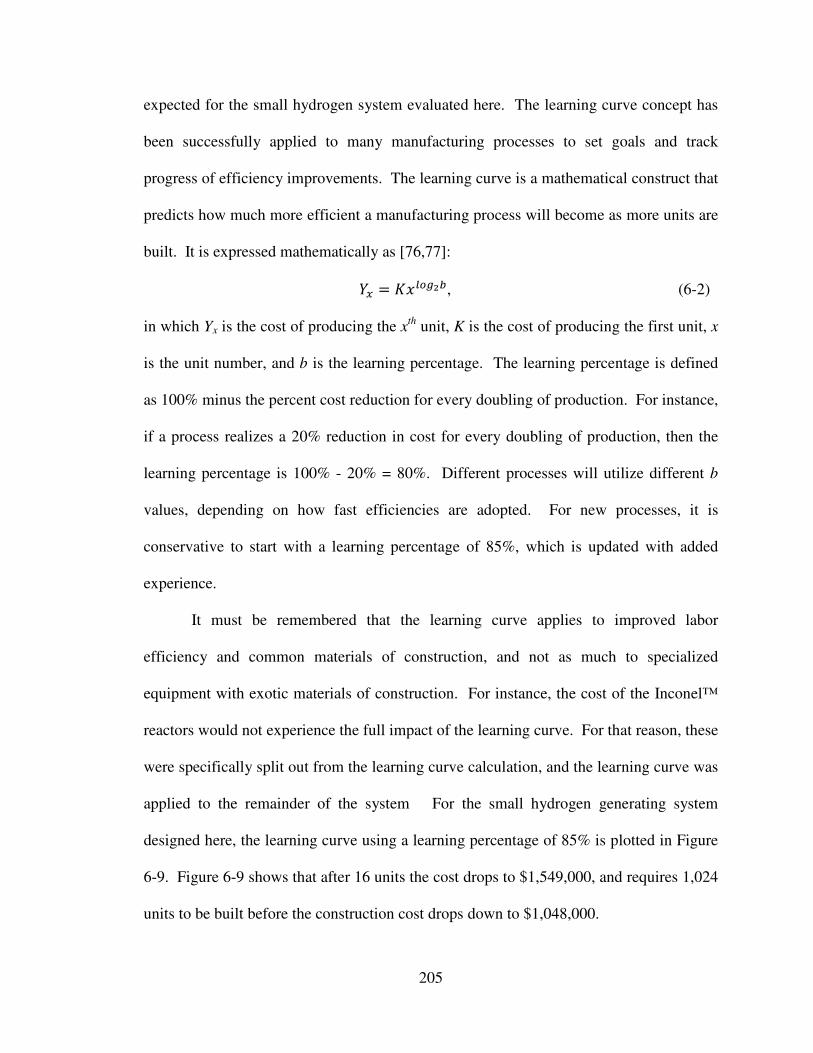
205
expected for the small hydrogen system evaluated here. The learning curve concept has
been successfully applied to many manufacturing processes to set goals and track
progress of efficiency improvements. The learning curve is a mathematical construct that
predicts how much more efficient a manufacturing process will become as more units are
built. It is expressed mathematically as [76,77]:
OP = QRS&TUV, (6-2)
in which Yx is the cost of producing the xth
unit, K is the cost of producing the first unit, x
is the unit number, and b is the learning percentage. The learning percentage is defined
as 100% minus the percent cost reduction for every doubling of production. For instance,
if a process realizes a 20% reduction in cost for every doubling of production, then the
learning percentage is 100% - 20% = 80%. Different processes will utilize different b
values, depending on how fast efficiencies are adopted. For new processes, it is
conservative to start with a learning percentage of 85%, which is updated with added
experience.
It must be remembered that the learning curve applies to improved labor
efficiency and common materials of construction, and not as much to specialized
equipment with exotic materials of construction. For instance, the cost of the Inconel™
reactors would not experience the full impact of the learning curve. For that reason, these
were specifically split out from the learning curve calculation, and the learning curve was
applied to the remainder of the system For the small hydrogen generating system
designed here, the learning curve using a learning percentage of 85% is plotted in Figure
6-9. Figure 6-9 shows that after 16 units the cost drops to $1,549,000, and requires 1,024
units to be built before the construction cost drops down to $1,048,000.
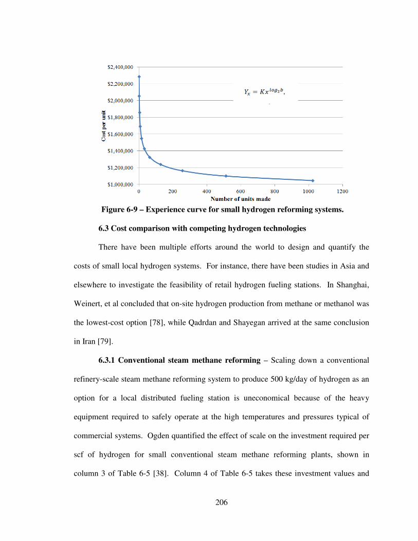
206
Figure 6-9 – Experience curve for small hydrogen reforming systems.
6.3 Cost comparison with competing hydrogen technologies
There have been multiple efforts around the world to design and quantify the
costs of small local hydrogen systems. For instance, there have been studies in Asia and
elsewhere to investigate the feasibility of retail hydrogen fueling stations. In Shanghai,
Weinert, et al concluded that on-site hydrogen production from methane or methanol was
the lowest-cost option [78], while Qadrdan and Shayegan arrived at the same conclusion
in Iran [79].
6.3.1 Conventional steam methane reforming – Scaling down a conventional
refinery-scale steam methane reforming system to produce 500 kg/day of hydrogen as an
option for a local distributed fueling station is uneconomical because of the heavy
equipment required to safely operate at the high temperatures and pressures typical of
commercial systems. Ogden quantified the effect of scale on the investment required per
scf of hydrogen for small conventional steam methane reforming plants, shown in
column 3 of Table 6-5 [38]. Column 4 of Table 6-5 takes these investment values and

207
calculates the equivalent investment versus size of plant, scaled up to 2011 dollars using
chemical plant construction indices [72]. When the investments of Table 6-5 are plotted
in Figure 6-10, the investment for a 500 kg/day conventional reforming plant is equal to
$2.4 million, 5% higher than the investment for the ceramic foam heat pipe reactor
system in Table 6-4. Note that these investment values are for hydrogen production only,
and do not include storage or dispensing equipment.
Table 6-5 – Conventional steam methane reforming plant costs versus scale [38]
Plant capacity Capital
$/kW H2[38]
Plant investment,$
(scf) (kg/day)
100,000 253 $4,000 $2,097,600
1,000,000 2,528 $750 $3,933,000
20,000,000 50,566 $200 $20,975,000
200,000,000 505,658 $80 $83,904,600
Figure 6-10 – Conventional steam methane reforming plant cost versus scale [38].
Weinart, et al., evaluated the total levelized cost of delivered hydrogen for two
different sizes of hydrogen fueling stations in Shanghai, including capital and operating
cost [78]. Table 6-6 shows the investment and cost per kg of hydrogen for these cases. If
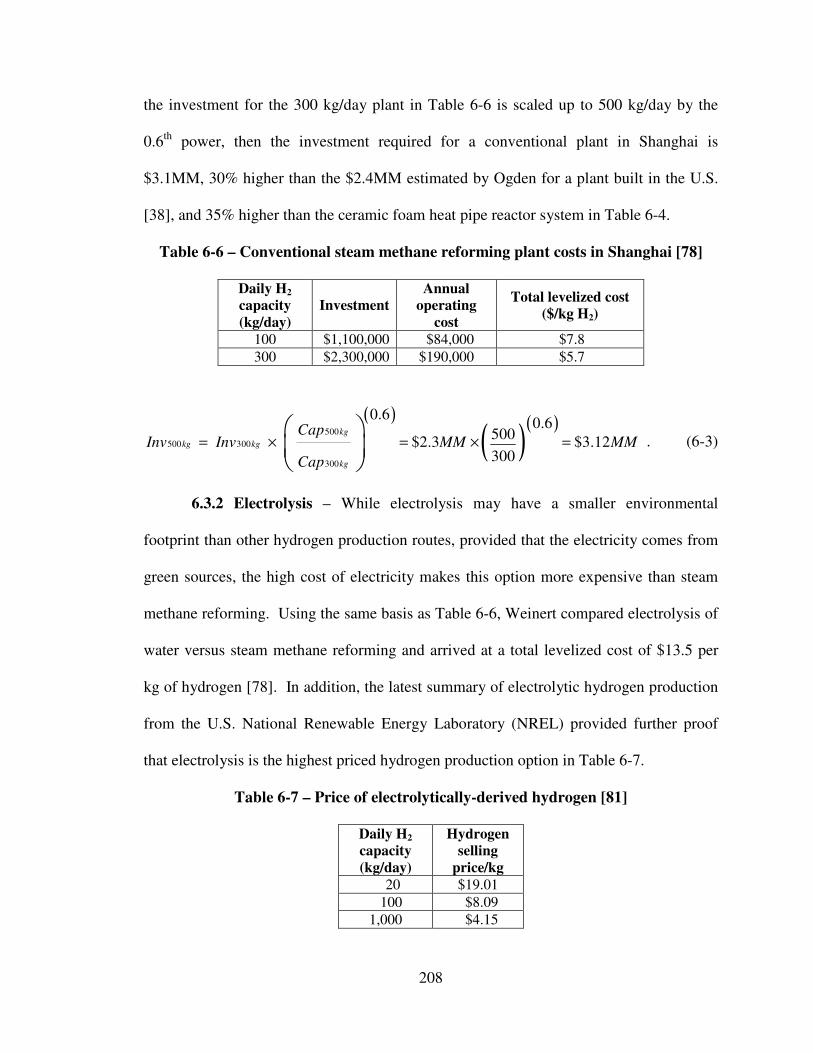
208
the investment for the 300 kg/day plant in Table 6-6 is scaled up to 500 kg/day by the
0.6th
power, then the investment required for a conventional plant in Shanghai is
$3.1MM, 30% higher than the $2.4MM estimated by Ogden for a plant built in the U.S.
[38], and 35% higher than the ceramic foam heat pipe reactor system in Table 6-4.
Table 6-6 – Conventional steam methane reforming plant costs in Shanghai [78]
Daily H2
capacity
(kg/day)
Investment
Annual
operating
cost
Total levelized cost
($/kg H2)
100 $1,100,000 $84,000 $7.8
300 $2,300,000 $190,000 $5.7
( )( )
( )500
500 300
300
0.60.6
500 $2.3 $3.12
300
kg
kg kg
kg
CapInv Inv MM MM
Cap
= × = × =
. (6-3)
6.3.2 Electrolysis – While electrolysis may have a smaller environmental
footprint than other hydrogen production routes, provided that the electricity comes from
green sources, the high cost of electricity makes this option more expensive than steam
methane reforming. Using the same basis as Table 6-6, Weinert compared electrolysis of
water versus steam methane reforming and arrived at a total levelized cost of $13.5 per
kg of hydrogen [78]. In addition, the latest summary of electrolytic hydrogen production
from the U.S. National Renewable Energy Laboratory (NREL) provided further proof
that electrolysis is the highest priced hydrogen production option in Table 6-7.
Table 6-7 – Price of electrolytically-derived hydrogen [81]
Daily H2
capacity
(kg/day)
Hydrogen
selling
price/kg
20 $19.01
100 $8.09
1,000 $4.15

209
6.4 U.S. Department of Energy H2A program
The U.S. Department of Energy sponsored a major development effort to promote
the use of hydrogen energy from 2000 to 2009. They provided an analytical tool to
assess the economic feasibility of various hydrogen energy options called the H2A
program [80]. A prime motivator for this tool was to ensure that different technologies
were assessed using the same economic basis. This tool was used to calculate the
delivered cost of hydrogen for the small hydrogen generating system in this study, from
well to wheels. It evaluates a comprehensive economic analysis of any given hydrogen
supply option, based on the user’s choice of technology, from centralized manufacturing
with truck delivery, to localized electrolysis. The tool requires fairly detailed input
information in order to produce the best analytical result. The basic model architecture
and flow of information is depicted in a pictogram from the H2A model website, in
Figure 6-10. If certain input data are not available, then default values are offered until
better input data are available. The financial inputs that are used in the model
Figure 6-11 – U.S. DOE H2A model architecture [80].
210
to calculate a total lifecycle cost include internal rate of return (IRR), depreciation rate,
salvage value, staffing, property value, and price escalation, as well as the more
traditional data like raw material costs and investment. The tool can also perform
sensitivity analyses to highlight the major contributions to the economics.
The standard economic assumptions used in all evaluations are listed in their
website as follows: (1) Reference year dollars: 2009, (2) debt versus equity financing:
100% equity, (3) after tax internal rate of return: 10% real, (4) inflation rate: 1.9%, (5)
effective total tax rate: 38.9%, (6) depreciation period and schedule: MACRS, central
plant production: 20 yrs., forecourt production: 7 yrs., delivery components: typically 5
years with a few exceptions, (7) economic analysis period: Central plant production —
40yrs., forecourt production — 20 yrs., delivery components model — 20 yrs, (8)
decommissioning costs are assumed equal to salvage value, and (9) an IRR of 10%.
The tool itself is an Excel™ spreadsheet with built-in price forecast tables from
the Energy Information Administration for commodities like natural gas or coal, if they
are called for in the analysis. Calculations are performed using Excel™ macros that are
initiated by the user. Only a portion of the input fields are shown as an example in Table
6-8. The blue cells in the spreadsheet are calculated by the program, while yellow and
green are informational only. Peach-colored cells are required input cells which affect
the economic model. When using this model, the default values for storage and
dispensing were used, to provide an equivalent basis of comparison between options.
Even though the H2A model was updated in 2012 to version 3, the prices of
energy feedstocks were not updated from previous versions. As a result, the analyses do
not take advantage of recent lower natural gas prices of the past year. As an example,

211
Table 6-9 shows the current natural gas price data, in dollars per mmBtus from the
current version 3 H2A model. They show natural gas prices which were earlier forecast
to rise above $10/ mmBtus in the present year. In reality, however, recent market forces,
including newly-discovered reserves and lower usage in the U.S have resulted in natural
gas prices well below those earlier forecasts. Figure 6-12 shows an 8 month decline of
natural gas futures prices in the U.S., to approximately $2.50 per mmBtus, which has a
significant impact on the economics of steam methane reforming. For the H2A analysis
performed on the current system under study, the forecast future price for natural gas feed
stock for the low natural gas price case was scaled back from the $10/mmBtus to a more
conservative $4/mmBtus.
Table 6-8 – U.S. DOE H2A model portion of input screen
.
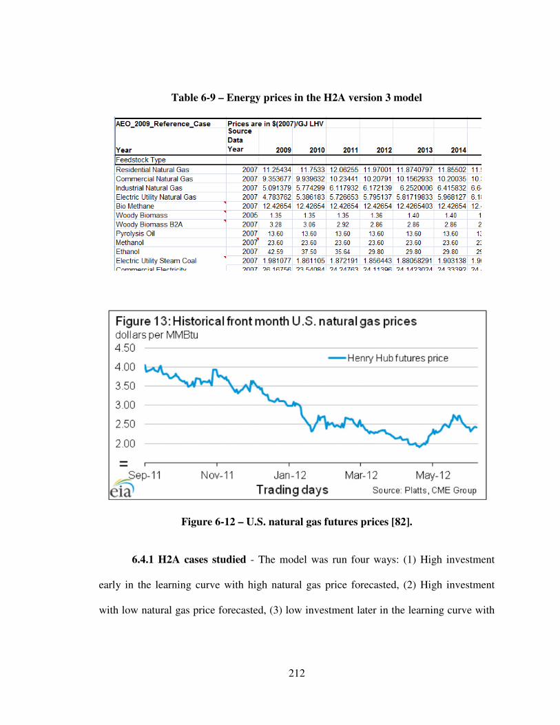
212
Table 6-9 – Energy prices in the H2A version 3 model
Figure 6-12 – U.S. natural gas futures prices [82].
6.4.1 H2A cases studied - The model was run four ways: (1) High investment
early in the learning curve with high natural gas price forecasted, (2) High investment
with low natural gas price forecasted, (3) low investment later in the learning curve with

213
high natural gas price forecasted, and (4) low investment with low natural gas price
forecasted.
6.4.2 High investment high natural gas price case - The H2A model for the
current case was run using these assumptions; (1) a capital investment of $2,286,069
from Table 6-4, (2) the natural gas price forecast as provided in the H2A model, and (3)
the default hydrogen storage and dispensing options. The H2A model yielded a delivered
hydrogen cost of $6.48/kg, as shown in Table 6-10.
Note that for this case, the investment percentage of the hydrogen cost is almost 49%,
and that the feedstock cost is almost 25%.
Table 6-10 – H2A H2 delivered cost for high capital and high natural gas
6.4.3 High investment low natural gas price case - When the natural gas price
forecast is lowered to $4/mmBtus, the hydrogen delivered cost drops 16%, to $5.43/kg,
as shown in Table 6-11. The feedstock as a percent of delivered hydrogen cost drops to
10%, while capital cost as a percentage of delivered hydrogen rises to 58%.
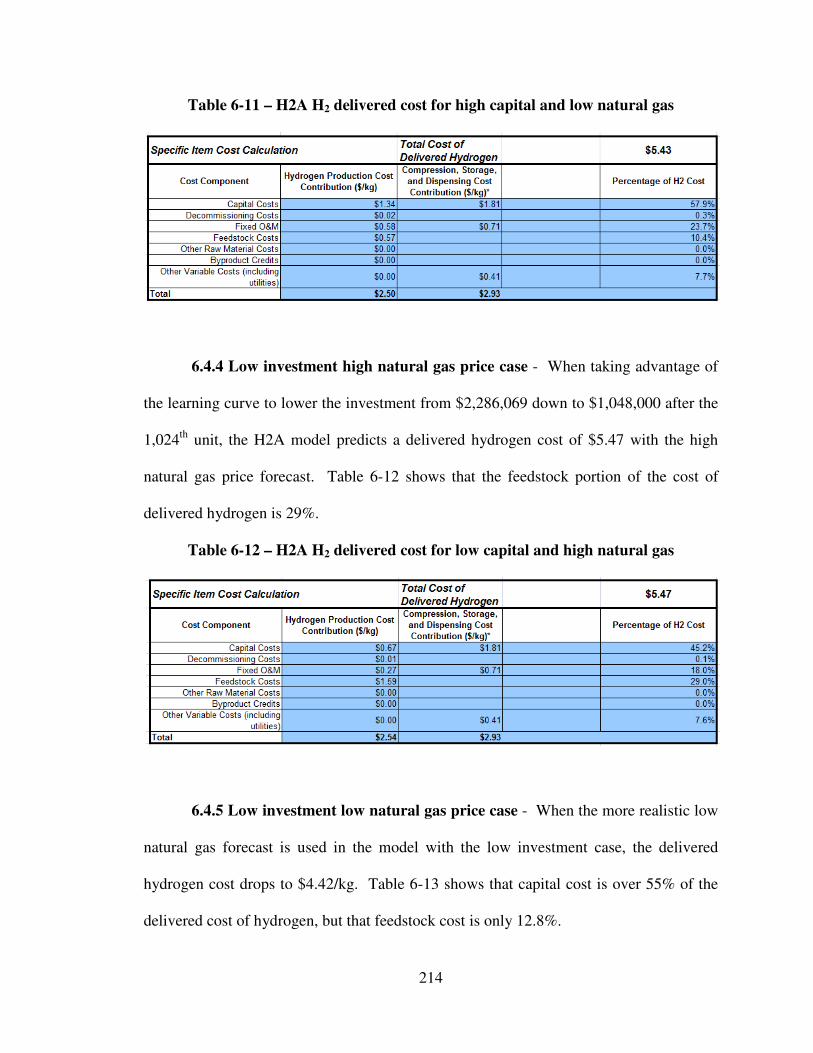
214
Table 6-11 – H2A H2 delivered cost for high capital and low natural gas
6.4.4 Low investment high natural gas price case - When taking advantage of
the learning curve to lower the investment from $2,286,069 down to $1,048,000 after the
1,024th
unit, the H2A model predicts a delivered hydrogen cost of $5.47 with the high
natural gas price forecast. Table 6-12 shows that the feedstock portion of the cost of
delivered hydrogen is 29%.
Table 6-12 – H2A H2 delivered cost for low capital and high natural gas
6.4.5 Low investment low natural gas price case - When the more realistic low
natural gas forecast is used in the model with the low investment case, the delivered
hydrogen cost drops to $4.42/kg. Table 6-13 shows that capital cost is over 55% of the
delivered cost of hydrogen, but that feedstock cost is only 12.8%.

215
Table 6-13 – H2A H2 delivered cost for low capital and low natural gas
6.4.6 Summary of H2A cases - The H2A analysis allows selection of an internal
rate of return (IRR%) when calculating the delivered price of hydrogen. An IRR of 10%
was used in all of the cases up to now, which the program then used to discount all the
cash flows for the 20 year life of the project. The variable that the program uses to
discount all the cash flows so that the NPV is zero is the delivered price of the hydrogen.
That delivered hydrogen price has the 10% IRR built into it.
The four H2A cases are summarized in Table 6-14, and they show that at an IRR
of 10% they are all non-competitive with the current price of gasoline of $3.50/gal. As
gas prices rise, this technology may become competitive again. However, if a lower IRR
Table 6-14 – H2A H2 delivered cost by capital and by natural gas price at 10% IRR
High natural gas Low natural gas
High investment $6.48/kg $5.43/kg
Low investment $5.47/kg $4.42/kg
can be tolerated, the delivered price of hydrogen is lower. For instance, if the IRR were
dropped to 7.5% or 5%, then the delivered hydrogen prices would drop as in Tables 6-15
and 6-16. At an IRR of 5%, the delivered price of hydrogen is in a competitive price
range within reach of today’s gasoline prices at the low investment, low natural gas price
case.
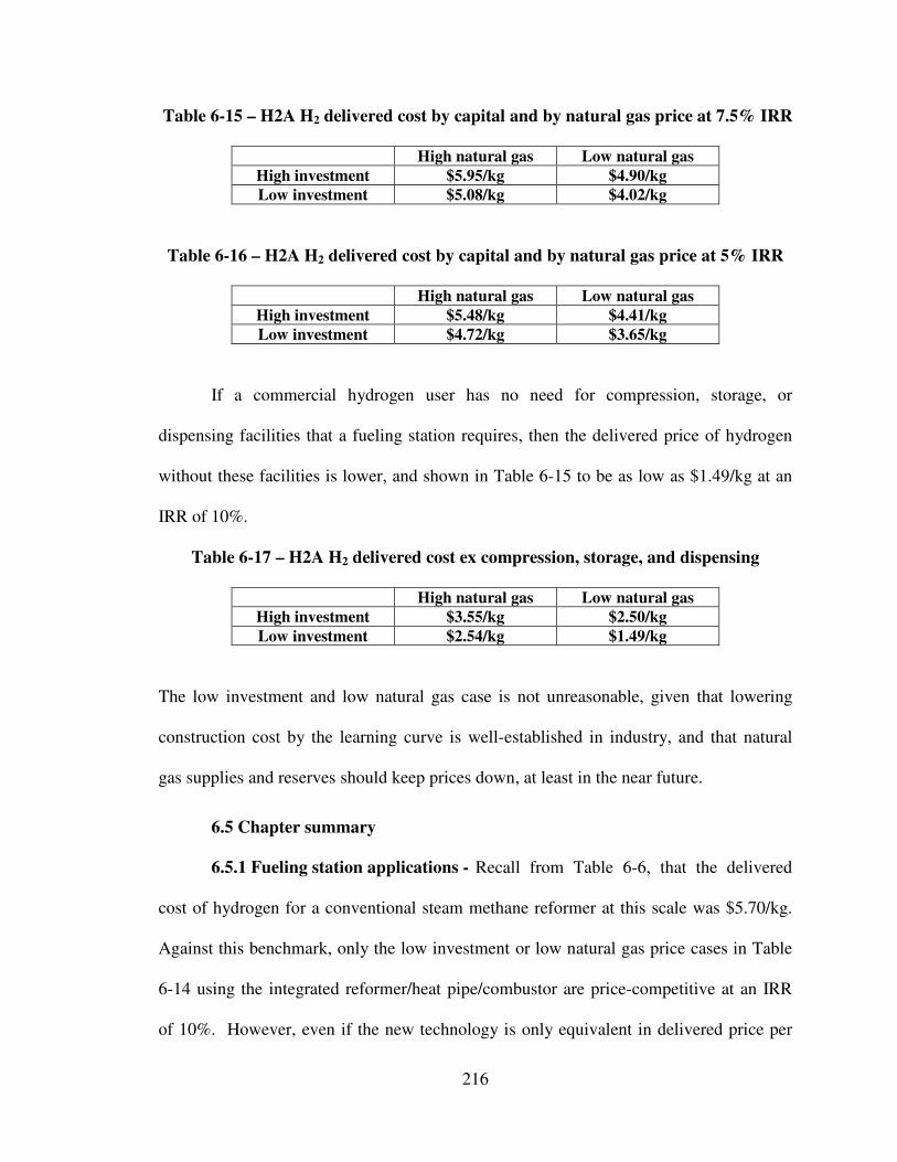
216
Table 6-15 – H2A H2 delivered cost by capital and by natural gas price at 7.5% IRR
High natural gas Low natural gas
High investment $5.95/kg $4.90/kg
Low investment $5.08/kg $4.02/kg
Table 6-16 – H2A H2 delivered cost by capital and by natural gas price at 5% IRR
High natural gas Low natural gas
High investment $5.48/kg $4.41/kg
Low investment $4.72/kg $3.65/kg
If a commercial hydrogen user has no need for compression, storage, or
dispensing facilities that a fueling station requires, then the delivered price of hydrogen
without these facilities is lower, and shown in Table 6-15 to be as low as $1.49/kg at an
IRR of 10%.
Table 6-17 – H2A H2 delivered cost ex compression, storage, and dispensing
High natural gas Low natural gas
High investment $3.55/kg $2.50/kg
Low investment $2.54/kg $1.49/kg
The low investment and low natural gas case is not unreasonable, given that lowering
construction cost by the learning curve is well-established in industry, and that natural
gas supplies and reserves should keep prices down, at least in the near future.
6.5 Chapter summary
6.5.1 Fueling station applications - Recall from Table 6-6, that the delivered
cost of hydrogen for a conventional steam methane reformer at this scale was $5.70/kg.
Against this benchmark, only the low investment or low natural gas price cases in Table
6-14 using the integrated reformer/heat pipe/combustor are price-competitive at an IRR
of 10%. However, even if the new technology is only equivalent in delivered price per
217
kg, additional operating benefits of the integrated system include compact footprint.
faster startup, better operability and easier maintenance with a ceramic foam catalyst bed
than with conventional reformer tubes.
6.5.2 – Small scale applications – Perhaps a more immediate market for the
integrated hydrogen plant is for small hydrogen chemical users and the stationary fuel
power units currently under commercialization. In these cases the costs associated with
compression and delivery shown in Table 6-17 (essentially over 60% of the cost) is not
needed. In addition, purification of the hydrogen is less demanding for many of the
chemical applications and unnecessary for molten carbonate and solid oxide fuel cells.
This makes the delivered cost of $1.49/kg as shown in Table 6-17 very attractive.

218
CHAPTER SEVEN
Conclusions and recommendations
7.1 Conclusions
(1) The 2-D computer model was adapted from existing FORTRAN code for a packed-
bed reactor and successfully updated to better reflect heat transfer in the ceramic foam
bed and at the reactor wall, then validated with experimental heat transfer and reaction
data.
(2) Different configurations and sizes of both reformer and combustor reactors were
studied to arrive at the best configuration for an integrated system, which is an end to end
arrangement of the reformer and combustor. The radial and axial conversion and
temperatures of each reactor were evaluated to match the heat recovery capability of the
reformer to the heat generation characteristics of the combustor.
(3) The vetted computer model was used to size and specify a 500 kg/day hydrogen
production unit featuring ceramic foam catalyst beds integrated into heat pipe reactors
that can be used for multiple end users, ranging from small edible fats and oils
hydrogenators to consumer point of sale hydrogen fueling stations. The estimated
investment for this 500 kg/day system is $2,286,069, but is expected to drop to less than
$1,048,000 using mass production methods.
(4) Economic analysis of the 500 kg/day hydrogen production system shows that at an
IRR of 10%, it is not presently competitive with gasoline as a transportation fuel, but the
system is still economically attractive to stationary fuel cell applications with a delivered

219
hydrogen price as low as $1.49/kg, even with a 10% IRR that includes investment
recovery, depreciation, taxes, etc.
The heat-pipe reformer has been shown to be a superior device for transporting
heat to a highly endothermic reactor, so that reactions such as steam reforming are much
less heat transfer limited. As a result the reforming tube is reduced in length by a factor
of two down to 200 cm. Ceramic foams are structural catalyst supports that exhibit low
pressure drop and radial heat conduction properties that further reduce the length of the
tube and give better stability than traditional particulate catalyst supports.
This system was intended to meet the near-term transitional need for rapid
deployment of distributed hydrogen production facilities in order to foster the growth of
the hydrogen economy. While presently it does not offer a cost advantage over current
petroleum-based fuels, it can be utilized by non-transportation hydrogen users such as
small chemical plants or stationary power fuel-cells to economically meet their hydrogen
needs over electrolysis or truck delivery. However, it must be recognized that no
facilities to capture CO2 are in this scope for small scale hydrogen production, and it is
not believed to be economical at this small a scale.
As the hydrogen economy develops in the future, where CO2 sequestration rises
in importance and large centralized hydrogen plants with hydrogen distribution
infrastructures are created, then the transitional role of small distributed hydrogen
production units such as this will diminish after having paved the way for widespread
acceptance and use of hydrogen energy. However, other methods for small hydrogen
production still exist industrially and compete with this technology for an expanding
market of distributed fuel cell power units.
220
7.2 Recommendations for future work –
The present computer model is separate for both the reformer and the combustor
reactors. It assumes isothermal conditions at the heat pipe interface, at either the
evaporative end (at the combustor), or at the condensing end (at the reformer). An
integrated computer model combining both the reformer and combustor connected by a
dynamic model for the heat pipe would allow more direct evaluation of how they interact
for better prediction of the controllability characteristics of the system.
Each of the elements of the integrated reformer/heat pipe/combustor have been
individually built and demonstrated in the laboratory, but the integrated system in its
entirety has not been constructed. A critical proof test of this concept is to build a
working version, to validate its performance against the model predictions. In addition,
experimental verification of heat transfer correlations and catalytic rate equations should
continue.
The process units not associated with the heat pipe (i.e., heat exchanger,
separation, etc.) are also at reduced scale. Improvements in the design of these
components would have a significant effect on efficiency and costs. For example, the
PSA unit is a major cost factor and is also space consuming. Emerging technology
based on low pressure membranes could play a vital role in reducing costs, and should be
considered as an alternate to PSA. Additionally, micro-channel heat exchangers offer
significant improvements in heat transfer efficiency over traditional shell and tube heat
exchangers.

221
References
1) R. B. Gupta, “Hydrogen fuel; production, transport, and storage,” CRC Press
(2009).
2) U.S. Department of Energy - Energy Efficiency and Renewable Energy, “Fiscal
year 2003 Progress Report,”
http://www1.eere.energy.gov/hydrogenandfuelcells/pdfs/benefits.pdf.
3) U.S. Department of Energy, “The Department of Energy Hydrogen and Fuel Cells
Program Plan,” (2011),
http://www.hydrogen.energy.gov/pdfs/program_plan2011.pdf.
4) U.S. Department of Transportation Research and Innovative Technology
Administration, “Table 2.4. Hydrogen Infrastructure Challenges,” (2008),
http://www.rita.dot.gov/publications/challenges_of_building/html/table_02_04.html
.
5) U.S. Department of Energy, “Distributed Hydrogen Production from Natural gas,”
(2006), http://www.hydrogen.energy.gov/pdfs/40382.pdf.
6) U.S. Department of Energy, “Hydrogen Posture Plan,” (2006),
http://www.hydrogen.energy.gov/pdfs/hydrogen_posture_plan_dec06.pdf.
7) U.S. Department of Energy, Energy Efficiency & Renewable Energy, “Hydrogen
Production,” (2009),
http://www1.eere.energy.gov/hydrogenandfuelcells/production/current_technology.
html.

222
8) P. Ferreira-Aparicio, M. J. Benito, J. L. Sanz, "New Trends in Reforming
Technologies: from Hydrogen Industrial Plants to Multifuel Microreformers,"
Catalysis Reviews 47 (2005): 491–588.
9) N.R. Udengaard, “Hydrogen Production by Steam Reforming of Hydrocarbons,”
ACS division of Fuel Chemistry Advances in Hydrogen Energy Symposium (2004)
Philadelphia, PA.
10) U.S. Census Bureau, “Table 1025. Inorganic Chemicals and Fertilizers –
Production: 2000 to 2009,”
http://www.census.gov/compendia/statab/2011/tables/11s1025.pdf.
11) Pacific Northwest National Laboratory, “Hydrogen Production – Worldwide and
U.S. Total Hydrogen Production,”
http://www.hydrogen.pnl.gov/cocoon/morf/hydrogen/article/706.
12) U.S. Department of Energy, Argonne national Laboratory, “Assessing Current,
Near-term, and Long-term U.S. Hydrogen Markets,”
http://www.dis.anl.gov/news/HydrogenMarkets.html.
13) Argonne National Laboratory, “Overview of Interstate Hydrogen Pipeline
Systems,” ANL/EVS/TM/08-2 (2008),
http://corridoreis.anl.gov/documents/docs/technical/APT_61012_EVS_TM_08_2.p
df.
14) U.S. Department of Energy, Hydrogen Analysis resource Center, “Hydrogen
Pipelines,” http://hydrogen.pnl.gov/cocoon/morf/hydrogen/article/860.
15) U.S. Department of Transportation, Pipeline and hazardous materials Safety
Administration, “General Pipeline FAQs,”

223
http://www.phmsa.dot.gov/portal/site/PHMSA/menuitem.ebdc7a8a7e39f2e55cf2031
050248a0c/?vgnextoid=a62924cc45ea4110VgnVCM1000009ed07898RCRD&vgne
xtchannel=59e9f08df5f3f010VgnVCM1000008355a8c0RCRD&vgnextfmt=print#Q
A_6.
16) C. Yang, J. Ogden, “ Determining the lowest-cost hydrogen delivery mode,” Int. J.
of Hydrogen Energy, 32 (2007) 268-286.
17) U.S. Energy Information Administration, “The Impact of Increased Use of
Hydrogen on Petroleum Consumption and Carbon Dioxide Emissions – Appendix
C,” Report #: SR-OIAF-CNEAF/2008-04 (2008),
http://www.eia.gov/oiaf/servicerpt/hydro/appendixc.html.
18) United States Department of Energy, “National Hydrogen Energy Roadmap,”
National Hydrogen Energy Roadmap Workshop (2002),
http://www.hydrogen.energy.gov/pdfs/national_h2_roadmap.pdf.
19) Research and Innovative Technology Administration, Bureau of Transportation
Statistics, “Table 1-11: Number of U.S. Aircraft, Vehicles, Vessels, and Other
Conveyances,”
http://www.bts.gov/publications/national_transportation_statistics/html/table_01_1
1.html.
20) National Hydrogen Association, “Hydrogen and Fuel Cells: The U.S. Market
Report,” (2010) http://www.ttcorp.com/pdf/marketReport.pdf.
21) National Energy Technology Laboratory, “Backup Generators (BUGS): The Next
Smart Grid Peak resource,” (2010).

224
22) American Iron and Steel Institute, “Suspension Hydrogen Reduction of Iron Oxide
Concentrate,” (2006) http://steeltrp.com/TRPGreenBook2006/9953factsheet.pdf.
23) M.E. Choi, H.Y. Sohn, & G. Han, “Suspension reduction technology for iron
making with low energy requirement and CO2 emission,” Paper presented at the
17th International Metallurgical & Materials Conference, Hradec nad Moravicí,
Czech Republic (2008 May)
http://www.metal2012.com/files/proceedings/metal_08/Lists/Papers/004.pdf.
24) U.S. Department of Energy, “Roadmap on manufacturing R&D for the Hydrogen
Economy,” Draft presented at the Workshop on manufacturing R&D for the
Hydrogen Economy (2005 July),
http://www.hydrogen.energy.gov/pdfs/roadmap_manufacturing_hydrogen_econom
y.pdf.
25) S. Ahmed, M. Krumpelt, R. Kumar, S.H.D. Lee, J.D. Carter, R. Wilkenhoener, and
C. Marshall, “Catalytic Partial Oxidation Reforming of Hydrocarbon Fuels,”
Presentation at the 1998 Fuel Cell Seminar in Palm Springs, California (November
1998), http://www.transportation.anl.gov/pdfs/AF/230.pdf.
26) U.S. Department of Energy - DOE Decision Team Committee report, “On-board
Fuel processing Go/No-go Decision,” (2004)
http://www.hydrogen.energy.gov/pdfs/fuel_processing.pdf.
27) Precision Combustion Incorporated, “Fuel Reformer & Fuel Processing Systems,”
Presentation at the July 15, 2009 U.S. Department of Energy Hydrogen and Fuel
225
Cell Technical Advisory Committee Meeting, North Haven, CT
http://www.hydrogen.energy.gov/pdfs/htac_july09_06_pci.pdf.
28) U.S. Department of Energy – Energy Efficiency and renewable Energy,
“Hydrogen, Fuel Cells & Infrastructure Technologies Program – Multi-Year
Research, Development and Demonstration Plan,” (2009),
http://www1.eere.energy.gov/hydrogenandfuelcells/mypp/
29) U.S. Department of Energy, “Strategic Directions for Hydrogen Delivery,”
Proceedings from the May 7-8, 2003 U.S. Department of Energy Strategic
Initiatives for Hydrogen Delivery Workshop, Arlington, VA,
http://www1.eere.energy.gov/hydrogenandfuelcells/pdfs/h2_delivery_draft_report.p
df.
30) Forsberg, C. W., “Future hydrogen markets for large-scale hydrogen production
systems,” International Journal of Hydrogen Energy 32 (2007) 431 – 439.
31) U.S. Department of Energy, “DOE Hydrogen Program – 2009 Annual Progress
report,” (2009), DOE/GO-102009-2950.
32) G. Thomas, S. Satyapal, “A brief overview of hydrogen storage issues and needs,”
Presentation at the joint meeting on hydrogen delivery modeling and analysis, May
8-9, 2007, Columbia, MD,
http://www1.eere.energy.gov/hydrogenandfuelcells/pdfs/deliv_analysis_thomas.pdf
.
33) G. Mulder, J. Hetland, G. Lenaers, “Towards a sustainable hydrogen economy:
Hydrogen pathways and infrastructure,” International Journal of Hydrogen Energy
32 (2007) 1324 – 1331.
226
34) Sandia National Laboratories, “Autothermal Reforming of Natural gas to Synthesis
Gas,” (2007) SAND2007-2331.
35) D. E. Ridler and M. V. Twigg, “Catalyst Handbook, 2nd. Edition, (M.V. Twigg,
Ed.) Wolfe Publishing Ltd., London (1996).
36) J.T. Richardson, Class Notes for CHEE 6388: Catalytic Processes, University of
Houston.
37) Halder Topsoe, “Steam reforming catalysts,” Product brochure opus 09/01-3,
http://www.topsoe.com/business_areas/hydrogen/Processes/~/media/PDF%20files/
Steam_reforming/Topsoe_steam_reforming_cat.ashx.
38) J. Ogden, “Review of small stationary reformers for hydrogen production,” A
report for the International Energy Agency Agreement on the Production and
Utilization of Hydrogen IEA/H2/TR-02/002(2002),
http://www.afdc.energy.gov/afdc/pdfs/31948.pdf.
39) R. Palluzi, (2010), “Consider modular pilot-plant construction, Retrieved January
15, 2012 from http://www.chemicalprocessing.com/articles/2010/028.html.
40) A. Faghri, “Heat Pipe Science and Technology,” Taylor and Francis, New York
(1995).
41) M.N. Ivanovskii, V. R. Sorokin, I. V. Yagodkin, “The Physical Principles of Heat
Pipes,” Oxford University press, USA (1982).
42) A. Abo El-Nasr, S. M. El-Haggar, “Effective thermal conductivity of heat pipes,”
Heat and Mass Transfer 32 (1996) 97-101.
43) A. J. Chapman, “Heat Transfer – 3rd
edition,” Macmillan Publishing Company,
Inc. New York (1974), 566-571.

227
44) C.A. Busse, “Theory of the ultimate heat transfer limit of cylindrical heat pipes,”
Int. J of Heat Mass Transfer 16 (1973) 163-186.
45) H. Zhang, J. Zhuang, “Research, development and industrial application of heat
pipe technology in China,” Applied Thermal Engineering 23 (2003) 1067-1083.
46) R.S. Reid, J.T. Sena, M. Merrigan, M.G. Elder, A.L. Martinez , “Heat Pipe
Development for Advanced Energy Transport Concepts Phase II Final Report
Covering the Period October 1,1997, to September 30,1998,” Los Alamos
National Library LA-13549-PR.
47) R.S. Reid, T. Sena, A.L. Martinez, “Heat Pipe Development for Advanced Energy
Transport Concepts Final Report Covering the Period January 1999 through
September 2001,” Los Alamos National Library LA-13949-PR.
48) R. B. Diver, J. D. Fish, R. Levitan, M. Levy, E. Meirovitch, H. Rosin, S. A.
Paripatyadar, and J. T. Richardson, "Solar Test of an Integrated Sodium Reflux Heat
Pipe Receiver/ Reactor for Thermochemical Energy Transport," Solar Energy 48
(1992) 21-30.
49) J.T. Richardson, "Novel Heat Pipe Reactor for Improved Reforming," Presentation
at the Spring National AICHE Meeting, Houston, TX, April, 1989.
50) W. M. Robertson, “Hydrogen permeation and diffusion in Inconel 718 and Incoloy
903,” Metallurgical and Materials Transactions A 8 (1977) 1709-1712.
51) J.C. Shen, “Dynamics of a sodium heat pipe natural gas reformer,” Dissertation
(Ph. D.)--University of Houston-University Park, 1984 UH Dissertation 660
1984.S53.

228
52) F.C. Moates, “Intermediate scale studies of a catalytic process for steam reforming
of trichloroethylene,” Dissertation (Ph. D.)--University of Houston-University Park,
1997 UH Dissertation 660 1997.M62.
53) J. T. Richardson, Y. Peng and D. Remue, “Properties of ceramic foam catalyst
supports: pressure drop,” Applied Catalysis A: General, 204 (1), p.19-32, Nov
2000.
54) Y. Peng, “Transport properties of ceramic foam for catalyst support application,”
Dissertation (Ph. D.)--University of Houston-University Park, 2001 UH
Dissertation 660 2001.P46.
55) J.T. Richardson, D. Remue, J.-K. Hung, “Properties of ceramic foam catalyst
supports: mass and heat transfer,” Applied Catalysis A: General 250 (2003) 319–
329.
56) D. Machiraju, “Barium manganese hexaaluminate washcoats on ceramic foams,”
Thesis (M.S.)--University of Houston-University Park, 2003 UH Thesis 660
2003.M32.
57) Y. Peng, J.T. Richardson, “Properties of ceramic foam catalyst supports: one-
dimensional and two-dimensional heat transfer correlations,” Applied Catalysis A:
General 266 (2004) 235–244.
58) O. Cantu, “Improved catalyst for low NOx catalytic combustion,” Dissertation (Ph.
D.)--University of Houston-University Park, 2004 UH Dissertation 660 2004.C365.
59) H. Gadalla, “Graduated loading of catalyst on reticulated ceramic foams,”
Dissertation (Ph. D.)--University of Houston-University Park, 2006 UH
Dissertation 660 2006.G32.

229
60) G,G. Jeba, “A Compact and Efficient Steam Methane Reformer for Hydrogen
Production,” Dissertation (Ph. D.)--University of Houston-University Park, 2010
UH Dissertation 660 2010.J42.
61) M.V.Twigg, J.T.Richardson, “Theory and application of ceramic foam catalysts,”
Trans IChemE 80, Part A (2002) 183-189.
62) P.N. Dwivedi, S.N.Upadhyay, “Particle-fluid mass transfer in fixed and fluidized
beds,” Ind. Eng. Chem. Proc. Des. Dev., 1977 (16) 157-165.
63) E. West-Toolsee and R. Patel, “Maximize ammonia production cost-effectively,”
Hydrocarbon Processing, April 2006 67-72.
64) National Center for Environmental Publications (NSCEP), “Acid Rain,” EPA-
600/9-79-036 1980.
65) B.D.Kulkarni & L.K. Doraiswamy, “Estimation of effective transport properties in
packed-bed reactors,” Catal. Rev. Sci Eng 22(3) 431-483.
66) R.E.Chao, R.A.Caban, M.M.Irizarry, “Wall heat transfer to chemical reactors,”
Can. J. Chem. Eng., 51 (1973) 67-70.
67) W.L.McCabe, J.C.Smith, “Unit operations of chemical engineering, 3rd ed.,”
McGraw-Hill, New York (1976).
68) M.P.de Wit, A.P.C. Faaij, “Impact of hydrogen onboard storage technologies on
the performance of hydrogen fuelled vehicles: A techno-economic well-to-wheel
assessment,” Int. J. of Hydrogen Energy 32 (2007) 4859-4870.
69) J.H. Lee, D.L. Trimm, “Catalytic combustion of methane,” Fuel Processing
Technology 42 (1995) 339-359.
230
70) R. B. Diver and W. C. Ginn, “Design of the Sandia-Israel 20-kW Reflux Heat Pipe
Solar Receiver/Reactor,” Sandia Report Sand87-1533-UC-62.
71) Matches, “Exchanger cost estimator,” (2012),
http://www.matche.com/EquipCost/Exchanger.htm.
72) Chemical Engineering, “Chemical Engineering Plant Cost Index (CEPCI),”
February 2012, WWW.CHE.COM.
73) Alibaba.com, “Shaanxi Getwick Nonferrous Metals Co., Ltd. market price for
Inconel™ 718,” Retrieved July 6. 2012, http://www.alibaba.com/product-
gs/417842680/good_quality_inconel_718_pipe.html.
74) Online Metals.com, “Schedule 40 Stainless Pipe 304/304L,” Retrieved July 6,
2012,
http://www.onlinemetals.com/merchant.cfm?pid=954&step=4&showunits=inches&
id=58&top_cat=0.
75) Xebec Adsorption, Inc., “Press Release – QuestAir receives order for H-3200
hydrogen purifier to be included in BC hydrogen highway infrastructure,” October
13, 2005, http://xebecinc.com/investor-press-releases-details.php?id=110.
76) University of Cambridge, Institute for manufacturing, “The learning Curve for
Industry”,(2010), http://www.ifm.eng.cam.ac.uk/csp/summaries/learningcurve.html.
77) National Aeronautics and Space Administration Cost Estimating Web Site,
“Learning Curve calculator,” (2007), http://cost.jsc.nasa.gov/learn.html.
78) J.X.Weinert, L.Shaojunb, J.M.Ogdena, M.Jianxinb, “Hydrogen refueling station
costs in Shanghai,” Int. J. of Hydrogen Energy 32 (2007) 4089 – 4100.
231
79) M.Qadrdan, J.Shayegan, “Economic assessment of hydrogen fueling station, a case
study for Iran,” Renewable Energy 33 (2008) 2525– 2531.
80) U.S. Department of Energy (DOE), “DOE H2A Analysis,” U.S. Department of
Energy Hydrogen Program online, Accessed March 2008,
http://www.hydrogen.energy.gov/h2a_analysis.html.
81) National Renewable Energy Laboratory, “Summary of electrolytic hydrogen
production – milestone completion report,” 2004 NREL/MP-560-36734,
http://www.nrel.gov/docs/fy04osti/36734.pdf.
82) U.S. Energy Information Administration, “Short term energy outlook, market prices
and uncertainty report, released June 12, 2012,” Accessed July 6, 2012,
http://www.eia.gov/forecasts/steo/uncertainty/.
83) U.S. Environmental Protection Agency, “Emission facts: Average annual emissions
and fuel consumption for passenger cars and light trucks,” Retrieved July 10,
2012, http://www.epa.gov/oms/consumer/f00013.htm.
84) U.S. Department of Energy, “DOE announces new hydrogen cost goal,” Retrieved
July 12, 2012,
http://www1.eere.energy.gov/hydrogenandfuelcells/news_cost_goal.html.
85) R. H. Perry, D.W.Green, “Perry’s Chemical Engineer’s handbook,” McGraw-Hill,
New York (1999) 9-62 to 9-78.
86) R. Paluzzi, “Consider Modular Pilot-Plant Construction,”
ChemicalProcessing.com, retrieved July 29, 2012,
http://www.chemicalprocessing.com/articles/2010/028.html?page=full.

232
87) R.E.Meissner, “Modular versus conventional construction: choosing the right
path,” Chemical Engineering (2003),
http://www.che.com/articles/2003/EngFeat/EngFeat09012003_01.html.
88) R. Mandel, “Building Blocks: Constructing refineries, one module at a time,”
Welding design & fabrication (March 2012) retrieved July 29, 2012,
http://weldingdesign.com/processes/news/wdf_66410/.

233
Appendices
234
Appendix 1 – Reformer VBA Code
' Concentric Heat Pipe 2-D Model - Version 3 October 24, 2004
' Incorporation of the Foam catalyst support factors
' Changes since version 2:
' 1) Ergun equation simplhp =ified to
' PC = 0.004769 * GM ^ 2
' 2) Catalyst equivalent particle size changed to
' dp & dph = 0.018519 cm
' 3) Rate constant
' RK0 = 4.4405
' 4) Void Fraction of the Foam ctalyst support
' E = 0.874
' 5) Effective heat transfer coeff
' KEFF = (2.178e-11)*(TPROF^3) + 7.262 * REP * TCM
' 6) Heat pipe radiative & convective Ht xfer coeff:
' HCVHP = 9.338 * (REP ^ 0.48) * TCM
'
' Make all variable declarations explicit
Option Explicit
Public A As Double ' Parameter used in subroutine EQUIL
Public A1 As Double
Public A2 As Double
Public A3 As Double
Public A4 As Double

235
Public A5 As Double
Public A6 As Double
Public A8 As Double
Public A9 As Double
Public ACS As Double ' Area of Annulus
Public AE As Double ' Activation energy
Public AVG(84, 4) As Double ' Average property array for printing
' 1 - Average temperature
' 2 - Average conversion
' 3 - Radial heat flux
' 4 - Average reaction rate
Public B As Double ' Parameter used in subroutine EQUIL
Public C As Double ' Parameter used in subroutine EQUIL
Public CCH4 As Double ' Used in RATER
Public CH4 As Double ' CH4 flow rate (USER SUPPLIED)
Public CH4OLD As Double ' Parameter used in subroutine MODINT
Public CH4SI As Double ' CH4 flow rate (SI units)
Public CO2OLD(16) As Double
Public CONVAV As Double ' Average fractional conversion of axial position
Public CONVFR(16, 2) As Double ' Radial fractional conversion profile
Public CONVPR(84, 16) As Double ' Radial percent conversion profile (for output)
Public CPA(5) As Double
Public CPB(5) As Double
236
Public CPC(5) As Double
Public CPD(5) As Double
Public CPM As Double ' Heat capacity of mixture
Public CPMG As Double ' Heat capacity used in subroutine PROCAL
Public CT As Double ' Total molar concentration, used in Sub NEWMFR
Public D As Double ' Parameter used in subroutine EQUIL
Public DATASET As String
Public DCCH4 As Double ' Parameter used in subroutine MODINT
Public DEFF As Double ' Effective diffusivity of methane
Public DEFFB As Double ' Used in Subroutine RATER
Public DEFFK As Double ' Used in Subroutine RATER
Public DELRAD As Double ' Delta radii
Public DENG As Double ' Density of gas mixture
Public DENOM As Double
Public DENS(5) As Double ' Density of the gaseous components
Public DFDX As Double ' Parameter used in subroutine EQUIL
Public DHP As Double ' Inner diameter of the Heat Pipe (USER
SUPPLIED)
Public DHPSI As Double ' Diameter of the Heat Pipe (SI Units)
Public DPH As Double ' Effective diameter of the catalyst
Public DR As Double ' Radial distance increment
Public DRSI As Double ' Radial distance increment (SI)
Public DREA As Double ' Diameter of the reactor (USER SUPPLIED)
Public DREASI As Double

237
Public DZ As Double ' Axial distance increment
Public DZSI As Double ' Axial distance increment (SI)
Public E As Double ' Bed void fraction (USER SUPPLIED)
Public EFSTOR(50001) As Double
Public EFFK(16, 2) As Double
Public ENTHAL(16) As Double
Public EQ1 As Double ' Reforming Equilibrium constant
Public EQ2 As Double ' Water-Gas Shift Equilibrium constant
Public ETA(16) As Double ' Effectiveness factor
Public ETASTOR(50001, 16) As Double ' Effectvieness factor
Public F0 As Double ' Parameter used in subroutine EQUIL
Public F1 As Double ' Parameter used in subroutine EQUIL
Public F2 As Double ' Parameter used in subroutine EQUIL
Public F3 As Double ' Parameter used in subroutine EQUIL
Public F4 As Double ' Parameter used in subroutine EQUIL
Public F5 As Double ' Parameter used in subroutine EQUIL
Public FK As Double
Public FS As Double ' Steam Molar flow rate
Public FT As Double ' CH4 Molar Flow rate
Public FTOT As Double ' Total CH4 & Steam molar flow rate
Public FX As Double ' Parameter used in subroutine EQUIL
Public G(5) As Double
Public G1 As Double ' CH4 Molar flux

238
Public G2 As Double ' Steam Molar flux
Public GN(5) As Double ' Molar fluxes in Subs PROCAL and NEWMFR
Public G0(5) As Double ' Molar fluxes in Subs NEWMFR
Public GPROF(16) As Double ' Radial molar flux profile
Public GTOT As Double ' Parameter used in subroutine EQUIL
Public HEAT2(16) As Double ' Heat density of shift reaction
Public HHPSTOR(50001) As Double ' Storage array for tracking
Public I As Integer ' Counter
Public II As Integer ' Counter
Public INTEGR As Double
Public IT As Long ' Axial Printer Position
Public J As Long ' Counter
Public KA0 As Double ' 1st axial coefficient for reactivity 18-Sep-2007
Public KA1 As Double ' 2nd axial coefficient for reactivity 18-Sep-2007
Public KA2 As Double ' 3rd axial coefficient for reactivity 18-Sep-2007
Public KA3 As Double ' 4th axial coefficient for reactivity 18-Sep-2007
Public KEFF As Double ' Effective thermal conductivity
Public KEFFSTOR(50001, 16) As Double
Public KI As Integer ' Counter
Public KJ As Integer ' Counter
Public KL As Integer ' Counter used in MAINPROGRAM
Public Length As Double ' Length of the Reactor (USER SUPPLIED)
Public LengSI As Double ' Length of the Reactor (SI units)

239
Public M As Long ' Current axial iteration counter
Public MR As Long ' Number of Axial Divisions = 13200
Public MTS As Long ' Printing interval = 200
Public MW(5) As Double ' Molecular weight array
Public NR As Long ' Number of Radial Divisions = 15
Public P(50001, 5) As Double ' Pressure
Public P0(5) As Double ' Partial pressures of the 5 components
Public PECLET As Double ' Radial Peclet number for heat transfer
Public PI As Double ' 3.1415926...
Public POSR(16) As Double ' Current radial position
Public POSZ(84) As Double ' Current axial position
Public PRESS As Double ' System Pressure (USER SUPPLIED)
Public PT0 As Double ' Pressure
Public PT1 As Double ' Pressure
Public PTSTOR(50001) As Double
Public QCUME As Double
Public QFLLO As Double ' Radial heat loss flux from wall
Public QINST(50001) As Double
Public QLOSS As Double ' Heat loss from reactor wall
Public QOUT As Double ' Heat output of Heat pipe
Public RE(50001) As Double ' Reynolds number array
Public R0 As Double ' Gas Constant
Public RATE(16, 2) As Double ' Radial reforming rate profile

240
Public RATESTOR(50001, 16) As Double
Public RATIO As Double ' Steam to CH4 Ratio
Public RK0 As Double ' Pre-exponential factor
Public SA(16) As Double
Public STEAM As Double ' Steam Flow rate (SLPM) (USER
SUPPLIED)
Public STEMSI As Double ' Steam flow rate (SI Units)
Public TAVG As Double ' Average temperature of axial position
Public TCM As Double ' Thermal conductivity of the gas mixture
Public TCS As Double ' Thermal conductivity of the catalyst
Public THP As Double ' Temperature of the Heat Pipe (USER SUPPLIED)
Public TIN As Double ' Temperature of the inlet gas (USER SUPPLIED)
Public TINF As Double ' Ambient temperature (USER SUPPLIED)
Public TINSUL As Double ' Insulation skin temperature (USER
SUPPLIED)
Public TINSUC(84) As Double
Public TPROF(16, 2) As Double ' Radial temperature
Public TPROFC(84, 16) As Double ' Radial Temperature profile (deg C)
Public TPROFR(16, 2) As Double ' Radial Temperature profile (deg K)
Public TT As Double
Public TWAL(84) As Double
Public TWALL As Double
Public TWALL0 As Double ' Inner reactor wall temperature
Public UHP As Double ' Heat xfr coeff for heat pipe

241
Public UHPSTOR(50001) As Double ' Storage array for tracking
Public UWALL As Double ' Heat xfr coeff for wall
Public VIS(5) As Double ' Viscosity array
Public VISM As Double ' Viscosity of the gas mixture
Public W1 As Double ' (Used in RATER)
Public W2 As Double ' (Used in RATER)
Public WT(16) As Double ' Total mass flux profile
Public X As Double ' Parameter used in subroutine EQUIL
Public X1 As Double ' Parameter used in subroutine MODINT
Public XAVG As Double ' Axial average fractional conversion
Public XEQ(16) As Double
Public XEQOLD(16) As Double ' Initial guess for Equil. Fractional Conv.
Public XINSUL As Double
Public XWALL As Double ' Thickness of the reactor wall
Public Y(6) As Double '
Public YAV(5) As Double ' Average mole fraction array
Public YEQ(5) As Double ' Equilbrium average mole fraction array
Public YOLD As Double ' Parameter used in subroutine EQUIL
Public YPROF(16, 5) As Double ' Radial mole fraction profile
Public YSTOR(84, 5) As Double ' Average axial mole fraction
Public ZED As Double ' Scaled axial distance for use in Wall temperature
correlation
' ' Equal to (Reactor Length * M) / ( MR * 2.54 ) << Inches >>
242
Public Sub MAINPROGRAM()
' Retrieve data from worksheet
AE = Sheet2.Cells(8, 3) ' Activation energy
CH4 = Sheet1.Cells(11, 3) ' Methane flow rate
CPA(1) = Sheet2.Cells(15, 3) ' Heat capacity coefficients
CPA(2) = Sheet2.Cells(19, 3) ' Heat capacity coefficients
CPA(3) = Sheet2.Cells(23, 3) ' Heat capacity coefficients
CPA(4) = Sheet2.Cells(27, 3) ' Heat capacity coefficients
CPA(5) = Sheet2.Cells(31, 3) ' Heat capacity coefficients
CPB(1) = Sheet2.Cells(16, 3) ' Heat capacity coefficients
CPB(2) = Sheet2.Cells(20, 3) ' Heat capacity coefficients
CPB(3) = Sheet2.Cells(24, 3) ' Heat capacity coefficients
CPB(4) = Sheet2.Cells(28, 3) ' Heat capacity coefficients
CPB(5) = Sheet2.Cells(32, 3) ' Heat capacity coefficients
CPC(1) = Sheet2.Cells(17, 3) ' Heat capacity coefficients
CPC(2) = Sheet2.Cells(21, 3) ' Heat capacity coefficients
CPC(3) = Sheet2.Cells(25, 3) ' Heat capacity coefficients
CPC(4) = Sheet2.Cells(29, 3) ' Heat capacity coefficients
CPC(5) = Sheet2.Cells(33, 3) ' Heat capacity coefficients
CPD(1) = Sheet2.Cells(18, 3) ' Heat capacity coefficients
CPD(2) = Sheet2.Cells(22, 3) ' Heat capacity coefficients
CPD(3) = Sheet2.Cells(26, 3) ' Heat capacity coefficients
243
CPD(4) = Sheet2.Cells(30, 3) ' Heat capacity coefficients
CPD(5) = Sheet2.Cells(34, 3) ' Heat capacity coefficients
DATASET = Sheet1.Cells(7, 3) ' Data set identifier
FK = Sheet1.Cells(21, 3) ' Pre-exponential factor scaling
DPH = Sheet1.Cells(17, 3) ' Effective diam. of catalyst particle?
DHP = Sheet1.Cells(14, 3) ' Inner diameter of the heat pipe
DREA = Sheet1.Cells(13, 3) ' Diameter of the reactor
E = Sheet1.Cells(15, 3) ' Catalyst bed void fraction
Length = Sheet1.Cells(16, 3) ' Length of reactor
MW(1) = Sheet2.Cells(10, 3) ' MW of Methane = 16
MW(2) = Sheet2.Cells(11, 3) ' MW of Water = 18
MW(3) = Sheet2.Cells(12, 3) ' MW of Hydrogen = 2
MW(4) = Sheet2.Cells(13, 3) ' MW of CO = 28
MW(5) = Sheet2.Cells(14, 3) ' MW of CO2 = 44
PRESS = Sheet1.Cells(8, 3) ' Operating Pressure
R0 = Sheet2.Cells(7, 3) ' Gas constant
RK0 = Sheet2.Cells(9, 3) ' Pre-exponential factor
STEAM = Sheet1.Cells(12, 3) ' Steam flow rate
TCS = Sheet2.Cells(35, 3) ' Thermal conductivity of the solid catalyst
THP = Sheet1.Cells(9, 3) ' Temperature of the heat pipe
TIN = Sheet1.Cells(10, 3) ' Temperature of the inlet gas
KA0 = Sheet1.Cells(23, 3) ' 1st axial coefficient for Activity 18-Sep-2007
KA1 = Sheet1.Cells(24, 3) ' 2nd axial coefficient for Activity 18-Sep-2007
244
KA2 = Sheet1.Cells(25, 3) ' 3rd axial coefficient for Activity 18-Sep-2007
KA3 = Sheet1.Cells(26, 3) ' 4th axial coefficient for Activity 18-Sep-2007
TINF = Sheet1.Cells(19, 3) ' Ambient Temperature
TINSUL = Sheet1.Cells(20, 3) ' Insulation skin temperature
XINSUL = Sheet1.Cells(18, 3) ' Thickness of the insulation
XWALL = Sheet2.Cells(36, 3) ' Thickness of the Reactor wall
' Set the constants
MR = 49500 ' Number of Axial divisions
MTS = 750 ' Printing Interval
NR = 15 ' Number of radial divisions
PI = 3.1415926535
RK0 = RK0 * FK
PECLET = 9# * (1# + 19.4 * (DPH / DREA) ^ 2#)
CH4SI = CH4 * 0.0001 / 6#
STEMSI = STEAM * 0.0001 / 6#
DHPSI = DHP * 0.01
LengSI = Length * 0.01
DREASI = DREA * 0.01
DZ = Length / MR ' Set the axial distance increment
DR = DREA / (2# * NR) ' Set the radial distance increment
DZSI = DZ * 0.01
DRSI = DR * 0.01
DELRAD = (DREA ^ 2#) / 4#
245
ACS = DELRAD * PI ' Area of the annulus
FT = CH4 / 1344.84 ' = moles/sec = 1 / (22.4 l/m * 60 sec/min)
FS = STEAM / 1344.84 ' = moles/sec
FTOT = FT + FS
G1 = FT / ACS ' Flux of CH4
G2 = FS / ACS ' Flux of Steam
PT0 = PRESS
If CH4 > 0# Then
RATIO = STEAM / CH4
Else
RATIO = 0#
End If
Call REACTR(MR, NR, MTS, PI, QOUT, IT, QLOSS) ' Call the subroutine
REACTR
THP = THP - 273.15
TIN = TIN - 273.15
' Prepare output formatting
' DATASET, Day & Time, PRESS, THP, TIN, CH4SI, STEMSI, RATIO, E,
' DHPSI, DREASI, LENGSI, DRSI, DZSI
Sheet3.Cells(1, 8) = DATASET
Sheet3.Cells(4, 4) = PRESS
Sheet3.Cells(5, 4) = THP
Sheet3.Cells(6, 4) = TIN

246
Sheet3.Cells(7, 4) = CH4SI
Sheet3.Cells(8, 4) = STEMSI
Sheet3.Cells(9, 4) = RATIO
Sheet3.Cells(10, 4) = E
Sheet3.Cells(11, 4) = DHPSI
Sheet3.Cells(12, 4) = DREASI
Sheet3.Cells(13, 4) = LengSI
Sheet3.Cells(14, 4) = DRSI
Sheet3.Cells(15, 4) = DZSI
' Heat Loss
' QOUT, QLOSS
Sheet3.Cells(17, 4) = QOUT ' Heat Pipe output
Sheet3.Cells(18, 4) = QLOSS ' Reactor heat loss
105:
' RADIAL TEMPERATURE PROFILE
For KL = 0 To IT
TT = (TPROFC(KL, 10) * 3.8811 + TPROFC(KL, 7) * 1.5563 + TPROFC(KL, 4) * _
1.275 + TPROFC(KL, 1) * 0.8477) / 7.56
Sheet3.Cells((KL + 25), 1) = POSZ(KL) ' Axial distance
Sheet3.Cells((KL + 25), 2) = TPROFC(KL, 0)
Sheet3.Cells((KL + 25), 3) = TPROFC(KL, 1)
Sheet3.Cells((KL + 25), 4) = TPROFC(KL, 2)
Sheet3.Cells((KL + 25), 5) = TPROFC(KL, 3)

247
Sheet3.Cells((KL + 25), 6) = TPROFC(KL, 4)
Sheet3.Cells((KL + 25), 7) = TPROFC(KL, 5)
Sheet3.Cells((KL + 25), 8) = TPROFC(KL, 6)
Sheet3.Cells((KL + 25), 9) = TPROFC(KL, 7)
Sheet3.Cells((KL + 25), 10) = TPROFC(KL, 8)
Sheet3.Cells((KL + 25), 11) = TPROFC(KL, 9)
Sheet3.Cells((KL + 25), 12) = TPROFC(KL, 10)
Sheet3.Cells((KL + 25), 13) = TPROFC(KL, 11)
Sheet3.Cells((KL + 25), 14) = TPROFC(KL, 12)
Sheet3.Cells((KL + 25), 15) = TPROFC(KL, 13)
Sheet3.Cells((KL + 25), 16) = TPROFC(KL, 14)
Sheet3.Cells((KL + 25), 17) = TPROFC(KL, 15) ' Reactor inner wall T
Sheet3.Cells((KL + 25), 18) = TWAL(KL) ' Reactor outer wall T
Next KL
110:
' RADIAL CONVERSION RESULTS
If CH4 > 0# Then
For KL = 0 To IT
Sheet4.Cells((KL + 23), 1) = POSZ(KL)
Sheet4.Cells((KL + 23), 2) = CONVPR(KL, 1)
Sheet4.Cells((KL + 23), 3) = CONVPR(KL, 4)
Sheet4.Cells((KL + 23), 4) = CONVPR(KL, 7)
Sheet4.Cells((KL + 23), 5) = CONVPR(KL, 10)
248
Sheet4.Cells((KL + 23), 6) = CONVPR(KL, 13)
Sheet4.Cells((KL + 23), 7) = CONVPR(KL, 15)
Next KL
115:
' AVERAGE DATA RESULTS
For KL = 0 To IT
Sheet5.Cells((KL + 23), 1) = POSZ(KL) ' Distance through the bed
Sheet5.Cells((KL + 23), 2) = AVG(KL, 1) ' Average temperature
Sheet5.Cells((KL + 23), 3) = AVG(KL, 2) ' Avg. Mole fractions
Sheet5.Cells((KL + 23), 4) = YSTOR(KL, 1) ' Y(CH4)
Sheet5.Cells((KL + 23), 5) = YSTOR(KL, 2) ' Y(H2O)
Sheet5.Cells((KL + 23), 6) = YSTOR(KL, 3) ' Y(H2)
Sheet5.Cells((KL + 23), 7) = YSTOR(KL, 4) ' Y(CO)
Sheet5.Cells((KL + 23), 8) = YSTOR(KL, 5) ' Y(CO2)
Sheet5.Cells((KL + 23), 10) = QINST(KL * MTS)
Next KL
' TRACKING DATA
For KL = 0 To IT
Sheet7.Cells((KL + 6), 1) = POSZ(KL) ' Distance through the bed
Sheet7.Cells((KL + 6), 2) = RE(KL * MTS) ' Reynolds number
Sheet7.Cells((KL + 6), 3) = PTSTOR(KL * MTS) ' System Pressue
Sheet7.Cells((KL + 6), 5) = UHPSTOR(KL * MTS) ' Overall HP Ht xfr coeff
Next KL
249
Sheet7.Cells(6, 3) = PRESS ' Initial pressure
' Rate data
For KL = 0 To IT
Sheet8.Cells((KL + 6), 1) = POSZ(KL) ' Axial distance
Sheet8.Cells((KL + 6), 3) = RATESTOR(KL * MTS, 1)
Sheet8.Cells((KL + 6), 4) = RATESTOR(KL * MTS, 2)
Sheet8.Cells((KL + 6), 5) = RATESTOR(KL * MTS, 3)
Sheet8.Cells((KL + 6), 6) = RATESTOR(KL * MTS, 4)
Sheet8.Cells((KL + 6), 7) = RATESTOR(KL * MTS, 5)
Sheet8.Cells((KL + 6), 8) = RATESTOR(KL * MTS, 6)
Sheet8.Cells((KL + 6), 9) = RATESTOR(KL * MTS, 7)
Sheet8.Cells((KL + 6), 10) = RATESTOR(KL * MTS, 8)
Sheet8.Cells((KL + 6), 11) = RATESTOR(KL * MTS, 9)
Sheet8.Cells((KL + 6), 12) = RATESTOR(KL * MTS, 10)
Sheet8.Cells((KL + 6), 13) = RATESTOR(KL * MTS, 11)
Sheet8.Cells((KL + 6), 14) = RATESTOR(KL * MTS, 12)
Sheet8.Cells((KL + 6), 15) = RATESTOR(KL * MTS, 13)
Sheet8.Cells((KL + 6), 16) = RATESTOR(KL * MTS, 14)
Next KL
' Effectiveness factor data
For KL = 0 To IT
Sheet9.Cells((KL + 6), 1) = POSZ(KL) ' Axial distance
Sheet9.Cells((KL + 6), 3) = ETASTOR(KL * MTS, 1)
250
Sheet9.Cells((KL + 6), 4) = ETASTOR(KL * MTS, 2)
Sheet9.Cells((KL + 6), 5) = ETASTOR(KL * MTS, 3)
Sheet9.Cells((KL + 6), 6) = ETASTOR(KL * MTS, 4)
Sheet9.Cells((KL + 6), 7) = ETASTOR(KL * MTS, 5)
Sheet9.Cells((KL + 6), 8) = ETASTOR(KL * MTS, 6)
Sheet9.Cells((KL + 6), 9) = ETASTOR(KL * MTS, 7)
Sheet9.Cells((KL + 6), 10) = ETASTOR(KL * MTS, 8)
Sheet9.Cells((KL + 6), 11) = ETASTOR(KL * MTS, 9)
Sheet9.Cells((KL + 6), 12) = ETASTOR(KL * MTS, 10)
Sheet9.Cells((KL + 6), 13) = ETASTOR(KL * MTS, 11)
Sheet9.Cells((KL + 6), 14) = ETASTOR(KL * MTS, 12)
Sheet9.Cells((KL + 6), 15) = ETASTOR(KL * MTS, 13)
Sheet9.Cells((KL + 6), 16) = ETASTOR(KL * MTS, 14)
Next KL
' Effective Heat Transfer Coefficient data
For KL = 0 To IT
Sheet10.Cells((KL + 6), 1) = POSZ(KL) ' Axial distance
Sheet10.Cells((KL + 6), 3) = KEFFSTOR(KL * MTS, 1)
Sheet10.Cells((KL + 6), 4) = KEFFSTOR(KL * MTS, 2)
Sheet10.Cells((KL + 6), 5) = KEFFSTOR(KL * MTS, 3)
Sheet10.Cells((KL + 6), 6) = KEFFSTOR(KL * MTS, 4)
Sheet10.Cells((KL + 6), 7) = KEFFSTOR(KL * MTS, 5)
Sheet10.Cells((KL + 6), 8) = KEFFSTOR(KL * MTS, 6)

251
Sheet10.Cells((KL + 6), 9) = KEFFSTOR(KL * MTS, 7)
Sheet10.Cells((KL + 6), 10) = KEFFSTOR(KL * MTS, 8)
Sheet10.Cells((KL + 6), 11) = KEFFSTOR(KL * MTS, 9)
Sheet10.Cells((KL + 6), 12) = KEFFSTOR(KL * MTS, 10)
Sheet10.Cells((KL + 6), 13) = KEFFSTOR(KL * MTS, 11)
Sheet10.Cells((KL + 6), 14) = KEFFSTOR(KL * MTS, 12)
Sheet10.Cells((KL + 6), 15) = KEFFSTOR(KL * MTS, 13)
Sheet10.Cells((KL + 6), 16) = KEFFSTOR(KL * MTS, 14)
Next KL
End If
End Sub
Public Sub REACTR(MR, NR, MTS, PI, QOUT, IT, QLOSS)
'
' This routine is the main iteration for the reactor calculations
' It calculates the radial temperature and conversion profiles for
' each axial position
Dim I As Integer ' Counter in subroutine REACTR
Dim ITT As Long ' Equals 0 to MTS as Printer Control
Dim CP(16) As Double ' Radial Heat capacity array
Dim DC1(16) As Double ' DC/DZ as a function of R
Dim DR1 As Double ' Radial increment / 2
Dim DT1(16) As Double ' DT/DZ as a function of R
Dim GAVG As Double
252
Dim QFLUX As Double ' Radial heat flux from heat pipe
Dim WAVG As Double
Dim YAVG(5) As Double ' Average Y's
' Initialize the data structures
' Initial Radial Mole fractions
For I = 0 To NR ' Loop runs to statement 6
GPROF(I) = G1 + G2 ' Total molar flux of CH4 & H2O
WT(I) = 16# * G1 + 18# * G2 ' Mass flux of CH4 & H2O
YPROF(I, 1) = G1 / GPROF(I) ' Initial CH4 mole fraction
YPROF(I, 2) = G2 / GPROF(I) ' Initial H2O mole fraction
YPROF(I, 3) = 0# ' Initial H2 mole fraction
YPROF(I, 4) = 0# ' Initial CO mole fraction
YPROF(I, 5) = 0# ' Initial CO2 cole fraction
6: Next I
' Initial Temperatures
For I = 0 To NR ' Loop runs to statement 5
TPROFR(I, 1) = TIN
TPROFR(I, 2) = TIN
' Initial Conversions
CONVFR(I, 1) = 0#
CONVFR(I, 2) = 0#
ENTHAL(I) = 0#
HEAT2(I) = 0#
POSR(I) = I * DR ' Radial position
253
XEQOLD(I) = 0.2
CO2OLD(I) = 0#
5: Next I
' Initial average data
AVG(0, 1) = TIN - 273.15
AVG(0, 2) = 0#
For I = 1 To 5 ' Loop runs to statement 8
YSTOR(0, I) = YPROF(0, I)
G0(J) = 0# ' Initialize before use in Sub NEWMFR
8: Next I
' Cross-sectional area for radial profiles
DR1 = DR / 2#
SA(0) = PI * ((POSR(0) + DR1) ^ 2# - POSR(0) ^ 2#) ' 1st x-sectn
SA(NR) = PI * (POSR(NR) ^ 2# - (POSR(NR) - DR1) ^ 2#) ' Last x-sectn
For I = 1 To (NR - 1) ' Loop runs to statement 7
SA(I) = PI * ((POSR(I) + DR1) ^ 2# - (POSR(I) - DR1) ^ 2#)
7: Next I
For I = 0 To NR ' Loop runs to statement 14
TPROFC(0, I) = TIN - 273.15 ' Setting all initial temps to Tin
CONVPR(0, I) = 0# ' Setting all initial convs to 0
14: Next I
POSZ(0) = 0# ' Initialize axial variable
' Calculate initial rates

254
For I = 0 To NR ' Loop runs to statement 10
Call PROCAL(TPROFR(I, 1), I)
Call HEAT(I, TPROFR(I, 1), GPROF(I), TPROFR(0, 1), _
TPROFR(NR, 1), 0, NR, WT(I))
EFFK(I, 1) = KEFF
EFFK(I, 2) = 0#
RATE(I, 1) = RATER(I, TPROFR(I, 1))
10: Next I
' Initialize parameters before the iteration begins
TWALL = TIN
QFLUX = 0#
QCUME = 0
QOUT = 0#
QLOSS = 0#
QFLLO = 0#
IT = 0
ITT = 0
' Axial iteration through reactor
' Calculation of Average Stream properties and heat transfer coefficients
' Solution of Difference Equations by Euler Method for radial profile
'
For M = 1 To MR ' Loop runs to statement 120
If G1 > 0# Then
A8 = 1# / G1
255
Else
A8 = 0#
End If
'***********************************************************************
***
' Calculate Radial Temperatures and Conversions, except at the boundaries
For I = 1 To (NR - 1) ' Loop runs to statement 13
Call PROCAL(TPROFR(I, 1), I)
CP(I) = CPM
Call HEAT(I, TPROFR(I, 1), GPROF(I), TPROFR(0, 1), _
TPROFR(NR, 1), M, NR, WT(I))
EFFK(I, 2) = KEFF
A1 = KEFF / (DR * DR * CPM * GPROF(I)) ' Factor in function DTDZ
A4 = DPH / (DR * DR * PECLET) ' Factor in function DTDZ
A9 = 1# / (CPM * GPROF(I)) ' Factor in function DTDZ
DT1(I) = DTDZ(NR, I, 1)
TPROFR(I, 2) = TPROFR(I, 1) + DZ * DT1(I)
If G1 <> 0# Then
DC1(I) = DCDZ(NR, I, 1)
CONVFR(I, 2) = CONVFR(I, 1) + DZ * DC1(I)
Else
CONVFR(I, 2) = CONVFR(I, 1)
End If
256
13: Next I
'***********************************************************************
********
'***********************************************************************
********
' Calculate Temperatures and conversions at the boundary conditions
' 1: Temperature Symmetry B. C. at the center of the reactor
TPROFR(0, 2) = TPROFR(1, 2) ' New symmetry B.C. for TPROFR
' at r = 0
' 2: Conversion Symmetry B. C. at the inner boundary
CONVFR(0, 2) = CONVFR(1, 2) ' at r = 0
' 3: Temperature Flux B. C. @ the outer edge of the catalyst bed
' Where the inner wall temperature of the reactor
' @ outer edge of the catalyst bed) = TNR or TPROFR(NR,1)
' and the outer skin of the reactor = THP
Call PROCAL(TPROFR(NR, 1), NR)
Call HEAT(NR, TPROFR(NR, 1), GPROF(NR), TPROFR(0, 1), TPROFR(NR, 1),
_
M, NR, WT(NR))
125: DENOM = UHP * DR + KEFF
EFFK(NR, 2) = KEFF
' Flux B.C. @ Rxr innermost wall
TPROFR(NR, 2) = THP * UHP * DR / DENOM + TPROFR(NR - 1, 2) _
* KEFF / DENOM
If (TPROFR(NR, 2) > THP) Then TPROFR(NR, 2) = THP
257
' 4: Conversion symmetry B.C. at the outer edge of
' the catalyst bed
CONVFR(NR, 2) = CONVFR(NR - 1, 2) ' B.C at Rxr inside wall
'***********************************************************************
********
'
' Calculate new mole fractions from the radial temperatures and conversions
For I = 0 To NR ' Loop runs to statement 150
Call NEWMFR(I, CONVFR(I, 1), CONVFR(I, 2), TPROFR(I, 1), TPROFR(I, 2))
150: Next I
' Calculate new Reforming rates
For I = 1 To (NR - 1) ' Loop runs to statement 160
RATE(I, 2) = RATER(I, TPROFR(I, 2))
RATESTOR(M, I) = RATE(I, 2) ' Store results for output
160: Next I
' CALCULATION OF AVERAGE PROPERTIES
ITT = ITT + 1
If ((M = MR) Or (ITT = MTS)) Then
TAVG = 0#
XAVG = 0#
GAVG = 0#
WAVG = 0#
For I = 1 To 5 ' Loop runs to statement 55
YAVG(I) = 0#
55: Next I

258
Call AVDATA(TAVG, XAVG, GAVG, WAVG, YAVG, NR)
Else
End If
' Heat loss calculation
Call QCALC(MR, M, DZ, DHP, PI, QFLUX, QOUT, UHP, THP, _
TPROFR(NR, 2), THP, TINF, DREA, QLOSS, _
QFLLO, UWALL)
QCUME = QCUME + QOUT
QINST(M) = QOUT * PI * DHP * DZ * 0.001 / DR
' Reinitialize for the next axial iteration
For I = 0 To NR ' Loop runs to statement 75
TPROFR(I, 1) = TPROFR(I, 2)
CONVFR(I, 1) = CONVFR(I, 2)
RATE(I, 1) = RATE(I, 2)
EFFK(I, 1) = EFFK(I, 2)
75: Next I
' Set up printing arrays with SI units
If ((M = MR) Or (ITT = MTS)) Then
IT = IT + 1
ITT = 0
For II = 0 To NR ' Loop runs to statement 30
TPROFC(IT, II) = TPROFR(II, 2) - 273.15
CONVPR(IT, II) = CONVFR(II, 2) * 100#
259
30: Next II
TWAL(IT) = TWALL0 - 273.15
TINSUC(IT) = TINSUL - 273.15
POSZ(IT) = M * DZSI
AVG(IT, 1) = TAVG - 273.15
AVG(IT, 2) = XAVG * 100#
For I = 1 To 5 ' Loop runs to statement 80
YSTOR(IT, I) = YAVG(I)
80: Next I
Else
End If
120: Next M
End Sub
Public Function DTDZ(NR, I, J) As Double
A2 = DR / (2# * POSR(I))
A3 = (ENTHAL(I) * RATE(I, J) + HEAT2(I)) * A9
A6 = 1# / (4# * EFFK(I, 2))
DTDZ = A1 * ((TPROFR(I + 1, J) - TPROFR(I - 1, J)) * _
(A2 + A6 * (EFFK(I + 1, J) - EFFK(I - 1, J))) _
+ TPROFR(I + 1, J) - 2# * TPROFR(I, J) + TPROFR(I - 1, J)) - A3
End Function
Public Function DCDZ(NR, I, J) As Double

260
A2 = DR / (2# * POSR(I))
A5 = RATE(I, J) * A8
DCDZ = A4 * (A2 * (CONVFR(I + 1, J) - CONVFR(I - 1, J)) _
+ CONVFR(I + 1, J) - 2# * CONVFR(I, J) + CONVFR(I - 1, J)) _
+ A5
End Function
Public Function RATER(I, T)
Dim Activity As Double ' Scaled Activity as a function of Axial distance
Dim RATE2 As Double ' Temporary placeholder used in Subroutine RATER
Dim TM As Double ' Generalized Thiele Modulus
Dim TM1 As Double '
EQ1 = 1# / Exp(25390# / T - 27.776)
ZED = 1 + Length * M / (MR * 2.54) ' Scaled length of reactor for use in axial
activity correlation
' << Inches >>
Activity = KA0 + KA1 * ZED + KA2 * ZED ^ 2 + KA3 * ZED ^ 3 ' Axial Activity
Factor
W1 = YPROF(I, 4) * YPROF(I, 3) ^ 3# * PT0 ^ 3# / (YPROF(I, 2) * EQ1)
W2 = Exp(-AE / (R0 * T)) * RK0 * Activity ' << Mol / sec-cm3-atm >>
RATE2 = W2 * (YPROF(I, 1) * PT0 - W1)
' Calculation of Effective Diffusivity
DEFFB = 137000# * PT0 / (T ^ 1.5)
DEFFK = 344# / (T ^ 0.5)
DEFF = 1# / (DEFFB + DEFFK)
261
CCH4 = PT0 * YPROF(I, 1) / (82.06 * T)
' Calculation of Thiele Modulus
Call EQUIL(I, T, PT0, XEQ(I), EQ1, EQ2) ' PRESS changed to PT0
INTEGR = 0#
Call MODINT(CONVFR(I, 2), XEQ(I), T, EQ1, EQ2, RATIO, INTEGR, CCH4)
DENOM = (2# * DEFF * Abs(INTEGR)) ^ 0.5
TM = DPH / 6# * Abs(RATE2 / E) / DENOM
' Calculation of Effectiveness factor
TM1 = 3# * TM
ETA(I) = (TM1 / (Application.WorksheetFunction.Tanh(TM1)) - 1#) _
/ (TM1 * TM)
ETASTOR(M, I) = ETA(I)
RATER = RATE2 * ETA(I)
End Function
Public Sub EQUIL(I, T, P, X, EQ1, EQ2)
' Calculates the conversions for both reforming and shift
' reactions at equilibrium at given temperature T, ratio R, and
' pressure P
'
Dim G(5) As Double
Dim II As Integer ' Counter for subroutine EQUIL
Dim Y2 As Double
EQ2 = Exp(4428.8 / T - 4.0798)

262
X = XEQOLD(I)
YOLD = 0#
1: A = EQ2 - 1#
B = 3# * X + RATIO * EQ2
C = EQ2 * X * (RATIO - X)
D = (B * B - 4# * A * C) ^ 0.5
Y2 = (B - D) / (2# * A)
If (Abs(Y2 - YOLD) < 0.00000001) Then GoTo 10
YOLD = Y2
F0 = P * P / EQ1
F1 = 4# - 27# * F0
F2 = Y2 * 4#
F3 = RATIO * (4# * Y2 - 3# * RATIO - 2#) - 3# + 18# * F0 * (Y2 ^ 2#)
F4 = (RATIO ^ 2#) * (1# + Y2 - RATIO) + RATIO * (1# - 2# * Y2) - _
3# * Y2 - 1# + 8# * F0 * (Y2 ^ 3#)
F5 = RATIO * ((RATIO ^ 2#) + 2# * RATIO + 1#) - Y2 * (1# + 2# * RATIO _
+ (RATIO ^ 2#)) + F0 * (Y2 ^ 4#)
FX = F5 + (F4 + (F3 + (F2 + F1 * X) * X) * X) * X
DFDX = F4 + (2# * F3 + (3# * F2 + 4# * F1 * X) * X) * X
X = X - FX / DFDX
GoTo 1
10: XEQOLD(I) = X
' Calculation of Equilibrium Mole fractions
If I = 15 Then
263
G(1) = 1# - X
G(2) = RATIO - X - Y2
G(3) = 3# * X + Y2
G(4) = X - Y2
G(5) = Y2
GTOT = G(1) + G(2) + G(3) + G(4) + G(5)
For II = 1 To 5 ' Loop runs to statement 20
YEQ(II) = G(II) / GTOT
20: Next II
Else
End If
End Sub
Public Sub MODINT(X, XEQ1 As Double, T, EQ1, EQ2, R, INTEGR, CCH4)
' Evaluates integral rate * CCH4 for modified Thiele modulus
Dim Activity As Double ' Scaled Activity as a function of Axial distance
Dim DX As Double
Dim GMODINT(5) As Double
Dim I As Integer ' Counter
Dim J As Integer ' Counter
Dim Rate3 As Double ' Rate parameter
Dim Y(5) As Double
Dim Y1 As Double
ZED = 1 + Length * M / (MR * 2.54) ' Scaled length of reactor for use in axial

264
activity correlation
' << Inches >>
Activity = KA0 + KA1 * ZED + KA2 * ZED ^ 2 + KA3 * ZED ^ 3 ' Axial Activity
Factor
DX = (X - XEQ1) / 10#
X1 = X
CH4OLD = CCH4
For I = 1 To 10 ' Loop runs to statement 10
X1 = X1 - DX
A = EQ2 - 1#
B = 3# * X1 + R * EQ2
C = EQ2 * X1 * (R - X1)
D = (B ^ 2# - 4# * A * C) ^ 0.5
Y1 = (B - D) / (2# * A)
GMODINT(1) = 1# - X1
GMODINT(2) = R - X1 - Y1
GMODINT(3) = 3# * X1 + Y1
GMODINT(4) = X1 - Y1
GMODINT(5) = Y1
GTOT = GMODINT(1) + GMODINT(2) + GMODINT(3) _
+ GMODINT(4) + GMODINT(5)
For J = 1 To 5 ' Loop runs to statement 5
Y(J) = GMODINT(J) / GTOT
5: Next J
265
W1 = Y(4) * (Y(3) ^ 3#) * (PT0 ^ 3#) / (Y(2) * EQ1)
W2 = Exp(-AE / (R0 * T)) * RK0 * Activity / 0.45
Rate3 = W2 * (Y(1) * PT0 - W1)
CH4 = PT0 * Y(1) / (82.06 * T)
DCCH4 = CH4OLD - CH4
INTEGR = INTEGR + Rate3 * DCCH4
CH4OLD = CH4
10: Next I
End Sub
Public Sub PROCAL(T, II)
' Property calculations for each component and average
' Stream properties
Dim I As Integer ' Counter for subroutine PROCAL
Dim CP(5) As Double ' Heat capacity array
Dim S As Double ' Parameter for calculating CPMG
Dim TC(5) As Double ' Thermal Conductivity array
For I = 1 To 5 ' Loop runs to statement 1
CP(I) = CPA(I) + (CPB(I) + (CPC(I) + CPD(I) * T) _
* T) * T
CP(I) = CP(I) * 4.184
1: Next I
' Viscosities of the components
266
VIS(1) = 0.0000009949 * (T ^ 0.822) ' Methane
VIS(2) = 0.0000001219 * (T ^ 1.165) ' Steam
VIS(3) = 0.00000166 * (T ^ 0.699) ' Hydrogen
VIS(4) = 0.000002821 * (T ^ 0.72) ' Carbon monoxide
VIS(5) = 0.000001701 * (T ^ 0.785) ' Carbon dioxide
' Thermal conductivities of the components
TC(1) = 0.0000003262 * (T ^ 1.231) ' Methane
TC(2) = 0.00000007981 * (T ^ 1.354) ' Steam
TC(3) = 0.00001783 * (T ^ 0.797) ' Hydrogen
TC(4) = 0.00000215 * (T ^ 0.829) ' Carbon monoxide
TC(5) = 0.0000003303 * (T ^ 1.099) ' Carbon dioxide
' Densities of the components
DENS(1) = 0.195 / T ' Methane
DENS(2) = 0.2194 / T ' Steam
DENS(3) = 0.0244 / T ' Hydrogen
DENS(4) = 0.3412 / T ' Carbon monoxide
DENS(5) = 0.5362 / T ' Carbon dioxide
' Calculation of Stream properties
' Calculation of the heat capacity of the gas mixture
CPM = 0#
VISM = 0#
TCM = 0#
For I = 1 To 5 ' Loop runs to statement 5
267
CPM = CPM + YPROF(II, I) * CP(I)
VISM = VISM + YPROF(II, I) * VIS(I) 'Old Viscosity calculation
TCM = TCM + YPROF(II, I) * TC(I)
5: Next I
S = 0#
For I = 1 To 5 ' Loop runs to statement 10
S = S + MW(I) * YPROF(II, I)
10: Next I
CPMG = CPM / S
End Sub
Public Sub QCALC(MR, M, DZ, DHP, PI, QFLUX, QOUT, UHP, T1, T2, _
T3, T4, DREA, QLOSS, QFLLO, UWALL)
' QCALC uses Simpson's Integration to calculate the total heat
' output of the heat pipe.
QFLUX = UHP * (T1 - T2)
QFLLO = UWALL * (T3 - T4)
If M = MR Then
QOUT = (QOUT + QFLUX) * PI * DHP * DZ * 0.001
QLOSS = (QLOSS + QFLLO) * PI * DREA * DZ * 0.001
Else
QOUT = QOUT + QFLUX
QLOSS = QLOSS + QFLLO
End If
268
End Sub
Public Sub NEWMFR(I, CONV0 As Double, CONV As Double, T0 As Double, T)
' Computation of new mole fractions of components and enthalpy of
' reactions
Dim AA As Double ' Parameter for solving YY
Dim BB As Double ' Parameter for solving YY
Dim CC As Double ' Parameter for solving YY
Dim C(5) As Double ' Flux array
Dim CH4RXN As Double ' Current CONV * G1
Dim CT As Double '
Dim DD As Double ' Parameter for solving YY
Dim DHR1 As Double ' Heat of reaction
Dim DHR2 As Double ' Heat of reaction
Dim GCO2 As Double ' Molar flow of CO2
Dim HF(5) As Double ' Heats of formation array
Dim GM As Double
Dim J As Integer ' Counter in subroutine NEWMFR
Dim PC As Double ' Pressure
Dim PT As Double
Dim VISN As Double ' Mixture Viscosity
Dim YY As Double ' CO2 Mole fraction
CH4RXN = G1 * CONV
269
'********* Calculation of Water-Gas shift equilibrium constant*************
EQ2 = Exp(4428.8 / T - 4.0798) ' line 1830 in UHKETTLE
' Solving Quadratic equation for CO2, YY, assuming W-G-S Equilibrium
AA = (EQ2 - 1#)
BB = 3# * CONV + RATIO * EQ2
CC = EQ2 * CONV * (RATIO - CONV)
DD = (BB ^ 2# - 4# * AA * CC) ^ 0.5
YY = (BB - DD) / (2# * AA)
GCO2 = YY * G1
GN(1) = G1 - CH4RXN
GN(2) = G2 - CH4RXN - GCO2
GN(3) = 3# * CH4RXN + GCO2
GN(4) = CH4RXN - GCO2
GN(5) = GCO2
GPROF(I) = GN(1) + GN(2) + GN(3) + GN(4) + GN(5)
For J = 1 To 5 ' Loop runs to statement 3
YPROF(I, J) = GN(J) / GPROF(I)
3: Next J
GN(1) = GN(1) * 16#
GN(2) = GN(2) * 18#
GN(3) = GN(3) * 2#
GN(4) = GN(4) * 28#
GN(5) = GN(5) * 44#

270
WT(I) = GN(1) + GN(2) + GN(3) + GN(4) + GN(5)
'***********************************************************************
*****
' Calculate the average partial pressures of the components
'***********************************************************************
*****
GM = G1 * MW(1) + G2 * MW(2)
CT = 0#
VISN = 0#
DENG = 0#
For J = 1 To 5
C(J) = (G0(J) + GN(J)) / 2
CT = CT + C(J)
VISN = VISN + C(J) * VIS(J)
4: Next J
VISN = VISN / (GM * ACS)
RE(M) = GM * DPH / VISN
For J = 1 To 5
DENG = DENG + C(J) * DENS(J) / CT
5: Next J
PC = 0.004769 * GM ^ 2 ' New Ergun relation for dP/dz
PT1 = PT0 - PC * Length / MR
PT = (PT0 + PT1) / 2
For J = 1 To 5 ' Loop runs to statement 6

271
P(M, J) = C(J) * PT / CT
6: Next J
' Calculation of Delta Heats of Formation for components
HF(1) = -19645# + (3.378 + (0.00895 - 0.0000014 * T) * T) * T
HF(2) = -59966# + (6.887 + (0.00164 - 0.000000115 * T) * T) * T
HF(3) = -2055# + (6.878 + (-0.00003 + 0.000000093 * T) * T) * T
HF(4) = -28352# + (6.247 + (0.00105 - 0.000000153 * T) * T) * T
HF(5) = -96403# + (6.847 + (0.00426 - 0.000000825 * T) * T) * T
' Calculation of Heats of reactions ( J / gm-mole)
DHR1 = HF(4) + 3# * HF(3) - HF(1) - HF(2)
DHR1 = DHR1 * 4.184
DHR2 = HF(5) + HF(3) - HF(4) - HF(2)
DHR2 = DHR2 * 4.184
ENTHAL(I) = DHR1
HEAT2(I) = DHR2 * (GCO2 - CO2OLD(I)) / DZ
CO2OLD(I) = GCO2
For J = 1 To 5
G0(J) = GN(J) ' Set up G0(J) for next iteration
Next J
PTSTOR(M) = PT0 ' Store value for tracking
PT0 = PT1 ' Set up PT0 for next iteration
End Sub
Public Sub HEAT(I, TPROF, GR, T0, TNR, M, NR, WTOT)
272
' Computation of Effective Thermal Conductivity for bed and
' Heat Transfer Coefficient for heat pipe and reactor wall as
' well as heat loss to the surroundings
' GR is the radial flux, defined as GR in this subroutine
' Bed calculations - Calculation of effective thermal conductivity
Dim B1 As Double
Dim CPAIR As Double ' Heat capacity of air
Dim CPN2 As Double ' Heat capacity of Nitrogen
Dim CPO2 As Double ' Heat capacity of Oxygen
Dim DELT As Double ' Delta temperature
Dim EMCAT As Double ' Emissivity of the catalyst
Dim F12 As Double ' Used in calcn of radiative heat xfr. coeff.
Dim FACB As Double ' Used in calcn of convective heat xfr. coeff.
Dim FACTOR As Double ' Used in calcn. of effective thermal cond.
Dim HC As Double ' Used in calcn of radiative heat xfr. coeff.
Dim HCINS As Double
Dim HCVBED As Double ' Convective ht xfr coeff. for bed
Dim HCVHP As Double ' Convective ht xfr coeff. for heat pipe
Dim HCVINS As Double '
Dim HCVWAL As Double ' Convective ht xfr coeff. for wall
Dim HCWALL As Double
Dim HHP As Double ' Used in calcn of radiative heat xfr. coeff.
Dim HIN As Double ' Used in calcn of radiative heat xfr. coeff.
273
Dim HOINS As Double
Dim HRHP As Double ' Radiant ht xfr coeff. for heat pipe
Dim HRIN As Double ' Radiant ht xfr coeff. for wall
Dim HRINS As Double
Dim HTOT As Double ' Ht xfr coeff. for bed
Dim KC As Double ' Used in calcn. of effective thermal cond.
Dim KCV As Double ' Convection thermal cond for bed
Dim KG As Double ' Used in calcn. of effective thermal cond.
Dim KHP As Double ' Used in calcn of radiative heat xfr. coeff.
Dim KINSUL As Double ' Insulation thermal conductivity
Dim KR As Double ' Radiant thermal cond for bed
Dim KSER As Double ' Series Thermal cond for bed
Dim KWALL As Double ' Used in outside wall heat loss
Dim PR As Double ' Prandtl Number
Dim PROD As Double ' Product of Prandtl number and Grashof number
Dim REP As Double ' Reynolds number for catalyst particle
Dim N1 As Double ' Exponent
Dim NGR As Double ' Grashof Number
Dim NPR As Double ' Prandtl number
Dim R1 As Double ' Used in inside wall convective ht xfr coeff
Dim R2 As Double ' Used in inside wall convective ht xfr coeff
Dim R3 As Double ' Used in inside wall convective ht xfr coeff
Dim RHO As Double ' Density

274
Dim T As Double ' Used in Property calculations
Dim TCAIR As Double ' Thermal conductivity of air
Dim TINS As Double ' Temp insulation T used in calc of convect. ht xfr
coeff
Dim TM As Double ' Mean inside and outside wall temp
Dim TNR1 As Double ' Calculated inner reactor wall temperature
Dim TOLD As Double '
' Dim TWALL0 As Double ' Temp wall T used in calc of convect. ht xfr coeff
' ' Changed to global variable
Dim VISAIR As Double ' Viscosity of air
' Calculate Reynolds and Prandtl numbers for catalyst particle
REP = DPH * WTOT / VISM
PR = CPMG * VISM / TCM
' Calculation of Effective Thermal Conductivity ( Argo-Smith)
KC = (10#) ^ (-3.522 + 0.7452 * TCS / E)
EMCAT = 0.89 - 0.00035 * TPROF
KR = EMCAT / (2# - EMCAT) * DPH * 0.000000000022916 * (TPROF ^ 3#)
FACTOR = -3.044 + 0.005922 * TPROF - 0.000002371 * (TPROF ^ 2#)
KR = KR * FACTOR
KCV = CPM * DPH * GR / (E * PECLET)
KG = TCM
If REP > 350# Then
HCVBED = 1.06 * CPM * GR * (REP ^ -0.41) / (PR ^ (2# / 3#))

275
Else
HCVBED = 1.95 * CPM * GR * (REP ^ -0.51) / (PR ^ (2# / 3#))
End If
HTOT = (HCVBED * DPH + 2# * (KR + KC)) * TCS / ((TCS - KR - KC) * DPH)
KSER = HTOT * DPH * TCS / (2# * TCS + HTOT * DPH)
KEFF = ((0.00000000002178) * (TPROF ^ 3#) + 7.262 * REP * TCM) * 0.726 '
Given by JTRichards
' Changed 18-Sep-2007
KEFFSTOR(M, I) = KEFF
' HEAT PIPE CALCULATIONS:
' Calculation of convective heat transfer coefficient
FACB = 2#
If I = NR Then ' Calculation triggered at outermost
' radial position ( I = NR )
' HCVHP = 9.338 * (REP ^ 0.48) * TCM
HCVHP = KEFF / DR ' Changed 18-Sep-2007
' Calculation of radiative heat transfer coefficient
TNR1 = TNR
11: F12 = F(EMHP(THP), EMCAT)
' If THP <> TNR1 Then
' HRHP = F12 * HR(THP, TNR1)
' Else
HRHP = 0#
' End If
HHP = (HCVHP + HRHP)
KHP = 0.065612 + 0.00017492 * THP ' Thermal conductivity
276
' for Heat Pipe
' KHP = 0.0135 ' << W / cm-K >> For Pyrex 18-Sep-2007
HC = (DREA / 2) * Log((DREA / 2 + XWALL) * 2 / DREA) / KHP ' New
Conduction heat
' transfer coeff.
UHP = 1# / (1# / HHP + HC) ' Overall HP heat (May 2, 2007)
' xfer coeff @ Heat Pipe
' UHP = KEFF * DR / (PI * DREA * DZ) ' May 2 2007
FACTOR = UHP * (TNR1 - THP) ' Heat flow through wall
TWALL0 = THP + FACTOR * HC ' Calculated inside wall temp.
' based on HC (Conduction)
TNR1 = TWALL0 + FACTOR / HHP ' Comparative recalculation
' of TNR based on inner wall
' temperature and Heat pipe
' temperature and inside wall
' heat transfer coefficient
UHPSTOR(M) = UHP ' Store data for tracking
HHPSTOR(M) = HHP ' Store data for tracking
' Checking calculated outermost radial catalyst bed temperature TNR1,
' for convergence with the original temperature TNR
If (Abs((TNR - TNR1) / TNR) > 0.001) Then
GoTo 11
Else
277
TNR = TNR1
End If
End If
End Sub
Public Sub AVDATA(TAV, XAV, GAV, WAV, YAV, NR)
' CALCULATES AVERAGE PROPERTIES OF PROCESS GAS
Dim GTOT As Double
Dim I As Integer ' Counter in subroutine AVDATA
Dim II As Integer ' Counter in subroutine AVDATA
GTOT = 0#
For I = 0 To NR ' Loop runs to statement 10
GTOT = GTOT + GPROF(I) * SA(I)
TAV = TAV + TPROFR(I, 2) * SA(I) * GPROF(I)
XAV = XAV + CONVFR(I, 2) * SA(I) * GPROF(I)
10: Next I
TAV = TAV / GTOT
XAV = XAV / GTOT
For I = 1 To 5 ' Loop runs to statement 20
For II = 0 To NR ' Nested loop runs to statement 15
YAV(I) = YAV(I) + YPROF(II, I) * SA(II) * GPROF(II)
15: Next II
YAV(I) = YAV(I) / GTOT
20: Next I

278
End Sub
Public Function F(EM1, EM2) As Double
F = 1# / (1# / EM1 + 1# / EM2 - 1#)
End Function
Public Function HR(T1, T2) As Double
HR = 5.6727E-12 * (T1 ^ 4# - T2 ^ 4#) / (T1 - T2)
End Function
Public Function EMHP(T) As Double
EMHP = 0.57195 + 0.00019465 * T
End Function
Public Function EMWALL(T) As Double
EMWALL = 0.57195 + 0.00019465 * T
End Function
279
Appendix 2 – Combustor VBA Code
'03-July-2007 Non-dimensional Cylindrical Catalytic Combustor
Option Explicit
Public A As Double ' Parameter used in subroutine EQUIL
Public A1 As Double
Public A2 As Double
Public A3 As Double
Public A4 As Double
Public A5 As Double
Public A6 As Double
Public A8 As Double
Public A9 As Double
Public ACS As Double ' Area of Annulus << m2 >>
Public AE As Double ' Activation energy << J / Mol >>
Public AIR As Double ' Air flow rate (SLPM)
Public AIRSI As Double ' Air Flow rate (SI units)
Public Avg(2001, 4) As Double ' Average property array for printing
' 1 - Average temperature
' 2 - Average conversion
' 3 - Average Heat of reaction
' 4 - Average Gas Heat capacity
Public B As Double ' Parameter used in subroutine EQUIL
Public C As Double ' Parameter used in subroutine EQUIL
280
Public CCH4 As Double ' Used in RATER
Public CH4 As Double ' CH4 flow rate (USER SUPPLIED)
Public CH4OLD As Double ' Parameter used in subroutine MODINT
Public ch4react(101) As Double ' Moles CH4 reacted
Public CH4SI As Double ' CH4 flow rate (SI units)
Public CO2OLD(101) As Double
Public CO2Prod(101) As Double ' Moles CO2 produced
Public CONVAV As Double ' Average fractional conversion of axial position
Public CONVFR(101, 2) As Double ' Radial fractional conversion profile
Public CONVPR(2001, 101) As Double ' Radial percent conversion profile (for
output)
Public CPGASAVG As Double ' Average gas heat capacity
Public CPCATAVG As Double ' Average catalyst heat capacity
Public CPA(5) As Double
Public CPB(5) As Double
Public CPC(5) As Double
Public CPD(5) As Double
Public CPM As Double ' Heat capacity of mixture
Public CPMG As Double ' Heat capacity used in subroutine PROCAL
Public CT As Double ' Total molar concentration, used in Sub NEWMFR
Public D As Double ' Parameter used in subroutine EQUIL
Public DATASET As String
Public DCCH4 As Double ' Parameter used in subroutine MODINT
Public DEFF As Double ' Effective diffusivity of methane
281
Public DEFFB As Double ' Used in Subroutine RATER
Public DEFFK As Double ' Used in Subroutine RATER
Public DELHAVG As Double ' Average heat of reaction
Public DELRAD As Double ' Delta radii
Public DENG As Double ' Density of gas mixture
Public DENGTR(2001) As Double ' Tracking array for overall weighted density
Public DENGINDIVIDTR(2001, 5) As Double ' Tracking array for individual gas
densities
Public DENM As Double
Public DENMPROF(101) As Double
Public DENOM As Double
Public DENS(5) As Double ' Density of the gaseous components
Public DFDX As Double ' Parameter used in subroutine EQUIL
Public DHP As Double ' Inner diameter of the Heat Pipe << cm >> (USER
SUPPLIED)
Public DHPSI As Double ' Diameter of the Heat Pipe (SI Units)
Public DPH As Double ' Effective diameter of the catalyst
Public DR As Double ' Radial distance increment
Public DRS As Double ' Dimensionless Radial Increment
Public DRSI As Double ' Radial distance increment (SI)
Public DREA As Double ' Diameter of the reactor << cm >> (USER
SUPPLIED)
Public DREASI As Double
Public DZ As Double ' Axial distance increment << cm >>
Public DZS As Double ' Dimensionless Axial Position << Dimensionless >>
282
Public DZSI As Double ' Axial distance increment (SI) << m >>
Public E As Double ' Bed void fraction (USER SUPPLIED)
Public EFSTOR(2001) As Double
Public EFFK(101, 2) As Double
Public ENTHAL(101) As Double
Public ergun(2001) As Double ' Tracking parameter for Ergun equation
Public ETA(101) As Double ' Effectiveness factor
Public ETASTOR(2001, 101) As Double ' Effectiveness factor
Public F0 As Double ' Parameter used in subroutine EQUIL
Public F1 As Double ' Parameter used in subroutine EQUIL
Public F2 As Double ' Parameter used in subroutine EQUIL
Public F3 As Double ' Parameter used in subroutine EQUIL
Public F4 As Double ' Parameter used in subroutine EQUIL
Public F5 As Double ' Parameter used in subroutine EQUIL
Public FA As Double ' Air Molar flow rate
Public FK As Double
Public FT As Double ' CH4 Molar Flow rate
Public FTOT As Double ' Total CH4 & Steam molar flow rate
Public FX As Double ' Parameter used in subroutine EQUIL
Public G(5) As Double
Public G1 As Double ' CH4 Molar flux
Public G2 As Double ' Steam Molar flux
Public GMTR(2001) As Double ' Tracking for GM * ACS
283
Public GN(5) As Double ' Molar fluxes in Subs PROCAL and NEWMFR
Public G0(5) As Double ' Molar fluxes in Subs NEWMFR
Public GPROF(101) As Double ' Radial molar flux profile
Public GTOT As Double ' Parameter used in subroutine EQUIL
Public H2OProd(101) As Double ' Moles H2O produced
Public HEAT2(101) As Double ' Heat density of shift reaction
Public HC As Double ' 16-Jul-2007 - Used in Subroutine Heat
Public HCVHP As Double ' Heat transfer coeff, used in Sub Heat
Public HCVHPSTOR(2001) As Double '
Public HCSTOR(2001) As Double
Public HHP As Double ' Used in calculation for overall Heat xfer coeff.
Public HHPSTOR(2001) As Double ' Storage array for tracking
Public I As Integer ' Counter
Public II As Integer ' Counter
Public IJ As Integer ' Counter
Public INTEGR As Double
Public IT As Long ' Axial Printer Position
Public ITCOUNT As Integer ' Iteration counter for multiple cases
Public ITT As Long ' Equals 0 to MTS as Printer Control
Public J As Long ' Counter
Public KEFF As Double ' Effective thermal conductivity
Public KEFFDRSTOR(2001, 101) As Double ' Keff divided by dR
Public KEFFSTOR(2001, 101) As Double
284
Public KI As Integer ' Counter
Public KJ As Integer ' Counter
Public KL As Integer ' Counter used in MAINPROGRAM
Public KR As Integer ' Counter used in MAINPROGRAM
Public KHP As Double ' Thermal conductivity of metal wall
Public Length As Double ' Length of the Reactor (USER SUPPLIED)
Public LengSI As Double ' Length of the Reactor (SI units)
Public M As Long ' Current axial iteration counter
Public MR As Long ' Number of Axial Divisions
Public MTS As Long ' Printing interval
Public MW(5) As Double ' Molecular weight array
Public NR As Long ' Number of Radial Divisions = 50
Public O2react(101) As Double ' Moles O2 reacted
Public P(800001, 5) As Double ' Pressure
Public P0(5) As Double ' Partial pressures of the 5 components
Public PECLET As Double ' Radial Peclet number for heat transfer
Public PI As Double ' 3.1415926...
Public POSR(101) As Double ' Current radial position
Public POSZ(2001) As Double ' Current axial position
Public Prandtlno As Double
Public PRESS As Double ' System Pressure (USER SUPPLIED)
Public PT0 As Double ' Pressure
Public PT1 As Double ' Pressure

285
Public PTSTOR(2001) As Double
Public QCUME As Double ' Cumulative Heat gain or loss from Heat Pipe
Public QFLLO As Double ' Radial heat loss flux from wall
Public QFLUX As Double ' Radial heat flux from H.P.
Public QINST(800000) As Double ' Instantaneous heat loss at each Z
Public QLOSS As Double ' Heat loss from reactor wall
Public QOUT As Double ' Heat output of Heat pipe
Public RE(2001) As Double ' Reynolds number array
Public R0 As Double ' Gas Constant
Public RATE(101, 2) As Double ' Radial reforming rate profile
Public RATESTOR(2001, 101) As Double
Public RATIO As Double ' Steam to CH4 Ratio
Public REP As Double ' Reynolds number for catalyst particle
Public Reynoldsno As Double
Public RHP As Double ' Radius of Heat Pipe << cm >>
Public RK0 As Double ' Pre-exponential factor << Mol Atm-1*Sec-
1*cm-3 >>
Public RREA As Double ' Radius of the reactor << cm >>
Public RREASI As Double ' Radius of the reactor << m >>
Public RS(101) As Double ' Dimensionless Radial Position << Unitless >>
Public SA(101) As Double ' Surface area of a radial increment between r and r+dr
Public TA0 As Double ' 1st temperature coefficient for wall temperature 03-
Jul-2007
Public TA1 As Double ' 2nd temperature coefficient for wall temperature 03-
Jul-2007
286
Public TA2 As Double ' 3rd temperature coefficient for wall temperature 03-
Jul-2007
Public TA3 As Double ' 4th temperature coefficient for wall temperature 03-
Jul-2007
Public TAMB As Double ' Ambient Temperature
Public TAVG As Double ' Average temperature of axial position
Public TCM As Double ' Thermal conductivity of the gas mixture
Public TCMM(2001) As Double ' Thermal Conductivity Tracking *****
Public TCS As Double ' Thermal conductivity of the catalyst
Public THP As Double ' Temperature of the Heat Pipe
Public THPSTOR(2001) As Double ' Temperature of the Heat Pipe (USER
SUPPLIED)
Public TIN As Double ' Temperature of the inlet gas (USER SUPPLIED)
Public TINF As Double ' Ambient temperature (USER SUPPLIED)
Public TINSUL As Double ' Insulation skin temperature (USER
SUPPLIED)
Public TINSUC(2001) As Double
Public TPROF(101, 2) As Double ' Radial temperature
Public TPROFC(2001, 101) As Double ' Radial Temperature profile (deg C)
Public TPROFR(101, 2) As Double ' Radial Temperature profile (deg K)
Public TSHP As Double ' Dimensionless Heat Pipe Temperature
Public TSPROF(101, 2) As Double ' Dimensionless Temperature Profile
Public TWAL(2001) As Double
Public TWALL As Double
Public TWALL0 As Double ' Inner reactor wall temperature
287
Public UHP As Double ' Heat xfr coeff for heat pipe
Public UHPSTOR(2001) As Double ' Storage array for tracking
Public UWALL As Double ' Heat xfr coeff for wall
Public VCAT(101) As Double ' Volume of catalyst in the Ith radial shell
Public VIS(5) As Double ' Viscosity array
Public VISC(2001) As Double ' 1st Viscosity array for tracking *****
Public VISCM(2001) As Double ' 2nd Viscosity array for tracking *****
Public VISM As Double ' Viscosity of the gas mixture
Public VISMPROF(101) As Double
Public W1 As Double ' (Used in RATER)
Public W2 As Double ' (Used in RATER)
Public WT(101) As Double ' Total mass flux profile
Public X As Double ' Parameter used in subroutine EQUIL
Public X1 As Double ' Parameter used in subroutine MODINT
Public XAVG As Double ' Axial average fractional conversion
Public XEQ(101) As Double
Public XEQOLD(101) As Double ' Initial guess for Equil. Fractional Conv.
Public XINSUL As Double
Public XWALL As Double ' Thickness of the reactor wall
Public XWALLS As Double ' DimensionlessThickness of the reactor wall
Public Y(6) As Double '
Public YAV(5) As Double ' Average mole fraction array
Public YEQ(5) As Double ' Equilbrium average mole fraction array
288
Public YOLD As Double ' Parameter used in subroutine EQUIL
Public YPROF(101, 5) As Double ' Radial mole fraction profile
Public YSTOR(2001, 5) As Double ' Average axial mole fraction
Public ZED As Double ' Scaled axial distance for use in Wall temperature
correlation
' ' Equal to (Reactor Length * M) / ( MR * 2.54 ) << Inches >>
'
' Changes made February 17, 2006
' 1) Updated discretization equation for the energy balance in function DTDZ from:
'
'' DTDZ = A1 * (TSPROF(i + 1, 1) + TSPROF(i - 1, 1) - 2 * TSPROF(i, 1) + _
'' 0.5 * (TSPROF(i + 1, 1) - TSPROF(i - 1, 1)) * (A3 * (EFFK(i + 1, 1) - _
'' EFFK(i - 1, 1)) / RS(i) + DRS * EFFK(i, 1) / (RS(i) ^ 2))) - A2
' to the following:
' DTDZ = A1 * (EFFK(i, 1) * (TSPROF(i + 1, 1) - 2 * TSPROF(i, 1) + TSPROF(i - 1,
1)) _
' + (TSPROF(i + 1, 1) - TSPROF(i, 1)) * (dkdt(i, 1) * (TSPROF(i + 1, 1) - TSPROF(i,
1)) + _
' DRS * EFFK(i, 1) / RS(i))) - A2
'
' 2) Defined dTCdt in SUBROUTINE PROCAL as:
' Change in Thermal conductivities of the components wrt temperature
' dTCdt(1) = 1.231 * 0.0000003262 * (T ^ (1.231 - 1)) ' Methane << W /
cm-K2 >>
' dTCdt(2) = 1.354 * 0.00000007981 * (T ^ (1.354 - 1)) ' Steam << W /
cm-K2 >>

289
' dTCdt(3) = 0.8231 * 4.18321 * 0.0000005899 / (T ^ (1# - 0.8231)) ' Oxygen <<
W / cm-K2 >>
' dTCdt(4) = 0.738 * 4.18321 * 0.0000009352 / (T ^ (1# - 0.738)) ' Nitrogen <<
W / cm-K2 >>
' dTCdt(5) = 2.099 * 0.0000003303 * (T ^ (1.099 - 1#)) ' Carbon dioxide << W
/ cm-K2 >>
' This will allow thr program to calculate the change in the thermal conductivity
' with respect to temperature of the mixture, dTCMdt, for use in SUBROUTINE
HEAT
' 3) Defined dVISdt in SUBROUTINE PROCAL as:
' Change in Viscosities of the components wrt temprature
' dVISdt(1) = 0.822 * 0.0000009949 / (T ^ (1# - 0.822)) ' Methane << Poise /
deg K >>
' dVISdt(2) = 1.165 * 0.0000001219 * (T ^ (1.165 - 1#)) ' Steam << Poise / deg
K >>
' dVISdt(3) = 0.7097 * 0.000003681 / (T ^ (1# - 0.7097)) ' Oxygen << Poise /
deg K >>
' dVISdt(4) = 0.6777 * 0.000003813 / (T ^ (1# - 0.6777)) ' Nitrogen << Poise /
deg K >>
' dVISdt(5) = 0.785 * 0.000001701 / (T ^ (1# - 0.785)) ' Carbon dioxide << Poise /
deg K >>
' This will allow thr program to calculate the change in the viscosity
' with respect to temperature of the mixture, dVISMdt, for use in SUBROUTINE
HEAT
' 4) Given that the Reynold number on SUBROUTINE HEAT is defined thusly:
'
' REP = DPH * WTOT / VISM ' Reynolds Number << Unitless >>
'

290
' Then the change in reynolds number with respect to temperature is:
'
' dREPdt = DPH * WTOT * (-dVISMdt/ VISM ^2) ' << 1 / deg K >>
' 5) With 3) and 4) above, then the change in effective thermal conductivity with respect
' to temperature can be calculated:
'
' If the effective thermal condutivity is given as:
'
' KEFF = (0.00000000002178) * (TPROF ^ 3#) + 7.262 * REP * TCM ' Given by
JTR
'
' Then the change in effective thermal conductivity in SUBROUTINE HEAT can be
given from the chain rule as:
'
' dkdti = 3# * (0.00000000002178) * (TPROF ^ 2#) + _
' 7.262 * (REP * dTCMdt + dREPdt * TCM) ' Derived from the KEFF
' which was provided by JTR
'
' 6 ) Updated the dicretization for the component mass balance from this:
'
' DCDZ = A4 * (A3 * (CONVFR(i + 1, 1) - CONVFR(i - 1, 1)) _
' + CONVFR(i + 1, 1) + CONVFR(i - 1, 1) - 2 * CONVFR(i, 1)) + A5 ' << 1 / cm
>>
'
291
' to this:
'
' DCDZ = A4 * ((CONVFR(i + 1, 1) - CONVFR(i, 1)) / RS(i) _
' + CONVFR(i + 1, 1) - 2 * CONVFR(i, 1) + CONVFR(i - 1, 1)) + A5 ' << 1 / cm
>>
'
' 7) Updated the definition of A4 from this: A4 = DPH * Length / (PECLET * (RREA ^
2) * DRS ^ 2)
'
' to this: A4 = DPH * Length / (PECLET * (RREA ^ 2))
'
' Changes made May 7, 2006:
'
' 1) Enabled Dual Catalyst operation through a defined length of the bed where the
following parameters
' are defined:
' DUALCAT = Percentage of the entire bed length where the dual catalyst
' is in effect. Ranges from 0 to 100 << % >>
' AE2 = Activation energy of the 2nd reaction << J Mol-1 >>
' Rk02 = Pre-exponential constant of the 2nd reaction << Mol Atm-1*Sec-
1*cm-3 >>
'
' Changes made on July 3, 2007
' 1) Changed the Heat pipe wall temperature from a constant value to one where
' it varies with Z in the axial direction.

292
'
' Scale Z so that it is in inches: ZED = 1 + Length (cm) * M / (MR * 2.54) << inches
>>
'
' THP(wall) = TA0 * ZED + TA1 * ZED + TA2 * ZED^2 + TA3 * ZED^3 <<
deg C >>
'
' 2) Set initial TPROFR(NR,1) and TPROFR(NR,2) equal to TA0 + 273.15
'
'
' Errata:
' 1) Molar fluxes in line 535 were ratioed to partial cross sectional areas, when they
should not have.
' 2) Density of the mixture was not reset in Subroutine PROCAL, so the density
cumulatively increased.
' 3) Resetting of Gtot was not done in function Avrg, so Gtot cumulatively increased.
' 4) Changed the calculation of the CH4RXN term in subroutine NEWMFR from
' CH4RXN = G1 * CONV * ACS / SA(i) ' << Mol / sec-cm2 >>
' to CH4RXN = G1 * CONV ' << Mol / sec-cm2 >>
' 5) Changed the calculation of the GN(1)term in subroutine NEWMFR from
' GN(1) = G1 * ACS / SA(i) - CH4RXN ' Same as = G1 *(1-CONV) CH4 reacted
<< Mol / sec-cm2 >>
' to GN(1) = G1 - CH4RXN ' Same as = G1 *(1-CONV) CH4 reacted <<
Mol / sec-cm2 >>
' 6) Changed the calculation of the GN(3)term in subroutine NEWMFR from
' GN(3) = 0.21 * G2 * ACS / SA(i) - 2# * CH4RXN ' O2 reacted << Mol /
sec-cm2 >>

293
' to GN(3) = 0.21 * G2 - 2# * CH4RXN ' O2 reacted << Mol / sec-
cm2 >>
' 7) Changed the calculation of the GN(4)term in subroutine NEWMFR from
' GN(4) = 0.79 * G2 * ACS / SA(i) ' N2 inert << Mol / sec-cm2
>>
' to GN(4) = 0.79 * G2 ' N2 inert << Mol / sec-cm2 >>
Public Sub MAINPROGRAM()
' Retrieve data from worksheet
ITCOUNT = Sheet1.Cells(22, 3) ' Iteration counter for cases
' ITCOUNT = 1 for single case to be run
' ITCOUNT = 3 for 1/4, 1/2, & Full cases to be run
' NOTE: If ITCOUNT = 3, then the feed rate entered must
' be 1/4 of full feed rate
For IJ = 1 To ITCOUNT ' Loop through the program as many times as
ITCOUNT above
AE = Sheet2.Cells(8, 3) ' Activation energy << J / mole >>
CH4 = Sheet1.Cells(11, 3) * 2 ^ (IJ - 1) ' Methane flow rate << Liters / minute >>
CPA(1) = Sheet2.Cells(15, 3) ' 1st Heat capacity coefficient Methane
CPA(2) = Sheet2.Cells(19, 3) ' 1st Heat capacity coefficient Water
CPA(3) = Sheet2.Cells(23, 3) ' 1st Heat capacity coefficient Oxygen
CPA(4) = Sheet2.Cells(27, 3) ' 1st Heat capacity coefficient Nitrogen
CPA(5) = Sheet2.Cells(31, 3) ' 1st Heat capacity coefficient Carbon Dioxide
CPB(1) = Sheet2.Cells(16, 3) ' 2nd Heat capacity coefficient Methane
CPB(2) = Sheet2.Cells(20, 3) ' 2nd Heat capacity coefficient Water
CPB(3) = Sheet2.Cells(24, 3) ' 2nd Heat capacity coefficient Oxygen
294
CPB(4) = Sheet2.Cells(28, 3) ' 2nd Heat capacity coefficient Nitrogen
CPB(5) = Sheet2.Cells(32, 3) ' 2nd Heat capacity coefficient Carbon Dioxide
CPC(1) = Sheet2.Cells(17, 3) ' 3rd Heat capacity coefficient Methane
CPC(2) = Sheet2.Cells(21, 3) ' 3rd Heat capacity coefficient Water
CPC(3) = Sheet2.Cells(25, 3) ' 3rd Heat capacity coefficient Oxygen
CPC(4) = Sheet2.Cells(29, 3) ' 3rd Heat capacity coefficient Nitrogen
CPC(5) = Sheet2.Cells(33, 3) ' 3rd Heat capacity coefficient Carbon
Dioxide
CPD(1) = Sheet2.Cells(18, 3) ' 4th Heat capacity coefficient Methane
CPD(2) = Sheet2.Cells(22, 3) ' 4th Heat capacity coefficient Water
CPD(3) = Sheet2.Cells(26, 3) ' 4th Heat capacity coefficient Oxygen
CPD(4) = Sheet2.Cells(30, 3) ' 4th Heat capacity coefficient Nitrogen
CPD(5) = Sheet2.Cells(34, 3) ' 4th Heat capacity coefficient Carbon
Dioxide
DATASET = Sheet1.Cells(7, 3) ' Data set identifier
FK = Sheet1.Cells(21, 3) ' Pre-exponential factor scaling << Unitless >>
DPH = Sheet1.Cells(17, 3) ' Effective diam. of catalyst particle << cm >>
DHP = Sheet1.Cells(14, 3) ' Outer diameter of the heat pipe << cm >>
RHP = DHP / 2# ' Outer radius of the heat pipe << cm >>
DREA = Sheet1.Cells(13, 3) ' Diameter of the reactor << cm >>
RREA = DREA / 2# ' Radius of the reactor << cm >>
E = Sheet1.Cells(15, 3) ' Catalyst bed void fraction << Unitless >>
Length = Sheet1.Cells(16, 3) ' Length of reactor << cm >>
MW(1) = Sheet2.Cells(10, 3) ' MW of Methane = 16 << gm /
mole >>
295
MW(2) = Sheet2.Cells(11, 3) ' MW of Water = 18 << gm / mole
>>
MW(3) = Sheet2.Cells(12, 3) ' MW of Oxygen = 32 << gm /
mole >>
MW(4) = Sheet2.Cells(13, 3) ' MW of Nitrogen = 28 << gm / mole
>>
MW(5) = Sheet2.Cells(14, 3) ' MW of CO2 = 44 << gm / mole
>>
PRESS = Sheet1.Cells(8, 3) ' Operating Pressure << atm >>
R0 = Sheet2.Cells(7, 3) ' Gas constant << J / Mole-K >>
RK0 = Sheet2.Cells(9, 3) ' Pre-exponential factor << Mol / atm-
sec-cm3 >>
AIR = Sheet1.Cells(12, 3) * 2 ^ (IJ - 1) ' Air flow rate << Liters / min
>>
TCS = Sheet2.Cells(35, 3) ' Thermal cond. of the solid catalyst << W/cm-K
>>
'\ THP = Sheet1.Cells(9, 3) + 273.15 ' Temperature of the heat pipe << K >>
Now a variable with Z
' Changed on 3-Jul-2007
TA0 = Sheet1.Cells(26, 3) ' 1st temperature coefficient for wall temperature
3-Jul-2007
TA1 = Sheet1.Cells(27, 3) ' 2nd temperature coefficient for wall temperature
3-Jul-2007
TA2 = Sheet1.Cells(28, 3) ' 3rd temperature coefficient for wall temperature
3-Jul-2007
TA3 = Sheet1.Cells(29, 3) ' 4th temperature coefficient for wall temperature
3-Jul-2007
TIN = Sheet1.Cells(10, 3) + 273.15 ' Temperature of the inlet gas << K >>
TAMB = Sheet1.Cells(19, 3) + 273.15 ' Ambient Temperature << K >>

296
TINSUL = Sheet1.Cells(20, 3) + 273.15 ' Insulation skin temperature << K >>
XINSUL = Sheet1.Cells(18, 3) ' Thickness of the insulation << cm >>
XWALL = Sheet2.Cells(36, 3) ' Thickness of the Reactor wall << cm >>
' Set the constants
MR = 500000 ' # of Axial divisions for reactor
MTS = MR / 200 ' Printing Interval for reactor
NR = 50 ' Number of radial divisions
PI = 3.1415926535
'
PTSTOR(0) = PRESS ' Initialize the pressure
RK0 = RK0 * FK ' << Mol / atm-sec-cm3 >>
PECLET = 9# * (1# + 19.4 * (DPH / DREA) ^ 2#) ' << Unitless
>> ****
CH4SI = CH4 * 0.0001 / 6# ' << m3 / s >>
AIRSI = AIR * 0.0001 / 6# ' << m3 / s >>
DHPSI = DHP * 0.01 ' << m >>
LengSI = Length * 0.01 ' << m >>
DREASI = DREA * 0.01 ' << m >>
RREASI = RREA * 0.01 ' << m >>
DZ = Length / MR ' Set the axial distance increment << cm >>
' Set the radial distance increment
DR = (RREA) / NR ' Cylindrical catalyst bed << cm >> (***)
DZSI = DZ * 0.01 ' << m >>
DRSI = DR * 0.01 ' << m >>

297
' Cross section of the catalyst bed.
DELRAD = (RREA ^ 2#) ' DELRAD with cylindrical reactor << cm2
>> (***)
ACS = DELRAD * PI ' Area of the Cross section (ACS) << cm2 >>
FT = CH4 / 1344.84 ' << moles/sec >> = 1 / (22.4 l/mol * 60 sec/min)
FA = AIR / 1344.84 ' << moles/sec >>
FTOT = FT + FA ' << moles/sec >>
G1 = FT / ACS ' Flux of CH4 << moles/sec-cm2 >>
G2 = FA / ACS ' Flux of Air << moles/sec/cm2 >>
PT0 = PRESS ' Initial Pressure << atm >>
' Non Dimensional Parameters
' AXIAL Direction
' zs = POSZ / L
DZS = (1#) / MR ' Non-dimensional axial distance increment = DZ /
Length
' for the reactor length
' Ranges from zs = 0 (where POSZ = 0) to
' zs = 1 (where POSZ = L)
' and the length is divided into MR divisions
' RADIAL Direction
' rs = r / RREA ' Ranges from rs = 0 (where r = 0 ) to
' rs = 1 (where r = RREA)
' and the radial direction is divided into NR divisions
DRS = DR / RREA ' Scaled to RREA
XWALLS = XWALL / RREA

298
M = 0
ZED = 1 + Length * M / (MR * 2.54) ' Scaled length of reactor for use in
temperature correlation
' << Inches >>
THP = TA0 + TA1 * ZED + TA2 * ZED ^ 2 + TA3 * ZED ^ 3 + 273.15 ' Heat Pipe
Temperature << Deg K >>
Call NonDim(THP, TSHP)
'***********************************************************************
******************
' INITIALIZE HEAT FLUX PARAMETERS BEFORE PROGRAM BEGINS
'
QFLUX = 0# ' Radial Ht flux from H. P. << W / cm2 >>
QCUME = 0# ' Heat output of H.P. << kW >>
QLOSS = 0# ' Heat loss from Rxr wall << kW >>
QFLLO = 0# ' Radial heat loss flux from wall << W / cm2 >>
'***********************************************************************
*******************
Call REACTR(MR, NR, MTS, PI, QOUT, IT, QLOSS, Length, DZ) ' Call the
subroutine REACTR
TIN = TIN - 273.15 ' << C >>
' Prepare output formatting
' DATASET, Day & Time, PRESS, THP, TIN, CH4SI, AIRSI, RATIO, E,
' DHPSI, DREASI, LENGSI, DRSI, DZSI
Sheet3.Cells(1 + (250 * (IJ - 1)), 8) = DATASET
Sheet3.Cells(4 + (250 * (IJ - 1)), 4) = PRESS ' << atm >>
299
Sheet3.Cells(5 + (250 * (IJ - 1)), 4) = Sheet1.Cells(9, 3) ' << C >> Heat Pipe
Temp
Sheet3.Cells(6 + (250 * (IJ - 1)), 4) = TIN ' << C >>
Sheet3.Cells(7 + (250 * (IJ - 1)), 4) = CH4SI ' << m3 / s >>
Sheet3.Cells(8 + (250 * (IJ - 1)), 4) = AIRSI ' << m3 / s >>
Sheet3.Cells(9 + (250 * (IJ - 1)), 4) = RATIO ' << Unitless >>
Sheet3.Cells(10 + (250 * (IJ - 1)), 4) = E ' << Unitless >>
Sheet3.Cells(11 + (250 * (IJ - 1)), 4) = DHPSI ' << m >>
Sheet3.Cells(12 + (250 * (IJ - 1)), 4) = DREASI ' << m >>
Sheet3.Cells(13 + (250 * (IJ - 1)), 4) = LengSI ' << m >>
Sheet3.Cells(14 + (250 * (IJ - 1)), 4) = DRSI ' << m >>
Sheet3.Cells(15 + (250 * (IJ - 1)), 4) = DZSI ' << m >>
' Heat Loss
' QOUT, QLOSS
Sheet3.Cells(17 + (250 * (IJ - 1)), 4) = QOUT ' Heat Pipe output << kW >>
Sheet3.Cells(18 + (250 * (IJ - 1)), 4) = QCUME ' Reactor heat loss << kW >>
105:
' RADIAL TEMPERATURE PROFILE
TWAL(0) = TA0 ' 04-JUL-2007
THPSTOR(0) = TA0 + 273.15 ' 04-JUL-2007
For KL = 0 To IT
Sheet3.Cells((KL + 25) + (250 * (IJ - 1)), 1) = POSZ(KL) / LengSI ' Axial
distance << m >>
For KR = 0 To NR

300
Sheet3.Cells((KL + 25) + (250 * (IJ - 1)), (KR + 2)) = TPROFC(KL, KR) ' << C
>>
Next KR
Sheet3.Cells((KL + 25) + (250 * (IJ - 1)), NR + 3) = TWAL(KL) ' Reactor outer
wall T << C >>
Sheet3.Cells((KL + 25) + (250 * (IJ - 1)), NR + 4) = THPSTOR(KL) - 273.15 '
Temperature of the Heat Pipe
Next KL
110:
' RADIAL CONVERSION RESULTS
For KL = 0 To IT
Sheet4.Cells((KL + 23) + (250 * (IJ - 1)), 1) = POSZ(KL) / LengSI ' << m >>
For KR = 1 To NR
Sheet4.Cells((KL + 23) + (250 * (IJ - 1)), KR + 1) = CONVPR(KL, KR) ' << %
>>
Next KR
Next KL
' HEAT TRANSFER COEFFICIENT RESULTS
For KL = 0 To IT
Sheet71.Cells((KL + 6) + (250 * (IJ - 1)), 1) = POSZ(KL) / LengSI ' << m >>
Sheet71.Cells((KL + 6) + (250 * (IJ - 1)), 3) = KEFFSTOR(KL, NR) ' << W /
cm-K >>
Sheet71.Cells((KL + 6) + (250 * (IJ - 1)), 4) = HCVHPSTOR(KL) ' << W /
cm2-K >>
Sheet71.Cells((KL + 6) + (250 * (IJ - 1)), 6) = UHPSTOR(KL) ' << W /
cm2-K >>
Next KL
301
115:
' AVERAGE DATA RESULTS
For KL = 0 To IT
Sheet5.Cells((KL + 23) + (250 * (IJ - 1)), 1) = POSZ(KL) / LengSI ' Dist. through
the bed << m >>
Sheet5.Cells((KL + 23) + (250 * (IJ - 1)), 2) = Avg(KL, 1) ' Average
temperature << C >>
Sheet5.Cells((KL + 23) + (250 * (IJ - 1)), 3) = Avg(KL, 2) ' Avg. conversion
<< % >>
Sheet5.Cells((KL + 23) + (250 * (IJ - 1)), 4) = Avg(KL, 3) ' Avg. Heat of
Reaction << J / Mole >>
Sheet5.Cells((KL + 23) + (250 * (IJ - 1)), 5) = Avg(KL, 4) ' Avg. Gas Heat
capacity << J / Mole-K >>
Sheet5.Cells((KL + 23) + (250 * (IJ - 1)), 7) = YSTOR(KL, 1) ' Y(CH4) <<
Unitless >>
Sheet5.Cells((KL + 23) + (250 * (IJ - 1)), 8) = YSTOR(KL, 2) ' Y(H2O) <<
Unitless >>
Sheet5.Cells((KL + 23) + (250 * (IJ - 1)), 9) = YSTOR(KL, 3) ' Y(O2) <<
Unitless >>
Sheet5.Cells((KL + 23) + (250 * (IJ - 1)), 10) = YSTOR(KL, 4) ' Y(N2) <<
Unitless >>
Sheet5.Cells((KL + 23) + (250 * (IJ - 1)), 11) = YSTOR(KL, 5) ' Y(CO2) <<
Unitless >>
Next KL
' TRACKING DATA
For KL = 0 To IT
Sheet7.Cells((KL + 6) + (250 * (IJ - 1)), 1) = POSZ(KL) / LengSI ' Dist. through
the bed << m >>
302
Sheet7.Cells((KL + 6) + (250 * (IJ - 1)), 2) = RE(KL) ' Reynolds number
<< Unitless >>
Sheet7.Cells((KL + 6) + (250 * (IJ - 1)), 3) = PTSTOR(KL) ' System
Pressure << atm >>
Sheet7.Cells((KL + 6) + (250 * (IJ - 1)), 4) = ergun(KL) ' ergun parameter
<< ??? >>
Sheet7.Cells((KL + 6) + (250 * (IJ - 1)), 5) = UHPSTOR(KL) ' Overall HP
Ht xfr coeff << W/cm2-K >>
Sheet7.Cells((KL + 6) + (250 * (IJ - 1)), 6) = VISC(KL) ' Gas mixture
Viscosity << Poise >>
Sheet7.Cells((KL + 6) + (250 * (IJ - 1)), 7) = HHPSTOR(KL) ' GM
Tracking *****
Sheet7.Cells((KL + 6) + (250 * (IJ - 1)), 8) = DENGTR(KL) ' Overall
Weighted density Tracking *****
Sheet7.Cells((KL + 6) + (250 * (IJ - 1)), 9) = HCSTOR(KL) ' HC Tracking
*****
Sheet7.Cells((KL + 6) + (250 * (IJ - 1)), 10) = DENGINDIVIDTR(KL, 1) ' CH4
Density Tracking *****
Sheet7.Cells((KL + 6) + (250 * (IJ - 1)), 11) = DENGINDIVIDTR(KL, 2) ' H2O
Density Tracking
Sheet7.Cells((KL + 6) + (250 * (IJ - 1)), 12) = DENGINDIVIDTR(KL, 3) ' O2
Density Tracking
Sheet7.Cells((KL + 6) + (250 * (IJ - 1)), 13) = DENGINDIVIDTR(KL, 4) ' N2
Density Tracking
Sheet7.Cells((KL + 6) + (250 * (IJ - 1)), 14) = DENGINDIVIDTR(KL, 5) ' CO2
Density Tracking
Sheet7.Cells((KL + 6) + (250 * (IJ - 1)), 16) = KEFFSTOR(KL, NR) ' KEFF
FOR COMPARISON
Sheet7.Cells((KL + 6) + (250 * (IJ - 1)), 17) = KEFFDRSTOR(KL, NR) '
KEFFDR FOR COMPARISON
Next KL

303
Sheet7.Cells(1 + (250 * (IJ - 1)), 6) = PRESS ' Initial pressure
' Rate data
' For KL = 0 To IT
' Sheet8.Cells((KL + 6), 1) = POSZ(KL) / Lengsi ' Axial distance << m >>
' For KR = 1 To NR - 1
' Sheet8.Cells((KL + 6), KR + 2) = RATESTOR(KL * MTS, KR) ' << Mol /
Sec-cm3 >>
' Next KR
'Next KL
' Effective Heat Transfer Coefficient data
' For KL = 0 To IT
' Sheet10.Cells((KL + 6), 1) = POSZ(KL) / Lengsi ' Axial distance << m >>
' For KR = 1 To NR
' Sheet10.Cells((KL + 6), KR + 3) = KEFFSTOR(KL * MTS, 1) ' << W / cm-K
>>
' Next KR
' Sheet10.Cells((KL + 6), NR + 5) = KEFFDRSTOR(KL * MTS, NR) ' << W /
cm-K >>
'Next KL
Next IJ
End Sub
Public Sub REACTR(MR, NR, MTS, PI, QOUT, IT, QLOSS, Length, DZ)
'
' This routine is the main iteration for the reactor calculations
304
' It calculates the radial temperature and conversion profiles for
' each axial position
'
Dim I As Integer ' Counter in subroutine REACTR
Dim CPR(101) As Double ' Radial Heat capacity array
Dim DC1(101) As Double ' DC/DZ as a function of R
Dim DR1 As Double ' Radial increment / 2
Dim DT1(101) As Double ' DTS/DZ as a function of R
Dim Factor1 As Double ' Factor used in B.C. 3 for flux balance
Dim Factor2 As Double ' Factor used in B.C. 3 for flux balance
Dim GAVG As Double
Dim Mm As Integer
Dim QFLUX As Double ' Radial heat flux into heat pipe
Dim WAVG As Double
Dim YAVG(5) As Double ' Average Y's
Dim CR(5) As Double ' Flux array
Dim CH4RXNR As Double ' Current CONV * G1
Dim CTR As Double '
Dim DHR1R As Double ' Heat of reaction
Dim GCO2R As Double ' Molar flow of CO2
Dim GWR(5) As Double ' Weight flux array
Dim GMR As Double

305
Dim HFR(5) As Double ' Heats of formation array
Dim J As Integer ' Counter
Dim PCR As Double ' Pressure
Dim PTR As Double
Dim TS1 As Double
Dim TS2 As Double
Dim TS3 As Double
Dim VISNR As Double ' Mixture Viscosity
'
' Initialize the data structures
'
' Initial Radial Mole fractions
For I = 0 To NR ' Loop runs to statement 6
GPROF(I) = G1 + G2 ' Total molar flux of CH4 & Air << Mol/sec-cm2
>>
WT(I) = 16# * G1 + 32# * 0.21 * G2 + 28# * 0.79 * G2 ' Mass flux of CH4 & Air
'<< gm / sec-cm2 >>
YPROF(I, 1) = G1 / GPROF(I) ' Initial CH4 mole fraction << Unitless >>
YPROF(I, 2) = 0# ' Initial H2O mole fraction << Unitless >>
YPROF(I, 3) = G2 * 0.21 / GPROF(I) ' Initial O2 mole fraction << Unitless >>
YPROF(I, 4) = G2 * 0.79 / GPROF(I) ' Initial N2 mole fraction << Unitless >>
YPROF(I, 5) = 0# ' Initial CO2 cole fraction << Unitless >>
6: Next I
' Initial Temperatures & Conversions
306
For I = 0 To NR ' Loop runs to statement 5
' TPROFR(I, 1) = 45.377 * (I / NR) ^ 3 + 233.99 * (I / NR) ^ 2 _
' - 95.514 * (I / NR) + 214 + 273.15
TPROFR(I, 1) = TIN
' TPROFR(I, 2) = TPROFR(I, 1)
TPROF(I, 2) = TIN
TPROFC(0, I) = TPROFR(I, 1) - 273.15
'
' TPROFR(I, 1) = TIN ' << K >>
' TPROFR(I, 2) = TIN ' << K >>
Call NonDim(TPROFR(I, 1), TSPROF(I, 1))
Call NonDim(TPROFR(I, 2), TSPROF(I, 2))
CONVFR(I, 1) = 0# ' << Unitless >>
CONVFR(I, 2) = 0# ' << Unitless >>
ENTHAL(I) = 0# ' << J / Mol >> CH4
HEAT2(I) = 0# ' Heat density << J / cm3-sec >>
POSR(I) = I * DR ' Radial position << cm >> (***)
RS(I) = I * DRS ' Dimensionless radial position (***)
XEQOLD(I) = 0# ' Initial conversion << Unitless >>
CO2OLD(I) = 0# ' << Unitless >>
5: Next I
' TPROFR(NR, 1) = TA0 + 273.15 ' Initial wall temp 04-Jul-2007
' TPROFR(NR, 2) = TA0 + 273.15 ' Initial wall temp 04-Jul-2007
307
' Initial average data
Avg(0, 1) = TIN - 273.15 ' Initial Average Temperature << C >>
Avg(0, 2) = 0# ' Initial Average Conversion << Unitless >>
For I = 1 To 5 ' Loop runs to statement 8
YSTOR(0, I) = YPROF(0, I) ' Initial Mole fractions << Unitless >>
8: Next I
G0(1) = G1 ' Initial CH4 molar flux << Mol / sec-cm2 >>
G0(2) = 0# ' Initial H2O molar flux << Mol / sec-cm2 >>
G0(3) = G2 * 0.21 ' Initial O2 molar flux << Mol / sec-cm2 >>
G0(4) = G2 * 0.79 ' Initial N2 molar flux << Mol / sec-cm2 >>
G0(5) = 0# ' Initial CO2 molar flux << Mol / sec-cm2 >>
' Cross-sectional area for radial profiles
DR1 = DR / 2# ' << cm >>
SA(0) = PI * ((POSR(0) + DR1) ^ 2# - POSR(0) ^ 2#) ' 1st x-sectn << cm2 >>
VCAT(0) = SA(0) * DZ ' << cm3 >>
SA(NR) = PI * (POSR(NR) ^ 2# - (POSR(NR) - DR1) ^ 2#) ' Last x-sectn<< cm2 >>
VCAT(NR) = SA(NR) * DZ ' << cm3 >>
For I = 1 To (NR - 1) ' Loop runs to statement 7
SA(I) = PI * ((POSR(I) + DR1) ^ 2# - (POSR(I) - DR1) ^ 2#) ' << cm2 >>
VCAT(I) = SA(I) * DZ ' << cm3 >>
7: Next I
For I = 0 To NR ' Loop runs to statement 14
' TPROFC(0, I) = TIN - 273.15 ' Setting all initial temps to Tin << C >>
308
CONVPR(0, I) = 0# ' Setting all initial convs to 0 << Unitless >>
14: Next I
' TPROFC(0, NR) = TA0 ' Setting wall temp at inlet to TA0 04-Jul-2007
POSZ(0) = 0# ' Initialize axial variable << m >>
' Calculate initial rates
For I = 0 To NR ' Loop runs to statement 10
Call PROCAL(I, TPROFR(I, 1))
Call HEAT(I, TPROFR(I, 1), GPROF(I), TPROFR(0, 1), _
TPROFR(NR, 1), 0, NR, WT(I))
EFFK(I, 1) = KEFF ' Effective thermal Cond of bed << W / cm-K >>
EFFK(I, 2) = 0# ' << W / cm-K >>
RATE(I, 1) = RATER(I, TPROFR(I, 1)) ' << Mol / Sec-cm3 >> of bed
10: Next I
' Initialize parameters before the iteration begins
TWALL = TIN ' Wall temp of Heat pipe << K >>
QFLUX = 0# ' Radial Ht flux from H. P. << W / cm2 >>
QOUT = 0# ' Heat output of H.P. << kW >>
QLOSS = 0# ' Heat loss from Rxr wall << kW >>
QFLLO = 0# ' Radial heat loss flux from wall << W / cm2 >>
IT = 0
ITT = 0
'***********************************************************************
********
309
' Axial iteration through reactor
' Calculation of Average Stream properties and heat transfer coefficients
' Solution of Difference Equations by Euler Method for radial profile
'***********************************************************************
********
For M = 1 To MR ' Loop runs to statement 120
'***********************************************************************
***
' Calculate Radial Temperatures and Conversions, except at the boundaries
For I = 1 To (NR - 1) ' Loop runs to statement 13
Call PROCAL(I, TPROFR(I, 1))
CPR(I) = CPM ' << J / Mol-K >>
Call HEAT(I, TPROFR(I, 1), GPROF(I), TPROFR(0, 1), _
TPROFR(NR, 1), M, NR, WT(I))
EFFK(I, 2) = KEFF ' << W / cm-K >>
A1 = Length / ((RREA ^ 2) * CPR(I) * GPROF(I)) ' Factor in function
DTDZ << 1 / cm >>
ZED = 1 + Length * M / (MR * 2.54) ' Scaled length of reactor for use
in temperature correlation
' << Inches >>
THP = TA0 + TA1 * ZED + TA2 * ZED ^ 2 + TA3 * ZED ^ 3 + 273.15 ' Heat
Pipe Temperature << Deg K >>
A2 = RATE(I, 1) * ENTHAL(I) * Length / (GPROF(I) * CPR(I) * (THP –
TAMB)) ' Factor in function DTDZ << 1 / cm >>
A4 = DPH * Length / (PECLET * (RREA ^ 2))
310
A5 = RATE(I, 1) * Length / G1
DT1(I) = DTDZ(I) ' << K / cm >>
TSPROF(I, 2) = TSPROF(I, 1) + DZS * DT1(I) ' New Temperature Profile << K
>>
Call Dimen(TPROFR(I, 2), TSPROF(I, 2))
If G1 <> 0# Then
DC1(I) = DCDZ(I) ' << 1 / cm >>
CONVFR(I, 2) = CONVFR(I, 1) + DZS * DC1(I) ' New Conv. Profile <<
Unitless >>
Else
CONVFR(I, 2) = CONVFR(I, 1) ' << Unitless >>
End If
13: Next I
'***********************************************************************
********
'***********************************************************************
********
' Calculate Temperatures and conversions at the boundary conditions
' 1: Heat pipe B.C. at the outer boundary (***)
ZED = 1 + Length * M / (MR * 2.54) ' Scaled length of reactor for use in
temperature correlation
' << Inches >>
THP = TA0 + TA1 * ZED + TA2 * ZED ^ 2 + TA3 * ZED ^ 3 + 273.15 ' Heat
Pipe Temperature << Deg K >>
Call PROCAL(NR, TPROFR(NR, 1)) '(***)
Call HEAT(NR, TPROFR(NR, 1), GPROF(NR), TPROFR(0, 1), TPROFR(NR, 1),
M, _
311
NR, WT(NR)) '(***)
100: DENOM = UHP * DR + KEFF
EFFK(NR, 2) = KEFF '(***)
TPROFR(NR, 2) = THP * UHP * DR / DENOM + TPROFR(NR - 1, 2) * KEFF /
DENOM '(***)
Call NonDim(TPROFR(NR, 2), TSPROF(NR, 2)) '(***)
If (TPROFR(NR, 2) > THP) Then TPROFR(NR, 2) = THP '(***)
Call NonDim(THP, TSHP)
If (TPROFR(NR, 2) > THP) Then TSPROF(NR, 2) = TSHP '(***)
' 2: Conversion Symmetry B. C. at the inner boundary
CONVFR(0, 2) = CONVFR(1, 2) ' at r = 0 << Unitless >>
' Equivalent to saying that there is no mass
' flux across the inner boundary
' dC/dr = 0 at r = inner boundary
' 3: Temperature Flux B. C. @ the inner edge of the catalyst bed '(***)
' Equivalent to saying that there
' is no thermal flux across the center.
' dT/dr = 0 at r = RREA
TSPROF(0, 2) = TSPROF(1, 2) '(***)
TPROFR(0, 2) = TPROFR(1, 2) '(***)
' 4: Conversion symmetry B.C. at the outer edge of
' the catalyst bed
CONVFR(NR, 2) = CONVFR(NR - 1, 2) ' B.C at Rxr outside wall << Unitless
>>
312
' There is no mass flux across the outer
' reactor wall. dC/dr = 0 at outer wall
CH4RXNR = G1 * CONVFR(0, 2) ' Calculate extent of Reaction << Mol / sec-cm2 >>
GCO2R = CH4RXNR ' << Mol / sec-cm2 >>
GN(1) = G1 - CH4RXNR ' Same as = G1 *(1-CONV) CH4 reacted << Mol /
sec-cm2 >>
GN(2) = 2 * CH4RXNR ' Same as = 2 * G1 * CONV H2O produced << Mol /
sec-cm2 >>
GN(3) = 0.21 * G2 - 2# * CH4RXNR ' O2 reacted << Mol / sec-cm2 >>
GN(4) = 0.79 * G2 ' N2 inert << Mol / sec-cm2 >>
GN(5) = CH4RXNR ' CO2 produced << Mol / sec-cm2 >>
GPROF(0) = GN(1) + GN(2) + GN(3) + GN(4) + GN(5) ' << Mol / sec-cm2
>>
For J = 1 To 5 ' Loop runs to statement 3
YPROF(0, J) = GN(J) / GPROF(0) ' << Unitless >>
43: Next J
GWR(1) = GN(1) * 16# ' Methane Mass flux << gm / sec-cm2 >>
GWR(2) = GN(2) * 18# ' Water Mass flux << gm / sec-cm2 >>
GWR(3) = GN(3) * 32# ' Oxygen Mass flux << gm / sec-cm2 >>
GWR(4) = GN(4) * 28# ' Nitrogen Mass flux << gm / sec-cm2 >>
GWR(5) = GN(5) * 44# ' CO2 Mass flux << gm / sec-cm2 >>
WT(0) = GWR(1) + GWR(2) + GWR(3) + GWR(4) + GWR(5) ' Total mass flux <<
gm / sec-cm2 >>

313
'***********************************************************************
*****
' Calculate the average partial pressures of the components
'***********************************************************************
*****
GMR = GN(1) * MW(1) + GN(2) * MW(2) + GN(3) * MW(3) _
+ GN(4) * MW(4) + GN(5) * MW(5) ' Total mass flux << gm / sec-cm2 >>
CTR = 0# ' Initialize Total Mass flux << gm / sec-cm2 >>
VISNR = 0# ' Initialize weighted viscosity << Poises >>
DENG = 0# ' Initialize weighted density << gm / cm3 >>>
For J = 1 To 5
CR(J) = (G0(J) + GN(J)) * MW(J) / 2 ' Average mass flux << gm / sec-cm2 >>
CTR = CTR + CR(J) ' Total mass flux << gm / sec-cm2 >>
44: Next J
For J = 1 To 5
VISNR = VISNR + CR(J) * VIS(J) / CTR ' Weighted Viscosity << Poises >>
45: Next J
' VISC(M) = VISNR ' Tracking array for viscosity *****
' GMTR(M) = GMR ' Tracking of GM
' RE(M) = GMR * DPH / VISNR ' Reynolds Number << Unitless >>
For J = 1 To 5
DENG = DENG + CR(J) * DENS(J) / CTR ' Weighted Density << gm / cm3 >>
' DENGINDIVIDTR(M, J) = DENS(J) ' Tracking array for Individual gas
density
314
46: Next J
' DENGTR(M) = DENG ' Tracking array for weighted overall density
PCR = 0.02047 * VISNR * (GMR / DENG) + 0.00000533 * DENG * ((GMR /
DENG) ^ 2) ' Version 6 Ergun
' ' << atm/cm >>
' ergun(M) = PCR ' Tracking data for ergun
PT1 = PT0 - PCR * 1.5 * 100 / MR ' << atm >>
PTR = (PT0 + PT1) / 2 ' << atm >>
For J = 1 To 5 ' Loop runs to statement 7
P(M, J) = CR(J) * PTR / CTR ' Sets the component partial pressures << atm
>>
47: Next J
' Calculation of Delta Heats of Formation for components
HFR(1) = -19645# + (3.378 + (0.00895 - 0.0000014 * TPROFR(0, 2)) * TPROFR(0,
2)) * TPROFR(0, 2) ' CH4 << cal / Mol >>
HFR(2) = -59966# + (6.887 + (0.00164 - 0.000000115 * TPROFR(0, 2)) *
TPROFR(0, 2)) * TPROFR(0, 2) ' H2O << cal / Mol >>
HFR(3) = -1938# + (6.1728 + (0.0012688 - 0.00000018519 * TPROFR(0, 2)) *
TPROFR(0, 2)) * TPROFR(0, 2) ' O2 << cal / Mol >>
HFR(4) = -1989# + (6.5721 + (0.00039105 + 0.00000011785 * TPROFR(0, 2)) *
TPROFR(0, 2)) * TPROFR(0, 2) ' N2 << cal / Mol >>
HFR(5) = -96403# + (6.847 + (0.00426 - 0.000000825 * TPROFR(0, 2)) *
TPROFR(0, 2)) * TPROFR(0, 2) ' CO2 << cal / Mol >>
' Calculation of Heats of reactions ( J / gm-mole)
DHR1R = HFR(5) + 2# * HFR(2) - HFR(1) - 2 * HFR(3) ' << cal / Mol >>
DHR1R = DHR1R * 4.184 ' Converts calories to Joules << J / Mol >>
ENTHAL(0) = DHR1R ' << J / Mol >>

315
CO2OLD(I) = GCO2R
For J = 1 To 5
G0(J) = GN(J) ' Set up G0(J) for next iteration
Next J
' PTSTOR(M) = PT0 ' Store value for tracking
PT0 = PT1 ' Set up PT0 for next iteration
'***********************************************************************
***************************
'***********************************************************************
***************************
'***********************************************************************
***************************
'***********************************************************************
***************************
'***********************************************************************
********
'
'Calculate new mole fractions from the radial temperatures and conversions
For I = 1 To NR ' Loop runs to statement 150
Call NEWMFR(I, CONVFR(I, 2), TPROFR(I, 2))
150: Next I
' Calculate new Reaction rates
For I = 1 To (NR - 1) ' Loop runs to statement 160
RATE(I, 2) = RATER(I, TPROFR(I, 2)) ' << Mol / sec-cm3 >>
160: Next I
' CALCULATION OF AVERAGE PROPERTIES
316
ITT = ITT + 1
If ((M = MR) Or (ITT = MTS)) Then
TAVG = 0# ' << K >>
XAVG = 0# ' << Unitless >>
GAVG = 0# ' << Mol / sec-cm2 >>
WAVG = 0# ' << gm / sec-cm2 >>
For I = 1 To 5 ' Loop runs to statement 55
YAVG(I) = 0# ' << Unitless >>
55: Next I
Call AVDATA(TAVG, XAVG, GAVG, WAVG, YAVG, NR)
Else
End If
' Heat loss calculation
ZED = 1 + Length * M / (MR * 2.54) ' Scaled length of reactor for use in
temperature correlation
' << Inches >>
THP = TA0 + TA1 * ZED + TA2 * ZED ^ 2 + TA3 * ZED ^ 3 + 273.15 ' Heat Pipe
Temperature << Deg K >>
Call QCALC(MR, M, DZ, DREA, PI, QFLUX, QOUT, UHP, THP, _
TPROFR(NR - 1, 2), TPROFR(NR, 2), TAMB, (DREA + XWALL),
QLOSS, _
QFLLO, UWALL) '(***)
' Accumulate heat loss
QCUME = QCUME + QOUT
317
QINST(M) = QOUT
' Reinitialize for the next axial iteration
For I = 0 To NR ' Loop runs to statement 75
TPROFR(I, 1) = TPROFR(I, 2) ' << K >>
TSPROF(I, 1) = TSPROF(I, 2)
CONVFR(I, 1) = CONVFR(I, 2) ' << Unitless >>
RATE(I, 1) = RATE(I, 2) ' << Mol / sec-cm3 >>
EFFK(I, 1) = EFFK(I, 2) ' << W / cm-K >>
75: Next I
' Set up printing arrays with SI units
If ((M = MR) Or (ITT = MTS)) Then
IT = IT + 1
ITT = 0
For II = 0 To NR ' Loop runs to statement 30
TPROFC(IT, II) = TPROFR(II, 2) - 273.15 ' << C >>
CONVPR(IT, II) = CONVFR(II, 2) * 100# ' << Unitless >>
30: Next II
TWAL(IT) = TWALL0 - 273.15 ' << C >>
TINSUC(IT) = TINSUL - 273.15 ' << C >>
POSZ(IT) = M * DZSI ' << m >>
Avg(IT, 1) = TAVG - 273.15 ' << C >>
Avg(IT, 2) = XAVG * 100# ' << Unitless >>

318
Avg(IT, 3) = DELHAVG ' << J / Mole >>
Avg(IT, 4) = CPGASAVG ' << J / Mole-K >>
KEFFSTOR(IT, NR) = KEFF
THPSTOR(IT) = THP
UHPSTOR(IT) = UHP
HHPSTOR(IT) = HHP ' Added 16-Jul-2007
HCSTOR(IT) = HC ' Added 16-Jul-2007
HCVHPSTOR(IT) = HCVHP ' Added 16-Jul-2007
RE(IT) = REP ' Added 16-Jul-2007
For I = 1 To 5 ' Loop runs to statement 80
YSTOR(IT, I) = YAVG(I) ' << Unitless >>
80: Next I
Else
End If
120: Next M
End Sub
Public Function DTDZ(I) As Double
' Increment of dimensionless temperature with dimensionless distance
' dTSPROF / zZS
DTDZ = -A2 + A1 * EFFK(I, 1) * (TSPROF(I + 1, 1) - TSPROF(I, 1)) / (RS(I) *
DRS) _
+ A1 * EFFK(I, 1) * (TSPROF(I + 1, 1) - 2 * TSPROF(I, 1) + TSPROF(I - 1,
1)) / (DRS ^ 2) _

319
+ A1 * (TSPROF(I + 1, 1) - TSPROF(I, 1)) * (EFFK(I + 1, 1) - EFFK(I, 1)) /
(DRS ^ 2)
'
End Function
Public Function DCDZ(I) As Double
'
DCDZ = A4 * ((CONVFR(I + 1, 1) - CONVFR(I, 1)) / (RS(I) * DRS) _
+ (CONVFR(I + 1, 1) - 2 * CONVFR(I, 1) + CONVFR(I - 1, 1)) / (DRS ^ 2)) +
A5 ' << 1 / cm >>
'
End Function
Public Function RATER(I, T)
Dim RATE2 As Double ' Temporary placeholder used in Subroutine RATER
Dim SumCH4 As Double ' Summed up CH4 reacted away
Dim SumCO2 As Double ' Summed up CO2 produced
Dim SumH2O As Double ' Summed up H2O produced
Dim SumO2 As Double ' Summed up O2 reacted away
Dim TM As Double ' Generalized Thiele Modulus
Dim TM1 As Double '
Dim tau As Double ' Space time
Dim volflo As Double ' Volumetric flow rate < cm3 / sec >
W2 = Exp(-AE / (R0 * T)) * RK0 ' << Mol / sec-cm3-atm >>
RATE2 = W2 * (YPROF(I, 1) * PT0) ' 1st Order reaction rate with [CH4]
' << Mol / sec-cm3 >>

320
' Which is moles CH4 / cm3 catalyst / sec
' Calculation of Effective Diffusivity
DEFFB = 137000# * PT0 / (T ^ 1.5) ' Function of T & P << sec / cm2 >>
DEFFK = 344# / (T ^ 0.5) ' Function only of T << sec / cm2 >>
DEFF = 1# / (DEFFB + DEFFK) ' Function of T & P << cm2 / sec >>
CCH4 = PT0 * YPROF(I, 1) / (82.06 * T) ' Moles of CH4 reacted per vol cat. << Mol
/ cm3 >>
' Calculate Volumetric Flow rate = {Sum of [Molar flux]} * Area / 22,400
volflo = (G0(1) + G0(2) + G0(3) + G0(4) + G0(5)) * SA(I) * 22400 / PT0 ' << cm3 /
sec >>
' Calculate Space time = [Volume of catalyst shell] / [Volumetric flow rate]
tau = VCAT(I) / volflo ' << sec >>
' Calculate amount of CH4 reacted
' ch4react = Rate2 * [catalyst volume] * [Space time]
' < moles >
ch4react(I) = RATE2 * VCAT(I) * tau ' << Mol >>
' From stoichiometry, calculate moles of O2 consumed, H2O produced, CO2 produced
' CH4 + 2 O2 ---> 2 H2O + CO2
O2react(I) = 2 * ch4react(I) ' << Mol >>
H2OProd(I) = 2 * ch4react(I) ' << Mol >>
CO2Prod(I) = ch4react(I) ' << Mol >>
' Calculate change in molar flow rate
If I = NR Then
' Initialize sums
321
SumCH4 = 0# ' << Mol >>
SumO2 = 0# ' << Mol >>
SumH2O = 0# ' << Mol >>
SumCO2 = 0# ' << Mol >>
For II = 1 To NR
SumCH4 = SumCH4 + ch4react(II) ' << Mol >>
SumO2 = SumO2 + O2react(II) ' << Mol >>
SumH2O = SumH2O + H2OProd(II) ' << Mol >>
SumCO2 = SumCO2 + CO2Prod(II) ' << Mol >>
Next II
' Now calculate new molar fluxes:
GN(1) = G0(1) - SumCH4 / (ACS * tau) ' New molar flux: CH4 << Mol / sec-cm2
>>
GN(2) = G0(2) + SumH2O / (ACS * tau) ' New molar flux: H2O << Mol / sec-
cm2 >>
GN(3) = G0(3) - SumO2 / (ACS * tau) ' New molar flux: O2 << Mol / sec-cm2
>>
GN(4) = G0(4) ' Same molar flux: N2 << Mol / sec-cm2 >>
GN(5) = G0(5) + SumCO2 / (ACS * tau) ' New molar flux: CO2 << Mol / sec-
cm2 >>
' Calculate conversion for this segment
X = (G1 - GN(1)) / G1 ' Based on comparison between << Unitless >>
' Original flux to new flux
GTOT = GN(1) + GN(2) + GN(3) + GN(4) + GN(5) ' << Mol / sec-cm2 >>
For II = 1 To 5 ' Loop runs to statement 20
322
YEQ(II) = GN(II) / GTOT ' << Unitless >>
20: Next II
For J = 1 To 5
G0(J) = GN(J) ' Set up G0(J) for next iteration ' << Mol /sec-cm2 >>
Next J
Else
End If
10: XEQOLD(I) = X ' << Unitless >>
RATER = RATE2 ' << Mol / sec-cm3 >>
End Function
Public Sub PROCAL(II, T)
' Property calculations for each component and average
' Stream properties
Dim I As Integer ' Counter for subroutine PROCAL
Dim CP(5) As Double ' Heat capacity array
Dim S As Double ' Parameter for calculating CPMG
Dim TC(5) As Double ' Thermal Conductivity array
For I = 1 To 5 ' Calculate heat capacity as a function of T
CP(I) = CPA(I) + (CPB(I) + (CPC(I) + CPD(I) * T) _
* T) * T ' << cal / Mol-K >>
CP(I) = CP(I) * 4.184 ' Unit Conversion << J / Mol-K >>
1: Next I
323
' Viscosities of the components
VIS(1) = 0.0000009949 * (T ^ 0.822) ' Methane << Poise >>
VIS(2) = 0.0000001219 * (T ^ 1.165) ' Steam << Poise >>
VIS(3) = 0.000003681 * (T ^ 0.7097) ' Oxygen << Poise >>
VIS(4) = 0.000003813 * (T ^ 0.6777) ' Nitrogen << Poise >>
VIS(5) = 0.000001701 * (T ^ 0.785) ' Carbon dioxide << Poise >>
' Thermal conductivities of the components
TC(1) = 0.0000003262 * (T ^ 1.231) ' Methane << W / cm-K >>
TC(2) = 0.00000007981 * (T ^ 1.354) ' Steam << W / cm-K >>
TC(3) = 4.18321 * 0.0000005899 * (T ^ 0.8231) ' Oxygen << W / cm-K >>
TC(4) = 4.18321 * 0.0000009352 * (T ^ 0.738) ' Nitrogen << W / cm-K >>
TC(5) = 0.0000003303 * (T ^ 1.099) ' Carbon dioxide << W / cm-K >>
' Densities of the components (Normalized to 1 atm, thus the PT factor in the numerator
'
DENS(1) = 0.195 * PT0 / T ' Methane << gm / cm3 >>
DENS(2) = 0.2194 * PT0 / T ' Steam << gm / cm3 >>
DENS(3) = 0.39 * PT0 / T ' Oxygen << gm / cm3 >>
DENS(4) = 0.3412 * PT0 / T ' Nitrogen << gm / cm3 >>
DENS(5) = 0.5362 * PT0 / T ' Carbon dioxide << gm / cm3 >>
' Calculation of Stream properties
' Calculation of the heat capacity of the gas mixture
CPM = 0# ' Initialize Heat Cap. to 0 << J / Mol-K >>
VISM = 0# ' Initialize Viscosity to 0 << Poise >>
TCM = 0# ' Initialize Thermal Cond to 0 << W / cm-K >>
324
S = 0# ' Initialize avg MW to 0 << gm / Mol >>
For I = 1 To 5 ' Loop runs to statement 5
' II = Radial index (0 to 30)
' I = Component (1 to 5)
CPM = CPM + YPROF(II, I) * CP(I) ' Heat Capacity of the mix << J / Mol-K
>>
VISM = VISM + YPROF(II, I) * VIS(I) ' Viscosity of the mix << Poise >>
TCM = TCM + YPROF(II, I) * TC(I) ' Thermal Cond of the mix << W / cm-K
>>
S = S + MW(I) * YPROF(II, I) ' MW of the Mix << gm / Mol >>
5: Next I
CPMG = CPM / S ' << J / gm-K >>
End Sub
Public Sub QCALC(MR, M, DZ, DHP, PI, QFLUX, QOUT, UHP, T1, T2, _
T3, T4, DREA, QLOSS, QFLLO, UWALL)
' QCALC uses Simpson's Integration to calculate the total heat
' output of the heat pipe.
QFLUX = UHP * (T1 - T2) ' << W / cm2 >>
QFLLO = UWALL * (T3 - T4) ' << W / cm2 >>
If M = MR Then
'
QOUT = (QOUT + QFLUX) * PI * DHP * DZ * 0.001 ' << kW >>
QLOSS = (QLOSS + QFLLO) * PI * DREA * DZ * 0.001 ' << kW >>
Else
QOUT = QOUT + QFLUX ' << W / cm2 >>
325
QLOSS = QLOSS + QFLLO ' << W / cm2 >>
End If
End Sub
Public Sub NEWMFR(I, CONV As Double, T)
' Computation of new mole fractions of components and enthalpy of
' reactions
'
' 16 64 44 36
' CH4 + 2 O2 ---> CO2 + 2 H2O
'
'
Dim C(5) As Double ' Flux array
Dim CH4RXN As Double ' Current CONV * G1
Dim CT As Double '
Dim DHR1 As Double ' Heat of reaction
Dim GCO2 As Double ' Molar flow of CO2
Dim GW(5) As Double ' Weight flux array
Dim HF(5) As Double ' Heats of formation array
Dim GM As Double
Dim J As Integer ' Counter in subroutine NEWMFR
Dim PC As Double ' Pressure
Dim PT As Double
Dim VISN As Double ' Mixture Viscosity

326
CH4RXN = G1 * CONV ' << Mol / sec-cm2 >>
GCO2 = CH4RXN ' << Mol / sec-cm2 >>
GN(1) = G1 - CH4RXN ' Same as = G1 *(1-CONV) CH4 reacted << Mol / sec-
cm2 >>
GN(2) = 2 * CH4RXN ' Same as = 2 * G1 * CONV H2O produced << Mol / sec-
cm2 >>
GN(3) = 0.21 * G2 - 2# * CH4RXN ' O2 reacted << Mol / sec-cm2 >>
GN(4) = 0.79 * G2 ' N2 inert << Mol / sec-cm2 >>
GN(5) = CH4RXN ' CO2 produced << Mol / sec-cm2 >>
GPROF(I) = GN(1) + GN(2) + GN(3) + GN(4) + GN(5) ' << Mol / sec-cm2
>>
For J = 1 To 5 ' Loop runs to statement 3
YPROF(I, J) = GN(J) / GPROF(I) ' << Unitless >>
3: Next J
GW(1) = GN(1) * 16# ' Methane Mass flux << gm / sec-cm2 >>
GW(2) = GN(2) * 18# ' Water Mass flux << gm / sec-cm2 >>
GW(3) = GN(3) * 32# ' Oxygen Mass flux << gm / sec-cm2 >>
GW(4) = GN(4) * 28# ' Nitrogen Mass flux << gm / sec-cm2 >>
GW(5) = GN(5) * 44# ' CO2 Mass flux << gm / sec-cm2 >>
WT(I) = GW(1) + GW(2) + GW(3) + GW(4) + GW(5) ' Total mass flux << gm / sec-
cm2 >>
'***********************************************************************
*****
' Calculate the average partial pressures of the components
'***********************************************************************
*****

327
CT = 0# ' Initialize Total Mass flux << gm / sec-cm2 >>
For J = 1 To 5
C(J) = (G0(J) + GN(J)) * MW(J) / 2 ' Average mass flux << gm / sec-cm2 >>
CT = CT + C(J) ' Total mass flux << gm / sec-cm2 >>
4: Next J
PT = (PT0 + PT1) / 2 ' ea << atm >>
For J = 1 To 5 ' Loop runs to statement 7
P(M, J) = C(J) * PT / CT ' Sets the component partial pressures << atm >>
7: Next J
' Calculation of Delta Heats of Formation for components
HF(1) = -19645# + (3.378 + (0.00895 - 0.0000014 * T) * T) * T ' CH4 << cal /
Mol >>
HF(2) = -59966# + (6.887 + (0.00164 - 0.000000115 * T) * T) * T ' H2O << cal /
Mol >>
HF(3) = -1938# + (6.1728 + (0.0012688 - 0.00000018519 * T) * T) * T ' O2 << cal /
Mol >>
HF(4) = -1989# + (6.5721 + (0.00039105 + 0.00000011785 * T) * T) * T ' N2 << cal
/ Mol >>
HF(5) = -96403# + (6.847 + (0.00426 - 0.000000825 * T) * T) * T ' CO2 << cal /
Mol >>
' Calculation of Heats of reactions ( J / gm-mole)
DHR1 = HF(5) + 2# * HF(2) - HF(1) - 2 * HF(3) ' << cal / Mol >>
DHR1 = DHR1 * 4.184 ' Converts calories to Joules << J / Mol >>
ENTHAL(I) = DHR1 ' << J / Mol >>
HEAT2(I) = DHR1 * (GCO2 - CO2OLD(I)) / DZ
CO2OLD(I) = GCO2
328
For J = 1 To 5
G0(J) = GN(J) ' Set up G0(J) for next iteration
Next J
End Sub
Public Sub HEAT(I, TPROF, GR, T0, TNR, M, NR, WTOT)
' Computation of Effective Thermal Conductivity for bed and
' Heat Transfer Coefficient for heat pipe and reactor wall as
' well as heat loss to the surroundings
' GR is the radial flux, defined as GR in this subroutine
' Bed calculations - Calculation of effective thermal conductivity
Dim B1 As Double
Dim CPAIR As Double ' Heat capacity of air
Dim CPN2 As Double ' Heat capacity of Nitrogen
Dim CPO2 As Double ' Heat capacity of Oxygen
Dim DELT As Double ' Delta temperature
Dim EMCAT As Double ' Emissivity of the catalyst
Dim F12 As Double ' Used in calcn of radiative heat xfr. coeff.
Dim FACB As Double ' Used in calcn of convective heat xfr. coeff.
Dim FACTOR As Double ' Used in calcn. of effective thermal cond.
' Dim HC As Double ' 16-Jul-2007 - Moved to Global Declarations
Dim HCINS As Double
Dim HCVBED As Double ' Convective ht xfr coeff. for bed
Dim HCVINS As Double '

329
Dim HCVWAL As Double ' Convective ht xfr coeff. for wall
Dim HCWALL As Double
' Dim HHP As Double ' 16-Jul-2007 - Moved to Global Declarations
Dim HIN As Double ' Used in calcn of radiative heat xfr. coeff.
Dim HOINS As Double
Dim HRHP As Double ' Radiant ht xfr coeff. for heat pipe
Dim HRIN As Double ' Radiant ht xfr coeff. for wall
Dim HRINS As Double
Dim HTOT As Double ' Ht xfr coeff. for bed
Dim KC As Double ' Used in calcn. of effective thermal cond.
Dim KCV As Double ' Convection thermal cond for bed
Dim KG As Double ' Used in calcn. of effective thermal cond.
' Dim KHP As Double ' Used in calcn of wall heat xfr. coeff.
Dim KINSUL As Double ' Insulation thermal conductivity
Dim KR As Double ' Radiant thermal cond for bed
Dim KSER As Double ' Series Thermal cond for bed
Dim KWALL As Double ' Used in outside wall heat loss
Dim Mm As Integer
Dim PR As Double ' Prandtl Number
Dim PROD As Double ' Product of Prandtl number and Grashof number
' Dim REP As Double ' 16-Jul-2007 - Moved to Global Declarations
Dim dREPdt As Double ' Change in Reynolds number wrt temp.
Dim N1 As Double ' Exponent

330
Dim NGR As Double ' Grashof Number
Dim NPR As Double ' Prandtl number
Dim R1 As Double ' Used in inside wall convective ht xfr coeff
Dim R2 As Double ' Used in inside wall convective ht xfr coeff
Dim R3 As Double ' Used in inside wall convective ht xfr coeff
Dim RHO As Double ' Density
Dim T As Double ' Used in Property calculations
Dim T01 As Double ' Calculated Inner Bed Temperature Change (8)
Dim TNR1 As Double ' Calculated inner reactor wall temperature of the
catalyst bed ***
Dim TCAIR As Double ' Thermal conductivity of air
Dim TINS As Double ' Temp insulation T used in calc of convect. ht xfr
coeff
Dim TM As Double ' Mean inside and outside wall temp
Dim TOLD As Double '
' Dim TWALL0 As Double ' Temp wall T used in calc of convect. ht xfr coeff
' ' Changed to global variable
Dim VISAIR As Double ' Viscosity of air
' Calculate Reynolds and Prandtl numbers for catalyst particle
REP = DPH * WTOT / VISM ' Calculate Reynolds Number << Unitless >>
Reynoldsno = REP
PR = CPMG * VISM / TCM ' Calculate Prandtl Number << Unitless >>
Prandtlno = PR
' Calculation of Effective Thermal Conductivity ( Argo-Smith)
331
' Where TCS = Thermal Cond of Catalyst (Given)
' E = Catalyst Bed Void Fraction (Given)
KC = (10#) ^ (-3.522 + 0.7452 * TCS / E) ' << W / cm-K >>
EMCAT = 0.89 - 0.00035 * TPROF ' Emiss of Cat at TPROF << Unitless >>
' Radiant Thermal conductivity for the bed: << W / cm-K >>
KR = EMCAT / (2# - EMCAT) * DPH * 0.000000000022916 * (TPROF ^ 3#)
FACTOR = -3.044 + 0.005922 * TPROF - 0.000002371 * (TPROF ^ 2#)
KR = KR * FACTOR ' << W / cm-K >>
' Convection thermal conductivity for the bed:
KCV = CPM * DPH * GR / (E * PECLET) ' << W / cm-K >>
KG = TCM ' Thermal Cond of mix << W / cm-K >>
If REP > 350# Then
' Convective Heat Transfer coefficient of the bed: << W / cm2-K >>
HCVBED = 1.06 * CPM * GR * (REP ^ -0.41) / (PR ^ (2# / 3#))
Else
HCVBED = 1.95 * CPM * GR * (REP ^ -0.51) / (PR ^ (2# / 3#))
End If
' Total Heat Transfer coeffient for bed << W / cm2-K >>
HTOT = (HCVBED * DPH + 2# * (KR + KC)) * TCS / ((TCS - KR - KC) * DPH)
' Series Thermal Conductivity for bed
KSER = HTOT * DPH * TCS / (2# * TCS + HTOT * DPH) '<< W / cm-K >>
' Effective Thermal Conductivity << W / cm-K >>
KEFF = ((0.00000000002178) * (TPROF ^ 3#) + 7.262 * REP * TCM) * 0.724 '
Given by JTR
332
' HEAT PIPE CALCULATIONS:
' Calculation of convective heat transfer coefficient
FACB = 2#
' ' Change (1)
If I = NR Then ' Calculation triggered at outermost (***)
' radial position ( I = NR ) (***)
' Heat pipe convective heat transfer coefficient
' HCVHP = 9.679 * (REP ^ 0.48) * TCM ' << W / cm2-K >> Given by JTR
' Updated 12-Jul-2007
HCVHP = KEFF / DR ' Changed on 26-Aug-2007
'***********************************************************************
****************
'*****************RADIATIVE HEAT TRANSFER COEFF
ENABLED********************************
'***********************************************************************
****************
'
' Calculation of radiative heat transfer coefficient
T01 = T0
TNR1 = TNR
' UHP = KEFF * DR / (PI * DREA * DZ) '***** 29-AUG-2006 *****'
Replaced 11-SEP-2006
' UHP = KEFF / DR '***** 11-SEP-2006 *****' Disabled 08-Jul-
2007
ZED = 1 + Length * M / (MR * 2.54) ' Scaled length of reactor for use in
temperature correlation
' << Inches >>
333
THP = TA0 + TA1 * ZED + TA2 * ZED ^ 2 + TA3 * ZED ^ 3 + 273.15 ' Heat
Pipe Temperature << Deg K >>
KHP = 0.065612 + 0.00017492 * THP
' Thermal conductivity '***** 29-Aug-2006 *****'
' for Heat Pipe wall '***** 29-Aug-2006 *****'
' << W / cm-K >> '***** 29-Aug-2006 *****'
' KHP = 0.0135
' << W / cm-K >> For Pyrex 10-Jul-2007
HC = (RREA) * Log((RREA + XWALL) / RREA) / KHP ' New Conduction heat
'***** 29-Aug-2006 *****'
' transfer coeff. '***** 29-Aug-2006 *****'
' << 1 / [ W / cm2-K ]>> '***** 29-Aug-2006 *****'
' HHP = 1 / ((1 / UHP) - HC) ' << W / cm2-K >> '***** 29-Aug-
2006 *****'
' Disabled 08-JUL-2007
11: HRHP = 0# ' << W / cm2-K >>
HHP = (HCVHP + HRHP) ' << W / cm2-K >> '***** 29-Aug-
2006 *****'
' Restored 08-Jul-2007
UHP = 1# / (1# / HHP + HC) ' Overall HP heat '**** 29-aug-2006
*****'
' Restored 08-Jul-2007
' xfer coeff @ Heat Pipe
' << W / cm2-K >>
FACTOR = UHP * (TNR1 - THP) ' Heat flux through wall (***)

334
TWALL0 = THP + FACTOR * HC ' Calc'd inside wall temp. << K >>
' based on HC (Conduction)
TNR1 = TWALL0 + FACTOR / HHP ' Comparative recalculation << K
>> (***)
' of TNR1 based on inner wall (***)
' temperature and Heat pipe
' temperature and inside wall
' heat transfer coefficient
' Checking calculated outermost radial catalyst bed temperature TNR1,
' for convergence with the original temperature TNR
' ' Change (6)
If (Abs((TNR - TNR1) / TNR) > 0.0001) Then ' << Unitless >> (***)
GoTo 11
Else
' ' Change (7)
TNR = TNR1 ' (***)
End If
End If
End Sub
Public Sub AVDATA(TAV, XAV, GAV, WAV, YAV, NR)
' CALCULATES AVERAGE PROPERTIES OF PROCESS GAS
Dim GTOT As Double ' Local to AVDATA = Total molar flow
Dim I As Integer ' Counter in subroutine AVDATA

335
Dim II As Integer ' Counter in subroutine AVDATA
GTOT = 0#
For I = 0 To NR ' Loop runs to statement 10
GTOT = GTOT + GPROF(I) * SA(I) ' << Mol / sec >>
TAV = TAV + TPROFR(I, 2) * SA(I) * GPROF(I) ' << K * Mol / sec >>
XAV = XAV + CONVFR(I, 2) * SA(I) * GPROF(I) ' << Mol / sec >>
10: Next I
TAV = TAV / GTOT ' << K >>
XAV = XAV / GTOT ' << Unitless >>
For I = 1 To 5 ' Loop runs to statement 20
For II = 0 To NR ' Nested loop runs to statement 15
YAV(I) = YAV(I) + YPROF(II, I) * SA(II) * GPROF(II) ' << Mol / sec >>
15: Next II
YAV(I) = YAV(I) / GTOT ' << Unitless >>
20: Next I
End Sub
Public Function f(EM1, EM2) As Double
f = 1# / (1# / EM1 + 1# / EM2 - 1#) ' << Unitless >>
End Function
Public Function HR(T1, T2) As Double
HR = 5.6727E-12 * (T1 ^ 4# - T2 ^ 4#) / (T1 - T2) ' << W / cm2-K >>
End Function

336
Public Function EMHP(T) As Double
EMHP = 0.57195 + 0.00019465 * T ' << Unitless >>
End Function
Public Function EMWALL(T) As Double
EMWALL = 0.57195 + 0.00019465 * T ' << Unitless >>
End Function
Public Sub NonDim(T As Double, TS As Double)
ZED = 1 + Length * M / (MR * 2.54) ' Scaled length of reactor for use in
temperature correlation
' << Inches >>
THP = TA0 + TA1 * ZED + TA2 * ZED ^ 2 + TA3 * ZED ^ 3 + 273.15 ' Heat Pipe
Temperature << Deg K >>
TS = (T - TAMB) / (THP - TAMB)
End Sub
Public Sub Dimen(T As Double, TS As Double)
ZED = 1 + Length * M / (MR * 2.54) ' Scaled length of reactor for use in
temperature correlation
' << Inches >>
THP = TA0 + TA1 * ZED + TA2 * ZED ^ 2 + TA3 * ZED ^ 3 + 273.15 ' Heat Pipe
Temperature << Deg K >>
T = TS * (THP - TAMB) + TAMB
End Sub

337
Appendix 3

338

339
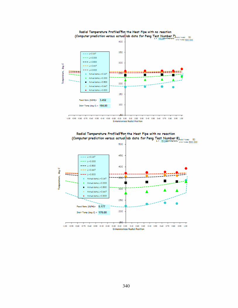
340
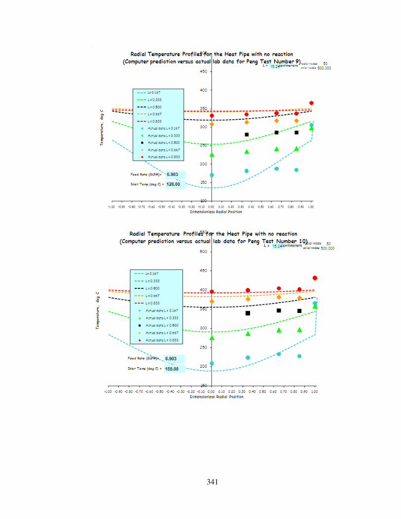
341

342

343
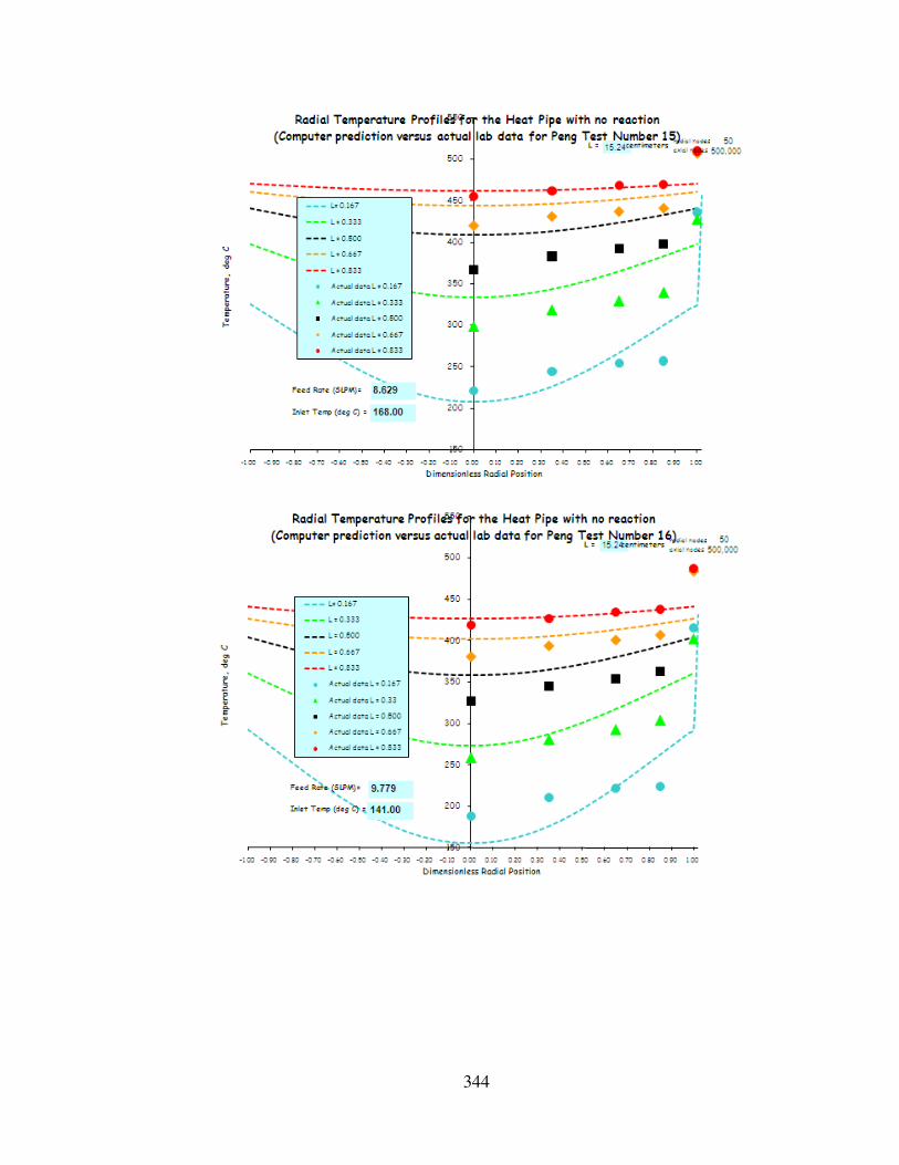
344
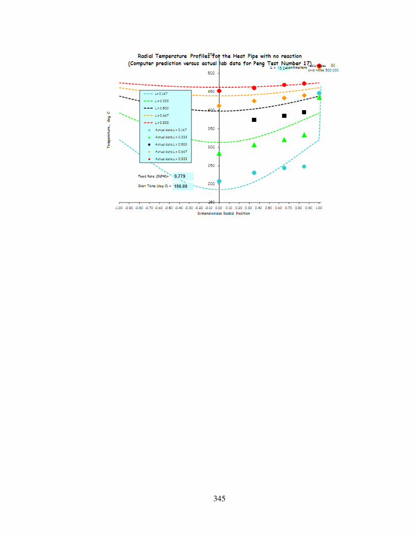
345

346
Appendix 4
Appendix 4 (Continued)
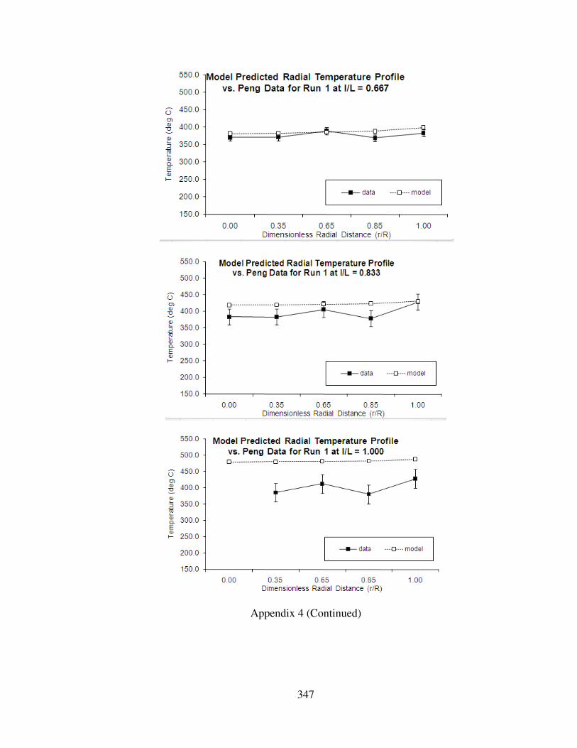
347
Appendix 4 (Continued)

348

349
Appendix 4 (Continued)
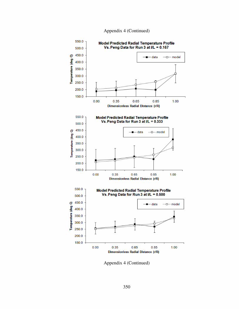
350
Appendix 4 (Continued)
Appendix 4 (Continued)
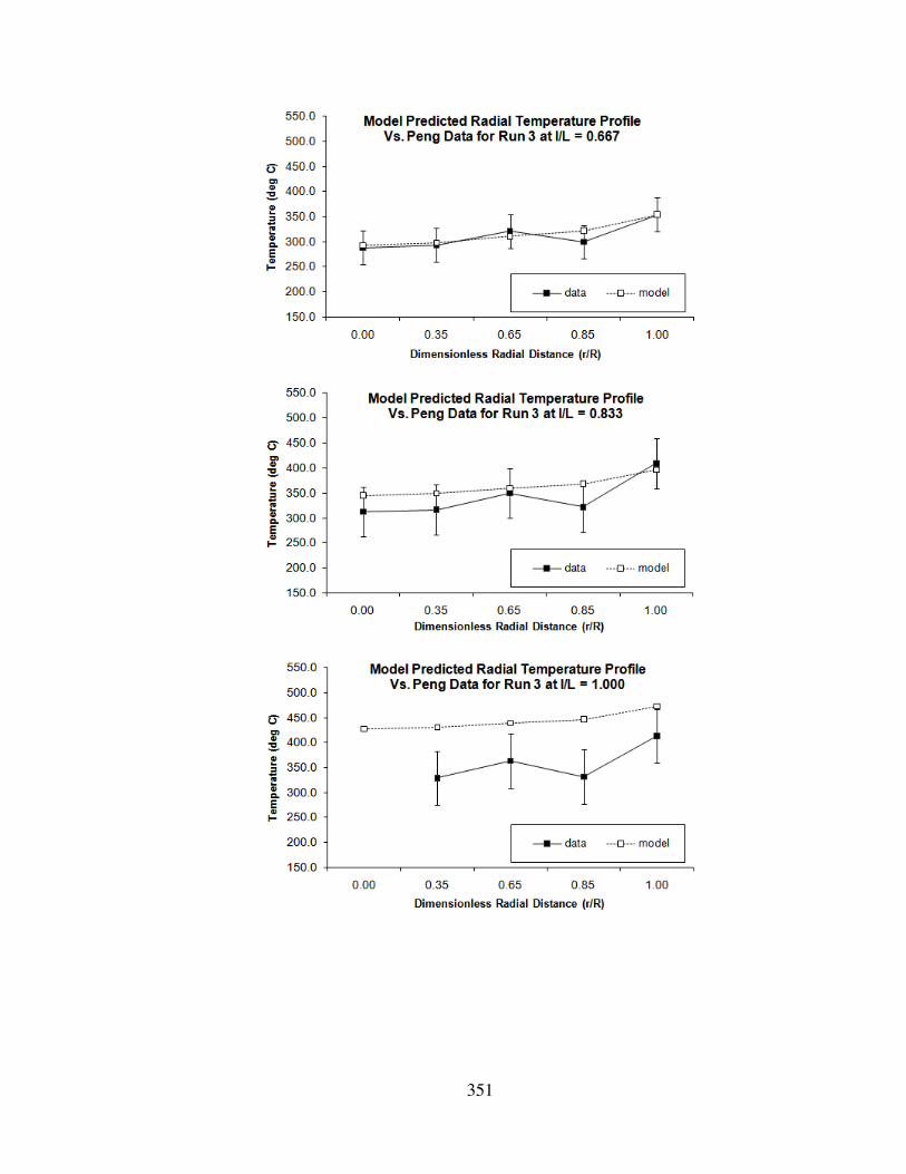
351

352
Appendix 4 (Continued)
Appendix 4 (Continued)

353
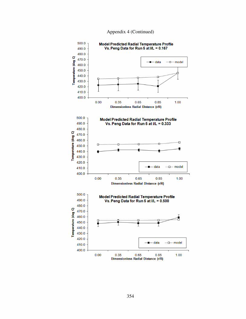
354
Appendix 4 (Continued)

355
Appendix 4 (Continued)
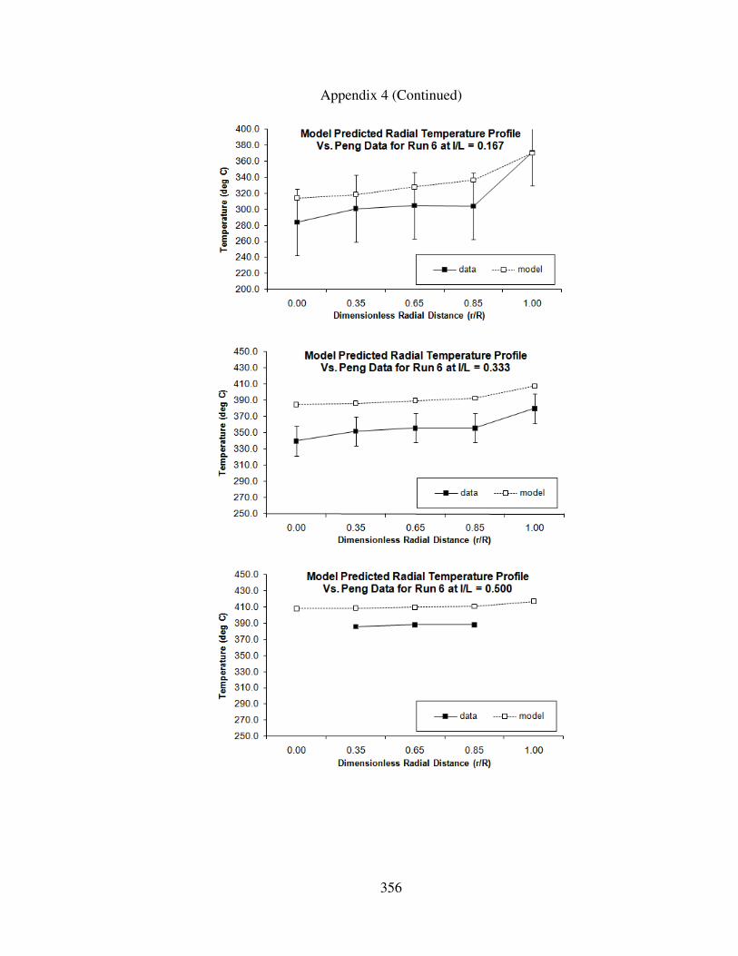
356
Appendix 4 (Continued)

357
Appendix 4 (Continued)

358
Appendix 4 (Continued)
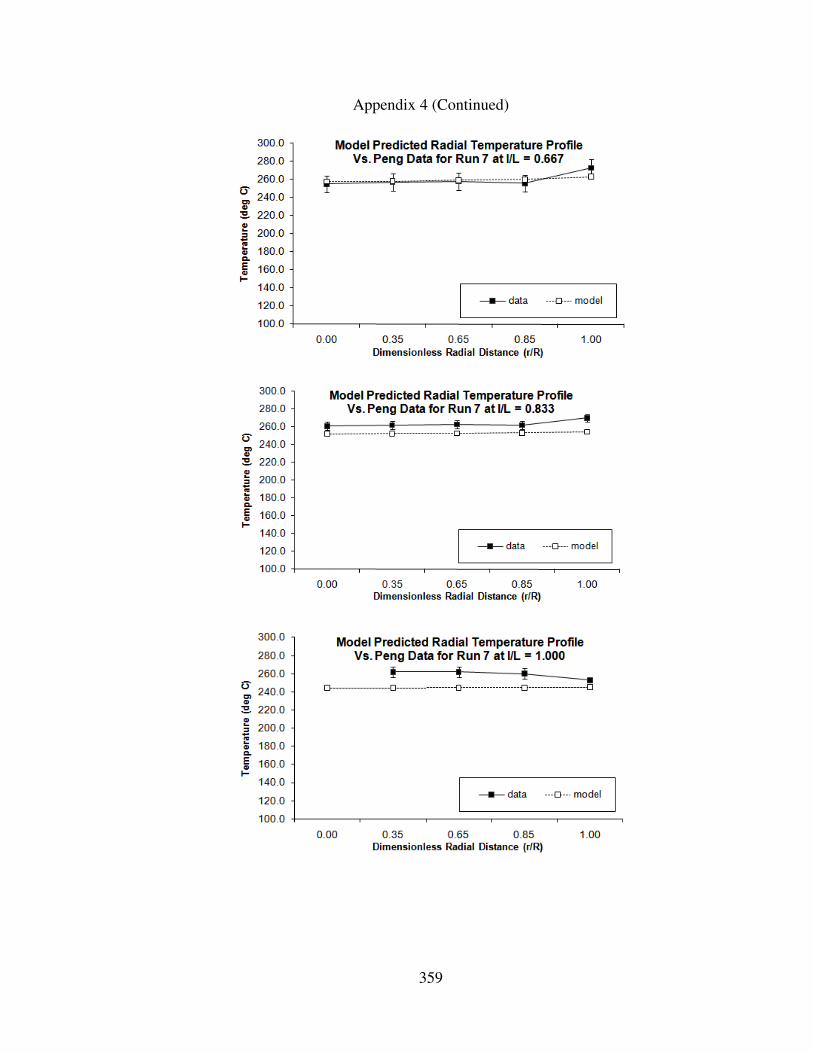
359
Appendix 4 (Continued)
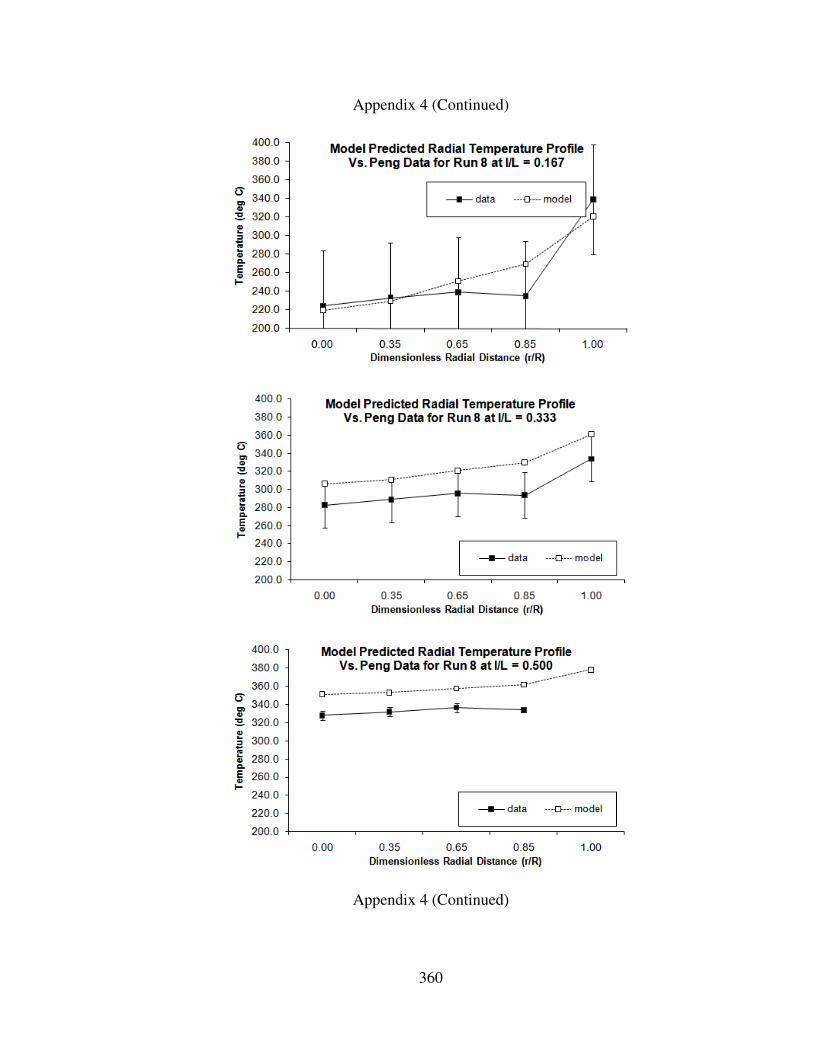
360
Appendix 4 (Continued)
Appendix 4 (Continued)

361

362
Appendix 4 (Continued)
Appendix 4 (Continued)
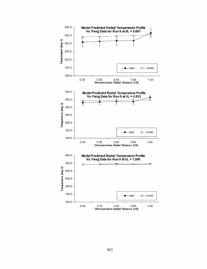
363

364
Appendix 4 (Continued)
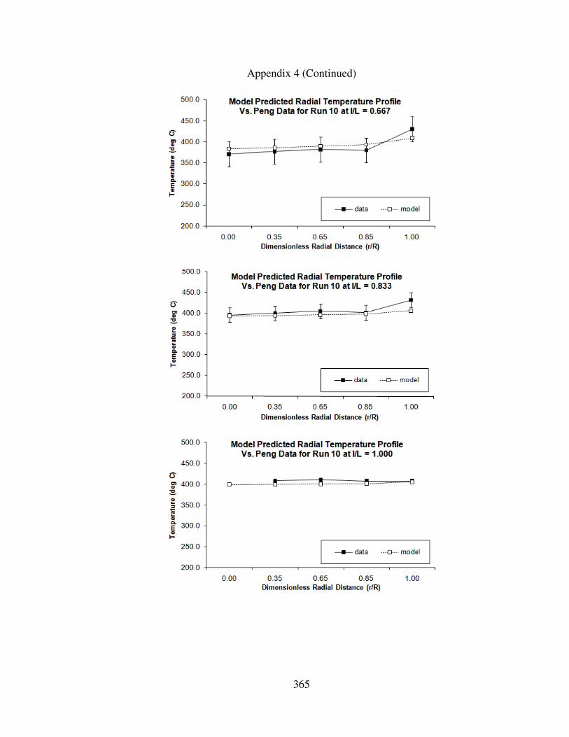
365
Appendix 4 (Continued)

366
Appendix 4 (Continued)

367
Appendix 4 (Continued)

368
Appendix 4 (Continued)
Appendix 4 (Continued)

369
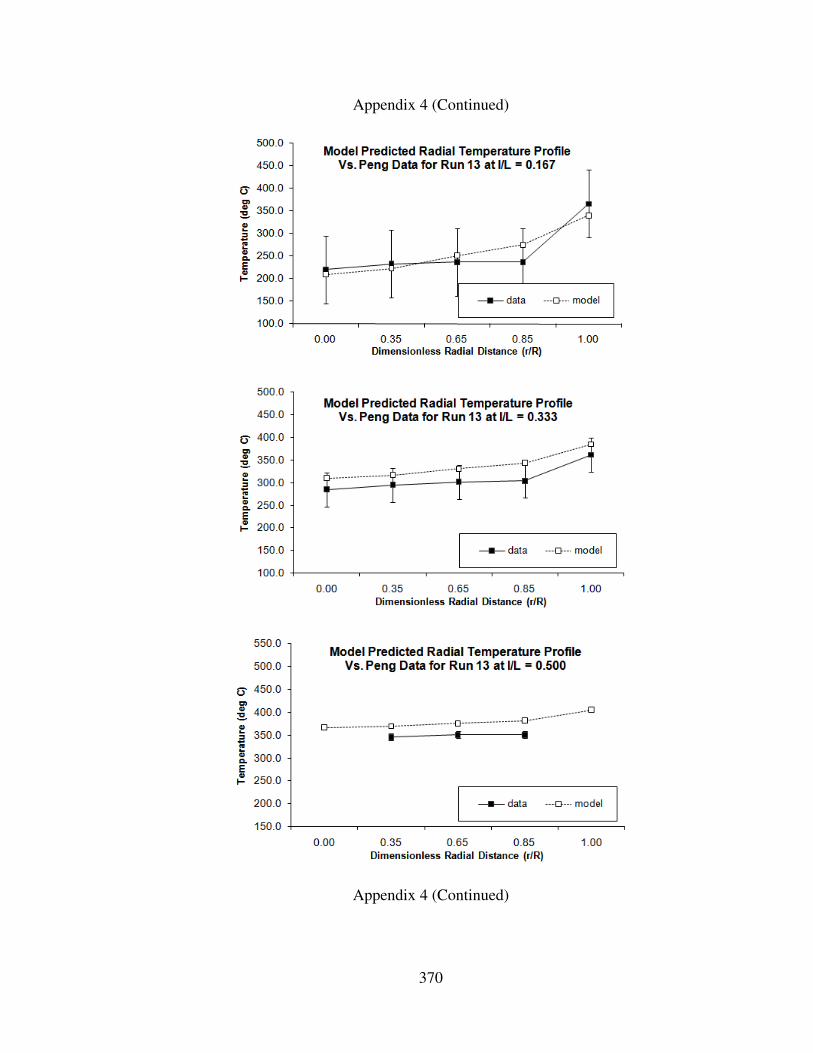
370
Appendix 4 (Continued)
Appendix 4 (Continued)

371
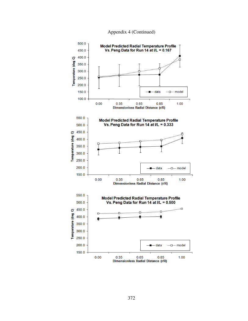
372
Appendix 4 (Continued)
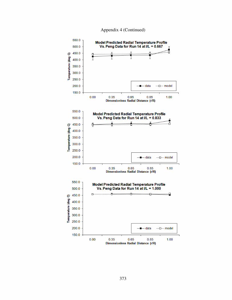
373
Appendix 4 (Continued)

374
Appendix 4 (Continued)
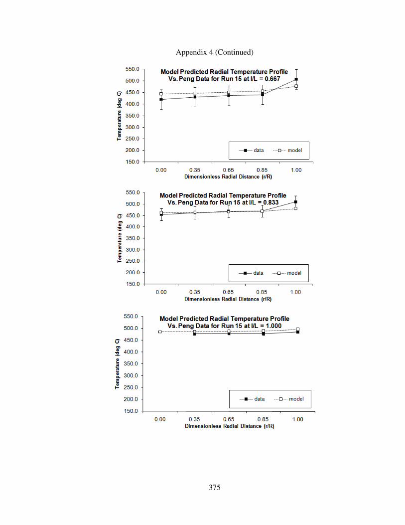
375
Appendix 4 (Continued)

376
Appendix 4 (Continued)

377
Appendix 4 (Continued)
Appendix 4 (Continued)
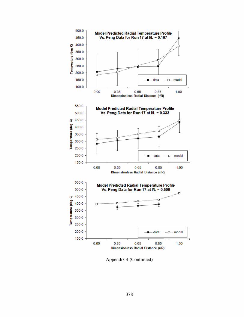
378
Appendix 4 (Continued)
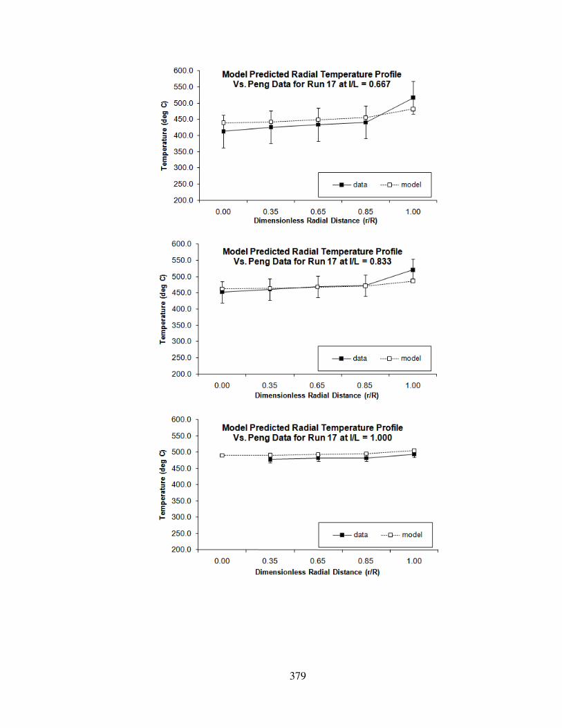
379

380
Appendix 5
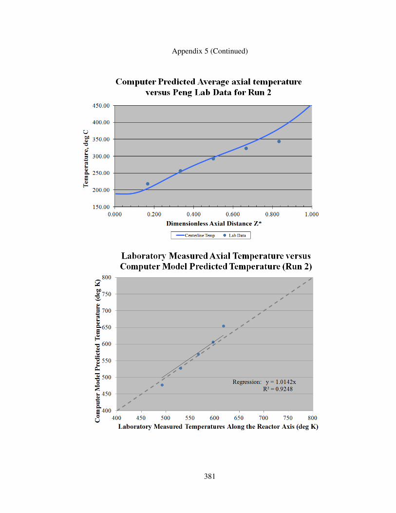
381
Appendix 5 (Continued)
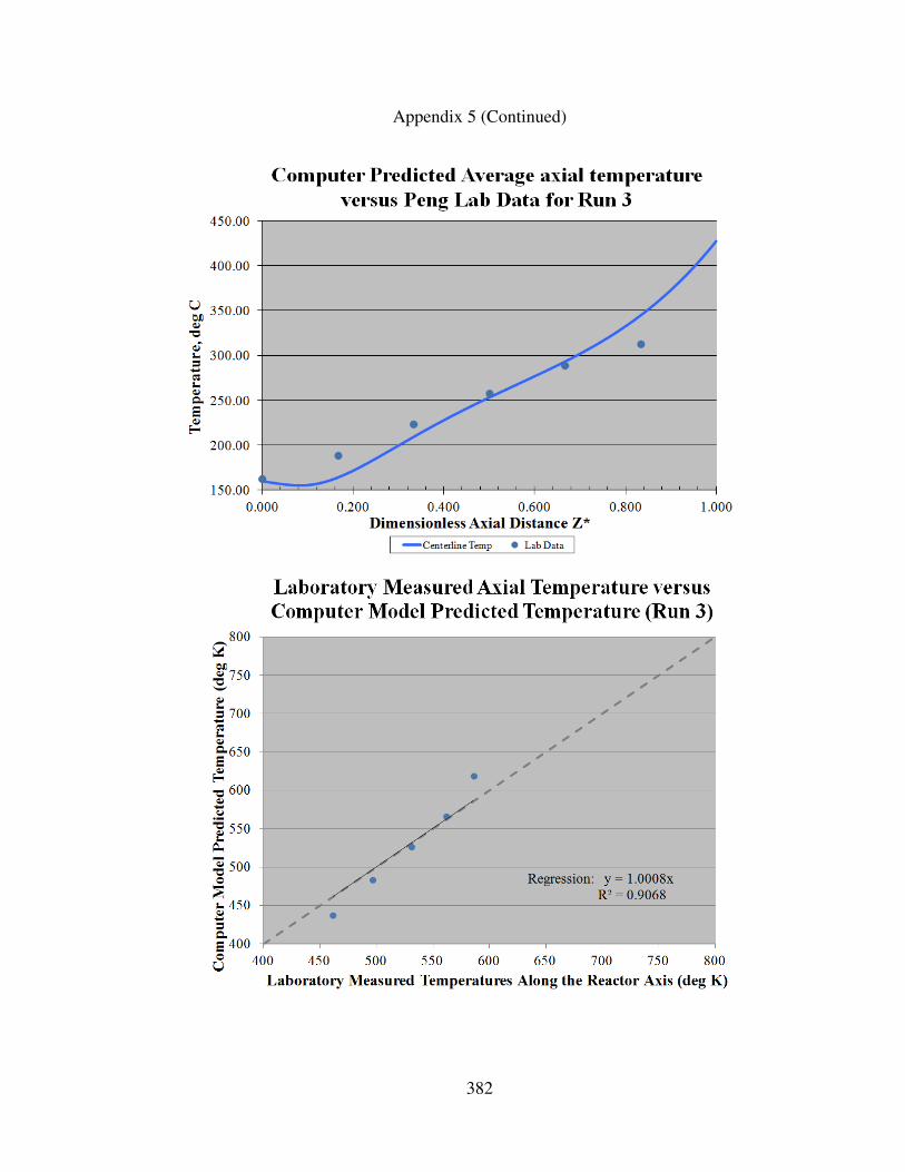
382
Appendix 5 (Continued)
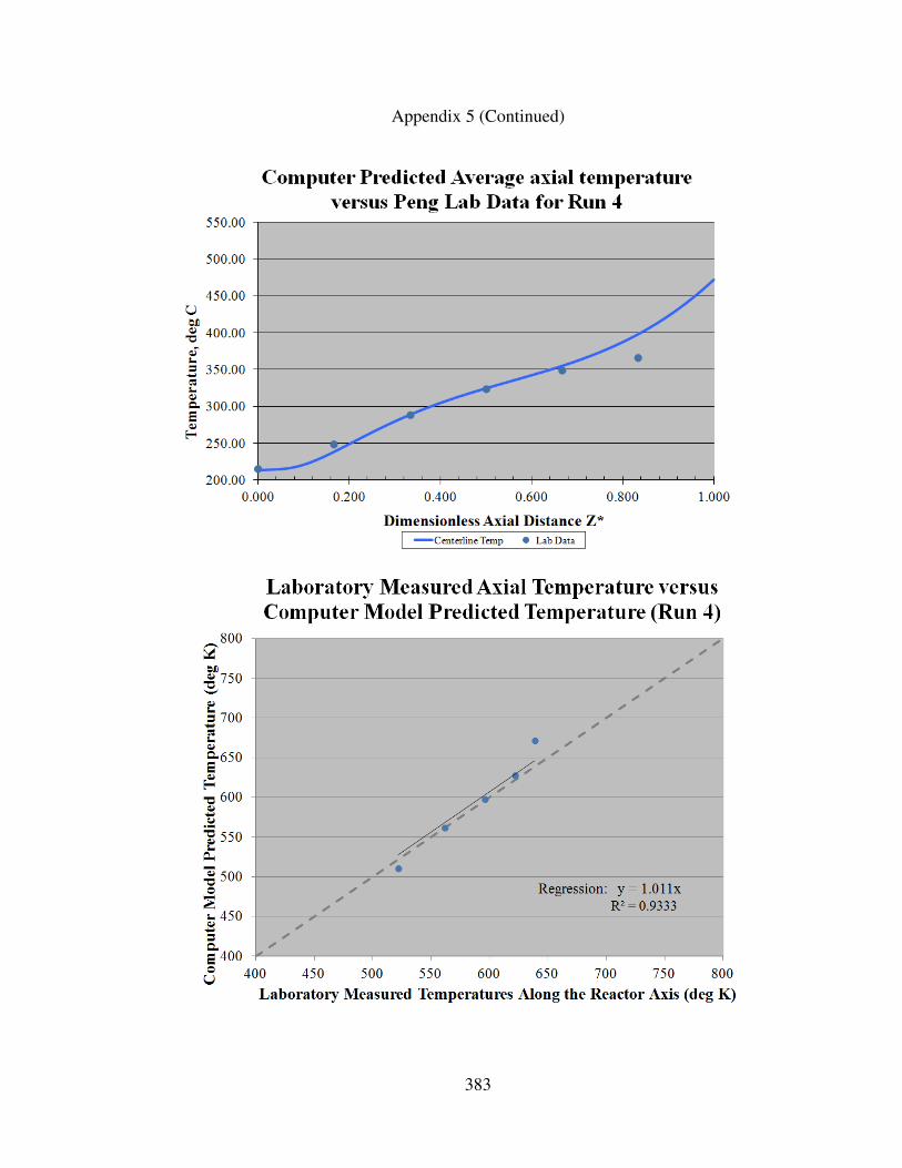
383
Appendix 5 (Continued)
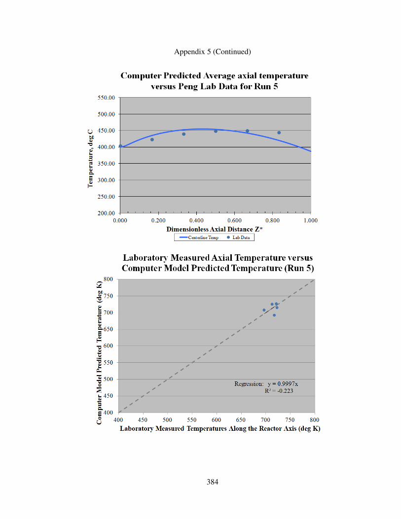
384
Appendix 5 (Continued)

385
Appendix 5 (Continued)
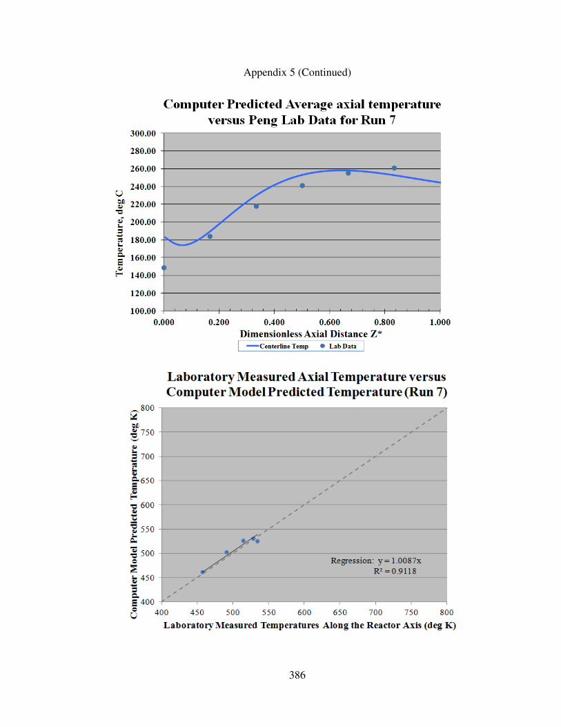
386
Appendix 5 (Continued)

387
Appendix 5 (Continued)

388
Appendix 5 (Continued)

389
Appendix 5 (Continued)

390
Appendix 5 (Continued)

391
Appendix 5 (Continued)
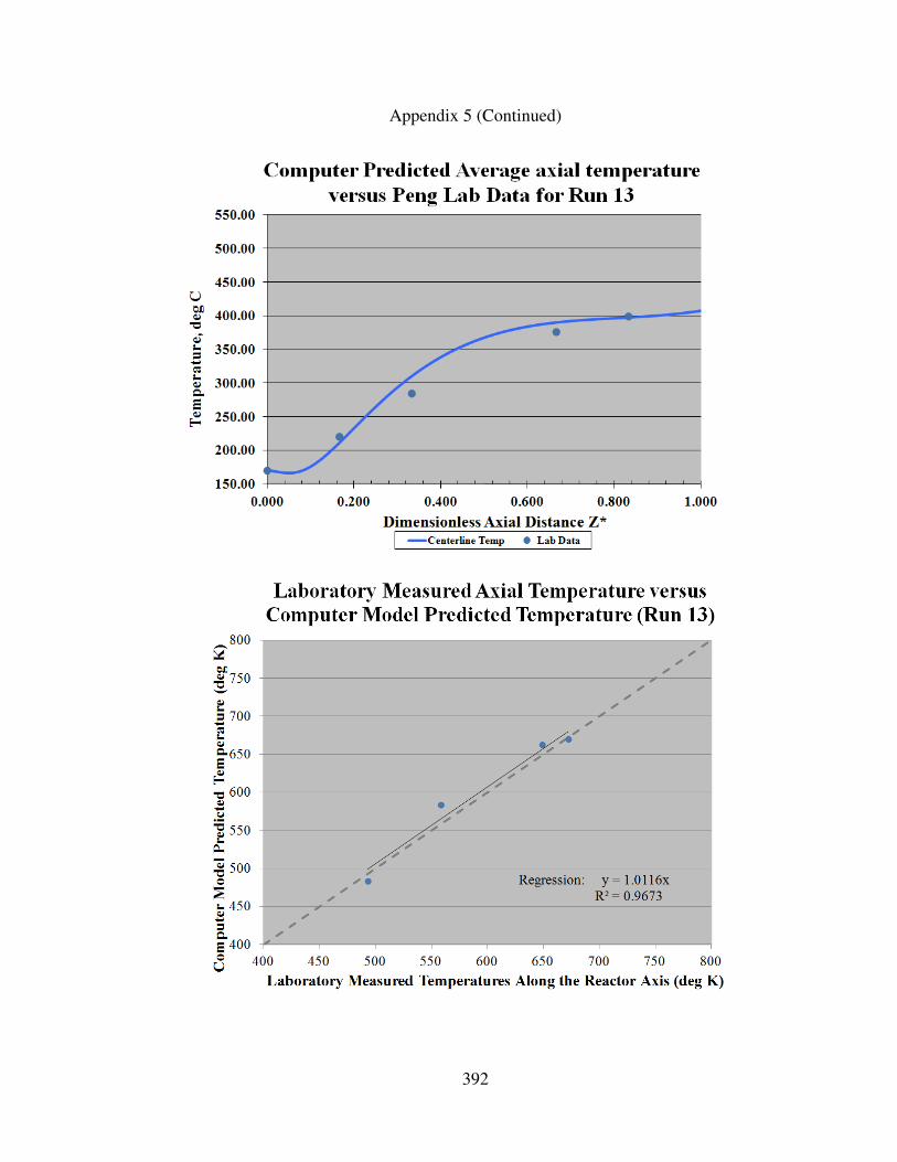
392
Appendix 5 (Continued)

393
Appendix 5 (Continued)

394
Appendix 5 (Continued)

395
Appendix 5 (Continued)

396
Appendix 5 (Continued)

397
Appendix 6 – H2A Input sheets
Technical operating parameters
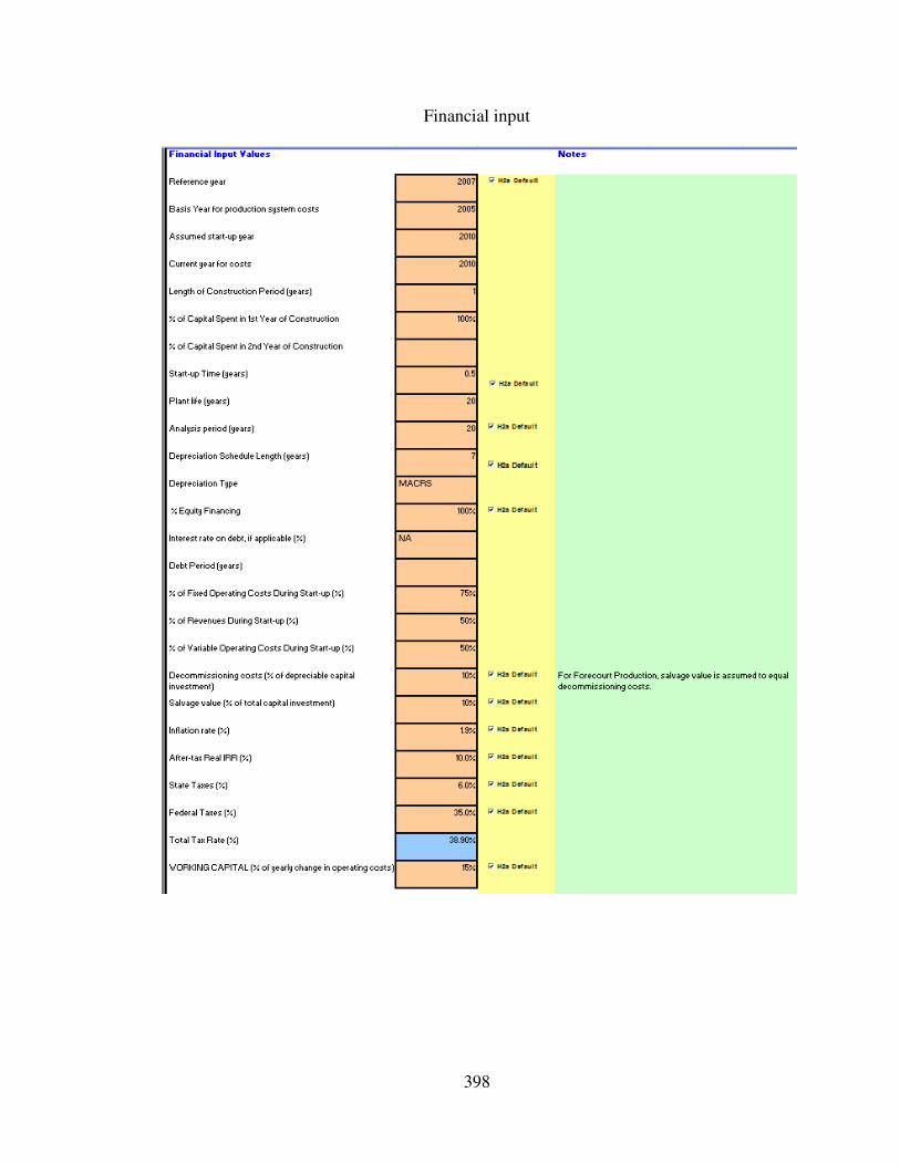
398
Financial input

399
Capital costs – hydrogen production

400
Fixed operating costs
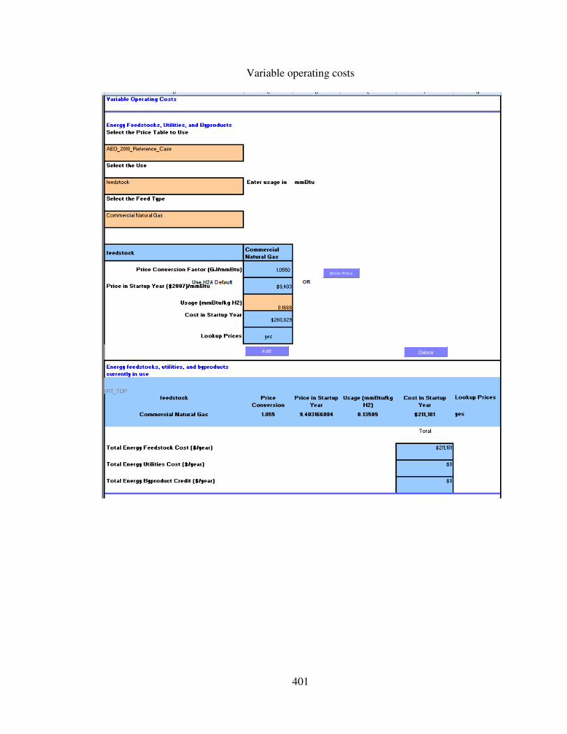
401
Variable operating costs
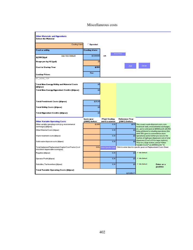
402
Miscellaneous costs

403
Capital costs

404
Refueling station costs

405