Copyright by Shawn Catherine McCleskey 2003

Copyright

by

Shawn Catherine McCleskey

2003

The Dissertation Committee for Shawn Catherine McCleskey Certifies that

this is the approved version of the following dissertation:

OPTICAL SIGNALING STRATEGIES FOR USE IN A MULTI-

COMPONENT SENSOR ARRAY

Committee:

Eric V. Anslyn, Supervisor

John T. McDevitt, Co-Supervisor

Dean Neikirk

Jason Shear

David Vanden Bout



by

SHAWN CATHERINE MCCLESKEY, B.S.

DISSERTATION

Presented to the Faculty of the Graduate School of

The University of Texas at Austin

in Partial Fulfillment

of the Requirements

for the Degree of

DOCTOR OF PHILOSOPHY

The University of Texas at Austin

August, 2003

Dedication

To family and friends who have faithfully walked alongside me. This journey

bears the indelible marks of your love.

v

Acknowledgements

There are many people to whom I would like to thank for their help and

encouragement during my graduate career at the University of Texas at Austin.

First, my advisors, Drs. Eric V. Anslyn and John T. McDevitt, were fundamental

to my success. Their guidance and tutelage allowed me to mature and grow as a

researcher. Thank you for supporting me and believing in my research abilities

even when I may have had my own doubts. Without your help, this work would

not have been possible.

I am grateful for the suggestions and contributions of the members of my

dissertation committee: Dr. Dean Neikirk, Dr. Jason Shear, and Dr. Vanden Bout.

I appreciate the time that you each generously spent with me throughout my

studies.

I also wish to extend my gratitude to each of the Anslyn and McDevitt

research group members. I am particularly indebted to Dr. Scott Bur, Dr. Mary

Jane Gordon, Dr. John J. Lavigne, and Dr. Stephen Schneider. Not only did you

help me through the program, you helped me gain a perspective outside of

chemistry. Additionally, I would like to acknowledge my good friends and

colleagues, Mike Griffin, Brenda Holtzman (Postnikova), and Angie Loving

vi

(Steelman) for your insightful advice and friendship. All of you made Welch Hall

a more pleasant environment in which to work.

Finally, I wish to thank my family and friends for being so patient with me

these past few years. Mom, Foster, Grandma H., Aunt Karen, and Collin, I thank

you for your inspiration and for always being proud of me. I want to thank my

close friends Jennifer Fogell, Emma Forsyth, Lee Melhorn (Fisher), and Pei-Ling

Wang for extending their friendship to me and keeping me well balanced. To my

best friend, Rachael Cobler, I am grateful to you for always believing in me and

for lending me a compassionate ear over and over again. And then there is my

dear Marco Rimassa. I love you and I will always keep your encouraging words

in my heart. Last, I wish to thank my Lord for whom I owe everything and I

praise Him through this work.

vii



Publication No._____________

Shawn Catherine McCleskey, Ph.D.

The University of Texas at Austin, 2003

Supervisor(s): Eric V. Anslyn and John T. McDevitt

This dissertation consists of four chapters that focus on various methods

and signaling strategies by which different analytes in solution can be detected

within a multi-component sensor array. The first chapter of this dissertation is a

review of recent work in the area of chemical sensing. A discussion is provided

here of the concepts and basic mechanisms required for a sensing event and

different approaches to designing molecular receptors. Next, chemical sensing is

described through examples of detection strategies documented in the literature.

The introductory chapter concludes by relating different sensory mimics to

current methods for vapor and solution phase analyte detection using

multicomponent sensor arrays and discussing the importance of pattern

recognition protocols for the successful application of sensor arrays.

viii

Chapter 2 discusses competitive indicator-displacement methods for the

solution-based UV-Visible analysis of citrate and calcium in beverages. A host

compound containing three guanidinium moieties on a triethylbenzene core is

employed to bind citrate. Improvements to the sensing scheme via

complexometric dyes known to bind calcium ion and the host are described.

Application of artificial neural networks to the spectral data also allowed for the

evaluation of citrate and calcium concentrations in flavored vodkas.

Chapter 3 describes a new sensing protocol by coupling a combinatorial

library of resin-bound receptors to a multi-component sensor array. The anchored

receptor includes a rationally designed scaffold with peptide libraries and is used

to bind various nucleotide phosphates. Analyte detection is accomplished by a

competition assay using fluorescein as the signaling compound. Principal

component analysis shows that the sensing ensembles create a fingerprint

response for each compound analyzed in the sensor array.

Chapter 4 applies the combinatorial array sensor system described in the

previous chapter toward the detection of nerve agent hydrolysis products. First,

the synthesis of a control resin-bound peptide library is presented to elucidate the

role of the scaffold plays in binding analytes. Studies that lend to an

understanding of the sensing protocol mechanism are discussed next in the

context of redesigning and optimizing assay conditions. The importance of data

processing on the outcome of the principal component analysis is also described.

Finally, ideas for expanding the utility of this sensing protocol toward the

detection of other classes of analytes via the combinatorial approach are proposed.

ix

Table of Contents

List of Tables........................................................................................................xiii

List of Figures ....................................................................................................... xv

List of Schemes ..................................................................................................xxiii

CHAPTER 1: INTRODUCTION 1

1.0 Scope .............................................................................................................. 1

1.1 Chemical Sensing........................................................................................... 2 1.1.1 Molecular Recognition Basics .............................................................. 3 1.1.2 Approaches to Molecular Receptors ..................................................... 7

1.2 Signaling Strategies...................................................................................... 11 1.2.1 Competition Assays............................................................................. 13 1.2.2 Microenvironmental Change............................................................... 14 1.2.3 Energy Transfer.................................................................................. 17

1.3 Multi-Analyte Sensing ................................................................................. 19 1.3.1 Sensory Mimics................................................................................... 21 1.3.2 Pattern Recognition ............................................................................. 26

x

1.4 Outlook......................................................................................................... 35

CHAPTER 2: COMPETITIVE INDICATOR METHODS USED FOR THE ANALYSIS OF CITRATE AND CALCIUM IN BEVERAGES 38

2.0 Introduction .................................................................................................. 38

2.1 Development of a Host for Citrate ............................................................... 39

2.2 Binding Studies ............................................................................................ 43 2.2.1 Selection of the Indicators and Experimental Conditions................... 43 2.2.2 Binding Stoichiometry ........................................................................ 44 2.2.3 Binding Data ....................................................................................... 45 2.2.4 Derivation of Binding Equations......................................................... 47 2.2.5 Curve Fitting Analysis ........................................................................ 51

2.3 Beverage Analysis........................................................................................ 56 2.3.1 Citrate in Beverages ............................................................................ 56 2.3.2 Citrate and Calcium in Beverages Using Artificial Neural

Networks ............................................................................................. 58

2.4 Summary ...................................................................................................... 65

2.5 Experimental .................................................................................................. 67 2.5.1 Materials.............................................................................................. 67 2.5.2 Absorption Studies .............................................................................. 67 2.4.3 Extraction of Binding Constants ......................................................... 68 2.5.4 Evaluation of Beverages...................................................................... 69 2.5.6 Neural Network Processing................................................................. 70

xi

CHAPTER 3: DIFFERENTIAL RECEPTORS CREATE PATTERNS DIAGNOSTIC FOR NUCLEOTIDE PHOSPHATES 71

3.0 Introduction .................................................................................................. 71

3.1 Development of Combinatorial Receptors for Nucleotide Phosphates........ 72

3.2 Array Platform Studies................................................................................. 76 3.2.1 Selection of Indicator and Experimental Conditions .......................... 76 3.2.2 Assay Optimization ............................................................................. 77

3.3 Nucleotide Phosphate Detection .................................................................. 87 3.3.1 Binding Data ....................................................................................... 87 3.3.2 Application of Principal Component Analysis.................................... 90 3.3.3 Sequencing results............................................................................... 91

3.4 Summary ...................................................................................................... 94

3.5 Experimental ................................................................................................ 95 3.5.1 Materials.............................................................................................. 95 3.5.2 Synthesis of control Chemosensors..................................................... 95 3.5.3 Instrumentation.................................................................................... 96 3.5.4 Assay Conditions................................................................................. 97 3.5.5 Data Collection and Processing........................................................... 97 3.5.6 Peptide Sequencing ............................................................................. 98

CHAPTER 4: DETECTION OF NERVE AGENT DEGRADATION PRODUCTS IN WATER BY A COMBINATORIAL ARRAY SENSOR SYSTEM 99

4.0 Introduction .................................................................................................. 99

4.1 Evaluating Chemosensor Microenvironments ........................................... 101 4.1.1 Design and Synthesis of “Control” Resin-Bound Library ................ 101 4.1.2 Array Platform Studies...................................................................... 104 4.1.3 Sequencing Results .......................................................................... 106

xii

4.2 Nerve Agent Degradation Product Detection............................................. 108 4.2.1 Assay Optimization ........................................................................... 108 4.2.2 Binding Data ..................................................................................... 109 4.2.3 Data Input Strategies for Principal Component Analysis ................ 112

4.3 Summary .................................................................................................... 115

4.4 Experimental ................................................................................................ 117 4.4.1 Materials............................................................................................ 117 4.4.2 Synthesis of “Control” Resin-Bound Library (4.1)........................... 118 4.4.3 Assay Conditions............................................................................... 119

Final Perspective ................................................................................................. 121

References ......................................................................................................... 122

Vita .................................................................................................................... 134

xiii

List of Tables

Table 1.1: Examples of electrostatic functional groups and their potential

counterions found in Nature and synthetic systems. .......................... 4

Table 1.2: Example data for PCA where m is the number of samples tested, s

represents a measurement response, and n is the number of

sensors used in the study. [The sample examples are adenosine

5’-triphosphate (ATP) and adenosine 5’-triphosphate (ATP).] ....... 27

Table 2.1: Concentration of citrate (mM) in beverages determined by

different sensing systems. The reported values shown are the

average value + standard deviation of three measurements. ............ 58

Table 2.2: (A) Concentration of citrate (mM) and calcium (mM) in the

validation test points samples determined by the two-component

sensing system and ANN analysis. The reported values shown

are the average value + standard deviation of three measurements

with the percent different shown in parenthesis. (B)

Concentration of citrate (mM) and calcium (mM) in various

flavored Smirnoff ® vodkas determined by ANN and NMR

analysis. ............................................................................................ 64

xiv

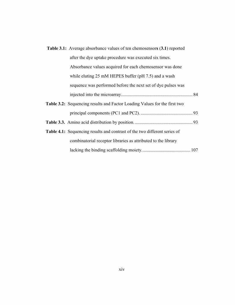
Table 3.1: Average absorbance values of ten chemosensors (3.1) reported

after the dye uptake procedure was executed six times.

Absorbance values acquired for each chemosensor was done

while eluting 25 mM HEPES buffer (pH 7.5) and a wash

sequence was performed before the next set of dye pulses was

injected into the microarray.............................................................. 84

Table 3.2: Sequencing results and Factor Loading Values for the first two

principal components (PC1 and PC2). ............................................. 93

Table 3.3. Amino acid distribution by position. .................................................. 93

Table 4.1: Sequencing results and contrast of the two different series of

combinatorial receptor libraries as attributed to the library

lacking the binding scaffolding moiety. ......................................... 107

xv

List of Figures

Figure 1.1: Benzene used as an example for π-interactions. (A) General

molecular structure of benzene. (B) Electrostatic potential of

benzene with areas of negative charge above and below the plane

with a positive charge in the plane of the molecule. .......................... 5

Figure 1.2: Temporary and induced dipoles in nonpolar molecules due to the

nonuniform distribution of electrons at any given moment. .............. 6

Figure 1.3: Optical signaling mechanism: Upon binding of the analyte, a

sensing element will have a detectable response.43.......................... 13

Figure 1.4: A competition assay allows for the presence on an analyte to be

detected upon displacement of an indicator molecule...................... 14

Figure 1.5: The ionization state of the pH sensitive probe

carboxyfluorescein.56........................................................................ 15

Figure 1.6: Schematic representation of the proposed sensor mechanism for

dansyl modified CDs upon addition of guests.43.............................. 16

Figure 1.7: Overlap integral (shaded area) for energy transfer from a donor

molecule (dashed line) to an acceptor molecule (solid line). ........... 17

Figure 1.8: Shift in approaches taken for chemical sensing. (A) “Lock and

Key” approach to host-guest systems. (B) Library of receptors

approach.43........................................................................................ 20

Figure 1.9: Schematic of micromachined chemosensor array (“electronic

tongue”).43 ........................................................................................ 22

xvi

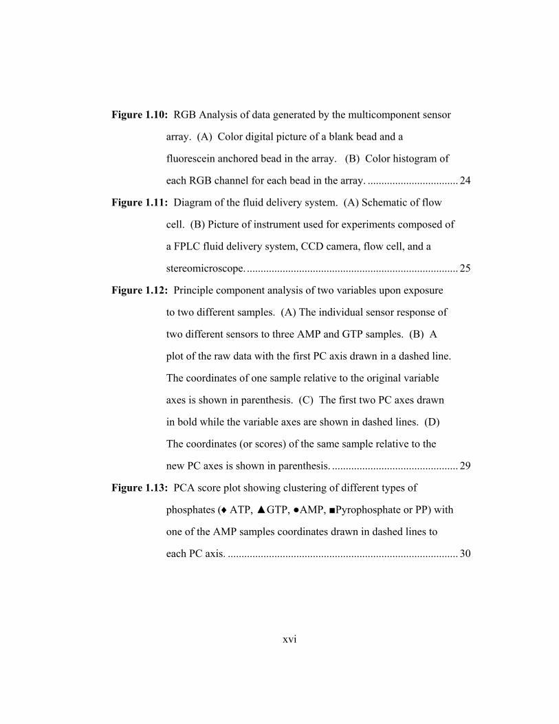
Figure 1.10: RGB Analysis of data generated by the multicomponent sensor

array. (A) Color digital picture of a blank bead and a

fluorescein anchored bead in the array. (B) Color histogram of

each RGB channel for each bead in the array. ................................. 24

Figure 1.11: Diagram of the fluid delivery system. (A) Schematic of flow

cell. (B) Picture of instrument used for experiments composed of

a FPLC fluid delivery system, CCD camera, flow cell, and a

stereomicroscope. ............................................................................. 25

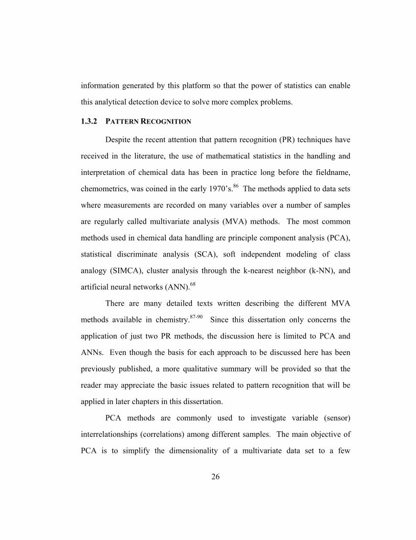
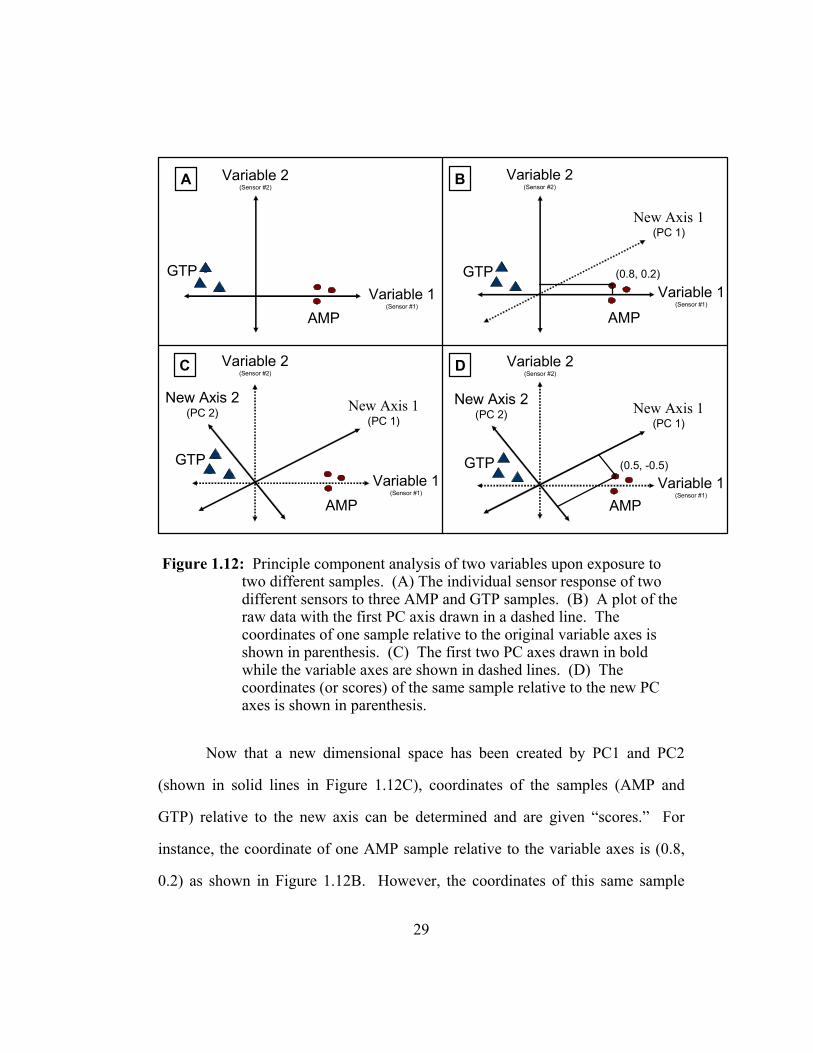
Figure 1.12: Principle component analysis of two variables upon exposure

to two different samples. (A) The individual sensor response of

two different sensors to three AMP and GTP samples. (B) A

plot of the raw data with the first PC axis drawn in a dashed line.

The coordinates of one sample relative to the original variable

axes is shown in parenthesis. (C) The first two PC axes drawn

in bold while the variable axes are shown in dashed lines. (D)

The coordinates (or scores) of the same sample relative to the

new PC axes is shown in parenthesis. .............................................. 29

Figure 1.13: PCA score plot showing clustering of different types of

phosphates (♦ATP, ▲GTP, ●AMP, ■Pyrophosphate or PP) with

one of the AMP samples coordinates drawn in dashed lines to

each PC axis. .................................................................................... 30

xvii

Figure 1.14: Operation of a single “neuron” or input unit in an FF-MLP

ANN. A summation of all input signals are subjected to a weight

(Wnj) and transfer function before sent on as an output (Outj) to

the next “neuron.” ............................................................................ 33

Figure 1.15: A diagram of a three layered FF-MLP ANN. The ANN is

composed of an input layer, a variable number of hidden layers,

and an output layer. .......................................................................... 34

Figure 2.1: UV-Vis spectra of 2.3 in 25% (v/v) water in methanol with 5 mM

HEPES buffer at pH 7.4. Addition of 2.1 to a solution of 2.3 at

constant concentration (14 µM) causes an increase in absorbance

at 495 nm (arrows indicate the direction of change in the

absorbance intensity).92 .................................................................... 41

Figure 2.2: UV-Vis spectra of 2.3 in 25% (v/v) water in methanol with 5 mM

HEPES buffer at pH 7.4. Addition of 2.2 to the sensing

ensemble 2.1:2.3 at constant concentration (75 µM 2.1, 14 µM

2.3) causes a decrease in absorbance at 495 nm (arrows indicate

the direction of change in the absorbance intensity).92 .................... 42

Figure 2.3: UV-Vis spectra of 2.4 in 25% (v/v) water in methanol with 10

mM HEPES buffer at pH 7.5. Addition of 2.1 to a solution of

2.4 at constant concentration (55 µM) causes and increase of

absorbance at 577 nm and a decrease in absorbance at 445 nm

(arrows indicate the direction of change in the absorbance

intensity)........................................................................................... 46

xviii

Figure 2.4: UV-Vis spectra of 2.5 in 25% (v/v) water in methanol with 10

mM HEPES buffer at pH 7.5. Addition of 2.1 to a solution of

2.5 at constant concentration (55 mM) causes an increase in

absorbance at 607 nm and a decrease in absorbance at 454 nm

(arrows indicate the direction of change in the absorbance

intensity)........................................................................................... 47

Figure 2.5: UV-Vis spectra of 2.4 and 2.5 in 25% (v/v) water in methanol

with 10 mM HEPES buffer at pH 7.5. (A) Addition of 2.2 to a

solution of 2.4:2.1 at constant concentration (55 µM 2.4, 1.13

mM 2.1) causes a decrease in absorbance at 577 nm and an

increase in absorbance at 445 nm. (B) Addition of 2.2 to a

solution of 2.5:2.1 at constant concentration (55 µM 2.5, 1.13

mM 2.1) causes a decrease in absorbance at 607 nm and an

increase of absorbance at 454 nm (arrows indicate the direction

of change in the absorbance intensity) ............................................. 52

Figure 2.6: Theoretical fit (-) of Eq. 2.17 to the experimental data (○)

obtained from ∆A as a function of the addition of 2.1 to each

indicator. (A) Isotherm plot for addition of 2.1 to 2.4 (λ =

577nm). (B) Isotherm plot for the addition of 2.1 to 2.5 (λ =

607nm). ............................................................................................ 54

xix

Figure 2.7: Calibration curves used for the citrate assay (25% (v/v) water in

methanol with 10 mM HEPES buffer at pH 7.5). (A) UV-Vis

calibration curve using 2.4 at the indicator (55 µM 2.4, 1.13 mM

2.1, λ = 577 nm). (B) UV-Vis calibration curve using 2.5 at the

indicator (55 µM 2.5, 1.13 mM 2.1, λ = 607 nm). ........................... 57

Figure 2.8: The approach taken to obtain data via UV-Vis spectroscopy for

the two-component sensing ensemble, where spectra were

recorded at various concentrations (mM) of calcium and citrate..... 60

Figure 2.9: Representative UV-Vis spectra of the indicator-displacement

assays created when a solution containing 2.4 (240 µM) and 2.1

(10 µM) is titrated with various concentrations of calcium and

2.2 in 25% (v/v) vodka in water with 10 mM HEPES buffer at

pH 7.5. [(▬)Calcium at 400 µM and citrate at 100 µM] and [(─

─) Calcium at 50 µM and citrate at 600 µM] Inside tick marks

on the x-axis illustrate the 25 wavelengths chosen to use in the

ANN analysis. .................................................................................. 61

Figure 2.10: General representation of the multilayer ANN used for the

analysis of flavored vodkas. The ANN is composed of an input

layer, a variable number of hidden layers, and an output layer........ 63

xx

Figure 3.1: Isotherm plots of the Ser-Tyr-Ser library (3.3) member in 200

mM HEPES buffer solution at pH 7.4. Comparison of

fluorescence response to additions of ATP, GTP, and AMP

solutions shows 3.3 selectivity of ATP over the other

phosphates.97 .................................................................................... 75

Figure 3.2: Signal transduction scheme used to detect nucleotide phosphates

within the resin-bound sensor (3.1). AAn = amino acid.................. 77

Figure 3.3: (A) Scanning electron micrograph of representative 3 x 4

microarray containing glass beads.114 (B) Design of flow cell

used in experiments. ......................................................................... 78

Figure 3.4: Differential dye (3.2) binding to the library of receptors (3.1,

Beads 3, 4, 6, 7, 10 and 12). (A) Representative image of the

chemosensors studied within the array after a solution of 3.2 was

introduced. (B) Graphical representation of the data taken by the

CCD camera upon an injection of 0.03 M solution of 3.2 to the

array of beads with eluting 25 mM HEPES buffer at pH 7.5.

(Bead #1 (3.4) took up little or no dye.)........................................... 80

Figure 3.5: Absorbance values plotted over time for an array containing four

members of 3.1 library in eluting 25 mM HEPES buffer at pH

7.5. (A) Addition (2.0 mL pulse) of 3.2 solution at 0.30 mM.

(B) Addition (2.0 mL pulse) of 3.2 solution at 3.0 mM................. 82

xxi

Figure 3.6: Absorbance values plotted over time elapsed (7 min) for 3.1:3.2

in eluting 25 mM HEPES buffer at pH 7.5 upon successive

cycles of dye uptake, 20 mM ATP solution injections, and the

wash sequence. ................................................................................. 86

Figure 3.7: Absorbance values plotted over time for 3.1:3.2 in eluting 25

mM HEPES buffer at pH 7.5. (A) Addition (2.0 mL pulse) of

20 mM GTP solution in 25 mM HEPES (pH 7.5). (B) Addition

(2.0 mL pulse) of 20 mM AMP solution in 25 mM HEPES (pH

7.5). To aid in slope comparison, the plots were shifted so that

the average of the initial 30 points prior to sample injection (not

shown) had an absorbance of 1.00. .................................................. 89

Figure 3.8: Principle component analysis plot of the three trials for each

nucleotide phosphate sample (▲ATP, ♦GTP, ■AMP). Red

circles have no statistical meaning and are only drawn to help aid

in sample comparison....................................................................... 91

Figure 3.9: Factor Loading Plot of the nine library (3.1) beads chosen for

microsequencing............................................................................... 92

Figure 4.1: (A) Schematic summarizing the split and pool method used to

generate each library of resin-bound receptors. (B) General

molecular structure of receptor library series 3.1. (C) General

molecular structure of “control” resin-bound peptide library 4.1. . 102

Figure 4.2: General synthetic scheme for solid phase synthesis of trimers on

TentaGel-NH2 resins. ..................................................................... 103

xxii

Figure 4.3: Dye uptake characteristics of the two different series of

combinatorial receptor libraries subjected to identical

experimental conditions. (A) Capacity of five random beads

selected from library series 4.1 to uptake dye from a 0.30 mM

solution of 3.2. (B) Capacity of five random beads selected

from library series 3.1 to uptake dye from a 0.30 mM solution of

3.2. .................................................................................................. 106

Figure 4.4: Absorbance values plotted over time for the 3.2:3.1 sensing

ensemble in eluting 25 mM HEPES buffer at pH 7.5 upon

addition (2.0 mL pulse) of two successive [(A) Trial #1 and (B)

Trial #2] 20 mM PMPA solutions in 25 mM HEPES (pH 7.5).

(●Bead 3, ○Bead 4,▲Bead 20, ■Bead 22, □Bead 26)................... 110

Figure 4.5: Graphical representation of multicomponent fingerprint

responses yielded by the sensing ensemble ( library series 1: dye

molecule) upon the introduction of (A) 20 mM MPA, (B) 20 mM

EMPA, and (C) 20 mM PMPA solution in 25 mM HEPES at pH

7.5. (■Bead 3, ■Bead 4, ■Bead 20, ■Bead 26)............................. 112

Figure 4.6: Principle component analysis plot of three trials for each CWA

degradation sample (▲MPA, ■EMPA, ●PMPA) with the raw

data inputted into Statistica (input strategy #1).............................. 114

Figure 4.7: Principle component analysis plot of three trials for each CWA

degradation sample (▲MPA, ■EMPA, ●PMPA) with data input

strategy #2. ..................................................................................... 115

xxiii

List of Schemes

Scheme 1.1: Molecular receptors containing a rationally designed scaffold.

General molecular structure of an anion recognition receptor

(1.1) using a xanthenene spacer produced by Umezawa.15

General molecular structure of a modified calyx[4]arene (1.2)

used to complex neutral guests created by Reinhoudt.16.............. 8

Scheme 1.2: Molecular receptors derived from the combinatorial approach.

The molecular structure of the receptor consisting of a

peptidosteroidal backbone and tripeptide arms (1.3) made by

Still.28 The molecular structure of the “tweezer receptor”

using a guanadinium binding site and two tripeptide arms

(1.4) created by Kilburn and Bradley.30 ..................................... 11

Scheme 1.3: Molecular structure of molecular thermometer created by

Fabbrizzi utilizing PET as the sensing strategy.64...................... 19

Scheme 2.1: Molecular structures of host (2.1) and 5-carboxyfluorescein

(2.3) ............................................................................................ 40

Scheme 2.2: Equilibria for the systems studied by UV-Vis spectroscopy. ......... 44

Scheme 2.3: Molecular structures of the host (2.1) and indicators (2.4 and

2.5) used to sense for citrate....................................................... 53

Scheme 2.4: Equilibria of the extended systems studied..................................... 62

Scheme 3.1: General molecular structure of combinatorial resin-bound

receptor library (3.1) and fluorescein (3.2) used to sense for

nucleotide phosphates in the array platform. ............................. 72

xxiv

Scheme 3.2: General molecular structure of initial combinatorial resin-bound

receptor library with attached fluorphores (3.3) used for

screening and conventional fluorometer studies of nucleotide

phosphates. ................................................................................. 73

Scheme 3.3: Molecular structures of the various nucleotide phosphates

studied. ....................................................................................... 88

Scheme 4.1: Common hydrolysis pathways for some nerve agents in water.... 100

1

CHAPTER 1: INTRODUCTION

1.0 Scope

The various methods and signaling strategies by which multiple analytes

in solution can be detected within a multicomponent sensor array define the scope

of this dissertation. The aim of this introductory chapter is to summarize

developments in the field of chemical sensing and their applications for analyte

detection. It reviews the relevant literature through June 2003. The first section

describes the basic properties and forces of molecular interactions associated with

host-guest chemistry. Also, concepts concerning preorganization, geometric

agreement and combinatorial libraries are presented in the context of different

approaches available to chemists for designing molecular receptors. The main

portion of this chapter is devoted to the development of sensors exploiting the

ideas described in Section 1.1 for applications in chemical sensing. This includes

several examples of signaling strategies documented in the literature for the

detection of various analytes. Several array-based approaches to multi-analyte

sensing are discussed next along with the different mathematical techniques used

to extract patterns from the large amounts of information generated by these

multicomponent sensor arrays. The chapter concludes by detailing how the

concepts presented in this chapter pertain to the chemical sensing applications

demonstrated throughout this dissertation.

2

1.1 Chemical Sensing

In order to sense the world around us, we rely upon what Nature has

provided us so that we can see, hear, touch, smell, and taste experiences present in

everyday life. In scientific terms, sensing allows us to evaluate our environment

by artificial means through methods and novel materials that mimic gustation,

olfaction, vision, and auditory stimulation usable in analyzing complex mixtures.

Of the five mammalian senses, gustation and olifaction are known as the

chemically derived senses and they provide the foundation from which our

response to chemical stimuli emulates. In this respect, many new sensor systems

broadly responsive to a large number of analytes have been developed recently

modeled in part by the sense of smell (vapor phase) and taste (solution phase).

Several examples of these sensory mimic systems are presented in more detail in

Section 1.3.3.

The nature of this subject is interdisciplinary, yet the roots of mimic

sensing are in chemistry, namely, molecular recognition. Chemical sensing is

accomplished by coupling a recognition element to a transduction element in

order to signal the presence of the analyte. Since the basis of chemical sensing

relies on a sensing element recognizing an analyte, the following section is

dedicated to a discussion about molecular recognition and the nature of host/guest

interactions. Examples of different methods used to develop molecular receptors

for application in chemical sensing are also presented.

3

1.1.1 MOLECULAR RECOGNITION BASICS

Molecular recognition refers to a host or receptor molecule that is capable

of associating with a particular guest molecule more strongly than with other

molecules. The reason for the tight association between the host and guest

molecule can be attributed to the presence of more favorable non-covalent

interactions between the two molecules. Non-covalent interactions typically seen

with the association between two molecules includes electrostatics, Van der

Waals forces, and hydrophobic interactions. Therefore, understanding molecular

recognition requires studying these types of interactions and how these

interactions in concert with each other help achieve host-guest complexes.

The most prevalent of the non-covalent interactions are the electrostatic

forces between two charged entities. In Nature, there are many examples that

scientists have learned from such as DNA base pairing, antibody-antigen

interactions, and substrate-enzyme complexes. These types of interactions

include charge pairing, hydrogen bonding, and ionic interactions. Some common

pairs of charged functional groups found in Nature and synthetic systems are

listed in Table 1.1.

4

Table 1.1: Examples of electrostatic functional groups and their potential counterions found in Nature and synthetic systems.

An important aspect of these types of interactions is their dependence on

pH and their solvation sphere. Since the enthalpic energies associated with

electrostatic interactions are calculated through Coulomb’s law (Eq 1.1), the

energy decreases inversely with the distance between the two entities.1 This

means that the interaction is stronger in a hydrophobic environment which forces

the two molecules in closer proximity and is weaker in an environment that

completely solvates the ionizable functionality. For instance, Nature will often

place the charged binding site of an enzyme in a hydrophobic pocket in order to

minimize its exposure to water and increase the electrostatic effect. However, the

opposite is observed when sodium chloride is placed in a polar protic solvent like

water. The two ions completely dissociate in water destroying the presence of an

electrostatic bonds.

carboxylate

phosphate

sulfate

phenoxide

Anions Cation Partners

ammoniums

guanidinium

metals

Structure

O

O

O

P OO

O

O

SO

O

O

O

Structure

H2N

NH

NH3

NH

NH2

NH

Ca(II), Zn(II),Mg(II), etc

carboxylate

phosphate

sulfate

phenoxide

Anions

carboxylate

phosphate

sulfate

phenoxide

Anions Cation Partners

ammoniums

guanidinium

metals

Cation Partners

ammoniums

guanidinium

metals

Structure

O

O

O

P OO

O

O

SO

O

O

O

Structure

O

O

O

P OO

O

O

SO

O

O

O

Structure

H2N

NH

NH3

NH

NH2

NH


Structure

H2N

NH

NH3

NH

NH2

NH


5

rZerE

)4()(

0

2

πε−

= Eq. 1.1

Other electrostatic interactions concerning aromatic compounds include π-

π and cation- π stacking.2 Sometimes referred to as a type of ionic interaction,

the basic concept of aromatic compounds aggregating to each other or

coordinating to cations can be explained by considering the electrostatic potential

associated with benzene (Figure 1.1). Here, areas of negative charge are seen

above and below the plane of the benzene molecule with a ring of positive

potential in the plane. Simple cations have been observed interacting strongly

with the negatively polarized face of benzene.3 Similarly, the attraction of the

negative face on one aromatic ring to the positive edge of another aromatic ring

has contributed to stabilizing DNA structures and the behavior observed with

some liquid crystals.4

Figure 1.1: Benzene used as an example for π-interactions. (A) General molecular structure of benzene. (B) Electrostatic potential of benzene with areas of negative charge above and below the plane with a positive charge in the plane of the molecule.

Van der Waals interactions (or London dispersion forces) are much

weaker forces than electrostatic interactions and account for a much smaller

portion in the energy of binding (1%).1 However, they are important when

A B

6

considering the interactions of molecules that do not contain charged groups.

Consider a nonpolar molecule like methane. Despite the fact that methane does

not have a permanent dipole moment, electrons are dynamic and are capable of

generating an instantaneous dipole that temporarily induces an opposite dipole in

a neighboring molecule (Figure 1.2). Even though these temporarily induced

dipoles are small, they do produce attractive forces between nonpolar molecules.

Figure 1.2: Temporary and induced dipoles in nonpolar molecules due to the nonuniform distribution of electrons at any given moment.

Another important non-covalent interaction to consider is the hydrophobic

effect that refers to the low solubility of hydrocarbons in water. The ability of

two hydrophobic molecules to aggregate in water is the result of two factors.

First, the presence of a hydrocarbon in water breaks up the hydrogen bonding

network, creating an unfavorable entropic situation. However, when two

hydrocarbon molecules approach one another, the water molecules surrounding

each hydrocarbon are “liberated” back into bulk water, increasing the entropy of

the system due to the two hydrocarbons aggregating. Second, stability for the two

hydrocarbons is increased due to Van der Waals forces. For instance, computer

calculations predict that the binding energy of two approaching methylene groups

H

H

HH

H

H

HH

δ+ δ- δ+ δ-

Molecule A Molecule B

H

H

HH

H

H

HH

H

H

HH

H

H

HH

δ+ δ-δ+ δ- δ+ δ-δ+ δ-

Molecule A Molecule B

7

increases by 0.7 kcal/mole in water compared to other nonpolar aprotic

solvents.3,5

Despite the fact that molecular recognition has been the focus of study for

decades, there is still much to learn about the role that non-covalent interactions

play in the attraction between two molecules. Chemists continue to investigate

molecular recognition phenomena due to its importance in biological systems and

relevance in understanding the world around us.

1.1.2 APPROACHES TO MOLECULAR RECEPTORS

The term “molecular recognition” refers to entities interacting with each

other selectively and reversibly. Since the aggregation of two or more molecules

is not entropically favored due to losses of rotational and translational entropy,6

the design of the receptor or host molecule must be carefully rationalized.

Integrating the necessary functional groups into the design of the host can utilize

the short-range non-covalent interactions described above to our benefit, creating

a more rigid host backbone capable of overcoming some of the entropic barriers

associated with a binding event.

The use of a host to selectively bind a guest can be guided by many

different factors. Several of these factors include the relative size and shape of

the host to the guest, the placement and geometry of functional groups on the

host, the choice of which binding moieties will be used in order to create a

binding pocket, and the type of solvent used for the study. Below are some

examples of different approaches investigators have taken to develop various

host-guest systems.

8

The selectivity of synthetic host-guest systems is often enhanced by

constructing a host with a binding pocket anchored to a backbone structure or

scaffold. This predetermines the geometry of the functional groups on the

receptor and helps facilitate the binding of small organic guests.7 Many examples

of supramolecular host systems utilizing backbones such as crown ethers,8

cryptands,9 calixpyrroles,10 calixarenes,11 porphyrins,12 and cyclodextrins13,14 have

been developed for the selective complexation of anions, cations, dissolved

metals, and other neutral species.

Scheme 1.1: Molecular receptors containing a rationally designed scaffold. General molecular structure of an anion recognition receptor (1.1) using a xanthenene spacer produced by Umezawa.15 General molecular structure of a modified calyx[4]arene (1.2) used to complex neutral guests created by Reinhoudt.16

In Scheme 1.1, example hosts utilizing two different backbones in concert

with correct placement of hydrogen bonding groups were found to be selective for

their analyte due to the complementarity between the receptor and the analyte.

1.1

1.2

O

O

HN N

NN

NH

NN

N

HNBu

NHBu

HN NH

O

O OPh

HNBuBuHN

O

O

O

O

O

O

O

HNNH

HN

S

NH

S

RR

O

PHO O

OH

9

For instance, compound 1.1 consists of a xanthenene spacer with thiourea cleft

moieties and was found to bind anions like phosphate with high association

constants in DMSO.15 Receptor 1.2 was designed such that the cavity would not

be used for recognition, but as a platform for spacing to allow for two triazine

units to successfully bind barbiturates in chloroform.16

There are many more molecular receptors designed with more elaborate

motifs reported than those presented here. Even though there has been much

progress in the design of molecular receptors, chemists continue to get their

inspiration from Nature’s example and through trial and error make their way

towards the invention of new systems and better methods.

An emerging technique used to develop artificial receptors is the use of

molecularly imprinted polymers (MIPs). This technique involves the

polymerization of functional monomers and cross-linkers in the presence of a

template molecule (target) where the removal of the template molecule from the

polymer network leaves a matrix composed of cavities complimentary to the

chemical functionality of the target molecule.

Several MIPs have been developed for binding guests like amino acids,17

pesticides,18 steroids,19 and sugars.20 MIPs are not just limited to these examples,

but they can be tailored for a diverse range of analytes. Also, there have been

reports using MIPs for the detection of chemical warfare degradation products,21

and improvements on the synthesis of MIPs have been suggested that utilize

automated procedures to produce combinatorial libraries of MIPs.22 A few

shortcomings have been reported, but the study of MIPs as synthetic receptors is

10

still in progress.23 In short, MIPs provide a different strategy for the creation of

selective artificial receptors and show promise for use in chemical sensing

applications.

Many effective host compounds have been generated using combinatorial

approaches. Usually, these combinatorial receptors are produced by successively

attaching subunits like peptides, nucleotides, and other oligomeric structures.24-26

The technique employed to produce these libraries is called the “split-and-pool”

method and it is an established method used to generate one-bead, one-compound

combinatorial libraries.27 This rapidly creates a large number of host compounds

and imparts molecular diversity to each member in the library. With the

application of screening processes, a successful candidate that binds the target

compound can rapidly be discovered, decoded, and resynthesized in mass for

other studies.

Combinatorial methods are also being applied towards the creation of

libraries made up of resin-bound unnatural oligomers such as peptoids (1.3)28,29

and guanidiniums (1.4).30,31 These examples demonstrate feasibility that this

approach can be used to generate synthetic host systems capable of selectively

binding target guests (Scheme 1.2). They also hold promise for incorporation into

microarrays due to their potential capacity of binding more analytes with different

members of the same library of receptors.32

11

Scheme 1.2: Molecular receptors derived from the combinatorial approach. The molecular structure of the receptor consisting of a peptidosteroidal backbone and tripeptide arms (1.3) made by Still.28 The molecular structure of the “tweezer receptor” using a guanadinium binding site and two tripeptide arms (1.4) created by Kilburn and Bradley.30

New concepts in molecular recognition are still being explored. Exciting

advances like directed self-assembly, ion-pair recognition, and the creation of new

materials will give chemists a larger variety of tools to choose from when

approaching the quandary of how to selectively bind a guest molecule with a

synthetic host.

1.2 Signaling Strategies

There have been numerous reports describing advances in the rational

design of synthetic receptors for selective complexation of neutral and ionic

species such as sugars,33-35 metal ions,36-38 and anions.39 Selectivity is achieved

O

HN

O

O

AA1AA2AA3

AA4AA5AA6

Resin

A

NHN

NHS

O

O

O

O

NH

AA1AA2AA3

AA1AA2AA3Resin

B1.3

1.4

12

through recognition of the analyte at a receptor site that is preorganized by an

appropriate scaffold, and by a combination of effects such as ion-pairing,

hydrogen-bonding, π-interactions, and solvophobic interactions. This means that

the approach the chemist utilizes to design a host is critical to the success of the

sensing application. With this in mind, the rational design of host molecules for

the binding of small organic guests is refined to the point that their use as

selective sensors is very realistic.

Many analytes we seek to sense are difficult to detect because they do not

contain chromophoric groups that would allow for their direct detection via

simple spectroscopic methods. In fact, there are some examples of chemical

sensors utilizing detection modes like nuclear magnetic resonance (NMR),40

isothermal calorimetry (ICP),41 and cyclic voltametry (CV).42 However, there are

many more optical sensing strategies reported and some interesting examples are

provided in more detail below.

For optically-based applications, sensing involves the detection of a signal

from a reporter molecule (either a colorimetric or fluorimetric probe) that is

produced by a binding event (Figure 1.3). When the receptor molecule interacts

with an analyte, the microenvironment of a reporter molecule is perturbed

sufficiently to modulate the signal from the reporter, thereby detecting the

presence of the analyte. This approach allows for the spectroscopic monitoring of

chemical interactions. Changes in signal can result from adjustments in pH or

polarity of the solvent, and energy transfer or communication between probes.

13

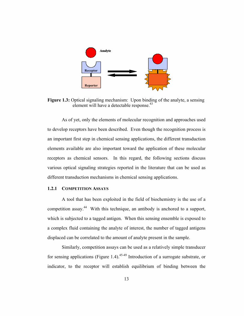
Figure 1.3: Optical signaling mechanism: Upon binding of the analyte, a sensing element will have a detectable response.43

As of yet, only the elements of molecular recognition and approaches used

to develop receptors have been described. Even though the recognition process is

an important first step in chemical sensing applications, the different transduction

elements available are also important toward the application of these molecular

receptors as chemical sensors. In this regard, the following sections discuss

various optical signaling strategies reported in the literature that can be used as

different transduction mechanisms in chemical sensing applications.

1.2.1 COMPETITION ASSAYS

A tool that has been exploited in the field of biochemistry is the use of a

competition assay.44 With this technique, an antibody is anchored to a support,

which is subjected to a tagged antigen. When this sensing ensemble is exposed to

a complex fluid containing the analyte of interest, the number of tagged antigens

displaced can be correlated to the amount of analyte present in the sample.

Similarly, competition assays can be used as a relatively simple transducer

for sensing applications (Figure 1.4).45-49 Introduction of a surrogate substrate, or

indicator, to the receptor will establish equilibrium of binding between the

Analyte

Receptor

Reporter

Analyte

Receptor

Reporter

14

indicator and the receptor and a receptor-indicator complex, resulting in a

particular optical response. Addition of the analyte of interest to the indicator-

receptor ensemble perturbs the equilibrium. The change in the established

equilibrium between the indicator and the receptor is dependent on the relative

degree of association between the analyte and the receptor.

Figure 1.4: A competition assay allows for the presence on an analyte to be detected upon displacement of an indicator molecule.

A popular method of developing an optical sensor uses the theme of

covalently attaching a transduction element to a receptor.50-53 A disadvantage to

this approach is that it introduces additional covalent architecture so that the

receptor can be converted into a sensor. This often requires more synthetic steps

which can be time-consuming and expensive, so utilizing competition assays

allows synthetic receptors to act as sensors without introducing additional

covalent architecture.

1.2.2 MICROENVIRONMENTAL CHANGE

One of the most common signaling strategies used in chemical sensing

involves using pH sensitive probes. There is a wide variety of pH indicators

available, but one of the first pH indicators to be used as a pH sensor was

+

Receptor

Indicator

Complex

CompetingAnalyte

+

Receptor

Indicator

Complex

CompetingAnalyte

15

fluorescein and it is often used to this day in studying biological systems.54,55

Fluorescein has a complex pH-dependent equilibrium (Figure 1.5) that undergoes

measurable colorimetric and fluorescent changes in the visible spectrum. These

optical changes are the result in the change of the protonation state of the phenols

and the carboxylate moieties on the xanthenene ring. As the pH of the solution

approaches the pKa of one of the phenols, there is an increase in the energy gap

between the excited state and the ground state that leads to an increase in the

quantum yield making fluorescein a very sensitive pH sensor.

Figure 1.5: The ionization state of the pH sensitive probe carboxyfluorescein.56

Setbacks to using fluorescein include susceptibility to photobleaching, a

pKa that is close to some biological systems where a probe with a higher pKa

would be preferable, and the fact that the cationic and neutral form are not

fluorescent, preventing use in low pH solutions or organic solvents.56 However,

like many of the molecular receptors mentioned earlier, chemists have modified

fluorescein to overcome some of these issues have created new probes with

chelating arms (chromoionophores) that allow for ion-selective pH sensors.

O OHHO

OH

OpKa = 2.1

O OHO

OH

O

NeutralCation

O OHO

Lactone

O

O

Monoanion

pKa = 4.2

O OHO

O

OpKa = 6.5

O OO

O

O

Dianion

O OHHO

OH

OpKa = 2.1

O OHO

OH

O

NeutralCation

O OHO

Lactone

O

O

Monoanion

pKa = 4.2

O OHO

O

OpKa = 6.5

O OO

O

O

Dianion

16

Another possible signaling motif exploits the hydrophobic effect. Ueno

and coworkers at the Tokyo Institute of Technology demonstrated that

fluorescently labeled cyclodextrins (CDs) could be used for chemical sensing.57-59

CDs are a group of torus-shaped cyclic D-glucose oligomers with the primary

hydroxyl groups of the sugar rings on the narrow rim of the CD cone (Figure 1.6).

These molecules are soluble in water and have shown the ability to shape-

selectively complex a variety of organic compounds including naphthalene and

pyrene in their hydrophobic cavity in aqueous solution.46,60,61

Figure 1.6: Schematic representation of the proposed sensor mechanism for dansyl modified CDs upon addition of guests.43

Sensing of these different guests by Ueno and coworkers was done by

competition assays.62 The CD molecules by themselves are silent in the UV-

Visible region, and detection of organic guests was accomplished using dansyl-

modified CDs.57 Dansyl is a solvatochromic dye that is sensitive to the

hydrophobicity of its microenvironment. As the guest binds to the CD, a

noticeable fluorescence signal modulation was detected. This fluorescence change

was rationalized as being the result of displacement of the dye from the CD cavity

as shown in Figure 1.6. Different guests resulted in variable decreases of the

Dansyl

Dansyl

Guest Guest

Narrow end of cone

Wide end of cone

Dansyl

Dansyl

Guest Guest

Dansyl

Dansyl

GuestGuest GuestGuest

Narrow end of cone

Wide end of cone

17

dansyl fluorescence demonstrating that dansyl-modified CDs are sensitive

chemosensors.

1.2.3 ENERGY TRANSFER

Energy transfer (ET) offers many opportunities for chemical sensing.

Specifically, fluorescence resonance energy transfer (FRET) has been described

as the radiationless transmission of energy from the initially excited donor

molecule to an acceptor molecule by resonance interaction of the oscillating

dipoles between the two chromophores.63 The efficiency of energy transfer is

dependent on the extent of spectral overlap of the emission spectrum of the donor

with the absorption spectrum of the acceptor (Figure 1.7), the quantum yield of

fluorescence of the donor, the relative orientation of the donor and acceptor

transition dipoles, and the distance between the two chromophores.63

Figure 1.7: Overlap integral (shaded area) for energy transfer from a donor molecule (dashed line) to an acceptor molecule (solid line).

Fluo

resc

ence

Wavelength (nm)

0

1.0

400 600300 500

0.5

DonorAcceptor

Fluo

resc

ence

Wavelength (nm)

0

1.0

400 600300 500

0.5

DonorAcceptor

18

The FRET method is frequently used to measure the distances between

two sites on a biological macromolecule.63 Utilizing energy-transfer in a sensing

scheme allows for the monitoring of the emission spectra of the probes upon

introduction of the analyte. This creates two modes of detection since one can

monitor emission intensities at two wavelengths (donor and acceptor). A

correlation could also be made between the ratio of the donor and acceptor

emission intensities and the analyte concentration, allowing the chemist to take

measurements that are independent of the inherent fluorophore concentration.

Other mechanisms for sensing include photoinduced electron-transfer

(PET). Generally, PET is used to quench the fluorescence of a fluorophore

attached to an amine on a cyclam or azocrown molecule capable of complexing

cations. The lone pair on the amine in the macrocycle is involved in the

quenching of the fluorophore while the macrocycle remains empty (no cation

present). However, when a cation is introduced into the host, the lone pair on the

amine participates in the binding of the analyte leaving the fluorophore to

generate a fluorescent signal.56 A significant advantage to this approach

compared to other signaling strategies is that the dynamic range of signal with

PET is larger due to the reduction of background signal (switching the probe from

“off” to “on”).

19

Scheme 1.3: Molecular structure of molecular thermometer created by Fabbrizzi utilizing PET as the sensing strategy.64

There are many examples of sensors using this signaling strategy for

complexing metal ions.65 In one case, a PET sensor was used to sense for the

physical property temperature. Fabbrizzi and coworkers constructed a molecular

thermometer (Scheme 1.3) using a naphthalene fluorophore segment covalently

linked to a tetraazamacrocycle.64 In acetonitrile (20°C), they found that the Ni(II)

complex 1.5 was present in 30% as a low spin species, while the high spin species

was present in 70%. The interconversion of 1.5 was found to be temperature

dependent, so the temperature was measured indirectly by calculating the ratio of

the two nickel spin state species. Fabbrizzi was able to record an increase in the

fluorescence emission for 1.5 over a temperature range of 27˚C to 65˚C, creating

a useful sensor capable of sensing the presence of Ni(II) and temperature.

1.3 Multi-Analyte Sensing

The development of compact array-based sensors has been largely

motivated by the demand for time-efficient and cost-effective analysis of complex

mixtures. As described in earlier sections of this chapter, chemical sensing has

NH

NH

HN

N

1.5

20

been achieved through the rational design of a receptor that has a high binding

affinity for a specific molecule (Figure 1.8A). This type of approach is

impractical for analyzing complex mixtures because it requires the synthesis of a

unique, highly selective sensor for each type of analyte to be detected.66 As a

result, trends in chemical sensing have shifted to the design of new materials and

devices that rely on a series of chemo- or biosensors such that recognition can be

achieved by the distinct pattern of responses produced from the combined effect

of all the sensors in the array (Figure 1.8B).

Figure 1.8: Shift in approaches taken for chemical sensing. (A) “Lock and Key” approach to host-guest systems. (B) Library of receptors approach.43

These approaches are advantageous because these devices can be

calibrated or “taught” to recognize a certain class of analytes with the help of

pattern recognition techniques67,68 For instance, if a similar analyte is introduced

A

B

“Lock and Key”

Library of Sensors

A

B

“Lock and Key”

Library of Sensors

21

to the array that it was not originally designed to recognize, the device could

result in an individualized response, thus signaling the presence of a new species.

Hence, the following section is dedicated to the discussion of sensor arrays

designed to analyze complex mixtures in vapor and solution phases inspired by

Nature’s approach to smell and taste.

1.3.1 SENSORY MIMICS

Many array-based sensors that are capable of sensing and identifying

multiple analytes in the vapor phase have been reported. These vapor sensors use

a variety of transduction schemes such as Surface Acoustic Wave (SAW),69-71

carbon black-polymer resistors,72,73 and conductive polymer74 transducers. These

structure sensors (referred to as “electronic noses”) mimic the mammalian sense

of smell and have demonstrated the ability to differentiate components within a

complex vapor mixture.75 The components of the mixture are classified based

upon the distinct pattern of responses detected over a collection of sensors in the

array.

A significant drawback of these types of devices is that they only apply to

analytes in the vapor phase. The need to develop sensors for applications

involving fluid analysis for areas such as environmental monitoring of waterways

or analyses of biologically relevant systems has spurred researchers into

developing sensing devices that mimic the mammalian sense of taste. The array-

based methodologies capable of fluid analysis that have emerged lately utilize a

range of detection schemes including microelectrodes,67,76 conducting

polymers,77-79 and fiber optic sensors.80

22

Likewise, at the University of Texas at Austin, the Anslyn and McDevitt

groups in collaboration with professors Jason Shear and Dean Neikirk, have

developed a device that allows for the simultaneous identification of multiple

analytes in solution.81,82 This device termed the “electronic tongue” consists of an

array of cross-linked copolymer microspheres (“taste buds”) that are chemically

modified with receptors or chemical indicators, and placed into a micromachined

platform as schematically represented in Figure 1.9. The detection platform

consists of a stereomicroscope fitted with a charged coupled device (CCD) that

yields red, green, and blue (RGB) signals for each sensor (bead) placed in

spatially addressable positions on the chip. The signaling mechanism used in the

“electronic tongue” is an observed color change by the CCD camera of the

sensing ensemble on the resin bead once it has been exposed to the analyte.

Analysis of the red, green, and blue light intensities from each of the sensors in

the array generates a pattern that can be used for analyte identification.

Figure 1.9: Schematic of micromachined chemosensor array (“electronic tongue”).43

UV Lamp

Micro-sensors

CCDUV Filter

Electronics Interface

Sensor Head Space

Light SourceUV Lamp

Micro-sensors

CCDUV Filter

Electronics Interface

Sensor Head Space

Light Source

23

An example of how RGB analysis is used to extract out information from

the sensors is shown in Figure 1.10. Figure 1.10A shows a digital picture taken

by the CCD camera of two resin beads composed of the same matrix that have

been chemically modified with acetic anhydride (top) which is used as a reference

sensor or “blank” and 5-carboxyfluorescein (bottom) which may be used to

indicate the pH of the solution. In the “blank” sensor case, the histograms of the

RGB intensities indicate that most of the light in each channel is passing through

the bead to be detected by the CCD camera (Figure 1.10B). However, in the

fluorescein sensor example, the RGB histogram shows a significant decrease in

the amount of light detected by the CCD camera in the blue channel relative to the

other two channels. This means that the ‘electronic tongue’ platform can be used

in the same fashion as a double-beam spectrophotometer where the ‘effective

absorbance’ of the fluorescein sensor can be calculated relative to the blank

sensor using Beer’s Law for the determination of hydronium ion concentration in

the solution being analyzed.

24

Figure 1.10: RGB Analysis of data generated by the multicomponent sensor array. (A) Color digital picture of a blank bead and a fluorescein anchored bead in the array. (B) Color histogram of each RGB channel for each bead in the array.

Sample delivery to the sensors is accomplished by a computer controlled

high-pressure liquid chromatography system that is connected to a flow cell. A

schematic of the flow cell is shown in Figure 1.11A. The silicon chip is situated

between two layers of Plexiglass which is clamped into an aluminum housing.

PEEK tubing is inserted into the Plexiglass layer which allows for fluid delivery

to enter from the top of the sensors and exit the flow cell from beneath the array.

The coupling of the fluid delivery system to the flow cell allows for specific

amounts of solutions to pass through the array of sensors for analysis.

BlankBeads

5-carboxy fluorescein

Beads

0 255

0 255

AB

BlankBeads

5-carboxy fluorescein

Beads

0 255

0 255

AB

25

Figure 1.11: Diagram of the fluid delivery system. (A) Schematic of flow cell. (B) Picture of instrument used for experiments composed of a FPLC fluid delivery system, CCD camera, flow cell, and a stereomicroscope.

With this arrangement of components, a very versatile instrument has

emerged that is capable of detecting cations, anions, solvents, sugars, and protein

structures such as biological cofactors and antibodies.83-85 The main components

-the resin beads, a silicon microchip, a flow cell, and a CCD camera- allow for

this analytical sensing device (Figure 1.11B) to be adapted for a range of

applications including environmental testing, liquid process control, and human

medicine. Specifically, the CCD detection affords highly sensitive and

simultaneous measurements of all the sensors in the array. Also, new sensors can

be readily synthesized incorporating a range of molecular building blocks

(including combinatorial libraries) using established solid phase synthesis

protocols. Finally, pattern recognition techniques can be applied to the

B FPLC

CCD

Microscope Stage

26

information generated by this platform so that the power of statistics can enable

this analytical detection device to solve more complex problems.

1.3.2 PATTERN RECOGNITION

Despite the recent attention that pattern recognition (PR) techniques have

received in the literature, the use of mathematical statistics in the handling and

interpretation of chemical data has been in practice long before the fieldname,

chemometrics, was coined in the early 1970’s.86 The methods applied to data sets

where measurements are recorded on many variables over a number of samples

are regularly called multivariate analysis (MVA) methods. The most common

methods used in chemical data handling are principle component analysis (PCA),

statistical discriminate analysis (SCA), soft independent modeling of class

analogy (SIMCA), cluster analysis through the k-nearest neighbor (k-NN), and

artificial neural networks (ANN).68

There are many detailed texts written describing the different MVA

methods available in chemistry.87-90 Since this dissertation only concerns the

application of just two PR methods, the discussion here is limited to PCA and

ANNs. Even though the basis for each approach to be discussed here has been

previously published, a more qualitative summary will be provided so that the

reader may appreciate the basic issues related to pattern recognition that will be

applied in later chapters in this dissertation.

PCA methods are commonly used to investigate variable (sensor)

interrelationships (correlations) among different samples. The main objective of

PCA is to simplify the dimensionality of a multivariate data set to a few

27

components so that the structure of the data may be interpreted more readily.89

For instance, consider a data set where n variables (sensors) give responses to m

samples as seen in Table 1.2. Here, the rows represent the responses of each

sensor for each sample and the columns signify the response of a single sensor

across all the samples.

Table 1.2: Example data for PCA where m is the number of samples tested, s represents a measurement response, and n is the number of sensors used in the study. [The sample examples are adenosine 5’-triphosphate (ATP) and adenosine 5’-triphosphate (ATP).]

In PCA, the sample responses obtained from a series of sensors are placed

into a matrix (n × m) where upon they are transformed into eigenvectors and

associated eigenvalues. In other words, PCA takes the correlated responses

(measured data) from each sensor (S1, S2,..Sn) and replaces them with linear

combinations of the measured responses (sATP1, sAMP1…smn) to generate derived

variables (eigenvectors) that are uncorrelated (unrelated functions of the

responses). This is done in order to generate a different dimension in the data set

which can be used to explain patterns in the data. These uncorrelated derived

variables are referred to as principal components (PCs).

S1 S2 . . . Sn

Samples ATP sATP1 sATP2 . . . sATPn

AMP sAMP1 sAMP2 . . . sAMPn

. . . . . . .

. . . . . . .m sm1 sm2 . . . smn

Sensors

28

If there are n response variables in the data set, then n components can be

derived, though, it is expected that most of the variability from the measured data

set can be accounted for within the first few PCs derived from the response

variables (sensors). Hence, the magnitude of the eigenvalue associated with the

eigenvector describes the importance (variability) of the newly derived variable.

Each PC is orthogonal (perpendicular) to the one that precedes it so that the

variance is maximized in each new component being generated: the first PC

accounts for the largest portion of variance in the data set and the second PC is

responsible for the second largest portion of variability and so forth. This allows

for these uncorrelated components to represent crucial features in the original data

set with minimal loss of information.88

Consider the following example illustrated in Figure 1.12 using two

variables (sensors) measuring two different samples (adenosine 5’-

monophosphate, AMP, and guanosine 5’-triphosphate, GTP) to create a two-

dimensional plot. Here, the distances between the responses of each sensor can

be used to describe the similarities and differences inherent within the data set

(Figure 1.12A). The first component axis (PC1) is drawn in the direction of the

maximum spread (variance) of data points (Figure 1.12B) and the second

component axis (PC2), perpendicular to PC1, is drawn in the direction of the

remaining variance not accounted for by PC1 (Figure 1.12C).

29

Figure 1.12: Principle component analysis of two variables upon exposure to two different samples. (A) The individual sensor response of two different sensors to three AMP and GTP samples. (B) A plot of the raw data with the first PC axis drawn in a dashed line. The coordinates of one sample relative to the original variable axes is shown in parenthesis. (C) The first two PC axes drawn in bold while the variable axes are shown in dashed lines. (D) The coordinates (or scores) of the same sample relative to the new PC axes is shown in parenthesis.

Now that a new dimensional space has been created by PC1 and PC2

(shown in solid lines in Figure 1.12C), coordinates of the samples (AMP and

GTP) relative to the new axis can be determined and are given “scores.” For

instance, the coordinate of one AMP sample relative to the variable axes is (0.8,

0.2) as shown in Figure 1.12B. However, the coordinates of this same sample

A Variable 2(Sensor #2)

Variable 1(Sensor #1)

GTP

AMP



New Axis 1(PC 1)

B

GTP

AMP



New Axis 1(PC 1)

C

GTP

AMP

New Axis 2(PC 2)

(0.8, 0.2)



New Axis 1(PC 1)

New Axis 2(PC 2)

D

GTP

AMP

(0.5, -0.5)

30

relative to the new PC axes is (0.5, -0.5) as shown in Figure 1.12D. These new

coordinates (scores) can then be plotted with respect to the PCs and used to

describe the correlation between samples. An example of this kind of plot,

termed a score plot, is shown in Figure 1.13. A score plot allows for the trends in

the data to be visualized in a simple way. Samples with similar PC scores

indicate that they may have comparable characteristics. For example, in Figure

1.13 the clustering of the ATP and GTP samples can be explained by the fact that

they are triphosphates and more similar in structure than the monophosphate

samples, AMP and pyrophosphate, that cluster in a different region on the score

plot.

Figure 1.13: PCA score plot showing clustering of different types of phosphates (♦ATP, ▲GTP, ●AMP, ■Pyrophosphate or PP) with one of the AMP samples coordinates drawn in dashed lines to each PC axis.

Principle Component #1(Largest % Variance)

Prin

cipl

e C

ompo

nent

#2

(Nex

t Lar

gest

% V

aria

nce)

GTP

AMPPP

1.0-1.0

0.0

1.0

-1.0

0.5ATP

-0.5

Principle Component #1(Largest % Variance)

Prin

cipl

e C

ompo

nent

#2

(Nex

t Lar

gest

% V

aria

nce)

GTP

AMPPP

1.0-1.0

0.0

1.0

-1.0

0.5ATP

-0.5

31

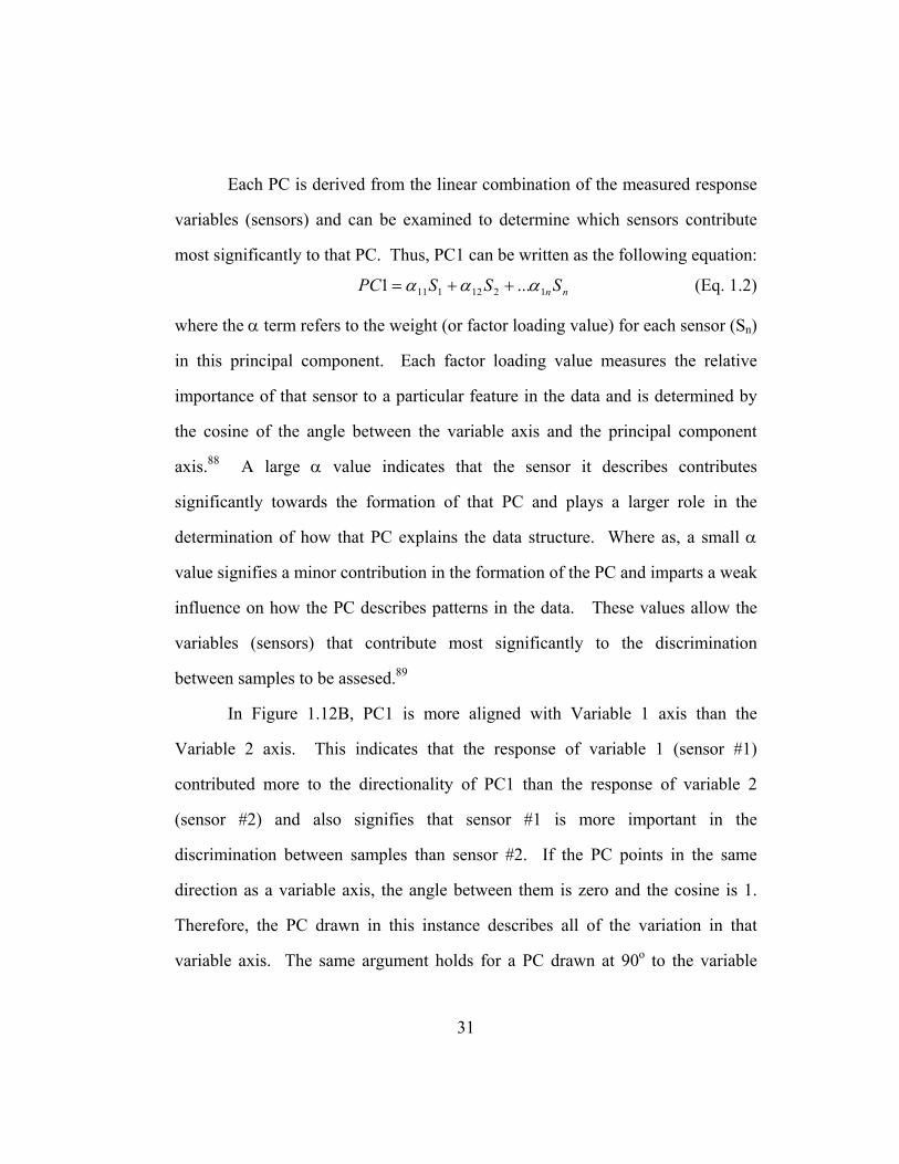
Each PC is derived from the linear combination of the measured response

variables (sensors) and can be examined to determine which sensors contribute

most significantly to that PC. Thus, PC1 can be written as the following equation:

nn SSSPC 1212111 ...1 ααα ++= (Eq. 1.2)

where the α term refers to the weight (or factor loading value) for each sensor (Sn)

in this principal component. Each factor loading value measures the relative

importance of that sensor to a particular feature in the data and is determined by

the cosine of the angle between the variable axis and the principal component

axis.88 A large α value indicates that the sensor it describes contributes

significantly towards the formation of that PC and plays a larger role in the

determination of how that PC explains the data structure. Where as, a small α

value signifies a minor contribution in the formation of the PC and imparts a weak

influence on how the PC describes patterns in the data. These values allow the

variables (sensors) that contribute most significantly to the discrimination

between samples to be assesed.89

In Figure 1.12B, PC1 is more aligned with Variable 1 axis than the

Variable 2 axis. This indicates that the response of variable 1 (sensor #1)

contributed more to the directionality of PC1 than the response of variable 2

(sensor #2) and also signifies that sensor #1 is more important in the

discrimination between samples than sensor #2. If the PC points in the same

direction as a variable axis, the angle between them is zero and the cosine is 1.

Therefore, the PC drawn in this instance describes all of the variation in that

variable axis. The same argument holds for a PC drawn at 90o to the variable

32

axis. The cosine of 90o is zero, indicating that none of the response variation is

contained in the PC axis. To summarize, similar factor loading values indicate

that the variables (sensors) responded in a similar fashion to the samples and may

indicate important relationships among the sensors.

The example given above only represents the basic idea of PCA and how

it can be applied in a two-variable case. PCA can be extended to multiple

variables where the computations are more involved and require the use of a

statistical analysis software program. This makes PCA a powerful tool for

chemical applications where the basic principle of data reduction allows chemists

to explore their own data in a more simplified form.

Another frequently mentioned pattern recognition technique used for

applications in chemistry is an ANN. The ANNs considered here are the feed-

forward multilayer perceptron (FF-MLP) ANNs that have often proven to be

useful for the analysis of data from sensor arrays.68 The objective for ANN

analysis is to generate a model from multivariate data sets and create criterion

from which a successful network response will reveal the “best fit” answer to any

input.

The basic architecture of a FF-MLP neural network consists of several

layers containing a number of units, or neurons, where the data is processed and

passed onto subsequent units located in the next layer. A general schematic of a

single neuron is shown in Figure 1.14. In a FF-MLP, each neuron produces an

output as a function of its input which may be data from the sensor array or the

output of a previous neuron. The information that is received in each unit is

33

compiled by first applying a series of weights (wij) and biases to each input value

(Ii) and then subjecting each value to a transfer function that is ultimately

presented as the output value (Outj).87 The application of weights and biases to

each input value allows for the network to adjust or learn its training data.

Figure 1.14: Operation of a single “neuron” or input unit in an FF-MLP ANN. A summation of all input signals are subjected to a weight (Wnj) and transfer function before sent on as an output (Outj) to the next “neuron.”

The network is often organized into three layers as shown in the diagram

below (Figure 1.15). The input layer usually contains a number of neurons (often

equal to the number of sensors) that accept the external data and perform no

calculations on the data but only represent input values.90 The output layer

typically contains neurons for each value to be predicted by the network. The

intermediate (hidden) layers are situated between the input layer and the output

layer where the number of hidden layers can be varied and are determined

experimentally. The neurons in each layer are all connected to each other (as

shown in Figure 1.15) and this allows the network to solve nonlinear problems.

Inpu

t OutputSumFunction

TransferFunction

W1j

W2j

W3j

I1

I3

I2 Outj

34

Figure 1.15: A diagram of a three layered FF-MLP ANN. The ANN is composed of an input layer, a variable number of hidden layers, and an output layer.

In order to generate an answer from the network, the network must be

trained by iteratively changing the weights and biases using a back propagation

algorithm. Individual data streams with known output values are entered into the

network and the weights and biases are changed so that the error between the true

value and the predicted (network) value are minimized. The training errors

reported by the network need to be evaluated carefully since the network is

capable of being overtrained (the network memorizes the data and has no

predictive behavior).68 If high errors persist, changing parameters like the

number of layers, neurons, or data formats initially imputed into the input layer

may improve the performance of the network.

Once the network has been trained, validating the networks ability to

predict values based on the relationships learned from the data is done by omitting

a single data point from the training data set. Training of the network is carried

out again, and then the left out point is imputed as an unknown sample. If the

error associated with this removed data point is close to the training error, the

Hidden layer

Output layer

Input layer

Hidden layer

Output layer

Input layer

35

network model is said to be valid. Ultimately, the error associated with a “real”

unknown sample is the best way to gage the networks ability.

A common attribute for PCA and ANN analysis is that they are both used

to understand relationships between data sets. Yet, the significant difference lies

in the approach with which the data is inputted for each analysis. PCA is

considered an unsupervised learning technique meaning that the relationship

between the data will evolve from the calculations without using membership

classification beforehand. On the other hand, ANN analysis is used to create a

model based on data sets with known output values for classifying or quantifying

future unknown samples. These methods sometimes experience limitations with

their sensitivity to analyzing samples outside their training set or sample volume

giving erroneous results.68,90 However, both of these methods possess distinctive

advantages for analyzing multivariate data sets in various settings and ultimately

provide a chemist with the means to quickly extract distinctive patterns from large

volumes of data found in real-world problems.

1.4 Outlook

The field of chemical sensing is a science that bridges the chemical,

biological, engineering, and material sciences with foundations in chemistry

spanning organic, analytical, physical, and inorganic chemistry. Therefore, the

development of sensors capable of detecting the presence of analytes requires a

multifaceted approach.

With the many approaches taken by chemists to develop sensors,

numerous signaling strategies have emerged in the literature towards the detection

36

of anaytes. Even though many of these signal transduction mechanisms have

been explored in the Anslyn and McDevitt research groups, the indicator-

displacement assay has often proven to be a successful strategy. Chapter 2

focuses on the application of an indicator-displacement assay with a synthetic

host to quantitate the amount of citrate in commercial beverages. Also,

application of an ANN with the same two-component sensing ensemble allows

for the determination of citrate and calcium concentrations in flavored vodkas.

Investigators, with a large knowledge base to draw from concerning

molecular recognition and host design, are now able take chemical sensing into an

area ripe for cultivation. This new emerging science couples the concepts of

molecular sensing with array-based platforms so that sensing of multiple analytes

can be accomplished. Trends are now shifting towards utilizing an array of

differential sensors responsive to various classes of analytes instead of using

sensors specifically designed to target one analyte. Combining the signals from

all the sensors in the array generates a fingerprint response that is unique to the

composition of the mixture being analyzed. In Chapter 3 and Chapter 4, this

concept is employed by coupling the principles of supramolecular chemistry and

pattern recognition to create new sensing protocols for the analysis of nucleotide

phosphates and phosphonates in aqueous solutions.

A novel optically-based sensor array platform was described in Section

1.3.1 with versatile components that can be modified for different applications

evaluating complex mixtures. We expect that by expanding this “lab-on-a-chip”

technology to incorporate differential sensors and pattern recognition, analysis of

37

various classes of analytes within this platform has the potential to be a viable

sensing device for biochemical and chemical warfare degradation products.

Attributes such as high sensitivity, low detection limits, reduction of false

positives, short assay times, and minimal consumption of reagents have been

demonstrated in our previous reports utilizing this detection platform and show

promise for the incorporation of the sensing strategies described herein.

38

CHAPTER 2: COMPETITIVE INDICATOR METHODS USED FOR THE ANALYSIS OF CITRATE AND CALCIUM IN

BEVERAGES

2.0 Introduction

As described in Chapter 1, many investigations have been carried out to

develop single analyte molecular sensors. The application of these molecular

sensors requires the presence of a reporter molecule capable of signaling the

binding of the analyte to the host. The two most reoccurring signal transduction

themes are the covalent attachment of the signaling molecule to the host or

competition between the target analyte and the signaling molecule.66

Competition assays are the focus of this chapter. Specifically, a

competitive indicator method for studying host:guest complexes is extended to

systems forming I:H, I:H2, and A:H complexes of indicator (I), host (H) and

competing analyte (A). Methods are applied to complexes of a synthetic organic

host (2.1) with commercially available indicators xylenol orange (2.4) and

methylthymol blue (2.5). Utilizing complexometric indicators results in an

observable shift in λmax upon binding of the analyte and, subsequently may

enhance the sensitivity of these competition assays due to a larger dynamic range

in the change of absorption. The binding constants for the association between

I:H, I:H2, and A:H are reported. These sensing ensembles have been tested in

competitive media. Competition assays using UV-Vis spectroscopy and each

39

host-indicator ensemble allowed for the determination of citrate in various

beverages.

Finally, pattern recognition algorithms were applied to a two-component

sensing ensemble to differentiate among solutions containing various

concentrations of calcium and citrate ions. The concentrations of calcium and

citrate in various flavored vodkas were determined through artificial neural

network (ANN) analysis. Herein, the new developments are summarized and the

utility of this method is described in the context of the analysis of citrate and

calcium ion in citrus beverages using a synthetic receptor paired with an optical

signaling molecule and ANN.

2.1 Development of a Host for Citrate

The Anslyn group has used indicator-displacement assays with a series of

synthetic organic hosts in order to detect various analytes.91-95 In one system, a

receptor for citrate was developed that is selective for this tris-carboxylate

compound even in the presence of other common carboxylates.92 The choice of

citrate as the target analyte was due to the potential commercial interest in a

sensor for citrate by beverage bottling companies.

The receptor (or host) 2.1 consists of a 2,4,6-triethylbenzene core

substituted with guanidinium moieties in the 1, 3, and 5 positions. Each adjacent

substituent on the benzene ring alternates above and below the plane of the ring to

minimize steric interactions, causing the guanidiniums to lay on one face of the

benzene ring.96 Receptors containing similar structures to 2.1 have demonstrated

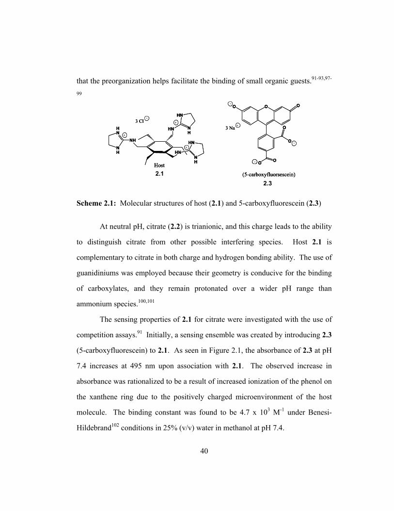
40

that the preorganization helps facilitate the binding of small organic guests.91-93,97-

99

Scheme 2.1: Molecular structures of host (2.1) and 5-carboxyfluorescein (2.3)

At neutral pH, citrate (2.2) is trianionic, and this charge leads to the ability

to distinguish citrate from other possible interfering species. Host 2.1 is

complementary to citrate in both charge and hydrogen bonding ability. The use of

guanidiniums was employed because their geometry is conducive for the binding

of carboxylates, and they remain protonated over a wider pH range than

ammonium species.100,101

The sensing properties of 2.1 for citrate were investigated with the use of

competition assays.91 Initially, a sensing ensemble was created by introducing 2.3

(5-carboxyfluorescein) to 2.1. As seen in Figure 2.1, the absorbance of 2.3 at pH

7.4 increases at 495 nm upon association with 2.1. The observed increase in

absorbance was rationalized to be a result of increased ionization of the phenol on

the xanthene ring due to the positively charged microenvironment of the host

molecule. The binding constant was found to be 4.7 x 103 M-1 under Benesi-

Hildebrand102 conditions in 25% (v/v) water in methanol at pH 7.4.

HN

NH

3 ClHN

NH

HN

HN

NH

NH

HN

O OO

O

O

-

-

- O O

3 Na +

Host1 (5-carboxyfluorsescein)

3

-

+

+

+

2.12.3

HN

NH

3 ClHN

NH

HN

HN

NH

NH

HN

O OO

O

O

-

-

- O O

3 Na +


3

-

+

+

+

HN

NH

3 ClHN

NH

HN

HN

NH

NH

HN

O OO

O

O

-

-

- O O

3 Na +


3

-

+

+

+

2.12.3

41

Figure 2.1: UV-Vis spectra of 2.3 in 25% (v/v) water in methanol with 5 mM HEPES buffer at pH 7.4. Addition of 2.1 to a solution of 2.3 at constant concentration (14 µM) causes an increase in absorbance at 495 nm (arrows indicate the direction of change in the absorbance intensity).92

Addition of sodium citrate to the indicator-host complex causes a decrease

in the observed absorbance of fluorescein at 495 nm (Figure 2.2). It was reasoned

that the 5-carboxyfluorescein (2.3) was expelled from the binding pocket due to

the higher binding affinity of citrate with 2.1. A binding constant for citrate with

2.1 was found to be 2.9 x 105 M-1 in this solvent system. Significantly reduced

affinities were found for succinate, glutarate (both valued close to 2 x 102 M-1)

and acetate (less than 10 M-1).92

0.45

0.05

Abs

orba

nce

λ (nm)420 520

0.45

0.05

Abs

orba

nce

λ (nm)420420 520520

42

Figure 2.2: UV-Vis spectra of 2.3 in 25% (v/v) water in methanol with 5 mM HEPES buffer at pH 7.4. Addition of 2.2 to the sensing ensemble 2.1:2.3 at constant concentration (75 µM 2.1, 14 µM 2.3) causes a decrease in absorbance at 495 nm (arrows indicate the direction of change in the absorbance intensity).92

A practical use of an ensemble of 2.1 and 2.3 was demonstrated by

evaluating the amount of citrate in various complex mixtures. Calibration curves

were generated for varying amounts of citrate from the absorbance data obtained

from the citrate competition assay. With these plots, aliquots of different citrus

beverages were added to a solution of the 2.1:2.3 complex and the absorbance

recorded.91 This allowed for the analysis of citrate in commercially available

beverages and further demonstrated that 2.1 possess selectivity for citrate in the

presence of other competing analytes.

Although this assay was successful, three improvements were desired.

One was a λmax shift, which creates a color change and therefore a larger dynamic

range in the change in absorbance. Another goal was to show that many

commercially available indicators could be used with the same receptor. This

gives chemists larger latitude in the ability to choose indicators for displacement

420 520λ (nm)

0.45

0.05

Abs

orba

nce

420 520λ (nm)

0.45

0.05

Abs

orba

nce

43

assays using synthetic receptors. Third, the multi-analyte sensing capabilities of

these sensing ensembles are demonstrated via application of ANN analysis. To

this end, competition assays are employed with standard spectrophotometer to

sense for calcium and citrate in various beverages.

2.2 Binding Studies

2.2.1 SELECTION OF THE INDICATORS AND EXPERIMENTAL CONDITIONS

Using competition assays for the evaluation of analytes in solution

requires that the indicator form a complex with the ligand or host molecule.

Another requirement is that the absorption spectra of the complexed form differ

significantly from the absorption spectra of the uncomplexed form. The choice of

indicators in this study was guided by two factors. First, the binding of

carboxylates with guanidinium groups imbedded in aminoimidazoline groups is

well precedented,91-95 and therefore the use of complexometric indicators

possessing carboxylates in their structure were explored. Second, we chose

indicators that change color as a function of pH, thereby expecting similar color

changes within the microenvironment of the host. Xylenol orange (2.4) and

methylthymol blue (2.5) were chosen as the indicators for the purposes of our

studies.

At neutral pH, metal cations typically coordinate to the iminiodiacetic acid

residues and the auxochromic phenol oxygen of 2.4 and 2.5 inducing a shift in the

λmax.103-106 We expected that complexation of 2.4 or 2.5 to 2.1 would result in a

similar color change of the indicator due to increased ionization of the phenols.

The structural features of these two indicators (I) clearly show that there are two

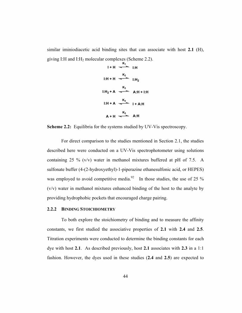
44

similar iminiodiacetic acid binding sites that can associate with host 2.1 (H),

giving I:H and I:H2 molecular complexes (Scheme 2.2).

Scheme 2.2: Equilibria for the systems studied by UV-Vis spectroscopy.

For direct comparison to the studies mentioned in Section 2.1, the studies

described here were conducted on a UV-Vis spectrophotometer using solutions

containing 25 % (v/v) water in methanol mixtures buffered at pH of 7.5. A

sulfonate buffer (4-(2-hydroxyethyl)-1-piperazine ethanesulfonic acid, or HEPES)

was employed to avoid competitive media.92 In those studies, the use of 25 %

(v/v) water in methanol mixtures enhanced binding of the host to the analyte by

providing hydrophobic pockets that encouraged charge pairing.

2.2.2 BINDING STOICHIOMETRY

To both explore the stoichiometry of binding and to measure the affinity

constants, we first studied the associative properties of 2.1 with 2.4 and 2.5.

Titration experiments were conducted to determine the binding constants for each

dye with host 2.1. As described previously, host 2.1 associates with 2.3 in a 1:1

fashion. However, the dyes used in these studies (2.4 and 2.5) are expected to

I + H I:HK1

I:H2 + AK3

A:H + I:H

I:H + HK2

I:H2

I:H + AK4

I + A:H

A + H A:HK5

45

associate with the host giving I:H and I:H2 complexes. This expectation is borne

out by the lack of sharp isosbestic points.

2.2.3 BINDING DATA

The absorbance of 2.4 (Figure 2.3) at pH 7.5 increases at 577 nm upon

association with 2.1, while the absorbance decreases at 445 nm (solutions change

from an orange color to a pink-red). Similarly, the absorbance of 2.5 (Figure 2.4)

at pH 7.5 increases at 607 nm upon addition of 2.1 with a decrease in absorbance

at 454 nm (solutions change from a light yellow to a cobalt blue). It is reasoned

that the binding of the positively-charged host molecule to the carboxylates on the

indicator would lower the pKa of the indicator phenol groups due to the positive

microenvironment present in the host. The observed color changes correlate with

the indicators acting as if they are in a more basic microenvironment. The

increased ionization state of the indicators is due to the positive charges on the

receptor, and the increased electron density on the auxochromic oxygen leads to

the observed λmax changes.

46

Figure 2.3: UV-Vis spectra of 2.4 in 25% (v/v) water in methanol with 10 mM HEPES buffer at pH 7.5. Addition of 2.1 to a solution of 2.4 at constant concentration (55 µM) causes and increase of absorbance at 577 nm and a decrease in absorbance at 445 nm (arrows indicate the direction of change in the absorbance intensity).

In Figures 2.3 and 2.4, a large change in absorbance was observed with the

addition of 2.1 to each indicator. For instance, the percent difference in

absorbance at 577 nm between the absorbance of the dye in solution and the

absorbance of the 2.4:2.1 complex in Figure 2.3 was 238%, and the percent

difference in absorbance at 607 nm in Figure 2.4 was calculated to be 521%. This

is a significantly larger dynamic range in change in signal compared to the 73%

increase in signal observed with the addition of 2.1 to 5-carboxyfluorescein

(Figure 2.1). The dramatic increase in signal in both cases with indicators 2.4 and

2.5 is attributed to their ability to shift their λmax upon complexation with host 2.1.

Abs

orba

nce

0

1.8

1.0

0.4

λ (nm)400 600500

Abs

orba

nce

0

1.8

1.0

0.4

λ (nm)400 600500

47

Figure 2.4: UV-Vis spectra of 2.5 in 25% (v/v) water in methanol with 10 mM HEPES buffer at pH 7.5. Addition of 2.1 to a solution of 2.5 at constant concentration (55 mM) causes an increase in absorbance at 607 nm and a decrease in absorbance at 454 nm (arrows indicate the direction of change in the absorbance intensity).

2.2.4 DERIVATION OF BINDING EQUATIONS

The system studied contained 1:1 (I:H) and 1:2 (I:H2) complexes of

indicator (I) with host (H). The following Eqs. 2.1 and 2.2 describe the

interactions between host (2.1) and indicator (2.4 or 2.5).

I + H IH Eq. 2.1

IH + H IH2 Eq. 2.2

The absorbance of the solution of xylenol orange (Ao) prior to the addition

of host is described by Beer's Law, Eq. 2.3;

][IbAo ⋅⋅= ε Eq. 2.3

0

1.0

0.5

0.2A

bsor

banc

e

λ (nm)

0

1.0

0.5

0.2A

bsor

banc

e

λ (nm)

48

where ε is the molar absorptivity of the indicator, b is the path length of light

through the sample solution, and [I] is the concentration of the indicator present.

After the addition of host, the equation for describing all the absorbing

species (A) in the solution becomes:

][][][][ 22

IHbIHbHbIbA IHIHiHiI ⋅⋅+⋅⋅+⋅⋅+⋅⋅= εεεε Eq. 2.4

where [Ii] and [Hi] represent the concentration of the free indicator and host in

solution, respectively, and [IH] and [IH2] are the concentrations of any complexes

that may form between the them.

The total concentration of each species (IT and HT) is depicted by the mass

balance equations for both the indicator and the host molecule.

][][][][ 2IHIHII iT ++= Eq. 2.5

][2][][][ 2IHIHHH iT ⋅++= Eq. 2.6

Solving Eq. 2.5 and Eq. 2.6 for [Ii] and [Hi], respectively and

incorporating the expressions into equation 2.4 gives Eq. 2.7.

( ) ( )

][][][2][][][][][

2

22

2IHbIHb

IHIHHbIHIHIbA

IHIH

THTI

⋅⋅+⋅⋅+⋅−−⋅+−−⋅=

εεεε

Eq. 2.7

Since the host has no absorbance at the wavelength that is being

monitored, the εH term becomes zero. Upon eliminating this term and combining

like terms, the equation becomes:

][)(][)(][ 22IHbIHbIbA IIHIIHTI ⋅⋅−+⋅⋅−+⋅⋅= εεεεε Eq. 2.8

49

Dividing the path length from each side of the equation gives:

][][][ 221 IHIHIbA

TI ⋅∆+⋅∆+⋅= εεε Eq. 2.9

where ∆ε1 = εIH - εI and ∆ε2 = εIH2 - εI. The equilibrium constants in this system

are given by:

][][][

1ii IH

IHK⋅

= Eq. 2.10

][][][ 2

2iHIH

IHK⋅

= Eq. 2.11

Rearrangement of these expressions and substitution into Eq. 2.9 gives the

result:

( ) ( )][][][][][ 212211 iiiiTI IHKKIHKI

bA

⋅⋅⋅⋅∆+⋅⋅⋅∆+⋅= εεε Eq. 2.12

Since [IT] is held constant, the absorbance of the indicator prior to the first

addition of host (A0) is subtracted from each subsequent absorbance reading after

the addition of the host (Ai). This results leads to the εI term dropping out of the

expression.

( ) ( )][][][][ 212211 iiii IHKKIHK

bA

⋅⋅⋅⋅∆+⋅⋅⋅∆=∆ εε Eq. 2.13

As mentioned earlier, the equilibrium expressions can be rewritten as:

][][][ 1 ii IHKIH ⋅⋅= Eq. 2.14

][][][ 222 ii IHKIH ⋅⋅= Eq. 2.15

50

Using these values and substituting into the mass balance Eq. 2.5 and

solving for [Ii] will give the equation:

2121 ][][1

][][

ii

Ti HKKHK

II

⋅⋅+⋅+= Eq. 2.16

Combining Eq. 2.16 with Eq. 2.13 results in the equation for the binding

isotherm for a 1:2 [I:H2] complex.

( ) ( )

2121

2211

][][1][][][

ii

iTi

HKKHKHKIHK

bA

⋅+⋅+⋅⋅∆+∆⋅⋅⋅

=∆ εε

Eq. 2.17

The term [HT] is a value that can be determined experimentally, where as,

the concentration of free host, [Hi], cannot be measured directly. This creates the

need to relate [Hi] to [HT] and can be accomplished by substituting Eq. 2.16 into

the rearranged form of Eq. 2.14, giving Eq. 2.18.

2121

1

][][1][][

][ii

Ti

HKKHKIHK

IH⋅⋅+⋅+

⋅⋅= Eq. 2.18

Now, substitute Eq. 2.18 into the mass balance equation for [HT]. This

relates the total concentration of host to the concentration of free host in solution.

⋅⋅+⋅+

⋅⋅⋅⋅+

⋅⋅+⋅+

⋅⋅+= 2

121

212

2121

1

][][1][][2

][][1][][

][][ii

iT

ii

TiiT HKKHK

HIKKHKKHK

IHKHH

Eq. 2.19

51

Rearrangement of Eq. 2.19 in order to solve for [Hi] gives the following

cubic expression:

( )

( ) 0][][1][][][1][][2][

11

2221

321

=−⋅+⋅−⋅+⋅+⋅−⋅⋅+⋅⋅

TiTT

iTTi

HHHKIKHHKIKKHKK

Eq. 2.20

Using Eq. 2.17 and Eq. 2.20, it is possible to extract a binding constant

from a plot of the change in absorbance (∆A) versus the total concentration of

indicator [IT].

2.2.5 CURVE FITTING ANALYSIS

As shown in Figure 2.5 A and B, addition of citrate to the indicator-host

complexes causes a reverse in the observed absorbance of both xylenol orange

and methylthymol blue at 577 nm and 607 nm, respectively. As seen with the

citrate assay employing 5-carboxyfluorescein, the indicator is expelled from the

binding pocket due to the higher binding affinity of 2.1 with citrate (Scheme 2.3).

52

Figure 2.5: UV-Vis spectra of 2.4 and 2.5 in 25% (v/v) water in methanol with 10 mM HEPES buffer at pH 7.5. (A) Addition of 2.2 to a solution of 2.4:2.1 at constant concentration (55 µM 2.4, 1.13 mM 2.1) causes a decrease in absorbance at 577 nm and an increase in absorbance at 445 nm. (B) Addition of 2.2 to a solution of 2.5:2.1 at constant concentration (55 µM 2.5, 1.13 mM 2.1) causes a decrease in absorbance at 607 nm and an increase of absorbance at 454 nm (arrows indicate the direction of change in the absorbance intensity)

Extraction of the binding constants, K1 and K2, for the association between

each indicator molecule and the host is complicated. There are four variables:

two binding constants (K1 and K2), and two different extinction coefficients (1:1

indicator-host complex, and 1:2 indicator-host complex). A method for

determining 1:1 and 1:2 binding constants from optical spectroscopy data has

been discussed.45-49,107

400

λ (nm)

600500

Abs

orba

nce

0

1.8

1.0

0.4

A.

λ (nm)

0400 600500

1.0

0.5

0.2

Abs

orba

nce

B.

400

λ (nm)

600500

Abs

orba

nce

0

1.8

1.0

0.4

400

λ (nm)

600500

Abs

orba

nce

0

1.8

1.0

0.4

A.

λ (nm)

0400 600500

1.0

0.5

0.2

Abs

orba

nce

λ (nm)

0400 600500

1.0

0.5

0.2

Abs

orba

nce

0400 600500

1.0

0.5

0.2

Abs

orba

nce

B.

53

Scheme 2.3: Molecular structures of the host (2.1) and indicators (2.4 and 2.5) used to sense for citrate.

The program Mathematica 3.0 was used to solve Eq. 2.20 for [Hi] with

multiple values of [HT] and several initial estimates of K1, K2, ∆ε1, and ∆ε2. Each

value for [Hi] is substituted into Eq. 2.17. The fit of Eq. 2.17 to the data is

accomplished by prompting the user for initial estimates for K1, K2, ∆ε1, and ∆ε2.

The model equation (Eq. 2.17) is overlaid graphically with the experimental

values obtained for ∆A/b (the path length is 1.00 cm) and [HT]. The values K1,

K2, ∆ε1, and ∆ε2 are modified and the data replotted until the best fit between

experimental data and the model is visually achieved, as shown in Figure 2.6.

HN

HN

HN

NH

HN

HN

NH

NH

HN3 Cl

HN

HN

HN

NH

HN

HN

NH

NH

HNHO

O

O

O

O O

O

HOO

O

O

O O

O

SO3

O

CH2N(CH2COO )2

CH2N(CH2COO )2

OH

3 Na

+

+

+

-

-

-

+

-

-

-

- -+

+

+Indicator (I)

OH

O

SO3

( OOCH2C)2N

N(CH2COO )2

3 Na

-

-

-

+

Host (H)1

Citrate (A)2

A:H Complex

I1 Xylenol Orange4

I2 Methylthymol Blue5

-

-

2.1

2.4 2.5

2.2

HN

HN

HN

NH

HN

HN

NH

NH

HN3 Cl

HN

HN

HN

NH

HN

HN

NH

NH

HNHO

O

O

O

O O

O

HOO

O

O

O O

O

SO3

O

CH2N(CH2COO )2

CH2N(CH2COO )2

OH

3 Na

+

+

+

-

-

-

+

-

-

-

- -+

+

+Indicator (I)

OH

O

SO3

( OOCH2C)2N

N(CH2COO )2

3 Na

-

-

-

+

Host (H)1

Citrate (A)2

A:H Complex

I1 Xylenol Orange4

I2 Methylthymol Blue5

-

-

2.1

2.4 2.5

2.2

54

Figure 2.6: Theoretical fit (-) of Eq. 2.17 to the experimental data (○) obtained from ∆A as a function of the addition of 2.1 to each indicator. (A) Isotherm plot for addition of 2.1 to 2.4 (λ = 577nm). (B) Isotherm plot for the addition of 2.1 to 2.5 (λ = 607nm).

The binding constants determined for the 2.4:2.1 molecular complex were

K1= 7.05 x 103 M-1 and K2 = 2.08 x 103 M-1. The affinity constants determined

for the 2.5:2.1 molecular complex were K1= 3.95 x 103 M-1 and K2 = 1.10 x 102

M-1. These results show that xylenol orange has a larger affinity for 2.1 than

methylthymol blue. This observation may be attributed to the presence of the

isopropyl groups on methythymol blue as opposed to the methyl groups at the

0

Del

ta A

BS (5

77 n

m)

0.2

0.8

1.4 A.

0.0002 0.0005 0.0008

[Host] M

B.

Del

taAB

S (6

07 n

m)

0.1

0.5

0.9

0 0.0004 0.00140.0008

0

Del

ta A

BS (5

77 n

m)

0.2

0.8

1.4 A.

0.0002 0.0005 0.0008

[Host] M

B.

Del

taAB

S (6

07 n

m)

0.1

0.5

0.9

0 0.0004 0.00140.0008

55

corresponding positions in the xylenol orange structure. The added steric bulk on

2.5 could hinder access of 2.1 to the indicator binding sites, resulting in slightly

smaller binding constant values.

The equilibrium equations given in Scheme 2.2 for the displacement of the

indicators upon addition of 2.2 are as follows:

][][][][

23 AIH

IHAHK⋅

⋅= Eq. 2.21

][][][][

4 AIHIAHK

⋅⋅

= Eq. 2.22

The equilibrium expression for the association of host 1 with citrate is:

][][][

5 AHAHK

⋅= Eq. 2.23

Hence, the displacement constants K3 and K4 can be determined by using

the following relationships:

2

53 K

KK = Eq. 2.24

1

54 K

KK = Eq. 2.25

With xylenol orange, the values for K3 and K4 obtained from Eqs. 2.24

and 2.25 are 1.39 x 102 M-1 and 41.1 M-1, respectively. In the methylthymol blue

studies, the values for K3 and K4 obtained from Eqs. 2.24 and 2.25 are 2.64 x 103

56

M-1 and 73.4 M-1, respectively. These values for K3 and K4 were calculated using

the binding constant (K5) presented earlier.91 It was reasoned previously that the

association constants for methylthymol blue to 2.1 were smaller than the

corresponding K1 and K2 values for xylenol orange due to added steric bulk on the

methylthymol blue structure. It follows that the displacement constants for

xylenol orange upon introduction of citrate are smaller than the corresponding K3

and K4 values for methylthymol blue because of the stronger association of the

2.4:2.1 complex. The association of the 2.5:2.1 complex is slightly weaker than

the 2.4:2.1 complex and therefore the 2.5:2.1 complex will disassociate more

readily in order for the 2.1:2.2 complex to form upon introduction of citrate.

2.3 Beverage Analysis

2.3.1 CITRATE IN BEVERAGES

In order to demonstrate that these sensing systems can be employed for

practical uses, calibration curves were generated for citrate (Figure 2.7) in order to

evaluate various citrus beverages. The determination of citrate in various

beverages was performed by UV-Vis spectroscopy in 10 mM HEPES buffer at pH

7.5 with a 25% (v/v) water in methanol mixture.

57

Figure 2.7: Calibration curves used for the citrate assay (25% (v/v) water in methanol with 10 mM HEPES buffer at pH 7.5). (A) UV-Vis calibration curve using 2.4 at the indicator (55 µM 2.4, 1.13 mM 2.1, λ = 577 nm). (B) UV-Vis calibration curve using 2.5 at the indicator (55 µM 2.5, 1.13 mM 2.1, λ = 607 nm).

For each assay utilizing a different indicator, aliquots ranging between 10

and 400 µL of each type of beverage were added to the sensing ensemble (1.00

mL). An absorbance reading was taken, and the citrate concentration was

determined from the calibration curve. These values are reported in Table 2.1.

The citrate concentrations determined for Sprite® and Snapple® Starfruit drink by

each sensing system are in agreement within 10% of each other. The values

calculated with the two citrate assays for Schweppes® tonic water differ by 13%.

Based upon previous results, it is known that 2.1 is selective for citrate in these

kinds of beverages, and this data shows that this novel colorimetric competition

method works well to quantitate citrate in a practical application.

[Analyte] mM

Abs

orba

nce

(607

nm

)

0

B.

0.6 1.40.2

1.0

Abs

orba

nce

(577

nm

) A.

0.6

1.8

1.0

1.4

0.5

0.7

[Analyte] mM

0 0.6 1.4

[Analyte] mM

Abs

orba

nce

(607

nm

)

0

B.

0.6 1.40.2

1.0

Abs

orba

nce

(577

nm

) A.

0.6

1.8

1.0

1.4

0.5

0.7

[Analyte] mM

0 0.6 1.4

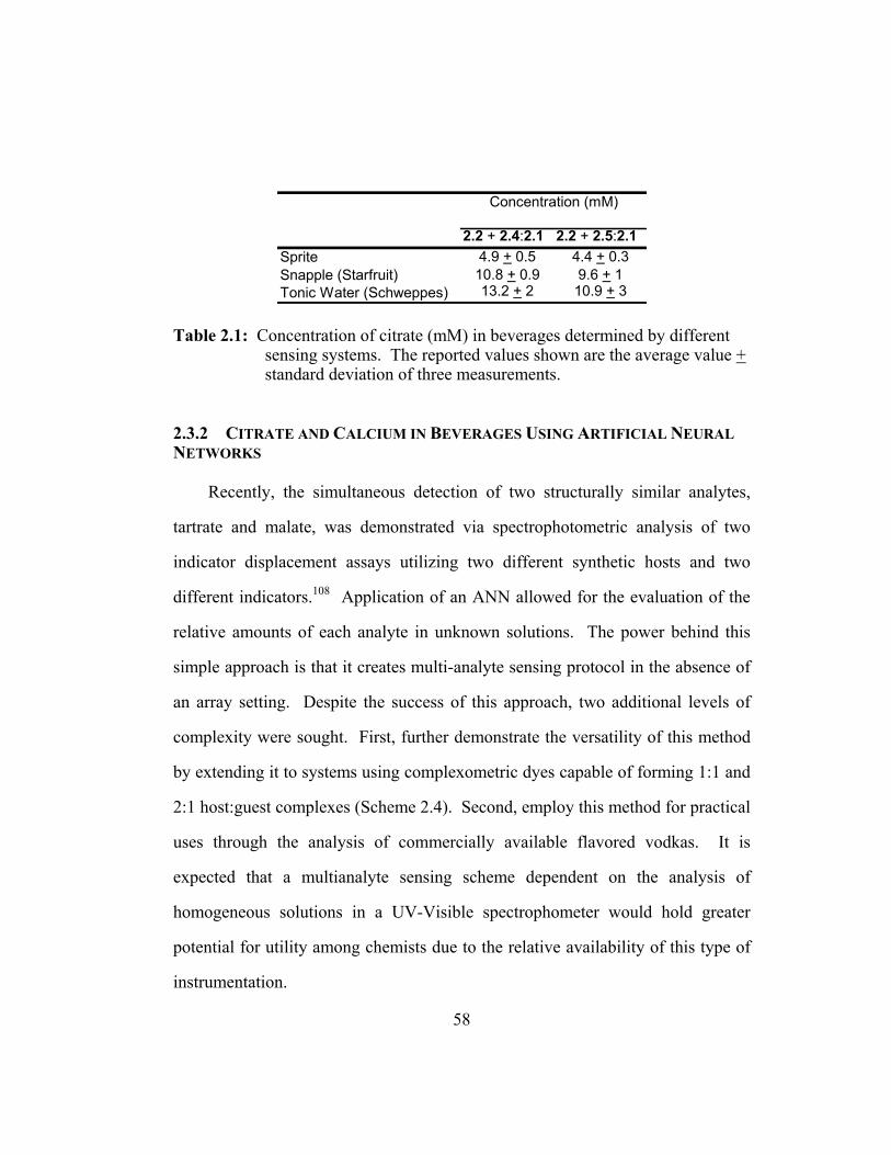
58

Table 2.1: Concentration of citrate (mM) in beverages determined by different sensing systems. The reported values shown are the average value + standard deviation of three measurements.

2.3.2 CITRATE AND CALCIUM IN BEVERAGES USING ARTIFICIAL NEURAL NETWORKS

Recently, the simultaneous detection of two structurally similar analytes,

tartrate and malate, was demonstrated via spectrophotometric analysis of two

indicator displacement assays utilizing two different synthetic hosts and two

different indicators.108 Application of an ANN allowed for the evaluation of the

relative amounts of each analyte in unknown solutions. The power behind this

simple approach is that it creates multi-analyte sensing protocol in the absence of

an array setting. Despite the success of this approach, two additional levels of

complexity were sought. First, further demonstrate the versatility of this method

by extending it to systems using complexometric dyes capable of forming 1:1 and

2:1 host:guest complexes (Scheme 2.4). Second, employ this method for practical

uses through the analysis of commercially available flavored vodkas. It is

expected that a multianalyte sensing scheme dependent on the analysis of

homogeneous solutions in a UV-Visible spectrophometer would hold greater

potential for utility among chemists due to the relative availability of this type of

instrumentation.

2.2 + 2.4:2.1 2.2 + 2.5:2.1Sprite 4.9 + 0.5 4.4 + 0.3Snapple (Starfruit) 10.8 + 0.9 9.6 + 1Tonic Water (Schweppes) 13.2 + 2 10.9 + 3

Concentration (mM)

59

The host (2.1) and indicator, xylenol orange (2.4), discussed earlier were

chosen for this study due to their established affinities for citrate (2.2) and

calcium (Ca(II)), respectively.109 The presence of the guanidinium groups on the

host 2.1 is known to impart affinity to carboxylates,91-95 while the iminiodiacetic

acid moieties on the indicator 2.4 have been shown to bind divalent cations like

calcium.103-106 Also, the xylenol orange indicator was chosen due to the

characteristic color change or λmax shift observed earlier in similar systems

resulting in a larger dynamic range with which to work.

The signaling mechanism envisioned is an indicator-displacement assay

which has often been exploited by the Anslyn group.91-95 The signaling scheme is

executed by adding a host molecule to an indicator adorned with binding groups

similar in charge or geometry as the target analyte. Once a H:I complex is

formed, the analyte of interest is introduced and the H:I equilibrium is disrupted.

As the analyte binds preferentially to the host, an optically measurable response

results due to the changes in the microenvironment of the indicator.

The training set (matrix) needed for the identification and quantification of

calcium and citrate was carried out by obtaining UV-Visible spectra of a two-

component sensing ensemble of 2.1 and 2.4 in solution. With this approach,

several absorbance measurements at different wavelengths from a solution

containing this sensing ensemble can serve as unique data inputs (or a fingerprint

response) allowing for identification and quantification of components present in

the solution. In this regard, the concentration of the host and indicator were

maintained at a constant concentration while separate UV-Visible spectra were

60

obtained for each addition of various amounts of calcium and citrate. Figure 2.8

is a general outline for the matrix of spectra envisioned for the training set.

Figure 2.8: The approach taken to obtain data via UV-Vis spectroscopy for the two-component sensing ensemble, where spectra were recorded at various concentrations (mM) of calcium and citrate.

Eighty discrete spectra resulted by systematically changing the

concentrations of calcium in 50 µM increments ranging between 0 and 400 µM

and also changing the concentrations of citrate in 100 µM increments ranging

between 0 and 800 µM. An example of the spectral difference between the

binding of varying ratios of calcium and citrate to 2.1 and 2.4 is illustrated in

Figure 2.9. These two spectra show that a unique response is detected when a

compleximetric dye is combined with a synthetic receptor upon exposure to

mixtures of two different analytes.

0

0 0.05

0.1

0.2

0.1

Calcium[mM]

Citr

ate

[mM

]… 0.4

0.8

…0

0 0.05

0.1

0.2

0.1

Calcium[mM]

Citr

ate

[mM

]… 0.4

0.8

…

61

Figure 2.9: Representative UV-Vis spectra of the indicator-displacement assays created when a solution containing 2.4 (240 µM) and 2.1 (10 µM) is titrated with various concentrations of calcium and 2.2 in 25% (v/v) vodka in water with 10 mM HEPES buffer at pH 7.5. [(▬)Calcium at 400 µM and citrate at 100 µM] and [(─ ─) Calcium at 50 µM and citrate at 600 µM] Inside tick marks on the x-axis illustrate the 25 wavelengths chosen to use in the ANN analysis.

As shown in Scheme 2.4, the equilibria of this system are complex.

Detection of these complexes would normally prove to be difficult because many

of the species that may exist in the solution do not contain chromophoric groups

for optical monitoring by UV-Visible or fluorescence spectroscopy. In fact, only

the presence of the complexometric dye allows for optical monitoring of the

events occurring in the solution. However, the spectrophotometric changes that

occur upon introduction of different analytes to the solution are subtle (Figure

2.9) and these subtle differences can be extracted quantitatively through the

application of pattern recognition.

Wavelength (nm)

Abso

rban

ce

0.20

0.35

0400 450 550 650

Wavelength (nm)

Abso

rban

ce

0.20

0.35

0400 450 550 650

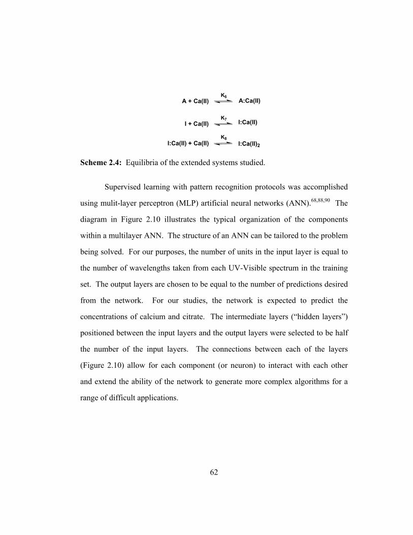
62

Scheme 2.4: Equilibria of the extended systems studied.

Supervised learning with pattern recognition protocols was accomplished

using mulit-layer perceptron (MLP) artificial neural networks (ANN).68,88,90 The

diagram in Figure 2.10 illustrates the typical organization of the components

within a multilayer ANN. The structure of an ANN can be tailored to the problem

being solved. For our purposes, the number of units in the input layer is equal to

the number of wavelengths taken from each UV-Visible spectrum in the training

set. The output layers are chosen to be equal to the number of predictions desired

from the network. For our studies, the network is expected to predict the

concentrations of calcium and citrate. The intermediate layers (“hidden layers”)

positioned between the input layers and the output layers were selected to be half

the number of the input layers. The connections between each of the layers

(Figure 2.10) allow for each component (or neuron) to interact with each other

and extend the ability of the network to generate more complex algorithms for a

range of difficult applications.

A + Ca(II) A:Ca(II)K6

I + Ca(II) I:Ca(II)K7

I:Ca(II) + Ca(II)K8

I:Ca(II)2

63

Figure 2.10: General representation of the multilayer ANN used for the analysis of flavored vodkas. The ANN is composed of an input layer, a variable number of hidden layers, and an output layer.

With the network trained, “unknowns” or inputs not present in the matrix can

be supplied into the trained network so that the previously formed algorithms can

attempt to calculate an output value. All but four of the spectra were used to train

the ANN using 25 wavelengths from each titration. The four traces that were

omitted from the training set were utilized as test points to evaluate the network’s

ability to extrapolate and therefore gage the performance of the ANN matrix. The

absolute error within the matrix for the output values of the test points ranged

from 2.2% to 17% (Table 2.2A).

[Calcium]

[Citrate]

Output Layer(concentrations)

Hidden Layers(processing nodes)

Input Layers(ABS @ each λ)

[Calcium]

[Citrate]

[Calcium]

[Citrate]

Output Layer(concentrations)

Hidden Layers(processing nodes)

Input Layers(ABS @ each λ)

64

Table 2.2: (A) Concentration of citrate (mM) and calcium (mM) in the validation test points samples determined by the two-component sensing system and ANN analysis. The reported values shown are the average value + standard deviation of three measurements with the percent different shown in parenthesis. (B) Concentration of citrate (mM) and calcium (mM) in various flavored Smirnoff ® vodkas determined by ANN and NMR analysis.

Despite the fact that the relative error associated with the output values for

each test point was less than 30%, independent verification of the individual

citrate concentrations of the unknowns reported for the flavored vodka samples

was carried out by other techniques. Given the good correlation between citrate

and Ca(II) found in Table 2.2, the focus here is on one component for verification:

citrate. The amount of citrate present in each flavored vodka sample was

accomplished by a NMR analysis. As shown in Table 2.2B, verification of citrate

concentrations by NMR gave values with a percent difference ranging from 1.7%

for the vanilla flavor to 33% for the green apple flavor. These values are in good

agreement, but it is believed that increasing the number of spectra obtained for the

training matrix would improve the accuracy and reduce the error of the

A

B

Vodka NMR AnalysisFlavor [Citrate (mM)] [Calcium (mM)] [Citrate (mM)]

Citrus Twist 0.98 0.72 0.90Orange 0.31 0.21 0.44Vanilla 1.18 0.74 1.16

Green Apple 1.55 0.02 1.04Raspberry 1.37 0.11 1.30

Predicted Values from ANN

[Citrate (mM)] [Calcium (mM)] [Citrate (mM)] [Calcium (mM)]0.00 0.10 0.03 +/- 0.01 (3.4%) 0.12 +/- 0.04 (14%)0.20 0.40 0.15 +/- 0.03 (27%) 0.37 +/- 0.01 (9.5%)0.40 0.15 0.347 +/- 0.005 (22.1%) 0.121 +/- 0.002 (30.1%)0.60 0.20 0.56 +/- 0.01 (7.7%) 0.179 +/- 0.001 (11.5%)0.80 0.35 0.769 +/- 0.0005 (4.41%) 0.037 +/- 0.009 (4.4%)

Real Values Predicted Values

65

methodology presented here. In addition, it was observed that the values reported

by both the ANN and the NMR methods indicate a trend of increasing citrate

concentrations in the vanilla, green apple, and raspberry flavored vodkas

compared to the orange and citrus twist flavors.

In conclusion, the combination of indicator-displacement assays and a

synthetic host with pattern recognition algorithms generates a useful sensing

strategy. Also, we successfully extended this method to encompass a practical

application such as the analysis of commercially flavored vodkas. This detection

method demonstrated that concentrations of more than one analyte can be

determined in a single analysis without the need for an array or sophisticated

instrumentation.

2.4 Summary

The competitive indicator method has been extended to systems

containing both 1:1 and 1:2 molecular complexes. Such competition assays give

a facile method of determining the concentration of a target analyte without

introducing additional covalent structure in the synthetic receptor. In general, we

predict that the use of complexometric dyes that have similar functionalities to

that of the analyte of interest can be used to generate many different colorimetric

competition assays.

In addition, the application of ANNs to a set of UV-Visible spectra

extends the utility of indicator-displacement assays to analyze two analytes with

one host and one indicator without the need for an array platform. In conclusion,

66

sophisticated hosts can be interfaced with different indicators to create simple but

powerful sensing systems for the analysis of analytes in aqueous media.

67

2.5 Experimental

2.5.1 MATERIALS

All the solvents used in spectrophotometric studies were of spectroscopic

grade and purchased from Aldrich. Xylenol orange and methylthymol blue were

obtained from Aldrich and used without further purification. The calcium nitrate

was obtained from Fisher Scientific and used without further purification. Buffer

components were of reagent grade. The synthesis of 2.1 has been previously

reported.92

2.5.2 ABSORPTION STUDIES

The absorption spectra were recorded on a Beckman DU-640 UV/Visible

spectrophotometer. All spectrophotometric measurements were done at a

constant pH (7.5) in 10 mM HEPES at room temperature (25oC). Solutions were

measured in a 1.00 cm (3 mL) quartz cuvette. The solvent system employed for

all the titration experiments was a 25 % (v/v) water in methanol mixture.

The first set of absorption titrations (adding 2.1 to 2.4 and 2.1 to 2.5) were

performed by keeping the concentration of the indicator constant (55 µM) while

varying the concentration of 2.1. Data obtained from these titrations were used in

the determination of affinity constants for 2.1 to 2.4 and 2.1 to 2.5. The second

set of absorption titrations (adding 2.2 to 2.1:2.4 and 2.2 to 2.1:2.5) were

performed by keeping both the concentration of each indicator 2.4 and 2.5 (55

µM) and 2.1 (1.13 mM) constant, while varying the concentration of 2.2. Data

68

obtained from these titrations were used to generate calibration curves for citrate

(Table 2.1).

The second set of absorption titrations (generation of the matrix for the

ANN) were performed by keeping the concentration of the H2:I solution constant

(0.24 mM 2.1 and 0.01 mM 2.4) and adding both Ca(NO3)2 and 2.2 in varying

concentrations to separate solutions of 2.1:2.5. All solutions were buffered at pH

7.5 with HEPES buffer (10 mM) in 75% Smirnoff Vodka in water (v/v). Nine

separate solutions were made that contained 0.5 mL of the H2I solution, 100 µL of

a 10 mM Ca(NO3)2, and aliquots of a 20 mM Citrate solution brought to a volume

of 1.00 mL with the solvent system described above. Next, nine other solutions

were prepared in the same manner without the addition of the Ca(NO3)2 solution.

For the “leave-one-out” strategy, four test solutions were prepared to evaluate the

network’s ability to extrapolate and are shown in Table 2.2.

2.4.3 EXTRACTION OF BINDING CONSTANTS

The binding constants of 2.1 to each indicator was determined from the

data obtained from the two titration experiments described earlier. The

absorbance was recorded at 577 nm for the addition of 2.1 to 2.4 assay and 607

nm for the addition of 2.1 to 2.5 assay. The binding constants were determined

form the plot of (∆A/b) vs. total citrate concentration using Eq. 2.17 where b =

1.00 cm, [Hi] was found using Eq. 2.20, [IT] is the total indicator concentration

(55 µM), ∆ε1 = εI:H-εI and ∆ε2 = εI:H2-εI. The values used for [Hi] were found by

solving Eq. 2.20 in Mathematica 3.0 for each [HT] known experimentally (0-1.4

mM) and initial estimates of K1, K2, ∆ε1, and ∆ε2. The values for ∆ε1 and ∆ε2 for

69

the 2.1 + 2.4 assay were found to be 2.41 x 104 cm-1 M-1 and 1.13 x 104 cm-1 M-1,

respectively. The values for ∆ε1 and ∆ε2 for the 2.1 + 2.5 assay were found to be

2.75 x 104 cm-1 M-1 and 8.19 x 103 cm-1 M-1, respectively.

2.5.4 EVALUATION OF BEVERAGES

For the UV-Vis citrate assay, sample preparation was dependent on the

beverage being analyzed. The tonic water and Sprite® samples were sonicated and

the pH of each sample was then adjusted to 7.5 with aqueous sodium hydroxide.

The Snapple® fruit drink was filtered. This solution was then brought to a pH of

7.5 with additions of aqueous sodium hydroxide. An aliquot (25.0 mL) of each

beverage sample was lyophilized to remove the water. The residue was then re-

dissolved in 25% (v/v) water in methanol (10.0 mL). An aliquot (300 µL) of this

beverage solution was added to the sensing ensemble (55 µM 2.4 or 2.5 and 1.13

mM 2.1) and brought to a total volume of 2.00 mL. Then subsequent portions of

this solution (10-200 µL) were added to the sensing ensemble (1.00 mL). An

absorbance value was recorded for each addition and the corresponding citrate

concentration value was obtained from the calibration curve (Figure 2.8). The

final values reported in Table 2.1 were obtained by multiplying the value

determined from the calibration curve by the dilution factor.

For the analysis of flavored vodkas, sample preparation proceeded by

taking an aliquot (25.0 mL) of each flavored vodka and evaporating any ethanol.

To each residue, 100 mL of deionized water was added and each sample was

lyophilized to remove the water. The residue was then dissolved in 25% (v/v)

water in vodka (5.0 mL). An aliquot (100 µL) of this beverage solution was

70

added to the sensing ensemble (0.2 mM 2.1 and 0.01 mM 2.4) and brought to a

total volume of 1.00 mL. An absorbance value was recorded three times for each

sample and the corresponding citrate concentration and calcium values were

obtained from the matrix (Table 2.2). The final values reported in Table 2.2 were

obtained by multiplying the value determined from the ANN by the dilution

factor.

2.5.6 NEURAL NETWORK PROCESSING

Processing of the UV-Vis measurements was accomplished using

Statistica Artificial Neural Network software (version 5.5) for the multi-layered

perceptron MLP analysis. No pre-processing of the data was attempted.

71

CHAPTER 3: DIFFERENTIAL RECEPTORS CREATE PATTERNS DIAGNOSTIC FOR NUCLEOTIDE

PHOSPHATES

3.0 Introduction

In recent years, approaches to chemical sensing have been shifting

towards the development of devices capable of simultaneous detection of multiple

analytes rather than single analyte sensors.75,78,79,110,111 In the previous chapter,

indicator-displacement assays were shown the ability to create mulitanalyte

sensing schemes without the use of an array platform. Another application for the

indicator-displacement assay is discussed here in the context of a multi-

component sensing array device.

In this regard, a resin-bound library of receptors is integrated into a

multicomponent sensing device. Optimization of the experimental conditions

necessary for successfully signaling the presence of various nucleotide phosphates

in solution using an indicator-displacement assay is discussed. Specifically, each

chemosensor is placed into a micromachined cavity within a silicon wafer, and

the optical changes observed by a charged-coupled device (CCD) result in near-

real-time digital analysis of solutions. Also, the application of principal

component analysis (PCA) to quantitatively compare the data sets from each

analysis is presented. In summary, a multi-faceted approach was used to develop

a combinatorial sensor system capable of sensing biologically relevant

phosphates.

72

3.1 Development of Combinatorial Receptors for Nucleotide Phosphates

The Anslyn, McDevitt, and Shear groups have exploited the use of resins

modified with known chemical indicators 81, enzymes85, and immunoglobulins84

to detect many analytes in complex fluids within the array platform. In one

approach, a combinatorial library of resin-bound receptors was developed in an

effort to combine the University of Texas sensor array technology with the power

of combinatorial chemistry97. Based on these studies, adenosine 5’-triphosphate

(ATP) was chosen as the target analyte for proof of principle and potential

applications in medical diagnostics and microbiology.

Scheme 3.1: General molecular structure of combinatorial resin-bound receptor library (3.1) and fluorescein (3.2) used to sense for nucleotide phosphates in the array platform.

The design of the anchored receptor (3.1) includes a 1,3,5-trisubstituted-

2,4,6-triethylbenzene scaffold coupled with peptide libraries (Scheme 3.1). The

scaffold was linked to the resin bead via a urea linkage to a lysine. The scaffold

O HN NH

O HN NH

NH2

NH

NH

O

R1

HNO

HN

R2 ONH3

R3

+H2N

NHH3N

+

NH

ONH

R1OHN

R2

H3N

R3

O+

+

+

PEG NH

Designed core

Tripeptidearm

ResinOO O

O

O

-

-

(Fluorescein)

3.1 3.2

O HN NH

O HN NH

NH2

NH

NH

O

R1

HNO

HN

R2 ONH3

R3

+H2N

NHH3N

+

NH

ONH

R1OHN

R2

H3N

R3

O+

+

+

PEG NH

Designed core

Tripeptidearm

ResinO HN N

H

O HN NH

NH2

NH

NH

O

R1

HNO

HN

R2 ONH3

R3

+H2N

NHH3N

+

NH

ONH

R1OHN

R2

H3N

R3

O+

+

+

PEG NH

Designed core

Tripeptidearm

ResinOO O

O

O

-

-

(Fluorescein)

OO O

O

O

-

-

(Fluorescein)

3.1 3.2

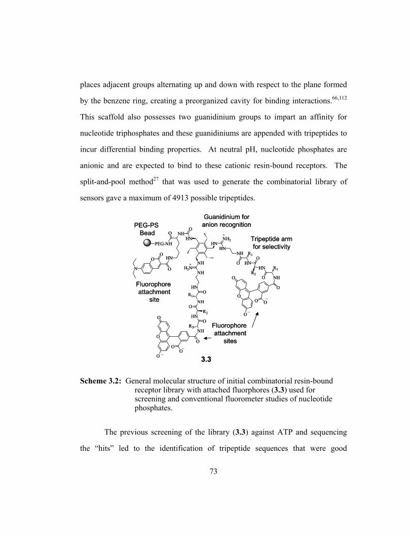
73

places adjacent groups alternating up and down with respect to the plane formed

by the benzene ring, creating a preorganized cavity for binding interactions.66,112

This scaffold also possesses two guanidinium groups to impart an affinity for

nucleotide triphosphates and these guanidiniums are appended with tripeptides to

incur differential binding properties. At neutral pH, nucleotide phosphates are

anionic and are expected to bind to these cationic resin-bound receptors. The

split-and-pool method27 that was used to generate the combinatorial library of

sensors gave a maximum of 4913 possible tripeptides.

Scheme 3.2: General molecular structure of initial combinatorial resin-bound receptor library with attached fluorphores (3.3) used for screening and conventional fluorometer studies of nucleotide phosphates.

The previous screening of the library (3.3) against ATP and sequencing

the “hits” led to the identification of tripeptide sequences that were good

PEG-NH

O NHO

HN

NH

HN

NH

NH2

HNNH

H2N

HN

HN

O

NHR1

O

HNR2

O

NHR3

O HN

R1O

R2

HN

O NH

R3

OO

O

OO

O

O

OO

N

O

O

O

O

OO

PEG-PS Bead

Guanidinium foranion recognition

Tripeptide armfor selectivity

Fluorophore attachment

sites


site

3.3

PEG-NH

O NHO

HN

NH

HN

NH

NH2

HNNH

H2N

HN

HN

O

NHR1

O

HNR2

O

NHR3

O HN

R1O

R2

HN

O NH

R3

OO

O

OO

O

O

OO

N

O

O

O

O

OO

PEG-PS Bead

Guanidinium foranion recognition

Tripeptide armfor selectivity


sites


site

3.3

74

candidates for binding the target analyte. Fluorescently labeled N-

methylanthraniloyl-ATP (MANT-ATP) was used to screen the combinatorial

library of receptors (3.3) for members that were selective for ATP.97

Approximately 15% of the library members were found to bind MANT-ATP to

varying degrees. Several of the highly fluorescent sensors (“hits”) and a few of

the nonfluorescent sensors (“misses”) were removed and sequenced. From the

sequencing results, three members that were fluorescent and one member that was

not fluorescent were arbitrarily chosen for resynthesis in bulk quantities. These

sensors (3.3) shown in Scheme 3.2 also included the addition of an attached 5-

carboxyfluorescein molecule at the end of the tripeptide arms to be used in further

fluorescent studies.

Fluorescent studies were done in a conventional fluorometer using a

“monolayer” of beads of one member (Ser-Tyr-Ser) in the 3.3 library to study the

stoichiometry and affinity constant of these sensors with various nucleotide

phosphates.97 The monolayer consists of a thin layer of beads sandwiched

between two layers of gold mesh on a glass slide. An increase in the emission of

fluorescein was observed upon binding of ATP (Figure 3.1). A binding constant

of 3.4*103 M-1 was calculated from these studies.97 A large spectral response was

observed upon addition of ATP compared to that of adenosine 5’-monophosphate

(AMP) and guanosine 5’-triphosphate (GTP) in a sulphonate (4-(2-

hydroxyethyl)piperazine ethanesulfonic acid-N-(2-hydroxyethyl)piperazine-N’-(2-

ethanesulfonic acid)) or HEPES buffer at pH 7.4. These results suggest that

selected members of the 3.3 library are responsive to nucleotide phosphates.

75

Figure 3.1: Isotherm plots of the Ser-Tyr-Ser library (3.3) member in 200 mM HEPES buffer solution at pH 7.4. Comparison of fluorescence response to additions of ATP, GTP, and AMP solutions shows 3.3 selectivity of ATP over the other phosphates.97

Earlier, it was postulated that this combinatorial library of receptors biased

toward a class of analytes would be effective in an array setting. To this end, a

library of chemosensors (3.1) was integrated into a chip-based array platform in

order to develop a more versatile strategy for characterizing nucleotide

phosphates in aqueous solutions.81,82 The objective of this dissertation work is to

determine whether the patterns generated by a library of receptors in an array can

discriminate between structurally similar compounds like ATP and GTP.

76

3.2 Array Platform Studies

3.2.1 SELECTION OF INDICATOR AND EXPERIMENTAL CONDITIONS

As mentioned earlier, the optical assay envisioned was an indicator-

displacement assay between the resin-bound receptor and an anionic dye

molecule. Fluorescein (3.2) was chosen because it has been proven successful in

earlier studies97 with a similar library of receptors (3.3), and it is commercially

available. It possesses a carboxylate and phenol on the xanthene ring that is

known to change color with protination state.113 Since this probe is a pH

indicator, all solutions were buffered with HEPES at pH 7.5. At this pH, it was

expected that the fluorescein would be present in its dianionic form and associate

in some fashion with the cationic resin-bound receptor resulting in a color change

to each resin bead. Introduction of ATP to the sensing ensemble would disrupt

this association and, upon formation of an ATP-receptor interaction, cause a

measurable color change (Figure 3.2). In other words, sensing of nucleotide

phosphates will be accomplished with indicator-displacement assays by optically

monitoring intensity changes in the signal of the dye molecule as the analyte

binds.

77

Figure 3.2: Signal transduction scheme used to detect nucleotide phosphates within the resin-bound sensor (3.1). AAn = amino acid.

To explore the feasibility of the dye displacement assay, a series of

experiments were completed using a variety of different experimental conditions.

All optical measurements are done colorimetrically using bright-field microscopy

in order to avoid difficulties associated with epi-fluorescence measurements.

Despite the fluorescent nature of fluorescein, the dye is used as a colorimetric

indicator in these studies. Local concentrations of dye in the bead interior leads to

high effective loading levels allowing for the completion of absorbance based

measurements.

3.2.2 ASSAY OPTIMIZATION

There are several important issues to consider in the development of a new

sensing protocol for a library of receptors (3.1) attached to solid supports. In

order to sense for nucleotide phosphates, the anchored receptors (3.1) should

undergo reversible and selective binding of the analyte. The optical changes that

result due to the association of 3.2 to the anchored receptor (3.1) are determined,

and the mechanisms associated with the binding of nucleotide phosphate and dye

78

to the receptor on the resin is also rationalized. Hence, a series of experiments are

outlined throughout this section in order to investigate these scientific questions.

Figure 3.3: (A) Scanning electron micrograph of representative 3 x 4 microarray containing glass beads.114 (B) Design of flow cell used in experiments.

Since the library of resin-bound receptors (3.1) had 4913 unique members,

each parameter investigated within the array used a 7 x 5 array platform to

maximize the number of candidates screened in each experiment. A scanning

electron micrograph of a representative 3 x 4 array platform is shown in Figure

3.3A. Sample delivery to the chemosensors occurs using a previously described

flow cell.81 A schematic of the flow cell is shown in Figure 3.3B. The sample is

introduced over the array and passes around and through the beads to exit the

bottom of the wells. Red, green, and blue (RGB) transmitted light intensity

values are recorded for each bead in the array over the period of the assay via a

CCD. “Effective absorbance” values for each color channel can then be

calculated according to Beer’s Law (Eq. 3.1).

oIIA log−= Eq. 3.1

500 µm

Array

A B

500 µm

Array

A B

500 µm500 µm500 µm

ArrayArray

A B

79

Included in each experiment within the array are five control beads that

consist of the same matrix as those used in the synthesis of 3.1 (TentaGel-NH2)

and were chemically derivatized with acetic anhyride (3.4) and 5-

carboxyfluorescein (3.5). With this arrangement, the acetylated resins (3.4)

function as blanks and the fluorescein-appended resins (3.5) allow for the pH of

the solutions passing through the flow cell to be monitored.

First, the binding properties of 3.2 to 3.1 were investigated. This was

accomplished by randomly choosing thirty beads from the series of receptors

(3.1), three blank beads (3.4), and two resin-bound fluorescein beads (3.5) and

placing them into the microarray (Figure 3.4A). A 0.03 mM solution of 3.2 was

introduced into the array with the eluting buffer (25 mM HEPES pH 7.5) at 1

mL/min. The CCD camera recorded the dye solution passing through the array

for 12 min. Since the λmax for fluorescein lies within the blue channel region,

“effective absorbance” values (AB) were calculated using Eq. 3.2 (See

Experimental).

oB

BB I

IA log−= Eq. 3.2

Figure 3.4B is a graphical representation of the images collected by the

CCD camera during this experiment. This plot demonstrates that the library of

receptors (3.1) associate with 3.2 to varying degrees. Blank beads (bead #1 in

Figure 3.4B) developed little or no orange color indicating that the dye did not

associate within the matrix of the bead through hydrophobic effects. Fluorescein

beads (3.5) remained unchanged throughout the assay indicating that the pH

remains constant (data not shown). It is also interesting to note that beads with

80

faster rates of dye uptake do not necessarily retain or associate with more

fluorescein (or have a higher AB value). These observations are consistent with

the presence of some amount of chemical diversity associated with each member

within the 3.1 library.

Figure 3.4: Differential dye (3.2) binding to the library of receptors (3.1, Beads 3, 4, 6, 7, 10 and 12). (A) Representative image of the chemosensors studied within the array after a solution of 3.2 was introduced. (B) Graphical representation of the data taken by the CCD camera upon an injection of 0.03 M solution of 3.2 to the array of beads with eluting 25 mM HEPES buffer at pH 7.5. (Bead #1 (3.4) took up little or no dye.)

Ultimately, it was envisioned to be able to compare the responses of one

resin-bound member of the library (3.1) to different nucleotide phosphates. In

order to obtain any relevant statistical information from these types of

experiments, a way of reproducibly returning each chemosensor to the same “zero

point” or baseline for repeated analysis needed to be determined. This was

BlankBeads

LibraryBeads

Blu

e C

hann

el A

BS

Time (sec)0 35 700200

0.2

0.6

1.2

Bead 1

Bead 7

Bead 10

Bead 12

Bead 4

Bead 6

Bead 3

134

67

1012

A BBlankBeads

LibraryBeads

Blu

e C

hann

el A

BS

Time (sec)0 35 700200

0.2

0.6

1.2

Bead 1

Bead 7

Bead 10

Bead 12

Bead 4

Bead 6

Bead 3

134

67

1012

A B

81

accomplished through the removal of the residual dye after data extraction for a

set time period (5 min) by flowing a 30 mM sodium hydroxide solution over the

array containing the dye-loaded beads at a flow rate of 1mL/min so that charge

pairing between the dye (or the analyte) and the receptor would be disrupted, thus

allowing these compounds to be removed from the bead. Next, a small amount

(2.0 mL at a flow rate of 1mL/min for 5 min) of 10 mM hydrochloric acid would

be introduced to the array of beads with eluting buffer in an attempt to return the

microenvironment close to the original value. Finally, the original flowing buffer

(pH = 7.5) was reintroduced into the flow cell.

At this point, studies on the reproducibility of indicator uptake were

performed. Although the relative concentration of receptors on each bead is

unknown,115 it is only required for the purposes of the displacement assay that the

same absorbance value result within each library bead upon introduction of 3.2

from trial to trial. On a molecular level, one can consider each library bead as a

single receptor with n binding sites. Hence, experiments were designed to test the

reproducibility of the 3.1:3.2 association by introducing various concentrations of

fluorescein in 25 mM HEPES (pH 7.5) to an array containing the resin-bound

library of receptors (3.1).

82

Figure 3.5: Absorbance values plotted over time for an array containing four members of 3.1 library in eluting 25 mM HEPES buffer at pH 7.5. (A) Addition (2.0 mL pulse) of 3.2 solution at 0.30 mM. (B) Addition (2.0 mL pulse) of 3.2 solution at 3.0 mM.

Two separate absorbance plots of a dye pulse introduced into an array of

library beads over time at two different concentrations are shown in Figure 3.5.

After testing several different concentrations of dye solutions, it was determined

that one pulse of dye at a concentration of 0.3 mM in 25 mM HEPES (pH 7.5) at

the flow rate of 1.0 mL/min gave the most reproducible regeneration of color

from trial to trial for each bead compared to itself. A second 2.0 mL pulse of the

dye at the same concentration was integrated into the assay protocol to insure

saturation of all the binding sites on the receptor. This establishes a stable signal

in the presence of eluting buffer in repeated trials and maximizes the dynamic

range with which to work. As shown in Figure 3.5B, a dye pulse at a

concentration of 3.0 mM into the array of library beads caused a significant

Blu

e C

hann

el A

BS

Elapsed Time (sec)

0 100 900400

0.2

0.7

1.0

BA

Blu

e C

hann

el A

BS

Elapsed Time (sec)

0 100 900400

0.2

0.7

1.0

Blu

e C

hann

el A

BS

Elapsed Time (sec)

0 100 900400

0.2

0.7

1.0

BA

83

increase in absorbance values. Unlike in previous dye uptake studies, there was

no noticeable amount of dye removed from the 3.1 library beads by the typical

wash sequence. This was reasoned to be the result of exceeding the solubility

limit of the sensing ensemble and generating a precipitate.

As emphasized above, one of the primary goals of this effort involves the

development of dye displacement assays for discrimination of structurally similar

phosphonate analytes using combinatorial-bead arrays. As such, each bead

constitutes a new and unknown sensing ensemble whose properties and

characteristics differ from neighboring microsensors. To develop practical sensor

systems, it is convenient to be able to refresh and re-use chip ensembles so that

the reproducibility and discrimination capacity of the array can be deciphered.

Further, the definition of the assay conditions that yield the best analytical

characteristics much be defined and optimized using a series of sequential trials

with the same population of beads.

Table 3.1 illustrates the reproducibility of signal from trial to trial in one

experiment for the dye uptake protocol devised for ten 3.1 chemosensors in a

microarray. The number reported for each bead is the average of thirty

absorbance values calculated from images taken 5 sec apart by the CCD camera

of the microarray with eluting buffer at 1mL/min after injection of the two dye

pulses under ideal conditions. The variability in the absorbance values for dye

uptake ranged from 0.4-6.0% standard deviation over six trials.

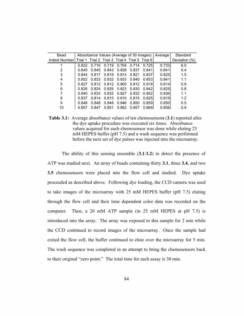
84

Table 3.1: Average absorbance values of ten chemosensors (3.1) reported after the dye uptake procedure was executed six times. Absorbance values acquired for each chemosensor was done while eluting 25 mM HEPES buffer (pH 7.5) and a wash sequence was performed before the next set of dye pulses was injected into the microarray.

The ability of this sensing ensemble (3.1:3.2) to detect the presence of

ATP was studied next. An array of beads containing thirty 3.1, three 3.4, and two

3.5 chemosensors were placed into the flow cell and studied. Dye uptake

proceeded as described above. Following dye loading, the CCD camera was used

to take images of the microarray with 25 mM HEPES buffer (pH 7.5) eluting

through the flow cell and their time dependent color data was recorded on the

computer. Then, a 20 mM ATP sample (in 25 mM HEPES at pH 7.5) is

introduced into the array. The array was exposed to this sample for 2 min while

the CCD continued to record images of the microarray. Once the sample had

exited the flow cell, the buffer continued to elute over the microarray for 5 min.

The wash sequence was completed in an attempt to bring the chemosensors back

to their original “zero point.” The total time for each assay is 30 min.

Bead Average Standard Indext Number Trial 1 Trial 2 Trial 3 Trial 4 Trial 5 Trial 6 Deviation (%)

1 0.822 0.716 0.719 0.704 0.714 0.725 0.733 6.02 0.845 0.845 0.843 0.839 0.837 0.841 0.841 0.43 0.844 0.817 0.819 0.814 0.821 0.837 0.825 1.54 0.852 0.833 0.832 0.833 0.840 0.853 0.841 1.15 0.827 0.812 0.812 0.805 0.812 0.818 0.814 0.96 0.826 0.824 0.826 0.823 0.830 0.842 0.829 0.87 0.840 0.833 0.832 0.827 0.832 0.852 0.836 1.18 0.837 0.814 0.815 0.810 0.815 0.825 0.819 1.29 0.848 0.848 0.848 0.846 0.850 0.859 0.850 0.510 0.857 0.847 0.851 0.852 0.857 0.869 0.856 0.9

Absorbance Values (Average of 30 images)

85

The assay was repeated three times, and the data extraction and RGB

analysis of these trials yields the following plot (Figure 3.6). The absorbance

traces seen in Figure 3.6 show that each sensing ensemble (3.1:3.2) maintains

color in the presence of flowing buffer. However, upon injection of ATP, the

absorbance values increase initially and then fall off at different rates. This initial

increase in color was attributed to a microenvironmental pH change to the

fluorescein from the formed association between 3.1 and ATP and subsequent

expulsion of the dye molecule from the binding pocket of 3.1. The disappearance

of color from each bead thereafter is rationalized to be the result of the dye

molecule, now free from the binding pocket, being washed out of the flow cell by

the eluting buffer. Notably, the off rates, or absorbance trace slopes observed

from Figure 3.6, for 3.2 from each library bead are reproducibly different. The

variability of signal for each individual bead compared to itself from trial-to-trial

is less than 5%. The response of the control beads was the same as seen in

previous experiments described earlier. Displacement rates, however, quantified

by slope measurements vary from bead to bead within an individual trial ranged

from by 7.0 – 86.0%.

86

Figure 3.6: Absorbance values plotted over time elapsed (7 min) for 3.1:3.2 in eluting 25 mM HEPES buffer at pH 7.5 upon successive cycles of dye uptake, 20 mM ATP solution injections, and the wash sequence.

To summarize the conditions used for the dye displacement assays, dye

uptake proceeds with a 2.0 mL injection of a 3.0 x 10-4 M fluorescein dye in a 25

mM HEPES solution at pH 7.5 via the fluid delivery system. A second 2.0 mL

injection of the dye solution is introduced to the array in order to more completely

load the library bead receptor sites with fluorescein. A buffered solution is

allowed then to pass through the flow cell for 5 min in order to achieve a stable

initial starting point for the assay. At this time, RGB absorbance data is obtained

for each bead in the array. The CCD camera continues to record data as the

nucleotide phosphate sample is injected into the array. Data extraction and

processing (See Experimental) allows for calculation of the dye displacement

rates of each bead after analyte injection. The residual dye within the library

beads is rinsed out through a series of basic and acidic solution washes. These

Elapsed Time (min)

Blu

e C

hann

el A

BS

0.2

1.0

1.8Trial 1 Trial 2 Trial 3

7 min0

Elapsed Time (min)

Blu

e C

hann

el A

BS

0.2

1.0

1.8Trial 1 Trial 2 Trial 3

7 min0

87

assay conditions allowed for a reproducible method for optically monitoring the

uptake and displacement of fluorescein from a combinatorial library of resin-

bound receptors towards the detection of various nucleotide phosphonates in

solution.

3.3 Nucleotide Phosphate Detection

3.3.1 BINDING DATA

As mentioned earlier, the purpose of our work is to determine whether the

combined signals from a library of receptors in an array can create a fingerprint

response that allows for discrimination of structurally similar compounds like

ATP, GTP, and AMP. In Section 3.2, many experimental conditions were

elucidated and tested in order to develop an assay that would reproducibly

generate a 3.1:3.2 sensing ensemble that signals the presence of a nucleotide

phosphate within the array platform. As seen in Scheme 3.3, the three samples to

be studied only vary slightly in structure (i.e. ATP vs. GTP only varies in the

type of nucleotide base, and ATP vs. AMP varies by the number of phosphate

esters). Here, experiments are described so that the optical responses from the

library of receptors upon introduction of these three different samples could be

monitored and evaluated.

88

Scheme 3.3: Molecular structures of the various nucleotide phosphates studied.

In one experiment, thirty beads from the library were randomly chosen,

given an index number, and placed in a micromachined chip-based array

platform. The RGB intensity values for the thirty library beads in the array were

recorded over time after a 2.0 mL injection of a 20 mM sample of ATP, GTP, or

AMP in 25 mM HEPES buffer (pH 7.5). Three trials were performed for each

sample for a total of nine trials, and absorbance values were calculated by taking

the negative log of the ratio of the blue channel intensity over the red channel

intensity for each bead.81,82 Figure 3.7A shows representative normalized

absorbance traces for two of the beads in the array after an injection of GTP.

Figure 3.7B shows a trace of the same two beads after an injection of AMP. The

range of relative standard deviation for regeneration of signal for each bead trial

to trial in this experiment was 1.2 - 2.6%.

N

HO O H

H HO

NN

N

NH2

OPH O

O

O -

adenosine 5’-monophosphate(AMP)

HN

HO OH

H HO

N

H N

N

OPOPOPO

O O O

O O O- - -

H2N

O

guanosine 5’-triphosphate(GTP)

NO

N2

HO OH

H H

NN

NH

OPOPOPH O

O O O

O O O- - -

adenosine 5’-triphosphate(ATP)

N

HO O H

H HO

NN

N

NH2

OPH O

O

O -

N

HO O H

H HO

NN

N

NH2

OPH O

O

O -

adenosine 5’-monophosphate(AMP)

HN

HO OH

H HO

N

H N

N

OPOPOPO

O O O

O O O- - -

H2N

O

HN

HO OH

H HO

N

H N

N

OPOPOPO

O O O

O O O- - -

H2N

O

guanosine 5’-triphosphate(GTP)

NO

N2

HO OH

H H

NN

NH

OPOPOPH O

O O O

O O O- - -

NO

N2

HO OH

H H

NN

NH

OPOPOPH O

O O O

O O O- - -

adenosine 5’-triphosphate(ATP)

89

Figure 3.7: Absorbance values plotted over time for 3.1:3.2 in eluting 25 mM HEPES buffer at pH 7.5. (A) Addition (2.0 mL pulse) of 20 mM GTP solution in 25 mM HEPES (pH 7.5). (B) Addition (2.0 mL pulse) of 20 mM AMP solution in 25 mM HEPES (pH 7.5). To aid in slope comparison, the plots were shifted so that the average of the initial 30 points prior to sample injection (not shown) had an absorbance of 1.00.

In Figure 3.7, A and B show representative normalized absorbance traces

for two of the beads in the array after an injection of GTP and AMP, respectively.

The slope of the absorbance values from 210-435 seconds was calculated for each

bead in each sample, and these values were used in the analysis because the

indicator-displacement rates were found to be most reproducible in this region for

comparison. Only two of the thirty beads are displayed in Figure 3.7 and the plots

were shifted so that the average of the initial 30 points prior to sample injection

(not shown) had an absorbance of 1.00 to help aid in slope comparison. The slope

of bead 28 differs by 40% between the AMP and GTP trials. Whereas, the slope

value for bead 23 in each plot differs by only 26%. Although these slopes are

easily differentiated by qualitative visual inspection, the rates of displacement for

Elapsed Time (sec)0 400250

Bead 28Bead 23

Elapsed Time (sec)

Nor

mal

ized

Abs

orba

nce

0 400250

9.0

1.04

1.0

Bead 28Bead 23

BA

Elapsed Time (sec)0 4002500 400250

Bead 28Bead 23Bead 28Bead 23

Elapsed Time (sec)

Nor

mal

ized

Abs

orba

nce

0 4002500 400250

9.0

1.04

1.0

Bead 28Bead 23Bead 28Bead 23

BA

90

several trials can be compared more quantitatively using pattern recognition

algorithms as described below.

3.3.2 APPLICATION OF PRINCIPAL COMPONENT ANALYSIS

The method of principle component analysis (PCA) was utilized to reduce

the dimensionality of the data set. For each of the nine trials, a slope value was

recorded for each of the thirty beads. To identify patterns in the data, a principal

component (PC) axis is calculated to lie along the line of maximum variance in

the original data. Subsequent PC axes lie along lines describing diminishing

levels of variance. The coordinates of the sample relative to the PC axes are

termed scores and can be used as an indicator of correlation between analytes.

Proximity in space on a score plot directly correlates to similarities in indicator

displacement rates. Figure 3.8 shows a two dimensional score plot for the first

two principal components (PC1 and PC2) with clustering of the AMP, GTP and

ATP samples with one possible ATP outlier. PCA demonstrates that the array of

library sensors can differentiate between structurally similar molecules such as

AMP, GTP and ATP.

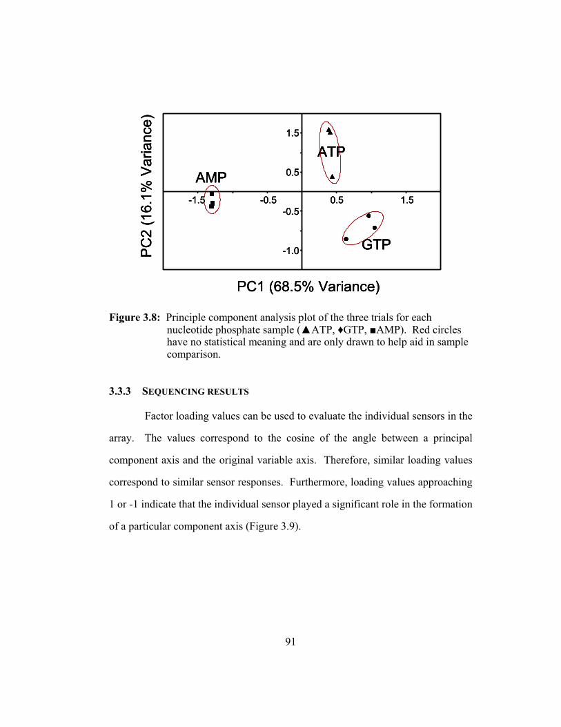
91

Figure 3.8: Principle component analysis plot of the three trials for each nucleotide phosphate sample (▲ATP, ♦GTP, ■AMP). Red circles have no statistical meaning and are only drawn to help aid in sample comparison.

3.3.3 SEQUENCING RESULTS

Factor loading values can be used to evaluate the individual sensors in the

array. The values correspond to the cosine of the angle between a principal

component axis and the original variable axis. Therefore, similar loading values

correspond to similar sensor responses. Furthermore, loading values approaching

1 or -1 indicate that the individual sensor played a significant role in the formation

of a particular component axis (Figure 3.9).

ATP

GTP

AMP

PC1 (68.5% Variance)

PC

2 (1

6.1%

Var

ianc

e)1.5

0.5

-0.5

-1.0

0.5 1.5-1.5 -0.5

ATP

GTP

AMP


PC

2 (1

6.1%

Var

ianc

e)1.5

0.5

-0.5

-1.0

0.5 1.5-1.5 -0.5

ATP

GTP

AMP

ATP

GTP

AMP


PC

2 (1

6.1%

Var

ianc

e)1.5

0.5

-0.5

-1.0

0.5 1.5-1.5 -0.5

92

Figure 3.9: Factor Loading Plot of the nine library (3.1) beads chosen for microsequencing.

Only nine beads were analyzed due to the high cost of peptide

microsequencing. Eight beads were chosen to be sequenced on the basis of their

large and nearly overlapping factor loading values (Figure 3.9 and Table 3.2).

Bead 14, which possessed the lowest values for each PC axis, was sequenced to

elucidate which receptors elicit minimal discrimination. It is interesting to note

that beads with high loading values possess serine (or the structurally similar

amino acid threonine) and other aromatic amino acids, as found in our earlier

screening of this library.97 Since 86% of the beads in the array had a factor

loading value with an absolute magnitude greater than 0.7 on PC1, it is thought

that the combination of these differential receptors is necessary for analyte

discrimination.

-1.2-1.0

-0.8 -0.4 0.0 0.4 0.8 1.2

-0.7

-0.4

-0.1

0.0

0.2

0.6

Bead 14

Bead 34

Bead 2

Bead 6Bead 25

Bead 24

Bead 23

Bead 28

Bead 33

Factor Loading (PC1)

Fact

or L

oadi

ng (P

C2)

-1.2-1.0

-0.8 -0.4 0.0 0.4 0.8 1.2

-0.7

-0.4

-0.1

0.0

0.2

0.6

Bead 14

Bead 34

Bead 2

Bead 6Bead 25

Bead 24

Bead 23

Bead 28

Bead 33

Factor Loading (PC1)

Fact

or L

oadi

ng (P

C2)

93

Table 3.2: Sequencing results and Factor Loading Values for the first two principal components (PC1 and PC2).

Even though statistical analysis of the sequencing results cannot be

performed due to the small number of beads analyzed, some conclusions can be

drawn for discussion nontheless. In Table 3.3, the amino acids found on each

bead and the distribution by position is catalogued. Of the seventeen amino acids

used in the synthesis of this library (3.1), several amino acids did not appear in

sequenced beads: glutamic acid, glutamine, and leucine. The most commonly

occurring amino acid was threonine and the two other amino acids (serine and

valine).

Table 3.3. Amino acid distribution by position.

Tripeptide Sequence Factor Loading Factor Loading Bead (PC1) (PC2) Index Number

Asp-Asn-Ser -0.98 0.14 28Phe-Trp-Phe -0.88 -0.16 23Thr-Thr-Ser -0.88 0.39 33Val-Asn-Tyr -0.84 -0.20 24Val-Pro-Ala 0.01 0.21 14Ala-Met-Thr 0.17 -0.91 34Val-Gly-Ile 0.74 -0.46 6Ser-His-Tyr 0.75 -0.47 25Thr-Thr-Ile 0.89 -0.36 2

His Asp Glu Ser Thr Asn Gln Ala Val Ile Leu Met Phe Tyr Trp Gly ProLocated on C' 1 1 2 1 3 1

Located in Middle 1 2 2 1 1 1 1Located on N' 2 1 1 2 1 2Total Residues 1 1 0 3 5 2 0 2 3 2 0 1 2 2 1 1 1

Amino AcidSpecialHydrophobicHydrophilic

94

3.4 Summary

A colorimetric displacement assay was performed and time dependent

imaging studies of the selected sensing ensembles result in differential responses

upon addition of ATP, AMP, or GTP. An advantage to this approach is that it

creates an array of sensors that gives a fingerprint response for each analyte.

Principal component analysis indicates that the library of chemosensors can

differentiate between ATP, GTP and AMP. Based upon factor loading values,

individual sensors from the library were sequenced to elucidate their chemical

composition.

In conclusion, the use of a combinatorial library of sensors and indicator-

displacement assays in the context of a chip-based array allows for the

differentiation of structurally similar analytes in aqueous solutions. The coupling

of supramolecular chemistry principles with pattern recognition lead to this new

protocol for sensing.

95

3.5 Experimental

3.5.1 MATERIALS

Triethylamine (Et3N) and dichloromethane (DCM) were refluxed over

calcium hydride and distilled when noted. Methanol was obtained from Fisher

Scientific. Sure seal anhydrous dimethylformamide (DMF), ATP, acetic

anhydride, GTP, AMP, diisopropylethylamine (DIEA), dicyclohexylcarbodiimide

(DCC), and fluorescein were obtained from Aldrich and used without further

purification. The compound 5(6)-carboxyfluorescein was obtained from

Molecular Probes, Inc. (Eugene, OR). The TentaGel amine (TentaGel-NH2)

resins (loading of 0.29 mmol/g), and 1-hydroxybenzotriazole (HOBt) were

obtained from NovaBiochem. The buffer 4-(2-hydroxyethyl)piperazine

ethanesulfonic acid-N-(2-hydroxyethyl)piperazine-N’-(2-ethanesulfonic acid)

(HEPES) was of reagent grade and all buffered solutions were brought to pH 7.5

by adjusting with the addition of sodium hydroxide (NaOH). The synthesis of 3.1

has been previously reported.81,97

3.5.2 SYNTHESIS OF CONTROL CHEMOSENSORS

Formation of the Acetylated TentaGel-NH2 resin (3.4). The preparation of

compound 3.4 went as follows: 3.0 mL (32 mmol) of acetic anhydride and 57 µL

(0.6 mmol) of Et3N were added to 200 mg of pre-washed TentaGel-NH2 resin

(0.29 mmol/g) to react for 1 hr. The acetylated resins were rinsed. The first

solution used in these series of rinses was DMF and the last was MeOH. The

96

ninhydrin test was negative. The resin were dried in vacuo for 4 hr and stored at

4oC.

Formation of the TentaGel-NH2 resin bound 5(6)-carboxyfluorescein

(3.5). Under argon, 5 mL of anhydrous DMF, 0.05 mg (1.4x10-4 mmol) of 5(6)-

carboxyfluorescein, 0.29 mg (1.4x10-3 mmol) DCC, and 0.19 mg (1.4x10-3 mmol)

HOBt were combined and allowed to stir for 30 min. In a separate reaction

vessel, 200.0 mg (0.06 mmol amine) of TentaGel-NH2 resin was rinsed with the

following solutions for 1 min: DMF, MeOH, 10% DIEA in DCM, DCM (twice),

MeOH, and DMF. The coupling agent and 0.25 µL (1.4x10-3 mmol) of DIEA

were added to the pre-rinsed resin and allowed to react for 1 hr. The resin were

rinsed three times with DMF and three times with MeOH (or until the color in

each wash disappeared) and dried in vacuo for 4 hr and stored at 4oC.

3.5.3 INSTRUMENTATION

The components of the micromachined array analysis system have been

previously described.81 In short, individually addressable microbeads were placed

into chemically etched cavities on a silicon wafer chip. The chip loaded with

microbeads was placed into a flow cell. The flow cell was positioned on an

Olympus SZX12 stereomicroscope stage that allowed for bottom illumination

(transmission) of the microbeads within the array to be observed through the

microscope optics. Solutions were introduced into the flow cell using an

Amersham Pharmacia Biotech ÄKTA Fast Protein Liquid Chromatograph

(FPLC) controlled by Unicorn 3.0 Software. The design of the flow cell allowed

for fluids to be introduced to the top of the array and forced down through each

97

bead-containing well and out through the drain. Optical changes occurring within

each bead in the array were observed through the microscope optics and captured

for analysis using a charge-coupled device (CCD) in conjunction with Image Pro

Plus 4.0 software (Media Cybernetics).

3.5.4 ASSAY CONDITIONS

Each assay was performed at room temperature under continuous flow

conditions. Indicator uptake proceeded with two cycles of 2.0 mL injections of a

0.30 mM fluorescein dye in a 25 mM HEPES buffer solution at pH 7.5 via the

fluid delivery system. To remove excess dye within the beads, the buffered

solution was allowed to pass through the flow cell at 1 mL/min for 5 min. At this

time, the CCD camera captured an image sequence file and the data was recorded

for later analysis. Next, a 2.0 mL nucleotide phosphate sample (20 mM) in a 25

mM HEPES buffer solution at pH 7.5 was injected into the array, and the CCD

camera recorded the disappearance of the indicator by the analyte. Finally, the

residual indicator within the library beads was rinsed out through a series of basic

(30 mM NaOH) and acidic (10 mM HCl) solution washes. The typical standard

deviation for regeneration of signal for each bead trial-to-trial ranged in these

experiments from 0.2 – 7.0%.

3.5.5 DATA COLLECTION AND PROCESSING.

Images of the array captured by the CCD camera were analyzed by

drawing areas of interest (AOI) in the central region of each bead and evaluating

their average red, green, and blue (RGB) intensities. Prior to the measurements,

the CCD imaging protocol was adjusted using a standard white balance

98

procedure. The library beads in the colorimetric assay developed an orange

coloration that was quantified by measuring the average blue pixel intensity

yielded by the CCD. This intensity, IB, was converted to the effective blue

absorbance, AB, using Beer’s Law (AB = - log (IB/IR)), where IR was the average

red pixel intensity for each bead in each image captured by the CCD camera.

Statistica Factor Analysis software (version 5.5) was utilized for the principal

component analysis (PCA). Blank beads (i.e. acylated Tentagel resins)

demonstrated that the indicator did not absorb hydrophobically into the bead

matrix.

3.5.6 PEPTIDE SEQUENCING

Beads were submitted to the Protein Microanalysis Facility at the

University of Texas at Austin for sequencing. A single bead is placed sandwiched

between a Zytex membrane and a glass fiber support and inserted into an Applied

Biosystems 477A pulsed liquid protein sequencer. The beads are washed with

ethyl acetate, dried, and then five cycles of Edman degradation methods are

performed.

99

CHAPTER 4: DETECTION OF NERVE AGENT DEGRADATION PRODUCTS IN WATER BY A COMBINATORIAL ARRAY SENSOR SYSTEM

4.0 Introduction

As described previously, a multi-faceted approach was taken in order to

develop a new signaling protocol that coupled a combinatorial library of receptors

with a multi-component sensing device. These methods demonstrated proof of

concept by using principal component analysis (PCA) to illustrate that a library of

chemosensors (3.1) can differentiate between adenosine 5’-triphosphate (ATP)

and guanosine 5’-triphosphate (GTP) in aqueous solutions. Herein, the

capabilities of this combinatorial array sensor system are expanded to characterize

other compounds such as hydrolysis products of nerve agents in order to illustrate

the general utility of this novel sensing scheme and demonstrate the suitability for

potential applications in verification analysis of chemical warfare agents (CWAs).

Of the different types of CWAs, the most lethal are the nerve agents which

act on the nervous system by reacting irreversibly with the enzyme

acetylcholinesterase.116 Typically CWAs such as Soman and VX hydrolyze

quickly under base; once they have been exposed to water, they decompose to

form non-volatile alkyl phosphonic acids (Scheme 4.1). These degradation

products are often used as an indirect way of monitoring the presence of

CWAs.117 However, detection of these compounds has proven to be difficult

100

because they do not contain chromophoric groups for optical monitoring by UV-

Visible or fluorescence spectroscopy.

Scheme 4.1: Common hydrolysis pathways for some nerve agents in water.

The development of a chip-based multianalyte detection system for

different nerve agent degradation products in solution is presented here. First, the

synthesis of a new combinatorial library of receptors is described and the studies

of these new chemosensors in the array platform are reported in order to help

further understand the role of the first series of combinatorial receptors described

earlier. A discussion contrasting the chemical diversity of the two different

combinatorial receptor libraries will be presented next. Third, studies that lend to

an understanding of the sensing protocol mechanism are discussed in the context

of redesigning and optimizing the assay conditions toward the successful

detection of various phosphonates in solution. Then a more scrutinous approach

of analyzing the raw data is taken by applying a series of “filters” or data input

Soman

VX

OP

O

F

H3C

OP

O

S

H3C

N

Pinacoylmethylphosphonic

acid (PMPA)

Ethylmethylphosphonic

acid (EMPA)

H3C P

O

O

O

H3C P

O

O

O

Methylphosphonicacid (MPA)

H3C P

O

OH

O

Soman

VX

OP

O

F

H3C

OP

O

S

H3C

N


acid (PMPA)


acid (EMPA)

H3C P

O

O

O

H3C P

O

O

O


H3C P

O

OH

O

Soman

VX

OP

O

F

H3C

OP

O

S

H3C

N

Soman

VX

OP

O

F

H3C

OP

O

S

H3C

N


acid (PMPA)


acid (EMPA)

H3C P

O

O

O

H3C P

O

O

O


acid (PMPA)


acid (EMPA)

H3C P

O

O

O

H3C P

O

O

O


H3C P

O

OH

O


H3C P

O

OH

O

101

strategies to the raw data and observing how these filters affect the outcome in the

PCA. To summarize, the improvements made to the combinatorial array sensing

protocol and the data input strategies are implemented to detect nerve agent

degradation products in solution within the array platform and used to

demonstrate that this sensing scheme is robust.

4.1 Evaluating Chemosensor Microenvironments

4.1.1 DESIGN AND SYNTHESIS OF “CONTROL” RESIN-BOUND LIBRARY

Following the successful development and demonstration of a library

populated microbead array approach for discrimination of biologically cofactors

(Chapter 3), the importance of the scaffolding present in the library of receptors

3.1 in producing such displacement assays was studied. Likewise, the necessity

of the rationally designed scaffold in the receptors used in those studies for

binding guests also needed to be investigated in order to achieve a more complete

understanding of the details of the indicator-displacement assays. To this end, a

new resin-bound combinatorial library solely composed of tripeptide chains was

synthesized (4.1) to serve as a control within chip-based CWA detection system.

102

Figure 4.1: (A) Schematic summarizing the split and pool method used to generate each library of resin-bound receptors. (B) General molecular structure of receptor library series 3.1. (C) General molecular structure of “control” resin-bound peptide library 4.1.

For the preparation of 4.1, the spit-and-pool method27 used previously was

employed (Figure 4.1A). It is an established method used to generate one-bead,

one-compound combinatorial libraries that allows for incorporation of standard

solid phase peptide 9-fluorenylmethoxycarbonyl chloroformate (Fmoc)

chemistry.118 With this popular method, oligomeric libraries are quickly

generated by coupling aliquots of resin in separate reaction vessels with a single

compound, recombining the resin and then dividing the resins again into aliquots

for another reaction to another single compound (Figure 4.1A).

The same TentaGel-NH2 resins used in the preparation of the 3.1 library of

receptors (Figure 4.1B) were chosen for the synthesis of the 4.1 library. These

O HN NH

O HN NH

NH

NH

NH

O

R1

HNO

HN

R2 ONH3

R3

HNNH

H3N

NH

ONH

R1OHN

R2

H3N

R3

O

Resin

Guanidinium

Tripeptide arm

PEG NH

C

A B

combinecombine

combinecombine

dividedivide

1

2

3.1

4.1

PEG-NH

O HN

R1O

NH

R2O NH2

R3

Tripeptide Arm

Resin

O HN NH

O HN NH

NH

NH

NH

O

R1

HNO

HN

R2 ONH3

R3

HNNH

H3N

NH

ONH

R1OHN

R2

H3N

R3

O

Resin

Guanidinium

Tripeptide arm

PEG NH

C

A B

combinecombine

combinecombine

dividedivide

combinecombine

combinecombine

dividedivide

1

2

3.1

4.1

PEG-NH

O HN

R1O

NH

R2O NH2

R3

Tripeptide Arm

Resin

103

resin-bound receptors contained tripeptides consisting of 19 amino acids (cysteine

was omitted to avoid the formation of intramolecular disulfide bonds). Solid

phase synthesis techniques were used to build each trimer on TentaGel-NH2

resins. A general scheme for the coupling of the amino acids to solid supports is

depicted in Figure 4.2.

Figure 4.2: General synthetic scheme for solid phase synthesis of trimers on TentaGel-NH2 resins.

The synthesis of each tripeptide on the resin began with the reaction of a

coupling agent (benzotriazole-1-yl-oxy-tris-pyrrolidino-phophonium

hexafluorophosphate, PyBOP) with an amino acid unit to form the activated ester.

The α amino group is protected as its Fmoc and the ε amino group protected with

an acid labile group (See Experimental). This ester was then reacted with a resin

bound amine in the presence of 4-methylmorpholine (NMM) to form an amide

linkage to the solid support. At this point a Kaiser test119 would be performed.

All tests were negative (no free amines present) indicating that each coupling had

gone to completion. The α-protecting group, Fmoc, was then removed from the

anchored amino acid with dilute base (20% piperidine in dimethylformamide).

The resins would be recombined, washed, and separated into different reaction

vessels where an additional amino acid monomer unit would be added in the same

R

O

OHR

OPyBOP

OR’

NH2

NO

RHNMM

Amino acid Activated ester Resin boundamino acid

R

O

OHR

OPyBOP

OR’

NH2

NO

RHNMMR

O

OHR

OPyBOP

OR’

NH2NH2

NNO

RHNMM

Amino acid Activated ester Resin boundamino acid

104

manner as described above. This process of splitting, coupling, deprotection, and

pooling of the resins was repeated twice more. The ε−Boc protecting groups were

ultimately removed from the resin-bound trimers under acidic conditions (50%

trifluoroacetic acid in dichloromethane). A combinatorial library of 6859

members (the theoretical maximum) was prepared and the general structure of

library 4.1 is shown in Figure 4.1C.

4.1.2 ARRAY PLATFORM STUDIES

In order to gain a further understanding of how the presence of the

receptors on the bead modify the microenvironment of the resin matrix and their

effects on the displacement assays, studies were performed utilizing both series of

receptor libraries within the array platform. The main components of this array

platform are chemically derivatized beads, a silicon microchip, a flow cell, and a

charged-coupled device (CCD) camera, all having been described earlier.81,82

Studies of the newly synthesized resin-bound receptor library (4.1) were

conducted within the array platform to elucidate the role that the scaffold present

in library 3.1 plays in binding target analytes. To this end, dye uptake studies

were performed on an array containing fifteen microsensors from each type of

library and the results of five random beads from each library are shown in Figure

4.3. As seen in Figure 4.3A, the ability of members in library series 4.1 to

associate with fluorescein varies significantly from bead to bead. For instance,

the percent standard deviation for the absorbance values of the beads shown in

Figure 4.3A is 113%. Yet, the percent standard deviation is 1.8% for the sensing

ensemble 3.1:3.2 population (Figure 4.3B.) These observations suggests that the

105

diversity among the members of library series 3.1 is not as pronounced as the

chemistries associated with library series 4.1 due to the significant structural

difference between the two types of chemosensors. It also appears that the

presence of the scaffold is necessary for every member within a library series to

become a viable chemosensor capable of sensing for the analyte of interest.

However, it is also true that chemosensors can be derived from screened

populations of libraries prepared without the scaffolding structure.

106

Figure 4.3: Dye uptake characteristics of the two different series of combinatorial receptor libraries subjected to identical experimental conditions. (A) Capacity of five random beads selected from library series 4.1 to uptake dye from a 0.30 mM solution of 3.2. (B) Capacity of five random beads selected from library series 3.1 to uptake dye from a 0.30 mM solution of 3.2.

4.1.3 SEQUENCING RESULTS

Only eight beads were analyzed due to the high cost of peptide

microsequencing. These sequences are shown in Table 4.1. Even though

statistical analysis of the sequencing results cannot be performed due to the small

number of beads analyzed, some conclusions can be drawn for this discussion.

Bead Index Number

Abs

orba

nce

0.10

0.30

0232 169 30

A

Bead Index Number

Abs

orba

nce

0.10

0.30

02710 2420 34

B

Bead Index Number

Abs

orba

nce

0.10

0.30

0232 169 30

A

Bead Index Number

Abs

orba

nce

0.10

0.30

02710 2420 34

B

107

For library series 3.1, where all members studied within the array possessed the

ability to uptake dye, seven hydrophilic and five hydrophobic amino acid residues

were present. Even though each member of library series 3.1 demonstrated the

ability to associate with the dye to varying degrees, the differences are slight and

it follows that the presence of the scaffold plays a dominant role in the binding

properties of the receptor where the tripeptide chains incur differential binding

characteristics to the receptor only to a lesser degree (Figure 4.3B).

Table 4.1: Sequencing results and contrast of the two different series of combinatorial receptor libraries as attributed to the library lacking the binding scaffolding moiety.

On the other hand, the difference in hydrophobic and hydrophilic

residues in the library series 4.1 sequence results for members that took up dye

readily versus members that exhibited low dye uptake is significant. As shown in

Table 4.1, library 4.1 members that did not associate with fluorescein possessed

five hydrophobic groups and only one hydrophilic group, serine. With only one

HighLys-Gln-TrpNoHighGln-Gln-ValNoLowTyr-Phe-SerNoLowAla-Ala-TyrNoHighVal-Asn-TyrYesHighThr-Thr-SerYesHighPhe-Trp-PheYesHighAsp-Asn-SerYes

Dye Uptake

TripeptideSequence

Binding Pocket

HighLys-Gln-TrpNoHighGln-Gln-ValNoLowTyr-Phe-SerNoLowAla-Ala-TyrNoHighVal-Asn-TyrYesHighThr-Thr-SerYesHighPhe-Trp-PheYesHighAsp-Asn-SerYes

Dye Uptake

TripeptideSequence

Binding Pocket

108

group capable of binding to the fluorescein, it follows that little or no dye was

detected in these chemosensors. This is in stark contrast to library 4.1 members

that readily took up dye. These members were found to have four hydrophilic

residues capable of associating with the anionic dye and two hydrophobic

residues. These preliminary conclusions suggest that the chemical diversity

attributed to each library series is dependent on the presence of rationally

designed scaffold or residues on the peptide chain possessing groups capable of

binding a chromophore or analyte.

4.2 Nerve Agent Degradation Product Detection

4.2.1 ASSAY OPTIMIZATION

In Chapter 3, several experimental conditions were elucidated and tested

in order to develop an assay that would reproducibly generate a 3.1:3.2 sensing

ensemble that could potentially signal the presence of a nucleotide phosphate in

solution within the array platform. The ability of 3.1:3.2 to detect the presence of

a representative member of the hydrolysis products of CWAs (i.e. pinacoyl

methylphosphonic acid, PMPA) is presented here. This allows for the

investigation of whether or not this combinatorial sensor array system can be used

for detecting multiple classes of analytes.

Ultimately, it was envisioned that the responses of one resin-bound

member (3.1) could be compared to different hydrolysis products of CWAs. In

Chapter 3, a “zero point” or baseline was established through a series of acidic

and basic washes (Section 3.2.2). This procedure had to be altered here because

when these washes were used in the assay with the phosphonates, the

109

chemosensors responded by forming a precipitate within each bead turning them a

pinkish-brown color. It was found through a series of experiments that the

introduction of strong base into the array was deteriorating the beads and

rendering them unusable for subsequent bead-based assays.

This problem was overcome by redesigning the assay to include a

different wash sequence. This was accomplished by flowing a 2 M sodium

chloride solution over the array containing the dye-loaded beads so that charge-

charge screening factors could be used to disrupt the charge pairing between the

dye (or the analyte) and the receptor. Next, a small amount (three 2.0 mL pulses)

of nanopure water was introduced to the array of beads with eluting buffer in an

attempt to reduce the microenvironment’s electrolyte concentration back to

modest values. This established a stable signal in the presence of eluting buffer in

repeated trials.

4.2.2 BINDING DATA

An array of beads containing thirty 3.1, three 3.4, and two 3.5

chemosensors was placed into the flow cell and studied. Dye uptake proceeded as

described earlier (Section 3.2.2). At this time, the CCD data acquisition was

initiated to begin taking time dependent images of the microarray with 25 mM

HEPES buffer (pH 7.5) eluting through the flow cell. Then, a 20 mM PMPA

sample (in 25 mM HEPES at pH 7.5) was introduced into the array. The array is

exposed to this sample for 2 min while the CCD continued to record images of the

microarray. Once the sample had exited the flow cell, buffer flow was continued

so as to elute over the microarray for 5 min. The wash sequence is carried out to

110

bring the chemosensors to their original “zero point.” Likewise, the total time for

each assay was 30 min.

The assay was repeated three times, and the data extraction and RGB

analysis of these trials yields the following plot. In Figure 4.4, A and B show a

representative normalized absorbance trace for four of the beads in the array after

an injection of 20 mM PMPA. Upon injection of PMPA, the absorbance values

fall off at different rates. The disappearance of color from each bead was

rationalized to be the result of the dye molecule, now free from the binding

pocket, being washed out of the flow cell by the eluting buffer. Notably, the off

rates, or absorbance trace slopes seen in Figure 4.4, for the dye molecule from

each library bead are reproducibly different. The variability of signal for each

bead from trial to trial is less than 10 %. The response of the control beads was

the similar to that seen in previous experiments.

Figure 4.4: Absorbance values plotted over time for the 3.2:3.1 sensing ensemble in eluting 25 mM HEPES buffer at pH 7.5 upon addition (2.0 mL pulse) of two successive [(A) Trial #1 and (B) Trial #2] 20 mM PMPA solutions in 25 mM HEPES (pH 7.5). (●Bead 3, ○Bead 4,▲Bead 20, ■Bead 22, □Bead 26)

Time (seconds)

Abs

orba

nce

4000 250100

0.50

0.55

0.40 A

Time (seconds)

Abs

orba

nce

4000 250100

0.50

0.55

0.40 B

Time (seconds)

Abs

orba

nce

4000 250100

0.50

0.55

0.40

Time (seconds)

Abs

orba

nce

4000 250100

0.50

0.55

0.40 B

111

As seen in Scheme 4.1, the three samples to be studied only vary slightly

in structure (i.e. methylphosphonic acid, MPA vs. ethyl methylphosphonic acid,

EMPA only vary in the presence of an ethyl ester group.) Here, experiments are

described so that the optical responses from 3.1:3.2 sensing ensembles upon

introduction of three different samples (MPA, EMPA, and PMPA) could be

monitored and evaluated. In one experiment, thirty beads from the library were

randomly chosen, given an index number, and placed in a micromachined chip-

based array platform. The RGB intensity values for the thirty library beads in the

array were recorded over time after a 2.0 mL injection of 20 mM samples of

MPA, EMPA, or PMPA in 25 mM HEPES buffer (pH 7.5). Also, the array of

chemosensors was exposed to the different CWA degradation products by cycling

through each type of phosphonate and then repeating each cycle for a new trial to

avoid any possible memory effects of the chemosensors. Three trials were

performed for each sample for a total of nine trials, and absorbance values (AB)

were calculated by taking the negative log of the ratio of the blue channel

intensity over the red channel intensity for each bead (See Experimental).

Comparison of the four beads in Figure 4.5 reveals a fingerprint response

from the combinatorial sensor system to various CWA degradation products. The

distributions of dye-displacement (absolute value of trendline slopes) for four of

the beads in the array are shown below. For instance, the average trendline slope

of bead 3 for MPA versus EMPA differs by 110 %. Whereas, the percent

difference in trendline slope values for bead 20 between MPA and EMPA is only

11 %. As seen in Figure 4.5, each bead reproducibly responds with the same

112

displacement rate to the same type of sample. Some differences among the

samples are visible to the naked eye, however, more subtle differences between

samples for each chemosensors response can be extracted through data analysis

and application of pattern recognition.

Figure 4.5: Graphical representation of multicomponent fingerprint responses yielded by the sensing ensemble ( library series 1: dye molecule) upon the introduction of (A) 20 mM MPA, (B) 20 mM EMPA, and (C) 20 mM PMPA solution in 25 mM HEPES at pH 7.5. (■Bead 3, ■Bead 4, ■Bead 20, ■Bead 26).

4.2.3 DATA INPUT STRATEGIES FOR PRINCIPAL COMPONENT ANALYSIS

As before, the method of PCA was utilized to investigate the relationship

between all nine data sets. The spectral data was analyzed using Statistica Factor

Analysis software where each data set generates a score. The scores describe the

relationship of the original data relative to the rotated principal component (PC)

axes where each PC accounts for the variance among samples. Since the PCs

characterize the variance among the samples, the scores fully characterize the

Slop

e Va

lues

MPA Trials EMPA Trials PMPA Trials

A CB0

2.0E-5

5.0E-5

1.0E-4

113

relationship between samples. Proximity in space on a loading plot directly

correlates to similar spectral responses.

With the integration of PCA for extracting the fingerprint response of each

compound analyzed within the array platform,120 the importance of how the raw

data is processed before implementation of PCA becomes significant. In Figure

4.6, input strategy #1 was used to generate the PCA plot presented. Input strategy

#1 consisted of areas of interest (AOIs) with a radius of five pixels being drawn at

the center of each chemosensor and the RGB signature extracted from each bead

for each image taken by the CCD during analyte injection (See Experimental.) At

this point, the data would be processed by calculating “effective absorbance”

measurements for each image reported by the CCD. The slope of the absorbance

values from 30-435 seconds was calculated for each bead in each sample and

these values were used for analysis (the first two images taken at time 0-30 are

not of the analyte injection). The resulting plot using the raw data (Figure 4.6)

shows a two-dimensional score plot for the first two PCs (PC1 and PC2) that

account for 93.25% of the variance, but do not demonstrate clearly defined

clusters of each CWA degradation product.

114

Figure 4.6: Principle component analysis plot of three trials for each CWA degradation sample (▲MPA, ■EMPA, ●PMPA) with the raw data inputted into Statistica (input strategy #1).

However, when the same data was treated using a series of preprocessing

methods (input strategy #2), a different result is obtained from the PCA. These

preprocessing methods applied here serve as a useful means to improve the

quality of the data analysis. With this strategy, AOIs with a larger pixel size (10)

are drawn at the center of each chemosensor and used to extract out RGB

attenuations for “effective absorbance” calculations. The increase in AOI size

allows for more information to be catalogued by the computer and reduce the

influence of noise somewhat in the data set. Slope values from 30-435 seconds

are also calculated using a trendline function and a Q-test is performed on each of

the thirty microsensors where the criterion is dictated by the variance in the

trendline slope value for each bead within each trial. The rational for applying

these data preprocessing strategies is to help average out the errors that may result

of localized experimental errors like tiny bubbles underneath the microsensors or

slight movements of the microsensors within its cavity. Systematic errors of this

MPA

2.0

0

-1.5

2.0-2.0

0.5

1.0

EMPA&

PMPA

PC 1 (86.93% Variance)

PC

2 (6

.32%

Var

ianc

e)

115

type are minimized with the application of a Q-test. For this case, only four beads

of the thirty were removed from the data set due to implementation of the Q-test.

Further improvements in experimental design will likely eliminate the need for

such preprocessing methods of the raw data.

Figure 4.7 illustrates a two-dimensional score plot for the first two PCs

with clustering of MPA, EMPA, and PMPA samples. It should be noted that PC2

explains only 6.01% of the variance; whereas, PC1 explains 88.71% of the

variance in Figure 8B. Therefore, the variation along the y-axis is exaggerated by

the PC plot. The PCA plot demonstrates visually that the array of library sensors

differentiates among structurally similar molecules such as MPA, EMPA, and

PMPA.

Figure 4.7: Principle component analysis plot of three trials for each CWA degradation sample (▲MPA, ■EMPA, ●PMPA) with data input strategy #2.

4.3 Summary

By combining a combinatorial library of resin-bound sensors with a

multicomponent sensor array, it was demonstrated that an indicator-displacement

PC 1 (88.71% Variance)

PC

2 (6

.01%

Var

ianc

e)

MPA

1.0

0

-1.0

1.5-1.5

0.5

1.0

EMPA

PMPA

-0.50.5

116

assay is suitable for the detection of multiple classes of analytes. Further, dye-

uptake experiments allow for near real-time assessment of the efficacy of

individual members within the library to successfully sense for different analytes.

The ability to extract quickly out members responsive to diverse chemistries is

readily accomplished with this methodology.

Specifically, the sensing strategy presented here yielded a CWA detection

device capable of differentiating between the structurally similar compounds

MPA and EMPA in aqueous solution. The synthesis of a “control” resin-bound

peptide library (4.1) helped elucidate the role of the scaffold present in the library

series 3.1 towards the binding of our target analytes. Improvements were made to

this combinatorial array sensing protocol by incorporating new input strategies

toward the raw data, resulting in clustering of three trials each of MPA, EMPA,

and PMPA. With the technical challenges associated with sensing for CWAs and

their degradation products, our CWA detection strategy possesses many

characteristics that are favorable for incorporation into a field device.

At present, the CWA detection capacity reported here requires further

efforts to improve sensitivity and to expand studies to include a variety of

matrices as well as explore common interference effects. Screening of the

libraries to define strategic beads having high sensitivity and high selectivity will

likely yield dramatic improvements in performance. The development of targeted

libraries towards other classes of analytes using resin-bound peptide-based

receptors is also currently being investigated. Exciting areas of interest include

incorporating library screening techniques to customize microchips for the

117

detection of arsenates and toxic metals. Other possible investigations could

include the development of targeted libraries for other classes of analytes such as

sugars using resin-bound peptide-based receptors.

4.4 Experimental

4.4.1 MATERIALS

The synthesis of 3.1 has been previously reported.97 Methylphosphonic

acid (MPA), ethyl methylphosphonic acid (EMPA), pinacoyl methylphosphonate

(PMPA), and fluorescein were obtained from Aldrich and used without further

purification. Sodium chloride was obtained from Mallinckrodt. The buffer 4-(2-

Hydroxyethyl)piperazine ethanesulfonic acid-N-(2-Hydroxyethyl)piperazine-N’-

(2-ethanesulfonic acid) (HEPES) was of reagent grade.

Solvents used in the synthesis of 4.1 were dichloromethane (DCM),

methanol (MeOH), and dimethylformamide (DMF) obtained from Fisher

Scientific. The TentaGel-NH2 resins (loading of 0.29 mmol/g) and the coupling

agents 1-hydroxybenzotriazole (HOBt) and 2-(1H-Benzotriazole-1-yl)-1,1,3,3-

tetramethyluronium tetrafluoroborate (TBTU) were obtained from NovaBiochem.

Sure sealed 4-methylmorpholine (NMM), piperidine, 1,2-ethanedithiol (EDT),

and triisopropylsilane (TIPS) were obtained from Aldrich and used without

further purification.

118

4.4.2 SYNTHESIS OF “CONTROL” RESIN-BOUND LIBRARY (4.1)

The library 4.1 was prepared by the split-and-pool method118,121 using 19

of the 20 amino acids (cysteine was omitted). Fmoc-protected amino acids were

purchased from NovaBiochem and Advanced Chemtech. Side chain protections

were as follows: t-butyl ether (Tyr), trityl (Ser, Asn, Gln, Thr), tert butyl ester

(Asp, Glu), 4-methyltrityl (His), tert butoxycarbonyl (Lys, Trp), and 2,2,4,6,7-

pentamethyldihydro-benzofuran-5-sulfonyl (Arg). Amino acid couplings were

carried out on an Argonaut Quest 210 Synthesizer.

The TentaGel-NH2 resins (2.0 g, 0.60 mmol amine) were prepared for

synthesis by shrinking the resins in methanol and dividing the resins into 19

equivalent portions. The resins were washed by the following sequence: 2xDMF,

1xMeOH, 2xDCM, and 3xDMF. To each portion 1.0 mL of DMF was added,

Fmoc-amino acid (0.16 mmol), HOBt (10.3 mg, 0.76 mmol), TBTU (24.4 mg,

0.76 mmol), and NMN (12.5 µL, 0.76 mmol). The portions were agitated for 1 hr

at room temperature. The resins were then washed by the following sequence:

3xDMF, 1xDCM, and 3xMeOH. At this point, Kaiser tests119 would be

preformed on each coupling reaction to validate if the reaction went to

completion. All tests were negative (no free amines present) for each coupling

indicating that each coupling had gone to completion. The portions of methanol

and resins were recombined, filtered, and washed (1xMeOH, 3xDMF). The

terminal Fmoc groups were removed with 20% piperidine in DMF for 30 min.

This process of splitting, coupling, deprotection, and pooling of the resins was

repeated twice more.

119

After the coupling step in the third cycle, the N-terminal Fmoc groups

were removed as previously described. The resins were washed by the following

sequence: 3xDCM, 1xMeOH, 1xDMF, and 2xDCM. Peptide side chain

protecting groups were removed with TFA, H2O, TIS, EDT, and DCM (94%, 1%,

2%, 2%, 1%) for 1 hr. The resins were then washed (3xDCM and 3xMeOH)

dried in vacuo for 4 hr and stored at 4oC.

In order to verify that the couplings were successful, two members of the

library were randomly chosen and submitted for peptide sequencing. The reported

sequences were (1) Tyr-Phe-Ser and (2) Thr-Lys-Pro. As expected, each resin

bead contained only three detectable amino acid residues.

4.4.3 ASSAY CONDITIONS

Each assay was performed at room temperature under continuous flow

conditions. Indicator uptake proceeded with two cycles of 2 mL injections of a

0.3 mM fluorescein dye in a 25 mM HEPES buffer solution at pH 7.5 via the fluid

delivery system. To remove excess dye within the beads, the buffered solution

was allowed to pass through the flow cell at 1 mL/min for 5 min. Then a 2 mL

pulse of 30 mM NaOH was introduced into the array and the buffered solution

would resume at 1mL/min for a total time elapse of 5 min. At this time, the CCD

captured an image sequence file and the data was recorded for later analysis.

Next, a 2 mL phosphonate sample (20 mM) in a 25 mM HEPES buffer solution at

pH 7.5 was injected into the array, and the CCD camera recorded the

disappearance of the indicator by the analyte. Finally, the residual indicator

within the library beads was rinsed out through a series of salt (2 M NaCl) and

120

nanopure solution washes. The typical standard deviation for regeneration of

signal for each bead trial-to-trial ranged from 0.8 - 4.0%.

121

Final Perspective

Toward the goal of understanding molecular recognition and chemical

sensing of solution phase analytes, a novel sensing strategy was developed that

coupled the principles of supramolecular chemistry and pattern recognition.

Chapter 2 demonstrated this principle by utilizing a synthetic host with indicator

displacement assays for the successful determination of citrate and calcium in

commercially available beverages using artificial neural networks. The power

behind this simple approach is that it creates multi-analyte sensing protocols in

the absence of an array setting. In Chapter 3 and Chapter 4, indicator

displacement assays were also shown to be useful in a combinatorial sensor array-

based system. By incorporating differential sensors into a multicomponent sensor

array, a universal approach was established that allowed for the discrimination of

various members in two different classes of analytes, namely, nucleotide

phosphates and phosphonates, through application of principal component

analysis. With this sensing strategy, the potential for high sensitivity, low

detection limits, reduction of false positives, short assay times, and minimal

consumption of reagents exists as demonstrated in previous reports utilizing the

“electronic tongue” detection platform. Overall, the principle studies in this

dissertation have provided a foundation that may make the utility of the signaling

strategies presented herein promising towards even greater achievements in

differential sensing.

122

References

1. Delaage, M. Molecular Recognition Mechanisms, (VCH Publishers, New York, 1993). 2. Dougherty, D.A. Cation-pi interactions in chemistry and biology: A new

view of benzene, Phe, Tyr, and Trp. Science 271, 163-168 (1996). 3. Tanford, C. The Hydrophobic Effect: Formation of Micelles and

Biological Membranes, (Wiley and Sons, New York, 1980). 4. Adam, D.S., P.; Simmerer, J.; Haussling, L.; Siemensmeyer, K.; Etzbach,

K. H.; Ringsdorf, H.; Haarer, D. Fast Photoconduction in the Highly Ordered Columnar Phase of a Discotic Liquid Crystal. Nature 371, 141-143 (1994).

5. Sharp, K.A., Nicholls, A., Fine, R.F. & Honig, B. Reconciling the

Magnitude of the Microscopic and Macroscopic Hydrophobic Effects. Science 252, 106-109 (1991).

6. Williams, D.H.S., M. S.;. An Approach to Molecular Recognition Based

on Partitioning of Free Energy Contributions. in Molecular Recognition: Chemical and Biological Problems II (ed. Roberts, S.M.) 20-29 (Royal Society of Chemistry, Cabridge, 1992).

7. Lehn, J.M. Supramolecular Chemistry Scope and Perspectives - Molecules

Supermolecules Molecular Devices. Journal of Inclusion Phenomena 6, 351-396 (1988).

8. Pedersen, C.J. The Discovery of Crown Ethers. Science 241, 536-540

(1988). 9. Dietrich, B.L., J. M.; Sauvage, J. P. Diaza-Polyoxa-Macrocyclic and

Macrobicyclic Compounds. Tetrahedron Letters, 2885-2888 (1969). 10. Sessler, J.L. & Allen, W.E. Anion carriers: New tools for crossing

membranes. Chemtech 29, 16-24 (1999). 11. Ikeda, A. & Shinkai, S. Novel cavity design using calix n arene skeletons:

Toward molecular recognition and metal binding. Chemical Reviews 97, 1713-1734 (1997).

123

12. Jasat, A. & Dolphin, D. Expanded porphyrins and their heterologs.

Chemical Reviews 97, 2267-2340 (1997). 13. Khan, A.R., Forgo, P., Stine, K.J. & D'Souza, V.T. Methods for selective

modifications of cyclodextrins. Chemical Reviews 98, 1977-1996 (1998). 14. D'Souza, V.T. & Lipkowitz, K.B. Cyclodextrins: Introduction. Chemical

Reviews 98, 1741-1742 (1998). 15. Buhlmann, P., Nishizawa, S., Xiao, K.P. & Umezawa, Y. Strong hydrogen

bond-mediated complexation of H2PO4- by neutral bis-thiourea hosts. Tetrahedron 53, 1647-1654 (1997).

16. Verboom, W., Rudkevich, D.M. & Reinhoudt, D.N. Molecular

Recognition by Artificial Receptors. Pure and Applied Chemistry 66, 679-686 (1994).

17. Spivak, D.S., Kenneth J. Molecular Imprinting of Carboxylic Acids

Employing Novel Functional Macroporous Polymers. Journal of Organic Chemistry 64, 4627-4634 (1999).

18. Turiel, E.M.-E., Antonio ; Fernandez, Pilar ; Perez-Conde, Concepcion ;

Camara, Carmen. Molecular recognition in a propazine-imprinted polymer and its application to the determination of triazines in environmental samples. Analytical Chemistry 73, 5133-5141 (2001).

19. Sreenivasan, K. Effect of the type of monomers of molecularly imprinted

polymers on the interaction with steroids. Journal of Applied Polymer Science 68, 1863-1866 (1998).

20. Mayes, A.G.A., Lars I. ; Mosbach, Klaus. Sugar binding polymers

showing high anomeric and epimeric discrimination obtained by noncovalent molecular imprinting. Analytical Biochemistry 222, 483-488 (1994).

21. Meng, Z.H. & Qin, L. Determination of degradation products of nerve

agents human serum by solid phase extraction using molecularly imprinted polymer. Analytica Chimica Acta 435, 121-127 (2001).

124

22. Toshifumi, T.D., F.; Matsui, J. Combinatorial Molecular Imprinting: An Approach to Synthetic Polymer Receptors. Analaytical Chemistry 71, 285-290 (1999).

23. Ye, L. & Mosbach, K. Molecularly imprinted materials: towards the next

generation. Materials Research Society Symposium Proceedings 723, 51-59 (2002).

24. Van Wageningen, A.M.A. & Liskamp, R.M.J. Solution phase

combinatorial chemistry using cyclotriveratrylene-based tripodal scaffolds. in Tetrahedron Letters 40 Vol. 52 9347-9351 (1999).

25. Furlan, R.L.E., Ng, Y.-F., Otto, S. & Sanders, J.K.M. A New Cyclic

Pseudopeptide Receptor for Li+ from a Dynamic Combinatorial Library. Journal of the American Chemical Society 123, 8876-8877 (2001).

26. Berkessel, A. & Herault, D.A. Discovery of peptide-zirconium complexes

that mediate phosphate hydrolysis by batch screening of a combinatorial undecapeptide library. in Angewandte Chemie, International Edition Vol. 38 102-105 (1999).

27. Furka, A., Sebestyen, F., Asgedom, M. & Dibo, G. General-Method for

Rapid Synthesis of Multicomponent Peptide Mixtures. International Journal of Peptide and Protein Research 37, 487-493 (1991).

28. Cheng, Y.S., Toshiro; Still, W. Clark. Sequence-Selective Peptide Binding

with a Peptido-A,B-trans-steroidal Receptor Selected from an Encoded Combinatorial Receptor Library. Journal of the American Chemical Society 118(1996).

29. Boyce, R.L., Ge; Nestler, H. Peter; Suenaga, Toshiro; Still, W. Clark.

Peptidosteroidal Receptors for Opioid Peptides. Sequence-Selective Binding Using a Synthetic Receptor Library. Journal of the American Chemical Society 116, 7955-7956 (1994).

30. Arienzo, R.K., Jeremy D. Combinatorial libraries of diamidopyridine-

derived 'tweezer' receptors and sequence selective binding of peptides. in Tetrahedron Vol. 58 711-719 (2002).

31. Davies, M.B., Murielle; Guillier, Fabrice; Kilburn, Jeremy D.; Bradley,

Mark. Screening an Inverted Peptide Library in Water with a

125

Guanidinium-Based Tweezer Receptor. Journal of Organic Chemistry 63, 8696-8703 (1998).

32. Winssinger, N.H., Jennifer L.; Backes, Bradley J.; Schultz, Peter G. From

split-pool libraries to spatially addressable microarrays and its application to functional proteomic profiling. in Angewandte Chemie, International Edition Vol. 40 3152-3155 (2001).

33. Yoon, J. & Czarnik, A.W. Fluorescent Chemosensors of Carbohydrates - a

Means of Chemically Communicating the Binding of Polyols in Water Based on Chelation-Enhanced Quenching. Journal of the American Chemical Society 114, 5874-5875 (1992).

34. James, T.D., Linnane, P. & Shinkai, S. Fluorescent saccharide receptors:

A sweet solution to the design, assembly and evaluation of boronic acid derived PET sensors. Chemical Communications, 281-288 (1996).

35. Sandanayake Sanmankumara, K.R.S., S. Angewandte Chemie-

International Edition 35, 1911-1922 (1996). 36. Hong, S.Y. & Czarnik, A.W. A Metal-Ion-Insensitive Polyanion

Chemosensor. Journal of the American Chemical Society 115, 3330-3331 (1993).

37. Ungaro, R., Arduini, A., Casnati, A., Pochini, A. & Ugozzoli, F. New

synthetic receptors based on calix 4 arenes for the selective recognition of ions and neutral molecules. Pure and Applied Chemistry 68, 1213-1218 (1996).

38. Pina, F., Bernardo, M.A. & Garcia-Espana, E. Fluorescent chemosensors

containing polyamine receptors. European Journal of Inorganic Chemistry, 2143-2157 (2000).

39. Schmidtchen, F.P. & Berger, M. Artificial organic host molecules for

anions. Chemical Reviews 97, 1609-1646 (1997). 40. Green, D.P.B., Bruce J.; Lees, Thomas J. Sensor measurement and

experimental control in nuclear magnetic resonance imaging. in Review of Scientific Instruments Vol. 67 102-107 (1996).

41. Fields, B.A.G., Fernando A.; Dall'Acqua, William; Malchiodi, Emilio L.;

Cauerhff, Ana; Schwarz, Frederick P.; Ysern, Xavier; Poljak, Roberto J.;

126

Mariuzza, Roy A. Hydrogen Bonding and Solvent Structure in an Antigen-Antibody Interface. Crystal Structures and Thermodynamic Characterization of Three Fv Mutants Complexed with Lysozyme. in Biochemistry Vol. 35 15494-15503 (1996).

42. Shao, Y.M., Michael V. Preparation and characterization of NM-sized

electrochemical sensors. Proceedings - Electrochemical Society 96-9, 1-11 (1996).

43. Lavigne, J.J. Dissertation, University of Texas at Austin (2000). 44. Stryer, L. in Biochemistry 61 (W. H. Freeman, New York, 1995). 45. Connors, K.A. in Binding Constants: The Measurement of Molecular

Complex Stability 161 (John Wiley and Sons, New York, 1987). 46. Delapena, A.M., Ndou, T., Zung, J.B. & Warner, I.M. Stoichiometry and

Formation-Constants of Pyrene Inclusion Complexes with Beta-Cyclodextrin and Gamma-Cyclodextrin. Journal of Physical Chemistry 95, 3330-3334 (1991).

47. Pendergast, D.D.C., K. A.;. Journal of Pharmaceutical Science 73, 1779-

1783 (1984). 48. Rossotti, F.J.R., H. S. in The Determination of Stability Constants 108

(McGraw-Hill, New York, 1961). 49. Lenkinski, R.E.E., G. A.; Reuben, J. Journal of Magnetic Resonance 32,

367-376 (1978). 50. Feryforgues, S., Lebris, M.T., Guette, J.P. & Valeur, B. Ion-Responsive

Fluorescent Compounds .1. Effect of Cation Binding on Photophysical Properties of a Benzoxazinone Derivative Linked to Monoaza-15-Crown-5. Journal of Physical Chemistry 92, 6233-6237 (1988).

51. deSilva, A.P. et al. Signaling recognition events with fluorescent sensors

and switches. Chemical Reviews 97, 1515-1566 (1997). 52. Vance, D.H. & Czarnik, A.W. Real-Time Assay of Inorganic

Pyrophosphatase Using a High- Affinity Chelation-Enhanced Fluorescence Chemosensor. Journal of the American Chemical Society 116, 9397-9398 (1994).

127

53. Bourson, J., Pouget, J. & Valeur, B. Ion-Responsive Fluorescent

Compounds .4. Effect of Cation Binding on the Photophysical Properties of a Coumarin Linked to Monoaza-Crown and Diaza-Crown Ethers. Journal of Physical Chemistry 97, 4552-4557 (1993).

54. Bramhall, J.H., Jan; DeGuzman, Ron; Montestruque, Silvia; Schell,

Richard. Temperature dependence of membrane ion conductance analyzed by using the amphiphilic anion 5(6)-carboxyfluorescein. in Biochemistry Vol. 26 6330-6340 (1987).

55. Graber, M.L.D., Douglas C.; Friedman, Bradford L.; Pastoriza-Munoz,

Enrique. Characteristics of fluoroprobes for measuring intracellular pH. in Analytical Biochemistry Vol. 156 202-212 (1986).

56. Lakowicz, J.R. Principles of Fluorescence Spectroscopy, (Kluwer

Academic, New York, 1999). 57. Hamasaki, K. et al. Fluorescent Sensors of Molecular Recognition -

Modified Cyclodextrins Capable of Exhibiting Guest-Responsive Twisted Intramolecular Charge-Transfer Fluorescence. Journal of the American Chemical Society 115, 5035-5040 (1993).

58. Ikeda, H. et al. Fluorescent cyclodextrins for molecule sensing:

Fluorescent properties, NMR characterization, and inclusion phenomena of N- dansylleucine-modified cyclodextrins. Journal of the American Chemical Society 118, 10980-10988 (1996).

59. Ueno, A., Ikeda, A., Ikeda, H., Ikeda, T. & Toda, F. Fluorescent

cyclodextrins responsive to molecules and metal ions. Fluorescence properties and inclusion phenomena of N- alpha-dansyl-L-lysine-beta-cyclodextrin and monensin- incorporated N-alpha-dansyl-L-lysine-beta-cyclodextrin. Journal of Organic Chemistry 64, 382-387 (1999).

60. Ueno, A., Suzuki, I. & Osa, T. Host Guest Sensory Systems for Detecting

Organic-Compounds by Pyrene Excimer Fluorescence. Analytical Chemistry 62, 2461-2466 (1990).

61. Minato, S. et al. Intramolecular Excimer Formation and Molecular

Recognition of Modified Cyclodextrins Appended by 2 Naphthalene Rings. Photochemistry and Photobiology 54, 593-597 (1991).

128

62. Ueno, A. Fluorescent Cyclodextrins for Detecting Organic Compounds with Molecular Recognition. in Fluorescent Chemosensors for Ion and Molecule Recognition, Vol. 538 (ed. Czarnik, A.W.) 74-84 (ACS Series Symposium, Washington, D. C., 1992).

63. Wieb Van Der Meer, B.C.I., G.; and Chen, S. Y. Resonance Energy

Transfer: Theory and Data., (VCH, New York, 1994). 64. Engeser, M.F., Luigi; Licchelli, Maurizio; Sacchi, Donatella. A

fluorescent molecular thermometer based on the nickel(II) high-spin/low-spin interconversion. in Chemical Communications Vol. 13 1191-1192 (1999).

65. Prasanna de Silva, A.S., K.; Samankumara, R. A. Fluorescent PET

(photoinduced electron transfer) sensing reagent for alkali cations: optimization of sensor action by variation of structure and solvent. in Tetrahedron Letters Vol. 32 421-424 (1991).

66. Lavigne, J.J. & Anslyn, E.V. Sensing a paradigm shift in the field of

molecular recognition: From selective to differential receptors. Angewandte Chemie-International Edition 40, 3119-3130 (2001).

67. Krantz-Rulcker, C., Stenberg, M., Winquist, F. & Lundstrom, I. Electronic

tongues for environmental monitoring based on sensor arrays and pattern recognition: a review. Analytica Chimica Acta 426, 217-226 (2001).

68. Jurs, P.C., Bakken, G.A. & McClelland, H.E. Computational methods for

the analysis of chemical sensor array data from volatile analytes. Chemical Reviews 100, 2649-2678 (2000).

69. Grate, J.W. Acoustic wave microsensor arrays for vapor sensing.

Chemical Reviews 100, 2627-2647 (2000). 70. Ballantine, D.S., Rose, S.L., Grate, J.W. & Wohltjen, H. Correlation of

Surface Acoustic-Wave Device Coating Responses with Solubility Properties and Chemical-Structure Using Pattern-Recognition. Analytical Chemistry 58, 3058-3066 (1986).

71. Grate, J.W., Rosepehrsson, S.L., Venezky, D.L., Klusty, M. & Wohltjen,

H. Smart Sensor System for Trace Organophosphorus and Organosulfur Vapor Detection Employing a Temperature-Controlled Array of Surface-

129

Acoustic-Wave Sensors, Automated Sample Preconcentration, and Pattern-Recognition. Analytical Chemistry 65, 1868-1881 (1993).

72. Lonergan, M.C. et al. Array-based vapor sensing using chemically

sensitive, carbon black-polymer resistors. Chemistry of Materials 8, 2298-2312 (1996).

73. Patel, S.V., Jenkins, M.W., Hughes, R.C., Yelton, W.G. & Ricco, A.J.

Differentiation of chemical components in a binary solvent vapor mixture using carbon/polymer composite-based chemiresistors. Analytical Chemistry 72, 1532-1542 (2000).

74. Pearce, T.C., Gardner, J.W., Friel, S., Bartlett, P.N. & Blair, N. Electronic

Nose for Monitoring the Flavor of Beers. Analyst 118, 371-377 (1993). 75. Albert, K.J. et al. Cross-reactive chemical sensor arrays. Chemical

Reviews 100, 2595-2626 (2000). 76. Lauks, I.R. Microfabricated biosensors and microanalytical systems for

blood analysis. Accounts of Chemical Research 31, 317-324 (1998). 77. Sangodkar, H., Sukeerthi, S., Srinivasa, R.S., Lal, R. & Contractor, A.Q.

A biosensor array based on polyaniline. Analytical Chemistry 68, 779-783 (1996).

78. Takagi, S., Toko, K., Wada, K., Yamada, H. & Toyoshima, K. Detection

of suppression of bitterness by sweet substance using a multichannel taste sensor. Journal of Pharmaceutical Sciences 87, 552-555 (1998).

79. Takagi, S., Toko, K., Wada, K. & Ohki, T. Quantification of suppression

of bitterness using an electronic tongue. Journal of Pharmaceutical Sciences 90, 2042-2048 (2001).

80. Walt, D.R. Fiber optic imaging sensors. Accounts of Chemical Research

31, 267-278 (1998). 81. Goodey, A. et al. Development of multianalyte sensor arrays composed of

chemically derivatized polymeric microspheres localized in micromachined cavities. Journal of the American Chemical Society 123, 2559-2570 (2001).

130

82. Lavigne, J.J. et al. Solution-based analysis of multiple analytes by a sensor array: Toward the development of an "electronic tongue". Journal of the American Chemical Society 120, 6429-6430 (1998).

83. Goodey, A.P. & McDevitt, J.T. Multishell microspheres with integrated

chromatographic and detection layers for use in array sensors. Journal of the American Chemical Society 125, 2870-2871 (2003).

84. Christodoulides, N. et al. A microchip-based multianalyte assay system for

the assessment of cardiac risk. Analytical Chemistry 74, 3030-3036 (2002).

85. Curey, T.E. et al. Characterization of multicomponent monosaccharide

solutions using an enzyme-based sensor array. Analytical Biochemistry 293, 178-184 (2001).

86. Lavine, B.K. Chemometrics. Analytical Chemistry 72, 91R-97R (2000). 87. Otto, M. Chemometrics: Statistics and Computer Application in

Analytical Chemistry, (Wiley-VCH, Weinheim, 1999). 88. Beebe, K.R.P., R. J.; Seasholtz, M. B. Chemometrics, (John Wiley and

Sons, New York, 1998). 89. Gardiner, W.P. Statistical Analysis Methods for Chemists, (The Royal

Society of Chemistry, Glasgow, UK, 1997). 90. Burns, J.A. & Whitesides, G.M. Feedforward Neural Networks in

Chemistry - Mathematical Systems for Classification and Pattern-Recognition. Chemical Reviews 93, 2583-2601 (1993).

91. Metzger, A. & Anslyn, E.V. A chemosensor for citrate in beverages.

Angewandte Chemie-International Edition 37, 649-652 (1998). 92. Metzger, A., Lynch, V.M. & Anslyn, E.V. A synthetic receptor selective

for citrate. Angewandte Chemie-International Edition in English 36, 862-865 (1997).

93. Niikura, K., Metzger, A. & Anslyn, E.V. Chemosensor ensemble with

selectivity for inositol- trisphosphate. Journal of the American Chemical Society 120, 8533-8534 (1998).

131

94. Cabell, L.A. et al. Metal triggered fluorescence sensing of citrate using a synthetic receptor. Journal of the Chemical Society-Perkin Transactions 2, 315-323 (2001).

95. Lavigne, J.J. & Anslyn, E.V. Teaching old indicators new tricks: A

colorimetric chemosensing ensemble for tartrate/malate in beverages. Angewandte Chemie-International Edition 38, 3666-3669 (1999).

96. Kilway, K.V.S., J. S. Journal of the American Chemical Society 114, 255-

261 (1995). 97. Schneider, S.E., O'Neil, S.N. & Anslyn, E.V. Coupling rational design

with libraries leads to the production of an ATP selective chemosensor. Journal of the American Chemical Society 122, 542-543 (2000).

98. Chin, J. et al. A rational approach to selective recognition of NH4+ over

K+. Angewandte Chemie-International Edition 38, 2756-2759 (1999). 99. Szabo, T., O'Leary, B.M. & Rebek, J. Self-assembling sieves. Angewandte

Chemie-International Edition 37, 3410-3413 (1998). 100. Echavarren, A., Galan, A., Lehn, J.M. & Demendoza, J. Chiral

Recognition of Aromatic Carboxylate Anions by an Optically-Active Abiotic Receptor Containing a Rigid Guanidinium Binding Subunit. Journal of the American Chemical Society 111, 4994-4995 (1989).

101. Muller, G.R., J.; Schmidtchen, F. P. Angewandte Chemie-International

Edition 27, 1516-1518 (1988). 102. Benesi, H.A.H., J. H. Journal of the American Chemical Society 71(1949). 103. Bremer, C. & Grell, E. Protolysis and Mg2+ binding of methylthymol

blue. Inorganica Chimica Acta 241, 13-19 (1996). 104. Hulanicki, A., Glab, S. & Ackermann, G. Compleximetric Indicators -

Characteristics and Applications. Pure and Applied Chemistry 55, 1137-1230 (1983).

105. Green, F.J. in The Sigma-Aldrich Handbook of Stains, Dyes and Indicators

468 and 740 (Aldrich Chemical Company, Milwaukee, 1990).

132

106. Wardi, A.H.A., W. S.; Varma, R. Analytical Chemistry 46, 919-920 (1974).

107. Kneeland, D.M., Ariga, K., Lynch, V.M., Huang, C.Y. & Anslyn, E.V.

Bis(Alkylguanidinium) Receptors for Phosphodiesters - Effect of Counterions, Solvent Mixtures, and Cavity Flexibility on Complexation. Journal of the American Chemical Society 115, 10042-10055 (1993).

108. Wiskur, S.L.F., P.N.; Anslyn, E.V.; McDevitt, J.T. A Multicomponet

Sensing Ensemble in Solution: Differentiation between Structurally Similar Structures. Angewandte Chemie-International Edition 42, 2070-2072 (2003).

109. McCleskey, S.C., Metzger, A., Simmons, C.S. & Anslyn, E.V.

Competitive indicator methods for the analysis of citrate using colorimetric assays. Tetrahedron 58, 621-628 (2002).

110. Toko, K. A taste sensor. Measurement Science & Technology 9, 1919-

1936 (1998). 111. Hayashi, K., Yamanaka, M., Toko, K. & Yamafuji, K. Multichannel Taste

Sensor Using Lipid-Membranes. Sensors and Actuators B-Chemical 2, 205-213 (1990).

112. Iverson, D.J., Hunter, G., Blount, J.F., Damewood, J.R. & Mislow, K.

Static and Dynamic Stereochemistry of Hexaethylbenzene and of Its Tricarbonylchromium, Tricarbonylmolybdenum, and Dicarbonyl(Triphenylphosphine)Chromium Complexes. Journal of the American Chemical Society 103, 6073-6083 (1981).

113. Lakowicz, J.R. in Principle of Fluorescence Spectroscopy 546-551

(Plenum Publishers, New York, 1999). 114. Romanovicz, D. (ed. McCleksey, S.) (Austin, 2002). 115. Schneider, S.E. Dissertation, University of Texas at Austin (1999). 116. Elhanany, E. et al. Resolving pathways of interaction of covalent

inhibitors with the active site of acetylcholinesterases: MALDI-TOF/MS analysis of various nerve agent phosphyl adducts. Chemical Research in Toxicology 14, 912-918 (2001).

133

117. Kientz, C.E. Chromatography and mass spectrometry of chemical warfare agents, toxins and related compounds: state of the art and future prospects. Journal of Chromatography A 814, 1-23 (1998).

118. Lebl, M. & Krchnak, V. Synthetic peptide libraries. in Solid-Phase

Peptide Synthesis, Vol. 289 336-392 (1997). 119. Wellings, D.A. & Atherton, E. Standard Fmoc protocols. in Solid-Phase

Peptide Synthesis, Vol. 289 44-67 (1997). 120. McCleskey, S.C., Griffin, M.J., Schneider, S.E., McDevitt, J.T. & Anslyn,

E.V. Differential receptors create patterns diagnostic for ATP and GTP. Journal of the American Chemical Society 125, 1114-1115 (2003).

121. Furka, A.S., F.; Asgedom, M.; Dibo, G. International Journal of Peptide

and Protein Research 37, 487-493 (1991).

134

Vita

Shawn Catherine McCleskey was born in Spring, Texas on May 19th,

1976, the daughter of Marilu and Michael McCleskey. She spent her preteen

years in Texas and California, and finished high school in Oklahoma after her

parent’s divorce. Shawn put herself through undergraduate school at the

University of Central Oklahoma by working several jobs and taking out student

loans. She completed her B. S. in chemistry in May 1998 with honors. In August

1998, she entered the University of Texas at Austin chemistry graduate program.

She is a member of the American Chemical Society and Alpha Chi Sigma.

Permanent address: 11717 N. Douglas Blvd, Jones, OK 73049

Shawn Catherine McCleskey typed this dissertation.

Documents

Copyright by Shawn Catherine McCleskey 2003