Embed Size (px)
Citation preview

Copyright
by
Sebastian Muñoz
2018
The Thesis Committee for Sebastian Muñoz Certifies that this is the approved version of the following Thesis:
Heat Transport Variability Across the Streambed of a Large, Regulated
River Subject to Hydropeaking
APPROVED BY
SUPERVISING COMMITTEE:
M Bayani Cardenas, Supervisor Daniella M Rempe, Committee Member
David Mohrig, Committee Member

Heat Transport Variability Across the Streambed of A Large,
Regulated River Subject to Hydropeaking
by
Sebastian Muñoz
Undergraduate Honors Thesis
Presented to the Jackson School of Geosciences
and
the College of Liberal Arts
of The University of Texas at Austin
in Partial Fulfillment
of the Requirements
for the Degrees of
Bachelor of Science
and
Bachelor of Arts
The University of Texas at Austin
May 2018

Acknowledgements
This work could not have been completed without the dedication, attention to
detail, and hard work of many people beyond myself. I would like to thank my graduate
student mentor Stephen Ferencz for being a reliable field partner, mentor, outstanding
role model, and for taking the time to work closely with me throughout the project. I
extend sincerest gratitude to my advisor Dr. M. Bayani Cardenas for mentoring me,
encouraging me to pursue hydrogeology, and helping me push my limits. Thanks are also
extended to his Co Principal Investigator on the project, Dr. Bethany Neilson at Utah
State University for providing funding for the research and for mentoring me from afar
through the many skype meetings we had. I would also like to extend thanks to my
committee members Drs. David Mohrig and Daniella Rempe for their support, and Drs.
Mark Cloos and Jaime Barnes for leading the honors program and getting me involved in
research.
I could never express enough thanks to my parents for their unending support and
focus on providing me with enriching opportunities and experiences throughout my
lifetime. I have always been encouraged to question and think creatively, processes which
have been vital in completing this work.
This project was supported by NSF Grants EAR-1344547 and EAR- 1343861,
The University of Texas at Austin, and the Utah State University Water Research
Laboratory.

v
Heat Transport Variability Across the Streambed of A Large,
Regulated River Subject to Hydropeaking
Sebastian Muñoz,
The University of Texas at Austin, 2018
Supervisor: Meinhard Bayani Cardenas
Abstract:
Dams affect over half of the Earth’s large river systems. Storage of water and its
release for peak demand (hydropeaking) changes the thermal regime of the river and
impacts the surface and groundwater interactions downstream of a dam. Temperature is
an important ecological variable influencing fish, invertebrates, microbial communities
and nutrient processing, and can also be used as a tracer of groundwater flow in sediment.
Despite this importance, little is known about how dams affect temperatures downstream
across the river corridor, particularly temperatures in the subsurface. This study
investigates the impact on thermal regime and surface and groundwater interactions
hydropeaking has on a 4th order dam-regulated river on several spatial scales. Two
transects of thermistors recorded temperature gradients in the riverbed over the course of
several flood pulses at 5-minute intervals. One transect was across the channel spanning
the 68 m from bank-to-bank and the other was along the bank. The cross-channel transect
additionally had piezometers with instruments collecting temperature, pressure and
electrical conductivity to corroborate temperature measurement interpretations. The
findings were that near-bank and in-channel temperature profiles respond differently to
hydropeaking. Hydropeaking reverses head gradients daily near the bank and cause the
river to fluctuate between gaining and losing water on hour timescales while in the
channel, gradient reversals do not occur. Near the bank, stage increases causes warmer

vi
surface water to penetrate into the subsurface and during the receding limb, cooler
groundwater upwells as the river returns to base flow conditions. Temperature ranges
near the bank in the subsurface exceed those observed in the stream. Flux and gradient
reversals localized at the bank explain temperature distributions in the streambed
sediments. Temperature differences and ranges near the bank in the subsurface cannot be
explained by conduction alone and advective heat transport through groundwater flow
provides a mechanism that explains the temperature distributions through time. Evidence
from pressure and temperature sensors moving downstream along the bank verify this
effect is not only localized to the cross channel transect. These measurements serve as
observational evidence for the impact loading from rapid stage change has on subsurface
sediments preventing the reversal of pressure gradients in the channel while causing them
near the bank. This impact is analogous to tidal fluctuations and has been show in
modeling in both marine and freshwater environments.

vii
Table of Contents
List of Figures .................................................................................................................... ix
1. Introduction ......................................................................................................................1
1.1. Problem ................................................................................................................1
1.2. Hypothesis ...........................................................................................................1
1.3. Temperature: Ecologically Significant and Useful as a Tracer ...........................1
1.4. The Significance of Dams....................................................................................3
1.5. The Importance of the Hyporheic Zone ...............................................................5
1.6. Study Site .............................................................................................................7
2. Methods............................................................................................................................8
2.1. Depth Profile Temperature Detectors ..................................................................8
2.2. Cross Channel Transect .....................................................................................10
2.2.1 Cross Channel Transect: Temperature Profile Arrays .........................10
2.2.2 Cross Channel Transect: Piezometer Well Transect ............................13
2.2.3. Cross Channel Transect: Water Flux Estimates..................................14
2.2.4. In Stream Measurements.....................................................................15
2.3 Nearbank Transect ..............................................................................................16
2.3.1 Near-bank Transect: Temperature Profile ...........................................16
2.3.2 In Stream Measurements......................................................................17
2.4 Data processing ...................................................................................................17
3. Results and Discussion ..................................................................................................19
3.1 Cross-Channel Temperature Profiles ..................................................................19
3.2 Across Channel In-stream Piezometer Data .......................................................26

viii
3.3 Near Bank Temperature Profiles ........................................................................31
4. Conclusions ....................................................................................................................35
Works Cited .......................................................................................................................37
Vita .....................................................................................................................................42

ix
List of Figures
Figure 1. Study site locality ................................................................................................7
Figure 2. Annotated Image of Depth Profile Temperature Detector ..................................9
Figure 3. Annotated Image Showing Temperature Detecting Array ................................11
Figure 4. Diagram of Field Setup......................................................................................13
Figure 5. Temperature Depth Profile Time Series Across Channel. ................................19
Figure 6A: Daily Temperature Ranges Across Channel ..................................................21
Figure 6B: Boxplots of Temperature Across Channel ......................................................21
Figure 7. 2D Temperature Profiles Across Channel .........................................................24
Figure 8. Estimated Fluxes Across Channel Throughout Two Flood Pulses ...................26
Figure 10 A: Daily Temperature Ranges Along the Bank. ..............................................32
Figure 10 B: Box Plots of Temperature Range Along the Bank. .....................................32
Figure 11. 2D Temperature Profiles Along the Bank. ......................................................33

1
1. Introduction
1.1. PROBLEM
Temperature exerts control on ecological processes. Temperature has also been
used as a tracer of groundwater and surface water flow. Dams are in place on many large
river systems in the world, and their effects on temperature profiles and surface water
groundwater interactions downstream remain understudied. Thus, the purpose of this
research is to determine how hydropeaking, the storage and intermittent release of river
water from reservoirs, affects the subsurface thermal regime and hyporheic surface water
groundwater mixing of a 4th order dam regulated river.
1.2. HYPOTHESIS
This study tests the following hypothesis: The warm water associated with an
epilimnetic (top of reservoir) release and the pressure changes associated with stage
increase will combine to increase heat transport into the stream bed and mixing between
surface and groundwater in the stream bed will be visible in temperature profiles.
1.3. TEMPERATURE: ECOLOGICALLY SIGNIFICANT AND USEFUL AS A TRACER
Temperature is one of the most important environmental variables affecting
aquatic organisms and most aquatic organisms body temperatures fluctuate directly with
ambient water temperature (Hester and Doyle, 2011). Therefore, any alteration of the
stream or streambed thermal regime can influence a multitude of species. One important
effect of temperature is on dissolved oxygen. Water temperature and dissolved oxygen
are inversely related such that as temperature increases (decreases), the solubility (and

2
potential for) dissolved oxygen decreases (increases) (Chapra, 2008), which means
temperature can affect species by controlling the availability of dissolved oxygen.
Temperature also influences metabolic rates, physiology and life history, and community
based processes such as nutrient cycling and productivity (Poole and Berman, 2001). This
importance extends from microbial communities to fish and invertebrates and studies
have shown that benthic insect assemblages are unrelated to latitude or elevation and rely
almost exclusively on temperature (Hawkins et al., 1997). The importance of stream
temperature lies in its quality as an overarching ecological variable, and Łaszewski
(2016) states the need for further studies on river thermal regimes noting the impact it
would have on applied science, aquatic ecology, and fishery management. In addition, the
importance of stream thermal regime predicates that anthropogenic stressors impacting
stream temperatures cause changes in fish biology and ecology. This has contributed to
freshwater fish species becoming some of the most threatened (Parkinson et al., 2016).
Observational data has shown that groundwater influences channel water temperatures
when it enters the stream channel and cool patches of water can act as thermal refugia for
fish and other aquatic organisms (Poole and Berman, 2001; Burkholder et al., 2008;
Ebersole et al., 2003).
Beyond its ecological significance, temperature can be used as a tracer for surface
and groundwater flow. Determining groundwater flow is most commonly done utilizing
Darcy’s law
𝑞𝑞 = −𝐾𝐾 𝑑𝑑ℎ𝑑𝑑𝑑𝑑
(1)
where q is specific discharge in m/s which can be multiplied by a cross sectional area to
arrive at a volumetric discharge, K is hydraulic conductivity, and 𝑑𝑑ℎ𝑑𝑑𝑑𝑑
indicates a change
in head over a change in length, also described as a pressure gradient. However,
measuring pressure data requires the use of expensive pressure transducers and

3
installation of piezometers (miniature observational wells). This labor-intensive process
of installing wells and cost often impart limitations on the number and resolution of
measurements taken. Additionally, hydraulic conductivity depends on sediment texture,
must be measured empirically, and is a function dependent on grain size commonly
varying several orders of magnitude (Rau et al., 2014). For these reasons, using heat
measurements as surrogates for head measurements in estimating ground water fluxes are
a useful alternative (Anderson, 2005). In contrast to hydraulic conductivity, thermal
conductivities dependence on sediment texture is much better constrained, and does not
rely on grain size (Rau et al., 2014). Equation 2 from (Rau et al., 2012) shows that the
thermal front velocity is directly proportional to the specific discharge. 𝑣𝑣𝑡𝑡 = 𝑝𝑝𝑤𝑤 𝑐𝑐𝑤𝑤
𝑝𝑝𝑐𝑐× 𝑞𝑞 (2)
Where vt equals thermal front velocity, 𝑝𝑝𝑤𝑤 𝑐𝑐𝑤𝑤 is the specific volumetric heat capacity of
water [J/m3/°C], 𝑝𝑝𝑐𝑐 is the specific heat capacity of the bulk volume [J/m3/°C] and q is
specific discharge (m/s). Compared to pressure, temperature is relatively inexpensive and
easy to measure in high resolution. Temperature can be utilized as a tracer in surface and
groundwater interactions in the streambed, and temperature profiles can reveal circulation
and flow patterns. Temperature measurements have been used to identify surface water
infiltration, flow through fractures and flow patterns in groundwater basins as well
capturing the details of flow in near surface sediments (Anderson, 2005; Conant, 2004).
1.4. THE SIGNIFICANCE OF DAMS
Globally, it is estimated that there are at least 45,000 large dams (>15 m in height)
with as many as a million smaller dams worldwide (Allan and Castillo, 2007). These
dams impact over half of the worlds large river systems, and include the eight most
4
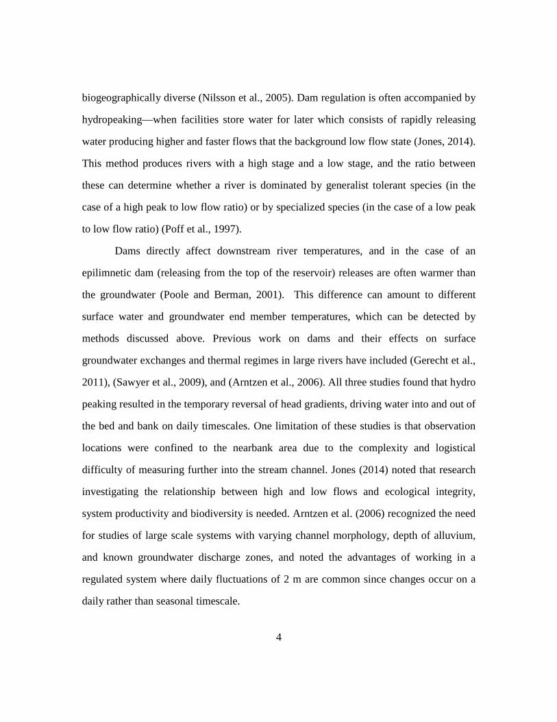
biogeographically diverse (Nilsson et al., 2005). Dam regulation is often accompanied by
hydropeaking—when facilities store water for later which consists of rapidly releasing
water producing higher and faster flows that the background low flow state (Jones, 2014).
This method produces rivers with a high stage and a low stage, and the ratio between
these can determine whether a river is dominated by generalist tolerant species (in the
case of a high peak to low flow ratio) or by specialized species (in the case of a low peak
to low flow ratio) (Poff et al., 1997).
Dams directly affect downstream river temperatures, and in the case of an
epilimnetic dam (releasing from the top of the reservoir) releases are often warmer than
the groundwater (Poole and Berman, 2001). This difference can amount to different
surface water and groundwater end member temperatures, which can be detected by
methods discussed above. Previous work on dams and their effects on surface
groundwater exchanges and thermal regimes in large rivers have included (Gerecht et al.,
2011), (Sawyer et al., 2009), and (Arntzen et al., 2006). All three studies found that hydro
peaking resulted in the temporary reversal of head gradients, driving water into and out of
the bed and bank on daily timescales. One limitation of these studies is that observation
locations were confined to the nearbank area due to the complexity and logistical
difficulty of measuring further into the stream channel. Jones (2014) noted that research
investigating the relationship between high and low flows and ecological integrity,
system productivity and biodiversity is needed. Arntzen et al. (2006) recognized the need
for studies of large scale systems with varying channel morphology, depth of alluvium,
and known groundwater discharge zones, and noted the advantages of working in a
regulated system where daily fluctuations of 2 m are common since changes occur on a
daily rather than seasonal timescale.

5
1.5. THE IMPORTANCE OF THE HYPORHEIC ZONE
The mixing of surface water and groundwater regulates many chemical reactions
in the streambed. Findlay (1995) broadly defines the hyporheic zone as the sediments that
are directly hydrologically linked to the open stream channel while Poole and Berman
(2001) define it as the portion of the alluvial aquifer that contains at least some hyporheic
groundwater. Their definition of hyporheic groundwater is water that enters the alluvial
aquifer from the stream and travels along localized subsurface flow pathways for
relatively short periods of time without leaving the alluvial aquifer.
Hydropeaking encourages mixing and changes in the thermal regime of
subsurface sediments. The work done by Gerecht et al. (2011), Sawyer et al. (2009) and
Arntzen et al. (2006) demonstrated some of these effect. Additionally, they showed that
gradient reversals occur throughout hydropeaking events, inducing a change in flow
direction. These studies also demonstrated that groundwater upwelling can limit the
extent of the hyporheic zone.
An ecotone is a transitional zone between two environments, and the hyporheic
zone represents the transition between slow moving, nutrient deplete, and temperature
stable groundwater and fast moving, nutrient rich, and dynamic surface water. In the
hyporheic zone typically the bulk of microbial biomass is in biofilms within sediment
(Boano et al., 2014). Hancock (2002) notes the importance of this ecotone as it hosts
unique invertebrate fauna and intense biogeochemical activity. Findlay (1995) expands
on this concept by introducing the idea that residence times of surface water in the system
increase by hyporheic mixing. The additional time spent in the river bed allow more time
for reactions to take place. A study done by Trauth et al., (2018) found that the highest
rates of denitrification occur when infiltrated river water fraction and hyporheic

6
temperatures are high, and determined that interactions between rivers and groundwater
are likely key controls on nitrate removal.
The chemical gradient in the hyporheic zone is one from oxic surface water near a
downwelling zone where river water infiltrates, to anoxic groundwater conditions along
deeper portions of a flow path. At the end of its path, reintroduction to the surface mixes
the now anoxic (or partially anoxic) hyporheic waters with oxic surface waters. This
distribution of oxygen implies renewal of biologically produced organic carbon (as
opposed to carbon locked up in minerals) at depth, as the uptake of O2 implies the
presence of microbial organisms (Findlay, 1995). Strong redox gradients occur at in the
interface between surface and groundwater due to microbial activity. In the hyporheic
zone typically the bulk of microbial biomass is in biofilms within sediment (Boano et al.,
2014). Oxygen is used biologically as a terminal electron acceptor (TEAP) during
respiration of organic matter, and as it is depleted, microbial communities that can use
other TEAPs such as nitrate, manganese, and iron flourish. This causes a mosaic of
electron acceptors and donors to exists that are spatially and temporally heterogeneous
and in flux with the constantly changing conditions in the hyporheic zone (Dahm et al.,
1998).
Hyporheic zone development potential is a function of channel water hydraulics
and groundwater hydraulics (White, 1993) which can be influenced by temperature and
pressure differences induced by dam regulations. These factors enforce the necessity of
understanding the changing physical and chemical characteristics that results from dam
regulation yet hyporheic zones in large rivers remain understudied due to the logistical
difficulties in instrumenting and data collection on meaningful scales. Several workers
have acknowledged the need for more studies describing the role that river stage changes
7
have on the mixing of surface water and groundwater in the riverbed (Vervier et al.,
1992;Curry et al., 1994 ;Gerecht et al., 2011).
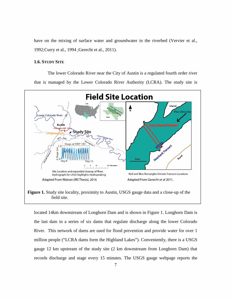
1.6. STUDY SITE
The lower Colorado River near the City of Austin is a regulated fourth order river
that is managed by the Lower Colorado River Authority (LCRA). The study site is
located 14km downstream of Longhorn Dam and is shown in Figure 1. Longhorn Dam is
the last dam in a series of six dams that regulate discharge along the lower Colorado
River. This network of dams are used for flood prevention and provide water for over 1
million people (“LCRA dams form the Highland Lakes”). Conveniently, there is a USGS
gauge 12 km upstream of the study site (2 km downstream from Longhorn Dam) that
records discharge and stage every 15 minutes. The USGS gauge webpage reports the
Figure 1. Study site locality, proximity to Austin, USGS gauge data and a close-up of the field site.

8
watershed draining 71,500 km2 upstream of the gauge and shows the river stage at this
location had daily fluctuations of least 1.5 meters throughout the summer of 2017 due to
dam operations (U.S. Geological Survey, 2018). The dam is an epilimnetic spill-over
design that empties the shallow, dammed Lady Bird Lake near Austin, Texas. Because of
this design, the water released from the dam is warm, ranging from 26-30 °C during the
summer. During the summer months, when this study was conducted, there is typically a
large contrast of 7-10 °C between the surface water and groundwater temperatures. This
combination of proximity to a hydropeaked dam, large temperature difference between
surface and groundwater, and large catchment size makes the lower Colorado River an
ideal natural laboratory for investigating the effects of hydropeaking on surface and
groundwater interactions in a large river.
2. Methods
2.1. DEPTH PROFILE TEMPERATURE DETECTORS
The primary tool used for this study was a custom-built 1-D vertical temperature
detector (Figure 2) that enabled the recording of subsurface temperature data at high
spatial and temporal resolution. The 1-D profile detectors were designed with four
sensors spaced across a 50 cm distance and were set to record temperature data every 5
minutes. TMC-HD6 air/water/soil temperature sensors were utilized, which have been
used in other SW-GW interaction studies (Gerecht et al., 2011; Nowinski et al.,
2012;Swanson and Cardenas, 2010) because they are reliable and cost-effective. Each of
the four separate temperature sensors were attached with electrical tape to a .635 cm
diameter and ~60 cm length aluminum rod (c) with the sensor tips at fixed intervals of
0.1, 0.2, 0.3 and 0.5 m from a designated 0 (e) marked on the rod with tape. The sensor
tips were left exposed and un-taped (b) so that they could measure temperature

9
effectively and accurately. Following this method, twenty-five profile detectors were
constructed for deployment in both across channel and near bank transects. The four
cables were taped together for neatness and ease of deployment (d). Each of these four
cables connected to a Hobo U12-008 four channel Data Logger (a in Figure 2) that stored
the temperature data recorded by each of the sensors. Figure 2 illustrates the
configuration of a completed 1-D detector.
The Hobo U12-008 data loggers have a reported logger accuracy of ± 2 mV ± 1%
of reading for data logger-powered sensors with a resolution of 0.6 mV and an operating
range of -20 to 70 °C (“HOBO U12 4-Channel External Data Logger - U12-008”). When
connected to the U12 data loggers the TMC-HD6 temperature sensors have a
measurement range of -40 to 50 °C in water with an accuracy of ±0.25°C from 0° to
50°C, a resolution of 0.03° at 20°C (0.05° at 68°F), and drift of <0.1°C/year. The
Figure 2. Annotated image of Depth Profile Temperature Detector. Letters following components correspond to in text descriptions.

10
response time of the temperature sensors is 30 seconds in stirred water (“Air Water Soil
Temp Sensor (6’ cable) | Onset HOBO”).
2.2. CROSS CHANNEL TRANSECT
The main research objective of this study involved collecting detailed temperature
data across the entire width of the channel at the study site to see how the hyporheic zone
thermal regime responded to the daily hydropeaking releases. The large size of the
channel (68 m in width) and rapid daily changes in flow due to hydropeaking made data
collection technically and logistically challenging. Two significant challenges included
installing the temperature detectors and their cables securely enough that they wouldn’t
be damaged during high flow periods, and the short time windows when daylight and
flow conditions allowed for working safely in the river. Spanning the river channel with
instrumentation required low-profile design to ensure there was no obstruction of
navigability or loss of instruments and data due to debris moving downstream during
hydropeaking releases.
2.2.1 Cross Channel Transect: Temperature Profile Arrays
The limitations on deployment required pre-fabricating arrays that could be fixed
to the bottom of the river before the steep daily stage increase around 12 pm. To
accomplish this, six temperature arrays were constructed from twenty-four depth profile
temperature detectors. The loggers and their associated depth profile temperature
detectors were given ID’s and organized in ascending order with different colored tape
marking each end of the array to ensure deployment in ascending order. Depth profile
temperature detectors (a) were spaced 2.75 m apart and the bundles of 4 cables were

11
taped together. Sand stakes (b) were attached to the cable bundles in-between each depth
profile temperature detector so that upon deployment the cable bundles could be fixed to
the river bottom and would not entrain or entangle recreational boaters or debris. The
data loggers were cable tied in sets of two (c), and the two resulting groupings were
loosely cable tied so that upon deployment they could be tightened to a T post in the
riverbed (d). The center point of each array consisted of a T-post that served as an anchor
for the loggers. Excess cable was bundled and taped into a loop (e) that could be placed
over the T-post. This configuration is displayed in Figure 3.
Figure 3. Annotated image showing temperature detecting array and a close up of the data loggers. (c) shows the 4 loggers cable tied together, (d) is a T post

12
To install the arrays in a straight line, a rope was stretched taught perpendicular to
flow across the river to serve as a guide. Equipped with a weight belt and snorkel, the
researcher manually installed the arrays into the riverbed with a post driver. After the first
two 1-D profiles in an array were installed, the T-post was driven into the bed and the
loops of bundled cable were placed over the post. The data loggers were cable tied to the
T-post and the remaining two depth profile temperature detectors and their associated
stakes were driven into the river bed. This process was repeated to install all of the depth
profile temperature detectors 2.75 m apart spanning the 68 m from bank to bank at low
stage with temperature sensors at 0.1, 0.2, 0.3, and 0.5 meters depth. Three of the depth
profile temperature detectors (shown at approximately 49 m, 56 m, and 58 m) could not
be driven to depth because a hard relatively impermeable clay layer was present at just
over 0.3 m depth, the sensor tips at these locations were instead at 0, 0.1, and 0.3 depths.
The precise locations of each depth profile temperature detector were surveyed using a
13
Sokkia theodolite set 610 with an accuracy of 6 degree seconds (SOKKIA Series 10
Operator’s Manual, 2001). The data logger’s clocks were synchronized and set to record
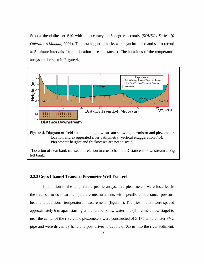
at 5 minute intervals for the duration of each transect. The locations of the temperature
arrays can be seen in Figure 4.
2.2.2 Cross Channel Transect: Piezometer Well Transect
In addition to the temperature profile arrays, five piezometers were installed in
the riverbed to co-locate temperature measurements with specific conductance, pressure
head, and additional temperature measurements (figure 4). The piezometers were spaced
approximately 6 m apart starting at the left bank low water line (shoreline at low stage) to
near the center of the river. The piezometers were constructed of 3.175 cm diameter PVC
pipe and were driven by hand and post driver to depths of 0.5 m into the river sediment.
Figure 4. Diagram of field setup looking downstream showing thermistor and piezometer location and exaggerated river bathymetry (vertical exaggeration 7.5). Piezometer heights and thicknesses are not to scale.
*Location of near bank transect in relation to cross channel. Distance is downstream along left bank.
14
The PVC was screened from 0.4-0.5 m depth. The top-of-casing piezometer positions and
riverbed surface elevations were surveyed using the Sokkia Theodolite Set 610. Each
piezometer was instrumented with a Solinst Level Logger LTC M30 that measured
specific conductance, temperature, and depth. Prior to deployment, the Solinst LTC M30
level loggers were calibrated to an accuracy of ±2% within the range of 500 - 30,000
μS/cm. The instrument accuracy for depth is ± 1.5 cm, and for temperature ±0.05ºC
(“LTC Levelogger Edge”). The data logger’s clocks were synchronized and set to collect
data every 5 minutes. An In-Situ BaroTroll data logger was deployed at the field site to
collect atmospheric temperature and pressure readings throughout the time of the study
and these were subtracted from the transducer pressure readings from the piezometers so
that observed changes in pressure only reflected changes in river stage. An additional
monitoring well on the bank constructed of 3.175 cm diameter PVC pipes screened below
the land surface and extending well into the water table was instrumented with a Solinst
LTC M30 level logger. This well was used to determine average groundwater
temperature and electrical conductivity.
2.2.3. Cross Channel Transect: Water Flux Estimates
Hydraulic conductivity estimates of the shallow river sediment at the field site
were available from unpublished work that collected sediment samples co-located with
the temperature and piezometer transect. Grain size analysis was conducted for each of
the sediment samples and was used to empirically-derive K (hydraulic conductivity)
values for each of the samples (Martinez 2017). The K values utilized to calculate q
(specific discharge) were derived from sediment samples that were taken every 2.5m
across the river at the river bed and determined using the Hazen method (Hazen, 1983).

15
While the samples were only collected at the surface and may not be completely
representative of the 0.5 m of underlying sediment, the fluxes calculated should be
considered as approximations that are likely within an order of magnitude, and
importantly, this uncertainty does not affect estimates of flow direction. To calculate
specific discharge, vertical hydraulic gradient is needed in conjunction with estimated
hydraulic conductivity. Vertical hydraulic gradient was determined by the following
equation. 𝑉𝑉𝑉𝑉𝑉𝑉 = 𝑅𝑅𝑅𝑅𝑅𝑅𝑅𝑅𝑅𝑅 𝑑𝑑𝑅𝑅𝑅𝑅𝑅𝑅𝑑𝑑−𝑃𝑃𝑅𝑅𝑅𝑅𝑃𝑃𝑃𝑃𝑃𝑃𝑅𝑅𝑡𝑡𝑅𝑅𝑅𝑅 𝑑𝑑𝑅𝑅𝑅𝑅𝑅𝑅𝑑𝑑
0.4𝑃𝑃 (3)
Where VHG is vertical hydraulic gradient and .4 meters is the distance from the sediment
water interface to the top of the screened interval. The flux was determined from a
modified Darcy’s law considering only vertical components of specific discharge.
Equation 4 is a modified version of equation 1 shown in the introduction, where the
pressure gradient is replaced with the vertical hydraulic gradient
𝑞𝑞 = −𝑘𝑘(𝑉𝑉𝑉𝑉𝑉𝑉) (4)
This calculation assumes one dimensional flow and does not account for multi-
dimensional flow pathways. Still, it is useful in demonstrating overall flow direction and
whether the river is gaining or losing water across both time and space.
2.2.4. In Stream Measurements
To measure stage and temperature, an Aqua Troll 200 was deployed in the river.
The Aqua Troll 200 recorded temperature and pressure (depth) every 15 minutes. The
temperature accuracy is ±0.1° C. with a resolution of 0.01° C or better and the depth
accuracy is ±0.175 cm.(“Aqua TROLL 200 Data Logger”)To have a second in-stream

16
measurement of temperature, an Onset HOBO Water Temp Pro v2 with an accuracy of
±0.2°C was installed in the center of the channel cable tied to one of the T-Posts installed
for the temperature sensing arrays(“HOBO Water Temperature Pro v2 Data Logger”). It
logged measurements every 5 minutes.
2.3 NEARBANK TRANSECT
While this study primarily focused on the cross-channel effects of hydropeaking,
the effects of hydropeaking on the near-bank hyporheic zone were also investigated.
Observational (Gerecht et al., 2011) and numerical modeling studies (Wilson and
Gardner, 2006; Gardner and Wilson, 2006; Shuai et al., 2017) have shown that the near-
bank experiences the most significant flow changes during rising and falling stage, and
suggest that this area may have disproportionate importance for net exchange during
hydropeaking events. This motivated the creation of a near bank transect. The near-bank
transect was easier to install because of its location out of the main flow of the river. Data
loggers could be fixed onshore where debris and boaters would not disturb them. Its
location relative to the river bank and the cross-channel transect is shown in Figure 4
(blue dots).
2.3.1 Near-bank Transect: Temperature Profile
Seventeen depth profile temperature detectors measured riverbed temperatures at
0.1, 0.2, 0.3 and 0.5 m depths approximately 1.5 m from the bank (here bank is used to
mean the near vertical component of the river bank where it steepens dramatically). The
transect spanned ~16 m going downstream. After the first depth profile temperature
detector was installed 1.5 m from the bank, 1 m was measured downstream and then that

17
point was adjusted so that it would be 1.5 m from the bank at that location. The excess
cables were bundled and placed on shore around T-posts.
2.3.2 In Stream Measurements
To measure stage and temperature, an Aqua Troll 200 was deployed in stream and
cable tied and taped to a T-post driven into the stream-bed. The level logger recorded
temperature, pressure and depth every 15 minutes.
2.4 DATA PROCESSING
Overall, the temperature data for both transects was of high quality with few
instances of inaccurate or imprecise data, which typically resulted from damage to the
sensors or cable during installation. Spikes in the temperature data (erroneous
measurements) were uncommon, easy to identify, and filtered out manually. In the wells,
conductivity and temperature data required no filtering or smoothing, but pressure data
had some noise. The temperature data were visualized and analyzed using Mathworks
Matlab to grid, interpolate, and plot the data. In Figures 7 and 11 for visualization
purposes a median filter was utilized (matlab function medfilt1). Median filters smooth
out noise by going element by element and replacing them with the median of
surrounding elements. Additionally, linear 2-D interpolation was utilized to interpolate
temperatures between measured points and create a 2-D visualization of hyporheic zone
temperature. The boxplots in Figures 6 and 10 only had spikes removed and remained
unfiltered. For specific discharge calculations, vertical hydraulic gradient was smoothed
using a moving average (Matlab function tsmovavg) with a window set to 10 increments.
Moving averages were utilized because the pressure data had some noise, this noise is

18
hypothesized to have come from the wells vibrating slightly with current flowing around
them, as the fluctuations are not seen in the temperature or conductivity data. The moving
average smoothed out the data by replacing each element with the average of the 10
elements surrounding it.

19
3. Results and Discussion
3.1 CROSS-CHANNEL TEMPERATURE PROFILES
Subsurface temperature data for the cross-channel transect was collected over an
8-day period from 7/20-7/28 2017. The river was hydropeaked continuously over this
period with daily stage fluctuations of 1-1.25m (Figure 5). During the study stream
temperature was warm and had a narrow temperature range from 26.91°C to 30.70 °C
while the subsurface temperatures of the shallow stream sediments had a wider range in
Figure 5. Four temperature depth profile time series across the river compared to stage change for 8 days throughout the study. The temperature fluctuations have differing magnitudes depending on their location, but the fluctuations in temperature all coincide with changes in stage. Right Panel Adapted from Gerecht et all 2011.

20
temperatures 20.53°C to 30.37°C, spanning the range of the groundwater and surface
water thermal regimes. Qualitatively, the temperatures in the hyporheic zone appear to
co-vary with changes in stage throughout the course of the study, and showed consistent
responses day to day supporting the hypothesis that stage fluctuations cause changes in
subsurface temperatures. Figure 5 shows temperature profiles at four different locations
across the river and demonstrates the stage induced forcing of daily temperature
fluctuations. At increasing depth in the river the temperature and magnitude of the change
is smaller, and further across the river there are smaller changes in daily temperature. At
location A, nearest the bank the thermal signal is seen at all depths, while at B, C and D
the temperature signal is recorded in the top .3 m. Work done by Gerecht et al., (2011)
demonstrated that at the study site, signature penetration by conduction alone could only
reach .15 m. These results therfore support advective heat transport driven by fluid flow
at all locations.

21
To concisely summarize the time series temperature data for all of the cross-
channel data, daily ranges were calculated for all four sensors at each of the 21 locations.
The calculated range (max-min daily temperature) for all of the data is summarized in
Figure 6A: Daily temperature ranges for seven days and different depths plotted against distance from the left bank. The deeper in the subsurface, the less temperature fluctuates at each location.
Figure 6B: Boxplots of temperature for 2 days (7/26-27/17) at each location across the channel. The blue lines represent the boundary minimum and maximum of surface water temperatures and the tan lines represent boundary minima and maxima of the groundwater discharge temperature range at 0.5 m depth.

22
Figure 6. Figure 6a shows the ranges. At 0.1 m depth the average fluctuation is 1.28 °C
with a standard deviation of 1.4 °C and a maximum fluctuation of 6.7 °C. At 0.2 m depth
the average fluctuation is .97°C with a standard deviation of 1.29°C and at 0.3 m depth
the average fluctuation is 0.53°C with a standard deviation of 0.72°C. At 0.5 m depth the
minimum fluctuation is 0.03 °C and the average across the river is 0.18 °C with a
standard deviation of 0.21 °C. Within 12 m from the left back the fluctuations at all
depths are higher. Isolating locations closer than 12 m at 0.1 m depth the average
fluctuation is 4.10 °C with a standard deviation of 1.84 °C and at 0.5 m depth the
temperature fluctuates an average of 0.72 °C with a standard deviation of 0.13°C. Beyond
12m, the subsurface temperature ranges are similar to one another with all standard
deviations falling below 0.27 °C Figure 6A demonstrates these trends.
Ranges in temperatures indicate the magnitude of fluctuations at each location but
do not identify the surface or ground water as the dominant forcing. A way to show the
range of subsurface temperatures relative to groundwater and surface water end members
is using boxplots to summarize the temperature data at each location. Figure 6b compiles
two days of data, eliminating the exaggerated range displayed if all the data is displayed
due to daily changes in ambient temperature. Looking at this figure, the relative influence
of surface water and groundwater on the subsurface temperatures can be seen. The box
plots demonstrate that beyond 19 m from shore, surface water influences the subsurface
temperatures because subsurface temperatures lie entirely within the surface water range.
Within 19 m, the temperature ranges indicate both surface water and ground water
temperatures influence subsurface temperatures on daily scales. The fact that the daily
ranges span both the groundwater discharge and surface water temperature ranges
suggests groundwater-surface water mixing on daily timescales. In summary, the
subsurface temperatures across the channel vary from a small range of higher

23
temperatures matching surface water temperatures further than 19 m from the shore to a
wider range from high to low temperatures closer to the shore.
In between hydropeaks, colder water that is the near the endmember temperature
of ground water rises to the surface within 12 m. Between 12 m and 19 m from the shore,
there are some intermediate temperatures, while further than 19 m, the temperature of the
sediments remain consistently warm. During a hydropeaking cycle (defined as low stage
to high stage back to low stage), locations within 19 m of the bank show subsurface
temperatures respond to and experience varying proportions of the endmember
temperatures. At the initiation of a hydropeak, the subsurface temperatures are similar to
the resting distribution of temperatures. As the hydropeak progresses there is a rapid
increase in temperatures near the bank, and soon after the hydropeak the temperatures in
the first 0.5 m as measured all exhibit influence from surface water. Afterwards the
cooler groundwater temperatures return at the locations near the bank. This rapid
disappearance of the warm surface water temperatures near the bank implies a
resumption of groundwater upwelling. Further into the channel, the temperatures remain
consistently warm and there are only subtle changes in hyporheic sediment temperatures
throughout the course of a hydropeak. This is demonstrated in figure 7. At the right
bank, the upwelling, cooler signal is not seen. This likely indicates a deeper groundwater
table and potential losing conditions locally.

24
Figure 7. 2D temperature profiles across the river throughout the course of a hydro peaking event. T1 shows low stage and the steady resting distribution of temperatures. T2 and T3 show the temperature distributions just before a hydropeak. T4 shows just after a hydropeak. T5 is a return to steady resting distribution of temperature. The temperature increases in the subsurface is most extreme near the bank in T4, while through all time steps the sediments beyond 12 m see little change.
25
Differing temperature responses to hydropeaking were based on location and are
demonstrated in both the range and temperature time series analysis. Temperature ranges
were high and influenced by both surface and groundwater near the left bank, yet
diminished to surface water ranges across the width of the river. The right bank did not
show influence from groundwater temperatures. Jackson et al., (2007) and Hill and
Hawkins (2014) both state temperature’s importance in determining benthic
macroinvertebrate assemblage and widescale studies determining the effect of different
stressors on macroinvertebrate assemblages utilize stream temperature as a variable
(Meador et al., 2008; Carlisle et al., 2007). Beyond macroinvertebrate assemblages,
temperature is a controlling factor for nutrient processing associated with microbial
communities and biofilms (Boano et al., 2014). These findings show that over the course
of 8 days with a stream temperature range of 3.9°C subsurface temperatures experience a
much larger range of 9.83°C. Stream temperature remains an important variable, but in
hydropeaked gaining systems the range of temperature in the river will usually be smaller
than the range of temperatures in the nearbank benthic habitat. This implies that as an
environmental indicator, surface water temperatures may be insufficient for determining
aquatic habitat suitability in hydropeaked systems, especially for benthic
macroinvertebrates and hyporheic biofilms which reside in the subsurface. Gradients of
nutrient and chemical availability will be highly changing and evolving near the bank and
discharge zones, while further in the river temperatures are more static despite large stage
fluctuations.

26
3.2 ACROSS CHANNEL IN-STREAM PIEZOMETER DATA
Wells in the stream provided head, conductivity, and temperature data to
corroborate with the temperature data obtained in cross section. In some cases, the
additional chemical and conductivity measurements revealed patterns not demonstrated
through temperature alone. Using pressure head data in the piezometers with head from
the river surface elevation, vertical head gradients were calculated to estimate vertical
flux rates.
Locations near the bank experienced flux and gradient reversals that co-varied
with river stage. The only two locations that experienced gradient reversals and a change
in the direction of flux from into the bank to out of the bank were at 0.56 and 6.9 m.
Beyond this distance, the gradients and fluxes did not change with stage, and remained
relatively constant throughout each hydropeaking event. The largest positive (out of
bank) and negative (into bank) fluxes were measured at 6.9 m from the shore, with fluxes
Figure 8. Estimated fluxes throughout the course of 2 flood pulses. Two Locations near the bank (0.56 and 6.9 m) experienced flux and gradient reversals that co varied with river stage. The remaining 3 wells did not change with stage, and remained relatively constant throughout the course of the study. This pattern is consistent with the thermal data presented in figure 7 and the electrical conductivity presented in figure 8 which show similar spatial trends of response to stage.

27
out of the bank reaching 10 m/d specific discharge (also known as Darcy flux) and
dropping to nearly -3 m/day. Sediments near the bank recorded much smaller discharge
despite a higher vertical head gradient due to lower hydraulic conductivity values. These
results are presented in Figure 8. At the study site, groundwater and surface water have
different specific conductance values. Throughout the course of the study, the
groundwater well in the bank measured an average of 1237 µS/cm. The river, while well
homogenized at any given instant, has a specific conductance that varies through time.

28
Other workers at this field site have found the average specific conductance of the river
to be 550 µS/cm (Stephen Ferencz, Personal Communication). Using these values as pure
groundwater and pure surface water endmembers in a ratio allowed the conductivity
values collected in the river piezometers to determine the percent contribution of each
endmember during hydropeaking events. This calculation is a rough approximation, as it
assumes constant and unchanging conductivity values for the groundwater and surface
water endmembers. Additionally the water previously in the piezometer is mixing with

29
the water coming in through the slots as it changes in the sediments, and is therefore only
an approximate measure of the specific conductance at any given time. While a well in
the bank was utilized to determine an average groundwater specific conductance, the
highest measured specific conductance was actually in one of the river piezometers and
was 1287 µS/cm for the period shown, so this value was used for a pure groundwater
endmember. Figure 9 shows the results from this end-member analysis. At 0.5 and 7
meters from the bank, flood pulses cause a mixing of surface and groundwater, and each
Figure 9. Relationship between specific conductance (percent groundwater assuming pure GW specific conductance = 1287 µS/cm and surface water specific conductance =550 µS/cm), temperature, and stage for the 5 piezometers located from .56 m from the bank to 25.76 m into the river. Specific conductance values indicate mixing, as well as some trends that are not displayed in the thermal data. Wells A and B are anti-correlated with stage changes, demonstrating surface water infiltration into the subsurface near the bank at high stage. Well C does not vary with stage change and is almost purely groundwater, while well D co varies with stage but rises to a higher percent groundwater which is the opposite of what is expected. Well E is nearly all surface water all the time, and does not vary with t
30
location goes from being predominantly groundwater to predominantly surface water.
This is shown in the temperature profile data. The well at 13 m has a relatively constant
electrical conductivity, and is close to 100% groundwater at all times. The only exception
are small dips at low stage prior to a hydropeak.
At 19 m, an unexpected pattern is displayed where rise in conductivity and
groundwater percent are seen with a rise in stage. Lastly, at 26m the hyporheic water is
nearly all surface water, and sees no effects of the hydropeak. While this end-member
analysis is a coarse estimate, it shows bulk behavior of hyporheic composition and degree
of GW-SW mixing in response to hydropeaking events.
In addition to providing estimates of GW-SW mixing, the pressure data from the
piezometer measurements help explain the difference in temperature responses observed
across the channel. Pressure gradients and fluxes reverse throughout flood pulses within
12 m from the bank, while further out, there is a minimal change in head gradients
despite large fluctuations in stage. Time varying loading in an aquifer results in changing
stresses on the aquifer, and can lead to diminished recharge because of increasing pore
pressure due to surficial load (Reeves et al., 2000). This has been extensively documented
in tidal systems (Befus et al., 2013; Cardenas et al., 2015; Reeves et al., 2000; Gardner
and Wilson, 2006) and recent work has shown the concept applied to freshwater systems
(Shuai et al., 2017). Modeling based on the study site incorporating this loading effect
have shown results consistent with our field observations and temperature and head
gradients measured in this study serve as evidence for this process (Shuai et al., 2017).
Changes in stage drive exchange near the banks while across the river despite dynamic
conditions loading results in largely static gradient and flow conditions in the bed.
Measuring electrical conductance demonstrates patterns not seen in the pressure and
temperature fields, and while these measurements were not a main focus of the study,

31
they likely demonstrate the presence of multiple flow regimes and non-vertical and one
dimensional flow fields. The measurement in the piezometer at 19 m demonstrates a
trend that would not be seen in only temperature data, as in the well during a hydropeak
temperatures rise with the river fluctuation, yet instead of low conductivity values high
values are measured. This demonstrates what could be interpreted as hyporheic
groundwater with a longer residence time and non-vertical flow pathway that remains in
the bed long enough to be warmed up through conduction.
3.3 NEAR BANK TEMPERATURE PROFILES
Near bank temperatures 1.5 m from the left shore followed the trend observed in
the cross channel transect of decreasing range with depth. At 0.5 m depth the minimum
fluctuation is 0.09 °C and the average across the river is 1.84 °C with a standard
deviation of 0.7 °C. In contrast, at 0.1 m depth the average fluctuation is 5.77 °C with a
standard deviation of 0.95°C and a maximum fluctuation of 7.4 °C. These values fit in
with the trends observed in Figures 6a and 6b.The near bank values also fit the trend of
increasing range with proximity to the bank. There are no observable trends/differences
moving downstream, which validates the cross channel transect as representative of this
reach of river on the scale of meters up and downstream. The data is displayed in Figure
10a. Figure 10b displays the data for 2 days in boxplots grouped by location. Each
boxplot extends from within the groundwater range into the surface water range, which
indicates influence from both the surface water and ground-water temperatures. The
boxplots display no trends moving downstream, and compared to figure 6b fit in the trend
set and would plot as expected from the across channel investigation due to their distance
from the shore.

32
The subsurface temperatures near the bank throughout the course of a hydropeak
show uniform response moving downstream, and the penetration of the thermal signal
Figure 10 A: Daily temperature ranges for 6/22-26/17 at four depths 1.5 m from the shore moving downstream along the bank. The ranges matches the trends found in plot 6a and 6b as all of these locations are closer to the bank and display the same large range consistent with being near the bank. There is a consistent scatter to the points, suggesting that there are no differing trends moving downstream. There is a consistent trend of decreasing range with depth.
Figure 10 B: Box plots of temperature range moving downstream 1.5 m from the bank. The blue lines represent the boundary minimum and maximum of surface water temperatures, the tan lines represent boundary minima and maxima of the groundwater discharge temperature range at .5 m depth. The boxplots extend through both ranges in all cases, which indicates influence of both surface water and groundwater in the first .5 m at all locations.

33
reaches all the way to 0.5 m depth. In between peaks, cool groundwater endmember
temperatures dominate the subsurface temperatures. Figure 11 shows snapshots of the
subsurface temperatures throughout the course of a hydropeak, demonstrating the
penetration of warm surface water signals into the subsurface, and the recovery of cooler
temperatures matching cooler groundwater signals.
Figure 11. Shows 2D temperature profiles at different time slices along the bank 1.5 m from the shore moving downstream. The temperature distributions follow the trend established across channel transect shown in figure 7, of reversals of flow and surface water infiltration with proximity to the bank. T1 shows between hydropeaks, with cool groundwater dominating the subsurface temperature profile. T2 is just after a peak showing some infiltration, T3 is at a peak and has surface water temperatures affecting nearly the entire first 50 cm of the subsurface, T4 is the tail of a hydropeak and shows cool groundwater temperatures returning, and T5 is at the end of a hydropeak and shows a temperature distribution similar to that in T1.

34
The downstream transect demonstrated consistency and minimal changes in
temperature response as a function of distance downstream. Since pressure measurements
explained differences in temperature, it can be inferred that the findings are not isolated
to the 2d cross section, but can be generalizable upstream and downstream as well.

35
4. Conclusions
The effects of hydropeaking on the temperature regime and surface and
groundwater interactions in a large regulated river were investigated by measuring two
temperature depth profiles, one near the bank moving downstream and the other across
the width of the river. Piezometers allowed for the additional measurement of head
gradients and specific conductance measurements of hyporheic water. Near a gaining
bank hydropeaking induces increased temperature ranges and groundwater surface water
interactions while further away from the bank temperature profiles and pressure gradients
remain more close to static. Results from this study indicate measurements of surface
water temperature alone may not be sufficient to show disturbance from hydropeaking as
temperature ranges are higher in the streambed than in the river, which is an important
ecotone and a biologically significant component of the system. Flux and gradient
reversals explain the temperature distribution and are consistent with findings
investigating loading effects in intertidal zones, where the weight of water associated
with tidal increase is analogous to the rapid stage change caused by hydropeaking. This
effect has been successfully incorporated into models at the study site, and the model
results match physical observations. Electrical conductivity data suggests the presence of
multiple scales of flow pathways, revealing patterns not seen in temperature profiles.
Down-stream results indicate that cross channel observations can be extrapolated
downstream on m scales despite the high prevalence of heterogeneity in the river. Future
recommendations in the investigation of hyporheic zones and dam regulation include
investigations further quantifying microbial and benthic macroinvertebrate assemblage
and response to the presence of static and dynamic habitat created by hydropeaking, as

36
well as investigation into signals of the multi-dimensional flow components of hyporheic
exchange.

37
Works Cited
Air Water Soil Temp Sensor (6’ cable) | Onset HOBO, http://www.onsetcomp.com/products/sensors/tmc6-hd (accessed February 2018).
Allan, J.D., and Castillo, M.M., 2007, Stream Ecology: Structure and function of running waters: Springer Netherlands, //www.springer.com/us/book/9781402055829 (accessed February 2018).
Anderson, M.P., 2005, Heat as a Ground Water Tracer: Ground Water, v. 43, p. 951–968, doi: 10.1111/j.1745-6584.2005.00052.x.
Aqua TROLL 200 Data Logger In-Situ, https://in-situ.com/products/water-level-monitoring/aqua-troll-200-data-logger/ (accessed February 2018).
Arntzen, E.V., Geist, D.R., and Dresel, P.E., 2006, Effects of fluctuating river flow on groundwater/surface water mixing in the hyporheic zone of a regulated, large cobble bed river: River Research and Applications, v. 22, p. 937–946, doi: 10.1002/rra.947.
Befus, K.M., Cardenas, M.B., Erler, D.V., Santos, I.R., and Eyre, B.D., 2013, Heat transport dynamics at a sandy intertidal zone: Water Resources Research, v. 49, p. 3770–3786, doi: 10.1002/wrcr.20325.
Boano, F., Harvey, J.W., Marion, A., Packman, A.I., Revelli, R., Ridolfi, L., and Wörman, A., 2014, Hyporheic flow and transport processes: Mechanisms, models, and biogeochemical implications: Reviews of Geophysics, v. 52, p. 603–679, doi: 10.1002/2012RG000417.
Burkholder, B.K., Grant, G.E., Haggerty, R., Khangaonkar, T., and Wampler, P.J., 2008, Influence of hyporheic flow and geomorphology on temperature of a large, gravel-bed river, Clackamas River, Oregon, USA: Hydrological Processes, v. 22, p. 941–953, doi: 10.1002/hyp.6984.
Cardenas, M.B., Bennett, P.C., Zamora, P.B., Befus, K.M., Rodolfo, R.S., Cabria, H.B., and Lapus, M.R., 2015, Devastation of aquifers from tsunami-like storm surge by Supertyphoon Haiyan: Geophysical Research Letters, v. 42, p. 2844–2851, doi: 10.1002/2015GL063418.
Carlisle, D.M., Meador, M.R., Moulton, S.R., and Ruhl, P.M., 2007, Estimation and application of indicator values for common macroinvertebrate genera and families of the United States: Ecological Indicators, v. 7, p. 22–33, doi: 10.1016/j.ecolind.2005.09.005.
Chapra, S.C., 2008, Surface water-quality modeling: Long Grove, IL, Waveland press. Conant, B., 2004, Delineating and quantifying ground water discharge zones using
streambed temperatures: Ground Water, v. 42, p. 243–257, doi: 10.1111/j.1745-6584.2004.tb02671.x.

38
Curry, R., Gehrels, J., Noakes, D., and Swainson, R., 1994, Effects of River Flow Fluctuations on Groundwater Discharge Through Brook Trout, Salvelinus-Fontinalis, Spawning and Incubation Habitats: Hydrobiologia, v. 277, p. 121–134, doi: 10.1007/BF00016759.
Dahm, C.N., Grimm, N.B., Marmonier, P., Valett, H.M., and Vervier, P., 1998, Nutrient dynamics at the interface between surface waters and groundwaters: Freshwater Biology, v. 40, p. 427–451, doi: 10.1046/j.1365-2427.1998.00367.x.
Ebersole, J.L., Liss, W.J., and Frissell, C.A., 2003, Thermal heterogeneity, stream channel morphology, and salmonid abundance in northeastern Oregon streams: Canadian Journal of Fisheries and Aquatic Sciences, v. 60, p. 1266–1280, doi: 10.1139/F03-107.
Findlay, S., 1995, Importance of surface-subsurface exchange in stream ecosystems: The hyporheic zone: Limnology and Oceanography, v. 40, p. 159–164, doi: 10.4319/lo.1995.40.1.0159.
Gardner, L.R., and Wilson, A.M., 2006, Comparison of four numerical models for simulating seepage from salt marsh sediments: Estuarine, Coastal and Shelf Science, v. 69, p. 427–437, doi: 10.1016/j.ecss.2006.05.009.
Gerecht, K.E., Cardenas, M.B., Guswa, A.J., Sawyer, A.H., Nowinski, J.D., and Swanson, T.E., 2011, Dynamics of hyporheic flow and heat transport across a bed-to-bank continuum in a large regulated river: Water Resources Research, v. 47, p. W03524, doi: 10.1029/2010WR009794.
Hancock, P.J., 2002, Human Impacts on the Stream–Groundwater Exchange Zone: Environmental Management, v. 29, p. 763–781, doi: 10.1007/s00267-001-0064-5.
Hawkins, C.P., Hogue, J.N., Decker, L.M., and Feminella, J.W., 1997, Channel morphology, water temperature, and assemblage structure of stream insects: Journal of the North American Benthological Society, v. 16, p. 728–749, doi: 10.2307/1468167.
Hazen, A., 1983, Some physical properties of sand and gravel with special reference to their use in filtration: 24th Ann, Rep., Mass. State Board of Health, Boston, 1983,.
Hester, E.T., and Doyle, M.W., 2011, Human Impacts to River Temperature and Their Effects on Biological Processes: A Quantitative Synthesis1: JAWRA Journal of the American Water Resources Association, v. 47, p. 571–587, doi: 10.1111/j.1752-1688.2011.00525.x.
Hill, R.A., and Hawkins, C.P., 2014, Using modelled stream temperatures to predict macro-spatial patterns of stream invertebrate biodiversity: Freshwater Biology, v. 59, p. 2632–2644, doi: 10.1111/fwb.12459.

39
HOBO U12 4-Channel External Data Logger - U12-008, http://www.onsetcomp.com/products/data-loggers/u12-008 (accessed February 2018).
HOBO Water Temperature Pro v2 Data Logger, http://www.onsetcomp.com/products/data-loggers/u22-001 (accessed February 2018).
Hucks Sawyer, A., Bayani Cardenas, M., Bomar, A., and Mackey, M., 2009, Impact of dam operations on hyporheic exchange in the riparian zone of a regulated river: Hydrological Processes, v. 23, p. 2129–2137, doi: 10.1002/hyp.7324.
Jackson, H.M., Gibbins, C.N., and Soulsby, C., 2007, Role of discharge and temperature variation in determining invertebrate community structure in a regulated river: River Research and Applications, v. 23, p. 651–669, doi: 10.1002/rra.1006.
Jones, N.E., 2014, The Dual Nature of Hydropeaking Rivers: Is Ecopeaking Possible? River Research and Applications, v. 30, p. 521–526, doi: 10.1002/rra.2653.
Łaszewski, M., 2016, Relationships between environmental metrics and water temperature: a case study of Polish lowland rivers: Water and Environment Journal, v. 30, p. 143–150, doi: 10.1111/wej.12173.
LCRA dams form the Highland Lakes, https://www.lcra.org/water/dams-and-lakes/Pages/default.aspx (accessed March 2018).
LTC Levelogger Edge, https://www.solinst.com/products/dataloggers-and-telemetry/3001-levelogger-series/ltc-levelogger/datasheet.php (accessed February 2018).
Meador, M.R., Carlisle, D.M., and Coles, J.F., 2008, Use of tolerance values to diagnose water-quality stressors to aquatic biota in New England streams: Ecological Indicators, v. 8, p. 718–728, doi: 10.1016/j.ecolind.2008.01.002.
Nilsson, C., Reidy, C.A., Dynesius, M., and Revenga, C., 2005, Fragmentation and Flow Regulation of the World’s Large River Systems: Science, v. 308, p. 405–408, doi: 10.1126/science.1107887.
Nowinski, J.D., Cardenas, M.B., Lightbody, A.F., Swanson, T.E., and Sawyer, A.H., 2012, Hydraulic and thermal response of groundwater–surface water exchange to flooding in an experimental aquifer: Journal of Hydrology, v. 472–473, p. 184–192, doi: 10.1016/j.jhydrol.2012.09.018.
Parkinson, E.A., Lea, E.V., Nelitz, M.A., Knudson, J.M., and Moore, R.D., 2016, Identifying Temperature Thresholds Associated with Fish Community Changes in British Columbia, Canada, to Support Identification of Temperature Sensitive Streams: River Research and Applications, v. 32, p. 330–347, doi: 10.1002/rra.2867.
40
Poff, N.L., Allan, J.D., Bain, M.B., Karr, J.R., Prestegaard, K.L., Richter, B.D., Sparks, R.E., and Stromberg, J.C., 1997, The natural flow regime: A paradigm for river conservation and restoration: BioScience, v. 47, p. 769–784.
Poole, G.C., and Berman, C.H., 2001, An ecological perspective on in-stream temperature: natural heat dynamics and mechanisms of human-caused thermal degradation: An Ecological Perspective on In-Stream Temperature journalArticle ISSN0364-152X, doi: 10.1007/s002670010188.
Rau, G.C., Andersen, M.S., and Acworth, R.I., 2012, Experimental investigation of the thermal dispersivity term and its significance in the heat transport equation for flow in sediments: Water Resources Research, v. 48, doi: 10.1029/2011WR011038.
Rau, G.C., Andersen, M.S., McCallum, A.M., Roshan, H., and Acworth, R.I., 2014, Heat as a tracer to quantify water flow in near-surface sediments: Earth-Science Reviews, v. 129, p. 40–58, doi: 10.1016/j.earscirev.2013.10.015.
Reeves, H.W., Thibodeau, P.M., Underwood, R.G., and Gardner, L.R., 2000, Incorporation of Total Stress Changes into the Ground Water Model SUTRA: Ground Water, v. 38, p. 89–98, doi: 10.1111/j.1745-6584.2000.tb00205.x.
Shuai, P., Cardenas, M.B., Knappett, P.S.K., Bennett, P.C., and Neilson, B.T., 2017, Denitrification in the banks of fluctuating rivers: The effects of river stage amplitude, sediment hydraulic conductivity and dispersivity, and ambient groundwater flow: Water Resources Research, v. 53, p. 7951–7967, doi: 10.1002/2017WR020610.
SOKKIA Series 10 Operator’s Manual, 2001, 260-63 HASE, ATSUGI, KANAGAWA, 243-0036 JAPAN, SOKKIA CO, LTD, 144 p., https://cn.sokkia.com/sites/default/files/sc_files/downloads/set_10_series_operators_manual_-_4th_ed_0.pdf (accessed February 2018).
Swanson, T.E., and Cardenas, M.B., 2010, Diel heat transport within the hyporheic zone of a pool-riffle-pool sequence of a losing stream and evaluation of models for fluid flux estimation using heat: Limnology and Oceanography, v. 55, p. 1741–1754, doi: 10.4319/lo.2010.55.4.1741.
Trauth, N., Musolff, A., Knoeller, K., Kaden, U.S., Keller, T., Werban, U., and Fleckenstein, J.H., 2018, River water infiltration enhances denitrification efficiency in riparian groundwater: Water Research, v. 130, p. 185–199, doi: 10.1016/j.watres.2017.11.058.
U.S. Geological Survey, 2018, National Water Information System data available on the World Wide Web (Water Data for the Nation):, https://waterdata.usgs.gov/nwis/annual/?referred_module=sw&site_no=08158000&por_08158000_136117=1389,00060,136117,1898,2018&start_dt=1900&end_dt=2017&year_type=W&format=html_table&da

41
te_format=YYYY-MM DD&rdb_compression=file&submitted_form=parameter_selection_list (accessed March 2018).
Vervier, P., Gibert, J., Marmonier, P., and Doleolivier, M., 1992, A Perspective on the Permeability of the Surface Fresh-Water-Groundwater Ecotone: Journal of the North American Benthological Society, v. 11, p. 93–102, doi: 10.2307/1467886.
White, D.S., 1993, Perspectives on Defining and Delineating Hyporheic Zones: Journal of the North American Benthological Society, v. 12, p. 61–69, doi: 10.2307/1467686.

42
Vita
Sebastian Muñoz grew up in The Woodlands, Texas, and attended the Science
Academy at the Woodlands College Park High School. He began his path at UT as a Plan
II and Chemistry double major, and switched to Environmental Science after a life
changing summer guiding rafts down the Rio Grande in northern New Mexico. He helped
found the Longhorn Stream Team, UT’s citizen science chapter focused on conservation
of Texas water resources, and served as their river operation manager for several years.
He is finishing with a Hydrogeology and Plan II double major, and has found that this
combination has allowed him to spend the most time thinking about rivers. He will be
working on the Rogue and Klamath rivers in Oregon during the summer of 2018, and is
considering returning to graduate school after some time spent kayaking and working as a
raft guide.
Permanent Email: [email protected]
This Thesis was typed by Sebastian Muñoz