Copyright

by

Nemesio Miguel-Hernandez

2002

The Dissertation Committee for Nemesio Miguel-Hernandez Certifies that

this is the approved version of the following dissertation:

Scaling Parameters for Characterizing Gravity Drainage in

Naturally Fractured Reservoir

Committee:

Mark A. Miller, Co-Supervisor

Kamy Sepehrnoori, Co-Supervisor

William R. Rossen

Mojdeh Delshad

Todd J. Arbogast

Scaling Parameters for Characterizing Gravity Drainage in

Naturally Fractured Reservoir

by

Nemesio Miguel-Hernandez, B.S., M.S.

Dissertation

Presented to the Faculty of the Graduate School of

The University of Texas at Austin

in Partial Fulfillment

of the Requirements

for the Degree of

Doctor of Philosophy

The University of Texas at Austin

August 2002

Dedication

I dedicate this work to my three sons; Daniel, Ivan, and Angel; to my wife, Anita;

to my mother and father, Micaela and Pablo; and to all my sisters and brothers.

v

Acknowledgements

I want to express my most sincere acknowledgments to all the people who

in one way or another have made it possible to accomplish this work.

First, I would like to thank my supervising professors, Drs. Mark A. Miller

and Kamy Sepehrnoori, for their help and guidance during the development of

this work. I want to thank also the other members of the supervising committee,

Drs. William R. Rossen, Mojdeh Delshad, and Todd J. Arbogast for their time and

comments.

I would like to take this opportunity to express my gratitude to all the

people at PEP-PEMEX for their support, confidence, and friendship. Thanks for

giving me the opportunity and financial support to reach this goal in my

professional life.

Finally, I want to deeply thank my wife, Anita, for her understanding,

patience, and endless help; my sons, Daniel, Ivan, and Angel, for being the source

of love and life for me; my mom and dad Mamica and Papavo for giving me life,

and my sisters and brothers for their love.

vi

Scaling Parameters for Characterizing Gravity Drainage in

Naturally Fractured Reservoir

Publication No._____________

Nemesio Miguel-Hernandez, Ph. D.

The University of Texas at Austin, 2002

Supervisors: Mark A. Miller and Kamy Sepehrnoori

Numerical simulation of naturally fractured reservoirs undergoing

immiscible gas injection requires specific information about fracture and matrix

properties including laboratory determination of capillary pressure and relative

permeability for each fluid phase. It also requires PVT analysis of fluid phases.

Additionally, phase segregation due to gravity, capillarity, and gas diffusion must

be considered.

Numerical models for naturally fractured reservoirs are generally divided

into two types. The first is the double porosity single permeability (dual porosity)

model. The second is the double porosity double permeability (dual permeability)

model. The difference between the two models is basically that the second type

considers matrix block-to-block flow while the first does not. The present study is

focused on the dual porosity model.

vii

Numerical models require a transfer function calculation between matrix

and fracture. Therefore proper determination of mass transfer from matrix to

fracture plays an important role in generating good simulation results. In a gas

injection project, the difference in density between gas and liquid phases makes it

important to consider gravity segregation and capillary forces that holds liquid in

the matrix rock.

The goal of this project is to determine methods of scaling dimensionless

variables to simplify the analysis and thus identify the main parameters

controlling the gravity drainage process in naturally fractured reservoirs matrix

blocks. This work has application in optimization, history matching, and

stochastic simulation through its promise to reduce the amount of computer time

required. The primary tasks are a) analysis of gravity segregation with gas

injection in a single matrix block, b) determination of dimensionless scaling

groups, c) analysis and test of common dual porosity transfer functions, and d)

application using a commercial dual porosity model.

viii

Table of Contents

List of Tables .........................................................................................................xi

List of Figures ......................................................................................................xii

Chapter 1 Introduction ........................................................................................... 1

Chapter 2 Literature Review .................................................................................. 3

2.1 Simulation of Naturally Fractured Reservoirs ......................................... 3

2.2 Transfer Functions.................................................................................... 7

Chapter 3 Problem Statement............................................................................... 18

Chapter 4 Matrix-Fracture Gravity Drainage....................................................... 19 4.1 Model ..................................................................................................... 19

4.1.1 Dimensionless Form................................................................... 25 4.1.2 Oil Flux Equation ....................................................................... 28

4.1.2.1 Dimensionless Form of Oil Flux Equation .................... 29 4.2 Model Verification ................................................................................. 30

4.2.1 Capillary Minimum Oil Saturation ............................................ 32 4.3 Gravity Drainage With Negligible Capillary Pressure........................... 33

4.3.1 Oil Relative Permeability in Tabular Form................................ 44

Chapter 5 Dual Porosity Gravity Segregation Models......................................... 63 5.1 Gravity Drainage Flux Calculations....................................................... 63 5.2 Eclipse Model......................................................................................... 64 5.3 Quandalle and Sabathier Model ............................................................. 70 5.4 Sonier et al. Model ................................................................................. 79 5.5 Beck et al. Model ................................................................................... 82

5.5.1 Oil Flux ...................................................................................... 83 5.5.2 Gas Flux ..................................................................................... 86

ix

5.5.3 Combination of Oil and Gas Flux Equations ............................. 89 5.6 Results and Discussion........................................................................... 92

5.6.1 Procedure.................................................................................... 95 5.6.1.1 With no Gridded Matrix Block ...................................... 95 5.6.1.2 With Gridded Matrix Block Solution............................. 96

Chapter 6 Flow in Lateral and Vertical Directions ............................................ 111 6.1 Lateral-Vertical Flow ........................................................................... 111

6.1.1 Oil Injection at Top of the Matrix and Constant Gas Pressure in Lateral Fractures................................................................... 114

6.1.2 Flow in Partially Open Bottom Fracture .................................. 115 6.2 Flow from a stack of Matrix Blocks..................................................... 116

Chapter 7 Fine Grid and Dual Porosity Simulation ........................................... 134 7.1 Stack of Five Matrix Blocks................................................................. 134 7.2 Simulation with Pseudo Functions ....................................................... 137

7.2.1 Matrix Block with the Same Size as a Stack of Five Matrix Blocks....................................................................................... 139

7.2.2 Laboratory Measurements of Gravity Drainage....................... 140

Chapter 8 Conclusions and Recommendations .................................................. 153 8.1 Conclusions .......................................................................................... 153 8.2 Recommendations ................................................................................ 154

Appendix A Solution to 1D Vertical Gravity Drainage ..................................... 156

Appendix B Dimensionless Form of Transfer Function .................................... 163

Appendix C Height of Oil and Gas with Vertical Equilibrium.......................... 165

Appendix D Dimensionless Form of Dual Porosity Models.............................. 171 D.1 Eclipse Model...................................................................................... 171 D.2 Quandalle and Sabathier Model .......................................................... 173 D.3 Bech et al. Model ................................................................................ 175

x

Appendix E Oil Saturation due to Capillarity .................................................... 177 E.1 Average Saturation in the Matrix Block at Static Conditions ............. 177

Appendix F Gas mobility Effects....................................................................... 180 F.1 Neglecting Gas Viscous Forces ........................................................... 180 F.2 Neglecting Gas Mobility...................................................................... 181

Appendix G Code in C++ and Eclipse File for Solving 1D Vertical Gravity Drainage ..................................................................................................... 186 G.1 C++ Code for Vertical Gravity Drainage in 1D................................. 186 G.2 Eclipse Data File for 1D Gravity Drainage ....................................... 192

Nomenclature ..................................................................................................... 197

References ........................................................................................................... 200

Vita .................................................................................................................... 204

xi

List of Tables

Table 4.1: Basic data used for gravity segregation model. ............................... 47

Table 4.2: Saturation functions used in calculations (dimensionless and non-dimensionless). ......................................................................... 47

Table 4.3: Geometry, porosity, and permeability utilized in Eclipse for a matrix block model with top and bottom fractures. ......................... 48

Table 4.4: Minimum saturation with its capillary pressure (dimensionless and non-dimensionless) for a matrix block of 3 m thickness........... 48

Table 4.5: Calculations with tabulated data of oil relative permeability to obtain dimensionless pseudo oil relative permeability for the case with no capillary pressure. .............................................................. 49

Table 5.1: Geometry, porosity, and permeability utilized in Eclipse four-cell model to determine oil transfer from matrix to fracture with gravity drainage................................................................................ 99

Table 6.1: Matrix and fracture characteristics for evaluation of lateral-vertical flow. .................................................................................. 119

Table 7.1: Data from Firoozabadi (1993) experiment at surface conditions (using air from the atmosphere instead of gas) for gravity drainage in a stack of three matrix blocks separated by fractures.. 142

xii

List of Figures

Figure 4.1: 1D model for gravity drainage flow in vertical direction ( z ) and boundary conditions. ........................................................................ 50

Figure 4.2: Relative permeability of oil utilized for simulation of gravity drainage in a matrix-block................................................................ 51

Figure 4.3: Gas-oil capillary pressure utilized for simulation of gravity drainage in a matrix block with top and bottom fractures................ 51

Figure 4.4: Dimensionless oil relative permeability utilized for simulation of gravity drainage in a matrix block with top and bottom fractures. .. 52

Figure 4.5: Dimensionless gas-oil capillary pressure for simulation of gravity drainage in a matrix block with top and bottom fractures................ 52

Figure 4.6: Oil formation volume factor utilized in simulation of gravity drainage in a matrix block with top and bottom fractures................ 53

Figure 4.7: Gas formation volume factor utilized in simulation of gravity drainage in a matrix block with top and bottom fractures................ 53

Figure 4.8: Solubility of gas in oil utilized for simulation of gravity drainage in a matrix block with top and bottom fractures. ............................. 54

Figure 4.9: 1D simulation with Eclipse to simulate gravity drainage in a matrix block with top and bottom fractures. .................................... 54

Figure 4.10: Oil saturation profiles in the matrix block with gravity drainage, simulating with the vertical drainage equation and Eclipse. ............ 55

Figure 4.11: Oil flux from the vertical drainage equation and Eclipse simulating a matrix block with gravity drainage.............................. 55

Figure 4.12: Cumulative oil production from a matrix block with top and bottom fractures simulating gravity drainage with vertical drainage equation and Eclipse.......................................................... 56

xiii

Figure 4.13: Oil flux for the times having numerical errors. Refinement is only in the bottom cell with 10 and 20 sub-cells for gravity drainage case. ................................................................................... 56

Figure 4.14: Dimensionless oil saturation profiles at different dimensionless times and the relation with dimensionless oil relative permeability for the analytical solution of gravity drainage with no capillary pressure in a matrix block. ........................................... 57

Figure 4.15: Dimensionless oil relative permeability at the outlet of the matrix and diagram dimensionless matrix height vs. dimensionless time for gas oil gravity drainage with no capillary pressure. ................... 58

Figure 4.16: Saturation profiles at different times for gravity drainage in a matrix block with no capillarity for vertical drainage equation and analytical solution...................................................................... 59

Figure 4.17: Dimensionless transfer function for gas oil gravity drainage in a matrix block with no capillarity obtained with the analytical solution and the vertical drainage equation...................................... 59

Figure 4.18: Dimensionless average oil saturation vs. time obtained from gas-oil gravity drainage for a matrix block with vertical drainage equation with no capillarity and the analytical solution also with no capillarity..................................................................................... 60

Figure 4.19: Pseudo oil relative permeability obtained for gravity drainage and no capillary pressure and Corey type oil relative permeability ( 3=oe )............................................................................................. 60

Figure 4.20: Pseudo oil relative permeability obtained for gravity drainage and no capillary pressure and Corey type oil relative permeability ( 3=oe )............................................................................................. 61

Figure 4.21: Dimensionless transfer function for different dimensionless oil relative permeabilities (different oe ) obtained with analytical solution and vertical drainage equation............................................ 61

xiv

Figure 4.22: Dimensionless transfer function for gravity drainage in a matrix block with and without capillarity ( pce ) simulated with the vertical drainage equation neglecting gas viscous pressure drop..... 62

Figure 5.1: Eclipse dual porosity model indicating fractional volume of gas and fractional volume of oil at two different times. ....................... 100

Figure 5.2: Model utilized in Eclipse to test dual porosity models. ................. 100

Figure 5.3: Average oil saturation vs. time for the dual porosity model and integral equation solution from Eclipse model. ............................. 101

Figure 5.4: Transfer function for Eclipse dual porosity model and integral equation solution. ........................................................................... 101

Figure 5.5: Schematic of Quandalle and Sabathier (1989) matrix-fracture model. ............................................................................................. 102

Figure 5.6: Oil saturation vs. time for Quandalle and Sabathier (1989) dual porosity model and its integral equation solution. ......................... 103

Figure 5.7: Transfer function for Quandalle and Sabathier (1989) dual porosity model and its integral equation solution. ......................... 103

Figure 5.8: Bech et al. model (1991) for gas-oil systems with gravity segregation. .................................................................................... 104

Figure 5.9: Results of Bech et al. model with and without the gas mobility term in the integral solution. In the gas relative permeability the exponent in the Corey type equation is 2=ge . ............................. 104

Figure 5.10: Transfer function from matrix to fracture with gridded matrix block (vertical drainage equation), Eclipse, Quandalle and Sabathier, and Bech et al. dual porosity models. ........................... 105

Figure 5.11: Variation of dimensionless capillary pressure and relative permeability of oil with respect to oil saturation............................ 105

xv

Figure 5.12: Pseudo capillary pressure from Bech et al. model, Quandalle and Sabathier model, and Eclipse model obtained with a) transfer function of the gridded matrix block (vertical drainage equation) and b) the analytical pseudo oil relative permeability.................... 106

Figure 5.13: Analytical and smoothed pseudo oil relative permeability. ........... 107

Figure 5.14: Smoothed pseudo capillary pressure from Bech et al. model, Eclipse model, and Quandalle and Sabathier model obtained with a) transfer function of the gridded matrix block (vertical gravity drainage) and b) the analytical pseudo oil relative permeability. .. 107

Figure 5.15: Coefficients for the power Equation 5.100 for different capillary pressure curves. .............................................................................. 108

Figure 5.16: Exponents for the power Equation 5.100 for different capillary pressure curves. .............................................................................. 108

Figure 5.17: Average dimensionless oil saturation vs. time obtained from the gridded matrix block (vertical drainage equation). ........................ 109

Figure 5.18: Dimensionless time for the beginning of declination in transfer function........................................................................................... 109

Figure 5.19: Different dimensionless pseudo capillary pressure with Eclipse dual porosity model obtained with a) analytical pseudo oil relative permeability and b) exponential transfer function declination with Eq. 5.100.............................................................. 110

Figure 5.20: Different dimensionless pseudo capillary pressure with Bech et al. dual porosity model obtained with a) analytical pseudo oil relative permeability and b) exponential transfer function declination with Eq. 5.100.............................................................. 110

Figure 6.1: One quarter of matrix-fracture representing flow in lateral and vertical directions. .......................................................................... 120

Figure 6.2: Transfer function vs. time for flow in x, y, and z directions (Eclipse) and flow in vertical direction (vertical drainage equation) with no capillary pressure. ............................................. 121

xvi

Figure 6.3: Cumulative oil production vs. time for flow in x, y, and z directions (Eclipse) and flow in vertical direction (vertical drainage equation) with no capillary pressure................................ 121

Figure 6.4: Transfer function vs. time for flow in x, y, and z directions (Eclipse) and flow in vertical direction (vertical drainage equation) including capillary pressure. .......................................... 122

Figure 6.5: Cumulative oil production vs. time for flow in x, y, and z directions (Eclipse) and flow in vertical direction (vertical drainage equation) including capillary pressure............................. 122

Figure 6.6: Oil pressure at different times in the matrix 3D flow (Eclipse) including capillarity........................................................................ 123

Figure 6.7: Gas pressure at different times in the matrix 3D flow (Eclipse) including capillarity........................................................................ 123

Figure 6.8: Oil pressure for any location in the matrix block (considering as reference depth the matrix bottom, values indicated with arrows are oil potentials). ........................................................................... 124

Figure 6.9: Oil pressure at different times in days for the gridded matrix (Eclipse) with no capillarity. .......................................................... 124

Figure 6.10: Oil saturation at different times for the gridded matrix block (Eclipse) including capillarity. ....................................................... 125

Figure 6.11: Oil saturation at different times in the matrix with 3D flow (Eclipse) with no capillarity. .......................................................... 125

Figure 6.12: Oil pressure vs. time at the edge and at the center of the matrix block with 3D flow (Eclipse). ........................................................ 126

Figure 6.13: Cumulative oil production from matrix layers to a lateral fracture at different depths (cells) with oil injection at matrix top and keeping gas at constant pressure in lateral fractures (3D flow). .... 126

Figure 6.14: Oil saturation vs. depth for different times for 3D flow injecting oil at top of matrix keeping gas at constant pressure in lateral fractures. ......................................................................................... 127

xvii

Figure 6.15: Bottom view of one quarter of matrix with fracture showing the cells opened to vertical flow to test partial flow at the bottom of matrix block.................................................................................... 127

Figure 6.16: Oil production rate from matrix to bottom fracture with different rows of cells allowed to flow to bottom fracture (quarter of matrix block). ................................................................................. 128

Figure 6.17: Transfer function from matrix to fractures (lateral and bottom) with partial flow at the bottom of the matrix block (using different rows of cells). .................................................................. 128

Figure 6.18: One quarter of a stack of three matrix blocks divided by fractures with gas at constant pressure at top. ............................................... 129

Figure 6.19: Oil production rate vs. time for each quarter of matrix block to its adjacent bottom fracture for a stack of three matrix blocks separated by fractures including lateral fractures........................... 130

Figure 6.20: Cumulative oil production vs. time for each quarter matrix block to its adjacent lower fracture and from that fracture to the lower matrix for a stack of a quarter of three matrix blocks separated by fractures including lateral fractures................................................ 130

Figure 6.21: Oil production rate vs. time from each quarter of matrix block to one lateral fracture (one quarter of a stack of three matrix blocks separated by fractures including lateral fractures). ........................ 131

Figure 6.22: Cumulative oil production vs. time for flow from horizontal fractures to one lateral fracture. Upper horizontal fracture is between top matrix and middle matrix. Middle horizontal fracture is between middle matrix and bottom fracture. ................ 131

Figure 6.23: Cumulative oil production vs. time for flow from matrix blocks to one lateral fracture (a quarter of a stack of three matrix blocks divided by fractures with lateral fractures). ................................... 132

Figure 6.24: Oil pressure in the matrix (cell adjacent to fracture) for a stack of a quarter of three matrix blocks divided by fractures (including lateral fractures).............................................................................. 132

xviii

Figure 6.25: Capillary pressure profiles at different times for a quarter of a stack of three matrix blocks with gravity drainage. ....................... 133

Figure 6.26: Oil saturation in the matrix (cell adjacent to the fracture) for a quarter of a stack of three matrix blocks separated by fractures (including lateral fractures). ........................................................... 133

Figure 7.1 Stack of five matrix blocks separated by fractures. There are also fractures at top and bottom of the stack. ........................................ 143

Figure 7.2: Cumulative oil from a matrix block flowing to bottom fracture for different number of wells placed at bottom fracture (matrix grid 11x11x22). .............................................................................. 144

Figure 7.3: Total cumulative oil production from matrix blocks to their adjacent lower fracture in a stack of 5 matrix blocks separated by fractures. ......................................................................................... 144

Figure 7.4: Dual porosity model of 5 matrix blocks with its fractures utilized to compare the fine grid system. .................................................... 145

Figure 7.5: Oil production rate for a stack of 5 matrix blocks simulated with fine grid and the dual porosity model 1 of Eclipse. ....................... 146

Figure 7.6: Oil rate vs. time for Eclipse dual porosity model 1 showing for the top matrix block to fracture and total flow rate (5 matrix blocks) to fracture........................................................................... 146

Figure 7.7: Oil production rate for each matrix block to its adjacent lower fracture for a stack of 5 matrix blocks. Simulated with fine grid model. ............................................................................................. 147

Figure 7.8: Pseudo oil relative permeability used in the dual porosity simulation in Eclipse dual porosity model to simulate a stack of 5 matrix blocks. ................................................................................. 147

Figure 7.9: Pseudo capillary pressure obtained with the procedures of Chapter 5. ....................................................................................... 148

xix

Figure 7.10: Oil rate vs. time for a gridded stack of 5 matrix blocks and the same stack simulated with Eclipse dual porosity model using pseudo oil relative permeability and pseudo capillary pressure..... 148

Figure 7.11: Oil production of a gridded stack of 5 matrix blocks and a matrix block of equal size of the stack of 5 matrix blocks. ....................... 149

Figure 7.12: Oil saturation profiles in a matrix block of size equal to a stack of five matrix blocks flowing with gravity drainage. ......................... 149

Figure 7.13: Oil saturation profiles at different times for the gridded stack of five matrix blocks........................................................................... 150

Figure 7.14: Oil pressure profiles at different times for the gridded stack of five matrix blocks........................................................................... 150

Figure 7.15: Oil pressure profiles at different times for the gridded matrix block with same size that the stack of five matrix blocks. ............. 151

Figure 7.16: Remaining oil saturation vs. size of matrix blocks and static oil saturation given by capillary pressure. ........................................... 151

Figure 7.17: Oil production rate vs. time for a stack of three matrix blocks with gravity drainage from Firoozabadi (1993) experiments and 1D simulation with Eclipse. ........................................................... 152

Figure 7.18: Cummulative oil production vs. time for a stack of three matrix blocks with gravity drainage from Firoozabadi (1993) experiments and 1D simulation with Eclipse. ................................ 152

Figure A.1: Block centered grid used to numerically solve Eq. 4.33 in one dimension in the vertical direction.`............................................... 162

Figure C.1: Representation in vertical equilibrium of saturation of fluids in a matrix block at initial conditions, in a gas-oil system and in a water-oil system, Aziz et al. (1999). .............................................. 169

Figure C.2: Oil height calculations for different average oil saturation in a matrix block considering minoS and orS . ....................................... 170

xx

Figure F.1: Oil flux vs. time modifying the gas relative permeability to a straight line of slope 45 degrees compared with the Corey type equation of Table 4.2...................................................................... 183

Figure F.2: Oil flux vs. time from a matrix block with gravity drainage using a modified gas relative permeability with a straight line of 45 degrees and the vertical gravity equation neglecting gas viscous pressure drops................................................................................. 183

Figure F.3: Saturation profiles at different times for a matrix block with gravity drainage for a) using gas relative permeability with a straight line of 45 degrees and b) vertical gravity equation that neglects gas viscous pressure drops. .............................................. 184

Figure F.4: Ratio gas viscosity/gas relative permeability and oil viscosity/oil relative permeability and addition of both ratios. .......................... 184

Figure F.5: Oil and gas mobility for the Corey type equation with oil and gas exponents equal to 3 and 2, respectively ( oe and ge ). ................... 185

Figure F.6: Transfer function with the dual porosity model with and without gas mobility term. When including gas mobility term there are two cases of gas relative permeability exponent (eg=2, eg=1)....... 185

1

Chapter 1 Introduction

In naturally fractured reservoirs, as in non-fractured reservoirs, when

multiple fluids exist, gravity segregation is present to some degree. Segregation is

driven by the difference in density between fluids. The larger the difference in

density, the more important is gravity segregation.

Due to the presence of high conductivity fractures, numerical simulation

of a naturally fractured reservoir is different from simulation of a non-fractured

reservoir. When the gas with low viscosity and non-wetting characteristics

reaches the fractures, it moves rapidly leaving the wetting fluid (oil) preferentially

in the matrix. This characteristic leads to the use of dual porosity and dual

permeability models to study naturally fractured reservoirs.

This dissertation first presents a literature review, covering important

topics in fractured reservoirs and a review of matrix-fracture transfer functions

used in numerical simulators; a model is then developed to simulate gravity-

capillary phenomena in the vertical direction in Chapter 4. This chapter also

discusses gravity drainage with no capillary pressure and a procedure to generate

pseudo oil relative permeability with gravity drainage. A comparison of different

transfer functions for dual porosity models is done in Chapter 5 to determine the

differences between them. This chapter also addresses a methodology to generate

2

pseudo capillary pressure with gravity drainage. Chapter 6 reviews 3D flow from

matrix to fracture to determine the effects with no lateral flow and no liquid

saturation in the fracture. Finally a procedure is established to represent matrix-

fracture transfer with gravity drainage in Chapter 7, which also presents a

comparative case between a dual porosity model in a commercial simulator with

gravity drainage and a gridded system of a stack of matrix blocks separated by

fractures.

3

Chapter 2 Literature Review

Typically, two different continuum approaches are used to model naturally

fractured reservoirs. One is called the dual porosity formulation and the other the

dual permeability formulation. Both approaches require some sort of matrix-

fracture transfer function, which has been the subject of study by many different

authors. In general, multi-phase transfer functions should include processes

related to capillarity, gravity segregation, diffusion, and relative permeability.

2.1 SIMULATION OF NATURALLY FRACTURED RESERVOIRS

Naturally fractured reservoirs occur worldwide. A considerable percentage

of world oil reserves are found in this type of reservoir. The major characteristic

that distinguishes fractured from non-fractured reservoirs is the presence of

natural fractures with (usually) high permeability and low porosity. Fractures

typically act as flow paths and matrix blocks act either as a source or a sink to the

fractures.

Warren and Root (1962) introduced the dual porosity transfer function for

single-phase flow, based on an assumption of quasi steady transfer flow:

( )fmm ppk

VV

−=µστ (2.1)

where,

4

τ = transfer function, 1/sec

k = matrix permeability, Darcy

µ = viscosity of phase, cp

p = pressure, atm

σ = shape factor, cm-2

mV = volume of matrix block, cm3

V = total bulk volume, cm3

and subscripts

m = matrix

f = fracture

The “shape factor” is based on the size and shape of the matrix block.

Kazemi et .al (1976) extended Warren and Root’s model to multi-phase

flow:

( )fmrm pp

kkVV

ααα

αα µ

στ −= (2.2)

where,

αrk = relative permeability of phase α , fraction

mpα = pressure in the matrix of phase α , atm

fpα = pressure in the fracture of phase α , atm

5

A 3D three-phase model was developed by Thomas et .al (1980). They

used a transfer function that assumes horizontal flow between block centers of

matrix and fracture. They include pseudo oil relative permeability and pseudo

capillary pressure to include the gravity effect, although they do not say how the

pseudos were calculated. Litvak (1985) introduced a detailed gravity and capillary

treatment in the transfer function.

The displacement of oil from matrix to fracture depends on three forces:

viscous, gravity, and capillarity (Litvak, 1986; Quandalle and Sabathier, 1989;

Chen et .al , 1991). In his work, Litvak made the following statements: (1)

capillary pressure effects are not only a function of water or gas saturation, but

also is a function of the change in the water or gas levels in the fracture, (2) in a

gas invaded zone, gravity will assist the displacement of oil by gas in the matrix

but capillary forces will resist the removal of oil from the matrix blocks, (3) gas

will move into the matrix blocks only if gravity forces exceed the capillary entry

pressure; however, gravity forces will be larger in gas-oil systems compared to

water-oil systems due to substantial differences between the densities of the oil

and gas, (4) for large blocks the gravity force can exceed the negative effect of

capillary pressure, (5) tighter matrix rock may have higher water saturation

because of higher capillary pressure (as a result, higher water saturation can be

observed in zones above a low water saturation zone), and (6) capillary imbibition

6

will act in the same direction as the gravity forces for single matrix block

immersed in the water for water-oil systems with water-wet rock.

From the previous observations, Litvak also establishes that capillary

pressure can play a substantially larger role in dual porosity systems compared to

single porosity systems. The single porosity treatment of capillary forces assume

that the reservoir imbibes water in the entire oil zone above the aquifer. However,

in fractured reservoirs water can move rapidly through the high permeability

fractures. Imbibition of water in matrix blocks can occur only in a portion of the

oil zone invaded by water. Thus the results using a single porosity simulator to

model naturally fractured reservoirs can yield totally different results from those

obtained with an appropriate dual porosity simulator.

Gravity effects in the matrix-fracture system are functions of the fluid

distribution in the matrix and fracture due to changes in saturation with time.

Gravity, viscous, and capillary forces are typically calculated considering the

performance of a single matrix-fracture block (Litvak, 1986). Additionally,

simulators normally make the assumption that both matrix and fractures are

distributed evenly across the entire grid cell (Sonier, 1988).

With respect to flow in fractures, viscous displacement in matrix blocks

caused by potential gradients in the fracture network are generally neglected

(Gillman and Kazemi, 1988). However, viscous forces may be important in dual

7

porosity systems when there is low matrix capillary pressure (Gillman and

Kazemi, 1988; Sabathier, 1988). Gilman and Kazemi present a procedure to

implement viscous forces in the matrix, making modifications to the transfer

function.

The dual porosity formulation requires not only a different treatment of

the displacement mechanism in the matrix block, but also requires different

presentation of transmissibilities (Litvak, 1985; Beckner et .al , 1987). The

formulation generally utilizes a different shape factor to match fine-grid results

depending on whether the process is water imbibition in a water-oil system or

gravity drainage in a gas-oil system. This suggests the use of the shape factor as a

matching parameter (Beckner et .al ). Variations in the degree of fracturing

through the reservoir is specified by using different sizes of matrix blocks and

different fracture porosities in different parts of the reservoir (Litvak, 1985).

2.2 TRANSFER FUNCTIONS

The simplest approach to simulating naturally fractured reservoirs is by

representing fractures and matrix as separate grid blocks in the model. This could

be very difficult to simulate an entire oil field, because of the large amount of

computer resources necessary to accomplish a field study. The simplest approach

to simulate transfer of fluids from matrix to fracture is by representing the fracture

network as a continuous media and the matrix blocks as source/sink terms. This

concept leads to a so-called transfer function in the general continuity equation,

8

which is currently the most accepted model to simulate naturally fractured

reservoirs.

Since Warren and Root presented their model that included the first

transfer function, it has been evolved with time. Litvak (1985) presented a

formulation for simulating natural fractured reservoirs for a matrix block

immersed in water:

( ) mffmmm

rm CGppkB

kVV

ααα

αα σ

µτ +−

= (2.3)

where

αB = formation volume factor of phase α , cm3/scm3

Litvak does not mention the definition of the term mfCGα , but he includes

in this term the capillary ( CP ) and gravity ( GP ) forces. Litvak defines the gravity

term ( GP ) for the water-oil case,

( )( )wfwmowG zzP −−= ρρ (2.4)

where wρ and oρ are the water and oil densities, respectively, and wmz

and wfz are the heights of water in matrix and fracture, respectively.

9

He does not mention it, but there is a similar equation for the gas-oil case.

In a block immersed in water he considers the addition of capillary and gravity

pressure ( cg PP + ). For a matrix block immersed in the gas zone he considers the

subtraction of gravity and capillarity pressures ( cg PP +− ).

In his transfer function, Litvak shows a gravity term that involves a

product of the difference in density of the phases and the difference in saturation

heights between matrix and fracture (Eq. 2.4). Litvak does not show how to

calculate the saturation height in matrix and fracture. He gives a procedure to

implement capillary and gravity forces ( mfCGα ) in Eq. 2.3 by single matrix block

simulations, considering the number of matrix blocks contained in a grid cell, and

also considering the level of water (or gas) in the grid block.

In his simulations, Litvak establishes that for fractured reservoirs, water

can move rapidly through the high permeability fractures and that non-fractured

reservoirs assume that water imbibes over the entire height. The dual porosity

treatment of capillary and gravity forces assumes that imbibition of water (oil

drainage in the gas case) in the matrix can occur only in a portion of the oil zone

invaded by water (displaced by gas). Litvak also establishes that water saturation

in the matrix blocks is not related to the water-oil contact due to the fact that

matrix blocks are separated by fractures (matrix discontinuity). It is defined only

by the properties of the matrix rock. Tighter matrix may have higher water

10

saturation because of higher capillary pressure. As a result, higher initial water

saturation can be observed in zones above a low water saturation zone.

Sonier et al. (1986) proposes the following transfer function for oil, gas,

and water, respectively.

( )

−−++−

= gmwmgfwf

coofom

moo

romo zzzz

ggpp

Bkk

VV ρσ

µτ (2.5)

( ) ( )

−−−−−

= gmgf

cgcgomcgofofom

mgg

rgmg zz

ggPPpp

Bkk

VV ρσ

µτ (2.6)

( ) ( )

−−−+−

= wmwf

cwcowmcowfofom

mww

rwmw zz

ggPPpp

Bkk

VV ρσ

µτ (2.7)

where,

cgofP = gas-oil capillary pressure in the fracture, atm

cgomP = gas-oil capillary pressure in the matrix, atm

cowfP = oil-water capillary pressure in the fracture, atm

cowmP = oil-water capillary pressure in the matrix, atm

oρ = oil density, gm/cc

wρ = water density, gm/cc

gρ = gas density, gm/cc

oµ = oil viscosity, cp

gµ = gas viscosity, cp

11

wµ = water viscosity, cp

oB = oil formation volume factor, cm3/scm3

gB = gas formation volume factor, cm3/scm3

wB = water formation volume factor, cm3/scm3

g = gravitational acceleration, cm/sec2

cg = gravitational units conversion constant, 1.0133x106

(dyne/cm2)/atm

and

hSS

SSz

wfiorwf

wfiwfwf

−−−

=1

(2.8)

hSS

SSz

gfiorgf

gfigfgf

−−−

=1

(2.9)

hSS

SSz

wmiorwm

wmiwmwm

−−

−=

1 (2.10)

hSS

SSz

gmiorgm

gmigmgm

−−−

=1

(2.11)

where,

wfS = water saturation in fracture, fraction

gfS = gas saturation in fracture, fraction

12

wmS = water saturation in matrix, fraction

gmS = gas saturation in matrix, fraction

wfiS = initial water saturation in fracture, fraction

gfiS = initial gas saturation in fracture, fraction

wmiS = initial water saturation in matrix, fraction

gmiS = initial gas saturation in matrix, fraction

Subscript i means initial. The z ’s are the heights of each phase (oil, water,

or gas). In this way, gravity forces influence the matrix and fracture dynamically

by changing fluid saturation. Sonier et .al in their simulation examples

determined that the saturation height in the matrix block is very important for

gravity segregation. The more height, the higher the gravity force and more oil is

recovered from the matrix for both the water-invaded zone and the gas-invaded

zone.

Like Litvak, Sonier et al. did comparisons with single porosity and dual

porosity formulations. In a fractured reservoir, the gas-oil ratio increases rapidly

in a gas-saturated zone due to the high mobility in the fractures. Sonier et .al

also analyzed the effect of the displacement pressure in the capillary pressure

curve. They fixed an entry pressure in the capillary pressure curve and increased

the height of matrix block. As the matrix height increased, the overall importance

of the entry capillary pressure became less important.

13

Quandalle and Sabathier (1987) define a transfer function which separates

viscous, capillary and gravity forces in a matrix block. Their model defines flow

towards all six faces of a 3D parallelepiped shaped block. They then utilize

coefficients for each force acting in each flow direction:

( )fmm

rb CkkVV

ααα

αααα σ

µρτ Φ−Φ

= (2.12)

where,

αC = component concentration in phase α , gm/gm

mαΦ = potential of phase α in the matrix, atm

fαΦ = potential of phase α in the fracture, atm

The second term in parenthesis is defined for different faces of the

parallelepiped. In the +x direction, for example,

( ) ( )omcofccffxvofomfm ppQppQpp αααα −−−−−=Φ−Φ + (2.13)

and in the +z direction,

22** z

ggQz

ggppQpp

cmg

cffzvofomfm

∆

−−

∆+−−−=Φ−Φ + ρρρ ααα

( )omcofcc PPQ αα −− (2.14)

14

Quandalle and Sabathier comment about equivalent equations for −x , +y , −y , and −z directions. The coefficients Q were utilized by Quandalle and

Sabathier to match the fine grid simulations, because the three forces (viscosity,

gravity, and capillarity) are not equally affected during the flow process. The flow

coefficients are defined as input data so that their relative effect may be adjusted.

They also utilize an average density in the fracture that is saturation weighted

( *ρ ). This model is not as accurate as subgridding the matrix blocks, but allows

the block’s behavior to be matched to well-defined conditions and results in good

accuracy at intermediate conditions.

Gilman and Kazemi (1988) propose a method to take into account the

viscous displacement in matrix blocks caused by potential gradients in the

fracture network. This potential gradient is generally neglected in the matrix-

transfer function. Gilman and Kazemi conclude that correct simulation of gravity

forces requires gridding the matrix blocks. Sabathier (1988) agreed with this

result, but considers that adequate gravity calculations are still more important

than viscous flow calculations in the fractures.

Beckner et al. (1988) propose a method to determine water imbibition

with a diffusion equation model with the assumptions of negligible oil phase

gradient ahead and behind a water front, neglecting gravity effects. The model

includes a nonlinear diffusion coefficient. The model is solved numerically with

moving boundary conditions as the imbibition model. Additionally, Beckner et

15

.al found that the usual transfer functions generally describe one directional flow,

which is the reason for not getting a good match compared with gridded systems

that represent multidimensional fluid exchange between matrix and fracture.

Ishimoto (1998) utilizes a different approach for transfer functions from

others. He utilizes an integration method for capillary and gravity effects using

the vertical equilibrium approach. With respect to the matrix-fracture system, he

first divides the matrix into n sub-matrices vertically to be able to include the

time dependent nature of the saturation distribution in the matrix. Then he solves

one continuity equation for the fracture and n continuity equations for the matrix

( n sub-matrices). He identifies the horizontal transfer functions from matrix to

fracture (sub-matrix 2 to 1−n ) and bottom and top transfer functions. Ishimoto

considers the top and bottom transfer functions as the corresponding transfer

function in the z direction as established by Kazemi (1976), but modifies the

horizontal transfer function, which includes an integration of relative permeability

of the phase with respect to height obtained from capillary pressure curves.

Bech et al. (1991) propose a transfer function different than that of

Litvak’s transfer function. Bech et al. utilize the diffusion equation with the

nonlinear diffusion coefficient as used by Beckner et al. Bech et .al ’s model is

valid only for two- phase flow (oil-water and gas-oil). Their derivation considers

that flow is 2D and that the fluid and the rock are incompressible. They neglect

gravity effects in water-oil systems. In the gas-oil case they consider the gravity

16

effect and identify the matrix blocks in a grid cell in three groups. Group 1 is

surrounded by gas and residual oil in the fracture, if any. Group 2 have fractures

lying across the gas-oil contact, and Group 3 are the blocks fully submerged in oil

(and water, if any). It is assumed that only blocks belonging to groups 1 and 2

contain gas.

Chen et al. (1991) classify transfer functions in five categories as follows:

a) basic transfer functions, b) transfer functions with explicit gravitational effects,

c) transfer flow calculations based on discretization of matrix flow, such as

Multiple Interacting Continua (MINC) introduced by Pruess and Narasimhan

(1985), d) transfer functions with pseudo-curves, and e) other models.

The main characteristic of the basic transfer functions is that they are an

extension of Warren and Root’s model where no explicit gravitational effect was

included. They also neglect saturation and pressure gradients in the matrix blocks.

The second category enhances the explicit calculation of gravitational effects (in

the dual porosity model an additional effect is due to differences in fluid

elevations between matrix blocks and fractures). The third category corresponds

to matrix blocks being discretized into subdomains, with resulting finite

difference equations solved simultaneously with the fracture equations to

calculate matrix-fracture transfer flow. This method tends to have larger

computational costs. The fourth category corresponds to transfer functions that

use pseudo relative permeability and/or capillary pressure curves, which are

17

usually generated to account for gravitational effects. The fifth category

corresponds to other methods such as empirical transfer functions.

Chen et al. presents a detailed literature review of dual porosity models

and associated transfer functions for simulating naturally fractured reservoirs. He

focused on counter-current imbibition in totally immersed oil-saturated matrix

blocks and partially-immersed oil-saturated matrix blocks in water.

Chen et al. found that Sonier et al.’s method inaccurately calculates

gravitational effects when the water level in the matrix block is higher than the

water level in the fracture. They also found that the MINC method is able to

predict the two flow periods evident from fine-grid simulations, infinite acting

and late flow periods, but it under predicts oil flux at early times and over predicts

oil flux for totally and partially immersed matrix blocks compared with fine-grid

simulations.

18

Chapter 3 Problem Statement

The goal of this study is to determine methods of scaling dimensionless

variables while taking into account gravity segregation with gas injection in order

to simplify the analysis of the problem and thus identify the main parameters

controlling this process. This work has application in optimization, history

matching, and stochastic simulation if it can help to reduce the amount of

computer time required. The primary tasks are a) analysis of gravity segregation

with gas injection in a single matrix block, b) influence of 3D flow in gravity

segregation, c) determination of dimensionless scaling groups, and d) selection of

dual porosity models and comparing them with fine grid simulation of a matrix

block and also with fine grid simulation of a stack of matrix blocks separated by

fractures.

19

Chapter 4 Matrix-Fracture Gravity Drainage

This chapter reviews a 1D model in the vertical direction with gravity

drainage for oil and gas phases including capillary and gravity forces.

Additionally, boundary conditions are identified for gravity drainage, solving a

non-linear partial differential equation and comparing the solution with results

obtained from the Eclipse numerical simulator. This chapter also reviews gravity

drainage neglecting capillary pressure and compares the results with that obtained

from the partial differential equation with no capillary pressure.

4.1 MODEL

The basic representative element in a fractured reservoir model is one

block of rock representing the matrix, surrounded by fractures (on its faces). This

study begins with a 1D model that considers a block of matrix initially saturated

with oil at irreducible water saturation. The matrix boundaries (fractures) are

initially filled with gas, but the side boundaries are closed (assuming no lateral

flow). Flow thus only occurs in the vertical direction inside the matrix by gravity

segregation. Oil flows to the fracture at the bottom of the matrix and gas fills from

the top. The next section describes the mathematical representation for this

situation.

Darcy’s law for oil and gas phases are, respectively,

20

zkk

u o

o

roo ∂

Φ∂−=

µ (4.1)

zkk

u g

g

rgg ∂

Φ∂−=

µ (4.2)

where,

ou = oil flux, cm/sec

gu = gas flux, cm/sec

oΦ = oil potential, atm

gΦ = gas potential, atm

z = coordinate in vertical direction (positive upwards), cm

Considering constant oil and gas densities, potentials are defined by

zggp

cooo ρ+=Φ (4.3)

zggp

cggg ρ+=Φ (4.4)

where,

op = oil pressure, atm

gp = gas pressure, atm

21

The continuity equations for oil and gas, assuming constant density and

porosity are

0=∂

∂+

∂∂

tS

zu oo φ (4.5)

0=∂

∂+

∂∂

tS

zu gg φ (4.6)

where φ is porosity and oS and gS are oil and gas saturations, respectively.

Substituting Eqs. 4.1 and 4.2 into Eqs. 4.5 and 4.6, and assuming constant

porosity and permeability,

0=

∂Φ∂

∂∂−

∂∂

zk

zk

tS o

o

roo

µφ (4.7)

0=

∂Φ∂

∂∂−

∂∂

zk

zk

tS g

g

rgg

µφ (4.8)

One reasonable assumption to simplify the problem is that the viscous

pressure drop in the gaseous phase is negligible. This assumption is reasonable

since gas viscosity is typically very low compared to oil viscosity. Then,

0≈∂Φ∂z

g (4.9)

22

Capillary pressure is defined as

ogc ppP −= (4.10)

Substituting Eqs. 4.3 and 4.4 into Eq. 4.10 gives

zggz

ggP

coo

cggc ρρ +Φ−−Φ= (4.11)

Defining go ρρρ −=∆ , we have

zggP

cogc ρ∆+Φ−Φ= (4.12)

Taking the derivative of Eq. 4.12 with respect to z results in

c

ogc

gg

zzzP ρ∆+

∂Φ∂

−∂Φ∂

=∂∂

(4.13)

Substituting z

o

∂Φ∂

from Eq. 4.13 into Eq. 4.7 and considering the

approximation from Eq. 4.9 gives

0=

∆+

∂∂

−∂∂−

∂∂

c

c

o

roo

gg

zPk

zk

tS ρ

µφ (4.14)

23

Considering oµ to be a constant in Eq. 4.14, we have

0=

∆−

∂∂

∂∂+

∂∂

c

cro

o

o

gg

zP

kz

kt

S ρφµ

(4.15)

Figure 4.1 shows the boundary conditions of constant gas pressure at the

top of the matrix. The static oil pressure at the bottom of the matrix is equal to

pressure at the top of the matrix with the addition of pressure generated by the gas

column. This is the condition for a matrix block completely surrounded by gas

with negligible viscous pressure drops. For no flow of oil at the upper boundary,

0=∂Φ∂

=hz

o

z (4.16)

where h is the top of the matrix. From Eq. 4.13 at the top of the matrix,

hzchz

o

hz

g

hz

c

gg

zzzP

====

∆+∂Φ∂

−∂Φ∂

=∂∂ ρ (4.17)

Substituting Eq. 4.16 and the approximation given by Eq. 4.9,

hzchz

c

gg

zP

==

∆=∂∂ ρ (4.18)

24

An alternative way to obtain Eq. 4.18 is by substitution of the oil potential

given in Eq. 4.11 into Eq. 4.1,

∆+−Φ

∂∂−= z

ggP

zkk

uc

cgo

roo ρ

µ (4.19)

Since oil flux at top of the matrix is zero,

0=∆+∂∂

−∂Φ∂

c

cg

gg

zP

zρ (4.20)

Using the approximation of zero gas potential gradients,

chz

c

gg

zP ρ∆=∂∂

=

(4.21)

Equation 4.21 is the boundary condition at the upper boundary to solve

Eq. 4.14. The boundary condition at the bottom of the matrix is determined by oil

potential and saturation at the bottom of the matrix. At constant pressure, the

bottom of the fracture is 100% gas saturated, thus

hggpp

cghzgzg ρ+=

==0 (4.22)

25

The reference depth for determining potentials is at the bottom. Oil

potential at the bottom is then

hggP

cghzgzo ρ+=Φ

==0 (4.23)

The boundary condition at the bottom of the matrix must consider 0=cP .

Oil saturation at the bottom is then

wizo SS −==

10

(4.24)

4.1.1 Dimensionless Form

Equation 4.15 is made dimensionless in a traditional way, taking into

account the “range of action” of each variable (dependent and independent).

Multiplying Eq. 4.15 by 2h ,

0'2 =

∆−

∂∂

∂∂+

∂∂

cro

D

ocro

Do

o

gghk

zS

Pkz

kt

Sh ρ

φµ (4.25)

where

hzzD = (4.26)

26

Considering 0rok the end point oil relative permeability, dividing Eq. 4.25

by ( ) hggkSS

crowior ρ∆−− 01 , and using the following definitions for roDk , oDS ,

and cDP ,

0ro

roroD k

kk = (4.27)

wior

orooD SS

SSS

−−−

=1

(4.28)

hgg

PP

c

ccD

ρ∆= (4.29)

and then substituting Eqs. 4.27, 4.28, and 4.29 into Eq. 4.25,

010

=

−−

−∂∂

∂∂

∂∂+

∂∂

∆ wior

roD

D

oD

o

cDroD

Do

oD

cro

SSk

zS

SP

kz

kt

S

ggk

hφµρ

(4.30)

Multiplying Eq. 4.30 by ( )wioro SS

k−−1

φµ, gives

( )

01

0=

−

∂∂

∂∂

∂∂+

∂∂

∆

−−roD

D

oD

oD

cDroD

D

oD

cro

wioro kzS

SP

kzt

S

ggkk

SSh

ρ

φµ (4.31)

27

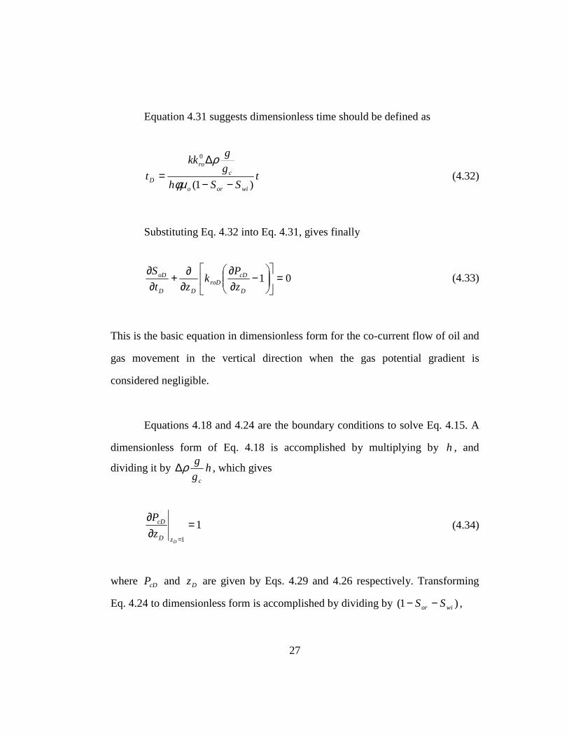
Equation 4.31 suggests dimensionless time should be defined as

tSSh

ggkk

twioro

cro

D )1(

0

−−

∆=

φµ

ρ (4.32)

Substituting Eq. 4.32 into Eq. 4.31, gives finally

01 =

−

∂∂

∂∂+

∂∂

D

cDroD

DD

oD

zP

kzt

S (4.33)

This is the basic equation in dimensionless form for the co-current flow of oil and

gas movement in the vertical direction when the gas potential gradient is

considered negligible.

Equations 4.18 and 4.24 are the boundary conditions to solve Eq. 4.15. A

dimensionless form of Eq. 4.18 is accomplished by multiplying by h , and

dividing it by hgg

c

ρ∆ , which gives

11

=∂∂

=DzD

cD

zP

(4.34)

where cDP and Dz are given by Eqs. 4.29 and 4.26 respectively. Transforming

Eq. 4.24 to dimensionless form is accomplished by dividing by )1( wior SS −− ,

28

wior

wi

zwior

o

SSS

SSS

−−−

=−−

=1

11

0

(4.35)

Subtracting wior

or

SSS

−−1 from both sides of Eq. 4.35,

wior

orwi

zwior

oro

SSSS

SSSS

−−−−

=−−

−

=11

10

(4.36)

Utilizing the definition of dimensionless oil saturation in Eq. 4.28,

1

0=

=DzoDS (4.37)

4.1.2 Oil Flux Equation

Substituting Eq. 4.15 into Eq. 4.5, gives

∆−

∂∂

∂∂=

∂∂

c

cro

o

o

gg

zP

kz

kz

u ρµ

(4.38)

Equation 4.38 can be solved by integration with separation of variables

and applying the upper boundary condition given by Eq. 4.18. The result is

∆−

∂∂

=c

cro

oo g

gzP

kku ρµ

(4.39)

29

Equation 4.39 can be used to determine oil flux at any position and time in the

matrix block.

4.1.2.1 Dimensionless Form of Oil Flux Equation

Multiplying Eq. 4.39 by 0rokh and utilizing the definitions of dimensionless

elevation ( Dz ) from Eq. 4.26 results in

∆−

∂∂

= hgg

zP

kkk

khu

cD

c

ro

ro

oroo ρ

µ 00 (4.40)

Dividing Eq. 4.40 by hgg

c

ρ∆ and utilizing the definitions of

dimensionless capillary pressure and dimensionless oil relative permeability (Eqs.

4.29 and 4.27, respectively),

−

∂∂

=∆

110 D

cDroD

o

cro

o zPkk

ggk

uµρ

(4.41)

This equation suggests

cro

oooD

ggkk

uu

ρ

µ

∆=

0 (4.42)

Substituting this equation into Eq. 4.41,

30

∂∂

−−=D

cDroDoD z

Pku 1 (4.43)

Appendix A shows the development of the finite difference method used

to solve Eqs. 4.33 and 4.43 with the boundary conditions given by Eqs. 4.34 and

4.37 for the top and bottom of the matrix, respectively. The dimensionless

variables Dz , roDk , oDS , cDP , Dt , and oDu are defined by Eqs. 4.26, 4.27, 4.28,

4.29, 4.32, and 4.42, respectively. Appendix G shows the code of the program in

C++. Appendix G also shows the input data listing used by Eclipse to corroborate

the model.

4.2 MODEL VERIFICATION

Table 4.1 shows data for testing Eqs. 4.33 and 4.43. The relative

permeability of oil and capillary pressure were calculated with Corey-type

equations given in Table 4.2 for dimensionless and non-dimensionless saturation

functions. Figures 4.2, 4.3, 4.4, and 4.5 show rok , cP , roDk , and cDP , respectively.

Figure 4.1 shows the model at two different times and also gives the

boundary conditions. The commercial simulator Eclipse was used to verify the

results. Figures 4.6, 4.7, and 4.8 show the formation volume factors for oil, gas

and the solubility of gas in oil ( oB , gB , and sR , respectively) utilized in the

model. A constant gas pressure of 80 atm (Table 4.1) was set at top of the matrix

block. The values utilized for oB , gB , and sR lie in a narrow range close to a

31

pressure value of 80 atm. Figure 4.9 shows the model used with Eclipse utilizing a

gridded system. Table 4.3 shows the geometric information used to construct this

simulation, along with porosity and permeability values. The first and last cells

represent the top and bottom fractures, respectively. In fracture cells capillary

pressure is zero and oil relative permeability and gas relative permeability are

both straight lines of unit slope with respect to their respective saturations.

The model of Fig. 4.9 has a fracture cell at the top and a fracture cell at the

bottom. Intermediate cells are matrix. In the top cell a well is connected and

controlled by constant injection pressure equal to 80 atm to simulate pressure

maintenance. The bottom cell has another well connected to the cell. This well is

controlled by constant pressure equal to 80.03 atm, which is the value based on

the gas gradient in the fracture.

Figure 4.10 shows saturation profiles obtained with the vertical drainage

model (Eq. 4.33) vs. Eclipse results. This graph shows that saturation profiles

match better at later run times. At very early times there is not a good match in the

saturation profiles. This mismatch affects oil flux from 100 to 1500 days

approximately (Fig. 4.11). Figure 4.10 also shows that at infinite time, the

saturation profile matches the saturation given by the static capillary pressure

profile. From this, there are two observations. First, capillarity retains oil in the

matrix. The greater the capillarity at high oil saturations, the greater the residual

32

oil saturation. Second, there is a limit in oil saturation given by the capillary

pressure curve at static conditions.

Figure 4.11 shows oil flux for Eq. 4.43 vs. Eclipse results. Figure 4.12

shows the cumulative oil production for both Eq. 4.43 and Eclipse. The difference

is due to neglecting gas viscous pressure drop in Eq. 4.33. Oil flux from Eclipse

(Fig. 4.11) shows there is a mismatch between 100 and 1500 days due to effect of

neglecting gas viscous pressure drop. Appendix F discusses this result compared

with that obtained from using gas relative permeability of unitary slope with

respect to gas saturation, which gives a better match. Additionally in Fig. 4.11, at

approximately 2600 days there is a small “peak” in Eclipse results, which is a

numerical error. Dividing only the bottom cell in 20 sub-cells partially smoothed

the “peak”. Figure 4.13 shows results of grid refinement to overcome this

numerical error sub-gridding only the bottom cell. The grid in Fig. 4.11 is 1x1x20

for x, y, and z directions.

4.2.1 Capillary Minimum Oil Saturation

There is a maximum capillary pressure defined at a minimum oil

saturation ( minoS ), which corresponds to the maximum capillary pressure

allowable with gravity segregation at the block matrix height ( h ). This maximum

of dimensionless capillary pressure corresponds to

1=cDP (4.44)

33

In the unusual case of threshold capillary pressure being greater than this

value, it is not possible to get any oil from the matrix. To get minoS we utilize the

dimensionless capillary pressure form given in Table 4.2:

( ) pceoDcDcD SPP −= 10 (4.45)

Substituting Eq. 4.44 in Eq. 4.45,

pce

cDoD P

S

1

0min11

−= (4.46)

minoDS is obtained substituting pce and 0cDP from Table 4.2 into Eq. 4.46

and from the definition of dimensionless oil saturation (Eq. 4.28) we get minoS . cP

evaluated at minoS and minoS are given in Table 4.4.

4.3 GRAVITY DRAINAGE WITH NEGLIGIBLE CAPILLARY PRESSURE

Equation 4.33 includes viscous, capillary, and gravity forces. To simplify

its analysis in this section capillary forces are considered negligible. From Eq.

4.13 considering 0=cP ,

c

go

gg

zzρ∆+

∂Φ∂

=∂Φ∂

(4.47)

34

Introducing the consideration given by Eq. 4.9

≈

∂Φ∂

0z

g ,

c

o

gg

zρ∆=

∂Φ∂

(4.48)

Substituting Eq. 4.48 in the Darcy’s law (Eq. 4.1),

co

roo g

gkku ρ

µ∆−= (4.49)

Substituting Eq. 4.49 into the continuity equation (Eq. 4.5) gives

0=

∆

∂∂−

∂∂

co

roo

ggk

kzt

S ρµ

φ (4.50)

considering k , oµ , and ρ∆ constant,

0=∂

∂∆−

∂∂

zk

ggk

tS ro

co

o ρµ

φ (4.51)

This is a non-linear first-order partial differential equation. Equation 4.51

can also be obtained from Eq. 4.15 considering 0=∂∂

zPc . Multiplying Eq. 4.51 by

0/ rokh ,

35

00 =∂

∂∆−

∂∂

D

roD

co

o

ro zk

ggk

tS

kh ρ

µφ (4.52)

where Dz is defined with Eq. 4.26 and roDk is defined with Eq. 4.27. Multiplying

Eq. 4.52 by wior

wior

SSSS

−−−−

11

,

( )

01

0=

∂∂

−∂

∂

∆

−−

D

roDoD

cro

wioro

zk

tS

ggkk

SSh

ρ

φµ (4.53)

oDS is defined with Eq. 4.28. Substituting Eq. 4.32 for Dt in Eq. 4.53,

0=∂

∂−

∂∂

D

roD

D

oD

zk

tS

(4.54)

or

0=∂∂

−∂∂

D

oD

oD

roD

D

oD

zS

dSdk

tS

(4.55)

This is a form of the “Buckley-Leverett” equation, but with a negative

sign instead of a positive one because of the sign convention with respect to

depth.

36

Equation 4.49 (oil flux equation) in dimensionless form is obtained by

dividing by 0rok ,

croD

oro

o

ggkk

ku ρ

µ∆−=0 (4.56)

where roDk is given by Eq. 4.27 and considering the definition of oDu given by

Eq. 4.42,

roDoD ku −= (4.57)

This means that dimensionless oil flux at any point in the matrix is equal

to dimensionless relative permeability of oil for the case of no capillarity, as

expected the solution of Eq. 4.55 by the method of characteristics is

DSoD

roDSD t

dSdkz

oD

oD−=1 (4.58)

At the bottom of the matrix, 0=Dz , thus

oD

oD

SoD

roDSD

dSdk

t 1= (4.59)

37

Dimensionless oil flux from matrix to fracture can also be represented as a

dimensionless transfer function from matrix to fracture. Appendix B shows the

definitions of dimensionless variables when utilizing transfer function instead of

the flux equation. From Eq. 4.43 and Eq. B.8,

oDoD u=τ (4.60)

Where oDτ is defined with Eq. B.7 from Appendix B. To test the model

with no capillarity, dimensionless relative permeability of oil in Table 4.2 was

utilized.

The velocity of a given saturation is proportional to the derivative of oil

relative permeability. Figure 4.14b shows the results of the calculations related to

dimensionless oil relative permeability (Fig. 4.14a). Figure 4.15a shows

dimensionless oil relative permeability at the outlet of the matrix. From Eq. 4.57,

the dimensionless relative permeability of oil is the oil flux (Eq. 4.57) and the

dimensionless time for that oil flux is calculated with the inverse of the derivative

of dimensionless oil relative permeability (Eq. 4.59).

Due to Fig. 4.15a shows roDk at the outlet of the matrix block then this

roDk is the oil flux at the outlet of the matrix block accordingly to Eq. 4.57.

Declination of oil flux starts at dimensionless time equal )1(

1' =oDSkroD

, then oil

38

flux has a unitary value in dimensionless time from zero to )1(

1' =oDSkroD

and

after that oil flux decreases accordingly to '

1

roDk

. Figure 4.16 shows saturation

profiles at different times for the analytical saturation profiles compared with the

finite difference solution. The mismatch between analytical and numerical

profiles is probably due to numerical dispersion.

Figure 4.17 shows the transfer function for the analytical and the finite

difference methods. This figure also shows the time of declining oil flux from the

matrix, which depends on the slope of the oil relative permeability curve. When

we have a unit slope in the oil relative permeability (the ideal case of free oil

flow) the initiation of flux declining is at 1=Dt . The flux decline curve depends

on the shape of the oil relative permeability. The more concave up the rok curve

the steeper the decline in oil flux.

From Fig. 4.17, there are two types of flow from matrix to fracture with no

capillary pressure. Both flows converge at the following dimensionless time:

)1(1

' ==

oDroDD Sk

t (4.61)

For )1(

1' =

≤oDroD

D Skt ,

39

1=oDτ (4.62)

For )1(

1' =

≥oDroD

D Skt dimensionless oil flux (or transfer function) is

given by Eq. 4.57, therefore from Eq. 4.60,

roDoD k=τ (4.63)

Substituting the derivative of roDk into Eq. 4.59, where 0=Dz ,

oooD eoDo

oDe

oDoSD Se

SSe

t == −1

1 (4.64)

Substituting Eq. 4.63 in Eq. 4.64 and considering oeoDroD Sk = ,

oDo

oD

roDo

oDSD e

Ske

St

oD τ== (4.65)

This equation relates dimensionless oil saturation at the outlet of the

matrix with dimensionless transfer function also at the outlet of the matrix and

dimensionless time.

To get average oil saturation at time Dt with no capillary pressure, is by

integrating the curve for a specific Dt (Fig. 4.14b). For )1(

1' =

≤oDroD

D Skt and

substituting the derivative of oil relative permeability definition in Eq. 4.58,

40

De

oDoSD tSez o

oD

11 −−= (4.66)

Average oil saturation is obtained by integrating Eq. 4.66 from zero to one

and dividing by Dz ,

( )∫ −−=1

0

1 ~~11oDD

eoDo

DoD SdtSe

zS o (4.67)

where oDS is the average dimensionless oil saturation and oDS~ is an integration

variable. Solving Eq. 4.67 and considering 1=Dz ,

DoD tS −=1 (4.68)

This is the average oil saturation for ( )11

' =≤

oDroDD Sk

t . To get an average

oil saturation for )1(

1' =

≥oDroD

D Skt (Fig. 4.14b) is with the integration process,

but changing Eq. 4.66 as a function of Dz ,

11

1 −

−=

oe

Do

DoD te

zS (4.69)

integrating from zero to one and dividing by Dz ,

41

D

e

Do

D

DoD zd

tez

hS

o ~~11 11

1

0

−

∫

−= (4.70)

where Dz~ is an integration variable. Solving Eq 4.70 and considering 1=Dh ,

( )111

−

−=

o

o

ee

DoDooD

teteS (4.71)

that is the average dimensionless oil saturation for )1(

1' =

≥oDroD

D Skt .

To obtain the transfer function as a function of average oil saturation for

( )11

' =≥

oDroDD Sk

t , first obtain oDoD S/τ from Eq. 4.65,

DozoD

oD

teSD

1

1

==

τ (4.72)

Substituting Eq. 4.72 into Eq. 4.71,

( )1

1−

−=

o

o

ee

oD

oD

Do

oDooD

SeS

eSτ

τ (4.73)

Substituting Eq. 4.63 into Eq. 4.73 and considering that oeoDroD Sk = ,

42

( )1

1−

−=

o

oo

o

ee

oD

eoD

eoDo

oDooD

SS

SeS

eS (4.74)

or

oDo

ooD S

ee

S1−

= (4.75)

This equation suggests the calculation of average oil saturation in the

matrix for ( )11

' =≥

oDroDD Sk

t . Substituting oDS from Eq. 4.75 into Eq. 4.73,

( ) 11 −

−=

o

o

ee

oDo

ooDoD Se

eττ (4.76)

Considering that oeoDroDoD Sk ==τ in the right hand side of Eq. 4.76 and

substituting Eq. 4.75 into Eq. 4.76,

( )1

11

−

−

−=

o

oo e

e

oDo

o

e

o

oDo

oD Se

ee

Se

τ (4.77)

or

43

oe

o

oDooD e

Se

−=

1τ (4.78)

or from Eq. 4.63,

oe

o

oDoroD e

Sek

−=

1 (4.79)

Due to the fact that dimensionless transfer function with gravity drainage

and no capillary pressure is equal to dimensionless oil relative permeability (Eq.

4.63), roDk from Eq. 4.79 can be a pseudo oil relative permeability ( *roDk ) with no

capillarity to apply in a dual porosity model.

oe

o

oDoroD e

Sek

−=

1* (4.80)

this is for )1(

1' =

≥oDroD

D Skt . For

)1(1

' =≤

oDroDD Sk

t pseudo relative permeability

of oil is

1* =roDk (4.81)

Figure. 4.18 shows average oil saturation calculated with Eqs. 4.68 and

4.71, with the average oil saturation calculated from the vertical drainage model.

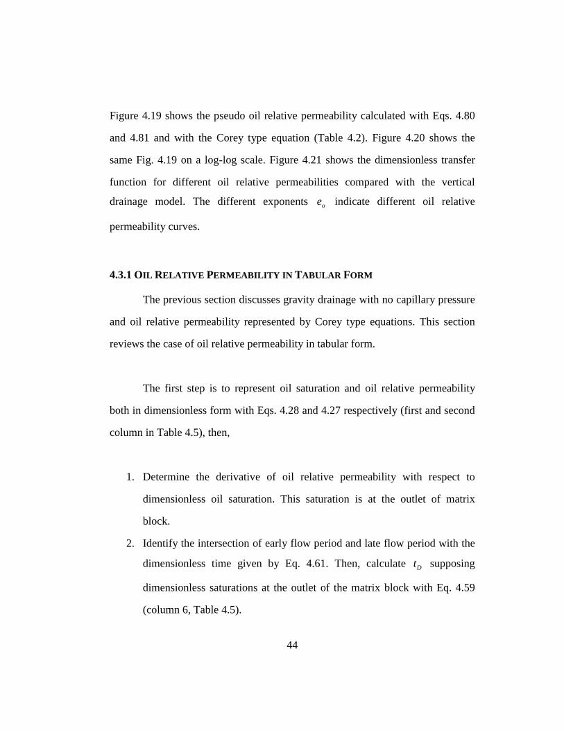
44

Figure 4.19 shows the pseudo oil relative permeability calculated with Eqs. 4.80

and 4.81 and with the Corey type equation (Table 4.2). Figure 4.20 shows the

same Fig. 4.19 on a log-log scale. Figure 4.21 shows the dimensionless transfer

function for different oil relative permeabilities compared with the vertical

drainage model. The different exponents oe indicate different oil relative

permeability curves.

4.3.1 OIL RELATIVE PERMEABILITY IN TABULAR FORM

The previous section discusses gravity drainage with no capillary pressure

and oil relative permeability represented by Corey type equations. This section

reviews the case of oil relative permeability in tabular form.

The first step is to represent oil saturation and oil relative permeability

both in dimensionless form with Eqs. 4.28 and 4.27 respectively (first and second

column in Table 4.5), then,

1. Determine the derivative of oil relative permeability with respect to

dimensionless oil saturation. This saturation is at the outlet of matrix

block.

2. Identify the intersection of early flow period and late flow period with the

dimensionless time given by Eq. 4.61. Then, calculate Dt supposing

dimensionless saturations at the outlet of the matrix block with Eq. 4.59

(column 6, Table 4.5).

45

3. Determine average oil saturation ( oDS ) in the matrix block for each Dt

related to oil saturation at the outlet of the matrix. For Dt less or equal

than Dt from Eq. 4.61, oDS is calculated with Eq. 4.68. For Dt greater or

equal than Dt from Eq. 4.61, construct a saturation profile in the matrix

( oDS vs. matrix height) with Eq. 4.58, the area bellow the curve (integral)

is the average oil saturation (Fig. 4.14 b).

4. Determine a constant eC for each data in the table with Eq. 4.82. In this

case eC is the same for each saturation value (column 8, Table 4.5). From

Eq. 4.76.

oD

oDe

SS

C−

=1

1 (4.82)

5. Determine pseudo dimensionless oil relative permeability ( *roDk ) with Eq.

4.80 and Eq. 4.81 substituting the value of eC instead of oe . Finally,

obtain pseudo oil relative permeability substituting *roDk instead of roDk

into Eq. 4.27.

The previous sections consider gravity effects with no capillary pressure.

Figure 4.22 shows the effects in the transfer function with variation of capillary

pressure, utilizing different capillary exponents ( pce ). In general, the greater the

exponent the less the capillary effect. When capillary pressure increases the

transfer function declines more quickly.

46

The next chapter reviews dual porosity models that include gravity and

capillary pressure effects. Then we will talk more about capillarity in the next

chapter.

In summary, this chapter reviews an equation for gravity drainage of oil

and gas, which was solved with the finite difference method and gives acceptable

results comparing with results obtained from the Eclipse numerical simulator.

Additionally, neglecting capillary pressure in the non-linear partial differential

equation an analytical solution is obtained that is function of the derivative of oil

relative permeability. From this, a pseudo oil relative permeability to be used in

dual porosity models is analytically obtained from a Corey type representation of

oil relative permeability. Finally, a procedure was established to obtain a pseudo

oil relative permeability with tabular data of oil relative permeability.

47

Table 4.1: Basic data used for gravity segregation model.

Table 4.2: Saturation functions used in calculations (dimensionless and non-dimensionless).

ge

wior

ororgrg SS

SSkk

−−

−−=1

10 32.00 =rgk 2=ge

oe

wior

orororo SS

SSkk

−−

−=1

0 10 =rok 3=oe

pce

wior

orocc SS

SSPP

−−

−−=1

10 60 =cP atm 6=pce

eooDroDroD Skk 0= 10 =roDk 3=oe

( ) oeoDcDcD SPP −= 10 19.290 =cDP

6=pce

Description ValueResidual total liquid saturation 0.55Residual oil saturation 0.40Initial (residual) water saturation 0.15Oil density, g/cm 3 0.814242Gas density, g/cm 3 0.106556End-point oil relative permeability 1.00End-point gas relative permeability 0.32Maximum gas saturation 0.45Maximum oil saturation 0.85Critical gas saturation 0.00Matrix block thickness, m 3.00Oil viscosity, cp 3.14Gas viscosity, cp 0.0149Matrix porosity 0.06Matrix permeability, md 0.20Presssure at top of matrix, atm 80

48

Table 4.3: Geometry, porosity, and permeability utilized in Eclipse for a matrix block model with top and bottom fractures.

Table 4.4: Minimum saturation with its capillary pressure (dimensionless and non-dimensionless) for a matrix block of 3 m thickness.

Parameter Value 0

cDP 29.19 0rDk 1.0

minoDS 0.4301

minoS 0.5935

( )minoDcD SP 1.0

( )minoc SP 0.2055

Cells in z Direction1 2 to 21 22

∆X, cm 15 15 15∆Y, cm 15 15 15∆Z, cm 0.1 15 0.1Porosity, fraction 1 0.06 1k- x direction, darcy 5 0.2 5k- y direction, darcy 5 0.2 5k- z direction, darcy 5 0.2 5Tops, m 1200*

*top of cell 2 only (matrix begins)

Description

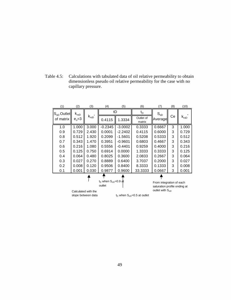
49

Table 4.5: Calculations with tabulated data of oil relative permeability to obtain dimensionless pseudo oil relative permeability for the case with no capillary pressure.

(1) (2) (3) (4) (5) (6) (7) (8) (10)

tD

0.4115 1.3334 Outlet of matrix

1.0 1.000 3.000 -0.2345 -3.0002 0.3333 0.6667 3 1.0000.9 0.729 2.430 0.0001 -2.2402 0.4115 0.6000 3 0.7290.8 0.512 1.920 0.2099 -1.5601 0.5208 0.5333 3 0.5120.7 0.343 1.470 0.3951 -0.9601 0.6803 0.4667 3 0.3430.6 0.216 1.080 0.5556 -0.4401 0.9259 0.4000 3 0.2160.5 0.125 0.750 0.6914 0.0000 1.3333 0.3333 3 0.1250.4 0.064 0.480 0.8025 0.3600 2.0833 0.2667 3 0.0640.3 0.027 0.270 0.8889 0.6400 3.7037 0.2000 3 0.0270.2 0.008 0.120 0.9506 0.8400 8.3333 0.1333 3 0.0080.1 0.001 0.030 0.9877 0.9600 33.3333 0.0667 3 0.001

Calculated with the slope between data

tD when SoD=0.9 at outlet

tD when SoD=0.5 at outlet

kroD*SoD

AverageCe

From integration of each saturation profile ending at outlet with SoD

kroD'kroD

eo=3

tDSoD Outlet of matrix

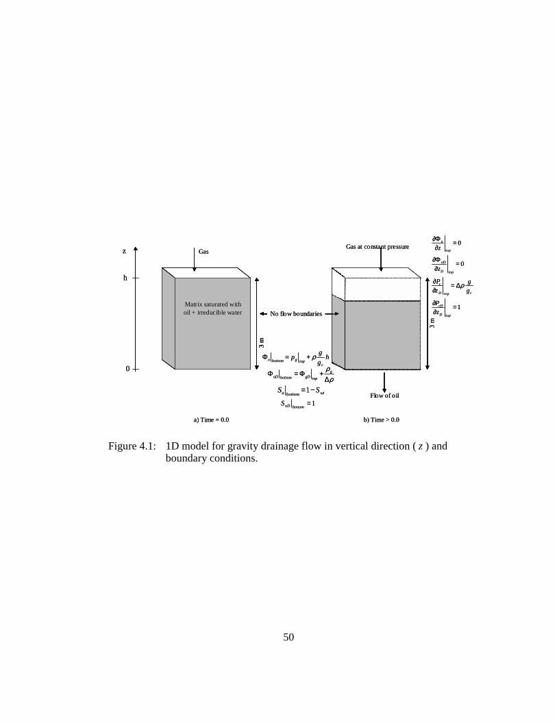
50

Figure 4.1: 1D model for gravity drainage flow in vertical direction ( z ) and boundary conditions.

Matrix

b) Time > 0.0

3 m

a) Time = 0.0

GasGas at constant pressure

No flow boundariesMatrix saturated with oil + irreducible water

3 m

Flow of oil

1

0

0

=∂∂

∆=∂∂

=∂Φ∂

=∂Φ∂

topD

cD

ctopD

c

topD

oD

top

o

zP

gg

zP

z

z

ρ

hggp

ctopgbottomo ρ+=Φ

ρρ∆

+Φ=Φ g

topgDbottomoD

wibottomo SS −=1

1=bottomoDS

0

h

z

Matrix

b) Time > 0.0

3 m

a) Time = 0.0

GasGas at constant pressure

No flow boundariesMatrix saturated with oil + irreducible water

3 m

Matrix saturated with oil + irreducible water

3 m

Flow of oil

1

0

0

=∂∂

∆=∂∂

=∂Φ∂

=∂Φ∂

topD

cD

ctopD

c

topD

oD

top

o

zP

gg

zP

z

z

ρ

hggp

ctopgbottomo ρ+=Φ

ρρ∆

+Φ=Φ g

topgDbottomoD

wibottomo SS −=1

1=bottomoDS

0

h

z

51

Figure 4.2: Relative permeability of oil utilized for simulation of gravity drainage in a matrix-block.

Figure 4.3: Gas-oil capillary pressure utilized for simulation of gravity drainage in a matrix block with top and bottom fractures.

0.0

0.2

0.4

0.6

0.8

1.0

0.3 0.4 0.5 0.6 0.7 0.8 0.9Oil Saturation

Oil

Rel

ativ

e P

erm

eabi

lity

0

1

2

3

4

5

6

0.4 0.5 0.6 0.7 0.8 0.9Oil Saturation

Cap

illary

Pre

ssur

e, a

tm

52

Figure 4.4: Dimensionless oil relative permeability utilized for simulation of gravity drainage in a matrix block with top and bottom fractures.

Figure 4.5: Dimensionless gas-oil capillary pressure for simulation of gravity drainage in a matrix block with top and bottom fractures.

0.0

0.2

0.4

0.6

0.8

1.0

0.0 0.2 0.4 0.6 0.8 1.0Dimensionless Oil Saturation

Dim

ensi

onle

ss O

il R

elat

ive

Perm

eabi

lity

0

5

10

15

20

25

30

0.0 0.2 0.4 0.6 0.8 1.0Dimensionless Oil Saturation

Dim

ensi

onle

ss C

apill

ary

Pre

ssur

e

53

Figure 4.6: Oil formation volume factor utilized in simulation of gravity drainage in a matrix block with top and bottom fractures.

Figure 4.7: Gas formation volume factor utilized in simulation of gravity drainage in a matrix block with top and bottom fractures.

1.12

1.16

1.20

1.24

1.28

1.32

1.36

0 50 100 150 200 250Pressure, atm

Oil

Form

atio

n Vo

lum

e Fa

ctor

, cm

3 /std

.cm

3

0.00

0.01

0.02

0.03

0.04

0.05

0.06

0.07

0.08

0.09

0 20 40 60 80 100 120 140Pressure, atm

Gas

form

atio

n vo

lum

e fa

ctor

, cm

3 /std

.cm

3

54

Figure 4.8: Solubility of gas in oil utilized for simulation of gravity drainage in a matrix block with top and bottom fractures.

Figure 4.9: 1D simulation with Eclipse to simulate gravity drainage in a matrix block with top and bottom fractures.

0

20

40

60

80

100

120

140

160

10 20 30 40 50 60 70 80 90Pressure, atm

Solu

bilit

y of

Gas

in O

il, s

td.c

m3 /s

td.c

m3

Matrix saturated with oil + irreducible water

k=0.2 md

3 m

Gas at constant pressure

Oil Production in bottom cell

0.1 cm, k=5 Darcy

0.1 cm, k=5 Darcy

Top cell

Bottom cell

Matrix saturated with oil + irreducible water

k=0.2 md

3 m

Gas at constant pressure

Oil Production in bottom cell

0.1 cm, k=5 Darcy

0.1 cm, k=5 Darcy

Top cell

Bottom cell

55

Figure 4.10: Oil saturation profiles in the matrix block with gravity drainage, simulating with the vertical drainage equation and Eclipse.

Figure 4.11: Oil flux from the vertical drainage equation and Eclipse simulating a matrix block with gravity drainage.

0

50

100

150

200

250

300

0.5 0.6 0.7 0.8 0.9 Oil Saturation

Hei

ght A

bove

Mat

rix B

otto

m, c

m

Eclipse 736 days

Eclipse 1092 days

Eclipse 2557 days

Vertical drainage equation 729 days

Vertical drainage equation 1094 days

Vertical drainage equation 2553 days

Static

1E-08

1E-07

1E-06

1E-05

1E-04

10 100 1000 10000Time, days

Oil

Flux

, bbl

/day

/ft2

Vertical drainage equation

Eclipse

56

Figure 4.12: Cumulative oil production from a matrix block with top and bottom fractures simulating gravity drainage with vertical drainage equation and Eclipse.

Figure 4.13: Oil flux for the times having numerical errors. Refinement is only in the bottom cell with 10 and 20 sub-cells for gravity drainage case.

0

0.001

0.002

0.003

0.004

0.005

0.006

0 1000 2000 3000 4000 5000 6000 7000

Time, days

Cum

ulat

ive

Oil

Prod

uctio

n, b

bl

Vertical drainage equation

Eclipse

1E -06

1E -05

1E -04

1000 100 00T im e , days

Oil

Flux

, bbl

/d/ft

2

N o rm a l g rid , 1 X1X2 2 ce lls (x,y, a nd z)

O n ly b o tto m ce ll re fine d w ith 10 sub -ce lls in z

O n ly b o tto m ce ll re fine d w ith 20 sub -ce lls in z

57

a) Dimensionless oil relative permeability.

b) Saturation profiles at different dimensionless time.

Figure 4.14: Dimensionless oil saturation profiles at different dimensionless times and the relation with dimensionless oil relative permeability for the analytical solution of gravity drainage with no capillary pressure in a matrix block.

0.0

0.2

0.4

0.6

0.8

1.0

0 0.2 0.4 0.6 0.8 1

Dimensionless Oil Saturation

Dim

ensi

onle

ss O

il R

elat

ive

Per

mea

bilit

y

0.0

0.2

0.4

0.6

0.8

1.0

0 0.2 0.4 0.6 0.8 1

Dimensionless Oil Saturation

Dim

ensi

onle

ss M

atrix

Hei

ght

tD

0.1

0.2

0.3

0.4

0.5

58

a) Dimensionless oil relative permeability at the outlet of the matrix vs. dimensionless time.

b) Diagram dimensionless matrix height vs. dimensionless time.

Figure 4.15: Dimensionless oil relative permeability at the outlet of the matrix and diagram dimensionless matrix height vs. dimensionless time for gas oil gravity drainage with no capillary pressure.

0.0

0.2

0.4

0.6

0.8

1.0

0 0.5 1 1.5 2 2.5 3Dimensionless Time

Dim

ensi

onle

ss M

atrix

Hei

ght

0

0.2

0.4

0.6

0.8

1

0 0.5 1 1.5 2 2.5 3

Dimensionless Time

Dim

ensi

onle

ss O

il R

elat

ive

Per

mea

bilit

y

59

Figure 4.16: Saturation profiles at different times for gravity drainage in a matrix block with no capillarity for vertical drainage equation and analytical solution.

Figure 4.17: Dimensionless transfer function for gas oil gravity drainage in a matrix block with no capillarity obtained with the analytical solution and the vertical drainage equation.

0

100

200

300

0.4 0.5 0.6 0.7 0.8Oil Saturation

Mat

rix H

eigh

t, cm

429.1 days (Analytical)

644 days (Analytical)

1073 days (Analytical)

429.1 days (Vertical drainage equation)

644 days (Vertical drainage equation)

1073 days (Vertical drainage equation)

0.01

0.10

1.00

0.010 0.100 1.000 10.000Dimensionless Time

Dim

ensi

onle

ss T

rans

fer F

unct

ion

Analytical solution

Vertical drainage equation

60

Figure 4.18: Dimensionless average oil saturation vs. time obtained from gas-oil gravity drainage for a matrix block with vertical drainage equation with no capillarity and the analytical solution also with no capillarity.

Figure 4.19: Pseudo oil relative permeability obtained for gravity drainage and no capillary pressure and Corey type oil relative permeability ( 3=oe ).

0.0

0.2

0.4

0.6

0.8

1.0

0.0 0.5 1.0 1.5 2.0 2.5 3.0 3.5 4.0

Dimensionless Time

Dim

ensi

onle

ss A

vera

ge O

il Sa

tura

tion

Vertical drainage equation with no capillarypressure

Analytical solution with no capillary pressure

0.0

0.2

0.4

0.6

0.8

1.0

0.0 0.1 0.2 0.3 0.4 0.5 0.6 0.7 0.8 0.9 1.0Dimensionless Average Oil Saturation

Dim

ensi

onle

ss O

il R

elat

ive

Per

mea

bilty

Pseudo dimensionless oil relativepermeability (kroD*)

True dimensionless oil relativepermeability with eo=3

61

Figure 4.20: Pseudo oil relative permeability obtained for gravity drainage and no capillary pressure and Corey type oil relative permeability ( 3=oe ).

Figure 4.21: Dimensionless transfer function for different dimensionless oil relative permeabilities (different oe ) obtained with analytical solution and vertical drainage equation.

0.0

0.1

1.0

0.1 1.0Dimensionless Average Oil Saturation

Dim

ensi

onle

ss P

seud

o O

il R

elat

ive

Perm

eabi

lity

Pseudo dimensionless oil relativepermeability (kroD*)

True dimensionless oil relativepermeability with eo=3

0.01

0.1

1

0.01 0.1 1 10Dimensionless Time

Dim

ensi

onle

ss T

rans

fer F

unct

ion

Analytical Solution (eo=2)

Analytical solution (eo=5)

Vertical drainage equation (eo=2)

Vertical drainage equation (eo=5)

62

Figure 4.22: Dimensionless transfer function for gravity drainage in a matrix block with and without capillarity ( pce ) simulated with the vertical drainage equation neglecting gas viscous pressure drop.

0.01

0.10

1.00

0.01 0.10 1.00 10.00DimensionlessTime

Dim

ensi

onle

ss T

rans

fer F

unct

ion

With no capillary pressure

With capillarity and capillary exponent epc=6

With capillarity and capillary exponent epc=2

63

Chapter 5 Dual Porosity Gravity Segregation Models

This chapter reviews different dual porosity transfer function models for

gravity drainage including capillary and gravity forces. Additionally, this chapter

presents a procedure to obtain pseudo capillary pressure curve to be used in dual

porosity models using fine grid simulation in a matrix block, or an exponential

equation at late flow with gravity drainage.

5.1 GRAVITY DRAINAGE FLUX CALCULATION

Equation 4.32 represents the oil flux at any vertical position in a matrix

block. To evaluate the flux out of the matrix with gravity drainage, Eq. 4.32 must

be evaluated at the bottom boundary of the matrix. Observing Eq. 4.32, the flux

from matrix to fracture with gravity drainage includes relative permeability to oil,

capillary pressure and a gravity term.

On the other hand, dual porosity models utilize average properties for the

entire matrix block and the entire surrounding fracture system. Some models have

the capacity to calculate an effective level of fluids in the simulation cell to

compute transfer due to gravity. Section 4.4 of the previous chapter evaluates

properties with average saturation and no capillarity. This chapter presents

various dual porosity models for matrix-fracture transfer that include the effects

of viscous flow, gravity, and capillarity.

64

5.2 ECLIPSE MODEL

Based on positive flow being out of the matrix, the basic Eclipse dual

porosity gravity drainage model considers the following equations for oil and gas

flow. This is the standard model in most dual porosity simulators.

( )

∆−∆+−=

cgmDgfDofomromo g

gSSzppk ρσλτ2

(5.1)

and

( )

∆−∆−−+−=

cgmDgfDcfcmofomrgmg g

gSSzPPppk ρσλτ2

(5.2)

where

ρ∆ = go ρρ − , 3/ cmgm

λ = mobility, cpcmcmstd //. 33

z∆ = matrix block height, cm

gfDS = fractional volume of movable gas phase in the fracture

gmDS = fractional volume of movable gas phase in the matrix

Subscripts o , g , f , m , and r refer to oil, gas, fracture, matrix, and

relative, respectively.

65

Since pressure is calculated at the center of the simulation cell, the gravity

term is calculated with half the height of the matrix block. Note that gravity

affects the oil equation opposite to the gas equation.

Figure 5.1 shows a schematic of the Eclipse model. The fractional volume

of moveable gas (Appendix C) in the matrix is calculated as

wio

gmgmD SS

SS

−−=

min1 (5.3)

where,

gmS = gas saturation in the matrix

minoS = minimum oil saturation in the matrix

There is a similar saturation equation for the fracture ( )gfDS . For the

purpose of the present study initial gas saturation is zero. In Eqs. 5.1 and 5.2, roλ

and rgλ are the oil and gas mobilities, respectively:

oo

roro B

kµ

λ = (5.4)

gg

rgrg B

kµ

λ = (5.5)

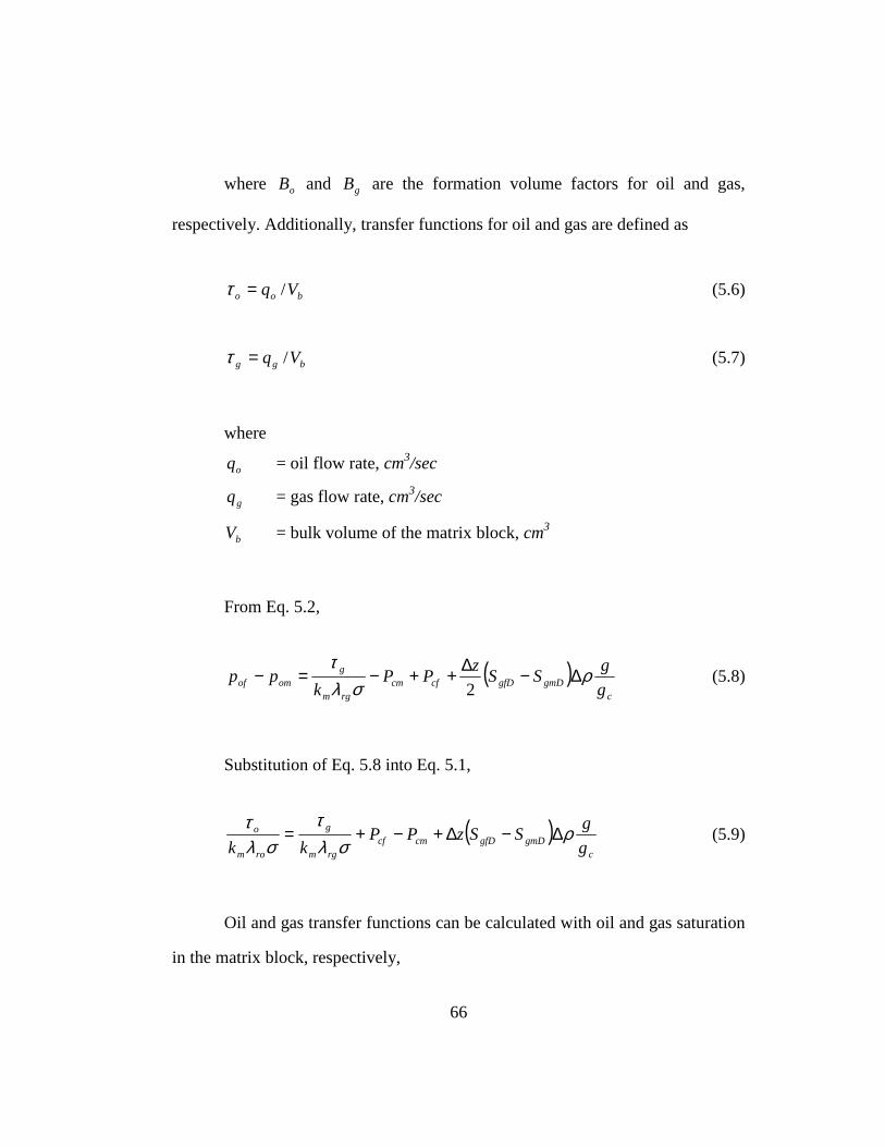
66

where oB and gB are the formation volume factors for oil and gas,

respectively. Additionally, transfer functions for oil and gas are defined as

boo Vq /=τ (5.6)

bgg Vq /=τ (5.7)

where

oq = oil flow rate, cm3/sec

gq = gas flow rate, cm3/sec

bV = bulk volume of the matrix block, cm3

From Eq. 5.2,

( )c

gmDgfDcfcmrgm

gomof g

gSSzPPk

pp ρσλ

τ∆−∆++−=−

2 (5.8)

Substitution of Eq. 5.8 into Eq. 5.1,

( )c

gmDgfDcmcfrgm

g

rom

o

ggSSzPP

kkρ

σλτ

σλτ

∆−∆+−+= (5.9)

Oil and gas transfer functions can be calculated with oil and gas saturation

in the matrix block, respectively,

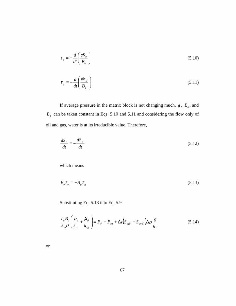
67

−=

o

oo B

Sdtd φτ (5.10)

−=

g

gg B

Sdtd φ

τ (5.11)

If average pressure in the matrix block is not changing much, φ , oB , and

gB can be taken constant in Eqs. 5.10 and 5.11 and considering the flow only of

oil and gas, water is at its irreducible value. Therefore,

dtdS

dtdS go −= (5.12)

which means

ggoo BB ττ −= (5.13)

Substituting Eq. 5.13 into Eq. 5.9

( )c

gmDgfDcmcfrg

g

ro

o

m

oo

ggSSzPP

kkkB ρ

µµσ

τ∆−∆+−=

+ (5.14)

or

68

( )

∆−∆+−

+

=c

gmDgfDcmcf

rg

g

ro

oo

mo g

gSSzPP

kkB

k ρµµ

στ (5.15)

The gas viscosity value is usually very small compared with that of oil.

Therefore, the second term in parentheses in the denominator of Eq. 5.15 can be

considered negligible, and

( )

∆−∆−−−=

cgmDgfDcfcmromo g

gSSzPPk ρσλτ (5.16)

If the fracture is completely filled with gas (Fig. 5.1), 1=gfDS , therefore

( )

∆−∆−−−=

cgmDcfcmromo g

gSzPPk ρσλτ 1 (5.17)

Additionally, omDgmD SS =−1 . Substituting into Eq. 5.10, and considering

that gmDomD SS −=1 ,

∆∆−−=

coDcfcm

romo

ggzSPP

kdt

dS ρφ

σλ (5.18)

Separating variables and integrating,

69

( )

∫

∆∆−−

=tS

S

coDcfcmro

o

m

oo

oi

ggzSPPk

dSk

tρ

σφµ

(5.19)

Appendix D shows Eqs. 5.17 and 5.19 in dimensionless form. To test the

model, we use the information given in Table 4.1. Dimensionless oil relative

permeability and capillary pressure both consider variations from zero to one as

shown in Figs. 4.4 and 4.5. Table 4.2 shows these equations.

The exponents 6=pce and 3=oe were utilized for dimensionless relative

permeability for oil and dimensionless capillary pressure. Additionally, 10 =roDk

and 10 =cDP were used. Dimensionless oil saturation (Appendix S) is defined as:

wio

oooD SS

SSS

−−−

=min

min

1 (5.20)

minoS is the minimum oil saturation obtained from capillary pressure at

static conditions at the top of the matrix block. To compare results obtained with

Eqs. 5.17 and 5.19, the dual porosity option was utilized with the Eclipse

simulator (Eclipse Technical Description, 1982-2000). Figure 5.2 shows the

model utilized by Eclipse, which consists of two matrix blocks and two fracture

blocks. Each matrix block is connected to its corresponding fracture block and

both fracture blocks are interconnected. During the runs, the bottom matrix block

was inactive to observe the transfer function from the upper matrix block to

70

fractures. The pore volume of fracture blocks was greater than that of the upper

matrix block in order to have no flow restrictions from matrix to fracture.

Table 5.1 gives the information utilized for the Eclipse runs. The porosity

for matrix corresponds to a field case (rock dolomite) and porosity in fracture

usually is given 10% of the total matrix-fracture bulk volume, but in this case was

considered equal to 6%. Figures 4.6, 4.7, and 4.8 show the formation volume

factors and solubility of gas in oil, respectively, that are used in the simulation.

The integral Eq. 5.19 is a function of oil relative permeability and

capillary pressure, which are functions of saturation. To solve Eq. 5.19, the

analytical equations for rok and cP from Table 4.2 were substituted into Eq. 5.19

and solved numerically from oiS to the oil saturation of interest. Figure 5.3 shows

the results of oil saturation vs. time obtained from integration. This figure also

shows results from the Eclipse simulator. Additionally, the transfer functions

calculated with both Eq. 5.17 and the Eclipse simulator are given in Fig. 5.4.

5.3 QUANDALLE AND SABATHIER MODEL

Figure 5.5 illustrates the matrix-fracture transfer model utilized by

Quandalle and Sabathier (1989). For the purpose of this study we utilize only the

flow in the vertical direction. The flow of oil from the matrix-fracture cell to the +z face (Fig. 5.5) is given by

71

( )2/zyxkq omofzromoz ∆

∆∆Φ−Φ−= ++ λ (5.21)

where

Φ = phase potential, atm

x∆ = dimension of the matrix-fracture block in the x direction,

cm

y∆ = dimension of the matrix-fracture block in the y

direction, cm

z∆ = dimension of the matrix-fracture block in the z direction,

cm

The superscript “ + ” is the positive face of the matrix-fracture (superscript

“–” is for the negative face of matrix-fracture cell).

The potential +Φofz refers to fracture oil potential at +z and the term omΦ

refers to matrix oil potential at the center of the matrix-fracture cell. Similar

equations are utilized for flow in the other directions ( +oxq , −

oxq , +oyq , −

oyq , and −ozq ).

The difference between them is with regard to what potential is utilized and

geometry. For the −z direction

( )2/zyxkq omofzromoz ∆

∆∆Φ−Φ−= −− λ (5.22)

72

The difference in oil potentials in Eq. 5.21 is given by

( )coomcoofcc

ofofzvomofomofz PPQzggppQpp −+

∆−−+−=Φ−Φ ++

2*ρ

( )2

* zggQ

cog

∆−− ρρ (5.23)

where

vQ = viscous flow coefficient (matching parameter)

cQ = capillary flow coefficient (matching parameter)

gQ = gravity flow coefficient (matching parameter)

coofP = capillary pressure oil-to-oil in the fracture, atm

coomP = capillary pressure oil-to-oil in the matrix, atm *ρ = ggfoofwwf SSS ρρρ ++

The “flow coefficients” for viscous, capillary, and gravity terms are used

to match gridded system results. Their default value is unity. Additionally,

viscous forces at the fracture can be neglected, oil-to-oil capillary pressure is zero.

Therefore,

2* z

ggpp

cofofz

∆+=+ ρ (5.24)

and

73

2* z

ggpp

cofofz

∆−=− ρ (5.25)

In the case of water-oil systems with no gas in the fracture wo ρρρ << * .

In a gas-oil system with no water in the fracture og ρρρ ≤≤ * . The range of

values of *ρ depends on phase saturations.

Flow in the z direction can be represented only by Eq. 5.21. Taking into

account these considerations in Eq. 5.23,

( )2

* zggpp

coomofomofz

∆−−−=Φ−Φ+ ρρ (5.26)

Note that *ρρ −o has a positive value. Therefore, it adds to omp and

helps oil potential (oil production). However, in a water-oil system the difference

in density changes to oρρ −* , which is also positive and helps oil to flow from

matrix to fracture. Substituting Eq. 5.26 into Eq. 5.21,

( )

∆−−−

∆∆∆−=+

22/* z

ggpp

zyxkq

coomofromoz ρρλ (5.27)

Multiplying this equation by zz ∆∆ / and considering bozo Vq /+=τ and

zyxVb ∆∆∆= ,

74

( )

∆−−−∆∆∆−=

22 * z

ggpp

zVyxk

coomof

bromoz ρρλτ (5.28)

Sigma ( )σ is defined as

( )

b

eff

VLA /

=σ (5.29)

where the subscript eff refers to effective. In this case,

( )z

yxLA eff ∆∆∆=/ (5.30)

then

2

1zz ∆

=σ (5.31)

Substituting Eq. 5.31 into Eq. 5.28 gives

( )

∆−−−−=2

2 * zggppk

coomofzromoz ρρσλτ (5.32)

As previously seen in the oil flow equations the gas flow rate for +z and −z directions is given by

75

( )2/zyxkq gmgfzrgmgz ∆

∆∆Φ−Φ−= ++ λ (5.33)

and

( )2/zyxkq gmgfzrgmgz ∆

∆∆Φ−Φ−= −− λ (5.34)

As in the oil case, gas rate is given by Eq. 5.33. The difference in gas

potential is given by the following equation.

( )cmcfcc

ofofzvomofgmgfz PPQzggppQpp −+

∆+−+−=Φ−Φ ++

2*ρ

( )2

* zggQ

cgg

∆−− ρρ (5.35)

In a water-oil system there are two changes in an equation similar to Eq.

5.35: 1) the capillary term sign changes to negative, which gives ( )cowmcowfc PPQ −− and 2) the gravity term changes to positive, which gives

( )2

* zggQ

cwg

∆− ρρ . Quandalle and Sabathier use a positive sign in all their

equations. This is in error.

In a gas-oil system, since og ρρρ ≤≤ * , the term *ρρ −g has a negative

value, thus decreasing omp and the gas potential. As a consequence, it favors oil

76

production. Like in the oil equation, the terms vQ , cQ and gQ have unit values.

Additionally, viscous forces in the fracture can be neglected, meaning

2* z

ggpp

cofofz

∆+=+ ρ (5.36)

and

2* z

ggpp

cofofz

∆−=− ρ (5.37)

Considering these observations in Eqs. 5.35,

( )2

* zggPPpp

cgcmcfomofgmgfz

∆−−−+−=Φ−Φ+ ρρ (5.38)

Capillarity adds to oil pressure and increases gas potential. As a

consequence it acts against oil production. By comparison, in a water-oil system

the difference in water potential is

( )2

* zggpppp

cwcmcfomofwmwfz

∆−−+−−=Φ−Φ+ ρρ (5.39)

In this case capillarity decreases oil pressure, thus decreasing water

potential and helping oil production. The term wρρ −* has a negative value that

77

finally decreases omp , as a consequence decreases water potential and helps oil

production. Substituting Eq. 5.38 into Eq. 5.33,

( )

∆−−−+−∆

∆∆−=+

22/* z

ggPPpp

zyxkq

cgcmcfomofrgmgz ρρλ (5.40)

Multiplying by zz ∆∆ / and considering Vbqgzg /+=τ and zyxVb ∆∆∆= in

Eq. 5.40,

( )

∆

∆−−−+−−= 2

*

22

z

zggPPpp

k cgcmcfomof

rgmgz

ρρλτ (5.41)

Substituting the definition of σ , Eq. 5.31, into Eq. 5.41,

( )

∆−−−+−−=2

2 * zggPPppk

cgcmcfomofzrgmgz ρρσλτ (5.42)

Getting omof pp − from Eq. 5.42,

( )22

* zggPP

kpp

cgcmcf

zrgm

gzomof

∆−++−−=− ρρσλ

τ (5.43)

Substituting Eq. 5.43 into Eq. 5.32,

78

( ) ( )

∆−−∆−++−−−=22

2 ** zggz

ggPP

kk

co

cgcmcf

zrgm

gzzromoz ρρρρ

σλτ

σλτ

(5.44)

Considering only the flow of oil and gas with water at its irreducible value

and that the average pressure in the matrix block is not changing much, φ , oB ,

and gB can be taken constant. Considering Eq. 5.13 in Eq. 5.44,

22z

ggPP

kkkB

ccfcm

rg

g

ro

o

zm

ooz ∆∆−−=

+− ρ

µµσ

τ (5.45)

or

∆∆−−

+

−=2

2 zggPP

kkB

k

ccfcm

rg

g

ro

oo

zmoz ρ

µµστ (5.46)

Neglecting the second term in parenthesis in the denominator due to gas

viscosity is very small compared with oil viscosity in Eq. 5.46,

∆∆−−−=2

2 zggPP

Bkk

ccfcm

oo

zromoz ρ

µστ (5.47)

Substituting Eq. 5.10 into Eq. 5.47

79

( )

∆−−−=∂

∂2

2 zggPP

kkt

S

cgocfcm

o

zromo ρρφµ

σ (5.48)

Separating variables and integrating,

( )

( )

∫

∆−−−

=tS

S

cgocfcmro

o

zm

oo

oiz

ggPPk

dSk

t

22

ρρσ

φµ (5.49)

Appendix D shows Eqs. 5.47 and 5.49 in dimensionless form. To test

these equations, the data in Table 4.1 and equations in Table 4.2 were utilized for

dimensionless capillary pressure and dimensionless oil relative permeability.

Dimensionless oil saturation was calculated with Eq. 5.20. Exponents 6=pce and

3=oe were utilized. Figure 5.6 shows oil saturation obtained with this model and

with the Eclipse simulator. Figure 5.7 shows the transfer function also for this

model and for the Eclipse simulator.

5.4 SONIER ET AL. MODEL

Sonier et .al (1986) describe their model for flow from matrix to fracture

for oil, gas, and water by

( )

−−+∆−−−= gmDwmDgfDwfD

coomofrommo SSSSz

ggppk ρσλτ (5.50)

80

( )

−∆−+−−−= wmDwfD

cwcwomcwofomofrwmmw SSz

ggPPppk ρσλτ (5.51)

( )

−∆−−+−−= gmDgfD

cgcgomcgofomofgrmmg SSz

ggPPppk ρσλτ (5.52)

Sonier et .al gas transfer function considers a positive sign in the gravity

term, which must be negative to act favorably to gravity drainage. For gas-oil

flow the water saturation terms in Eq. 5.50 are zero,

( )

−∆−−−= gmDgfD

coomofrommo SSz

ggppk ρσλτ (5.53)

From Eq. 5.52,

( )gmDgfDgcmcfgrmm

gomof SSzPP

kpp −∆++−−=− ρ

σλτ

(5.54)

Substitution of Eq. 5.54 into Eq. 5.53,

( )

−∆++−−−= gmDgfDgcmcf

rgmm

grommo SSzPP

kk ρ

σλτ

σλτ

( )

−∆− gmDgfD

co SSz

ggρ (5.55)

81

Considering only the flow of oil and gas with water at its irreducible value

and that the average pressure in the matrix block is not changing much, φ , oB ,

and gB can be taken constant. Substituting Eq. 5.13 into Eq. 5.55,

( )gmDgfDc

cfcmrg

g

ro

o

m

oo SSzggPP

kkkB

−∆∆−−=

+− ρ

µµσ

τ (5.56)

or

( )

−∆∆−−

+

−= gmDgfDc

cfcm

rg

g

ro

oo

mo SSz

ggPP

kkB

k ρµµ

στ (5.57)

Neglecting the second term in parentheses in the denominator and

rearranging terms, Eq. 5.57 gives

( )

−∆∆−−−= gmDgfDm

ccfcmrommo SSz

ggPPk ρσλτ (5.58)

This equation is a function of saturation and is the same as the Eclipse

model (Eq. 5.16), although the particular equations for oil and gas (Eqs. 5.50 and

5.52) are different than the Eclipse model (Eqs. 5.1 and 5.2).

For the case of a water-oil system, from Eq. 5.51,

82

( )wmDwfDc

wcwomcwofrwmm

womof SSz

ggPP

kpp −∆+−+−=− ρ

σλτ

(5.59)

Substituting into Eq. 5.50,

( )

−∆+−+−−= wmDwfD

cwcwomcwof

rwmm

wrommo SSz

ggPP

kk ρ

σλτσλτ

( )

−−+∆− gmDwmDgfDwfD

co SSSSz

ggρ (5.60)

Considering gfDS and gmDS equal to zero,

( )

−∆∆+−+−−= wmDwfD

ccwomcwof

rwmm

wrommo SSz

ggPP

kk ρ

σλτσλτ (5.61)

In this case the gravity term and the capillary term act in the same

direction for oil flow, but in the gas-oil flow (Eq. 5.58) the gravity term acts in the

opposite direction as the capillary term.

5.5 BECH ET AL. MODEL

Bech et al. (1991) propose a model described in Fig. 5.8 with gravity

drainage for flow of oil displaced by gas in the z direction. The flow only occurs

in the lower face of the matrix. As indicated in Fig. 5.8 the terms T, B, and I are

top, bottom, and gas-oil interface, respectively. Terms mz , omz , gmz , ofz , and gfz ,

refer to total matrix height in the z direction, fractional volume of moveable oil

83

in the matrix, fractional volume of moveable gas in the matrix, fractional volume

of moveable oil in the fracture, and fractional volume of moveable gas in the

fracture, respectively. The flux through the matrix block is calculated utilizing

Darcy’s law in the z direction for the gas phase from the top of the matrix to the

gas-oil interface and for the oil phase from gas-oil interface to matrix bottom.

Although Bech et al. did not give details of the development of their

model, the following considerations are used in the development of this model: 1)

constant pressure at top of the matrix, 2) constant pressure at the bottom of the

matrix that is equal at the pressure at the top of the matrix plus the gas column, 3)

flow in the vertical direction, 4) matrix is homogeneous and isotropic, 5) there is

complete phase segregation, 6) density is constant during displacement, 7)

viscosity is constant, and 8) potential gas gradient is approximately zero.

5.5.1 Oil flux

The oil flux from the gas-oil interface to the bottom of the matrix block

can be approximated by Darcy’s law in steady-state form:

( )omIomBom

romo z

ku Φ−Φ−=

λ (5.62)

where subscripts B and I mean bottom and gas-oil interface. The oil

potential at the gas-oil interface can be approximated as

84

omc

oomIomI zggp ρ+=Φ (5.63)

Substitution of Eq. 5.63 into Eq. 5.63,

−−Φ−= om

coomIomB

om

romo z

ggp

zk

u ρλ (5.64)

To relate pressure at the middle of the matrix and fracture with the

variable pressure at the gas-oil interface due to the interface movement in the

matrix,

( )2/zzggpp om

coomIom ∆−+= ρ (5.65)

and in the fracture,

( )2/zzggpp of

coofIof ∆−+= ρ (5.66)

From Eqs. 5.65 and 5.66,

( )2/zzggpp om

coomomI ∆−−= ρ (5.67)

85

( )2/zzggpp of

coofofI ∆−−= ρ (5.68)

Substituting Eq. 5.67 into Eq. 5.64,

( )

−∆−+−Φ−= om

coom

coomomB

om

romo z

ggzz

ggp

zk

u ρρλ2/ (5.69)

Since the datum depth is at the matrix bottom, oBomB p=Φ . Substituting

this into Eq. 5.69,

∆−−−= 2/z

ggpp

zk

uc

oomomBom

romo ρλ

(5.70)

Oil pressure at the matrix bottom with respect to oil pressure at the gas-oil

interface in the fracture is

ofc

oofIomB zggpp ρ+= (5.71)

Substitution of Eq. 5.68 into Eq. 5.71,

( ) ofc

oofc

oofomB zggzz

ggpp ρρ +∆−−= 2/ (5.72)

or

86

2/zggpp

coofomB ∆+= ρ (5.73)

Substituting Eq. 5.73 into Eq. 5.70,

∆−−∆+−= 2/2/ z

ggpz

ggp

zk

uc

oomc

oofom

romo ρρλ

(5.74)

or

( )omofom

romo pp

zk

u −−=λ

(5.75)

5.5.2 Gas flux

The gas flux in the z direction from the top of the matrix to the gas-oil

interface is calculated similarly:

( )gmTgmIgm

rgmg z

ku Φ−Φ−=

λ (5.76)

where subscript T means top of matrix block. The gas potential at the gas-

oil interface is

omc

ggmIgmI zggp ρ+=Φ (5.77)

87

From capillarity omIcmgmI pPp += . Substituting this into Eq. 5.77,

omc

gomIcmgmI zggpP ρ++=Φ (5.78)

Substituting Eq. 5.78 into Eq. 5.76,

Φ−++−= gmTom

cgomIcm

gm

rgmg z

ggpp

zk

u ρλ

(5.79)

Substitution of Eq. 5.67 into Eq. 5.79,

( )

Φ−+∆−−+−= gmTom

cgom

coomcm

gm

rgmg z

ggzz

ggpp

zk

u ρρλ

2/

(5.80)

In this case, the gas potential at the top of the matrix is given by

zggp

cggmTgmT ∆+=Φ ρ (5.81)

and the gas pressure at the top of the matrix is given by

gfc

ggfIgmT zggpp ρ−= (5.82)

88

From capillarity, ofIcfgfI pPp += . Substituting this into Eq. 5.82,

gfc

gofIcfgmT zggpPp ρ−+= (5.83)

Substituting Eq. 5.68 into Eq. 5.83,

( ) gfc

gofc

oofcfgmT zggzz

ggpPp ρρ −∆−−+= 2/ (5.84)

Substituting Eq. 5.84 into Eq. 5.81,

( ) zggz

ggzz

ggpP

cggf

cgof

coofcfgmT ∆+−∆−−+=Φ ρρρ 2/ (5.85)

or

( ) ofc

gofc

oofcfgmT zggzz

ggpP ρρ +∆−−+=Φ 2/ (5.86)

Substituting Eq. 5.86 into Eq. 5.80,

( )

+∆−−+−= om

cgom

coomcm

gm

rgmg z

ggzz

ggpp

zk

u ρρλ

2/

( )

−∆−+−− of

cgof

coofcf z

ggzz

ggpP ρρ 2/ (5.87)

89

Rearranging terms,

( )

−∆−−−+−= ofom

cofcfomcm

gm

rgmg zz

ggpppp

zk

u ρλ

(5.88)

or

( )

−∆−−−+−= gmgf

cofcfomcm

gm

rgmg zz

ggpppp

zk

u ρλ

(5.89)

5.5.3 Combination of Oil and Gas Flux Equations

The two previous sections present oil and gas transfer equations as

functions of oil pressure, gas pressure, capillary pressure, difference of oil and gas

density, and saturation fluid height in the matrix block. This section combines oil

and gas equations. From the gas flow equation (Eq. 5.89),

( )gmgfc

cfcmrgm

gmgomof zz

ggpp

kzu

pp −∆−−+=− ρλ

(5.90)

Substituting Eq. 5.90 into Eq. 5.75,

( )

−∆−−+−= gmgf

ccfcm

rgm

gmg

om

romo zz

ggpp

kzu

zk

u ρλ

λ (5.91)

90

Considering only the flow of oil and gas with water at its irreducible value

and that the average pressure in the matrix block is not changing much, φ , oB ,

and gB can be taken constant. Considering omDom zSz ∆= (Appendix C).

Changing transfer function to flux in Eq. 5.13 and substituting into Eq. 5.91,

( ) ( )gmgf

ccfcm

rg

gomD

ro

oomD

m

oo zzggpp

kS

kS

kzBu

−∆−−=

−−

∆− ρ

µµ 1 (5.92)

or

( )( )

−∆−−

−−∆

−= gmgfc

cfcm

rg

gomD

ro

oomDo

mo zz

ggpp

kS

kSzB

ku ρµµ 1

(5.93)

Equation 5.93 is the one presented by Bech et al. (1991). Considering gas

viscosity is very small compared with oil viscosity, the second term in brackets in

the denominator can be neglected (Appendix F),

( )

−∆−−

∆−= gmgf

ccfcm

omD

romo zz

ggpp

zSk

u ρλ (5.94)

Defining the transfer function as b

oo V

q=τ and substituting into Eq. 5.94,

( )

−∆−−

∆−= gmgf

ccfcm

omDb

romo zz

ggpp

zSVAk ρλτ (5.95)

91

Substituting Eq. 5.31 (σ ) into Eq. 5.95,

( )

−∆−−−= gmgf

ccfcm

omD

romo zz

ggpp

Sk ρσλτ (5.96)

Substituting Eq. 5.10 into Eq. 5.96

( )

−∆−−= gmgf

ccfcm

omDo

romo zzggpp

Skk

dtdS ρ

φµσ

(5.97)

Separating variables and integrating,

( )

( )

∫

−∆−−

=tS

Sgmgf

ccfcm

omD

ro

o

m

oo

oi zzggPP

Sk

dSk

tρ

σφµ

(5.98)

Figure 5.9 shows calculations with Eqs. 5.93 and 5.94 (including gas

mobility and with no gas mobility). Neglecting gas viscous pressure drop is

similar to using gas relative permeability represented by a straight line of unit

slope with respect to gas saturation (Appendix F). Additionally, gas mobility in

the matrix block is most important in zones where gas saturation is low, i.e. first

contact of gas in the matrix block. This effect is not important with the gridded

matrix block (Fig. 4.11), but it is enhanced at early times when gas saturation is

low in the dual porosity model (Fig. 5.9). Neglecting the gas mobility term in the

92

dual porosity models, the results match better with that of a gridded matrix block

at early times (Fig. 5.10).

Appendix D shows Eqs. 5.96 and 5.98 in dimensionless form. To test Eqs.

5.96 and 5.98, the same information utilized in section 5.2 was used.

5.6 RESULTS AND DISCUSSION

Figure 5.10 gives the results with the Eclipse transfer function, the

Quandalle and Sabathier transfer function, the Bech et al. transfer function, and

the gridded matrix. There are differences between them. The Quandalle and

Sabathier model and the Bech et al. model give the same results and both are

closer to fine grid simulation than the Eclipse model. Considering the Eclipse

model (Eq. D.3), the dimensionless transfer function must be zero when

dimensionless oil saturation reaches the static saturation. From capillary pressure

represented by a Corey type equation, integrating the area bellow the curve at

static conditions (Appendix E),

11+

=pc

oDstatic eS (5.99)

For the case under consideration 7/1=oDstaticS .

From Eqs. D.3 and D.18 in Appendix D, oil transfer function is zero when

dimensionless oil saturation and dimensionless capillary pressure reach the same

93

value. Considering 62.12=pce for the dimensionless capillary pressure equation,

the transfer function matches zero at static conditions in Eqs. D.3 and D.18.

Figure 5.11 shows the intersection between cDP and oDS (intersection represents

transfer function equal zero).

On the other hand, utilizing 1) the dimensionless pseudo relative

permeability of oil from Eqs. 4.80 and 4.81 and 2) the dimensionless transfer

function of the gridded system, we get a pseudo capillary pressure for Eclipse

model, Quandalle and Sabathier model, and Bech et al. model. Figure 5.12 shows

these pseudos. The “peaks” are due to the fact that dimensionless oil relative

permeability obtained with Eqs. 4.80 and 4.81 are analytical having an

intersection between early and late flow and the numerical solution with the

gridded system has smooth results. Pseudo capillary pressure with the Bech et al.

model is positive while pseudo capillary pressure with the traditional model gives

negative values. Quandalle and Sabathier model gives also positive pseudo

capillary pressure, but does not consider variation of saturation (Eq. D.11).

Adjusting a polynomial equation in Excel using pseudo capillary pressure

vs. dimensionless oil saturation without considering the zone of the “peak” gives

a smooth curve of pseudo capillary pressure. Substituting the smoothed pseudo

capillary pressure back in Eq. D.18 gives a smoothed dimensionless pseudo oil

relative permeability as shown in Fig. 5.13. Figure 5.14 shows the smoothed

dimensionless pseudo-capillary pressure.

94

Figure 4.22 shows the transfer function vs. time obtained for different

dimensionless capillary pressure curves (different sepc ' ) obtained with the

gridded system. There are clearly defined early and late time periods of flow with

a transition between them. At long times in Fig. 4.22, there is an exponential

declination in the transfer function. This kind of tendency was matched for

different capillary curves (different sepc ' ).

exp)( −= DoD tCτ (5.100)

Figure 5.15 shows the coefficients ( C ) for each capillary pressure and

Fig. 5.16 shows the exponents for each capillary pressure. Figure 5.17 shows a

graph of average dimensionless saturation vs. time for the gridded matrix. At the

beginning there is a linear tendency in saturation then a transition zone and finally

a well-defined behavior due to capillarity. This graph shows the capillary effect

and the transition period. Thus, the bottom curve corresponds to the analytical

solution due to zero capillary pressure. Figure 5.18 shows the beginning of the

late flow period considering the straight lines for each dimensionless capillary

pressure matched.

From the previous analysis and the two dual porosity models, Fig. 5.19

shows the pseudo-capillary pressure obtained with the Eclipse dual porosity

95

model. Figure 5.20 shows the pseudo-capillary pressure obtained with the Bech et

al. model.

5.6.1 Procedure

From the previous analysis there are two general situations to obtain the

dimensionless pseudo oil relative permeability and the dimensionless pseudo

capillary pressure to be utilized in a simulation study: 1) with Corey type

equations and 2) with a gridded matrix block and Corey type equations. In case of

tabulated data instead of Corey type equations, Chapter 4 presents a procedure to

calculate pseudo dimensionless oil relative permeability. For field data of

capillary pressure the second procedure shown bellow is adequate to use due to

pseudo capillary pressure is obtained with a gridded matrix block.

5.6.1.1 With No Gridded Matrix Block

I. Generate the dimensionless pseudo oil relative permeability curves

with Eqs. 4.80 and 4.81. This is using the exponent ( oe ) from the

Corey type equation for oil relative permeability and identifying the

dimensionless time in Eq. 4.61. In this case for 1=oDS , oD et /1= .

Identify average dimensionless oil saturation at the time given by Eq.

4.68. For average dimensionless oil saturation greater than oDS

obtained with Eq. 4.68, dimensionless oil relative permeability is

equal to one (Eq. 4.81). For average dimensionless oil saturation less

than that obtained with Eq. 4.68 dimensionless oil relative

96

permeability is given by Eq. 4.80. For oil relative permeability given

in tabulated form follow the procedure established in section 4.3.1 of

Chapter 4.

II. With the capillary exponent ( pce ) and Fig. 5.19, get the coefficient to

be used in Eq. 5.100. Also with the capillary exponent and Fig. 5.20

get the exponent of Eq. 5.100.

III. Calculate the dimensionless transfer function vs. time with Eq.

5.100. This step considers two flow periods. At early flow,

dimensionless transfer function is equal to one. The time of

beginning of declination for late flow period is given in Figure 5.22.

Late flow response is calculated with Eq. 5.100.

IV. With dimensionless pseudo relative permeability of oil and

dimensionless transfer function calculated in the previous steps

obtain the dimensionless capillary pressure with the Eclipse dual

porosity equation given in dimensionless units in Appendix D (Eq.

D.3) and in non-dimensionless units by Eq. 5.16. To use the Bech et

al. model, calculations are done in dimensionless units with Eq. D.18

(Appendix D) and in non-dimensionless units by Eq. 5.96.

5.6.1.2 With Gridded Matrix Block Solution

I. Obtain pseudo oil relative permeability as established in the first step

of the previous procedure.

97

II. Using the Bech et al. model (Eq. D.18) generate pseudo capillary

pressure using: 1) pseudo oil relative permeability with Eqs. 4.80

and 4.81 and 2) the dimensionless transfer function resulting from

the gridded matrix. The Bech et al. model is recommended due to

the resulting values of dimensionless pseudo capillary pressure are

positive. The Eclipse model gives negative values.

III. With the pseudo dimensionless capillary pressure vs. dimensionless

oil saturation obtained from the previous step adjust a polynomial

equation without considering the zone of the “peak,” which results

from the analytical pseudo dimensionless oil relative permeability.

This polynomial equation will be useful in the zone of the “peak.”

IV. With the new smoothed pseudo dimensionless capillary pressure and

Eq. D.18 obtain a smoothed pseudo dimensionless oil relative

permeability.

In summary, this chapter reviews different dual porosity gravity drainage

models. Neglecting the gas viscous term from the gas equation (since gas

viscosity is usually very small compared with oil viscosity), each dual porosity

model is represented by an integral equation that can be solved numerically.

Additionally, using an analytical pseudo oil relative permeability curve (Chapter

4), oil flux from a gridded matrix block, and the dual porosity models, the Beck et

al. (1991) model better represents pseudo capillary pressure than the Eclipse and

Quandalle and Sabathier (1989) models. Finally in this chapter, a procedure is

98

shown to determine pseudo capillary pressure to be used in dual porosity models.

These pseudos were obtained using fine grid simulation in a matrix block. When

no results are available from a gridded matrix block, exponential transfer flow

equations can be used in the late flow period with gravity drainage.

99

Table 5.1: Geometry, porosity, and permeability utilized in Eclipse four-cell model to determine oil transfer from matrix to fracture with gravity drainage.

Matrix FractureDX, cm 15 15DY, cm 15 15DZ, cm 300 300Porosity, fraction 0.06 0.06Permeability in x, md 0.2 5000Permeability in y, md 0.2 5000Permeability in z, md 0.2 5000Top depth, m 1200.0 1200*Shape factor, cm-2 1.11E-05

*top of cell 1 only (matrix and fracture)

DescriptionBlock

100

Figure 5.1: Eclipse dual porosity model indicating fractional volume of gas and fractional volume of oil at two different times.

Figure 5.2: Model utilized in Eclipse to test dual porosity models.

t=0

Fracture

Matrix

0

1

Hgf=1

Hgm=0

0 1SaturationSor 1-Swi

So

Fracture

Matrix

t>0

Hgf=1

Hgm

So

Sg

1-SwiSor0 1Saturation

t=0

Fracture

Matrix

0

1

Hgf=1

Hgm=0

0 1SaturationSor 1-Swi

So

t=0

Fracture

Matrix

0

1

Hgf=1

Hgm=0

0 1SaturationSor 1-Swi

So

Fracture

Matrix

t>0

Hgf=1

Hgm

So

Sg

1-SwiSor0 1Saturation

Fracture

Matrix

t>0

Hgf=1

Hgm

So

Sg

1-SwiSor0 1Saturation

Matrix

Matrix

Fracture

Fracture

Matrix

Matrix

Fracture

Fracture

101

Figure 5.3: Average oil saturation vs. time for the dual porosity model and integral equation solution from Eclipse model.

Figure 5.4: Transfer function for Eclipse dual porosity model and integral equation solution.

1E-08

1E-07

1E-06

1E-05

10 100 1000 10000Time, days

Tran

sfer

Fun

ctio

n, b

bl/d

/ft3

Dual porosity model (Eclipse)

Integral equation (Eclipse model)

0.65

0.70

0.75

0.80

0.85

0.90

0 1000 2000 3000 4000 5000 6000Time, days

Aver

age

Oil

Satu

ratio

n

Dual porosity model (Eclipse)Integral equation (Eclipse model)

102

Figure 5.5: Schematic of Quandalle and Sabathier (1989) matrix-fracture model.

x+

y-

y+

Z-

Z+

x- x+

y-

y+

Z-

Z+

x-

103

Figure 5.6: Oil saturation vs. time for Quandalle and Sabathier (1989) dual porosity model and its integral equation solution.

Figure 5.7: Transfer function for Quandalle and Sabathier (1989) dual porosity model and its integral equation solution.

0.70

0.72

0.74

0.76

0.78

0.80

0.82

0.84

0.86

0 1000 2000 3000 4000 5000 6000Time, days

Aver

age

Oil

Satu

ratio

n

Dual porosity model from Quandalle and Sabathier(from Eclipse simulator)

Integral equation solution from Quandalle andSabathier

1E-08

1E-07

1E-06

1E-05

10 100 1000 10000Time, days

Tran

sfer

Fun

ctio

n, b

bl/d

/ft3

Dual porosity model from Quandalle and Sabathier(from Eclipse simulator)

Integral equation solution from Quandalle andSabathier

104

Figure 5.8: Bech et al. model (1991) for gas-oil systems with gravity segregation.

1E-08

1E-07

1E-06

1E-05

10 100 1000 10000Time, days

Tran

sfer

Fun

ctio

n, b

bl/d

/ft3

Bech et al. dual porosity model with no gas mobility term(Integral solution)

Bech et al. dual porosity model including gas mobility term,eg=2 (Integral solution)

Figure 5.9: Results of Bech et al. model with and without the gas mobility term in the integral solution. In the gas relative permeability the exponent in the Corey type equation is 2=ge .

matrix

pomI, pgmI, Pcm

pomB

fracture

fracture ∆z

∆zgm

∆zom

∆zgf

∆zof

pofB

pgmT pofT

matrix

pomI, pgmI, Pcm

pomB

fracture

fracture ∆z

∆zgm

∆zom

∆zgf

∆zof

pofB

pgmT pofT

105

Figure 5.10: Transfer function from matrix to fracture with gridded matrix block (vertical drainage equation), Eclipse, Quandalle and Sabathier, and Bech et al. dual porosity models.

Figure 5.11: Variation of dimensionless capillary pressure and relative permeability of oil with respect to oil saturation.

0.0

0.2

0.4

0.6

0.8

1.0

0 0.2 0.4 0.6 0.8 1Dimensionless Oil Saturation

Dim

ensi

onle

ss O

il S

atur

atio

n, C

apill

ary

Pre

ssur

e, a

nd O

il R

elat

ive

Per

mea

bilit

y Dimensionless oil relative permeability

Dimensionless capillary pressure

Dimensionless oil saturation

Intersection of dimensionless oil saturation and capillary pressure

1E-09

1E-08

1E-07

1E-06

1E-05

10 100 1000 10000Time, days

Tran

sfer

Fun

ctio

n, b

bl/d

/ft3

Matrix block gridded (Vertical drainage equation)

Eclipse dual porosity model

Bech et al. dual porosity model with no gas mobility term (Integralsolution) and Quandalle and Sabathier model

106

Figure 5.12: Pseudo capillary pressure from Bech et al. model, Quandalle and Sabathier model, and Eclipse model obtained with a) transfer function of the gridded matrix block (vertical drainage equation) and b) the analytical pseudo oil relative permeability.

-0.4

0.0

0.4

0.0 0.2 0.4 0.6 0.8 1.0Dimensionless Oil Saturation

Dim

ensi

onle

ss C

apill

ary

and

Pse

udo

Cap

illar

y P

ress

ure

Capillary Pressure (epc=6)

Bech et al. model

Quandalle and Sabathier Model

Eclipse dual porosity model

107

Figure 5.13: Analytical and smoothed pseudo oil relative permeability.

Figure 5.14: Smoothed pseudo capillary pressure from Bech et al. model, Eclipse model, and Quandalle and Sabathier model obtained with a) transfer function of the gridded matrix block (vertical gravity drainage) and b) the analytical pseudo oil relative permeability.

0.0

0.2

0.4

0.6

0.8

1.0

0 0.2 0.4 0.6 0.8 1Dim ensionless O il Saturation

Dim

ensi

onle

ss P

seud

o O

il R

elat

ive

Perm

eabi

lityl

Analytical

Sm oothed

-0.4

0.0

0.4

0.0 0.2 0.4 0.6 0.8 1.0Dimensionless Oil Saturation

Dim

ensi

onle

ss P

seud

o C

apill

ary

Pre

ssur

e Capillary Pressure (epc=6)

Bech et al. model

Quandalle and Sabathier Smoothed

Eclipse dual porosity model

108

Figure 5.15: Coefficients for the power Equation 5.100 for different capillary pressure curves.

Figure 5.16: Exponents for the power Equation 5.100 for different capillary pressure curves.

0.1144

0.1378

0.1475

0.1543

0.16130.1649

0.1

0.11

0.12

0.13

0.14

0.15

0.16

0.17

0 1 2 3 4 5 6 7Capillary E xponent

Pow

er F

unct

ion

Coe

ffici

ents

1.6199

1.5647 1.561

1.7657

1.55211.5479

1.5

1.6

1.6

1.7

1.7

1.8

1.8

0 1 2 3 4 5 6 7Capillary Exponent

Pow

er F

unct

ion

Exp

onen

t

109

0.0

0.2

0.4

0.6

0.8

1.0

0 1 2 3 4Dimensionless Time

Ave

rage

Dim

ensi

onle

ss O

il S

atur

atio

nNo capillary pressure

Capillary Pressure with epc=6

Capillary Pressure with epc=2

Figure 5.17: Average dimensionless oil saturation vs. time obtained from the gridded matrix block (vertical drainage equation).

Figure 5.18: Dimensionless time for the beginning of declination in transfer function.

0.315

0.309

0.299

0.2940.2940.293

0.290

0.295

0.300

0.305

0.310

0.315

0.320

0 1 2 3 4 5 6 7Capillary Exponent

Dim

ensi

onle

ss T

ime

of D

eclin

atio

n in

Tra

nsfe

r Fu

nctio

n

110

Figure 5.19: Different dimensionless pseudo capillary pressure with Eclipse dual porosity model obtained with a) analytical pseudo oil relative permeability and b) exponential transfer function declination with Eq. 5.100.

Figure 5.20: Different dimensionless pseudo capillary pressure with Bech et al. dual porosity model obtained with a) analytical pseudo oil relative permeability and b) exponential transfer function declination with Eq. 5.100.

-0.05

0.00

0.05

0.10

0.15

0.20

0.0 0.2 0.4 0.6 0.8 1.0Dimensionless Oil Saturation

Dim

ensi

onle

ss P

seud

o C

apilla

ry P

ress

ure

Capillary Exponent epc=6

Capillary Exponent epc=4

Capillary Exponent epc=2

-0.40

-0.35

-0.30

-0.25

-0.20

-0.15

-0.10

-0.05

0.00

0 0.1 0.2 0.3 0.4 0.5 0.6 0.7 0.8 0.9 1Dimensionless Oil Saturation

Dim

ensi

onle

ss P

seud

o C

apill

ary

Pre

ssur

e

CapillaryExponentepc=6

CapillaryExponentepc=4

CapillaryExponentepc=2

-0.40

-0.35

-0.30

-0.25

-0.20

-0.15

-0.10

-0.05

0.00

0 0.1 0.2 0.3 0.4 0.5 0.6 0.7 0.8 0.9 1Dimensionless Oil Saturation

Dim

ensi

onle

ss P

seud

o C

apill

ary

Pre

ssur

e

CapillaryExponentepc=6

CapillaryExponentepc=4

CapillaryExponentepc=2

111

Chapter 6 Flow in Lateral and Vertical Directions

Chapters 4 and 5 deal with gravity drainage considering flow in the

vertical direction with the lateral sides of the matrix being closed to flow. This

chapter reviews the effect of flow with gravity drainage in 3D in a matrix block.

Additionally, the chapter discusses 3D flow considering a partially opened bottom

fracture in a matrix block, and 3D flow from a stack of three matrix blocks.

6.1 LATERAL-VERTICAL FLOW

To evaluate flow in vertical and lateral directions simultaneously, Fig. 6.1

shows the matrix-fracture model. This model is a quarter of a matrix block with

fractures at top, bottom, and two lateral fractures in x and y directions. The data

utilized in the runs is given in Table 6.1. In this case the porosity in the fracture

was given a small value in order to drain at short times a small oil volume from

fractures. Comparing simulations with different porosity values in fracture, the

only difference is at early times of simulation due to the fact that fractures with

high porosity drains more oil than fractures with low porosity.

With no capillary pressure, transfer function and cumulative oil of

combined lateral and vertical flow compared with vertical flow is shown in Figs.

6.2 and 6.3, respectively. This transfer function was simulated with the vertical

drainage model (Eq. 4.33) and Eclipse (lateral-vertical directions). From a

practical point of view, both results are the same.

112

Adding capillarity in the matrix also shows no difference in the transfer

function between lateral-vertical and vertical flow, as shown in Figs. 6.4 and 6.5.

For the case including capillarity in the matrix, oil pressure in the matrix reaches

the gas gradient at very short times (0.1 days) then goes to lower values than the

gas gradient (Fig. 6.6). Since the boundary conditions are such that all fractures

around the matrix are in contact with gas, gas pressure in the matrix reaches the

gas gradient at short times. After that time it remains at the static gas gradient

(Fig. 6.7). At long times, oil pressure in the matrix tends to reach a static oil

gradient. The matrix top and bottom have gas pressure accordingly to the gas

gradient.

At the beginning of simulation due to high permeability in lateral fractures

oil drains quickly and initial oil potential equals oil potential in the bottom

fracture. This flow period lasts approximately 0.1 days. Observing Fig. 6.8,

during the gravity drainage process oil pressure in the matrix is minor compared

to oil pressure in the fracture at the same depth. In fractures, capillary pressure is

zero. Thus oil and gas have the same pressure. Converting the pressure values to

potentials and taking the reference depth to be the bottom of the matrix, oil

potential in the fracture is greater than oil potential in the matrix. Additionally, oil

potential in any location in the matrix is greater than oil potential at the bottom of

the matrix. From this, flow with gravity drainage can be represented with flow

only in the vertical direction (in this case after 0.1 days).

113

With no capillary pressure in the matrix, oil pressure in the matrix reaches

the gas gradient at short times. After that time oil pressure does not decrease to

reach a static oil gradient as in the capillary case (Fig. 6.9). This is because there

is no oil saturation in the matrix caused by capillarity. The case with no capillary

pressure is an ideal case in a porous media. In fact oil residual saturation is

consequence of capillary forces in the matrix. With no capillary pressure, the

saturation gradient with respect to depth in the matrix is only due to desaturation

controlled by oil relative permeability. In the case that includes capillary pressure

in the matrix, oil saturation at long times tends to reach the static behavior of oil

saturation given by the capillary pressure curve. In the case of no capillarity in the

matrix at long times oil saturation approaches residual oil saturation. (Figs. 6.10

and 6.11).

Additionally, for the case including capillarity in the matrix, oil pressure

remains practically the same at the center and at the edge of the matrix. Figure

6.12 shows oil pressure for cells at the lateral face and at the center of the matrix.

Both pressures tend to the same values at short times, approximately in one day.

Figure 6.12 shows a “peak” in the pressure curve for the cell located in the center

of the matrix block, which must be a numerical error and can be corroborated by

grid refinement since there is no physical evidence to generate that abnormality.

114

6.1.1 Oil Injection at Top of the Matrix and Constant Gas Pressure in Lateral Fractures

In the previous observations flow with gravity drainage has preference for

vertical flow. This section discusses lateral oil flow from matrix to fracture with

gas present only in lateral fractures (no gas at top of the matrix). Oil was injected

at top of the matrix block and lateral fractures kept at constant gas pressure. The

model used is the same as Fig. 6.1. Simulation indicates that oil flow from matrix

to lateral fractures last short times due to oil is injected at the top of the matrix at

the same original pressure (80 atm) and oil draining at the bottom of the matrix

has a drop of pressure from original conditions to gas pressure. Figure 6.13

indicates cumulative oil from horizontal layers of the matrix to a lateral fracture.

The almost horizontal curve representing cumulative oil indicates that oil

production from matrix to fracture is negligible.

Additionally, during the flowing some gas saturated the matrix from

lateral fractures (Fig. 6.14) due to the bottom fracture drains oil faster than oil

enters at the matrix top. That caused by the drop of pressure in the bottom fracture

from original conditions to gas gradient and pressure at the matrix top is the

original matrix pressure. Oil saturation in the matrix decreased gradually from

0.85 to 0.77 and remained constant at this last value mainly in the upper part of

the matrix during the drainage (Fig. 6.16). The decrease in oil saturation first

appeared in the upper part of the matrix and gradually decreased toward the

bottom of the matrix. From the above observations, oil flow has preference for the

bottom of the matrix.

115

6.1.2 Flow in Partially Open Bottom Fracture

This section discusses runs with the matrix block allowed to flow not only

in the lateral direction, but also to partial opening in the bottom of the matrix.

This is to quantify the interaction between lateral and vertical flow with gravity

drainage. The model is the same as indicated in Fig. 6.1.

To simulate transfer with only a portion of the bottom matrix allowed to

flow Fig. 6.15 shows sections of the bottom fracture cells allowing flow out of the

matrix in the vertical direction (rows of cells). The first run has 19% of bottom

matrix opened to flow that corresponds to flow from first row of cells adjacent to

lateral fractures as indicated in Fig. 6.15. The second run has 36% of bottom

matrix opened to flow that is flow from first and second rows. There were 9

different runs with different sections opened to flow. Each run included

additionally flow to lateral fractures.

Oil production rate from the matrix block to bottom fracture for each run

is shown in Fig. 6.16. This figure indicates that more than 75% of bottom matrix

opened to flow (five rows of cells opened to flow), oil production rate is very

close to total bottom opening in the bottom of matrix block.

Total oil production (bottom of the matrix block plus lateral fracture flow)

is indicated in Fig. 6.17. Regardless, flow from matrix to bottom fracture is

116

different with different portions of bottom of the matrix opened to flow, but total

flow is the same as if total bottom matrix is opened to flow. If flow is restricted in

the bottom of the matrix block flow goes in the lateral direction near the bottom

of the matrix.

6.2 FLOW FROM A STACK OF MATRIX BLOCKS

This section discusses gravity drainage in a stack of matrix blocks. Figure

6.18 shows a quarter of a stack of three matrix blocks separated by fractures of

0.1 mm aperture. Flow is allowed to the bottom fracture. Lateral fractures are also

open to flow.

For simulation purposes, each matrix block is divided by 10x10x20 cells

in x , y , and z directions, respectively. The total grid is 11x11x64 cells in x , y ,

and z directions, respectively, which includes lateral fractures.

Figure 6.19 shows oil rate that goes from each matrix block to its adjacent

bottom fracture. Initially, all matrix blocks have the same oil rate going to its

adjacent bottom fracture then the upper matrix block starts declination in its oil

rate. The middle matrix block is the second in declination of its oil rate.

Re-infiltration of oil occurs from the upper matrix block to the middle

matrix block and from the middle matrix block to the bottom matrix block. Re-

infiltration takes place trough horizontal fractures that divide the matrix blocks.

117

Figure 6.20 shows cumulative oil from the top matrix block to its adjacent bottom

fracture (thicker curve). This cumulative oil is the same for the top fracture of

middle matrix block to middle matrix block. This means “all” oil goes from top

matrix block to the middle matrix block. The same happens from the middle

matrix block to the bottom matrix block, as indicated by Fig. 6.19.

Figure. 6.21 shows oil production rate from the matrix blocks to one of the

lateral fractures. The bottom matrix block contributes more oil to lateral fractures

than others, but this contribution of approximately 10-6 bbl/d is very small

(approximately 0.2 percent) compared with oil contribution to bottom fracture, as

indicated by Fig. 6.19 (5x10-4 bbl/d). This contribution may be considered as a

negligibly value in gravity drainage.

Cumulative oil from horizontal fractures to one lateral fracture is indicated

in Fig. 6.22. The fracture between middle matrix block and bottom matrix block

gives more cumulative oil than others. The bottom fracture receives oil from

lateral fractures at short times as shown by the negative values in Fig. 6.22. Figure

6.23 shows cumulative oil production from matrix to a lateral fracture.

Cumulative oil values are greater from matrix to lateral fractures than from

horizontal fractures to lateral fractures. This means that matrix blocks instead of

horizontal fractures contribute more oil to lateral fractures.

118

Oil pressure in the matrix blocks reaches gas gradient at very short times

(Fig. 6.24). This figure also shows that oil pressure in the matrix tends to reach

static oil gradient at long times with oil pressure equal to gas pressure in the

horizontal fractures. Figure 6.25 shows capillary pressure profiles at different

times. At infinite time of simulation, these profiles tend to reach a straight line

with slope

∆

cggρ/1 . Oil saturation in the matrix blocks tends to reach the static

saturation given by the capillary pressure curve at long times. Figure 6.26 shows

oil saturation in the matrix blocks and static oil saturation given by the capillary

pressure curve in matrix blocks.

In conclusion, from 3D flow with gravity drainage in a matrix block,

lateral flow is negligible with and without capillary pressure. In a matrix block

with gravity drainage, opening 75% or more the bottom fracture of a matrix block

flow is similar to totally opening the bottom fracture. If flow is restricted in the

bottom fracture of a matrix block, flow goes to lateral fractures. With stacked

matrix blocks, reinfiltration from upper to lower blocks dominates gravity

drainage.

119

Table 6.1: Matrix and fracture characteristics for evaluation of lateral-vertical flow.

Matrix

xL , cm 150

yL , cm 150

zL , cm 300

Porosity, fraction 0.06

Permeability, md 0.2

Number of cells in x direction 10

Number of cells in y direction 10

Number of cells in z direction 20

Fracture

Fracture aperture, cm 0.1

Cells representing width of fracture 1

Permeability, md 5000

Porosity, fraction 0.06

120

Figure 6.1: One quarter of matrix-fracture representing flow in lateral and vertical directions.

Flow

Flow

Flow

No Flow

No Flow

Gas at constant pressure

Fractu

re

Matrix

Fracture

No fracture

z

xy

a) 3D view b) Side view

Gas at constant pressure

Fracture

Fracture

Matrix

Flow

Flow

Flow

No Flow

No Flow

Gas at constant pressure

Fractu

re

Matrix

Fracture

No fracture

z

xy

z

xy

a) 3D view b) Side view

Gas at constant pressure

Fracture

Fracture

Matrix

121

Figure 6.2: Transfer function vs. time for flow in x, y, and z directions (Eclipse) and flow in vertical direction (vertical drainage equation) with no capillary pressure.

Figure 6.3: Cumulative oil production vs. time for flow in x, y, and z directions (Eclipse) and flow in vertical direction (vertical drainage equation) with no capillary pressure.

1E-08

1E-07

1E-06

1E-05

10 100 1000 10000Time, days

Tran

sfer

Fun

ctio

n, b

bl/d

/ft3

Vertical flow (Vertical drainage equation)

3D flow (Eclipse)

0.0

0.1

0.2

0.3

0.4

0.5

0.6

0 1000 2000 3000 4000 5000 6000 7000Time, days

Cum

ulat

ive

Oil

Prod

uctio

n, b

bl

Vertical flow (Vertical drainage equation)

3D flow (Eclipse)

122

Figure 6.4: Transfer function vs. time for flow in x, y, and z directions (Eclipse) and flow in vertical direction (vertical drainage equation) including capillary pressure.

Figure 6.5: Cumulative oil production vs. time for flow in x, y, and z directions (Eclipse) and flow in vertical direction (vertical drainage equation) including capillary pressure.

1E-08

1E-07

1E-06

1E-05

10 100 1000 10000Time, days

Tran

sfer

Fun

ctio

n, b

bl/D

/ft3

Flow in vertical direction (Vertical drainage equation)

3D flow (Eclipse)

0

0.1

0.2

0.3

0.4

0.5

0.6

0 1000 2000 3000 4000 5000 6000 7000Time, days

Cum

ulat

ive

Oil

Pro

duct

ion,

bbl

Flow in vertical direction (Vertical drainage equation)

3D flow (Eclipse)

123

Figure 6.6: Oil pressure at different times in the matrix 3D flow (Eclipse) including capillarity.

Figure 6.7: Gas pressure at different times in the matrix 3D flow (Eclipse) including capillarity.

0

50

100

150

200

250

30079.75 79.85 79.95 80.05 80.15 80.25

Oil Pressure, atm

Dep

th fr

om T

op o

f Mat

rix, c

m

0.00 Days of simulation(Initial oil gradient)

0.1 Days of simulationand gas gradient

1826 Days of simulation

10765 Days ofsimulation

Infinite time of flow (Oilgradient)

0

50

100

150

200

250

30079.9 80 80.1 80.2 80.3

Gas Pressure, atm

Dep

th fr

om T

op o

f Mat

rix, c

m

0.00 Days of simulation (Initial oil gradient)

0.01 Days of simulation

0.10 Days of simulation

124

Figure 6.8: Oil pressure for any location in the matrix block (considering as reference depth the matrix bottom, values indicated with arrows are oil potentials).

Figure 6.9: Oil pressure at different times in days for the gridded matrix (Eclipse) with no capillarity.

0

50

100

150

200

250

30079.95 80 80.05 80.1 80.15 80.2 80.25

Oil Pressure, atm

Dep

th fr

om T

op o

f Mat

rix, c

m

0.00 Days (Initial oil gradient)

0.01 Days of simulation

0.1 Days of simulation, gas gradient, andinfinite time of simulation

0

50

100

150

200

250

30079.75 79.85 79.95 80.05 80.15 80.25

Oil Pressure, atm

Dep

th fr

om T

op o

f Mat

rix, c

m

0.00 Days ofsimulation(Initial oilgradient)

0.1 Days ofsimulation andgas gradient

5122 Days ofsimulation

Infinite time offlow (Oilgradient)

Φof

Φom

Φom,bottom

pom pof

Φo,initial

125

Figure 6.10: Oil saturation at different times for the gridded matrix block (Eclipse) including capillarity.

Figure 6.11: Oil saturation at different times in the matrix with 3D flow (Eclipse) with no capillarity.

0

50

100

150

200

250

3000.55 0.6 0.65 0.7 0.75 0.8 0.85 0.9

Oil Saturation

Dep

th fr

om T

op o

f Mat

rix, c

m

0.00 Days ofsimulation

736 Days ofsimulation

1826 Days ofsimulation

10765 Days ofsimulation

Infinite time offlow (Static)

0

50

100

150

200

250

3000.55 0.6 0.65 0.7 0.75 0.8 0.85 0.9

Oil Saturation

Dep

th fr

om T

op o

f Mat

rix, c

m

0.00 Days ofsimulation

736 Days ofsimulation

1826 Days ofsimulation

31181 Days ofsimulation

126

Figure 6.12: Oil pressure vs. time at the edge and at the center of the matrix block with 3D flow (Eclipse).

Figure 6.13: Cumulative oil production from matrix layers to a lateral fracture at different depths (cells) with oil injection at matrix top and keeping gas at constant pressure in lateral fractures (3D flow).

79.92

79.94

79.96

79.98

80.00

80.02

80.04

80.06

80.08

80.10

80.12

1E-02 1E-01 1E+00 1E+01 1E+02 1E+03 1E+04 1E+05 1E+06Time, days

Oil

Pre

ssur

e, a

tm

Cell in the matrix block center

Cell in the matrix block face

1E-03

1E-02

1E-01

1E+00

1E+01 1E+02 1E+03 1E+04Time, days

Cum

mul

ativ

e O

il Pr

oduc

tion,

cc

Layer 2 of matrix to lateral fracture (Top of matrix)Layer 8 of matrix to lateral fractureLayer 14 of matrix to lateral fractureLayer 20 of matrix to lateral fractureLayer 21 of matrix to lateral fracture (Matrix bottom)

127

Figure 6.14: Oil saturation vs. depth for different times for 3D flow injecting oil at top of matrix keeping gas at constant pressure in lateral fractures.

Figure 6.15: Bottom view of one quarter of matrix with fracture showing the cells opened to vertical flow to test partial flow at the bottom of matrix block.

0

50

100

150

200

250

3000.7 0.75 0.8 0.85 0.9

Oil Saturation

Dep

th fr

om T

op o

f Mat

rix, c

m

0 Days (Initialconditions)93.9 Days

402.4 Days

831.4 Days

983.4 Days

5555.4 Days

FractureFirst row of cells

Second row of cells

Third row of cells

Third

row

of c

ells

Seco

nd ro

w o

f cel

ls

Firs

t row

of c

ells

Frac

ture

MATRIX

FractureFirst row of cells

Second row of cells

Third row of cells

Third

row

of c

ells

Seco

nd ro

w o

f cel

ls

Firs

t row

of c

ells

Frac

ture

MATRIX

128

Figure 6.16: Oil production rate from matrix to bottom fracture with different rows of cells allowed to flow to bottom fracture (quarter of matrix block).

Figure 6.17: Transfer function from matrix to fractures (lateral and bottom) with partial flow at the bottom of the matrix block (using different rows of cells).

1.E-06

1.E-05

1.E-04

1.E-03

10 100 1000 10000Time, days

Oil

Prod

uctio

n R

ate,

bbl

/d

19 % of bottom matrix block opened to flow (One row of cells)

64 % of bottom matrix block opened to flow (4 rows of cells)

75 % of bottom matrix block opened to flow (5 rows of cells)

100 % of bottom matrix block opened to flow (All rows of cells)

1.E-08

1.E-07

1.E-06

1.E-05

10 100 1000 10000Time, days

Tran

sfer

Fun

ctio

n, b

bl/d

/ft3

36% of bottommatrix blockopened to flow(2 rows of cells)

100% of bottommatrix blockopened to flow(All rows ofcells)

129

Figure 6.18: One quarter of a stack of three matrix blocks divided by fractures with gas at constant pressure at top.

Gas at constant pressure

Production

Flow

No flow

No flow

No flow

Flow

Flow

Flow

Flow

Flow

No flow

Matrix

Matrix

Matrix

Fracture

Fracture

Fracture

Fracturez

x

y

Gas at constant pressure

a) 3D view a) Side view

Matrix

Matrix

Matrix

Fracture

Fracture

Fracture

FractureFractureProduction

Gas at constant pressure

Production

Flow

No flow

No flow

No flow

Flow

Flow

Flow

Flow

Flow

No flow

Matrix

Matrix

Matrix

Fracture

Fracture

Fracture

Fracturez

x

y

z

x

y

Gas at constant pressure

a) 3D view a) Side view

Matrix

Matrix

Matrix

Fracture

Fracture

Fracture

FractureFractureProduction

130

Figure 6.19: Oil production rate vs. time for each quarter of matrix block to its adjacent bottom fracture for a stack of three matrix blocks separated by fractures including lateral fractures.

Figure 6.20: Cumulative oil production vs. time for each quarter matrix block to its adjacent lower fracture and from that fracture to the lower matrix for a stack of a quarter of three matrix blocks separated by fractures including lateral fractures.

0.0

0.2

0.4

0.6

0.8

1.0

1.2

1.4

0 1000 2000 3000 4000 5000 6000 7000Time, days

Cum

mul

ativ

e O

il P

rodu

ctio

n, b

bl

Top matrix block-Adjacent bottom fracture-Middle matrix block

Middle matrix block-Adjacent bottom fracture-Bottom matrix block

Bottom matrix block-Adjacent bottom fracture

1.E-06

1.E-05

1.E-04

1.E-03

10 100 1000 10000Time, days

Oil

Prod

uctio

n R

ate,

bbl

/d

Top quarter matrix block to its adjacent bottom fracture

Middle quarter matrix block to its adjacent bottom fracture

Bottom quarter matrix block to its adjacent bottom fracture

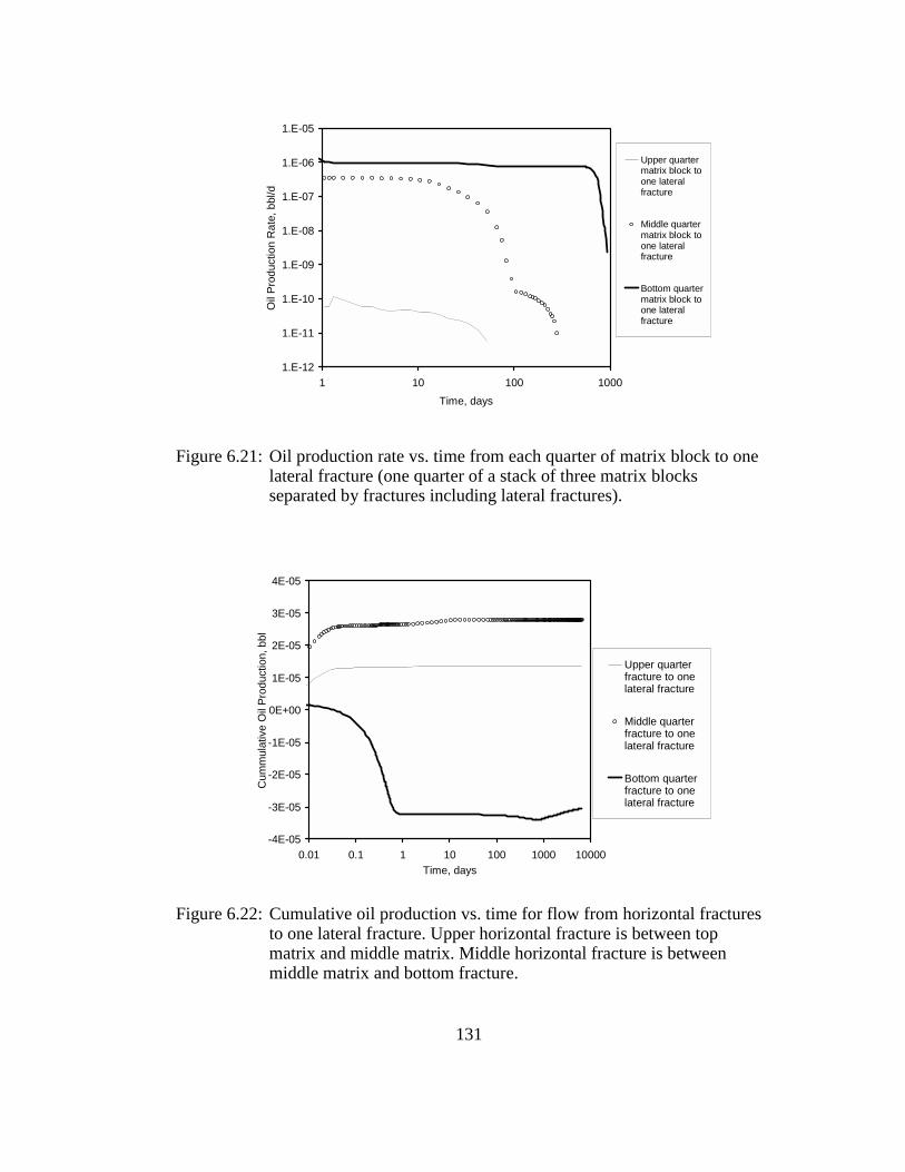
131

Figure 6.21: Oil production rate vs. time from each quarter of matrix block to one lateral fracture (one quarter of a stack of three matrix blocks separated by fractures including lateral fractures).

Figure 6.22: Cumulative oil production vs. time for flow from horizontal fractures to one lateral fracture. Upper horizontal fracture is between top matrix and middle matrix. Middle horizontal fracture is between middle matrix and bottom fracture.

1.E-12

1.E-11

1.E-10

1.E-09

1.E-08

1.E-07

1.E-06

1.E-05

1 10 100 1000

Time, days

Oil

Prod

uctio

n R

ate,

bbl

/d

Upper quartermatrix block toone lateralfracture

Middle quartermatrix block toone lateralfracture

Bottom quartermatrix block toone lateralfracture

-4E-05

-3E-05

-2E-05

-1E-05

0E+00

1E-05

2E-05

3E-05

4E-05

0.01 0.1 1 10 100 1000 10000Time, days

Cum

mul

ativ

e O

il Pr

oduc

tion,

bbl

Upper quarterfracture to onelateral fracture

Middle quarterfracture to onelateral fracture

Bottom quarterfracture to onelateral fracture

132

Figure 6.23: Cumulative oil production vs. time for flow from matrix blocks to one lateral fracture (a quarter of a stack of three matrix blocks divided by fractures with lateral fractures).

Figure 6.24: Oil pressure in the matrix (cell adjacent to fracture) for a stack of a quarter of three matrix blocks divided by fractures (including lateral fractures).

0

100

200

300

400

500

600

700

800

90079 79.5 80 80.5 81

Oil Pressure, atm

Dep

th fr

om T

op o

f Upp

er M

atrix

, cm 0.000 Days (Initial

conditions)

0.105 Days and gasgradient

28247 Days

139515 Days

Oil Gradient

0E+00

1E-04

2E-04

3E-04

4E-04

5E-04

6E-04

7E-04

0.01 0.1 1 10 100 1000 10000Time, days

Cum

mul

ativ

e O

il P

rodu

ctio

n, b

bl

Upper quarter matrixblock to one lateralfracture

Middle quarter matrixblock to one lateralfracture

Bottom quartermatrix to one lateralfracture

133

Figure 6.25: Capillary pressure profiles at different times for a quarter of a stack of three matrix blocks with gravity drainage.

Figure 6.26: Oil saturation in the matrix (cell adjacent to the fracture) for a quarter of a stack of three matrix blocks separated by fractures (including lateral fractures).

0

100

200

300

400

500

600

700

800

9000.5 0.6 0.7 0.8 0.9

Oil Saturation

Dep

th fr

om T

op o

f Upp

er M

atrix

, cm 0.00 Days

(Initialconditions)776 Days

1872 Days

28247 Days

Static saturation(Infinite flowtime)

0

100

200

300

400

500

600

700

800

9000 0.05 0.1 0.15 0.2

Capillary Pressure, atm

Dep

th fr

om T

op o

f Upp

er M

atrix

, cm

0.00 Days (Initialconditions)

764 Days

1856 Days

10348 Days

139515 Days

Static

134

Chapter 7 Fine Grid and Dual Porosity Simulation

The previous chapter corroborates that in 3D flow with gravity drainage,

lateral flow is negligible with and without capillarity. This chapter analyzes a

stack of matrix blocks simulated with a fine grid in the x, y, and z directions,

comparing the results with those obtained from a dual porosity model using

pseudo oil relative permeability and pseudo capillary pressure functions as

established in Chapters 4 and 5. Additionally, flow from the stack of matrix

blocks is compared with flow obtained from an equivalent matrix block the same

size of the stack of matrix blocks. Finally, a lab experimental case considering a

stack of three matrix blocks is simulated in 1D vertical direction.

7.1 STACK OF FIVE MATRIX BLOCKS

Figure 7.1 shows a stack of five matrix blocks separated by fractures. In

the case of fine grid simulation the total system was divided in 20x20x106 cells in

x, y and z directions respectively. Lateral fractures were not considered due to

lateral flow being negligible with gravity segregation. The flow is in 1D in the

vertical direction. The simulation grid considers each horizontal fracture as a layer

dividing matrix blocks. At the top of the stack of matrix blocks was placed a

fracture with injector wells simulating gas at constant pressure. At the bottom of

the stack of matrix blocks were placed producer wells simulating oil production

with gravity drainage from the stack of matrix blocks at constant pressure. Table

7.1 shows data for the fine and dual porosity grids.

135

Wells simulating gas injection at top of the stack of matrix blocks were

placed in the top fracture of the stack and wells simulating oil production by

gravity drainage were placed in the bottom fracture of the stack. To reduce the

number of wells during simulation Fig. 7.2 shows variation of cumulative oil for a

matrix block with different number of wells at the bottom of the matrix block.

This figure shows that it is not necessary to use the total number of wells in the

bottom fracture to simulate gravity drainage due to the high permeability in the

fracture. In this case 20 distributed wells were used as injectors at the top fracture

and 20 distributed wells were used as producers at the bottom fracture.

Cumulative oil from the top matrix block, middle matrix block, and

bottom matrix block to their adjacent bottom fracture is shown in Fig. 7.3. The

deeper the matrix block, the more cumulative oil to its adjacent bottom fracture.

This is due to reinfiltration of oil from upper to lower matrix block through the

fracture separating both matrix blocks. The curve showing cumulative oil from

the top matrix block to its adjacent bottom fracture is four times as that presented

in Fig. 6.5, which was simulated with a quarter of a matrix-fracture block.

At the beginning of the cumulative oil (Fig. 7.3) there is a straight line

with slope 2.13x10-3 bbl/d. This rate corresponds to a matrix block with gravity

segregation completely saturated with oil and with potential,

136

zgg

c

∆∆=∆Φ ρ (7.1)

Substituting Eq. 7.1 into the Darcy equation,

co

roo g

gAkkq ρµ

∆= (7.2)

Barkve and Firoozabadin (1992) also shows Eq. 7.2. Substituting values from

Table 4.1 into Eq. 7.2 results in 16.14=oq cm3/h (2.13x10-3 bbl/d).

Figure 7.4 shows the stack of five matrix blocks for simulation with the

dual porosity model in Eclipse to compare with the gridded stack of five matrix

blocks. The first comparison run between the two systems was made using oil

relative permeability and capillary pressure as in Figs. 4.2 and 4.3, respectively.

Figure 7.5 shows oil rate for the gridded stack of matrix blocks and the dual

porosity stack of matrix blocks. At early times the oil rate given by the dual

porosity system is five times greater than the oil rate given by the gridded stack of

matrix block. This is because the dual porosity system transfers oil from all matrix

blocks to fracture since the beginning of gravity drainage and the gridded stack of

matrix blocks transfers oil from the top matrix to its adjacent lower fracture and

from that fracture to the lower matrix and so on.

137

Figure 7.6 shows oil rate from each matrix block to fracture with the dual

porosity system and the total oil rate transferred from matrix to fracture. This

shows that this dual porosity model has no oil imbibition from fracture to matrix

in the dual porosity system since the total oil rate is five times the oil rate given

by the individual matrix blocks and no oil rate goes from fracture to matrix.

Figure 7.7 shows oil rate from each matrix block to its adjacent lower fracture in

the gridded stack of five matrix blocks. This shows that contrary to the dual

porosity model, the gridded stack of matrix blocks shows “complete” oil

reinfiltration (imbibition) from upper to lower matrix. Also from Fig. 7.7, the

maximum oil rate given by Eq. 7.2 is not a function of the number of matrix

blocks stacked. Duration and declination of the maximum flow rate depends on

the number of matrix blocks stacked.

7.2 SIMULATION WITH PSEUDO FUNCTIONS

To compare results with the gridded stack of matrices and the stack of

matrices simulated with dual porosity model given in Eclipse, the pseudo oil

relative permeability presented in Chapter 4 and the pseudo capillary pressure

given in Chapter 5 are used. The pseudo saturation functions utilized are in Fig.

4.19 for the pseudo oil relative permeability, and Fig. 5.27 for the pseudo

capillary pressure.

To activate the pseudo functions in the dual porosity model in Eclipse, the

first step is to activate a gravity segregation model in Eclipse (i.e. Model 1).

138

Secondly, determine the relative permeability accordingly to the established in

Chapter 4 and detailed in Chapter 6. In the Eclipse dual porosity model,

∆∆−−=

comDcm

o

romo g

gzSPkk ρµ

στ (7.3)

and the Bech et al. model neglecting gas viscous pressure gradient,

∆∆−=

comDcm

omDo

romo g

gzSPSkk ρ

µστ (7.4)

From Eqs. 7.3 and 7.4 the oil relative permeability used in Eclipse for

using the Bech et al. model,

omD

roeclipsero S

kk =, (7.5)

Pseudo capillary pressure is determined according to procedures in

Chapter 5 and detailed in Chapter 6. Figures 7.8 and 7.9 shows the modified

pseudo oil relative permeability and pseudo capillary pressure, respectively.

Figure 7.10 shows results with the gridded system for a stack of five

matrix blocks and those obtained with the dual porosity model with pseudo

functions. The Eclipse dual porosity model produces five times greater than the

transfer function given by the gridded model. This is because the gridded stack of

139

matrix blocks reproduces reinfiltration of oil. The dual porosity model in Eclipse

does not reproduce reinfiltration (imbibition). The gridded system gives oil

production at short times accordingly to Eq. 7.2. The matrix blocks then decline

oil rate gradually (first the top matrix block then the second and so on).

7.2.1 Matrix Block with the Same Size as a Stack of Five Matrix Blocks

Figure 7.11 shows saturation profile obtained with a gridded matrix block

of the same size of the stack of five matrix blocks. Figure 7.12 shows oil

production rate for both the stack of five matrix blocks and a matrix block of the

same size of the stack of five matrix blocks. The difference between both runs

happens because the matrix block of the same size as five matrix blocks produces

more oil when gas arrives at the bottom of the matrix block. Saturation profiles

given by the gridded five matrix blocks are in Fig. 7.14. Figures 7.14 and 7.15

show oil pressure at different times for the gridded stack of five matrix blocks and

the gridded matrix block of the same size as the stack of five matrix blocks.

From Figs. 7.11 and 7.13, there is a difference in oil saturation left in the

matrix after infinite time of gravity drainage accordingly to the height of the

matrix block. Figure 7.16 shows remaining oil saturation vs. matrix size in a

matrix block after infinite time. The higher the matrix block, the less oil left in the

matrix. Equation E.10 from Appendix E was used to do the calculations. This

figure also shows the static oil saturation given by capillary pressure.

140

7.2.2 Laboratory Measurements of Gravity Drainage

There are some gravity drainage experiments, one of the most documented

is by Firoozabadi (1993) that presented gravity drainage tests on a Berea

Sandstone block 1.815 m long with a cross sectional area of 229.5 cm2. The

experiments, he conducted with normal decane (nC10) allowing flow of

atmospheric air at the top. Table 7.1 shows the information of the matrix block,

capillary pressure, and oil relative permeability. Firoozabadi sectioned the matrix

block vertically in three equal matrix blocks of 60.5 cm long each. He put the

three matrix blocks in a stack and laced dividers between them allowing fractures

of 100 mµ aperture.

For the stack of three matrix blocks, Fig. 7.17 shows oil production rate

vs. time compared with the simulation results. Figure 7.18 shows cumulative oil

production from Eclipse and the Firoozabadi lab results. 1D vertical simulation

was utilized in Eclipse.

In summary, this chapter compares results from simulating a stack of five

matrix blocks with fine grid and results of the Eclipse dual porosity model. At

early times, the Eclipse dual porosity model with pseudo functions gives five

times greater flow rate than that obtained from a gridded stack of five matrix

blocks due to the fact that reinfiltration dominates in gravity drainage and the dual

porosity models consider only flow from matrix to fracture. A maximum oil flux

with gravity drainage is obtained with Darcy’s equation using the end point oil

141

relative permeability and the density difference between oil and gas instead of the

derivative of oil potential. Duration and declination of maximum oil flux depends

on the size and number of blocks stacked. At late flow times, oil rate from a stack

of five matrix blocks gives less oil rate than that obtained from a matrix block the

same size of the stack. Finally, an acceptable match is obtained simulating 1D

vertical flow with gravity drainage and a fine grid stack of three matrix blocks of

a laboratory gravity drainage experiment by Firoozabadi (1993).

142

Table 7.1: Data from Firoozabadi (1993) experiment at surface conditions (using air from the atmosphere instead of gas) for gravity drainage in a stack of three matrix blocks separated by fractures.

Description Value

Tall matrix block length, m 1.815

Sectioned matrix block length, cm 60.5

Bottom cross section area, cm2 229.5=(15.152)

Porosity, fraction 0.216

Permeability at bottom of tall

matrix block, md

754

Permeability at top of tall matrix

block, md

406

Oil density, gm/cc 0.724

Oil viscosity, cp 0.866

Residual oil saturation, fraction 0.26

Oil relative permeability, fraction 5.3

1

−−=

or

ororo S

SSk

Capillary pressure in matrix, atm

−−−=

or

orocm S

SSP1

ln17.19.2325.101

1

Capillary pressure in fracture, atm ( )[ ]{ }21.0ln0081.215.0325.101

1 −−= ocf SP

143

Figure 7.1 Stack of five matrix blocks separated by fractures. There are also fractures at top and bottom of the stack.

Fracture

Fracture

Fracture

Fracture

Fracture

Fracture

Matrix

Matrix

Matrix

Matrix

Matrix

Gas at Constant Pressure

Oil Production by Gravity Drainage

Fracture

Fracture

Fracture

Fracture

Fracture

Fracture

Matrix

Matrix

Matrix

Matrix

Matrix

Gas at Constant Pressure

Oil Production by Gravity Drainage

144

Figure 7.2: Cumulative oil from a matrix block flowing to bottom fracture for different number of wells placed at bottom fracture (matrix grid 11x11x22).

Figure 7.3: Total cumulative oil production from matrix blocks to their adjacent lower fracture in a stack of 5 matrix blocks separated by fractures.

0

2

4

6

8

10

12

0 1000 2000 3000 4000 5000 6000 7000 8000 9000Time, days

Cum

ulat

ive

Oil

Prod

uctio

n, b

bl

Matrix at top of the stack to its lowerfractureMatrix at middle of the stack to itslower fractureMatrix at bottom of the stack to itslower fracture

0

0.1

0.2

0.3

0.4

0.5

0.6

0 1000 2000 3000 4000 5000 6000 7000Time, days

Cum

ulat

ive

Oil

Pro

duct

ion,

bbl

145

Figure 7.4: Dual porosity model of 5 matrix blocks with its fractures utilized to compare the fine grid system.

300 cm

300 cm

300 cm

300 cm

300 cm

Matrix

Matrix

Matrix

Matrix

Matrix

Fracture

Fracture

Fracture

Fracture

Fracture

300 cm

300 cm

Fracture

Fracture

300 cm

300 cm

300 cm

300 cm

300 cm

Matrix

Matrix

Matrix

Matrix

Matrix

Fracture

Fracture

Fracture

Fracture

Fracture

300 cm

300 cm

Fracture

Fracture

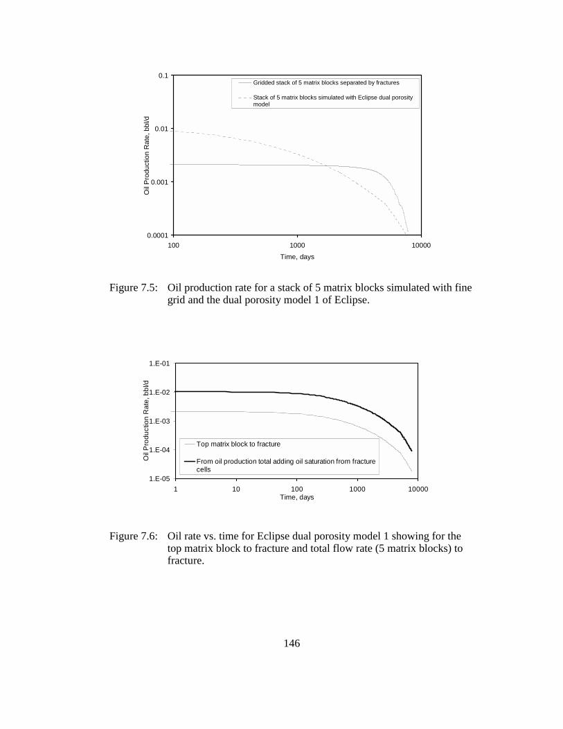
146

Figure 7.5: Oil production rate for a stack of 5 matrix blocks simulated with fine grid and the dual porosity model 1 of Eclipse.

1.E-05

1.E-04

1.E-03

1.E-02

1.E-01

1 10 100 1000 10000Time, days

Oil

Pro

duct

ion

Rat

e, b

bl/d

Top matrix block to fracture

From oil production total adding oil saturation from fracturecells

Figure 7.6: Oil rate vs. time for Eclipse dual porosity model 1 showing for the top matrix block to fracture and total flow rate (5 matrix blocks) to fracture.

0.0001

0.001

0.01

0.1

100 1000 10000Time, days

Oil

Pro

duct

ion

Rat

e, b

bl/d

Gridded stack of 5 matrix blocks separated by fractures

Stack of 5 matrix blocks simulated with Eclipse dual porositymodel

147

Figure 7.7: Oil production rate for each matrix block to its adjacent lower fracture for a stack of 5 matrix blocks. Simulated with fine grid model.

Figure 7.8: Pseudo oil relative permeability used in the dual porosity simulation in Eclipse dual porosity model to simulate a stack of 5 matrix blocks.

0.0

0.2

0.4

0.6

0.8

1.0

1.2

1.4

1.6

0.4 0.5 0.6 0.7 0.8 0.9Oil Saturation

Pse

udo

Oil

Rel

ativ

e P

erm

eabi

lity

Oil relative permeability with eo=3

Pseudo oil relative permeability (oilrelative permeability divided by oilsaturation)

1.E-05

1.E-04

1.E-03

1.E-02

100 1000 10000Time, days

Oil

Rat

e fro

m M

atrix

to it

s A

djac

ent B

otto

m

Frac

ture

, bbl

/d

Matrix at top of the stack to itslower fracture

Matrix at middle of the stack toits lower fracture

Matrix at bottom of the stack toits lower fracture

148

Figure 7.9: Pseudo capillary pressure obtained with the procedures of Chapter 5.

Figure 7.10: Oil rate vs. time for a gridded stack of 5 matrix blocks and the same stack simulated with Eclipse dual porosity model using pseudo oil relative permeability and pseudo capillary pressure.

-0.02

-0.01

0.00

0.01

0.02

0.03

0.04

0.05

0.4 0.5 0.6 0.7 0.8 0.9Oil Saturation

Pse

udo

Cap

illar

y P

ress

ure,

atm

1.E-05

1.E-04

1.E-03

1.E-02

1.E-01

100 1000 10000 100000Time, days

Oil

Rat

e, b

bl/d

Gridded stack of 5 matrix blocks separated by fractures

Stack of matrix blocks with dual porosity, pseudo oilrelative permeability, and pseudo capillary pressure

149

Figure 7.11: Oil production of a gridded stack of 5 matrix blocks and a matrix block of equal size of the stack of 5 matrix blocks.

Figure 7.12: Oil saturation profiles in a matrix block of size equal to a stack of five matrix blocks flowing with gravity drainage.

1.E-05

1.E-04

1.E-03

1.E-02

100 1000 10000 100000Time, days

Oil

Pro

duct

ion

Rat

e, b

bl/d

Gridded stack of 5 matrix blocks separated by fractures

One matrix block with same size of a stack of 5 matrix blocks (gridded)

0

200

400

600

800

1000

1200

1400

0.5 0.6 0.7 0.8 0.9

Oil Saturation

Dep

th fr

om T

op o

f Mat

rix, c

m 0 days (Initialconditions)

601 days

3539 days

11048 days

23761 days

Static

150

Figure 7.13: Oil saturation profiles at different times for the gridded stack of five matrix blocks.

Figure 7.14: Oil pressure profiles at different times for the gridded stack of five matrix blocks.

0

200

400

600

800

1000

1200

1400

0.6 0.65 0.7 0.75 0.8 0.85 0.9

Oil Saturation

Dep

th fr

om T

op o

f Sta

ck o

f Mat

rix B

lock

s, c

m

0.00 days

442 days

2017 days

4513 days

22848 days

0

200

400

600

800

1000

1200

1400

79.6 79.8 80.0 80.2 80.4 80.6 80.8 81.0 81.2 81.4

Oil Pressure, atm

Dep

th fr

om T

op o

f Sta

ck o

f Mat

rix B

lock

s, c

m 0.00 days (Initialconditions)

4.17 days and gas gradient

4513 days

22848 days

151

Figure 7.15: Oil pressure profiles at different times for the gridded matrix block with same size that the stack of five matrix blocks.

Figure 7.16: Remaining oil saturation vs. size of matrix blocks and static oil saturation given by capillary pressure.

0

200

400

600

800

1000

1200

1400

78.5 79 79.5 80 80.5 81 81.5

Oil Saturation

Dep

th fr

om T

op o

f Mat

rix, c

m 0 days (Initialconditions)

Gas gradientand 3 days

3538.747917days

11047.70417days

23760.62083days

Oil gradient

0

1000

2000

3000

4000

5000

6000

7000

8000

9000

0.4 0.45 0.5 0.55 0.6 0.65 0.7 0.75 0.8 0.85 0.9Oil Saturation

Mat

rix H

eigh

t fro

m B

otto

m o

f Mat

rix, c

m

Average oil saturation remaining in the matrix block

Static oil saturation

152

Figure 7.17: Oil production rate vs. time for a stack of three matrix blocks with gravity drainage from Firoozabadi (1993) experiments and 1D simulation with Eclipse.

Figure 7.18: Cummulative oil production vs. time for a stack of three matrix blocks with gravity drainage from Firoozabadi (1993) experiments and 1D simulation with Eclipse.

1.E-02

1.E-01

1.E+00

1.E+01

1.E+02

1.E+03

1.E+04

1 10 100 1000 10000 100000Time, hrs

Oil

Pro

duct

ion

Rat

e, c

c/hr

Firoozabadi experiment

Eclipse simulation

0

500

1000

1500

2000

2500

1 10 100 1000 10000 100000Time, hrs

Cum

mul

ativ

e O

il Pr

oduc

tion,

cc

Firoozabadi experimentEclipse simulation

153

Chapter 8 Conclusions and Recommendations

The following conclusions and recommendations were derived from this

study.

8.1 CONCLUSIONS

1. For dual porosity models a procedure is established to determine

pseudo oil relative permeability and pseudo capillary pressure with

and without fine grid simulation of a matrix block.

2. The pseudo oil relative permeability is calculated with the Corey

exponent of a real oil relative permeability and it can also be

calculated with oil relative permeability in tabular form.

3. The Beck et al. dual porosity model better represents oil transfer

from matrix to fracture than others dual porosity models.

4. In 3D flow with gravity drainage the flow in the lateral direction is

negligible.

5. In a matrix block with gravity drainage, oil flux from opening 75%

or more of the bottom face of the matrix block is similar to oil flux

with a complete bottom face opened to flow. When flow has

restrictions at the bottom of the matrix block flow goes to lateral

fractures.

154

6. In 3D flow in a stack of matrix blocks separated by fractures, oil

reinfiltrates from upper to lower matrix blocks with negligible oil

flow to the lateral direction.

7. Maximum oil flux at the bottom of a stack of any number of matrix

blocks with gravity drainage is given by Darcy’ law using the end

point oil relative permeability and the difference of fluid densities

for the derivative of potential. At early times there is a maximum

oil flux with gravity segregation. The duration and decline of this

oil flux depends on the number and height of blocks stacked.

8. Gas viscous pressure drops have major influence in oil flux in

zones of first contact of gas with oil (low gas saturation zones).

Neglecting gas viscous pressure drop is not meaningful in gridded

matrix block simulations. Neglecting gas mobility in dual porosity

models match closely with gridded matrix blocks simulations.

9. A model in 1D in vertical direction accurately represents gas-oil

flow with gravity drainage in 2D or 3D flow, for one matrix block

and for a stack of matrix blocks.

8.2 RECOMMENDATIONS

1. Due to oil reinfiltration it is recommendable to test Bech et al.

model in dual permeability simulators, which consider matrix-

matrix oil transfer.

155

2. Due to oil flow is mainly vertical from upper to lower matrix

blocks it is convenient to determine gravity drainage in inclined

stack of matrix blocks in order to evaluate partial reinfiltration

from upper to lower matrix blocks.

156

APPENDIX A Solution to 1D Vertical Gravity Drainage

Equation 4.33 is a second order non-linear partial differential equation for

flow of gravity drainage considering negligible viscous pressure drop in the gas

phase. This Appendix shows the solution of this equation with the finite

difference method. The equation to solve is

01 =

−

∂∂

∂∂+

∂∂

D

croD

DD

oD

zP

kzt

S (A.1)

Initial and boundary conditions are

( ) 10, ==DDoD tzS (A.2)

1=∂∂

topD

cD

zP

(A.3)

0=bottomcDP (A.4)

Applying finite differences and considering block-centered grids (Fig.

A.1),

157

0111

2/12/1

,, =

−

∂∂

−

−

∂∂

∆+

∆−

−+ iD

cDroD

iD

cDroD

Di

nioDioD

zP

kzP

kzt

SS (A.5)

Developing the terms in brackets gives

tSS n

ioDioD

∆− ,, ( )

∆−−

∆∆+ ++

+2/1,,1,

2/1

1iDicDicD

iD

roD

Di

zPPz

kz

( ) 02/1,1,,2/1

=

∆−−

∆− −−

−iDicDicD

iD

roD zPPz

k (A.6)

Using the implicit method for solving this equation, the terms oDS , cDP ,

and roDk are evaluated at time 1+n . If all Dz∆ are equal,

( )2Dztr

∆∆= (A.7)

Substituting Eq. A.7 into Eq. A.6 gives

( )[ DicDicDiroDn

ioDioD zPPkrSS ∆−−+− ++ ,1,2/1,,,

( )] 01,,2/1, =∆−−− −− DicDicDiroD zPPk (A.8)

Equation A.8, for cells 2 and 3, respectively, gives

( )[ DcDcDroDnoDoD zPPkrSS ∆−−+− + 2,3,2/12,2,2,

158

( )] 01,2,2/12, =∆−−− − DcDcDroD zPPk (A.9)

and

( )[ DcDcDroDnoDoD zPPkrSS ∆−−+− + 3,4,2/13,3,3,

( )] 02,3,2/13, =∆−−− − DcDcDroD zPPk (A.10)

Equations for the first cell (bottom) and the last cell (top) include

boundary conditions. Development for cell one from Eq. A.1 and using a block-

centered grid using the distance from the bottom boundary to the center of the cell

as 2/z∆ , gives

( )

∆−−

∆∆+

∆−

+DcDcD

D

roD

D

noDoD zPP

zk

ztSS

1,2,2/11

1,1, 1

012/

2/11,1,2/11

=

−

∆−

− −−

D

cDcDroD z

PPk (A.11)

The boundary condition at cell one is 02/11, =−cP . Substituting the value of

r given by Eq. A.7 in Eq. A.11 gives

( ) ( )[ ] 02 1,2/11,1,2,2/11,1,1, =∆−−∆−−+− −+ DcDroDDcDcDroDnoDoD zPkzPPkrSS (A.12)

An equivalent form of Eq. A.5 for cell N gives

159

0111

2/12/1

,, =

−

∂∂

−

−

∂∂

∆+

∆−

−+ ND

cDroD

ND

cDroD

D

nNoDNoD

zPk

zPk

ztSS

(A.13)

The boundary condition at the top of the matrix is 1=∂∂

D

cD

zP

. Substituting

in Eq. A.13 gives

012/1

,, =

−

∂∂

−∆∆+−

−ND

cDroD

D

nNoDNoD z

PkztSS (A.14)

Expanding the spatial derivative,

011,,2/1,, =

−

∆−

−∆∆+− −

−D

NcDNcDNroD

D

nNoDNoD z

PPk

ztSS (A.15)

Substituting r from Eq. A.7 into Eq. A.15,

( )[ ] 01,,2/1,, =∆−−−+− −− DNcDNcDNroDn

NoDNoD zPPkrSS (A.16)

Derivatives of each cell equation are taken with respect to saturation in

order to construct a matrix of derivatives (Jacobian matrix) are

( )2/11,2/11,'

1,11,

1 21 −+ +−=∂

∂roDroDcD

oD

kkPrS

f (A.17)

160

2/11,'

2,12,

1+=

∂∂

roDcDoD

kPrS

f (A.18)

2/12,'

1,21,

2−=

∂∂

roDcDoD

kPrS

f (A.19)

( )2/12,2/12,'

2,22,

2 1 −+ +−=∂

∂roDroDcD

oD

kkPrS

f (A.20)

2/12,'

3,23,

2+=

∂∂

roDcDoD

kPrS

f (A.21)

.

.

.

2/1,'

1,1,

−−−

=∂

∂NroDNcDN

NoD

N kPrS

f (A.22)

2/1,'

,1 −−=∂∂

NroDNcDNoDN

N kPrSf (A.23)

where roDk is evaluated upstream and 1f , 2f , 3f , and nf are the equations A.12,

A.9, A.10, and Eq. A.16, respectively.

Eq. 4.43 represents oil flux at any position in the matrix, then oil flux at

the outlet of the matrix block in finite difference form,

161

−

∆−

= −−− 1

2/2/11,1,

2/11,2/11,D

cDcDroDoD z

PPku (A.24)

where 02/11, =−cDP represents capillary pressure at the lower boundary of the

matrix. Considering this in Eq. A.24 gives

−

∆= −− 1

2 1,2/11,2/11,

D

cDroDoD z

Pku (A.25)

or

( )DcDD

roDoD zP

zk

u ∆−∆

= −− 1,

2/11,2/11, 2 (A.26)

This equation is solved at time 1+n just after each saturation is calculated

with the implicit model.

162

Figure A.1: Block centered grid used to numerically solve Eq. 4.33 in one dimension in the vertical direction.

∆zD7-1/2

12

3

19

20

∆zD1-1/2

∆zD3

PcD=0

1=∂∂

D

cD

zP

∆zD7-1/2

12

3

19

20

∆zD1-1/2

∆zD3

PcD=0

1=∂∂

D

cD

zP

163

APPENDIX B: Dimensionless Form of Transfer Function

This appendix shows the oil transfer function in dimensionless form.

From Eq. 4.39,

∆−

∂∂

=c

c

o

roo g

gzPAkk

q ρµ

(B.1)

Dividing by bulk volume, bV , and defining,

b

oo V

q=τ (B.2)

Substituting Eq. B.2 into Eq. B.1,

∆−

∂∂

=c

c

bo

roo g

gzP

VAkk ρ

µτ (B.3)

To transform Eq. B.3 to dimensionless form, first multiply by hh / and

group terms,

∆−

∂∂

= hgg

zP

kkA

hV

cD

cro

obo ρτµ (B.4)

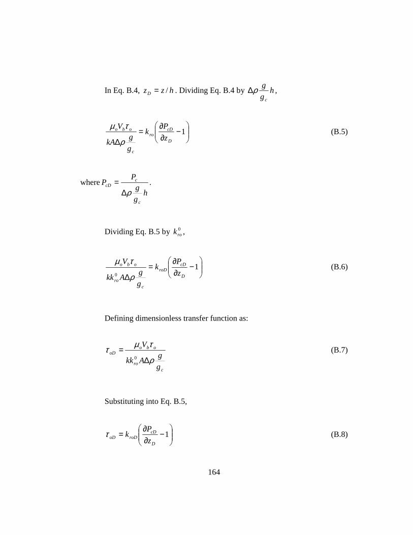
164

In Eq. B.4, hzzD /= . Dividing Eq. B.4 by hgg

c

ρ∆ ,

−

∂∂

=∆

1D

cDro

c

obo

zP

k

ggkA

V

ρ

τµ (B.5)

whereh

gg

PP

c

ccD

ρ∆= .

Dividing Eq. B.5 by 0rok ,

−

∂∂

=∆

10 D

cDroD

cro

obo

zP

k

ggAkk

V

ρ

τµ (B.6)

Defining dimensionless transfer function as:

cro

obooD

ggAkk

V

ρ

τµτ∆

=0

(B.7)

Substituting into Eq. B.5,

−

∂∂

= 1D

cDroDoD z

Pkτ (B.8)

165

Appendix C Height of Oil and Gas with Vertical Equilibrium

This Appendix determines the vertical section of each phase in a matrix

block based on vertical equilibrium and total fluid segregation. This phase vertical

section of is used in matrix or fracture blocks for dual porosity models with flow

in 1D vertical direction.

Aziz et al. (1999) establishes that for vertical fluid distribution due to

gravity equilibrium the average saturation of a phase p is determined by

( ) ( )

( )∫∫= h

h

pp

dzz

dzzSzS

0

0

φ

φ (C.1)

For a totally segregated gas-oil system with gravity drainage and

considering constant porosity, initial gas, and initial water saturation in Eq. C.1

(Fig. C.1),

( ) ( )[ ]ogiwiooo hSShhSh

S −−+−= 11min (C.2)

Where h is the height of the matrix block and oh is the oil height in the

matrix block. Developing Eq. C.2,

( )wigiooooo SShShhShS −−+−= 1minmin (C.3)

166

Obtaining oh ,

wigio

ooo SSS

SShh

−−−−

=min

min

1 (C.4)

For the gas phase,

( ) ( )[ ]ggigwiog hhShSSh

S −+−−= min11 (C.5)

Where gh is the gas height in the matrix block. Developing Eq. C.5,

( ) ggigigwiog hShShSShS −+−−= min1 (C.6)

Obtaining gh ,

wigio

gig

g SSSSS

hh−−−

−=

min1 (C.7)

For a water-oil system with initial gas saturation and from Fig. C.1,

( ) ( )[ ]ooogiwio hhShSSh

S −+−−= min11 (C.8)

Developing,

167

( ) oooogiwio hShShSShS minmin1 −+−−= (C.9)

Obtaining oh ,

wigio

ooo SSS

SShh

−−−−

=min

min

1 (C.10)

Equation C.10 is the same as Eq. C.4. The average water saturation,

( ) ( )[ ]wgiowwiw hSShhSh

S −−+−= min11 (C.11)

Where wh is the water height in the matrix block. Developing Eq. C.11,

( ) wgiowwiwiw hSShShShS −−+−= min1 (C.12)

Obtaining wh

giwio

wiww SSS

SShh

−−−−

=min1

(C.13)

Equations C.4, C.7, and C.13 were also presented by Sonier et al. (1986).

Figure C.2 shows variation of oh with respect to average oil saturation. It is

important to consider minoS instead of orS in Eqs. C.4, C.7, and C.13. Figure C.2

168

shows calculations of the oil height in the matrix block considering minoS and

orS . For a saturation value, calculations using orS gives greater oil height values

than using minoS . In a matrix block the minimum oil saturation at infinite time of

simulation will be minoS and will never reach orS . Therefore, calculations with

orS will over estimate oil saturations at vertical equilibrium.

These equations can be used for fracture or matrix. For the purpose of this

study 0=giS , therefore Eqs. C.4, C.7, and C.13 for matrix and dividing by h , are

the same as definitions of dimensionless variables for oil, gas, and water,

respectively;

wimo

oomomoD SS

SSh

hS−−

−==

min

min

1 (C.14)

wimo

gmgmgD SS

Sh

hS

−−==

min1 (C.15)

wimo

wiwmwmwD SS

SSh

hS−−

−==

min1 (C.16)

169

Figure C.1: Representation in vertical equilibrium of saturation of fluids in a matrix block at initial conditions, in a gas-oil system and in a water-oil system, Aziz et al. (1999).

0 1

Som in 1-Swi

0 1

Som in 1-Swi

hg

ho

a) M atrix block saturated with oil, initial water, and initial gas b) M atrix block saturated with oil, gas, and initial water

h

1-Swi-Sgi 1-Swi-Sgi

So So

0 1

Som in 1-Swi

0 1

Som in 1-Swi

hg

ho

a) M atrix block saturated with oil, initial water, and initial gas b) M atrix block saturated with oil, gas, and initial water

h

1-Swi-Sgi 1-Swi-Sgi

So So

0 1

Somin 1-Sgi

ho

hw

c) Matrix block saturated with oil, water, and initial gas

∆zm

1-Swi-Sgi

So

0 1

Somin 1-Sgi

ho

hw

c) Matrix block saturated with oil, water, and initial gas

∆zm

1-Swi-Sgi

So

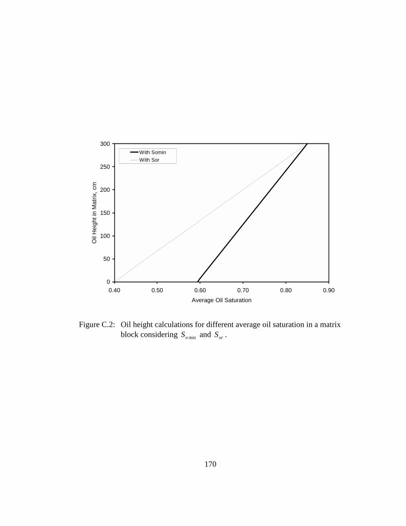
170

Figure C.2: Oil height calculations for different average oil saturation in a matrix block considering minoS and orS .

0

50

100

150

200

250

300

0.40 0.50 0.60 0.70 0.80 0.90Average Oil Saturation

Oil

Hei

ght i

n M

atrix

, cm

With SominWith Sor

171

Appendix D Dimensionless Form of Dual Porosity Models

Chapter 5 shows the development of gravity drainage dual porosity

models. This Appendix shows the development of these dual porosity models in

dimensionless form.

D.1 ECLIPSE MODEL

To transform Eq. 5.17 into dimensionless form, first divide by 0ro

c

kggz ρ∆∆ , considering 1=gfDS , gmDoD SS −=1 , and rearranging terms,

∆∆−=

∆∆c

cmoD

ro

ro

crom

oo

ggz

PS

kk

ggzkk ρρσ

τµ0

0 (D.1)

Defining

o

crom

ooD

ggzkk

τσρ

µτ∆∆

=0

(D.2)

Additionally, roDk and cmDP are defined by Eqs. 4.27 and 4.29,

respectively ( oDS is defined by Eq. 5.20). Substituting Eqs. D.2, 4.27, and 4.29

into Eq. D.1,

172

( )cmDoDroDoD PSk −=τ (D.3)

To transform Eq. 5.19 to dimensionless form, first divide Eq. 5.18 by

cro g

gzk ρ∆∆0 and substitute Eq. 4.29 into Eq. 5.18,

( )cmDoDroDo

crom

o PSkdt

dS

ggzkk

−−=∆∆ ρσ

φµ0

(D.4)

Considering, ( )minooo SS

dtd

dtdS

−= , multiplying Eq. D.4 by

( ) ( )wiowio SSSS −−−− minmin 1/1 , and substituting oDS given by Eq. 5.20,

( ) ( )cmDoDroD

oD

crom

owio PSkdt

dS

ggzkk

SS−−=

∆∆

−−

ρσ

φµ0

min1 (D.5)

Defining Dt by

( ) tSS

ggzkk

towio

crom

D φµ

ρσ

−−

∆∆=

min

0

1 (D.6)

Considering the definition of σ (Eq. 5.31), Eq. D.6 is very similar to Eq.

4.32. Substituting Eq. D.6 in Eq. D.5,

173

( )oDcmDroDD

oD SPkdt

dS−= (D.7)

Integrating Eq. D.7,

( )( )

∫ −= DoD tS

oDcmDroD

oDD SPk

dSt

0 (D.8)

which is Eq. 5.19 in dimensionless form.

D.2 QUANDALLE AND SABATHIER MODEL

Dividing Eq. 5.47 by zgg

c

∆∆ρ and considering 0=cfP ,

−∆∆

−=∆∆ 2

12z

gg

Pk

zgg

c

cmzrom

c

oz

ρσλ

ρ

τ (D.9)

Dividing by 0rok and substituting the definitions of roDk and cmDP (Eqs.

4.27 and 4.29) into Eq. D.9,

−−=

∆∆ 212

0cmDz

o

roDm

cro

oz Pk

kz

ggk

σµρ

τ (D.10)

174

Arranging terms and substituting Eq. D.2 into Eq. D.10,

−= cmDroDoD Pk

212τ (D.11)

To transform Eq. 5.49 to dimensionless form, first multiply Eq. 5.48 by

( ) ( )wiowio SSSS −−−− minmin 1/1 ,

( )

∆∆−−=−−2

21 min

zggPP

kkdt

dSSS

ccfcm

o

zromoDwio ρ

φµσ

(D.12)

Dividing by zggk

cro ∆∆ρ0 and considering 0=cfP in Eq. D.12,

−∆∆

=∆∆

−−2121

00

min

zgg

Pk

kkdt

dS

zggk

SS

c

cm

roo

zromoD

cro

wio

ρφµσ

ρ (D.13)

Substituting Eqs. 4.27 and 4.29 into Eq. D.13,

( )

−=

∆∆

−−212

10

mincmDroD

oD

zc

rom

wioo Pkdt

dS

zggkk

SS

σρ

φµ (D.14)

Substituting Eq. D.6 into Eq. D.14,

175

−=

212 cmDroD

D

oD Pkdt

dS (D.15)

Separating variables and integrating,

( )

∫

−

= DoD tS

cmDroD

oDD

Pk

dSt

0

212

(D.16)

which is Eq. 5.49 in dimensionless form.

D.3 BECH ET AL. MODEL

Considering 0=cfP in Eq. 5.96, dividing by zkgg

roc

∆∆ 0ρ , and grouping

terms,

∆−

−∆∆

−=∆∆ z

zz

zgg

pSkk

ggzkk

gmgf

c

cm

omDro

ro

crom

oo

ρσρ

τµ0

0 (D.17)

From Appendix C, gfDgf zSz ∆= , gmDgm zSz ∆= , considering 1=gfz ,

gmoD zz −=1 , and substituting Eqs. 4.27, 4.29, and Eq. D.2 into Eq. D.17,

( )oDcmDoD

roDoD SP

Sk

−−=τ (D.18)

176

To transform Eq. 5.98 to dimensionless form, first substitute

( )minooo SS

ttS

−∂∂=

∂∂

into Eq. 5.97, multiply by ( ) ( )wiowio SSSS −−−− minmin 1/1 ,

divide by c

ro ggzk ρ∆∆0 , and substitute Eq. 5.20,

( ) ( )omDcmD

omD

roDoD

crom

owio SPSk

tS

ggzkk

SS−=

∂∂

∆∆

−−

σρ

φµ0

min1 (D.19)

Substituting Eq. D.6 into Eq. D.19,

( )omDcmDomD

roD

D

oD SPSk

dtdS

−= (D.20)

Separating variables and integrating

( )( )

∫−

= DoD tS

omDcmDomD

roD

oDD

SPSk

dSt

0 (D.21)

which is Eq. 5.98 in dimensionless form.

177

Appendix E Oil Saturation Due to Capillarity

This Appendix shows the determination of average saturation distribution

in the matrix at static conditions due to capillarity.

E.1 AVERAGE SATURATION DISTRIBUTION IN THE MATRIX BLOCK AT STATIC CONDITIONS

Figure 4.5 shows dimensionless capillary pressure. An analytical equation

is given in Table 4.2:

( ) pceoDcDcD SPP −= 10 (E.1)

where cDP is defined by Eq. 4.29, oDS is defined by Eq. 4.28, and 0cDP is

defined by the following equation:

hgg

PP

c

ccD

ρ∆=

00 (E.2)

Capillary pressure at static conditions,

hggP

cc ρ∆= (E.3)

Dividing Eq. E.3 by zgg

c

∆∆ρ results in

178

DcD hP = (E.4)

where z

gg

PP

c

ccD

∆∆=

ρ and

zhhD ∆

= . Substituting Eq. E.4 in E.1 and

integrating from zero to 1, oDS can be calculated by

( ) oDS

eoD

D

cDoDoD SdS

hPSS

oD

pc ~~110

minmin

∫ −+= (E.5)

where minoDS is dimensionless oil saturation at minimum saturation in the

matrix that corresponds to 1=Dh ( 1=cDP ). Solving the integration with a change

of variables,

( )

11 1

min0

min +−

+=+

pc

eoD

D

cDoDoD

eS

hP

SSpc

(E.6)

Considering 1=Dh (top of matrix),

( )

11 1

min0min +

−+=

+

pc

eoD

cDoDoDeS

PSSpc

(E.7)

Substituting values from Table 4.4 the second term in the RHS of Eq. E.7

is equal to 0.0814 and total average dimensionless oil saturation at static

conditions is 511.0=oDS .

179

The average oil saturation can thus be calculated with the following

equation.

∫−

−−−

−∆

+=wi

o

pcS

So

e

wior

oro

c

coo Sd

SSSS

ggh

PSS

10

min

min

~1

~1

ρ (E.8)

where minoS is oil saturation at top of the matrix with static conditions and oS~ is

an integration variable. Solving the integral by a change of variables,

( )1

min0

min 11

1)1(

+

−−−

−+−−

∆+=

pce

wior

oro

pc

wior

c

coo

SSSS

eSS

ggh

PSSρ

(E.9)

Substituting information from Tables 4.1 and 4.2 into Eq. E.9 gives

63.0=oS , which in dimensionless form results in 511.0=oDS .

180

Appendix F Gas Mobility Effects

In Chapter 4 the development of vertical flow with gravity drainage

considered negligible viscous pressure drop in the gas phase. In Chapter 5 the

analysis of the dual porosity models neglects the effect of gas mobility. This

Appendix analyses these effects.

F.1 NEGLECTING GAS VISCOUS FORCES

Figure F.1 shows oil flux of a gridded matrix block with gravity drainage

considering two different curves of gas relative permeability. One is given by the

Corey type equation considering a gas exponent ( ge ) equal to 2 and the end point

gas relative permeability ( 0rgk ) equal to 0.32 (Table 4.2). The other curve

corresponds to an “ideal” gas relative permeability (a straight line with slope

equal to 45 degrees).

Figure F.2 Shows oil flux using gas relative permeability with a straight

line and oil flux obtained with the vertical drainage equation, which neglects

viscous pressure drop in the gas phase. The match is better than considering gas

relative permeability represented with the Corey type equation with gas exponent

eg=2 (Table 4.2). Figure F.3 shows different saturation profiles at different times

using gas relative permeability represented by a straight line with slope equal to

45 degrees and the vertical drainage equation that neglects gas viscous pressure

drop. Figure 4.10 shows saturation profiles at different times using gas relative

181

permeability with the Corey type equation (eg=2). Comparing Figs. 4.10 of

Chapter 4 and F.3, using gas relative permeability represented by a straight line

matches better with the vertical gravity equation. Previous observations conclude

that using a straight line gas relative permeability is more like neglecting viscous

pressure drop in the gas phase.

F.2 NEGLECTING GAS MOBILITY

The term in the denominator of dual porosity models (Eqs. 5.15, 5.44, and

5.91) adds ratios of viscosity divided by relative permeability for oil and gas. Gas

viscosity is small compared with oil viscosity ( =gµ 0.015 cp, =oµ 3.14 cp), but

when gas saturation is very small (high oil saturation or beginning of gravity

drainage) gas relative permeability is also very small (krg=0.0002). This makes

rgg k/µ greater than and dominant compared with roo k/µ .

Figure F.4 shows roo k/µ and rgg k/µ . Modifying the gas relative

permeability exponent ( ge ) equal one such that the gas phase is more

“moveable,” the results are similar to Fig. F.4, but with the intersection between

curves slightly to the right hand side. Figure F.5 shows oil and gas mobility where

the intersection with both curves has relation with Fig. F.4, which means that gas

mobility is less than oil mobility at low gas saturations. Figure F.6 shows the

transfer function for the cases shown above. This makes a difference in the dual

porosity models at short times, but matches at long times when gas mobility

dominates oil mobility.

182

From oil flux in Figs. F.1 and F.2 and the previous observations, the dual

porosity models match better neglecting the gas mobility term. This is due to the

fact that in the gridded system, low gas mobility has more effect in the cells with

low gas saturation (first contact of oil by gas). However, the “general” behavior is

not greatly affected due to the low gas saturation cells are less in number

compared with the whole cells of the matrix block. In the case of dual porosity

models (one cell model) the low gas mobility effect is enhanced. Therefore the

low gas mobility effect must be neglected in dual porosity models.

183

Figure F.1: Oil flux vs. time modifying the gas relative permeability to a straight line of slope 45 degrees compared with the Corey type equation of Table 4.2.

Figure F.2: Oil flux vs. time from a matrix block with gravity drainage using a modified gas relative permeability with a straight line of 45 degrees and the vertical gravity equation neglecting gas viscous pressure drops.

1.E-07

1.E-06

1.E-05

1.E-04

100 1000 10000Time, days

Oil

Flux

, bbl

/d/ft

2

Gas relative permeability with an exponent (eg) equal 2and end point gas relative permeability equal 0.32

Modification of gas relative permeability to a straight linewith slope 45 degrees

1.E-07

1.E-06

1.E-05

1.E-04

100 1000 10000Time, days

Oil

Flux

, bbl

/d/ft

2

Modification of gas relative permeability to a straightline with slope 45 degrees

Vertical gravity equation neglecting gas viscouspressure drop

184

Figure F.3: Saturation profiles at different times for a matrix block with gravity drainage for a) using gas relative permeability with a straight line of 45 degrees and b) vertical gravity equation that neglects gas viscous pressure drops.

Figure F.4: Ratio gas viscosity/gas relative permeability and oil viscosity/oil relative permeability and addition of both ratios.

1E-02

1E-01

1E+00

1E+01

1E+02

1E+03

1E+04

0.40 0.50 0.60 0.70 0.80 0.90

Oil Saturation

Rat

io V

isco

sity

/Rel

ativ

e Pe

rmea

bilit

y, c

p

Oil viscosity divided by oil relative permeability

Gas viscosity divided by gas relative permeability

Addition of both ratios

0

50

100

150

200

250

300

0.5 0.55 0.6 0.65 0.7 0.75 0.8 0.85 0.9Oil Saturation

Mat

rix H

eigh

t fro

m B

otto

m o

f Mat

rix, c

m

Eclipse, 736 days (gas relativepermeability with a straight line ofslope equal to 45 degrees)

Eclipse, 2557 days (gas relativepermeability with a straight line ofslope equal to 45 degrees)

Vertical gravity equation, 729 days(Neglecting gas viscous pressuredrop)

Vertical gravity equation, 2553days (Neglecting gas viscouspressure drop)

Static

185

Figure F.5: Oil and gas mobility for the Corey type equation with oil and gas exponents equal to 3 and 2, respectively ( oe and ge ).

Figure F.6: Transfer function with the dual porosity model with and without gas mobility term. When including gas mobility term there are two cases of gas relative permeability exponent (eg=2, eg=1).

1.E-04

1.E-03

1.E-02

1.E-01

1.E+00

1.E+01

1.E+02

0.40 0.50 0.60 0.70 0.80 0.90Oil Saturation

Mob

ility

, 1/c

p

Oil mobility

Gas mobility

1E-08

1E-07

1E-06

1E-05

10 100 1000 10000Time, days

Tran

sfer

Fun

ctio

n, b

bl/d

/ft3

Bech et al. dual porosity model with no gas mobilityterm (Integral solution)Bech et al. dual porosity model including gas movilityterm, eg=2 (Integral solution)Beck et al. dual porosity model (including gas movilityterm, eg=1)

186

Appendix G Code in C++ and Eclipse File for Solving 1D Vertical Gravity Drainage

This appendix shows the code in C++ to solve 1D vertical gravity

drainage and the Eclipse data file to simulate the same case for vertical gravity

drainage.

G.1 C++ CODE FOR VERTICAL GRAVITY DRAINAGE IN 1D /* ================ Nemesio Miguel-H Petroleum and Geosystems Engineering The University of Texas at Austin One-Dimensional, Two-Phase (gas/Oil) Implicit, Gravity Drainage, with Somin Eqs. 4.33, Boundary Conditions Eqs. 4.34 and 4.37 Flux Eq. 4.43, Development Appendix A. */ #include <iostream.h> #include <fstream.h> #include <math.h> #include <stdlib.h> #include <iomanip.h> const double C1=1/1.0133e6; // Darcy constant to convert from //dynes/cm2 to atm double R, Somin, Sor, Swi, sumSoD; double DZD, DTD, TSIMD, TSIMDF,UOD; double A[104][104]; double *X, *D, *Son, *SonD, *SonpD; double error, error1; char ch[1]; int N,i,j,k,iter,iprint,iscreen,ip; // Read Input Data void ReadInput() {

187

N =40; //number of grids in Z-direction (N) Somin=0.5935; Swi=0.15; Sor=0.40; cout<<"TSIMDF ="; cin>>TSIMDF; //total dimensionless simulation time }//end of ReadInput // Dynamic Memory Allocation // A -> jacobian matrix // D, X -> RHS and calculated values for Newton raphson // SonD -> dimensionles oil saturation at time n // SonpD -> dimensionles oil saturation at time n+1 void Allocate() { D = new double[N]; X = new double[N]; Son = new double[N]; SonD= new double[N]; SonpD= new double[N]; }//end of Allocate // dimensionles capillary pressure double fPCD(double SoD){ double n; n=6.0; return 29.191635*pow(1-SoD,n); }//end of fPCD double fPCDP(double SoD){ double n; n=6.0; return -n*29.191635*pow(1.0-SoD,n-1.0); }//end of fPCDP // dimensionless oil relative permeability double fKROD(double SoD){ double nn, SoDs; nn=3.0; return pow(SoD,nn); }//end of KROD // Initialize Reservoir void Initialize(){ DZD = 1.0/N; //1.0 converts to float, dimensionless ZD for(i=0; i<=N-1; i++) SonD[i]=1.0;//dimensionless oil sat. }//end of Initialize

188

// Soubroutine Gauss //A main matrix (in this case this is a jacobian) //D RHS of the matrix //X Vector Solution //N Dimension of the matrix void Gauss() { double piv,sum; // *********** Gauss Calculations ************** for (i = 1; i <= N-1; i++){ for (k=i; k<=N-1; k++){ piv=A[k][i-1]/A[i-1][i-1]; D[k]=D[k]-D[i-1]*piv; for (j=0;j<=N-1;j++){ A[k][j]=A[k][j]-A[i-1][j]*piv;}; }; }; // ******Inverse procesess ********** for (i=N-1;i>= 0;i--){ sum=0.0; for (j=(i+1); j<=N-1;j++){ sum=sum+A[i][j]*X[j]; } X[i]=(D[i]-sum)/A[i][i]; } }//end of Gauss // The IMPLICIT method with three-point central difference //approximation // of the space discretization, and forward difference for time //derivative void SolveIMPLI() { double KROD[104],PCD[104],PCDP[104]; //Cells are from bottom to top //depth reference is at the bottom //Initialize the Implicit variables ofstream writefile("exit.dat",ios::out);//output at file //exit.dat for(i=0;i<=N-1;i++) SonpD[i]=SonD[i];//Initialize the SonpD for //next calc TSIMD=0.0; ip=0; DTD=0.0001;//in this case ignores time as data

189

iprint=100;//print each DTD's (See DTD value) iscreen=23; R=DTD/(DZD*DZD);//DZD=constant //cout<<"example Pc="<<fKROD (0.6247)<<"Cont?(y,^c)";cin >>ch[0]; while(TSIMD <= TSIMDF) { iter=1; error=1.0; ip=ip+1; //cout<<" DTD= "<<DTD<<" TSIMD="<<TSIMD<<"Cont?(y,^c)";cin >>ch[0]; while(error >= 0.0000001){

//Put zeros at the jacobian as initial value for(i=0; i<=N-1;i++){ for (j=0;j<=N-1;j++){ A[i][j]=0.0; }; D[i]=0.0; } //makes only one calculation of KROD and PCDD for (i=0;i<=N-1;i++){ KROD [i]=fKROD (SonpD[i]); PCD [i]=fPCD (SonpD[i]); PCDP [i]=fPCDP (SonpD[i]); //cout<<PCD[i]<<" "<<PCDP[i]<<"Cont?(y,^c)";cin >>ch[0]; } //fill out the Jacobian A matrix three diagonals for (i=0;i<=N-1;i++){ if (i>0 && i<N-1)A[i][i]= 1.0 - R*PCDP[i]*(KROD [i+1] + KROD[i ]); if (i == 0 )A[i][i]= 1.0 - R*PCDP[i]*(KROD [i+1] +2.* KROD[i ]); if (i == N-1 )A[i][i]= 1.0 - R*PCDP[i]*( KROD[i ]); } //MD(main Diagonal) for (i=0;i<=N-2;i++){ A[i][i+1]= R*PCDP[i+1]*KROD[i+1]; } //UP1(first upper diagonal) for (i=1;i<=N-1;i++){ A[i][i-1]= R*PCDP[i-1]*KROD[i];

190

} //DOWN1(first down diagonal) //Fill RHS (D vector) of the Newton Method for(i=0;i<=N-1;i++){ if (i>0 && i<N-1)D[i]=-( SonpD[i]-SonD[i] +R*(KROD[i+1]*(PCD[i+1]-PCD[i]-DZD)-KROD [i]*( PCD[i]-PCD[i-1]-DZD)) ); if (i==0 )D[i]=-( SonpD[i]-SonD[i] +R*(KROD[i+1]*(PCD[i+1]-PCD[i]-DZD)-KROD [i]*(2*PCD[i]-2*( 0.0)-DZD)) ); if (i==N-1 )D[i]=-( SonpD[i]-SonD[i] +R*( -KROD [i]*( PCD[i]-PCD[i-1]-DZD)) ); } //print A matrix and D vector //for(i=0;i<=N-1;i++){for (j=0;j<=N-1;j++)cout<<" "<<A[i][j];cout<<" "<<D[i]<<endl; //cin>>ch[0];} Gauss(); //Call Gauss' algorithm to get new Po values //determine the maximum error error=fabs(X[0]); for(i=1;i<=N-1;i++){ error1=fabs(X[i]); if(error1 >= error)error = error1; } //cout<<"Max err= "<<error<<" iter="<<iter<<"Cont?(y,^c)";cin >>ch[0]; //substitute new values with Newton difference for(i=0;i<=N-1;i++)SonpD[i]=SonpD[i]+X[i]; iter=iter+1; } //End of While of error //Calculates oil flux at the lower boundary; UOD=KROD[0]/DZD*(2*PCD[0]-DZD); TSIMD=TSIMD+DTD;

191

sumSoD=0.0; //updates the values for new calculations for (i=0;i<=N-1;i++){ //if(SonpD[i]>1.0)SonpD[i]=1.0; SonD[i]=SonpD[i]; sumSoD=sumSoD+SonpD[i]; } sumSoD=sumSoD/N; //average oil saturation //print each iprint and goes to new calculations for the next //time step if(ip == iprint){ //cout<<" TSIMD="<<TSIMD<<" iter="<<iter<<" Cont?(y,^c)";cin >>ch[0]; for (i=0;i<=N-1;i++){cout<<" "<<SonpD[i];writefile<<" "<<SonpD[i];} //for (i=0;i<=N-1;i++){cout<<" "<<KROD[i];writefile<<" "<<KROD[i];} //cout<<endl; writefile<<endl; //cout<<" "<<UOD*(-1.0)<<endl;//flux at the low outer //boundary calculated explicit //writefile <<UOD*(-1.0)<<endl;//output to a file //cout<<" "<<PCD[0]<<endl;//Derivative of capillary //pressure at the end //writefile <<PCD[0]/DZD<<endl;//Derivative of capillary //pressure at the end //cout<<" "<<sumSoD<<endl;//average oil saturation //writefile <<sumSoD<<endl;//average oil saturation //cout<<" "<<KROD[0]<<endl;//kroD (Last cell)calculated //explicit after calc //writefile<<" "<<KROD[0]<<endl;//kroD (Last //cell)calculated explicitly after calc ip=0; } } //End of while of TsimD } //End of SolveIMPLI // Main program void main() { //ofstream writefile("exit.dat",ios::out); ReadInput(); Allocate(); Initialize();

192

SolveIMPLI(); }

G.2 ECLIPSE DATA FILE FOR 1D GRAVITY DRAINAGE RUNSPEC TITLE 1D Vertical Gravity Drainage -- NX NY NZ CELLS DIMENS 1 1 22 / OIL WATER GAS DISGAS LAB EQLDIMS 1 100 10 1 1 / TABDIMS 2 1 32 12 1 12 / WELLDIMS 2 1 1 10 / START 01 'JAN' 1982 / FMTOUT FMTIN UNIFOUT UNIFIN GRID ======================================== -- ARRAY VALUE------- BOX ------ EQUALS 'DX' 15.0 1 1 1 1 1 1 / 'DY' 15.0 / 'DZ' 00.1 / 'PORO' 1. / 'PERMX' 5000 / 'PERMY' 5000 / 'PERMZ' 5000 / 'DX' 15.0 1 1 1 1 2 21 / 'DY' 15.0 / 'DZ' 15.0 / 'PORO' 0.06 / 'PERMX' 0.2 / 'PERMY' 0.2 / 'PERMZ' 0.2 / 'DX' 15.0 1 1 1 1 22 22 / 'DY' 15.0 / 'DZ' 00.1 /

193

'PORO' 1. / 'PERMX' 5000 / 'PERMY' 5000 / 'PERMZ' 5000 / 'TOPS' 119999.9 1 1 1 1 1 1/ / EQUALS IS TERMINATED BY A NULL RECORD -- DXY Z KX Y Z MX Y Z POR NG T PV H TX TY TZ RPTGRID 1 1 1 1 1 1 0 0 0 1 0 1 1 1 1 1 1 / PROPS ======================================= -- SWAT KRW PCOW SWFN 0.15 0 0 1.0 0.00001 0 / 0.0000 0 0 1.0 0.00001 0 / -- SGAS KRG PCOG SGFN 0.000 0.000 0.000 0.020 0.0006 0.0000 0.040 0.0025 0.0000 0.060 0.0057 0.0000 0.080 0.0101 0.0002 0.100 0.0158 0.0007 0.120 0.0228 0.0022 0.140 0.0310 0.0054 0.160 0.0405 0.0121 0.180 0.0512 0.0246 0.200 0.0632 0.0462 0.220 0.0765 0.0819 0.230 0.0836 0.1070 0.240 0.0910 0.1381 0.2565 0.1039 0.2055 0.450 0.3200 6.0000 / 0.00 0.0 0.0 1.00 1.0 0.0 / -- SOIL KROW KROG SOF3 0.4000 0.0000 0.0000 0.5935 0.0796 0.0796 0.610 0.1016 0.1016 0.620 0.1169 0.1169 0.630 0.1335 0.1335 0.650 0.1715 0.1715 0.670 0.2160 0.2160

194

0.690 0.2676 0.2676 0.710 0.3269 0.3269 0.730 0.3944 0.3944 0.750 0.4705 0.4705 0.770 0.5559 0.5559 0.790 0.6510 0.6510 0.810 0.7563 0.7563 0.830 0.8725 0.8725 0.850 1.0000 1.0000 / 0.00 0.00 0.00 1.00 1.00 1.00 / -- PVT PROPERTIES OF WATER -- REF. PRES. REF. FVF COMPRES REF VISC VISCOS PVTW 1.000 1.029 45.998D-6 1.00 0 / -- REF. PRES COMPRESS ROCK 1.000 44.087D-6 / -- OIL WATER GAS DENSITY 0.93 1.000 0.0015 / -- PGAS BGAS VISGAS PVDG 13.609 0.0849 0.010 81.655 0.0138 0.015 95.264 0.0118 0.016 108.874 0.0102 0.017 136.092 0.0081 0.019 / -- RS POIL FVFO VISO PVTO 21.37 13.61 1.15 5.23 / 69.81 108.87 1.28 2.68 / 76.05 122.48 1.29 2.55 / 82.81 136.09 1.31 2.40 / 87.62 145.96 1.32 2.32 204.14 1.31 2.50 / / RPTPROPS 1 1 1 0 1 1 1 1 / REGIONS ===================================== SATNUM 1*2 20*1 1*2 / SOLUTION ==================================== -- DATUM DATUM OWC OWC GOC GOC RSVD RVVD

195

-- DEPTH PRESS DEPTH PCOW DEPTH PCOG TABLE TABLE EQUIL 120000 80.0 150000 0 120000 0.000000 1 0 0 / -- DEPTH RS RSVD 50000 56.0000 150000 56.0000 / RPTSOL 1 11*1 / SUMMARY ===================================== RUNSUM EXCEL FOPR FOPT BOSAT 1 1 1 1 1 2 1 1 3 1 1 4 1 1 5 1 1 6 1 1 7 1 1 8 1 1 9 1 1 10 1 1 11 1 1 12 1 1 13 1 1 14 1 1 15 1 1 16 1 1 17 1 1 18 1 1 19 1 1 20 1 1 21 1 1 22 /OIL SATURATION SCHEDULE =================================== -- 5 10 15 RPTSCHED 1 1 1 1 1 0 0 0 1 0 0 2 0 1 0 0 0 0 1 0 0 0 0 0 0 0 0 0 0 0 0 0 0 0 0 0 0 0 0 0 0 0 0 0 0 0 0 0 0 0 / RPTSCHED 'POTO' /

196

DRSDT 0 / RPTRST 3 0 1 0 0 2 / TUNING --1 365 0.0001/ / / / WELSPECS 'P1' 'G' 1 1 120300.05 'OIL' / 'I1' 'G' 1 1 119999.95 'GAS' / / COMPDAT 'P1' 1 1 22 22 'OPEN' 0 1* .01 / 'I1' 1 1 1 1 'OPEN' 0 1* .01 / / WCONPROD 'P1' 'OPEN' 'BHP ' 5* 80.03100000 / / WCONINJE 'I1' 'GAS' 'OPEN' 'BHP ' 2* 79.999995 / / WTEST 'I*' 0.000001 'P' / 'P*' 0.000001 'P' / / MESSAGES 2* 10 3* 20000 20000 10000 / TSTEP 0.010 0.003 0.003 0.004 0.005 0.007 0.008 0.010 0.013 0.016 0.021 0.026 0.033 0.041 0.052 0.065 0.082 0.103 0.130 0.163 0.206 0.259 0.326 0.410 0.517 0.650 0.819 1.031 1.298 1.634 2.057 2.589 3.260 4.104 5.166 6.504 8.188 10.31 12.98 16.34 20.57 25.89 32.60 41.04 51.66 65.04 81.88 103.08 129.77 163.37 / END

197

Nomenclature

τ = transfer function, 1/sec

k = matrix permeability, Darcy

µ = viscosity, cp

p = pressure, atm

Φ = potential, atm

σ = shape factor, cm-2

mV = volume of matrix block, cm3

V = total bulk volume, cm3

αrk = relative permeability of phase α , fraction

B = formation volume factor, cm3/scm3

u = flux, cm/sec

ρ = density, gm/cm3

cP = capillary pressure, atm

µ = viscosity, cp

g = gravitational acceleration, cm/sec2

cg = gravitational units conversion constant, 1.0133x106

(dyne/cm2)/atm

S = saturation, fraction

αC = component concentration in phase α , gm/gm

u = flux, sec/cm

z = coordinate in vertical direction (positive upwards)

198

φ = porosity, fraction

ρ∆ = go ρρ − , 3/ cmgm

λ = mobility, cpcmscm // 33

gfDS = fractional volume of movable gas phase in the fracture

gmDS = fractional volume of movable gas phase in the matrix

oDS = dimensionless oil saturation

q = flow rate, cm3/sec

bV = bulk volume of matrix block, cm3

h = height of matrix block, cm

x∆ = dimension of the matrix-fracture block in the x direction, cm

y∆ = dimension of the matrix-fracture block in the y direction, cm

z∆ = dimension of the matrix-fracture block in the z direction, cm

pce = capillary pressure exponent for the Corey type equation

oe = oil relative permeability exponent for the Corey type equation 0rok = end point oil relative permeability

vQ = viscous flow coefficient (matching parameter)

cQ = capillary flow coefficient (matching parameter)

gQ = gravity flow coefficient (matching parameter)

SUBSCRIPTS

o = oil

g = gas

w = water

199

r = relative (also residual)

m = matrix

f = fracture

α = fluid phase

D = dimensionless

min = minimum

i = initial

T = top of matrix

B = bottom of matrix

I = gas-oil interface

c = capillary

oo = oil-to-oil

go = gas-oil

ow = oil-water

SUPERSCRIPTS

* = pseudo

+ = positive face of matrix fracture block

- = negative face of matrix fracture block

200

References

Barkve, T. and A. Firoozabadi: “Analysis of Reinfiltration in Fractured Porous Media,” paper SPE 24900 presented at the 1992 Annual Technical Conference and Exhibition of the Society of Petroleum Engineers, Washington, D.C., Oct. 4-7.

Bech, N., O.K. Jensen, and B. Nielsen: “Modeling of Gravity-Imbibition and Gravity-Drainage Processes: Analytic and Numerical Solutions,” paper SPE 18428 presented at the 1989 Society of Petroleum Engineers Symposium on Reservoir Simulation, Houston, TX, Feb. 6-8.

Beckner, B.L., A. Firoozabadi, and K. Aziz: “Modeling Transverse Imbibition in Double-Porosity Simulators,” paper SPE 17414 presented at the 1988 Society of Petroleum Engineers California Regional Meeting, Long Beach, CA, Mar. 23-25.

Beckner, B.L., K. Ishimoto, S. Yamaguchi, A. Firoozabadi, and K. Aziz: “Imbibition-Dominated Matrix-Fracture Fluid Transfer in Dual Porosity Simulators,” paper SPE 16981 presented at the 1987 Annual Technical Conference and Exhibition of the Society of Petroleum Engineers, Dallas, TX, Sep. 27-30.

Barker, J. W. and S. Thibeau: “A Critical Review of the Use of Pseudo Relative Permeabilities for Upscaling,” paper SPE 35491 presented at the 1996 European 3-D Reservoir Modelling Conference, Stavanger, Norway, Apr. 16-17.

Cao, H. and K. Aziz: “Evaluation of Pseudo Functions,” paper SPE 54589 presented at the 1999 Society of Petroleum Engineers Western Regional Meeting, Anchorage, Alaska, May. 26-28.

Cardwell Jr., W.T., and R.L. Parsons: “Gravity Drainage Theory,” Trans. AIME (1949) 179, 199-215.

Chen, J., M.A. Miller, and K. Sepehrnoori: “Comparisons of Counter-Current Imbibition Transfer Functions in Dual Porosity Models of Naturally Fractured Reservoirs,” In Situ (1991) 15(2), 115-147.

201

Dykstra, H.: “The Prediction of Oil Recovery by Gravity Drainage,” paper SPE 6548 presented at the 1977 Society of Petroleum Engineers California Regional Meeting, Bakersfield, CA, Apr. 13-15.

Firoozabadi, A.: ”Some Recovery Issues of Immiscible and Miscible Gas-Oil Flow in Fractured Reservoirs: Laboratory Data and Theoretical Analysis,” paper presented at the first 1993 INOC-TRC International Symposium on Carbonate Rocks - Hydrocarbon Exploration and Reservoir Characterization, Chiba, Japan, Mar. 1-5.

Firoozabadi, A. and T. Markeset: “Fracture-Liquid Transmissibility in Fractured Porous Media,” paper SPE 24919 presented at the 1992 Society of Petroleum Engineers Annual Technical Conference and Exhibition, Washington, DC, Oct. 4-7.

Gilman, J.R.: “An Efficient Finite-Difference Method for Simulating Phase Segregation in the Matrix Blocks in Double-Porosity Reservoirs,” paper SPE 12271 presented at the 1983 Society of Petroleum Engineers Reservoir Simulation Symposium, San Francisco, CA, Nov. 15-18.

Gilman, J.R. and H. Kazemi: “Author’s Reply to Discussion of Improved Calculations for Viscous and Gravity Displacement in Matrix Blocks in Dual-Porosity Simulators,” J. Pet. Tech. (Jun. 1988) 783.

Gilman, J.R. and H. Kazemi: “Improved Calculations for Viscous and Gravity Displacement in Matrix Blocks in Dual-Porosity Simulators,” paper SPE 16010 presented at the 1987 Society of Petroleum Engineers Symposium on Reservoir Simulation, San Antonio, TX, Feb. 1-4.

Hagoort, J.: “Oil Recovery by Gravity Drainage,” paper SPE 7424 presented at the 1978 Society of Petroleum Engineers Technical Conference and Exhibition, Houston, TX, Oct. 1-3.

Ishimoto, K.: “Improved Matrix, Fracture Fluid Transfer Function in Dual Porosity Models,” paper SPE 17599 presented at the 1988 Society of Petroleum Engineers International Meeting on Petroleum Engineering, Tianjin, China, Nov. 1-4.

Kazemi H., L.S. Merrill, Jr., K.L. Porterfield, P.R. Zeman: “Numerical Simulation of Water-Oil Flow in Naturally Fractured Reservoirs,” paper SPE 5719 presented at the 1976 Society of Petroleum Engineers Fourth Symposium on Numerical Simulation of Reservoir Performance, Los Angeles, CA, Feb. 19-20.

202

Litvak, B.L.: “Simulation and Characterization of Naturally Fractured Reservoirs,” Proceedings of the 1985 Reservoir Characterization Technical Conference, Dallas, TX, Apr. 29-May 1, 1985. (Published in Reservoir Characterization Series, 1986, 1, 561-584, Academic Press Inc.)

Lewis, J. O.: “Gravity Drainage in Oil Fields,” Trans. AIME (1944) 155, 133-154.

Pruess, K. and T.N. Narasimham: “A practical Method for Modeling Fluid and Heat Flow in Fractured Porous Media,” Soc. Pet. Eng. J. (1985) 25, 14.

Quandalle, P. and J.C. Sabathier: “Typical Features of a Multipurpose Reservoir Simulator,” paper SPE 16007 presented at the 1987 Society of Petroleum Engineers Symposium on Reservoir Simulation, San Antonio, TX, Feb. 1-4.

Rossen, R.H., E.I.C. Shen: “Simulation of Gas/Oil Drainage and Water/Oil Imbibition in Naturally Fractured Reservoirs,” paper SPE 16982 presented at the 1987 Society of Petroleum Engineers Annual Technical Conference and Exhibition, Dallas, TX, Sept. 27-30.

Rossen, W.R. and A.T.A. Kumar: “Effect of Fracture Relative Permeabilities on Performance of Naturally Fractured Reservoirs,” paper SPE 28700 presented at the 1994 International Petroleum Conference and Exhibition of Mexico, Veracruz, Mexico, Oct. 10-13.

Sabathier, J.C.: “Discussion of Improved Calculations for Viscous and Gravity Displacement in Matrix Blocks in Dual-Porosity Simulators,” paper SPE 17851.

Sanchez, B.J.L.: ”Scaling Parameters for Characterizing Waterflood Recovery from Anisotropic Matrix Blocks in Naturally Fractured Reservoirs,” PhD dissertation, U. of Texas, Austin, TX (1996).

Shi, J.-X. and W.R. Rossen: “Simulation of Gravity Override in Foam Processes in Porous Media,” paper SPE 35166 presented at the 1996 Society of Petroleum Engineers Permian Basin Oil and Gas Conference, Midland, TX, Mar. 27-29.

Sonier, F.: “Discussion of Improved Calculations for Viscous and Gravity Displacement in Matrix Blocks in Dual-Porosity Simulators,” J. Pet. Tech. (Jun. 1988) 784.

203

Sonier, F., P. Souillard, and F.T. Blaskovich: “Numerical Simulation of Naturally Fractured Reservoirs,” paper SPE 15627 presented at the 1986 Annual Technical Conference and Exhibition of the Society of Petroleum Engineers, New Orleans, LA, Oct. 5-8.

Spivak, A.: “Gravity Segregation in Two-Phase Displacement Processes,” paper SPE 4630 presented at the 1973 Society of Petroleum Engineers Annual Fall Meeting, Las Vegas, Nev., Sept. 30-Oct. 3.

Taggart, I.J., E. Soedarmo, and L. Paterson: “Limitations in The Use of Pseudofunctions for Up-Scaling Reservoir Simulation Models,” paper SPE 29126 presented at the 1995 Society of Petroleum Engineers Symposium on Reservoir Simulation, San Antonio, TX, Feb. 12-15.

Thomas L.K., T.N. Dixon, and R.G. Pierson: “Fractured Reservoir Simulation,” paper SPE 9305 presented at the 1980 Society of Petroleum Engineers Annual Technical Conference and Exhibition, Dallas, TX, Sept. 21-24.

204

Vita

Nemesio Miguel-Hernández was born in Yanhuitlán, Oaxaca, México on

October 31, 1961, the son of Micaela Hernández Cruz and Pablo Miguel

Gutiérrez. After completing his work at Centro Tecnológico Agropecuario No. 51

in Yanhuitán, Oaxaca, México in 1979 he entered Instituto Politécnico Nacional

in México D.F., where he received the degree of Ingeniero Petrolero in 1985.

During 1985 and 1986 he worked for the Instituto Mexicano del Petroleo, and in

1986 he started to work for PEMEX. In 1992 he received the degree of Maestro

en Ingenieria Petrolera at the Universidad Nacional Autónoma de México in

México D.F., in 1997 he received the Lázaro Cárdenas medal given by the

Asociación de Ingenieros Petroleros de México. In January 1998 he entered the

Graduate School of the University of Texas at Austin.

Permanent address: Av. Nardos Manzana 18 casa 23

Fraccionamiento San Manuel

Cd. Del Carmen, Campeche, México. C.P. 24118

This dissertation was typed by the author.