Embed Size (px)
Citation preview

Copyright
by
Jackson A. Lewis
2000

Finite Element Modeling and Active Control of an
In°ated Torus Using Piezoelectric Devices
by
Jackson A. Lewis, B.S.
Thesis submitted to the Faculty of theVirginia Polytechnic Institute and State University
in partial ful¯llment of the requirements for the degree of
Master of Science
in
Mechanical Engineering
Daniel J. Inman, ChairDonald J. LeoRobert L. West
December 2000
Blacksburg, Virginia
Finite Element Modeling and Active Control of an
In°ated Torus Using Piezoelectric Devices
Approved byAdvising Committee:
Finite Element Modeling and Active Control of an
In°ated Torus Using Piezoelectric Devices
Jackson A. Lewis, M.S.
Virginia Polytechnic Institute and State University, 2000
Advisor: Daniel J. Inman
Abstract
Satellite antenna design requirements are driving the satellite size to propor-
tions that cannot be launched into space using current technology. In order to reduce
the launch size and mass of satellites, in°atable structures, also known as gossamer
structures, are being considered. In°atable space-based structures are susceptible to
vibration disturbance due to their low sti®ness and damping. This thesis discusses
the structural dynamics and vibration suppression via piezoelectric actuators, using
active control of an in°atable torus.
A commercial ¯nite element package, ANSYS, is used to model the in°ated
torus. The e®ect of torus aspect ratio and in°ation pressure on the vibratory response
of the structure is investigated. The interaction with the torus of the surface-mounted
piezoelectric patches, made of PVDF, is modeled using Euler-Bernoulli beam theory.
A state space representation is created of the model in modal space and modal trun-
cation is performed. Traditional control tools are used to suppress vibration in the
structure. First observer-based full state feedback is used, then direct output velocity
feedback is explored.
The aspect ratio of the torus is found to signi¯cantly in°uence the mode shapes.
Toroids of small aspect ratios, skinny toroids, act like rings, but the mode shapes of
toroids with large aspect ratios are much more complicated. For toroids of small
iv

aspect ratios, increasing the in°ation pressure simply results in sti®ening the ring,
thereby increasing the natural frequencies. Increasing the pressure in toroids with
large aspect ratios changes both the mode shapes and natural frequencies. The passive
e®ect of PVDF on the dynamics of the torus is small, the mode shapes do not change
and the frequencies are only slightly reduced. Active control of toroids with small
aspect ratios using piezoelectric devices is e®ective. It may be more di±cult to control
toroids with large aspect ratios because the mode shapes are much more complicated
than the simple ring modes found in toroids with small aspect ratios.
v

Acknowledgments
First and foremost I would like to thank my parents for imbuing in me the value of
education. I would like to thank my advisor, Dr. Daniel J. Inman, for his guidance
throughout my work at the CIMSS. His support and understanding of my goals has
been essential to this work. I would also like to thank my committee members Donald
J. Leo and Robert L. West for their support and knowledgeable insights. Additional
thanks go to Dr. Eric M. Austin who deserves much of the credit for starting me
down the road toward graduate studies and this particular research project.
I would also like to extend my thanks to all my colleagues at CIMSS for their
support. Their willingness to help with all manner of topics has been greatly appre-
ciated. In particular I would like to thank Robert Brett Williams for all his help,
without which I could never have made the progress I did.
Finally I would like to thank my loving wife, Erin McParland Lewis. Her
understanding and compassion have truly enabled me to complete this thesis.
The work contained herein was supported by the Air Force O±ce of Scienti¯c
Research (AFOSR) under grant number F49620-99-1-0231; and by the Mechanical
Engineering Department of Virginia Tech.
Jackson A. Lewis
Virginia Polytechnic Institute and State University
December 2000
vi

Contents
Abstract iv
Acknowledgments vi
List of Tables x
List of Figures xi
Chapter 1 Introduction 1
1.1 Motivation . . . . . . . . . . . . . . . . . . . . . . . . . . . . . . . . . 1
1.2 Overview of In°atable Satellites . . . . . . . . . . . . . . . . . . . . . 2
1.2.1 Material . . . . . . . . . . . . . . . . . . . . . . . . . . . . . . 3
1.2.2 Pressurization and Deployment . . . . . . . . . . . . . . . . . 4
1.2.3 Ridigizable Structures . . . . . . . . . . . . . . . . . . . . . . 5
1.3 Literary Review . . . . . . . . . . . . . . . . . . . . . . . . . . . . . . 5
1.3.1 Modeling and Test . . . . . . . . . . . . . . . . . . . . . . . . 5
1.3.2 Piezoelectric E®ect . . . . . . . . . . . . . . . . . . . . . . . . 8
1.3.3 Control Design . . . . . . . . . . . . . . . . . . . . . . . . . . 11
1.4 Overview of Thesis . . . . . . . . . . . . . . . . . . . . . . . . . . . . 12
1.4.1 Contribution . . . . . . . . . . . . . . . . . . . . . . . . . . . 12
1.4.2 Approach . . . . . . . . . . . . . . . . . . . . . . . . . . . . . 12
Chapter 2 Modeling of a Torus 14
2.1 Introduction . . . . . . . . . . . . . . . . . . . . . . . . . . . . . . . . 14
vii

2.2 Finite Element Modeling . . . . . . . . . . . . . . . . . . . . . . . . . 15
2.2.1 Mass and Sti®ness Extraction . . . . . . . . . . . . . . . . . . 17
2.3 Finite Element Model Veri¯cation . . . . . . . . . . . . . . . . . . . . 18
2.3.1 Tensioned String . . . . . . . . . . . . . . . . . . . . . . . . . 19
2.3.2 Tensioned Membrane . . . . . . . . . . . . . . . . . . . . . . . 20
2.3.3 Model Convergence . . . . . . . . . . . . . . . . . . . . . . . . 24
2.3.4 External Veri¯cation . . . . . . . . . . . . . . . . . . . . . . . 24
2.4 Problem Formulation . . . . . . . . . . . . . . . . . . . . . . . . . . . 26
2.4.1 Mass Condensation . . . . . . . . . . . . . . . . . . . . . . . . 26
2.4.2 Eigenvalue Solution . . . . . . . . . . . . . . . . . . . . . . . . 27
2.4.3 Modal Equations . . . . . . . . . . . . . . . . . . . . . . . . . 29
2.4.4 State Space Formulation . . . . . . . . . . . . . . . . . . . . . 30
2.5 Summary . . . . . . . . . . . . . . . . . . . . . . . . . . . . . . . . . 31
Chapter 3 Actuators and Control Design 32
3.1 Introduction . . . . . . . . . . . . . . . . . . . . . . . . . . . . . . . . 32
3.2 Piezoelectric Modeling . . . . . . . . . . . . . . . . . . . . . . . . . . 32
3.3 Control Design . . . . . . . . . . . . . . . . . . . . . . . . . . . . . . 34
3.3.1 Actuator Placement . . . . . . . . . . . . . . . . . . . . . . . 34
3.3.2 Full State Feedback Modal Controller . . . . . . . . . . . . . . 37
3.3.3 Observer-Based Feedback Design . . . . . . . . . . . . . . . . 39
3.3.4 Observation Spillover . . . . . . . . . . . . . . . . . . . . . . . 42
3.3.5 Optimal Control . . . . . . . . . . . . . . . . . . . . . . . . . 43
3.3.6 Velocity Feedback . . . . . . . . . . . . . . . . . . . . . . . . . 43
3.4 Summary . . . . . . . . . . . . . . . . . . . . . . . . . . . . . . . . . 47
Chapter 4 Results 48
4.1 Introduction . . . . . . . . . . . . . . . . . . . . . . . . . . . . . . . . 48
4.2 E®ect of Torus Aspect Ratio on Mode Shapes . . . . . . . . . . . . . 48
4.3 Dynamic E®ect of Passive PVDF . . . . . . . . . . . . . . . . . . . . 50
4.4 E®ect of Pressure on Natural Frequencies . . . . . . . . . . . . . . . . 51
viii
4.5 Open Loop Response of Torus . . . . . . . . . . . . . . . . . . . . . . 54
4.6 Observer Based State Feedback Control . . . . . . . . . . . . . . . . . 54
4.6.1 E®ect of Observer Spillover . . . . . . . . . . . . . . . . . . . 61
4.7 Results of Velocity Feedback Control . . . . . . . . . . . . . . . . . . 63
4.8 Summary . . . . . . . . . . . . . . . . . . . . . . . . . . . . . . . . . 66
Chapter 5 Conclusions 67
5.1 Introduction . . . . . . . . . . . . . . . . . . . . . . . . . . . . . . . . 67
5.2 Key Results . . . . . . . . . . . . . . . . . . . . . . . . . . . . . . . . 67
5.3 Future Work . . . . . . . . . . . . . . . . . . . . . . . . . . . . . . . . 68
Bibliography 70
Appendix A Mode Shapes 73
Appendix B MATLAB Mesh Generation 88
Appendix C MATLAB Eigenvalue Solution 92
Appendix D MATLAB Mode Shape Post Processor 96
Appendix E MATLAB Settle Time Calculation 100
Appendix F MATLAB Observer Feedback Simulation 101
Appendix G MATLAB Velocity Feedback Simulation 107
Vita 112
ix

List of Tables
2.1 Finite Element Model Material Properties . . . . . . . . . . . . . . . 15
2.2 Finite Element Model Geometric Properties . . . . . . . . . . . . . . 15
2.3 Properties of String . . . . . . . . . . . . . . . . . . . . . . . . . . . . 19
2.4 First Three Modes of Vibration of a String in Tension . . . . . . . . . 20
2.5 Properties of Membrane . . . . . . . . . . . . . . . . . . . . . . . . . 21
2.6 Analytical and Finite Element Natural Frequencies of Tensioned Mem-
brane. . . . . . . . . . . . . . . . . . . . . . . . . . . . . . . . . . . . 23
2.7 Torus Model Convergence at .5 psi. . . . . . . . . . . . . . . . . . . . 24
2.8 Veri¯cation Model Properties . . . . . . . . . . . . . . . . . . . . . . 25
2.9 Comparison of FEA and Liepins Model . . . . . . . . . . . . . . . . . 25
3.1 Variable De¯nitions and Values for Bernoulli-Euler Beam Model . . . 34
4.1 Frequencies for Toroids of Di®erent Aspect Ratios . . . . . . . . . . . 49
4.2 Controller Results . . . . . . . . . . . . . . . . . . . . . . . . . . . . . 66
x

List of Figures
1.1 Diagram of In°atable Antenna used in IAE. . . . . . . . . . . . . . . 3
1.2 De¯nition of Torus Dimensions. . . . . . . . . . . . . . . . . . . . . . 6
1.3 Five Meter Concentrator and Torus at NASA. . . . . . . . . . . . . . 7
1.4 1-D Model of Force Output from a Piezoelectric Device. . . . . . . . . 10
2.1 Locations of PVDF on Torus. . . . . . . . . . . . . . . . . . . . . . . 16
2.2 Membrane Coupon Under Non-Uniform Tension P1 and P2 . . . . . . 21
2.3 (a) Boundary Conditions for Static Analysis
(b) Boundary Conditions for Dynamic Analysis . . . . . . . . . . . . 22
3.1 Open Loop Impulse Response to In-Plane Excitation. . . . . . . . . . 37
4.1 E®ect of Passive PVDF Patches on Frequency. . . . . . . . . . . . . . 51
4.2 E®ect of Pressure on Small Aspect Ratio (0.04) Torus Natural Fre-
quencies . . . . . . . . . . . . . . . . . . . . . . . . . . . . . . . . . . 52
4.3 E®ect of Pressure on Small Aspect Ratio (0.04) Torus Mode Shapes . 52
4.4 E®ect of Pressure on Large Aspect Ratio (0.32) Torus Natural Fre-
quencies . . . . . . . . . . . . . . . . . . . . . . . . . . . . . . . . . . 53
4.5 E®ect of Pressure on Large Aspect Ratio (0.32) Torus Mode Shapes . 53
4.6 Open Loop Impulse Response to In-Plane Excitation. . . . . . . . . . 55
4.7 Open Loop Frequency Response to In-Plane Excitation.
Y(1)=In-Plane-Response, Y(2)=Out-of-Plane Response . . . . . . . . 55
4.8 Open Loop Impulse Response to Out-of-Plane Excitation. . . . . . . 56
xi
4.9 Open Loop Frequency Response to Out-of-Plane Excitation.
Y(1)=Out-of-Plane Response, Y(2)=In-Plane Response . . . . . . . . 56
4.10 Observer Based Closed Loop Impulse Response to In-Plane Excitation,
Observer Designed Using Pole Placement. . . . . . . . . . . . . . . . 57
4.11 Observer Based Closed Loop Output Force for In-Plane Excitation,
Observer Designed Using Pole Placement. . . . . . . . . . . . . . . . 57
4.12 Observer Based Closed Loop Impulse Response to Out-of-Plane Exci-
tation, Observer Designed Using Pole Placement. . . . . . . . . . . . 58
4.13 Observer Based Closed Loop Output Force for Out-of-Plane Excita-
tion, Observer Designed Using Pole Placement. . . . . . . . . . . . . 58
4.14 Observer Based Closed Loop Impulse Response to In-Plane Excitation,
Observer Designed Using Optimal Control. . . . . . . . . . . . . . . . 59
4.15 Observer Based Closed Loop Output Force for In-Plane Excitation,
Observer Designed Using Optimal Control. . . . . . . . . . . . . . . . 59
4.16 Observer Based Closed Loop Impulse Response to Out-of-Plane Exci-
tation, Observer Designed Using Optimal Control. . . . . . . . . . . . 60
4.17 Observer Based Closed Loop Output Force for Out-of-Plane Excita-
tion, Observer Designed Using Optimal Control. . . . . . . . . . . . . 60
4.18 Impulse Response Considering Residual Modes using Pole Placement
Techniques. . . . . . . . . . . . . . . . . . . . . . . . . . . . . . . . . 62
4.19 Impulse Response Considering Residual Modes using Optimal Control. 62
4.20 Velocity Feedback Closed Loop Impulse Response to In-Plane Excitation. 64
4.21 Velocity Feedback Closed Loop Output Force for In-Plane Excitation. 64
4.22 Velocity Feedback Closed Loop Impulse Response to Out-of-Plane Ex-
citation. . . . . . . . . . . . . . . . . . . . . . . . . . . . . . . . . . . 65
4.23 Velocity Feedback Closed Loop Output Force for Out-of-Plane Excita-
tion. . . . . . . . . . . . . . . . . . . . . . . . . . . . . . . . . . . . . 65
xii
Chapter 1
Introduction
1.1 Motivation
Satellite antenna design requirements are driving the satellite size to proportions that
cannot be launched into space using current technology. This problem has introduced
a revolutionary change in current satellite design. Instead of using large rigid anten-
nas, new satellites may be in°atable. In°atable satellites, also known as gossamer
structures, have many advantages, the most important being the potential for sig-
ni¯cantly lower cost, volume, and mass. In°atable structures also have additional
challenges. It is well known that many traditional space structures have encountered
vibration problems. The Hubble Space telescope was susceptible to vibrations in-
duced by thermal shock as it moved in and out of the earth's shadow, rendering it
useless for ¯fteen minutes at a time [20]. Typically space structures have vibration
problems due to low structural sti®ness and the lack of air damping in the vacuum of
space. In°atable satellites are likely to be even more susceptible to vibration prob-
lems because of low structural sti®ness and material damping. There are two main
types of vibration excitation for satellites: shock and harmonic. Shock disturbances
can come from a number of sources such as meteoroid impact, thermal shock, and
satellite repositioning. Harmonic excitations typically come from rotating unbalance
on the satellite itself, such as rotating imbalance in a reaction wheel. Attenuating
these disturbances is paramount to maintaining their performance. Traditional pas-
1

sive damping measures typically add mass and or sti®ness to the structure, which is
not desirable. Using active control and smart materials is an approach that has the
potential to attenuate vibration without signi¯cantly increasing the mass or sti®ness
of the structure.
The United States Air Force has decided to investigate the use of active vibra-
tion control with smart materials for in°atable satellites. The Center for Intelligent
Material Systems and Structures at Virginia Polytechnic Institute and State Univer-
sity has been chosen to work with the Air Force Institute of Technology to examine
the feasibility of vibration control of in°atable satellites using piezoelectric devices.
The purpose of this thesis will be to create a model of an in°ated torus with
attached piezopolymer patches. The interaction of the piezopolymer patches with the
host structure, the in°ated torus, will be examined. Finally a simple control system
will be implemented to demonstrate the feasibility of suppressing vibration in the
torus.
1.2 Overview of In°atable Satellites
In°atable technology is not new. In°atable structures were in orbit in 1960 with
NASA's ECHO I and ECHO II project. The ECHO spacecraft were communications
satellites. The Explorer IX and XIX in°atable spacecraft were used for high altitude
atmospheric studies. These spacecraft ranged in size from 12 feet in diameter and 34
pounds for the Explorer spacecraft to 135 feet in diameter and 580 pounds for ECHO
II. Lack of understanding of in°atables and the overestimation of the meteoroid threat
led the space industry to abandon in°atables until recently [2].
The satellite that will be considered here is based on the In°atable Antenna
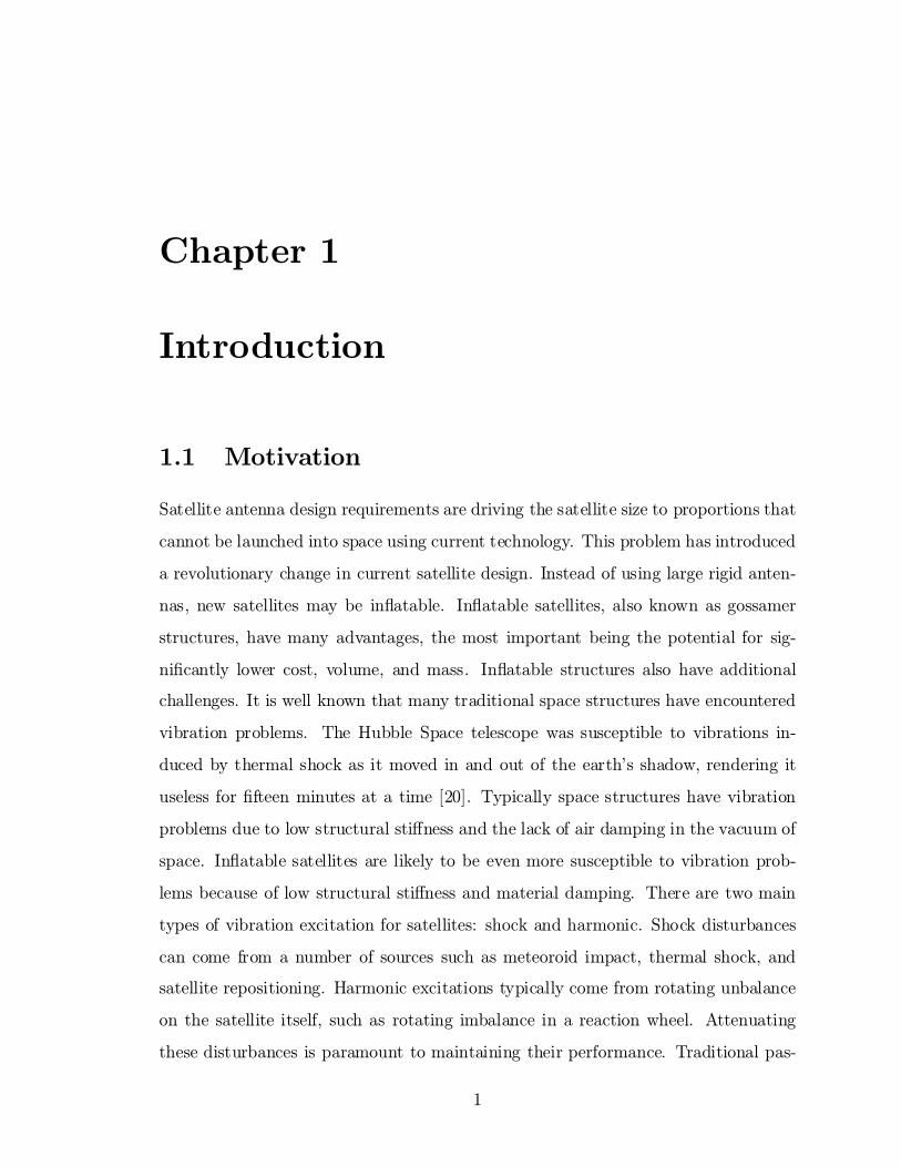
Experiment (IAE) shown in Figure 1.1 which was performed in 1996 [21]. L'Garde
and NASA JPL worked together to perform the experiment. Antennas of this type
could be used for space and mobile communications, earth observations, astronomical
observations, and space-based radar.
The satellite is made up of four major components: lens, torus, struts, and
2
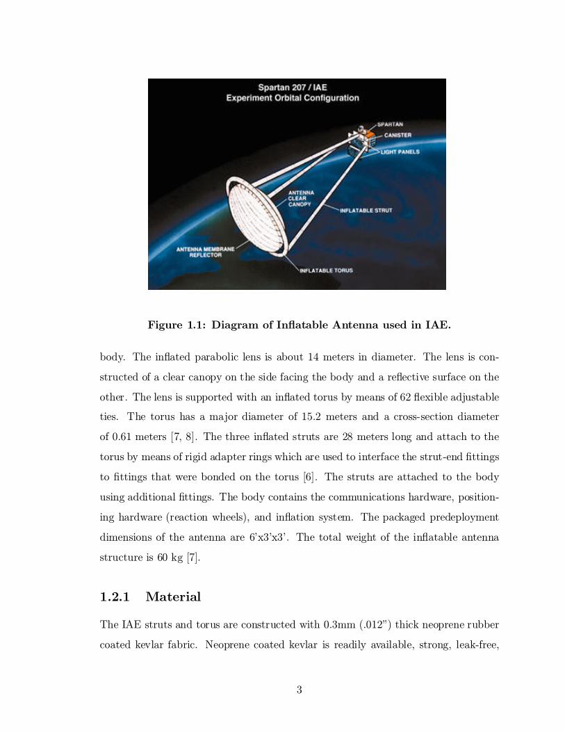
Figure 1.1: Diagram of In°atable Antenna used in IAE.
body. The in°ated parabolic lens is about 14 meters in diameter. The lens is con-
structed of a clear canopy on the side facing the body and a re°ective surface on the
other. The lens is supported with an in°ated torus by means of 62 °exible adjustable
ties. The torus has a major diameter of 15.2 meters and a cross-section diameter
of 0.61 meters [7, 8]. The three in°ated struts are 28 meters long and attach to the
torus by means of rigid adapter rings which are used to interface the strut-end ¯ttings
to ¯ttings that were bonded on the torus [6]. The struts are attached to the body
using additional ¯ttings. The body contains the communications hardware, position-
ing hardware (reaction wheels), and in°ation system. The packaged predeployment
dimensions of the antenna are 6'x3'x3'. The total weight of the in°atable antenna
structure is 60 kg [7].
1.2.1 Material
The IAE struts and torus are constructed with 0.3mm (.012") thick neoprene rubber
coated kevlar fabric. Neoprene coated kevlar is readily available, strong, leak-free,
3

bondable, °exible, and reasonably priced [7]. The material was selected because
L'Garde, the antenna manufacturer, had extensive experience using the material for
other projects.
The re°ector is made of 6.35 micron (0.00025") Mylar ¯lm with vapor deposited
aluminum to form the re°ective surface. The re°ector is fabricated by joining °at pie-
shaped gores, which are joined using Mylar tape. The canopy is made from the same
Mylar ¯lm without the addition of the re°ective coating. The re°ector is stressed,
via pressurization, to 6.89 MPa because this stress level has been shown to remove
the packaging wrinkles [8].
The analysis used in this paper will be based on the material Kapton, a thin
polyimide lm made by DuPont. The thickness of Kapton for this analysis is 0.003".
Kapton is a material that shows signi¯cant future promise for application in in°atable
space applications. It is stable at both high and low temperature extremes and is
tough and abrasion resistant. The analytical disadvantage of Kapton is that it exhibits
signi¯cant non-linear properties, being both temperature and frequency dependent.
1.2.2 Pressurization and Deployment
The IAE satellite structure, torus and struts, are in°ated with nitrogen to an operat-
ing pressure of about 2.9 psi. The lens is operated at a pressure of 0.29e-3 psi, much
lower than the rest of the structure [7]. Using the material Kapton, for the structure
but not the lens, the satellite structure would be pressurized to 0.5 psi, not to exceed
1 psi [23]. These pressurization levels, of about 0.5 psi, will be used in the following
analysis. The in°ation pressure is maintained by an on-board control system and
bottle of pressurized nitrogen. As the satellite moves in and out of the sun, nitrogen
may be vented and re¯lled to account for the change in pressure [23].
Deployment control is important for in°atable antennas to avoid damaging
them. The deployment sequence planned for the IAE was not successful due to
the presence of residual gas in the structure, which deployed it in an unanticipated
manner. Fortunately the antenna did deploy successfully, but in an uncontrolled
sequence. More development of ascent venting and deployment techniques is required
4

for future missions [6].
1.2.3 Ridigizable Structures
The satellites described here need to maintain their internal pressure to have struc-
tural sti®ness. Although, as mentioned above, the risk of meteroids and other objects
impacting the structures is relatively small, it may be desirable to have structures that
are ridigizable. These structures would deploy like the in°atables described above,
but would then ridigize so they no longer needed internal pressurization to maintain
their shape. Di®erent ridigization techniques are being examined, one of the most
prevalent being curing the material with ultraviolet light. The UV radiation in space
can be very intense and is an excellent source of energy for rigidizing a structure.
Other possibilities are thermoset materials, which could require a large amount of
thermal energy to cure, or water-based materials that harden as they dry [4].
1.3 Literary Review
1.3.1 Modeling and Test
A torus, although a fairly simple structure in concept, is actually numerically very
challenging. Few fully analytical solutions for the vibrations of toroids exist due to the
complexity of the problem. Numerical solutions for the axisymmetric vibrations of
toroids were examined in the 1960's by A. A. Liepins and P. F. Jordan [16, 17, 18, 13,
14]. Liepins uses ¯nite di®erence methods and Sanders linear shell theory to explore
the free vibrations of the prestressed toroidal shell [17]. Liepins is most concerned
with axisymmetric cross-sectional deformation of the torus, the deformation of the
tube, but also discusses in limited detail the global deformation of the torus, the ring
modes. The ring modes are approximated by the vibrations of a thin ring without
prestress. The relative importance of the types of mode depend on the torus aspect
ratio, de¯ned here as the radius of the tube divided by the radius of the ring as shown
in Figure 1.2.
5

Figure 1.2: De¯nition of Torus Dimensions.
Liepins also created numerical models of toroidal shells with non-constant wall
thicknesses and various types of support located at the inner and outer circumferences
of the torus [18]. A test was also performed by Jordan on toroids similar to those
modeled by Liepins [13]. Jordan found that the fundamental modes of the struc-
ture agreed well with predictions obtained from static asymptotic analysis using the
Rayleigh quotient. Interestingly he found signi¯cant acoustic structural interactions.
He proved the existence of the interactions by replacing part of the air in the test
object with helium.
Williams analytically investigated the modes of a tensioned membrane [24].
He then examined the e®ect on the modes with a piezopolymer patch attached to the
membrane. He found that adding the piezoelectric patch to the membrane reduced
the frequency slightly but did not appreciably change the mode shapes. He also
found that the distribution of mass on the patch was signi¯cant, for instance a thin
large patch of the same mass as a thick small patch produced a di®erent result. The
mass that was more concentrated in the center of the patch, the thick small patch,
lowered the frequency more than the more dispersed mass. His ¯nal conclusion was
6
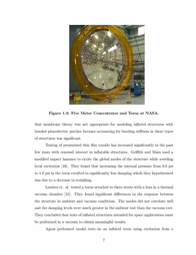
Figure 1.3: Five Meter Concentrator and Torus at NASA.
that membrane theory was not appropriate for modeling in°ated structures with
bonded piezoelectric patches because accounting for bending sti®ness in these types
of structures was signi¯cant.
Testing of pressurized thin lm toroids has increased signi¯cantly in the past
few years with renewed interest in in°atable structures. Gri±th and Main used a
modi¯ed impact hammer to excite the global modes of the structure while avoiding
local excitation [10]. They found that increasing the internal pressure from 0.8 psi
to 1.0 psi in the torus resulted in signi¯cantly less damping which they hypothesized
was due to a decrease in wrinkling.
Lassiter et. al. tested a torus attached to three struts with a lens in a thermal
vacuum chamber [15]. They found signi¯cant di®erences in the response between
the structure in ambient and vacuum conditions. The modes did not correlate well
and the damping levels were much greater in the ambient test than the vacuum test.
They concluded that tests of in°ated structures intended for space applications must
be performed in a vacuum to obtain meaningful results.
Agnes performed modal tests on an in°ated torus using excitation from a
7

shaker and a piezoelectric patch. They were unable to clearly identify modes from the
test but did demonstrate the viability of piezoelectric excitation of the structure [1].
The torus was found to exhibit signi¯cant non-linear behavior and the damping was
extremely high. The PVDF excitation produced less interference with suspension
modes of the free-free torus than excitation from the shaker.
NASA has tested a 5 meter lens, torus, and strut assembly, shown in Fig-
ure 1.3. This testing is still ongoing but they have arrived at a number of signi¯cant
conclusions. A shaker can mass load the test article even if it is attached at a point
on a non-in°ated part. The physical properties of the structure can change over time,
particularly the sti®ness of the joints. It is possible to disassemble and reassemble an
in°ated structure and still have the same dynamic response. This information was
received directly from John Lassiter at NASA, the work will be presented at the SDM
conference in 2001.
Testing of in°ated structures, speci¯cally toroids, is still ongoing. Testing of
these structures has proved to be challenging and development of testing procedures
is still progressing.
1.3.2 Piezoelectric E®ect
The Curie brothers originally discovered piezoelectric materials in 1880 [22]. Piezo-
electric materials exhibit two useful properties: the direct and converse piezoelectric
e®ects. The direct piezoelectric e®ect produces a voltage in a material when it is
strained, acting as a sensor. The converse piezoelectric e®ect produces a strain in a
material when subjected to a voltage, acting as an actuator. Structures using piezo-
electric materials as both sensors and actuators are referred to as \Smart or Intelligent
Structures" because of their ability to \sense" and \repair" their condition through
control algorithms [22]. As structural requirements become more stringent many en-
gineers are turning to piezoelectric materials to help meet their design requirements.
The linear piezoelectric constitutive equations are written as
8

E = ¯SD¡ hS (1.1)
T = cDS ¡ htD (1.2)
and
D = ²TE + dT (1.3)
S = SET + dtE (1.4)
where T, E, S, and D are the vectors of stress, electric ¯eld, strain, and electric
displacement (charge per unit area), respectively, cD is the elasticity matrix at con-
stant dielectric displacement, h and d are the piezoelectric constant matrices, ¯S is
the dielectric impermeability matrix at constant strain, sE is the elastic compliance
matrix at constant electric ¯eld, ²T is the dielectric matrix at constant strain, and
the superscript t denotes the transpose of a matrix. The electrical and mechani-
cal forces are assumed to balance at all times (quasi-static approximation) to derive
equations (1.1), (1.2), (1.3), and (1.4). Equations (1.1) and (1.3) describe the direct
piezoelectric e®ect and equations (1.2) and (1.4) describe the converse piezoelectric
e®ect [22].
A simple way to think of the coupling between the piezo and base structure
is shown in Figure 1.4. For a given voltage and sti®ness ratio, ks=ka, the piezo will
output a known force and displacement. The slope of the constant voltage line is de-
termined by the piezoelectric properties of the material. In this 1-D model, the piezo,
with sti®ness ka is pushing against a spring of sti®ness ks. Under a constant voltage,
if the spring is very sti®, the piezo will output a large force, but little displacement,
if the spring is soft, the piezo will output a smaller force but larger displacement.
Piezoelectric devices can be subdivided into two main categories, piezoceramics
and piezopolymers. Piezoceramics, such as lead zirconate titanate (PZT) are sti® and
brittle materials, whereas piezopolymers, such as polyvinylidene °uoride (PVDF), are
highly °exible and tough materials. Piezoceramics generally have a higher electro-
9

∆x
Fa
s
kk
Constant Voltage Line
ks= 0
ks= ∞
PZTka
ks
∆x
Figure 1.4: 1-D Model of Force Output from a Piezoelectric Device.
mechanical coupling than piezopolymers so essentially they produce higher voltages
per strain and higher strains per voltage.
The piezoelectric e®ect occurs naturally in quartz crystals, but can be created
in other materials. For PVDF, piezoelectricity is induced in the material by stretching
the strip and applying a high voltage [22]. The direction of the voltage potential
across the strip determines the poling direction of the resulting piezoelectric device.
Other materials, such as PZT, require heating to their \Curie Temperature" and then
having a voltage applied to them to activate their piezoelectric properties and set the
poling direction. The poling direction determines the direction of deformation of the
material given the direction of voltage potential.
Dosch et. al. developed a method which allows a single piece of piezoelectric
material to simultaneously sense and actuate in a closed loop system. This allows
for truly collocated sensors and actuators [5]. The method is realized by using an
electrical bridge circuit to measure strain or time rate of strain in the actuator.
The pin-force model is one of the earliest and simplest models to describe the
force transferred from an actuator to a substrate. This model treats the actuator
10

and substrate as separate bodies connected by pins at the ends of the actuator. The
simple pin-force model allows the actuator to expand thereby bending the substrate.
It does not account for the bending sti®ness of the actuator. This model can be
inaccurate when the bending sti®ness of the actuator is not signi¯cantly less than
that of the substrate.
The Bernoulli-Euler model accounts for the bending sti®ness of both the actu-
ator and the substrate. Chaudhry and Rogers [3], using \Mechanics Considerations"
arrived at the Bernoulli-Euler model from a more \physical" derivation than previ-
ous solutions. Their new approach to the model arrived at the same mathematical
behavior as the more complicated Bernoulli-Euler model.
1.3.3 Control Design
Modern control theory came to the United States from Russia in 1957 after the ¯rst
launch of Sputnik. The Russians initially developed state space methods and pole
placement control techniques, while US engineers were using transfer functions to
describe dynamic systems [9]. For a controllable system, using state space methods,
it is possible to place the closed loop poles anywhere in the s-plane that the designer
desires, if all the states are measured. This means that the closed loop performance
can be speci¯ed to be anything that the designer wants. The problem with this
method is that it is usually not practical to measure all of the states of a system.
Using an observer, or state estimator, all of the states do not need to be measured.
One disadvantage of a state estimator is that it adds additional dynamics to the
system, essentially doubling the number of states.
The largest problem with observers in distributed structural dynamic systems
is the concept of observation spillover. A distributed system has an in¯nite number of
modes, however the designer usually only considers some small subset of the modes,
usually with the lowest natural frequencies. Observation spillover is the result of the
physical measurement of the unmodeled modes. The problem observation spillover
can cause instability in the unmodeled modes of the structure. For this reason it is
sometimes desirable not to estimate the states. One way to avoid observation spillover
11

is to directly use the output of the sensors for feedback control [19].
If the sensors and actuators are collocated the output of the sensor can be
fed back directly to the actuator. This method does not allow the designer to place
the poles arbitrarily but is simpler than state feedback. Direct output feedback has
in¯nite bandwidth so the e®ect of the controller on even the high frequency modes
can be very signi¯cant.
1.4 Overview of Thesis
1.4.1 Contribution
This thesis investigates the feasibility of using PVDF to attenuate vibration in an
in°ated torus. The purpose is to develop a predictive model that can be compared
with experimental results and will be useful in design. This predictive model is then
used to perform an initial study regarding the vibration control of an in°ated torus.
In addition, the e®ect of various in°ation pressures and aspect ratios on the vibration
of the torus is explored.
1.4.2 Approach
Chapter 2 describes the modeling approach for the torus. A commercial ¯nite element
package, ANSYS, is used to form the mass and sti®ness matrices of the pressurized
torus. The matrices are then reduced in MATLAB using mass condensation. The
eigenvalue problem is then solved for the reduced mass and sti®ness matrices and
subset of the modes are used to solve for the impulse response of the structure in a
state space formulation. Chapter 3 describes the modeling of the interaction between
the piezoelectric devices and the torus. Euler-Bernoulli beam theory is used to ap-
proximate the behavior of the PVDF bonded to the torus. An observer-based modal
state space controller and direct output velocity feedback controller are used to at-
tenuate vibration in the structure. Chapter 4 discusses the e®ect of torus aspect ratio
and pressure on the vibration of the torus. The passive e®ect of PVDF, considering
12

only its mass and sti®ness, on the torus is also examined. The e®ectiveness of each
controller is determined by considering the closed loop response of the system to an
impulse excitation.
13

Chapter 2
Modeling of a Torus
2.1 Introduction
Analytical solutions for the mode shapes and natural frequencies of a prestressed torus
are quite complex. The ¯nite element method provides a relatively easy way to model
the system. Commercial ¯nite element programs have become highly developed in the
past few years and their utility has increased with the development of faster and faster
computers. The analysis method presented here makes use of the availability of highly
re¯ned commercial ¯nite element programs to formulate mass and sti®ness matrices
representing the model. These mass and sti®ness matrices can then be manipulated
outside of the bounds of the ¯nite element package using MATLAB , a computer
mathematical tool specializing in matrix manipulation. The matrices extracted from
the ¯nite element model are large and need to be reduced for e±cient computation.
Mass condensation is performed before solving the eigenvalue problem and modal
truncation is used when designing the controller. The model is represented in state
space so that traditional control tools can be used to manipulate it. The MATLAB
code to perform this analysis can be found in the Appendix.
14
2.2 Finite Element Modeling
The torus was modeled in ANSYS using linear thin shell elements. Shell93 elements
were used that have 8 nodes, four corner nodes and four midside nodes. Each node
has 6 degrees of freedom, translation and rotation in x, y, and z. The rotational
inertia is assumed to be negligible for these elements so the rotational mass is zero.
The stress ¯eld in the pressurized torus is very sensitive to irregularities in the mesh,
therefore the mesh was created externally to ANSYS and then the node and element
de¯nitions were read in using input ¯les. The MATLAB code to generate the node
and element de¯nitions can be found in the Appendix. The model is de¯ned by the
geometry, based on the nodes and elements, the real constants, which de¯ne the shell
element thickness, and the material properties. These values are listed in Table 2.1.
The torus is made of Kapton and PVDF patches are attached to it to use as actuators
to implement the control algorithms.
Table 2.1: Finite Element Model Material Properties
Parameter SI EnglishKapton Elastic Modulus 2.55e9 Pa 0.370e6 psiKapton Mass Density 1418 kg/m3 1.328e-4 lb*s2/in4
Kapton Poisson's Ratio 0.34 0.34Kapton Thickness 76.2 ¹m 0.0030 inPVDF Elastic Modulus 3.0e9 Pa 0.435e6 psiPVDF Mass Density 1728 kg/m3 1.664e-4 lb*s2/in4
PVDF Poisson's Ratio 0.33 0.33PVDF Thickness 28.0 ¹m 0.0011 in
Table 2.2: Finite Element Model Geometric Properties
Parameter SI EnglishRing Diameter 15.24 m 600 inTube Diameter 0.61 m 24 in
15

PVDF Top Surface
PVDF Top Surface
PVDF Outer Surface
Front, PVDF Only
Front, PVDF & Kapton
PVDF Outer Surface
PVDFKapton
IsometricPVDF & Kapton
x
y
x
y
Figure 2.1: Locations of PVDF on Torus.
The PVDF patches were placed on the torus by collocating additional Shell93
elements on top of the existing elements. The location of these patches is shown
in Figure 2.1. This is an approximation of the actual structure because the two
elements exist in the same plane, thereby having a slightly lower bending sti®ness
than the actual structure.
An internal pressure of 0.5 psi was applied on all of the Kapton elements to
simulate the pressure in torus. The torus was restrained to zero displacement at one
node in all degrees of freedom to prevent rigid body motion and a static analysis was
performed using the option pstres,on to create a prestressed sti®ness matrix to be
used in the modal analysis to follow.
16

Before performing the modal analysis, the boundary conditions had to be
changed. The displacement constraint was removed to solve for the free-free response
of the torus. It was not necessary to remove the internal pressure because ANSYS
neglects any applied forces in a modal analysis. It should be noted that some of the
solution options were modi¯ed for better convergence. The subspace working size
(subsiz), number of extra vectors (npad ), and number of modes per memory block
(nperbk) were all doubled from their default values for better convergence. This
seemed to be necessary due to the ¯rst six frequencies being zero, the rigid body
modes, and the fact that most of the modes came in orthogonal pairs at the same
frequency.
2.2.1 Mass and Sti®ness Extraction
The information de¯ning the mass and sti®ness matrices is de¯ned in the ¯le job-
name.full created by ANSYS after performing a modal analysis. This le contains
the information in binary format that needs to be converted and extracted from the
¯le. This procedure is described in the Guide to Interfacing with ANSYS. It
should be noted for anyone who is interested in doing this that the process is not
trivial. It requires the user to have both the Microsoft Visual C++ compiler and the
Compaq Visual Fortran compiler of the speci¯c version referenced in the ANSYS
Installation and Con¯guration Guide. To compile the source code rdfull.f which
reads the mass and sti®ness matrices the user ¯rst needs to rename the source code
rdfull.f to userprog.f. The user then needs to run the ANSYS program rdrwrt.bat with
the option userprog from a DOS window, the full command is rdrwrt userprog. This
produces the executable userprog.exe which is used to extract the mass and sti®ness
matrices from the ¯le jobname.full by renaming the le jobname.full to ¯le.full and
then executing userprog.exe in the directory where ¯le.full resides. It should be noted
that the author never got this procedure to fully work under Windows98, he could
never compile the source code userprog.f. The author believes the root of the problem
to be that the Windows98 environment seems to have problems setting environment
variables from batch ¯les. He has been assured that the procedure does work on a
17

WindowsNT platform. Eventually he got a compiled version of the le userprog.exe
from the ANSYS support representative and just used that. However, to run that
¯le the user still needs to have the Compaq Visual Fortran compiler installed on the
computer system.
The output from running the program userprog.exe in the same directory as
the ¯le le.full is two ¯les, MASS.MATRIX and STIFFNESS.MATRIX. These ¯les
consist of three columns of numbers representing the row number, column number,
and nonzero value of the matrix entry. They only contain the upper diagonal portion
of the matrix. The model degrees of freedom are ordered by node number and nodal
degree of freedom. For instance, for a two node model with six degrees of freedom
per node, the model degrees of freedom are represented by
x =
26666666666666666666666666666664
x1
y1
z1
rotx1
roty1
rotz1
x2
y2
z2
rotx2
roty2
rotz2
37777777777777777777777777777775
(2.1)
2.3 Finite Element Model Veri¯cation
A number of test cases are examined to verify the use of the commercial ¯nite element
program ANSYS to model the dynamics of prestressed structures. First a tensioned
string and tensioned membrane are compared to analytical solutions. Then conver-
gence is demonstrated on the model of the torus by solving for the modal frequencies
18
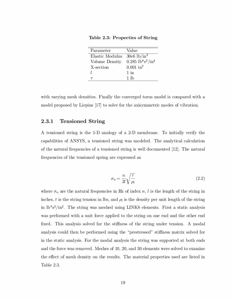
Table 2.3: Properties of String
Parameter ValueElastic Modulus 30e6 lb/in2
Volume Density 0.285 lb*s2/in4
X-section 0.001 in2
l 1 in¿ 1 lb
with varying mesh densities. Finally the converged torus model is compared with a
model proposed by Liepins [17] to solve for the axisymmetric modes of vibration.
2.3.1 Tensioned String
A tensioned string is the 1-D analogy of a 2-D membrane. To initially verify the
capabilities of ANSYS, a tensioned string was modeled. The analytical calculation
of the natural frequencies of a tensioned string is well documented [12]. The natural
frequencies of the tensioned spring are expressed as
¾n =n
2l
r¿
½l(2.2)
where ¾n are the natural frequencies in Hz of index n, l is the length of the string in
inches, t is the string tension in lbs, and ½l is the density per unit length of the string
in lb*s2/in2. The string was meshed using LINK8 elements. First a static analysis
was performed with a unit force applied to the string on one end and the other end
¯xed. This analysis solved for the sti®ness of the string under tension. A modal
analysis could then be performed using the \prestressed" sti®ness matrix solved for
in the static analysis. For the modal analysis the string was supported at both ends
and the force was removed. Meshes of 10, 20, and 30 elements were solved to examine
the e®ect of mesh density on the results. The material properties used are listed in
Table 2.3.
19
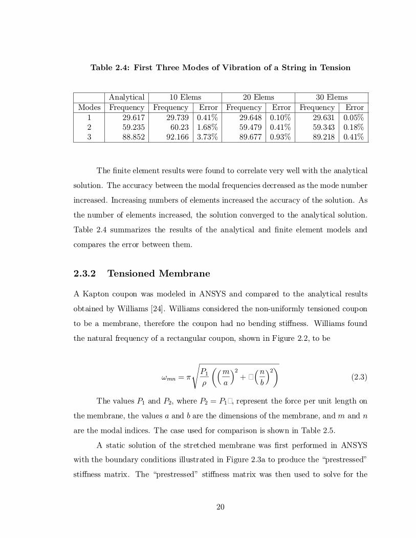
Table 2.4: First Three Modes of Vibration of a String in Tension
Analytical 10 Elems 20 Elems 30 ElemsModes Frequency Frequency Error Frequency Error Frequency Error
1 29.617 29.739 0.41% 29.648 0.10% 29.631 0.05%2 59.235 60.23 1.68% 59.479 0.41% 59.343 0.18%3 88.852 92.166 3.73% 89.677 0.93% 89.218 0.41%
The ¯nite element results were found to correlate very well with the analytical
solution. The accuracy between the modal frequencies decreased as the mode number
increased. Increasing numbers of elements increased the accuracy of the solution. As
the number of elements increased, the solution converged to the analytical solution.
Table 2.4 summarizes the results of the analytical and ¯nite element models and
compares the error between them.
2.3.2 Tensioned Membrane
A Kapton coupon was modeled in ANSYS and compared to the analytical results
obtained by Williams [24]. Williams considered the non-uniformly tensioned coupon
to be a membrane, therefore the coupon had no bending sti®ness. Williams found
the natural frequency of a rectangular coupon, shown in Figure 2.2, to be
!mn = ¼
sP1
½
µ³ma
´2
+ ·³nb
´2
(2.3)
The values P1 and P2, where P2 = P1·, represent the force per unit length on
the membrane, the values a and b are the dimensions of the membrane, and m and n
are the modal indices. The case used for comparison is shown in Table 2.5.
A static solution of the stretched membrane was ¯rst performed in ANSYS
with the boundary conditions illustrated in Figure 2.3a to produce the \prestressed"
sti®ness matrix. The \prestressed" sti®ness matrix was then used to solve for the
20

a
b
P1
P2=κP1
y
x
Figure 2.2: Membrane Coupon Under Non-Uniform Tension P1 and P2
Table 2.5: Properties of Membrane
Parameter ValueP1 0.75 lb/in· 2½ 3.98e-7 lb s/in3
a 5.0 inb 2.5 inE 0.37e6 lb/in2
21

y
x
P2=P1*κ
P1
Fixed y and z
Fixed x and z
Fixed x, y and z
Fixed x, y and z
Fixed x, y andz
Fixed x, y and z
(a) (b)
Figure 2.3: (a) Boundary Conditions for Static Analysis(b) Boundary Conditions for Dynamic Analysis
¯rst 20 modes of the structure. The boundary conditions used for the modal analysis
are shown in Figure 2.3b.
The analytical and ¯nite element models agreed very well. The error was less
than one percent for the ¯rst 19 modes. The analytical and ¯nite element calculations
of natural frequency, and the error between them, are shown in Table 2.6.
It is interesting to note that the error was related not to the frequency but to
the highest modal index. For instance, the 4,2 mode had a lower error than the 6,1
mode even though the 4,2 mode had a higher frequency. This is expected because
the larger number of elements in the long dimension could more accurately represent
the curvature of the membrane at higher order modes in the long dimension than the
smaller number of elements in the short dimension. This allowed for a more accurate
result of higher order modes in the long dimension than the short. For instance the
error in the m=3, n=1 mode is much less than the m=1, n=3 mode.
22

Table 2.6: Analytical and Finite Element Natural Frequencies of TensionedMembrane.
Analytical Finite ElementModes m n wmn fmn, Hz f, Hz Error
1 1 1 2586.58 411.67 412.07 0.098%2 2 1 2986.73 475.35 475.84 0.102%3 3 1 3554.92 565.78 566.62 0.148%4 4 1 4223.87 672.25 673.83 0.235%5 5 1 4952.93 788.28 790.6 0.294%6 1 2 4952.93 788.28 791.17 0.366%7 2 2 5173.17 823.34 825.63 0.279%8 3 2 5520.74 878.65 881.08 0.276%9 6 1 5719.15 910.23 915.1 0.535%10 4 2 5973.46 950.71 953.57 0.301%11 5 2 6509.43 1036.01 1039.8 0.366%12 7 1 6509.43 1036.01 1043.7 0.743%13 6 2 7109.84 1131.57 1137 0.480%14 8 1 7315.96 1164.37 1175.8 0.981%15 1 3 7366.59 1172.43 1179.7 0.620%16 2 3 7516.44 1196.28 1203.54 0.607%17 3 3 7759.75 1235.00 1242.2 0.583%18 7 2 7759.75 1235.00 1242.8 0.631%19 4 3 8088.10 1287.26 1294.6 0.570%20 9 1 8133.93 1294.55 1310.9 1.263%
23
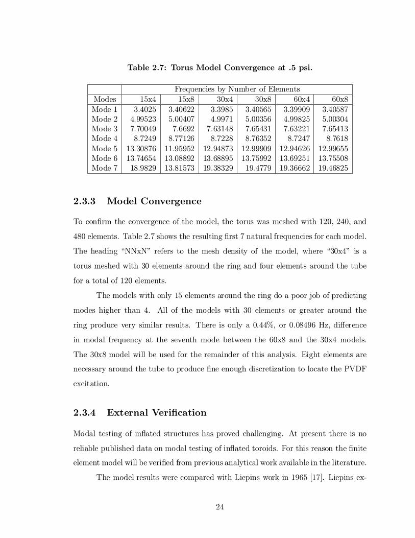
Table 2.7: Torus Model Convergence at .5 psi.
Frequencies by Number of ElementsModes 15x4 15x8 30x4 30x8 60x4 60x8Mode 1 3.4025 3.40622 3.3985 3.40565 3.39909 3.40587Mode 2 4.99523 5.00407 4.9971 5.00356 4.99825 5.00304Mode 3 7.70049 7.6692 7.63148 7.65431 7.63221 7.65413Mode 4 8.7249 8.77126 8.7228 8.76352 8.7247 8.7618Mode 5 13.30876 11.95952 12.94873 12.99909 12.94626 12.99655Mode 6 13.74654 13.08892 13.68895 13.75992 13.69251 13.75508Mode 7 18.9829 13.81573 19.38329 19.4779 19.36662 19.46825
2.3.3 Model Convergence
To con¯rm the convergence of the model, the torus was meshed with 120, 240, and
480 elements. Table 2.7 shows the resulting ¯rst 7 natural frequencies for each model.
The heading \NNxN" refers to the mesh density of the model, where \30x4" is a
torus meshed with 30 elements around the ring and four elements around the tube
for a total of 120 elements.
The models with only 15 elements around the ring do a poor job of predicting
modes higher than 4. All of the models with 30 elements or greater around the
ring produce very similar results. There is only a 0.44%, or 0.08496 Hz, di®erence
in modal frequency at the seventh mode between the 60x8 and the 30x4 models.
The 30x8 model will be used for the remainder of this analysis. Eight elements are
necessary around the tube to produce ¯ne enough discretization to locate the PVDF
excitation.
2.3.4 External Veri¯cation
Modal testing of in°ated structures has proved challenging. At present there is no
reliable published data on modal testing of in°ated toroids. For this reason the ¯nite
element model will be veri¯ed from previous analytical work available in the literature.
The model results were compared with Liepins work in 1965 [17]. Liepins ex-
24
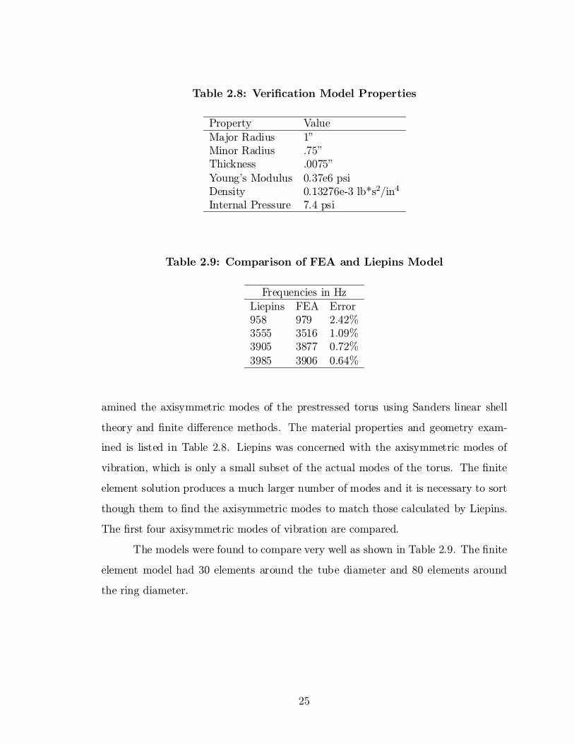
Table 2.8: Veri¯cation Model Properties
Property ValueMajor Radius 1"Minor Radius .75"Thickness .0075"Young's Modulus 0.37e6 psiDensity 0.13276e-3 lb*s2/in4
Internal Pressure 7.4 psi
Table 2.9: Comparison of FEA and Liepins Model
Frequencies in HzLiepins FEA Error958 979 2.42%3555 3516 1.09%3905 3877 0.72%3985 3906 0.64%
amined the axisymmetric modes of the prestressed torus using Sanders linear shell
theory and ¯nite di®erence methods. The material properties and geometry exam-
ined is listed in Table 2.8. Liepins was concerned with the axisymmetric modes of
vibration, which is only a small subset of the actual modes of the torus. The ¯nite
element solution produces a much larger number of modes and it is necessary to sort
though them to ¯nd the axisymmetric modes to match those calculated by Liepins.
The ¯rst four axisymmetric modes of vibration are compared.
The models were found to compare very well as shown in Table 2.9. The ¯nite
element model had 30 elements around the tube diameter and 80 elements around
the ring diameter.
25
2.4 Problem Formulation
The dynamics of the torus can be represented by Newton's second law, F = ma.
Summing forces on the torus results in the matrix equation
M Äx+Kx = f (2.4)
y = Cx (2.5)
where M and K represent the symmetric mass and sti®ness matrices, x and Äx are the
vectors of displacement and acceleration, and f is a vector of external disturbances.
The vector y is the desired output from the system. The mass and sti®ness matrices
are initially very large, on the order of 4000 by 4000, and can be condensed using
mass condensation. These matrices need to be reduced in order to solve the eigen-
value problem to determine the natural frequencies and modes of vibration. Without
reducing the number of degrees of freedom in the system, MATLAB was unable to
solve for the eigenvalues and eigenvectors. In addition, because the rotational inertia
of the shells is neglected, there are zeros on the diagonal of the mass matrix. These
massless degrees of freedom need to be removed for many solution techniques to work.
The MATLAB code used to perform the following modeling steps can be found in the
Appendix.
2.4.1 Mass Condensation
Mass condensation is essentially a speci¯c case of Guyan reduction where only mass-
less degrees of freedom are removed [12]. Guyan reduction is a common model reduc-
tion technique which is de¯ned in many texts, for example, Inman 1996. In this case
all of the rotational degrees of freedom are massless. The Shell93 elements used in the
¯nite element analysis assume that the rotational inertia is negligible in the model
and so the rotational masses are zero, therefore they can be removed. Mass con-
densation, or Guyan reduction, is characterized by separating the mass and sti®ness
matrices into signi¯cant and insigni¯cant degrees of freedom, x1 and x2 respectively.
This results in the matrix equation
26

24 M11 M12
M21 M22
3524 Äx1
Äx2
35 +
24 K11 K12
K21 K22
3524 x1
x2
35 =
24 f1
f2
35 (2.6)
The method of Guyan reduction leads to the coordinate transformation matrix Q.
This coordinate transformation reduces the full coordinate system x to the reduced
coordinates x1. The coordinate transformation is de¯ned by
x = Qx1 (2.7)
where
Q =
24 I
¡K¡122 K21
35 (2.8)
So if equation (2.6) is premultiplied by QT the reduced order system is represented
by
¹M Äx1 + ¹Kx1 = QTf (2.9)
where ¹M = QTMQ and ¹K = QTKQ. Now having a reduced order system the
eigenvalue problem can be performed to solve for the eigenvalues and eigenvectors of
the system.
2.4.2 Eigenvalue Solution
The eigenvalue problem is de¯ned such that for a matrix X, X© = ©¤, where
¤ is a diagonal matrix of eigenvalues and © is a matrix of eigenvectors. Choleski
decomposition is used to transform the equation of motion, equation (2.9) in this
case, to a symmetric eigenvalue problem. Choleski decomposition is de¯ned by the
equation
27
U TU = ¹M (2.10)
This equation leads us to the coordinate transformation de¯ned as
x1 = U¡1q (2.11)
Applying the coordinate transformation to equation (2.9) we get the following equa-
tions
UTU Äx1 + ¹Kx1 = QTf (2.12)
UT Äq + ¹KU¡1q = QTf (2.13)
Äq + U¡T ¹KU¡1 = U¡TQTf (2.14)
~K = U¡T ¹KU¡1 (2.15)
Solving the eigenvalue problem for ~K produces the matrices ¤ and ©, the eigenvalues
and eigenvectors respectively.
The eigenvalue problem was solved using the MATLAB eigs function. This
function allows the user to request the number and range of eigenvalues. In this
case it was desirable to get the ¯rst few lowest eigenvalues and their corresponding
eigenvectors. It should be recognized that this produces a non-square matrix of
eigenvectors. The eigenvectors have been transformed with two prior coordinate
transformations as de¯ned by equations (2.7) and (2.11). To obtain the physical mode
shapes it is necessary to reverse the coordinate transformations on the eigenvectors
by
¹ª = QU¡1© (2.16)
These physical mode shapes are not mass normalized due to the mass conden-
sation. The coordinate transformation U¡1© produces mass normalized transformed
28
mode shapes, but then the transformation back to physical coordinates from the
mass condensation coordinates removes the mass normalization. In other words if
the mass condensation had not been performed you would have the mass normalized
mode shapes at this point. The physical mode shapes are mass normalized by
¹ª = [¹ª1; ¹ª2; :::; ¹ªn] (2.17)
mi = ¹ªTiM ¹ªi (2.18)
ªi = 1pmi
¹ªi (2.19)
ª = [ª1;ª2; :::;ªn] (2.20)
2.4.3 Modal Equations
The equation of motion, equation (2.5), can now be expressed in modal coordinates,
through the modal transformation
x = ªr (2.21)
as
IÄr + ¤r = ªTf (2.22)
y = Cªr (2.23)
by recognizing that
ªTMª = I (2.24)
ªTKª = ¤ (2.25)
because the eigenvectors are mass normalized. The modal equation consists of square
matrices. The matrix ¤ is a diagonal matrix of natural frequency, in rad/s, squared.
The rigid body modes were removed from the mode shape matrix ª for a clearer
understanding of the behavior of the structure [12].
29
2.4.4 State Space Formulation
The modal equation was then reduced to ¯rst order by the transformation
q1 = r
q2 = _r(2.26)
yielding
24 _q1
_q2
35 =
24 0 1
¡¤ 0
3524 q1
q2
35+
24 0
ªTB
35 f (2.27)
y =hCª 0
iq (2.28)
where f is now a horizontal vector of n inputs and B is a matrix with n columns.
The product Bf is equivalent to the vector f used previously, as in equation (2.5).
Equation (2.27) considers no damping. Modal damping can be added in the
form 2³!n where !n is the modal frequency and ³ is the damping ratio. In this case
both !n and ³ are matrices. The matrix of modal frequencies can be expressed asp
¤ and the matrix of damping ratios is a diagonal matrix of the individual modal
damping ratios. A modal damping ratio of 0.01 will be used here. Therefore, adding
damping results in the equation
24 _q1
_q2
35 =
24 0 1
¡¤ ¡2³p
¤
3524 q1
q2
35+
24 0
ªTB
35 f (2.29)
Equations (2.29) and (2.28) can now be expressed in compact form as
_q = ¹Aq + ¹Bf (2.30)
y = ¹Cq (2.31)
Using this form a controller can now be designed.
30

2.5 Summary
At this point a state space model has been developed to describe the dynamics of
the free-free torus. This representation is in modal space and the response is based
upon the summation of a truncated set of the modes of vibration, indirectly the
eigenvectors, of the system. The modal frequencies are also solved, represented by
the square root of the eigenvalues. The MATLAB code is validated by comparing the
natural frequencies and mode shapes as calculated by MATLAB to those calculated
by ANSYS, they are found to match to a minimum of four decimal places. The next
chapter will derive a model for determining the force transferred to the torus by the
PVDF and will then examine two control methods for attenuating vibration in the
torus.
31

Chapter 3
Actuators and Control Design
3.1 Introduction
To attenuate vibration in the torus, a closed loop control design is implemented.
Piezoelectric patches, made of PVDF, are bonded to the surface of the torus and act
as both sensors and actuators. This chapter will discuss the modeling of the actuators
and the design of the control system. The bonded piezoelectric patches are treated
as layered beams to determine the force output to the torus. Two control techniques
are examined. Pole placement techniques are initially chosen as a one of the most
basic benchmark state space control techniques. Velocity feedback is examined as a
simpler control algorithm. Optimal control is brie°y discussed as a better alternative
for choosing gain matrices in multi-input systems. None of the controllers designed
here are likely ideal. The controllers chosen here are for the purpose of demonstrating
the controllability of the system, not necessarily because they are the best controllers
to use.
3.2 Piezoelectric Modeling
One of the simplest models of actuator-substrate interaction is the pin-force method.
This method treats the substrate as a beam and the actuator as an expanding rod
with their ends pinned. When the actuator expands it produces a moment on the
32
substrate thereby bending it. This model can be highly inaccurate because it does
not consider the bending sti®ness of the actuator. The Bernoulli-Euler model does
account for the bending sti®ness of the actuator.
To determine the force transferred to the torus from the piezoelectric patches,
Bernoulli-Euler beam theory is used. This method treats the actuator and substrate
as a composite beam. The strain at the interface between the actuator and substrate
is equal, using the assumption of perfect bonding. This assumption leads us to the
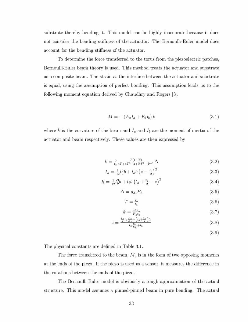
following moment equation derived by Chaudhry and Rogers [3].
M = ¡ (EaIa + EbIb) k (3.1)
where k is the curvature of the beam and Ia and Ib are the moment of inertia of the
actuator and beam respectively. These values are then expressed by
k = 6tb
T(1+T)6T+4T2+4+ªT2+ª¡1¢ (3.2)
Ia = 112t3ab+ tab
¡z ¡ ta
2
¢2(3.3)
Ib = 112t3bb + tbb
¡ta + tb
2¡ z¢2
(3.4)
¢ = d31E3 (3.5)
T = tbta
(3.6)
ª = EbtbEata
(3.7)
z =ta2 ta
EaEb
+(ta+tb2 )tb
taEaEb
+tb(3.8)
(3.9)
The physical constants are de¯ned in Table 3.1.
The force transferred to the beam, M , is in the form of two opposing moments
at the ends of the piezo. If the piezo is used as a sensor, it measures the di®erence in
the rotations between the ends of the piezo.
The Bernoulli-Euler model is obviously a rough approximation of the actual
structure. This model assumes a pinned-pinned beam in pure bending. The actual
33
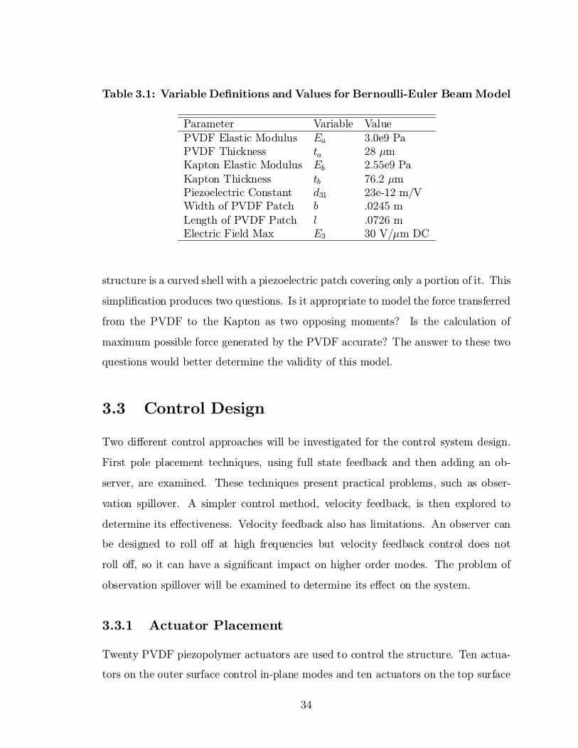
Table 3.1: Variable De¯nitions and Values for Bernoulli-Euler Beam Model
Parameter Variable ValuePVDF Elastic Modulus Ea 3.0e9 PaPVDF Thickness ta 28 ¹mKapton Elastic Modulus Eb 2.55e9 PaKapton Thickness tb 76.2 ¹mPiezoelectric Constant d31 23e-12 m/VWidth of PVDF Patch b .0245 mLength of PVDF Patch l .0726 mElectric Field Max E3 30 V/¹m DC
structure is a curved shell with a piezoelectric patch covering only a portion of it. This
simpli¯cation produces two questions. Is it appropriate to model the force transferred
from the PVDF to the Kapton as two opposing moments? Is the calculation of
maximum possible force generated by the PVDF accurate? The answer to these two
questions would better determine the validity of this model.
3.3 Control Design
Two di®erent control approaches will be investigated for the control system design.
First pole placement techniques, using full state feedback and then adding an ob-
server, are examined. These techniques present practical problems, such as obser-
vation spillover. A simpler control method, velocity feedback, is then explored to
determine its e®ectiveness. Velocity feedback also has limitations. An observer can
be designed to roll o® at high frequencies but velocity feedback control does not
roll o®, so it can have a signi¯cant impact on higher order modes. The problem of
observation spillover will be examined to determine its e®ect on the system.
3.3.1 Actuator Placement
Twenty PVDF piezopolymer actuators are used to control the structure. Ten actua-
tors on the outer surface control in-plane modes and ten actuators on the top surface
34

control out-of-plane modes. The location and number of these actuators has been
chosen somewhat arbitrarily. The piezos used as actuators are also used as sensors
on the model. This can be accomplished through the process developed by Dosch,
Inman, and Garcia [5]. Using this process produces collocated sensors and actuators.
The force from the actuator in°uences the system through the control input
matrix B in equation (2.29). For a system with twenty actuators B has dimensions
of 10x20, considering ten modes. The actuators are assumed to bend only on their
primary axis. The actuators on the outer surface create force in only the rotz (rotation
about the z axis) direction. The actuators on the top surface create force in both the
rotx and roty direction depending on their orientation. See Figure 2.1 for a de¯nition
of the coordinate system.
Consider the example of a four node system with rotations in x, y , and z at
each node. The ¯rst two nodes represent a piezo on the top of the torus and the
second two nodes represent a piezo on the bottom of the torus. The angle µ is the
angle from the x axis, in the xy-plane to the center of the piezo. For this case the
control input matrix B is
B =
26666666666666666666666666666664
1 0
0 0
0 0
¡1 0
0 0
0 0
0 Cos(µ)
0 Sin(µ)
0 0
0 ¡Cos(µ)0 ¡Sin(µ)0 0
37777777777777777777777777777775
(3.10)
where the states are
35
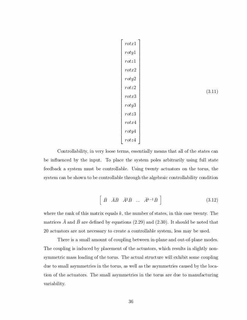
26666666666666666666666666666664
rotx1
roty1
rotz1
rotx2
roty2
rotz2
rotx3
roty3
rotz3
rotx4
roty4
rotz4
37777777777777777777777777777775
(3.11)
Controllability, in very loose terms, essentially means that all of the states can
be in°uenced by the input. To place the system poles arbitrarily using full state
feedback a system must be controllable. Using twenty actuators on the torus, the
system can be shown to be controllable through the algebraic controllability condition
h¹B ¹A ¹B ¹A2 ¹B ::: ¹Ak¡1 ¹B
i(3.12)
where the rank of this matrix equals k, the number of states, in this case twenty. The
matrices ¹A and ¹B are de¯ned by equations (2.29) and (2.30). It should be noted that
20 actuators are not necessary to create a controllable system, less may be used.
There is a small amount of coupling between in-plane and out-of-plane modes.
The coupling is induced by placement of the actuators, which results in slightly non-
symmetric mass loading of the torus. The actual structure will exhibit some coupling
due to small asymmetries in the torus, as well as the asymmetries caused by the loca-
tion of the actuators. The small asymmetries in the torus are due to manufacturing
variability.
36
0 5 1 0 1 5- 0 . 0 5
- 0 . 0 4
- 0 . 0 3
- 0 . 0 2
- 0 . 0 1
0
0 . 0 1
0 . 0 2
0 . 0 3
0 . 0 4
T i m e , s
Res
pons
e, m
icro
ns
S e t t l e T i m e : I n P l a n e 1 2 . 1 8 s , O u t o f P l a n e 9 . 3 0 s
I n P l a n e M o t i o n O u t o f P l a n e M o t i o n
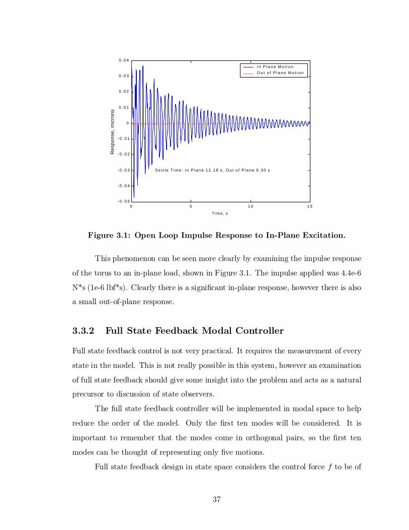
Figure 3.1: Open Loop Impulse Response to In-Plane Excitation.
This phenomenon can be seen more clearly by examining the impulse response
of the torus to an in-plane load, shown in Figure 3.1. The impulse applied was 4.4e-6
N*s (1e-6 lbf*s). Clearly there is a signi¯cant in-plane response, however there is also
a small out-of-plane response.
3.3.2 Full State Feedback Modal Controller
Full state feedback control is not very practical. It requires the measurement of every
state in the model. This is not really possible in this system, however an examination
of full state feedback should give some insight into the problem and acts as a natural
precursor to discussion of state observers.
The full state feedback controller will be implemented in modal space to help
reduce the order of the model. Only the ¯rst ten modes will be considered. It is
important to remember that the modes come in orthogonal pairs, so the ¯rst ten
modes can be thought of representing only ¯ve motions.
Full state feedback design in state space considers the control force f to be of
37
the form
f = ¡Gq (3.13)
where G has as many rows as inputs. Substituting the result from equation (3.13)
into equation (2.30) produces
_q = ( ¹A ¡ ¹BG)q (3.14)
Physically this represents a controller that can measure every state in the model
and then using these measurements, feed back force to the actuators. This model is
not representative of the actual system because all of the states cannot be directly
measured. The only states that can be directly measured are those measured by the
piezos. The matrix B represents the location of the inputs to the system.
At this point the poles of ( ¹A ¡ ¹BG) can be chosen to be any value by the
appropriate choice of the G matrix. The limitation on the choice of the poles is that
the more the poles are moved the greater the values in the G matrix and thus the
greater the required actuator force.
Consider an external disturbance expressed as
24 _q1
_q2
35 =
24 0 1
¡¤ ¡2³p
¤
3524 q1
q2
35+
24 0
ªTB
35 f +
24 0
ªTF
35 fd (3.15)
where fd is the external disturbance and F is a pointer to show where the external
disturbance acts. Now equation (3.15) can be written in compact form as
_q = ( ¹A¡ ¹BG)q + ¹Ffd (3.16)
Using this equation the closed loop response of the system to an external disturbance
can be determined.
38
3.3.3 Observer-Based Feedback Design
It is not practical to measure all the states of a model, as noted in the discussion of
full state feedback. A more feasible approach to control design is to use an observer.
An observer estimates the states of the system by measuring only a subset of the
states, through the sensors in the system [9]. The estimated states, q, are then used
to implement feedback in the same manner as full state feedback. The key di®erence
is that the feedback is based on the estimated states, q, not the actual states, q. Thus
the control law is
f = ¡Gq (3.17)
The observer is represented by the equation
_q = ¹Aq + ¹Bf +K(ysens ¡ ¹Csensq) (3.18)
where K is a matrix of gains and ysens is the sensor output represented by
ysens = ¹Csensq (3.19)
Under the assumption that the sensor output, ysens represents both position and
velocity, ¹Csens can be expressed as
¹Csens = [Csensª Csensª] (3.20)
Consider the example of a four node system with rotations in x, y , and z at
each node. The ¯rst two nodes represent a piezo on the top of the torus and the
second two nodes represent a piezo on the bottom of the torus. The angle µ is the
angle from the x axis, in the xy-plane to the center of the piezo. Reference Figure 2.1
for a de¯nition of the coordinate system.
39
In this case there are two outputs making the vector ysens a 2x1. The matrix
Csens is then de¯ned as
Csens =
24 0 0 1 0 0 ¡1 0 0 0 0 0 0
0 0 0 0 0 0 Cos(µ) Sin(µ) 0 ¡Cos(µ) ¡Sin(µ) 0
35
(3.21)
where the states are
26666666666666666666666666666664
rotx1
roty1
rotz1
rotx2
roty2
rotz2
rotx3
roty3
rotz3
rotx4
roty4
rotz4
37777777777777777777777777777775
(3.22)
It is clear from equation (3.18) that the observer is a dynamic system. Thus
the estimated states have a dynamic response. The error between the estimated states
and the actual states is expressed by
_e = ( ¹A¡K ¹Csens)e (3.23)
The speed at which the error converges to zero depends on the location of the
poles of the matrix ¹A ¡K ¹Csens. These poles can be chosen to be any value through
40
the gain matrix K as long as the system is observable. Observability is the parallel
to controllability discussed above and is determined by ¯nding the rank of the matrix
h¹CTsens
¹AT ¹CTsens ( ¹AT )2 ¹CT
sens ::: ( ¹AT)k¡1 ¹CTsens
i(3.24)
If the rank is k, the number of states, then the system is observable [9].
The gain matrix, K, determines the poles of the observer and thus the dynamic
response of the observer. It is generally desirable to have the observer respond much
faster than the physical system. This is analogous to picking the gain matrix G
when designing a full state compensator, however there is one signi¯cant di®erence.
Choosing large gains G results in large control forces. The gains K are internal to
the system and do not manifest themselves in any physical actuation in the observer
system so there is no direct limitation on their value. It is, however, desirable to limit
the gains K because they a®ect the magnitude of the compensator. A compensator
with large magnitudes will have more sensitivity to noise.
The complete dynamic system, the physical system and the observer expressed
by equations (2.30) and (3.18), can now be combined to produce
24 _q
_q
35 =
24
¹A ¡ ¹BG
K ¹Csens ¹A¡K ¹Csens¡ ¹BG
3524 q
q
35+
24
¹F
0
35 fd (3.25)
The poles of this system can be shown to be equal to the poles of ¹A ¡ ¹BG and
¹A ¡ K ¹C [9]. This means that the poles of the complete dynamic system are the
combination of the poles that were chosen for full state feedback and the poles that
were chosen for the observer. Using this information the gain matrices G and K can
be chosen to fully de¯ne the response of the system.
The disadvantage of using an observer is that it adds additional dynamics
to the system. This can lead to the problem of observation spillover. Observation
spillover can produce instability in the system. Observers can be designed to roll o®
at higher frequencies in order to reduce the potential for instability. The spillover can
41
be reduced if the sensor signals are ltered to remove contributions of higher order
modes [19].
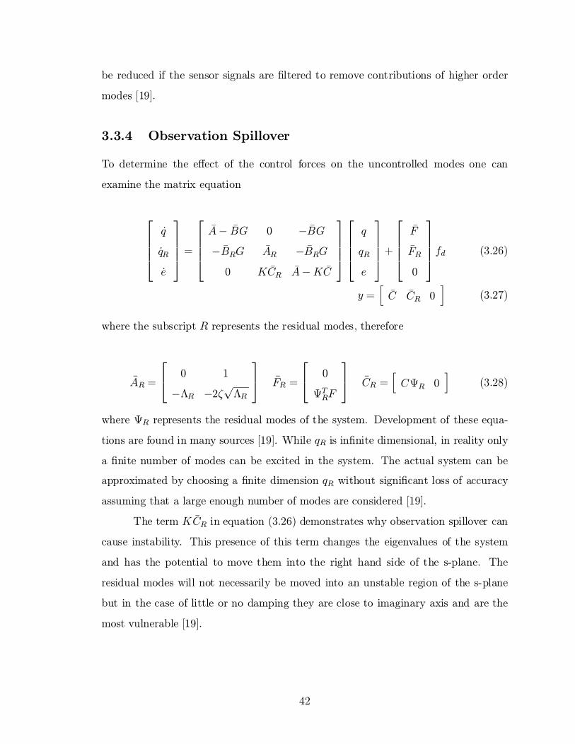
3.3.4 Observation Spillover
To determine the e®ect of the control forces on the uncontrolled modes one can
examine the matrix equation
26664
_q
_qR
_e
37775 =
26664
¹A¡ ¹BG 0 ¡ ¹BG
¡ ¹BRG ¹AR ¡ ¹BRG
0 K ¹CR ¹A¡K ¹C
37775
26664
q
qR
e
37775+
26664
¹F
¹FR
0
37775 fd (3.26)
y =h
¹C ¹CR 0i
(3.27)
where the subscript R represents the residual modes, therefore
¹AR =
24 0 1
¡¤R ¡2³p
¤R
35 ¹FR =
24 0
ªTRF
35 ¹CR =
hCªR 0
i(3.28)
where ªR represents the residual modes of the system. Development of these equa-
tions are found in many sources [19]. While qR is in¯nite dimensional, in reality only
a ¯nite number of modes can be excited in the system. The actual system can be
approximated by choosing a ¯nite dimension qR without signi¯cant loss of accuracy
assuming that a large enough number of modes are considered [19].
The term K ¹CR in equation (3.26) demonstrates why observation spillover can
cause instability. This presence of this term changes the eigenvalues of the system
and has the potential to move them into the right hand side of the s-plane. The
residual modes will not necessarily be moved into an unstable region of the s-plane
but in the case of little or no damping they are close to imaginary axis and are the
most vulnerable [19].
42
3.3.5 Optimal Control
The previous discussion of control design has considered using pole placement tech-
niques. When multiple actuators are used the process of solving for the gain matrix
becomes complicated because the gain matrix is not unique. One way to choose the
gain matrix is by using optimal control. Optimal control centers around choosing a
cost function to minimize. The cost function, or performance index, for the linear
regulator problem can be formulated as
J =1
2
Z tf
t0
(xTQx+ uTRu)dt (3.29)
where x represents the states and u represents the control inputs. The matrices Q
and R are symmetric positive de¯nite weighting matrices. The larger Q is, the more
importance the control places on returning the system to zero. The larger R is, the
more importance the control places on minimizing the control force [11]. The optimal
control law is
u(t) = ¡R¡1BTS(t)x(t) (3.30)
where
Q¡ S(t)BR¡1BTS(t) + ATS(t) + S(t)A+dS(t)
dt= 0 (3.31)
under the condition that S(tf) = 0. The solution for S(t) gives the optimal linear
regulator control law, causing J to be a minimum. For most problems of interest this
problem must be solved numerically [11]. The commercial computer code MATLAB
has built in functions to solve the optimal control problem.
3.3.6 Velocity Feedback
A velocity feedback control algorithm is a straightforward method to add damping to
a system. It is a practical way to implement feedback control and does not require the
43

use of an observer and the problems associated with observers. Unfortunately velocity
feedback algorithms have problems as well. A velocity feedback controller does not
roll o®, so it applies gain even at high frequencies. Observer-based controllers can be
designed to roll o® at higher frequencies thereby limiting the potential for instability
in the higher order modes.
Velocity feedback design considers the control force f to be of the form
f = ¡Gysens = ¡GCsens _x (3.32)
The most obvious di®erences between velocity feedback and full state modal feedback
is that force is dependent not on the modal states, q, but the sensor outputs in real
coordinates, Csens _x. In this case the sensor output is the time rate of change of voltage
from the piezos, represented by the equation
ysens = Csens _x (3.33)
The time rate of change of the voltage is proportional to the di®erence between the
rates of rotations at each end of the piezo.
Consider the example of a four node system with rotations in x, y , and z at
each node. The ¯rst two nodes represent a piezo on the top of the torus and the
second two nodes represent a piezo on the bottom of the torus. The angle µ is the
angle from the x axis, in the xy-plane to the center of the piezo. See Figure 2.1 for a
de¯nition of the coordinate system.
In this case there are two outputs making the vector ysens a 2x1. The matrix
Csens is then de¯ned as
Csens =
24 0 0 1 0 0 ¡1 0 0 0 0 0 0
0 0 0 0 0 0 Cos(µ) Sin(µ) 0 ¡Cos(µ) ¡Sin(µ) 0
35
(3.34)
44

where the states are
26666666666666666666666666666664
_rotx1
_roty1
_rotz1
_rotx2
_roty2
_rotz2
_rotx3
_roty3
_rotz3
_rotx4
_roty4
_rotz4
37777777777777777777777777777775
(3.35)
At this point the sensor output, ysens can be solved for this hypothetical case.
This is proportional to the voltage output from the piezo. This \voltage" can now be
multiplied by the gain matrix G represented by
24 g1 0
0 g2
35 (3.36)
where g1 and g2 represent the gains applied to each actuator. The output multiplied
by the gains represents the control force applied to the torus.
The full equation of motion can now be represented by
24 _q1
_q2
35 =
24 0 1
¡¤ ¡2³p
¤
3524 q1
q2
35¡ªTBGCsensªq2 (3.37)
by remembering that _x = ªq2 from equations (2.21) and (2.26).
The input force from each piezo then needs to be transferred back to the
appropriate degrees of freedom through the B matrix. Reconsidering the previous
example, the B matrix is de¯ned as
45
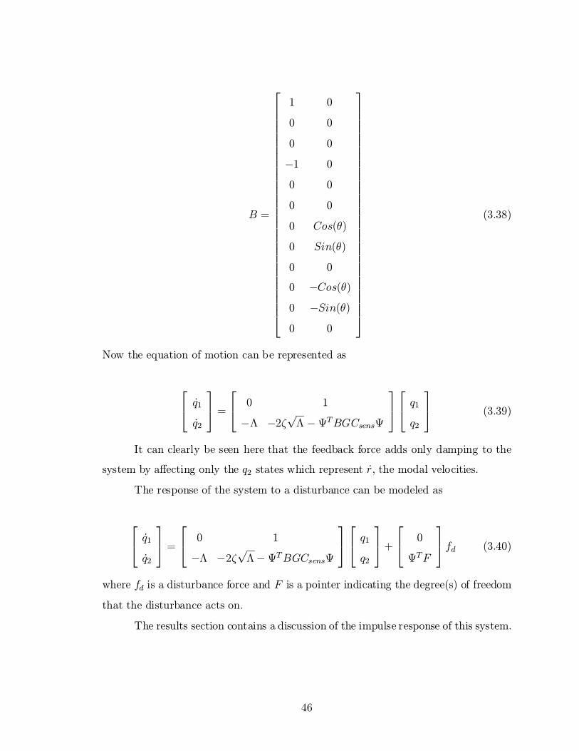
B =
26666666666666666666666666666664
1 0
0 0
0 0
¡1 0
0 0
0 0
0 Cos(µ)
0 Sin(µ)
0 0
0 ¡Cos(µ)0 ¡Sin(µ)0 0
37777777777777777777777777777775
(3.38)
Now the equation of motion can be represented as
24 _q1
_q2
35 =
24 0 1
¡¤ ¡2³p
¤ ¡ªTBGCsensª
3524 q1
q2
35 (3.39)
It can clearly be seen here that the feedback force adds only damping to the
system by a®ecting only the q2 states which represent _r, the modal velocities.
The response of the system to a disturbance can be modeled as
24 _q1
_q2
35 =
24 0 1
¡¤ ¡2³p
¤¡ªTBGCsensª
3524 q1
q2
35+
24 0
ªTF
35 fd (3.40)
where fd is a disturbance force and F is a pointer indicating the degree(s) of freedom
that the disturbance acts on.
The results section contains a discussion of the impulse response of this system.
46
3.4 Summary
The force applied to the torus by the piezo actuators has been modeled using Bernoulli-
Euler beam theory. Using this simpli¯cation, the piezo lm measures the di®erence
between the rotations at its ends. The piezo also produces two opposing moments at
its ends when a voltage is applied to it.
Pole placement techniques are initially examined to attenuate vibration in the
torus. Full state modal feedback is originally assumed to develop the equations.
Using full state feedback the control force is assumed to depend on all of the states of
the model. Next a modal observer is designed based on using the piezos as position
and velocity sensors. Using the modal observer, the control force is based on the
estimated states. The observer has dynamics which doubles the number of poles in
the total system. The problem of observation spillover can make an observer-based
controller go unstable. The use of optimal control is discussed as a preferred method
for choosing the control gains.
Finally a simpler controller is designed using velocity output feedback. Velocity
feedback is a simple method of controlling a structure but has the disadvantage that
it does not roll o® at high frequencies. Another disadvantage of velocity feedback is
that the freedom to shape the closed loop response is much more limited.
These controllers are not chosen because they are the best for this application.
They are chosen as a simple and e®ective demonstration of the control of an in°atable
structure.
47
Chapter 4
Results
4.1 Introduction
The aspect ratio and in°ation pressure of an in°ated torus has signi¯cant e®ect on its
dynamics. Case studies of di®erent aspect ratios, in°ation pressures, and the e®ect of
adding PVDF patches to the torus are examined in this section. Two control methods
are examined, observer based state feedback and direct output velocity feedback.
Optimal control is explored as a method for choosing the controller gains. The time
response to an impulse excitation for both observer based state feedback and velocity
feedback control methods are presented. The e®ect of observer spillover is examined
for two di®erent observer designs and the importance of considering observer spillover
is illustrated.
4.2 E®ect of Torus Aspect Ratio on Mode Shapes
The aspect ratio of the torus has a signi¯cant impact on not only the natural fre-
quencies of the torus, but also on the mode shapes. The aspect ratio of a torus is
de¯ned by the radius of the tube divided by the radius of the ring, see Figure 1.2. The
torus of interest here has a small aspect ratio so all of the lower modes are orthogonal
pairs of ring modes, alternating in and out of the plane of the torus. Looking at
the higher order modes of the torus, di®erent types of modes are found. There are
48

Table 4.1: Frequencies for Toroids of Di®erent Aspect Ratios
A. Ratio 0.04 A. Ratio 0.08 A. Ratio 0.16 A. Ratio 0.32Mode 1 3.40653 5.41651 8.6288 13.1871Mode 2 3.40653 5.41651 8.6288 13.1871Mode 3 5.00177 7.62025 11.24832 15.0978Mode 4 5.00177 7.62025 11.24832 15.0978Mode 5 7.6564 12.67014 20.02911 21.83219Mode 6 7.6564 12.67014 20.02911 25.85162Mode 7 8.76011 13.95878 20.92717 26.78526Mode 8 8.76011 13.95878 20.92717 26.78534Mode 9 13.00151 21.6558 28.04733 27.51872Mode 10 13.00151 21.65581 29.48152 27.51872Mode 11 13.75096 22.32614 32.4445 28.0326Mode 12 13.75096 22.32614 32.4445 28.03261Mode 13 19.4775 27.9986 32.57246 28.32397Mode 14 19.4775 31.91182 32.57248 28.32399
sloshing modes, where the tube expands and contracts from side to side, breathing
modes, where the torus expands and contracts uniformly, axisymmetric modes like
those studied by Liepins [16], and many other types of motions. The important fact
is this, as the torus aspect ratio increases, these types of modes start to show up in
the lower order modes. In general, the sequence of the modes, especially the higher
order modes, changes signi¯cantly as the aspect ratio increases. Table 4.1 compares
the natural frequencies of four toroids with di®erent aspect ratios, these toroids do
not have PVDF patches. The ring diameter is held constant for each of the models,
at 15.24m (600 in). Each of the models is meshed with 60 elements around the ring
diameter and 12 elements around the tube diameter. The ¯rst model, with an aspect
ratio of 0.04, has the dimensions of interest here. The Appendix contains plots of the
¯rst fourteen modes of the toroids with aspect ratios of 0.04 and 0.32.
The signi¯cant impact on mode shapes with changing aspect ratio is very
important. For a torus with the aspect ratio of a car tire inner tube, there may be only
a few ring modes present. This can have a signi¯cant impact on experimental work
when trying to measure the mode shapes of a torus. This e®ect is also important when
49
considering active control of the torus because mode shapes directly impact modal
controllability and the placement of actuators and sensors. If the motion of the torus,
within the frequency range of interest, is not solely ring modes, the actuators may
need to be placed di®erently to create an e®ective controller.
4.3 Dynamic E®ect of Passive PVDF
Williams studied the dynamic e®ect of passive PVDF patches on a tensioned mem-
brane [24]. A passive PVDF patch refers to the dynamic e®ect of the PVDF consid-
ering only its mass and sti®ness without electric excitation. He found that adding the
PVDF lowered the natural frequencies of the tensioned membrane slightly but had
no signi¯cant e®ect on the mode shapes. Essentially the PVDF patch added mass
without signi¯cantly e®ecting the sti®ness.
Adding PVDF patches to the torus has a similar e®ect, considering the torus
The frequencies are lowered slightly but the mode shapes essentially remain the same
through the ¯rst 14 modes, at least for thin °exible patches and toroids of the aspect
ratio considered here. Figure 4.1 shows the e®ect of passive PVDF patches on the
natural frequency of the torus. Two PVDF con¯gurations were analyzed. The PVDF
was added ¯rst to just the outer surface of the torus. The second con¯guration had
PVDF patches on both the outer and the top surfaces of the torus, as de¯ned in
Figure 2.1.
The e®ect of the bonding process has not been considered in this model. The
additional mass is likely insigni¯cant but, depending on the bonding process used, the
sti®ness may be signi¯cantly increased. Signi¯cant increases in sti®ness could have
additional e®ects on the response of the torus. Careful choice of bonding techniques
should minimize changes to the dynamics of the torus.
50
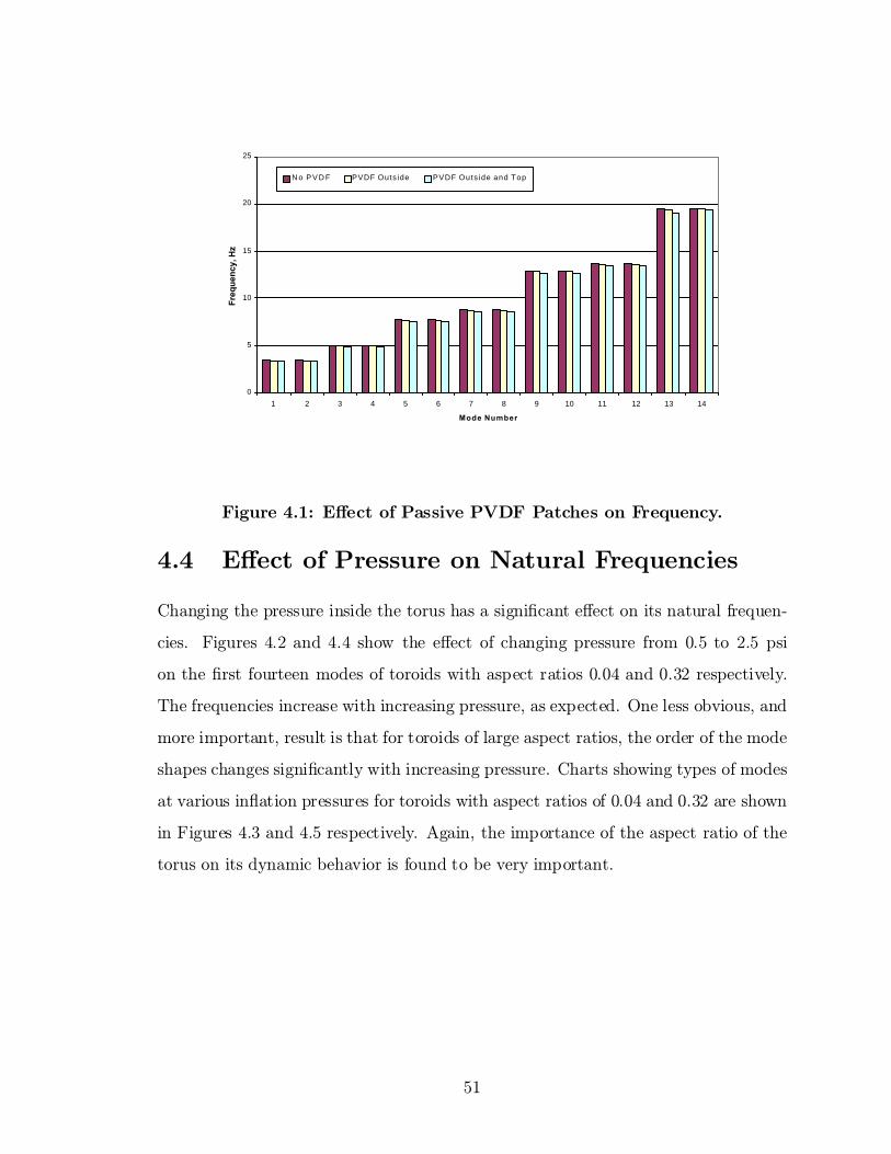
0
5
10
15
20
25
1 2 3 4 5 6 7 8 9 10 11 12 13 14
Mode Number
Fre
qu
en
cy, H
z
N o P V D F PVDF Outs ide PVDF Outs ide and Top
Figure 4.1: E®ect of Passive PVDF Patches on Frequency.
4.4 E®ect of Pressure on Natural Frequencies
Changing the pressure inside the torus has a signi¯cant e®ect on its natural frequen-
cies. Figures 4.2 and 4.4 show the e®ect of changing pressure from 0.5 to 2.5 psi
on the ¯rst fourteen modes of toroids with aspect ratios 0.04 and 0.32 respectively.
The frequencies increase with increasing pressure, as expected. One less obvious, and
more important, result is that for toroids of large aspect ratios, the order of the mode
shapes changes signi¯cantly with increasing pressure. Charts showing types of modes
at various in°ation pressures for toroids with aspect ratios of 0.04 and 0.32 are shown
in Figures 4.3 and 4.5 respectively. Again, the importance of the aspect ratio of the
torus on its dynamic behavior is found to be very important.
51

0
5
1 0
1 5
2 0
2 5
3 0
Mode 1
Mode 2
Mode 3
Mode 4
Mode 5
Mode 6
Mode 7
Mode 8
Mode 9
Mode 1
0
Mode 1
1
Mode 1
2
Mode 1
3
Mode 1
4
Fre
qu
en
cy
, H
z
0.5 Ps i
1 .0 Ps i
1 .5 Ps i
2 .0 Ps i
2 .5 Ps i
Figure 4.2: E®ect of Pressure on Small Aspect Ratio (0.04) Torus NaturalFrequencies
Figure 4.3: E®ect of Pressure on Small Aspect Ratio (0.04) Torus ModeShapes
52
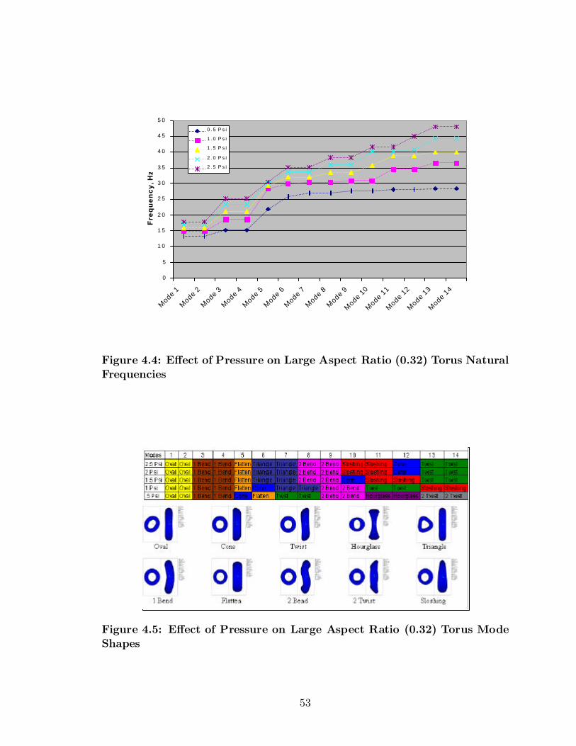
0
5
1 0
1 5
2 0
2 5
3 0
3 5
4 0
4 5
5 0
Mode 1
Mode 2
Mode 3
Mode 4
Mode 5
Mode 6
Mode 7
Mode 8
Mode 9
Mode 1
0
Mode 1
1
Mode 1
2
Mode 1
3
Mode 1
4
Fre
qu
en
cy
, H
z
0 . 5 P s i
1 . 0 P s i
1 . 5 P s i
2 . 0 P s i
2 . 5 P s i
Figure 4.4: E®ect of Pressure on Large Aspect Ratio (0.32) Torus NaturalFrequencies
Figure 4.5: E®ect of Pressure on Large Aspect Ratio (0.32) Torus ModeShapes
53
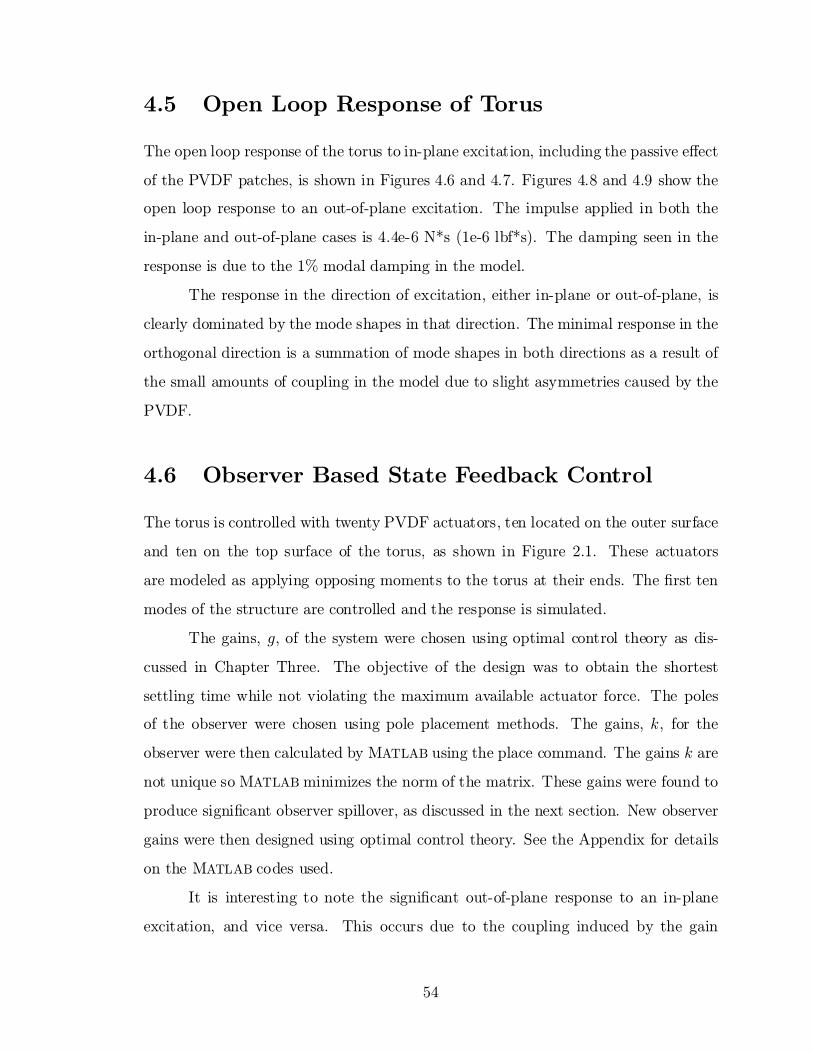
4.5 Open Loop Response of Torus
The open loop response of the torus to in-plane excitation, including the passive e®ect
of the PVDF patches, is shown in Figures 4.6 and 4.7. Figures 4.8 and 4.9 show the
open loop response to an out-of-plane excitation. The impulse applied in both the
in-plane and out-of-plane cases is 4.4e-6 N*s (1e-6 lbf*s). The damping seen in the
response is due to the 1% modal damping in the model.
The response in the direction of excitation, either in-plane or out-of-plane, is
clearly dominated by the mode shapes in that direction. The minimal response in the
orthogonal direction is a summation of mode shapes in both directions as a result of
the small amounts of coupling in the model due to slight asymmetries caused by the
PVDF.
4.6 Observer Based State Feedback Control
The torus is controlled with twenty PVDF actuators, ten located on the outer surface
and ten on the top surface of the torus, as shown in Figure 2.1. These actuators
are modeled as applying opposing moments to the torus at their ends. The ¯rst ten
modes of the structure are controlled and the response is simulated.
The gains, g, of the system were chosen using optimal control theory as dis-
cussed in Chapter Three. The objective of the design was to obtain the shortest
settling time while not violating the maximum available actuator force. The poles
of the observer were chosen using pole placement methods. The gains, k, for the
observer were then calculated by MATLAB using the place command. The gains k are
not unique so MATLAB minimizes the norm of the matrix. These gains were found to
produce signi¯cant observer spillover, as discussed in the next section. New observer
gains were then designed using optimal control theory. See the Appendix for details
on the MATLAB codes used.
It is interesting to note the signi¯cant out-of-plane response to an in-plane
excitation, and vice versa. This occurs due to the coupling induced by the gain
54

0 5 1 0 1 5- 0 . 0 5
- 0 . 0 4
- 0 . 0 3
- 0 . 0 2
- 0 . 0 1
0
0 . 0 1
0 . 0 2
0 . 0 3
0 . 0 4
T i m e , s
Res
pons
e, m
icro
ns
S e t t l e T i m e : I n P l a n e 1 2 . 1 8 s , O u t o f P l a n e 9 . 3 0 s
I n P l a n e M o t i o n O u t o f P l a n e M o t i o n
Figure 4.6: Open Loop Impulse Response to In-Plane Excitation.
Figure 4.7: Open Loop Frequency Response to In-Plane Excitation.Y(1)=In-Plane-Response, Y(2)=Out-of-Plane Response
55
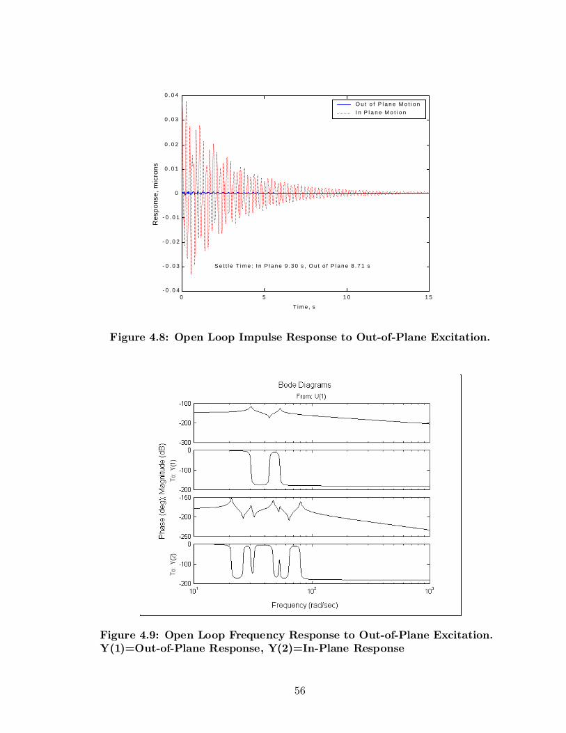
0 5 1 0 1 5- 0 . 0 4
- 0 . 0 3
- 0 . 0 2
- 0 . 0 1
0
0 . 0 1
0 . 0 2
0 . 0 3
0 . 0 4
T i m e , s
Res
pons
e, m
icro
ns
S e t t l e T i m e : I n P l a n e 9 . 3 0 s , O u t o f P l a n e 8 . 7 1 s
O u t o f P l a n e M o t i o nI n P l a n e M o t i o n
Figure 4.8: Open Loop Impulse Response to Out-of-Plane Excitation.
Figure 4.9: Open Loop Frequency Response to Out-of-Plane Excitation.Y(1)=Out-of-Plane Response, Y(2)=In-Plane Response
56
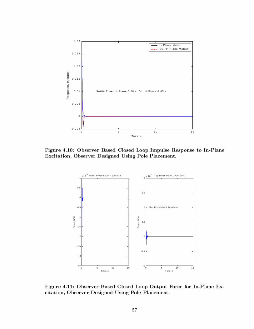
0 5 1 0 1 5- 0 . 0 0 5
0
0 . 0 0 5
0 . 0 1
0 . 0 1 5
0 . 0 2
0 . 0 2 5
0 . 0 3
S e t t l e T i m e : I n P l a n e 0 . 2 8 s , O u t o f P l a n e 0 . 4 5 s
T i m e , s
Res
pons
e, m
icro
ns
I n P l a n e M o t i o n O u t o f P l a n e M o t i o n
Figure 4.10: Observer Based Closed Loop Impulse Response to In-PlaneExcitation, Observer Designed Using Pole Placement.
0 5 1 0 1 5-3.5
-3
-2.5
-2
-1.5
-1
-0.5
0
0.5
1x 10
-4 Outer Piezo max=3.10e-004
Time, s
Fo
rce
, N
*m
0 5 1 0 1 5-1
-0.5
0
0.5
1
1.5
2x 10
-4 Top Piezo max=1.90e-004
Time, s
Max Possible=3.3e-4 N*m
Fo
rce
, N
*m
Figure 4.11: Observer Based Closed Loop Output Force for In-Plane Ex-citation, Observer Designed Using Pole Placement.
57

0 5 1 0 1 5- 0 . 0 1
- 0 . 0 0 5
0
0 . 0 0 5
0 . 0 1
0 . 0 1 5
0 . 0 2
0 . 0 2 5
S e t t l e T i m e : I n P l a n e 0 . 3 8 s , O u t o f P l a n e 0 . 4 6 s
T i m e , s
Res
pons
e, m
icro
ns
I n P l a n e M o t i o n O u t o f P l a n e M o t i o n
Figure 4.12: Observer Based Closed Loop Impulse Response to Out-of-Plane Excitation, Observer Designed Using Pole Placement.
0 5 10 15-10
-5
0
5x 10
- 5 Outer Piezo max=9.47e-005
Time, s
Forc
e, N
*m
0 5 10 15-2.5
-2
-1.5
-1
-0.5
0
0.5
1
1.5x 10
- 4 Top Piezo max=2.33e-004
Time, s
Max Possible=3.3e-4 N*m
Forc
e, N
*m
Figure 4.13: Observer Based Closed Loop Output Force for Out-of-PlaneExcitation, Observer Designed Using Pole Placement.
58

0 5 1 0 1 5- 0 . 0 1
- 0 . 0 0 5
0
0 . 0 0 5
0 . 0 1
0 . 0 1 5
0 . 0 2
0 . 0 2 5
S e t t l e T i m e : I n P l a n e 0 . 3 6 s , O u t o f P l a n e 0 . 4 6 s
T i m e , s
Res
pons
e, m
icro
ns
I n P l a n e M o t i o n O u t o f P l a n e M o t i o n
Figure 4.14: Observer Based Closed Loop Impulse Response to In-PlaneExcitation, Observer Designed Using Optimal Control.
0 5 1 0 1 5-1
-0.5
0
0.5
1
1.5
2
2.5
3
3.5x 10
-4Outer Piezo max=3.24e-004
Time, s
For
ce, N
*m
0 5 1 0 1 5-16
-14
-12
-10
-8
-6
-4
-2
0
2
4x 10
-5 Top P iezo max=1.45e-004
Time, s
Max Possib le=3.3e-4 N*m
For
ce, N
*m
Figure 4.15: Observer Based Closed Loop Output Force for In-Plane Ex-citation, Observer Designed Using Optimal Control.
59
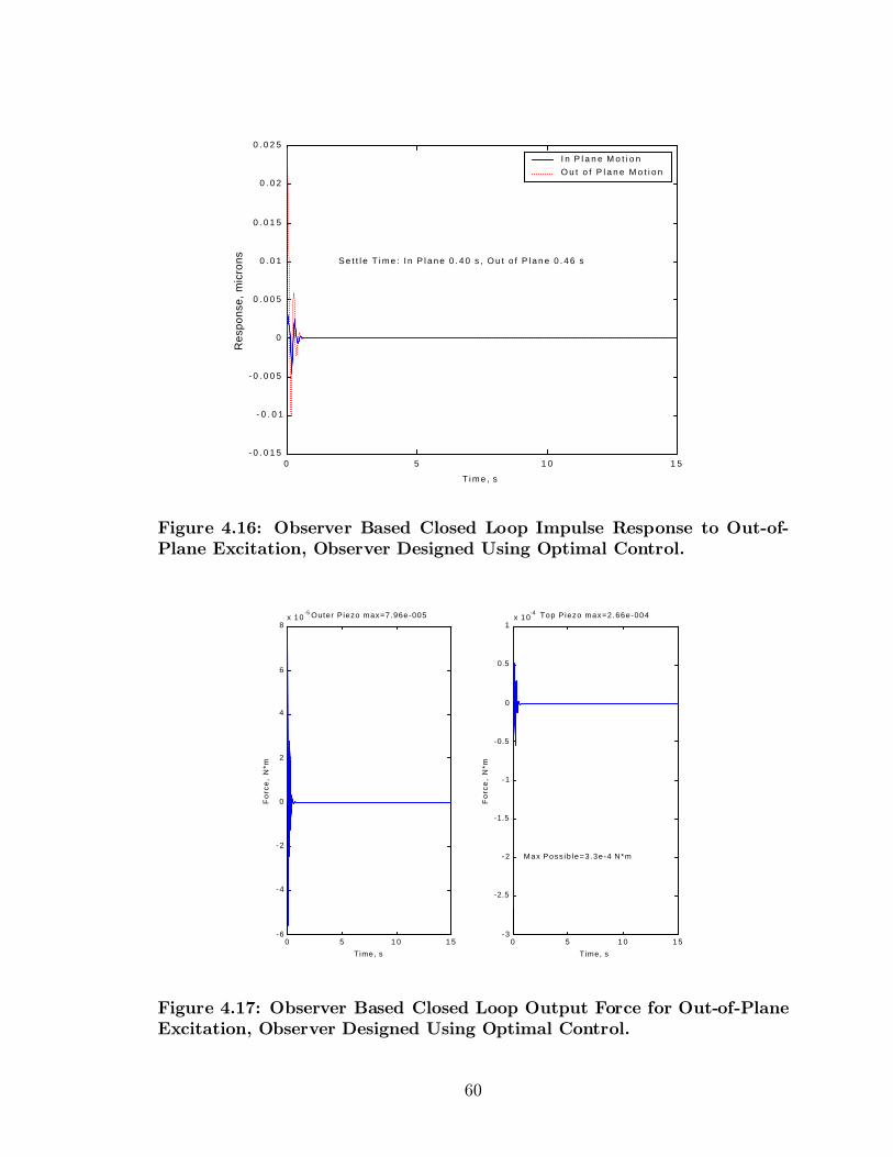
0 5 1 0 1 5- 0 . 0 1 5
- 0 . 0 1
- 0 . 0 0 5
0
0 . 0 0 5
0 . 0 1
0 . 0 1 5
0 . 0 2
0 . 0 2 5
S e t t l e T i m e : I n P l a n e 0 . 4 0 s , O u t o f P l a n e 0 . 4 6 s
T i m e , s
Res
pons
e, m
icro
ns
I n P l a n e M o t i o n O u t o f P l a n e M o t i o n
Figure 4.16: Observer Based Closed Loop Impulse Response to Out-of-Plane Excitation, Observer Designed Using Optimal Control.
0 5 1 0 1 5-6
-4
-2
0
2
4
6
8x 10
-5 Outer Piezo max=7.96e-005
Time, s
Fo
rce
, N
*m
0 5 1 0 1 5-3
-2.5
-2
-1.5
-1
-0.5
0
0.5
1x 10
-4 Top Piezo max=2.66e-004
Time, s
Max Poss ib le=3.3e-4 N*m
Fo
rce
, N
*m
Figure 4.17: Observer Based Closed Loop Output Force for Out-of-PlaneExcitation, Observer Designed Using Optimal Control.
60
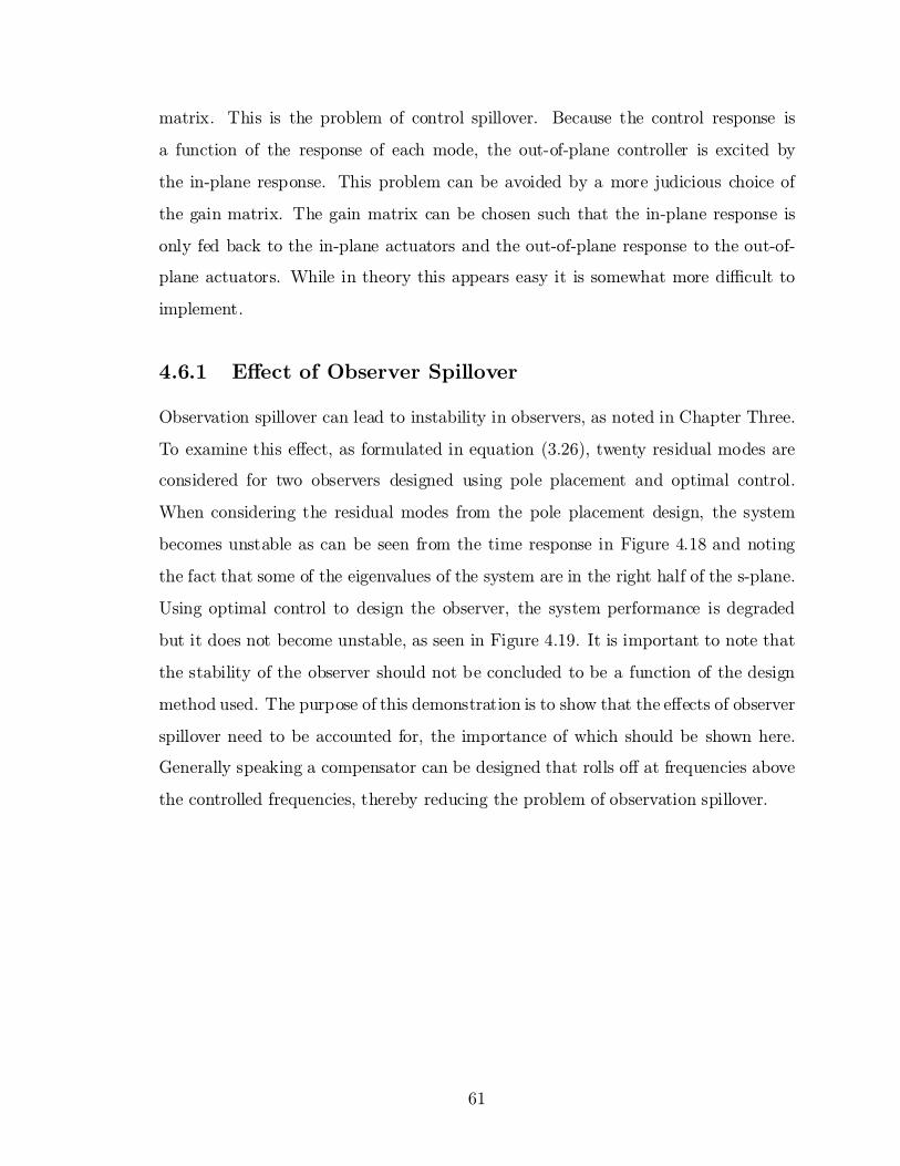
matrix. This is the problem of control spillover. Because the control response is
a function of the response of each mode, the out-of-plane controller is excited by
the in-plane response. This problem can be avoided by a more judicious choice of
the gain matrix. The gain matrix can be chosen such that the in-plane response is
only fed back to the in-plane actuators and the out-of-plane response to the out-of-
plane actuators. While in theory this appears easy it is somewhat more di±cult to
implement.
4.6.1 E®ect of Observer Spillover
Observation spillover can lead to instability in observers, as noted in Chapter Three.
To examine this e®ect, as formulated in equation (3.26), twenty residual modes are
considered for two observers designed using pole placement and optimal control.
When considering the residual modes from the pole placement design, the system
becomes unstable as can be seen from the time response in Figure 4.18 and noting
the fact that some of the eigenvalues of the system are in the right half of the s-plane.
Using optimal control to design the observer, the system performance is degraded
but it does not become unstable, as seen in Figure 4.19. It is important to note that
the stability of the observer should not be concluded to be a function of the design
method used. The purpose of this demonstration is to show that the e®ects of observer
spillover need to be accounted for, the importance of which should be shown here.
Generally speaking a compensator can be designed that rolls o® at frequencies above
the controlled frequencies, thereby reducing the problem of observation spillover.
61
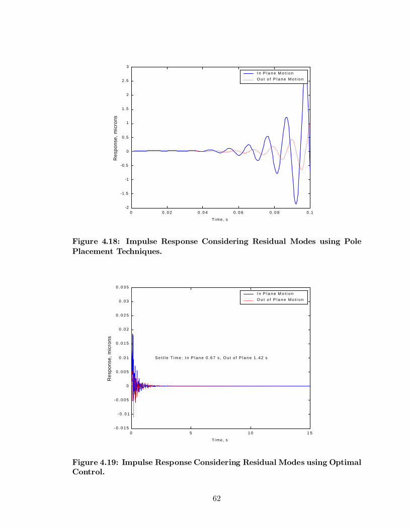
0 0 . 0 2 0 . 0 4 0 . 0 6 0 . 0 8 0.1-2
-1.5
-1
-0.5
0
0.5
1
1.5
2
2.5
3
T i m e , s
Res
pons
e, m
icro
ns
I n P l a n e M o t i o n O u t o f P l a n e M o t i o n
Figure 4.18: Impulse Response Considering Residual Modes using PolePlacement Techniques.
0 5 1 0 1 5- 0 . 0 1 5
- 0 . 0 1
- 0 . 0 0 5
0
0 . 0 0 5
0 . 0 1
0 . 0 1 5
0 . 0 2
0 . 0 2 5
0 . 0 3
0 . 0 3 5
T i m e , s
Res
pons
e, m
icro
ns
S e t t l e T i m e : I n P l a n e 0 . 6 7 s , O u t o f P l a n e 1 . 4 2 s
I n P l a n e M o t i o n O u t o f P l a n e M o t i o n
Figure 4.19: Impulse Response Considering Residual Modes using OptimalControl.
62

4.7 Results of Velocity Feedback Control
The torus is controlled with twenty PVDF actuators, ten located on the outer surface
and ten on the top surface of the torus, as shown in Figure 2.1. These actuators
are modeled as applying opposing moments to the torus at their ends. The ¯rst ten
modes of the structure are controlled and their response is simulated. The e®ect of
the velocity feedback controller on the higher order modes is not considered here.
Velocity feedback does not roll o® at high frequencies, so the in°uence of the higher
order modes can be signi¯cant.
The velocity feedback controller was able to reduce the impulse response set-
tling time to about 1 second, based on a 5% of max value settling criteria. The
impulse applied was 4.4e-6 N*s (1e-6 lbf*s). The in-plane and out-of-plane impulse
responses are shown in Figures 4.20 and 4.22. The maximum actuator force, for both
the top and outer actuators is shown for each case in Figures 4.21 and 4.23.
63
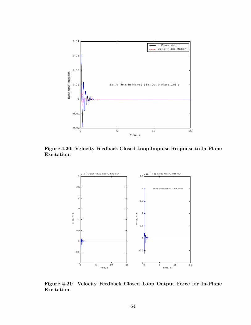
0 5 1 0 1 5- 0 . 0 2
- 0 . 0 1
0
0 . 0 1
0 . 0 2
0 . 0 3
0 . 0 4
S e t t l e T i m e : I n P l a n e 1 . 1 3 s , O u t o f P l a n e 1 . 0 8 s
T i m e , s
Res
pons
e, m
icro
ns
I n P l a n e M o t i o n O u t o f P l a n e M o t i o n
Figure 4.20: Velocity Feedback Closed Loop Impulse Response to In-PlaneExcitation.
0 5 1 0 1 5-1
-0.5
0
0.5
1
1.5
2
2.5
3x 10
- 4 Outer Piezo max=2.63e-004
Time, s
Fo
rce
, N
*m
0 5 1 0 1 5-1
-0.5
0
0.5
1
1.5
2
2.5x 10
- 4 Top Piezo max=2.03e-004
Time, s
Max Possible=3.3e-4 N*m
Fo
rce
, N
*m
Figure 4.21: Velocity Feedback Closed Loop Output Force for In-PlaneExcitation.
64
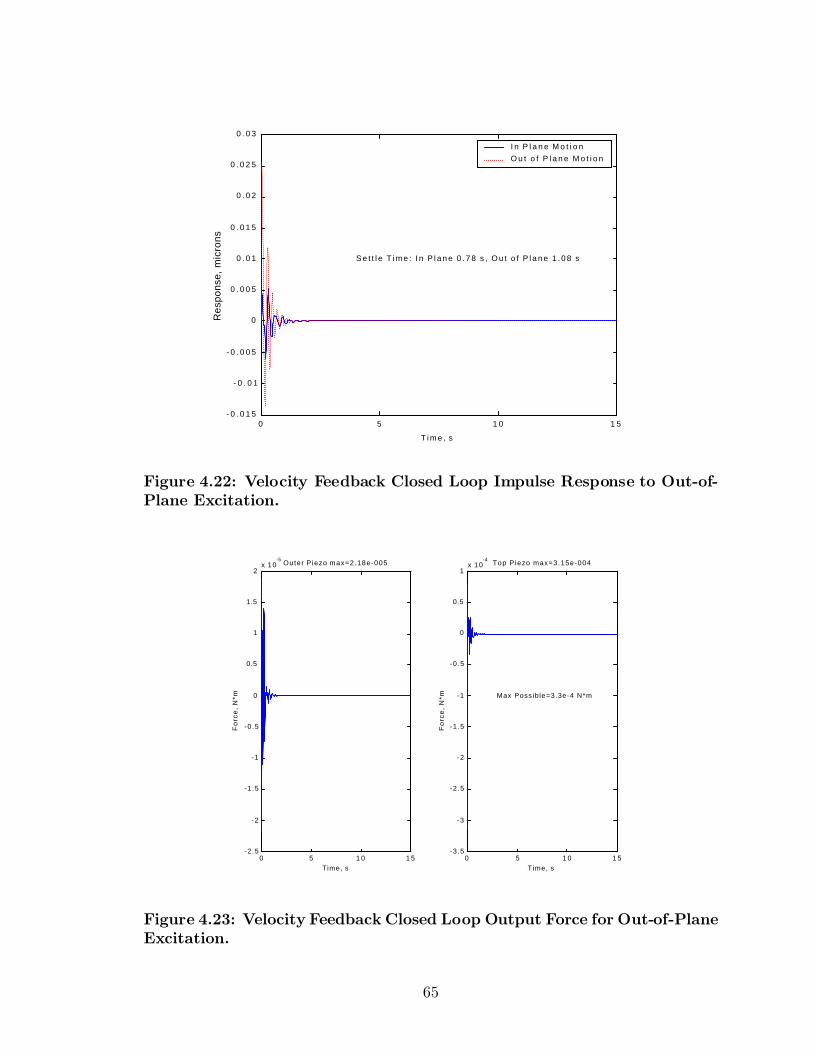
0 5 1 0 1 5- 0 . 0 1 5
- 0 . 0 1
- 0 . 0 0 5
0
0 . 0 0 5
0 . 0 1
0 . 0 1 5
0 . 0 2
0 . 0 2 5
0 . 0 3
S e t t l e T i m e : I n P l a n e 0 . 7 8 s , O u t o f P l a n e 1 . 0 8 s
T i m e , s
Res
pons
e, m
icro
ns
I n P l a n e M o t i o n O u t o f P l a n e M o t i o n
Figure 4.22: Velocity Feedback Closed Loop Impulse Response to Out-of-Plane Excitation.
0 5 1 0 1 5-2.5
-2
-1.5
-1
-0.5
0
0.5
1
1.5
2x 10
-5 Outer Piezo max=2.18e-005
Time, s
Fo
rce
, N
*m
0 5 1 0 1 5-3.5
-3
-2.5
-2
-1.5
-1
-0.5
0
0.5
1x 10
-4 Top Piezo max=3.15e-004
Time, s
Max Possible=3.3e-4 N*m
Fo
rce
, N
*m
Figure 4.23: Velocity Feedback Closed Loop Output Force for Out-of-PlaneExcitation.
65
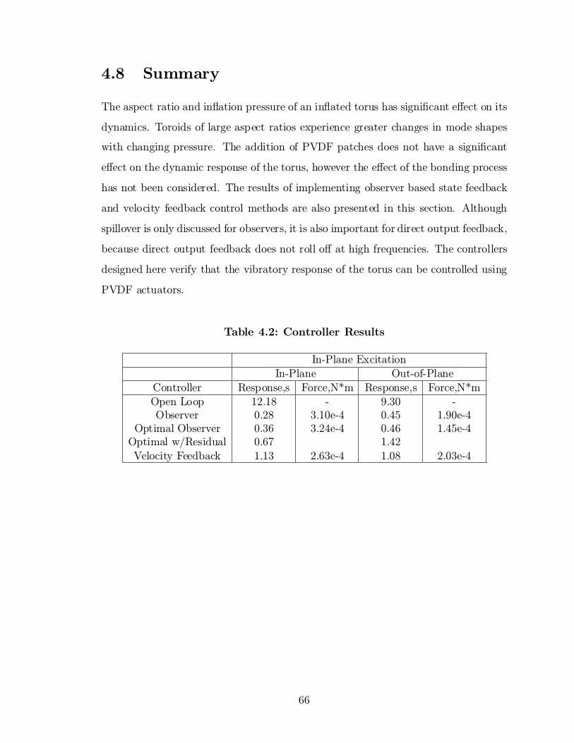
4.8 Summary
The aspect ratio and in°ation pressure of an in°ated torus has signi¯cant e®ect on its
dynamics. Toroids of large aspect ratios experience greater changes in mode shapes
with changing pressure. The addition of PVDF patches does not have a signi¯cant
e®ect on the dynamic response of the torus, however the e®ect of the bonding process
has not been considered. The results of implementing observer based state feedback
and velocity feedback control methods are also presented in this section. Although
spillover is only discussed for observers, it is also important for direct output feedback,
because direct output feedback does not roll o® at high frequencies. The controllers
designed here verify that the vibratory response of the torus can be controlled using
PVDF actuators.
Table 4.2: Controller Results
In-Plane ExcitationIn-Plane Out-of-Plane
Controller Response,s Force,N*m Response,s Force,N*mOpen Loop 12.18 - 9.30 -Observer 0.28 3.10e-4 0.45 1.90e-4
Optimal Observer 0.36 3.24e-4 0.46 1.45e-4Optimal w/Residual 0.67 1.42Velocity Feedback 1.13 2.63e-4 1.08 2.03e-4
66

Chapter 5
Conclusions
5.1 Introduction
This thesis has investigated the feasibility of using PVDF to attenuate vibration in an
in°ated torus. To this end, the dynamics of the free-free torus have been investigated.
The passive e®ect of adding PVDF to the structure has been examined. Finally a
state space model has been created to implement standard control techniques to
demonstrate the controllability of the structure using PVDF actuation.
5.2 Key Results
The in°ation pressure and aspect ratio of a torus are found to have signi¯cant impact
on its dynamic response. Increasing the in°ation pressure generally increases the
natural frequencies of the torus. This result should be expected since increasing
in°ation pressure essentially sti®ens the torus. The vibratory response of toroids
with small aspect ratios, skinny tubes, is dominated by ring modes. When looking
at toroids with larger aspect ratios, toroids with fat tubes, the vibratory response
contains many di®erent types of modes. For this reason it may be more di±cult
to attenuate vibration in toroids with large aspect ratios. Also, increasing pressure
in toroids with large aspect ratios tends to a®ect the sequence of the modes. Any
structural-acoustic interaction that could occur is not considered.
67
Piezoelectric PVDF patches have a very limited e®ect on the vibratory response
of toroids with small aspect ratios, considering only their passive e®ect. Generally the
natural frequencies are decreased slightly, as should be expected by adding mass to
the system, but there is little in°uence on the mode shapes. Only part of the sti®ness
of the PVDF patch is considered because the PVDF and Kapton are assumed to lie
in the same plane instead of being layered.
Using a closed loop feedback system the vibratory response of an in°ated torus
can be attenuated signi¯cantly compared to its open loop response. The PVDF
is modeled very simply. This simple model can be questioned in two ways. Is it
appropriate to model the force transferred from the PVDF to the Kapton as two
opposing moments? Is the calculation of the maximum possible amount of force
generated by the PVDF correct? Vibratory control of an in°ated torus is shown
to be possible. The e®ect of spillover is signi¯cant when designing any vibration
suppression system and must be considered in order to produce a viable design.
5.3 Future Work
The torus model here was validated by analysis performed by Liepins in 1965. Liepins
analyzed and validated his models of in°ated toroids, but with signi¯cantly greater
sti®ness. Test validation for very thin in°ated shells is yet to be performed in detail.
The interaction between the PVDF and the host structure, the in°ated torus,
was treated as a beam. This is a great simpli¯cation of the structure. Much more
detailed analysis of the interaction between the actuator and the torus needs to be
performed to truly determine the potential e®ectiveness of vibration control of the
structure.
The dynamics of the torus are treated as being linear with small deformations.
These assumptions need to be investigated in detail to determine their validity. The
materials used in in°ated space structures often have signi¯cant nonlinear properties.
There is also an important question as to whether or not vibration of thin in°ated
structures can really be treated as small deformation problems. This author believes
68

that they can because the motion seen here is essentially motion of the entire tube,
not local deformation of the tube wall, however at present this question has not been
satisfactorily answered.
The control system designed here was not intended to produce an optimal
response. The purpose of this control design was to demonstrate control of the torus.
Practical implementation of control of this system demands a much more rigorous
control design considering robustness and, as shown here, spillover.
This work has considered only structures that rely mainly on in°ation pressure
for their structural sti®ness. Rigidization techniques are likely to be more popular
for production systems because they do not rely on an internal pressure to maintain
their sti®ness. The ability of piezoelectric devices to control rigidizable structures
needs to be examined.
69

Bibliography
[1] Agnes, Gregory S. and Rogers, James W., Piezoelectric Excitation of In°atable
Space Structures for Modal Testing. SPIE Smart Materials and Structures Con-
ference, March 2000.
[2] Cassapakis, C. and Mitch, T., In°atable Structures Technology Development
Overview. Paper 95-3738, AIAA, 1995.
[3] Chaudhry, Z. and Rogers, C.A., The Pin-Force Model Revisited. Journal of In-
telligent Material Systems and Structures, Vol. 5, May 1994, pp 347-354.
[4] Derbes, B., Case Studies in In°atable Rigidizable Structural Concepts for Space
Power. Paper 99-1089, AIAA, 1999.
[5] Dosch, J.J., Inman Daniel J., and Garcia E., A Self-Sensing Actuator for Col-
located Control. Journal of Intelligent Material Systems and Structures, Vol. 3,
No. 1, Jan 1992, pp 166-185.
[6] Freeland, R. E., Signi cance of the In°atable Antenna Experiment Technology.
Paper 98-2104, AIAA, 1998.
[7] Freeland, R.E., Bilyeu, G.D., and Veal, G.R., Development of Flight Hardware for
a Large, In°atable-Deployable Antenna Experiment, International Astronautical
Federation, Paper 95-1501, 1995.
[8] Freeland, R.E. and Bilyeu, G.D., In-Step In°atable Antenna Experiment, Inter-
national Austronautical Federation, Paper 92-0301, 1992.
70

[9] Friedland, Bernard, Control System Design, An Introduction to State-Space
Methods, McGraw Hill, Boston Massachusetts, 1986.
[10] Gri±th, D. Todd and Main, John A., Modal Testing of an In°ated Thin Film
Polyimide Torus Structure Proceedings, XVIII International Modal Analysis
Conference, Februrary 2000.
[11] Inman, Daniel J., Vibration with Control, Measurement, and Stability Prentice
Hall, New Jersey, 1989.
[12] Inman, Daniel J., Engineering Vibration Prentice Hall, New Jersey, 1996.
[13] Jordan, Peter F., Vibration Study of a Pressurized Torus Shell Part I - Experi-
mental Study. NASA CR-884, Oct. 1967.
[14] Jordan, Peter F., Vibration and Buckling of Pressurized Torus Shells. Paper 66-
445, AIAA, 1966, also presented at the AIAA 4th Aerospace Sciences Meeting
Los Angeles, CA June 27-29, 1966.
[15] Lassiter, John O., Engberg, Robert, Slade, Kara N., Tinker, Michael L., Com-
parison of Dynamic Characteristics for an In°atable Solar Concentrator in At-
mospheric and Thermal Vaccum Conditions. Paper 2000-1641, AIAA, 2000, Pre-
sented at the 41st Structures, Structural Dynamics, and Materials Conference
and Exhibit, Atlanta, GA, 3-8 April 2000.
[16] Liepins, Atis A., Free Vibrations of Prestressed Toroidal Membrane. AIAA Jour-
nal, Vol3, No. 10, Oct. 1965, pp. 1924-1933.
[17] Liepins, Atis A., Flexural Vibrations of the Prestressed Toroida Shell. NASA
CR-296, Sept. 1965.
[18] Liepins, Atis A., Vibration Study of a Pressurized Torus Shell Part II - Devel-
opment and Applications of Analysis. NASA CR-885, Oct. 1967.
[19] Meirovitch, Leonard, Control of Structures Wiley-Interscience, New York, 1990.
71

[20] Nurre, G.S., Sharkey, J.P., Nelson, J.D., and Bradley, A.J., Preservicing Mission,
On-Orbit Modi¯cations to the Hubble Space Telescope Pointing Control System.
AIAA Journal of Guidance, Control, and Dynamics, Vol. 18, No. 2, Mar.-Apr.
1995, pp 222-229.
[21] Preliminary Mission Report: Spartan 207/In°atable Antenna Experiment Flown
on STS-77, Spartan Project, NASA-GSFC, Feb. 14, 1997
[22] Rao, S. and Sunar, M., Piezoelectricity and its use in disturbance sensing and
control of °exible structures: A survey. Applied Mechanics Reviews, Vol. 47, No.
4, April 1994.
[23] Tinker, Michael L., Passively Adaptive In°atable Structure for the Shooting Star
Experiment. Paper 98-1986, AIAA, 1998.
[24] Williams, R.B., Experimental and Analytical Methods to Ascertain the E®ects of
Piezopolymer Actuators on the Dynamics of In°atable Space-Based Structures.
Virginia Tech MS Thesis, 2000.
72

Appendix A
Mode Shapes
The mode shapes of toroids of two di®erent aspect ratios are shown. The ¯rst torus
has an aspect ratio of 0.04 and the second torus has an aspect ratio of 0.32. The ¯rst
fourteen modes of the small aspect ratio torus are exclusively ring modes. The ¯rst
four modes of the torus with the large aspect ratio are ring modes, but then di®erent
types of modes are manifest. Both toroids are in°ated to 0.5 psi.
73
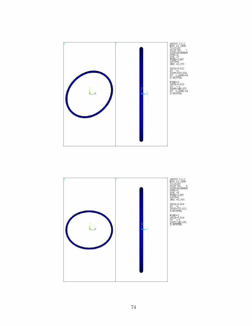
74
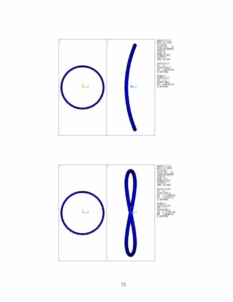
75
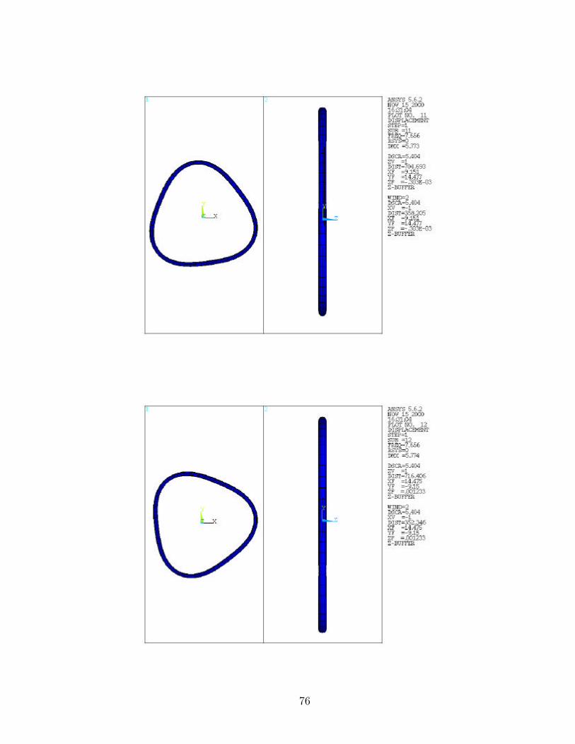
76
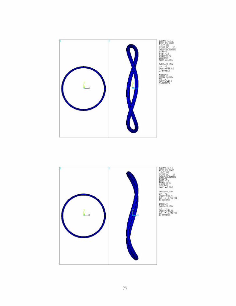
77

78
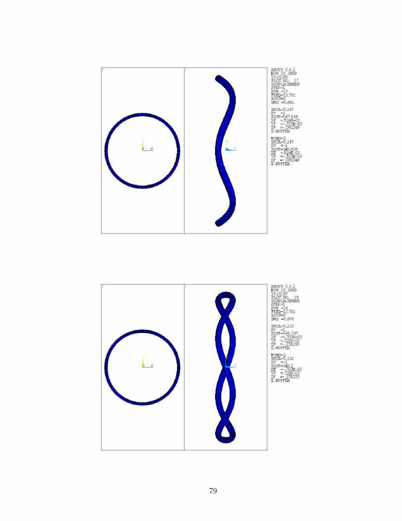
79
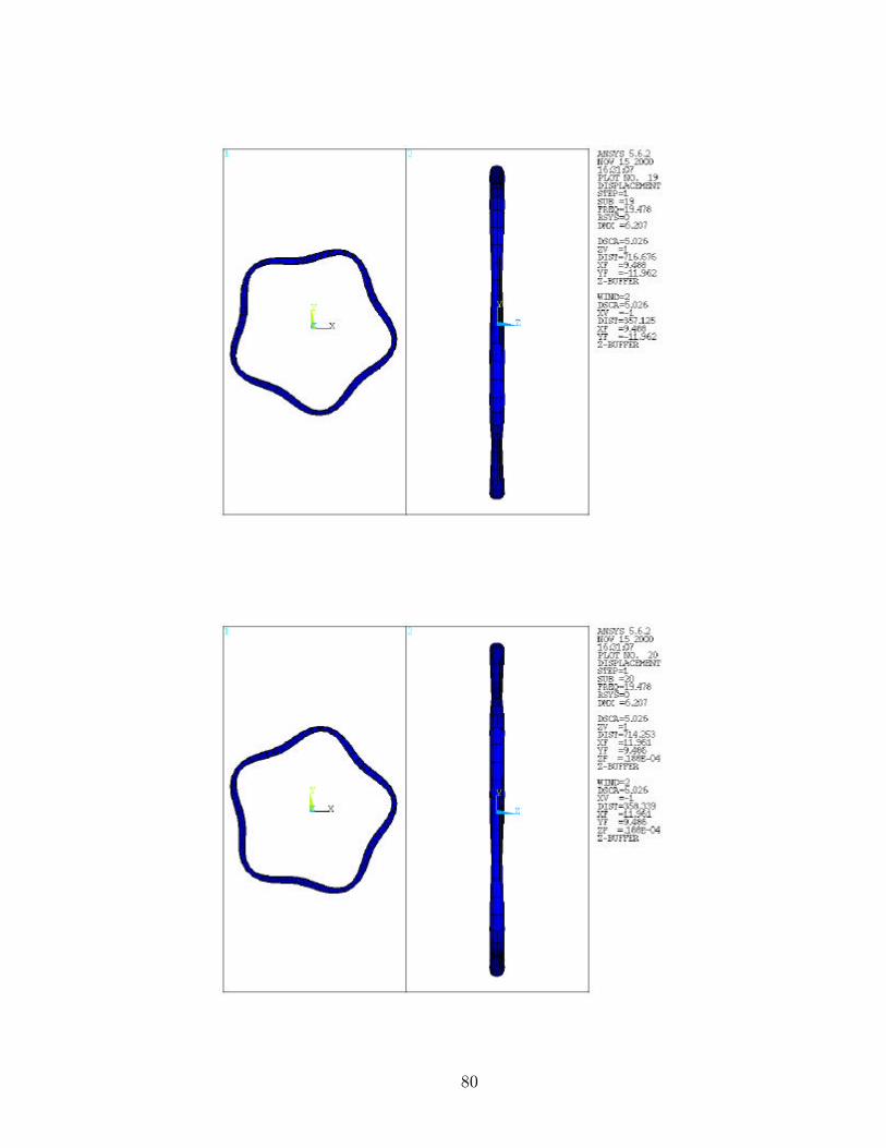
80

81
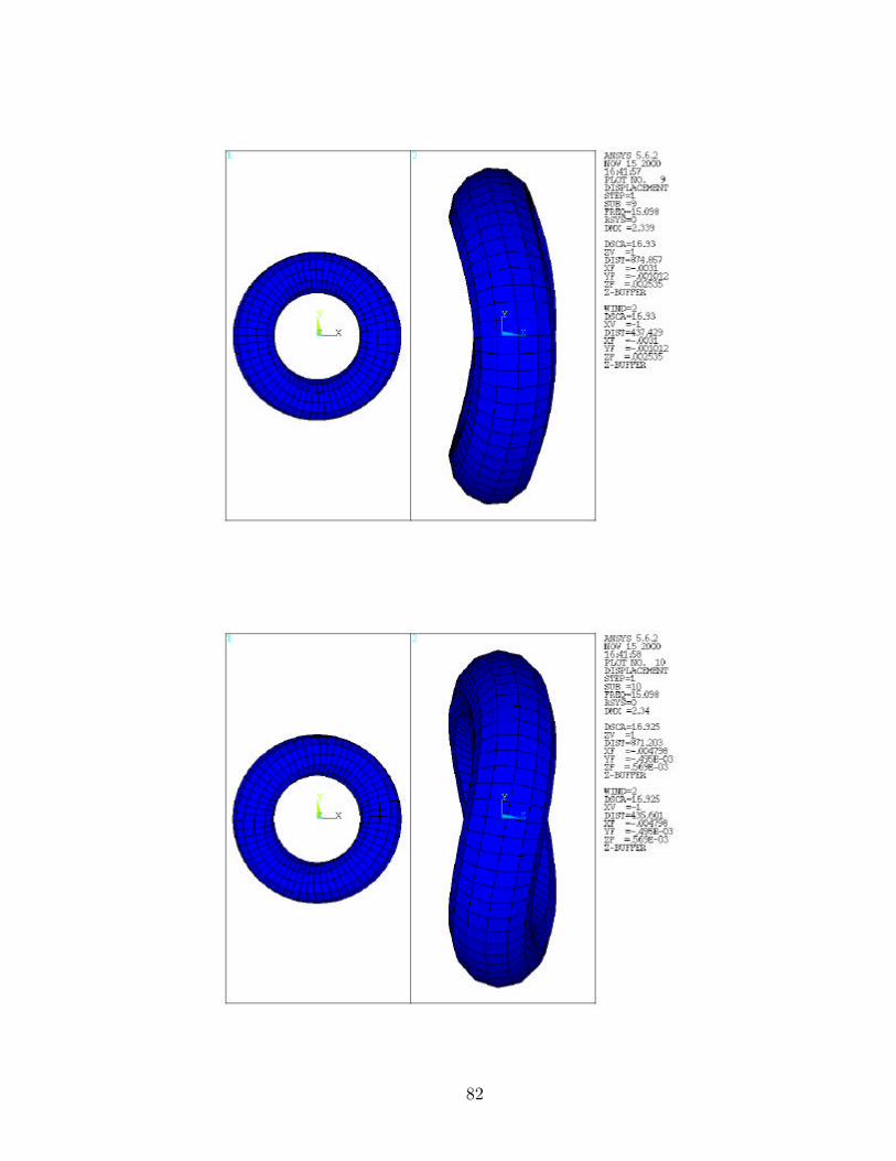
82
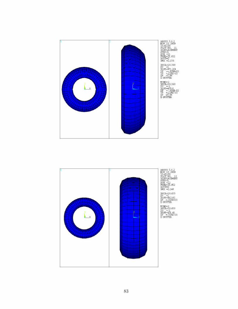
83
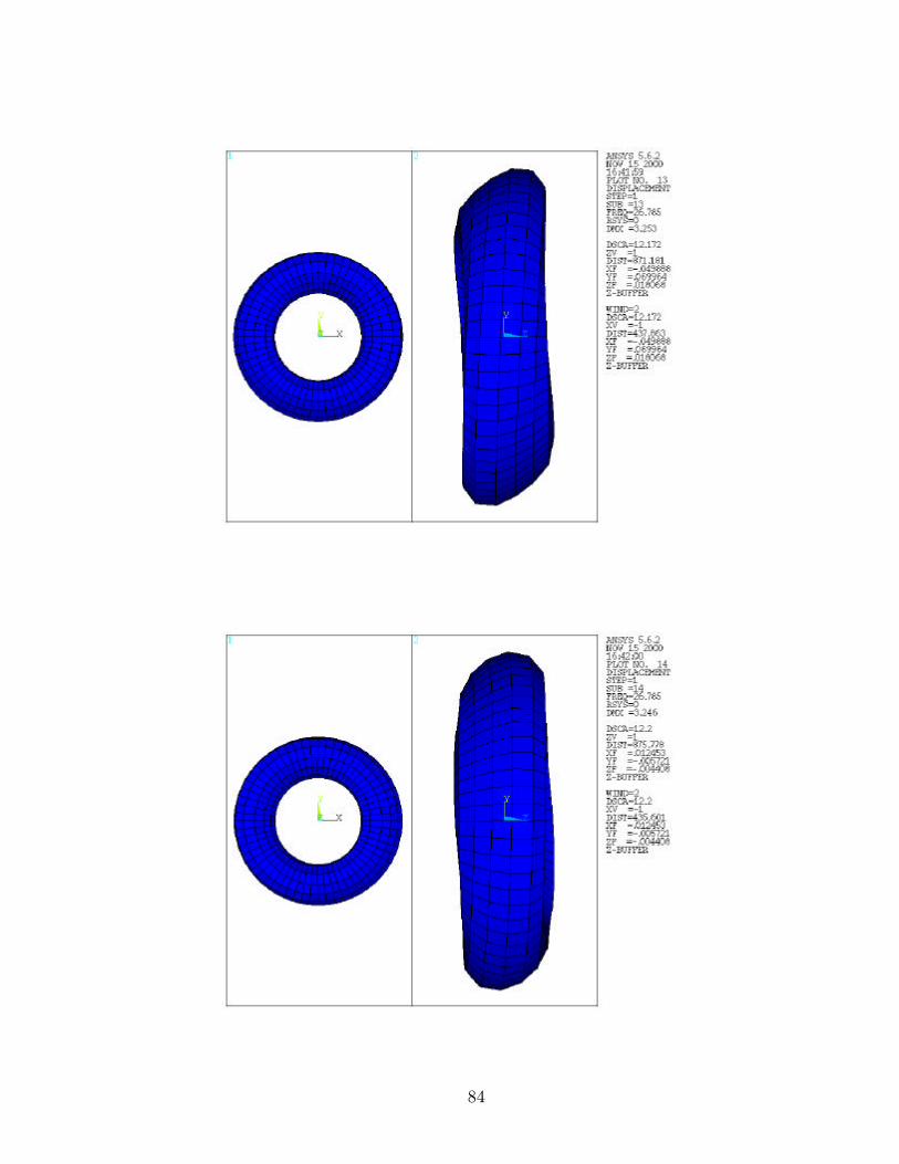
84

85
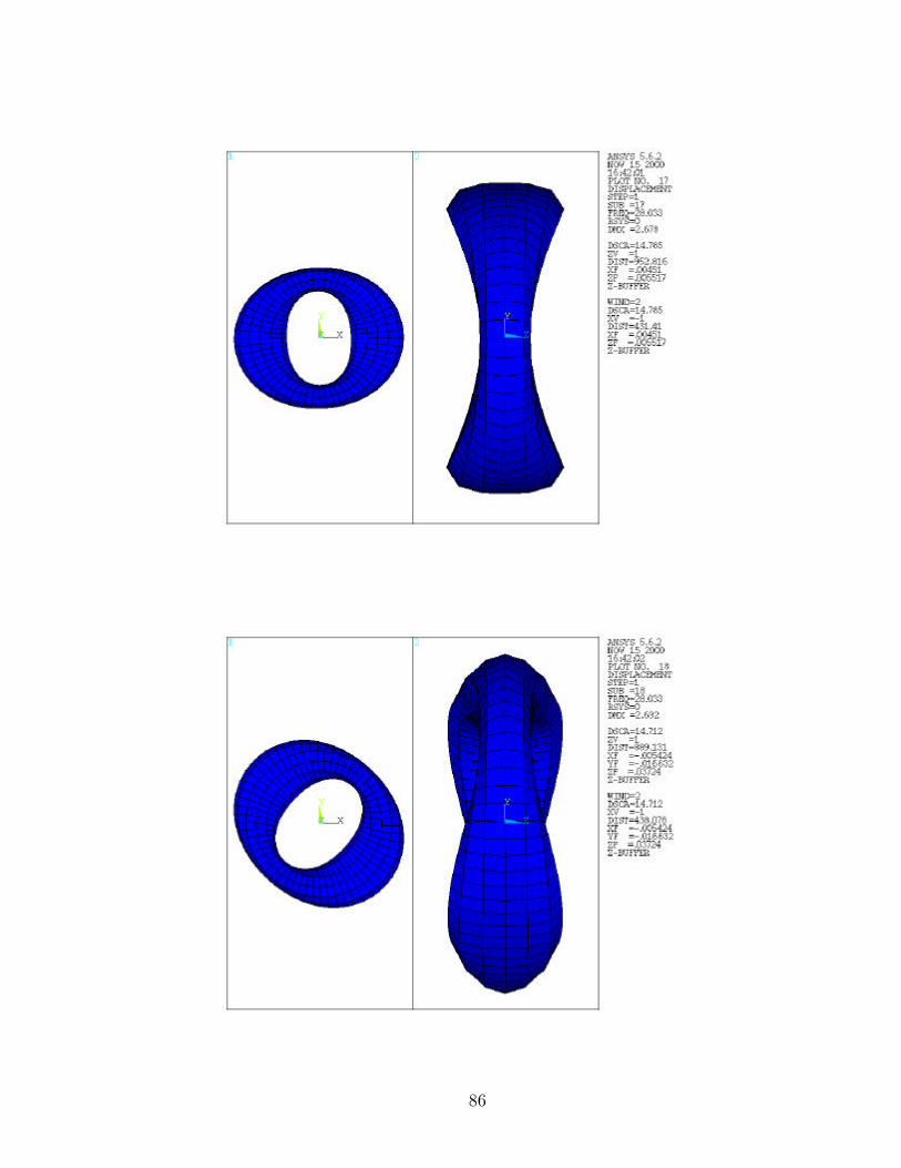
86
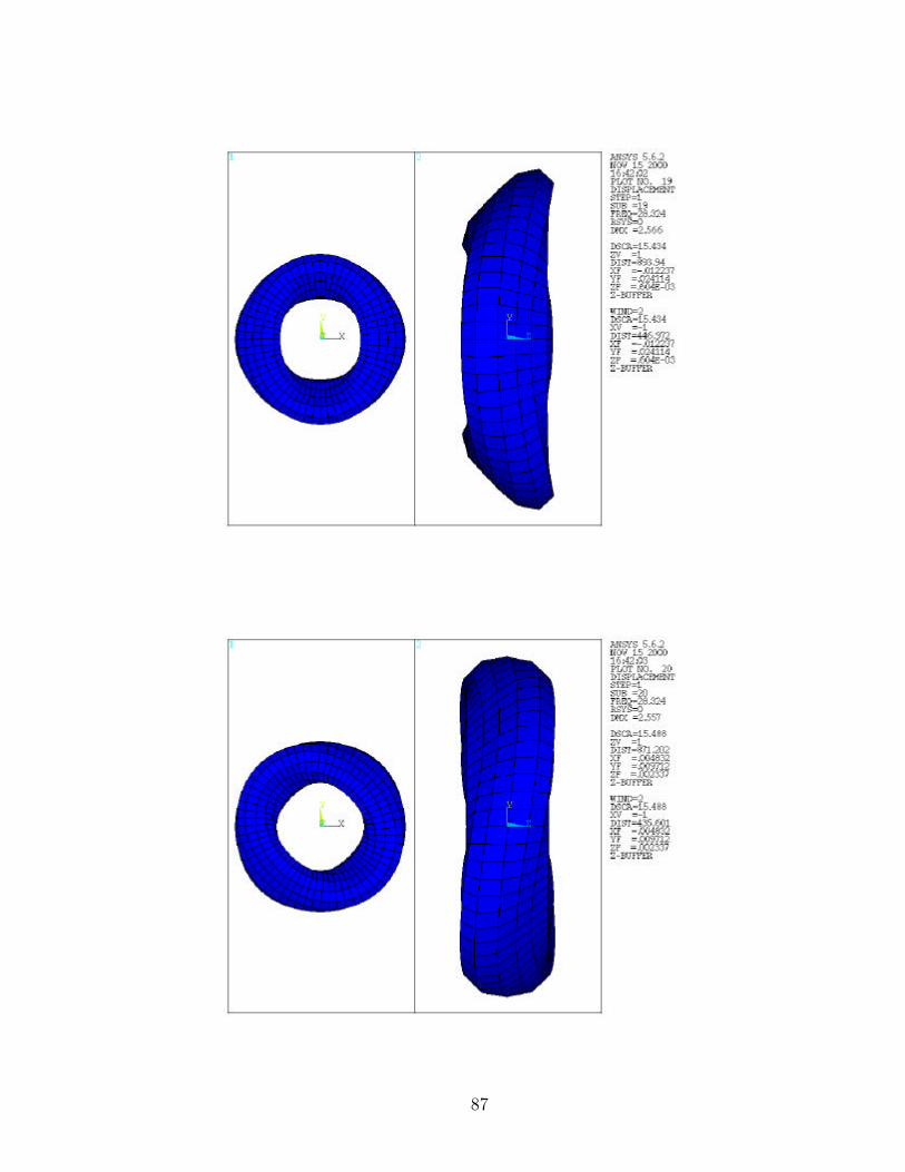
87

Appendix B
MATLAB Mesh Generation
% Generate node locations (x,y,z) and connectivity for a torus
% with major radius R0 and minor radius r0.
% The outputs of this file elem8.csv and node.csv can be manipulated
% in MS Excel to form appropraite input files to ANSYS.
% The output files are already in comma delimited format which is
% what ANSYS needs. Therefore just open them in Excel, edit the files
% and then save them again as comma delimited format.
% The node.csv file needs to be in the form:
% n, ,#,#,#
% This is accomplished by adding two columns to the worksheet in Excel
% and then filling the first with "n"s. Also, zero values are output
% as blanks so the three columns with numbers (only including the rows
% of interest) need to be highlighted and the replace all command needs
% to be used, replacing all blank values with "0"s.
% The elem8.csv file needs to be in the form:
% e,#,#,#,#,#,#,#,#
% This is accomplished by adding one column to the worksheet in Excel
% and then filling it with "e"s.
% Jackson A. Lewis 12/00
% Originally Written by Eric M. Austin. 9/22/99
clear all
close all
% Number of elements in the circumferencial direction (angle eta), i.e.,
% around the large, outer circle of the torus
88

num_c_elem = 30;
% Number of elements in the radial direction (angle eta), i.e.,
% around the smaller tube
num_r_elem = 8;
num_r_elem = num_r_elem*2;
num_c_elem = num_c_elem*2;
nelem = num_c_elem*num_r_elem;
% Dimensions
R0 = 300; % major radius
r0 = 12; % minor radius
%%%%%%%%%%%%%%%%%%%%%%%%%%%%%%%%%%%%%%%%%%%%%%%%%%%%%%%%%%%%%%%%%%%%%%%%%%
% Build the mesh as a flat domain and match up node numbers at the end.
% This is a single strip (0 -> 2 pi) around the outer diameter of the torus.
% The ends are matched up, so this is a complete hoop.
basic_strip = [(1:num_c_elem)' , ...
[(2:num_c_elem) 1]' , ...
((num_c_elem+1):(2*num_c_elem))' , ...
[((num_c_elem+2):(2*num_c_elem)) (num_c_elem+1)]'];
% dimension the connectivity matrix
con = zeros(num_r_elem*num_c_elem,4);
% Duplicate the "basic_strip" above for each strip around the smaller tube.
for ir = 1:num_r_elem
con(((ir-1)*num_c_elem+1):ir*num_c_elem,:) = (ir-1)*num_c_elem + basic_strip;
end
% Connect the last row to the first
con(((num_r_elem-1)*num_c_elem+1):num_r_elem*num_c_elem,3:4) = basic_strip(:,1:2);
con2=zeros(num_r_elem*num_c_elem/4,8);
for i=0:num_c_elem/2-1
for j=0:num_r_elem/2-1
con2((i+1)+(j*num_c_elem/2),:)=[con(2*j*num_c_elem+2*i+1,1), ...
con(2*j*num_c_elem+2*i+2,2), ...
con((2*j+1)*num_c_elem+2*i+2,4),con((2*j+1)*num_c_elem+2*i+1,3), ...
con(2*j*num_c_elem+2*i+2,1),con(2*j*num_c_elem+2*i+2,4), ...
con((2*j+1)*num_c_elem+2*i+1,4),con((2*j+1)*num_c_elem+2*i+1,1)] ;
end
end
89

% node locations
% XI and ETA are square meshes for now. See MATLAB manual for use of MESHGRID
[XI,ETA]=meshgrid(linspace(0,2*pi,num_r_elem+1),linspace(0,2*pi,num_c_elem+1));
local_xi = zeros(num_r_elem*num_c_elem,1);
local_eta = zeros(num_r_elem*num_c_elem,1);
% "Pour" them into a long vector that lines with the node numbers
local_xi(:) = XI(1:num_c_elem,1:num_r_elem);
local_eta(:) = ETA(1:num_c_elem,1:num_r_elem);
% Standard equation for x, y, and z coordinates of a torus
xyz_loc = [(R0 + r0*cos(local_xi)) .* cos(local_eta) , ...
(R0 + r0*cos(local_xi)) .* sin(local_eta) , r0*sin(local_xi)];
% Plot 4 Node Elements
figure
for i = 1:nelem
line(xyz_loc(con(i,[1 2 4 3 1]),1),xyz_loc(con(i,[1 2 4 3 1]),2), ...
xyz_loc(con(i,[1 2 4 3 1]),3))
end
title(['Four Node Torus with major radius ' num2str(R0) ' and minor radius ' ...
num2str(r0) ', ' int2str(nelem) ' nodes and elements.'])
view([0 30])
axis equal
axis off
%Plot 8 Node Elements
figure
for i = 1:nelem/4
line(xyz_loc(con2(i,[1 5 2 6 3 7 4 8 1]),1) ...
,xyz_loc(con2(i,[1 5 2 6 3 7 4 8 1]),2) ...
,xyz_loc(con2(i,[1 5 2 6 3 7 4 8 1]),3))
end
title(['Eight Node Torus with major radius ' num2str(R0) ' and minor radius ' ...
num2str(r0) ', ' int2str(nelem) ' nodes and ' num2str(nelem/4) ' elements.'])
view([0 30])
axis equal
90

axis off
%Format for Ansys
cona=[con(:,1),con(:,2),con(:,4),con(:,3)];
dlmwrite('elem4.csv',cona)
dlmwrite('elem8.csv',con2)
dlmwrite('node.csv',xyz_loc)
91

Appendix C
MATLAB Eigenvalue Solution
% Solve Eigenvalue Problem
% Written By Jackson A. Lewis 12/00
clear all
close all
% Set Variables
f=1e-6; %Magnitude of Forcing Function
dofs=6; %Degrees of Freedom Per Node
%ndof=6000*6; %Total Degrees of Freedom in Model
criteria=0; %Criteria for guyan reduced DOF
%.001 means remove DOFS smaller than .001*largest
%0 means remove only massless dofs
nmcalc=30; %Number of Eigenvalues to Calculate
nmodes=10; %Number of Modes to Retain in modal truncation
%Must be <= nmcalc
%%%%%%%%%%%%%%%%%%%%%%%%%%%%%%%%%%%%%%%%%%%%%%%%%%%%%%%%%%%%%%%%%%%%%%%%%%%%
%%%%%%%%%%%%%%%%%%%%%%%%%%%%%%%%%%%%%%%%%%%%%%%%%%%%%%%%%%%%%%%%%%%%%%%%%%%%
% Read in unformatted mass and stiffness matrices
[m1,m2,m3]=textread('mass.txt','%u %u %f');
m=[m1,m2,m3];
[k1,k2,k3]=textread('stiff.txt','%u %u %f');
k=[k1,k2,k3];
% Number of DOF in Model
ndofm=max([max(m(:,1)),max(m(:,2))]);
ndofk=max([max(k(:,1)),max(m(:,2))]);
ndofc=max(ndofm,ndofk);
ndofc=dofs*ceil(ndofc/dofs);
%check=ndof-ndofc
ndof=ndofc
92

'Create Mass Matrix'
mm=sparse(m1,m2,m3,ndof,ndof);
%mm is only upper diagonal, now form full mm
mm=mm+mm'-diag(diag(mm));
'Mass Matrix Formulation Complete'
'Create Stiffness Matrix'
km=sparse(k1,k2,k3,ndof,ndof);
%km is only upper diagonal, now form full km
km=km+km'-diag(diag(km));
'Stiffness Matrix Formulation Complete'
clear k m k1 k2 k3 m1 m2 m3
%Remove DOFS w/ zero mass AND stiffness
%This only happens if there are applied bc's
%ie not a free vibration problem
[rowm,colm]=find(mm);
[rowk,colk]=find(km);
row=union(rowm,rowk);
col=union(colm,colk);
check=max(abs(row-col))
clear row rowm rowk colm colk
%row and col should be the same, check should equal zero
mred0=mm(col,col);
kred0=km(col,col);
[ndofr,junk]=size(col);
ndofr
%Mass Condensation
'Begin Mass Condensation'
[mmean,gindex]=sort(mean(abs(mred0)));
mmean=fliplr(mmean);
gindex=fliplr(gindex);
msort=mred0(gindex,gindex);
ksort=kred0(gindex,gindex);
cut=1;
for cut=1:ndofr
if mmean(cut) <= criteria*mmean(1)
break
elseif cut == ndofr
break
else
cut=cut+1;
end
end
clear mmean
93

if cut < ndofr
cut=cut-1; %Degrees of Freedom Kept
cutdiff=ndofr-cut %Degrees of Freedom Removed
k22=ksort(cut+1:ndofr,cut+1:ndofr);
k21=ksort(cut+1:ndofr,1:cut);
qq=[speye(cut);-k22\k21];
qq=sparse(qq);
mred=qq'*msort*qq;
kred=qq'*ksort*qq;
elseif cut == ndofr
mred=mred0;
kred=kred0;
end
'Mass Condensation Complete'
'Calculate ktil guyan reduced'
utri=chol(mred); %Upper Triangular Choleski Factorization of mred
ktil=(utri')\kred/(utri);
'Calculation of ktil complete'
% Calculate Guyan Reduced Eigenvalues and Eigenvectors
options.tol=1e-30;
[V,D,flag]=eigs(ktil,nmcalc+6,'sm',options);
D=sparse(D);
'Eigenvalue and Eigenvector Calculation Complete'
flag
% Create Vector of Eigenvalues
d=full(diag(D));
% Sort Eigenvalues and calculate natural frequencies (Hz)
[val,index]=sort(d);
val=val(7:nmcalc+6);
clear d
rad=sqrt(val);
clear val
hz=(rad/2/pi);
eigval(index,index)=D;
% Sort Eigenvectors by frequency
eigvec=V(:,index);
eigvec=eigvec(:,7:nmcalc+6);
% Calculate Guyan Reduced Mode Shapes from Eigenvectors
eigvecm=(utri)\eigvec;
clear eigvec
% Restore Guyan Reduced DOFS and resort
eigvecmg=qq*eigvecm;
94

clear eigvecm
eigvecmg(gindex,:)=eigvecmg;
% Mass Normalize Mode Shapes
for i=1:nmcalc
junk(i)=eigvecmg(:,i)'*mred0*eigvecmg(:,i);
eigvecmgm(:,i)=1/sqrt(junk(i))*eigvecmg(:,i);
end
clear eigvecmg
% Restore removed dofs
mode=zeros(ndof,nmcalc);
mode(col,:)=eigvecmgm;
dlmwrite('hz.txt',hz)
dlmwrite('rad.txt',rad)
95
Appendix D
MATLAB Mode Shape PostProcessor
% Post Process Mode Shapes
% Written By Jackson A. Lewis 12/00
close all
mplot=1 %Mode number to plot
dscale=10 %Scale Factor for Mode Shape Plot
%%%%%%%%%%%%%%%%%%%%%%%%%%%%%%%%%%%%%%%%%%%%%%%%%%%%%%%%%%%%
%%%%%%%%%%%%%%%%%%%%%%%%%%%%%%%%%%%%%%%%%%%%%%%%%%%%%%%%%%%%
% 3D matrix that is [Nodes X Degrees of Freedom Each Node X Mode Shapes]
'Calculate Mode Shape Matrix'
disp=zeros(ceil(ndof/dofs),dofs,nmcalc);
for i=1:ceil(ndof/dofs)
for j=1:dofs
displ(i,j,:)=mode(dofs*i-(dofs-j),:);
end
end
%%%%%%%%%%%%%%%%%%%%%%%%%%%%%%%%%%%%%%%%%%%%%%%%%%%%%%%%%%%
%%%%%%%%%%%%%%%%%%%%%%%%%%%%%%%%%%%%%%%%%%%%%%%%%%%%%%%%%%%
%%% Created in Part by Eric Austin
% Post Processing of Mode Shapes
% Plot Torus undeformed and modeshape specified by mplot above
% Number of elements in the circumferencial direction (angle eta), i.e.,
% around the large, outer circle of the torus
num_c_elem = 30;
% Number of elements in the radial direction (angle eta), i.e.,
96

% around the smaller tube
num_r_elem = 8;
num_r_elem = num_r_elem*2;
num_c_elem = num_c_elem*2;
nelem = num_c_elem*num_r_elem;
% Dimensions
R0 = 300; % major radius
r0 = 12; % minor radius
%%%%%%%%%%%%%%%%%%%%%%%%%%%%%%%%%%%%%%%%%%%%%%%%%%%%%%%%%%%%%%%%%%%%%%%%%%
% Build the mesh as a flat domain and match up node numbers at the end.
% This is a single strip (0 -> 2 pi) around the outer diameter of the torus.
% The ends are matched up, so this is a complete hoop.
basic_strip = [(1:num_c_elem)' , ...
[(2:num_c_elem) 1]' , ...
((num_c_elem+1):(2*num_c_elem))' , ...
[((num_c_elem+2):(2*num_c_elem)) (num_c_elem+1)]'];
% dimension the connectivity matrix
con = zeros(num_r_elem*num_c_elem,4);
% Duplicate the "basic_strip" above for each strip around the smaller tube.
for ir = 1:num_r_elem
con(((ir-1)*num_c_elem+1):ir*num_c_elem,:)= ...
(ir-1)*num_c_elem + basic_strip;
end
% Connect the last row to the first
con(((num_r_elem-1)*num_c_elem+1):num_r_elem*num_c_elem,3:4)= ...
basic_strip(:,1:2);
con2=zeros(num_r_elem*num_c_elem/4,8);
clear j;
clear i;
for i=0:num_c_elem/2-1
for j=0:num_r_elem/2-1
con2((i+1)+(j*num_c_elem/2),:)= ...
[con(2*j*num_c_elem+2*i+1,1), ...
con(2*j*num_c_elem+2*i+2,2), ...
con((2*j+1)*num_c_elem+2*i+2,4), ...
con((2*j+1)*num_c_elem+2*i+1,3), ...
con(2*j*num_c_elem+2*i+2,1), ...
97

con(2*j*num_c_elem+2*i+2,4), ...
con((2*j+1)*num_c_elem+2*i+1,4), ...
con((2*j+1)*num_c_elem+2*i+1,1)] ;
end
end
% node locations
% XI and ETA are square meshes for now.
[XI,ETA]=meshgrid(linspace(0,2*pi,num_r_elem+1), ...
linspace(0,2*pi,num_c_elem+1));
local_xi = zeros(num_r_elem*num_c_elem,1);
local_eta = zeros(num_r_elem*num_c_elem,1);
% "Pour" them into a long vector that lines with the node numbers
local_xi(:) = XI(1:num_c_elem,1:num_r_elem);
local_eta(:) = ETA(1:num_c_elem,1:num_r_elem);
% Standard equation for x, y, and z coordinates of a torus
xyz_loc = [(R0 + r0*cos(local_xi)) .* cos(local_eta) , ...
(R0 + r0*cos(local_xi)) .* sin(local_eta) , r0*sin(local_xi)];
% Plot
figure
for i = 1:nelem/4
line(xyz_loc(con2(i,[1 5 2 6 3 7 4 8 1]),1), ...
xyz_loc(con2(i,[1 5 2 6 3 7 4 8 1]),2), ...
xyz_loc(con2(i,[1 5 2 6 3 7 4 8 1]),3));
end
title(['Mode Shape for Mode ' num2str(mplot) ' at 'num2str(hz(mplot)) ' hz.'])
view([0 30])
axis([-R0*1.1 R0*1.1 -R0*1.1 R0*1.1 -R0*1.1 R0*1.1])
axis equal
axis off
for aa=1:2:num_r_elem
keep(((aa+1)/2-1)*num_c_elem*1.5+1:(aa+1)/2*num_c_elem*1.5) ...
=[(aa-1)*num_c_elem+1:(aa)*num_c_elem, ...
(aa)*num_c_elem+1:2:(aa+1)*num_c_elem];
end
displp=zeros(nelem,3);
displp(keep,:)=displ(:,1:3,mplot);
modeshape=xyz_loc+dscale*displp;
for i = 1:nelem/4
98

line(modeshape(con2(i,[1 5 2 6 3 7 4 8 1]),1), ...
modeshape(con2(i,[1 5 2 6 3 7 4 8 1]),2), ...
modeshape(con2(i,[1 5 2 6 3 7 4 8 1]),3),'color','r');
end
99

Appendix E
MATLAB Settle Time Calculation
function ts = settle_time_4max(y,t,scale)
y_max = max(abs(y));
idx = find(abs(y)>scale*y_max);
ts = t(idx(length(idx)));
100

Appendix F
MATLAB Observer FeedbackSimulation
% Observer Based Feedback Control
% Written By Jackson A. Lewis 12/00
close all
fnode=1; %Node number of forced node
fdof=1; %Number of forced degree of freedom
cdofo=6; %Number of controlled degree of freedom
%Node numbers of outer piezos
cnodeo=[3 5 9 11 15 17 21 23 27 29 33 35 39 41 45 47 51 53 57 59];
cdoftx=4; %Number of controlled degree of freedom
cdofty=5; %Number of controlled degree of freedom
%Node Numbers of top piezos
cnodet=[245 247 251 253 257 259 263 265 269 271 275 277 281 283 ...
287 289 293 295 299 241];
%Calculate angle to top piezos in xy coordinate system
for i=1:length(cnodet)/2
ang(i)=2*pi*(cnodet(2*i-1)+cnodet(2*i)-480)/2/60;
end
ang(length(cnodet)/2)=0;
mnode=241; %Node number of second measured node
mdof=3; %Number of second measured degree of freedom
%%%%%%%%%%%%%%%%%%%%%%%%%%%%%%%%%%%%%%%%%%%%%%%%%%%%%%%%%%%
%%%%%%%%%%%%%%%%%%%%%%%%%%%%%%%%%%%%%%%%%%%%%%%%%%%%%%%%%%%
% Solve for Force Vector
fm=sparse(ndof,1);
fm(fnode*dofs+fdof-dofs,1)=f;
fmr=fm(col,:);
101

% Solve for Feedback Matrix
bb=sparse(ndof,2);
numctrls=20 %Must be an even number (same number of top and outer)
csensor=sparse(numctrls,ndof)
for i=1:2:numctrls;
bb(cnodeo(i)*dofs+cdofo-dofs,i)=1;
bb(cnodeo(i+1)*dofs+cdofo-dofs,i)=-1;
bb(cnodet(i)*dofs+cdoftx-dofs,i+1)=cos(ang((i+1)/2));
bb(cnodet(i)*dofs+cdofty-dofs,i+1)=sin(ang((i+1)/2));
bb(cnodet(i+1)*dofs+cdoftx-dofs,i+1)=-cos(ang((i+1)/2));
bb(cnodet(i+1)*dofs+cdofty-dofs,i+1)=-sin(ang((i+1)/2));
csensor(i,cnodeo(i)*dofs+cdofo-dofs)=1;
csensor(i,cnodeo(i+1)*dofs+cdofo-dofs)=-1;
csensor(i+1,cnodet(i)*dofs+cdoftx-dofs)=cos(ang((i+1)/2));
csensor(i+1,cnodet(i)*dofs+cdofty-dofs)=sin(ang((i+1)/2));
csensor(i+1,cnodet(i+1)*dofs+cdoftx-dofs)=-cos(ang((i+1)/2));
csensor(i+1,cnodet(i+1)*dofs+cdofty-dofs)=-sin(ang((i+1)/2));
end
% Translate to Modal Space Using Mass Normalized Eigenvectors
% Perform Modal Truncation
phi=eigvecmgm(:,1:nmodes);
mmod=phi'*mred0*phi; %Identity Matrix
kmod=phi'*kred0*phi; %Diagonal Modal Frequency Matrix Squared
fmod=phi'*fmr;
bbmod=phi'*bb;
csensmod=csensor*phi;
bbmodss=[zeros(nmodes,numctrls);bbmod];
csensmodss=[csensmod csensmod];
% Create Output Equation
% Locate Forced Node
junk=zeros(ndof,1);
junk(fnode*dofs+fdof-dofs,1)=1;
junk=junk(col);
loc=find(junk);
% Locate Second Measure Node
junk=zeros(ndof,1);
junk(mnode*dofs+mdof-dofs,1)=1;
junk=junk(col);
loc2=find(junk);
% Locate First Controlled Node
junk=zeros(ndof,1);
junk(cnodeo(1)*dofs+cdofo-dofs,1)=1;
junk=junk(col);
102

loc3=find(junk);
% Locate Second Controlled Node
junk=zeros(ndof,1);
junk(cnodeo(2)*dofs+cdofo-dofs,1)=1;
junk=junk(col);
loc4=find(junk);
outputs=2;
h=zeros(outputs,ndofr);
h(1,loc)=1;
h(2,loc2)=1;
hmod=h*phi;
zeta=.01*eye(nmodes);
cmod=2*diag(sqrt(diag(kmod)))*zeta;
%A=[zeros(nmodes),eye(nmodes);-kmod,zeros(nmodes)];
A=[zeros(nmodes),eye(nmodes);-kmod,-cmod];
B=[zeros(nmodes,1);fmod];
C=[hmod,zeros(outputs,nmodes)];
D=0;
rnk=rank([bbmodss A*bbmodss A^2*bbmodss A^3*bbmodss A^4*bbmodss ...
A^5*bbmodss A^6*bbmodss A^7*bbmodss A^8*bbmodss A^9*bbmodss ...
A^10*bbmodss A^11*bbmodss A^12*bbmodss A^13*bbmodss ...
A^14*bbmodss A^15*bbmodss A^16*bbmodss A^17*bbmodss ...
A^18*bbmodss A^19*bbmodss],max(size(A))*norm(A)*eps)
%% LQR Calculation
Q=1000*eye(2*nmodes); R=.00013*eye(numctrls);
K=lqr(A,bbmodss,Q,R);
sys=ss(A,B,C,D);
figure(4)
hold on
w=logspace(1,3,2000);
bode(sys,w,'b-')
t=0:.01:15;
[yiu,tiu,xiu]=impulse(sys,t);
settleout=settle_time_4max(yiu(:,1),tiu,.05)
settletop=settle_time_4max(yiu(:,2),tiu,.05)
figure(8)
plot(tiu,yiu(:,1)*25400,'b-',tiu,yiu(:,2)*25400,'r:')
%title('Impulse Response to In Plane Excitation')
xlabel('Time, s')
ylabel('Response, microns')
legend('In Plane Motion','Out of Plane Motion')
103

text(2,-.03, ...
sprintf('Settle Time: In Plane %4.2f s, Out of Plane %4.2f s', ...
settleout,settletop))
%Closed Loop System Gains
g=K
%Observer Poles
pol= 1.5*[-70+70i
-70-70i
-71+71i
-71-71i
-40+40i
-40-40i
-48+48i
-48-48i
-50+50i
-50-50i
-35+35i
-35-35i
-20+20i
-20-20i
-22+22i
-22-22i
-28+28i
-28-28i
-29+29i
-29-29i];
%Observer Gains
k=place(A',csensmodss',pol)';
%Calculate Gains with LQR
Q=50*eye(2*nmodes); R=.013*eye(numctrls);
k=lqr(A',csensmodss',Q,R)'; %Comment to use pole placement gains
Aob=[A,-bbmodss*g;k*csensmodss,A-k*csensmodss-bbmodss*g];
Bob=[B;zeros(2*nmodes,1)];
Cob=[C zeros(outputs,2*nmodes)];
Dob=0;
sys1=ss(Aob,Bob,Cob,Dob);
figure(5)
bode(sys1,w)
[yi,ti,xi]=impulse(sys1,t);
figure(6)
104

plot(ti,yi(:,1)*25400,'b-',ti,yi(:,2)*25400,'r:')
maxin=max(abs(yi(:,1)))
maxout=max(abs(yi(:,2)))
settleout=settle_time_4max(yi(:,1),ti,.05)
settletop=settle_time_4max(yi(:,2),ti,.05)
%title('Impulse Response to In Plane Excitation')
text(2,.01, ...
sprintf('Settle Time: In Plane %4.2f s, Out of Plane %4.2f s', ...
settleout,settletop))
xlabel('Time, s')
ylabel('Response, microns')
legend('In Plane Motion','Out of Plane Motion')
forcei=g*xi(:,1+2*nmodes:4*nmodes)';
fmaxout=0;
fmaxtop=0;
for i=1:2:numctrls
fmaxoutnew=max(abs(forcei(i,:)));
fmaxtopnew=max(abs(forcei(i+1,:)));
if fmaxoutnew > fmaxout
fmaxout=fmaxoutnew;
countout=i;
end
if fmaxtopnew > fmaxtop
fmaxtop=fmaxtopnew;
counttop=i+1;
end
end
figure(7)
subplot(1,2,1)
plot(ti,forcei(countout,:)*.1129848)
title(sprintf('Outer Piezo max=%4.2e',fmaxout*.1129848))
xlabel('Time, s')
ylabel('Force, N*m')
subplot(1,2,2)
plot(ti,forcei(counttop,:)*.1129848)
title(sprintf('Top Piezo max=%4.2e',fmaxtop*.1129848))
xlabel('Time, s')
text(1,-4e-5,'Max Possible=3.3e-4 N*m')
ylabel('Force, N*m')
%%%%%%%%%%%%%%%%%%%%%%%%%%%%%%%%%%%%%%%%%%%%%%%%%%%%%%%%%%%%
%%%%%%%%%%%%%%%%%%%%%%%%%%%%%%%%%%%%%%%%%%%%%%%%%%%%%%%%%%%%
% Observation Spillover
nresid=nmcalc-nmodes;
105

phir=eigvecmgm(:,1+nmodes:nmcalc);
kmodr=phir'*kred0*phir; %Diagonal Modal Frequency Matrix Squared
fmodr=phir'*fmr;
zetar=.01*eye(nresid);
cmodr=2*diag(sqrt(diag(kmodr)))*zetar;
hmodr=h*phir;
bbmodr=phir'*bb;
csensmodr=csensor*phir;
bbmodssr=[zeros(nresid,numctrls);bbmodr];
csensmodssr=[csensmodr csensmodr];
Ar=[zeros(nresid),eye(nresid);-kmodr,-cmodr];
Br=[zeros(nresid,1);fmodr];
Cr=[hmodr,zeros(outputs,nresid)];
Aobr=[A-bbmodss*g,zeros(2*nmodes,2*nresid),-bbmodss*g; ...
-bbmodssr*g,Ar,-bbmodssr*g; zeros(2*nmodes,2*nmodes), ...
k*csensmodssr,A-k*csensmodss];
Bobr=[B;Br;zeros(2*nmodes,1)];
Cobr=[C,Cr,zeros(2,2*nmodes)];
Dobr=0;
sysr=ss(Aobr,Bobr,Cobr,Dobr);
figure(9)
bode(sysr,w)
t=0:.005:15;
[yi,ti,xi]=impulse(sysr,t);
figure(10)
plot(ti,yi(:,1)*25400,'b-',ti,yi(:,2)*25400,'r:')
%title('Impulse Response Considering Residual Modes')
legend('In Plane Motion','Out of Plane Motion')
xlabel('Time, s')
ylabel('Response, microns')
settleout=settle_time_4max(yi(:,1),ti,.05)
settletop=settle_time_4max(yi(:,2),ti,.05)
text(2,.01, ...
sprintf('Settle Time: In Plane %4.2f s, Out of Plane %4.2f s', ...
settleout,settletop))
106

Appendix G
MATLAB Velocity FeedbackSimulation
% Velocity Feedback Control
% Written By Jackson A. Lewis 12/00
close all
fnode=1; %Node number of forced node
fdof=1; %Number of forced degree of freedom
cdofo=6; %Number of controlled degree of freedom
%Node numbers of outer piezos
cnodeo=[3 5 9 11 15 17 21 23 27 29 33 35 39 41 45 47 51 53 57 59];
cdoftx=4; %Number of controlled degree of freedom
cdofty=5; %Number of controlled degree of freedom
%Node Numbers of top piezos
cnodet=[245 247 251 253 257 259 263 265 269 271 275 277 281 283 ...
287 289 293 295 299 241];
%Calculate angle to top piezos in xy coordinate system
for i=1:length(cnodet)/2
ang(i)=2*pi*(cnodet(2*i-1)+cnodet(2*i)-480)/2/60;
end
ang(length(cnodet)/2)=0;
mnode=241; %Node number of second measured node
mdof=3; %Number of second measured degree of freedom
%%%%%%%%%%%%%%%%%%%%%%%%%%%%%%%%%%%%%%%%%%%%%%%%%%%%%%%%%%%
%%%%%%%%%%%%%%%%%%%%%%%%%%%%%%%%%%%%%%%%%%%%%%%%%%%%%%%%%%%
% Solve for Force Vector
fm=sparse(ndof,1);
fm(fnode*dofs+fdof-dofs,1)=f;
fmr=fm(col,:);
107

% Solve for Velocity Feedback Damping Matrix
bb=sparse(ndof,2);
numctrls=20 %Must be an even number (same number of top and outer)
csensor=sparse(numctrls,ndof)
for i=1:2:numctrls;
bb(cnodeo(i)*dofs+cdofo-dofs,i)=1;
bb(cnodeo(i+1)*dofs+cdofo-dofs,i)=-1;
bb(cnodet(i)*dofs+cdoftx-dofs,i+1)=cos(ang((i+1)/2));
bb(cnodet(i)*dofs+cdofty-dofs,i+1)=sin(ang((i+1)/2));
bb(cnodet(i+1)*dofs+cdoftx-dofs,i+1)=-cos(ang((i+1)/2));
bb(cnodet(i+1)*dofs+cdofty-dofs,i+1)=-sin(ang((i+1)/2));
csensor(i,cnodeo(i)*dofs+cdofo-dofs)=1;
csensor(i,cnodeo(i+1)*dofs+cdofo-dofs)=-1;
csensor(i+1,cnodet(i)*dofs+cdoftx-dofs)=cos(ang((i+1)/2));
csensor(i+1,cnodet(i)*dofs+cdofty-dofs)=sin(ang((i+1)/2));
csensor(i+1,cnodet(i+1)*dofs+cdoftx-dofs)=-cos(ang((i+1)/2));
csensor(i+1,cnodet(i+1)*dofs+cdofty-dofs)=-sin(ang((i+1)/2));
end
% Translate to Modal Space Using Mass Normalized Eigenvectors
% Perform Modal Truncation
phi=eigvecmgm(:,1:nmodes);
mmod=phi'*mred0*phi; %Identity Matrix
kmod=phi'*kred0*phi; %Diagonal Modal Frequency Matrix Squared
fmod=phi'*fmr;
bbmod=phi'*bb;
csensmod=csensor*phi;
% Create Output Equation
% Locate Forced Node
junk=zeros(ndof,1);
junk(fnode*dofs+fdof-dofs,1)=1;
junk=junk(col);
loc=find(junk);
% Locate Second Measure Node
junk=zeros(ndof,1);
junk(mnode*dofs+mdof-dofs,1)=1;
junk=junk(col);
loc2=find(junk);
% Locate First Controlled Node
junk=zeros(ndof,1);
junk(cnodeo(1)*dofs+cdofo-dofs,1)=1;
junk=junk(col);
loc3=find(junk);
% Locate Second Controlled Node
108

junk=zeros(ndof,1);
junk(cnodeo(2)*dofs+cdofo-dofs,1)=1;
junk=junk(col);
loc4=find(junk);
outputs=2;
h=zeros(outputs,ndofr);
h(1,loc)=1;
h(2,loc2)=1;
hmod=h*phi;
zeta=.01*eye(nmodes);
cmod=2*diag(sqrt(diag(kmod)))*zeta;
%A=[zeros(nmodes),eye(nmodes);-kmod,zeros(nmodes)];
A=[zeros(nmodes),eye(nmodes);-kmod,-cmod];
B=[zeros(nmodes,1);fmod];
C=[hmod,zeros(outputs,nmodes)];
D=0;
bbmodss=[zeros(nmodes,numctrls);bbmod];
csensmodss=[zeros(numctrls,nmodes) csensmod];
rnk=rank([bbmodss A*bbmodss A^2*bbmodss A^3*bbmodss A^4*bbmodss ...
A^5*bbmodss A^6*bbmodss A^7*bbmodss A^8*bbmodss A^9*bbmodss ...
A^10*bbmodss A^11*bbmodss A^12*bbmodss A^13*bbmodss ...
A^14*bbmodss A^15*bbmodss A^16*bbmodss A^17*bbmodss ...
A^18*bbmodss A^19*bbmodss])
sys=ss(A,B,C,D);
figure(4)
hold on
w=logspace(1,3,2000);
bode(sys,w)
t=0:.01:15;
[yiu,tiu,xiu]=impulse(sys,t);
figure(8)
plot(tiu,yiu(:,1)*25400,'b-',tiu,yiu(:,2)*25400,'r:')
%title('Impulse Response to In Plane Excitation')
xlabel('Time, s')
ylabel('Response, microns')
legend('In Plane Motion','Out of Plane Motion')
g=(10000-1500)*[1 1 1 1 1 1 1 1 1 ...
1 1 1 1 1 1 1 1 1 1 1];
gg=diag(g(1:numctrls));
109

eig(A-bbmodss*gg*csensmodss)
sys1=ss(A-bbmodss*gg*csensmodss,B,C,0);
figure(5)
bode(sys1,w)
[yi,ti,xi]=impulse(sys1,t);
figure(6)
plot(ti,yi(:,1)*25400,'b-',ti,yi(:,2)*25400,'r:')
maxin=max(abs(yi(:,1)));
maxout=max(abs(yi(:,2)));
settleout=settle_time_4max(yi(:,1),ti,.05);
settletop=settle_time_4max(yi(:,2),ti,.05);
%title('Impulse Response to In Plane Excitation')
text(4,.01,sprintf ...
('Settle Time: In Plane %4.2f s, Out of Plane %4.2f s' ...
,settleout,settletop))
xlabel('Time, s')
ylabel('Response, microns')
legend('In Plane Motion','Out of Plane Motion')
forcei=gg*csensmodss*xi';
fmaxout=0;
fmaxtop=0;
for i=1:2:numctrls
fmaxoutnew=max(abs(forcei(i,:)));
fmaxtopnew=max(abs(forcei(i+1,:)));
if fmaxoutnew > fmaxout
fmaxout=fmaxoutnew;
countout=i;
end
if fmaxtopnew > fmaxtop
fmaxtop=fmaxtopnew;
counttop=i+1;
end
end
figure(7)
subplot(1,2,1)
plot(ti,forcei(countout,:)*.1129848)
title(sprintf('Outer Piezo max=%4.2e',fmaxout*.1129848))
xlabel('Time, s')
ylabel('Force, N*m')
subplot(1,2,2)
plot(ti,forcei(counttop,:)*.1129848)
title(sprintf('Top Piezo max=%4.2e',fmaxtop*.1129848))
xlabel('Time, s')
110

text(3,2e-4,'Max Possible=3.3e-4 N*m')
ylabel('Force, N*m')
111
Vita
The author, Jackson A. Lewis, son of Jackson E. Lewis and Jennifer C. Addington,
was born on October 27, 1977, in Fairfax, Virginia. He obtained his high school
diploma from Falls Church High School, in Falls Church, Virginia, in 1995. He then
attended Virginia Polytechnic Institute and State University, in Blacksburg, Virginia,
where he earned a Bachelor of Science in Mechanical Engineering, Summa cum Laude,
in Honors, in May 2000. Continuing at Virginia Tech under the direction of Dr.
Daniel J. Inman, he pursued a Master of Science degree concentrating on structural
vibrations. Upon completion of his MS degree in December 2000 he will work for Ball
Aerospace in Boulder, CO.
Permanent Address: 9324 Old Burke Lake Rd.Burke, Virginia 22015
This thesis was typeset with LATEX2"1 by the author.
1LATEX 2" is an extension of LATEX. LATEX is a collection of macros for TEX. TEX is a trademarkof the American Mathematical Society. The macros used in formatting this thesis were written byGreg Walker, Department of Mechanical Engineering, Virginia Tech.
112