Copyright

by

Djordje Adnadjevic

2010

The Thesis committee for Djordje Adnadjevic

Certifies that this is the approved version of the following thesis

Development of a Suction Detection System for a Motorized

Pulsatile Blood Pump

Approved bySupervising Committee:

Raul Longoria

Dragan Djurdjanovic

Development of a Suction Detection System for a Motorized

Pulsatile Blood Pump

by

Djordje Adnadjevic, B.S.

Thesis

Presented to the Faculty of the Graduate School of

The University of Texas at Austin

in Partial Fulfillment

of the Requirements

for the Degree of

Master of Science in Engineering

The University of Texas at Austin

August 2010

Acknowledgments

I would like to thank my graduate advisor, Dr. Raul Longoria, for his insightful support

and guidance. In addition, this thesis would not have been possible without the financial

support of Windmill Cardiovascular Systems, and assistance from engineers Thomas Pate

and Jeffrey Gohean. Lastly, I thank Dr. Carolyn Seepersad for her assistance with helping

me fabricate the ventricle mold described in Chapter 3.

Djordje Adnadjevic

The University of Texas at Austin

August 2010

iv

Development of a Suction Detection System for a Motorized

Pulsatile Blood Pump

Djordje Adnadjevic, M.S.E.

The University of Texas at Austin, 2010

Supervisor: Raul Longoria

A computational model has been developed to study the effects of left ventricular

assist devices (LVADs) on the cardiovascular system during a ventricular collapse. The

model consists of a toroidal pulsatile blood pump and a closed loop circulatory system.

Together, they predict the pump’s motor current traces that reflect ventricular suck-down

and provide insights into torque magnitudes that the pump experiences. In addition, the

model investigates likeliness of a suction event and predicts reasonable outcomes for a few

test cases.

Ventricular collapse was modeled with the help of a mock circulatory loop consisting

of a artificial left ventricle and centrifugal continuous flow pump. This study also investi-

gates different suction detection schemes and proposes the most suitable suction detection

algorithm for the TORVAD TM pump, toroidal left ventricular assist device. Model predic-

tions were further compared against the data sampled during in vivo animal trials with the

TORVAD TM system. The two sets of results are in good accordance.

v

Contents

Acknowledgments iv

Abstract v

List of Tables viii

List of Figures ix

Chapter 1 Introduction and Literature Review 1

1.1 Congestive Heart Failure . . . . . . . . . . . . . . . . . . . . . . . . . . . . . 1

1.2 Mechanical Assist Devices . . . . . . . . . . . . . . . . . . . . . . . . . . . . 3

1.3 Ventricular Collapse . . . . . . . . . . . . . . . . . . . . . . . . . . . . . . . 4

1.4 Suction Detection Schemes . . . . . . . . . . . . . . . . . . . . . . . . . . . 6

1.5 Motivation . . . . . . . . . . . . . . . . . . . . . . . . . . . . . . . . . . . . 7

Chapter 2 Model of the Pulsatile Blood Pump, Cardiovascular System, and

Connection Interface 8

2.1 Model of the Motorized Pulsatile Blood Pump . . . . . . . . . . . . . . . . 10

2.2 Model of the Cardiovascular System . . . . . . . . . . . . . . . . . . . . . . 13

2.3 Model of the Pump-CVS Interface . . . . . . . . . . . . . . . . . . . . . . . 15

2.4 Initial Verification of the Model . . . . . . . . . . . . . . . . . . . . . . . . . 20

Chapter 3 Experimental Suction Parameterization: Variable Orifice Resis-

tance 23

3.1 Ellipsoidal Approximation of the Left Ventricle . . . . . . . . . . . . . . . . 23

3.1.1 LV Rapid Prototyping and LV Silicon Mold . . . . . . . . . . . . . . 24

3.1.2 Mock Loop Ventricle . . . . . . . . . . . . . . . . . . . . . . . . . . . 25

3.2 Experimental Estimation of Flow Characteristics during Ventricular Collapse

via Mock Circulatory Loop . . . . . . . . . . . . . . . . . . . . . . . . . . . 27

vi

Chapter 4 Suction Detection Algorithm 33

4.1 Detection Methods . . . . . . . . . . . . . . . . . . . . . . . . . . . . . . . . 34

4.1.1 Sensory Input Alone . . . . . . . . . . . . . . . . . . . . . . . . . . . 34

4.1.2 Harmonic Distortion Analysis of a Signal . . . . . . . . . . . . . . . 34

4.1.3 Spectral/Time Domain Masking . . . . . . . . . . . . . . . . . . . . 35

4.2 Suction Detection for TORVAD TM . . . . . . . . . . . . . . . . . . . . . . . 35

Chapter 5 Results 37

5.1 Defining Thresholds . . . . . . . . . . . . . . . . . . . . . . . . . . . . . . . 37

5.2 Suction Event . . . . . . . . . . . . . . . . . . . . . . . . . . . . . . . . . . . 39

5.2.1 Suction Event Effects on CVS . . . . . . . . . . . . . . . . . . . . . . 40

5.2.2 Suction Event Effects on Toroidal Pump . . . . . . . . . . . . . . . . 47

Chapter 6 Conclusions 49

Appendix A Cardiovascular System Summary 51

Appendix B Matlab Files 56

Bibliography 62

Vita 67

vii

List of Tables

1.1 NYHA heart failure classification system . . . . . . . . . . . . . . . . . . . . 3

2.1 Typical PMDC parameter values used for simulation in this thesis. . . . . . 12

2.2 Subscript definitions for the CVS . . . . . . . . . . . . . . . . . . . . . . . . 14

2.3 Relevant design parameter for the inlet cannula . . . . . . . . . . . . . . . . 19

viii

List of Figures

1.1 The heart . . . . . . . . . . . . . . . . . . . . . . . . . . . . . . . . . . . . . 2

1.2 Left ventricular assist device (LVAD). . . . . . . . . . . . . . . . . . . . . . 4

1.3 Intramyocardial bruising . . . . . . . . . . . . . . . . . . . . . . . . . . . . . 5

2.1 Overall model diagram. . . . . . . . . . . . . . . . . . . . . . . . . . . . . . 9

2.2 Toroidal pulsatile blood pump . . . . . . . . . . . . . . . . . . . . . . . . . . 10

2.3 Toroidal blood pump Bond Graph. . . . . . . . . . . . . . . . . . . . . . . . 11

2.4 Cardiovascular system schematic . . . . . . . . . . . . . . . . . . . . . . . . 13

2.5 Cardiovascular system Bond Graph. . . . . . . . . . . . . . . . . . . . . . . 14

2.6 Inflow tip, designed by Windmill CVS. . . . . . . . . . . . . . . . . . . . . . 15

2.7 Fluid flow through orifice . . . . . . . . . . . . . . . . . . . . . . . . . . . . 16

2.8 Pressure vs. Flow across orifice. . . . . . . . . . . . . . . . . . . . . . . . . 17

2.9 Bond graph model of the pump-CVS junction. . . . . . . . . . . . . . . . . 18

2.10 Model of the elastic tube. . . . . . . . . . . . . . . . . . . . . . . . . . . . . 19

2.11 A PV Loop case study . . . . . . . . . . . . . . . . . . . . . . . . . . . . . . 21

2.12 PV Loop obtained via cardiovascular system model . . . . . . . . . . . . . . 21

2.13 PV Loop obtained via cardiovascular system model, with pump attached . 22

3.1 LV computer aided design . . . . . . . . . . . . . . . . . . . . . . . . . . . . 24

3.2 LV mold making process . . . . . . . . . . . . . . . . . . . . . . . . . . . . . 25

3.3 Mock loop left ventricle . . . . . . . . . . . . . . . . . . . . . . . . . . . . . 26

3.4 Mock loop schematic . . . . . . . . . . . . . . . . . . . . . . . . . . . . . . . 27

3.5 Mock circulatory loop . . . . . . . . . . . . . . . . . . . . . . . . . . . . . . 29

3.6 Biomedicus pump . . . . . . . . . . . . . . . . . . . . . . . . . . . . . . . . . 30

3.7 Differential wet-to-wet pressure transducer . . . . . . . . . . . . . . . . . . . 30

3.8 Experimental parametrization: Measurements . . . . . . . . . . . . . . . . . 31

3.9 Experimental parametrization: P vs. Q . . . . . . . . . . . . . . . . . . . . 31

3.10 Experimental parametrization: R vs. Vlv . . . . . . . . . . . . . . . . . . . . 32

ix

5.1 Pump current and piston position, no suction . . . . . . . . . . . . . . . . . 38

5.2 Pump current derivative, no suction . . . . . . . . . . . . . . . . . . . . . . 38

5.3 Pump current and derivative: suction . . . . . . . . . . . . . . . . . . . . . 39

5.4 Left ventricle short axis diameter . . . . . . . . . . . . . . . . . . . . . . . . 41

5.5 Physiological impacts of suction . . . . . . . . . . . . . . . . . . . . . . . . . 42

5.6 Reduced preload suction . . . . . . . . . . . . . . . . . . . . . . . . . . . . . 43

5.7 Changing pump aspiration rates . . . . . . . . . . . . . . . . . . . . . . . . 44

5.8 Synchronous and asynchronous pump aspiration . . . . . . . . . . . . . . . 45

5.9 Sweeping the R-wave delay . . . . . . . . . . . . . . . . . . . . . . . . . . . 45

5.10 Suction event during different heart rates . . . . . . . . . . . . . . . . . . . 46

5.11 Pump parameters during suction event . . . . . . . . . . . . . . . . . . . . . 48

B.1 Pump and CVS Simulink Model . . . . . . . . . . . . . . . . . . . . . . . . 61

x

Chapter 1

Introduction and Literature

Review

In this work, a computational model of the motorized blood pump and cardiovascular system

has been developed in order to study the effects of ventricular collapse caused by mechanical

assist devices. To provide a background for this model, we will present a brief history and

overview of mechanical assist devices, an introduction to the mechanistic features of heart

failure, and a general overview of the structure and relevant phenomena of ventricular suck-

down.

1.1 Congestive Heart Failure

The heart is the organ that supplies blood and oxygen to all parts of the body. It is the

body’s natural blood pump, composed of four chambers (two atria and two ventricles) and

four heart valves (mitral, aortic, tricuspid and pulmonary). Blood coming back through

the pulmonary and systemic veins enters the left and right atria, respectively. The atria are

thin-walled compliant storage chambers which contract minimally, immediately preceding

the contraction of the ventricles during systole. During diastole, when the heart is at rest,

blood flows from the left and right atria into the left and right ventricles. The ventricles

serve as the main pumps for the system and are composed of thick muscle fibers. From the

left and right ventricles, blood is pumped into the systemic and pulmonary circulations. The

septum is a thick wall of cardiac muscle cells that separates two lower chambers from each

other. Electrical signals serve as the heart’s triggering mechanism, traveling first through

the atria, down the septum, and then on to the ventricles [24].

1

Figure 1.1: The heart: normal (left) and dilated (right).

Congestive heart failure (CHF) is a consequence (a sympotom) of a condition called

dilated cardiomyopathy (DCM). This disease is characterized by a severe decrease in the

heart’s ability to pump blood [8, 30]. The death rate for patients with severe CHF is about

50% within the first year, and 70% within five years. Even with advances in medicine and

science, those numbers are increasing, due to the fact that people are living longer and that

they are surviving cardiovascular disease and heart attacks more than any time in history

[29]. This effectively means that science has contributed to keeping people alive, but with

their heart in a weakened state [15].

There is no single cause of heart failure, instead a number of factors can contribute

to myocardial weakening. The most common ones are hypertension (high blood pressure)

and coronary artery disease, which often go one with another. Congenital heart defects may

also lead to CHF, as well as myocardial infarction (heart attack), cardiomyopathy, valvular

disease, heart tumors, etc [36]. Whatever the cause, the effect is almost always reduced

myocardial function and increased ventricular volume (Figure 1.1). There exist different

levels of heart failure, and a commonly used classification scale has been developed by the

New York Heart Association [5]. Refer to Table 1.1 for the classification scheme.

2

I Mild No limitation: ordinary physical exercise does not cause un-

due fatigue, dyspnoea or palpitations.

II Mild Slight limitation of physical activity: comfortable at rest but

ordinary activity results in fatigue, palpitations or dyspnoea.

III Moderate Marked limitation of physical activity: comfortable at rest

but less than ordinary activity results in symptoms.

IV Severe Unable to carry out any physical activity without discom-

fort: symptoms of heart failure are present even at rest with

increased discomfort with any physical activity.

Table 1.1: New York Heart Association heart failure classification system.

1.2 Mechanical Assist Devices

Mechanical assist devices are used for patients with a severe (class IV) heart failure. This

effectively means that no donor heart is readily available for transplantation, and in order

to sustain a life, mechanical assists are employed as a bridge to transplant. This is not the

only time when mechanical assists are used; they also serve as a destination therapy under

which the heart reverses remodeling process and restores close-to-normal flow rates [22].

Their use has therefore increased significantly in recent years [7].

Mechanical assist devices have been around for more than half a century. They were

first used in 1953 for cardiopulmonary bypass surgical procedure during which external

mechanisms keep the circulation of fluids going until the surgery is finished [14]. Today

there exist fully implantable artificial hearts as well as left ventricular assist devices, which

aid the cardiac output of the native heart, while allowing it to pump a portion of blood too.

It is important to note that the focus of this study is the LVAD.

Left ventricular mechanical assists are either pulsatile or continuous flow devices.

This means that the LVAD can be devised to operate as a positive displacement (piston)

pump or as a rotodynamic pump in which kinetic energy is added to the fluid by increasing

the flow velocity [26]. There have been several studies on the effects of the these two pump

types on the cardiovascular system. In vitro tests have proven that an optimally timed

pulsatile system is more effective at unloading a dilated heart [37, 38]. Nonetheless, in vivo

animal trials during heart failure have shown that end organ blood supply was not affected

by assist method [10]. In addition, Litwak et al. performed a series of in vivo and in vitro

experiments, concluding that pulsatile and continuous pumps are equally as effective at

aiding the delivery of blood to organs [19, 20, 21]. The pulsatile system may have a slight

clinical advantage, whereas continuous systems are much easier to implement and maintain,

3

and are much less prone to failure.

A particular focus of this study is the TORVAD TM, left ventricular assist device

designed and prototyped by the Windmill Cardiovascular Systems Inc., based in Austin,

TX. TORVAD TM is a toroidal pulsatile blood pump which is powered by an external battery

and controlled via a controller unit worn around the waist.

Figure 1.2: Left ventricular assist device (LVAD).

1.3 Ventricular Collapse

Both pulsatile and continuous ventricular assist devices (VADs) are capable of inducing low

pressures in the left ventricle during pump aspiration. This in turn can cause the ventricle

to collapse. The phenomenon of ventricular collapse (also termed as suction or suck-down)

occurs when the volume of the left ventricle is reduced to the point where the inner walls

of the ventricular chamber suction onto the inflow cannula due to negative pressure values

induced by the mechanical pump, inflow cannula position and geometry or simply reduced

blood supply from systemic veins. The upper portion of the inflow cannula, sometimes called

4

cannula tip, is a thin, solid tube that serves as the interface between the ventricular assist

device and the heart. Ventricular suck-down is extremely dangerous because it can cause

bruising (petechiae) or even tearing of the endocardial surface. As a consequence, chances

of heart arrhythmias rise and there is even a risk associated with blood clot formation.

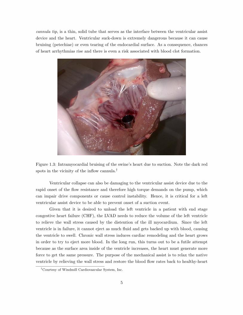
Figure 1.3: Intramyocardial bruising of the swine’s heart due to suction. Note the dark red

spots in the vicinity of the inflow cannula.†

Ventricular collapse can also be damaging to the ventricular assist device due to the

rapid onset of the flow resistance and therefore high torque demands on the pump, which

can impair drive components or cause control instability. Hence, it is critical for a left

ventricular assist device to be able to prevent onset of a suction event.

Given that it is desired to unload the left ventricle in a patient with end stage

congestive heart failure (CHF), the LVAD needs to reduce the volume of the left ventricle

to relieve the wall stress caused by the distention of the ill myocardium. Since the left

ventricle is in failure, it cannot eject as much fluid and gets backed up with blood, causing

the ventricle to swell. Chronic wall stress induces cardiac remodeling and the heart grows

in order to try to eject more blood. In the long run, this turns out to be a futile attempt

because as the surface area inside of the ventricle increases, the heart must generate more

force to get the same pressure. The purpose of the mechanical assist is to relax the native

ventricle by relieving the wall stress and restore the blood flow rates back to healthy-heart

†Courtesy of Windmill Cardiovascular System, Inc.

5

values. Consequently, heart’s need for oxygen and glucose diminishes since it has to work

less, which leads to decline in heart rate (it drops down to normal 60 beats/sec instead

of 90 beats/sec, both at rest). In order to achieve this improvement, the LVAD must

remove significant volume of blood from the left ventricle which, on the other hand, puts

the ventricular walls at risk of sucking down onto the inflow cannula. Design parameters,

such as cannula geometry, ventricular morphology, mechanical assist actuation rates and

timing, cannula insertion site, etc., all have more or less significant effects on the probability

of ventricular collapse occurring. Knowing that several of these variables are outside of the

control of the designer, ventricular suction cannot be avoided passively while maintaining

high LVAD flow rates. Therefore, it is mandatory that the LVAD system controller be able

to detect the onset of a ventricular suck-down and take different forms of action to prevent

it from becoming a damaging event.

1.4 Suction Detection Schemes

Various methods have been used to detect and prevent the onset of the suction event. Most

of the continuous flow pumps, such as DeBakey VAD, have built in flow sensors, which

are simply monitoring the amount of fluid that passes through the pump at any instant.

Decline in the quantity of fluid sends a command to the controller unit, which then takes

appropriate action to prevent a complete ventricular collapse. Some of the LVAD systems

use other types of transducers, such as pump speed (RPM counters), to detect the onset of

a suction event [23]. Voigt et al. propose a combined input from speed and current sensors

to sense the onset of a suction event [39]. However, detecting suction via sensors is often

considered insufficient, although it may not necessarily be so as we will explore in this study.

In recent years, several approaches in addition to sensory input have been used to

solve the suction detection problem. These include frequency [43] and time based [40]

methods. However, Ferreira et al. managed to combine these two approaches into one. A

proposed scheme of a suction detector consisted of frequency domain techniques which were

supplemented by a time-frequency-based feature extraction algorithm of the pump flow

signal [12]. The frequency domain indices SI1 and SI2 correspond to the fluctuation in

energy of the harmonic and subharmonic contents of the pump flow signal respectively. The

time-frequency feature extraction algorithm detects variations in the standard deviation of

instantaneous frequency of pump flow. Obviously, this method requires a flow sensor to

monitor circulation rates.

Previous algorithms often trigger off one predefined suction threshold, which de-

pends on the mechanistic features of the pump. A suction detection system that combines

multiple hemodynamic indices to produce a more reliable and robust overall suction detec-

6

tor was investigated in [2]. Because there is a great variety of suction patterns, one index

may correspond better to a certain pattern than others. Hence, the combined response to

multiple suction indices can identify a broad range of patterns compared with a detection

relying on a single index.

1.5 Motivation

The TORVAD TM left ventricular assist device is a toroidal pulsatile blood pump that has

been prototyped by Windmill Cardiovascular Systems (Austin, TX). The pumping system

is unique in that it can be synchronized to aspirate its stroke at a known time in the cardiac

cycle. This can be used to aid in the prevention of the suction phenomenon. However, as

it has been observed in many animal trials, ventricular suction cannot be avoided by this

means alone. It is therefore desired to implement a sensing mechanism to detect the onset

of suction and to take control measures, such as stopping the VAD stroke entirely, when the

beginning of the suction event is detected. Given the necessary LVAD durability, size, and

mechanical simplicity, it is undesirable to implement a flow sensor or a pressure transducer

as a part of the TORVAD TM system. A proposed method to detect suction is to monitor

the motor current signal required by TORVAD TM and use it to predict torque requirements

on the motor. Because a suction event causes a rapid rise in inflow cannula resistance, this

will manifest itself in a rapid increase in motor torque and thus current. It is hypothesized

that a suction event will present a unique current spike which can be differentiated from the

normal motor currents for the TORVAD TM system and consequently used as a threshold

to prevent a full-blown suction event.

Chapter 2 introduces both a motorized pulsatile blood pump model and a cardio-

vascular system model, as well as the connection interface model between the two. Chapter

3 describes the parametrization of the model and, therefore, ventricular collapse (suction

event) through experimental trial and error methods, bringing the model and experimental

results together. Chapter 4 explores the most widely used suction detection schemes and

focuses on the most suitable one for TORVAD TM. Using the model, Chapter 5 defines

threshold values indicative of the suction event with TORVAD TM. Additionally, the same

chapter explores different scenarios during which ventricular collapse is more or less likely

to occur and how this phenomenon affects the cardiovascular system as well as the pump.

7

Chapter 2

Model of the Pulsatile Blood

Pump, Cardiovascular System, and

Connection Interface

This chapter presents two major models: a model of the motorized pulsatile blood pump and

a model of the human cardiovascular system (CVS). The developed pump model is based

on the permanent magnet direct current (PMDC) motors. The model of the cardiovascular

system consists of the left heart and the accompanying blood vessels, and it was adopted

from the master’s thesis written by Jeffrey Gohean [15] at The University of Texas at Austin.

The two models are coupled such that physical constraints are met: the pump draws the

blood from the left ventricle and supplies it to the aorta and, therefore, the rest of the CVS.

The interface between the two systems is modeled via orifice plate equation, which is based

on Bernoulli’s Equation.

The complete system was modeled via the Bond Graph technique and simulation was

carried out in The MathWorks TM, Simulink R© software package. The bond graph notation

describes dynamical properties of systems using standard elements that are coupled with

each other with the use of power bonds. The power bond connects the ports of the elements

and indicates the energy flow through the system. More information on modeling via Bond

Graphs can be found in the literature [3, 4]. The Simulink software package is a graphical

environment for multidomain simulation and model-based design for dynamic and embedded

systems.

The complete Bond Graph model of the system is shown in Figure 2.1. Separate

Bond Graph models of the pulsatile blood pump, cardiovascular system, and the interface

between the two are shown in Figures 2.3, 2.5 and 2.9, respectively.

8

R : Rmi

1 0

1

0

Se

R : Rat

C : Cat

Prs

Pat Qat

Plv Qsa 1

R : Rsa

Δ Psa

0

C : Csa

Psa ˙ Vsa

Qoc

Vat ˙

Qao

R : Rao

Δ Pao

Qic

1

Qmi

Clv Vlv ˙ elv ˙

Sf

Δ Pmi

0 Cla Vla ˙ ela ˙

Sf

Qrs

R : Rrs 1Δ Prs

Prs

Se

Pla

Δ Pat 1

T

R : Rorice

Δ Pori

Γ I : Ic ˙

Pp

Tp

Vlv

1

: r x Ap

I : Ip

Tr

R : Rb

h ˙ G

: Km

Tm ω

Vm

i

λ

1

Vr

R : Rm

Se Vs

I : L

˙

Cardiovascular System

Connection Interface

Rotary Blood Pump

1

Pc

0 C : Cc Δ Vc ˙

Figure 2.1: Overall model diagram.

9

2.1 Model of the Motorized Pulsatile Blood Pump

The mechanism that comprises the main portion of the motorized pulsatile blood pump is

shown in Figure 2.2. It consists of a direct current (DC) motor which drives two pistons

inside of a toroidal body via two links. Only one piston moves through the toroidal chamber

at a time, while the other is stationary and rests between inlet and outlet openings.

The wound-field DC motors are usually classified as shunt-wound, series-wound, and

compound-wound. In addition to these, permanent-magnet and brushless DC motors are

also available, normally as fractional-horsepower DC motors [31]. Permanent magnet DC

motors are used in applications which require relatively low torques and economic use of

space. Because the motor under consideration is driving a low-power pump (low torque)

that is implanted into patients (small size), we will model the motorized pulsatile blood

pump as a PMDC motor, even though a practical implementation may use a brushless DC

motor.

Motor

Outlet Inlet

Piston

Figure 2.2: Toroidal pulsatile blood pump.

A PMDC motor can be modeled very effectively with just a few parameters. These

10

normally include resistive parameters such as the friction in the rotor bearings and electrical

resistance in the coil windings, inductive term due to inductance caused by coil windings,

and the gyrator coefficient of the motor. Since the pump under consideration is a positive

displacement toroidal pump, the rotational inertia of the piston is yet another significant

design parameter, along with the piston area and its distance from the rotational axis. It is

important to emphasize that the piston motion is angular and for the purpose of this thesis

follows the equation

Piston Position =

∫480

(1− cos

(2π t

Tc

))dt, (2.1)

where t is time and Tc is the duration of pump stroke (time required for piston to make one

revolution) in seconds.

The amount of fluid displaced by this pump is determined by the volume inside of

the torus (less the piston volumes) and is given by

Stroke V olume = ApCt , (2.2)

where Ap is the piston area and Ct is the circumference of the torus.

1Se :V

i

R:R

mVri

I:L

λi

GYKm

Vm

i

τm

ω 1

R:R

bτrω

I:Ip

hω

TFr × Apτp

ω

Pp

Q

Figure 2.3: Toroidal blood pump Bond Graph.

State equations describing the dynamics of the pump in terms of flux linkage λ and

angular momentum h are outlined in equations (2.3) and (2.4), respectively. Position of the

rotor is monitored through an information state θ (equation (2.5)), which is being detected

11

by an angular-velocity to angular-position sensor model. The desired piston position, also

termed tracking curve, is controlled via proportional-integral-derivative (PID) controller.

Note that the control variable is the supply voltage V , where a power supply of about 14V

is assumed available. Thus, in this model, saturation limits impose upper and lower bounds

on input signals in order to suppress unlimited draw of power.

λ = V − Rm

Lλ− Km

Iph (2.3)

h =Km

Lλ− Rb

Iph− rApPp (2.4)

θ =

∫ω(t) dt =

∫1

Iph(t) dt (2.5)

The values used in this model, shown in Table 2.1, were adopted from the left

ventricular assist device called TORVAD TM, prototyped by the accompany named Windmill

Cardiovascular Systems based in Austin, TX.

Motor Parameter Symbol Value Units

Supply Voltage V 10− 14 V

Gyrator Coefficient Km 0.124 V secrad

Two Phases in Series Resistance Rm 2.6 Ω

Damping Coefficient Rb 8.1× 10−5 Nmsecrad

Two Phases in Series Inductance L 2.58× 10−3 H

Inertia of the Rotating Piston Ip 1.851× 10−5 kgm2

Area of the Piston Ap 2× 10−4 m2

Distance from the Rotation Axis r 0.03 m

Stroke Volume ∀s 37.6 ml

Table 2.1: Typical PMDC parameter values used for simulation in this thesis.

12

2.2 Model of the Cardiovascular System

Several comprehensive models of the cardiovascular systems have been developed in recent

years [1, 15, 18]. Gohean developed a computational model specifically to study the effect

of mechanical assist devices on the cardiovascular system [15]. Both the systemic and

pulmonary circulation have been modeled to complete the loop around the area of focus,

namely the aorta and large arteries. This thesis however, adopts only the model of the left

heart (left ventricle and left atrium), along with the accompanying left heart valves (mitral

and aortic), and the systemic circulation (arteries and arterial tree) from Gohean’s work.

As the left heart comprises the biggest portion of the myocardial muscle, and since LVADs

are connected to the heart at the left ventricular apex site, the adopted portion of Gohean’s

model appears sufficient to study ventricular collapse.

Pulmonary Circulation

Systemic Circulation

Arterioles

Capillaries

Arteries

Veins

Veins

Heart

Valve

Arteries

ArteriolesCapillaries

LA LV

RV RA

C ( t)

A

B B

B

BB

1

23

4 6

57

9

10111213

14 15 B1617

18 B1920 20

2121

22B22

B B24 24

23 23

8

BB

BB

B

x

yz

p

α β

1

αβαβ

β

β

αβ

α

α

α

α β α β

2

3

4

α β3

α β3

22

2

3

2

αβ2

Figure 2.4: Cardiovascular system schematic, from [15]. Only left heart along with the

systemic circulation has been adopted (marked in red).

The model is shown in Figure 2.5 in terms of Bond Graph modeling technique.

Detailed description of the model, including parameters and ordinary differential equations,

is outlined in Appendix A.

13

R : Rmi

1 0

1

0

Se

R : Rat

C : Cat

Torvad

Prs

Pat Qat

Plv Qsa 1

R : Rsa

Δ Psa

0

C : Csa

Psa ˙ Vsa

Qoc

Vat ˙

Qao

R : Rao

Δ Pao

Qic

1

Qmi

Clv Vlv ˙ elv ˙

Sf

Δ Pmi

0 Cla Vla ˙ ela ˙

Sf

Qrs

R : Rrs 1Δ Prs

Prs

Se

Pla

Δ Pat TM

Figure 2.5: Cardiovascular system Bond Graph.

Subscript Definition

rs Right side pulmonary venous return

la Left atrial

mi Mitral

lv Left ventricular

ao Aortic

ic Inlet cannula

oc Outlet cannula

sa Systemic arteries

at Arterial tree

Table 2.2: Subscript definitions for the cardiovascular system Bond Graph.

14

2.3 Model of the Pump-CVS Interface

Patients suffering from congestive heart failure (CHF) often receive mechanical assists as

a bridge to real heart transplantation or as a method of therapy under which the heart

undergoes remodeling to its original shape. A mechanical assist device is interfaced to

the ventricular chamber via cannula. Most often, the left ventricular apex is chosen as

the site for pump cannula tip insertion. One such cannula tip was designed by Windmill

Cardiovascular Systems and is employed with the TORVAD TM left ventricular assist device.

Note that the cannula tip shown in Figure 2.6 is made out of plastic material for the research

purposes. Clinical cannula tips have identical geometry, albeit made out of steel. The

cannula tip shown was fabricated only for in vitro testing.

Figure 2.6: Inflow tip, designed by Windmill CVS.

Ventricle-to-pump fluid coupling losses can be modeled via orifice flow relations.

Namely, the flow from the heart can be modeled similar to the flow from a pipe with large

diameter relative to an orifice. As fluid flows through this pipe, it encounters a narrow

section and it is forced to converge. Pressure and velocity change as a consequence of a

change in flow area [26]. It turns out that the pressure at point (1) in the figure below is

larger than at point (2) within the vena contracta (the point in a fluid stream where the

diameter of the stream is the smallest).

15

Figure 2.7: Fluid flow through orifice, from [26].

In the absence of viscous effects, Bernoulli’s equation can be applied at two points

on the streamline which passes through the middle of the interface:

P1 +1

2ρV1

2 + ρgz1 = P2 +1

2ρV2

2 + ρgz2 , (2.6)

where P is the thermodynamic pressure of the fluid as it flows (sometimes termed as static

pressure), 12ρV

2 is the dynamic pressure, and ρgz is the hydrostatic pressure, due to po-

tential energy variations of the fluid as a result of change in elevation [26]. Under the

assumption of a horizontal setup (no change in elevation), hydrostatic pressure terms can-

cel out in Bernoulli’s equation, which then simplifies to

∆Pori =1

2ρV2

2 − 1

2ρV1

2 , (2.7)

where ∆Pori = P1 − P2 is the pressure across the orifice. Based on the fluid dynamics laws

of conservations, which are expressed using the Reynolds Transport Theorem, the mass and

therefore the flow is conserved inside of the pipe:

Q = A1V1 = A2V2 ⇒ V1 =A2V2A1

, (2.8)

where A1, A2 and V1, V2 are cross sectional areas and velocities at points (1) and (2).

Substituting V1 into equation (2.7), and solving for velocity at point (2) we get

V2 =

√2(∆Pori)

ρ(1− β4), (2.9)

where β = D2/D1 (ratio of the diameters at points 1 and 2). Note that non ideal effects

occur for a couple of reasons: 1) vena contracta area A2 is less than the area of the orifice

Ao by some percentage (A2 = CcAo) and 2) turbulent flow near the cannula introduces a

16

loss which cannot be calculated theoretically. Hence, an orifice discharge coefficient, Cd is

used to accommodate for these phenomena. The equation (2.8) finally becomes

Q = CdAo

√2(∆Pori)

ρ(1− β4), (2.10)

where Ao = πd2/4 (refer to figure 2.7). It is important to realize that Cd is a function of

β = d/D and Reynolds number Re = ρV D/µ, where V = Q/A1. Nominal values of Cd

are in the vicinity of 0.6; however, they also depend on the geometry of the orifice plate

(cannula), whether the edges are beveled or sharp on the cannula, placement of pressure

taps etc. Thus, it is usually necessary to experimentally determine the value of the discharge

coefficient Cd for cannula in order to parameterize this model accurately.

The pressure versus flow curve shown in Figure 2.8 was obtained via the experimental

setup outlined in Section 3.2 of Chapter 3. Note the quadratic relationship between pressure

and flow rate (P α Q2), confirming equation (2.10). The value of the discharge coefficient

Cd that brings the pressure values across the cannula in the model closer to the values

obtained experimentally (Figure 2.8) is 0.35. Note that this value was acquired for plain

tap water at room temperature.

2 4 6 8 1 0 1 2

0 . 0 0

0 . 0 5

0 . 1 0

0 . 1 5

0 . 2 0

O r i f i c e P l a t e F i t C u r v e

Pressu

re (PS

I)

F l o w ( L / m i n )

Model PolynomialAdj. R-Square 0.99979

Value Standard ErrorPressure Intercept -0.00166 0.00165Pressure B1 -7.17656E-4 5.67877E-4Pressure B2 0.00176 4.28785E-5y = Intercept + B1*x^1 + B2*x^2

Figure 2.8: Pressure vs. Flow across orifice.

17

1 0

Qoc = Qp

Qic

Clv

1 R : Rorice

Δ Pori

Γ I : Ic ˙

Pp

Vlv

: r x Ap

1

Pc

0 C : Cc Δ Vc ˙

Figure 2.9: Bond graph model of the pump-CVS junction.

The model of the rest of the coupling interface in terms of Bond Graphs is shown

in Figure 2.9. Apart from including the pressure drop across the orifice, an inertance term

due to the momentum of the fluid in the cannula and tubing connections has been added.

The fluid inertance is estimated by the following equation:

Ic =ρL

Ac, (2.11)

where L is the length of the pipe in general (assumed value of 0.5m) and Ac is the cross

sectional area of the pipe (cannula) with the diameter of 0.0185m. Note that the causal

stroke on the Bond Graph for this I element indicates the derivative causality (away from

the effort junction 1), making the in fluid momentum Γ a dependent variable. This means

that no extra state describing additional dynamics of the system is required.

18

Qoc

Qic

R L

Figure 2.10: Model of the elastic tube.

Besides the inertia of the fluid that is developed as the fluid flows through the

cannula, the elastic effect of the cannula itself was modeled. Namely, for an incompressible

fluid, we can determine the expression for the capacitance of the tube’s elastic effects, since

the tube expands. After the expansion, the area of the cannula is

Af = πR2f = π(R+ ∆R)2 = πR2 + 2πR∆R+ π(∆R)2 , (2.12)

where R is the original radius and ∆R is the change in the original radius. ∆R, which

represents expansion in the radial direction, can be approximated from formulas for stress

and strain [42], yielding

∆R =PR2

Et(1− ν

2) , (2.13)

where P is external pressure, E is Young’s elastic modulus of the cannula material, t is

the thickness of the cannula, and ν is Poisson’s ratio of the cannula material. In reality,

the inlet cannula may be made from a material such as expanded polytetrafluoroethylene

(ePTFE), which is completely inert and extremely biocompatible; the body does not reject

parts made out of this material.

Parameter Definition Value

L Cannula length 0.5m

t Cannula thickness 0.003m

R Cannula radius 0.0184m

E ePTFE Young’s modulus 0.5GPa

ν ePTFE Poisson’s ratio 0.46

Table 2.3: Relevant design parameter for the inlet cannula.

19

Neglecting the last term on first approximation, equation (2.12) reduces to

Af = πR2 + 2πR∆R = A+ ∆A. (2.14)

Therefore, the volume change due to tube expansion is

V ∼= (∆A)L = 2πRR2L

Et(1− ν

2)P. (2.15)

Recognizing the original volume term of the cannula (Vo = πR2L) in the above

expression we can rewrite the above equation as

V =2VoR

Et(1− ν

2)P ⇒ P =

1

CcV , (2.16)

where Cc is the elastic compliance for expansion∗ of the cannula used in the model

Cc =2VoR

Et(1− ν

2). (2.17)

Sources of effort such as Plv, Psa, and Pp are defined from the cardiovascular system

model and the model of the toroidal pulsatile pump, respectively. Inflow cannula flow Qic

and outflow cannula flow Qoc dictate the change of volume inside of the elastic canula.

Outflow cannula flow Qoc is equal to that of the pump Qp since no elastic effects were

modeled inside the pump.

2.4 Initial Verification of the Model

This section shows several test cases that verify the functionality of the base model. One

way to verify the model is to plot so called PV Loops of the patient data and the model,

and hence investigate how they compare. Left ventricular pressure-volume (PV) loops are

derived from pressure and volume values found in the cardiac cycle. To generate a PV loop

for the left ventricle, the left ventricular pressure is plotted against left ventricular volume

at multiple time points during a complete cardiac cycle.

∗Note that a different compliance could be required for collapse of the cannula.

20

Figure 2.11: A case study of measured LV pressure, volume and wall thickness during a

cardiac cycle of a healthy person (left). Relationship between LV volume and pressure

(right).

Figure 2.11 shows an example of a patient’s measured LV pressure, volume and wall

thickness during a cardiac cycle. Looking at the right portion of the above figure, points

21-36 constitute the blood filling phase, 1-5 constitute the isovolumic contraction phase, 5-

17 constitute the blood ejection phase, and 17-21 constitute the isovolumic left ventricular

relaxation phase [44, 45].

0 20 40 60 80 100 120 140 1600

20

40

60

80

100

120

140

160

V(mL)

P(m

mH

g)

Figure 2.12: PV Loop obtained via cardiovascular system model

21

Figure 2.12 shows the plot of several cardiovascular cycles (heart beats) of the healthy

left ventricle. Note that the blue lines eventually start to overlap, signaling that the model

has reached a steady state. On average, ventricular volume is at 110ml (vertical line through

the middle of the PV Loop) and the average left ventricular pressure is about 80mmHg

(horizontal line through the middle of the PV Loop), which is very similar to the values

on the previous page. The volume of the blood that gets ejected with each heart beat is

contained within two vertical isovolumic lines, and this value is 70ml on average.

0 50 100 1500

20

40

60

80

100

120

140

160

180

V(mL)

P(m

mH

g)

Figure 2.13: PV Loop obtained via cardiovascular system model, with pump attached

Figure 2.13 shows how the overall model performs with the model of a toroidal

pulsatile blood pump attached to the cardiovascular system model. Note that the volume

of the left ventricle is constantly changing as we go around the PV loop (slanted vertical

lines). This means that there is no isovolumic period during the cardiac cycle; rather the

pump is altering the left ventricular volume constantly as it actuates along with the heart.

Now that we have verified that the joint model of the pump, cardiovascular system

and the interface between them works, we will go ahead and attempt to model ventricular

collapse. The phenomenon of the ventricular suck-down will be superimposed on top of the

base model described in this chapter.

22

Chapter 3

Experimental Suction

Parameterization: Variable Orifice

Resistance

The model described in Chapter 2 has been further parameterized in this chapter to simulate

suction event dynamics inside of the left ventricle. The suction event has been superimposed

onto the base model described earlier. This chapter describes the process of obtaining

relevant parameters that would enable modeling and simulating suction events. The chapter

includes a section on development of a physical approximation of the left ventricle as well

as a section on experimental estimation of ventricular collapse using data from testing with

an artificial left ventricle and a mock circulatory loop.

3.1 Ellipsoidal Approximation of the Left Ventricle

Left ventricle shape and hence the volume is often approximated via ellipsoid [32, 33].

Volume of an ellipsoid is given by

V =4

3πabc,

where a, b and c are elliptic radii.

Assuming that two of the radii are same and that the LV appears as half of an

ellipsoid, the above equation becomes

V =4

6πab2. (3.1)

Equation (3.1) was used to design an artificial left ventricle, along with the LV ge-

23

ometry data obtained from the literature. Taking into account end diastolic left ventricular

volume of a healthy person, atrioventricular plane to heart apex distance (long axis), diame-

ter of the left ventricle (short axis distance) and the ventricular wall thickness, the following

3D model was developed in SolidWorks CAD design software:

(a) (b)

Parameter Value

Volume (ml) 120∗

Long Axis (mm) 84†

Short Axes (mm) 26.12‡

Wall Thickness (mm) 12∗

Interface Length (mm) 50.8§

(c)

Figure 3.1: LV computer aided design: (a) Triangle edges; (b) Shaded; (c) Dimensions.

3.1.1 LV Rapid Prototyping and LV Silicon Mold

Rapid prototyping (RP), a fast turnaround additive manufacturing technology, was used

to fabricate the part shown in Figure 3.1. Once the SolidWorks part was developed and

converted into RP machine readable format, the file was submitted for manufacturing.

The end product of this process was a rigid left ventricle shown in Figure 3.2. Next,

this rigid part was used to create a two-part silicon mold, which on the other side was meant

∗Values from [13, 9]†Values from [34]‡Value determined from eq. 3.1, by specifying LV volume and long axis radius§Cylindrically shaped mock loop interface of length L = 50.8mm (2in) was added to the ellipsoid

24

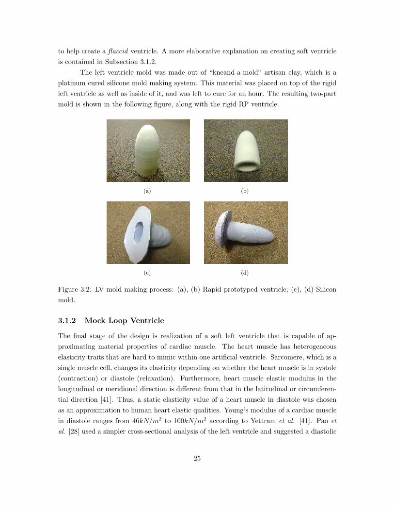
to help create a flaccid ventricle. A more elaborative explanation on creating soft ventricle

is contained in Subsection 3.1.2.

The left ventricle mold was made out of “kneand-a-mold” artisan clay, which is a

platinum cured silicone mold making system. This material was placed on top of the rigid

left ventricle as well as inside of it, and was left to cure for an hour. The resulting two-part

mold is shown in the following figure, along with the rigid RP ventricle.

(a) (b)

(c) (d)

Figure 3.2: LV mold making process: (a), (b) Rapid prototyped ventricle; (c), (d) Silicon

mold.

3.1.2 Mock Loop Ventricle

The final stage of the design is realization of a soft left ventricle that is capable of ap-

proximating material properties of cardiac muscle. The heart muscle has heterogeneous

elasticity traits that are hard to mimic within one artificial ventricle. Sarcomere, which is a

single muscle cell, changes its elasticity depending on whether the heart muscle is in systole

(contraction) or diastole (relaxation). Furthermore, heart muscle elastic modulus in the

longitudinal or meridional direction is different from that in the latitudinal or circumferen-

tial direction [41]. Thus, a static elasticity value of a heart muscle in diastole was chosen

as an approximation to human heart elastic qualities. Young’s modulus of a cardiac muscle

in diastole ranges from 46kN/m2 to 100kN/m2 according to Yettram et al. [41]. Pao et

al. [28] used a simpler cross-sectional analysis of the left ventricle and suggested a diastolic

25

value of 92kN/m2.

In order to achieve the above mentioned values for left ventricular Young’s modulus,

arbitrary heart-like elastic materials were tried. Among others, polyvinyl chloride with

phthalate plasticizer, often termed as plastisol, seemed to satisfy the requirements. Plastisol

is a white, milk-like base to which softeners and hardeners can be added to achieve desired

stretchiness and/or stiffness. The cure time for plastisol is temperature dependent: the

higher the temperature, the faster the cure¶. Hot material can be poured into molds and

left to cool down to room temperature. A Collapsible left ventricle is shown in Figure 3.3.

(a) (b)

Figure 3.3: Mock loop left ventricle: (a) Supine position and (b) Standing position.

Several different ratios of the base material and softener were tried until cured plas-

tisol Young’s modulus matched that of a heart in diastole. Experimental procedures showed

that four parts of plastisol base P0010RB to one part of softener RD-55 achieved Young’s

modulus of 72.6kN/m2 on average, which falls within the range found in the literature

for diastolic elasticity values. Recall that the slope of the stress versus strain curve is the

Young’s modulus of elasticity:

E ≡ tensile stress

tensile strain=σ

ε=

F/A0

∆L/L0=

FL0

A0∆L

where,

• E is the Young’s modulus (modulus of elasticity)

• F is the force applied to the object

• A0 is the original cross-sectional area through which the force is applied

• L is the amount by which the length of the object changes

• L0 is the original length of the object.

¶Manufacturer (QCM COMPANY INC.) does not recommend going above 380-400 F as that can resultin burned plastisol

26

3.2 Experimental Estimation of Flow Characteristics during

Ventricular Collapse via Mock Circulatory Loop

Parametrization of flow characteristics during a suction event was done experimentally with

the aid of mock circulatory loop. Mock circulation loops are generally used to evaluate the

performance of cardiac assist devices prior to animal and clinical testing [16]. A compress-

ible, translucent plastisol chamber that mimics the size, shape and motion of a left ventricle

is desired to assist in pressure/flow studies around inflow cannula during VAD support.

The aim of this study was therefore to design and construct a mock circulation loop with a

naturally shaped flexible left ventricle and evaluate its performance during suction events.

The data extracted during this series of experiments was used to parametrize the

model outlined in the previous chapter in order to study effects of ventricular collapse on

the mechanical assist device and human cardiovascular system.

Figure 3.4: Mock loop schematic.‖

Yuhki et al. [43] have performed studies with the mock circulatory loop and artificial

silicon ventricle in order to study ventricular collapse. In particular, intention was to detect

suction and flow regurgitation based on the motor current waveform so that pump operation

mode can be optimized and patient saved from potential suffering. Similar mock loops were

developed by others though for different purposes. Cassot et al. [6] developed a physical

model to simulate left heart and systemic circulation. In addition, they wanted to visualize

‖Components of the loop are not drawn to scale.

27

flow patterns inside of the ventricle at the early filling stage as well as at the onset of

ventricular systole. Pantalos et al. [27] saw mock circulation fit to test mechanical assist

devices for healthy and pathological states. They argued that in vitro studies via these

loops should be well suited for developing experimental protocols, testing device feedback

control algorithms, investigating flow profiles, and training surgical staff on the operational

procedures of cardiovascular devices.

Majority of these loops consist of a combination of the following components:

• pneumatically driven artificial left ventricle

• mechanical assist device

• pressure, flow, velocimeter sensors

• visualization aids (dye, scope, cameras)

• arterial/aortic compliance chamber

• tubing of certain length

• restrictions to flow simulating resistance,

and the outline of the ones used to parametrize the ventricular collapse in this study is

shown in Figure 3.5.

28

(a)

# Item

1 Instrumentation amplifier

2 Power Supply 1

3 Power Supply 2

4 Oscilloscope

5 Biomedicus pump

6 Flow Probe

7 Differential pressure sensor

8 Inflow cannula

9 Artificial ventricle

10 Pressure resorvoire

(b)

Figure 3.5: Mock circulatory loop: (a) Experimental setup and (b) Components.

29

The Medtronic bio-pump called BioMedicus is a centrifugal blood pump used for

extracorporeal circulatory support for patients under cardiopulmonary bypass (a technique

which temporarily substitutes the function of the heart and lungs during surgical procedure).

The pump impeller has a series of smooth-surfaced rotating cones which pull the blood into

the vortex created by the rotation, after which the blood is propelled out of the system.

The flow probe TX-40 comes factory calibrated and interfaces through a connector to the

control console.

Figure 3.6: Bimedicus centrifugal blood pump and the flow probe.

A differential pressure sensor (OMEGAs PX26-001DV) was placed across the cannula

tip since the pressure change should manifest itself at this site at the moment of ventricular

suck-down. The PVC cannula tip that is inserted into the artificial ventricle reflects the

pristine design of the steel tip utilized with TORVAD TM, left ventricular assist device

prototyped by Windmill Cardiovascular Systems, Inc.

Figure 3.7: Differential wet-to-wet pressure transducer placed across cannula tip.

30

Figure 3.8: Experimental suction parametrization: Measurements were taken while the

volume of the left ventricle was varied with the clamp.

0 2 4 6 8 1 0 1 20 . 0

0 . 1

0 . 2

0 . 3

0 . 4

0 . 5 L V V o l u m e = 1 2 0 m l L V V o l u m e = 9 6 m l L V V o l u m e = 7 2 m l L V V o l u m e = 4 8 m l L V V o l u m e = 2 4 m l L V V o l u m e = 1 0 m l

Pressu

re (ps

i)

F L o w ( L / m i n )Figure 3.9: Experimental suction parametrization : P vs. Q. Resistance value (flow coeffi-

cient) increases as the ventricle collapses.

31

0 . 0 0 0 0 0 0 . 0 0 0 0 4 0 . 0 0 0 0 8 0 . 0 0 0 1 20 . 0 0 E + 0 0 0

1 . 0 0 E + 0 1 0

2 . 0 0 E + 0 1 0

3 . 0 0 E + 0 1 0

4 . 0 0 E + 0 1 0

5 . 0 0 E + 0 1 0

6 . 0 0 E + 0 1 0 R e s i s t a n c e E x p o n e n t i a l F i t o f R e s i s t a n c e

Resis

tance

(Pa m

3 )/sec

L V V o l u m e ( m 3 )

Equation y = y0 + A*exp(R0*x)Adj. R-Square 0.88535

Value Standard ErrorResistance y0 3.3267E10 5.52756E9Resistance A 4.56144E10 7.75395E9Resistance R0 -28689.58334 14619.71142

Figure 3.10: Experimental suction parametrization: Rorifice vs. Vlv obtained from figure

3.9.

Dependency of the resistance (flow coefficient) on the left ventricular volume is ex-

pressed in equation (3.2). This relation is used to modulate resistance values across the

cannula interface during ventricular collapse (Figures 2.1 and 2.9, connection interface sec-

tion). Implementation of the volume-based resistance brought together experimental results

and the Simulink model.

Rorifice = 3.26E10 + 4.56E10e−28689.6Vlv (3.2)

The above expression was used as a means of inducing ventricular suction event in

the model. The following chapter will get the reader familiarized with a suction detection

algorithm proposed for detecting the onset of a ventricular collapse.

32

Chapter 4

Suction Detection Algorithm

This chapter investigates suction detection schemes and focuses on the most plausible one

based on the mechanistic features of the TORVAD TM system and experience of engineers

working at Windmill Cardiovascular Systems, Inc.

Suction has been investigated for pumps involved in heavy industry applications such

as sewage systems, water supply networks etc., in order to prevent malfunctioning of the

pumping mechanisms due to clogging [35]. In addition, occurrence of suction phenomenon

and its detection has been studied in left ventricular assist devices [2, 12, 23, 39, 40, 43], as

outlined in the introductory chapter, Section 1.4. It is important to understand implications

of the suction phenomenon well in order to be able to approach and solve the problem

appropriately. For instance, its occurrence is highly undesirable, even for short periods of

time for it can induce high torque demands and damage the pump system performance,

causing instability problems. More importantly, suction events can leave petechia (bruises)

on the ventricle walls and interventricular septum (the wall separating the left and right

ventricles of the heart). Occurrence of ventricular suck-down can also induce tachycardia,

which is a heart rate that exceeds the normal range for a resting heart beat [36].

Multiple, readily available signals can be used as indices of an imminent suction

event. Variations in the flow, speed, current, and power waveforms (or their combination)

are often employed as mechanisms to detect the onset and/or presence of ventricular col-

lapse. Processing and analysis of these inherent pump system parameters can be done in

time [40] and frequency domains [43]. Time domain mechanisms include correlation tech-

niques as well as linear and non-linear signal processing. Frequency domain mechanisms

include various real-time spectral analysis methods using different kinds of Fourier Trans-

forms (FFTs and DFTs), as well as other linear and non-linear signal processing techniques.

Section 4.1 of this chapter introduces some commonly used suction detection schemes

for LVADs in general. Section 4.2 focuses on arguably the most suitable suction detection

33

algorithm for TORVAD TM left ventricular assist device.

4.1 Detection Methods

An extensive list of suction detection schemes is outlined in the patent called Method and

System for Detecting Ventricular Collapse [25]. We will go through few items on this list

and present advantages and disadvantages of each method, in an attempt to identify the

most viable one for a positive displacement toroidal pump, such as the TORVAD TM.

4.1.1 Sensory Input Alone

In certain designs, such as the DeBakey LVAD, the flow signal provided via the flow sensor or

flow meter is specifically analyzed for suction detection. Monitoring the flow rates through

the pump is considered an acceptable method of detecting suction, although not the most

assuring one. In addition to only one sensory input, a combination of several of these signals

such as motor current, power and speed may be used to avoid false positives for instance.

However, this means alone (via sensors) is often considered insufficient, and additional signal

processing is used to get positive triggers when suction event occurs.

4.1.2 Harmonic Distortion Analysis of a Signal

Fluctuations in the flow, speed, current, and power signals in the time-domain will result in

corresponding variation in their frequency-domain representations. Thus, real time spectral

content information of these signals may be used to detect ventricular collapse. Several

kinds of suction indices can be generated based on harmonic spectral analysis:

i) harmonic distortion

ii) total spectral distortion (harmonic distortion and noise)

iii) sub-fundamental distortion (distortion below the fundamental frequency)

iv) super-fundamental distortion (distortion above the fundamental frequency)

v) the ratio of the super-fundamental distortion to the sub-fundamental distortion

vi) super-physiologic distortion (distortion at frequencies above the assumed maximum

physiologic fundamental frequency-typically 4 Hz or 240 BPM)

vii) and the spectral dispersion or “width” of the resulting flow waveform.

The potential drawback of this method is that it can be computationally expensive. Onset

of a suction event may go undetected if the controller is not fast enough and does not have

digital signal processing (DSP) capabilities. This method also poses an issue of defining

34

what is meant by a real-time frequency spectrum of a signal. Again, we find an answer

by determining how fast a micro-controller can execute all the operations and produce a

probability index of the suction event in a timely fashion, preventing a complete ventricular

collapse.

4.1.3 Spectral/Time Domain Masking

In addition to spectral harmonic indices previously described, spectral content of the mea-

sured signal may be used differently to detect onset of a suction event. Essentially, the

spectral content generated by the FFT is compared to a predetermined spectral mask.

Hence, the presence of a suction event is determined based on the comparison. The signals

whose spectral components fall within the mask indicate suction and, conversely, signals

whose spectral components fall outside the mask indicate normal operating conditions.

A similar approach can be used for time domain analysis methods. A particular

method cross-correlates the incoming time-sampled signal (for example, the flow or cur-

rent signal) with predetermined time-domain waveforms which exemplify the imminence of

ventricular suck-down. The mask waveforms are selected sequentially or are based on the

probability of occurrence in that particular patient derived experientially through clinical

evaluation. A correlation coefficient signifies a perfect match or indicates no correlation at

all. The correlation coefficient is compared to predetermined thresholds to derive a suction

probability index. If the calculated correlation coefficient exceeds a predetermined value,

ventricular collapse is imminent. Conversely, if the calculated correlation coefficient is below

the predetermined value, suction is not present.

Drawbacks of the spectral masking method are identical to the Harmonic Distortion

Analysis method, that is, a lack of micro-controller computational power may produce non-

real-time triggers. A time domain approach relies on experimentally determined masks

that are obtained via clinical evaluation of patients. Given that mechanical assist devices

go through rigorous animal trials before they are approved for clinical usage in patients,

this method may not be the most appropriate, since suction detection should be operational

from the moment a patient receives an implant.

4.2 Suction Detection for TORVAD TM

The TORVAD TM left ventricular assist device is a pulsatile positive displacement toroidal

blood pump. The algorithm under consideration was derived based on the mechanistic

features of the TORAVD system and computational abilities of the micro-controller unit.

As it was described earlier, suction detection schemes need some kind of a sensory input

35

(flow, current, speed etc.) and some sort of a processing algorithm that behaves in a robust

manner.

The TORVAD TM ventricular assist device provides two types of inherently available

signals: a) piston position (and therefore velocity) and b) current magnitudes, which are

closely related to the amount of torque inquired by the pump due to the change in load.

The proposed scheme consists of two steps:

1. The current signal may be combined with motor position error as a means for imple-

menting the needed motor action to prevent further suction.

2. Additional signal analysis is desired as a means of providing not only algorithm re-

dundancy but also supplementary suction event thresholds. The time derivative of

the pump’s current i can be calculated and used as an extra precaution:

di(t)

dt=−i(to + 2∆t) + 8i(to + ∆t)− 8i(to −∆t) + i(to − 2∆t)

12∆t+ ϑ(∆t)4 (4.1)

In numerical analysis, given a line grid in one dimension, the five-point stencil of a

point in the grid is made up of the point itself together with its two adjacent neighbors on

each side. It is used to write finite difference approximations to derivatives at grid points.

Note that the above formula is fourth order in accuracy ϑ(∆t)4, and that it follows from

the Taylor’s Series expansion around the central point [11]. Time step ∆t is defined as a

reciprocal of the sampling frequency fs.

36

Chapter 5

Results

Having made a base model in Chapter 2 (the pump, cardiovascular system and the can-

nula/tube interface) and experimentally parametrized suction flow characteristics in Chap-

ter 3, with a suction detection algorithm (Chapter 4) we proceed into evaluating how these

three systems interact with each other. This chapter presents several test cases that were

used to investigate likeliness of a suction event occurrence, and evaluate suction detection

algorithm. In addition, this chapter describes examples of suction events obtained during

animal trials with TORVAD TM and compares those to the ones obtained from simulations.

Lastly, the chapter also depicts how ventricular collapse affects the cardiovascular system

as well as the pump.

5.1 Defining Thresholds

The following figures compare the regular mode of operation of the model against the in

vivo animal trial data, for verification purpose. Suction thresholds were determined based

on the figures presented in this section and they indicate the onset of a suction event.

It is hypothesized that suction events will produce higher torque demands on the motor

than usual during ventricular collapse, which, by virtue of how the motor operates, will

require higher draw of power, manifested in the sudden current increase. Hence, based on

the observation of Figure 5.1 we can safely note that normal mode of operation does not

require current amplitudes higher then approximately 0.7 amperes for the model, and 0.6

amperes for the animal trial case.

37

0 . 0 0 0 . 7 5 1 . 5 0 2 . 2 5 3 . 0 0 3 . 7 50 . 0

0 . 2

0 . 4

0 . 6

0 . 8

1 . 0

t ( s e c )

Curre

nt (Am

p)

0

3 6 0

7 2 0

1 0 8 0

1 4 4 0

1 8 0 0

Piston

Positi

on (D

eg)

(a)

2 4 2 6 2 8 3 00 . 0 0

0 . 2 5

0 . 5 0

0 . 7 5

1 . 0 0

t ( s e c )

Curre

nt (Am

p)

0

1 0 0 0

2 0 0 0

3 0 0 0

4 0 0 0

Piston

Positi

on

(b)

Figure 5.1: Pump current and piston position, no suction: (a) Model; (b) In vivo. Note

that in vivo piston position is sampled with a Hall sensor and that sampled values go to

zero after each piston cycle. The piston in the model follows a smooth tracking curve, which

must not go to zero, for this sudden discontinuity would induce a back flow in the model.

Current derivative thresholds on the other end differ significantly, mainly due to

imperfections of the model (Figure 5.2). Nonetheless, applying a 5-point-stencil numerical

derivative (Chapter 4) to both the model and the animal trial data, we obtain the following

threshold values: approximately 5 for the model and approximately 10 for the iv vivo case.

0 2 4- 1 0 . 0

- 7 . 5

- 5 . 0

- 2 . 5

0 . 0

2 . 5

5 . 0

7 . 5

1 0 . 0

Curre

nt De

rivati

ve

t ( s e c )

(a)

0 3 6 9- 1 5

- 1 0

- 5

0

5

1 0

1 5

Curre

nt De

rivati

ve

t ( s e c )

(b)

Figure 5.2: Pump current derivative, no suction: (a) Model (b) In vivo.

In the next section, we will introduce a suction event into the model in order to see by

how much the above defined thresholds deviate, if at all. It is speculated that monitoring

38

these thresholds only, that is current and its rate of change, is sufficient to detect the

ventricular collapse.

5.2 Suction Event

Typical instance of a suction event, which occurred during an animal trial conducted by

Windmill Cardiovascular Systems is shown in Figure 5.3. The model predicts an increase in

current values. Note that the base threshold value of 0.5 amperes, which we have previously

defined, was exceeded significantly in both the model and reality. In addition, derivative

thresholds have been surmounted in both instances; however, the maximum indices differ

significantly. This should not pose a problem, as we are only interested in tracking no-

suction values and taking controller action when these are exceeded.

0 2 40

2

4

6

8

1 0

Curre

nt (Am

p)

t ( s e c )

(a)

0 1 0 2 0 3 00 . 0

0 . 5

1 . 0

1 . 5

2 . 0

2 . 5

3 . 0

3 . 5

4 . 0

Curre

nt (Am

p)

t ( s e c )

(b)

0 1 2 3 4- 4 0 0

- 2 0 0

0

2 0 0

4 0 0

6 0 0

Curre

nt De

rivati

ve

t ( s e c )

(c)

0 1 0 2 0 3 0

- 8 0

0

8 0

Curre

nt De

rivati

ve

t ( s e c )

(d)

Figure 5.3: (a) Pump current from the model and (b) pump current sampled during animal

trials. (c) Pump current derivative from the model and (d) pump current derivative

calculated from animal trial data. Few aspiration cycles are shown along with the suction

event occurring, and later declining.

39

5.2.1 Suction Event Effects on CVS

Now that the suction indices have been defined for both the current and its rate of change,

and further verified/compared with the animal trial data, we will investigate what physio-

logical effects suction events could possibly have on the cardiovascular system. Note that

there is no available physiological data from the animal trials that we can compare output

of the model against. Therefore, the model will be used to provide us with insights into

physiological consequences, while investigating different modes of operation of the pump,

which is virtually impossible during animal trials and especially patient trials.

A suction event induces ventricular collapse. This phenomenon is most likely to

occur just at the cannula insertion site as it was explained in the introductory chapter and

shown in Figure 1.3. Tracking left ventricular volume during the model simulation gives

insights into suction event occurrence. Yet, a better way of visualizing suction event can be

achieved by tracking the left ventricular diameter:

d =

√6VlvLπ

, (5.1)

where L is the longitudinal radius of the ellipsoid. Recall that the left ventricular shape

and therefore the volume can be estimated with a half ellipsoid (equation (3.1)). Knowing

that the average distance from the atrio-ventricular plane to ventricular apex is L = 8.4cm

and having the state variable Vlv readily available at every time step during simulation, we

can estimate how the ventricular diameter changes at the atrio-ventricular plane, i.e. short

axis diameter of the ellipsoid.

40

0 2 40

1

2

3

4

5

6

7Le

ft ve

ntric

le d

iam

eter

(cm

)

t (sec)

(a)

0 2 40

1

2

3

4

5

6

7

Left v

entric

le dia

meter

(cm)

t ( s e c )

(b)

Figure 5.4: Left ventricle short axis diameter, approximated at the atrio-ventricular plane:

(a) Suction and (b) Normal. Values in the graph for suction case are below the range found

in the literature for the normal end systolic and end diastolic short axis diameters, which

are in the 3.8cm− 5.8cm rage [17].

It is apparent that a suction event is occurring at the apex of the left ventricle and

around the cannula (Figure 1.3). Thus, we can infer from the figures above and from the

fact that the left ventricle is essentially triangularly shaped, that the LV apical diameter

got smaller as well with a reduction of atrio-ventricular diameter, down the same long axis.

Referring to the plots below (Figure 5.5), we observe that at the precise moment when

the ventricular suck-down occurs (approximately at t = 1.75sec), pressure and volume of the

left ventricle get distorted. Namely, pressure values in a healthy person are 120/80mmHg

(peak systolic over peak diastolic pressure), as it can be seen at the bottom portion (b) of

Figure 5.5. The upper portion (a) of the same figure shows an increase in the left ventricular

pressure (150/100mmHg), along with the increase in the aortic flow peak values (from

40L/min to 50L/min). Recall that toroidal pump draws blood out of the left ventricle and

via a parallel pathway injects it into aorta and therefore the rest of systemic circulation.

Thus, during a suction event, there appears an initial burst of the into the aorta due to

higher torque demand on the pump, which then declines as the ventricle starts to collapse.

41

0 0.5 1 1.5 2 2.5 3 3.50

50

100

150Pressures, mmHg: Left ventricle (blue), Left Atrium (green), Systemic arteries (red)

0 0.5 1 1.5 2 2.5 3 3.50

100

200Pressure left ventricle in mmHg (blue), and Volume left ventricle in ml (red)

0 0.5 1 1.5 2 2.5 3 3.50

50Aortic valve flow in L\min (blue), and Pump Flow in L/min (green)

(a)

0 0.5 1 1.5 2 2.5 3 3.50

50

100

150Pressures, mmHg: Left ventricle (blue), Left Atrium (green), Systemic arteries (red)

0 0.5 1 1.5 2 2.5 3 3.5

0

100

200Pressure left ventricle in mmHg (blue), and Volume left ventricle in ml (red)

0 0.5 1 1.5 2 2.5 3 3.50

50Aortic valve flow in L\min (blue), and Pump Flow in L/min (green)

(b)

Figure 5.5: (a) Physiological impacts of suction: (Top) Systemic pressures get distorted;

(Middle) Volume and pressure of the left ventricle deviate from smooth cycling, i.e. volume

gets lower at time t = 1.75 sec, indicating additional draw of blood; (Bottom) There is no

steady aortic flow as before and the LVAD pump actuates irregular bursts of the fluid. (b)

No suction condition modeled.

42

Test case 1: Suction Event Effects on CVS during Reduced Preload

In cardiac physiology, preload is the pressure stretching the ventricle of the heart, after

passive filling of the ventricle and subsequent atrial contraction. The preload gets smaller

for ill myocardium, which is when mechanical assist is desirable. We will alter this inflow

pressure (preload) in the model by reducing the openness of the mitral valve. Essentially,

this step increases the resistance to the flow at the atrio-ventricular plane, inducing lower

than usual rates of filling of the left ventricle. It is hypothesized that such phenomenon

would increases the likeliness of the suction event.

0 1 2 3 40

40

80

120

160

0 1 2 3 40

40

80

120

160

0 1 2 3 40

40

80

120

160

Reduced Preload, Induced Suction

Vol

ume

LV (m

l)

Normal Preload, Induced Suction

t (sec)

Normal Preload, No Suction Modeled

Figure 5.6: Reduced preload suction: (Top) Ventricular collapse is more likely to occur

with reduced preload; (Middle) Ventricular collapse occurs, but less likely; (Bottom) No

ventricular collapse.

Left ventricular volume changes constantly during the cardiac cycle period. Just

before the blood ejection, the left ventricular volume is at maximum and this phase of the

cardiac cycle is called diastole. During systole or the myocardial contraction phase, the

blood is ejected out of the ventricles. Left ventricular volume is smallest just at the end of

systolic phase.

From the bottom portion of the figure above, we see that while the suction event is

excluded from the model (but the pump model is still connected), the lowest left ventricular

43

volume is approximately at 60ml. In addition, note that cardiac cycles are very smooth,

uniform, and alike in appearance.

Normal preload, but with the suction event included in the model (middle portion of

the same figure), shows that ventricular collapse happened two times in four cardiac cycles.

It has also reduced the end systolic volume to approximately 30mm. Note that ventricular

volume cycles do not resemble one another as much.

Finally, the reduced preload case (top portion of the same figure) shows that end

systolic volume is pulled below 10ml over the period of 4 cardiac cycles. Ventricular collapse

occurred 3 times, each time further reducing the end systolic volume. Note that cardiac

cycles appear very distorted, indicating that the pump is drawing blood constantly out of

the ventricle, while the ventricle itself does not have time to refill properly.

Test case 2: Suction Event Effects on CVS during Asynchronous Timing

Now that we have settings that give us consistent suction, in this section we will sweep the

R-wave delay and the pump’s stroke time to generate a map of where suction risk is the

greatest. R-wave is the initial upward deflection of the QRS complex in the normal electro-

cardiogram (ECG). It represents early depolarization of the ventricles during the cardiac

cycle. Tracking the time between two consecutive R-waves tells us how long the cardiac

cycle period is. Thus, we will vary the heart rate, as well as the pump actuation times in

order to investigate the likeliness of a ventricular collapse.

Changing pump aspiration rates

Pump

Pump

Changing PumpAspiration Rates

Tp Tp Tp

1/2Tc1/2Tc 1/2Tc1/2Tc 1/2Tc1/2Tc

(a)

(b)

Figure 5.7: (a) Cardiac cycle period Tc is in sync with the pump cycle period Tp; (b) Pump

aspirates two times during a single heart beat.

Thus far, while investigating likeliness of a suction event and its consequences on

CVS, the pump aspiration cycle Tp was starting and ending at the same time as the cardiac

cycle period Tc. This mode of operation is graphically depicted in part (a) of the above

figure. Next, we will explore what happens to the cardiovascular system during a suction

event as the pump aspirates at the faster rate than the heart beats (part (b)).

44

−20 0 20 40 60 80 100 120 140−20

0

20

40

60

80

100

120

140

160

V (mL)

P (

mm

Hg)

(a)

−50 0 50 100 150 200−20

0

20

40

60

80

100

120

140

160

180

V (mL)

P (

mm

Hg)

(b)

Figure 5.8: (a) Synchronous and (b) Asynchronous pump aspiration effects on left ventric-

ular PV loop.

It is evident from the above figure that having the pump aspirate twice as fast rel-

ative to the length of the cardiac cycle induces significant distortion on the left ventricular

pressure-volume (PV) loop during a suction event. Recall from Chapter 2 that PV loops

are an excellent tool for visualizing changes in ventricular function in response to changes

in preload (filling pressure), afterload (systemic pressure) and inotropy (force or energy of

muscular contractions).

Sweeping the R-wave delay

Pump

Pump

Pump

Sweeping the R-wave Delay

Tp Tp Tp

Tp Tp Tp

Tp Tp Tp(a)

(b)

(c)

Figure 5.9: Cardiac cycle period Tc increases from being two times shorter than the pump

aspiration cycle Tp (a), towards being 3/4 of Tp (b), and finally towards being longer than

the pump cycle (c).

45

Although sweeping the R-wave delay can be mistakenly regarded as the same kind of a test

case as changing pump aspiration rates in terms of timing, note that what differentiates

these two tests is the fact that left ventricular contractile properties stay the same while

the cardiac period Tc changes. In other words, heart muscle properties and blood ejection

volumes do not change, only the heart beats faster or slower.

0 20 40 60 80 100 1200

20

40

60

80

100

120

140

160

V (mL)

P (

mm

Hg)

(a)

0 20 40 60 80 100 120 1400

50

100

150

V (mL)

P (

mm

Hg)

(b)

0 50 100 1500

20

40

60

80

100

120

140

V (mL)

P (

mm

Hg)

(c)

Figure 5.10: PV loop during suction event at the heart rate of (a) 90 BPM (b) 70 BPM

and (c) 60 BPM.

Note from the figure above that the model predicts higher chance of a ventricular

collapse occurring at higher heart rates (Tc = 1/2Tp). The PV loop certainly deviates in

all three situations (90, 70 and 60 beats per minute), relative to the no-suction simulation

46

results shown in Chapter 2. Nonetheless, the suction event is constantly declining as the

heart rate decreases (PV loop becomes more circular and relatively smoother, (a)→ (b)→(c)). Intuitively this makes sense, since higher heart rate means more contractions of the

cardiac muscle, which during the suction event increases the probability of a ventricular

collapse, manifested in the distort PV loop.

5.2.2 Suction Event Effects on Toroidal Pump

Ventricular suck-down can also be damaging to the ventricular assist device due to the

rapid onset of the flow resistance and therefore high torque demands on the pump, which

can impair drive components and/or cause control instability.

It was presented thus far that suction events considerably alter pump’s operation

mode, manifested in the rapid increase of the current (Figure 5.3, part (a)). It was also

shown that the pump’s aspiration rates undergo process of rapid change (Figure 5.5, part

(a), bottom section). The following figure shows what kind of back pressure the toroidal

pulsatile blood pump experiences during the suction event and what kind of a power draw

can be expected. Note that the feedback tracking curve starts to lag at a time t = 1.80 sec

compared to the reference tracking curve. The PID controller is essentially having a hard

time driving the piston in the prescribed motion during suction. The power draw is limited

to 64Watt imposed with the saturation limits on the current and voltage; otherwise the

suction event would require a much larger draw of power due to large back pressure, which

would create even higher current spikes.

47

0 . 0 0 0 . 7 5 1 . 5 0 2 . 2 5 3 . 0 0 3 . 7 50

4

8

1 2

1 6

P o w e rPo

wer (W

att)

t ( s e c )0 . 0 0 0 . 7 5 1 . 5 0 2 . 2 5 3 . 0 0 3 . 7 5

0

1

2

3

C u r r e n t

Curre

nt (A

mp)

t ( s e c )

0 . 0 0 0 . 7 5 1 . 5 0 2 . 2 5 3 . 0 0 3 . 7 50

3 6 0

7 2 0

1 0 8 0

1 4 4 0

1 8 0 0

R e f e r e n c e F e e d b a c k

Track

ing C

urve (

V/Deg

)

t ( s e c )0 . 0 0 0 . 7 5 1 . 5 0 2 . 2 5 3 . 0 0 3 . 7 5

0

1 0 0 0 0

2 0 0 0 0

3 0 0 0 0

4 0 0 0 0

5 0 0 0 0

B a c k P r e s s u r e

Back

Pres

sure

(Pa)

t ( s e c )

Figure 5.11: Pump parameters during suction event.

48

Chapter 6

Conclusions

A computational model was developed to study the effects of left ventricular assist devices

on the cardiovascular system during a ventricular collapse. The model consisted of a toroidal

pulsatile blood pump and a closed loop circulatory system. Together, they predicted the

pump’s current traces which reflect ventricular suck-down and provide insights into torque

magnitudes that the pump experiences. In addition, the model investigated likeliness of a

suction event and predicted reasonable outcomes for a few test cases. Effects of a suction

event on the cardiovascular system were observed and studied with three different methods:

left ventricular pressure-volume (PV) loops, left ventricular volume, and left ventricular

diameter.

The restricted flow through the cannula during ventricular collapse was parameter-

ized with the aid of a mock circulatory loop consisting of an artificial left ventricle and a

centrifugal continuous flow pump. This study also investigated different suction detection

schemes and proposed the most promising suction detection algorithm for the TORVAD TM

pump, toroidal left ventricular assist device. The suction detection algorithm was selected

based on the mechanistic features of the TORVAD TM and the particularity of its design.

Model predictions were further compared against the data collected during in vivo animal

trials with the TORVAD TM system and the results showed reasonable accordance.

Recommendations

Additional processing of the pump current signal in real life TORVAD TM applications

may be of crucial importance in suction detection. Namely, during practical TORVAD TM

usage such as animal trials, sampled signals are not as clean as in the model simulations.

The noise in signals may produce similar thresholds as the ones that we defined in this

study. This essentially increases the probability of false positives, events that trigger LVAD

49

controller action to prevent suction when suction is not actually taking place. Thus, signal

integration (smoothing) and cubing (stray spike elimination), may be a good method of

improving algorithm robustness. This approach can be applied to both the pristine current

signal and its derivative.

Although the proposed suction detection algorithm along with next to minimal signal

processing seems quite straightforward, there are a few things that need to be considered

with regards to its execution time. The TORVAD TM controller unit executes the main

program along with other background routines, which all together take a certain number of

clock cycles. Thus, the maximum controller loop speed will need to be taken into account

in order to determine how quickly a decision could be made. For instance, consider a time

window from the point of the onset of the suction resistance until a full-blown ventricular

collapse. There is a chance that the suction might happen so fast that the controller will

not have enough time to react and prevent it from fully occurring due to increased number

of calculations and therefore clock cycles.

Future Work

There is plenty of room for model improvements, which possibly could provide better un-

derstanding of suction events and their impact on the cardiovascular system and the pump.

The present pump model includes only one rotating piston and motor, whereas the

TORVAD TM system actually has two driving mechanisms and two pistons. The two pistons

take turns during pump actuation: while one is rotating, the second one acts as a valve,

preventing regurgitant pump flow. The additional dynamics could appear due to pump

aspiration timing imposed by the second piston.

The circulatory blood system can be expanded to include the entire cardiovascular

system, and not just the left heart and systemic circulation. This would give insights into

suction event effects on the right heart and pulmonary side of the cardiovascular circulation.

The model of the suction event itself can be improved to reflect more realistic behav-

ior of the ventricular collapse. This study described the geometric aspect of the ventricular

suck-down, which was obtained via mock circulation loop consisting of an artificial left ven-

tricle and continuous flow pump. It is speculated that mass inertia of the cardiac tissue near

cannula insertion site could add highly non-linear behavior to the suction event. Finally,

the TORVAD TM system could be used in the future to experimentally parametrize ventric-

ular collapse with the aid of the artificial left ventricle, as opposed to using the Biomedicus

continuous flow pump. Pulsatile flow pumps, such as TORVAD TM, could yield more non-

linear behavior of the variable resistance across the cannulation site during the ventricular

suck-down.

50

Appendix A

Cardiovascular System Summary

51

!

"#

#"#

( )

+−−=

LA

LA

LAT

TTte

π2cos1

2

1 TtTT

LA≤≤−

0=LA

e

"#

( ) ( )0max

10

LALALA

VVB

LALAVVeEeAP LALALA −+=

−−

"#

MIRSLA QQV −=

$

LA

e %"#

maxLAE &" '

(

T )*+',-

t ./

LA

T "# *

LA

P "#

LA

A 00'

LA

B 01(

LA

V "#

0LAV %

MI

Q 2

RS

Q flow from right side

3

"

#"

−=

δ

π

LV

LVT

te cos1

2

1 δ

cTt <≤0

( )( )

−

−+=

δ

δπ

1cos1

2

1

LV

c

LVT

Tte

ccTtT <≤δ

0=LV

e

"

( ) ( ) ( )0max

101LVLVLV

VVB

LVLVLVVVeEeAeP LVLVLV −+−=

−−

"

VADAOMILV

QQQV −−=

$

LV

e %"

maxLVE &" 0'

(

T )*+',-

t ./

LV

T " 00

δ 4 *

LV

P "

LV

A 5'

LV

B 36(

LV

V "

0LVV % 5

MI

Q 2

AO

Q 2

VAD

Q #72

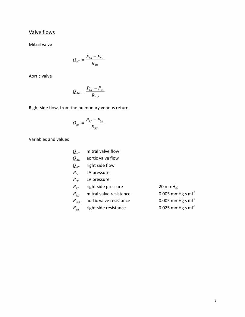
8

2

9

MI

LVLA

MIR

PPQ

−=

#

AO

SALV

AOR

PPQ

−=

, 2

RS

LARS

RSR

PPQ

−=

$

MIQ 2

AO

Q 2

RSQ 2

LAP "#

LV

P "

RSP 3'

MI

R 5' (

AO

R 5' (

RSR 35'

(

0

#

SA

ATSA

SAR

PPQ

−=

SA

SAVADAO

SAC

QQQP

−+=

#

AT

VSAT

ATR

PPQ

−=

AT

ATSA

ATC

QQP

−=

$

SA

Q 2

AO

Q 2

VAD

Q #72

AT

Q 2

SA

P

AT

P

VS

P '

SA

R 0' (

AT

R 15' (

SA

C 5'

(

AT

C '

(

Appendix B

Matlab Files

clear all

global Tc TLV delta phi

HR = 80; % heart rate in BPM, 80

Tc = 60/HR; % cardiac cycle period, SPB (sec per beat)

Tcp = 0.75; % sec, pump aspiration time per cycle

% "Rori" parameters for the orifice delta pressure i.e. dP = Rori * Q|Q|

% note, this is theoretical value, used only for base model simulations

Cd = 0.3; % friction factor, geometry of the orifice dependent

ro = 1060; % kg/m^3, density blood

d1 = 0.0558; % m, LV end diastolic diameter, person w/ 1.5 m^2 of skin area

d2 = 0.01854; % m, diameter cannula

Ac= (d2)^2*pi/4; % m^2, cannula orifice area

Rori=ro/2/(Cd/sqrt(1-(d2/d1)^4))^2/Ac^2;

% motor parameters

Km = 0.124; % (V sec)/rad, constant gyrator coefficient

Rm = 2.6; % Ohms, two phases in series resistance

Rb = 8.1e-5; % (N m sec)/rad, damping coefficient of motor

L = 2.58e-3; % H, inductance of two phases in series

56

Ip = 1.851e-5; % kg m^2, mass moment of inertia, piston

Ap = 2e-4; % m^2, area piston, 1cm x 2cm

r = 0.03; % m, moment arm to piston, assumed value %0.03

Vin = 11; % V, supply voltage, 0 - 14V

% inlet cannula

rho = 1060; % kg/m^3, density blood

Lc = 0.5; % m, cannula length

d2 = 0.01854; % m, diameter cannula

Ac = (d2)^2*pi/4; % m^2, cannula orifice area

Ic = rho*Lc/Ac; % kg/m^4, fluid inertia in the cannula

E = 500e6; % Pa, Young’s modulus PTFE material

v = 0.46; % no units, Poisson’s ratio for PTFE

tc = 0.002; % m, cannula wall thickness

Vc = pi*(d2/2)^2*Lc; % m^3, cannula volume

Cc = 2*Vc*(d2/2)*(1-v/2)/E/tc; % m^3/Pa, cannula compliance

% left ventricle

ELVmax = 2; % maximum LV elastance, mmHg/mL

ELVmax = ELVmax*1.333e8; % Pa/m^3

TLV = 0.44; % LV contraction time, s

delta = 0.6; % elastance peak percent shift

ALV = 0.01; % passive elastance coefficient, mmHg

ALV = ALV*133.3; % Pa

BLV = 0.06; % passive elastance coefficient, 1/mL

BLV = BLV*1e6; % 1/m^3

% left atrium

ELAmax = 0.05; % mmHg/mL

57

ELAmax = ELAmax*1.333e8; % Pa/m^3

TLA = 0.06; % LA contraction time, s

ALA = 0.44; % passive elastance coefficient, mmHg

ALA = ALA*133.3; % Pa

BLA = 0.049; % passive elastance coefficient, 1/mL

BLA = BLA*1e6; % 1/m^3

% arterial system

CSA = 5e-5; % systemic artery compliance, mL/mmHg

CSA = CSA*7.502e-9; % m^3/Pa

CAT = 1; % artery tree compliance, mL/mmHg

CAT = CAT*7.502e-9; % m^3/Pa

RSA = 0.04; % systemic artery resistance, mmHg s/mL

RSA = RSA*1.333e8; % Pa-s/m^3

RAT = 0.79; % artery tree resistance, mmHg s/mL

RAT = RAT*1.333e8; % Pa-s/m^3

% valve flows

RMI = 0.005; % mitral valve resistance, mmHg s/mL

RMI = RMI*1.333e8; % Pa-s/m^3

RAO = 0.005; % aortic valve resistance, mmHg s/mL

RAO = RAO*1.333e8; % Pa-s/m^3

RRS = 0.025; % right side resistance, mmHg s/mL

RRS = RRS*1.333e8; % Pa-s/m^3

% inputs

PRS = 20; % right side pressure, mmHg

PRS = PRS*133.3; % Pa

PVS = 10; % venous system pressure, mmHg

PVS = PVS*133.3; % Pa

% Initial conditions

VLVo = 4; % zero pressure volume, mL

VLVo = VLVo*1e-6; % m^3

VLAo = 5; % zero pressure volume, mL

VLAo = VLAo*1e-6; % m^3

VSAo = CSA*75*133.3;

58

VATo = CAT*75*133.3;

tend = 5*Tc; % sec, simulation length, 5 heart beats

%%%%%%%%%%%%%%%%%%%%%%%%%%%%% simulation command %%%%%%%%%%%%%%%%%%%%%%%%%%

sim(’pump_and_CVS_v3’)

%%%%%%%%%%%%%%%%%%%%%%%%%%%%%%%%%%%%%%%%%%%%%%%%%%%%%%%%%%%%%%%%%%%%%%%%%%%

figure(1)

subplot(3,1,1), plot(tout,PLV/133.3,tout,PLA/133.3,tout,PSA/133.3)

legend(’PLV’,’PLA’,’PSA’)

title(’Pressures, mmHg’)

axis([0 3.75 0 150])

subplot(3,1,2), plot(tout,simout_vlv*1e6,’red’,tout,PLV/133.3,’blue’)

title(’PLV (blue) mmHg and VLV (red) ml’);

axis([0 20 -100 100])

subplot(3,1,3), plot(tout,QAO*6e4,tout,simout_pumpflow*6e4)

title(’Aortic Valve Flow (blue) L\min, Pump Flow (green) L/min’)

axis([0 3.75 0 50])

figure(2)

% plot double y axis

[AX,H1,H2] = plotyy(tout,simout_cur,tout,simout_track);

xlabel(’t (sec)’)

set(get(AX(1),’Ylabel’),’String’,’Current (Amp)’)

set(get(AX(2),’Ylabel’),’String’,’Piston Position (Deg)’)

59

figure(3)

% plot PV loop

plot(simout_vlv*1e6,PLV/133.3)

xlabel(’V (mL)’), ylabel(’P (mmHg)’)

figure(4)

% plot resistance across the orifice vs. volume LV

plot(simout_vlv*1e6,simout_Rori)

xlabel(’V (mL)’), ylabel(’R__ori (Pa m^3/sec)’)

% save suction function R=R(Vlv)

% 3.26E10 + 4.56E10*exp(-28689.6*u)

60

ow

rate

into

VA

D

ow

rate

from

VA

DSi

mpl

e CV

S M

odel

v1. 1

0/13

/08

jg,rg

l

Q p

ump

to C

VS

PUM

P <<

<−−−

−−−−

−−−−

−−−−

−−−−

−−−−

−−−−

−−−−

−−−−

−−−−

−−−−

−−−−

−−−−

−−−−

−−−−

−−−−

−−−−

−−−−

−−−−

−−−−

−−−−

−−−−

−−−−

−−−−

>>>C

VS

doub

le c

lick

to c

hang

e

doub

le

clic

k to

cha

nge

****

****

***C

ontin

uous

Tra

ckin

g Cu

rve*

****

****

*

QA

O_

4PSA3

PLA

_2

PLV_1

sqrt

2

sqrt

sqrt

1

sqrt

sqrt

sqrt

m2c

m

100

i

1/L

1 s

gam

ma_

dot

Ic*A

p*r/

Ip

eLV,

eLA

eLV

f(u)

eLA

f(u)

delta

Vol

ume

com

plia

nt tu

be (m

^3)

dP_o

ri −

Pres

sure

Acr

oss

Ori

cecm

ps2l

pmin

2−K

−

cmps

2lpm

in1

−K−

cmps

2lpm

in

−K−

cm2m

l

−K−

Vr

Rm/L

Volu

me

LV (m

l)

Volta

ge

Vm

Km/Ip

View

Tra

ckin

g Cu

rve9

View

Tra

ckin

g Cu

rve8

View

Tra

ckin

g Cu

rve7

View

Tra

ckin

g Cu

rve5

View

Tra

ckin

g Cu

rve4

View

Tra

ckin

g Cu

rve3

View

Tra

ckin

g Cu

rve2

View

Tra

ckin

g Cu

rve1

1

View

Tra

ckin

g Cu

rve1

0

View

Tra

ckin

g Cu

rve1

View

Res

ultin

gSy

nchr

onou

s T

rack

ing

Curv

e (3

.75

sec

long

, i.e

. 10

pum

p st

roke

s)(3

60 d

eg p

er 0

.75/

2 se

c of

str

oke

leng

th)

VSA

dot

VSA1 s

VLVd

otVL

V1 s

VLA

dot

VLA1 s

VATd

otVA

T1 s

Tr

Rb/Ip Tp

Ap*

r

To W

orks

pace

9

sim

out_

Rori

To W

orks

pace

8

sim

out_

trac

k

To W

orks

pace

7

sim

out_

curf

To W

orks

pace

6

sim

out_

pum

pow

To W

orks

pace

5

sim

out_

vlv

To W

orks

pace

4

sim

out_

cur

To W

orks

pace

3

QA

O

To W

orks

pace

2

PSA

To W

orks

pace

14

sim

out_

pid

To W

orks

pace

13

sim

out_

pow

To W

orks

pace

12

sim

out_

pp

To W

orks

pace

11

sim

out_

diam

To W

orks

pace

10

sim

out_

der

To W

orks

pace

1

PLV

To W

orks

pace

PLA

Tm

Km

Tc1

Tc

TcTc

Sync

hron

ous

Trac

king

Cur

veG

ener

ator

9

f(u)

Sync

hron

ous

Trac

king

Cur

veG

ener

ator

8

f(u)

Sync

hron

ous

Trac

king

Cur

veG

ener

ator

7

f(u)

Sync

hron

ous

Trac

king

Cur

veG

ener

ator

5

f(u)

Sync

hron

ous

Trac

king

Cur

veG

ener

ator

4

f(u)

Sync

hron

ous

Trac

king

Cur

veG

ener

ator

3

f(u)

Sync

hron

ous

Trac

king

Cur

veG

ener

ator

2

f(u)

Sync

hron

ous

Trac

king

Cur

veG

ener

ator

11

f(u)

Sync

hron

ous

Trac

king

Cur

veG

ener

ator

10

f(u)

Sync

hron

ous

Trac

king

Cur

veG

ener

ator

1

f(u)

Suct

ion

Func

tion:

Base

d on

Exp

erim

anta

lD

ata

f(u)

Suct

ion

Even

t Cur

ve

Satu

ratio

n

Resu

lting

Sync

hron

ous

Tra

ckin

g Cu

rve

f(u)

Resi

stan

ceor

ice

nosu

ctio

n

Rori

QRSf(u

)

QM

I

f(u)

QA

O

f(u)

Q p

ump

Ap*

r/Ip

Pum

p Fl

oww

(L/m

in)

Prod

uct1

Prod

uct

Pres

sure

can

nula

(Pa)

Ppis

ton

(Pa)

Pow

er S

atur

ated

Posi

tion

Sens

or

Pist

on A

ngul

ar V

eloc

itySh

aft

Posi

tion

Volts

Pist

on P

ositi

onVo

lts/D

egre

es

Pc

1/Cc

PVS

PVSPR

S

PRS

PLV

f(u)

PLA

f(u)

Om

ega

1/Ip

Mat

hFu

nctio

n1

mod

Mat

hFu

nctio

n

mod

LV s

hort

axi

s di

amet

er (m

)

Inte

grat

or1

1 s

Inte

grat

or

1 s

Gro

und

GSA

−K−

GA

T

−K−

Flow

Qic

(L/m

in)

Filte

red

pum

p Fl

ow (L

/min

)

Fcn

f(u)

Der

ivat

ive

du/d

t

DPS

A

DPR

S

DPM

I

DPA

TD

PAO

Curr

ent U

nFilt

ered

(Am

ps)

Curr

ent F

ilter

ed (A

mps

)

Curr

ent D

eriv

ativ

e1

PID

Conn

ect/

Dis

conn

ect

the

Pum

p to

CVS

Conn

ect/

Dis

conn

ect

Suct

ion

Even

t

Conn

ect/

Dis

conn

ect

Satu

ratio

n Li

mit

Cloc

k2

Cloc

k

CSA

−K−

CAT

−K−

Aor

tic V

alve

Flo

w

Ang

ular

Vel

ocity

Filt

er7

1

0.05

s+1

Filt

er6

1

0.05

s+1

Filt

er5

1

0.05

s+1

Filt

er4

1

0.05

s+1

Filt

er3

1

0.05

s+1

Filt

er2

1

0.05

s+1

Filt

er1

1

0.05

s+1

Filt

er1

0.05

s+1

VLVd

ot

Vlv

Vlv

Vlv

PRS

VLA

dot

QRS

PLA

PLA

PLV

PLV

PLV

QM

I

QM

I

QM

I

VSA

dot

PSA

PSA

PSA

PSA

QA

O

QA

OQ

SAQ

SAQ

SAVA

Tdot

PAT

PAT

QA

TPV

S

h

h

h

h

h

h

h_do

t

h_do

t

Ppga

mm

a_do

t

Qp

Qp

Qp

lam

bda

lam

bda

Vin

Vt_d

otVt

Pt

Pt

Pt

dP_o

ri

Qic

Qic

Figure B.1: Pump and CVS Simulink Model

61

Bibliography

[1] M. Awasthi. Development of a cardio-vascular simulator for evaluation of ventricular

assist devices. Master’s thesis, University of Illinois at Urbana-Champaign, 2003.

[2] L. Baloa. Certainty-weighted system for the detection of suction in ventricular assist

devices. PhD thesis, University of Pittsburgh, Pittsburgh, PA, 2001.

[3] W. Borutzky. Bond Graph Methodology: Development and Analysis of Multidisci-

plinary Dynamic System Models. Springer-Verlag london Limited, Germany, 1st edi-

tion, 2010.

[4] P. Breedveld and J. van Amerongen. Dynamische systemen: modelvorming en simulatie

met bondgrafen. Technical report, Open Universiteit, Enschede.

[5] A. Brostrom. Information point. J Clin Nurs, 12(2):234–234, 2003.

[6] F. Cassot, D. Morvan, P. Issartier, and R. Pelissier. New versatile physical model

fitting the systemic circulation accurately. Medical and Biological Engineering and

Computing, 23:511–516, 1985.

[7] A. J. Clegg, D. A. Scott, E. Loveman, J. Colquitt, J. Hutchinson, P. Royle, and

J. Bryant. The clinical and cost-effectiveness of left ventricular assist devices for end-

stage heart failure: a systematic review and economic evaluation. Health Technol

Assess, 9(45):1–148, 2005.

[8] D. V. Cokkinos and B. S. Lewis. Heart failure overview. Heart Failure Reviews,

11(2):193–197, 2006.

[9] A. A. Elkamhawy and H. Chandna. Minimum detectable defect thickness in spect

myocardial perfusion test: Phantom study with 99mTc and 201Tl. J Nucl Med Technol,

29(4):183–188, 2001.

[10] K. Eya, E. Tuzun, J. Conger, H. K. Chee, D. Byler, C. Nojiri, O. H. Frazier, and

K. Kadipasaoglu. Effect of pump flow mode of novel left ventricular assist device

62

upon end organ perfusion in dogs with doxorubicin induced heart failure. ASAIO J,

51(1):41–49, 2005.

[11] J. D. Faires and R. L. Burden. Numerical Methods. Brooks Cole, 3rd edition, 2002.

[12] A. Ferreira, M. A. Simaan, J. R. Boston, and J. F. Antaki. Frequency and time-

frequency based indices for suction detection in rotary blood pumps. IEEE Xplore,

2:1064–1067, 2006.

[13] J. Freiberg. Absolute quantitation of left ventricular wall and cavity parameters using

ECG-gated PET. Journal of Nuclear Cardiology, 11(1):38–46, 2004.

[14] J. H. Gibbon. Application of a mechanical heart and lung apparatus to cardiac surgery.

Minn Med, 37(3):171–185, 1954.

[15] J. R. Gohean. A closed-loop multi-scale model of the cardiovascular system for eval-

uation of ventricular assist devices. Master’s thesis, Cockrell School of Engineering,

Univeristy of Texas at Austin, May 2007.

[16] S. Gregory, D. Timms, M. J. Pearcy, and G. Tansley. A naturally shaped silicone

ventricle evaluated in a mock circulation loop: A preliminary study. Journal of Medical

Engineering and Technology, 33(3):185–191, 2009.

[17] L. F. Hsu, P. Jas, P. Sanders, S. Garrigue, M. Hocini, F. Sacher, Y. Takahashi, M. Rot-

ter, J. L. Pasqui, C. Scave, P. Bordachar, J. Clmenty, and M. Hassaguerre. Catheter

ablation for atrial fibrillation in congestive heart failure. The New England Journal of

Medicine, 351(23):2373–2383, 2004.

[18] T. Korakianitis and Y. Shi. A concentrated parameter model for the human cardiovas-

cular system including heart valve dynamics and atrioventricular interaction. Medical

Engineering & Physics, 28(7):613–628, 2005.

[19] K. N. Litwak, S. Kihara, M. V. Kameneva, P. Litwak, A. Uryash, Z. Wu, and B. P.

Griffith. Effects of continuous flow left ventricular assist device support on skin tissue

microcirculation and aortic hemodynamics. ASAIO J, 49(1):103–107, 2003.

[20] K. N. Litwak, S. C. Koenig, R. C. Cheng, G. A. Giridharan, K. J. Gillars, and G. M.

Pantalos. Ascending aorta outflow graft location and pulsatile ventricular assist provide

optimal hemodynamic support in an adult mock circulation. Artif Organs, 29(8):629–

635, 2005.

63

[21] K. N. Litwak, S. C. Koenig, H. Tsukui, S. Kihara, Z. Wu, and G. M. Pantalos. Effects

of left ventricular assist device support and outflow graft location upon aortic blood

flow. ASAIO J, 50(5):432–437, 2004.

[22] J. D. Madigan, A. Barbone, A. F. Choudhri, D. L. Morales, B. Cai, M. C. Oz, and

D. Burkhoff. Time course of reverse remodeling of the left ventricle during support

with a left ventricular assist device. Journal of Thoracic and Cardiovascular Surgery,

121:902–908, 2001.

[23] D. G. Mason, A. K. Hilton, and R. F. Salamonsen. Reliable suction detection for

patients with rotary blood pumps. ASAIO Journal, 54:359–366, 2008.

[24] D. E. Mohrman and L. J. Heller. Cardiovascular Physiology (Lange Physiology Series).

McGraw-Hill, 5th edition, 2003.

[25] G. F. Morello. Method and system for detecting ventricular collapse. Patent, Feb 2007.

US 7175588.

[26] B. R. Munson, D. F. Young, and T. H. Okiishi. Fundamentals of Fluid Mechanics.

John Wiley & Sons, Inc., United States of America, 5th edition, 2006.

[27] G. M. Pantalos, S. C. Koenig, K. J. Gillars, G. A. Giridharan, and D. L. Ewert. Char-

acterization of an adult mock circulation for testing cardiac support devices. ASAIO

Jouranl, 50:37–46, 2004.

[28] Y. C. Pao, E. L. Ritman, R. A. Robb, and E. H. Wood. A finite element method for

evaluating cross-sectional Young’s Modulus of diastolic left ventricle. 1975. Proceedings

of 28th meeting of ACEMB, 385.

[29] K. Rasmusson, J. Hall, and D. Renlund. Heart failure epidemic boiling to the surface.

Nurse Pract, 31(11):12–21, 2006.

[30] W. J. Remme and K. Swedberg. Treatment of chronic heart failure. guidelines for the

diagnosis and treatment of chronic heart failure. Eue Heart J, 22(17):1527–1560, 2001.

[31] G. Rizzoni. Fundamentals of Electrical Engineering. McGraw-Hill, United States of

America, 1st edition, 2009.

[32] F. B. Sachse and G. Seemann. Modeling of cardiac electro-mechanics in a truncated

ellipsoid model of left ventricle. In Surgery Simulation and Soft Tissue Modeling, 2003.

Proceedings (Lecture Notes in Computer Science).

64

[33] D. Sobic-Saranovic, V. Bosnjakovic, S. Pavlovic, M. Veljovic, N. Kozarevic, J. Sapon-

jski, Z. Petrasinovic, M. Ostojic, V. Artiko, M. Todorovic-Tirnanic, and V. Obradovic.

Methods for the quantification of left ventricular volumes assessed by radionuclide

ventriculography (first part). Glas Srp Akad Nauka Med, NIL(48):11–30, 2005.

[34] P. Sundblad and B. Wranne. Influence of posture on left ventricular long- and short-axis

shortening. AJP - Heart and Circulatory Physiology, 283(1):1302–1306, 2002.

[35] P. U. Thamsen. Cutting clogging in wastewater systems. World Pumps., 2009.

This is an electronic document. Date of publication: March 25, 2009. Date re-

trieved: June 30, 2010. http://www.worldpumps.com/view/894/cutting-clogging-in-

wastewater-systems/.

[36] G. Tortora and S. Grabowski. Principles of Anatomy and Physiology. Harper & Row

New York, 1987.

[37] S. Vandenberghe, P. Segers, J. F. Antaki, B. Meyns, and P. R. Verdonck. Hemodynamic

modes of ventricular assist with a rotary blood pump: continuous, pulsatile, and failure.

ASAIO J, 51(6):711–718, 2005.

[38] S. Vandenberghe, P. Segers, B. Meyns, and P. Verdonck. Unloading effect of a rotary

blood pump assessed by mathematical modeling. Artif Organs, 27(12):1094–1101, 2003.

[39] O. Voigt, R. J. Benkowski, and G. F. Morello. Suction detection for the micromed

debakey left ventricular assist device. ASAIO Journal, pages 321–328, 2005.

[40] M. Vollkron, H. Shima, L. Huber, R. Benkowski, G. Morello, and G. Wieselthaler.

Development of a suction detection system for axial blood pumps. Artificial Organs,

28(8):709–716, 2004.

[41] A. L. Yettram and C. A. Vinson. Orthotropic elastic moduli for left ventricular me-

chanical behaviour. Medical and Biological Engineering and Computing, 17(1):25–30,

1979.

[42] W. Young and R. Budynas. Roark’s Formulas for Stress and Strain. McGraw-Hill

Professional, 7th edition, 2001.

[43] A. Yuhki, E. Hatoh, M. Nogava, M. Miura, Y. Shimazaki, and S. Takatani. Detection

of suction and regurgitation of the implantable centrifugal pump based on the motor

current waveform analysis and its application to optimization of pump flow. Artificial

Organs, 23(6):532–537, 1999.

65

[44] L. Zhong, D. N. Ghista, E. Y. Ng, and S. T. Lim. Passive and active ventricular

elastances of the left ventricle. BioMedical Engineering OnLine, pages 4–10, 2005.

[45] L. Zhong, D. N. Ghista, E. Y. Ng, S. T. Lim, R. S. Tan, and L. P. Chua. Explaining

left ventricular pressure dynamics in terms of LV passive and active elastances. J.

Engineering in Medicine, 220 Part H, 2006.

66

Vita

Djordje Adnadjevic was born in Belgrade, Serbia on 26 May 1985, the son of Nikola Adnad-

jevic and Darinka Adnadjevic. After obtaining his high school diploma at Warwick Valley

High School, NY, he received the Bachelor of Science degree in Electrical Engineering from

The University of Texas at Austin. He applied to The University of Texas at Austin for

enrollment in their mechanical engineering program. He was accepted and started graduate

studies in January, 2009.

Permanent Address: 910 Duncan Lane Apt 53

Austin, TX 78705

This thesis was typeset with LATEX 2ε∗ by the author.

∗LATEX 2ε is an extension of LATEX. LATEX is a collection of macros for TEX. TEX is a trademark of theAmerican Mathematical Society. The macros used in formatting this thesis were written by Dinesh Das,Department of Computer Sciences, The University of Texas at Austin, and extended by Bert Kay, James A.Bednar, and Ayman El-Khashab.

67