Embed Size (px)
Citation preview

Copyright
by
David Lee Clay
2017

The Thesis Committee for David Lee Clay
Certifies that this is the approved version of the following thesis:
RESERVOIR ANALYSIS AND
DEPOSITIONAL SYSTEMS OF THE UPPER
CRETACEOUS WOODBINE GROUP IN THE MEXIA FAULT
TREND OF THE EAST TEXAS BASIN:
MEXIA OIL FIELD
APPROVED BY
SUPERVISING COMMITTEE:
Richard Chuchla
William Ambrose
Eugene L. Ames, III
Thomas Ewing
Supervisor:
Co-Supervisor:

RESERVOIR ANALYSIS AND
DEPOSITIONAL SYSTEMS OF THE UPPER
CRETACEOUS WOODBINE GROUP IN THE MEXIA FAULT
TREND OF THE EAST TEXAS BASIN:
MEXIA OIL FIELD
by
David Lee Clay
Thesis
Presented to the Faculty of the Graduate School of
The University of Texas at Austin
in Partial Fulfillment
of the Requirements
for the Degree of
Master of Science in Energy and Earth Resources
The University of Texas at Austin
December 2017

Dedication
This thesis and the prior years of coursework are dedicated to my loving wife and our
daughter. They have given me the motivation and support to continue this journey of
completing my Master’s degree. The countless sacrifices that they have made to make this
possible deserve all the recognition in the world. They are given full credit for all of my
achievements. Without them my accomplishments would not be possible.
I would also like to dedicate this thesis to my parents for all of their years of sacrifice and
hard work to give me the opportunities that led me to this point in my life.

v
Acknowledgements
Gene Ames, III has been a mentor and advisor during the research and writing phases of
this thesis. He has provided his knowledge, expertise and his time. He also provided me with
confidence in choosing the thesis topic and encouraged me to focus on the historical and future
potential of the Woodbine Sandstones. Gene Ames also gave me the flexibility to advance my
academic career while growing my industry career. This flexibility in my early career has been
invaluable and greatly appreciated.
The honorable P. K. Reiter, of Mexia, is to be thanked for providing core data and countless
historical files. His father W. A. Reiter was the geologist who proposed the discovery well of
Mexia Oil Field. My thesis committee members have also been instrumental in guiding and
motivating my research and thesis. Bill Ambrose and Dr. William Fisher have provided numerous
guiding recommendations to advance research. All of their help and direction are greatly valued.
Richard Chuchla deserves special gratitude for encouraging me to not give up on finishing my
research. Without his motivation I likely would have allowed my thesis to go unwritten.
The University of Texas Energy and Earth Resources program, including Dr. Fisher and
Richard Chuchla, has provided an incredibly useful curriculum towards the pursuit of my degree.
My achievement of a unique degree like this is only made possible by all the faculty and staff of
the EER program. They are all very much appreciated.

vi
Abstract
RESERVOIR ANALYSIS AND
DEPOSITIONAL SYSTEMS OF THE UPPER
CRETACEOUS WOODBINE GROUP IN THE MEXIA FAULT TREND OF
THE EAST TEXAS BASIN:
MEXIA OIL FIELD
David Lee Clay, M.S.E.E.R.
The University of Texas at Austin, 2017
Supervisor: Richard Chuchla
Co-Supervisor: William Ambrose
The Mexia oil field, discovered in 1920, has produced 110 million barrels of oil from Upper
Cretaceous sandstone reservoirs of the Woodbine Group in Limestone County, Texas. The
producing Woodbine Group is primarily composed of siliciclastic sandstones, siltstones and
mudstones that have been divided by flooding surfaces into nine depositional cycles. Most of
these depositional cycles are fluvial-dominated deltaic in origin, with others of wave-modified
deltaic origin. The depositional cycles are important in defining reservoir heterogeneities in the
Mexia Fault Trend oil fields. The Woodbine sandstones are highly effective water-drive
reservoirs. However, historical field development methods, such as high-volume flow rates, were
ineffective at maximizing the fields’ recovery. This study is the first to recognize and map
individual Woodbine depositional cycles in the Mexia Fault Trend to explore how to maximize
future oil recovery efforts.

vii
This study also researched the historical development of the Mexia field cooperatively with
new digital production data sources. Combining historical production data with new mapping of
the depositional cycles and their net sandstones reservoir units uncovered significant bypassed oil
resources. Undrilled infill locations were identified, then analog production for each reservoir unit
was scaled to a field-wide redevelopment drilling program. In the Mexia field, this study indicates
an estimated 51 million barrels of oil remains to be produced. This analog study can be utilized to
assess other Mexia Fault Trend fields. The fault line fields contain approximately 559 million
barrels of original oil in place. A similar study on each individual oil field could lead to the
recovery of over 66 million additional barrels of oil.

viii
Table of Contents
List of Tables ........................................................................................................ xi
List of Figures ...................................................................................................... xii
Introduction: Woodbine Sandstone and Mexia Oil Field ..................................1
BACKGROUND .................................................................................................1
East Texas Basin ..................................................................................2
Mexia Field and Study Area Location ...............................................2
Woodbine Sandstone Reservoir ..........................................................3
OBJECTIVES ....................................................................................................4
Previous Work ........................................................................................................6
Mexia Field History and Production Characterization ......................................8
MEXIA FIELD DISCOVERY AND DEVELOPMENT ............................................8
MEXIA FIELD DRILLING EVOLUTION ..........................................................10
MEXIA FIELD PRODUCTION SUMMARY .......................................................12
OIL SOURCE AND GENERATION ...................................................................15
ORIGINAL OIL IN PLACE, RECOVERY FACTOR AND REMAINING OIL .......16
Methods .................................................................................................................19
NET SAND MAPPING .....................................................................................20
DEPOSITIONAL SYSTEM INTERPRETATIONS ................................................21
East Texas Basin Structural Setting ...................................................................23
REGIONAL BASIN SETTING ..........................................................................23
SALT RELATED STRUCTURES.......................................................................23
MEXIA FAULT TREND ..................................................................................24
MEXIA FAULT PLANE PROFILE ...................................................................27
Woodbine Group Stratigraphy ...........................................................................30
Woodbine Sandstone Net Sand and Facies Maps .............................................33
INTRODUCTION .............................................................................................34
S10 SEQUENCE BOUNDARY (SB_10) AND S10 FLOODING SURFACE
(MFS_10) .....................................................................................................37
S20 DEPOSITIONAL CYCLE ..........................................................................38
ix
S20 Wireline Log Curves...................................................................40
S20 Depositional System – Facies Interpretations ..........................40
S20 Reservoir Occurrences and Exploration Potential ..................42
S30 DEPOSITIONAL CYCLE ..........................................................................42
S30 Wireline Log Curves...................................................................44
S30 Depositional System – Facies Interpretations ..........................44
S40 DEPOSITIONAL CYCLE ..........................................................................45
S40 Wireline Log Curves...................................................................46
S40 Depositional System – Facies Interpretations ..........................48
S40 Reservoir Occurrences and Exploration Potential ..................49
S50 DEPOSITIONAL CYCLE ..........................................................................49
S50 Wireline Log Curves...................................................................51
S50 Depositional System – Facies Interpretations ..........................51
S50 Reservoir Occurrences and Exploration Potential ..................52
S60 DEPOSITIONAL CYCLE ..........................................................................53
S60 Wireline Log Curves...................................................................55
S60 Depositional System – Facies Interpretations ..........................55
S60 Reservoir Occurrences and Exploration Potential ..................56
S70 DEPOSITIONAL CYCLE ..........................................................................56
S70 Wireline Log Curves...................................................................57
S70 Core Description .........................................................................59
S70 Depositional System – Facies Interpretations ..........................61
S70 Reservoir Occurrences and Exploration Potential ..................62
S80 AND S90 DEPOSITIONAL CYCLES ..........................................................62
Future Mexia Field Development Potential .......................................................63
MEXIA FIELD PRODUCTION DECLINE AND ECONOMICS ............................63
DEVELOPMENT OF THE REMAINING OIL IN PLACE ....................................64
S20 Sandstone .....................................................................................65
S20 Economics ....................................................................................67
S50 Sandstone .....................................................................................69
S50 Economics ....................................................................................72
Lower S50 and S40 Sandstones ........................................................74

x
Lower S50 and S40 Economics .........................................................77
S70 Sandstone .....................................................................................78
S70 Economics ....................................................................................81
CUMULATIVE ECONOMICS OF FUTURE DEVELOPMENT .............................82
APPLICATION IN OTHER WOODBINE FIELDS ...............................................83
Conclusions ...........................................................................................................85
References .............................................................................................................87

xi
List of Tables
Table 1: Summary of Bureau of Mine’s Mexia field reservoir study
(Hill and Guthrie, 1943). .....................................................................................17
Table 2: Core plug analysis from whole core piece in the Hughey Oil
Company - Randall T White No. 1. ....................................................................59
Table 3: Economic inputs for S20, S50, Lower S50 and S70 wells. .................68
Table 4: Potential upside resources and economics for the S20 Reservoir. ...68
Table 5: Potential upside resources and economics for the S50 Reservoir. ...72
Table 6: Upside potential economics and resources for the Lower S50 and
S40 reservoirs. ......................................................................................................78
Table 7: Potential upside resources and economics for the S70 Reservoir. ...82
Table 8: Potential upside resources and economics for all Mexia
field reservoirs. .....................................................................................................83

xii
List of Figures
Figure 1: East Texas Basin Petroleum Province. Study area (in red) is located in the
Mexia-Talco Fault Trend. Modified from Ambrose and
others, 2009. .......................................................................................3
Figure 2: Historical drilling timeline for the Mexia field. The green bars illustrate the
number of wells drilling annually, whereas the blue line shows the
cumulative number of wells drilled. The Mexia field was heavily drilled
during the first five years of its history. A total of 806 well have been
drilled. ..............................................................................................10
Figure 3: Base Map of the Mexia field, include Texas Railroad Commission shapefile of
wells dating back to the 1920s without a digital file. Green attributes
indicate oil wells, pumping and shut-in. Blue attributes indicate disposal
wells. The trapping fault is traced in red and the green line is the lowest
known oil in the S50 reservoir unit. ..............................................12
Figure 4: Historical annual decline curve for the Mexia field. Green line illustrates
annual oil production. Early decline rate was approximately 30%, mid-life
decline was slightly less than 10% and late decline rate has been effectively
flat since 1998. .................................................................................13
Figure 5: Oil Sources for East Texas fields. Modified from Wescott, 1994. Mexia Fault
Trend Fields identified inside red box. .........................................15
Figure 6: Mexia Field structure map on the top of Main Pay Sand. Overlay of B.O.M.'s
lease categories. Lease block A is light blue, lease block B is purple, lease
block C is green and lease block D is dark blue. ..........................18
Figure 7: Triangular Classification of Deltaic Depositional Systems. From Galloway,
1975...................................................................................................21

xiii
Figure 8: Classification of Clastic Coastal Depositional Environments Schematic. From
Boyd, 1992. .......................................................................................22
Figure 9: Mexia fault graben schematic. Inter-graben faults are known to trap in the
Woodbine sands. The Megan Richey Field was discovered in 1987 and has
produced over 1.5 million barrels of oil. .......................................24
Figure 10: Structure map contoured on the MFS_90 (top of Woodbine). Faults were not
mapped into the structure; however, they are evident by the compressed
contours and rapid changes in elevation. Red traces are the basinward
normal faults in the graben system, whereas the blue traces are the
antithetic landward-dipping faults. Structural cross-section M-M’ is
illustrated by light blue line. ..........................................................25
Figure 11: Structural cross-section bisecting the Mexia Fault Graben structure. The
upthrown fault block to the east is the trapping structure where the Mexia
field is located. Inter-graben faults are present but not illustrated. Brown
lines indicate MFS_90, also known as the top of the Woodbine Formation
in this study. .....................................................................................26
Figure 12: Austin Chalk composite section with stratigraphic subdivisions from
Hovorka, 1998. The Austin Chalk section is located to the north of the
study area, in Ellis County, Texas.. ...............................................29
Figure 13: Mexia field fault plane profile. The outlined area in black is where
Woodbine is juxtaposed against Austin Chalk. The red outlined area is
where Woodbine is juxtaposed against Eagle Ford Shale. The spill point is
where Woodbine comes back into contact with Woodbine. The green
dotted line is the lowest known oil in the Mexia field. .................29
Figure 14: Depositional Systems Map of the Woodbine Formation. Study area in red
and Oliver’s interpreted depositional systems in green. Modified from
Oliver, 1971 and Dokur, 2012. .......................................................30

xiv
Figure 15a: (above) Stratigraphic column in the study area. The Mexia field is on the
Western shelf of the East Texas Basin. Modified from Ambrose et al., 2009.
...........................................................................................................32
Figure 15b: (right)Mexia Field Type Log. (API: 42-293-32392) Brown Oil and Gas Co.
– H.C. Roller No K2. MFS_10 through MFS_90 represents the entire
Woodbine Group in the study area. ..............................................32
Figure 16: Isopach (interval thickness) map of the undivided Woodbine Group. Section
contoured from above the MFS_10 to below the MFS_90. N-S Stratigraphic
Section marked in blue line. ...........................................................33
Figure 17: a) Woodbine Group Type Log from the southern study area - Mexia Field.
(API: 42-293-32392) Brown Oil and Gas Co. – H.C. Roller No K2. b)
Woodbine Formation Type Log from the northern study area. (API: 42-
394-34683) Medicine Bow Operating - Cheneyboro No. 1. .........35
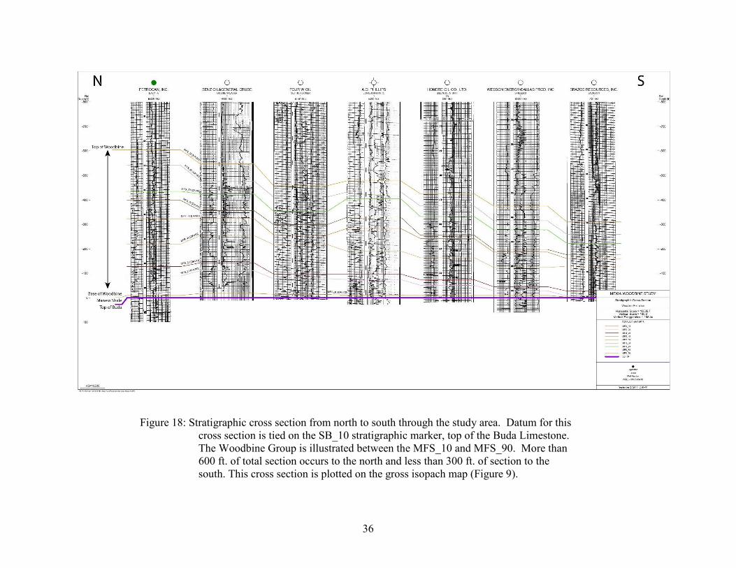
Figure 18: Stratigraphic cross section from north to south through the study area.
Datum for this cross section is tied on the SB_10 stratigraphic marker, top
of the Buda Limestone. The Woodbine Group is illustrated between the
MFS_10 and MFS_90. More than 600 ft. of total section occurs to the
north and less than 300 ft. of section to the south. This cross section is
plotted on the gross isopach map (Figure 9). ................................36
Figure 19: Paleogeographic reconstruction of the Upper Cretaceous in North America;
Late Albian/Early Cenomanian. Study area outlined in red box. (Modified
from Blakey, 2014). .........................................................................37
Figure 20: Lone Star Prod. - W. Anglin well log. This well is located in the southern
portion of the study area. ...............................................................37

xv
Figure 21: S20 net sandstone map. CI: 10 feet. The red box indicates the study area, the
red line indicates the Mexia field trapping fault and the green line indicates
the down-dip limit of the LKO (lowest known oil) in the Mexia field. SP
curves show wireline responses for different facies. The black arrowed lines
indicate the major depositional axes. ............................................39
Figure 22: Wireline SP curves from the S20 depositional cycle. Curves are posted on the
S20 net sandstone map. The logs are not to scale........................40
Figure 23: Boyd's classification of clastic coastal depositional environments schematic
with S20 depositional system interpretation (Boyd, 1992). .........41
Figure 24: S30 net sandstone map. CI: 10 feet. The red box indicates the study area, the
red line indicates the Mexia field trapping fault and the green line indicates
the LKO in the Mexia field. SP curves show wireline log response for
different facies. ................................................................................43
Figure 25: Wireline SP curves from the S30 depositional cycle. Curves are posted on the
S30 net sandstone map. The logs are not to scale........................44
Figure 26: Boyd's classification of clastic coastal depositional environments schematic
with S30 depositional system interpretation (Boyd, 1992). .........45
Figure 27: Wireline SP curves from the S40 depositional cycle. Curves are posted on the
S40 net sandstone map. The logs are not to scale........................46
Figure 28: S40 net sandstone map. CI: 10 feet. The red box indicates the study area, the
red line indicates the Mexia field trapping fault and the green line indicates
the LKO in the Mexia field. SP curves show wireline log response for
different facies. ................................................................................47
Figure 29: Boyd's classification of clastic coastal depositional environments schematic
with S40 depositional system interpretation (Boyd, 1992). .........48

xvi
Figure 30: S50 net sandstone map. CI: 10 feet. The red box indicates the study area, the
red line indicates the Mexia field trapping fault and the green line indicates
the LKO in the Mexia field. SP curves show wireline log response for
different facies. ................................................................................50
Figure 31: Wireline SP curves from the S50 depositional cycle. Curves are posted on the
S50 net sandstone map. The logs are not to scale........................51
Figure 32: Boyd's classification of clastic coastal depositional environments schematic
with S50 depositional system interpretation (Boyd, 1992). .........52
Figure 33: S60 net sandstone map. CI: 10 feet. The red box indicates the study area, the
red line indicates the Mexia field trapping fault and the green line indicates
the LKO in the Mexia field. SP curves show wireline log response for
different facies. ................................................................................54
Figure 34: Wireline SP curves from the S60 depositional cycle. Curves are posted on the
S60 net sandstone map. The logs are not to scale........................55
Figure 35: Boyd's classification of clastic coastal depositional environments schematic
with S60 depositional system interpretation (Boyd, 1992). .........56
Figure 36: Wireline SP curves from the S70 depositional cycle. Curves are posted on the
S70 net sandstone map. The logs are not to scale........................57
Figure 37: S70 net sandstone map. CI: 10 feet. The red box indicates the study area, the
red line indicates the Mexia field trapping fault and the green line indicates
the LKO in the Mexia field. SP curves show wireline log response for
different facies. ................................................................................58
Figure 38: Randall Oil Co. - T. White No. 1 well log. Cored interval 2,986 - 2,988 feet.
Core slab photos on right indicating facies changes in red and green lines.
...........................................................................................................60
Figure 39: Boyd's classification of clastic coastal depositional environments schematic
with S70 depositional system interpretation (Boyd, 1992). .........61

xvii
Figure 40: Mexia field monthly oil production and future decline. Provided by Corwin
Ames, Remora Petroleum, Austin, TX..........................................63
Figure 41: S20 Net sandstone map zoomed into the Mexia field. Average thickness on
the J. W. Reid lease is 15 feet. Purple polygon indicates potential S20 sand
productive reservoir; 2,307 acres. .................................................66
Figure 42: J.W. Reid lease cumulative daily production curve. 8 well lease commingled
together. ...........................................................................................67
Figure 43: S50 Net sandstone map zoomed into the Mexia field. Average net sand
thickness throughout the Mexia field is 45 feet. Purple polygon indicates
potential S50 sand productive reservoir; 3,432 acres. .................70
Figure 44: Hombre Oil Company - Billings Unit No. 1 S50 analog producer.71
Figure 45: Brown Oil Co. - H. C. Roller No. K2 log. Type log of the Upper and Lower
S50 Sands and the S40 Sands. ........................................................74
Figure 46: S40 Net sandstone map zoomed into the Mexia field. Average net sand
thickness throughout the Mexia field is 10 feet. Purple polygon indicates
potential Lower S50 and S40 sand productive
reservoir; 3,432 acres. .....................................................................75
Figure 47: Texas Alberta Oil - Barham No. 1 well log. Completed 6/23/1960. Perforated:
3,126-80'. ..........................................................................................76
Figure 48: Texas Alberta Oil - Barham No. 2 well log. Completed 10/11/1960.
Perforated: 3,078-79'. .....................................................................76
Figure 49: Production curve for the Barham No. 1 and No. 2 wells. Analog production
for the Lower S50 and S40 sandstones. .........................................77
Figure 50: S70 Net sandstone map zoomed into the Mexia field. Average net sand
thickness throughout the Mexia field is ~20 feet. Purple polygon indicates
potential S70 sand productive reservoir; 3,493 acres. .................79

xviii
Figure 51: Brown Oil and Gas Company - Freeman No. 1 monthly production curve.
...........................................................................................................80
Figure 52: Brown Oil and Gas Company - C. A. Kennedy No. 1 decline curve. Daily
production volume, S70 reservoir. ................................................81

1
Introduction: Woodbine Sandstone and Mexia Oil Field
The Upper Cretaceous siliciclasic Woodbine Group has long been an important economic
reservoir throughout the history of the oil industry. The Woodbine Group first became a producer
when oil was discovered in sandstone reservoirs in the Mexia field in Limestone County, Texas.
The Woodbine reservoirs are important to understanding how the State of Texas played such a
central role in the oil industry. For instance, the second largest oil field in the United States in
terms of original oil in place (OOIP), East Texas Oil Field, also produces primarily from the
Woodbine Group. The prolific nature of the wells in the Mexia field’s producing over 20,000
barrels of oil per day (BOPD) in the Woodbine Group encouraged northeastern oilmen to travel
south in the early 1920s and open up the East Texas Basin to exploration.
Since the discovery of the Mexia field, explorers have found over 11.6 billion barrels of
original oil in place in the Woodbine Group. The majority of these reserves were discovered prior
to the mid-1930s, before the Woodbine stratigraphy was thoroughly understood. The
heterogeneous nature of the interbedded sandstones and mudstones imparts complexity to these
reservoirs. Understanding these complexities requires detailed mapping of each depositional
cycle.
This study focuses on the Woodbine’s reservoir complexities. The Group was divided into
individual depositional cycles, which are separated by flooding surfaces. The cycles’ net sandstone
thickness was calculated and mapped. Net sandstone mapping was imperative to interpreting
depositional systems and how those systems control reservoir distribution in the Mexia Fault
Trend. These interpretations were then used to determine the best opportunities to produce
remaining oil reserves in the fault line fields.
BACKGROUND
In Limestone County, Texas, the Humphrey’s Oil Company completed the Rogers No. 1
in the Upper Cretaceous Woodbine Group in the fall of 1921 (Anonymous, 1947). This well, which
produced a modest 50 barrels of oil per day, opened the Mexia field and began the exploration and

2
development of the East Texas Basin. Mexia Oil Field is a mature field, which produced 110
million barrels of oil representing 99 percent of its 1983 estimated ultimate recovery (EUR),
suggesting that the field had reached is practical economic limit. However, advances in sequence
stratigraphy and today’s unconventional drilling and production techniques are important concepts
and tools for revitalizing mature fields. Understanding Woodbine reservoirs and how to best
develop secondary and tertiary reserves is important for future redevelopment efforts in the Mexia
field but also in other depleted giant reservoirs worldwide.
East Texas Basin
The East Texas Basin is a mature, heavily explored petroleum province. It is considered
to be a sub-basin to the Gulf of Mexico Basin forming during the initial opening of the Gulf of
Mexico during Jurassic time (Hammes et al., 2011). The basin is outlined by the Sabine Uplift on
the east, the Angelina-Caldwell Flexure to the south and the updip limits of Jurassic sediments to
the north and west (Figure 1). During the opening of the East Texas Basin, deposition and
subsequent withdrawal of the Louann Salt became the mechanism for structural deformation in the
basin, setting up petroleum traps associated with turtle structures, faults and salt-withdrawal
subbasins (Seni and Jackson, 1984). A line of normal faults often forming symmetrical grabens
occur along the updip limits of Jurassic salt; the basin continues landward to the north and west.
They were created by salt withdrawal during sediment accumulation. The formation of these
grabens, also known as the Mexia Fault Trend, is the structural element that creates the trapping
mechanism for the Woodbine Sandstone in the Mexia field.
Mexia Field and Study Area Location
The Mexia field and the study area are located on the western flank of the East Texas Basin
(Figure 1). The field is located in Limestone County, Texas and lies on the northwestern outskirts
of the town of Mexia for which the field was named. It was the first of multiple oil fields
discovered along the Mexia-Talco fault trend in East Texas. Wells in the field produced oil at very
impressive rates, some wells exceeding over 20,000 BOPD, but these high rates are thought to not

3
efficiently produce the Woodbine
reservoir. This likely resulted in oil
resources being left behind in the
reservoir. Surface mapping of
projected subsurface faults led to the
Mexia discovery and became the
exploration model for finding the
subsequent fields along the Mexia
Fault Trend. West and north of Mexia
the Woodbine sandstone was known to
be a source of freshwater and
suggested that the reservoir could be
prospective for oil exploration.
Woodbine Sandstone Reservoir
The Woodbine Group is
Cenomanian in age. It conformably
overlies the Buda Limestone and
underlies the Eagle Ford Shale (Hentz,
2014). The Woodbine Group occurs
throughout the East Texas Basin and continues south of the Cretaceous shelf edge, beyond the
Angelina-Caldwell Flexure in southeast Texas. In the study area, the Woodbine Group ranges in
thickness from over 900 ft. to the north and less than 300 ft. to the south. The predominant sand
source is from a northeastern deltaic system, which deposited siliciclastics from the northeast
towards the southwest into the basin center (Oliver, 1971 & Sohl, 1991). In the Mexia field area,
the Woodbine Group is known to be a high porosity reservoir that should be drained efficiently
during oil production and the study area is over 100 miles from the sediment source. In the past,
Figure 1: East Texas Basin Petroleum Province. Study
area (in red) is located in the Mexia-Talco
Fault Trend. Modified from Ambrose and
others, 2009.

4
net sandstone maps in the field area were never generated to the detailed of this study and the
stratigraphy was incompletely understood. This is one reason reservoirs at the Mexia field were
underdeveloped.
OBJECTIVES
The Woodbine Group and its multiple reservoirs are the focus of this study because they
are stratigraphically complex and have the potential for additional oil production. Defining the
stratigraphic elements of the Woodbine Group are important because few prior studies have been
conducted on the western margin of the East Texas Basin. The goal of interpreting depositional
environments of the Woodbine in the study area was achieved by producing net sandstone maps
of individual Woodbine depositional cycles. From the depositional cycles, mapping specific
reservoir bodies provided a framework for continued future secondary and tertiary development
in mature Woodbine fields along the Mexia-Talco fault trend. Historically, structural trapping
mechanisms were the primary focus of exploration of Woodbine reservoirs and hold significant
opportunity for future exploration. However, this study demonstrates how important the reservoirs’
stratigraphic complexities are to production and future development efforts.
The Mexia field was chosen specifically because its prolific production history is coupled
with an absence of efficient production practices. The field has produced over 100 million barrels
of oil from the Woodbine which is approximately 45% of the original oil in place (OOIP)
(Galloway et al., 1983). In most reservoir classes, 45% would be a high recovery factor but relative
to other Woodbine water-drive reservoirs this is not lackluster (Tyler et al., 1984). The reason is
likely that the field was discovered prior to proration and the resulting process of choking flow
rates back to more efficiently produce the oil in place (www.rrc.state.tx.us, 2017). Therefore, the
field was produced at peak rates during the early days of a true oil boom where the practice was
to: drill rapidly, produce rapidly to increase near term revenue and forestall oil theft. Large
volumes extracted at high flow rates likely caused inefficient oil drainage and preferential water
coning in these water-drive reservoirs. In particular, operators bypassed productive stringer sands

5
for high flow rates in the Mexia field’s “Main Pay” sand. Bypassing thin reservoirs was also
common later in the 1930s when East Texas Oil Field was being developed when operators drilled
through producing sands to producer higher flowing reservoirs (Ambrose et al, 2009). These
practices left significant oil reserves in place that will not be produced without targeted infill
drilling coupled with secondary or tertiary production efforts and possibly new drilling and
completion technologies. This study seeks to quantify the volume of oil left behind in the
Woodbine reservoirs in Mexia Oil Field and its attendant value. This work and the methods will
be helpful to other Woodbine reservoirs with similar production histories.

6
Previous Work
In the past, there were studies that covered the production of Woodbine reservoirs, such as
Hill and Guthrie, 1943 and studies that covered the structural and stratigraphic elements of the
Woodbine reservoirs, such as Oliver, 1971 but there were never studies that combined the two.
This study is fundamentally an independent review of the Woodbine Group in a local field area.
It is heavily influenced by previous stratigraphic and engineering studies of the Woodbine Group’s
sandstone reservoirs focused on the East Texas oil field. This study is influenced by the work of
Hentz, et al., published as Bureau of Economic Geology (BEG) Report of Investigation No. 274
that analyzed the sequence stratigraphy, depositional facies, petrography and reservoir attributes
of the Woodbine sands. Published in 2010, the study interpreted well log data, core data and
engineering production data. The report published four (4) individual topics in the report that
diligently reviewed the Woodbine reservoir sands throughout the East Texas oil field. The papers
were all beneficial in understanding where the value of this mature oil field can be found and how
to unlock that value.
Prior to the combined geological and engineering research efforts of the BEG, there were
broader, basin-wide studies published. In 1943, the United States Department of the Interior,
through the Bureau of Mines, published a Report of Investigations No. 3712 that analyzed the
production data of the Mexia Fault Trend oil fields (Hill and Guthrie, 1943). The study was purely
driven by production data and was published with the intent to summarize the historical production
of the prolific oil fields that produced from the Woodbine sands. There was very little attention
given to the stratigraphic or structural element of the reservoirs. The report summarized production
from the Mexia field, Wortham field, Currie Field, Richland Field and Powell Field.
Oliver (1971) interpreted the overall Woodbine Group sands using a net sand map of the
entire Woodbine Group and log facies, sorting the Woodbine Group sandstones in the context of
depositional systems. This study was purely a regional stratigraphic in scope, focused on
determining the principal depositional environments of the Woodbine Group. The study looked at

7
the entire basin and lumped all the Woodbine sands together and interpreted them as one deltaic
event. Oliver’s work was incorporated into this study which was more narrowly focused on the
Mexia field area.

8
Mexia Field History and Production Characterization
MEXIA FIELD DISCOVERY AND DEVELOPMENT
On November 19, 1920, the L. W. Rogers No. 1 well was brought in by Colonel E. A.
Humphreys at a depth of 3,065 to 3,117 feet. (Anonymous, 1947) One year before, the well was
spudded in September 1919 by John A. Sheppard from Oklahoma. The well was originally
proposed by an engineer and geologist team, Julius Fohs and W. A. Reiter, who believed that
surface faults extended down below the Woodbine Sands where the sands would be structurally
trapped. As these early oil industry stories typically unfold, Sheppard ran out of money before the
well could reach the total depth of the proposed 3,000 foot test well. Colonel Humphreys
purchased the well from Sheppard and continued drilling to the top of the Woodbine reservoir.
The well hit pay at 3,065 feet but the discovery only produced 50 BOPD however it proved that
oil was trapped in the Woodbine at depth. Col. Humphreys immediately began drilling 7 more test
wells. The second well came in at 200 BOPD, the third at 500 BOPD and within six months the
oil boom at Mexia was underway with the first gusher flowing at over 3,000 BOPD. The Rogers
No.1 and the Mexia field would forever change the history of the East Texas Basin. The Woodbine
reservoir was proved which would lead to the future discovery of other giant oil fields, including
East Texas Oil Field, a stratigraphic trap set up by the pinch out of Woodbine sand against the
Sabine Uplift. (Ambrose, 2009) It remains one of the largest stratigraphic traps ever found.
At the end of 1921, the Mexia field was producing from 64 wells at over 175,000 BOPD;
an average of about 2,735 BOPD per well and approximately 3,800 acres were proven productive
in the field. The field came online in a frenzy of activity with new fields being discovered along
strike to Mexia within the Mexia-Talco Fault Trend. In true oil boom fashion, people from all
around the nation flooded the area trying to capitalize on the discovery. In December of 1921
there were 67 wells producing and by December of 1922 there were 521 wells producing (Hill and
Guthrie, 1943). In 1922, those 521 wells produced approximately 34,000,000 barrels of oil, which
would be the peak year of production. In 1923, yearly production was reduced to approximately
18,000,000 barrels of oil, an indication that the dense and rapid drilling had prematurely drawn
9
down the oil reservoir. Per the U.S. Bureau of Mines, the Mexia field had produced approximately
73 percent of the ultimate recovery within 4.5 years (Hill and Guthrie, 1943).
In the early stages of field development, there were many deals to be done and fortunes to
be made. Col. Humphreys struck a historical deal for major oil companies to buy his crude from
the field. Hedging of future crude widely practiced in the industry in the 1920s but Humphreys
signed a contract which sold a one-third of his future crude at $1.50/barrel of oil. His proved oil
was set at 100,000,000 barrels of oil, so 33,333,333 1/3 barrels of oil were to be sold at
$1.50/barrel. Oil was trading at a higher price and Humphreys was selling at a discount, therefore
many were critical of his trade with the majors. However, in the early 1930’s when East Texas
Oil Field was discovered there was a flood of crude oil in the market, which caused a price collapse.
Oil went down to $0.10/barrel and Humphreys capitalized on his hedge. Eventually Col.
Humphreys sold out of his ownership. Pure Oil Company purchased the field in the mid-1920s
and continued production until the 1960s at which time they sold the field to a small independent
operator, Brown Oil and Gas Company. Since the change of operators, there has not been any
significant development. In fact, most wells in the field have been plugged with exception of
certain wells that are classified as stripper wells, or producing less than or equal to 10 BOPD.
Throughout the history of the field development there were no secondary recovery efforts.
It is believed that the early, rapid production led to wasted oil left in place without the proper
technology and methods to efficiently or economically produce remaining mobile oil. Field wide
production in recent years has roughly stayed flat and the field is thought to be prime for target
infill and secondary recovery efforts to improve the production rate.

10
MEXIA FIELD DRILLING EVOLUTION
After the Rogers discovery well, field development ramped up extremely fast with wells
brought onto production daily. The Rogers well was discovered in November 1920 and by year
end there was a total of two wells drilled. In 1921 there were 64 wells drilled and by 1922 there
were 351 more wells drilled, bringing the total wells to 417. This would be the peak of drilling
activity and peak production as well. After 1922 the production and drilling activity only declined.
By 1925, 85 percent of the total wells in the field were drilled. As seen by the historical drilling
chart, there were approximately 0 to 5 wells drilled per year going forward. These additional wells
did not replace declining production. However, during the later life of the field it did reduce the
decline rate, which resulted in incremental reserves growth (Figure 2).
Figure 2: Historical drilling timeline for the Mexia field. The green bars illustrate the
number of wells drilling annually, whereas the blue line shows the
cumulative number of wells drilled. The Mexia field was heavily drilled
during the first five years of its history. A total of 806 well have been
drilled.
11
Colonel Humphreys originally operated the majority of the Mexia field wells until he sold
his ownership to Pure Oil Company in 1923 (Anonymous, 1947), and by that time the field had
begun entering its declining stages. From 1924 to the 1960s when Pure Oil Company sold its
ownership, they had drilled a total of 47 wells. There is no evidence that they employed any type
of waterflood or pressure maintenance program. There were disposal wells, which replaced water
produced back into the Woodbine reservoir, but they were not utilized to as a patterned waterflood
program. Wells that were dry holes or depleted producers were simply converted to disposal wells
to capture some value. Pure Oil eventually sold their interest in Mexia and Powell Fields to a local
operator named Kilmarnock Oil Company (C. L. Brown). Kilmarnock later changed its name to
Brown Oil and Gas Company which operates the field currently. In the 1970s through 1987,
Brown Oil and Gas Company added approximately 25 producing wells, which gave the production
decline a noticeable bump, although decline continued soon after drilling ceased. In 2000, Brown
Oil and Gas Company began another drilling program and added 24 wells between 2000 and 2014.
During this time the decline was fully arrested and has remained flat since then. Brown Oil and
Gas took advantage of producing oil from a few sand stringer units that were not fully developed
during the early days of drilling. These sands still had oil remaining in place that was never
produced. This activity is the reason behind a flat production curve. However, if reserves are not
replaced then decline will soon continue and the field will cease to produce.
The Mexia field saw rapid initial development but very little drilling later in its producing
life (Figure 2). In the field’s 96-year history, the field and immediate surrounding area had 806
wells drilled to or deeper than the Woodbine reservoir. Of the 806 wells, 659 were classified as oil
wells at some point in their history with the remaining 147 wells being dry holes, junked and
abandoned or disposal wells. There remain only 52 oil producers as of December 2016.

12
MEXIA FIELD PRODUCTION SUMMARY
Figure 3: Base Map of the Mexia field, include Texas Railroad Commission shapefile of
wells dating back to the 1920s without a digital file. Green attributes indicate
oil wells, pumping and shut-in. Blue attributes indicate disposal wells. The
trapping fault is traced in red and the green line is the lowest known oil in the
S50 reservoir unit.
D
U

13
Currently the Mexia field has 70 active wells, of which 52 are pumping oil producers, 8
shut-in oil producers and 10 disposal wells (Figure 3). On average, the field produced 165 BOPD
in 2016 or 3.23 BOPD per well. According to well tests reported to the Texas Railroad Commission
(TRC), the 52 active wells are producing 4,518 barrels of water per day (BWPD). The water
produced is only a yearly reported number and is just an approximate number that is specific to a
certain day and does not reflect actual averages throughout the entire year. The TRC requires
disposal wells to report H-10s, which summarized annual water disposed of and can be averaged
into a daily number. The 10 active disposal wells disposed of an average of 6,868 BWPD in 2015
(2016 H-10s are not available yet). If this number is used for producing wells, then it averages out
to 132 BWPD per well. This calculates to approximately a 2.4% oil cut per well; some wells have
Figure 4: Historical annual decline curve for the Mexia field. Green line illustrates annual oil
production. Early decline rate was approximately 30%, mid-life decline was
slightly less than 10% and late decline rate has been effectively flat since 1998.

14
a higher or lower oil cut and this is only used as an average. It is assumed that any future
development will need to include plans to dispose or re-inject large volumes of produced water.
The early production history of the field was rapid-paced and visible in the decline curve
(Figure 4). The field had produced over 50 million barrels of oil by the second full year of
production. In the first 10 years of production the field’s annual decline rate was an average of
29%, with wells watering out rapidly. 100 million barrels was surpassed by year 1947 and has
leveled off since. Single digit annual declines (were common during these years. As of December
2016, the Mexia field has produced a cumulative 110,387,637 barrels of oil. Infrequent drilling in
the late 1990s and forward has effectively arrested the previous production decline. Since 1998,
the field production has been essentially flat.

15
OIL SOURCE AND GENERATION
The primary source rocks in the East Texas Basin are of Cretaceous and Jurassic age
(Wescott, 1994). The Upper Cretaceous Eagle Ford Formation is of major importance in the East
Texas Basin and is the source for many giant oil fields, including East Texas Oil Field. The
migration pathway for most of the Upper and Lower Cretaceous generated hydrocarbons was to
the east towards the Sabine Uplift (Figure 5). The Eagle Ford is immature in the East Texas Oil
Field. However, hydrocarbons have migrated into the Woodbine sand from the basin center and
from the south where maturity levels were higher. On the western edge of the basin, the Eagle
Ford and Lower Cretaceous source rocks are also immature and therefore do not serve as the source
for the Mexia field. The Mexia Fault line fields are inferred to be charged by Jurassic sourced oil
based on Wescott’s 1994 oil sampling in the East Texas Basin major fields (Figure 5). This would
assume significant vertical migrations from
Jurassic source rock up the fault zones to Upper
Cretaceous Woodbine sandstone reservoirs.
The Smackover Formation occurs at
approximately 8,500’ feet below sea level in the
downthrown block and the Woodbine Group
occurs at approximately 3,000’ at the Mexia
field. This would equate to 5,500’ or more of
vertical migration.
Wescott (1994) has two hypotheses for
why Jurassic oil occurs in Upper Cretaceous
reservoirs. The most plausible hypothesis for
the Mexia field is that Jurassic oil migrated via
the trapping fault into the Woodbine Group.
Wescott (1994) suggests that oil migrated
through the fault driven by overpressure. Once
Figure 5: Oil Sources for East Texas fields.
Modified from Wescott, 1994.
Mexia Fault Trend Fields
identified inside red box.

16
the hydrocarbons reach a permeable reservoir, they would migrate into the pressure sink, i.e. the
Woodbine sands. The Mexia Fault would then reclose until the Jurassic source rock would become
overpressured again. This process would repeat until the Woodbine reservoir sands fill to their
spill point.
ORIGINAL OIL IN PLACE, RECOVERY FACTOR AND REMAINING OIL
The United States Department of the Interior, through the Bureau of Mines, published a
Report of Investigations that analyzed the oil production in the Mexia Fault Trend (Hill and
Guthrie, 1943). The Report of Investigations number 3712 was published long after the Mexia
field had produced the majority of the cumulative oil (Hill and Guthrie, 1943). The study covered
the historical production on the field prior to digital archives and up through 1943. It is thought to
be the most detailed data source for production data of the Mexia field. The Bureau of Economic
Geology also published a brief analysis of the Mexia field, which covered the original oil in place
(OOIP) volume and the recovery factor. The remaining oil is a critical number when deciding the
future development of the field.
The Bureau of Mines Report of Investigation number 3712 analyzed the Mexia field
production data by dividing the field area into four lease blocks (Hill and Guthrie, 1943). In Figure
6, the east edge leases are labeled as A, the east edge leases in north Mexia are labeled as B, the
central and southern leases are labeled as C, and the fault line leases are labeled as D (Figure 6).
The reasoning behind the categorization is unknown. The study gathered production data for each
lease block and summarized the area (in acres), number of producing wells, estimated thickness of
the S50 (Main Pay) reservoir, reservoir volume and oil recovered to date. The summary is shown
in Table 1. The study was published in 1943 when the field was still producing. Therefore, the
cumulative production is not accurate. Combining this study and Texas Railroad Commission data
together, the Mexia field has produced 110,387,637 barrels of oil as of the end of 2016.

17
In 1983, the Bureau of Economic Geology published that the Mexia field’s estimated
ultimate recovery (EUR) would be 110 million barrels of oil (MMBO). The publication estimated
the original oil in place to be approximately 244 MMBO, therefore a recovery factor of 45 percent.
The OOIP value was likely only including the S50 or “Main Pay” sand. The study underestimated
the EUR likely because the recovery factor was too small. The field has surpassed their estimate
already and has a very slight decline rate. In a field such as Mexia the economic limit of the field
can continue for a very long time if the operating expenses are kept at a minimum.
Table 1: Summary of Bureau of Mine’s Mexia field reservoir study (Hill and Guthrie, 1943).
Group Name Proved Acres Productive Wells Well Spacing
Estimated
Reservoir
Thickness Reservoir Volume EUR EUR/Acre EUR/Acre-foot EUR/well
Group A East Edge Leases 1,540.6 144.0 10.7 24.2 37,282.52 10,000,000 6,491 268 69,444
Group B Northeast Edge Leases 437.5 98.0 4.5 25.5 11,156.25 3,146,748 7,193 282 32,110
Group C Mid-dip Leases 946.5 127.0 7.5 55.3 52,341.45 33,000,000 34,865 630 259,843
Group D Fault Leases 873.4 264.0 3.3 58.6 51,181.24 56,500,000 64,690 1,104 214,015
3,798.0 633 6.5 40.9 151,961.46 102,646,748.00 28,310 571 143,853

18
Figure 6: Mexia Field structure map on the top of Main Pay Sand. Overlay of
B.O.M.'s lease categories. Lease block A is light blue, lease block
B is purple, lease block C is green and lease block D is dark blue.

19
Methods
The study area was chosen for the significant potential for future oil and gas development.
The study area, approximately 350 square miles in extent, has had over 4,150 wells drilled
throughout its history. Unfortunately, many were drilled before wireline logging tools were
commonly used (about 1936). A total of 1,049 open-hole wireline well logs were available for
this research study. The well logs included Gamma Ray (GR) curves, Spontaneous Potential (SP),
Resistivity, Density and Neutron Porosity. All of the resultant wireline log curves were used to
some extent to compile and reorganize data to better understand the Woodbine Group. GR and SP
wireline curves were of most importance when calculating net sand amounts and creating net
sandstone maps and depositional facies maps.
The open-hole raster logs were imported into IHS PetraTM software where they were depth-
calibrated to help recognize and correlate formation tops and maximum flooding surfaces.
Sequence boundaries could not be reliably picked using open-hole wireline logs due to the absence
of confirmative core rock data. Marine flooding surfaces were the critical surfaces to be
recognized on logs and served as time equivalent boundaries that reliably defined depositional
cycles throughout the study area. Within each depositional cycles, net sandstone values were
calculated with PetraTM and net sandstone maps were contoured. The net sandstone contouring
was highly influenced by the GR and SP curves, which were traced in Petra and posted on the net
sand maps. Wireline well log curves, net sandstone maps and one small piece of whole core were
used to interpret depositional facies and annotate the depositional environments directly onto the
net sandstone maps. Depositional systems were interpreted using Galloway’s triangular
classification of deltaic depositional systems and Boyd’s classification of clastic coastal
depositional environments (Galloway, 1975 and Boyd, 1992).
There was one piece of whole core obtained for this study, which is only two and one-half
ft. in length. This core was taken from the Randall Oil Company (Hughey Oil) – T. White No. 1
(API: 42-349-30529), which is located in Richland Oil Field, north of the Mexia field. Mr. P.K.

20
Reiter, of Mexia, graciously donated his piece of rock core to this study. The core was sent to
Weatherford Laboratories for determination of porosity and relative permeability analysis.
Porosity and grain density analysis was undertaken at 2,987.9, 2,987.1, and 2,986.3 ft. The core
data, although only a few feet, was integrated into the net sandstone maps and depositional system
maps.
Mr. P.K. Reiter also provided full access to his files, which were filled with historical data
from the Mexia field. The historical data were combined with digital IHS well data, digital
DrillingInfo well data and digital Texas Railroad Commission well data. These sources were
merged in a master spreadsheet that charts the drilling history of the Mexia field. Merged
production data provided a full history of field production data. The Report of Investigations #
3712 published by the United States Bureau of Mines in 1943 was the primary data source for
early production history of the field (Hill and Guthrie, 1943). Then DrillingInfo’s data was added
to these datasets to create a 1920 to present day annual production file. It is the most thorough
production database that is known to date for the Mexia field.
NET SAND MAPPING
Calculations of the net sand values in each depositional cycle was the primary focus for
this study and the net sand could not be calculated without detailed correlation of the flooding
surfaces; the flooding surfaces are the backbone to the study. Prior to making calculations, the
open-hole logs were imported to IHS Petra and depth registered. The Petra well log analysis
function allows for direct integration of data from the log into the database where it can be mapped.
A vertical sand cutoff line was added to each raster image well log’s SP curve; this cutoff line was
chosen based on an average shale line. Once this cutoff line was chosen, it was used to hand-
calculate the sand facies where the SP curve deflection was to the left of the cutoff line. A base
and top of each sand member was picked based on where the SP curve crossed the cutoff line to
the left and where it crossed back over the cutoff line to the right, respectively. This was repeated
for each sand member within each depositional cycle. IHS Petra was used to sum all of the sand

21
values within the depositional cycle which were then posted on each net sand map where the values
were subsequently contoured.
DEPOSITIONAL SYSTEM INTERPRETATIONS
The net sand maps generated from the well log data were interpreted for each depositional
cycle to determine depositional facies and classification of depositional environments. Log curves
were posted on each net sand map to depict facies and where facies changed. The facies were
directly integrated into the depositional system classification interpretation. Every log was taken
into account however only specific logs were posted on the net sand maps in order to help interpret
the depositional environments. Each posted log curve was exported from Petra and manipulated
in Adobe Illustrator where the SP curve was traced.
The interpretations of the various Woodbine depositional cycles were made based on all
available data compiled in
IHS Petra. The net sand
maps and open-hole log
curves were directly tied to
prior academic
publications. The
interpretations of each
depositional cycle used
guidelines and
characteristics published by
Galloway’s 1975 ternary
diagram of deltaic
depositional systems
(Figure 7). Also, in a much
more detailed manner, the Figure 7: Triangular Classification of Deltaic Depositional
Systems. From Galloway, 1975.
22
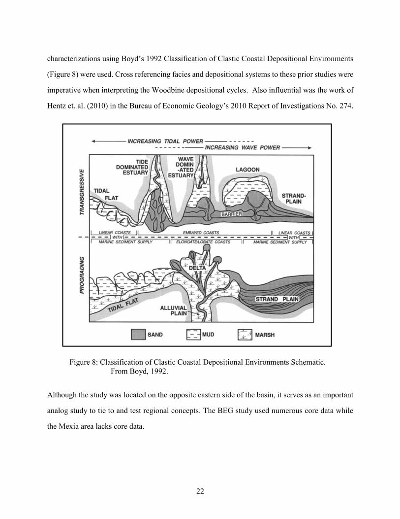
characterizations using Boyd’s 1992 Classification of Clastic Coastal Depositional Environments
(Figure 8) were used. Cross referencing facies and depositional systems to these prior studies were
imperative when interpreting the Woodbine depositional cycles. Also influential was the work of
Hentz et. al. (2010) in the Bureau of Economic Geology’s 2010 Report of Investigations No. 274.
Although the study was located on the opposite eastern side of the basin, it serves as an important
analog study to tie to and test regional concepts. The BEG study used numerous core data while
the Mexia area lacks core data.
Figure 8: Classification of Clastic Coastal Depositional Environments Schematic.
From Boyd, 1992.
23
East Texas Basin Structural Setting
REGIONAL BASIN SETTING
The first order controls on the geology of the basin were determined by pre-Jurassic
tectonics. The East Texas Basin is skirted by the Ouachita Thrust Front to the north and to the west
(Jackson, 1982). The basin is bounded to the south by the Caldwell-Angelina Flexure. On the
eastern border of the basin, the Sabine Uplift separates the North Louisiana Salt Basin. The East
Texas Basin formed simultaneously and began aggrading sediment with the opening of the Gulf
of Mexico Basin, which occurred during Early and Middle Jurassic time. The continued basin
subsidence allowed for a shallow sea and the Louann Salt evaporite was deposited basin-wide.
Mobilization of this early salt deposit under gravitational loading would become very important to
the petroleum resources of the East Texas Basin and most importantly the Mexia field, near the
western boundary of the basin. Many of the traps for major oil and gas fields in the basin are
predominately the result of salt tectonics. The updip limits of salt deposition lead to a rim of salt
withdrawal graben structures around the western and northern extents of the basin, which also
parallels the Ouachita Thrust Front (Seni and Jackson, 1984).
SALT RELATED STRUCTURES
The Louann Salt was deposited during the Middle Jurassic Period, when the basin was
forming and actively subsiding (Jackson, 1982). Salt deposits became mobile after deposition of
overlying strata in the Late Jurassic and Cretaceous Periods. Overburden pressure resulted in
basinward flow and evacuation of salt which created three different tectonic structural features.
Structures formed in fault bounded graben structures in the study area. As underlying salt was
evacuated basinward, younger sediments collapsed inward and downward. Secondary faulting
structures were salt pillows, compressed by moving salt and forced upward in an anticlinal
configuration. Pillow structures were accompanied by radial faulting. The third type of structures
caused by salt movement was salt diapers, compressed so much that they were eventually detached
from the mother salt and moved upward through denser strata. The salt domes were also associated

24
with radial faulting and were the most complex of salt-related structures. In the study area, the
first set of structures, fault-bounded grabens and extensional faults, form the dominant structural
styles.
MEXIA FAULT TREND
In the study
area, salt movement
caused graben
structures at the
headwall of the
down-to-the-basin
extensional system,
which set up the
Mexia field. As the
updip limit of salt
deposition was
parallel to the
Ouachita Thrust
Front, these fault
grabens develop a north-south strike, curving eastward near Hunt and Hopkins County and striking
east-west (Figure 1) (Jackson, 1982). The normal faults are very complex. They consist of a major
basinward-dipping normal fault detaching into salt and landward-dipping antithetic faults
bounding the graben structures (Figure 9). Many of the faults are difficult to trace with the quality
of available data. In the Powell and Mexia field areas, these splinter faults in the graben structures
serve to trap hydrocarbons in the Woodbine Group. The grabens tend to pinch out and form
discontinuous en echelon patterns (Figure 10). In the Mexia field, the major basinward fault forms
Figure 9: Mexia fault graben schematic. Inter-graben faults are known to
trap in the Woodbine sands. The Megan Richey Field was
discovered in 1987 and has produced over 1.5 million
barrels of oil.

25
the trapping
mechanism. The
juxtaposition across
the fault plane is
complex and
discussed further in
the next section. At
the top of the
Woodbine structure,
the fault throw on the
Mexia trapping fault
is >600 ft. This
trapping mechanism
is consistent in all of
the Woodbine fields
along strike in the
Mexia Fault Trend.
The trapping fault can
be mapped using
available open-hole
logs and it can also be
inferred from the
distribution of
original 1920s oil
wells and dry holes.
Figure 10: Structure map contoured on the MFS_90 (top of
Woodbine). Faults were not mapped into the structure;
however, they are evident by the compressed contours and
rapid changes in elevation. Red traces are the basinward
normal faults in the graben system, whereas the blue
traces are the antithetic landward-dipping faults.
Structural cross-section M-M’ is illustrated by light blue
line.
MEXIA
FIELD
M
M’
POWELL
FIELD
U
D
U
D
U
D
U
D
U
D

26
Figure 11: Structural cross-section bisecting the Mexia Fault Graben structure. The upthrown
fault block to the east is the trapping structure where the Mexia field is located.
Inter-graben faults are present but not illustrated. Brown lines indicate MFS_90,
also known as the top of the Woodbine Formation in this study.
M west
M’ east

27
MEXIA FAULT PLANE PROFILE
A fault plane profile was created to determine the structural controls on the Mexia fault
trap and seal. The Mexia fault has a maximum displacement of 660 feet (Figure 12). At the point
of maximum displacement, the Woodbine Group is juxtaposed against the Austin Chalk. The fault
displacement lessens along strike and the Woodbine is then juxtaposed against the Eagle Ford
Shale. The spill point is the location at which the upthrown Woodbine comes back into contact
with the downthrown Woodbine. The spill point controls the lowest known oil in the Mexia field
S50 reservoir. The field is a fault-dependent trap.
The juxtaposition of Woodbine against Eagle Ford Shale is an intuitively reasonable seal
because the Eagle Ford is known to be a fine-grained mudstone (Hentz et al., 2014). However,
the juxtaposition of the Woodbine against the Austin Chalk is more perplexing. The Austin Chalk
is a well recorded fractured reservoir in the East Texas Basin so there is reason to suspect that the
formation would leak. In the study area, the Lower Austin Chalk contains numerous marl and
bentonite intervals (Hovorka, 1998). It is likely that these ductile layers in the Chalk cause an
impermeable fault gouge in the zone of Woodbine/Austin Chalk juxtaposition to trap the oil
column in the Mexia field (Figure, 12).
The fault plane profile indicates that the fault is not symmetrical and that it grows in two
locations (central and to the northeast). This would infer that there are other compensating faults
in the northeast that were not mapped with the available data. The secondary fault and other
unmapped faults may serve to create traps and, therefore, offer upside potential in the Mexia field
area. Since the field is fault dependent, the oil would spill out from the trap and migrate updip and
further west to other potential fault traps. The opportunity exists for significant additional oil
resources in fault traps and understanding the structural complexities could be the key to unlocking
those resources.

28
Lower Chalk: Bentonite and Marl
Figure 12: Austin Chalk composite section with stratigraphic subdivisions
from Hovorka, 1998. The Austin Chalk section is located to the
north of the study area, in Ellis County, Texas.

29
Figure 13: Mexia field fault plane profile. The outlined area in black is where Woodbine is juxtaposed against Austin Chalk. The red
outlined area is where Woodbine is juxtaposed against Eagle Ford Shale. The spill point is where Woodbine comes back
into contact with Woodbine. The green dotted line is the lowest known oil in the Mexia field.
Woodbine/Chalk
gouge seal
Woodbine/Eagle Ford
LOWEST KNOWN OIL
Spill Point
Spill
660’
NE
SW

30
Woodbine Group Stratigraphy
The Woodbine Group is a combination of many sequences of siliciclastic mudstones,
siltstones and sandstones (Figure 15) (Ambrose et al., 2009). The Woodbine Group is Upper
Cretaceous (Cenomanian) and deposited between 100.5 – 93.4 mya (Hentz, 2010). The sediment
source for the Woodbine is the ancestral Ouachita Mountains in Oklahoma and Arkansas (Oliver,
1971). The silicilclastics were eroded from Paleozoic sedimentary and metamorphosed
sedimentary rocks and transported south and west then aggrading in the subsiding East Texas
Basin (Oliver, 1971). Woodbine
sediments entered the basin in the
northern portion of the basin and
prograded basin-ward towards the
south and southwest.
Oliver interpreted the
Woodbine deltaic event as three
systems, the Dexter Fluvial System the
Freestone Delta System and the shelf
strandplain system (Figure 14). The
Dexter Fluvial System is present in the
northern third of the East Texas Basin
whereas the Freestone Delta System is
further basin-ward. The Dexter
System is fluvial dominated and
greatly influenced by the tributary
systems, whereas the more distal
Freestone Delta System is a highly-
destructive deltaic system (Oliver,
Figure 14: Depositional Systems Map of the Woodbine
Formation. Study area in red and Oliver’s
interpreted depositional systems in green.
Modified from Oliver, 1971 and Dokur,
2012.

31
1971). Oliver interpreted the overall deltaic system by breaking it into depositional facies. The
study area is located within the Freestone Delta System and contains Oliver’s interpreted channel-
mouth bar facies, coastal barrier facies and prodelta-shelf facies (Figure 14). Hentz et al. (2010)
interpreted Oliver’s coastal barrier facies differently as a lowstand incised valley fill facies. The
study area does not include any valley fill facies.
A similar interpretation was made in the study area; however, the Woodbine Formation is
divided into nine depositional cycles, whereas Oliver interpreted the entire formation as one deltaic
cycle (Figure 15). The mapped flooding surfaces ranging from MFS_10 to MFS_90 are interpreted
as bounding depositional cycles within the Woodbine deltaic system. Each depositional cycle
consists of interbedded mudstones, siltstones and sandstones. MFS_10 is the flooding surface
boundary between the top of the Maness Shale and the lowest (oldest) Woodbine depositional
cycle. MFS_90 is the boundary between the top of the Woodbine Group (youngest) and the base
of the Eagle Ford Shale. In the study area, the Eagle Ford Shale is observed to be a siliciclastic,
organic-rich mudstone and is immature (Wescott, 1992). Prior to deposition of the Woodbine
Group, there was a major lowering of relative sea level after the Buda Limestone and Maness Shale
(Salvador, 1991; Mancini and Puckett, 2005).

32
Figure 15a: (above) Stratigraphic column
in the study area. The Mexia
field is on the Western shelf
of the East Texas Basin.
Modified from Ambrose et
al., 2009.
Figure 15b: (right) Mexia Field Type Log.
(API: 42-293-32392) Brown Oil
and Gas Co. – H.C. Roller No K2.
MFS_10 through MFS_90
represents the entire Woodbine
Group in the study area. S20
Fig
ure
14
(ab
ov
e):
Str
ati
gra
phi
S30
S30
S40
S40
S50
S50
S60
S60
S70
S70
S80
S80
S90
S90
S10
S10

33
Woodbine Sandstone Net Sand and Facies Maps
Figure 16: Isopach (interval thickness) map of the undivided Woodbine Group. Section contoured
from above the MFS_10 to below the MFS_90. N-S Stratigraphic Section marked in
blue line.
N
N
S
Figu

34
INTRODUCTION
In the northern portion of the study area the Woodbine Group is over 650 ft. thick and thins
to the south and southwest. In the southern part of the study area the Woodbine Group thins to
less than 300 feet. (Figure 16 and 17). The undivided Woodbine Group is defined as above the
MFS_10 marker, the top of Maness Shale, and below the MFS_90 or the base of the Eagle Ford
Formation (Figure 15). In this study, the Woodbine Group has been divided into depositional
cycles that are defined between flooding surfaces (Figure 15). The Buda Limestone was deposited
before the Woodbine depositional cycles began aggrading across the East Texas Basin. The top of
the Buda Formation is defined by sequence boundary 10. This represents a lowstand event,
followed by a transgressive interval between the SB_10 and the MFS_10, equivalent to the Maness
Shale. The MFS_10 marks the base of the Woodbine Group. The first depositional cycle of the
Woodbine, S20, is located above the MFS_10 and below the MFS_20. The cycle is an important
reservoir in the Mexia field, known locally as the Kollman Sand. The sand-poor S30 depositional
cycle is located between the MFS_20 and MFS_30. Depositional cycle S40 is located between
MFS_30 and MFS_40 and contains very little sand in the Mexia field area. Depositional Cycle
S50 is located between MFS_40 and MFS_50, this is locally known as the Main Pay sand and is
the major reservoir in the field. Depositional cycle S60 is located between MFS_50 and MFS_60;
there is no sand deposited in the field. Depositional cycle S70 is located between MFS_60 and
MFS_70 and serves as an important Mexia field reservoir. Similar to depositional cycle S20, this
is an important bypassed reservoir in the Mexia field known collectively as the Mexia Stringer
sands. Depositional cycle S80 is located between MFS_70 and MFS_80 and the depositional cycle
S90 is located between MFS_80 and MFS_90. These two depositional cycles contain little, to no
sandstone in the study area and do not serve as reservoirs but may serve as an effective seal for
underlying reservoir sands. To the north, closer to the sediment source, the S80 and S90
depositional cycles contain significant quantities of sand.

35
Figure 17: a) Woodbine Group Type Log from the southern study area - Mexia Field. (API:
42-293-32392) Brown Oil and Gas Co. – H.C. Roller No K2. b) Woodbine
Formation Type Log from the northern study area. (API: 42-394-34683)
Medicine Bow Operating - Cheneyboro No. 1.
Resistivity
GR and SP
Resistivity
GR and SP
MAIN
PAY
36
Figure 18: Stratigraphic cross section from north to south through the study area. Datum for this
cross section is tied on the SB_10 stratigraphic marker, top of the Buda Limestone.
The Woodbine Group is illustrated between the MFS_10 and MFS_90. More than
600 ft. of total section occurs to the north and less than 300 ft. of section to the
south. This cross section is plotted on the gross isopach map (Figure 9).

37
S10 SEQUENCE BOUNDARY (SB_10) AND S10 FLOODING SURFACE (MFS_10)
The stratigraphic units below the Woodbine Group are the Buda Limestone and Maness
Shale. The Buda Limestone is Upper Cretaceous (Lower Cenomanian) in age and was deposited
in an open-water shallow marine environment (Figure 19) (Blakey, 2014). The Buda Limestone
is consistent across the study area and typically 90 to 100 feet thick (Figure 20). However, few
wells penetrated the Buda Limestone
in the Mexia field because the main
target was the Woodbine Group.
There are no reports of any Buda
Limestone production other than a
few oil shows. Woodbine sandstones
aggrade onto the SB_10 and
MFS_10, which is the Buda
Limestone and the Maness Shale
section.
Figure 19: Paleogeographic reconstruction of the Upper Cretaceous in North
America; Late Albian/Early Cenomanian. Study area outlined in
red box. (Modified from Blakey, 2014).
Figure 20: Lone Star Prod. - W. Anglin well log. This well
is located in the southern portion of the study
area.
Base of Buda
Limestone
SB 10: Top of
Buda Limestone
MFS 10: Top of
Maness Shale

38
S20 DEPOSITIONAL CYCLE
The S20 depositional cycle occurs between the MFS_10 and MFS_20 (Figure 15). The
cycle is the oldest sandstone-bearing stratigraphic unit in the Woodbine. Sandstone deposition
occurs in the northern one-third of the study area, where it ranges from 0 to 80 ft. in thickness
(Figure 21). The net sandstone map indicates a possible sediment source from the northeast,
consistent with Oliver’s 1971 interpretation that infers a Woodbine source from the north and
northeast fringe of the East Texas Basin. The depositional axes follow dip-elongate sandstone
bodies and trend southwestward. Net sandstone thins out between the depositional axes. The
depositional axes further south (basinward) pinch out away from the northeastern source.
Depositional axes range from 5 to over 15 miles long and from 1 to 2.5 miles wide in the northern
end of the study area. Thickest sandstone bodies exhibit bifurcating patterns basinward, splitting
into 6 separate axes.

39
Figure 21: S20 net sandstone map. CI: 10 feet. The red box indicates the study area, the
red line indicates the Mexia field trapping fault and the green line
indicates the down-dip limit of the LKO (lowest known oil) in the Mexia
field. SP curves show wireline responses for different facies. The black
arrowed lines indicate the major depositional axes.

40
S20 Wireline Log Curves
Wireline log patterns can be indicative of depositional facies and overall depositional
environments when interpreted together with other wireline logs (Fisher et al., 1969). Wireline log
curve (1) in the northeast is upward-coarsening to a thick sandstone with a sharp, blocky top
(Figure 22). Wireline log (2) is similar, but without an upward-coarsening base. The wireline
response is blocky with a sharp top and base. The nature of these northeastern logs are consistent
with the net sandstone maps inferring thicker sand bodies in the northern study area whereas
sandstones to the south and west have wireline log responses that are serrate. Wireline log (3) is
upward-coarsening into a spiky, serrate response. Wireline log curve (4) contains multiple non-
uniform serrate responses. These southwestern wireline log patterns are consistent with more
distal, thin sandstone beds interbedded with mudstones with limited vertical connectivity.
S20 Depositional System – Facies Interpretations
There is no core information available for the S20 depositional cycle. Therefore,
interpretations were made using the net sandstone map and wireline log curves. The S20
depositional cycle is interpreted to be in a fluvial-dominated delta (Figure 23). It was moderately
influenced by wave reworking. The delta prograded from the northeast to the southwest. The
proximal depositional environment is indicated by an upward-coarsening distributary channel
system that fed from the delta front to the prodelta. The distributary axes are mostly straight but
Landward
2
3
4
Basinward
Figure 22: Wireline SP curves from the S20 depositional cycle. Curves are posted on the S20
net sandstone map. The logs are not to scale.
1

41
towards their terminations they deflect to the south, inferring slight wave reworking. The zero sand
line follows the western edges of the study area and then wraps around toward the south and east.
This elongate nature of the sand body indicates the sand was reworked by wave action to the south
and east. Delta front facies are interpreted in wireline log curves number 1 and 2, and prodelta
facies are interpreted by wireline log curves number 3 and 4. In the far southern part of the study
area sandstone is absent and the S20 depositional cycle is interpreted to be entirely composed of
mudstone in a distal, more basinal offshore environment.
Figure 23: Boyd's classification of clastic coastal depositional environments
schematic with S20 depositional system interpretation (Boyd, 1992).
S20 Depositional
System

42
S20 Reservoir Occurrences and Exploration Potential
The S20 sandstone is an important reservoir in the Mexia field. Net sandstone ranges from
30 feet thick in the northern edge of the field and pinches out to zero on the south edge of the field.
The sand was not discovered until a few months after the field came online (Anonymous, 1947).
The sandstone was named after the Kollman lease. The Kollman Sand, was not as productive as
the “Main Pay” Sand and was, therefore, not penetrated in many wells in the field. The S20
reservoir contains undeveloped resources that show potential for redevelopment since the reservoir
was not a primary target, during field development. The S20 is trapped along the same fault that
the S50 (“Main Pay”) is trapped against and suggests a large area for redevelopment. Having a
more detailed understanding of the depositional system in the S20 cycle will be important if these
potential resources are to be developed in the future.
S30 DEPOSITIONAL CYCLE
The thin S30 depositional cycle includes some sandstone in the majority of the study area.
The thickest sandstone (>15 ft.) was deposited in the northern part of the study area (Figure 24).
There is no S30 sandstone deposited south of the study area. The net sandstone map indicates a
minor depositional axis or a thicker sand body that is located in the north central part of the study
area. The depositional axis trend is from north-northeast to south-southwest. The sandstone bodies
are primarily straight and dip-elongate and thin toward the southern part of the study area. The S30
deposition greater than 0-5 ft. of sand is lobate but the thicker sand bodies are dip-elongate. The
system is up to 15 miles wide and the length of the system is greater than 30 miles long.

43
Figure 24: S30 net sandstone map. CI: 10 feet. The red box indicates the study area,
the red line indicates the Mexia field trapping fault and the green line
indicates the LKO in the Mexia field. SP curves show wireline log
response for different facies.

44
S30 Wireline Log Curves
Wireline log curves of the S30 sandstone, generally, are serrate and non-uniform (Figure
25). The wireline log curves for the S30 sandstone are mostly sharp and spiky. Throughout the
study area the S30 sandstone serves as a recognizable marker bed because its wireline log response
does not vary greatly.
S30 Depositional System – Facies Interpretations
The S30 depositional cycle is fluvial-dominated deltaic in origin with no evidence of wave
reworking, based on the dip-elongate, digitate net-sandstone geometry (Figure 24). The study area
is interpreted to be located within the distal prodelta region of the deltaic system. The S30
sandstone is, generally, non-uniform but consistent across the study area and is indicative of a
broad prodelta facies. Thin, serrate wireline log responses, down-dip bifurcating channels and
southwestward sandstone pinchout confirm this interpretation.
The S30 sandstone is not a known reservoir in the study area. There is no evidence of
attempted production from the reservoir. The sandstone has consistent low porosity and
permeability throughout the study area. The sand exhibits less than 10% porosity from wireline
density porosity curve in figure 15. It is reasonable to infer that the low porosity and permeability
have inhibited the S30 sandstone from being a productive conventional reservoir.
Landward
2
3
4
Basinward
Figure 25: Wireline SP curves from the S30 depositional cycle. Curves are posted on the S30
net sandstone map. The logs are not to scale.
1

45
S40 DEPOSITIONAL CYCLE
The S40 depositional cycle is characterized by sandstone over approximately 80 percent of
the study area, with net sandstone thickness exceeding 100 ft. in the north. A single dip-elongate
depositional axis enters the study area from the north and intersects multiple strike-elongate
depositional axes. The dip-elongate axis extends basinward, gradually pinching out in the
southwestern part of the study area (Figure 28). The dip-elongate axis is sinuous and is
approximately 5 miles wide and greater than 20 miles long. The strike-elongate sandstone bodies
are collectively straight and are approximately 10 miles wide. Individual sandstone bodies are less
than 1 mile wide. The length of the east-west bundle of sandstone bodies exceed 15 miles, but
Figure 26: Boyd's classification of clastic coastal depositional environments
schematic with S30 depositional system interpretation (Boyd, 1992).
S30 Depositional
System
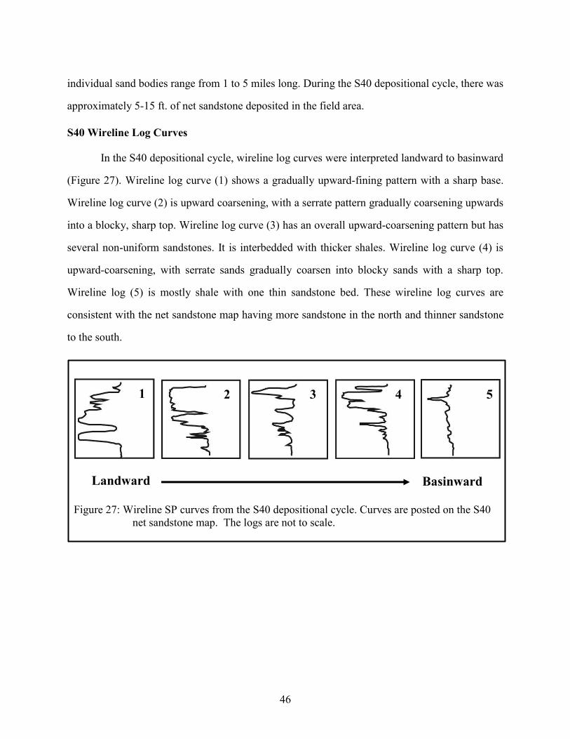
46
individual sand bodies range from 1 to 5 miles long. During the S40 depositional cycle, there was
approximately 5-15 ft. of net sandstone deposited in the field area.
S40 Wireline Log Curves
In the S40 depositional cycle, wireline log curves were interpreted landward to basinward
(Figure 27). Wireline log curve (1) shows a gradually upward-fining pattern with a sharp base.
Wireline log curve (2) is upward coarsening, with a serrate pattern gradually coarsening upwards
into a blocky, sharp top. Wireline log curve (3) has an overall upward-coarsening pattern but has
several non-uniform sandstones. It is interbedded with thicker shales. Wireline log curve (4) is
upward-coarsening, with serrate sands gradually coarsen into blocky sands with a sharp top.
Wireline log (5) is mostly shale with one thin sandstone bed. These wireline log curves are
consistent with the net sandstone map having more sandstone in the north and thinner sandstone
to the south.
3
1
4
Landward
Basinward
2
Figure 27: Wireline SP curves from the S40 depositional cycle. Curves are posted on the S40
net sandstone map. The logs are not to scale.
5

47
Figure 28: S40 net sandstone map. CI: 10 feet. The red box indicates the study area,
the red line indicates the Mexia field trapping fault and the green line
indicates the LKO in the Mexia field. SP curves show wireline log
response for different facies.
1
2
3
4
5

48
S40 Depositional System – Facies Interpretations
The S40 depositional cycle is interpreted to contain wave-dominated deltaic deposits with
moderate fluvial influence (Figure 29). The predominant sandstone bodies are strike-elongate
(east-west) and parallel and together delineate the paleoshoreline (Figure 28). Wireline log curve
(2) is interpreted as prograding shoreface facies. The lower, serrate sands grade into blockier,
thicker and coarser sandstones commonly associated with the transition from lower to upper
shoreface. The south-trending sandstone landward (north) of the shoreface is interpreted to be the
primary sediment distributary channel facies. The upward-fining wireline log curve (1) is
consistent with distributary channel deposit. Basinward of the shoreface, sediment is deposited
and reworked by wave action. Wireline log curve (4) is in the wave-modified delta part of the
depositional system. The prograding delta facies is being deflected by wave-action to the south
and west. Prodelta facies occur in the southern part of the study area and then grade into a muddy
offshore basinal environment.
Figure 29: Boyd's classification of clastic coastal depositional environments
schematic with S40 depositional system interpretation (Boyd, 1992).
S40 Depositional
System
49
S40 Reservoir Occurrences and Exploration Potential
The S40 depositional cycle is not a prominent reservoir in the Mexia field. In the Mexia
field area, the S40 facies is located in the prodelta facies. There is evidence of one well producing
from the S40 reservoir, which was commingled with another well producing from the lower S50
sandstones. The two wells together produced over 233,000 barrels of oil. The S40 sandstones
contain oil but have been overlooked because they are thin and discontinuous. Given the thin but
productive nature of the S40 sandstones, it could potentially serve as a future target.
S50 DEPOSITIONAL CYCLE
The S50 depositional cycle deposited sandstone over the entire study area (Figure 30). Net
sandstone in the S50 depositional cycle reaches a maximum of 70 ft. in the central part of the study
area goes to zero in the south. The net sandstone bodies are dip-elongate trending in sinuous
patterns in the northern and central part of the study area. The depositional axes bifurcate
basinward. The depositional axes are 1-2 miles wide and are greater than 20 miles long. In the
northeastern part of the study area the dip-elongate depositional axes are interrupted by
discontinuous, perpendicular sand bodies that are lobate and trend east-west. In the southern one-
third of the study area a bundle of sandstone bodies are strike elongate. There are multiple
sandstone bodies that are less than 2 miles wide, 1 to 5 miles long, and discontinuous. The southern
sandstone bodies, together, exhibit a lobate geometry.

50
Figure 30: S50 net sandstone map. CI: 10 feet. The red box indicates the study area, the
red line indicates the Mexia field trapping fault and the green line indicates
the LKO in the Mexia field. SP curves show wireline log response for
different facies.
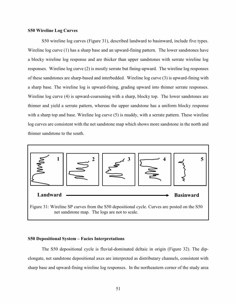
51
S50 Wireline Log Curves
S50 wireline log curves (Figure 31), described landward to basinward, include five types.
Wireline log curve (1) has a sharp base and an upward-fining pattern. The lower sandstones have
a blocky wireline log response and are thicker than upper sandstones with serrate wireline log
responses. Wireline log curve (2) is mostly serrate but fining-upward. The wireline log responses
of these sandstones are sharp-based and interbedded. Wireline log curve (3) is upward-fining with
a sharp base. The wireline log is upward-fining, grading upward into thinner serrate responses.
Wireline log curve (4) is upward-coarsening with a sharp, blocky top. The lower sandstones are
thinner and yield a serrate pattern, whereas the upper sandstone has a uniform blocky response
with a sharp top and base. Wireline log curve (5) is muddy, with a serrate pattern. These wireline
log curves are consistent with the net sandstone map which shows more sandstone in the north and
thinner sandstone to the south.
S50 Depositional System – Facies Interpretations
The S50 depositional cycle is fluvial-dominated deltaic in origin (Figure 32). The dip-
elongate, net sandstone depositional axes are interpreted as distributary channels, consistent with
sharp base and upward-fining wireline log responses. In the northeastern corner of the study area
3
1
4
Landward
Basinward
2
Figure 31: Wireline SP curves from the S50 depositional cycle. Curves are posted on the S50
net sandstone map. The logs are not to scale.
5

52
a channel levee splay is present, based on its serrate wireline log responses. The net sandstone
geometry is lobate and strike oriented. In the southern one-third of the study area the dip-elongate
(south-trending) distributary channels transition to strike-elongate (east-west-trending) patterns
that represents channel mouth bars reworked by wave action. The upward-coarsening pattern of
wireline log curve (4) indicates the channel mouth bar is upward-shoaling. Basinward from the
channel mouth bar, there are offshore sandbars reworked in a strike-elongate direction by wave
action. The sandstone then grades into offshore muddy facies further basinward.
S50 Reservoir Occurrences and Exploration Potential
The S50 depositional cycle, also known as the “main pay” sand, deposited sandstones that
serve as the primary reservoir unit in the Mexia field (Figure 30). The reservoir is interpreted as a
channel mouth bar and offshore sand bars. The S50 sandstone has produced over 110 million
Figure 32: Boyd's classification of clastic coastal depositional environments
schematic with S50 depositional system interpretation (Boyd, 1992).
S50 Depositional
System

53
barrels of oil, with some reserves contribution from S20 and S70 reservoir sandstones. The upper
sandstone unit with blocky wireline log responses (4) in the S50 is the main contributor to
production. However the lower, thinner sandstones contained significant reserves, based on the
Barham Lease wells completed in the 1960s, which is discussed in a later section. The upper S50
sandstone is mostly depleted but the lower sandstones have very significant potential because
many wells did not isolate and produced the lower sandstones. Isolating the lower sandstones
from the upper sandstones will be the crucial element to producing the remaining resources.
S60 DEPOSITIONAL CYCLE
The S60 depositional cycle contains sandstone in the northern one-half of the study area.
The net sandstone thickness reaches 60 ft. thick within the north-south depositional axes and
abruptly pinches out in the central part of the study area (Figure 33). The thick sand bodies are
dip-elongate and exhibit a sinuous pattern. They bifurcate southward and are less than one mile
wide and over 10 miles long. The depositional axes are narrow and thin to less than 20 ft. along
strike over a distance of less than 2 miles. In the central part of the study area, the dip-elongate
depositional axes pinch out north of the Mexia field.

54
Figure 33: S60 net sandstone map. CI: 10 feet. The red box indicates the study area, the
red line indicates the Mexia field trapping fault and the green line indicates
the LKO in the Mexia field. SP curves show wireline log response for
different facies.

55
S60 Wireline Log Curves
The S60 wireline log curves display log curve from north to south (Figure 34). Wireline
log curve (1) is upward-fining with a sharp base. The curve is mostly made up of one sand unit
and few mudstone interbeds. Wireline log curve (2) is less obviously upward-fining with a
relatively thicker upper sandstone bed. The curve has a sharp base and one shale break. Wireline
log curve (3) is mostly blocky with no overall pattern. The sandstone beds are non-uniform in
thickness, but all are blocky with sharp tops and bases. Wireline log curve (4) is a serrate pattern
with one sharp, sandstone. The log curve indicates that the section is mostly mudstones. These
wireline log curves are consistent with the net sandstone map which shows more sandstone in the
north and thinner sandstone to the south.
S60 Depositional System – Facies Interpretations
The S60 depositional cycle is fluvial-dominated deltaic in origin (Figure 35). The dip-
elongate depositional axes are interpreted as distributary channels. The channels bifurcate in the
classic “birdsfoot” style. The distributary channels were interpreted from the upward-fining
wireline log curves and the narrow, sinuous patterns of net sandstone bodies. The distributary
channels grade into the delta front where the channels bifurcated into multiple channels. The delta
front grades southward into the prodelta as the net sandstone value drops to less than 10 feet and
eventually passes into distal offshore muddy facies.
Landward
2
3
4
Basinward
Figure 34: Wireline SP curves from the S60 depositional cycle. Curves are posted on the S60
net sandstone map. The logs are not to scale.
1

56
S60 Reservoir Occurrences and Exploration Potential
The S60 depositional cycle is not a reservoir in the Mexia field as sandstones are absent
there. The facies is interpreted to be an offshore shelf and distal prodelta. In the northern part of
the study area, there is potential for the S60 sandstone to serve as reservoirs in the Wortham,
Currie, Richland and Powell Fields. Along the Mexia Fault Trend to the north, the S60 distributary
channels would make good reservoirs as shown in the blocky, clean sandstones in wireline log
curves (1), (2) and (3).
S70 DEPOSITIONAL CYCLE
The S70 depositional cycle deposited sandstones across the entire study area (Figure 37).
Net sandstone thicknesses range from greater than 80 ft. in the northern study area to less than 10
ft. in the south. Depositional axes are confined to dip-elongate, sinuous patterns. The axes
Figure 35: Boyd's classification of clastic coastal depositional environments
schematic with S60 depositional system interpretation (Boyd, 1992).
S60 Depositional
System

57
bifurcate basinward and rejoin in a non-uniform manner. The depositional axes are up to 5 miles
wide and are much wider in relation to those in the S60 depositional cycle. The thicker depositional
axes cover a large aerial extent and are over 20 miles long. Along strike the thick depositional
axes are interrupted by thin sandstone deposition of less than 20 ft. The dip-elongate bodies thin
out basinward, where they are straight and discontinuous.
S70 Wireline Log Curves
The S70 wireline log curves were interpreted from landward to basinward locations (Figure
36). Wireline log curve (1) is upward-fining with a sharp base with a gradual, fining-upwards
deflection. Wireline log curve (2) shows two thicker units with sharp-based responses. Wireline
log curve (3) is upward-fining with a sharp base and a gradual, interbedded transition at the top.
Wireline log curve (4) is serrate with two units of interbedded sandstone and mudstone. Wireline
log curve (5) is also serrate and spiky. These wireline log curves are consistent with the net
sandstone map which shows more sandstone in the north and thinner sandstone to the south.
3
1
4
Landward
Basinward
2
Figure 36: Wireline SP curves from the S70 depositional cycle. Curves are posted on the S70
net sandstone map. The logs are not to scale.
5

58
Figure 37: S70 net sandstone map. CI: 10 feet. The red box indicates the study area,
the red line indicates the Mexia field trapping fault and the green line
indicates the LKO in the Mexia field. SP curves show wireline log
response for different facies.
Hughey Core

59
S70 Core Description
A short (2 ft.) section of whole core was obtained from the Hughey Oil Company – T.
White No. 1 well that was drilled in Richland Field area (Figure 37). The core taken was originally
from 2,968 to 3,010 ft. but what was received was only two feet 2,986 -2,988’. The core was
analyzed and described (Figure 38). The base of the core is a very fine grained, sub-rounded,
light brown sandstone. The sandstone contains shell fragments and is oil stained. There is a sharp
contact at 2,988 ft. where a light gray, calcite-cemented sandstone was deposited above. The
sandstone vigorously reacts to hydrochloric acid. It contains numerous mollusk shells and has a
“upward-cleaning” pattern. There is a higher density of intact shells towards the top of this bed.
Two core plugs were analyzed in this bed (Table 2). The grain density is consistent with sandstone
and has porosity less than 4 percent and permeability of 0.010 mD. Woody material is randomly
distributed throughout the sandstone bed. At 2,986.5 ft. a medium-grained, sub-angular sandstone
scoured down into the
underlying calcite-cemented
sandstone. The sandstone is
oil stained and has a strong oil
odor. Planar laminations are
present in the upper portion
and shells are present in the
lower portion. Core plug
analysis at 2,986.3 ft. tested a
grain density of 2.64, porosity
of 21.8 percent and permeability of 559.13 mD.
Table 2: Core plug analysis from whole core piece in the
Hughey Oil Company - Randall T White No. 1.
UNIVERSITY OF TEXAS FILE NO. : MD-94102
BUREAU OF ECONOMIC GEOLOGY DATE : January 18, 2017
RANDALL NO. 1 WHITE ANALYSTS : WH, JR, SB, ND, FF
SAMPLE DEPTH GRAIN POROSITY PERMEABILITY
NO. ft DENSITY % mD
1 2986.3 2.64 21.8 559.130
2 2987.1 2.71 2.4 0.010
3 2987.9 2.69 4.0 0.010
CONVENTIONAL PLUG ANALYSIS

60
Figure 38: Randall Oil Co. - T. White No.
1 well log. Cored interval
2,986 - 2,988 feet. Core slab
photos on right indicating
facies changes in red and
green lines.
Planar
Laminations
Shells
Woody Material
Oil staining and odor
2,986’
2,988’
2,987’
Shell Bed

61
S70 Depositional System – Facies Interpretations
The S70 depositional cycle is fluvial-dominated deltaic in origin (Figure 39). The wide
depositional axes are interpreted as distributary channels. The distributary channels transect the
coastal plain and grade into the delta front, in turn grading southward into prodelta facies. Upward-
fining wireline log curves indicate distributary channels. It is evident that the channels scour down
into the coastal plain facies as shown in the whole core (Figure 38). Thin interbedded sandstones
towards the top of the S70 depositional cycle indicate relative sea-level rise and transgression.
Calcite-cemented sandstone from the whole core is interpreted to be a short transgressive event
interrupted by an erosive distributary channel. The woody material indicates that it was a
nearshore environment. The sandstone is upward-cleaning and has a shell bed at the top of the
sandstone bed. The upper sandstone in the core is interpreted as erosive because it included shell
fragments, most likely ripped up from the underlying shell bed. Planar laminations indicate high
Figure 39: Boyd's classification of clastic coastal depositional environments
schematic with S70 depositional system interpretation (Boyd, 1992).
ds
S70 Depositional
System

62
depositional energy, consistent with sun-rounded grains. Permeability values of 559 mD and 21.8
percent porosity indicate good reservoir quality.
S70 Reservoir Occurrences and Exploration Potential
The S70 depositional cycle is the last sandstone deposited in the Mexia field area. In the
field, the S70 sandstones were located in a prodelta setting. Therefore, the sandstones are
interbedded with mudstones and are thinner than to the north. The S70 depositional cycle is
nonetheless a significant reservoir in the field. The interbedded, thin sandstones were often
commingled with the lower S50 reservoir in open-hole completions. The S70 sandstones were
also isolated in single reservoir completions and produced low-volume, long-life reserves in many
wells across the field. The reservoir has not been fully developed throughout the field and it is
interpreted that infill drilling will lead to significant future oil production.
S80 AND S90 DEPOSITIONAL CYCLES
The S80 and S90 depositional cycles were not mapped. The two cycles consist of only
mudstones and there is no sandstone present in the study area. North of the study area the S80 and
S90 contain significant sandstone but this sandstone did not reach far enough south to affect the
study area. Two flooding surfaces were correlated that defined the depositional cycles from the
north to the south (Figure 15). These two depositional cycles could potentially serve as reservoirs
where sandstone is present. The S80 and S90 depositional cycles, in the study area, are interpreted
as prodelta and offshore muddy shelf facies. The cycles are transgressive as the Woodbine grades
upward into the Eagle Ford Shale. The MFS_90 marks the top of the Woodbine Group and the
base of the Eagle Ford Group.

63
Future Mexia Field Development Potential
MEXIA FIELD PRODUCTION DECLINE AND ECONOMICS
In 2016, the Mexia field has averaged 165 BOPD from 52 pumping producers. To develop
future resources in the field, operators would first determine the value of the field’s current proven
producing production or PDP reserves. To estimate the PDP reserves and the reserve’s value, a
decline curve was generated (Figure 40) to project future production, after which economic inputs
were added to determine an economic limit. The economic limit of the Mexia field is the point at
which the cash flow from producing wells, net after operating expenses and taxes, is negative.
The black line in Figure 40 is the number of active producing wells and the green line is
the volume of monthly production from active wells. The decline curve exhibits an annual decline
rate of less than 5 percent. Since 2000, the field production has been flat with nearly zero decline.
The production data and lease operating data was given to Corwin Ames, a petroleum engineer
Figure 40: Mexia field monthly oil production and future decline. Provided by Corwin
Ames, Remora Petroleum, Austin, TX.

64
with Remora Petroleum in Austin, Texas for input into Aries production forecasting software. The
lease operating expense was averaged to be $875 per month per well, the net revenue interest (NRI)
was input as 82.25 percent and the commodity price deck used was based on the NYMEX strip
price on September 2, 2017, the date of the economic report. The NRI is the volume percent of oil
that the operator is able to sell after payment on royalties to the mineral owner and/or any other
overriding royalty interest owner. The lease operating expenses were acquired directly from the
current operator of the Mexia field, and the NRI was gathered from the Texas Comptroller via
Drilling Info (www.drillinginfo.com, 2017). The resulting economic report estimated that the
Mexia field would continue producing until 2067 and reach its economic limit. Estimated
recoverable reserves (EUR) of 1.5 MMBO would be produced and the associated present value of
those future reserves were estimated to be $12 million (present value discounted 10%);
undiscounted cash flow of over $38 million. If this is the case for future production without any
additional development, then the EUR of the Mexia field would be over 112 MMBO. If secondary
recovery efforts or target infill drilling occurs, then this EUR should grow significantly.
DEVELOPMENT OF THE REMAINING OIL IN PLACE
The Mexia field has been producing since late 1920, primarily from the S50 sands. Since
discovery, the field has produced over 110 million barrels of oil and continues to pump from 52
wells at an average rate of 165 barrels of oil per day at a present-day decline rate of less than 2
percent. Even though the field has produced over 110 million barrels, there are still approximately
134 million barrels of the total OOIP of 244 million barrels (Galloway et al., 1983). With
commodity prices hovering around $50 per barrel in 2017, 134 million barrels would justify
significant capital expenditure to capture the remaining resources. If a secondary recovery program
were to be initiated and produced, and if 5 percent of additional OOIP were produced, then 12
million barrels of incremental oil could be produced. These OOIP resources were estimated only
for the S50 or ‘Main Pay’ sand. There are two other important reservoirs that are proven

65
productive in the field. The S20, lower S50 and S70 sandstones, although thinner reservoirs, serve
as significant additional resources that have not been fully developed.
S20 Sandstone
The S20 sand was discovered shortly after the discovery well was drilled in the Mexia
field. The S20 sand was only moderately productive. Therefore, the operator decided to focus
drilling efforts on the S50 sand to achieve flow rates of over 20,000 BOPD. Based on IHS data
and the combination of Mr. P.K. Reiter’s private data, the S20 sand has 15 productive wells. It is
safe to assume that the LKO in the S50 sand would translate roughly to the same structural position
as the S20 sand and therefore there could be a large area where the S20 sand was not previously
produced. Most of the wells in the Mexia field did not even penetrate the S20 sand because the
operator did not drill deeper than the S50, ‘Main Pay’ sand.
The current operator of the Mexia field is pumping from the S20 sand in three (3) wells
according to the Texas Railroad Commission (www.rrc.state.tx.us, 2017). On average, these three
wells each pump 7 BOPD with an unknown amount of saltwater. The original wells in the S20
sand were assumed to have holes in the casing beyond repair. Therefore, the operator re-drilled
the wells. These three wells were recently re-drilled in 2012 and 2014 and their initial potential
(IP) rates indicated that the reservoir is still not depleted. The J.W. Reid No. 11R, completed in
December 2014, came online at 18 BOPD and 205 BWPD (www.rrc.state.tx.us, 2017). With
disposal wells in place already, the No. 11R was considered an economic completion. The J.W.
Reid No. 12R, completed in May 2012, came online at 27 BOPD and 5 BWPD. The No. 12R is
downdip to the original J.W. Reid No. 12 that was plugged and re-drilled. The Thompson B No.
46 was not a replacement well but was drilled in November 2012. The well had an Initial Potential
test of 32 BOPD and 130 BWPD. The Thompson B lease will likely produce for many more year
at its current rate of 6 BOPD.

66
The Mexia field does not have necessary reservoir data to allow calculation of S20 sand
resources per well. However, using prior production data from the J.W. Reid lease, one can
estimate future S20 sand development (Figure 42). The J. W. Reid lease has produced just over
531,000 barrels of oil and has an ultimate recovery of approximately 591,000 barrels of oil. Per
well recoveries in the
commingled lease are
estimated to be 73,941 barrels
of oil from 8 producing wells.
The J. W. Reid lease
has an average of 15 feet of S20
sand and the Mexia field has an
average of 15 feet as well. The
S20 net sand contour lines
between the green LKO line
and the red trapping fault
average 15 feet of sand and
encompassed an area of
approximately 2,307 acres
(Figure 41). The Texas
Railroad Commission
estimates that the Woodbine
sand at this, relatively, shallow
depth drains an area of
approximately 20 acres
(www.rrc.state.tx.us, 2017). If the entire 2,307 acres proves productive, then the upside potential
resources could be as high as 7.4 MMBO from 100 remaining well locations, less 15 S20 wells
previously drilled and produced. The resource volumetrics were predicted from the average well
Figure 41: S20 Net sandstone map zoomed into the Mexia field.
Average thickness on the J. W. Reid lease is 15
feet. Purple polygon indicates potential S20 sand
productive reservoir; 2,307 acres.
Potential
S20 Sand
Reservoir
J.W. Reid
Lease

67
EUR from the J.W. Reid lease, which leads to the estimate of an EUR of 74,000 barrels of oil per
well. This EUR was then programmed into an economic scenario.
S20 Economics
The S20 sand reservoir has significant remaining resources. To capture those resources,
an economic development scenario was created to determine profitability. Historical production
from the S20 on the J. W. Reid lease was used to create a decline curve and an economic scenario
was developed based on future production (Figure, 42). Since the J. W. Reid lease was producing
from 8 wells and commingled, there was no way to obtain an accurate per well recovery.
Therefore, economics were performed assuming 8 wells and divided into a per well scenario and
upscaled field wide. At the lease’s economic limit, the S20 reservoir could have potentially
produced an average of approximately 74,000 barrels of oil EUR per well.
Figure 42: J.W. Reid lease cumulative daily production curve. 8 well lease commingled together.

68
The economic scenario for each S20 well used economic inputs that will be consistent
throughout all of the scenarios
performed for the S50 and S70
wells (Table 3). To account for a
fluctuating price environment a
flat oil price of $50 per barrel was
used. There was no escalation
programmed into the economic run. The NRI of 82.25 percent was used based on Limestone
County appraisal information collected from the Texas Comptroller and compiled on
DrillingInfo’s website (www.drillinginfo.com, 2017). Lease operating expenses were collected
from the current operator of the Mexia field and were averaged out to $875 per well, per month;
this recurring expense was also kept flat for the economic life of the producing well. The initial
drilling and completion expenses were estimated to be $500,000 per well based on a well drilled
to 3,200’ to penetrate the entire Woodbine section. These economic inputs were used across the
entire potential development in each Woodbine reservoir.
The results of the economic scenario were produced for a single well case but can scaled
up to demonstrate upside potential of drilling multiple wells. Investing $500,000 to drill and
complete a new S20 well would earn a positive return on investment and the payout would be in
49 months, which is not considered a rapid return of the investment. The value lies in the future,
long-term cashflow of the property. The undiscounted cashflow is $2 million per S20 well.
However the present value discounted at 10% (PV10) is only $470,000 (Table 4).
If the undeveloped locations are successfully drilled, then the S20 sand could be scaled at
a fast pace to ramp up production to fully develop the rest of the Mexia field. The upside case of
Table 3: Economic inputs for S20, S50, Lower S50 and
S70 wells.
Oil Price $50
Price Inflation Flat
Net Revenue Interest 82.25%
Lease Operating Expenses $875 per month
Drilling and Completion Cost $500,000 per well
Table 4: Potential upside resources and economics for the S20 Reservoir.
Reservoir
Remaining
Development
Locations
Reserves/well
(barrels of oil)
Total Project
Reserves
(barrels of oil)
PV 10/well
(dollars)
Total Project
PV10 (dollars)
Undiscounted
cash flow/well
(dollars)
Total Project
undiscounted cash
flow (dollars)
S20 * 100 73,941 7,422,268 471,851.25$ 47,364,636.45$ 2,010,091.00$ 201,773,820.57$
Upside Case

69
the 100 S20 wells that could be drilled would translate into a capital expenditure of over
$50,000,000 of drilling and completion costs. With an undiscounted cash flow of over $2 million
per well, the future cashflow from these 100 wells would exceed $200 million (Table 4). This
does not account for necessary infrastructure costs and other unforeseen expenditures and it also
does not account for cost savings achieved through long term contracts with service providers,
which could be significant. For instance, future costs of produced water disposal were not
considered. These calculations are estimates and therefore detailed Authority For Expenditures
(AFE) should be created to better understand the development project’s economics.
S50 Sandstone
The S50 sandstone reservoir holds approximately 134 million barrels remaining in place.
The reservoir is thought to be depleted. However, considering the recovery factor of only 45
percent, there appears to be significant amount of resources left in place. The East Texas field’s
recovery factor is approximately 77 percent. I do not believe the Mexia field was produced
properly to efficiently drain the reservoir and to recover as much oil in place as economically
possible. It is apparent when looking at some of the original Mexia field completions of over
20,000 BOPD with no signs of choking the wells back (Anonymous, 1947). East Texas Field was
meticulously waterflooded and unitized in its later years, whereas the Mexia field was not. There
is no record of the Mexia field being waterflooded at any point in the past. Therefore, the greatest
potential for the S50 reservoir’s incremental oil production in the Mexia field is through secondary
recovery efforts.

70
The S50 reservoir was rapidly developed after field discovery of the field in the late 1920s.
The operator was known to flow wells at rates that could potentially leave resources behind. When
flowing wells at such a high rate there tends to be water coning where down dip water
preferentially flows to the well bore and cuts off oil resources in between well locations. There is
potential for this to occur in
the Mexia field as wells were
typically brought online at
the highest rates possible in
the absence of proration rates
for wells to conserve oil.
In the Mexia field,
the S50 reservoir averages a
net sandstone thickness of 45
feet (Figure 43). The
reservoir was charged with
oil over the entire field area
of 3,432 acres, based on this
study’s mapping and with
approximately 659 oil
producers, that would equate
to 5-acres per well. The
average EUR per well over
the history of the Mexia field
was approximately 167,000
barrels of oil at 5.5-acre
spacing. Therefore, a future development scenario used the same EUR for a decline curve but at a
greater spacing to discount the volumes. If the entire Mexia field were redeveloped and
Figure 43: S50 Net sandstone map zoomed into the Mexia field.
Average net sand thickness throughout the Mexia
field is 45 feet. Purple polygon indicates potential
S50 sand productive reservoir; 3,432 acres.
S50 Sand
Reservoir
Billings
No. 1
Well
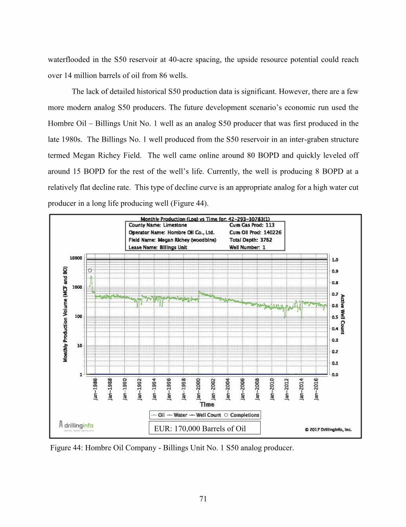
71
waterflooded in the S50 reservoir at 40-acre spacing, the upside resource potential could reach
over 14 million barrels of oil from 86 wells.
The lack of detailed historical S50 production data is significant. However, there are a few
more modern analog S50 producers. The future development scenario’s economic run used the
Hombre Oil – Billings Unit No. 1 well as an analog S50 producer that was first produced in the
late 1980s. The Billings No. 1 well produced from the S50 reservoir in an inter-graben structure
termed Megan Richey Field. The well came online around 80 BOPD and quickly leveled off
around 15 BOPD for the rest of the well’s life. Currently, the well is producing 8 BOPD at a
relatively flat decline rate. This type of decline curve is an appropriate analog for a high water cut
producer in a long life producing well (Figure 44).
Figure 44: Hombre Oil Company - Billings Unit No. 1 S50 analog producer.
EUR: 170,000 Barrels of Oil

72
S50 Economics
The S50 reservoir will require a secondary waterflood program to capture remaining
resources. The OOIP volume of 244 million barrels of oil is encouraging for a development
program because a recovery of a small fraction can result in economics that can be scaled over a
large area of over 3,400 acres. The economic scenario assumes the decline curve of the Billings
Unit No. 1 and EUR of approximately 167,000 barrels of oil. Economic inputs remained the same
as before when the S20 scenario was run: drilling and completion cost per well of $500,000, NRI
of 82.25%, LOE per well of $875 and a flat price of $50 per barrel (Table 3). The resulting
economic run per well is encouraging with a PV10 valuation (present value discounted at 10%) of
$1,533,261. The current economics result in a payout of 26 months and a positive return on
investment. The undiscounted cash flow per well is $5,318,532 throughout the 30-year life of the
producing well. A well such as this represents both a rapid recovery of the initial $500,000
investment and potential for long-term cash flow (Table 5).
If S50 secondary recovery development wells are drilled and are successful, then the
project could be scaled up to fully redevelop the entire Mexia field. Assuming the 3,432 acres to
be redevelopment would be drilled on 40-acre spacings then a total of 83 wells could be drilled.
The capital expenditure for such a project could extend over $41 million, which does not include
any unforeseen expenses. The total upside resources of this project could be over 14 million
barrels of oil with a PV10 value of $131.5 million and an undiscounted cash flow projection of
approximately $456 million (Table 5). Before any drilling and waterflood project occurs in the
S50, reservoir data should be collected and programmed into a waterflooding forecast. A
waterflood engineering firm would be crucial when predicting future economic returns. The S50
waterflood potential in this study is an interpretation of how the economics could be upscaled.
Table 5: Potential upside resources and economics for the S50 Reservoir.
Reservoir
Remaining
Development
Locations
Reserves/well
(barrels of oil)
Total Project
Reserves
(barrels of oil)
PV 10/well
(dollars)
Total Project
PV10 (dollars)
Undiscounted
cash flow/well
(dollars)
Total Project
undiscounted cash
flow (dollars)
S50 86 167,000 14,327,728 1,533,261.00$ 131,545,786.07$ 5,318,532.00$ 456,302,268.60$
Upside Case

73
There are also other secondary recovery options in the S50 sand with high potential. A
prolific reservoir with a strong water drive mechanism would be a candidate for high-volume
pumps such as electric submersible pumps. Even though the percentage of oil produced would be
low, if the well could produce more fluid, then that would mean more oil so long as the produced
water could be reinjected or disposed of efficiently. The waterflood program could also benefit
from chemical injection during the flooding process to help release oil molecules from the
reservoir. The program could also benefit from horizontal drilling where a lateral wellbore would
increase the wellbore exposure to the reservoir and allow a more efficient drainage of the
remaining oil. All of these technologies could, of course, be combined to create the most efficient
secondary recovery effort to produce the largest amount of oil remaining in the Mexia field. These
techniques would require more detailed research and much more data on the reservoir as well as
economic sensitivity cases.

74
Lower S50 and S40 Sandstones
The S50 reservoir mainly consists of completions in the upper sandstone. However, there
are thinner and lower, discontinuous sandstones that are also productive (Figure 45). Historically,
these sandstone units were not developed. There is evidence of only two (2) wells completed in
these lower sandstones. The older S40 depositional cycle includes thin, discontinuous reservoir
sands that were not developed. Although the S40 sands are lower porosity and permeability (18%
porosity), they contain
hydrocarbons and would be a
suitable candidate for hydraulic
fracture stimulation (Figure 45).
These sandstone reservoirs have
tremendous potential, as they are
likely productive between the
trapping fault and the same lowest
known oil (LKO) in the upper S50
reservoir. The reservoir is also
likely to hold virgin pressures since
the upper S50 reservoir is not
connected to lower sandstones.
Figure 45: Brown Oil Co. - H. C. Roller No. K2 log. Type
log of the Upper and Lower S50 Sands and
the S40 Sands.
Upper S50
MFS_S50
MFS_S40
Lower S50
S40 Sands

75
The Lower S50 reservoir net sandstone was not calculated. However, it is estimated that
the sandstone units encompass at least 25 percent of the entire S50 net sandstone thickness (Figure
45). Since the entire depositional
cycle is progradational, the upper
sandstone contains the highest
porosity and permeability (>24%
porosity) and was therefore the
priority target for the operator
(Figure 45). The lower sandstones
have reservoir-quality porosity
and permeability as inferred from
positive production results. The
S40 reservoir sandstones average
10 feet throughout the Mexia field
area and contain some silty
members that could contribute to
production. The area of potential
is equal to approximately 3,432
acres remains to be developed,
with only 2 wells drilled on 20-
acre spacing. There are an
estimated 170 remaining locations
to be drilled on 20-acre spacings to fully develop the lower sandstone units. The Barham lease
(Figure 49) was used as an analog as this lease is the only evidence of lower sandstone completions.
The average per well recovery was 117,000 barrels of oil and could be scaled to future
development of over 19 million barrels of oil, provided full reservoir development.
Figure 46: S40 Net sandstone map zoomed into the Mexia
field. Average net sand thickness throughout
the Mexia field is 10 feet. Purple polygon
indicates potential Lower S50 and S40 sand
productive reservoir; 3,432 acres.
Lower S50
and S40
Potential
Reservoir
Barham
Lease
Well

76
The Barham lease is located in the northern half of the Mexia field and began producing in
1960, long after the field was thought to have been depleted. The Barham No. 1 well was drilled
and completed in June 1960 with the No. 2
well following in October 1960. The No. 1
well perforated the S40 section from 3,126-
3,180 feet and initially pumped 125 barrels of
fluid per day with 99 percent being saltwater
(Figure 47). The operator continued pumping
the reservoir and by June 23, 1960, just 14 days
after initial testing, the well had begun
producing more oil. The operator reached a
leveled-pumping volume of 53 BOPD and 123
BWPD. This is significant because there is no
other evidence of an operator producing from
the S40 sandstones. Subsequently, the operator
completed the No. 2 well in the Lower S50
sandstones (Figure 48). They perforated
3,078-79 feet and brought it into production
pumping at 14 BOPD and 126 BWPD on
October 11, 1960 (www.drillinginfo.com,
2017). The Barham lease is commingled
production at the surface and reported together.
Therefore, an average per-well rate is the best
assumption to make. The lease produced
233,197 barrels of oil from 1960 through 1992
from the No. 1 and No. 2 wells, which averages approximately 117,000 barrels of oil per well
Figure 47: Texas Alberta Oil - Barham No. 1
well log. Completed 6/23/1960.
Perforated: 3,126-80'.
3126-80’
Figure 48: Texas Alberta Oil - Barham No. 2
well log. Completed 10/11/1960.
Perforated: 3,078-79'.
3,078-79’

77
(Figure 49). The two wells provide the evidence of a potentially significant amount of bypassed
resources that were overlooked during initial development of the field.
Lower S50 and S40 Economics
The Lower S50 and S40 sandstone reservoirs were predicted to have an EUR of 117,000
barrels of oil per well. The sandstones are assumed to be commingled in one down-hole completion
for a single EUR per well due to the absence of detailed completion and production data. An
economic scenario was performed using the Barham lease and the same economic inputs for the
other reservoirs were analyzed in the report, assuming drilling and completion cost per well of
$500,000, NRI of 82.25 percent, LOE of $875 per well and a flat price of $50 per barrel (Table 3).
Figure 49: Production curve for the Barham No. 1 and No. 2 wells. Analog production for the
Lower S50 and S40 sandstones.

78
Payout of the initial drilling investment would occur within 31 months and positive return on
investment. The PV10 is calculated to be $1 million per well and an undiscounted cash flow of
over $4 million per well. Similar to the prior economic scenarios, the present value of a Lower
S50 well is significantly less than the potential future cash flow because of the long-life nature of
the well’s production. Most of the well’s value is weighted in the long-term cash flow rather than
the initial payback of the investment. If full development of the field were to occur, 170 wells
could be drilled for a PV10 value of over $191 million and an undiscounted cash flow of over $709
million (Table 6). To reach this potential upside revenue, an initial capital expenditure of $84.5
million would be necessary to drill and produce. Future infrastructure was not considered in this
economic scenario and may be necessary. If S40 sandstones require hydraulic fracture stimulation,
an updated economic scenario would also be required. However, based on current economics,
those potential cost overages would not greatly affect the potential revenue from the Lower S50
and S40 development plans.
S70 Sandstone
S70 reservoir sandstones in the Mexia field are also known as the stringer sands. The
stringer sands were penetrated in wells drilled to the S50. Therefore, many of the wells had a
preview of the S70 sandstones and their potential. The S70 is known to be productive throughout
the entire Mexia field area and is currently being pumped in multiple wells that are still producing
(Figure 50). There were even some wells drilled specifically to produce S70 sandstones.
Therefore, there is less upside potential since the reservoir has been previously developed.
Table 6: Upside potential economics and resources for the Lower S50 and S40 reservoirs.
Reservoir
Remaining
Development
Locations
Reserves/well
(barrels of oil)
Total Project
Reserves
(barrels of oil)
PV 10/well
(dollars)
Total Project PV10
(dollars)
Undiscounted
cash flow/well
(dollars)
Total Project
undiscounted cash
flow (dollars)
Lower S50 170 116,500 19,757,183 1,128,708.00$ 191,417,087.04$ 4,185,241.00$ 709,773,157.24$
Upside Case

79
The S70 reservoir is
known to be productive
downdip of the trapping fault
and updip to the S50 LKO
structural contour. In
addition, the southern portion
of the field the S70 is even
known to produce downdip
of the LKO mark. An
average of 20 feet of net
sandstone is present in the
S70 depositional cycle
throughout the Mexia field.
Historically, there have been
60 wells that appear to have
produced from the S70
reservoir based on their
perforated interval.
According to the Texas
Railroad Commission the
wells drain 20 acres and,
therefore there is potential for 115 future wells to be drilled. If all of the 115 development locations
were to be drilled, an upside case of over 9.4 MMBO could be achieved. The Brown Oil and Gas
Company - Freeman No. 1 well was used as an analog since it was drilled in 1957, after the initial
discovery of the field. It was an appropriate analog because it serves as a well that could potentially
have a lower reservoir pressure since many wells have been drilled in the S70 reservoir before
production.
Figure 50: S70 Net sandstone map zoomed into the Mexia field.
Average net sand thickness throughout the Mexia
field is ~20 feet. Purple polygon indicates potential
S70 sand productive reservoir; 3,493 acres.
Down-dip
S70 Producers
Freeman No. 1
Freeman No. 1
S70 Potential
Reservoir

80
Many of the historical Mexia leases were commingled and many wells in each lease
produced concurrently from the S50 and the S70 reservoirs. The absence of definitive data restricts
assigning resources to the S70 sandstones; therefore, the Freeman No. 1 well was used because it
was produced on a one (1) well lease for the entirety of the economic life of the well. It also serves
as a conservative analog since it was drilled later in the field’s history and has a higher possibility
of depletion. The Freeman No. 1 well produced 82,000 barrels of oil and if the resources per well
were attributed to the prior 60 wells, then the wells can be attributed approximately 4.9 MMBO of
the Mexia field’s cumulative production (Figure 51). The S70 reservoir is estimated to have
produced 4.5 percent of the total field reserves to date with the potential of growing as S70 wells
continuing to produce in the future.
Figure 51: Brown Oil and Gas Company - Freeman No. 1 monthly production curve.

81
There are multiple examples of the S70 reservoir producing currently at flat decline rates
with potential to continue producing for decades. The S70 stringer sand reservoirs tend to pump
low volumes of oil at low decline rates for long periods of time. For instance, the Freeman No. 1
well produced between 200 and 300 barrels of oil per month (6-10 BOPD) for over 30 years before
it began declining (Figure 51). Another well, The C. A. Kennedy No. 1, has been producing since
1938 from the S70 reservoir. Although the well’s production volumes have varied, they eventually
leveled out and since 1987 the production has been consistent at 20 BOPD with no noticeable
decline rate (Figure 52). The well
has produced a cumulative
volume of 312,545 barrels of oil
since 1938. Brown Oil and Gas
Company recently drilled a new
S70 well on the H. C. Roller lease
and brought the well online at 6
BOPD with a slight decline rate.
It is possible that the Roller No.
K2 will have a similar production
curve because of the flat decline
rate. It is evident that the S70
reservoir has remaining oil in the reservoir that has high potential for future development.
S70 Economics
An economic scenario was created using the Freeman No. 1 decline curve analog (Figure
51) and a per-well recovery of 82,000 barrels of oil. The economic inputs were the same used in
the prior economic scenarios, namely drilling and completion cost per well of $500,000, NRI of
82.25 percent, LOE of $875 per well and a flat price of $50 per barrel (Table 3). Since the analog
well is a low volume, long life producers it is expected that the payout is 68 months, however the
Figure 52: Brown Oil and Gas Company - C. A. Kennedy No.
1 decline curve. Daily production volume, S70
reservoir.
20 BOPD

82
ROI is positive. Although it does not payout quickly, the investment has a lower risk profile since
there is proven production in the S70 reservoir. The PV10 valuation is $330,000 per well and an
undiscounted cash flow of over $2 million. This does not seem significant. However, if 115 low
risk development locations can be drilled then it can be scaled substantially. If all 115 wells were
to be drilled the PV10 could be scaled to $37.9 million and the undiscounted cash flow could reach
over $234 million (Table 7).
CUMULATIVE ECONOMICS OF FUTURE DEVELOPMENT
The Mexia field has many reservoirs with future development potential. These reservoirs
have been overlooked in the past because operators were focused solely on high flow rates of the
‘Main Pay’ S50 reservoir. Future development can be achieved primarily through infill drilling of
previously undeveloped reservoirs within the original the Mexia field area but also through
secondary recovery efforts in the original S50 reservoir unit. The capital-intensive nature of
drilling and completing wells requires that the economics of each reservoir be vetted prior to future
development. Therefore, each reservoir’s economic scenario assumed that a well would be drilled
specifically to produce resources in that reservoir only.
The current economic scenarios can be summed up to find a total project present value and
undiscounted cash flow value. This assumes that all development wells are drilled and each
development location completes just one reservoir unit. The total number of development
locations would be 474 new wells, which would equate to $237 million in cost. An estimated 51.2
MMBO could be produced from this investment, roughly one-half of the Mexia field’s historical
cumulative production (Table 8). The produced resources would be a long-term investment and
depending on future oil commodity prices, then the economics of the project could vary
Table 7: Potential upside resources and economics for the S70 Reservoir.
Reservoir
Remaining
Development
Locations
Reserves/well
(barrels of oil)
Total Project
Reserves
(barrels of oil)
PV 10/well
(dollars)
Total Project PV10
(dollars)
Undiscounted
cash flow/well
(dollars)
Total Project
undiscounted cash
flow (dollars)
S70 115 82,057 9,407,193 329,606.00$ 37,786,747.65$ 2,038,255.00$ 233,669,979.71$
Upside Case

83
significantly. At a flat $50 oil price the PV10 of the development project would be a cumulative
of over $411 million. The cumulative undiscounted cashflow would equate to over $1.6 billion
(Table 8).
Given the upside cashflow and present value, $237 million to drill 474 wells is a significant
amount of money to allocate to a mature oil field. There are techniques to save costs that could
substantially reduce the cost per well by commingling multiple reservoir completions in one
wellbore. The initial $500,000 drilling and completions cost could be spread over two or possibly
three reservoir completions. The reduced capital expenditure would drastically increase the
economic and valuation indicators. Return on investment would increase and the payout timeframe
would be reduced. Since the reservoirs are a long-term investment, the lower upfront costs would
greatly benefit the development of the field. Reducing costs would potentially increase the
resources to be produced because it could change the economics enough to encourage drilling
where a well otherwise would not be drilled.
If future development were to occur in the Mexia field, engaging a drilling and completions
engineering firm would be encouraged to help reduce costs. Streamlining an operation such as
drilling 474 wells could be the difference between drilling uneconomic producers and earning a
significant ROI. Nonetheless, the Mexia field retains untapped potential of over 51 million barrels
of oil and deserves to be closely examined at current or higher commodity.
APPLICATION IN OTHER WOODBINE FIELDS
Along strike to the north of the Mexia field are other Woodbine fields with trapped oil
along similar salt-withdrawal graben structures. The fields to the north are closer to the Woodbine
Table 8: Potential upside resources and economics for all Mexia field reservoirs.
Reservoir
Remaining
Development
Locations
Reserves/well
(barrels of oil)
Total Project
Reserves
(barrels of oil)
PV 10/well
(dollars)
Total Project PV10
(dollars)
Undiscounted
cash flow/well
(dollars)
Total Project
undiscounted cash
flow (dollars)
S20 100 73,941 7,422,268 471,851.25$ 47,364,636.45$ 2,010,091.00$ 201,773,820.57$
S70 115 82,057 9,407,193 329,606.00$ 37,786,747.65$ 2,038,255.00$ 233,669,979.71$
S50 86 167,000 14,327,728 1,533,261.00$ 131,545,786.07$ 5,318,532.00$ 456,302,268.60$
Lower S50 173 116,500 20,112,813 1,128,708.00$ 194,862,600.35$ 4,185,241.00$ 722,549,095.40$
Upside Case

84
sediment source and therefore have thicker and more numerous of sandstone reservoirs. Similar
to the Mexia field, these fields were discovered in the 1920s and have not had detailed geological
studies performed on reservoir units. The fields were also thought to be produced at such high
flow rates that there are significant resources remaining in the reservoirs. The Powell field had
approximately 259 million barrels of OOIP (Galloway et al., 1983). The Wortham field is less,
although significant with 59 million barrels of OOIP. The two fields were estimated to only have
produced between 45 and 51 percent of the OOIP. The Currie and Richland fields have much
smaller volumes of OOIP but would also benefit from this type of study. It is estimated by Tyler
et al. (1984) that approximately 199 million barrels of mobile oil remain in the Mexia Fault Trend.
The type of research study presented here should be applied to all of the Mexia Fault Trend
fields. The amount of remaining recoverable upside resources in the Mexia field are over 51
MMBO, which is roughly 21 percent of the OOIP. If the same volumetric could be realized in the
Powell and Wortham fields, then a potential of approximately 67 MMBO could be produced.
A 3D seismic survey should also be coupled with the detailed field studies for each
structural trap in the trend. None of the major fields in the Mexia Fault Trend have been mapped
with 3D seismic data. The structural complexities of the fields would be better understood with
3D imaging. Since high-resolution subsurface geophysical data was not gathered during initial
field development, the seismic would fill in gaps to enhance a potential future development project.
The new survey would also be beneficial in targeting undrained fault blocks and inter-graben
trapping structures. Overall, any 3D seismic data that is acquired would offer significant new
information for any studies in the Mexia Fault Trend.

85
Conclusions
The Woodbine Group’s depositional systems in the study area are summarized below.
➢ The S20 depositional cycle is interpreted to be fluvial-dominated delta in origin. It
was moderately influenced by wave reworking.
➢ The S30 depositional cycle was interpreted to be a fluvial dominated delta in origin.
There appears to be no influence of wave reworking. The study area is interpreted
to be located within the distal prodelta region of the deltaic system.
➢ The S40 depositional cycle is interpreted as a wave-dominated delta in origin with
moderate fluvial influence.
➢ The S50 depositional cycle is interpreted as a fluvial-dominated delta in origin with
moderate wave influence.
➢ The S60 depositional cycle is interpreted as a fluvial-dominated delta in origin.
➢ The S70 depositional cycle is interpreted as a fluvial-dominated delta in origin.
➢ The S80 and S90 depositional cycles are interpreted as prodelta and offshore muddy
facies.
The Mexia field’s production history and future production potential is summarized below.
➢ Cumulative oil production is 110,387,637 barrels of oil from 659 oil wells as of
December 31, 2016.
➢ The EUR is calculated to be approximately 112,000,000 barrels of oil, which
equates to approximately 46 percent of the OOIP. This EUR assumes that no future
redevelopment is to occur.
➢ Numerous infill development wells could be drilled that could lead to upside
potential resources.
➢ The S20 sandstone reservoirs have potential to produce 7.4 million barrels of oil
with a PV10 value of over $47,000,000.

86
➢ The S70 sandstone reservoirs have potential to produce to 9.4 million barrels of oil
with a PV10 value of over $37,000,000.
➢ The S50 sandstone reservoirs have potential to produce 14.3 million barrels of oil
with a PV10 value of over $131,000,000.
➢ The lower S50 sandstone reservoirs have potential to produce 20.1 million barrels
of oil with a PV10 value of over $191,000,000.
➢ Cumulative redevelopment resources equate to 51.3 million barrels of oil with a
PV10 value of over $411,000,000.
➢ Cumulative EUR for the Mexia field is 163.3 million barrels of oil.

87
References
Ambrose, W.A., Breton, B., Nunez-Lopez, V., Gulen, G., 2015, EOR potential from CO2 captured
from coal-fired power plants in the Upper Cretaceous (Cenomanian) Woodbine Group,
East Texas Basin, and Southeastern Texas Gulf Coast, USA, Natural Resources Research,
v. 24, no. 2, p. 161-188, doi 10.1007/s11053-014-9242-z.
Ambrose, W. A., Hentz, T. F., Bonnaffe, F., Loucks, R. G., Brown, L. F., Wang, F. P., Potter, E.
C., 2009, Sequence-stratigraphic controls on complex reservoir architecture of highstand
fluvial-dominated deltaic and lowstand valley-fill deposits in the Upper Cretaceous
(Cenomanian) Woodbine Group, East Texas field: Regional and local perspectives, AAPG
Bulletin, v. 93, no. 2, p. 231-269.
Anonymous, 1947, J. K. Hughes Oil Company Mexia field history: excerpt provided to Carl Coke
Rister, Research Professor, The University of Oklahoma, 30 p.
Blakey, R. C., 2014, Paleogeography and paleotectonics of the Western Interior Seaway, Jurassic-
Cretaceous of North America, AAPG Search and Discovery Article #30392.
Boyd, R., Dalrymple, R., Zaitlin, B. A., 1992, Classification of clastic depositional environments,
Sedimentary Geology, 80, p. 139-150.
Bunge, R. J., 2011, Woodbine Formation sandstone reservoir prediction and variability, Polk and
Tyler Counties, Texas, AAPG Search and Discovery Article #10331.
Corbett, K., Friedman, M., Spang, J., 1987, Fracture development and mechanical stratigraphy of
Austin Chalk, Texas, AAPG Bulletin, v. 71, no. 1, p. 17-28.
Dokur, M., 2012, Reservoir characterization of the Upper Cretaceous Woodbine Group in
Northeast East Texas Field, Texas, Master of Science in Geological Sciences, The
University of Texas at Austin, Austin, 98 p.
Dokur, M., Hentz, T. F., 2012, Reservoir characterization of the Upper Cretaceous Woodbine
Group in Northeast East Texas Field, Texas, AAPG Search and Discovery Article #20152.
Fisher, W. L., Brown, L. F., Jr., Scott, A. J., and McGowen, J. H., 1969, Delta systems in the
exploration for oil and gas: The University of Texas at Austin, Bureau of Economic
Geology Research Colloquium, variously paginated.
Foote, R. Q., Massingill, L. M., Wells, R. H., 1988, Petroleum geology and the distribution of
conventional crude oil, natural gas, and natural gas liquids, East Texas Basin, Department
of the Interior, U.S.G.S. Open File Report 88-450K.
Galloway, W.E., 1975. Process framework for describing the morphologic and stratigraphic
evolution of deltaic depositional systems, in deltas, M.L. Broussard, ed., Houston
Geological Society, 87-98.
Galloway, W.E., Ewing, T. E., Garrett, C. M., Tyler, N., Bebout, D. G., 1983, Atlas of major Texas
oil reservoirs, Bureau of Economic Geology, 139 p.
Hager, D. S., Burnett, C. M., 1960, Mexia-Talco fault line in Hopkins and Delta Counties, Texas,
AAPG Bulletin, v. 44, no. 3, p. 316-356.

88
Hammes, U., Hamlin, H.S., Ewing, T.E., 2011, Geologic analysis of the Upper Jurassic
Haynesville Shale in East Texas and West Louisiana, AAPG Bulletin, v. 95, no. 10, p.
1643-1666.
Hansen, K. L., Verhyden, M.S., 1991, Benefits of a horizontal well in a sandstone waterflood: a
case study, Society of Petroleum Engineers Rocky Mountain Regional Meeting, SPE
24370.
Haq, B. U., 2014, Cretaceous eustasy revisited, Global and Planetary Change, v. 113, p. 44-58.
Haq, B. U., Harendol, J., Vail, P.R., 1987, Chronology of fluctuating sea levels since the Triassic,
Science, v. 235, no. 4793, p. 1156-1167.
Hentz, T.F., Ambrose, W.A., Smith, D.C., 2014, Eaglebine play of the southwestern East Texas
basin: Stratigraphic and depositional framework of the Upper Cretaceous (Cenomanian-
Turonian) Woodbine and Eagle Ford Groups, AAPG Bulletin, v. 98, no. 12, p. 2551-2580,
doi 10.1306/07071413232.
Hentz, T. F., Ruppel, S. C., 2001, Regional stratigraphic and rock characteristics of Eagle Ford
Shale in its play Area: Maverick Basin to East Texas Basin, AAPG Search and Discovery
Article #10325.
Hill, H. B., and Guthrie, R. K., 1943, Analysis of oil production in the near-depleted Mexia-Powell
Faultline fields of Texas, United States Department of the Interior, Report of Investigations
No. 3712, 83 p.
Hovorka, S. D., 1998, Facies and diagenesis of the Austin Chalk and controls on fracture intensity
– a case study from north-central Texas, Bureau of Economic Geology, Geological Circular
98-2, 47 p.
Jackson, M. P. A., 1982, Fault tectonics of the East Texas Basin, Bureau of Economic Geology,
Geological Circular 82-4.
Mancini, E. A., and Pucket, T. M., 2005, Jurassic and Cretaceous transgressive-regressive (T-R)
cycles, northern Gulf of Mexico, USA, Stratigraphy, V. 2, no. 1, p. 31-48.
Oliver, W. B., 1971, Depositional systems in the Woodbine Formation (Upper Cretaceous),
Northeast Texas, Bureau of Economic Geology, Report of Investigations No. 73, 28 p.
Pearson, O. N., Rowan, E. L., Miller, J. J., 2012, Modeling the Mesozoic-Cenozoic structural
evolution of East Texas, GCAGS Journal, v. 1, p. 118-130.
Salvador, A., 1991, Origin and development of the Gulf of Mexico Basin: Geological Society of
America, Decade of North American Geology, V. J, p. 389-444.
Seni, S. J., Jackson, M. P. A., 1984, Sedimentary record of Cretaceous and Tertiary salt movement,
East Texas Basin: times, rates, and volumes of salt flow and their implications for nuclear
waste isolation and petroleum exploration, Bureau of Economic Geology Report of
Investigations No. 139, 89 p.
Tyler, N., Galloway, W. E., Garrett, Jr., C. M., Ewing, T. E., 1984, Oil accumulation, production
characteristics, and targets for additional recovery in major oil reservoirs of Texas, Bureau
of Economic Geology Geologic Circular 84-2, 31 p.

89
Wang, F. P., 2010, Engineering characterization of East Texas oil field: north and south pilot
studies, Bureau of Economic Geology Special Publication, p. 95-114.
Weber, K.J., Dronkert, H., 1999, Screening criteria to evaluate the development potential of
remaining oil in mature fields, SPE European Petroleum Conference, SPE 57873.
Wescott, W. A., Hood, W. C., 1994, Hydrocarbon generation and migration routes in the East
Texas Basin, AAPG Bulletin, v. 78, no. 2, p. 287-307.