Copyright

by

Dale Wilson Fox III

2018

The Thesis Committee for Dale Wilson Fox III

Certifies that this is the approved version of the following thesis:

Experiments and Simulation of Shaped Film Cooling Holes Fed by

Crossflow with Rib Turbulators

APPROVED BY

SUPERVISING COMMITTEE:

David G. Bogard

Vaibhav Bahadur

Supervisor:

Experiments and Simulation of Shaped Film Cooling Holes Fed by

Crossflow with Rib Turbulators

by

Dale Wilson Fox III

Thesis

Presented to the Faculty of the Graduate School of

The University of Texas at Austin

in Partial Fulfillment

of the Requirements

for the Degree of

Master of Science in Engineering

The University of Texas at Austin

May 2018

Dedication

To my parents, to whom I owe everything.

v

Acknowledgements

I would first like to thank Dr. David Bogard, for his vast wisdom and guidance

through my journey through graduate school. I also would like to thank the other members

of the TTCRL- Dr. Josh Anderson, Dr. John McClintic, Jabob Moore, Chris Yoon, Fraser

Jones, and Khanh Hoang- for their assistance, guidance, and friendship as I worked on my

master’s degree here at UT. Here’s to all the Taco Tuesdays.

Additionally, all my close friends from KU- Kyle Strickland, Madison Outlaw,

McKinzey Manes, Michael Zeets, Dan Smith, Amanda Katzer, Harrison Hetler- I cannot

overstate how much your friendship means to me. Thank you all for sticking together even

as we move apart.

This work was supported by GE Aviation, and I am grateful for the input from Dr.

Tom Dyson and Zach Webster on this work.

Finally, my brother, mom, and dad, for their continual love and support. I couldn’t

have asked for better family.

vi

Abstract

Experiments and Simulation of Shaped Film Cooling Holes Fed by

Crossflow with Rib Turbulators

Dale Wilson Fox III, M.S.E.

The University of Texas at Austin, 2018

Supervisor: David G. Bogard

Most studies of turbine airfoil film cooling in laboratories have used relatively large

plenums to feed flow into the coolant holes. A more realistic inlet condition for the film

cooling holes is an internal crossflow channel. In this study, angled rib turbulators were

installed in two geometric configurations inside the internal crossflow channel, at 45° and

135°, to assess the impact on film cooling effectiveness. Film cooling hole inlets positioned

in both pre-rib and post-rib locations tested the effect of hole inlet position relative to the

rib turbulators. Experiments were performed varying channel velocity ratio and jet to

mainstream velocity ratio. These results were compared to the film cooling performance

of previously measured shaped holes fed by a smooth internal channel, as well as RANS

simulations performed for select cases. The film cooling hole discharge coefficients and

channel friction factors were measured for both rib configurations. Spatially-averaged film

cooling effectiveness behaves similarly to holes fed by a smooth internal crossflow

channel, but hole-to-hole variation due to the obstruction by the ribs was observed.

vii

Table of Contents

List of Tables ......................................................................................................... ix

List of Figures ..........................................................................................................x

Chapter 1: Introduction ............................................................................................1

1.1 – Gas Turbine Cooling ..............................................................................1

1.2 – Experimental Film Cooling Measurement .............................................3

1.3 – Adiabatic Effectiveness of Plenum Fed Holes.......................................6

1.4 – Crossflow Effect on Adiabatic Effectiveness ........................................7

1.5 – Effects of Rib Turbulators in Internal Channels ....................................8

1.6 – Simulation of Film Cooling .................................................................10

1.7 – Objectives of the Present Study ...........................................................13

Chapter 2: Experimental Methods ........................................................................14

2.1 - Experimental Facilities .........................................................................14

2.1.1 – Mainstream Flow Loop ............................................................14

2.1.2 – Coolant Flow Loop ..................................................................17

2.1.3 – Summary of Test Conditions ...................................................20

2.2 – Data Acquisition And Analysis ...........................................................21

2.2.1 – Pressure and Temperature Measurement .................................21

2.2.2 – IR Thermography .....................................................................23

2.3 – Data Reduction.....................................................................................25

2.4 – Uncertainty Analysis ............................................................................28

2.4.1 – Precision Uncertainty and Repeatability ..................................28

2.4.2 – Flowrate Uncertainty ...............................................................31

2.4.3 – Discharge Coefficient Uncertainty ..........................................32

2.4.4 – Friction Factor Uncertainty ......................................................33

2.4.5– Adiabatic Effectiveness Uncertainty.........................................34

Chapter 3: Computational Methods .......................................................................35

3.1 – Rans Simulation Method......................................................................35

3.1.1 – Turbulence Closure ..................................................................36

viii

3.1.2 – Wall Functions .........................................................................38

3.1.3 – Thermal Transport ...................................................................39

3.3 – Boundary Conditions and Adjunct Simulations ..................................39

3.4 – Grid Generation ...................................................................................45

3.5 – Convergence Criteria ...........................................................................47

Chapter 4 – Experimental Results for Rib Turbulator Crossflow-Fed Film Cooling

Holes .............................................................................................................49

4.1 – Film Cooling hole discharge coefficients ............................................49

4.2 – Channel Friction Factor .......................................................................53

4.3 – Adiabatic Film Cooling Effectiveness .................................................55

4.3.1 Pre- and Post-Rib Variation of Adiabatic Effectiveness .............60

Forward Deflecting Rib Crossflow-fed Film Cooling Holes ......60

Backward Deflecting Rib Crossflow-fed Film Cooling Holes ...64

4.3.2 – Jet Bias Parameters of Adiabatic Effectiveness .......................66

Chapter 5: Computational Results .........................................................................72

5.1 – Film Cooling Hole Discharge Coefficient ...........................................72

5.2 – Adiabatic Film Cooling Effectiveness .................................................73

5.2.1 – Effectiveness of Forward Deflecting Rib-Fed Holes ...............74

5.2.2 – Effectiveness of Backward Deflecting Rib-Fed Holes ............77

Chapter 6: Conclusions ..........................................................................................80

6.1 – Summary ..............................................................................................80

6.2 – Recommendations for Future Work .....................................................82

References ..............................................................................................................83

Vita... ......................................................................................................................86

ix

List of Tables

Table 1: Mainstream operating conditions ............................................................21

Table 2: Crossflow and jet parameters tested ........................................................21

x

List of Figures

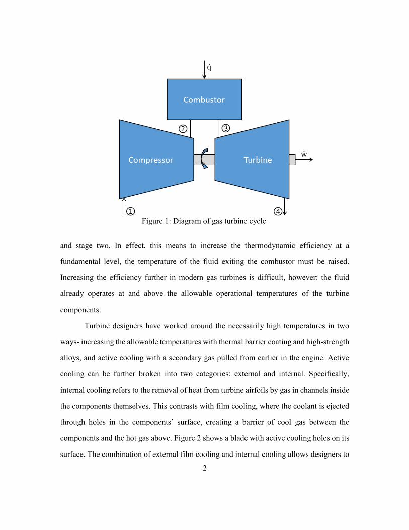
Figure 1: Diagram of gas turbine cycle ....................................................................2

Figure 2: Example modern gas turbine blade [1].....................................................3

Figure 3: Low speed wind tunnel diagram ............................................................15

Figure 4: Test section and crossflow channel diagram ..........................................16

Figure 5: Boundary layer measurement from [24] ................................................16

Figure 6: Coolant channel rib turbulator configuration diagram ...........................19

Figure 7: Shaped hole geometry from [25] ............................................................19

Figure 8: Adiabatic effectiveness of the repeated measurement at VR = 1.11 and VRc

= 0.3 ..................................................................................................30

Figure 9: Diagram of the primary computational domain .....................................40

Figure 10: Boundary layer velocity profile from 2D adjunct simulation (a) scaled with

inner coordinates (b) scaled by inlet velocity and cooling hole diameter.

...........................................................................................................42

Figure 11: Rib turbulated channel geometry for the adjunct simulation ...............43

Figure 12: Velocity and turbulent kinetic energy contours for the channel adjunct

simulations ........................................................................................44

Figure 13: Mesh generated for film cooling simulation by ICEM ........................46

Figure 14: Scaled residuals for VRc = 0.4, VR = 1.11 (a) backward-deflecting rib

configuration and (b) forward-deflecting rib configuration ..............48

Figure 15: Discharge coefficients for film cooling holes fed by crossflow. Lines

indicate trends at constant VR. .........................................................50

Figure 16:Scaling discharge coefficient with (a) average and (b) inlet channel velocity

...........................................................................................................52

xi

Figure 17: Channel friction factor for different rib and smooth channel configurations

...........................................................................................................54

Figure 18: Spatially averaged adiabatic effectiveness for (a) forward deflecting rib-

fed (b) backward deflecting rib-fed and (c) smooth channel- and

plenum-fed film cooling holes ..........................................................56

Figure 19: Spatially averaged effectiveness, compared for varying channel

configuration .....................................................................................57

Figure 20: Spatially averaged adiabatic effectiveness, scaled with inlet velocity ratio,

for (a) forward deflecting rib-fed (b) backward deflecting rib-fed and (c)

smooth channel-fed film cooling holes. ............................................59

Figure 21: Spatially averaged effectiveness pre- and post-rib variation for forward

deflecting rib-fed holes .....................................................................60

Figure 22: Contours of forward deflecting rib-fed shaped hole effectiveness .......61

Figure 23: Comparison of effectiveness at VR = 0.28 for forward- and backward-

deflecting rib-fed holes .....................................................................63

Figure 24: Spatially averaged effectiveness comparison between (a) pre-rib and (b)

post-rib positioned holes ...................................................................64

Figure 25: Spatially averaged effectiveness pre- and post-rib variation for backward

deflecting rib-fed holes .....................................................................65

Figure 26: Contours of backward deflecting rib-fed shaped hole effectiveness ....66

Figure 27: Centerline location for (a) pre-rib and (b) post-rib film cooling holes fed

by a channel with forward deflecting ribs.........................................67

Figure 28: Centerline location for (a) pre-rib and (b) post rib film cooling holes fed by

a backward deflecting ribbed channel ...............................................69

xii

Figure 29: Centerline location scaled with VR for (a) pre-rib holes fed by a channel

with forward deflecting ribs, (b) post-rib holes fed by a channel with

forward deflecting ribs (c) holes fed by smooth channel ..................70

Figure 30: Centerline location scaled with VR for (a) pre-rib holes fed by a channel

with backward deflecting ribs, (b) post-rib holes fed by a channel with

backward deflecting ribs (c) holes fed by smooth channel ...............71

Figure 31: Simulated discharge coefficient compared with experiment for VRc = 0.4

...........................................................................................................73

Figure 32: Contours of effectiveness for forward deflecting rib crossflow-fed holes, at

a VRc = 0.4 ........................................................................................74

Figure 33: Adiabatic effectiveness of film cooling holes fed by forward deflecting rib

crossflow, for pre- and post-rib holes. VRc = 0.4 ..............................75

Figure 34: Adiabatic effectiveness of film cooling holes fed by backward deflecting

rib crossflow, for pre- and post-rib holes. VRc = 0.4 ........................76

Figure 35: Adiabatic effectiveness of film cooling holes fed by forward deflecting rib

crossflow, for pre- and post-rib holes. VRc = 0.4 ..............................77

Figure 36: Contours of effectiveness for backward deflecting rib crossflow-fed holes

...........................................................................................................79

1

Chapter 1: Introduction

1.1 – GAS TURBINE COOLING

Gas turbines are a cornerstone of the modern power generation and transportation

industries. For their ability to handle variable load with high efficiency and use cheap

natural gas as fuel, they are popular as generators of electricity for the grid. With small

form factors and high power, they are the only engine in use in commercial freight and

passenger planes. The basis of gas turbine operation is the Brayton cycle. As shown in

Figure 1, the Brayton cycle operates through three sequential processes: compression, heat

addition in the combustor, and expansion. Air is brought from outside into the compressor,

which brings it to a high pressure. Within the combustor, fuel is added and burned,

increasing the temperature. Work is extracted from the fluid in the turbine, lowering the

temperature and pressure. It is then exhausted back to the atmosphere. Some of this

extracted work is used to drive the compressor, but the majority is usable power for

electricity generation or aircraft thrust.

In this idealized Brayton model, the thermal efficiency of the cycle – the amount of

heat released by the combustion that is turned into usable work – is determined by the

operation temperatures between each of the stages. This is shown by the Brayton cycle

thermal efficiency:

𝜂𝑡ℎ = 1 −𝑇4 − 𝑇1

𝑇3 − 𝑇2

The subscripted temperatures are those of the inter-component stages in Figure 1. While

there is little control over the inlet temperature of the cycle, the efficiency can be increased

if the fraction is made smaller, by increasing the temperature difference between stage three

2

and stage two. In effect, this means to increase the thermodynamic efficiency at a

fundamental level, the temperature of the fluid exiting the combustor must be raised.

Increasing the efficiency further in modern gas turbines is difficult, however: the fluid

already operates at and above the allowable operational temperatures of the turbine

components.

Turbine designers have worked around the necessarily high temperatures in two

ways- increasing the allowable temperatures with thermal barrier coating and high-strength

alloys, and active cooling with a secondary gas pulled from earlier in the engine. Active

cooling can be further broken into two categories: external and internal. Specifically,

internal cooling refers to the removal of heat from turbine airfoils by gas in channels inside

the components themselves. This contrasts with film cooling, where the coolant is ejected

through holes in the components’ surface, creating a barrier of cool gas between the

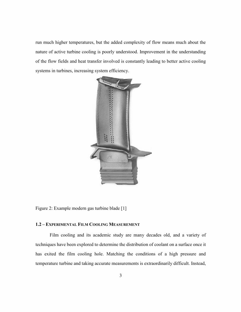
components and the hot gas above. Figure 2 shows a blade with active cooling holes on its

surface. The combination of external film cooling and internal cooling allows designers to

Figure 1: Diagram of gas turbine cycle

3

run much higher temperatures, but the added complexity of flow means much about the

nature of active turbine cooling is poorly understood. Improvement in the understanding

of the flow fields and heat transfer involved is constantly leading to better active cooling

systems in turbines, increasing system efficiency.

1.2 – EXPERIMENTAL FILM COOLING MEASUREMENT

Film cooling and its academic study are many decades old, and a variety of

techniques have been explored to determine the distribution of coolant on a surface once it

has exited the film cooling hole. Matching the conditions of a high pressure and

temperature turbine and taking accurate measurements is extraordinarily difficult. Instead,

Figure 2: Example modern gas turbine blade [1]

4

geometric, dynamic, and kinematic similarity with engine conditions is met by matching

the governing non-dimensional groups, such that the expected behavior is the same.

Geometric similarity is achieved by scaling up the relevant geometry of a turbine

airfoil to sizes testable in the lab. However, a commonly used simplification of the

geometry in laboratory environments violates the geometric similarity assumption: the

feeding of film cooling holes with a plenum. In reality, the flow into the hole is not uniform,

plenum-like flow directly up toward the film cooling hole from below. Turbines use

internal channels, impingement jets, and other internal flow configurations to enhance the

internal cooling of the components. These internal flows mean that the coolant fed into the

holes has significant transverse velocity component, which has been shown to affect the

path of the coolant as it exits the hole. Therefore, for true geometric similarity, the internal

passages must be scaled appropriately.

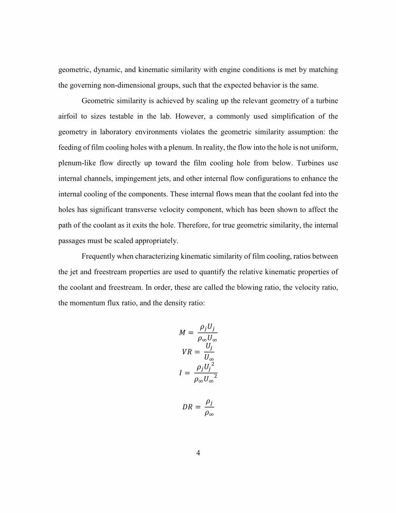
Frequently when characterizing kinematic similarity of film cooling, ratios between

the jet and freestream properties are used to quantify the relative kinematic properties of

the coolant and freestream. In order, these are called the blowing ratio, the velocity ratio,

the momentum flux ratio, and the density ratio:

𝑀 = 𝜌𝑗𝑈𝑗

𝜌∞𝑈∞

𝑉𝑅 = 𝑈𝑗

𝑈∞

𝐼 = 𝜌𝑗𝑈𝑗

2

𝜌∞𝑈∞2

𝐷𝑅 = 𝜌𝑗

𝜌∞

5

The blowing ratio is a measure of the relative mass flux of coolant through the hole.

Therefore, the effectiveness generally increases with increasing M. VR is indicative of the

strength of the shear layer between the jet and the freestream, and hence is tied to the

strength of the mixing action that the freestream has on the jet. I is a ratio of the momentum

carried by the jet and freestream. For all film cooling holes, there is a point (as I increases)

where the adiabatic effectiveness begins to decrease. This point is where the wall-normal

momentum of the jet is high enough that the freestream can no longer push the jet toward

the wall, so the jet is termed “separated”. This separation behavior can occur at relatively

low momentum flux ratios for round holes, but the effect can be mitigated by adding a

diffuser shape to the exit, slowing down the jet before it interacts with the freestream.

A dynamic similarity variable between coolant and freestream is the pressure ratio,

PR:

𝑃𝑅 = 𝑝𝑡,𝑗

𝑝∞

This ratio is connected to blowing ratio through the discharge coefficient and is strongly

sensitive to the freestream Mach number. The ratio measures the total energy available for

the coolant to push into the mainstream static pressure field, so the static pressure of the

freestream, 𝑝∞, is used, but the total pressure of the jet, 𝑝𝑡,𝑗, is used instead for the coolant.

For plenum fed holes, this essentially is the same as the static pressure, however in channel

crossflow fed film cooling the crossflow velocity contributes toward the total pressure.

Reynolds number, the governing ratio between momentum forces and viscous

forces, is often cited for achieving dynamic similarity in other fluid dynamic problems.

However, as the nature of film cooling is fundamentally an interaction between two distinct

6

fluids, the non-dimensional parameters relating the kinematic and thermodynamic

properties of the coolant to that of the mainstream generally are more influential. While the

Reynolds number calculated with the freestream properties and the hole diameter is often

used, its variation is generally a secondary effect. Further histories on the development and

importance of these parameters, as well as long term trends in state of the art film cooling

are given in Bunker [1] and Bogard and Thole [2].

1.3 – ADIABATIC EFFECTIVENESS OF PLENUM FED HOLES

Most experimental adiabatic effectiveness measurements in literature are fed by a

plenum, wherein the coolant is brought toward the film cooling holes through a large open

cavity, such that the coolant flow into the holes has no significant secondary flows. In this

way, it tests the “ideal” feeding of the film cooling hole, isolating the effect of hole-

geometry parameters independently from any internal conditions that would adversely

affect the flow.

Freestream flow parameters have been shown to have significant effect on the film

cooling of shaped holes. Anderson et al. [3] showed variation with boundary layer

thickness, freestream turbulence, freestream Mach number and hole Reynolds number.

When comparing turbulent boundary layer thickness at low freestream turbulence, a

thinner turbulent boundary layer allowed the coolant to be turned by the freestream more

effectively, increasing centerline effectiveness at relatively low M. However, at higher

mass flux, the centerline was unchanged, but the jet spread more downstream with a thicker

turbulent boundary layer, meaning the large turbulent region inside the thick boundary

layer eventually caused the jet to disperse toward the wall, improving cooling downstream.

At higher freestream turbulence, similar effects of boundary layer thickness were show.

However, at the highest M, the combination of increased freestream turbulence and

7

increased boundary layer thickness decreased the adiabatic effectiveness relative to other

freestream combinations. Generally, the freestream Mach and Reynolds number had little

effect when matching the boundary layer and turbulence parameters. However, all Mach

numbers tested were small: in these experiments the Mach number ranged between 0.03

and 0.15.

In shaped hole film cooling, the nature of the effectiveness is very sensitive to the

size and shape of the diffuser. There are many parameters that can contribute to the design

of the diffuser. Particularly important is the area ratio, AR, the ratio of the maximum

diffuser cross section to the hole inlet area. Haydt, Lynch, and Lewis [4] showed that

increasing AR allows the coolant to spread along the surface more effectively. However,

Isakhanian et al. [5] showed from in-hole velocity measurements that a separation can form

at the inlet of the diffuser for large diffuser shaped holes, potentially hampering the ability

of the diffuser.

1.4 – CROSSFLOW EFFECT ON ADIABATIC EFFECTIVENESS

Internal crossflow in the film cooling context refers to the feeding of film cooling

holes with coolant flowing perpendicular to the direction of the mainstream. This contrasts

with traditional quiescent plenum fed film cooling, where coolant is brought to the film

cooling hole with no significant velocity component of its own. This, as previously

indicated, more closely matches the internal geometry of modern turbine airfoils. It is

characterized by the crossflow velocity ratio, 𝑉𝑅𝑐 = 𝑈𝑐 𝑈∞⁄ .

Multiple studies have found a strong dependence of the adiabatic effectiveness on

crossflow velocity. Gritsch et al. [6], in a study of internal crossflow effects on shaped

holes, found that increasing the crossflow Mach number (from 0 to 0.6) increased the bias

of coolant jet exiting the coolant holes. For cylindrical holes, the effect generally increased

8

adiabatic effectiveness, on the order of 0.05 �̿�. For shaped holes, however it decreased

performance relative to a plenum fed hole, with a decrease of generally 0.07 �̿� for both

laidback and fan shaped holes tested at the highest Mach number. Further, Saumweber and

Schultz [7-8] showed that adiabatic effectiveness for shaped holes is dependent on diffuser

geometry, 𝑉𝑅𝑐, and 𝑉𝑅. Their computational simulations also showed that crossflow

changed the shape of vortices within the hole relative to those of plenum-fed holes, and the

consequent in-hole vortex pattern is what drives jet biasing. Additionally, this laboratory

has recently shown in McClintic et al. [9] that jet biasing and film effectiveness is primarily

dependent on the ratio between the jet velocity and channel velocity, 𝑉𝑅𝑖 = 𝑈𝑗 𝑈𝑐⁄ . These

studies, performed with smooth channels, show that much of crossflow-fed behavior can

be influenced by how the coolant biases within the hole.

1.5 – EFFECTS OF RIB TURBULATORS IN INTERNAL CHANNELS

Rib turbulators are obstructions within a channel used to increase turbulence. This

promotes higher internal heat transfer coefficients for better overall cooling effectiveness.

Han et al. [10] showed that for square channels with rib turbulators similar to those in this

study (45° ribs with similar e/Dh), the channel pressure drop can increase by a factor of six.

For this loss in pressure, the ribbed channel has between six and fifteen times increased

heat transfer coefficient relative to a smooth channel. Chanteloup and Bölcs [11] showed

similar 45° ribs in a passage with coolant extraction. The extraction was found to have a

significant degrading effect on the local enhancement of heat transfer. Also evident from

the contours of Nusselt number was a peak in Nusselt number occurring just downstream

of the rib. This suggests the presence of a strong post-rib vortex enhancing heat transfer in

this region. The contours near the pre-rib hole indicate no equivalent pre-rib structure,

9

meaning that the hole inlet flow effects of pre- and post-rib positioned holes will be

significantly different.

Discharge coefficients of round film cooling holes fed by a channel with

perpendicular rib turbulators were measured by Bunker and Bailey [12]. They showed that

discharge coefficients are decreased by positioning the hole inlets downstream of a rib. In

contrast, holes positioned halfway between ribs were largely unaffected, with very similar

or slightly higher discharge coefficients relative to the smooth channel. The film cooling

holes oriented perpendicular to the crossflow channel had the least variability of discharge

coefficient with channel Mach number and pressure ratio, when compared with holes

oriented along the axis of the channel. Discharge coefficients for round film cooling holes

fed by a crossflow channel with 45° rib turbulators were measured by Ye et al. [13]. They

showed that round hole discharge coefficients decrease relative to plenum-fed holes for

both forward and backward deflecting rib orientation. In their study, backward deflecting

rib orientation had the lowest film cooling hole discharge coefficients overall.

Film cooling effectiveness for round holes with a crossflow channel measured by

Agata et al. [14-15] showed significant biasing of the coolant jet towards one side of the

hole, which varied with the configuration of the rib turbulators within the channel. With

smooth channel measurements as a baseline of comparison, forward deflecting ribs at a 60°

angle increased �̿� by about 0.03 for the lower M tested, while the backward deflecting rib

decreased �̿� by similar amounts. For higher M this behavior flipped, such that the backward

deflecting rib performed higher than the forward deflecting ribs by about 0.03. There was

no comparison to a smooth channel for high M. The adiabatic effectiveness of round holes

measured by Ye et al. [13] also showed variation with rib configuration; for all blowing

ratios, holes fed by both forward and backward deflecting rib turbulated channels

outperformed the plenum fed baseline. A comparison with a smooth channel configuration

10

was not made, so the effects of rib turbulators independently of the crossflow in the channel

are not clear from this study. The two rib configurations had similar distributions of

laterally averaged effectiveness, but the contours of effectiveness were biased in opposite

directions for forward and backward deflecting ribs. Film cooling effectiveness was also

measured for round holes (fed by rib turbulated crossflow) in this lab by Klavetter et al.

[16]. These holes had an additional compound angle, but the study indicated variations

between pre- and post-rib positioned film cooling holes. This indicates that both the

orientation of rib turbulators and the relative hole position influences the jet bias and film

cooling effectiveness.

To the authors knowledge, no previously published experimental work has covered

the combination of shaped film cooling holes with rib-turbulated crossflow. Shaped film

cooling holes significantly outperform cylindrical holes at similar freestream conditions

due to the better distribution of coolant on the surface. It is expected that shaped holes

would be sensitive to rib turbulator configuration, as has been demonstrated for cylindrical

holes.

1.6 – SIMULATION OF FILM COOLING

Many numerical simulations have been made of film cooling, using both round and

shaped holes, to varying degrees of success. Walters and Leylek [17] used RANS to model

round hole film cooling for plenum-fed situations. They found that a two-layer zonal model

(rather than strictly enforced wall functions) led to a more accurate capture of the

effectiveness when compared with experiment. They showed the boundary layer

developing on the walls of the film cooling hole led to the induction of the counter rotating

vortex pair downstream. However, the effectiveness was over-predicted, particularly for

the high blowing ratio (M = 1), when the jet separated from the wall. From the same series

11

of papers Hyams and Leylek [18] simulated shaped film cooling holes and found under

prediction of the surface effectiveness, leading them to conclude that simulation was useful

only in characterizing the relative performance of shaped film cooling holes.

These plenum-fed studies focused on the downstream adiabatic effectiveness as the

primary method of characterizing the usefulness of RANS simulation for film cooling.

However, recent experimental measurements by Issakhanian et al. [5] of the in-hole flow

field for cylindrical and shaped holes shows general agreement between the structure of

the simulated and measured flow fields. For all holes, a flow separation occurs as the fluid

enters the hole. Then, for shaped holes, a second separation occurs at the beginning of the

diffuser. This general flow structure matches well between these experiments and the

RANS simulation. Leedom and Acharya [19] compare RANS and DNS by using a uniform

jet in crossflow. They show that the reliance of the 𝑘 − 휀 model on an isotropic, eddy

viscosity hypothesis lead to poor prediction of the jet flow field and scalar transport. They

modify the standard eddy viscosity model with a damping function fit to the DNS data,

which improves the simulation substantially for that condition. Further comparison of high-

fidelity simulation is in Oliver et al. [20], which simulates plenum-fed shaped film cooling

by iLES, comparing with experimental measurement. They specifically demonstrate the

failure of the gradient diffusion hypothesis for the mixing of the jet with the freestream.

The iLES simulations indicate large angles between the gradients of temperature and the

turbulent transport in the jet downstream of the film cooling hole. Therefore, due to the in-

hole agreement between RANS, iLES, DNS, and experiment, the failures of predicting the

performance of film cooling holes must not come from incorrect in hole flow fields, but

rather the mixing of the jet after it exits the hole. Therefore, RANS simulation has the

potential to be useful in characterizing behavior of the film cooling flow before it is

subjected to the mainstream, such as investigating the effects of crossflow at the hole inlet.

12

Kohli and Thole [21] was an early study that made computational RANS

simulations to assess the effect of internal crossflow on the performance of shaped film

cooling holes. Their RANS simulation found the discharge coefficient for crossflow to be

reduced relative to a plenum condition. It additionally found the effectiveness to be

significantly biased when fed with crossflow. They also showed in-hole streamlines that

indicated a strong single vortex inside the hole, induced by the crossflow. Peng and Jiang

[22] also show this vortex in crossflow fed cylindrical and shaped holes, whereas the

simulated plenum fed holes had pairs of counter rotating vortices inside the metering

section of the hole. Streamlines of cylindrical and shaped holes showed this rotation along

the full length of the hole.

Ye et al. [13] included RANS simulation with their experimental investigation of

cylindrical film cooling holes fed by crossflow with rib turbulators. Streamlines varied by

rib configuration, as the backward deflecting ribs had tightly swirling streamlines in the

hole, whereas forward deflecting ribs had streamlines with less rotation evident. The

downstream thermal fields were impacted by this induced secondary flow, as both rib cases

were highly asymmetric for all blowing ratios except M = 0.5 for forward deflecting rib

fed holes. These holes had thermal fields very similar to the plenum-fed holes.

While many studies have demonstrated that RANS simulation performs poorly

when simulating the effectiveness of film cooling holes, a large portion of this can be

attributed to the mixing of the coolant jet with the freestream. Comparisons with in hole

velocity measurement for plenum-fed holes has shown good agreement between RANS,

LES, DNS, and experiment in the structure of the flow field within the hole. Simulation

has also demonstrated a single strong swirling motion within a hole fed by crossflow, as

opposed to a pair of counter rotating vortices characteristic of plenum-fed flow.

Computational simulation of rib turbulator fed cylindrical holes shows strong variation

13

between different rib turbulator configurations, indicating that the effect of the rib-

turbulator induced flow can have a strong effect on the jet downstream.

1.7 – OBJECTIVES OF THE PRESENT STUDY

This study explores the effects that rib turbulator configuration has on shaped film

cooling holes. Two angled rib turbulator configurations were measured while varying in

channel velocity and jet velocity. Film cooling hole discharge coefficient, channel friction

factor and adiabatic film effectiveness results are presented for each case. These are

compared with holes fed by smooth channel crossflow, cases previously measured by

McClintic et al. [9]. Simulations using RANS in Fluent are made to assess the steady flow

features in a channel with rib turbulators, the strength and position of separation between

ribs and the interaction of rib crossflow with the inlet of the film cooling hole. An

assessment of the RANS effectiveness is made relative to experiment and reasons for

RANS discrepancies are discussed. As a body of work this provides data on the effects of

rib turbulators on crossflow fed film cooling, and how the jet effectiveness and shape

changes with channel velocity, rib configuration and hole position relative to the rib.

14

Chapter 2: Experimental Methods

The tests in this study were performed on the flat plate wind tunnel at the

Turbulence and Turbine Cooling Research Laboratory (TTCRL) at the University of Texas

at Austin.

2.1 - EXPERIMENTAL FACILITIES

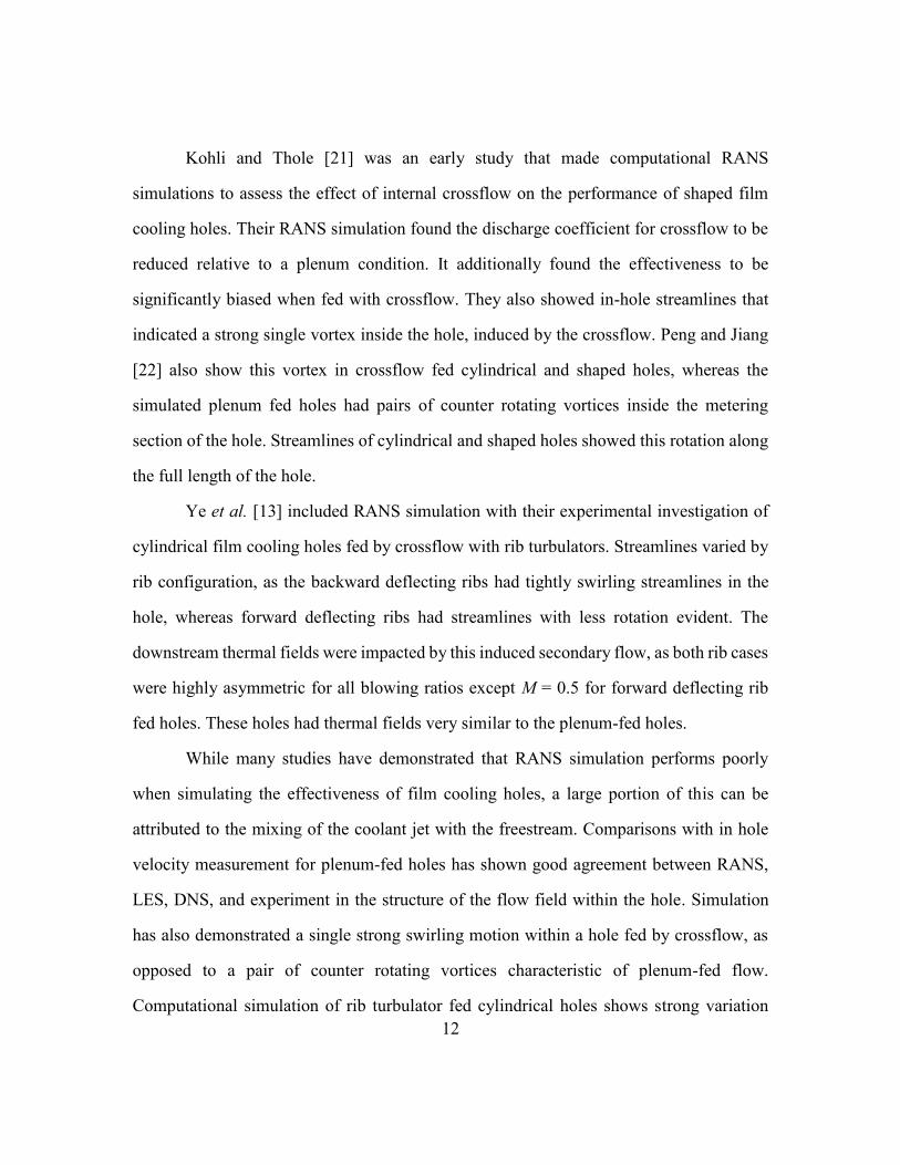
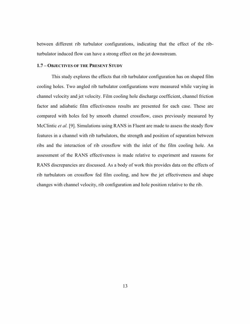
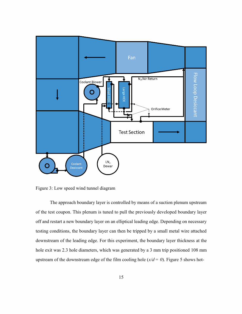
The flat plate facility is a recirculating wind tunnel originally manufactured by

Engineering Laboratory Design and shown in Figure 3. The tunnel test section was

modified by McClintic [23] to add the ability to perform crossflow experiments with a

coolant channel under the test section. Two separate flow systems are necessary for film

cooling: a mainstream loop and a coolant loop.

2.1.1 – Mainstream Flow Loop

The mainstream flow loop is driven by a 30 hp AEROVENT fan. This fan creates

a constant freestream velocity at the desired operating conditions using an ABB VFD. The

flow proceeds through a PID controlled heat exchanger, to set the test section freestream

temperature precisely. Before the test section the mainstream flows through a series of flow

straightening honeycomb and screens, so that that the large scale secondary flows and

eddies generated in the wind tunnel are broken up. The flow is then accelerated to test

section velocity through a nozzle.

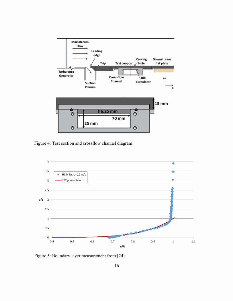
Indicated in Figure 4, the test section has a series of 1 cm diameter vertical bars,

spaced 2.5 cm center-to-center, installed 66 cm upstream of the boundary layer suction

plenum and the test coupon [3]. This generates a high freestream turbulence condition

above the hole consistent with the level of turbulence in the low curvature section of a

turbine guide vane, at Tu = 4.5%. This freestream turbulence had an integral length scale

of Λ𝑥 𝑑⁄ = 2.0 at x/d = 0.

15

The approach boundary layer is controlled by means of a suction plenum upstream

of the test coupon. This plenum is tuned to pull the previously developed boundary layer

off and restart a new boundary layer on an elliptical leading edge. Depending on necessary

testing conditions, the boundary layer can then be tripped by a small metal wire attached

downstream of the leading edge. For this experiment, the boundary layer thickness at the

hole exit was 2.3 hole diameters, which was generated by a 3 mm trip positioned 108 mm

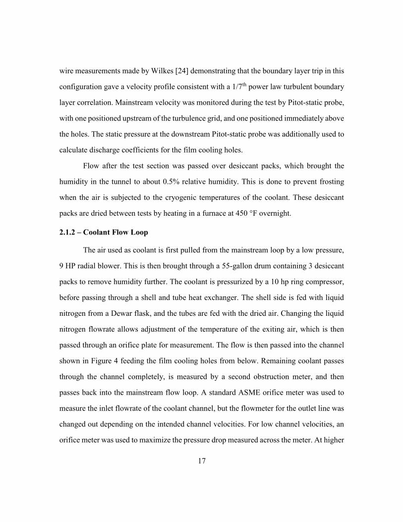
upstream of the downstream edge of the film cooling hole (x/d = 0). Figure 5 shows hot-

Figure 3: Low speed wind tunnel diagram

16

Figure 5: Boundary layer measurement from [24]

Figure 4: Test section and crossflow channel diagram

17

wire measurements made by Wilkes [24] demonstrating that the boundary layer trip in this

configuration gave a velocity profile consistent with a 1/7th power law turbulent boundary

layer correlation. Mainstream velocity was monitored during the test by Pitot-static probe,

with one positioned upstream of the turbulence grid, and one positioned immediately above

the holes. The static pressure at the downstream Pitot-static probe was additionally used to

calculate discharge coefficients for the film cooling holes.

Flow after the test section was passed over desiccant packs, which brought the

humidity in the tunnel to about 0.5% relative humidity. This is done to prevent frosting

when the air is subjected to the cryogenic temperatures of the coolant. These desiccant

packs are dried between tests by heating in a furnace at 450 °F overnight.

2.1.2 – Coolant Flow Loop

The air used as coolant is first pulled from the mainstream loop by a low pressure,

9 HP radial blower. This is then brought through a 55-gallon drum containing 3 desiccant

packs to remove humidity further. The coolant is pressurized by a 10 hp ring compressor,

before passing through a shell and tube heat exchanger. The shell side is fed with liquid

nitrogen from a Dewar flask, and the tubes are fed with the dried air. Changing the liquid

nitrogen flowrate allows adjustment of the temperature of the exiting air, which is then

passed through an orifice plate for measurement. The flow is then passed into the channel

shown in Figure 4 feeding the film cooling holes from below. Remaining coolant passes

through the channel completely, is measured by a second obstruction meter, and then

passes back into the mainstream flow loop. A standard ASME orifice meter was used to

measure the inlet flowrate of the coolant channel, but the flowmeter for the outlet line was

changed out depending on the intended channel velocities. For low channel velocities, an

orifice meter was used to maximize the pressure drop measured across the meter. At higher

18

channel velocity rates, this orifice meter was replaced with a Venturi meter. Total coolant

flow rate was calculated from difference between the channel inlet and exit mass flow rates,

and the coolant jet velocity was calculated assuming equal flow rates through all eight

holes. Tests were repeated with both meters to ensure repeatability between meters. Both

were calibrated against the inlet orifice meter to remove bias error in the ultimate flow rate

calculation.

The density ratio used in this study was DR = 1.2. Typical engine density ratios are

DR ≈ 2.0, however the smooth channel results by McClintic et al. [9] showed very similar

results for DR = 1.2 and DR = 1.8. Consequently, a lower density ratio was used for these

experiments to reduce experimental testing time.

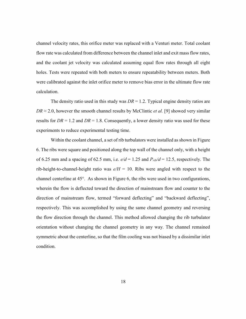
Within the coolant channel, a set of rib turbulators were installed as shown in Figure

6. The ribs were square and positioned along the top wall of the channel only, with a height

of 6.25 mm and a spacing of 62.5 mm, i.e. e/d = 1.25 and Prib/d = 12.5, respectively. The

rib-height-to-channel-height ratio was e/H = 10. Ribs were angled with respect to the

channel centerline at 45°. As shown in Figure 6, the ribs were used in two configurations,

wherein the flow is deflected toward the direction of mainstream flow and counter to the

direction of mainstream flow, termed “forward deflecting” and “backward deflecting”,

respectively. This was accomplished by using the same channel geometry and reversing

the flow direction through the channel. This method allowed changing the rib turbulator

orientation without changing the channel geometry in any way. The channel remained

symmetric about the centerline, so that the film cooling was not biased by a dissimilar inlet

condition.

19

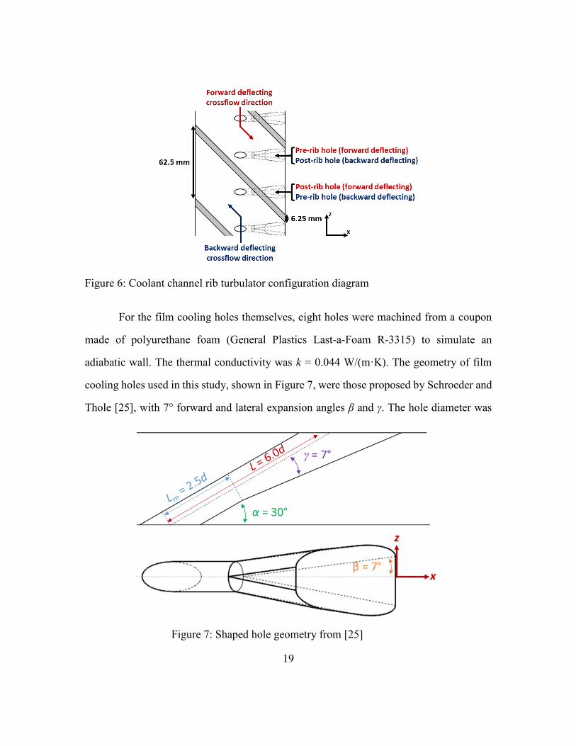
For the film cooling holes themselves, eight holes were machined from a coupon

made of polyurethane foam (General Plastics Last-a-Foam R-3315) to simulate an

adiabatic wall. The thermal conductivity was k = 0.044 W/(m·K). The geometry of film

cooling holes used in this study, shown in Figure 7, were those proposed by Schroeder and

Thole [25], with 7° forward and lateral expansion angles β and γ. The hole diameter was

Figure 7: Shaped hole geometry from [25]

Figure 6: Coolant channel rib turbulator configuration diagram

20

5.0 mm, with a hole-to-hole pitch of P/d = 6.25. This hole diameter was measured by

calipers to be accurate within 0.1 mm. Additionally, the accuracy quoted from the machine

shop is 0.003 in (0.076 mm), so the 0.1 measurement will be taken as more conservative

estimate of the bias uncertainty of the hole diameter.

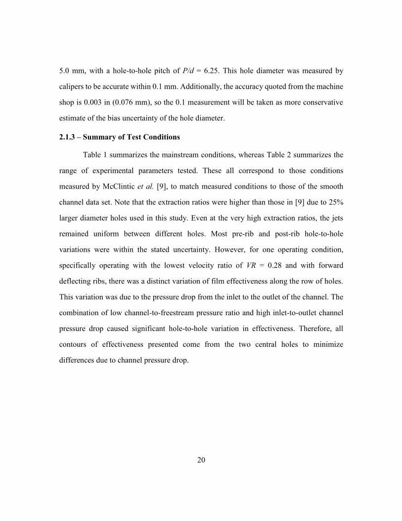
2.1.3 – Summary of Test Conditions

Table 1 summarizes the mainstream conditions, whereas Table 2 summarizes the

range of experimental parameters tested. These all correspond to those conditions

measured by McClintic et al. [9], to match measured conditions to those of the smooth

channel data set. Note that the extraction ratios were higher than those in [9] due to 25%

larger diameter holes used in this study. Even at the very high extraction ratios, the jets

remained uniform between different holes. Most pre-rib and post-rib hole-to-hole

variations were within the stated uncertainty. However, for one operating condition,

specifically operating with the lowest velocity ratio of VR = 0.28 and with forward

deflecting ribs, there was a distinct variation of film effectiveness along the row of holes.

This variation was due to the pressure drop from the inlet to the outlet of the channel. The

combination of low channel-to-freestream pressure ratio and high inlet-to-outlet channel

pressure drop caused significant hole-to-hole variation in effectiveness. Therefore, all

contours of effectiveness presented come from the two central holes to minimize

differences due to channel pressure drop.

21

Table 1: Mainstream operating conditions

Parameter Value Cooling Hole Diameter, d 5.0 mm Mainstream Temp, T

∞ 310 K

Mainstream Velocity, U∞ 24 m/s

Mainstream Turbulence Intensity, Tu 4.5% Turbulence Integral Length Scale, Λ

x/d 2.5

Approach Boundary Layer Thickness, δ/d 3.0 Boundary Layer Displacement Thickness, δ

*/d 0.36

Boundary Layer Momentum Thickness, θ/d 0.27 Boundary Layer Shape Factor, H 1.33 Approach Reynolds Number, Re

d 7,200

Table 2: Crossflow and jet parameters tested

Parameter Value Velocity ratio, 𝑉𝑅 = 𝑈𝑓/𝑈∞ 0.3-1.7 Channel velocity ratio, 𝑉𝑅𝑐 = 𝑈𝑐/𝑈∞ 0.2-0.6 Inlet velocity ratio, 𝑉𝑅𝑖 = 𝑈𝑓/𝑈𝑐 0.5-8.1 Blowing ratio, M 0.3-2.0 Channel inlet Reynolds number, Re

c 14,700-43,000

Extraction ratio, rx 5-72%

2.2 – DATA ACQUISITION AND ANALYSIS

All pointwise measurements were captured with a NI SCXI-1000 Mainframe DAQ

system, with 2 SCXI 1303 temperature modules and 1 SCXI 1301 analog input module for

the pressure transducers. This DAQ used a 12-bit analog to digital converter. The system

was controlled with NI LabVIEW 7.0 software. The temperature and pressure

measurement were averages of 500 individual measurements taken at 200 Hz, over the

course of 2.5 seconds.

2.2.1 – Pressure and Temperature Measurement

Pressure Transducers were used throughout the facility to track static pressure and

calculate mass flowrate. A standard Pitot-static probe was used in the test section to

22

monitor the difference between total and static pressure of the freestream, and thus to

calculate velocity using Bernoulli’s principle:

𝑈∞ = √2∆𝑃

𝜌

For the channel, two pressure transducers were used: one for the static pressure drop from

inlet to outlet, and one to monitor the static pressure relative to atmosphere.

Two pressure transducers were used on each obstruction meter to calculate the mass

flowrate through the coolant line. One transducer monitored the pressure drop across the

obstruction and the other monitored the upstream static pressure relative to atmosphere.

These orifice plates were previously calibrated using a second order curve fit in terms of

orifice meter Reynolds number:

𝐶𝑑 = 𝐴0 + 𝐴1 (106

𝑅𝑒)

34

+ 𝐴2 (106

𝑅𝑒)

32

Where A0, A1, and A2 are the constants of calibration, and Cd is used to calculate mass

flowrate:

�̇� = 𝜌𝜋

4𝑑2

𝐶𝑑

√1 − 𝛽4√

2∆𝑃

𝜌

Where d is the orifice diameter and 𝛽 is the ratio of the orifice throat to inlet diameter.

23

The temperatures were measured using type-E welded junction thermocouples

which were calibrated using the NIST ITS-90 standard calibration for type-E

thermocouples, which has a stated uncertainty of ±1.0K. The freestream and coolant

temperatures were measured simultaneously by thermocouples. Three thermocouples were

averaged for the mainstream temperature and were evenly spread upstream of the leading

edge in Figure 4. The differences between these measurements were primarily due to bias

between thermocouples, on the order of 0.5K This indicates that the measurement

uncertainty would have been substantially improved by manual calibration of the

thermocouples. Two thermocouples measured the channel temperature, one at the inlet and

one at the outlet of the channel. Normally in crossflow measurements, the coolant

temperature rises from the inlet to the outlet due to heating through the walls of the channel.

McClintic [9] showed that using the average channel temperature did not deviate from

direct measurement of the coolant temperature at the entrance of the film cooling hole by

less than ±0.5K. Further, in this study the flow through the channel had to be reversed, so

that both the forward deflecting and backward deflecting rib configurations could be tested.

By alternating feed direction between each measurement VR and VRc, the channel was kept

more evenly cooled, such that the temperature drop across the row of 8 holes was brought

from ∆𝑇~1.1 K in the measurements of McClintic [9] to ∆𝑇~0.66 K on average. This

was predicted from an assumption of a linear temperature variation between the

thermocouples positioned at the inlet and outlet of the channel.

2.2.2 – IR Thermography

A FLIR model A655sc infrared (IR) camera was used to measure the surface

temperature, through a zinc selenide window in the ceiling of the test section. The test

surface was coated with a matte black paint to give uniform emissivity. The camera was

24

calibrated in situ using four thermocouples coupons distributed along the model surface

downstream of the film cooling holes. The thermocouple coupons consisted of type E

surface thermocouples attached to 10 x 10 x 0.5 mm copper coupons. These copper

coupons provided a relatively large area of uniform temperature which facilitated more

accurate calibration of the IR cameras. After calibration these thermocouples coupons were

removed from the surface. The camera viewed the four holes closest to the center of the

test section.

The IR camera views the test section surface at an angle, so a spatial transformation

must be applied to turn the captured surface temperatures from image coordinates to non-

dimensionalized x/d and z/d surface coordinates. This transformation was set by painting

lines on the surface with silver paint, in running in parallel from -10 to 50 x/d. These lines

were positioned so that they were outside the four-hole measurement area, but still visible

by the camera. Tick marks at evenly spaced x/d intervals to provide known surface points.

To calculate the surface transformation, a calibration image is first taken. Loading it into

the FLIR ThermaCAM research software, the pixel coordinates of the marked locations

can be recorded. These are used to create calibration lines that transform pixel coordinates

to surface coordinates. With two surface calibration lines, the whole test area can be

transformed into the appropriate non-dimensionalized coordinates. During actual testing,

multiple calibration images (without film cooling) were taken over the course of the

experiment to ensure that the camera did not move during the test.

Though the foam used was low conductivity, a conduction correction was still

required. A finite element method was used to correct the measured surface temperature to

remove conduction effects for use in the presented adiabatic effectiveness. The test plate

after x/d = 1 was modeled and the measured surface temperature distribution was imposed

as the boundary condition on the surface. A heat transfer coefficient at the surface was

25

imposed, using boundary layer heat transfer correlation (turbulent boundary layer with

adiabatic starting length of the Delrin leading edge), from Incropera and Dewitt [26]. The

heat flux predicted by the FEA was used along with heat transfer coefficient without film

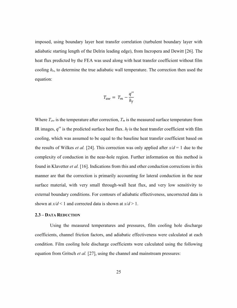
cooling ho, to determine the true adiabatic wall temperature. The correction then used the

equation:

𝑇𝑎𝑤 = 𝑇𝑚 −𝑞′′

ℎ𝑓

Where Taw is the temperature after correction, Tm is the measured surface temperature from

IR images, 𝑞′′ is the predicted surface heat flux. hf is the heat transfer coefficient with film

cooling, which was assumed to be equal to the baseline heat transfer coefficient based on

the results of Wilkes et al. [24]. This correction was only applied after x/d = 1 due to the

complexity of conduction in the near-hole region. Further information on this method is

found in Klavetter et al. [16]. Indications from this and other conduction corrections in this

manner are that the correction is primarily accounting for lateral conduction in the near

surface material, with very small through-wall heat flux, and very low sensitivity to

external boundary conditions. For contours of adiabatic effectiveness, uncorrected data is

shown at x/d < 1 and corrected data is shown at x/d > 1.

2.3 – DATA REDUCTION

Using the measured temperatures and pressures, film cooling hole discharge

coefficients, channel friction factors, and adiabatic effectiveness were calculated at each

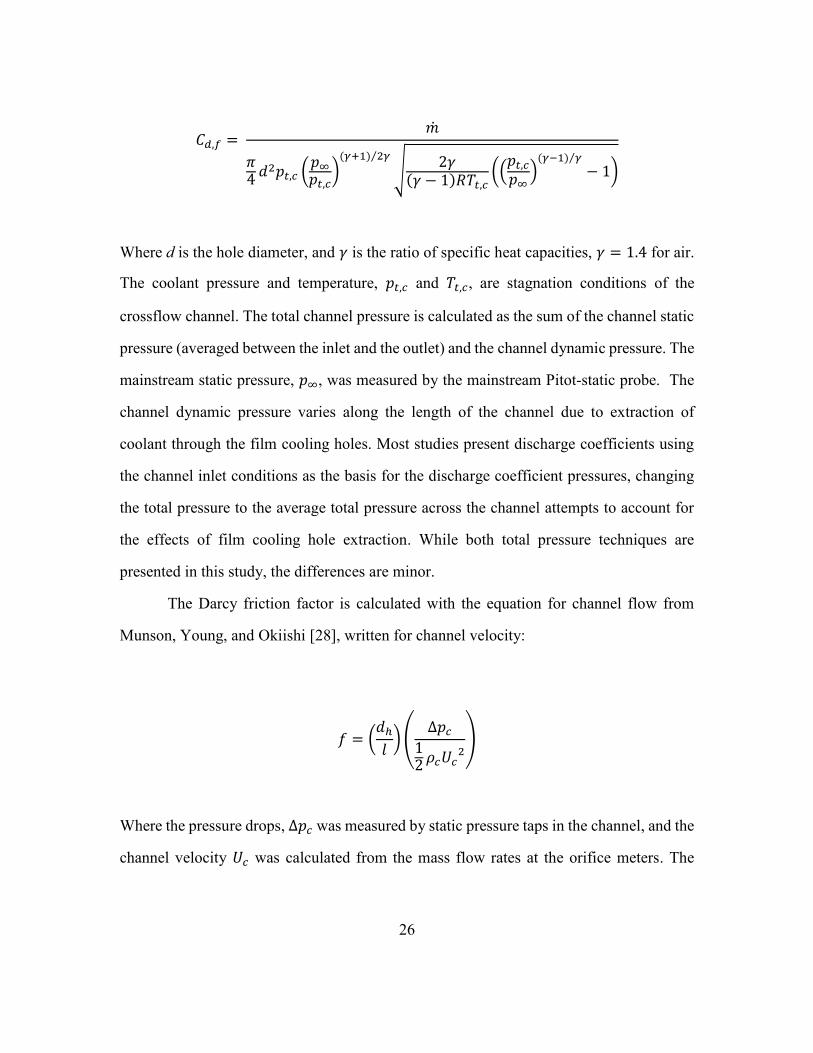
condition. Film cooling hole discharge coefficients were calculated using the following

equation from Gritsch et al. [27], using the channel and mainstream pressures:

26

𝐶𝑑,𝑓 = �̇�

𝜋4 𝑑2𝑝𝑡,𝑐 (

𝑝∞

𝑝𝑡,𝑐)

(𝛾+1) 2𝛾⁄

√2𝛾

(𝛾 − 1)𝑅𝑇𝑡,𝑐((

𝑝𝑡,𝑐

𝑝∞)

(𝛾−1) 𝛾⁄

− 1)

Where d is the hole diameter, and 𝛾 is the ratio of specific heat capacities, 𝛾 = 1.4 for air.

The coolant pressure and temperature, 𝑝𝑡,𝑐 and 𝑇𝑡,𝑐, are stagnation conditions of the

crossflow channel. The total channel pressure is calculated as the sum of the channel static

pressure (averaged between the inlet and the outlet) and the channel dynamic pressure. The

mainstream static pressure, 𝑝∞, was measured by the mainstream Pitot-static probe. The

channel dynamic pressure varies along the length of the channel due to extraction of

coolant through the film cooling holes. Most studies present discharge coefficients using

the channel inlet conditions as the basis for the discharge coefficient pressures, changing

the total pressure to the average total pressure across the channel attempts to account for

the effects of film cooling hole extraction. While both total pressure techniques are

presented in this study, the differences are minor.

The Darcy friction factor is calculated with the equation for channel flow from

Munson, Young, and Okiishi [28], written for channel velocity:

𝑓 = (𝑑ℎ

𝑙) (

∆𝑝𝑐

12 𝜌𝑐𝑈𝑐

2)

Where the pressure drops, ∆𝑝𝑐 was measured by static pressure taps in the channel, and the

channel velocity 𝑈𝑐 was calculated from the mass flow rates at the orifice meters. The

27

channel pressure taps were far enough away from the channel inlet to be measuring fully

developed flow and were symmetric about the center of the test section.

While previous studies [10-12], have used channel inlet velocity to calculate the

Reynolds number and friction factor, the effect of extraction on friction factor and

Reynolds number can be substantial. The Reynolds number changed the most at the highest

extraction ratios. For example, the nominal condition of VR = 1.38 and VRc =0.2 had an

extraction ratio of 61%. This caused a Rec,in = 14,900 to decrease to a Rec,avg = 10,300. In

this study, friction factors and Reynolds numbers calculated from inlet channel velocity

and average channel velocity are presented for comparison. They are indicated as fin and

favg, respectively. This study found that the friction factor scaled better with Reynolds

number when both were based on the average of the channel inlet and outlet velocities,

discussed in more detail in Chapter 5.

Adiabatic effectiveness was calculated for the surface from the calibrated,

conduction corrected IR images. For each experimental set point, 5 images were taken and

averaged together. Random variation between images was one component of precision

uncertainty, in addition to in-test and test-to-test repeatability. The adjusted surface

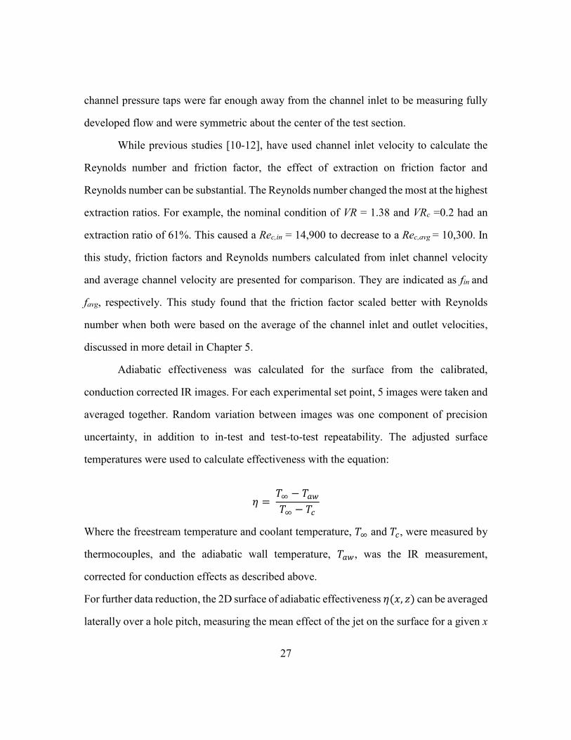
temperatures were used to calculate effectiveness with the equation:

𝜂 = 𝑇∞ − 𝑇𝑎𝑤

𝑇∞ − 𝑇𝑐

Where the freestream temperature and coolant temperature, 𝑇∞ and 𝑇𝑐, were measured by

thermocouples, and the adiabatic wall temperature, 𝑇𝑎𝑤, was the IR measurement,

corrected for conduction effects as described above.

For further data reduction, the 2D surface of adiabatic effectiveness 𝜂(𝑥, 𝑧) can be averaged

laterally over a hole pitch, measuring the mean effect of the jet on the surface for a given x

28

location. This is the laterally-averaged effectiveness, �̅�(𝑥). It can further be averaged to

find the contribution to the surface at once condition, spatially-averaged effectiveness, �̿�.

2.4 – UNCERTAINTY ANALYSIS

Overall uncertainty of the experimental measurements comes from two

components: bias and precision. The bias uncertainty is due to uncertainty in instrument

calibration and correction techniques, which both result in an uncertainty in the final

measured parameter due to the imperfect nature of the correction process. The precision

uncertainty is due to random variation of the measurement variables over the course of

testing. Reported uncertainties were estimated using the method of sequential perturbation,

as described by Moffat et al. [29]. This method calculates a contribution of the uncertainty

in a calculated parameter due to the uncertainty in an input measurement. The measured

value is perturbed by the uncertainty (bias or precision) of the measurement method, and

then the calculation of the final parameter is carried forward with this perturbed value. The

difference between the perturbed parameter value and the actual parameter value is the

contribution to the bias or precision uncertainty due to the uncertainty in the measured

value. This process is then sequentially performed for all measured values and their

associated uncertainties. The root-sum squared of all propagated uncertainty give the

combination of all measurement uncertainties in the overall bias or precision uncertainty

for that parameter.

2.4.1 – Precision Uncertainty and Repeatability

The precision uncertainty is in part due to the random fluctuation within a given set

of measurements, on timescales ranging from the electronic noise of the measurement

device to daily barometric pressure fluctuations and longer. The relatively short timescale

precision uncertainty can be quantified by averaging multiple measurements together over

29

the course of a single measurement. The electronic noise precision is captured for the single

point measurements (thermocouples and pressure transducers) by averaging 500

measurements taken over the course of 2.5 seconds. This variation is a negligible

contribution to the total precision uncertainty of those measurements for this experiment.

Moderate timescale variation is quantified in this experiment by taking five sequential

measurements (spaced approximately 1 minute apart) and averaged, and the corresponding

uncertainty for n = 5 is calculated, taking adiabatic effectiveness as an example:

𝛿(𝜂)𝑝 = 𝑡95

𝜎𝜂

√𝑛

The uncertainty due to in-measurement random variation for the pointwise

measurements is calculated in the same manner and were taken at the same time as the IR

images. The longer timescales of precision uncertainty are more difficult to quantify, as

they can include systematic but unknown variance in the conditions of the experiment as

well as random variation.

Repeatability is a measure of the variation of a measurement due to longer timescale

fluctuations of measurement, and systematic but variable drift in the setpoint. The

repeatability was determined for all experimentally measured values at the beginning and

end of each test, and across two separated days of testing. The same set point was repeated

both in-test with the orifice plate at the beginning and end of the first day (~8 hours apart)

and test-to-test with the Venturi meter on the second day of testing. The repeat set point

was VRc = 0.3 and VR = 1.11 for both forward and backward deflecting ribs. Figure 8 shows

repeat cases in terms of the laterally averaged effectiveness. From the figure, it seems that

the repeat tests were lower than the initial baseline test for the forward deflecting rib

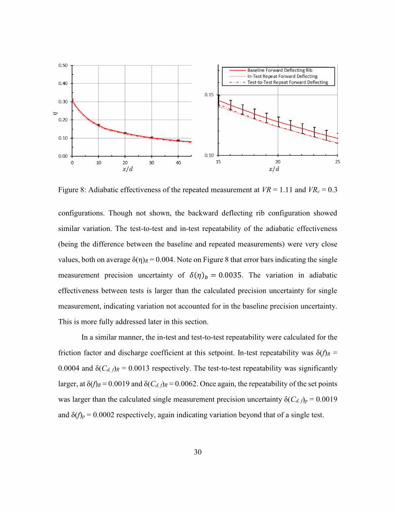
30

configurations. Though not shown, the backward deflecting rib configuration showed

similar variation. The test-to-test and in-test repeatability of the adiabatic effectiveness

(being the difference between the baseline and repeated measurements) were very close

values, both on average δ(η)R = 0.004. Note on Figure 8 that error bars indicating the single

measurement precision uncertainty of 𝛿(𝜂)𝑏 = 0.0035. The variation in adiabatic

effectiveness between tests is larger than the calculated precision uncertainty for single

measurement, indicating variation not accounted for in the baseline precision uncertainty.

This is more fully addressed later in this section.

In a similar manner, the in-test and test-to-test repeatability were calculated for the

friction factor and discharge coefficient at this setpoint. In-test repeatability was δ(f)R =

0.0004 and δ(Cd, f)R = 0.0013 respectively. The test-to-test repeatability was significantly

larger, at δ(f)R = 0.0019 and δ(Cd, f)R = 0.0062. Once again, the repeatability of the set points

was larger than the calculated single measurement precision uncertainty δ(Cd, f)p = 0.0019

and δ(f)p = 0.0002 respectively, again indicating variation beyond that of a single test.

Figure 8: Adiabatic effectiveness of the repeated measurement at VR = 1.11 and VRc = 0.3

31

The contribution to uncertainty from the repeatability is non-negligible and is

primarily due to the window of accepted operating ranges for a given setpoint (δVR =

±0.04, δDR = ±0.025, and δVRcR = ±0.006). Therefore, tests of the same nominal setpoint

can be considered the same condition, despite repeatability of the flow parameters greater

than the uncertainty. When scaling the behavior of the holes with VR, VRc, and DR, all

measurements were scale with the measured flow parameters (rather than the nominal

conditions) to take this small variation into account. In future tests, these flow rate ranges

should be further narrowed to minimize the uncertainty in measured parameters due to

repeatability between tests.

2.4.2 – Flowrate Uncertainty

The flow rate measurements were made by obstruction meters (for the coolant) and

Pitot-static probe (for the mainstream). Consequently, the bias uncertainty in VR and VRc

are a result of the fossilized biases in the resulting from calibration of the obstruction meters

pressure transducers, thermocouples, and geometry. New calibrations of the instruments

used in the small wind tunnel were not performed for this study, meaning that the system

calibrations are from the data of Anderson [3] and McClintic [9], who have calibrated the

instruments most recently.

The bias uncertainty of the velocity ratio was primarily influenced uncertainty of

the hole diameter and the pressure transducer bias for channel inlet orifice meter and varied

for different blowing ratios. For most conditions it a combined bias uncertainty of

𝛿(𝑉𝑅)𝑏 = 4.5% on average. For the repeated point VR = 1.11, VRc = 0.3 it was 𝛿(𝑉𝑅)𝑏 =

0.046. The bias decreased with decreasing blowing ratio, however at the VR = 0.28

measurements (due to relatively small mass flow rates) the relative uncertainty was as high

32

as 𝛿(𝑉𝑅)𝑏 = 10%, for an absolute uncertainty of 𝛿(𝑉𝑅)𝑏 = 0.028. The precision

uncertainty for the measurements was typically at 𝛿(𝑉𝑅)𝑝 = 0.0038 for all conditions, with

no systematic variation of uncertainty between different VR. Since the bias uncertainty is

much larger than the precision, the overall uncertainty for a typical measurement was

around 𝛿𝑉𝑅 = 4.6%, up to a maximum of 10.5% at the lowest VR.

For the channel velocity ratio, the bias uncertainty was primarily due to the

uncertainty of the pressure transducers used to measure the orifice meter ∆𝑃 and the coolant

temperature thermocouple. The overall bias uncertainty had a typical value of 𝛿(𝑉𝑅𝑐)𝑏 =

0.0025, which as a relative uncertainty varied between 𝛿(𝑉𝑅𝑐)𝑏 = 0.5 − 1.0%. For these

measurements, the precision uncertainty was around 𝛿(𝑉𝑅𝑐)𝑝 = 0.00065, such that the

overall uncertainty was again dominated by the bias uncertainty. The overall relative

uncertainty 𝛿𝑉𝑅𝑐 was therefore between 0.55-1.05%.

The density ratio bias uncertainty was almost completely a function of the

thermocouple bias. It was nearly constant at 𝛿(𝐷𝑅)𝑏 = 0.0060, or 0.5%. The precision

uncertainty was an order of magnitude lower, 𝛿(𝐷𝑅)𝑝 = 0.00044, so the overall

uncertainty of the density ratio is of 𝛿𝐷𝑅 = 0.0061.

2.4.3 – Discharge Coefficient Uncertainty

The discharge coefficient involved measurements by pressure transducers on the

channel, in addition to the mass flow rates measured from the orifice meters. For most set

points, the bias uncertainty was driven by the uncertainty in the hole diameter, but at the

lowest velocity ratios, the uncertainty in mass flow rate due to uncertainty in the pressure

33

transducer across the inlet orifice meter became the dominant contribution. Thus, for most

conditions, the discharge coefficient had an absolute bias uncertainty of around δ(Cd, f)b =

0.033 or relative uncertainty δ(Cd, f)b = 4.1-5.9%, but for the lowest velocity ratio

measurements, the relative uncertainty was closer to 10%, due to both higher uncertainty

and smaller values of the discharge coefficient in these cases. The precision uncertainty of

the discharge coefficient was on average 𝛿(𝐶𝑑,𝑓)𝑝

= 0.0019 from single test random

variation and 𝛿(𝐶𝑑,𝑓)𝑝

= 0.0064 with long timescale variation due to flow rate considered.

This means the overall discharge coefficient uncertainty was 𝛿𝐶𝑑,𝑓 = 0.034 for a typical

measurement.

2.4.4 – Friction Factor Uncertainty

The friction factor uncertainty is only dependent on the uncertainty of the pressure

transducer measuring the pressure drop across the channel, and the uncertainties of mass

flowrates from the obstruction meters. Since the pressure drops were so small across the

channel, the uncertainty from the transducer were the main contribution, rather than the

uncertainty in mass flowrate through the channel. The bias uncertainty was larger at lower

channel velocity ratio, ranging from 𝛿(𝑓)𝑏 = 0.0025 at VRc = 0.2 to 𝛿(𝑓)𝑏 = 0.0007 at

VRc = 0.6. This meant relative bias uncertainties ranged from 𝛿(𝑓)𝑏 = 0.5 − 2.7%, on

average 1.2%. The precision uncertainty was on the order of the bias, around 𝛿(𝑓)𝑝 =

0.0002 from single test fluctuations alone but 𝛿(𝑓)𝑝 = 0.0019 due to the variation of flow

rate variation between tests. This did contribute to a higher overall uncertainty at the higher

channel velocity flow rates, such that the average relative overall uncertainty was 𝛿𝑓 =

2.32%

34

2.4.5– Adiabatic Effectiveness Uncertainty

The uncertainty of the effectiveness measurement is influenced by the calibration

of the IR camera, as well as the uncertainties due to assumptions in the finite element

modelling for conduction correction. Based on the work of Klavetter et al. [16], the effect

of the conduction correction was smaller than the uncertainty due to camera calibration for

measurements downstream, which is why the spatially averaged effectiveness is averaged

from 5 < x/d < 25. The combined bias uncertainty was 𝛿(𝜂)𝑏 = 0.017 on average, with

due primarily to the bias of the thermocouples used for freestream and coolant temperature.

The corresponding precision uncertainty was at most 𝛿(𝜂)𝑝 = 0.0053. The two primary

contributions (with about equal magnitude) were the fluctuation of the IR camera

temperature readings within a measurement and the variation due to flowrate uncertainty,

which is discussed in more detail in the next section. This lead to an overall uncertainty in

adiabatic effectiveness of 𝛿𝜂 = 0.018.

35

Chapter 3: Computational Methods

A RANS simulation with a realizable 𝑘 − 휀 turbulence model and enhanced wall

treatment was used to simulate a pair of film cooling holes fed by a crossflow channel with

rib turbulators. Simulations were performed in ANSYS Fluent. These tests were done to

evaluate the ability of simulation to predict film cooling effectiveness, and to better

understand the complex flow field around the film cooling hole.

3.1 – RANS SIMULATION METHOD

As opposed to the time resolved numerical simulations of turbulence, such as direct

numerical simulation (DNS) and large eddy simulation (LES), Reynolds-Averaged Navier-

Stokes (RANS) simulation predicts a time-averaged flow field. Beginning from the Navier-

Stokes equations for continuity and momentum:

𝜕𝑈𝑖

𝜕𝑥𝑖= 0

𝜕𝑈𝑖

𝜕𝑡+

𝜕

𝜕𝑥𝑗(𝑈𝑖𝑈𝑗) = −

1

𝜌

𝜕𝑃

𝜕𝑥𝑖+ 𝜈

𝜕2𝑈𝑖

𝜕𝑥𝑗𝜕𝑥𝑗

In Einstein’s summation notation, where repeated indices imply summation. These assume

a Newtonian, constant property, incompressible fluid. The Reynolds averaging process

decomposes the velocity and pressure field into the combination of mean and fluctuating

components, 𝑈𝑖 = 𝑈�̅� + 𝑢𝑖′. This changes the momentum equation:

𝜕

𝜕𝑥𝑗(𝑈�̅�𝑈�̅�) = −

1

𝜌

𝜕�̅�

𝜕𝑥𝑖−

𝜕𝑢𝑖′𝑢𝑗

′̅̅ ̅̅ ̅̅

𝜕𝑥𝑗+ 𝜈

𝜕2𝑈�̅�

𝜕𝑥𝑗𝜕𝑥𝑗

36

This equation forms the basis of RANS simulation. The turbulent fluctuating

velocity contributes as the 𝑢𝑖′𝑢𝑗

′̅̅ ̅̅ ̅̅ term, which is commonly called the Reynolds stress.

Determining what this stress is for a given point in a flow field it the central difficulty

behind RANS modelling.

3.1.1 – Turbulence Closure

The problem of determining the Reynolds stress is commonly referred to as the

“turbulence closure” problem. Many models have been proposed over the years, with

varying degrees of accuracy. Most commonly used are the linear eddy viscosity models,

which assume via the Boussinesq hypothesis that the Reynolds stress is linear in the mean

strain rate, with turbulent (or eddy) viscosity, 𝑣𝑇:

𝑢𝑖′𝑢𝑗

′̅̅ ̅̅ ̅̅ = 𝑣𝑇 (𝜕𝑈�̅�

𝜕𝑥𝑗+

𝜕𝑈�̅�

𝜕𝑥𝑖) −

2

3𝑘𝛿𝑖𝑗 = 2𝑣𝑇𝑆𝑖𝑗 −

2

3𝑘𝛿𝑖𝑗

𝑆𝑖𝑗 is called the mean strain rate tensor and appears frequently in the 𝑘 − 휀 model.

This hypothesis implicitly assumes the Reynolds stress to be isotropic, which has been

shown to be not true in many experimental measurements of turbulent shear flow. Higher

complexity models track the individual components of the Reynolds stress tensor directly,

but greatly increase complexity of computation.

The 𝑘 − 휀 model computes turbulent viscosity by tracking the transport of two

turbulent parameters through the fluid: 𝑘, the kinetic energy associated with local turbulent

fluctuations, and 휀, the specific dissipation rate of turbulent kinetic energy. This is done by

formulating transport equations like the momentum equation for these scalar variables [30]:

𝜕

𝜕𝑥𝑗(𝑘𝑈�̅�) = −

𝜕

𝜕𝑥𝑗[(𝑣 +

𝑣𝑇

𝜎𝑘)

𝜕𝑘

𝜕𝑥𝑗] + 2𝜈𝑇𝑆𝑖𝑗𝑆𝑖𝑗 − 휀

37

𝜕

𝜕𝑥𝑗(휀𝑈�̅�) = −

𝜕

𝜕𝑥𝑗[(𝑣 +

𝑣𝑇

𝜎𝜀)

𝜕휀

𝜕𝑥𝑗] + 2𝐶1𝑆𝑖𝑗𝑆𝑖𝑗 − 2𝐶2

휀2

𝑘 + √𝑣휀

The kinetic energy equation is an analytic representation of the transportation and

production of turbulent kinetic energy. However, the dissipation is semi-empirical. The

form of last two terms on the right-hand side- which are the source and sink of dissipation-

are chosen to make the simulation match more closely to experimental data. 𝜎𝑘 and 𝜎𝜀 are

the turbulent Prandtl numbers of 𝑘 and 휀, and are chosen to more closely match experiment.

Once 𝑘 and 휀 have been determined, the turbulent viscosity can be calculated from:

𝑣𝑇 = 𝐶𝜇

𝑘2

휀

In the standard 𝑘 − 휀 model, 𝐶𝜇is a constant. However, with the realizable 𝑘 − 휀

model implemented in Fluent, it varies depending on the local mean strain rate, rotation

rate, angular velocity, 𝑘 and 휀. This again is done to match with experimental results more

closely and preserves vector identities of the Reynolds stresses that are not guaranteed by

the standard model [31].

The improvements by the realizable 𝑘 − 휀 by the above adjustments result in better

simulation of regions of strong curvature, and flows with vortices, rotation and separation.

However, two major drawbacks are still apparent. 𝑘 − 휀 applies to only turbulent driven

flows, meaning that inside the viscous sublayer of a turbulent boundary layer, the model is

invalid, necessitating the use of near-wall treatment separate from the overall model.

Second, the actual anisotropy of real Reynolds stress leads to inaccuracies in mixing flows

which cannot be addressed by further extensions to the same model.

38

3.1.2 – Wall Functions

Fluent has several methods to treat wall bounded flows. The chosen method for this

set of simulations was so-called “Enhanced Wall Treatment”, which seeks to ensure the

accurate capture of a boundary layer when the simulating mesh is fine enough to resolve

the viscous sublayer, but still has reasonable accuracy if the grid is not quite high enough

resolution.

In the standard two-layer model, well resolved meshes have grids fine enough to

have multiple cells within the viscous sublayer, with a typical first-cell 𝑦+ ≈ 1. The

software then splits the domain into regions of viscous-dominated flow and fully-turbulent,

determined by the cell’s distance from the nearest wall. The cutoff between the two is a

Rey of 200, where Rey is defined as:

𝑅𝑒𝑦 =𝑦√𝑘

𝜐

In the turbulent region, the 𝑘 − 휀 model is used as normal. In the viscous region, a

different, one variable model [32] is used. There the turbulent viscosity is calculated not

from 𝑘 and 휀, but just from k:

𝑣𝑇 = 𝐶𝜇ℓ𝜇√𝑘

ℓ𝜇 = 𝑦𝐶ℓ∗(1 − 𝑒−𝑅𝑒𝑦/𝐴𝜇)

With 𝐶ℓ∗ and 𝐴𝜇 being constants. In the enhanced wall treatment method, this

algebraic determination is then blended to match exactly the 𝑘 − 휀 formulation outside the

viscous model. This extra step aids in the solution convergence when the outer layer is does

not match the predictions from the inner layer.

39

For the film cooling simulation, all meshes were of sufficient resolution (checked

after convergence) such that the 𝑦+ ≈ 1 condition for the first cell above the wall was

satisfied.

3.1.3 – Thermal Transport

Transport in Fluent is modeled with a scalar transport equation for internal energy

E similar in form to those above for 𝑘 and 휀:

𝜕

𝜕𝑥𝑗(𝐸𝑈�̅�) = −

𝜕

𝜕𝑥𝑗(𝑘𝑒𝑓𝑓

𝜕𝑇

𝜕𝑥𝑗) + �̇�

Where the thermal conductivity of the medium, k, is modified by the local turbulent

viscosity, 𝜇𝑇 = 𝜌𝜐𝑇:

𝑘𝑒𝑓𝑓 = 𝑘 +𝑐𝑝𝜇𝑇

𝑃𝑟𝑇

For Fluent, the turbulent Prandtl number, 𝑃𝑟𝑇, is a constant. This constant turbulent

Prandtl number and the underlying assumption – that internal energy is transported in the

direction of the mean temperature gradient – form a common scalar transport assumption,

the gradient diffusion hypothesis. It’s well known that this is not an excellent assumption

for many turbulent mixing phenomena. In particular, [20] has shown through the

simulation of a film cooling hole using LES that the thermal diffusion can occur nearly

perpendicular to the mean temperature gradient when mixing the jet with the freestream.

Hence this model is one of the biggest contributors to the inaccuracy of film cooling

simulations in RANS and will continue to affect results in this study.

3.3 – BOUNDARY CONDITIONS AND ADJUNCT SIMULATIONS

For the film cooling hole simulations, three views of the primary domain are shown

in Figure 9. The geometry consisted of two shaped film cooling holes with the same

dimensions as those in the experiment. A slice of freestream was included 20 diameters

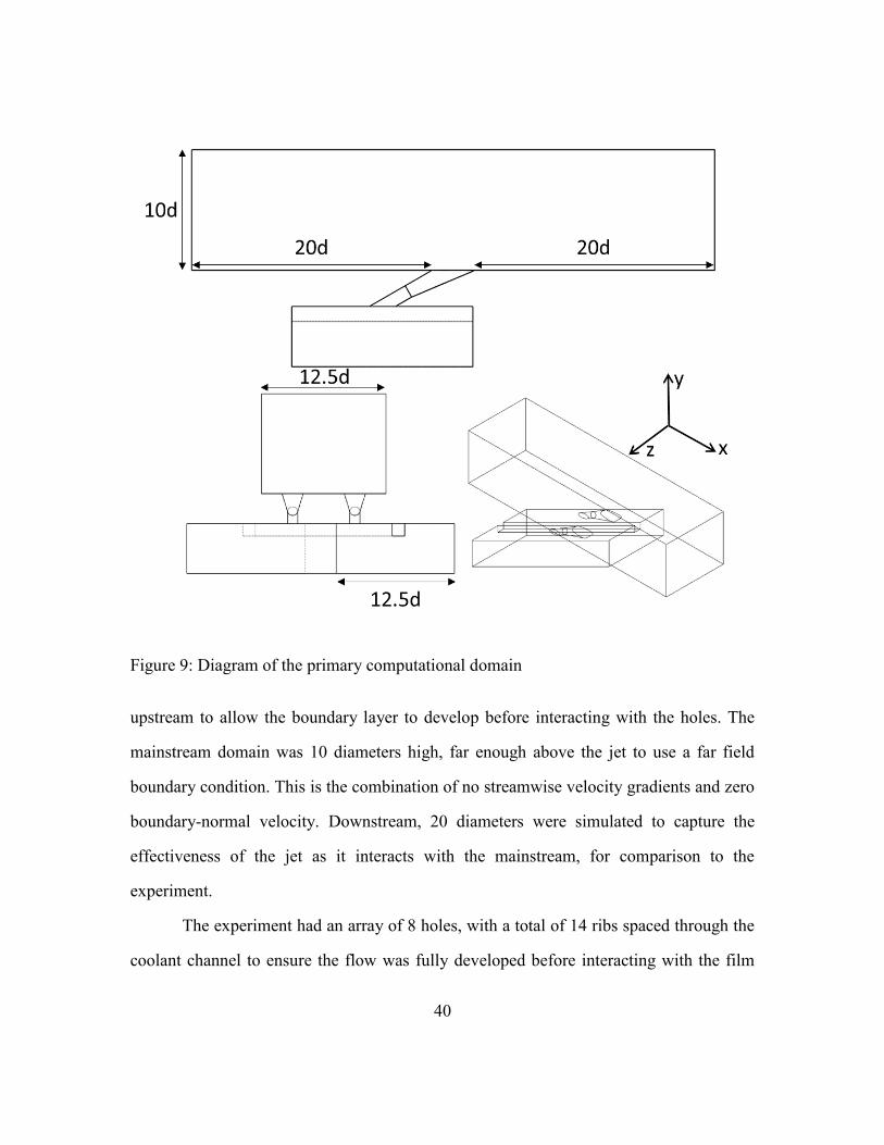
40

upstream to allow the boundary layer to develop before interacting with the holes. The

mainstream domain was 10 diameters high, far enough above the jet to use a far field

boundary condition. This is the combination of no streamwise velocity gradients and zero

boundary-normal velocity. Downstream, 20 diameters were simulated to capture the

effectiveness of the jet as it interacts with the mainstream, for comparison to the

experiment.

The experiment had an array of 8 holes, with a total of 14 ribs spaced through the

coolant channel to ensure the flow was fully developed before interacting with the film

Figure 9: Diagram of the primary computational domain

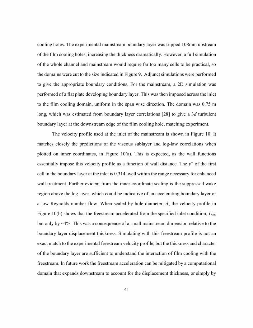
41

cooling holes. The experimental mainstream boundary layer was tripped 108mm upstream

of the film cooling holes, increasing the thickness dramatically. However, a full simulation

of the whole channel and mainstream would require far too many cells to be practical, so

the domains were cut to the size indicated in Figure 9. Adjunct simulations were performed

to give the appropriate boundary conditions. For the mainstream, a 2D simulation was

performed of a flat plate developing boundary layer. This was then imposed across the inlet

to the film cooling domain, uniform in the span wise direction. The domain was 0.75 m

long, which was estimated from boundary layer correlations [28] to give a 3d turbulent

boundary layer at the downstream edge of the film cooling hole, matching experiment.

The velocity profile used at the inlet of the mainstream is shown in Figure 10. It

matches closely the predictions of the viscous sublayer and log-law correlations when

plotted on inner coordinates, in Figure 10(a). This is expected, as the wall functions

essentially impose this velocity profile as a function of wall distance. The y+ of the first

cell in the boundary layer at the inlet is 0.314, well within the range necessary for enhanced

wall treatment. Further evident from the inner coordinate scaling is the suppressed wake

region above the log layer, which could be indicative of an accelerating boundary layer or

a low Reynolds number flow. When scaled by hole diameter, 𝑑, the velocity profile in

Figure 10(b) shows that the freestream accelerated from the specified inlet condition, Uin,

but only by ~4%. This was a consequence of a small mainstream dimension relative to the

boundary layer displacement thickness. Simulating with this freestream profile is not an

exact match to the experimental freestream velocity profile, but the thickness and character

of the boundary layer are sufficient to understand the interaction of film cooling with the

freestream. In future work the freestream acceleration can be mitigated by a computational

domain that expands downstream to account for the displacement thickness, or simply by

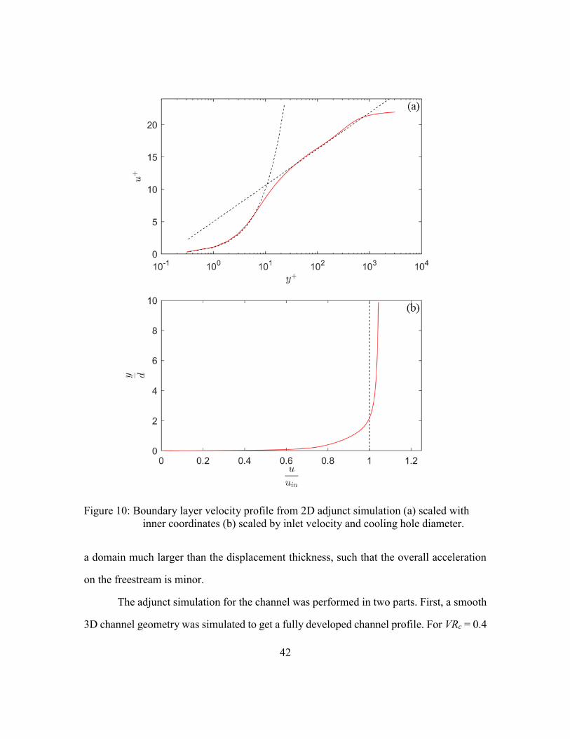
42

a domain much larger than the displacement thickness, such that the overall acceleration

on the freestream is minor.

The adjunct simulation for the channel was performed in two parts. First, a smooth

3D channel geometry was simulated to get a fully developed channel profile. For VRc = 0.4

Figure 10: Boundary layer velocity profile from 2D adjunct simulation (a) scaled with

inner coordinates (b) scaled by inlet velocity and cooling hole diameter.

43

this corresponds to a 9.6 m/s mean velocity at the inlet of the channel. This fully developed

profile was then fed into the geometry in Figure 11, simulating a 9-rib channel

configuration. Once the simulation was run to convergence, a velocity and turbulent kinetic

energy profile between ribs was taken to be used for the channel in the film cooling

simulation. These profiles are shown for both the first smooth channel simulation and then

the subsequent rib-turbulated channel simulation in Figure 12. The coordinates are

normalized by the film cooling hole diameter. Though the rib turbulated channel profile is

a plane at a 45° angle to the channel centerline, the profile viewed from the positive z-

direction has the same dimensions as the smooth channel cross section. The smooth

channel mean velocity is relatively uniform spanwise for the middle 80% of the channel,

as would be expected in this high aspect ratio channel flow. In contrast, the mean velocity

of the rib tubulated channel shows significant variation, indicative of the highly mixing rib

Figure 11: Rib turbulated channel geometry for the adjunct simulation

44

turbulated flow. Additionally, the turbulent kinetic energy for the rib turbulated channel is

non-homogenous and much higher than the smooth channel, another expected effect of the

rib turbulators. With the rib turbulated channel profile applied to the inlet of the film

cooling simulation, the conditions for simulating the film cooling fed by this channel are

appropriately modeled.

The mid-plane between ribs was chosen as the inlet boundary so that the boundary

would not intersect a rib and complicate the simulation geometry. Film cooling simulations

failed when first attempted with the channel inlet and outlet intersecting ribs, as the

software had difficulty with the complex mesh near the intersection. The adjunct simulation

process was repeated with the same conditions but feeding the channel from the opposite

direction. This resulted in the backward deflecting rib turbulator boundary condition.

For the full film cooling hole simulation, both adjunct simulation velocity boundary

conditions were applied to the inlet of the mainstream and channel. Similarly, profiles of k

and 휀 were used from the same simulations. The freestream and channel temperature were

set to match the experiment, 310 and 254 K directly. The mainstream outlet was set as a

pressure outlet, specifying atmospheric pressure at the outlet. Control over the variation of

Figure 12: Velocity and turbulent kinetic energy contours for the channel adjunct

simulations

45

blowing ratio was achieved by varying the outlet pressure of the channel. Increasing the

channel pressure correspondingly increases the velocity ratio. The channel outlet pressure

was set using the experimentally measured discharge coefficients to estimate the required

pressure ratio. However, the simulation required a different than predicted pressure to

achieve the desired VR, so channel pressure boundary conditions were iterated manually

until the mass flowrate through the holes was correct.

3.4 – GRID GENERATION

An appropriate grid is key to finding numerical solutions in RANS. Already

mentioned was dependence on fine resolution near walls, so that the enhanced wall

treatment can be used for the 𝑘 − 휀 model. Additionally, solution convergence can be

sensitive to the cell skewness and the cell Courant number, defined as:

𝐶 = uΔ𝑡

Δ𝑥

Where the local velocity, u, is compared with the characteristic length of the cell and the

RANS “pseudo-time step”. This pseudo-timestep is a parameter adjustable in fluent to aid

in stability. However, decreasing this timestep at each iteration leads to longer required

simulation time, so a balance between mesh resolution and timestep requirements must be

sought for quick and accurate solution convergence.

Mesh generation is itself a large field, but there are two broad categories of mesh

types: structured and unstructured. Unstructured meshes fill the domain with cells using

some general space-filling algorithm, generating a mesh that is non-uniform but generally

adapts to geometry and expected flow physics. A structured mesh breaks the domain into

simplified regions, meshes those regions, and then recombines the meshes into a singular

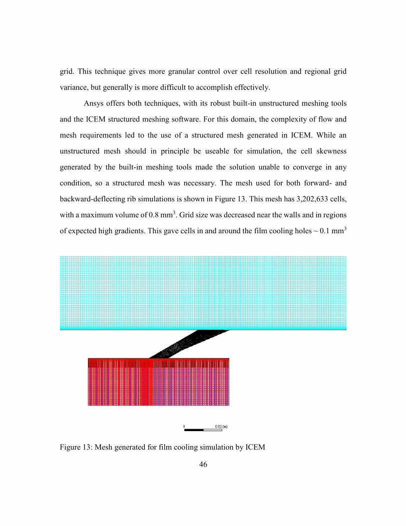
46

grid. This technique gives more granular control over cell resolution and regional grid

variance, but generally is more difficult to accomplish effectively.

Ansys offers both techniques, with its robust built-in unstructured meshing tools

and the ICEM structured meshing software. For this domain, the complexity of flow and

mesh requirements led to the use of a structured mesh generated in ICEM. While an

unstructured mesh should in principle be useable for simulation, the cell skewness

generated by the built-in meshing tools made the solution unable to converge in any

condition, so a structured mesh was necessary. The mesh used for both forward- and

backward-deflecting rib simulations is shown in Figure 13. This mesh has 3,202,633 cells,

with a maximum volume of 0.8 mm3. Grid size was decreased near the walls and in regions

of expected high gradients. This gave cells in and around the film cooling holes ~ 0.1 mm3

Figure 13: Mesh generated for film cooling simulation by ICEM

47

volume on average and further increased resolution at the walls of the film cooling hole, to

a first cell height of 0.01mm.

A rigorous method of determining whether a grid is sufficient for resolving a given

flow field is to perform a grid independence study. In this test, multiple grids of varying

resolution are used to simulate the same conditions, monitoring a parameter of interest

related to the flow field. As the grid resolution increases, it would be expected that the

parameter would converge to a single value, indicating that changing the grid further would

not result in increased accuracy or a change to the solution. While a grid independence

study was not performed for this exact study, similar simulations done by Jones [33]

indicate that the simulation of film cooling holes fed by crossflow are insensitive to

increased grid resolution beyond a total of ~10 cells across the width of the hole when done

with the simulation methods in Fluent described above. Since the resolution in the film

cooling holes of this mesh give much more than 30 cells across the hole, this is expected

to be sufficient resolution for the solution to be independent of the grid.

3.5 – CONVERGENCE CRITERIA

RANS simulation in Fluent finds a solution to discretized versions of the RANS

equations via iterating toward a solution using a pseudo-time step, improving the numerical

solution from one iteration to the next. To track the stability of the solution and achieve a

measure of uncertainty in computation, the residual can be tracked through the iterations.

A residual is the sum of the imbalances of a solution variable over the whole domain. For

example, the mass residual is the sum of the mass “created” in each cell by inaccuracy due

to truncation and round-off error. As the solution stabilizes, the residuals decrease until

either the maximum number of iterations is reached, or a minimum threshold value of

residuals is attained.

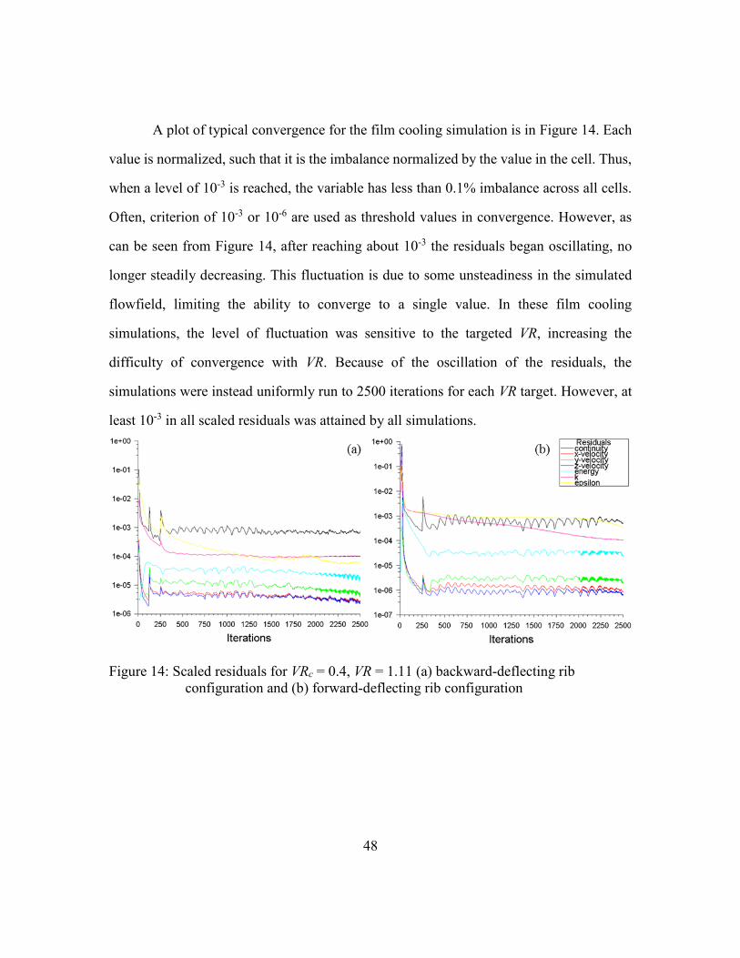
48

A plot of typical convergence for the film cooling simulation is in Figure 14. Each

value is normalized, such that it is the imbalance normalized by the value in the cell. Thus,

when a level of 10-3 is reached, the variable has less than 0.1% imbalance across all cells.

Often, criterion of 10-3 or 10-6 are used as threshold values in convergence. However, as

can be seen from Figure 14, after reaching about 10-3 the residuals began oscillating, no

longer steadily decreasing. This fluctuation is due to some unsteadiness in the simulated

flowfield, limiting the ability to converge to a single value. In these film cooling

simulations, the level of fluctuation was sensitive to the targeted VR, increasing the

difficulty of convergence with VR. Because of the oscillation of the residuals, the

simulations were instead uniformly run to 2500 iterations for each VR target. However, at

least 10-3 in all scaled residuals was attained by all simulations.

Figure 14: Scaled residuals for VRc = 0.4, VR = 1.11 (a) backward-deflecting rib

configuration and (b) forward-deflecting rib configuration

49

Chapter 4 – Experimental Results for Rib Turbulator Crossflow-Fed

Film Cooling Holes1

Discharge coefficients, friction factors, and adiabatic effectiveness were measured

for a single row of standard 7-7-7 laidback-fan shaped holes fed by rib-turbulated

crossflow, with two rib orientations relative to the mainstream direction. Jet-to-mainstream

velocity ratio, VR, and internal crossflow-to-mainstream velocity ratio, VRc were varied

while the density ratio, DR, and mainstream flow conditions were held constant. The

purpose of these experiments was to provide data for multiple rib configurations over a

wide range of channel crossflow velocities, comparing to data from a smooth channel to

better understand the effects that rib turbulators can have on film cooling effectiveness.

4.1 – FILM COOLING HOLE DISCHARGE COEFFICIENTS

Film cooling hole discharge coefficients, Cd, f, were measured for all VRc and VR

cases used for adiabatic effectiveness tests. For all tests the freestream Mach number and

hole diameter Reynolds number were constant, at 0.07 and 7,200 respectively. Figure 15

(a) and (b) show Cd, f for each channel velocity ratio plotted versus pressure ratio (PR =

pt,c/p∞) and inlet velocity ratio (VRi = Uj/Uc), respectively. As with [9], the discharge

coefficients for a given rib configuration had a consistent and systematic trend with VRi.

However, when plotted as a function of PR, the Cd, f values did not collapse into a single

trend, changing behavior significantly with varying VRc and with the two rib

configurations. As a function of PR, the discharge coefficient organizes into groups

characterized by constant VR. Within these groups, the behavior was dependent on the rib

configuration. For the backward deflecting rib configuration, as VRc increases, there was a

systematic decrease in Cd, f. However, for forward deflecting rib configuration, the decrease

1 Results in this chapter are under review for separate publication. All work presented herein is the sole

work of the author.

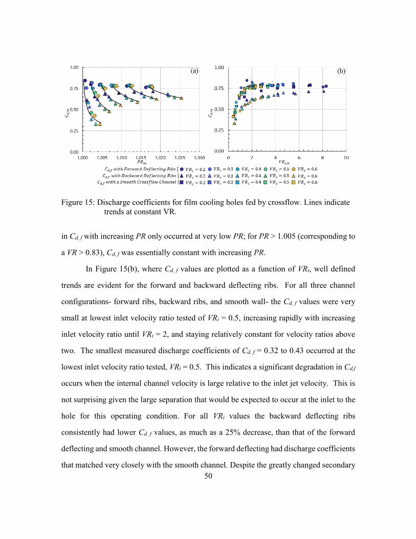
50

in Cd, f with increasing PR only occurred at very low PR; for PR > 1.005 (corresponding to

a VR > 0.83), Cd, f was essentially constant with increasing PR.

In Figure 15(b), where Cd, f values are plotted as a function of VRi, well defined

trends are evident for the forward and backward deflecting ribs. For all three channel

configurations- forward ribs, backward ribs, and smooth wall- the Cd, f values were very

small at lowest inlet velocity ratio tested of VRi = 0.5, increasing rapidly with increasing

inlet velocity ratio until VRi = 2, and staying relatively constant for velocity ratios above

two. The smallest measured discharge coefficients of Cd, f = 0.32 to 0.43 occurred at the

lowest inlet velocity ratio tested, VRi = 0.5. This indicates a significant degradation in Cd,f

occurs when the internal channel velocity is large relative to the inlet jet velocity. This is

not surprising given the large separation that would be expected to occur at the inlet to the

hole for this operating condition. For all VRi values the backward deflecting ribs

consistently had lower Cd, f values, as much as a 25% decrease, than that of the forward

deflecting and smooth channel. However, the forward deflecting had discharge coefficients

that matched very closely with the smooth channel. Despite the greatly changed secondary

Figure 15: Discharge coefficients for film cooling holes fed by crossflow. Lines indicate

trends at constant VR.

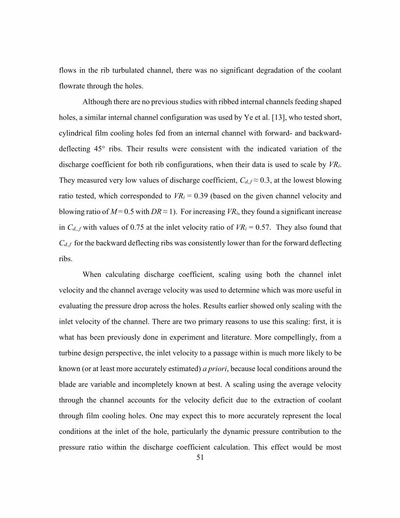
51

flows in the rib turbulated channel, there was no significant degradation of the coolant

flowrate through the holes.

Although there are no previous studies with ribbed internal channels feeding shaped

holes, a similar internal channel configuration was used by Ye et al. [13], who tested short,

cylindrical film cooling holes fed from an internal channel with forward- and backward-

deflecting 45° ribs. Their results were consistent with the indicated variation of the

discharge coefficient for both rib configurations, when their data is used to scale by VRi.

They measured very low values of discharge coefficient, Cd,,f ≈ 0.3, at the lowest blowing

ratio tested, which corresponded to VRi = 0.39 (based on the given channel velocity and

blowing ratio of M = 0.5 with DR ≈ 1). For increasing VRi, they found a significant increase

in Cd,,,f with values of 0.75 at the inlet velocity ratio of VRi = 0.57. They also found that

Cd,,f for the backward deflecting ribs was consistently lower than for the forward deflecting

ribs.

When calculating discharge coefficient, scaling using both the channel inlet

velocity and the channel average velocity was used to determine which was more useful in

evaluating the pressure drop across the holes. Results earlier showed only scaling with the

inlet velocity of the channel. There are two primary reasons to use this scaling: first, it is

what has been previously done in experiment and literature. More compellingly, from a

turbine design perspective, the inlet velocity to a passage within is much more likely to be

known (or at least more accurately estimated) a priori, because local conditions around the

blade are variable and incompletely known at best. A scaling using the average velocity

through the channel accounts for the velocity deficit due to the extraction of coolant

through film cooling holes. One may expect this to more accurately represent the local

conditions at the inlet of the hole, particularly the dynamic pressure contribution to the

pressure ratio within the discharge coefficient calculation. This effect would be most

52

pronounced at high extraction ratios- where the film cooling mass flowrate is large relative

to the velocity of the crossflow, lowering the dynamic pressure.

However, demonstrated in Figure 16, the difference between average and inlet

velocity scaling makes little difference to the general shape of the discharge coefficient

curve for a given channel configuration. Scaling the inlet velocity ratio with the same

average velocity has a greater effect, increasing VRi with increasing extraction ratio. This

does not change the trend that Cd,,f plateaus – at a value of ~0.77 for holes with a forward

deflecting rib channel and 0.70 for holes with a backward deflecting rib channel – as VRi

increases. One interesting consequence of the scaling with average channel velocity is that

the behavior of the smooth channel mirrors that of the backward deflecting ribs at low VRi,

but at high VRi the smooth channel behaves similarly to the forward deflecting ribs. The

difference between the smooth channel scaling of the discharge coefficient is primarily due

to the difference in extraction ratios between the different channel configurations. Since

Figure 16:Scaling discharge coefficient with (a) average and (b) inlet channel velocity

53

the rib turbulator measurements were performed with 5mm holes, and the smooth channel

measurements were performed with 4 mm holes, the extraction ratios are often significantly

higher for the rib turbulator cases.

4.2 – CHANNEL FRICTION FACTOR

Friction factor, f, provides a measure of pressure losses for flow in the internal

channel. The friction factor for smooth channels is well established. However, the effects

of rib turbulators and the extraction of fluid through film cooling holes significantly alter

f. Figure 17 shows the friction factors measured for this test, as well as previously

unpublished friction factors from McClintic et al. [9]. These are shown in Figure 17 (a) as

a function of the average channel Reynolds number, Rec,avg (the Reynolds number based

on the average channel velocity, accounting for extraction of fluid through the film cooling

holes) and in Figure 17(b) as a function of VRi. Each is a semi-log plot with friction factor

on the log scale, with favg based on the average channel velocity and fin based on the channel

inlet velocity. Additionally, in Figure 17(a) is the Colebrook correlation for turbulent

internal flow [28]:

1

√𝑓= −2.0 log (

𝑒 𝑑⁄

3.7+

2.51

𝑅𝑒√𝑓)

Clear from these two figures is the substantially larger friction factor for the channel

flow with rib turbulators, with generally a factor of five increase. The large increase in

friction factor is expected for a ribbed channel flow, shown in the the work by Han et al.

[10]. On the Rec,avg plot, distinct groupings of favg are evident, which correspond to constant

VRc. For constant VRc, favg decreased with increasing VR. This is expected, as an increase

in extraction from the channel will reduce the velocity through the channel, leading to a

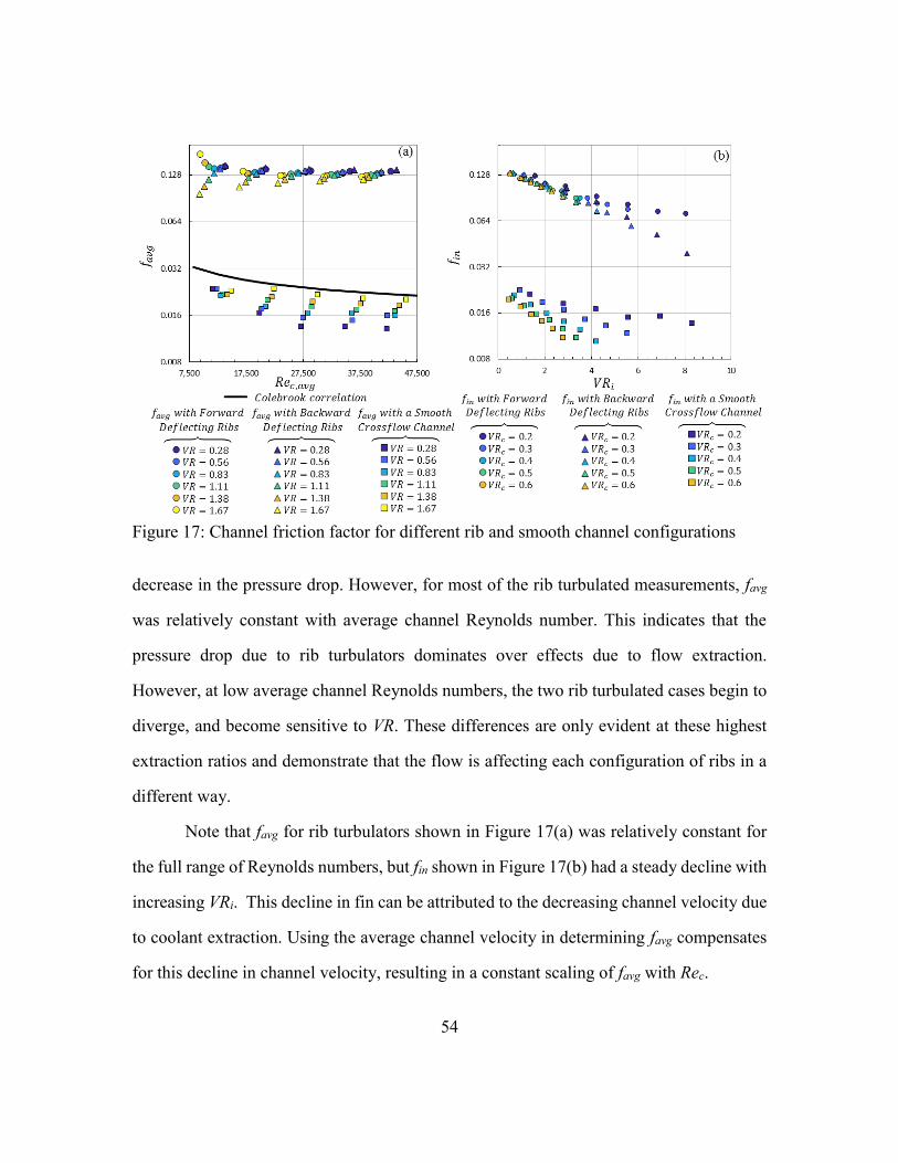
54

decrease in the pressure drop. However, for most of the rib turbulated measurements, favg

was relatively constant with average channel Reynolds number. This indicates that the

pressure drop due to rib turbulators dominates over effects due to flow extraction.

However, at low average channel Reynolds numbers, the two rib turbulated cases begin to

diverge, and become sensitive to VR. These differences are only evident at these highest

extraction ratios and demonstrate that the flow is affecting each configuration of ribs in a

different way.

Note that favg for rib turbulators shown in Figure 17(a) was relatively constant for

the full range of Reynolds numbers, but fin shown in Figure 17(b) had a steady decline with

increasing VRi. This decline in fin can be attributed to the decreasing channel velocity due

to coolant extraction. Using the average channel velocity in determining favg compensates

for this decline in channel velocity, resulting in a constant scaling of favg with Rec.

Figure 17: Channel friction factor for different rib and smooth channel configurations

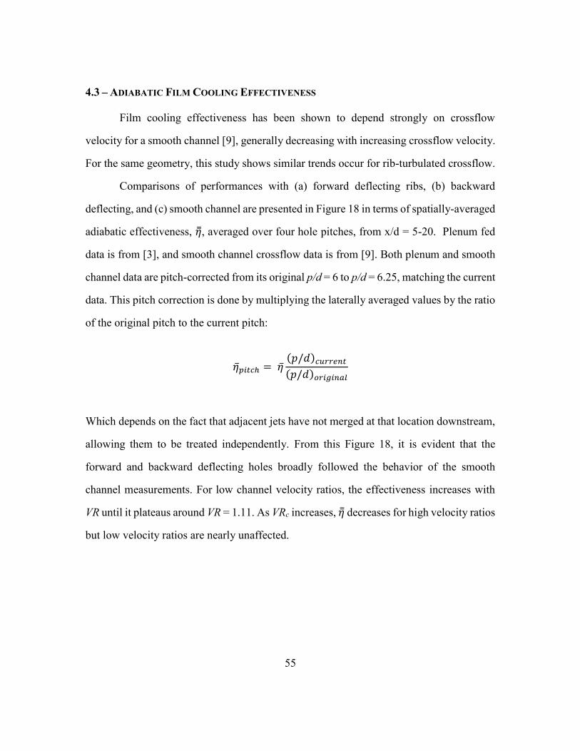
55

4.3 – ADIABATIC FILM COOLING EFFECTIVENESS

Film cooling effectiveness has been shown to depend strongly on crossflow

velocity for a smooth channel [9], generally decreasing with increasing crossflow velocity.

For the same geometry, this study shows similar trends occur for rib-turbulated crossflow.

Comparisons of performances with (a) forward deflecting ribs, (b) backward

deflecting, and (c) smooth channel are presented in Figure 18 in terms of spatially-averaged

adiabatic effectiveness, �̿�, averaged over four hole pitches, from x/d = 5-20. Plenum fed

data is from [3], and smooth channel crossflow data is from [9]. Both plenum and smooth

channel data are pitch-corrected from its original p/d = 6 to p/d = 6.25, matching the current

data. This pitch correction is done by multiplying the laterally averaged values by the ratio

of the original pitch to the current pitch:

�̅�𝑝𝑖𝑡𝑐ℎ = �̅�(𝑝/𝑑)𝑐𝑢𝑟𝑟𝑒𝑛𝑡

(𝑝/𝑑)𝑜𝑟𝑖𝑔𝑖𝑛𝑎𝑙

Which depends on the fact that adjacent jets have not merged at that location downstream,

allowing them to be treated independently. From this Figure 18, it is evident that the

forward and backward deflecting holes broadly followed the behavior of the smooth

channel measurements. For low channel velocity ratios, the effectiveness increases with

VR until it plateaus around VR = 1.11. As VRc increases, �̿� decreases for high velocity ratios

but low velocity ratios are nearly unaffected.

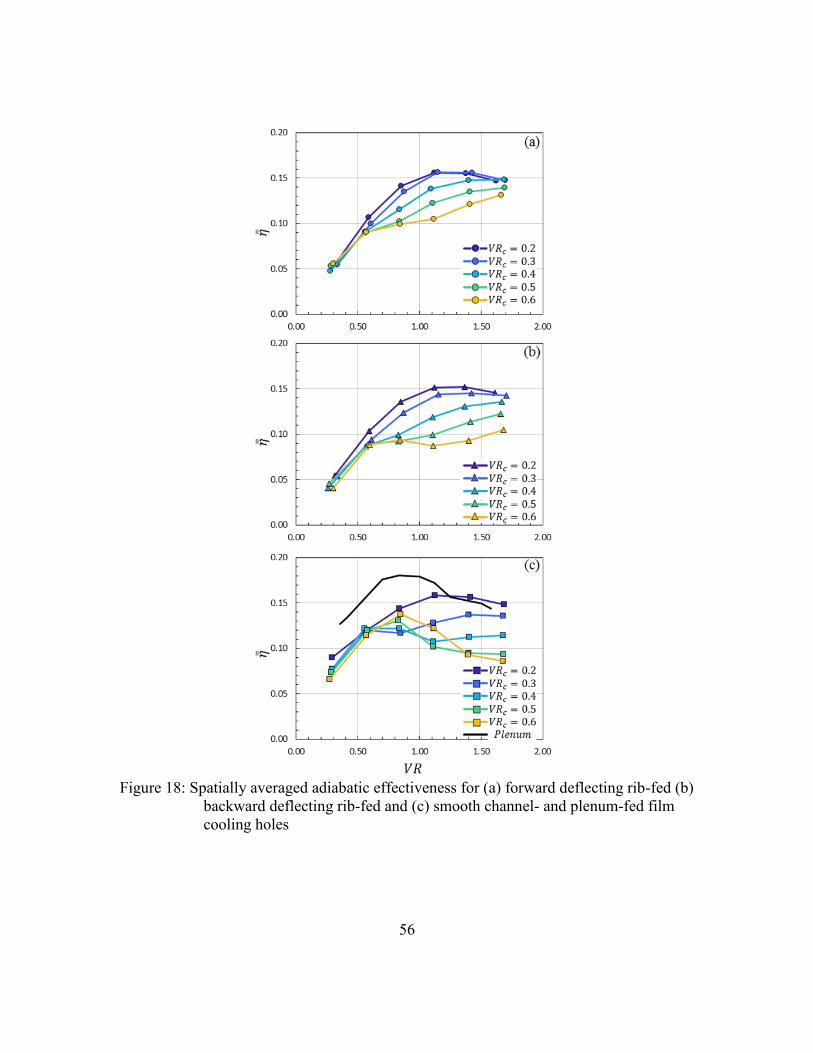
56

Figure 18: Spatially averaged adiabatic effectiveness for (a) forward deflecting rib-fed (b)

backward deflecting rib-fed and (c) smooth channel- and plenum-fed film

cooling holes

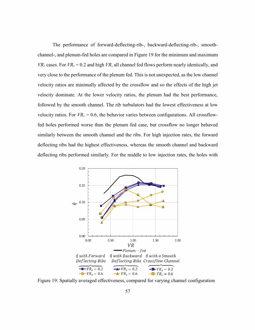
57

The performance of forward-deflecting-rib-, backward-deflecting-rib-, smooth-

channel-, and plenum-fed holes are compared in Figure 19 for the minimum and maximum

VRc cases. For VRc = 0.2 and high VR, all channel fed flows perform nearly identically, and

very close to the performance of the plenum fed. This is not unexpected, as the low channel

velocity ratios are minimally affected by the crossflow and so the effects of the high jet

velocity dominate. At the lower velocity ratios, the plenum had the best performance,

followed by the smooth channel. The rib turbulators had the lowest effectiveness at low

velocity ratios. For VRc = 0.6, the behavior varies between configurations. All crossflow-

fed holes performed worse than the plenum fed case, but crossflow no longer behaved

similarly between the smooth channel and the ribs. For high injection rates, the forward

deflecting ribs had the highest effectiveness, whereas the smooth channel and backward

deflecting ribs performed similarly. For the middle to low injection rates, the holes with

Figure 19: Spatially averaged effectiveness, compared for varying channel configuration

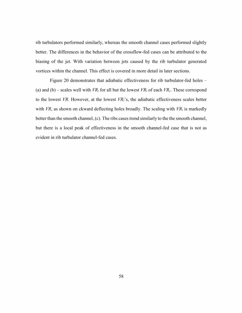
58

rib turbulators performed similarly, whereas the smooth channel cases performed slightly

better. The differences in the behavior of the crossflow-fed cases can be attributed to the

biasing of the jet. With variation between jets caused by the rib turbulator generated

vortices within the channel. This effect is covered in more detail in later sections.

Figure 20 demonstrates that adiabatic effectiveness for rib turbulator-fed holes –

(a) and (b) – scales well with VRi for all but the lowest VRi of each VRc. These correspond

to the lowest VR. However, at the lowest VRi’s, the adiabatic effectiveness scales better

with VR, as shown on ckward deflecting holes broadly. The scaling with VRi is markedly

better than the smooth channel, (c). The ribs cases trend similarly to the the smooth channel,

but there is a local peak of effectiveness in the smooth channel-fed case that is not as

evident in rib turbulator channel-fed cases.

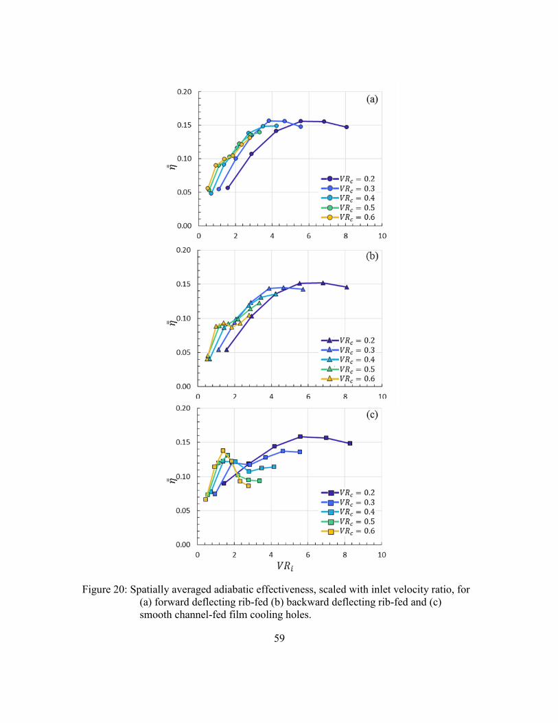
59

Figure 20: Spatially averaged adiabatic effectiveness, scaled with inlet velocity ratio, for

(a) forward deflecting rib-fed (b) backward deflecting rib-fed and (c)

smooth channel-fed film cooling holes.

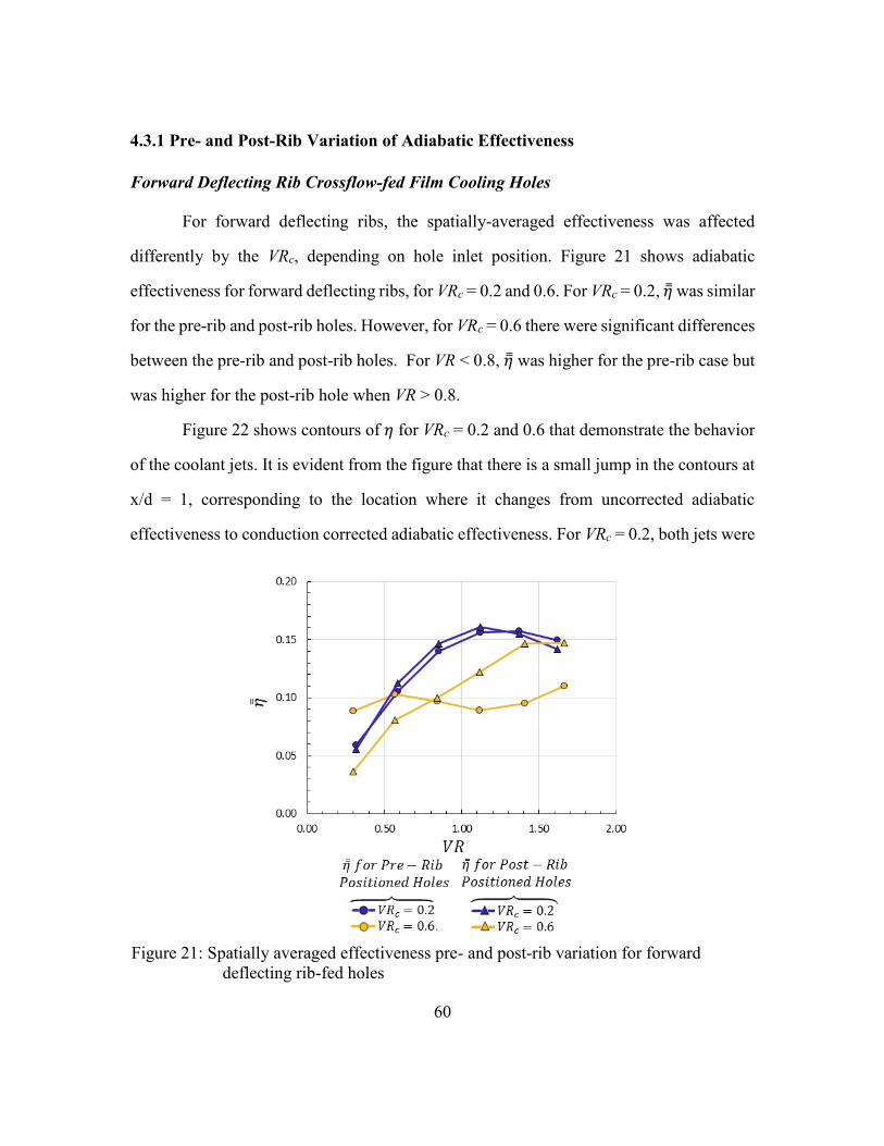
60

4.3.1 Pre- and Post-Rib Variation of Adiabatic Effectiveness

Forward Deflecting Rib Crossflow-fed Film Cooling Holes

For forward deflecting ribs, the spatially-averaged effectiveness was affected

differently by the VRc, depending on hole inlet position. Figure 21 shows adiabatic

effectiveness for forward deflecting ribs, for VRc = 0.2 and 0.6. For VRc = 0.2, �̿� was similar

for the pre-rib and post-rib holes. However, for VRc = 0.6 there were significant differences

between the pre-rib and post-rib holes. For VR < 0.8, �̿� was higher for the pre-rib case but

was higher for the post-rib hole when VR > 0.8.

Figure 22 shows contours of 𝜂 for VRc = 0.2 and 0.6 that demonstrate the behavior

of the coolant jets. It is evident from the figure that there is a small jump in the contours at

x/d = 1, corresponding to the location where it changes from uncorrected adiabatic

effectiveness to conduction corrected adiabatic effectiveness. For VRc = 0.2, both jets were

Figure 21: Spatially averaged effectiveness pre- and post-rib variation for forward

deflecting rib-fed holes

61

very similar at the hole exit resulting in similar adiabatic effectiveness. The crossflow in

this case was not strong enough to significantly bias the jet, so any variation of the hole

inlet position relative to the rib had negligible effect on performance.

However, for VRc = 0.6 there were two effects that changed the adiabatic

effectiveness. At low injection rates, the contour indicates that there was simply more

coolant coming from the pre-rib hole than the post-rib hole. The only other explanation for

decreasing effectiveness would be jet separation from the wall, which is highly unlikely at

these low velocity ratios. The post-rib separation lies over the inlet of the post-rib

positioned hole, creating a local low-pressure region over the hole. This effectively

decreases the pressure ratio and velocity ratio for that hole. This effect was only evident

Figure 22: Contours of forward deflecting rib-fed shaped hole effectiveness

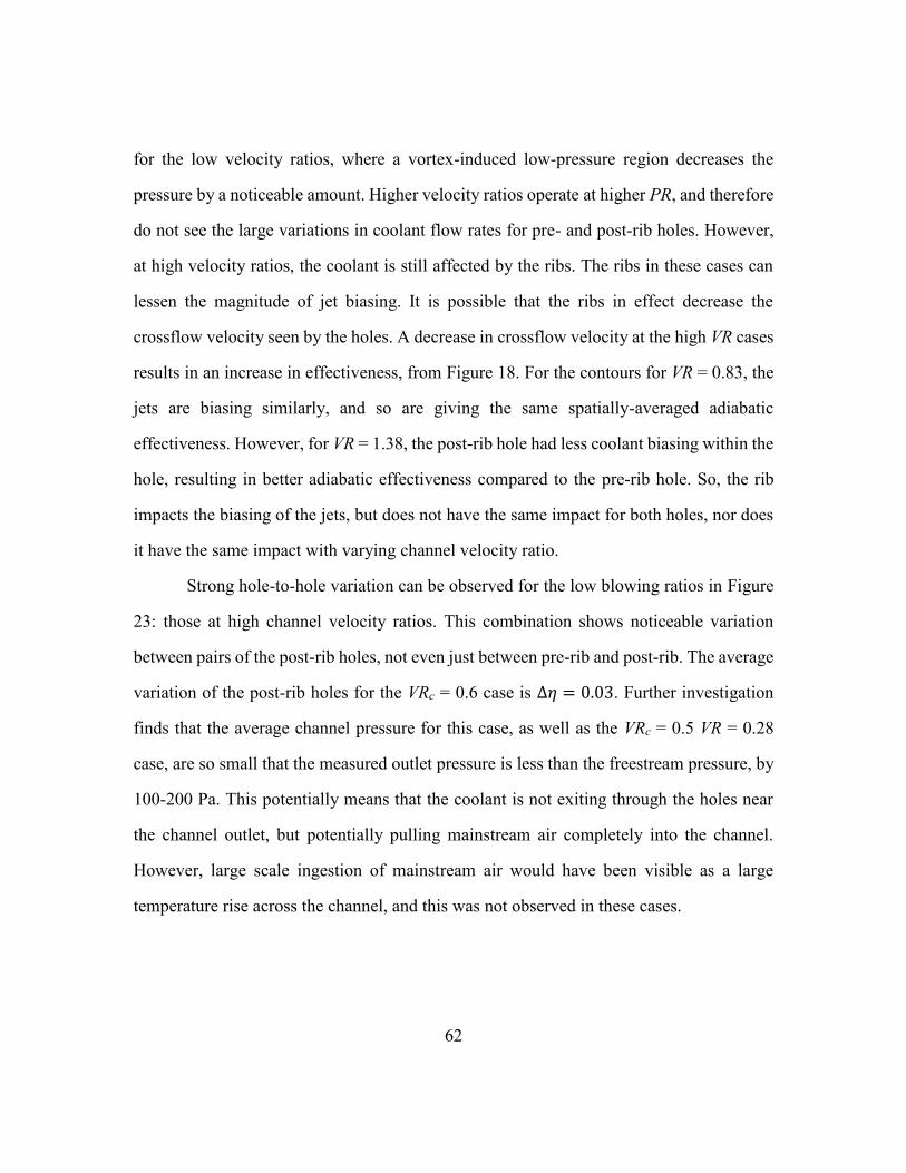
62

for the low velocity ratios, where a vortex-induced low-pressure region decreases the

pressure by a noticeable amount. Higher velocity ratios operate at higher PR, and therefore

do not see the large variations in coolant flow rates for pre- and post-rib holes. However,

at high velocity ratios, the coolant is still affected by the ribs. The ribs in these cases can

lessen the magnitude of jet biasing. It is possible that the ribs in effect decrease the

crossflow velocity seen by the holes. A decrease in crossflow velocity at the high VR cases

results in an increase in effectiveness, from Figure 18. For the contours for VR = 0.83, the

jets are biasing similarly, and so are giving the same spatially-averaged adiabatic

effectiveness. However, for VR = 1.38, the post-rib hole had less coolant biasing within the

hole, resulting in better adiabatic effectiveness compared to the pre-rib hole. So, the rib

impacts the biasing of the jets, but does not have the same impact for both holes, nor does

it have the same impact with varying channel velocity ratio.

Strong hole-to-hole variation can be observed for the low blowing ratios in Figure

23: those at high channel velocity ratios. This combination shows noticeable variation

between pairs of the post-rib holes, not even just between pre-rib and post-rib. The average

variation of the post-rib holes for the VRc = 0.6 case is ∆𝜂 = 0.03. Further investigation

finds that the average channel pressure for this case, as well as the VRc = 0.5 VR = 0.28

case, are so small that the measured outlet pressure is less than the freestream pressure, by

100-200 Pa. This potentially means that the coolant is not exiting through the holes near

the channel outlet, but potentially pulling mainstream air completely into the channel.

However, large scale ingestion of mainstream air would have been visible as a large

temperature rise across the channel, and this was not observed in these cases.

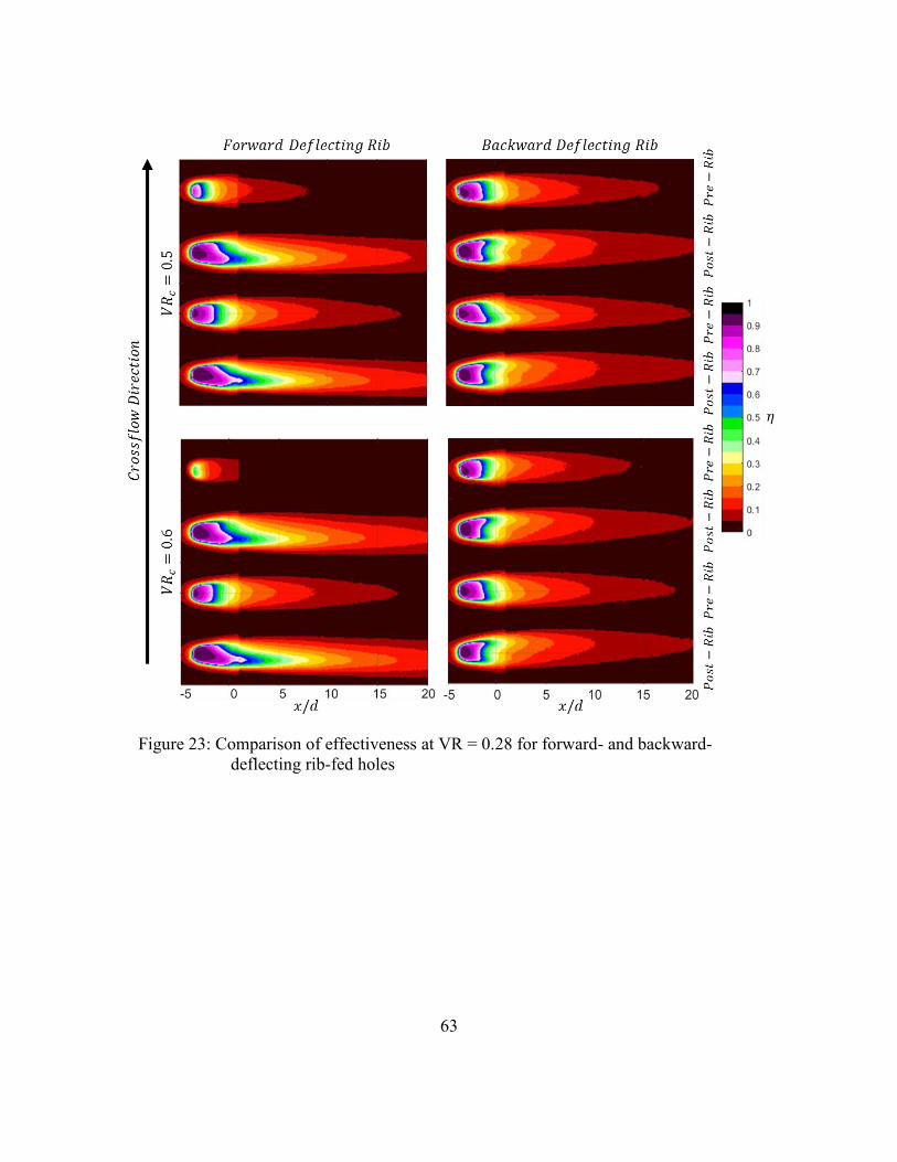
63

Figure 23: Comparison of effectiveness at VR = 0.28 for forward- and backward-

deflecting rib-fed holes

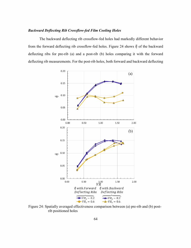
64

Backward Deflecting Rib Crossflow-fed Film Cooling Holes

The backward deflecting rib crossflow-fed holes had markedly different behavior

from the forward deflecting rib crossflow-fed holes. Figure 24 shows �̿� of the backward

deflecting ribs for pre-rib (a) and a post-rib (b) holes comparing it with the forward

deflecting rib measurements. For the post-rib holes, both forward and backward deflecting

Figure 24: Spatially averaged effectiveness comparison between (a) pre-rib and (b) post-

rib positioned holes

65

ribs had the same trend at both VRc = 0.2 and VRc = 0.6. However, the pre-rib holes had

significant differences at high channel velocity ratios, where the holes with the forward

deflecting rib crossflow channel generally outperformed the backward deflecting ribs.

Comparisons between pre-rib and post-rib cases for the backward deflecting rib

crossflow-fed holes are presented in Figure 25. These results show that with VRc = 0.2, the

rib turbulator cases performed the same. But for VRc = 0.6 the pre- and post-rib cases are

quite different, with the post-rib fed holes providing significantly better adiabatic

effectiveness than the pre-rib holes. Similar to the results of the forward deflecting rib

configuration, this could be caused by the post-rib vortex over the inlet to the hole,

mitigating the biasing due to the high crossflow velocity.

The contours of 𝜂 presented in Figure 26 provide some insight into the cause: at

VRc = 0.2, the adiabatic effectiveness for pre- and post-rib holes had little skewness at the

exit of the holes and consequently had very similar performance. For VRc = 0.6 and VR =

Figure 25: Spatially averaged effectiveness pre- and post-rib variation for backward

deflecting rib-fed holes

66

1.38, the adiabatic effectiveness for pre-rib holes was strongly skewed to one side of the

coolant hole, resulting in much poorer performance than for the post-rib hole. From Figure

28(a), this condition corresponds to the peak in jet bias for the smooth channel fed holes.

This is an indication that the strength of jet bias is mitigated for the post-rib inlet location,

whereas the pre-rib hole is less protected from the crossflow’s biasing effect.

4.3.2 – Jet Bias Parameters of Adiabatic Effectiveness

A useful metric to quantify the extent of bias of the coolant jets is quantifying the

location of peak effectiveness, (z/d)CL. Averaged values of so called “centerline location”

from x/d = 5-25 are shown in Figure 27 as a function of VRi, for (a) the pre-rib hole and (b)

Figure 26: Contours of backward deflecting rib-fed shaped hole effectiveness

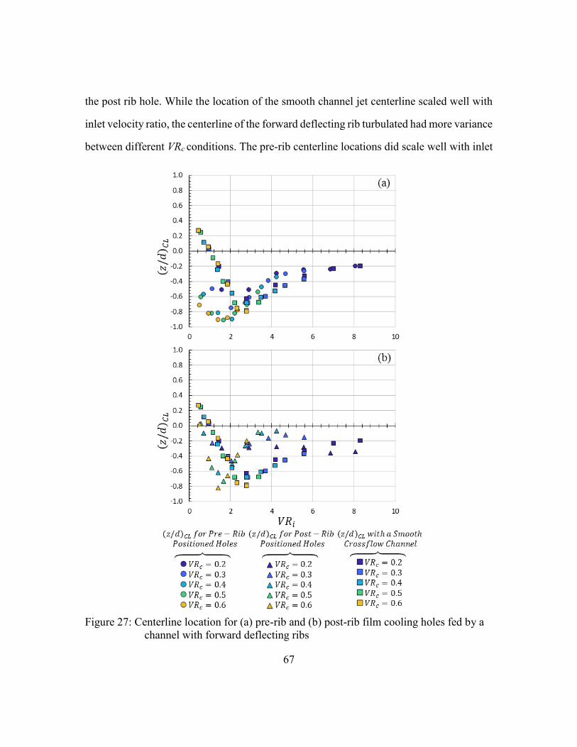
67

the post rib hole. While the location of the smooth channel jet centerline scaled well with

inlet velocity ratio, the centerline of the forward deflecting rib turbulated had more variance

between different VRc conditions. The pre-rib centerline locations did scale well with inlet

Figure 27: Centerline location for (a) pre-rib and (b) post-rib film cooling holes fed by a

channel with forward deflecting ribs

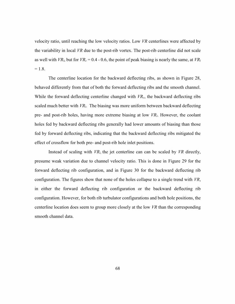
68

velocity ratio, until reaching the low velocity ratios. Low VR centerlines were affected by

the variability in local VR due to the post-rib vortex. The post-rib centerline did not scale

as well with VRi, but for VRc = 0.4 - 0.6, the point of peak biasing is nearly the same, at VRi

= 1.8.

The centerline location for the backward deflecting ribs, as shown in Figure 28,

behaved differently from that of both the forward deflecting ribs and the smooth channel.

While the forward deflecting centerline changed with VRc, the backward deflecting ribs

scaled much better with VRi. The biasing was more uniform between backward deflecting

pre- and post-rib holes, having more extreme biasing at low VRi. However, the coolant

holes fed by backward deflecting ribs generally had lower amounts of biasing than those

fed by forward deflecting ribs, indicating that the backward deflecting ribs mitigated the

effect of crossflow for both pre- and post-rib hole inlet positions.

Instead of scaling with VRi, the jet centerline can can be scaled by VR directly,

presume weak variation due to channel velocity ratio. This is done in Figure 29 for the

forward deflecting rib configuration, and in Figure 30 for the backward deflecting rib

configuration. The figures show that none of the holes collapse to a single trend with VR,

in either the forward deflecting rib configuration or the backward deflecting rib

configuration. However, for both rib turbulator configurations and both hole positions, the

centerline location does seem to group more closely at the low VR than the corresponding

smooth channel data.

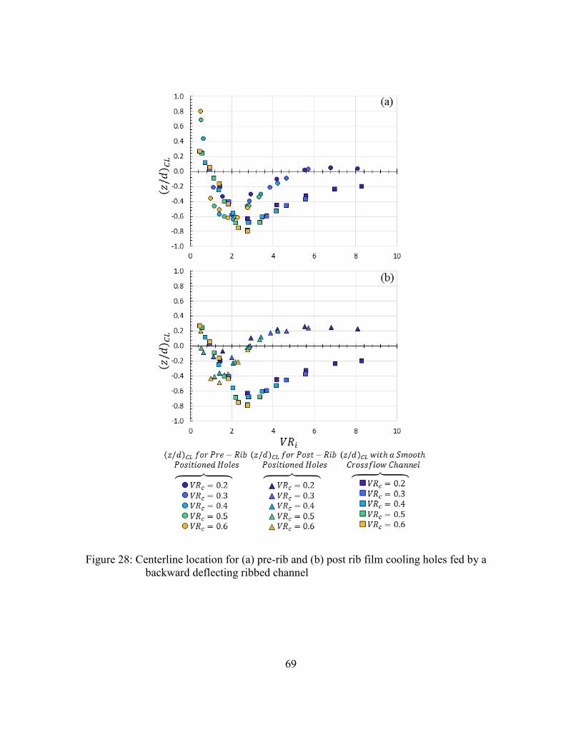
69

Figure 28: Centerline location for (a) pre-rib and (b) post rib film cooling holes fed by a

backward deflecting ribbed channel

70

Figure 29: Centerline location scaled with VR for (a) pre-rib holes fed by a channel with

forward deflecting ribs, (b) post-rib holes fed by a channel with forward

deflecting ribs (c) holes fed by smooth channel

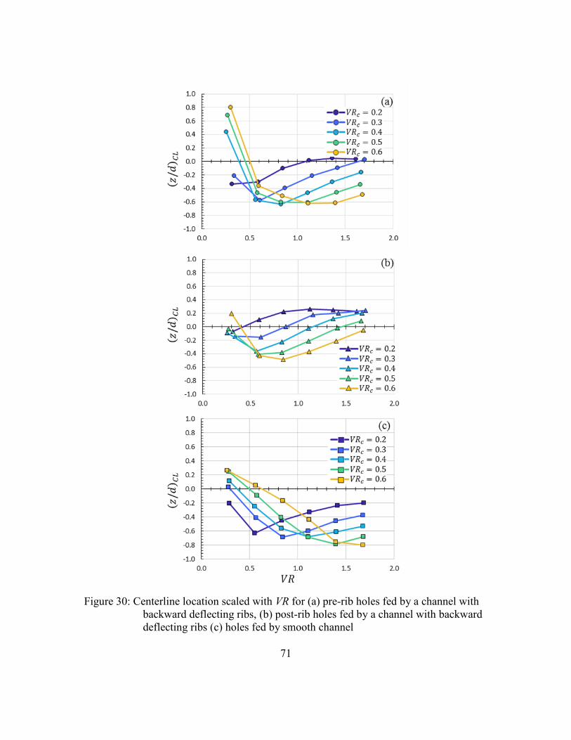
71

Figure 30: Centerline location scaled with VR for (a) pre-rib holes fed by a channel with

backward deflecting ribs, (b) post-rib holes fed by a channel with backward

deflecting ribs (c) holes fed by smooth channel

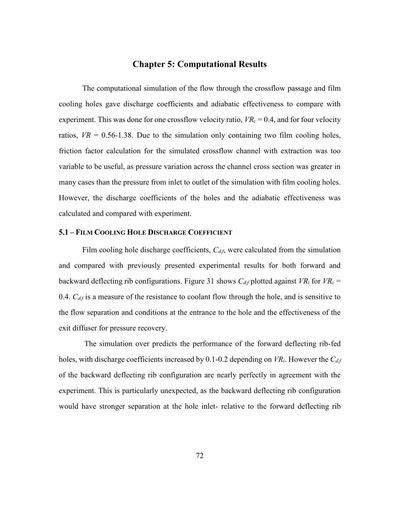
72

Chapter 5: Computational Results

The computational simulation of the flow through the crossflow passage and film

cooling holes gave discharge coefficients and adiabatic effectiveness to compare with

experiment. This was done for one crossflow velocity ratio, VRc = 0.4, and for four velocity

ratios, VR = 0.56-1.38. Due to the simulation only containing two film cooling holes,

friction factor calculation for the simulated crossflow channel with extraction was too

variable to be useful, as pressure variation across the channel cross section was greater in

many cases than the pressure from inlet to outlet of the simulation with film cooling holes.

However, the discharge coefficients of the holes and the adiabatic effectiveness was

calculated and compared with experiment.

5.1 – FILM COOLING HOLE DISCHARGE COEFFICIENT

Film cooling hole discharge coefficients, Cd,f, were calculated from the simulation

and compared with previously presented experimental results for both forward and

backward deflecting rib configurations. Figure 31 shows Cd,f plotted against VRi for VRc =

0.4. Cd,f is a measure of the resistance to coolant flow through the hole, and is sensitive to

the flow separation and conditions at the entrance to the hole and the effectiveness of the

exit diffuser for pressure recovery.

The simulation over predicts the performance of the forward deflecting rib-fed

holes, with discharge coefficients increased by 0.1-0.2 depending on VRi. However the Cd,f

of the backward deflecting rib configuration are nearly perfectly in agreement with the

experiment. This is particularly unexpected, as the backward deflecting rib configuration

would have stronger separation at the hole inlet- relative to the forward deflecting rib

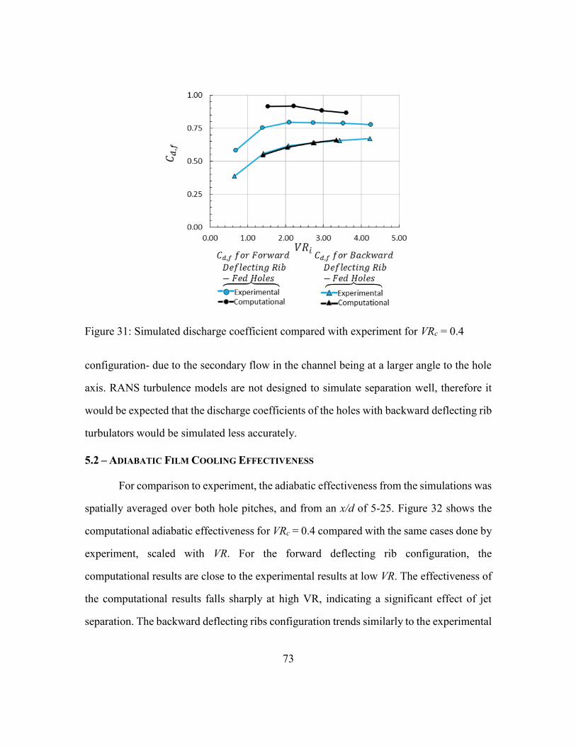
73

configuration- due to the secondary flow in the channel being at a larger angle to the hole

axis. RANS turbulence models are not designed to simulate separation well, therefore it

would be expected that the discharge coefficients of the holes with backward deflecting rib

turbulators would be simulated less accurately.

5.2 – ADIABATIC FILM COOLING EFFECTIVENESS

For comparison to experiment, the adiabatic effectiveness from the simulations was

spatially averaged over both hole pitches, and from an x/d of 5-25. Figure 32 shows the

computational adiabatic effectiveness for VRc = 0.4 compared with the same cases done by

experiment, scaled with VR. For the forward deflecting rib configuration, the

computational results are close to the experimental results at low VR. The effectiveness of

the computational results falls sharply at high VR, indicating a significant effect of jet

separation. The backward deflecting ribs configuration trends similarly to the experimental

Figure 31: Simulated discharge coefficient compared with experiment for VRc = 0.4

74

results, but over predicts effectiveness for the middle two VR cases simulated. In both

configurations, the effectiveness peaks at a lower VR, indicating the possibility of early

separation of the jet.

5.2.1 – Effectiveness of Forward Deflecting Rib-Fed Holes

Focusing on the forward deflecting rib configuration, the results can be better

understood by splitting the overall average of adiabatic effectiveness into a pre-rib

positioned hole and a post-rib positioned hole. This split is compared in Figure 33 to the

effectiveness from experiment. It is clear is that the simulation exhibits much greater

variability between pre-rib and post-rib positioned holes. The pre-rib hole begins much

higher than the experiment and the computational post-rib hole but falls sharply with

increasing VR. This is the primary reason why the effectiveness in Figure 32 falls off in

the high VR cases. Additionally, the experiment predicts that the pre-rib positioned holes

Figure 32: Contours of effectiveness for forward deflecting rib crossflow-fed holes, at a

VRc = 0.4

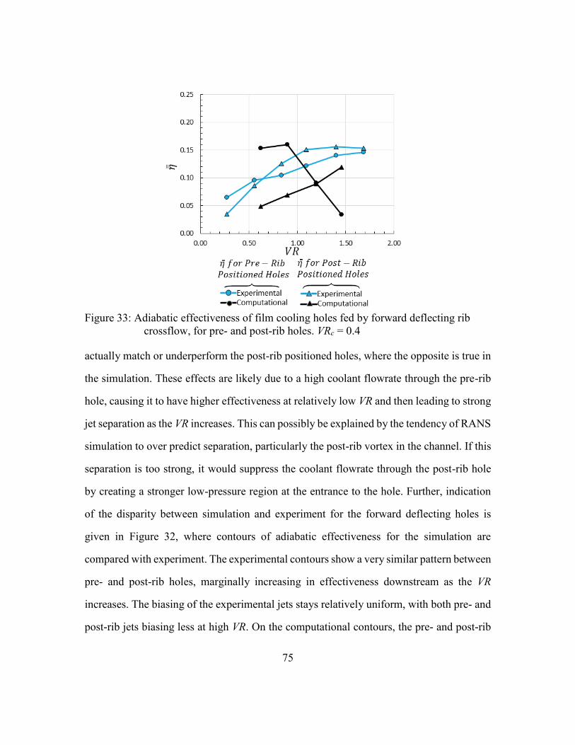
75

actually match or underperform the post-rib positioned holes, where the opposite is true in

the simulation. These effects are likely due to a high coolant flowrate through the pre-rib

hole, causing it to have higher effectiveness at relatively low VR and then leading to strong

jet separation as the VR increases. This can possibly be explained by the tendency of RANS

simulation to over predict separation, particularly the post-rib vortex in the channel. If this

separation is too strong, it would suppress the coolant flowrate through the post-rib hole

by creating a stronger low-pressure region at the entrance to the hole. Further, indication

of the disparity between simulation and experiment for the forward deflecting holes is

given in Figure 32, where contours of adiabatic effectiveness for the simulation are

compared with experiment. The experimental contours show a very similar pattern between

pre- and post-rib holes, marginally increasing in effectiveness downstream as the VR

increases. The biasing of the experimental jets stays relatively uniform, with both pre- and

post-rib jets biasing less at high VR. On the computational contours, the pre- and post-rib

Figure 33: Adiabatic effectiveness of film cooling holes fed by forward deflecting rib

crossflow, for pre- and post-rib holes. VRc = 0.4

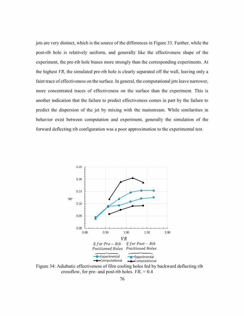
76

jets are very distinct, which is the source of the differences in Figure 33. Further, while the

post-rib hole is relatively uniform, and generally like the effectiveness shape of the

experiment, the pre-rib hole biases more strongly than the corresponding experiments. At

the highest VR, the simulated pre-rib hole is clearly separated off the wall, leaving only a

faint trace of effectiveness on the surface. In general, the computational jets leave narrower,

more concentrated traces of effectiveness on the surface than the experiment. This is

another indication that the failure to predict effectiveness comes in part by the failure to

predict the dispersion of the jet by mixing with the mainstream. While similarities in

behavior exist between computation and experiment, generally the simulation of the

forward deflecting rib configuration was a poor approximation to the experimental test.

Figure 34: Adiabatic effectiveness of film cooling holes fed by backward deflecting rib

crossflow, for pre- and post-rib holes. VRc = 0.4

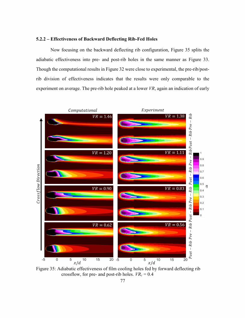
77

5.2.2 – Effectiveness of Backward Deflecting Rib-Fed Holes

Now focusing on the backward deflecting rib configuration, Figure 35 splits the

adiabatic effectiveness into pre- and post-rib holes in the same manner as Figure 33.

Though the computational results in Figure 32 were close to experimental, the pre-rib/post-

rib division of effectiveness indicates that the results were only comparable to the

experiment on average. The pre-rib hole peaked at a lower VR, again an indication of early

Figure 35: Adiabatic effectiveness of film cooling holes fed by forward deflecting rib

crossflow, for pre- and post-rib holes. VRc = 0.4

78

separation of the jet. However, the post-rib hole simulation did match similar trends to the

experiment, particularly as the post-rib hole flattens out when approaching high VR.

The backward deflecting rib simulation can be further compared with experiment

with the contours of effectiveness in Figure 36. In general, the simulated jets are much

narrower and concentrated, as in the forward deflecting rib configuration. Comparing pre-

rib holes, the bias of the jet is clearly different between simulation and experiment at every

VR. This difference is also evident between the post-rib holes. In fact, the post-rib holes of

the simulation seem to match the centerline location of the experimental pre-rib holes, and

vice-versa. The centerline location differences indicate that the flow field through the hole

is totally different in the simulation, even though the spatial average of effectiveness was

similar. Finally, the computational contours of both Figure 32 and Figure 36 indicate both

significantly higher centerline effectiveness and narrower jets, which primarily a failure of

the gradient diffusion hypothesis. In effect, this transport hypothesis under predicts the

mixing of the jet into the mainstream, leading to a more concentrated, narrower trace of

effectiveness downstream.

Through this film cooling simulation, it is made clear that assumptions of this

RANS model are not sufficient for accurately capturing the complex rib-turbulated

crossflow film cooling flow field. Originally formulated for boundary layer simulation, the

k-ε turbulence model is notably poor at handling separated flow regions. Since these occur

both post-rib inside the channel, and within the entrance of the hole and at the diffuser, it

is not surprising that the flow field is not accurate. Compounding the turbulent closure

problem is that of the temperature transport; the gradient diffusion hypothesis for

conserved passive scalar transport evidently under predicts the mixing and spread of the

jet as it interacts with the mainstream.

79

Figure 36: Contours of effectiveness for backward deflecting rib crossflow-fed holes

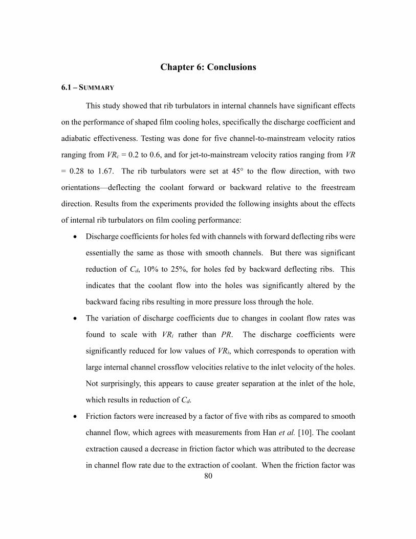
80

Chapter 6: Conclusions

6.1 – SUMMARY

This study showed that rib turbulators in internal channels have significant effects

on the performance of shaped film cooling holes, specifically the discharge coefficient and

adiabatic effectiveness. Testing was done for five channel-to-mainstream velocity ratios

ranging from VRc = 0.2 to 0.6, and for jet-to-mainstream velocity ratios ranging from VR

= 0.28 to 1.67. The rib turbulators were set at 45° to the flow direction, with two

orientations—deflecting the coolant forward or backward relative to the freestream

direction. Results from the experiments provided the following insights about the effects

of internal rib turbulators on film cooling performance:

• Discharge coefficients for holes fed with channels with forward deflecting ribs were

essentially the same as those with smooth channels. But there was significant

reduction of Cd, 10% to 25%, for holes fed by backward deflecting ribs. This

indicates that the coolant flow into the holes was significantly altered by the

backward facing ribs resulting in more pressure loss through the hole.

• The variation of discharge coefficients due to changes in coolant flow rates was

found to scale with VRi rather than PR. The discharge coefficients were

significantly reduced for low values of VRi, which corresponds to operation with

large internal channel crossflow velocities relative to the inlet velocity of the holes.

Not surprisingly, this appears to cause greater separation at the inlet of the hole,

which results in reduction of Cd.

• Friction factors were increased by a factor of five with ribs as compared to smooth

channel flow, which agrees with measurements from Han et al. [10]. The coolant

extraction caused a decrease in friction factor which was attributed to the decrease

in channel flow rate due to the extraction of coolant. When the friction factor was

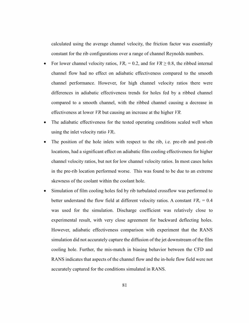
81

calculated using the average channel velocity, the friction factor was essentially

constant for the rib configurations over a range of channel Reynolds numbers.

• For lower channel velocity ratios, VRc = 0.2, and for VR ≥ 0.8, the ribbed internal

channel flow had no effect on adiabatic effectiveness compared to the smooth

channel performance. However, for high channel velocity ratios there were

differences in adiabatic effectiveness trends for holes fed by a ribbed channel

compared to a smooth channel, with the ribbed channel causing a decrease in

effectiveness at lower VR but causing an increase at the higher VR.

• The adiabatic effectiveness for the tested operating conditions scaled well when

using the inlet velocity ratio VRi.

• The position of the hole inlets with respect to the rib, i.e. pre-rib and post-rib

locations, had a significant effect on adiabatic film cooling effectiveness for higher

channel velocity ratios, but not for low channel velocity ratios. In most cases holes

in the pre-rib location performed worse. This was found to be due to an extreme

skewness of the coolant within the coolant hole.

• Simulation of film cooling holes fed by rib turbulated crossflow was performed to

better understand the flow field at different velocity ratios. A constant VRc = 0.4

was used for the simulation. Discharge coefficient was relatively close to

experimental result, with very close agreement for backward deflecting holes.

However, adiabatic effectiveness comparison with experiment that the RANS

simulation did not accurately capture the diffusion of the jet downstream of the film

cooling hole. Further, the mis-match in biasing behavior between the CFD and

RANS indicates that aspects of the channel flow and the in-hole flow field were not

accurately captured for the conditions simulated in RANS.

82

6.2 – RECOMMENDATIONS FOR FUTURE WORK

Much can be done beyond this work to further the study of rib turbulator fed film

cooling holes. The position of hole entrance relative to the rib can be explored in more

detail, as well as different geometries for both ribs and film cooling holes. The hole

entrance effects set up the biasing of the coolant jet as it exits the hole, ultimately varying

the adiabatic effectiveness. Understanding the complex interaction with rib turbulators can

lead to better designs using the combination of ribs and shaped film cooling holes,

potentially shaping hole inlets to mitigate the biasing effect of crossflow or to better

distribute coolant on the surface at a given channel velocity ratio. Further experimental

investigation of the flow field itself can be done to better understand the rib turbulator flow,

the hole interaction, and the jet downstream. This information can be used to potentially

improve simulation techniques and provide data for comparison with LES or DNS

simulations.

83

References

[1] Bunker, R.S., 2017, “Evolution of Turbine Cooling,” ASME paper No. GT2017-

94174.

[2] Bogard, D. G, Thole, K. A., 2006 “Gas Turbine Film Cooling”, J. Power &

Propulsion,Vol. 22, No. 2, p. 249-270.

[3] Anderson, J. B., 2017, “Investigation of Approach Flow Parameters, Scaling Factors,

and Measurement Accuracy for Film Cooling Effectiveness and Heat Transfer

Coefficient Measurements,” Ph.D. dissertation, Cockrell School of Engineering, The

University of Texas at Austin.

[4] Haydt, S., Lynch, S., Lewis, S., “The Effect of Area Ratio Via Increased Hole Length

for Shaped Film Cooling Holes with Constant Expansion Angles”, ASME Paper No.

GT2017-63692.

[5] Issakhanian, E., Elkins, C. J., Eaton, J. K., “Pitfalls of Fan-Shaped Hole Design:

Insights from Experimental Measurement of In-Hole Flow Through MRV”, ASME

Paper No. GT2017-63679.

[6] Gritsch, M., Schulz, A., and Wittig, S., 2003, “Effect of Internal Coolant Crossflow on

the Effectiveness of Shaped Film-Cooling Holes,” J. Turbomach., 125, pp. 547-554.

[7] Saumweber, C., and Schulz, A., 2008, “Comparison of the Cooling Performance of

Cylindrical and Fan-Shaped Cooling Holes with Special Emphasis on the Effect of

Internal Coolant Cross-Flow,” ASME paper GT2008-51036.

[8] Saumweber, C. and Schulz, A., 2012, “Effect of Geometry Variations on the Cooling

Performance of Fan-Shaped Cooling Holes,” J. Turbomach., Vol 134, p.061008.

[9] McClintic, J.W., 2017, “Diffused-Exit Film Cooling Holes Fed by an Internal

Crossflow”, Ph.D. dissertation, Cockrell School of Engineering, The University of

Texas at Austin.

[10] Han, J. C., Park, J. S., Lei, C. K., 1985, "Heat Transfer Enhancement in Channels with

Turbulence Promoters." J. Eng. Gas Turbines and Power, Vol. 107, pp. 628-635.

[11] Chanteloup, D. Bolcs, A., 2002, "Experimental Investigation of Heat Transfer in Two-

Pass Coolant Pasages With Ribs and Film Cooling Hole Ejection." ASME paper

DETC2002/CIE-34443.

[12] Bunker, R. S. and Bailey, J. C., 2001, “Film Cooling Discharge Coefficient

Measurements in a Turbulated Passage with Internal Crossflow,” J. Turbomach., Vol.

123, pp. 774-780.

[13] Ye, L. Liu, C., Zhu, H. Luo, J. 2017, “Investigations on the Influence of Rib

Orientation Angle on Film Cooling Performance of Cylindrical Holes”, ASME Paper

No. GT2017-63968.

[14] Agata, Y., Takahashi, T., Sakai, E., Nishino, K., 2012, "Effects of Turbulence

Promoters of Gas Turbine Blades on Film Cooling Performance." Thermal Science

and Technology, Vol. 7, No. 4, pp. 603-618.

84

[15] Agata, Y., Takahashi, T., Sakai, E., Nishino, K., 2013, "Effect of Orientation of Internal

Turbulence Promoting Ribs on Flow Characteristics for Film Cooling." Thermal

Science and Technology, Vol. 8, No. 1, pp. 15-27.

[16] Klavetter, S. R., McClintic, J. W., Bogard, D. G, Dees, J., Laskowski, G. M., Briggs,

R. “The Effect of Rib Turbulators on Film Cooling Effectiveness of Round Compound

Angle Holes Fed by and Internal Cross-flow”, ASME Paper No. GT2015-43947.

[17] Walters, D. K., Leylek, J. H., 1997, “A Detailed Analysis of Film-Cooling Physics Part

I: Streamwise Injection with Cylindrical Holes” ASME Paper No. 97-GT-269.

[18] Hyams, D. G., Leylek, J. H., 1997, “A Detailed Analysis of Film-Cooling Physics Part

III: Streamwise Injection with Shaped Holes” ASME Paper No. 97-GT-271.

[19] Leedom, D. H., Acharya, S., 2008, “Large Eddy Simulations of Film Cooling Flow

Fields from Cylindrical and Shaped Holes”, ASME Paper No. GT2008-51009.

[20] Oliver, T. A., Anderson, J. B., Bogard, D. G., Moser, R. D., Laskowski, G., 2017,

“Implicit LES for Shaped-Hole Film Cooling Flow”, ASME Paper No. GT2017-

63314

[21] Kholi, A., Thole, K. A., 1998, “Entrance Effects on Diffused Film-Cooling Holes”

ASME Paper No. 88-GT-402.

[22] Peng, W., Jiang, W. X., 2011, “Experimental and Numerical Study of Film Cooling

with Internal Coolant Cross-Flow Effects” Experimental Heat Transfer, Vol. 25:4, pp.

282-300.

[23] McClintic, J. W., Klavetter, S. R., Anderson, J.B., Winka, J.R., Bogard, D. G, Dees, J.,

Laskowski, G. M., Briggs, R., 2014, “The Effect of Internal Cross-Flow on the

Adiabatic Effectiveness of Compound Angle Film Cooling Holes”, J. Turbomach.,

137:12, pp. 146-152.

[24] Wilkes, E. K., 2015, “The Effect of Channel Parameters on the Adiabatic Film Cooling

Effectiveness of Shaped Holes in Crossflow,” master’s thesis, Cockrell School of

Engineering, The University of Texas at Austin.

[25] Schroeder, R. P. and Thole, K. A., 2014, “Adiabatic Effectiveness Measurements for

a Baseline Shaped Film Cooling Hole,” ASME Paper No. GT2014-25992.

[26] Incropera, F. P., Dewitt, D. P., 1996, Fundamentals of Heat and Mass Transfer, Wiley,

New York, NY, pp. 354-357.

[27] Gritsch, M., Saumweber, C., Schulz, A., Wittig, S., and Sharp, E., 2000, “Effect of

Internal Coolant Crossflow Orientation on the Discharge Coefficient of Shaped Film-

Cooling Holes,” J. Turbomach., 122, pp. 146-152.

[28] Munson, B. R., Young, D. F., Okiishi, T. H., 1990, Fundamentals of Fluid Mechanics,

Wiley, New York, NY, pp. 481, 503.

[29] Moffat, R. J., 1985, "Using Uncertainty Analysis in the Planning of an Experiment,"

J. Fluids Eng., Vol. 107, pp. 121006-1 - 121006-10.

[30] Launder, B.E., Spalding, D. B., 1974, “The Numerical Computation of Turbulent

Flows”, Computer Methods in Applied Mechanics and Engineering, Vol. 3:2, pp.

269-289.

85

[31] Shih, T.H., Liou, W.W., Shabbir, A., Yang, Z., Zhu, J., 1995, “A New k-ϵ Eddy

Viscosity Model for High Reynolds Number Turbulent Flows”, Computers and

Fluids, Vol 24:3, pp. 227-238.

[32] Wolfshtein, M., 1969, “The Velocity and Temperature Distribution in One-

Dimensional Flow with Turbulence Augmentation and Pressure Gradient”

International Journal of Heat and Mass Transfer, Vol 12:3, pp. 301-318.

[33] Jones, F.B., 2018, Graduate Research Assistant, University of Texas at Austin, private

communication.

86

Vita

Dale W. Fox was born in Joliet, Illinois in 1993, and moved to Tulsa, OK and then

West Jordan, UT, before attending the University of Kansas beginning in Fall 2012. He

received his Bachelor of Science in Mechanical Engineering in spring 2016 and

subsequently began graduate work at the University of Texas at Austin in fall 2016. He

joined the Turbulence and Turbine Cooling Research Laboratory, led by Dr. Bogard, that

semester. He completed his Master of Science degree in spring 2018 and intends to

continue work toward his Ph.D. under Dr. Bogard.

Permanent email: dale.fox@utexas.edu

This thesis (report) was typed by the author.