Copyright by Cem Akgüner 2007

Copyright

by

Cem Akgüner

2007

The Dissertation Committee for Cem Akgüner Certifies that this is the approved

version of the following dissertation:

ELASTIC ANALYSIS OF AXIAL LOAD-DISPLACEMENT

BEHAVIOR OF SINGLE DRIVEN PILES

Committee:

Robert B. Gilbert, Supervisor

Roy E. Olson, Co-Supervisor

Michael D. Engelhardt

John M. Sharp, Jr.

Kenneth H. Stokoe II

ELASTIC ANALYSIS OF AXIAL LOAD-DISPLACEMENT

BEHAVIOR OF SINGLE DRIVEN PILES

by

Cem Akgüner, B.S.; M.S.C.E

Dissertation

Presented to the Faculty of the Graduate School of

The University of Texas at Austin

in Partial Fulfillment

of the Requirements

for the Degree of

Doctor of Philosophy

The University of Texas at Austin

December 2007

Dedication

To my dearest family

that I love and care for

who suffered through this process,

made so many sacrifices,

stood by me at all times,

supported me in all possible ways...

you are all one can wish for and dream about...

Life is nothing but a tiresome journey. For a man, it consists of false starts, snail-like

advances, nasty setbacks, and lost collar buttons.

Jean Giraudoux - The Enchanted

Happiness is someone to love, something to do, and something to hope for.

-Chinese Proverb

We know accurately only when we know little, with knowledge doubt increases.

Johann Wolfgang von Goethe, who completed his masterpiece Faust in over 60 years.

v

Acknowledgements

It has truly been a drawn-out process which was followed its own course. This

dissertation could not have been possible without the influence of many individuals who

smoothed the way. Dr. Robert B. Gilbert was the voice of reason and a constant source of

optimism and encouragement as my co-supervisor. He always pointed to the full half of

the cup whenever I focused on the empty portion. His knowledge, keen understanding

and problem-solving skills, generously shared throughout, have been instrumental toward

my completing this dissertation.

My other co-advisor Dr. Roy E. Olson offered me my first and last jobs. Things

have not always been rosy between us, but one thing I could always count on was his

unwavering dedication to engineering, inspiring in-depth knowledge and sense of

perspective at times when my mind and interests would wander. He was always available

and willing to discuss a wide range of topics and to bluntly express his point-of-view. I

sincerely appreciate his support and guidance in my successfully concluding this

dissertation. I will always cherish having worked alongside Dr. Olson.

I would be remiss if I did not thank the other members of my dissertation

committee: Drs. Michael D. Engelhardt, John M. Sharp, Jr., and Kenneth H. Stokoe II. I

am truly grateful for the support they have given to my research using their extensive

knowledge, experience, and wisdom.

Dr. Glen R. Andersen, who was formerly at Texas A&M University and was my

very first advisor, also deserves credit for offering me a chance to work with him. I

learned many important lessons about where one’s priority should lie. Dr. Alan Rauch

also served as my co-supervisor and helped me formulate a rational approach to my

research questions.

vi

I want to thank the warm and helpful UT staff who have had a positive impact on

me and my work: Teresa Tice-Boggs, Vittoria Esile, Evelyn Porter, D.D. Berry, Chris

Treviño, Maximo Treviño, Alicia and Gonzalo Zapata, and Wayne Fontenot. I feel

privileged to have known each and every one of them.

I can not even phantom how my life as a graduate student would have been

without the super, special members of the Engineering Library and Interlibrary Services.

They contributed greatly to my excitement and eagerness to learn and explore new ideas

and approaches.

I must acknowledge some of my amazing fellow geotechies: Mike Myers, Mike

Duffy, Cynthia Finley, Rollins Brown, Elliott Mecham, Celestino Valle, and Beatriz

Camacho. I sincerely benefited from being in an environment where almost everyone is

friendly and genuinely nice to each other. My Korean friends and officemates Dr. Jeong-

Yun Won, Heejung Youn, Boohyun Nam, and Kyu-Seok Woo made me a part of their

close-knit gang and played a very important role for me during the last stages of

writing/correcting/reviewing process of my dissertation. I could not possibly have asked

for a better environment to be in.

I have been extremely lucky and blessed with friends during my stay in Austin,

each of whom has a special place in my heart and mind: Nalan-Ahmet Yakut, Aysu-

Mehmet Darendeli, Rüya-Murat Küçükkaya, Tarkan Yüksel, Cengiz Vural, Cem

Topkaya, Murat Argun, Selim Sakaoğlu, and Tanju Yurtsever. I promise to show my

appreciation to each every time I see them. I want to thank them for letting me be a part

of their lives. I also wronged some people I cared for and I am truly sorry for it.

Over the last five years, there is nobody that I have been closer to than Umut

Beşpınar-Ekici and Özgür Ekici. We have spent much of our free time together, sharing

our thoughts, joys, concerns, walks, frustrations, opinions, movies, prayers, stories, news,

vii

food, and coffee. Özgür has had a refreshing and calming effect on me, although we both

are Gemini. Umut has always found a way to lift my spirits and been first in line to

support me whenever I felt lost or wanted to just give up.

I can not say enough of my family. I would not be where I am right now without

the sacrifices they have made throughout my studies. I am forever indebted to them. My

mother Mary must be canonized as a saint and/or angel with her never-ending optimism,

sunny disposition and intellectual capacity. She has been and will continue to be an

inspiration and a role model for me. I will always remember her yelling, “Adalante! To

Đzmir,” every morning trying to encourage me and keep me going. My father Tayfun has

been a tornado-like driving force, making me strive to continually do my best no matter

what the circumstances are. He is a problem-solver and a go-getter, or, in other words,

the engine that could. My sister Perim has served as the resident child of our family while

I have been gone and done an admirable job. She worked full time while taking a full

load of classes to earn her masters degree, and begin her doctorate, feats which are

simply awe-inspiring to me.

So far so good! Last one to leave should turn-off the lights.

viii

Elastic Analysis of Axial Load-Displacement

Behavior of Single Driven Piles

Publication No._____________

Cem Akgüner, Ph.D.

The University of Texas at Austin, 2007

Co-Supervisors: Robert B. Gilbert and Roy E. Olson

Deep foundations are commonly recommended when large displacements are

expected. Typically, though, their design involves only checking and providing for

sufficient capacity to carry the applied loads. Load-displacement behavior of piles is

considered secondary to the axial capacity; displacements are ordinarily overlooked or

not calculated if and when the estimated pile capacity is two to three times the design or

expected loading. However, in cases, such as long piles or piles in dense cohesionless

soils, displacements can be the critical factor in design or it could be a structural

requirement to limit the displacements.

In this dissertation, the displacements of axially loaded single piles are

investigated by conducting analyses with the aid of an approach based on elasticity. The

original solution predicting displacements due to a vertical load within a semi-infinite soil

mass has been modified for varying soil conditions and layering, and assumptions of

stresses and displacements acting on the soil-pile interface. Aside from the

available/known factors of the pile (length, diameter, cross-sectional area, etc.) and the

ix

layering of the surrounding soil, Young’s modulus and Poisson’s ratio of the soil

encompassing a pile are the unknowns required as input to obtain predictions based on

the elastic method. In this study, attention is directed towards determining Young’s

modulus because the range and variability of Poisson’s ratio is not significant in

displacement calculations.

Axial pile load testing data were provided by the California Department of

Transportation as part of a project to improve its general approach to pile design. All of

the tested piles were driven into the ground. Measurements of displacements and loads

were made only at the top of the pile. Supplementary in-situ testing involving cone

penetration (CPT) and standard penetration (SPT), drilling, and sample collection, were

conducted in addition to laboratory testing to enhance the available information.

In this research, predicted displacements are compared with those deduced from

pile load tests. Two sets of predictions based on elastic method are conducted for

comparing displacements. First, various correlations for Young’s modulus are employed

to determine how accurately each predicts the actual measured displacement. The chosen

correlations utilize laboratory triaxial undrained shear strength and standard penetration

test blowcount for cohesive and cohesionless soils, respectively. Secondly, the same data

are also utilized to obtain back-calculated values of Young’s moduli for analyses

involving the elastic method. The measured displacements at loads of a third, a half, two-

thirds, and equal to the failure load were matched iteratively.

Results from this research are deemed to have an impact on engineering practice

by improving the determination of Young’s modulus for displacement analyses involving

the elastic method. A unique approach that has potential is the reconciliation of load

ratios (percentage of failure load) with displacement calculations to provide a better

overview of the range of load ratios for which these newly formulated correlations may

x

be employed. Through this research, it is anticipated that better determination of soil

parameters for elastic analysis of axial pile displacements can be made by researchers and

engineers alike.

xi

Table of Contents

Table of Contents................................................................................................... xi

List of Tables ....................................................................................................... xvi

List of Figures ...................................................................................................... xix

Chapter 1: Introduction ............................................................................................1

1.1 Motivation..............................................................................................1

1.2 Pile Load Database ................................................................................2

1.3 Research Approach ................................................................................3

1.4 Dissertation Outline ...............................................................................5

Chapter 2: Pile Load Database.................................................................................7

2.1 Introduction............................................................................................7

2.2 Pile Load Database ................................................................................7

2.2.2 Limitations of Both Pile Load Test Databases ...........................11

2.3 Field Investigation ...............................................................................14

2.3.1 Field Exploration Segments........................................................15

2.3.1.2 Drilling and Sampling Methods...................................20

2.3.1.3 Water Levels ................................................................21

2.4 Laboratory Testing and Results ...........................................................22

2.4.1 Specimen Preparation Procedures...............................................23

2.4.1.2 Data Acquisition System..............................................24

2.4.1.3 Completed Laboratory Tests........................................25

2.4.2 Measurements of Undrained Shear Strength, cu .........................26

2.4.2.1 Effects of Trimming on UU Triaxial Undrained Shear Strength ..............................................................................26

2.5 Summary..............................................................................................33

Chapter 3: Elastic Method – Concept and Measurement of Parameters ...............34

3.1 Introduction..........................................................................................34

3.2 Formulation of Elastic Method ............................................................34

xii

3.2.2 Mindlin’s Solution for Concentrated Loading............................36

3.2.3 Displacements along Pile Shaft, ρs .............................................38

3.2.4 Displacement of Pile Shaft, ρp ....................................................38

3.2.5 Pile Tip Displacement, ρtip..........................................................38

3.2.6 Pile Head Displacement..............................................................39

3.3 Modifications to Elastic Method..........................................................39

3.3.1 Shear Stresses on Pile .................................................................40

3.3.2 Non-Homogeneous Soil..............................................................41

3.3.3 Finite Depth of Soil Layers.........................................................44

3.3.4 Piles Founded on a Rigid Base ...................................................45

3.3.5 Pile-Soil Relative Displacement .................................................46

3.3.6 Residual Stresses.........................................................................47

3.4 Parameters of Elastic Method ..............................................................49

3.4.1 Drained versus Undrained Parameters........................................49

3.4.2 Poisson’s Ratio, νs ......................................................................50

3.4.3 Young’s Modulus of Pile, Ep ......................................................50

3.4.4 Young’s (Elastic) Modulus, Es ...................................................51

3.4.5 Importance of Poisson’s Ratio versus Young’s Modulus...........55

3.5 Limits and Justification of using the Elastic Method ..........................56

3.6 Determination of Young’s Modulus ....................................................60

3.6.2 Young’s Modulus Based on Laboratory Testing ........................62

3.6.3 Young’s Modulus Correlations Based on In-Situ Tests .............63

3.6.3.1 Standard Penetration Test (SPT)..................................63

3.6.3.2 Cone Penetration Test (CPT).......................................65

3.6.3.3 Pressuremeter Test (PMT) ...........................................67

3.6.3.4 Plate Loading Tests (PLT) ...........................................69

3.6.3.5 Flat Plate Dilatometer (DMT)......................................70

3.6.3.6 Geophysical Methods...................................................71

3.6.4 Limits of Empirical Correlations ................................................73

3.7 Variability of Parameters .....................................................................73

3.7.1 Undrained Shear Strength Variability.........................................74

xiii

3.7.2 Standard Penetration Test (SPT) Variability ..............................74

3.8 Summary..............................................................................................75

Chapter 4: Database Classification and Evaluation of Displacements ..................76

4.1 Introduction..........................................................................................76

4.2 Definitions of Soil Types .....................................................................76

4.2.1 Cohesive Soils.............................................................................77

4.2.2 Cohesionless Soils ......................................................................77

4.2.3 Mixed Profiles.............................................................................78

4.3 Definitions of Terms Used for Comparison.........................................78

4.4 Analytical Procedure Using Modified Tapile ......................................79

4.5 List of Pile Load Tests .........................................................................81

4.5.1 Cohesive Soils.............................................................................82

4.5.2 Cohesionless Soils ......................................................................83

4.5.3 Pile Load Tests in Mixed Profiles...............................................85

4.6 Research Approach ..............................................................................91

4.6.1 Failure Load Determination........................................................91

4.6.2 Investigation................................................................................95

4.6.3 Graphical Evaluation ..................................................................96

4.6.4 Statistical Evaluations.................................................................97

4.7 Summary..............................................................................................98

Chapter 5: Evaluation of Methods to Predict Axial Displacements ......................99

5.1 Introduction..........................................................................................99

5.1.1 Direct Prediction of Displacement..............................................99

5.2 Cohesive Soils....................................................................................101

5.2.1 Magnitude of Displacements ....................................................101

5.2.2 Correlations...............................................................................103

5.2.3 Measurements versus Predictions.............................................105

5.2.4 Displacement Ratio, sc/sm .........................................................106

5.2.5 Displacement Difference, sc-sm.................................................108

5.2.6 Outliers......................................................................................110

xiv

5.3 Cohesionless Soils .............................................................................114


5.3.2 Correlations...............................................................................115

5.3.3 Predictions versus Measurement...............................................117



5.3.6 Outliers......................................................................................121

5.4 Mixed Profiles....................................................................................128


5.4.2 Measured versus Predicted Displacements...............................130



5.4.5 Outliers......................................................................................137

5.5 Conclusions........................................................................................137

5.5.1 Piles in Cohesive Soils (N = 26) ...............................................137

5.5.2 Piles in Cohesionless Soils (N = 34).........................................139

5.5.3 Piles in Mixed Profiles (N = 83) ...............................................140

5.6 Summary............................................................................................141

Chapter 6: Proposed Method of Predicting Displacements .................................143

6.1 Introduction........................................................................................143

6.2 Cohesive Soils....................................................................................143

6.3 Cohesionless Soils .............................................................................149

6.4 Proposed Method Applied to Piles in Mixed Profiles .......................159

6.5 Summary............................................................................................161

Chapter 7: Conclusions........................................................................................162

7.1 Published Methods to Predict Axial Displacements..........................163

7.1.1 Cohesive Soils...........................................................................163

7.1.2 Cohesionless Soils ....................................................................164

7.1.3 Mixed Profiles...........................................................................164

7.1.4 Recommendations for Future Work..........................................164

xv

7.2 Suggested Correlations ......................................................................165

7.2.1 Conclusions on Methodology ...................................................165

7.2.1.1 Cohesive Soils............................................................166

7.2.1.2 Cohesionless Soils .....................................................167

7.2.1.3 Suggested Correlations Applied to Piles in Mixed Profiles 168

7.2.2 Recommendations for Future Work..........................................168

7.3 Other Recommendations....................................................................169

Appendix A: Pile Load Test Information ............................................................170

Appendix B: Correlations for Young’s Modulus.................................................180

Appendix C: Tapile Input and Output Files.........................................................192

Appendix C.1 Example Input File .....................................................192

Appendix C.2 Example Output File...................................................195

References............................................................................................................212

Vita.......................................................................................................................223

xvi

List of Tables

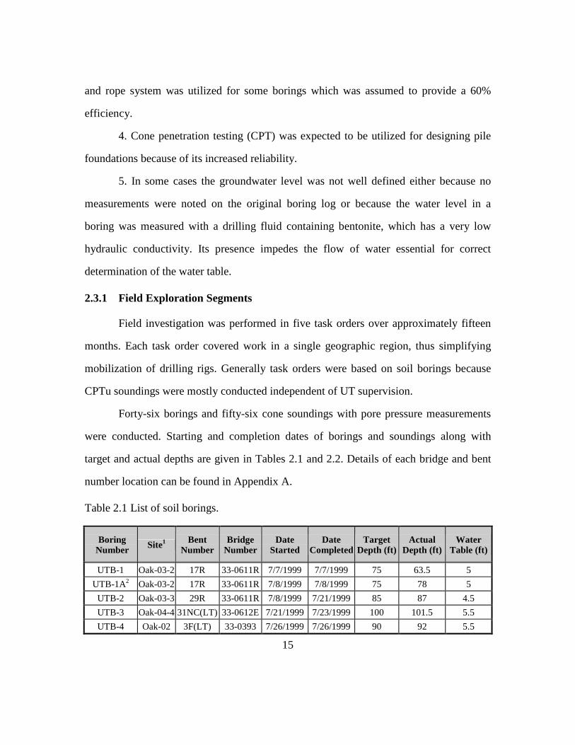
Table 2.1 List of soil borings. ........................................................................................... 15

Table 2.2 Cone Penetration Test (CPT) soundings........................................................... 17

Table 2.3 Laboratory tests and applicable standards. ....................................................... 23

Table 2.4 Summary of completed laboratory tests. .......................................................... 25

Table 2.5 Summary of UU compression tests conducted to investigate the effects of

trimming. ..................................................................................................... 31

Table 3.1 Pile Young’s modulus values applied for analyses. ......................................... 51

Table 3.2 Typical elastic constants of various soils (HB-17: AASHTO Standard

Specifications for Highway Bridges, 17th ed., 2002). ................................ 52

Table 4.1 Summary of pile load tests used in analyzing clayey profiles.......................... 82

Table 4.2 Details of pile load tests with clayey profiles (N = 26). ...................................82

Table 4.3 Summary list of pile load tests analyzed (sandy soils). .................................... 83

Table 4.4 List of pile load tests in sandy profiles (N = 34). ............................................. 84

Table 4.5 Summary list of pile load tests driven into mixed profiles. .............................. 85

Table 4.6 Details of piles founded in mixed soils (N = 68).............................................. 85

Table 5.1 Correlations of Young’s modulus with undrained shear strength, cu. ............ 103

Table 5.2 The statistics of displacement ratio (sc/sm) (N = 26)....................................... 107

Table 5.3 Ranking of correlations based on displacement ratio (sc/sm). ......................... 108

Table 5.4 The statistics for displacement differences (sc-sm) (inch) (N = 26). ............... 109

Table 5.5 Comparison of predicted and measured displacements for outliers. .............. 111

Table 5.6 Details of pile load tests that have been investigated further. ........................ 112

Table 5.7 Range of parameters for all pile load tests in clay compared to those for

outliers. ...................................................................................................... 113

Table 5.8 Correlations for Young’s modulus, Es with SPT blow count (N in bpf). ....... 116

Table 5.9 Mean and standard deviation for correlations (N = 34).................................. 119

xvii

Table 5.10 Rankings corresponding to each correlation.................................................120

Table 5.11 The statistics of displacement difference (sc-sm) for comparison with

correlations in cohesionless soils (N = 34)................................................ 121

Table 5.12 Displacement ratio and difference for outliers. ............................................122

Table 5.13 Properties and soil layering for outlying pile load tests................................ 123

Table 5.14 Range of parameters for all pile load tests in sand versus that for outliers. . 127

Table 5.15 Mean and standard deviation of displacement ratio (sc/sm) for correlations. 134

Table 5.16 Rankings for correlations based on the statistics of sc/sm. ............................ 135

Table 5.17 Summary of the mean and standard deviation for displacement differences (all

in inches). .................................................................................................. 136

Table 5.18 The statistics for the displacement ratios (sc/sm) in cohesive soils. .............. 138

Table 5.19 Mean and standard deviation of displacement differences (sc-sm)................ 138

Table 5.20 Mean and standard deviation of the displacement ratio for predictive methods

in cohesionless soils. ................................................................................. 139

Table 5.21 The statistics of displacement difference (sc-sm) for predictive methods in

cohesionless soils. ..................................................................................... 139

Table 5.22 Statistics of displacement ratio (sc/sm) for predictions in mixed profiles. .... 141

Table 5.23 Summary of mean and standard deviation for displacement differences of

predictions with measurements. ................................................................ 141

Table 6.1 Summary statistics for (sc/sm) and (sc-sm) employing the proposed method

(N=26). ...................................................................................................... 146

Table 6.2 Statistical values for displacement ratios and differences in cohesionless soils

(N=34). ...................................................................................................... 155

Table 6.3 Statistics for settlement ratio (sc/sm) and displacement difference (sc-sm)

(N=83). ...................................................................................................... 161

Table 7.1 Multiplication factors at loading increments (†K1 = Es/cu). ............................ 166

Table 7.2 Values for logarithmic fitting conducted for piles in cohesionless soils. ....... 167

xviii

Table 7.3 Statistics for settlement ratio (sc/sm) and displacement difference (sc-sm)

(N=83). ...................................................................................................... 168

xix

List of Figures Figure 2.1 Sites in Northern California. ....................................................................... 10

Figure 2.2 Sites in Southern California. ....................................................................... 10

Figure 2.3 Trailer-mounted drill rig in operation. ........................................................ 20

Figure 2.4 a) Triaxial sample cutting lathe and miter box, b) Consolidation sample

cutter............................................................................................................ 24

Figure 2.5 Comparison of undrained shear strength values for trimmed versus

untrimmed specimens.................................................................................. 29

Figure 2.6 Relative error for the effect of trimming on UU test results. ...................... 30

Figure 2.7 Changes in water content of trimmed and untrimmed samples. ................. 30

Figure 2.8 The effect of water content on undrained shear strength. ........................... 30

Figure 3.1 a) Displacements and b) loads for a pile in compression (i and j refer to soil

elements). .................................................................................................... 35

Figure 3.2 Geometry and assumptions for Mindlin’s equations (Mindlin, 1936; Poulos

and Davis, 1974). ........................................................................................ 37

Figure 3.3 Shear stress distribution along the side of pile segments. ........................... 41

Figure 3.4 Problem definition by Lee et al. (1987) a) Axially loaded pile in a layered

soil, b) Extended soil layers, c) fictitious pile. ............................................ 43

Figure 3.5 Mirror-image approach for a pile on a rigid base........................................ 47

Figure 3.6 Various definitions of elastic of elastic modulus: Ei: Initial tangent modulus;

Es: Secant modulus; Et: Tangent modulus (defined at a given stress level).53

Figure 3.7 A schematic for the normalized shear modulus – shear strain relationship.55

Figure 3.8 Displacements with varying Young’s modulus and Poisson’s ratio. .......... 56

Figure 3.9 An example for the effect of varying ultimate capacity on the load-

displacement curve. ..................................................................................... 59

Figure 3.10 Conceptual variation of shear modulus with strain level under static

monotonic loading; relevance to in-situ tests (Mayne et al., 2001). (PMT:

pressuremeter; DMT: dilatometer). ............................................................. 61

xx

Figure 3.11 Strain dependence of measurement and analysis of soil properties (Yoshida

and Iai, 1998)............................................................................................... 61

Figure 3.12 A comparison of typical strains applied in laboratory tests versus in-situ

strains around structures (Clayton et al., 1995)........................................... 63

Figure 3.13 Parts and pore pressure sensors of a piezocone penetrometer (CPTU)....... 66

Figure 3.14 Example of a pressuremeter test result (Baguelin et al., 1978)................... 69

Figure 4.1 View of the pre-processing interface for Tapile program. .......................... 90

Figure 4.2 Tapile final screen in command window after execution............................ 91

Figure 4.3 An example of the collected pile load test data in cohesive soil................. 92

Figure 4.4 Flow chart depicting the steps in Tapile analyses (adapted from Poulos,

1979)............................................................................................................ 93

Figure 4.5 Failure load determination (pile weight not considered): a) peak applied

load corresponding to pile capacity in a tension test, b) failure load for a

prematurely terminated pile load test in compression................................. 94

Figure 4.6 Load-displacement envelope....................................................................... 95

Figure 5.1 The magnitude of measured displacements, sm. ........................................ 102

Figure 5.2 Measured displacements over pile diameter. ............................................ 102

Figure 5.3 Young’s modulus correlations with undrained shear strength. ................. 104

Figure 5.4 Difference between calculated pile capacities: Davisson (167 kips) versus

peak applied load (173 kips). .................................................................... 105

Figure 5.5 Comparison of measured and predicted displacements. ........................... 106

Figure 5.6 Comparison of correlations based on mean and standard deviation of

displacement ratio (sc/sm). ......................................................................... 107


displacement differences (sc-sm) (both in inches)...................................... 110

Figure 5.8 Pile diameter versus displacement ratio for outliers. ................................ 113

Figure 5.9 The magnitude of measured displacements for load ratios up to a half. ... 114

xxi

Figure 5.10 Measured displacements over pile diameter for piles in cohesionless

soils............................................................................................................ 115

Figure 5.11 Correlations of SPT blow count with Young’s modulus of soil. .............. 117

Figure 5.12 Measured and predicted displacements for piles in sandy soils................ 118


displacement ratio (sc/sm). ......................................................................... 119

Figure 5.14 Comparison of predictions based on mean and standard deviation of

displacement difference (sc-sm). ................................................................ 121

Figure 5.15 Pile diameter and displacement ratio for all tests and outliers. ................. 126

Figure 5.16 The pile stiffness and displacement ratio for all tests and outliers............ 127

Figure 5.17 Magnitudes of measured displacements.................................................... 129

Figure 5.18 Absolute value of measured displacements, sm, divided by pile

diameter, D. ............................................................................................... 130

Figure 5.19 Comparison of displacements for piles driven into mixed profiles

(N = 83). .................................................................................................... 131

Figure 5.20 Comparison of displacements predicted using Frank’s correlation. ......... 132

Figure 5.21 Predictions utilizing the elastic column approach in mixed profiles......... 133

Figure 6.1 Young’s modulus versus undrained shear strength for each load ratio

(N=26). ...................................................................................................... 144

Figure 6.2 Change of Young’s modulus with undrained shear strength and fitted

correlations. ............................................................................................... 145

Figure 6.3 Calculated and measured displacements using suggested correlations..... 146

Figure 6.4 Comparison of proposed Es correlations with others from literature. ....... 147

Figure 6.5 Suggested correlations and data for concrete piles (N=6)......................... 148

Figure 6.6 Suggested correlations and available data for closed-ended pipe piles

(N=3). ........................................................................................................ 148

xxii

Figure 6.7 Calculated Young’s moduli from pile load tests and suggested correlations

for open-ended pipe piles (N=17). ............................................................ 149

Figure 6.8 Variations of Young’s modulus with SPT blow count (N=34)................. 150

Figure 6.9 Young’s modulus versus blow count in logarithmic axes given along with

fitted curves (N=31). .................................................................................151

Figure 6.10 The effect of varying displacements on the values of Young’s modulus. 153

Figure 6.11 Comparison of fitted curves to Young’s modulus versus blow count results

at each load ratio. ...................................................................................... 154

Figure 6.12 Fitted curves in relation to other recommended correlations for cohesionless

soils............................................................................................................ 155

Figure 6.13 Displacements calculated for piles in cohesionless soils using correlations

derived from Caltrans database. ................................................................ 156

Figure 6.14 Values of Young’s modulus obtained for the closed-ended pipe pile

(N=1). ........................................................................................................ 157

Figure 6.15 Calculated Young’s modulus for concrete-filled pipe piles (N=2). .......... 157

Figure 6.16 Young’s modulus values calculated from H-piles in Caltrans pile load tests

(N=4). ........................................................................................................ 158

Figure 6.17 Variation of Es and N for concrete piles (N=6)......................................... 158

Figure 6.18 Young’s modulus versus SPT N for open-ended pipe piles (N=18)......... 159

Figure 6.19 Predicted and measured displacements of piles in mixed profiles

(N=83). ...................................................................................................... 160

1

Chapter 1: Introduction

1.1 MOTIVATION

Limits must be placed on displacements of structures, especially differential

displacements, to minimize damage. These limits can vary based on the type and

importance of the structure. For example, the limit for heavy multi-storied structures is

much less than that for a steel-framed warehouse. Drilled or driven piles are generally

utilized in cases where shallow foundations do not provide a satisfactory outcome.

However, once the decision for piles is made, the typical design approach is to ensure

that the estimated capacity is greater than the expected loading multiplied by a safety

factor to include uncertainties. Such an approach implicitly assumes that the

displacements will remain within tolerable amounts. A recent trend considers

serviceability limits to apply the LRFD (load and resistance factor design) approach

(Barker et al., 1991; CFEM, 2006; Eurocode 7, 1997; NCHRP Report No. 507, 2004).

Nevertheless, limitations of budget, time, available resources in terms of personnel and

computing, and the provided site/soil information are all reasons for overlooking pile

displacement.

Usually the displacements of individual piles are small and most are complete

during or shortly after the loads are applied without adverse effects to the structures.

Nevertheless, displacements may be an important factor for various conditions; for

example when long and compressible piles are considered, when piles are driven in dense

cohesionless soils and large loads are involved, when static loads represent a large

fraction of the total load and soil is susceptible to increased displacements with time, or

when live loads are applied and removed cyclically due to wind or wave. Stricter

2

structural requirements for some facilities may also call for the evaluation of

displacements.

1.2 PILE LOAD DATABASE

Axial pile load tests are conducted to have a better understanding of pile capacity

and load-displacement behavior, reducing the uncertainty involved with the design and

implementation. The costs of performing a pile load test may lead to savings due to the

reduced safety factors and increased reliability of the results. However, it may not be

feasible to carry out tests during the initial phases of a design or if the piles are proposed

at a location where the designers already have a significant amount of experience and

knowledge. Pile load test databases combine such collected experience at different

locations in a convenient manner. Databases can be beneficially utilized to find piles and

site conditions similar as to type, length, diameter, and soil layering as to those that are

under consideration.

A database comprised of axial pile load tests conducted at multiple locations

throughout California has been employed to predict load-displacement behavior. The pile

load tests have been provided by the California Department of Transportation (Caltrans).

Additional in-situ testing involving cone soundings and standard penetration tests, and

soil borings have been completed at or near the location of the pile load tests to

supplement the furnished information. Various laboratory tests conducted on the soil

samples collected from borings are also included to augment the parameters for the

evaluation and development of predictive methods. The author supervised the fieldwork

and actively participated in all phases of laboratory testing.

The database initially contained 337 pile load tests on 239 piles at eighty-three

Californian bridges and abutments. However, the database used for this dissertation

3

(FinalCT.dat dated May 29, 2005) has been reduced to 143 pile load tests due to various

complications and restrictions with the initial information. All of the tested piles were

driven into the ground. Measurements of displacements and loads were made only at the

top of the pile.

Although the data incorporated into the study were based on pile load tests

conducted in California, this dissertation is expected to have broader implications to

predict pile displacements in other regions because multiple types of soils and piles are

considered.

1.3 RESEARCH APPROACH

Prediction of the response of a single friction pile to axial loading involves an

analysis of soil-pile interaction. Under ideal circumstances, the design engineer would

like to predict the entire load-displacement curve, along with the rate of load transfer

from the pile to the soil as a function of depth. Practically, though, failure load is

estimated along with a prediction of the displacements under working loads, which is

defined as a factor of safety between two to three applied to the failure load. Practical

rules of thumb have been suggested for estimating displacements for such cases based on

pile diameter (Vesic, 1970; Briaud and Tucker, 1985; Frank, 1985, 1995). However, a

more accurate analytical approach should undoubtedly involve other relevant parameters

such as pile length and soil layering.

For determining displacements, the empirical elastic or load transfer (t-z) methods

are usually favored over more sophisticated, yet complicated and costly approaches such

as finite elements methods. They are simpler to set-up and can rapidly be conducted with

the aid of computer codes. Although potentially more universal, sophisticated and

accurate, finite element or boundary element methods have not been widely accepted as

4

part of routine geotechnical engineering practice for pile design. Costs involved due to

the complexity of models and the difficulty of obtaining relevant parameters can be listed

as reasons for the lack of implementation. Some suggested soil models require a

significant number of parameters (up to fifteen) to be determined with specialized

laboratory and/or field testing (Whittle, 1993; Barbour and Krahn, 2004).

In this dissertation, the displacements of axially loaded single piles are explored

using a modification of Mindlin’s solution (1936) based on elasticity, which provides a

solution to predict displacements within a semi-infinite soil mass induced by a vertical

load. Changes are made to the original solution to account for:

- varying soil conditions and layering (Poulos and Davis, 1968; Poulos,

1979),

- assumptions of stresses and displacements acting on the soil-pile

interface (D’Appolonia and Romualdi, 1963; Salas, 1965; and Poulos

and Davis, 1968), and

- residual stresses (Poulos; 1987).

Young’s modulus or modulus of elasticity, Es, and Poisson’s ratio, νs, of the soil

along the periphery and below the tip of a pile are the two parameters that influence the

predictions in this approach. However, the effect of Young’s modulus on the predicted

displacements is much more pronounced than Poisson’s ratio; therefore, the focus in this

study is towards establishing an approach to determine appropriate values of Es.

Many researchers have suggested Young’s modulus correlations with a multitude

of parameters. Most of the correlations involve simple, readily available laboratory

and/or in-situ information. These Young’s modulus correlations can be utilized to predict

displacements with the elastic method. A few of these relationships are evaluated in this

5

dissertation to investigate the accuracy of the predictions when compared to the

measurements from pile load tests within the compiled database. While the laboratory

triaxial undrained shear strength, cu, is employed for cohesive soils, the standard

penetration test blow count, N, is used for cohesionless soils.

In addition to evaluating existing correlations, the same pile load test data are

utilized to obtain back-calculated values of Young’s moduli in order to improve the

predictions of load-displacement behavior. The measured displacements at loads of a

third, a half, and two-thirds of the failure load (or determined pile capacity) are iteratively

matched by a trial-and-error process. Separate Young’s modulus correlations are obtained

for cohesive and cohesionless soils. The correlation factors thus derived are then used to

predict the displacements of piles driven in mixed profiles. The displacements at

increasing load increments can be used to construct a complete load-settlement curve.

1.4 DISSERTATION OUTLINE

This dissertation contains seven chapters and two appendices. An outline for each

chapter is given below.

The database used for analyses in this dissertation is described in Chapter 2, with

an emphasis given to the field and laboratory testing conducted in support of the

information provided by the California Department of Transportation.

The theory behind the elastic method and its modifications suggested by other

researchers to better simulate load-displacement behavior of single axially loaded piles

are described in Chapter 3.

In Chapter 4, the database is broken into three main classifications according to

the type of soil in which the piles are founded. Definitions are given for cohesive,

cohesionless and mixed soil profiles. Relevant information regarding the pile load test

6

database is summarized in tables. The graphical and statistical evaluations in the

following chapters are explained.

In Chapter 5, analyses of pile load tests based on recommended correlations

obtained from the literature are shown. Results are compared to the measurements from

actual pile load tests. Suggested correlations are ranked in terms of the ratio of calculated

to measured displacements (“displacement ratio”) as well as the difference between the

two displacement values (“displacement difference”).

Attempts to obtain improved correlations for Young’s modulus with widely

available parameters for cohesive and cohesionless soils are described and evaluated in

Chapter 6. The outcome is placed in context with correlations employed in the previous

chapter.

Conclusions of this research, shortcomings and recommendations for extending

the findings are given in the last chapter.

Appendix A contains a listing of site names, bridge numbers, pile load test

numbers, and other descriptive terms used in tables in Chapters 2 and 4.

Correlations collected from literature relating a wide range of parameters to

Young’s modulus are given in Appendix B.

Appendix C includes an example of the input and output files used in estimating

displacements with Tapile computer code.

7

Chapter 2: Pile Load Database

2.1 INTRODUCTION

An axial pile load test database from locations throughout California was

compiled and utilized as part of this dissertation. The information was furnished by the

California Department of Transportation. Fifty-six cone soundings, numerous standard

penetration tests and forty-six soil borings were conducted to supplement the furnished

information. Laboratory tests are also conducted on the soil samples collected from

borings.

In this chapter the establishment of the pile load test database is described along

with various aspects of laboratory and in-situ tests conducted as part of an effort to

increase the available information. Limitations observed in the compiled data are

discussed.

2.2 PILE LOAD DATABASE

Typical California Department of Transportation (Caltrans) practice is to install

driven piles to support structures such as abutments, overpasses, and bridges within the

state. The design of such piles commonly relies on general site investigations providing

sample descriptions along with measures of undrained shear strength for cohesive soils

and standard penetration resistance for cohesionless soils without any further laboratory

and/or in-situ tests. The importance of improved understanding of soil properties and

proficient design approaches to pile foundations were underscored following major

structural failures and financial ramifications of earthquakes in California, such as Loma

Prieta in 1989 and Northridge in 1994. The retrofit efforts following these earthquakes

8

have resulted in “overdesign” of foundations, i.e., an approach that is conservative and

costly (DiMillio, 1999).

Since 1957, Caltrans has conducted a large number of pile load tests

(approximately 450 by July 1994 at a cost reaching $30,000 per test, Liebich 2003) as

part of an intense effort to estimate the capacity of their piles. Unfortunately, the

accumulated experience has not yet translated into improved design approaches.

Typically basic general site investigations were conducted as part of designing piles for

Caltrans. Common pile design methods could not be used because generally no

laboratory testing was conducted. The pile load tests were mainly conducted to verify

capacity and were not an integral part of a standard pile design. Piles were often driven

essentially to refusal. Pile design estimates of load capacity were commonly compared to

those obtained from dynamic formulas (Engineering News, Hiley, etc.) based on pile

driving records. Furthermore, the capacity was determined using a half-inch failure

criterion, in which the load measured at half an inch of displacement is considered as the

pile capacity based on recommendations of structural engineers. Results from load tests

on instrumented piles found in the literature indicate that side and tip capacities develop

at different displacements. Shaft capacity reaches its peak value at a lower displacement

than the tip capacity. Thus, a constant displacement value having a constant value as a

failure criterion may lead to uneconomical designs if sufficient displacement is not

allowed to mobilize tip capacity. Despite these shortcomings, a half-inch displacement

continues to be Caltrans’ preference for defining pile capacity and remains as a critical

parameter for design (Caltrans California Foundation Manual, 1997).

In the summer of 1998, Caltrans funded a project at The University of Texas at

Austin entitled “Improvement of Caltrans Pile Design Methods through Synthesis of

9

Load Test Results” to evaluate years of accumulated pile load test data and ultimately to

develop updated design methodologies. This dissertation focuses on the load-

displacement behavior of piles based on the information supplied by Caltrans and on

additional testing conducted in the field and in the laboratory as part of this project.

Initially, Caltrans provided an archive of pile test reports that contained

measurements of pile head load-displacements along with site characterization

information, which were entered in the “Geotechnical Measurements Database” (GMD)

established by Brown (2001). The GMD includes 319 static load tests on 227 untapered

(no changes in the cross-section) driven piles in 161 pile groups at 75 bridge locations

throughout California. Additional laboratory and field investigations were conducted,

which likewise contributed to the GMD. Further details of the GMD can be found in

Brown (2001). Two tables coupling the bridge numbers, site names and locations, load

test numbers and other descriptive terms for all of the pile load tests are provided in

Appendix A. Designation from these tables was also used to provide details for project

borings and soundings (Tables 2.1 and 2.2). A general overview of pile load test locations

sorted by counties is shown in Figures 2.1 and 2.2. The majority of the Caltrans data is

concentrated in areas near California’s largest metropolitan centers: Los Angeles, San

Diego and the Bay Area. A few other tests were conducted at remote bridge locations.

10

Figure 2.1 Sites in Northern California.

Figure 2.2 Sites in Southern California.

11

At the beginning of the project, the aim was to enter essentially all available data

into the GMD and then to utilize those tests which were deemed useful in developing

design methods. In some cases, inadequacies in data were not apparent until analyses

were attempted. Since 2001, analysis and checking of the interpreted soil profiles

included in the GMD have resulted in modifications (Olson, 2005). The main reasons for

such changes are the reevaluation of pile load test reports, additional field/laboratory

investigations provided by Caltrans, incorporation of pile driving records into the site

characterization, and an increased emphasis on soil borings that were conducted as part of

this project.

Therefore, a database called FinalCT (Olson, 2005) was created as a text file,

which is similar to that established for the American Petroleum Institute by Olson and

Dennis (1982). The number of load tests in FinalCT was reduced to 143 from 337 in the

GMD.

In this dissertation, the load-displacement behavior is investigated utilizing the

pile load tests listed in the FinalCT database.

2.2.2 Limitations of Both Pile Load Test Databases

Despite frequent revisions, neither database can be considered ideal. Obviously a

database is only as good as the data included in it. In some cases, the locations of the pile

load tests were not readily accessible due to restrictions from owners, and the presence of

utilities that restricted access. Among the other most evident limitations of both databases

are the following:

1. There is no instrumentation along the length of any pile; i.e., only pile-head

load and displacement measurements are available. Therefore, the distributions of loads

12

and displacements along the sides and on the tip have not been properly assessed. They

may at best be estimated from previous experience.

2. Some of the pile load tests were not carried to failure or had very few data

points. The goal in most of these cases was to evaluate the performance of a pile within

working loads, but unplanned situations such as equipment malfunction, failure of

support piles, etc., also occurred. Piles tested within working loads may be useful in

analyzing displacements up to that load but they do not provide pile capacities.

3. Setup time (the time between driving the pile into the ground and load testing)

is either not known or was not sufficient for some pile load tests (less than a week in

clayey profiles and a day for piles in coarser materials). Setup time may increase the load

carrying capacity of piles due to pore-pressure changes or stress distributions in the soil.

4. In some of the older tests, there is no clear indication of the loading direction.

However, in most such cases, an estimate has been made based on further evaluation of

the load test report.

5. When a pile was tested in both compression and tension, one following the

other, the properties of the soil surrounding the pile might have been affected by the first

load test and thus the second load test might not produce capacities that would have been

achieved in the absence of a previous load test.

6. It was not always clearly stated whether steel pipe piles were open-ended or

closed-ended. The size of the cover plate might be missing even if there was a note that

the steel pipe pile was closed-ended.

7. Soil borings were sometimes not close to the pile because of restricted site

access. In other cases, it was difficult to determine the precise location and top

13

elevation of a test pile due to site regrading. This may have significantly affected soil

characterization, considering the heterogeneous nature of soil properties.

8. The soil profiles and SPT blow counts were estimated from pile driving records

if there were no borings at or near the location of a pile load test (FinalCT only). Notes

were made to indicate which blow counts were estimated.

9. Most of the piles are in interstratified profiles, which complicate analyses and

make it more difficult to separate pile behavior in a specific material within the strata.

10. All of the piles in this study were used for supporting bridges and all were in

significant earthquake zones. These conditions restricted the type and size of the piles.

Predominantly, steel pipe piles were used.

11. The project boring and sounding elevations do not necessarily correspond to

the tested pile elevations. Many of the piles were driven at the bottom of excavations

below the surface elevation where soil explorations were made.

12. For storage purposes, original Caltrans soil boring and sounding logs were

reduced greatly in size by Caltrans through photocopying, which made them difficult to

read. In older reports, the quality of the report reproduction was low.

In-spite of the limitations listed above, any approach based on the established

databases is expected to improve future Caltrans’ design methods for foundations

constructed in soil profiles typically encountered in California. It can also reduce

construction costs by eliminating overly-conservative designs and provide design

engineers with site-specific information. Additionally, a database provides a basis for any

future improvements of aspects not considered within the University of Texas at Austin

(UT) project.

14

The Federal Highway Administration (FHWA) has pooled pile load tests from a

multitude of state highway departments and established a pile load test database

containing a broad range of information. FHWA has recently updated its deep

foundations design guidelines and manuals, which are widely used (Design and

Construction of Driven Pile Foundations Reference Manual – Volumes I and II, 2006).

Caltrans, under the umbrella of FHWA, similarly sponsored the project at UT with the

aim of being a part of the occurring changes. Results from this dissertation are aimed

towards providing additional insight into the load-displacement aspect of designing pile

foundations.

2.3 FIELD INVESTIGATION

Additional borings and in-situ tests beyond those which existed in Caltrans files

were conducted at selected sites where subsurface information was deemed inadequate.

The main reasons for this evaluation are the following:

1. For a pile design relying on empirical correlations, it is reasonable that all

relevant parameters be obtained in a consistent manner to avoid any uncertainties

regarding the test method or equipment. Relatively undisturbed soil samples were

obtained to re-evaluate visual classification and perform laboratory tests. This is the most

important reason for conducting additional soil borings.

2. In some cases the original Caltrans soil borings were too far from the site of the

load test to characterize the subsurface conditions adequately.

3. Standard penetration test (SPT) hammers vary in the energy that they transfer

to the rods resulting in uncertainty in terms of the blow counts being measured. A

calibrated hammer with an 80% efficiency was used for most of the borings. A cathead

15

and rope system was utilized for some borings which was assumed to provide a 60%

efficiency.

4. Cone penetration testing (CPT) was expected to be utilized for designing pile

foundations because of its increased reliability.

5. In some cases the groundwater level was not well defined either because no

measurements were noted on the original boring log or because the water level in a

boring was measured with a drilling fluid containing bentonite, which has a very low

hydraulic conductivity. Its presence impedes the flow of water essential for correct

determination of the water table.

2.3.1 Field Exploration Segments

Field investigation was performed in five task orders over approximately fifteen

months. Each task order covered work in a single geographic region, thus simplifying

mobilization of drilling rigs. Generally task orders were based on soil borings because

CPTu soundings were mostly conducted independent of UT supervision.

Forty-six borings and fifty-six cone soundings with pore pressure measurements

were conducted. Starting and completion dates of borings and soundings along with

target and actual depths are given in Tables 2.1 and 2.2. Details of each bridge and bent

number location can be found in Appendix A.

Table 2.1 List of soil borings.

Boring Number Site1 Bent

Number Bridge

Number Date

Started Date

Completed Target

Depth (ft) Actual

Depth (ft) Water

Table (ft)

UTB-1 Oak-03-2 17R 33-0611R 7/7/1999 7/7/1999 75 63.5 5

UTB-1A2 Oak-03-2 17R 33-0611R 7/8/1999 7/8/1999 75 78 5

UTB-2 Oak-03-3 29R 33-0611R 7/8/1999 7/21/1999 85 87 4.5

UTB-3 Oak-04-4 31NC(LT) 33-0612E 7/21/1999 7/23/1999 100 101.5 5.5

UTB-4 Oak-02 3F(LT) 33-0393 7/26/1999 7/26/1999 90 92 5.5

16


Number Bridge

Number Date

Started Date

Completed Target

Depth (ft) Actual

Depth (ft) Water

Table (ft)

UTB-5 Oak-04-3 27NC(RT) 33-0612E 7/27/1999 7/28/1999 115 115.5 7.5

UTB-6 Oak-04-1 10NCI 33-0612E 7/28/1999 7/29/1999 110 110 6

UTB-7 Oak-01-1 E28L 33-0025 7/30/1999 7/30/1999 60 62 4

UTB-8 Oak-04-2 17NC1 33-0612E 8/23/1999 8/25/1999 110 112.5 6

UTB-9 Oak-05-3 Site 3 I880 IPTP 8/25/1999 8/27/1999 115 119 5

UTB-10 Oak-05-1 Site 1 I880 IPTP 8/30/1999 8/30/1999 45 46.5 14 UTB-11 Oak-05-2 Site 2 I880 IPTP 8/30/1999 8/30/1999 65 22 4.5

UTB-11A Oak-05-2 Site 2 I880 IPTP 8/31/1999 8/31/1999 65 65.5 4.5 UTB-12 Oak-05-4 Site 4 I880 IPTP 9/1/1999 9/2/1999 85 87.5 4

UTB-13 SJ-01 4 37-0011 9/8/1999 9/9/1999 75 77 15

UTB-14 SJ-02-2 GD-2, 6 37-0270H 9/10/1999 9/13/1999 60 61.5 25

UTB-15 SJ-03-3 6L-2 37-0279L 9/14/1999 9/14/1999 75 77 14.5

UTB-16 SJ-02-3 GD-2, 14 37-0270H 9/15/1999 9/15/1999 80 83.5 20.5 UTB-17 SJ-04 DC-4, 8 37-0353 9/16/1999 9/16/1999 85 89 7.5 UTB-18 SF-03-3 Site C 34-0088 3/27/2000 3/27/2000 75 75.5 N/A UTB-19 SF-03-4 Site D 34-0088 3/28/2000 3/28/2000 70 70 11.5

UTB-20 SF-03-6 Site F 34-0088 3/29/2000 3/29/2000 80 80 9

UTB-21 SF-03-5 Site E 34-0088 3/30/2000 3/31/2000 105 106.5 6.5

UTB-22 SF-03-7 Site G 34-0088 3/31/2000 4/3/2000 90 90.5 7.5

UTB-23 Oak-04-4 31NC(LT) 33-0612E 4/4/2000 4/4/2000 100 102 5

UTB-24 Oak-04-2 17 NC1 33-0612E 4/5/2000 4/5/2000 110 7.25 2.5

UTB-24A Oak-04-2 17NC1 33-0612E 4/5/2000 4/5/2000 110 110 2.5

UTB-25 LA-03 5 53-1181S 5/31/2000 5/31/2000 50 50 18

UTB-26 LA-01-1 10 53-0527L 6/1/2000 6/1/2000 60 60 39.5

UTB-27 LA-13-1 2 53-2733 6/2/2000 6/2/2000 45 45 26

UTB-28 LA-14 5 53-2791S 6/3/2000 6/3/2000 70 70 22.5

UTB-29 LA-09 21 Foot. A 53-1851 6/5/2000 6/5/2000 50 50 20

UTB-30 LA-22 8 55-0794F 6/6/2000 6/6/2000 65 65 28

UTB-31 LA-20 4 55-0682F 6/7/2000 6/7/2000 65 65 N/A

UTB-32 LA-17 6 55-0642 6/8/2000 6/8/2000 70 70 N/A

UTB-33 LA-21-2 16 55-689E 6/8/2000 6/8/2000 70 70 N/A

UTB-34 LA-15 2 55-0422G 6/13/2000 6/13/2000 60 60 17

UTB-35 LA-02 5 53-0114 6/14/2000 6/14/2000 60 60 42

UTB-36 SD-07-2 2L 57-1017R/L 6/15/2000 6/15/2000 40 40 15.5

UTB-37 SD-07-1 Abutm. 7R 57-1017R/L 6/15/2000 6/15/2000 30 30 15.5

17


Number Bridge

Number Date

Started Date

Completed Target

Depth (ft) Actual

Depth (ft) Water

Table (ft)

UTB-38 SD-08-2 Site 2 I-5/I-8 IPTP 6/16/2000 6/16/2000 120 118.5 23

UTB-39 SD-03 5 57-0783F 6/17/2000 6/17/2000 60 60 19

UTB-40 Oak-05-2 Site 2 I880 IPTP 9/12/2000 9/12/2000 60 61.5 4

UTB-41 Oak-05-4 Site 4 I880 IPTP 9/13/2000 9/13/2000 90 92.5 4

UTB-42 SM-02 8B 35-0284 9/14/2000 9/15/2000 115 115 12.5

UTB-43 CC-02 5L 28-0056L 9/18/2000 9/18/2000 75 75 8.5

UTB-44 Mon-03 Test Group

44-0216R/L 9/19/2000 9/20/2000 140 141.5 8

UTB-45 Son-01 3 20-0172 9/21/2000 9/22/2000 60 60.5 10

UTB-46 Son-02 Abutm. 2R 20-0251R 9/22/2000 9/23/2000 60 60 9 1 The corresponding load test numbers, cities and counties are given in Appendix A. 2 A subsequent boring or sounding attempt was made at the same location due to an obstruction at some depth or a difficulty in reaching target depth.

Table 2.2 Cone Penetration Test (CPT) soundings.

CPT Number Site Bent

Number Bridge

Number Date Target Depth

(ft)

Actual Depth

(ft)

Depth Ratio (%)

Predrill Depth

(ft)

UTC-1 Oak-03-1 13L 33-0611L 7/8/1999 90 68 76 10

UTC-1A Oak-03-1 13L 33-0611L 7/8/1999 90 69 77 5

UTC-2 Oak-03-2 17R 33-0611R 7/9/1999 75 66 88 5.5

UTC-3 Oak-03-3 29R 33-0611R 7/9/1999 85 85 100 7.5

UTC-4 Oak-02 3F(LT) 33-0393 7/21/1999 90 90 100 0

UTC-5 Oak-04-4 31NC(LT) 33-0612E 7/23/1999 100 100 100 9

UTC-6 Oak-04-3 27NC(RT) 33-0612E 7/22/1999 115 115 100 0

UTC-7 Oak-04-2 17NCI 33-0612E 7/22/1999 110 110 100 0

UTC-8 Oak-01-1 E28L 33-0025 7/26/1999 60 60 100 10

UTC-9 Oak-01-2 E31R 33-0025 7/22/1999 65 65 100 0

UTC-10 Oak-05-1 Site 1 I-880 IPTP 7/23/1999 45 34 76 4.5

UTC-11 Oak-04-1 10NCI 33-0612E 7/23/1999 110 110 100 8

UTC-12 Oak-05-3 Site 3 I-880 IPTP 7/26/1999 115 115 100 0

18


Number Bridge


(ft)

Actual Depth

(ft)

Depth Ratio (%)

Predrill Depth

(ft)

UTC-13 Oak-05-2 Site 2 I-880 IPTP 9/14/1999 60 42.5 71 16


UTC-15 SJ-02-2 GD-2, 6 37-0270H 9/8/1999 60 55 92 6

UTC-16 SJ-02-4 GD-4, 3 37-0270H 9/8/1999 60 60 100 5.5

UTC-17 SJ-02-3 GD-2, 14 37-0270H 9/9/1999 80 80 100 7

UTC-18 SJ-02-5 GD-4, 11 37-0270H 9/9/1999 60 60 100 5.5

UTC-20 SJ-01 4 37-0011 9/13/1999 75 75 100 7

UTC-21 SJ-03-1 2L-2 37-0279L 9/9/1999 75 75 100 5

UTC-22 SJ-03-3 6L-2 37-0279L 9/13/1999 70 70 100 5

UTC-23 SJ-03-2 3R-2 37-0279R 9/9/1999 70 70 100 0

UTC-24 SJ-04 DC-4, 8 37-0353 9/13/1999 85 85 100 6

UTC-25 SF-03-3 Site C 34-0088 3/27/2000 75 50.2 67 25

UTC-25A SF-03-3 Site C 34-0088 3/27/2000 75 15.6 21 0

UTC-26 SF-03-5 Site E 34-0088 3/30/2000 105 89.2 85 3.5

UTC-26A SF-03-5 Site E 34-0088 3/30/2000 105 120 114 3.5

UTC-27 LA-01-1 10 53-0527L 6/13/2000 55 35 64 0

UTC-28 LA-14 5 53-2791S 6/13/2000 70 40 57 0

UTC-29 LA-09 21 Foot. A 53-1851 6/13/2000 50 36.3 73 0

UTC-30 LA-02 5 53-0114 6/14/2000 60 60.5 101 0

UTC-31 LA-13-1 2 53-2733 6/14/2000 45 50.5 112 0

UTC-32 LA-04 6 53-1193S 6/14/2000 60 60.5 101 0

UTC-33 LA-20 4 55-0682F 6/14/2000 65 52.2 80 0

UTC-34 LA-21-2 16 55-689E 6/14/2000 70 70.5 101 0

UTC-35 LA-17 6 55-0642 6/14/2000 70 70.5 101 0

UTC-36 LA-15 2 55-0422G 6/14/2000 60 60.5 101 0

UTC-37 SD-07-2 2L 57-1017R/L 6/15/2000 40 41.3 103 0

UTC-38 SD-07-1 Abutm. 7R 57-1017R/L 6/15/2000 30 35.6 119 0

UTC-39 SD-08-2 Site 2 I-5/I-8 IPTP 6/15/2000 120 11.3 9 0

UTC-40 SD-03 5 57-0783F 6/15/2000 60 57.7 96 0

UTC-41 SF-03-1 Site A 34-0088 5/18/2000 70 40 57 0

UTC-42 SF-03-2 Site B 34-0088 5/18/2000 80 57 71 0

UTC-43 SF-03-7 Site G 34-0088 5/18/2000 90 91 101 0

UTC-44 SF-03-6 Site F 34-0088 5/18/2000 80 52 65 0

UTC-45 SF-03-4 Site D 34-0088 5/19/2000 70 53 76 0

UTC-461 SF-01-8 52R 34-0046 5/19/2000 62.5 0

19


Number Bridge


(ft)

Actual Depth

(ft)

Depth Ratio (%)

Predrill Depth

(ft)


UTC-51B Oak-05-4 Site 4 I-880 IPTP 10/19/2000 85 90 106 0





UTC-561 CC-04 Abutm. 3 28-0292 10/24/2000 75 75 100 0

UTC-59 SF-03-3 Site C 34-0088 3/28/2000 75 50 66 0

UTC-60 SF-03-3 Site C 34-0088 3/28/2000 75 15 21 0 1 The number(s) that follow have not been used.

The first and second field exploration segments were conducted in July, August

and September, 1999, for sites in Oakland and San Jose (borings UTB-1 through UTB-

17). The third field exploration segment (UTB-18 through UTB-24A) was conducted in

March, 2000, after a reconnaissance of San Francisco sites by Caltrans. Unfortunately,

two major San Francisco sites, SF-01 and SF-04, had to be eliminated because of access

problems. In exchange, one large San Francisco site (SF-03) was added. More detailed

plans were drawn up, including scheduling of the third, fourth and fifth field exploration

segments. At this point, funding became available for additional field work. Several sites,

which had been excluded from the original plan because of the presence of dense gravel,

cobbles or boulders were added to the fourth segment (UTB-25 through UTB-39), which

was conducted in May and June, 2000. The fifth field exploration segment (UTB-40

through UTB-46), completed in September, 2000, was the last one at which the author

was on site and in which UT was directly involved.

20

2.3.1.2 Drilling and Sampling Methods

Boreholes were usually drilled with a 5-inch diameter solid-flight auger until

groundwater was reached (Figure 2.3). Casings were set following the determination of

the water table. Drilling was then continued with a 5-inch diameter wet rotary until the

desired borehole depth was reached. An exception to this practice was during the fourth

segment in Southern California, where an NX-type (approximately 3-inch OD) hollow-

stem rod with a drill bit attached was utilized. This is a wet rotary system with rods that

provide a continuous casing throughout the borehole length, and, thereby, help keep

boreholes clean so as to penetrate more easily through sands and gravels. For these cases,

standard penetration tests were conducted through the end of the hollow-stem rod. It was

necessary to pull the rods out before Shelby tube samples could be obtained. Therefore,

the use of these NX-type hollow-stem rods was not desirable for “undisturbed” sampling.

Figure 2.3 Trailer-mounted drill rig in operation.

Undisturbed or standard penetration test (SPT) samples were taken every five feet

starting at a depth of five feet below the ground surface. A standard split-spoon sampler

with a driving shoe inside diameter of 1.375 inches was used without any liners for sands

21

and gravels. Thin-walled tubes (area ratio = 9%) of 30-inch nominal length and 3-inch

nominal diameter were utilized for sampling silts and clays.

Standard penetration tests employed an automatic hammer except those that were

subcontracted in some locations in Northern California, where a falling weight safety

hammer was used. The automatic hammers used in the project were calibrated by the

manufacturer using energy measurements with a pile driving analyzer (PDA). The PDA

utilizes strain gauges and accelerometers to derive the energy transferred from the

hammer to the sampling rods.

2.3.1.3 Water Levels

Water table determination is essential to evaluate the effective stresses at any

depth, which is particularly important information when the design is based on effective

stresses.

Generally, the depth of the water level in the borehole was measured using a

“water level indicator” (an electric sounder which is a calibrated tape measure with an

electrical sensor at the tip that makes an audible sound upon entering water and

completing the circuit; also called “watermeter”). At the beginning of the project and at

some other times when a watermeter was not available, measurements were taken by

lowering a regular tape measure down the borehole. Occasionally the boring failed to

reach the water table or the sides of the borehole collapsed, thus preventing readings.

Water table measurements may be susceptible to errors due to fluctuation from

the drilling operation. A dissipation test during a CPT sounding can provide a better

evaluation of the water table, but requires a longer time to complete. Therefore, a

comparison of water table measurements obtained from drilling and cone soundings was

made at one of the sites (boring UTB-36 and corresponding sounding UTC-37). Drilling

22

and CPTu rigs were operating 14 feet apart at the same time. A water level measurement

was made with the water meter during drilling and with a dissipation test during the

CPTu operation. The watermeter detected water at a depth of 15.7 feet whereas the

dissipation test indicated the water table to be at 18 feet. The ground surface was

essentially horizontal between the two locations.

The writer is not aware of any studies comparing water table measurement in a

borehole as opposed to through a CPT dissipation test. A single measurement is not

sufficient to reach any conclusions as to the accuracy of each method, particularly when

the exact water levels are not known. While a difference of 2.3 feet can be significant for

load tests on shallow foundations, its effect will be less important for piles extending to

deep soil layers.

2.4 LABORATORY TESTING AND RESULTS

Laboratory tests on samples obtained during the field investigation phase were

performed at the University of Texas at Austin or subcontracted to Fugro geotechnical

testing laboratory in Houston, Texas. The testing program was geared towards collecting

data that might be readily obtained by pile-designing engineers. Laboratory testing

included the following: index tests (sieve analysis, Atterberg limits), unconsolidated-

undrained (UU) triaxial compression, and one-dimensional consolidation (oedometer).

Most of the tests on samples from borings UTB-18 through UTB-46 and some of

the remaining Atterberg limit tests and all of the sieve analyses from the first seventeen

borings were performed by the geotechnical testing laboratories of Fugro Consultants in

Houston, TX.

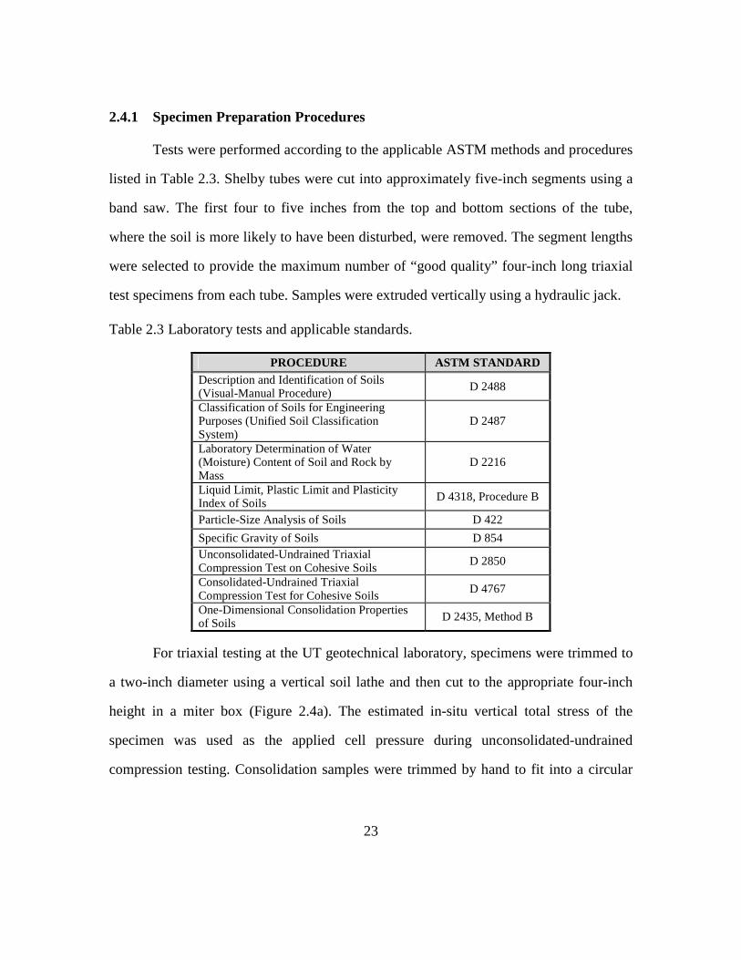
23

2.4.1 Specimen Preparation Procedures

Tests were performed according to the applicable ASTM methods and procedures

listed in Table 2.3. Shelby tubes were cut into approximately five-inch segments using a

band saw. The first four to five inches from the top and bottom sections of the tube,

where the soil is more likely to have been disturbed, were removed. The segment lengths

were selected to provide the maximum number of “good quality” four-inch long triaxial

test specimens from each tube. Samples were extruded vertically using a hydraulic jack.

Table 2.3 Laboratory tests and applicable standards.

PROCEDURE ASTM STANDARD Description and Identification of Soils (Visual-Manual Procedure) D 2488

Classification of Soils for Engineering Purposes (Unified Soil Classification System)

D 2487

Laboratory Determination of Water (Moisture) Content of Soil and Rock by Mass

D 2216

Liquid Limit, Plastic Limit and Plasticity Index of Soils D 4318, Procedure B

Particle-Size Analysis of Soils D 422

Specific Gravity of Soils D 854 Unconsolidated-Undrained Triaxial Compression Test on Cohesive Soils

D 2850

Consolidated-Undrained Triaxial Compression Test for Cohesive Soils

D 4767

One-Dimensional Consolidation Properties of Soils D 2435, Method B

For triaxial testing at the UT geotechnical laboratory, specimens were trimmed to

a two-inch diameter using a vertical soil lathe and then cut to the appropriate four-inch

height in a miter box (Figure 2.4a). The estimated in-situ vertical total stress of the

specimen was used as the applied cell pressure during unconsolidated-undrained

compression testing. Consolidation samples were trimmed by hand to fit into a circular

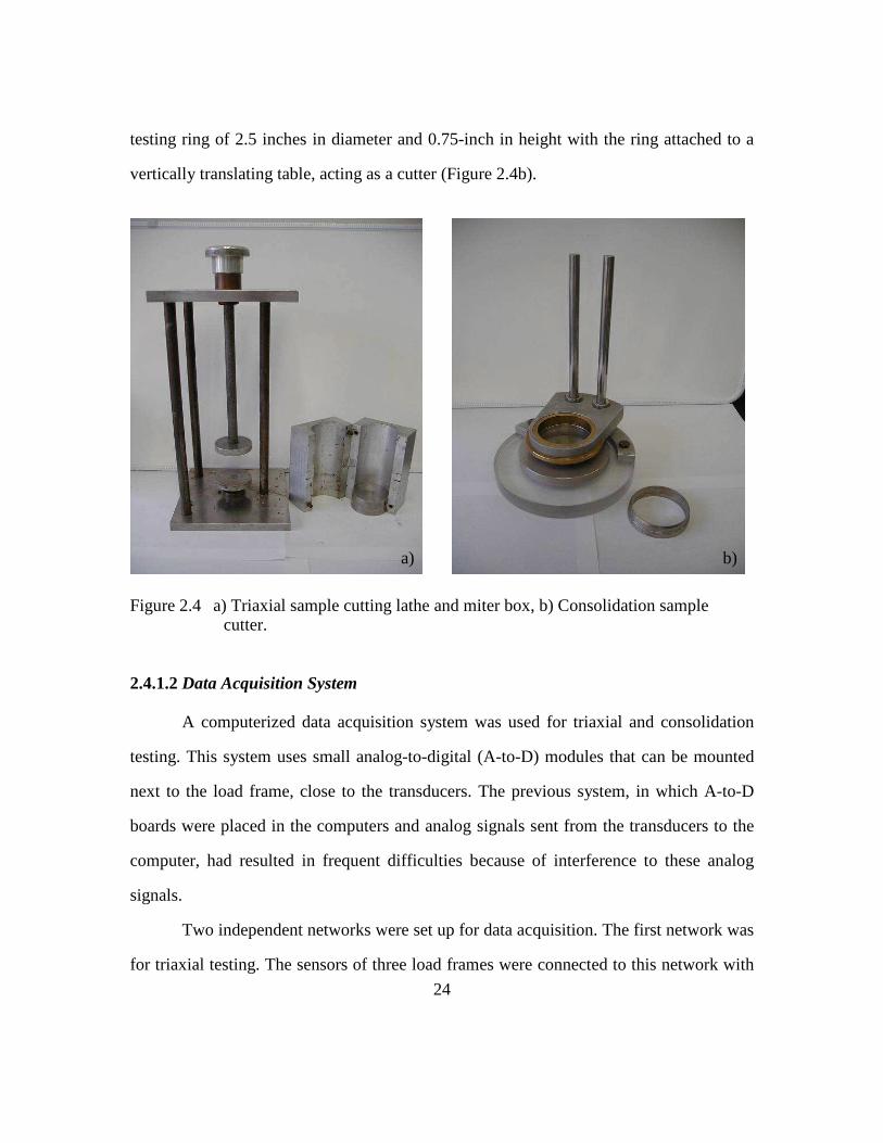
24

testing ring of 2.5 inches in diameter and 0.75-inch in height with the ring attached to a

vertically translating table, acting as a cutter (Figure 2.4b).

Figure 2.4 a) Triaxial sample cutting lathe and miter box, b) Consolidation sample cutter.

2.4.1.2 Data Acquisition System

A computerized data acquisition system was used for triaxial and consolidation

testing. This system uses small analog-to-digital (A-to-D) modules that can be mounted

next to the load frame, close to the transducers. The previous system, in which A-to-D

boards were placed in the computers and analog signals sent from the transducers to the

computer, had resulted in frequent difficulties because of interference to these analog

signals.

Two independent networks were set up for data acquisition. The first network was

for triaxial testing. The sensors of three load frames were connected to this network with

a) b)

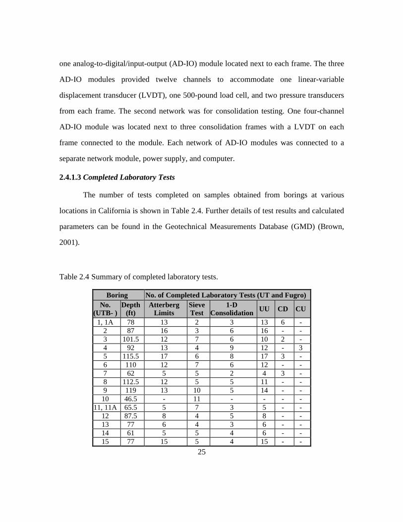
25

one analog-to-digital/input-output (AD-IO) module located next to each frame. The three

AD-IO modules provided twelve channels to accommodate one linear-variable

displacement transducer (LVDT), one 500-pound load cell, and two pressure transducers

from each frame. The second network was for consolidation testing. One four-channel

AD-IO module was located next to three consolidation frames with a LVDT on each

frame connected to the module. Each network of AD-IO modules was connected to a

separate network module, power supply, and computer.

2.4.1.3 Completed Laboratory Tests

The number of tests completed on samples obtained from borings at various

locations in California is shown in Table 2.4. Further details of test results and calculated

parameters can be found in the Geotechnical Measurements Database (GMD) (Brown,

2001).

Table 2.4 Summary of completed laboratory tests.

Boring No. of Completed Laboratory Tests (UT and Fugro) No.

(UTB- ) Depth

(ft) Atterberg

Limits Sieve Test

1-D Consolidation UU CD CU

1, 1A 78 13 2 3 13 6 - 2 87 16 3 6 16 - - 3 101.5 12 7 6 10 2 - 4 92 13 4 9 12 - 3 5 115.5 17 6 8 17 3 - 6 110 12 7 6 12 - - 7 62 5 5 2 4 3 - 8 112.5 12 5 5 11 - - 9 119 13 10 5 14 - - 10 46.5 - 11 - - - -

11, 11A 65.5 5 7 3 5 - - 12 87.5 8 4 5 8 - - 13 77 6 4 3 6 - - 14 61 5 5 4 6 - - 15 77 15 5 4 15 - -

26

Boring No. of Completed Laboratory Tests (UT and Fugro) No.

(UTB- ) Depth

(ft) Atterberg

Limits Sieve Test

1-D Consolidation UU CD CU

16 84 11 7 5 11 - - 17 89 14 3 7 13 - - 18 75.5 4 13 - 4 - - 19 70 4 9 - 6 - - 20 80 7 7 - 9 - - 21 106.5 19 1 - 19 - - 22 90.5 12 5 - 11 - - 23 102 10 5 - 18 - -

24, 24A 110 8 6 - 19 - - 25 50 - 3 - - - - 26 60 - 5 - - - - 27 45 - 5 - - - - 28 70 1 9 - 1 - - 29 50 - 5 - 1 - - 30 65 - 7 - - - - 31 65 2 2 - 2 - - 32 70 2 1 - 2 - - 33 70 - 2 - - - - 34 60 1 6 - 1 - - 35 60 1 6 - 1 - - 36 40 - 7 - - - - 37 30 - 6 - - - - 38 118.5 - 20 - - - - 39 60 2 8 - 2 - - 40 61.5 4 5 - 9 - - 41 92.5 7 7 - 22 - - 42 115 18 3 - 18 - - 43 75 12 - - 13 - - 44 141.5 12 15 - 15 - - 45 60.5 3 2 - 3 - - 46 60 2 4 - 2 - -

Total 3618.5 308 269 83 351 14 3

2.4.2 Measurements of Undrained Shear Strength, cu

2.4.2.1 Effects of Trimming on UU Triaxial Undrained Shear Strength

Unconsolidated-undrained triaxial compression tests can be performed on

untrimmed samples, i.e. as they come out of the tubes, or on trimmed samples.

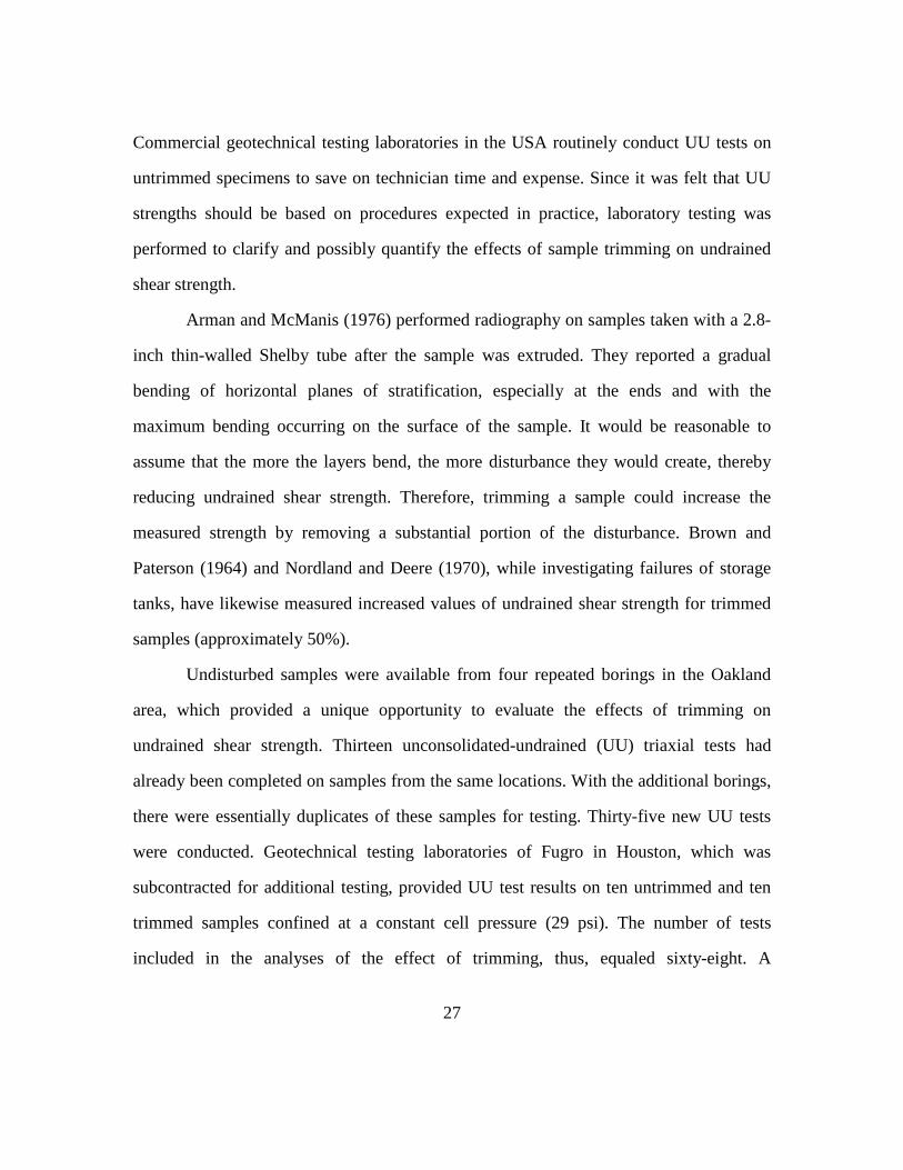
27

Commercial geotechnical testing laboratories in the USA routinely conduct UU tests on

untrimmed specimens to save on technician time and expense. Since it was felt that UU

strengths should be based on procedures expected in practice, laboratory testing was

performed to clarify and possibly quantify the effects of sample trimming on undrained

shear strength.

Arman and McManis (1976) performed radiography on samples taken with a 2.8-

inch thin-walled Shelby tube after the sample was extruded. They reported a gradual

bending of horizontal planes of stratification, especially at the ends and with the

maximum bending occurring on the surface of the sample. It would be reasonable to

assume that the more the layers bend, the more disturbance they would create, thereby

reducing undrained shear strength. Therefore, trimming a sample could increase the

measured strength by removing a substantial portion of the disturbance. Brown and

Paterson (1964) and Nordland and Deere (1970), while investigating failures of storage

tanks, have likewise measured increased values of undrained shear strength for trimmed

samples (approximately 50%).

Undisturbed samples were available from four repeated borings in the Oakland

area, which provided a unique opportunity to evaluate the effects of trimming on

undrained shear strength. Thirteen unconsolidated-undrained (UU) triaxial tests had

already been completed on samples from the same locations. With the additional borings,

there were essentially duplicates of these samples for testing. Thirty-five new UU tests

were conducted. Geotechnical testing laboratories of Fugro in Houston, which was

subcontracted for additional testing, provided UU test results on ten untrimmed and ten

trimmed samples confined at a constant cell pressure (29 psi). The number of tests

included in the analyses of the effect of trimming, thus, equaled sixty-eight. A

28

comparison of laboratory test results to determine the effects of trimming on undrained

shear strength are shown in Figure 2.5 and are summarized in Table 2.5. Undrained

strengths of trimmed and untrimmed specimens agree well at strengths less than 1000 psf

with more scatter for samples of higher UU strengths.

Undrained shear strength of trimmed specimens divided by the UU strength of

untrimmed specimens for all of the samples was 1.03 with a standard deviation of 0.29.

The average of the same ratio for samples that had been subjected to a constant cell

pressure was 0.97, with a standard deviation of 0.40. The average values compare well

with the UU tests performed at the University of Texas, which have an average ratio of

1.04. However, the standard deviation is higher than those obtained from UT testing,

which was 0.26. The effect of trimming may be better seen using the “relative error”:

( ) ( )

,

u trimmed u untrimmed

u trimmed

c c

c

−.............................................................................(2.1)

This ratio is plotted against cu(trimmed) in Figure 2.6 for all of the tests conducted. The

ratios seem to vary more or less equally about the x-axis with no obvious effect of

trimming.

Water contents and densities may vary substantially within short distances in a

soil deposit, which could have an effect on the shear strength. Although the water

contents of trimmed samples, in general, were higher than those for the untrimmed

specimens (Figure 2.7), there seems to be no obvious effect on the measured undrained

shear strength (Figure 2.8).

Part of the problem is the relatively small number of tests conducted using

untrimmed samples. In addition, the second series of borings were done because of

suspect sample quality in the first set; presumably early (trimmed specimens) tests may

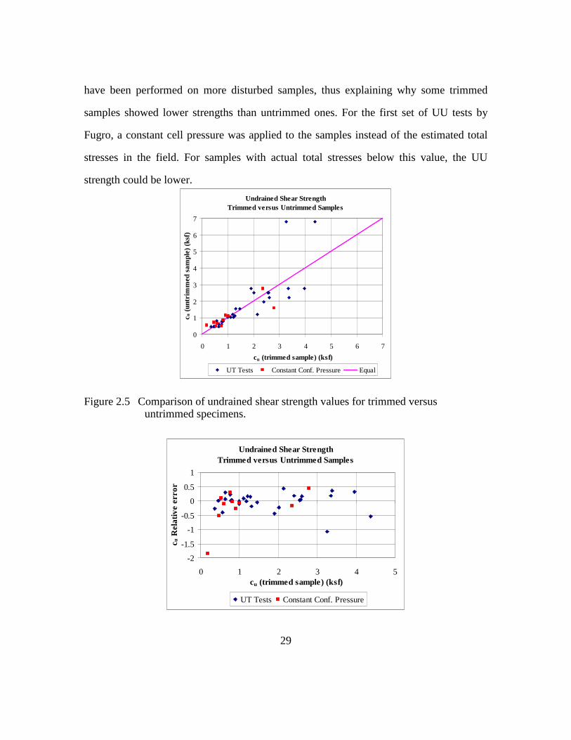
29

have been performed on more disturbed samples, thus explaining why some trimmed

samples showed lower strengths than untrimmed ones. For the first set of UU tests by

Fugro, a constant cell pressure was applied to the samples instead of the estimated total

stresses in the field. For samples with actual total stresses below this value, the UU

strength could be lower.

Undrained Shear StrengthTrimmed versus Untrimmed Samples

0

1

2

3

4

5

6

7

0 1 2 3 4 5 6 7

cu (trimmed sample) (ksf)

c u (

untr

imm

ed

sam

ple

) (k

sf)

UT Tests Constant Conf. Pressure Equal

Figure 2.5 Comparison of undrained shear strength values for trimmed versus untrimmed specimens.

Undrained Shear StrengthTrimmed versus Untrimmed Samples

-2

-1.5

-1

-0.5

0

0.5

1

0 1 2 3 4 5cu (trimmed sample) (ksf)

c u R

ela

tive

err

or

UT Tests Constant Conf. Pressure

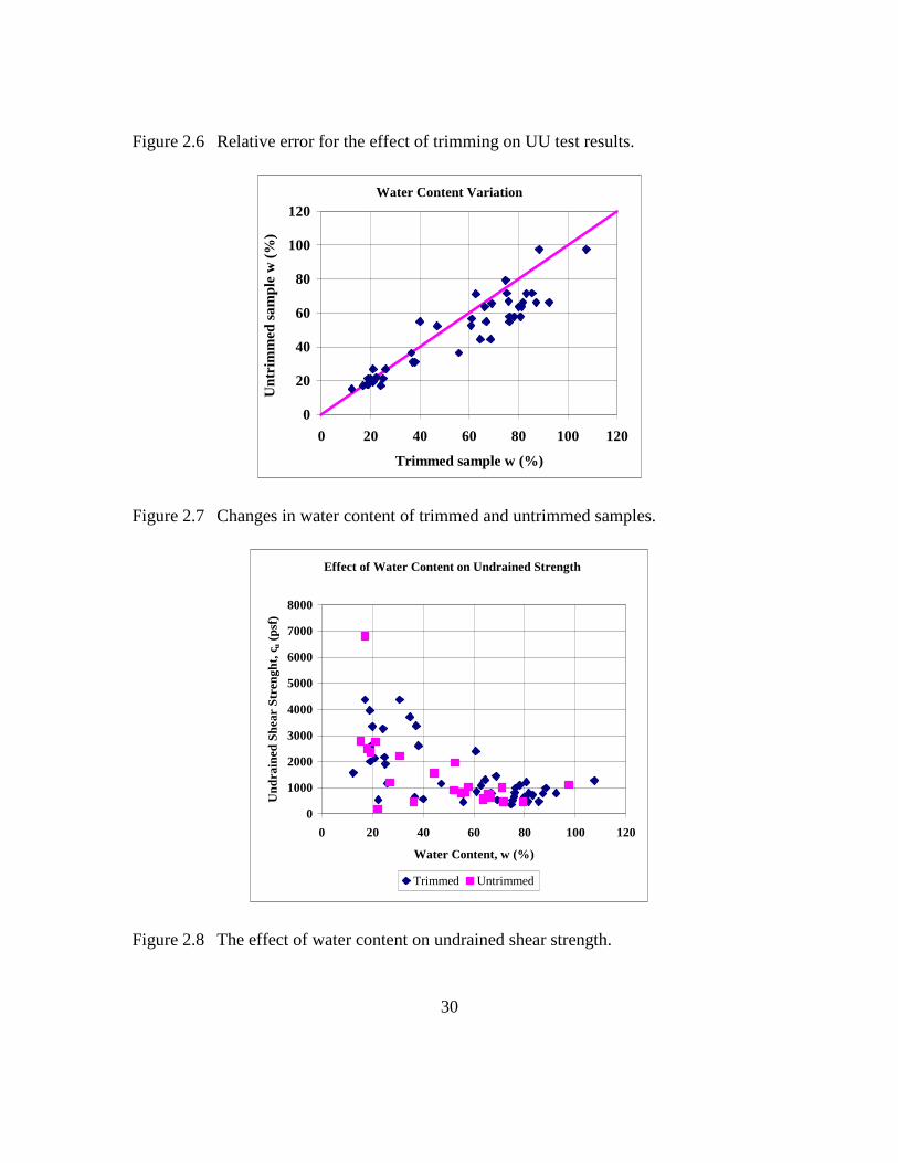
30

Figure 2.6 Relative error for the effect of trimming on UU test results.

Water Content Variation

0

20

40

60

80

100

120

0 20 40 60 80 100 120

Trimmed sample w (%)

Unt

rimm

ed s

ampl

e w

(%

)

Figure 2.7 Changes in water content of trimmed and untrimmed samples.

Effect of Water Content on Undrained Strength

0

1000

2000

3000

4000

5000

6000

7000

8000

0 20 40 60 80 100 120

Water Content, w (%)

Und

rain

ed S

hear

Str

engh

t, c u

(psf

)

Trimmed Untrimmed

Figure 2.8 The effect of water content on undrained shear strength.

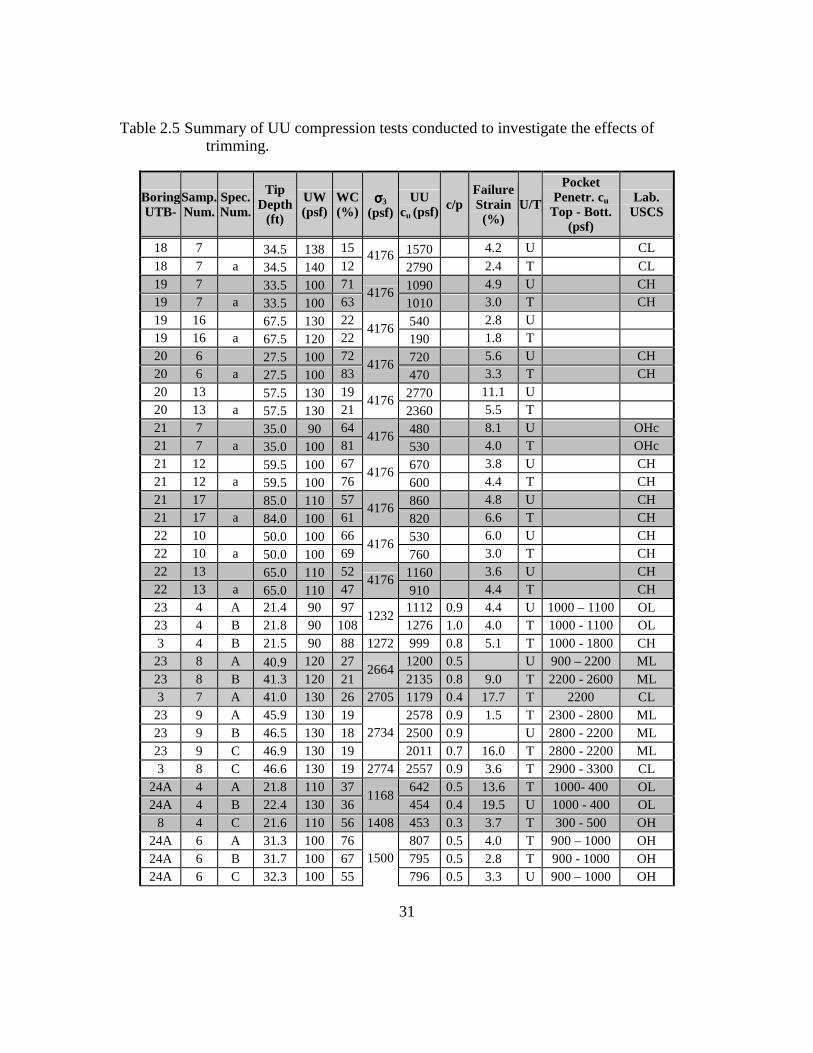
31

Table 2.5 Summary of UU compression tests conducted to investigate the effects of trimming.

BoringUTB-

Samp. Num.

Spec. Num.

Tip Depth

(ft)

UW (psf)

WC (%)

σσσσ3 (psf)

UU cu (psf) c/p

Failure Strain (%)

U/T

Pocket Penetr. cu Top - Bott.

(psf)

Lab. USCS

18 7 34.5 138 15 1570 4.2 U CL 18 7 a 34.5 140 12

4176 2790 2.4 T CL

19 7 33.5 100 71 1090 4.9 U CH 19 7 a 33.5 100 63

4176 1010 3.0 T CH

19 16 67.5 130 22 540 2.8 U 19 16 a 67.5 120 22

4176 190 1.8 T

20 6 27.5 100 72 720 5.6 U CH 20 6 a 27.5 100 83

4176 470 3.3 T CH

20 13 57.5 130 19 2770 11.1 U 20 13 a 57.5 130 21

4176 2360 5.5 T

21 7 35.0 90 64 480 8.1 U OHc 21 7 a 35.0 100 81

4176 530 4.0 T OHc

21 12 59.5 100 67 670 3.8 U CH 21 12 a 59.5 100 76

4176 600 4.4 T CH

21 17 85.0 110 57 860 4.8 U CH 21 17 a 84.0 100 61

4176 820 6.6 T CH

22 10 50.0 100 66 530 6.0 U CH 22 10 a 50.0 100 69

4176 760 3.0 T CH

22 13 65.0 110 52 1160 3.6 U CH 22 13 a 65.0 110 47

4176 910 4.4 T CH

23 4 A 21.4 90 97 1112 0.9 4.4 U 1000 – 1100 OL 23 4 B 21.8 90 108

1232 1276 1.0 4.0 T 1000 - 1100 OL

3 4 B 21.5 90 88 1272 999 0.8 5.1 T 1000 - 1800 CH 23 8 A 40.9 120 27 1200 0.5 U 900 – 2200 ML 23 8 B 41.3 120 21

2664 2135 0.8 9.0 T 2200 - 2600 ML

3 7 A 41.0 130 26 2705 1179 0.4 17.7 T 2200 CL 23 9 A 45.9 130 19 2578 0.9 1.5 T 2300 - 2800 ML 23 9 B 46.5 130 18 2500 0.9 U 2800 - 2200 ML 23 9 C 46.9 130 19

2734

2011 0.7 16.0 T 2800 - 2200 ML 3 8 C 46.6 130 19 2774 2557 0.9 3.6 T 2900 - 3300 CL

24A 4 A 21.8 110 37 642 0.5 13.6 T 1000- 400 OL 24A 4 B 22.4 130 36

1168 454 0.4 19.5 U 1000 - 400 OL

8 4 C 21.6 110 56 1408 453 0.3 3.7 T 300 - 500 OH 24A 6 A 31.3 100 76 807 0.5 4.0 T 900 – 1000 OH 24A 6 B 31.7 100 67 795 0.5 2.8 T 900 - 1000 OH 24A 6 C 32.3 100 55

1500

796 0.5 3.3 U 900 – 1000 OH

32

BoringUTB-

Samp. Num.

Spec. Num.

Tip Depth

(ft)

UW (psf)

WC (%)

σσσσ3 (psf)

UU cu (psf) c/p

Failure Strain (%)

U/T

Pocket Penetr. cu Top - Bott.

(psf)

Lab. USCS

8 6 C 31.6 110 40 1740 566 0.3 15.3 T 1100 - 1000 CL 24A 9 A 45.9 90 78 1107 0.5 4.0 T 1200 – 1100 OH 24A 9 B 46.4 90 58 1028 0.5 3.7 U 1200 - 1100 OH 24A 9 C 46.8 90 81

2076

1214 0.6 3.2 T 1200 - 1100 CH 8 9 B 46.2 100 76 2304 1000 0.4 3.8 T 1000 - 1000 CH

40 9 Head2 38.1 110 17 4379 1.9 17.5 T 3000 - 5400 ML

40 9 A 38.7 120 17 2357

6800 2.9 15.0 U 5400 – 1900 ML 11A 10 A 36.9 120 24 2264 3261 1.4 18.2 T 3600 – 3800 CL 40 13 A 51.0 140 20 3352 1.1 17.2 T 4300 – 5200 ML 41 13 B 51.4 140 19 3966 1.3 15.2 T 4300 – 5200 ML 40 13 C 52.0 120 21 2760 0.9 6.6 U 3700 – 2100 ML

11A 13 B 51.3 130 25

3109

1903 0.6 13.3 T 3000 – 5600 CL 41 5 A 22.9 130 75 356 0.3 10.5 T 600 – 600 OH 41 5 B 23.4 130 79 455 0.4 4.6 U 500 – 600 OH 41 5 C 23.9 120 86 465 0.4 3.2 T 600 – 600 OH 41 5 D 24.4 99 72

1245

467 0.4 4.2 U 500 – 500 CH 12 5 B 23.2 90 75 1294 520 0.4 3.5 T 600 – 500 CH 41 6 A 28.4 100 66 761 0.5 3.2 T 1300 – 600 OH 41 6 C 29.4 100 64

1439 601 0.4 4.6 U 700 – 700 OH

12 7 C 29.1 100 80 1457 639 0.4 3.1 T 500 – 700 OH 41 7 A 33.4 90 92 792 0.5 ? T 90 – 900 OH 41 7 B 33.9 90 66 776 0.5 3.3 U 900 – 1000 OH

41 7 C 34.3 90 82 1541

792 0.5 2.8 T 900 – 900 OH

12 8 A 32.9 90 87 1590 782 0.5 4.4 T 800 – 900 OH 41 12 A 56.2 110 31 2220 0.8 18.2 U 2600 - 2900 CL 41 12 B 56.6 110 38

2693 2613 1.0 1.6 T 3400 - 2100 CL

12 17 C 57.8 110 37 2630 3385 1.3 3.6 T 3500 – 3900 CH 41 18 A 80.6 100 61 2402 0.6 1.6 T 1900 - 1900 CH 41 18 B 81.1 100 53 1969 0.5 1.7 U 1900 - 1700 CH 41 18 C 81.6 100 64 1308 0.3 0.9 T 1900 - 1900 CH 41 18 D 82.1 100 44

4014

1552 0.4 3.3 U 1800 - 1800 CH

12 23 B 81.2 100 69 4045 1453 0.4 1.1 T 2700 - 1700 CH

UW: unit weight; WC: water content; U: untrimmed sample, T: trimmed sample. c/p: cu/σv

′, where σv′ is the effective stress.

33

2.5 SUMMARY

In this chapter, an overview of the Caltrans project, upon which this dissertation

was based, is provided. A database established within this project (FinalCT) is introduced

and evaluated in terms of its limitations and strengths. Various aspects of the site

investigation efforts are presented which were conducted to enhance/supplement the

information included in the database. Laboratory testing equipment and its calibration is

explained. Laboratory tests conducted within the project are tabulated. Special emphasis

is given to unconsolidated-undrained (UU) triaxial tests because they were used in

estimating pile capacities. Differences between the UU strength between trimmed and

untrimmed samples are shown.

34

Chapter 3: Elastic Method – Concept and Measurement of Parameters

3.1 INTRODUCTION

The “Elastic Method” is a frequently used approach, based on the theory of

elasticity for predicting the load-displacement behavior of a single pile. Mindlin’s closed-

form solution (1936) is used to calculate elastic displacements due to a vertical load

within a semi-infinite soil mass. The method is generally applied with the help of a

computer program.

In the elastic method, the utilized soil properties are Young’s modulus, Es, and

Poisson’s ratio, νs. It is usually acceptable to assume any value within the range of

possible Poisson’s ratios found in the literature (Poulos, 1989; Tatsuoka et al., 1994).

However, the effect and variability of Young’s modulus on the displacement of piles is

much more pronounced than Poisson’s ratio. Therefore, research efforts have primarily

focused on obtaining Young’s modulus through laboratory and/or in-situ measurements,

which can also be utilized to correlate with simple or commonly encountered parameters,

such as undrained shear strength, cu, and standard penetration test blow count, N. for

cohesive and cohesionless soils, respectively.

In the following sections, multiple aspects of applying the elastic method to

estimations of pile displacements will be presented and discussed.

3.2 FORMULATION OF ELASTIC METHOD

Conceptually, pile head displacement, s, can be divided into three components,

each calculated separately (Vesic, 1977):

a) Displacement of soil due to the load transmitted along the side of the pile, ρs,

b) Displacement due to axial deformation of the pile shaft, ρp, and

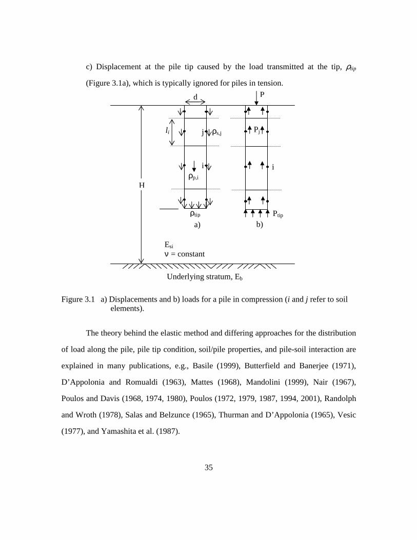
35

c) Displacement at the pile tip caused by the load transmitted at the tip, ρtip

(Figure 3.1a), which is typically ignored for piles in tension.

Figure 3.1 a) Displacements and b) loads for a pile in compression (i and j refer to soil elements).

The theory behind the elastic method and differing approaches for the distribution

of load along the pile, pile tip condition, soil/pile properties, and pile-soil interaction are

explained in many publications, e.g., Basile (1999), Butterfield and Banerjee (1971),

D’Appolonia and Romualdi (1963), Mattes (1968), Mandolini (1999), Nair (1967),

Poulos and Davis (1968, 1974, 1980), Poulos (1972, 1979, 1987, 1994, 2001), Randolph

and Wroth (1978), Salas and Belzunce (1965), Thurman and D’Appolonia (1965), Vesic

(1977), and Yamashita et al. (1987).

Esi ν = constant

Underlying stratum, Eb

d

ρs,j

l i

P

Pj

Ptip

H

i

j

i

a) b) ρtip

ρp,i

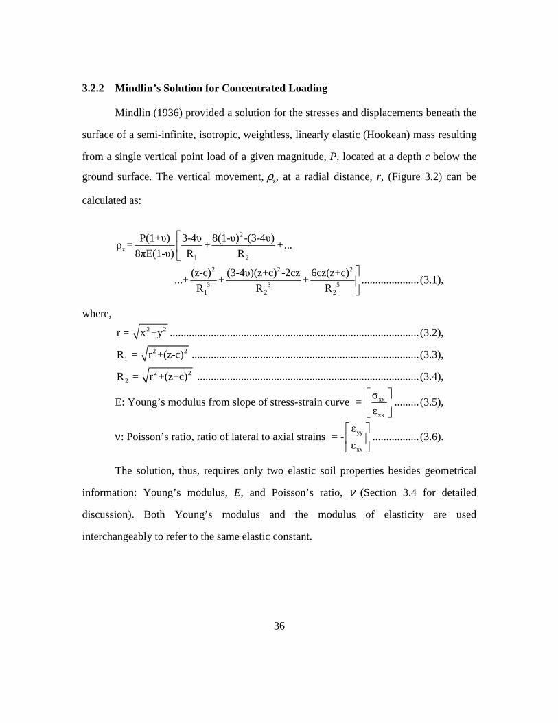
36

3.2.2 Mindlin’s Solution for Concentrated Loading

Mindlin (1936) provided a solution for the stresses and displacements beneath the

surface of a semi-infinite, isotropic, weightless, linearly elastic (Hookean) mass resulting

from a single vertical point load of a given magnitude, P, located at a depth c below the

ground surface. The vertical movement, ρz, at a radial distance, r, (Figure 3.2) can be

calculated as:

2

z1 2

P(1+υ) 3-4υ 8(1-υ) -(3-4υ)ρ = + +...

8πE(1-υ) R R

2 2 2

3 3 51 2 2

(z-c) (3-4υ)(z+c) -2cz 6cz(z+c) ...+ + +

R R R

.....................(3.1),

where, 2 2r = x +y ...........................................................................................(3.2),

2 21R = r +(z-c) ...................................................................................(3.3),

2 22R = r +(z+c) .................................................................................(3.4),

E: Young’s modulus from slope of stress-strain curve xx

xx

σ= ε

.........(3.5),

ν: Poisson’s ratio, ratio of lateral to axial strains yy

xx

ε= -

ε

.................(3.6).

The solution, thus, requires only two elastic soil properties besides geometrical

information: Young’s modulus, E, and Poisson’s ratio, ν (Section 3.4 for detailed

discussion). Both Young’s modulus and the modulus of elasticity are used

interchangeably to refer to the same elastic constant.

37

Figure 3.2 Geometry and assumptions for Mindlin’s equations (Mindlin, 1936; Poulos and Davis, 1974).

The stresses and displacements acting on the pile-soil interfaces in response to a

surface load applied to the pile are shown schematically in Figure 3.1. In reality such a

separation is an over-simplification of the pile-soil interaction problem; however, it is

helpful in establishing a framework for analysis and better understanding the factors

involved in the load-displacement behavior of piles.

Constant values can be utilized for the Young’s modulus and Poisson’s ratio of an

isotropic and homogeneous soil. Then a “displacement influence factor, Iz” (Poulos and

Davis, 1980) may be introduced for conveniently simplifying Equation (3.1) to:

z zρ =PI ...................................................................................................(3.7).

The equations for the elements that combine the pile head displacement,

displacement due to the load transmitted along the side of the pile, ρs, axial deformation

of the pile shaft, ρp, and pile tip displacement, ρtip, are given below using Eq. (3.7).

z

c

c

P

R1

r

R2

Surface

Soil: Homogeneous Isotropic Weightless Linearly elastic

x

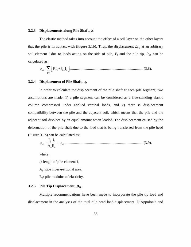
38

3.2.3 Displacements along Pile Shaft, ρρρρs

The elastic method takes into account the effect of a soil layer on the other layers

that the pile is in contact with (Figure 3.1b). Thus, the displacement ρs,ij at an arbitrary

soil element i due to loads acting on the side of pile, Pj and the pile tip, Ptip can be

calculated as: n

s,i j ij tip itj=1

ρ = P I +P I ∑ ..............................................................................(3.8).

3.2.4 Displacement of Pile Shaft, ρρρρp

In order to calculate the displacement of the pile shaft at each pile segment, two

assumptions are made: 1) a pile segment can be considered as a free-standing elastic

column compressed under applied vertical loads, and 2) there is displacement

compatibility between the pile and the adjacent soil, which means that the pile and the

adjacent soil displace by an equal amount when loaded. The displacement caused by the

deformation of the pile shaft due to the load that is being transferred from the pile head

(Figure 3.1b) can be calculated as:

jp,i s,i

p p

Pρ = ρ

A Eil = ....................................................................................(3.9),

where,

l i: length of pile element i,

Ap: pile cross-sectional area,

Ep: pile modulus of elasticity.

3.2.5 Pile Tip Displacement, ρρρρtip

Multiple recommendations have been made to incorporate the pile tip load and

displacement in the analyses of the total pile head load-displacement. D’Appolonia and

39

Romualdi (1963) and Poulos and Mattes (1969) analyzed piles allowing for no tip

displacement or load, i.e., the pile resting on a rigid base.

Poulos and Davis (1968), as well as Poulos and Mattes (1969), assumed pile tips

to be in elastic soils. The displacement at the pile tip is due to the cumulative effects of

the entire load transferred from other pile shaft elements, Pj and the load distributed along

the cross-sectional area at the pile tip, Ptip: n

tip j tj tip ttj=1

ρ = P I +P I∑ ...............................................................................(3.10).

3.2.6 Pile Head Displacement

There are (2n+2) unknowns for calculating the pile head displacement based on

the elasticity:

- (n) values of pile shaft displacements, n

s,ii=1

ρ∑

- (n) values of loads displacing the pile shaft, n

ii=1

P∑

- pile tip load, Ptip and pile tip displacement, ρtip.

Equations (3.8) through (3.10) provide (2n+1) equations. The additional

equation is for the total load within the pile: n

i tipi=1

P= P +P∑ ........................................................................................(3.11).

With the equations above, displacement can be calculated for a given load applied

to the top of the pile. Moreover, a theoretical distribution of loads along the pile length

and tip, and displacement occurring at each pile element can be investigated.

3.3 MODIFICATIONS TO ELASTIC METHOD

There are many simplifying aspects and assumptions in Mindlin’s original

solution: the vertically applied pile loads are assumed to be acting as point loads (1)

40

within a soil that is homogeneous (2), isotropic (3), initially stress-free (4), linearly elastic

(5) and a infinite half-space (6). Additionally, no slip between the pile and adjacent soil is

allowed when the solution is applied to piles (7).

Methods and recommendations to modify the elastic method for distribution of

stresses on the sides of the pile, variations in soil properties (heterogeneity), finite-depth

of soil layers, pile-soil relative displacement, rigid base for “end-bearing” piles, and

residual stresses are considered below.

3.3.1 Shear Stresses on Pile

Although all suggestions for the elastic method are based on the same principles,

there are variations proposed for handling loads transmitted to pile segments (Figure 3.3):

a) A single point load acting on the axis at the center of each pile element affects

other points along the pile (D’Appolonia and Romualdi, 1963; Salace and

Belzunce, 1965; Thurman and D’Appolonia, 1965; Basile, 1999),

b) In the disk approximation, point loads are distributed along the periphery at the

middle of the pile element (Nair, 1967), and

c) Uniform stresses are distributed along the surface of the pile element (Poulos

and Davis, 1968; Mattes and Poulos, 1969; Poulos and Mattes, 1969).

41

Figure 3.3 Shear stress distribution along the side of pile segments.

Aschenbrener and Olson (1984) have investigated the first two distributions of

shear stresses along the pile and found them to be too crude to be useful, a finding also

supported by Poulos and Davis (1980). In this dissertation, stresses are, therefore,

assumed to be uniformly distributed along the pile shaft (Figure 3.3c).

3.3.2 Non-Homogeneous Soil

Soils in nature are rarely, if ever, homogeneous. Approximations are suggested by

Poulos (1979), Lee et al. (1986), Yamashita et al. (1987), Lee and Small (1991),

Vallabhan and Mustafa (1996), and Lee and Xiao (1999) to improve the solutions

obtained through the elastic method and bring the theoretical approach closer to cases

encountered in practice. Overall, they all involve some form of a modification to Young’s

modulus incorporated into Eq. (3.1).

The effects of a pile element on other pile elements are taken into consideration in

the elastic method. When a pile element is deforming, other pile elements are also

affected to some degree by the same loading. This interaction can be represented in the

a) Point load

b) Circular line load

c) Uniformly distributed

h

h/2

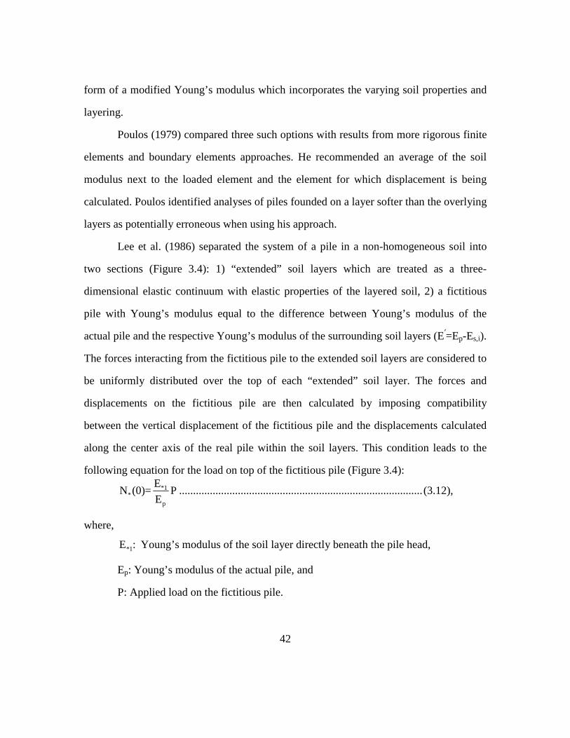
42

form of a modified Young’s modulus which incorporates the varying soil properties and

layering.

Poulos (1979) compared three such options with results from more rigorous finite

elements and boundary elements approaches. He recommended an average of the soil

modulus next to the loaded element and the element for which displacement is being

calculated. Poulos identified analyses of piles founded on a layer softer than the overlying

layers as potentially erroneous when using his approach.

Lee et al. (1986) separated the system of a pile in a non-homogeneous soil into

two sections (Figure 3.4): 1) “extended” soil layers which are treated as a three-

dimensional elastic continuum with elastic properties of the layered soil, 2) a fictitious

pile with Young’s modulus equal to the difference between Young’s modulus of the

actual pile and the respective Young’s modulus of the surrounding soil layers (E′=Ep-Es,i).

The forces interacting from the fictitious pile to the extended soil layers are considered to

be uniformly distributed over the top of each “extended” soil layer. The forces and

displacements on the fictitious pile are then calculated by imposing compatibility

between the vertical displacement of the fictitious pile and the displacements calculated

along the center axis of the real pile within the soil layers. This condition leads to the

following equation for the load on top of the fictitious pile (Figure 3.4):

*1*

p

EN (0)= P

E.......................................................................................(3.12),

where,

*1E : Young’s modulus of the soil layer directly beneath the pile head,

Ep: Young’s modulus of the actual pile, and

P: Applied load on the fictitious pile.

43

Lee et al. (1986) provided a solution with design charts for a system which

requires transforming a multilayered soil into a two-layer system depending on the

contribution from each layer based on its thickness. This approach appears rather

cumbersome and impractical since most piles are driven in soil layers with multiple

thicknesses and properties.

Figure 3.4 Problem definition by Lee et al. (1987) a) Axially loaded pile in a layered soil, b) Extended soil layers, c) fictitious pile.

Yamashita et al. (1987) argued that ignoring the soil elastic modulus of strata

other than those two interacting, as Poulos (1979) had suggested, gives results that are in

error when the soil modulus of layers differ significantly from each other. Therefore, they

proposed including weighted averages of Young’s modulus for other layers based on

layer thickness, when calculating the equivalent Young’s modulus. Their analyses result

in displacement estimations about 10% closer to those obtained from finite element

analyses than what would be found by using Poulos’ recommendation.

44

A method based on finite-layer analysis was proposed by Lee and Small (1991) as

a simplified alternative to other more elaborate elastic continuum methods. They

considered the soil as a series of horizontal, isotropic or cross-anisotropic elastic layers of

infinite lateral extent, imposing compatibility between the displacement of the pile and

soil. They assumed circular concentrated circumferential stresses acting at the middle of

each pile element similar to Nair (1967). The suggested method, compared to other

elastic continuum methods, provides similar results with less computing time.

Vallabhan and Mustafa (1996) developed a closed-form solution based on

minimizing a potential energy function using a variational approach. In this model both

soil and pile are assumed to be linearly displaced by an equal amount (compatibility).

The model distributes the work done by the applied load as compressive strain energy in

the pile and as shear energy in the soil, as well as compressive strain energy in the soil

surrounding the pile and at the bottom of the pile. The pile is assumed to be compressible

and the magnitude of the load transferred to the soil on the pile interface is calculated

based on the movement of the pile relative to the surrounding soil. Closed-form solutions

are provided by Vallabhan and Mustafa for a two-layer soil, which consists of a uniform

soil with a hard bearing stratum, a method which ignores radial displacement.

Lee and Xiao (1999) extended the method of Vallabhan and Mustafa to include

multiple sub-layers along the pile based on the actual soil profile and to incorporate the

displacement of soil mass horizontally, which can be important for designing pile groups.

3.3.3 Finite Depth of Soil Layers

Mindlin’s solution requires the soil to extend to a semi-infinite depth. In contrast,

piles sometimes have a tip on a stiff or “rigid” bearing strata. An estimate of the effects of

a finite layer on the shear and displacement of a pile is obtained by using Steinbrenner’s

45

(1934) approximation. In this approach, the displacement of a pile in a soil with a given

depth H is calculated by subtracting the pile displacement below this height from the

displacement of the same pile in a semi-infinite layer.

Poulos and Davis (1968) suggested a modification to account for stiff, but not

rigid, soil layers. In general, the displacement influence factor I ij(H) for a point within a

finite layer of depth, H can be approximated as:

ij(H) ij( ) Hj( )I I -I∞ ∞≅ ..................................................................................(3.13),

where,

Iij(∞): displacement influence factor for a pile element, i in a semi-infinite soil

mass,

IHj(∞): displacement influence factor for a point within the semi-infinite soil mass

directly beneath i, at a depth H below the surface.

The above approach can also be used to calculate displacement for a pile on a stiff

base. However, it is still an approximation. A more reliable approach for piles resting on

rigid bases is to use a “mirror-image” pile, as discussed below.

3.3.4 Piles Founded on a Rigid Base

The displacement of a pile founded on a rigid base is less than that on an elastic

base. D’Appolonia and Romualdi (1963) suggested using a “mirror-image”

approximation for piles founded on rock. The same method can be applied to other stiff

or rigid soils beneath a pile. A mirror-image pile is assumed below the actual pile at the

soil-end bearing stratum interface in which the forces equal those in the real pile but in

the opposite direction (Figure 3.5). Mindlin’s formulation is then used with additional,

opposite mirror-image forces; thus, the displacement of the actual pile is effectively

reduced to reflect the rigid base.

46

This approach produces the erroneous result that the horizontal (mirror) plane is

smooth because vertical radial displacements are the same whether arriving at the plane

from above or below, and thus there are no shearing stresses in the plane. However,

frictional forces would actually be causing shear stresses to develop in the rigid layer.

Mattes (1972) investigated radial displacement compatibility and found its effects to be

minor.

It can be argued that a very high value of Young’s modulus for the rigid layer at

the tip should be used. However, errors are likely to occur in the estimation of

displacements when there is a large variation in Young’s modulus. An averaging similar

to that recommended by Yamashita (1987) may be utilized to overcome this problem.

3.3.5 Pile-Soil Relative Displacement

The no-slip condition (displacement compatibility) at the soil-pile interface is an

essential part of calculating pile displacements using Mindlin’s solution. The pile side

capacity is limited by the soil-to-pile adhesion. It is, therefore, reasonable to allow for a

relative displacement (slip or local yielding) between the pile and soil. D’Appolonia and

Romualdi (1963), Salas (1965) and Poulos and Davis (1968) proposed a method to

incorporate a limiting stress, which can develop in the pile-soil interface. If the average

calculated shear stress on any pile element exceeds the adhesion, then local slip occurs

and the calculated shear stress is equal to the adhesion. The excess stress will be

transferred to other elements whose side shears are still less than the adhesion. The

capacity of the pile tip depends on the bearing capacity of the soil beneath the pile tip.

When all of the soil elements reach their limits, plunging will occur; i.e., pile capacity is

reached.

47

The effect of soil softening, i.e., the reduction of soil shear strength to lower

residual values following the peak value, which may lead to load shedding within pile

elements, is not taken into account using the elastic analyses discussed here. Methods

have been proposed which incorporate a reduction factor to the pile side capacity (Murff,

1980; Randolph, 1983, and Guo, 2001).

Figure 3.5 Mirror-image approach for a pile on a rigid base.

3.3.6 Residual Stresses

Load-displacement analyses are usually done assuming that no stresses due to

installation effects develop either in the pile or in the surrounding soil. However, the

Displacement calculation point

z

c

pj

R1

r

Surface

Soil: Homogeneous Isotropic Weightless Linearly elastic

x

H

H

c

c

c

pj′

R2

R3

R4

RIGID BOUNDARY

P

pj Actual Pile

Mirror Image

pj′

48

function of pile driving is, in fact, to continually cause the soil surrounding the pile to

fail, so the pile can advance into the ground to the desired depth. Thus, in actual field

conditions, the soil against the pile, as well as a certain horizontal distance away from the

pile, is sheared to large displacements and may conveniently be considered as remolded.

Some of the final driving energy (residual stresses) is locked up in the shaft as well as at

the tip of the pile. The effect of this energy for pile capacity is mainly on the distribution

of loads along the pile once loading is resumed. However, residual stresses influence the

observed displacements during a pile load test. For a pile in tension, the recorded

displacements will be smaller than the “actual, correct” values if residual stresses are not

considered. In turn, the observed displacements for a pile in compression will be in

excess of the “true” values. The residual stresses can be important mainly when

displacements are predicted for compressible piles, piles driven in sands, or piles that

derive a significant portion of their capacity from the tip (Fellenius, 2006; Maiorano et

al., 1996; Poulos, 1987; Vesic, 1977).

Methods have been proposed to estimate the residual loads and their effects on the

measured displacements (Alawneh and Husein Malkawi, 2000; Briaud and Tucker, 1984;

da Costa et al, 2001; Goble and Hery, 1984; Holloway et al., 1978; Hunter and Davisson,

1969). Another procedure to consider residual stresses due to installation effects with the

elastic method was discussed by Poulos (1987). He suggested estimating stresses by

loading the simulated pile to failure in compression and then unloading it. This cyclic

loading pattern mimics the advancement and installation of a pile. The stresses computed

in the simulated pile at the end of this cycle are then taken as the residual stresses and

represent the starting point for the subsequent analysis.

49

3.4 PARAMETERS OF ELASTIC METHOD

3.4.1 Drained versus Undrained Parameters

It may be important to distinguish between undrained and drained soil parameters

utilized for elastic method: Eu, νu or Ed, νd for undrained and drained conditions,

respectively.

For an elastic soil, the value of shear modulus is unaffected by the drainage

condition, because the water within the soil skeleton can not bear any shear stresses.

Therefore, the following can be written for the shear modulus:

uu

u

E E = G = G =

2(1+ν ) 2(1+ν).............................................................(3.14).

Poisson’s ratio, νu, for the undrained condition is equal to 0.5. Thus,

uE 3 =

E 2(1+ν)......................................................................................(3.15).

A constant Poisson’s ratio of 0.4 is used throughout this study. Then Eu/E is

3 2.8= 1.07, which is not very significant given the uncertainty of other factors involved

in elastic method.

Most of the pile load tests conducted by Caltrans follow the ASTM “quick load

method” (ASTM D-1143 1994 for compression and ASTM D-3689 1995 for tension)

using reaction piles to apply the load (California Foundation Manual, 1997). In this

method each loading increment is held for five minutes during loading and one minute

during unloading without any measurements or consideration of generated or dissipated

pore pressures. The soil is likely partially drained during pile load tests, although the

percentage of drainage is not known. Therefore in this dissertation, the Young’s modulus

50

and Poisson’s ratio adopted for all load tests correspond to soils that are partially drained

although the amount is unknown.

3.4.2 Poisson’s Ratio, ννννs

Poisson’s ratio is defined as the ratio of lateral strain to axial strain, i.e.

r

a

εν =

ε− . Under fully drained conditions, the value selected for Poisson’s ratio will

depend on the overconsolidation ratio (OCR) of clays or the relative density of sands.

Poisson’s ratio varies from nearly zero for collapsing clays and silts and for very loose

sands, to more than 0.5 for dilative soils like highly overconsolidated clays and silts and

very dense sands. Typical values of Poisson’s ratio are presented in Table 3.2. It can be

selected as (0.35±0.05) for clays under drained conditions, (0.30±0.10) for silica sands

and 0.5 for saturated clays under undrained conditions (Poulos, 1989).

Within the expected strain ranges for a pile that constitute the “working range”,

i.e. less than 0.5 % strain, the recommended drained value of Poisson’s ratio for all types

of soil is between 0.1 and 0.2 (Tatsuoka et al., 1994; Jamiolkowski et al., 1995; LoPresti

et al., 1995).

In this study, however, a constant Poisson’s ratio of 0.4 is used for all soil layers

regardless of the soil type. This approach does not conform to the recommendations of

other researchers, but the induced error is deemed to be minor.

3.4.3 Young’s Modulus of Pile, Ep

The elastic method requires only a single input for the Young’s modulus of the

pile (steel or concrete). Piles, as manufactured components, have less variability and

uncertainty in their properties than soils, for which there is usually no control over the

composition, deposition, and layering. Therefore, for elastic analyses, it seems reasonable

51

to assign a constant Young’s modulus for each type of pile. Constant Young’s modulus

values used for each pile type are given in Table 3.1.

There are several concrete-filled pipe piles within the Caltrans database.

Regardless of the loading direction, the equivalent Young’s modulus for a concrete-filled

composite steel pipe pile is calculated using the following equation, which assumes no

effect of confinement on Econcrete:

steel steel conctrete concreteeq

steel concrete

E ×A +E ×AE =

A +A......................................................(3.16),

where,

Esteel and Econcrete: Young’s modulus of steel and concrete,

Asteel and Aconcrete: cross-sectional area.

Table 3.1 Pile Young’s modulus values applied for analyses.

Pile material Steel Reinforced concrete

Unreinforced concrete

Cast-in-place concrete

Ep (kips/sq.inch) 29,000 4,500 3,000 3,000

3.4.4 Young’s (Elastic) Modulus, Es

Young’s modulus, E is defined as the slope of the stress-strain curve for a one-

dimensional, unconstrained loading:

E=ε

∆σ∆

.................................................................................................(3.17),

where, ∆σ: stress change in soil layer, and ∆ε : strains within a soil.

Young’s modulus is typically taken as the value appropriate to the strain

conditions that will occur; i.e., a value of E from seismic tests might be appropriate for

very small strains whereas values from plate bearing tests or laboratory tests could be

52

conducted on "undisturbed" samples for larger strains. Typical values of E and ν are

given in Table 3.2.

Table 3.2 Typical elastic constants of various soils (HB-17: AASHTO Standard Specifications for Highway Bridges, 17th ed., 2002).

Typical Range of Values

Soil Type/Condition Young’s Modulus, Es (kips/sq.inch) Poisson’s Ratio, ννννs

Clay Soft sensitive

Medium stiff to stiff Very stiff

0.4-2.1 2.1-6.9 6.9-13.9

0.4-0.5(undrained)

Loess Silt

All All

2.1-8.3 0.3-2.8

0.1-0.3 0.3-0.35

Fine Sand

Loose Medium dense

Dense

1.1-1.7 1.7-2.8 2.8-4.2

0.25

Sand Loose

Medium dense Dense

1.4-4.2 4.2-6.9 6.9-11.1

0.2-0.35

0.3-0.4

Gravel Loose

Medium dense Dense

4.2-1600 11.1-13.9 13.9-27.8

0.2-0.35

0.3-0.4

Young’s modulus can be found in three different ways, as shown schematically in

Figure 3.6 by a non-linear stress-strain curve typical for a soil. The laboratory and/or in-

situ methods to determine Young’s modulus also vary. The initial tangent modulus, in

particular, requires the ability to measure stresses accurately at very small strains. The

equation for each type of modulus is given below:

( )i 0

secanti

σ -σE =

ε...................................................................................(3.18),

( )( )tangent

i

d σE =

d ε.....................................................................................(3.19),

( )( )i

initialσ,ε 0

i

d σE = lim

d ε→...............................................................................(3.20).

53

Tangent, secant and initial moduli are the same at very small strains, where the

stress-strain curve can be considered linear.

Figure 3.6 Various definitions of elastic of elastic modulus: Ei: Initial tangent modulus; Es: Secant modulus; Et: Tangent modulus (defined at a given stress level).

It is, however, usually preferred in practice to use empirical correlations from

simple and/or easily obtained parameters to estimate Young’s modulus. In the case of

displacements of pile foundations, these correlations for simplicity are obtained through

back-calculations from pile load tests, relating their results to soil parameters such as SPT

blow count, cone penetration resistance, plasticity index, grain size, density, undrained

shear strength, etc.

If one can assume elasticity, then Young’s modulus, E, and axial strain, ε, can

directly be calculated from shear modulus, G, and shear strain, γ, with the following

equations: E

G=2(1+ν)

..........................................................................................(3.21),

γ=(1+ν)ε .............................................................................................(3.22),

Stress, σ

Strain, ε

1

1

1

Ei

Et

Es

54

where, ν, is Poisson’s ratio. Thus, according to the theory of elasticity, any variation of

shear modulus with shear strain also corresponds to changes in Young’s modulus and

axial strain. If the shear modulus is known, then Young’s modulus can also be calculated

by assuming a Poisson’s ratio.

Shear modulus can also be calculated as the initial small strain shear modulus

using shear wave velocity, vs, and soil density, ρ (or unit weight, γ and gravitational

acceleration, g), as: 2 2

s s

γG=ρv v

g= ....................................................................................(3.23).

Shear modulus has traditionally been used for analyzing the dynamic behavior of

soils at small strains, such as investigating foundation vibrations or seismic conditions.

However, estimating pile displacements usually involves larger strains at the affected

zones. The tangent shear modulus at small shear strains (up to about 10-3 %) is referred to

as the maximum shear modulus or small-strain modulus Gmax (or Go). Soils behave in a

linearly elastic manner within these strains. Maximum shear modulus is a unique

property of a soil regardless of drainage (drained or undrained), loading direction,

saturation, and static or dynamic conditions.

Similar to Young’s modulus, secant shear modulus decreases with increasing

shear strain. The relationship between shear modulus and strain is generally normalized

by the ratio of shear modulus to Gmax (Figure 3.7).

Geophysical methods are used to predict small-strain shear modulus of soils.

Their limitations are discussed further in Section 3.6.3.6. The most important aspect of

the conversion from shear modulus to Young’s modulus for displacement calculations of

pile foundations is the difference in the corresponding strains. While the shear modulus

reflects the elastic stress-strain behavior at small to very small strains (in the range of 10-3

55

%), the strain corresponding to pile foundation displacements at working loads is

approximately ten to a hundred times larger (about 0.1 %). Therefore, it is crucial that the

shear modulus be reduced by utilizing a corresponding modulus reduction curve.

Figure 3.7 A schematic for the normalized shear modulus – shear strain relationship.

3.4.5 Importance of Poisson’s Ratio versus Young’s Modulus

How varying Poisson’s ratio and Young’s modulus affects the predicted

displacements is presented in Figure 3.8 to depict the relative importance of each

parameter. A pile load test driven in soils with soft, clayey layers (0.5 ksf ≤ cu ≤ 0.9 ksf)

was selected (LTN: 447) to emphasize the changes in displacements. Poisson’s ratios

were varied from 0.05 to 0.5 while Young’s modulus was also changed tenfold for each

layer (35 to 626 psf). If the same Young’s modulus is used, the difference between the

two calculated displacements is not significant, approximately 5-7%. On the other hand,

the differences are significantly larger when Young’s modulus is varied for a given value

of Poisson’s ratio. A tenfold increase of Young’s modulus reduces the calculated

displacements by eighty-seven percent, when a constant Poisson’s ratio is utilized.

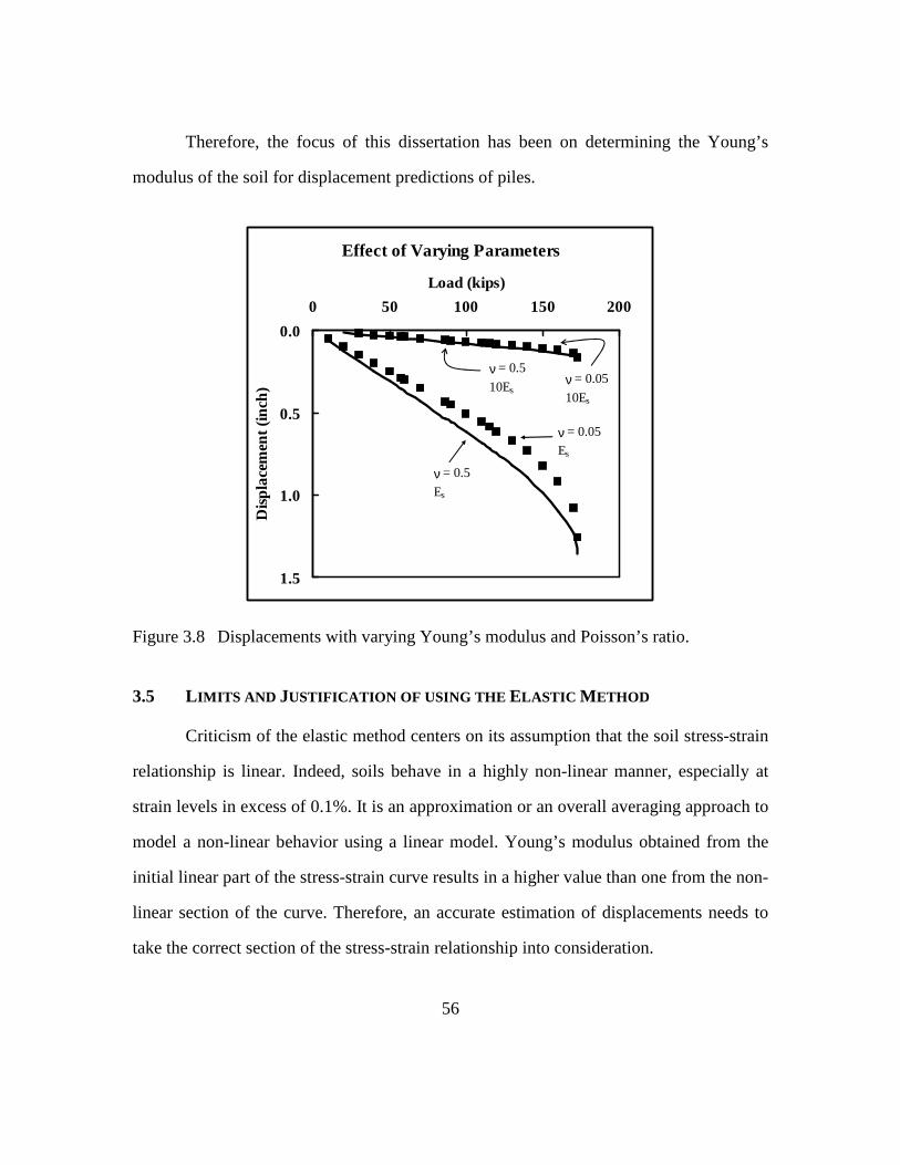
56

Therefore, the focus of this dissertation has been on determining the Young’s

modulus of the soil for displacement predictions of piles.

Effect of Varying Parameters

0.0

0.5

1.0

1.5

0 50 100 150 200

Load (kips)D

ispl

acem

ent (

inch

)

ν = 0.5

Es

ν = 0.05

Es

ν = 0.5

10Esν = 0.05

10Es

Figure 3.8 Displacements with varying Young’s modulus and Poisson’s ratio.

3.5 L IMITS AND JUSTIFICATION OF USING THE ELASTIC METHOD

Criticism of the elastic method centers on its assumption that the soil stress-strain

relationship is linear. Indeed, soils behave in a highly non-linear manner, especially at

strain levels in excess of 0.1%. It is an approximation or an overall averaging approach to

model a non-linear behavior using a linear model. Young’s modulus obtained from the

initial linear part of the stress-strain curve results in a higher value than one from the non-

linear section of the curve. Therefore, an accurate estimation of displacements needs to

take the correct section of the stress-strain relationship into consideration.

57

Another criticism is the fact that the effects of pile installation, such as soil

disturbance in an unspecified zone around the pile and sustained residual stresses

following the completion of pile driving, are not considered. In other words, the pile is

“wished-into-place” without any soil disturbance or locked-in residual stresses. Residual

stresses, in general, do not have a significant effect on the ultimate capacity. The main

concern with ignoring the residual stresses in analyses is due to the distribution of loads

along the pile shaft and the errors associated with displacements especially for

compressible piles in sand. The residual stresses are ordinarily not measured during a pile

load test. Piles are generally instrumented only at the top (head of pile) following the

installation of the test pile and data recording is started just before the application of the

load although the pile is under the influence of residual stresses.

Strain softening or load shedding is a phenomenon, in which soils exhibit a loss of

their overall shear strength towards a residual value with increasing deformation, after a

peak strength level has been reached (Murff, 1980; Sterpi, 1999). In elastic analyses,

displacements after the peak load may be underestimated, when no provision is made for

load-shedding or strain-softening behavior of soils such as overconsolidated clays, dense

sands or rocks (Randolph, 1983). The shear strength included in calculating

displacements following the peak value will be too high resulting in reduced

displacements, and, hence underestimation of actual displacements.

The analytical method involves the assumption of “no slip” between the pile and

the soil, up to the shear strength of each soil layer (elastoplastic behavior). Even after a

relative movement between pile and surrounding soil (“slippage”) occurs, the zone

affected by the pile movement can not accurately be estimated using elastic analysis

(Johnston, 1983; Poulos, 1989; 1994).

58

Similarly, Young’s modulus and Poisson’s ratio back-calculated from pile load

tests may not match values from laboratory tests because of factors such as

remolding/densification of soil next to the pile during installation, sample disturbances,

scaling, differences in the stress-strain condition, etc. (Jardine et al., 1984, 1985;

Tatsuoka and Shibuya, 1992).

In spite of all the shortcomings of the elastic method, it is still widely used due to

its relative simplicity. Modifications addressing some of the limitations are available.

Based on load tests conducted on instrumented piles (model/full-scale) supported by

numerical analyses, strains associated with most geotechnical applications and soils

within the working range are not very large: conventionally about 0.1% near the top of

the pile and less with increasing depth (Butterfield and Abdrabbo, 1983; Poulos, 2001).

Linear displacements up to about a third or half of failure load are observed from load-

displacement curves of pile load tests conducted to failure. Therefore, an “axial working

load” can be identified, under which the displacements of a pile can reasonably be

calculated with the assumption of linear elasticity. Elastic methods have been shown to

provide displacement predictions that are in satisfactory agreement with more rigorous

solutions, such as finite element or finite difference methods and do not require so many

parameters to be determined (Burland, 1989; Callanan and Kulhawy, 1985; Cooke et al.,

1979; Poulos and Davis, 1980; Poulos, 1989). This simplified approach corresponds to

the commonly available amount and sophistication of data available for most

geotechnical designs emphasized by Barbour and Krahn (2004).

An example for the linearity of load-displacement estimations within half of the

peak applied load, i.e., load ratio of a half, is presented in Figure 3.9 along with the

measured displacements. The peak load applied on the pile is varied by ±25% of the

59

measured peak load. The load-displacement curves are obtained when the load ratio is a

half. The curve for all of the utilized loads remains linear for a load up to 100 kips. This

value is 77%, 58%, and 46% of the reduced, actual, and increased peak loads,

respectively. The fit between estimations and the measured load-displacements curve is

considered excellent. Thus, even if the determined peak load is in error of 25%, the

estimated displacements are within the linear zone, which can be represented with the

elastic method.

0

0.1

0.2

0 100 200

Load (kips)

Dis

pla

cem

ent (

inch

)

75% PLPeak Load, PL125% PLMeasured

Figure 3.9 An example for the effect of varying ultimate capacity on the load-displacement curve.

60

In the following section, a general overview of laboratory and in-situ tests to

determine Young’s modulus, as well as several empirical correlations suggested in the

literature, will be presented.

3.6 DETERMINATION OF YOUNG’S MODULUS

Advantages of full-scale pile load tests can be listed as: testing under actual soil

conditions at the location of interest, the possibility of controlling and updating design

parameters and estimations of capacity and displacements, gaining experience in the area,

etc. On the other hand, the boundary conditions in a pile test are ill-defined so that they

cannot be controlled efficiently or conveniently. Pile load tests are not conducted as part

of the routine design process, especially in the preliminary stages, due to the time and

relative expense involved. Even if they are performed, piles are generally not loaded to

failure and often little information on soil properties is collected as part of the testing

process. Other means of predicting pile displacements, such as empirical correlations to

in-situ measurements and/or laboratory testing (Figure 3.10) may be preferred for small

projects or preliminary evaluations. The predicted displacements based on various

correlations, the range of strains they impose, and the ease with which they are applied

varies widely (Figure 3.11).

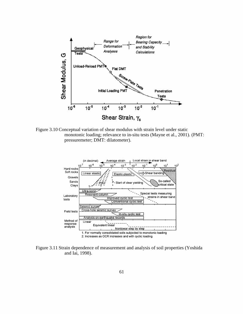
61

Figure 3.10 Conceptual variation of shear modulus with strain level under static monotonic loading; relevance to in-situ tests (Mayne et al., 2001). (PMT: pressuremeter; DMT: dilatometer).

Figure 3.11 Strain dependence of measurement and analysis of soil properties (Yoshida and Iai, 1998).

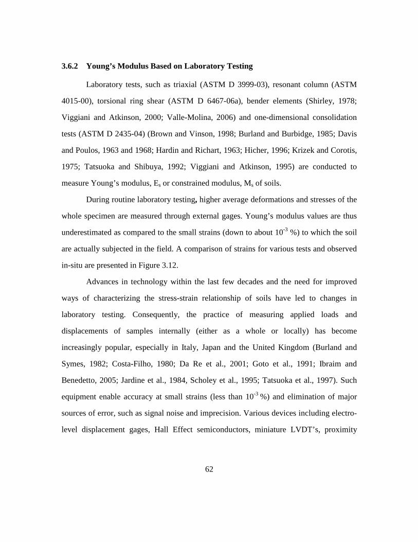
62

3.6.2 Young’s Modulus Based on Laboratory Testing

Laboratory tests, such as triaxial (ASTM D 3999-03), resonant column (ASTM

4015-00), torsional ring shear (ASTM D 6467-06a), bender elements (Shirley, 1978;

Viggiani and Atkinson, 2000; Valle-Molina, 2006) and one-dimensional consolidation

tests (ASTM D 2435-04) (Brown and Vinson, 1998; Burland and Burbidge, 1985; Davis

and Poulos, 1963 and 1968; Hardin and Richart, 1963; Hicher, 1996; Krizek and Corotis,

1975; Tatsuoka and Shibuya, 1992; Viggiani and Atkinson, 1995) are conducted to

measure Young’s modulus, Es or constrained modulus, Ms of soils.

During routine laboratory testing, higher average deformations and stresses of the

whole specimen are measured through external gages. Young’s modulus values are thus

underestimated as compared to the small strains (down to about 10-3 %) to which the soil

are actually subjected in the field. A comparison of strains for various tests and observed

in-situ are presented in Figure 3.12.

Advances in technology within the last few decades and the need for improved

ways of characterizing the stress-strain relationship of soils have led to changes in

laboratory testing. Consequently, the practice of measuring applied loads and

displacements of samples internally (either as a whole or locally) has become

increasingly popular, especially in Italy, Japan and the United Kingdom (Burland and

Symes, 1982; Costa-Filho, 1980; Da Re et al., 2001; Goto et al., 1991; Ibraim and

Benedetto, 2005; Jardine et al., 1984, Scholey et al., 1995; Tatsuoka et al., 1997). Such

equipment enable accuracy at small strains (less than 10-3 %) and elimination of major

sources of error, such as signal noise and imprecision. Various devices including electro-

level displacement gages, Hall Effect semiconductors, miniature LVDT’s, proximity

63

sensors, and local deformation transducers have been successfully utilized in triaxial

testing.

Figure 3.12 A comparison of typical strains applied in laboratory tests versus in-situ strains around structures (Clayton et al., 1995).

3.6.3 Young’s Modulus Correlations Based on In-Situ Tests

3.6.3.1 Standard Penetration Test (SPT)

The standard penetration test (SPT), which uses a split-barrel sampler, is by far

the preferred method for site investigations of cohesionless soils in situ. The test was

developed by the Gow Construction Co. in 1902. The split-barrel sampler and procedure

for the standard penetration test are described in detail in ISSMFE (1989), BS 1377:

1990, ASTM D1586 (1999) and AASHTO T-206. The test involves advancing a split

Field strains around structures

0.0001 0.001 0.01 0.1 1 10

Axial or shear strain (%)

Conventional triaxial apparatus

E o

r G

Local measurement of axial strain

Resonant column

Geophysics

64

spoon sampler into the base of a borehole by blows from a hammer with a standard

weight of 140 pounds falling from a height of 30 inches. The number of blows under

dynamic penetration for a distance of eighteen inches is recorded; however, only the

number of blows for the last twelve inches is included in the blow count number, N.

The first six inches are regarded as seating for the equipment. Disturbed samples can be

taken for observation and basic index testing in the laboratory.

Many factors affect the outcome of standard penetration tests. These can be

summarized as:

- differences in the diameter of the borehole and drilling,

- variations in the driving energy due to different equipment and testing

procedures and the resistance of the sampler to penetration,

- the in-situ horizontal effective stress with frictional materials, this

varying with the overconsolidation ratio (OCR) of the soil,

- the extent of pore pressure generation during penetration,

- the relative proportion of end resistance versus shearing forces along the

inner and outer sides of the sampler (Ladd et al., 1977).

Standard penetration testing is a simple and quick method for obtaining an

estimate of relative density, strength, and friction of cohesionless soils. It may also be

conducted in weathered rocks as a guide to the strength of such materials. However, it is

generally not recommended for cohesive soils. A large number of procedural errors

affecting SPT’s and their consequences are listed in the Canadian Foundation

Engineering Manual (1992).

Many correction factors are suggested to take into account the influences of

overburden, mineral content, water table location, pore pressure development, grading,

65

particle size, and horizontal effective stresses. Arguably the most important correction is

for the efficiency of the SPT hammer (donut, safety, or automatic), which typically is

adjusted to 60% (Skempton, 1986; Clayton, 1990).

A list of correlations relating SPT N to soil Young’s modulus is given in

Appendix B.

Standard penetration testing in soils coarser than sand poses a problem because

the driving shoe can get clogged and cause elevated N values. Therefore, larger driving

devices have been suggested to overcome this shortcoming, e.g., the Large Penetration

Test (LPT) and Becker Penetration Test (BPT). Correlations of these tests with the SPT

have been proposed by Daniel et al. (2003) and Sy (1997). The application of these

modified SPT’s is not yet widespread, however.

3.6.3.2 Cone Penetration Test (CPT)

The basic principle of cone penetration testing (CPT) is to push a cylindrical steel

instrumented conical tip and rods into the soil at a constant rate of 0.8 inch/sec (2

cm/sec). The main purpose of cone penetration test measurements is to record the

resistance to penetration mobilized in the soil. The method, developed by Collin in

France in 1846, has also been known as the static penetration test, quasi-static penetration

test, and Dutch sounding test. Current designs were mainly developed in the 1930’s. The

test is performed in accordance with ASTM D 3441 (2005) for mechanical systems and

ASTM D 5778 (2000) for electric and electronic systems. The diameter of the base of the

standard cone is 1.4 inches (35.7 mm) with a friction sleeve of 23.3 inch2 (150 cm2) and

the tip at an apex angle of 60°. The measured tip/point resistance is, qc, calculated by

dividing the total force acting on the cone tip to the area of the cone base. The side/sleeve

resistance, fs, is the total force on the friction sleeve divided by the surface area of the

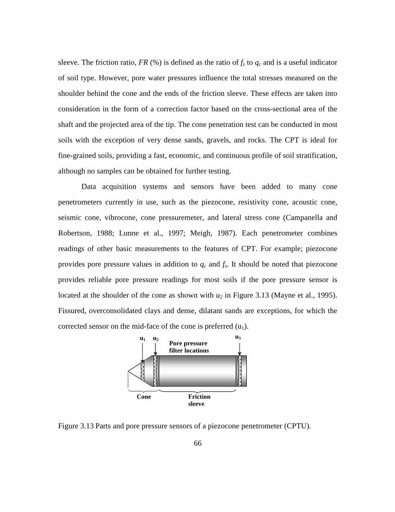
66

sleeve. The friction ratio, FR (%) is defined as the ratio of fs to qc and is a useful indicator

of soil type. However, pore water pressures influence the total stresses measured on the

shoulder behind the cone and the ends of the friction sleeve. These effects are taken into

consideration in the form of a correction factor based on the cross-sectional area of the

shaft and the projected area of the tip. The cone penetration test can be conducted in most

soils with the exception of very dense sands, gravels, and rocks. The CPT is ideal for

fine-grained soils, providing a fast, economic, and continuous profile of soil stratification,

although no samples can be obtained for further testing.

Data acquisition systems and sensors have been added to many cone

penetrometers currently in use, such as the piezocone, resistivity cone, acoustic cone,

seismic cone, vibrocone, cone pressuremeter, and lateral stress cone (Campanella and

Robertson, 1988; Lunne et al., 1997; Meigh, 1987). Each penetrometer combines

readings of other basic measurements to the features of CPT. For example; piezocone

provides pore pressure values in addition to qc and fs. It should be noted that piezocone

provides reliable pore pressure readings for most soils if the pore pressure sensor is

located at the shoulder of the cone as shown with u2 in Figure 3.13 (Mayne et al., 1995).

Fissured, overconsolidated clays and dense, dilatant sands are exceptions, for which the

corrected sensor on the mid-face of the cone is preferred (u1).

Figure 3.13 Parts and pore pressure sensors of a piezocone penetrometer (CPTU).

Cone Friction sleeve

u1 Pore pressure filter locations

u2 u3

67

Cone penetrometer testing resembles the geometrical and vertical penetration

process of the pile; therefore, its results are frequently used to estimate pile capacity. The

CPT point resistance, qc, is usually associated with the pile tip capacity, qtip, and CPT

sleeve capacity, fs, is linked with the pile side capacity, qside. CPT measurements may also

be employed in correlating Young’s modulus of the soil. Several correlations are listed in

Appendix B.

Cone penetration testing, until recently, was not part of the Caltrans “standard”

soil investigation practice and is, therefore, not available for most of the sites considered.

Some CPT conducted as part of this project could not reach the target depth due to the

presence of concrete blocks and other obstructions in shallow fills or strong clays, dense

sands, or rock at greater depths. Essentially no CPT could be completed in Southern

California where the prevalent soils are sands, gravels, and cobbles. Predrilling, i.e.,

drilling with an auger to some depth, was also attempted in many cases to pass through

the top layers; lower layers still proved too difficult to penetrate in most cases. Therefore,

CPT test results were not included in the displacement analyses of this dissertation.

3.6.3.3 Pressuremeter Test (PMT)

The pressuremeter (PMT) was first described by Ménard (1957). The PMT device

consists of two parts: a read-out unit at the ground surface and a long cylindrical probe

combining three independent cells (rubber membranes) that are inflated using a

pressurized fluid, such as water, gas or oil, after being lowered into a borehole. The top

and bottom cells protect the middle measuring cell applying pressure to the sidewalls of

the borehole. The probe can be installed by pre-drilling a hole using a hollow stem auger

or a hand auger, or forcing the probe into the ground and displacing the soil by driving,

jacking, or vibrating. Self-boring probes, generally used for research, are also available.

68

Soil disturbance occurs during the insertion of the pressuremeter device. Pressuremeter

testing and evaluation of its results are described in ASTM D 4719 (2000) and by Mair

and Wood (1987).

Once the probe is at the desired depth for testing, the top and bottom cells are

inflated to secure the probe in place. Then the measuring cell is pressurized to inflate its

flexible rubber bladder, which in turn transfers the pressure to the borehole walls. As the

pressure in the measuring cell increases, the borehole walls deform. The pressure within

the measuring cell is held constant for approximately sixty seconds, during which time

the increase of volume is recorded.

Due to the dimensions of the measuring cell (diameter between 1.25 and 3 inches,

L/D between 3 and 10, typically 6) a large soil mass can be tested vertically with the

pressuremeter to obtain parameters, which can also be a disadvantage due to the

uncertainties of averaging over a zone of disturbed soil. Entire stress-strain-strength

curves can be derived, as well as in-situ total horizontal stress, P0, shear modulus, G,

shear strength, su, or Φ, and limit pressure, pL. Types of pressuremeters include the pre-

bored (Ménard), push-in device, self-boring pressuremeter, and full-displacement type

(cone pressuremeter or pressiocone).

A pressuremeter deformation modulus, EPMT, can be calculated from the pseudo-

elastic or straight-line portion of the load-volume change diagram. The EPMT is a function

of Poisson’s ratio, the slope of the straight line and the cavity volume in the pseudo-

elastic range (part B in Figure 3.14). Martin (1977) and Gambin and Rousseau (1988)

concluded that EPMT, and soil Young’s modulus, Es, are approximately equal. Martin

(1987) has proposed three similar correlations between EPMT and SPT N.

69

Figure 3.14 Example of a pressuremeter test result (Baguelin et al., 1978).

Based on pressuremeter readings, Frank (1985) and Frank et al. (1991) have

suggested an empirical correlation which relates the pile displacements within working

loads to the pile diameter (discussed in Chapter 4).

3.6.3.4 Plate Loading Tests (PLT)

The plate loading test can be thought of as a scaled-down model of a shallow

foundation. The PLT is commonly used for cohesionless soils although it can also be

applied to cohesive soils. Furthermore, it can prove useful in assessing the properties of

weak rocks. A single or a series of steel bearing plates (to increase rigidity when large

bases are loaded) are used with a hydraulic loading jack against a truck or trailer or a

combination of both, an anchored frame, or any other structure loaded with sufficient

weight to produce the desired reaction on the surface. Extensometers are used to measure

the deflection under the load applied by jack or deadweight. The equipment and testing

procedure for PLT is described in ASTM D 1195 (1997). An equivalent soil Young’s

70

modulus, Es, can be calculated by plotting the load-displacement curve and applying the

elastic method for a uniformly loaded rigid plate on a semi-infinite elastic isotropic solid

as follows:

( )2s

s p w

p

1-υE = B I

∆ρ ∆q .............................................................................(3.24)

where,

νs : Poisson’s ratio, typically 0.4,

p

∆ρ

∆q : the slope of displacement versus plate pressure (inches/psi),

Bp : diameter of the plate, (inches) and

Iw : influence factor, π/4 for circular plates.

The estimated Young’s modulus is representative of soil within a depth of 2Bp

beneath the plate.

A reasonable objection can be raised that the shallow foundation elastic modulus

is different from that of deep foundations in that it overlooks such factors as confinement

and porewater pressure, soil layering, etc. A variation of the PLT, the screw-plate loading

test, can then be employed (Schmertmann, 1970). In a screw-plate test, an auger with an

instrumented circular plate for controlling loads and displacements is inserted into the

soil and loaded vertically. The evaluation is similar to that for PLT.

3.6.3.5 Flat Plate Dilatometer (DMT)

The flat plate dilatometer (DMT), also called Marchetti dilatometer, was first

introduced by Marchetti in 1975. It consists of a stainless steel blade with a flat,

approximately one-inch diameter circular steel membrane mounted flush on one side,

which is commonly pushed vertically into the soil. The blade is connected to a control

unit on the ground, used to record pressure changes in the diaphragm. Insertion of the

71

blade with the help of CPT or regular drill rods is followed by the inflation of the

membrane. Two readings are taken within approximately one minute of each other:

1) The “A-pressure” to push the membrane into contact with the

surrounding soil (“lift-off”)

2) The “B-pressure” to move the center of the membrane 0.04 inches (1.1

mm) against the soil.

These readings can then be repeated by pushing or driving to further depths so

that a soil profile can be obtained. Collected data need to be corrected by calibration

factors involving membrane stiffness and local geology. Correlations are utilized for

estimating design parameters, such as soil Young’s modulus or maximum shear modulus,

Gmax.

The flat plate dilatometer can be used for a wide range of soils, but not for dense

or hard materials (such as gravels) due to risk of damage to the steel membrane. ASTM D

6635 (2001) and ISSMGE Committee TC16 Report on DMT (2001) further explain the

equipment, calibration process, data collection and reduction as well as comparisons with

other in-situ tests. A geophone can be added to the dilatometer to obtain shear wave

velocity measurements alongside typical DMT parameters.

3.6.3.6 Geophysical Methods

All of the above testing methods involve the drilling of boreholes, sampling at a

few points, and laboratory or in-situ testing of soil samples. The process is typically

restricted by time and budget. The common site investigation is limited to a small portion

of the volume of soil and rock that could be sampled and tested. For this purpose,

geophysical methods, cost-effective ways of characterizing the soil, are increasingly

72

being used in conjunction with improved interpretative models. Geophysical methods can

be applied to most soils and rock.

The available geophysical methods for determining the small strain modulus of

soils can be divided into two groups (Campanella, 1994):

1) non-intrusive surface geophysics (seismic reflection/refraction/

resistivity and spectral analysis of surface waves (SASW)), and

2) conventional borehole geophysics (downhole, crosshole, crosshole

impulse, downhole nuclear and resistivity, suspension logger).

Non-intrusive geophysical surface tests have the further advantages of not

affecting the natural soil fabric during implementation and of being able to be conducted

on limited access and/or difficult test sites. The difficulty with surface tests is that no

sample is obtained as part of the method, which may lead to errors in interpreting the

results. On the other hand, borehole tests provide a sample to be evaluated but may cause

disturbance to the very surface the test is being conducted on, which could be significant

especially for measurements of small strains.

In general, the deformation modulus is determined directly or indirectly by

measuring S-waves (shear). The propagating shear wave velocities, vs, are evaluated to

determine the respective small-strain elastic shear modulus, Gmax. Water has no effect on

the measured shear wave velocities; therefore, the saturation of the tested material is not

relevant (Stokoe and Santamarina, 2000). Typical S-wave velocities of soils are between

350 fps to 2000 fps.

Shear modulus can then be converted to Young’s modulus utilizing Poisson’s

ratio and assuming elastic behavior (Section 3.4.4). However, it is necessary to apply an

appropriate reduction factor if the strains in the wave propagation do not match the

73

strains in the prototype. The shear modulus is calculated from strains that are of the order

of 10-3 %, whereas Young’s modulus appropriate for displacements of pile foundations is

within approximately 0.1 %. As shown previously, Young’s modulus values decrease

rapidly as the strains increase, thus making the adjustment critical.

A comprehensive collection of laboratory as well as in-situ correlations (mostly

for SPT blow count in sandy soils) for shear wave velocities and shear modulus have

been compiled by Sykora and Stokoe (1983).

3.6.4 Limits of Empirical Correlations

An important consideration for most methods from which empirical correlations

for soil Young’s modulus are derived is that they are almost entirely empirical and based

on a knowledge-base of local/on-site experiences and conditions over the years. It is not

unusual that the outcomes based on these correlations vary significantly from one

another, or that they are specific to only one location. Therefore, a critical approach

combined with engineering judgment, as with other real life geotechnical problems, is

very important. One might find that certain correlations do not apply to their cases or that

the usefulness of some of these equations could prove limited. Nevertheless, correlations

provide an economical and quick alternative for initial design conditions and projects

with a limited budget for site investigation, as is typical of most projects.

3.7 VARIABILITY OF PARAMETERS

In this study, empirical correlations for Young’s modulus are utilized and new

ones are suggested based on the findings from Caltrans database. The variability of

undrained shear strength, cu, and standard penetration test blow count has a direct effect

on the predicted displacements because they are correlated with Young’s modulus of the

soil.

74

3.7.1 Undrained Shear Strength Variability

Many factors affect the results of laboratory undrained shear strength, cu, testing

conducted with triaxial equipment. Aside from natural soil non-uniformity, a large

variability arises due to various disturbances that the soil sample may be subjected to

during drilling, sampling, transportation, storage and sample preparation (Kulhawy and

Mayne, 1990; Mayne et al., 2001; Ladd and DeGroot, 2003). The type of equipment used

and the experience/practices of the workers affect test results as well.

Other variability in undrained shear strength values stems from different testing

methods and their application techniques. Undrained shear strength can be measured in

the laboratory using unconfined compression tests (UC), unconsolidated undrained (UU

or Q for quick) triaxial tests, pocket penetrometer tests, and drop cone tests, or in the field

by vane tests, pressuremeter, and dilatometer. In these tests, many factors may influence

the measured cu, such as the direction of loading, boundary conditions, strain rate,

overconsolidation, degree of fissuring, etc. Many correlations exist as well to indirectly

estimate undrained shear strength from water content, Atterberg limits, SPT, CPT,

pressuremeter or dilatometer measurements, geophysical tests, etc. All these reflect the

uncertainty involved in estimating a consistent value of undrained shear strength.

Within the context of this dissertation, undrained shear strength is measured using

the unconsolidated undrained (UU or Q) triaxial compression test in accordance with

ASTM 2850 (2003).

3.7.2 Standard Penetration Test (SPT) Variability

Skempton (1986) concluded that the most important variability in SPT blow

counts is due to the energy applied to the rods. The penetration resistance is inversely

proportional to the energy transmitted down the drill rods to the split spoon sampler

75

(Schmertmann and Palacios, 1979; Skempton, 1986). Due to lack of standardization of

equipment, many types of SPT hammers are in use around the world, each transferring a

different energy to the rods. The efficiency is then defined as the ratio of the measured

energy passing through the rods over the theoretical free-fall energy (4200 pound-inch) of

a standard hammer. Commonly the standard penetration test blow counts are adjusted to

an energy efficiency of 60% as suggested by Seed et al. (1985) and Skempton (1986).

Energy losses may occur in several ways depending upon the type of hammer being

employed (Clayton, 1990).

A calibrated automatic hammer with 80% efficiency was used to conduct standard

penetration tests included in this study (Abe & Teferra, 1998; Frost, 1992). No correction

for the change in overburden pressure with depth was made.

3.8 SUMMARY

In this chapter, assumptions, modifications, and parameters required for the

elastic method are introduced along with the steps followed to estimate pile

displacements. Laboratory and in-situ methods to measure Young’s modulus are

presented. The shortcomings of approaches are highlighted.

76

Chapter 4: Database Classification and Evaluation of Displacements

4.1 INTRODUCTION

Pile load tests investigated in this study are broadly separated into three groups

based on the associated soil:

1) Piles in cohesive soils, i.e., clays and/or silts.

2) Piles in cohesionless soils: sands, gravel, cobbles and rock

3) Piles in mixed profiles, i.e., where the profiles consist of multiple layers

of various types of cohesive as well as cohesionless soils.

It should be noted here that an implicit assumption is made that each layer can be

defined by a single soil type. The main reason for this grouping is to analyze piles in a

single soil profile so as to obtain empirical multiplication factors for Young’s modulus of

the soil, Es.

All of the analyses are conducted with the help of a modified version of Tapile

computer code (Poulos, 1978; Aschenbrener and Olson, 1984).

4.2 DEFINITIONS OF SOIL TYPES

Throughout this dissertation, the term “clay” is used synonymously for “cohesive

soil” and “sand” for “cohesionless soil”.

Piles in cohesive (clayey) soils behave differently from piles in cohesionless

(sandy) soils; thus, their respective design approaches differ as well. As suggested by

Dennis and Olson (1983) for their API database, the terms cohesive and cohesionless are

used to reflect the engineering behavior and not to indicate the standard classification of

clays and sands according to the Unified Soil Classification System (USCS).

77

4.2.1 Cohesive Soils

Within the context of this dissertation, clay is defined as a soil that has the

following characteristics:

1. Clays are essentially undrained during pile driving.

2. Clays have a consolidation stage after pile driving that typically lasts for at

least a month (Caltrans data suggest that after a week the changes are not

significant, Brown (2001)).

3. In clays, relatively undisturbed samples can be obtained, which enables

laboratory strength tests on undisturbed samples to be conducted. Field tests, such

as geophysical methods, field vane, and CPT, can also be used.

4. Clays have low hydraulic conductivity; therefore, excess pore pressures can be

assumed not to have sufficient time to dissipate during quick load tests, such as

those employed for testing most of the Caltrans piles. Therefore, clayey soils are

assumed to be undrained during a load test.

4.2.2 Cohesionless Soils

Conversely, sand is defined as having the following properties:

1. Excess pore water pressures developed during driving undergo significant

dissipation during the driving process and are likely to be fully dissipated within

about 24 hours.

2. It is expensive to conduct laboratory studies on undisturbed specimens in sands,

which require special sampling techniques as well as testing and preservation

conditions. Reconstituting samples in the laboratory is also difficult, because

important properties depend on density, which is difficult to measure in-situ.

78

Consequently, it is preferable to design piles in sandy soils based on in-situ

testing, e.g., standard penetration test, cone penetration test, etc.

3. Sands can be assumed to be drained during a pile load test.

The term sand also encompasses materials classified as non-plastic silts, gravels,

and cobbles.

4.2.3 Mixed Profiles

Most of the soil deposits encountered in practice are heterogeneous in

composition. The properties and behavior of these soil layers may vary both vertically

and horizontally based on natural processes, such as deposition, weathering, aging,

cementation, chemical and mineralogical composition, etc., and on human effects, such

as pre-loading, dewatering, excavating, and various improvement techniques.

“Mixed profiles” describes heterogeneous soils with any combination and number

of cohesive and cohesionless soil layers. An important assumption is that each layer can

be depicted as either cohesive or cohesionless. Eighty-three out of 144 (58%) pile load

tests analyzed within the FinalCT database are driven into mixed soil profiles.

4.3 DEFINITIONS OF TERMS USED FOR COMPARISON

The ratio of any given pile load to the peak load is defined as the “mobilized load

ratio” or, in short, the “load ratio”. Correlations are utilized to obtain Young’s modulus

which is used to calculate pile head displacements with the elastic method (sc). The term

“displacement ratio” denotes the ratio of calculated displacement, sc to the measured

displacement, sm, obtained from the pile load test (sc/sm). The subtraction of sm from sc

(sc-sm) is referred to as the “displacement difference” in this dissertation and negative

values for displacements in tension tests are used directly, i.e., the actual values not the

absolute ones. Correlations are evaluated independently from one another in order to

79

establish a range of loading ratios for which Young’s modulus values may be used

successfully.

4.4 ANALYTICAL PROCEDURE USING MODIFIED TAPILE

In the following paragraphs, loads applied to a pile are shown with the symbol Q

and displacements are given as S (positive for downwards movement). The loads at

various percentages of applied peak load, Qmax, are symbolized as Qi, with i equal to a

third, a half and two-thirds. Displacements experienced when Qi are applied are shown as

Si.

The following steps are used in the analysis of pile load test data based on the

elastic method:

1. The displacement at a third, a half, and two-thirds of peak measured load is

obtained from pile load tests. These loading ratios (Qi/Qmax) correspond to the

inverse of safety factors, FS, i.e. [ ] [ ]i maxQ Q 1 FS= .

2. Pile weight is included in analyses.

3. The shear strength of the soil on the side of the pile as well as at the tip of the pile is

adjusted iteratively until the calculated pile capacity matches the measured capacity.

The tip capacity in tension is assumed to be zero. Pile capacity is calculated using

the α method (Dennis and Olson, 1983) for clayey soils and using Brown’s (2001)

modification of Fleming’s (1992) method for sands/gravels. Brown’s method was

derived directly from the same Caltrans database used in this dissertation.

4. Suggested correlations found in the literature are employed to predict displacements

to assess their applicability.

5. As a simplified approach to estimating displacements, Young’s modulus can be

assumed to be a linear function of the undrained shearing strength (cu) in cohesive

80

soils (clays and silts) and the standard penetration resistance (N) in cohesionless

soils (sands, gravel, cobbles).

The linear relationships are expressed as:

s 1 uE =K ×c (cohesive soils)................................................................. (4.1),

or

s 2 60E =K ×N (cohesionless soils) ..........................................................(4.2),

where,

cu : undrained shear strength of the soil,

N60 : standard penetration test blow count adjusted to an applied energy

of 60% (blows/foot, also given as bpf),

K1 and K2 : empirical multiplication factors for cohesive (dimensionless) and

cohesionless soils (ksf/bpf), respectively.

6. The subset of data for a single soil type is analyzed first for developing an

independent correlation for Young’s modulus, i.e. piles driven in only cohesive or

cohesionless soils. The displacements at a third, a half, and two-thirds of peak load

are matched using a trial-and-error approach by changing the multiplication factors

for Young’s modulus. Multiplication factors for each test are collected to obtain a

reasonable value for cohesive as well as cohesionless soils.

7. Piles driven into mixed soil profiles are analyzed with the multiplication factors

obtained from the previous step up to half of the peak applied load.

Predrilled or cased piles are considered to have no soil side shear strength along

the length of the predrilling or casing.

Tapile was written to accept piles that are cylindrical in shape. The diameter of

piles other than pipe piles were adjusted to an equivalent pipe pile diameter to calculate

81

the circumference and cross-sectional area correctly, as shown in Eq.s (4.3) through

(4.6).

sqeq

4DD

π= (square pile, for circumference).......................................(4.3),

sqeq

2DD

π= (square pile, for tip area) ..................................................(4.4),

s,Heq

12AD

π= (H-pile, for circumference)............................................(4.5),

c,Heq

AD 2

π= × (H-pile, for tip area)..................................................(4.6),

where,

Deq : equivalent circular diameter (inch),

Dsq : square pile width (inch),

As,H : steel-to-soil surface area of H-pile (ft2/ft),

Ac,H : cross-sectional area of H-pile (inch2).

The steel-to-soil contact area is used to calculate the circumference for H-piles.

The circumference is used for the calculation of side capacity whereas the solid pile tip

area is used for the tip capacity.

4.5 L IST OF PILE LOAD TESTS

In this section, tests utilized for displacement analyses using the elastic method

are listed for each soil type with further details provided in Appendix A. The analyses

include fine grained (cohesive clays/silts), coarse grained (sands, gravels, boulders, non-

cohesive silts/clays) and mixed (a combination of fine- grained and coarse-grained soils).

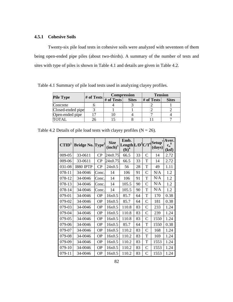
82


Twenty-six pile load tests in cohesive soils were analyzed with seventeen of them

being open-ended pipe piles (about two-thirds). A summary of the number of tests and

sites with type of piles is shown in Table 4.1 and details are given in Table 4.2.

Table 4.1 Summary of pile load tests used in analyzing clayey profiles.

Compression Tension Pile Type # of Tests # of Tests Sites # of Tests Sites

Concrete 6 4 3 2 1 Closed-ended pipe 3 1 1 2 2 Open-ended pipe 17 10 4 7 4 TOTAL 26 15 8 11 7

Table 4.2 Details of pile load tests with clayey profiles (N = 26).

CTID 1 Bridge No. Type2 Size (inch)3

Emb. Length

(ft) 4 L/D 5C/T6 Setup7

(days)

Aver. cu

8 (ksf)

009-05 33-0611 CP 24x0.75 66.5 33 C 14 2.72 009-06 33-0611 CP 24x0.75 66.5 33 T 14 2.72 031-08 I880 IPTP CP 24x0.5 56 28 T 49 1.11 078-11 34-0046 Conc. 14 106 91 C N/A 1.2 078-12 34-0046 Conc. 14 106 91 T N/A 1.2 078-13 34-0046 Conc. 14 105.5 90 C N/A 1.2 078-14 34-0046 Conc. 14 105.5 90 T N/A 1.2 079-01 34-0046 OP 16x0.5 85.7 64 T 170 0.38 079-02 34-0046 OP 16x0.5 85.7 64 C 181 0.38 079-03 34-0046 OP 16x0.5 110.8 83 C 233 1.24 079-04 34-0046 OP 16x0.5 110.8 83 C 239 1.24 079-05 34-0046 OP 16x0.5 110.8 83 C 1550 1.24 079-06 34-0046 OP 16x0.5 85.7 64 T 1550 0.38 079-07 34-0046 OP 16x0.5 110.2 83 C 168 1.24 079-08 34-0046 OP 16x0.5 110.2 83 T 169 1.24 079-09 34-0046 OP 16x0.5 110.2 83 T 1553 1.24 079-10 34-0046 OP 16x0.5 110.2 83 C 1553 1.24 079-11 34-0046 OP 16x0.5 110.2 83 C 1553 1.24

83

CTID 1 Bridge No. Type2 Size (inch)3

Emb. Length

(ft) 4 L/D 5C/T6 Setup7

(days)

Aver. cu

8 (ksf)

098-01 34-0088 OP 24x0.75 79 40 C 35 0.703 098-02 34-0088 OP 24x0.75 79 40 T 35 0.703 098-03 34-0088 OP 24x0.75 78 39 C 33 0.703 098-04 34-0088 OP 24x0.75 78 39 T 33 0.703 100-01 34-0088 OP 24x0.75 81 41 C 14 0.76 100-02 34-0088 OP 24x0.75 81 41 T 14 0.76

118L-01 28-0056 Conc. 12 64 64 C 4 1.5 122L-01 22-0062 Conc. 12 49.3 49 C 19 2.54

1 A unique number given to each test based on the order the Caltrans reports were delivered. 2 Pile type: Conc. = Concrete; CP = closed-ended pipe pile; OP = open-ended pipe pile HP = H-pile (or I-pile); Comp. = composite pile (combining two or more pile types). 3 Pile diameter for solid piles or outside diameter and wall thickness for pipe piles. 4 Embedment length, portion of pile below ground. (equal to pile length when stick-up is added). 5 Pile length to diameter ratio. 6 The direction of loading, compression or tension. 7 The time between the installation of the test pile and load testing. N/A for unknown times. 8 Average undrained shear strength along the shaft of the pile.


The list of pile load tests included in analyses for cohesionless soils is

summarized in Table 4.3 and given in Table 4.4. Open-ended pipe piles again constitute

more than half of the 34 pile load tests investigated.

Table 4.3 Summary list of pile load tests analyzed (sandy soils).

Compression Tension Pile Type # of Tests # of Tests Sites # of Tests Sites

Composite 2 2 2 --- --- Concrete 8 3 1 5 5 Closed-ended pipe 1 1 1 --- --- Open-ended pipe 19 10 6 9 4 H-pile 4 1 1 3 3 TOTAL 34 17 11 17 12

84

Table 4.4 List of pile load tests in sandy profiles (N = 34).

CTID Bridge No. Type Size (inch)

Emb. Length

(ft) L/D C/T

Aver. N60

1 (bpf)

026-01 49-0133 Conc. 14 20 17 T 40 035-01 57-0488 OP 14x0.375 26.6 23 C 31 035-02 57-0488 OP 14x0.375 26.6 23 T 31 040-05 I880 IPTP OP 24x0.75 28 14 C 83 040-11 I880 IPTP OP 24x0.75 28 14 T 73 041-01 I5/I8 IPTP OP 16x0.5 43.2 32 C 25 041-02 I5/I8 IPTP OP 16x0.5 43.2 32 T 25 041-03 I5/I8 IPTP OP 16x0.5 91.1 68 T 20 041-04 I5/I8 IPTP OP 14x0.438 85 73 T 17 041-05 I5/I8 IPTP OP 14x0.438 37 32 C 20 041-06 I5/I8 IPTP OP 14x0.438 37 32 T 20 041-07 I5/I8 IPTP OP 16x0.5 95.5 72 C 17 041-08 I5/I8 IPTP OP 16x0.5 95.5 72 T 17 041-09 I5/I8 IPTP OP 16x0.5 92.5 69 T 26 041-11 I5/I8 IPTP OP 14x0.438 89.5 77 C 15 041-12 I5/I8 IPTP OP 14x0.438 89.5 77 T 15 042-03 54-0967 HP 14x89 39 81 C 57 042-04 54-0967 HP 14x89 39 81 T 57 042-06 54-0967 HP 14x89 56 117 T 35 057-01 53-1181 HP 10x57 32 78 T 63 060-03 55-0794 Conc. 14 42.5 36 T 49 083-01 34-0046 OP 18x0.5 33 22 C 19 087-01 57-1017 Conc. 14 31 27 C 16 087-02 57-1017 Conc. 14 31 27 T 16 087-03 57-1017 Conc. 14 24 21 C 15 087-04 57-1017 Conc. 14 17 15 C 13

102L-01 51-0273 Conc. 12 24 24 T 12 109L-01 52-0271 CP 10.75x0.5 40.1 45 C 14 111-01 46-0255 Comp. 15 43 34 C 20 112-01 46-0252 Comp. 15 25 20 C 30

114L-01 52-0178 OP 12x0.5 44.9 45 C 11 114L-02 52-0179 OP 12x0.5 44.1 44 C 11 114L-04 52-0180 OP 12x0.5 34.9 35 C 15 115L-02 51-0276 Conc. 12 23 17 T 17

1 The 60% energy corrected value of standard penetration test blow count for the whole profile averaged over depth.

85

4.5.3 Pile Load Tests in Mixed Profiles

Soil profiles typically consist of multiple layers of varying soil types. Many of the

pile load tests conducted in California were driven into mixed profiles. Out of 83 pile

load tests, 39 were tested in compression and 44 in tension (Table 4.5). About half of

these tests were conducted on open-ended pipe piles. Details of piles in mixed profiles

are presented in Table 4.6.

Table 4.5 Summary list of pile load tests driven into mixed profiles.

Compression Tension Pile Type # of Tests

# of Tests Sites # of Tests Sites

Concrete 10 8 8 2 2

Closed-ended pipe 29 11 7 18 9

Open-ended pipe 41 18 7 23 9

H-pile 3 2 2 1 1

TOTAL 83 39 24 44 21

Table 4.6 Details of piles founded in mixed soils (N = 68).


Emb. Length

(ft) C/T Setup

(days)

004-01 20-0251 Conc. 12 52.5 C 2

009-03 33-0611 CP 24x0.5 64 C 14

009-04 33-0611 CP 24x0.5 64 C 14

009-05 33-0611 CP 24x0.5 66.5 C 14

009-06 33-0611 CP 24x0.5 66.5 T 14

010-01 33-0612 OP 42x0.625 73.3 C 27

010-02 33-0612 OP 42x0.625 73.3 T 32

011-01 33-0393 CP 24x0.5 69.5 C 14

011-02 33-0393 CP 24x0.5 69.5 T 14

012-01 33-0612 OP 42x0.625 83 C 29

86


Emb. Length

(ft) C/T Setup

(days)

012-02 33-0612 OP 42x0.625 10 T 30

012-03 33-0612 OP 42x0.75 91 C 32

012-04 33-0612 OP 42x0.75 91 T 33

012-05 33-0612 OP 42x0.75 86 C 28

012-06 33-0612 OP 42x0.75 86 T 29

022-03 37-0270 CP 14x0.5 55.3 C 6

022-04 37-0270 CP 14x0.5 55.3 T 6

022-05 37-0270 CP 14x0.5 55 C 8

022-06 37-0270 CP 14x0.5 56 T 10

022-07 37-0270 CP 14x0.5 56 T 11

022-08 37-0270 CP 14x0.5 60 C 5

022-09 37-0270 CP 14x0.5 60 T 6

022-10 37-0270 CP 14x0.5 68 T 19

022-11 37-0270 CP 14x0.5 61 T 23

023-02 37-0279 CP 14x0.25 60 T 44

029-01 I880 IPTP OP 24x0.75 40 C 30

029-02 I880 IPTP OP 24x0.75 40 T 31

029-03 I880 IPTP CP 24x0.75 43 C 28

029-04 I880 IPTP CP 24x0.75 43 T 29

029-05 I880 IPTP CP 24x0.75 40 C 24

029-06 I880 IPTP CP 24x0.75 40 T 25

029-08 I880 IPTP CP 24x0.75 35 T 20

029-09 I880 IPTP CP 24x0.75 40 C 20

029-10 I880 IPTP CP 24x0.75 40 T 21

030-01 I880 IPTP OP 42x0.75 100.5 C 26

030-02 I880 IPTP OP 42x0.75 100.5 T 28

030-03 I880 IPTP OP 42x0.75 100.5 C 55

030-04 I880 IPTP OP 42x0.75 100.5 T 60

031-01 I880 IPTP OP 24x0.5 60 T 56

031-02 I880 IPTP OP 24x0.5 60 T 62

031-03 I880 IPTP OP 24x0.5 69 C 40

031-04 I880 IPTP OP 24x0.5 69 T 43

031-05 I880 IPTP OP 24x0.5 73 C 42

87


Emb. Length

(ft) C/T Setup

(days)

031-06 I880 IPTP CP 24x0.5 64 T 43

031-07 I880 IPTP CP 24x0.5 56 C 49

031-09 I880 IPTP OP 24x0.5 69 C 38

031-10 I880 IPTP OP 24x0.5 69 T 41

031-11 I880 IPTP CP 24x0.5 69 C 41

031-12 I880 IPTP CP 24x0.5 69 T 42

038-01 57-0783 OP 16x0.5 50 T 1

050-01 53-1851 OP 16 41 T 13

056-01 53-1193 OP 14x0.44 55 T 2

058-01 53-1144 Conc. 12 46 C 8

058-02 53-1144 Conc. 12 46 T 15

077-01 34-0046 OP 24x0.5 42.6 C 22

077-02 34-0046 OP 24x0.5 42.6 C 21

081-02 34-0046 CP 20 58.6 C 6

082-01 34-0046 CP 20 58.6 T 8

085-01 33-0025 OP 24x0.75 49 C 10

085-02 33-0025 OP 24x0.75 49 T 11

086-01 33-0025 OP 24x0.75 56.5 C 85

086-02 33-0025 OP 24x0.75 56.5 T 85

088-01 53-2791 HP 14x89 62 T 1

093-02 44-0216 OP 72x0.75 114 T 23

094-04 34-0088 OP 24x0.75 52.5 T 33

094-06 34-0088 OP 24x0.75 42 T 26

095-04 34-0088 OP 24x0.75 63.5 T 14

096-01 34-0088 OP 16x0.5 59.5 C 50

096-03 34-0088 OP 16x0.5 59 C 51

096-04 34-0088 OP 16x0.5 59 T 51

099-01 34-0088 OP 24x0.75 68.1 C 30

099-02 34-0088 OP 24x0.75 68.1 T 31

116L-01 51-0273 CONC 12 25 C 9

117L-01 51-0066 HP 10x57 59 C 1

119L-01 35-0284 CONC 12 108.4 C 4

124L-01 22-0032 CONC 12 80.5 C 5

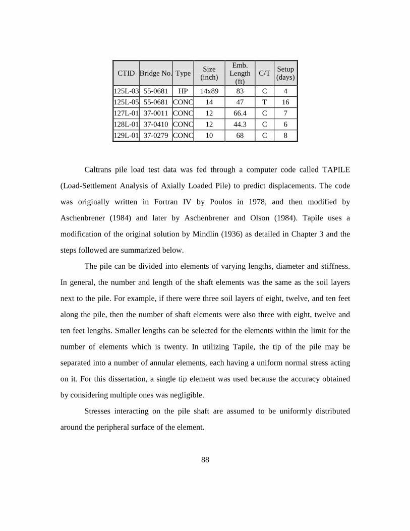
88


Emb. Length

(ft) C/T Setup

(days)

125L-03 55-0681 HP 14x89 83 C 4

125L-05 55-0681 CONC 14 47 T 16

127L-01 37-0011 CONC 12 66.4 C 7

128L-01 37-0410 CONC 12 44.3 C 6

129L-01 37-0279 CONC 10 68 C 8

Caltrans pile load test data was fed through a computer code called TAPILE

(Load-Settlement Analysis of Axially Loaded Pile) to predict displacements. The code

was originally written in Fortran IV by Poulos in 1978, and then modified by

Aschenbrener (1984) and later by Aschenbrener and Olson (1984). Tapile uses a

modification of the original solution by Mindlin (1936) as detailed in Chapter 3 and the

steps followed are summarized below.

The pile can be divided into elements of varying lengths, diameter and stiffness.

In general, the number and length of the shaft elements was the same as the soil layers

next to the pile. For example, if there were three soil layers of eight, twelve, and ten feet

along the pile, then the number of shaft elements were also three with eight, twelve and

ten feet lengths. Smaller lengths can be selected for the elements within the limit for the

number of elements which is twenty. In utilizing Tapile, the tip of the pile may be

separated into a number of annular elements, each having a uniform normal stress acting

on it. For this dissertation, a single tip element was used because the accuracy obtained

by considering multiple ones was negligible.

Stresses interacting on the pile shaft are assumed to be uniformly distributed

around the peripheral surface of the element.

89

Tapile uses an approximation for the heterogeneity of soils. The average soil

modulus is obtained by averaging the values next to the loaded element and the element

for which the displacement is being calculated.

Pile-soil slippage is allowed for by specifying limiting values of interface shear

stress at various elements along the pile. Different values of the limiting stresses for

compression and tension loading can be specified. Poisson’s ratio is assumed to remain

constant throughout the whole soil mass. Tapile conducts its analyses incrementally, in

which the specified increment of load is applied to the pile head and the resulting stress

and displacement increment at each element is evaluated and added to the corresponding

value at the previous load level. The program checks the computed pile-soil interface

stresses against the specified limiting values of soil shear strength. If the computed value

exceeds the limiting shear strength at any element, the side shear in for that element is set

equal to the shear strength of the soil. Then the soil-pile displacement compatibility

requirement is no longer valid and the soil can displace independently of the pile that it is

next to (“slippage”). The next load increment is applied and the procedure is repeated

until the specified number of load increments has been analyzed or all of the pile

elements reach their corresponding limiting values (pile capacity). For each load

increment, Tapile computes the stress and displacement at each element, the

displacement at the top of the pile and the distribution of axial load with depth along the

pile. The ultimate axial load capacity in compression and tension are also calculated

(Poulos, 1978).

A Visual Basic interface was used to create Tapile data files and to execute the

program for conducting analyses. The initial screen for input of data and subsequent

editing, and the summary table following an analysis (using the Run command in the

90

interface) are shown in Figures 4.1 and 4.2. An example of the data collected as part of

the Caltrans database is given in Figure 4.3, which also includes the matched soil

properties of layers along the pile length to obtain the measured pile capacity. Input and

output data files are included in Appendix C. A flow diagram of the steps involved in

Tapile calculations is presented in Figure 4.4.

Details of the displacement analyses based on the elastic method involving

Mindlin’s solution, laboratory and in-situ determination of input parameters, typical

recommended values given in literature, and further details of the pile load test database

used for analyses were provided in Chapter 3.

Figure 4.1 View of the pre-processing interface for Tapile program.

91

Figure 4.2 Tapile final screen in command window after execution.

In the following sections, results of analyses conducted using correlations

recommended in the literature are presented. Comparisons of calculated to measured

displacements are made graphically as well as statistically.

4.6 RESEARCH APPROACH

4.6.1 Failure Load Determination

It is imperative to estimate the ultimate pile capacity (failure load) as best as

possible in order to achieve success in determining the expected displacements. An error

in pile capacity will be reflected as an error in calculated displacements. Ideal pile

analysis thus would involve a concurrent investigation of capacity and displacement.

However, for an empirical study utilizing pile load tests, focus can be shifted from one to

the other because both the displacement and the capacity are known from pile load tests.

In this study, pile capacity is defined as the peak applied load as determined by pile load

testing (Figure 4.5a). The peak load is also employed in a single case where the pile is not

loaded to failure or there is no discernable failure load (Figure 4.5b).

92

Figu

re 4.3 A

n example of the collected pile load test data in

cohesive soil.

PILE LOAD TEST INFORMATIONCTID Bridge No. Bridge Name Bent No. Pile Number Pile Length Stick-up Pile Penetr. Loading SLTID

122L-01 22-0062 Mullen Overhead Bent 2R 21 51.20 0.00 51.20 Compression 736

Pile Diameter, D: 12 inch Pile Weight: 7.4 kips

Wall Thickness, t: 6 inch Qm,comp: 392.6 kipsVibrated? N Y or N Qm,tens: kips

Fvs: 1 Setup Time: 19 daysFvt: 1 DQF= 2 4REO

Pile Type: ConcretePile Shape: Square

Fp: 1 Equiv. Tip D: inch when roundTip Unit Capacity: 30.6 ksf Equiv. Tip D: 13.54 inch when square for area

Pile X Area: 144 sq. inch Equiv. Shaft D: 15.28 inch when square for circumferencePlug Area: 0.00 sq. inch Equiv. Tip D: inch when H for area

Tip Area: 144 sq. inch Equiv. Shaft D: inch when H for circumferenceEpile (ksi): 4500 H-Pile Surf. A: sq.ft/ft

Casing Depth (ft) Predrill Depth (ft) Relief Drill Depth (ft) Jetted Vibrated1.9

CAUTIONS 1

PILE CAPACITYK1 for E=K1*Su

K3 for ft=K3*Su

For fs=(25+K*N60),

K=

Adjust Side Shear

Rside = Tens/Comp

804 9.0

1.8 1.70 0.94K2 for E=K2*N

Es,t/Es,s

SOIL PROFILE Fine/Coarse? Equiv. N60/cu compression tension compr. compr. 1 compression tension

feet blows/foot ksf F 2.82 kPa ksf ksf ksf kPa ksf ksf kips kips

LayerNo Layer H N60 cu αααα Soil Type (N60 or cu)* L Side Es,s Tip Unit Capacity Tip Es,t Total Side Capacity1 1.9 0.01 sand 0.02 0.0 0.00 0.00 0 0.00 0.002 3.3 19 sand 62.7 0.0 0.00 0.00 0 0.00 0.003 26 2.42 0.44 clay 62.9 50.5 1.79 1.68 1946 186.2 175.14 1 2.42 0.44 clay 2.4 50.5 1.79 1.68 1946 7.2 6.75 19 3.4 0.38 clay 64.6 62.5 2.22 2.09 2734 1465.9 30.6 2734 168.6 158.5

2734

51.20OK

Notes:All dimensions in feet if not stated otherwise.Profile from FinalCT.dat (05/29/2005).First layer cased. Second layer is given as sand, but its contribution is not significant.

The general soil classification in FinalCT is clay. Fine SUM(cuL) 129.9 TOTAL 392.6 340.3

Assumed compression test. Coarse SUM(N60L) 62.7 compression tension

Minimum spacing unknown. Installed with Delmag D30 (54,250 ft-lb).

Side Shear

Load Test Readings

0.0

0.2

0.4

0.6

0.8

1.0

1.2

0 100 200 300 400 500

Load (kips)

Dis

pla

cem

ent (

inch

)

122L-01

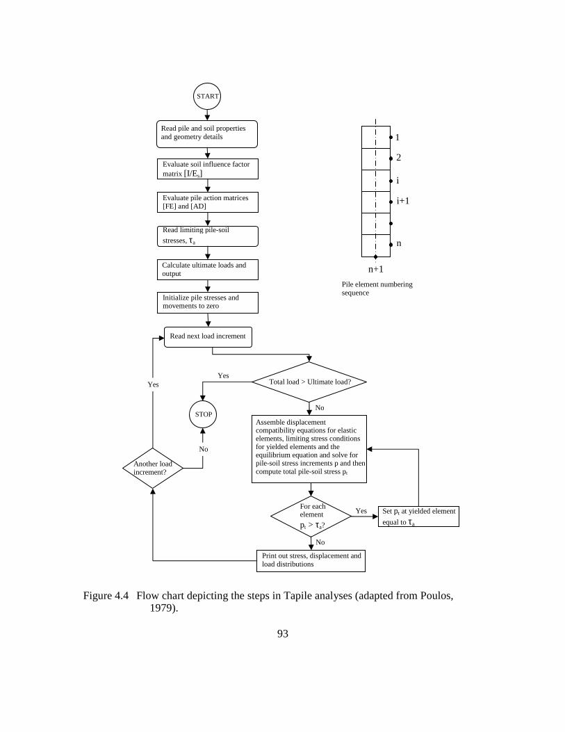
93

Figure 4.4 Flow chart depicting the steps in Tapile analyses (adapted from Poulos, 1979).

Read pile and soil properties and geometry details

Read next load increment

STOP

Another load increment?

Total load > Ultimate load?

No

Yes

Assemble displacement compatibility equations for elastic elements, limiting stress conditions for yielded elements and the equilibrium equation and solve for pile-soil stress increments p and then compute total pile-soil stress pt

For each element

pt > τa?

Yes

No

Print out stress, displacement and load distributions

Set pt at yielded element

equal to τa

Yes

No

Evaluate soil influence factor matrix [I/Es]

Evaluate pile action matrices [FE] and [AD]

Read limiting pile-soil

stresses, τa

Calculate ultimate loads and output

Initialize pile stresses and movements to zero

1

2

i

i+1

n

n+1

Pile element numbering sequence

START

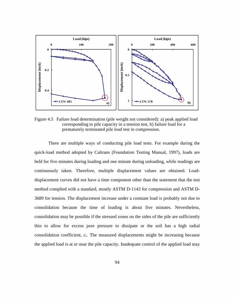
94

0

0.2

0.4

0 100 200

Load (kips)D

ispl

ace

men

t (in

ch)

LTN: 495 a)

0

0.5

1

0 200 400 600

Load (kips)

Dis

pla

cem

ent (

inch

)

LTN: 578 b)

Figure 4.5 Failure load determination (pile weight not considered): a) peak applied load corresponding to pile capacity in a tension test, b) failure load for a prematurely terminated pile load test in compression.

There are multiple ways of conducting pile load tests. For example during the

quick-load method adopted by Caltrans (Foundation Testing Manual, 1997), loads are

held for five minutes during loading and one minute during unloading, while readings are

continuously taken. Therefore, multiple displacement values are obtained. Load-

displacement curves did not have a time component other than the statement that the test

method complied with a standard, mostly ASTM D-1143 for compression and ASTM D-

3689 for tension. The displacement increase under a constant load is probably not due to

consolidation because the time of loading is about five minutes. Nevertheless,

consolidation may be possible if the stressed zones on the sides of the pile are sufficiently

thin to allow for excess pore pressure to dissipate or the soil has a high radial

consolidation coefficient, cr. The measured displacements might be increasing because

the applied load is at or near the pile capacity. Inadequate control of the applied load may

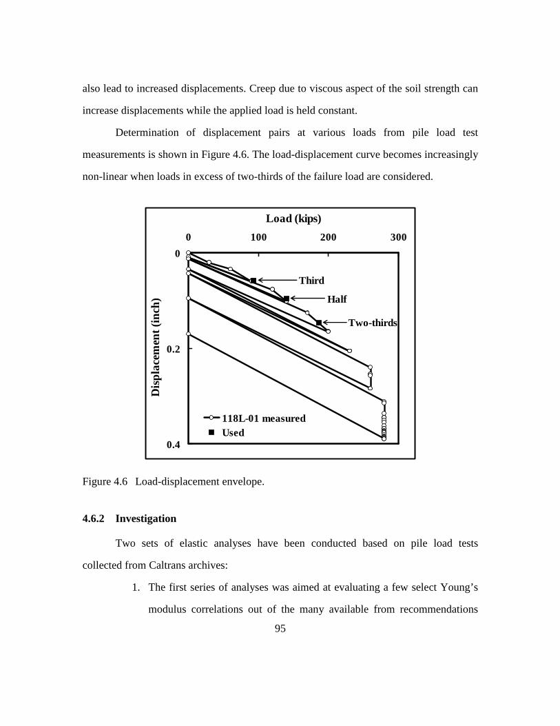
95

also lead to increased displacements. Creep due to viscous aspect of the soil strength can

increase displacements while the applied load is held constant.

Determination of displacement pairs at various loads from pile load test

measurements is shown in Figure 4.6. The load-displacement curve becomes increasingly

non-linear when loads in excess of two-thirds of the failure load are considered.

0

0.2

0.4

0 100 200 300

Load (kips)

Dis

plac

emen

t (in

ch)

118L-01 measuredUsed

Third

Half

Two-thirds

Figure 4.6 Load-displacement envelope.

4.6.2 Investigation

Two sets of elastic analyses have been conducted based on pile load tests

collected from Caltrans archives:

1. The first series of analyses was aimed at evaluating a few select Young’s

modulus correlations out of the many available from recommendations

96

found in literature to determine their relevance to pile displacement

calculations (Chapter 5).

2. The second set of analyses was an attempt towards establishing a

correlation for Young’s modulus that would improve the accuracy and

reliability of elastic analyses (Chapter 6).

The calculated and measured displacements have been compared graphically as

well as numerically to determine the “accuracy” of the suggested methods.

4.6.3 Graphical Evaluation

Calculated and measured displacements are compared graphically to observe

general trends and characteristics of the estimates employing recommended correlations

of Young’s modulus in the literature. The ratio of calculated displacements to the

measured displacements, (sc/sm), as well as the difference between displacements, (sc-sm),

is taken into consideration.

Separate plots are provided for each Young’s modulus correlation that has been

studied:

- cohesive soils: Aschenbrener (1984), Callanan and Kulhawy (1985),

Johnson (1986), and Poulos (1989) and (1972),

- cohesionless soils: Christoulas (1988), D’Appolonia et al. (1970), Decourt

et al. (1989), Denver (1982), Komornik (1974), Kurkur (1986), Shioi and

Fukui (1982), and Yamashita et al. (1987).

- mixed profiles (combination of cohesionless and cohesive soils):

Aschenbrener (1984), Poulos (1989), D’Appolonia et al. (1970),

Komornik (1974), Kurkur (1986), Shioi and Fukui (1982), and Yamashita

et al. (1987).

97

Direct estimations of pile displacements using the elastic compression/tension of a

free-standing column and Frank’s correlations with pile diameter are also shown in

graphs.

Negative values of displacements represent the displacements in a tension test and

positive numbers are for pile load tests in compression. These displacements are

presented on opposite axes in order to identify any possible differences due to loading

direction. A straight line depicting equality between calculated and measured

displacements is also plotted.

4.6.4 Statistical Evaluations

For analyses, the sample mean, ( x ), and the standard deviation, ( xs ), are used to

compare the estimated displacements utilizing the suggested correlations against those

observed in pile test results.

The accuracy of a method refers to how closely the calculated values can be used

to predict the measured values, which can be given by the arithmetic mean (average), of

the displacement ratio or displacement difference. The closer the estimated and measured

displacements match, the closer is the mean value of (x = sc / sm) to unity (=1). Similarly,

the better a measured displacement can be estimated, the closer will the mean value of (x

= sc – sm) be to zero. All of the equations below are given for the displacement ratio.

However, equations are valid for the displacement difference as well when appropriate

parameters are replaced.

The mean value of the displacement ratio is calculated as:

[ ]n

ii=1

1x x

n= ∑ .........................................................................................(4.7),

where, n is the number of pile load tests and i is a given pile load test.

98

Precision is the ability of a measurement to be reproduced consistently. The

standard deviation, σ indicates the plus-minus (±) scatter around the mean values. The

smaller the standard deviation, the greater is the reliability or precision of the estimation

method. The standard deviation of the displacement ratio is:

( )n

2 2x i

i=1

1s = x - x

n-1 ∑ .......................................................................(4.8).

In summary, a comparison can be made between correlations using the following

criteria: the better one would have a mean displacement ratio closer to one or a

displacement difference near zero, and a smaller standard deviation. These parameters

can then be ranked accordingly from most satisfactory to least or from best to worst. A

cumulative value can then be obtained to cross-evaluate the suggested correlations.

4.7 SUMMARY

In this chapter, the definitions of cohesive, cohesionless and mixed soil profiles

are given, as they are used throughout this dissertation. Caltrans database was divided

into three categories based on these descriptions. All of the analyses in the following

chapters rely on these subsets of data.

Various comparisons of calculated and measured displacements are made in the

next two chapters. Graphical and statistical evaluations of these comparisons are

explained in this chapter.

99

Chapter 5: Evaluation of Methods to Predict Axial Displacements

5.1 INTRODUCTION

In the literature, a large number of correlations for Young’s modulus have been

proposed, which are tied to various soil parameters obtained from laboratory or in-situ

measurements. In this chapter, a select few of these are introduced and used as part of the

elastic method to estimate displacements within the range of load ratios for which they

are recommended. The calculated and measured displacements are then compared.

Estimations that vary significantly from others in terms of displacement ratio (sc/sm) and

displacement difference (sc-sm) are identified. Factors are examined to determine their

respective effect on the outliers.

5.1.1 Direct Prediction of Displacement

An approximate prediction for displacements can be made with correlations

which are obtained empirically from past experience, relating a few parameters to pile

displacements via simple equations.

Frank (1985) suggested a correlation to estimate displacements based on his

experience with pressuremeter tests in France. He proposed the following range and

average value of displacements for piles under “working” loads, which he limited to half

of the determined maximum pile capacity:

0.008D ≤ ρ ≤ 0.012D ............................................................................(5.1),

with an average displacement of

ρaverage ≈ 0.009D ....................................................................................(5.2),

where, ρ: displacement and D: pile diameter.

100

Briaud and Tucker (1988) determined with a 95% probability that at a load ratio

of a half:

ρ ≤ 0.0125D ..........................................................................................(5.3).

Meyerhof (1959) earlier suggested a similar correlation for piles loaded up to a

third of their maximum capacity without regard to loading direction:

baseDρ=

30(FS).............................................................................................(5.4),

where, Dbase is the pile tip diameter and (FS) is the factor of safety, which he

recommended to be higher than three. The correlations proposed by Briaud and Tucker,

Frank, and Meyerhof are essentially the same for a factor of safety between three and

four. Poulos (1994) found that displacements calculated using Frank’s correlation to be

consistent with the displacements predicted by elastic method when “suitable” parameters

for stiffness of the soil are employed.

For convenience in this dissertation, 0.01D was employed in estimating

displacements of piles driven in all types of soils.

Another correlation commonly used for approximating displacements relies on

the elastic compression/tension of a free-standing column and ignores the effects of the

type of soil and the embedment on the distribution of the applied load along the pile:

pilepile,elastic

pile pile

PLρ =

A E................................................................................(5.5),

where, P: applied vertical load (kips), Lpile: length, Apile: cross-sectional area, and Epile:

modulus of elasticity of the pile. For a pile of known length, the value of

pile

pile pile

L

A E(inch/kips) is a constant for all applied loads, which is sometimes referred to as

the “compressibility of the pile”.

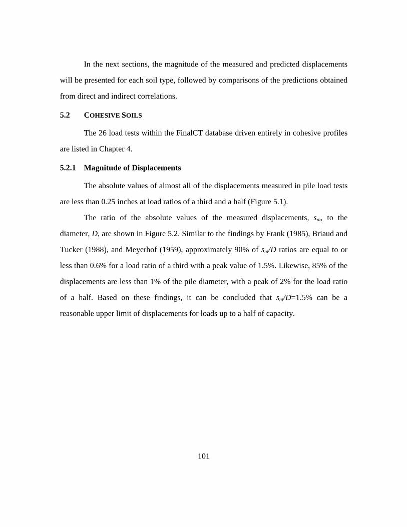
101

In the next sections, the magnitude of the measured and predicted displacements

will be presented for each soil type, followed by comparisons of the predictions obtained

from direct and indirect correlations.

5.2 COHESIVE SOILS

The 26 load tests within the FinalCT database driven entirely in cohesive profiles

are listed in Chapter 4.

5.2.1 Magnitude of Displacements

The absolute values of almost all of the displacements measured in pile load tests

are less than 0.25 inches at load ratios of a third and a half (Figure 5.1).

The ratio of the absolute values of the measured displacements, sm, to the

diameter, D, are shown in Figure 5.2. Similar to the findings by Frank (1985), Briaud and

Tucker (1988), and Meyerhof (1959), approximately 90% of sm/D ratios are equal to or

less than 0.6% for a load ratio of a third with a peak value of 1.5%. Likewise, 85% of the

displacements are less than 1% of the pile diameter, with a peak of 2% for the load ratio

of a half. Based on these findings, it can be concluded that sm/D=1.5% can be a

reasonable upper limit of displacements for loads up to a half of capacity.

102

0

6

12

-0.2 -0.1 0 0.1 0.2 0.3

D i s p l a c e m e n t ( i n c h )

N u

m b

e r

Third

Half

Figure 5.1 The magnitude of measured displacements, sm.

0

5

10

0.25 1.25 2.25

sm / D ( % )

N u

m b

e r

Third

Half

Figure 5.2 Measured displacements over pile diameter.

103

5.2.2 Correlations

Correlations of Young’s modulus selected from the literature with undrained

shear strength, cu, are listed in Table 5.1 and compared in Figure 5.3.

Table 5.1 Correlations of Young’s modulus with undrained shear strength, cu.

Pile Install. Es (ksf) Reference Notes/Method

Driven (300±100)cu Poulos (1989)* Back-calculated from pile load tests. Valid for third to half pile ultimate capacity.

Driven See below Poulos (1972) Equation derived by fitting the scanned graph. Valid for third to half ultimate capacity.

Bored See below Poulos (1972) Equation derived by fitting the scanned graph. Valid for third to half ultimate capacity.

Driven 800cu Aschenbrener (1984)/Aschenbrener and Olson (1984)*

Pile load test database (APC). Derived for half peak load applied to pile.

Driven 200cu Callanan & Kulhawy (1985), Johnson (1986)

Back-analysis of bored piles at half peak load(1985); matched laboratory strength to pressuremeter, CPT and plate bearing tests (1986)

Poulos (1972) (equations derived from fitting to scanned plots, cu in ksf) Es=-15.519cu

4+167.99cu3-207.11cu

2+257.37cu+58.374 (870 ksf max.) (driven piles) Es=140.54cu

4-610.45cu3+1024.8cu

2-623.88cu+196.75 (1750 ksf max.) (bored piles) * Used for piles in mixed profiles.

104

0

1

2

0 2 4Undrained Shear Strength, cu (ksf)

Yo

un

g's

Mo

du

lus

of S

oil,

E s (

ksf)x

103

Aschenbrener,1984 Poulos, 1989

Poulos, 1972driven

Poulos, 1972bored

Callanan & Kulhawy, 1985

Figure 5.3 Young’s modulus correlations with undrained shear strength.

Although all of the correlations are suggested for working loads, there is a

noticeable divergence among the calculated values for Young’s modulus. The variability

of undrained shear strength was discussed in Chapter 3. Aschenbrener (1984) and

Aschenbrener and Olson (1984) utilized Davisson’s (1972) formula for determining pile

capacity from a load-displacement curve, which corresponds to the load on the curve

intersected at the following displacement value (Figure 5.4):

f bp p

QLS = + 0.15"+ 0.01D

A E (pile loaded in compression).................. (5.6)

fp p

QLS = 0.15"

A E− − (pile loaded in tension)........................................(5.7)

105

where, Q is applied load, L is the total length, Ap is the cross-sectional area, Ep is Young's

modulus, and Db is the base diameter of the pile. Such a determination of failure load

may lead to lower peak loads than those which other researchers utilized for their

correlations. The smaller displacements predicted from Aschenbrener’s suggestion may

be explained by matching smaller displacements at lower loads (Figure 5.4).

0

0.5

1

0 100 200

Load (kips)

Dis

pla

cem

ent (

inch

)

Measured

167

173

Davisson line

Figure 5.4 Difference between calculated pile capacities: Davisson (167 kips) versus peak applied load (173 kips).

5.2.3 Measurements versus Predictions

A comparison of the measured displacements versus predicted displacements

using the correlation suggested by Poulos (1989) indicates good overall agreement and is

representative of the outcome from other correlations (Figure 5.5) for a load ratio up to a

half. All of absolute values of the measured and predicted displacements are less than the

0.5 inches. There is a tendency to predict larger displacements than those measured for all

but one (Aschenbrener, 1984) of the correlations. A larger dispersion of the

106

displacements can be seen at a load ratio of a half. For all of the predictions, the loading

direction, i.e., tension versus compression, does not appear to have an effect on the

magnitude or error of predicted displacements.

Outliers, marked with their respective load test numbers (LTNs) in Table 5.5, are

discussed in section 5.2.6.

Poulos, 1989

0

0.4

-0.4 0 0.4

sm ( i n c h )

|sc|

( i n

c h

)

ThirdHalfsc=sm

COMP.TENSION

666

652

413

448

Figure 5.5 Comparison of measured and predicted displacements.

5.2.4 Displacement Ratio, sc/sm

The average and standard deviation of the displacement ratio for all investigated

correlations at load ratios up to a half are given in Table 5.2 and shown in Figure 5.6.

Predictions can be ranked from one (best) to seven (worst) based on their relative

performances (Table 5.3). An overall conclusion on the best correlation may be obtained

by looking at rankings from both load ratios. The absolute difference of the displacement

ratios from sc/sm = 1 is calculated to rank the mean values.

107

The top four predictive methods based on the rankings at both load ratios are as

follows: elastic column, Aschenbrener (1984), Poulos (1989), and Poulos (1972, driven

piles). These findings coincide with conclusions reached by a visual inspection of the

displacements.

Table 5.2 The statistics of displacement ratio (sc/sm) (N = 26).

Load Ratio Value Poulos

(1989)

Poulos (1972)

(driven)

Poulos (1972) (bored)

Aschenbre-ner (1984)

Callanan/ Kulhawy

1985; Johnson

1986

Frank 1985

Elastic column

Mean, x 1.76 1.81 3.09 1.15 2.44 3.25 1.63 ⅓

Stand. Dev., sx 1.14 1.33 2.70 1.18 1.68 2.54 0.64 Mean, x 1.42 1.46 2.49 0.89 1.97 1.77 1.36 ½ Stand. Dev., sx 0.67 0.80 1.69 0.61 1.00 1.22 0.41

0

2

4

Po

ulo

s 1

98

9

Po

ulo

s 1

97

2dr

iven

Po

ulo

s 1

97

2bo

red

Asc

henb

rene

r1

98

4C

alla

nan

&K

ulha

wy

Fra

nk 1

98

5

Ela

stic

colu

mn

M e

a n

( s

c / s

m )

1/3 1/20

1

2

3

Po

ulo

s 1

98

9

Po

ulo

s 1

97

2dr

iven

Po

ulo

s 1

97

2bo

red

Asc

henb

rene

r1

98

4C

alla

nan

&K

ulha

wy

Fra

nk 1

98

5

Ela

stic

colu

mn

S t

d. d

e v

. ( s

c / s

m )

1/3 1/2

Figure 5.6 Comparison of correlations based on mean and standard deviation of displacement ratio (sc/sm).

108

Table 5.3 Ranking of correlations based on displacement ratio (sc/sm).


(1989)

Poulos (1972)

(driven)



Callanan/ Kulhawy

1985; Johnson

1986

Frank 1985

Elastic column

Mean1, x 3 4 6 1 5 7 2 ⅓

Stand. Dev., sx 2 4 7 3 5 6 1 Mean, x 3 4 7 1 6 5 2 ½ Stand. Dev., sx 3 4 7 2 5 6 1

1 Absolute difference from (sc/sm) = 1 used for ranking mean values.

Three correlations of Young’s modulus result in much larger errors in terms of

displacement ratios: Callanan and Kulhawy (1985)/Johnson (1986), Poulos (1972, bored

pile) and Frank (1985) (Figure 5.6). Poulos (1972) especially leads to higher predicted

displacements than those measured in pile load tests. The correlation of Callanan and

Kulhawy and Poulos are derived from the results of load tests on bored piles, which

typically require larger displacements than driven piles to mobilize their full side and tip

capacity. Thus, both tend to overestimate displacements for driven piles. Frank’s method,

on the other hand, takes only the diameter of the pile into consideration and has a large

variability when compared against measured displacements.

5.2.5 Displacement Difference, sc-sm

Differences in displacements are useful in evaluating a method, especially when

small displacements are considered. Even a minor error in prediction may cause a large

displacement ratio to be calculated although the differences may actually be trivial.

Average and standard deviation of the displacement differences are tabulated in

Table 5.4 and shown in Figure 5.7. The mean values of displacement differences for each

prediction are not large and the standard deviation does not change significantly for

109

increased loading. Based on the averages of displacement differences, all of the

correlations perform reasonably well and close to each other in terms of average values

and standard deviations. Hence, rankings would not necessarily reflect actual superiority

of any correlation, and therefore, are not presented. However, it should be noted that the

three correlations (Poulos, 1972 bored; Callanan and Kulhawy, 1985/Johnson, 1986; and

Frank, 1985) that resulted in high displacement ratios do not have high displacement

differences on an average; however their standard deviations the three highest among all

of the correlations that were considered. The reason for average differences that are close

to zero is the existence of similarly high positive and negative values.

Table 5.4 The statistics for displacement differences (sc-sm) (inch) (N = 26).

Load Ratio Parameter Poulos,

(1989)

Poulos, (1972)

(driven)

Poulos, (1972) (bored)

Aschenbre-ner, (1984)

Callanan/ Kulhawy,

1985; Johnson,

1986

Frank, 1985

Elastic column

Mean, x -0.01 -0.01 -0.01 -0.02 -0.01 0.00 0.00 ⅓ Stand.

Dev., sx 0.05 0.06 0.12 0.05 0.08 0.13 0.05

Mean, x 0.02 0.02 0.06 0.02 0.04 0.06 0.03 ½ Stand.

Dev., sx 0.04 0.05 0.09 0.05 0.06 0.09 0.04

110

-0.05

0

0.05

0.1

Po

ulo

s 1

989

Po

ulo

s 1

972

driv

enP

ou

los

197

2b

ored

Asc

hen

bre

ner

198

4C

alla

na

n &

Ku

lha

wy

Fra

nk

1985

Ela

stic

colu

mn

M e

a n

( s

c -

s m

)

1/3 1/20

0.05

0.1

0.15

Pou

los

19

89

Pou

los

19

72d

riven

Pou

los

19

72b

ore

dA

sch

enb

ren

er1

984

Cal

lan

an &

Ku

lha

wy

Fra

nk

198

5

Ela

stic

colu

mn

S t

d. d

e v

. ( s

c -

s m

)

1/3 1/2

Figure 5.7 Comparison of correlations based on mean and standard deviation of displacement differences (sc-sm) (both in inches).

5.2.6 Outliers

Within the context of this dissertation, an outlier is defined as a prediction that

deviates significantly from the displacement equality line (sc = sm) and can be ascertained

by having both of the following properties:

1) a displacement ratio (sc/sm) that has an absolute error in excess of 20%, i.e.,

0.80sm ≥ sc or sc ≥ 1.2sm; as well as

2) an absolute displacement difference c m(s -s ) larger than 0.1 inches.

Of these two criteria, the displacement difference is more influential than the

displacement ratio in determining outliers.

Four tests (one high and three low in terms of sc/sm) consistently produce outliers

for most, if not all, of the correlations and load ratios of up to a half (Table 5.5 and shown

with larger symbols in Figure 5.5). They are investigated in further detail to identify

properties which may explain the larger discrepancy.

111

Table 5.5 Comparison of predicted and measured displacements for outliers.

Load Test

Number (LTN)

Load Ratio

Displ. Ratio

or Diff.

(inch)

Poulos (1989)

Poulos (1972)

(driven)



Callanan/ Kulhawy

1985; Johnson

1986

Frank 1985

Elastic column

sc/sm 0.58† 0.68 0.46 0.32 0.80 1.85 1.01 ⅓ |sc–sm| 0.05 0.04 0.07 0.09 0.03 0.11 0 sc/sm 0.48 0.56 0.38 0.26 0.66 1.01 0.83

413 ½

|sc–sm| 0.12 0.10 0.15 0.18 0.08 0 0.04 sc/sm 5.69 6.49 12.94 6.01 8.46 11.09 2.83

⅓ |sc–sm| 0.10 0.12 0.26 0.11 0.16 0.22 0.04 sc/sm 3.05 3.48 6.93 3.22 4.54 3.96 1.52

448 ½

|sc–sm| 0.12 0.15 0.36 0.13 0.21 0.18 0.03 sc/sm 0.52 0.49 0.80 0.29 0.74 0.92 0.86

⅓ |sc–sm| 0.10 0.10 0.04 0.13 0.07 0.07 0.09 sc/sm 0.60 0.59 0.91 0.41 0.77 0.49 0.65

652 ½

|sc–sm| 0.11 0.12 0.03 0.17 0.06 0.14 0.10 sc/sm 0.52 0.49 0.86 0.29 0.74 0.92 0.86

⅓ |sc–sm| 0.08 0.09 0.02 0.12 0.05 0.01 0.02 sc/sm 0.43 0.40 0.71 0.24 0.60 0.50 0.71

666 ½

|sc–sm| 0.18 0.19 0.09 0.25 0.13 0.16 0.09 † Outliers are bold-faced and italicized

The following factors are investigated for the outliers: 1) soil layering, 2) total

length (L), 3) diameter (D), 4) L/D ratio, and 5) stiffness (ApEp/L, where Ap is cross-

sectional area and Ep is Young’s modulus of pile).

Relevant information from the FinalCT database for the load tests, including soil

layering along the length of the pile, is presented in Table 5.6. The first pile (LTN: 413)

was driven into a soil profile with three layers of sand constituting 8% of the side area of

the pile and 9% of the total capacity. Three of the four piles were driven through a larger

casing at the top.

The distribution of the pile diameter versus sc/sm is presented for predictions made

using Poulos’ (1989) correlation, which exemplifies the outcome of all correlations and

of the other three parameters considered (Figure 5.8). The range of values for all piles

112

driven in cohesive soils is compared to that for outliers in Table 5.7. None of the

investigated parameters provides a clear explanation for the outliers.

Table 5.6 Details of pile load tests that have been investigated further.

LTN Type Sect. C/T L DR AE/L W D Qf Sfail Setup Layer Soil h cu/N

413 STLP CIRC T 75.5 1.04 1184 9.5 24 4551.48 14 1 Clay 4 0.3 2 Clay 15 1.77 3 Sand 3 29 4 Clay 25 3.15 5 Sand 2 23 6 Clay 4 2.54 7 Sand 1 20 8 Clay 12.5 3.81

LTN Type Sect. C/T L DR AE/L W D Qf Sfail Setup Layer Soil h cu/N 448 STLP CIRC T 92.7 0.12 1324 40.7 24 2030.87 35 1 Clay 4.3 0.9

2 Clay 5 0.63 3 Clay 5 0.51 4 Clay 5 0.74 5 Clay 15 0.53 6 Clay 10 0.58 7 Clay 25 0.81 8 Clay 9.7 0.87

LTN Type Sect. C/T L DR AE/L W D Qf Sfail Setup Layer Soil h cu/N 652 CONC SQRE C 105.5 1 674 22.3 14 2720.72 N/A 1 Clay 25 0.65

2 Clay 40 1.5 3 Clay 15 1 4 Clay 5.5 2

LTN Type Sect. C/T L DR AE/L W D Qf Sfail Setup Layer Soil h cu/N 666 STLP CIRC C 85 0.12 693 9.2 16 3231.67 1553 1 Clay 82.1 0.33

2 Clay 2.9 1.5 LTN : Load test number (arbitrary number identifying the test) Type : Pile type (CONC: concrete, STLP: steel pipe pile, HPIL: H-pile etc.) Sect. : Pile cross-section (SQRE: square, CIRC: circular etc.) C/T : Pile load test direction: tension (T) or compression (C) L : Length of pile penetrated in soil (feet) DR : Displacement ratio (1 for solid pile, >1 for oversized cover plates) AE/L : Pile spring constant, stiffness (kips/inch) W : Weight of pile submerged in soil (kips) D : Pile diameter (inch) Qf : Plunging failure load (kips) Sfail : Displacement at plunging load (inch) Setup : Set up time, time from end of driving to start of test, N/A if not known (days)

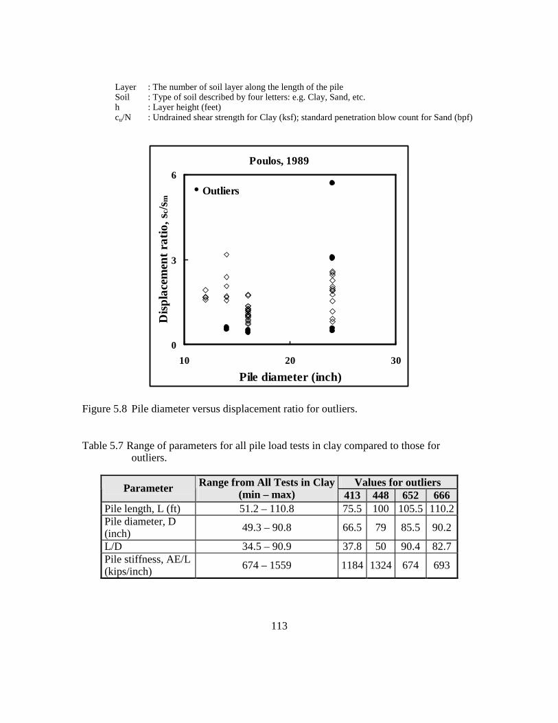
113

Layer : The number of soil layer along the length of the pile Soil : Type of soil described by four letters: e.g. Clay, Sand, etc. h : Layer height (feet) cu/N : Undrained shear strength for Clay (ksf); standard penetration blow count for Sand (bpf)

Poulos, 1989

0

3

6

10 20 30

Pile diameter (inch)

Dis

pla

cem

ent

ratio

, sc/s

m

• Outliers

Figure 5.8 Pile diameter versus displacement ratio for outliers.

Table 5.7 Range of parameters for all pile load tests in clay compared to those for outliers.

Values for outliers Parameter Range from All Tests in Clay (min – max) 413 448 652 666

Pile length, L (ft) 51.2 – 110.8 75.5 100 105.5 110.2 Pile diameter, D (inch)

49.3 – 90.8 66.5 79 85.5 90.2

L/D 34.5 – 90.9 37.8 50 90.4 82.7 Pile stiffness, AE/L (kips/inch)

674 – 1559 1184 1324 674 693

114

5.3 COHESIONLESS SOILS

Thirty-four load tests driven into cohesionless soils were investigated (see

Chapter 4 for details).


For load ratios up to a half, all of the measured displacements are less than 0.5

inches (Figure 5.9).

Magnitude of measured displacements

0

5

10

15

-0.3 -0.1 0.1 0.3 0.5

Displacement (inch)

Nu

mb

er

Third

Half

Figure 5.9 The magnitude of measured displacements for load ratios up to a half.

The sm/D ratios are presented in Figure 5.10 for load ratios of a third and a half.

For a load ratio of a third, all but one of the measurements are less than 1.5% of the pile

diameter. However, for a load ratio of a half, approximately 25% of the measurements

are larger than 1.5% of the pile diameter.

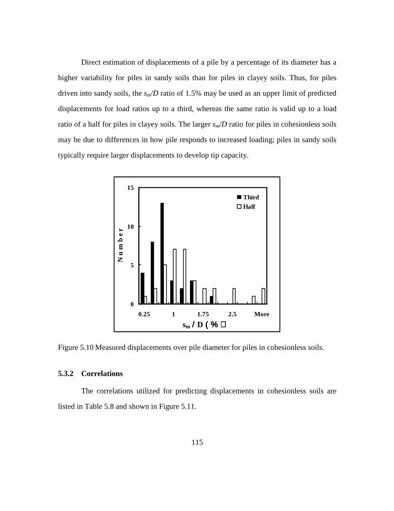
115

Direct estimation of displacements of a pile by a percentage of its diameter has a

higher variability for piles in sandy soils than for piles in clayey soils. Thus, for piles

driven into sandy soils, the sm/D ratio of 1.5% may be used as an upper limit of predicted

displacements for load ratios up to a third, whereas the same ratio is valid up to a load

ratio of a half for piles in clayey soils. The larger sm/D ratio for piles in cohesionless soils

may be due to differences in how pile responds to increased loading; piles in sandy soils

typically require larger displacements to develop tip capacity.

0

5

10

15

0.25 1 1.75 2.5 More

sm / / / / D ( % ) ( % ) ( % ) ( % )

N u

m b

e r

Third

Half

Figure 5.10 Measured displacements over pile diameter for piles in cohesionless soils.

5.3.2 Correlations

The correlations utilized for predicting displacements in cohesionless soils are

listed in Table 5.8 and shown in Figure 5.11.

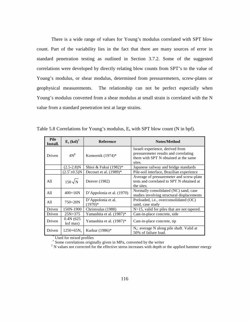
116

There is a wide range of values for Young’s modulus correlated with SPT blow

count. Part of the variability lies in the fact that there are many sources of error in

standard penetration testing as outlined in Section 3.7.2. Some of the suggested

correlations were developed by directly relating blow counts from SPT’s to the value of

Young’s modulus, or shear modulus, determined from pressuremeters, screw-plates or

geophysical measurements. The relationship can not be perfect especially when

Young’s modulus converted from a shear modulus at small strain is correlated with the N

value from a standard penetration test at large strains.

Table 5.8 Correlations for Young’s modulus, Es with SPT blow count (N in bpf).

Pile Install. Es (ksf)† Reference Notes/Method

Driven 4N‡ Komornik (1974)*

Israeli experience, derived from pressuremeter results and correlating them with SPT N obtained at the same sites.

(2.5-2.8)N Shioi & Fukui (1982)* Japanese railway and bridge standards (2.5†±0.5)N Decourt et al. (1989)* Pile-soil interface, Brazilian experience

All 150 N Denver (1982) Average of pressuremeter and screw-plate tests and correlated to SPT N obtained at the sites.

All 400+16N D’Appolonia et al. (1970) Normally consolidated (NC) sand, case studies involving structural displacements

All 750+20N D’Appolonia et al. (1970)*

Preloaded, i.e., overconsolidated (OC) sand, case study

Driven 150N-1900 Christoulas (1988) N>15, valid for piles that are not tapered. Driven 25N+375 Yamashita et al. (1987)* Cast-in-place concrete, side

Driven 0.4N (625 ksf max) Yamashita et al. (1987)* Cast-in-place concrete, tip

Driven 1250+65Ns Kurkur (1986)* Ns: average N along pile shaft. Valid at 50% of failure load.

* Used for mixed profiles

† Some correlations originally given in MPa, converted by the writer ‡ N values not corrected for the effective stress increases with depth or the applied hammer energy

117

0

2

4

0 25 50SPT N60 (bpf)

Es

(ksf

) x1

03

Shioi&Fukui1982

Christoulas, 1988

Denver, 1982

D'Appolonia et al.,1970, OC

Komornik, 1974

D'Appolonia etal., 1970, NC

Yamashita,1987

Figure 5.11 Correlations of SPT blow count with Young’s modulus of soil.

5.3.3 Predictions versus Measurement

A comparison of measured displacements with those predicted using Komornik’s

(1974) correlation, for a load ratio up to a half, are shown in Figure 5.12. Overall, the

measured and calculated displacements agree well with each other and are, for the most

part, similar to the outcome obtained from the other correlations that were investigated.

The absolute values of the displacements are less than 0.5 inches. The direction of

the pile loading does not seem to have an effect on the predicted displacements in terms

of the errors observed. Displacements estimated at a load ratio of a third conform better

to the measured displacements than those at a load ratio of a half. There is an overall

tendency to predict smaller displacements than those measured in pile load tests. The

118

only exception is obtained from the elastic column approach, which generally suggests

higher displacements than the measured ones.

Only the outliers for a load ratio of a half are marked in Figure 5.12 to avoid

clutter. Further discussion of these pile load tests is provided in section 5.3.6.

Komornik, 1974

0

0.5

-0.5 0 0.5

s m ( i n c h )

s c (

i n

c h

)

ThirdHalfsc=sm

572

578609

580577581

573

781

782

576

TENS. COMP.

Figure 5.12 Measured and predicted displacements for piles in sandy soils.


The mean and standard deviation of the displacement ratio for all investigated

correlations loaded up to a load ratio of a half are listed in Table 5.9 and shown in Figure

5.13.

Predictions using the correlation suggested by Christoulas (1988) have a high

mean with a large scatter. Therefore, his method is excluded from further comparisons.

Unlike the correlations for clayey soils, the ranking of correlations for sandy soils

does not point toward a specific correlation that works for load ratios of a third and a half

(Table 5.10). For example, the predictions using Komornik’s correlation are most

119

accurate for the load ratio of a third. However, its ranking drops to sixth when a load ratio

of a half is considered.

Kurkur’s predictions have the smallest standard deviation for both load ratios,

which may be due to the single averaged value of SPT N utilized for all soil layers, based

on their thicknesses, which prevents errors that may occur when the properties of layers

vary significantly.

Table 5.9 Mean and standard deviation for correlations (N = 34).

Load RatioValue

Komor-nik, 1974

Shioi/ Fukui, 1982;

Decourt, 1989

Den-ver, 1982

D’Appo-lonia et

al., 1970 (NC)

D’Appo-lonia et

al., 1970 (OC)

Chris-toulas, 1988

Yamas-hita et

al., 1987

Kur-kur, 1986

Frank, 1985

Elastic column

Mean,x 0.97 1.26 1.86 1.62 1.19 18.19 1.16 0.79 2.74 1.24 ⅓ St.

Dev., sx 0.58 0.80 1.23 1.16 0.75 91.96 0.71 0.48 2.88 0.62

Mean,x 0.74 0.96 1.43 1.26 0.90 16.92 0.88 0.62 0.94 0.93 ½ St.

Dev., sx 0.42 0.61 0.91 0.75 0.50 87.24 0.49 0.35 1.19 0.42

0

1

2

3

Kom

orn

ik1

974

Sh

ioi &

Fu

kui 1

982

Den

ver

198

2D

'Ap

po

lon

ia19

70 (

NC

)D

'Ap

po

lon

ia1

970

(OC

)Y

ama

shita

19

87K

urk

ur

1986

Fra

nk

198

5

Ela

stic

colu

mn

M e

a n

(s

c / s

m ) 1/3 1/2

0

1

2

3

Ko

mor

nik

197

4S

hio

i &F

uku

i 19

82

Den

ver

1982

D'A

pp

olo

nia

197

0 (N

C)

D'A

pp

olo

nia

19

70 (

OC

)Y

am

ash

ita19

87

Ku

rku

r1

986

Fra

nk

198

5

Ela

stic

colu

mn

S t

d. d

e v

. ( s

c / s

m )

1/3 1/2

Figure 5.13 Comparison of correlations based on mean and standard deviation of displacement ratio (sc/sm).

120

Table 5.10 Rankings corresponding to each correlation.

Load Ratio Value

Komor-nik, 1974

Shioi/ Fukui, 1982;

Decourt, 1989

Den-ver, 1982

D’Appo-lonia et

al., 1970 (NC)

D’Appo-lonia et

al., 1970 (OC)

Yamas-hita et

al., 1987

Kur-kur, 1986

Frank, 1985

Elastic column

Mean,x 1 6 8 7 3 2 4 9 5 ⅓ St.

Dev., sx 2 6 8 7 5 4 1 9 3

Mean,x 7 1 9 6 3 4 8 5 2 ½ St.

Dev., sx 3 6 9 7 5 4 1 8 2


The mean and standard deviation of displacement differences for all of the

investigated methods vary within a narrow margin at load ratios of a third and a half

(Table 5.11 and Figure 5.14).

Seven out of nine methods have positive displacement differences, i.e., the

calculated displacements are higher than the ones that are measured. Although the scatter

increases when a load ratio of a half is considered, displacement differences remain

approximately constant. The ranking of displacement differences is of little value because

the outcomes are similar.

The correlations produce acceptable results as far as the differences between

predicted and measured displacements at working loads are concerned.

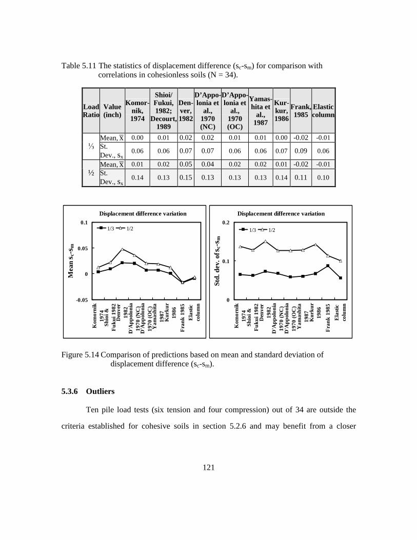
121

Table 5.11 The statistics of displacement difference (sc-sm) for comparison with correlations in cohesionless soils (N = 34).

Load Ratio

Value (inch)

Komor-nik, 1974

Shioi/ Fukui, 1982;

Decourt, 1989

Den-ver, 1982

D’Appo-lonia et

al., 1970 (NC)

D’Appo-lonia et

al., 1970 (OC)

Yamas-hita et

al., 1987

Kur-kur, 1986

Frank, 1985

Elastic column

Mean,x 0.00 0.01 0.02 0.02 0.01 0.01 0.00 -0.02 -0.01 ⅓ St.

Dev., sx 0.06 0.06 0.07 0.07 0.06 0.06 0.07 0.09 0.06

Mean,x 0.01 0.02 0.05 0.04 0.02 0.02 0.01 -0.02 -0.01 ½ St.

Dev., sx 0.14 0.13 0.15 0.13 0.13 0.13 0.14 0.11 0.10

Displacement difference variation

-0.05

0

0.05

0.1

Kom

orn

ik19

74

Sh

ioi &

Fu

kui 1

982

Den

ver

19

82D

'Ap

pol

on

ia19

70

(NC

)D

'Ap

pol

on

ia1

970

(O

C)

Ya

mas

hita

1987

Ku

rku

r19

86

Fra

nk

198

5

Ela

stic

colu

mn

Mea

n s c

-sm

1/3 1/2

Displacement difference variation

0

0.1

0.2

Kom

orn

ik19

74

Sh

ioi &

Fu

kui 1

982

Den

ver

19

82D

'Ap

pol

on

ia19

70

(NC

)D

'Ap

pol

on

ia1

970

(O

C)

Ya

mas

hita

1987

Ku

rku

r19

86

Fra

nk

198

5

Ela

stic

colu

mn

Std

. dev

. of s

c-s m

1/3 1/2

Figure 5.14 Comparison of predictions based on mean and standard deviation of displacement difference (sc-sm).

5.3.6 Outliers

Ten pile load tests (six tension and four compression) out of 34 are outside the

criteria established for cohesive soils in section 5.2.6 and may benefit from a closer

122

investigation (Table 5.12). Other relevant information for each pile load test, including

the soil layering, is presented in Table 5.13.

Table 5.12 Displacement ratio and difference for outliers.

Load Test

Number (LTN)

Load Ratio

Displ. Ratio

or Diff.

(inch)

Komor-nik, 1974

Shioi/ Fukui, 1982;

Decourt, 1989

Den-ver, 1982

D’Appo-lonia et

al., 1970 (NC)

D’Appo-lonia et

al., 1970 (OC)

Yamas-hita et

al., 1987

Kur-kur, 1986

Frank, 1985

Elastic column

sc/sm 0.45† 0.56 0.81 0.75 0.57 0.54 0.41 1.27 2.13 ⅓

|sc–sm| 0.07 0.06 0.02 0.03 0.05 0.06 0.07 -0.03 -0.14 sc/sm 0.33 0.41 0.60 0.55 0.42 0.40 0.30 0.62 1.56

572 ½

|sc–sm| 0.17 0.15 0.10 0.12 0.15 0.15 0.18 0.10 -0.14 sc/sm 0.57 0.71 1.00 0.92 0.70 0.68 0.53 1.67 2.76

⅓ |sc–sm| 0.04 0.02 0.00 0.01 0.02 0.03 0.04 -0.06 -0.15 sc/sm 0.43 0.53 0.74 0.68 0.52 0.50 0.40 0.82 2.05

573 ½

|sc–sm| 0.10 0.08 0.04 0.05 0.08 0.08 0.10 0.03 -0.18 sc/sm 0.34 0.40 0.61 0.55 0.43 0.40 0.32 0.56 1.41

⅓ |sc–sm| -0.19 -0.17 -0.11 -0.13 -0.16 -0.17 -0.20 -0.13 0.12 sc/sm 0.32 0.38 0.58 0.52 0.41 0.38 0.32 0.35 1.33

576 ½

|sc–sm| -0.31 -0.28 -0.19 -0.22 -0.27 -0.28 -0.31 -0.30 0.15 sc/sm 0.26 0.31 0.47 0.43 0.33 0.31 0.24 0.74 1.09

⅓ |sc–sm| 0.16 0.15 0.12 0.12 0.15 0.15 0.17 0.06 -0.02 sc/sm 0.23 0.27 0.41 0.37 0.29 0.27 0.22 0.43 0.96

577 ½

|sc–sm| 0.28 0.27 0.22 0.23 0.26 0.27 0.29 0.21 0.02 sc/sm 0.25 0.32 0.50 0.45 0.32 0.31 0.20 0.97 1.71

⅓ |sc–sm| 0.12 0.11 0.08 0.09 0.11 0.11 0.13 0.01 -0.12 sc/sm 0.21 0.27 0.42 0.38 0.27 0.26 0.18 0.53 1.42

578 ½

|sc–sm| 0.24 0.22 0.18 0.19 0.22 0.22 0.25 0.14 -0.13 sc/sm 0.35 0.42 0.61 0.57 0.43 0.41 0.31 0.67 1.38

⅓ |sc–sm| -0.14 -0.12 -0.08 -0.09 -0.12 -0.12 -0.15 -0.07 0.08 sc/sm 0.33 0.40 0.58 0.54 0.41 0.39 0.31 0.42 1.31

580 ½

|sc–sm| -0.22 -0.20 -0.14 -0.15 -0.19 -0.20 -0.23 -0.19 0.10 sc/sm 0.30 0.36 0.53 0.49 0.38 0.36 0.26 1.04 1.20

⅓ |sc–sm| 0.09 0.09 0.06 0.07 0.08 0.09 0.10 -0.01 -0.03 sc/sm 0.25 0.30 0.44 0.41 0.31 0.30 0.23 0.58 0.99

581 ½

|sc–sm| 0.18 0.17 0.14 0.14 0.17 0.17 0.19 0.10 0.00 sc/sm 0.38 0.44 0.73 0.64 0.46 0.45 0.27 1.26 0.59

⅓ |sc–sm| 0.09 0.08 0.04 0.05 0.08 0.08 0.11 -0.04 0.06 sc/sm 0.23 0.27 0.43 0.38 0.28 0.27 0.18 0.49 0.34

609 ½

|sc–sm| 0.29 0.28 0.22 0.24 0.27 0.28 0.31 0.19 0.25 sc/sm 0.51 0.74 1.04 0.93 0.59 0.63 0.38 1.93 0.87 781

⅓ |sc–sm| -0.03 -0.02 0.00 0.00 -0.03 -0.02 -0.04 0.06 -0.01

123

Load Test

Number (LTN)

Load Ratio

Displ. Ratio

or Diff.

(inch)

Komor-nik, 1974

Shioi/ Fukui, 1982;

Decourt, 1989

Den-ver, 1982

D’Appo-lonia et

al., 1970 (NC)

D’Appo-lonia et

al., 1970 (OC)

Yamas-hita et

al., 1987

Kur-kur, 1986

Frank, 1985

Elastic column

sc/sm 0.31 0.45 0.63 0.56 0.36 0.38 0.23 0.78 0.52 ½ |sc–sm| -0.11 -0.09 -0.06 -0.07 -0.10 -0.10 -0.12 -0.03 -0.07 sc/sm 0.30 0.44 0.62 0.55 0.35 0.37 0.23 1.37 0.50

⅓ |sc–sm| -0.06 -0.05 -0.03 -0.04 -0.06 -0.06 -0.07 0.03 -0.04

sc/sm 0.10 0.14 0.20 0.18 0.11 0.12 0.07 0.29 0.16 782

½ |sc–sm| -0.37 -0.35 -0.33 -0.33 -0.36 -0.36 -0.38 -0.29 -0.34

† Outliers are given in bold and italics.

Table 5.13 Properties and soil layering for outlying pile load tests.

LTN Type Sect. C/T L DR AE/L W D Qf Sfail Setup Layer Soil h N 572 STLP CIRC T 91.1 0.12 610 12.8 16 476 1.32 6 1 SaSi 6.5 25

2 SaSi 15 15 3 Sand 5 20 4 Sand 21.5 8 5 Sand 6.5 8 6 Sand 8 14 7 Sand 11 24 8 Sand 7 18 9 Sand 5 34 10 Sand 5.6 55

LTN Type Sect. C/T L DR AE/L W D Qf Sfail Setup Layer Soil h N 573 STLP CIRC T 85.0 0.12 499 7.6 14 341 1.62 7 1 SaSi 6.5 25

2 SaSi 15 15 3 Sand 5 20 4 Sand 21.5 8 5 Sand 6.5 8 6 Sand 8 14 7 Sand 11 24 8 Sand 7 18 9 Sand 4.5 34

LTN Type Sect. C/T L DR AE/L W D Qf Sfail Setup Layer Soil h N 576 STLP CIRC C 48.5 0.12 583 13.8 16 720 1.85 4 1 Sand 6 16

2 Sand 7 8 3 SaSi 7 14 4 SaSi 5 27 5 SaSi 5 32

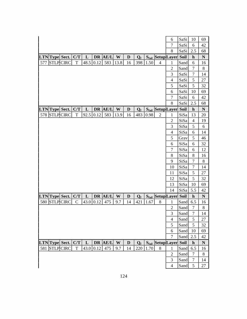
124

6 SaSi 10 69 7 SaSi 6 42 8 SaSi 2.5 68

LTN Type Sect. C/T L DR AE/L W D Qf Sfail Setup Layer Soil h N 577 STLP CIRC T 48.5 0.12 583 13.8 16 398 1.50 4 1 Sand 6 16

2 Sand 7 8 3 SaSi 7 14 4 SaSi 5 27 5 SaSi 5 32 6 SaSi 10 69 7 SaSi 6 42 8 SaSi 2.5 68

LTN Type Sect. C/T L DR AE/L W D Qf Sfail Setup Layer Soil h N 578 STLP CIRC T 92.5 0.12 583 13.9 16 483 0.98 2 1 SiSa 13 20

2 SiSa 4 19 3 SiSa 5 6 4 SiSa 6 14 5 Grav 5 46 6 SiSa 6 32 7 SiSa 6 12 8 SiSa 8 16 9 SiSa 7 8 10 SiSa 7 14 11 SiSa 5 27 12 SiSa 5 32 13 SiSa 10 69 14 SiSa 5.5 42

LTN Type Sect. C/T L DR AE/L W D Qf Sfail Setup Layer Soil h N 580 STLP CIRC C 43.0 0.12 475 9.7 14 421 1.67 8 1 Sand 6.5 16

2 Sand 7 8 3 Sand 7 14 4 Sand 5 27 5 Sand 5 32 6 Sand 10 69 7 Sand 2.5 42

LTN Type Sect. C/T L DR AE/L W D Qf Sfail Setup Layer Soil h N 581 STLP CIRC T 43.0 0.12 475 9.7 14 220 1.70 8 1 Sand 6.5 16

2 Sand 7 8 3 Sand 7 14 4 Sand 5 27

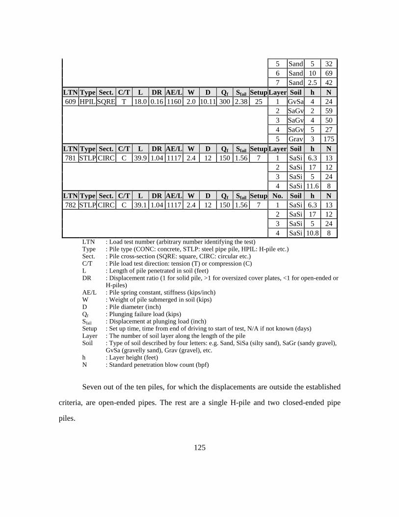
125

5 Sand 5 32 6 Sand 10 69 7 Sand 2.5 42

LTN Type Sect. C/T L DR AE/L W D Qf Sfail Setup Layer Soil h N 609 HPIL SQRE T 18.0 0.16 1160 2.0 10.11 300 2.38 25 1 GvSa 4 24

2 SaGv 2 59 3 SaGv 4 50 4 SaGv 5 27 5 Grav 3 175

LTN Type Sect. C/T L DR AE/L W D Qf Sfail Setup Layer Soil h N 781 STLP CIRC C 39.9 1.04 1117 2.4 12 150 1.56 7 1 SaSi 6.3 13

2 SaSi 17 12 3 SaSi 5 24 4 SaSi 11.6 8

LTN Type Sect. C/T L DR AE/L W D Qf Sfail Setup No. Soil h N 782 STLP CIRC C 39.1 1.04 1117 2.4 12 150 1.56 7 1 SaSi 6.3 13

2 SaSi 17 12 3 SaSi 5 24 4 SaSi 10.8 8

LTN : Load test number (arbitrary number identifying the test) Type : Pile type (CONC: concrete, STLP: steel pipe pile, HPIL: H-pile etc.) Sect. : Pile cross-section (SQRE: square, CIRC: circular etc.) C/T : Pile load test direction: tension (T) or compression (C) L : Length of pile penetrated in soil (feet) DR : Displacement ratio (1 for solid pile, >1 for oversized cover plates, <1 for open-ended or

H-piles) AE/L : Pile spring constant, stiffness (kips/inch) W : Weight of pile submerged in soil (kips) D : Pile diameter (inch) Qf : Plunging failure load (kips) Sfail : Displacement at plunging load (inch) Setup : Set up time, time from end of driving to start of test, N/A if not known (days) Layer : The number of soil layer along the length of the pile Soil : Type of soil described by four letters: e.g. Sand, SiSa (silty sand), SaGr (sandy gravel),

GvSa (gravelly sand), Grav (gravel), etc. h : Layer height (feet) N : Standard penetration blow count (bpf)

Seven out of the ten piles, for which the displacements are outside the established

criteria, are open-ended pipes. The rest are a single H-pile and two closed-ended pipe

piles.

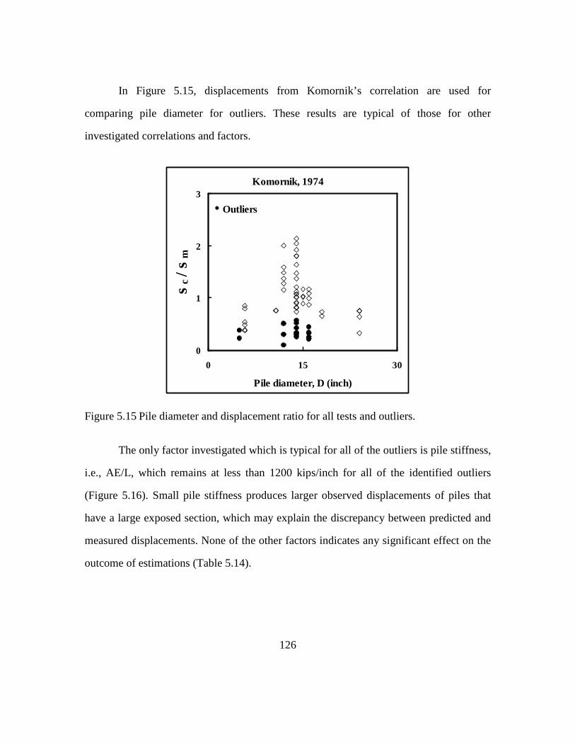
126

In Figure 5.15, displacements from Komornik’s correlation are used for

comparing pile diameter for outliers. These results are typical of those for other

investigated correlations and factors.

Komornik, 1974

0

1

2

3

0 15 30

Pile diameter, D (inch)

s c / s

m

• Outliers

Figure 5.15 Pile diameter and displacement ratio for all tests and outliers.

The only factor investigated which is typical for all of the outliers is pile stiffness,

i.e., AE/L, which remains at less than 1200 kips/inch for all of the identified outliers

(Figure 5.16). Small pile stiffness produces larger observed displacements of piles that

have a large exposed section, which may explain the discrepancy between predicted and

measured displacements. None of the other factors indicates any significant effect on the

outcome of estimations (Table 5.14).

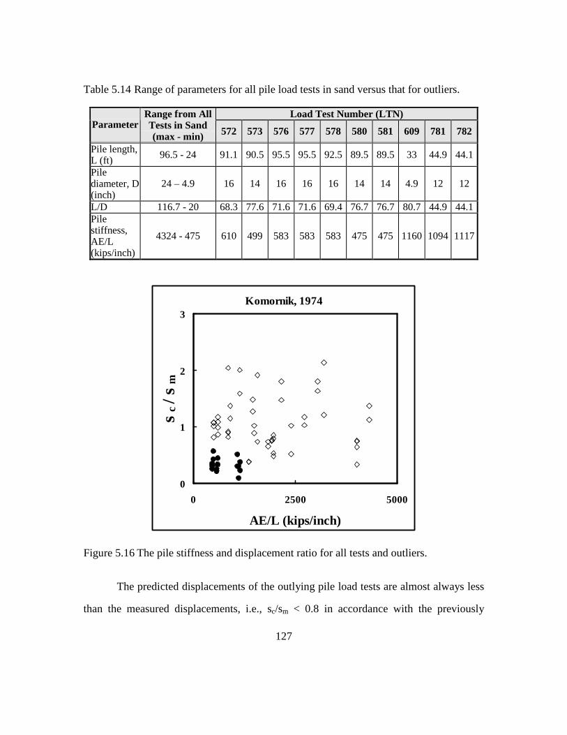
127

Table 5.14 Range of parameters for all pile load tests in sand versus that for outliers.

Load Test Number (LTN) Parameter

Range from All Tests in Sand (max - min) 572 573 576 577 578 580 581 609 781 782

Pile length, L (ft) 96.5 - 24 91.1 90.5 95.5 95.5 92.5 89.5 89.5 33 44.9 44.1

Pile diameter, D (inch)

24 – 4.9 16 14 16 16 16 14 14 4.9 12 12

L/D 116.7 - 20 68.3 77.6 71.6 71.6 69.4 76.7 76.7 80.7 44.9 44.1 Pile stiffness, AE/L (kips/inch)

4324 - 475 610 499 583 583 583 475 475 1160 1094 1117

Komornik, 1974

0

1

2

3

0 2500 5000

AE/L (kips/inch)

s c / s

m

Figure 5.16 The pile stiffness and displacement ratio for all tests and outliers.

The predicted displacements of the outlying pile load tests are almost always less

than the measured displacements, i.e., sc/sm < 0.8 in accordance with the previously

128

established criteria. A few predictions using Frank’s correlation and elastic column are

exceptions. Contrary to the tests in cohesive soils, the erroneous estimations may be

attributed to one or many of the following factors:

– All but three (LTN’s: 572, 573 and 578) of the piles are driven through a larger

casing or excavation through the top layers. At Site 2 of I5/I8 Indicator Pile Test Program

(LTN’s from 576 through 581), the casing depth reached 47 feet. Cased portions of a pile

are considered in the Tapile program by assuming that these sections are part of the

exposed length of the pile. Therefore, cased sections do not provide any load carrying

capacity and displace as a free-standing column. The elastic compression or tension of

the exposed pile column is then simply added to the movement of the lower sections of

the pile that are in contact with soil. However, the effect of the displacements from the

upper sections to the lower sections in is disregarded, which possibly may lead to lower

predicted displacements than those measured in pile load tests.

– No borings were conducted at or near the location of the pile load test (LTN:

572, 573 and 609). Consequently, soil profiles and SPT blow counts had to be estimated

from pile driving records, for which the accuracy is questionable.

5.4 M IXED PROFILES

FinalCT database contains 83 pile load tests that are driven into mixed profiles.

Displacements of piles driven into mixed soils are predicted using the correlations

denoted with (*) in Tables 5.1 and 5.8. Twelve predictions are made for each pile load

test at load ratios up to a half.

129


All of the measured displacements are less than |0.35| inches (Figure 5.17). The

magnitude of displacements is within a smaller range in mixed profiles than those in

clayey or sandy soils.

0

20

40-0

.3

-0.2

-0.1 0

0.1

0.2

0.3

0.4

D i s p l a c e m e n t ( i n c h )

N u

m b

e r

Third

Half

Figure 5.17 Magnitudes of measured displacements.

The sm/D for axial loads up to half of peak applied load is shown in Figure 5.18.

For a load ratio of a third, all but three of the tests had an upper limit of sm/D = 1%. The

upper limit reaches sm/D = 2% at a load ratio of a half.

130

0

20

40

0 0.5 1 1.5

s m / D ( % )

N u

m b

e r

Third

Half

Figure 5.18 Absolute value of measured displacements, sm, divided by pile diameter, D.

5.4.2 Measured versus Predicted Displacements

A typical example of the comparison between estimated and measured

displacements up to a load ratio of a half is given in Figure 5.19, where Komornik’s

correlation for cohesionless soils is combined with Aschenbrener’s and Poulos’

suggestions for cohesive soils. Displacements are approximately less than |0.30| inches

with little variability between correlations. The predicted displacements are less than the

measured values in most cases, especially when Aschenbrener’s equation for cohesive

soils is used with any of the correlations for cohesionless soils.

131

Aschenbrener/Komornik

0

0.4

-0.4 0 0.4s m ( i n c h )

s c

( i n

c h

)

ThirdHalfsc=sm

TENS. COMP.

Poulos/Komornik

0

0.4

-0.4 0 0.4s m ( i n c h )

s c

( i n

c h

)

ThirdHalfsc=sm

TENS. COMP.

Figure 5.19 Comparison of displacements for piles driven into mixed profiles (N = 83).

A comparison of the displacements indicates a larger dispersion as the applied

load is increased from a third to a half although the error remains small, reinforcing the

idea that the elastic method is applicable for load ratios up to a half.

Overall the values of calculated displacements are similar between predictions if

they are grouped according to the correlation employed for cohesive soil layers. For

example, all of the displacements calculated with Aschenbrener’s correlation for Young’s

132

modulus in cohesive layers result in almost the same spread and dispersion data

irrespective of the correlation employed for cohesionless layers.

Use of Frank’s method generally led to overprediction of displacements (Figure

5.20). The formulation is intended as an upper-limit value for displacements at a load

equal to half of the pile capacity. Although most of the estimations are too large to be

accurate, the method may provide a reasonable first guess of expected displacements at

low load ratios. Predictions based on the elastic column vary within a narrow band

although they tend to be larger than measurements in most cases (Figure 5.21). The

elastic column provides a simple and quick approach to predict displacements simply and

quickly.

Frank

0

0.5

-0.5 0 0.5s m ( i n c h )

s c

( i n

c h

)

ThirdHalfsc=sm

TENS. COMP.

Figure 5.20 Comparison of displacements predicted using Frank’s correlation.

133

Elastic column

0

0.4

-0.4 0 0.4s m ( i n c h )

s c

( i n

c h

)

ThirdHalfsc=sm

TENS. COMP.

Figure 5.21 Predictions utilizing the elastic column approach in mixed profiles.


The predicted displacements are in-large-part less than those measured in pile

load tests. The majority (varying from 68% to 85%) of the displacement ratios obtained

by pairing Aschenbrener’s correlation with those recommended for cohesionless soils are

between 0.2 and 1, thus further attesting to the underestimation of actual displacements.

In contrast, the same range of displacement ratios obtained by combining the same

correlations with Poulos varies from 41% to 64%. The scatter is over wider displacement

ratios utilizing Poulos’ correlation for cohesive soil layers than the spread for the same

correlations with Aschenbrener, whereas the scatter was similar for predictions for

cohesive soils only.

Frank’s correlation leads to larger predicted displacements than those measured in

pile load tests for about 85% of the comparisons with 68% of the predictions resulting in

displacement ratios in excess of 1.6. Large displacement ratios, up to 24.7, indicate the

low reliability of this correlation.

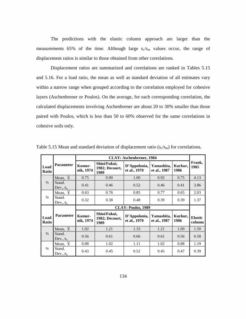
134

The predictions with the elastic column approach are larger than the

measurements 65% of the time. Although large sc/sm values occur, the range of

displacement ratios is similar to those obtained from other correlations.

Displacement ratios are summarized and correlations are ranked in Tables 5.15

and 5.16. For a load ratio, the mean as well as standard deviation of all estimates vary

within a narrow range when grouped according to the correlation employed for cohesive

layers (Aschenbrener or Poulos). On the average, for each corresponding correlation, the

calculated displacements involving Aschenbrener are about 20 to 30% smaller than those

paired with Poulos, which is less than 50 to 60% observed for the same correlations in

cohesive soils only.

Table 5.15 Mean and standard deviation of displacement ratio (sc/sm) for correlations.

CLAY: Aschenbrener, 1984

Load Ratio

Parameter Komor-nik, 1974

Shioi/Fukui, 1982; Decourt, 1989

D’Appolonia, et al., 1970

Yamashita, et al., 1987

Kurkur, 1986

Frank, 1985

Mean, x 0.75 0.90 1.00 0.92 0.75 4.13 ⅓ Stand.

Dev., sx 0.41 0.46 0.52 0.46 0.41 3.86

Mean, x 0.63 0.76 0.85 0.77 0.65 2.03 ½ Stand.

Dev., sx 0.32 0.38 0.48 0.39 0.39 1.37

CLAY: Poulos, 1989

Load Ratio





Kurkur, 1986

Elastic column

Mean, x 1.02 1.21 1.33 1.21 1.00 1.50 ⅓ Stand.

Dev., sx 0.56 0.61 0.66 0.61 0.56 0.58

Mean, x 0.88 1.02 1.11 1.02 0.88 1.19 ½ Stand.

Dev., sx 0.43 0.45 0.52 0.45 0.47 0.39

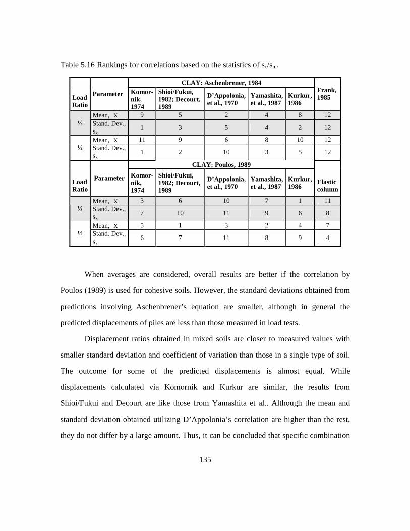
135

Table 5.16 Rankings for correlations based on the statistics of sc/sm.


Load Ratio





Kurkur, 1986

Frank, 1985

Mean, x 9 5 2 4 8 12 ⅓ Stand. Dev.,

sx 1 3 5 4 2 12

Mean, x 11 9 6 8 10 12 ½ Stand. Dev.,

sx 1 2 10 3 5 12

CLAY: Poulos, 1989

Load Ratio





Kurkur, 1986

Elastic column

Mean, x 3 6 10 7 1 11 ⅓ Stand. Dev.,

sx 7 10 11 9 6 8

Mean, x 5 1 3 2 4 7 ½ Stand. Dev.,

sx 6 7 11 8 9 4

When averages are considered, overall results are better if the correlation by

Poulos (1989) is used for cohesive soils. However, the standard deviations obtained from

predictions involving Aschenbrener’s equation are smaller, although in general the

predicted displacements of piles are less than those measured in load tests.

Displacement ratios obtained in mixed soils are closer to measured values with

smaller standard deviation and coefficient of variation than those in a single type of soil.

The outcome for some of the predicted displacements is almost equal. While

displacements calculated via Komornik and Kurkur are similar, the results from

Shioi/Fukui and Decourt are like those from Yamashita et al.. Although the mean and

standard deviation obtained utilizing D’Appolonia’s correlation are higher than the rest,

they do not differ by a large amount. Thus, it can be concluded that specific combination

136

of correlations for Young’s modulus does not have a significant impact on the estimated

displacements in mixed profiles when load ratios are equal to or less than a half. Within

the context of this dissertation, any combination of the correlations for cohesive soils

with those for cohesionless soil will result in similar outcomes. The use of elastic method

is likely the main reason for such a conclusion.


All of the displacement differences obtained from predictive methods, with the

exception of those from Frank, result in similar outcomes regardless of the correlation

used for cohesive and cohesionless layers. Over 90% of the displacement differences are

less than 0.1 inch of the measured values. The range of displacement differences,

corresponding average and standard deviation values for each load ratio are positive and

almost the same (Table 5.17).

Table 5.17 Summary of the mean and standard deviation for displacement differences (all in inches).


Load Ratio


Shioi/ Fukui, 1982; Decourt, 1989



Kurkur, 1986

Frank, 1985

Mean,x 0.00 0.00 0.01 0.00 0.00 -0.04 ⅓

Stand. Dev., sx 0.04 0.04 0.04 0.04 0.04 0.19 Mean,x 0.01 0.02 0.03 0.02 0.02 -0.04

½ Stand. Dev., sx 0.08 0.07 0.08 0.07 0.08 0.15

CLAY: Poulos, 1989

Load Ratio





Kurkur, 1986

Elastic column

Mean,x 0.00 0.01 0.01 0.01 0.00 0.01 ⅓

Stand. Dev., sx 0.04 0.04 0.04 0.04 0.04 0.05 Mean,x 0.01 0.02 0.03 0.02 0.02 0.02

½ Stand. Dev., sx 0.07 0.06 0.07 0.06 0.07 0.06

137

5.4.5 Outliers

Out of 83 pile load tests, there is only one (1.2%) for which all but one (LTN:

789) of the predictive methods results in overestimation of measured displacements. The

load-displacement curve for this particular test is almost linear without any break to

indicate the capacity because the pile load testing had to be terminated prematurely due to

equipment failure. Therefore, the measured loads as well as displacements are

significantly less than what would be observed if the testing had been successful. Another

factor that could lead to larger displacements is the small shear strength values from

laboratory tests. Interestingly, for this pile load test, the only prediction that is close to the

measurements is obtained by the elastic column approach. The outcome may provide an

example for the effect of a load test that was terminated before reaching failure.

5.5 CONCLUSIONS

In this study, correlations from the literature are used for load ratios up to a half to

predict displacements, which are compared with the measurements from pile load tests.

5.5.1 Piles in Cohesive Soils (N = 26)

All of the measured displacements are less than an absolute value of 0.25 inches

up to a load ratio of a half, where a displacement to pile diameter ratio, ρ/D, of 1.5% is

determined to be a reasonable first estimate. A direct comparison of predicted and

measured displacements provides good overall agreement, although their scatter increases

with increasing load ratio. For all of the predictive methods, the loading direction does

not appear to affect the outcome. The mean and standard deviation of the displacement

ratio (sc/sm) and displacement difference (sc-sm) for each load ratio are presented in

Tables 5.18 and 5.19.

138

Table 5.18 The statistics for the displacement ratios (sc/sm) in cohesive soils.


(1989)

Poulos (1972)

(driven)



Callanan/ Kulhawy 1985; Johnson 1986

Frank 1985

Elastic column

Mean, x 1.76 1.81 3.09 1.15 2.44 3.25 1.63 ⅓


Table 5.19 Mean and standard deviation of displacement differences (sc-sm).

Load Ratio Value (inch) Poulos,

(1989)

Poulos, (1972)

(driven)

Poulos, (1972) (bored)

Aschenbre-ner, (1984)

Callanan/ Kulhawy

1985; Johnson 1986

Frank, 1985

Elastic column

Mean, x -0.01 -0.01 -0.01 -0.02 -0.01 0.00 0.00 ⅓


The correlations can be ranked starting from the best as: elastic column,

Aschenbrener (1984), Poulos (1989), and Poulos (1972, driven piles). These findings

coincide with the conclusions reached visually from a direct comparison of the

displacements.

The mean values of displacement differences for each prediction are not large and

the standard deviation does not change significantly with increased loading.

Three out of seven predictive methods utilized result in predictions that have a

large mean and standard deviation for sc/sm: Callanan and Kulhawy (1985)/Johnson

(1986), Poulos (1972, bored pile), and Frank (1985).

Four pile load tests are consistently identified as outliers for all the predictions.

However, none of the investigated parameters explain this outcome.

139

5.5.2 Piles in Cohesionless Soils (N = 34)

For load ratios up to a half, the absolute values of all of the measured

displacements are less than 0.5 inches and have ρ/D=2.5%. The pile loading direction

does not affect the predicted displacements. Displacements estimated at the load ratio of a

third conform better to the measured displacements than those at a half. The calculated

displacement ratios and differences are summarized in Tables 5.20 and 5.21.

Table 5.20 Mean and standard deviation of the displacement ratio for predictive methods in cohesionless soils.

Load RatioValue

Komor-nik, 1974

Shioi/ Fukui, 1982;

Decourt, 1989

Den-ver, 1982

D’Appo-lonia et

al., 1970 (NC)

D’Appo-lonia et

al., 1970 (OC)

Chris-toulas, 1988

Yamas-hita et

al., 1987

Kur-kur, 1986

Frank, 1985

Elastic column

Mean,x 0.97 1.26 1.86 1.62 1.19 18.19 1.16 0.79 2.74 1.24 ⅓ St.

Dev., sx 0.58 0.80 1.23 1.16 0.75 91.96 0.71 0.48 2.88 0.62

Mean,x 0.74 0.96 1.43 1.26 0.90 16.92 0.88 0.62 0.94 0.93 ½ St.

Dev., sx 0.42 0.61 0.91 0.75 0.50 87.24 0.49 0.35 1.19 0.42

Table 5.21 The statistics of displacement difference (sc-sm) for predictive methods in cohesionless soils.

Load Ratio

Value (inch)

Komor-nik, 1974

Shioi/ Fukui, 1982;

Decourt, 1989

Den-ver, 1982

D’Appo-lonia et

al., 1970 (NC)

D’Appo-lonia et

al., 1970 (OC)

Yamas-hita et

al., 1987

Kur-kur, 1986

Frank, 1985

Elastic column

Mean,x 0.00 0.01 0.02 0.02 0.01 0.01 0.00 -0.02 -0.01 ⅓ St.

Dev., sx 0.06 0.06 0.07 0.07 0.06 0.06 0.07 0.09 0.06

Mean,x 0.01 0.02 0.05 0.04 0.02 0.02 0.01 -0.02 -0.01 ½ St.

Dev., sx 0.14 0.13 0.15 0.13 0.13 0.13 0.14 0.11 0.10

140

Predictions using Young’s modulus as suggested by Komornik are the best at a

load ratio of a third, despite having a slightly increased standard deviation. The elastic

column approach is the best overall estimator at or near a load ratio of a half.

The correlations by Denver (1982), D’Appolonia et al. (1970a, normally

consolidated), Christoulas (1988), and Frank (1985) result in estimates for displacement

that can vary significantly from those measured in pile load tests.

For ten out of 34 pile load tests, the predicted displacements are much lower than

the measured displacements. The only investigated factor, which may explain the

underestimation of displacements for pile load tests is pile stiffness, i.e., AE/L, which

remains at less than 1200 kips/inch for all the identified outliers.

5.5.3 Piles in Mixed Profiles (N = 83)

Up to a load ratio of a half, all of the measured displacements are less than a half

inch, of which 92% are less than a quarter inch. All of the measured displacements are

scattered within 1% and 1.5% of the pile diameter at a load ratio of a third and a half,

respectively. Tension or compression loading does not have a significant impact on the

predicted displacements. On the average, correlations for cohesionless material that are

paired with Poulos’ equation for cohesive soils produce 20% to 30% lower displacements

than those paired with Aschenbrener, although the standard deviation also increases. The

results of comparing predictions and measurements are summarized in Tables 5.22 and

5.23.

Within the bounds of the predictive methods investigated in this study, any

combinations of two correlations, –one for cohesive and another for cohesionless layers,

result in similar outcomes.

141

Table 5.22 Statistics of displacement ratio (sc/sm) for predictions in mixed profiles.

CLAY: Aschenbrener, 1984 Lo

ad R

atio

Komornik, 1974




Kurkur, 1986

Frank, 1985

Mean 0.75 0.90 1.00 0.92 0.75 4.13 ⅓

Stand. Dev. 0.41 0.46 0.52 0.46 0.41 3.86 Mean 0.63 0.76 0.85 0.77 0.65 2.03

½ Stand. Dev 0.32 0.38 0.48 0.39 0.39 1.37

CLAY: Poulos, 1989

Load

Rat

io

Komornik, 1974




Kurkur, 1986

Elastic column

Mean 1.02 1.21 1.33 1.21 1.00 1.50 ⅓

Stand. Dev. 0.56 0.61 0.66 0.61 0.56 0.58 Mean 0.88 1.02 1.11 1.02 0.88 1.19

½ Stand. Dev. 0.43 0.45 0.52 0.45 0.47 0.39

Table 5.23 Summary of mean and standard deviation for displacement differences of predictions with measurements.


Load

Rat

io

(all in inches)

Komor-nik, 1974




Kurkur, 1986

Frank, 1985

Mean,x 0.00 0.00 0.01 0.00 0.00 -0.04 ⅓

Stand. Dev., sx 0.04 0.04 0.04 0.04 0.04 0.19 Mean,x 0.01 0.02 0.03 0.02 0.02 -0.04

½ Stand. Dev., sx 0.08 0.07 0.08 0.07 0.08 0.15

CLAY: Poulos, 1989

Load

Rat

io

(all in inches)

Komor-nik, 1974




Kurkur, 1986

Elastic column

Mean,x 0.00 0.01 0.01 0.01 0.00 0.01 ⅓

Stand. Dev., sx 0.04 0.04 0.04 0.04 0.04 0.05 Mean,x 0.01 0.02 0.03 0.02 0.02 0.02

½ Stand. Dev., sx 0.07 0.06 0.07 0.06 0.07 0.06

5.6 SUMMARY

In this chapter, direct predictive methods of displacements along with routinely

employed correlations for soil Young’s modulus are introduced and utilized in

142

conjunction with the elastic method for predicting displacements within half of the peak

applied loads or “working loads” for which the correlations are proposed.

These correlations (five for cohesive soils, ten for piles in cohesionless and mixed

profiles) involve triaxial undrained shear strength, cu, and standard penetration blow

count, N, for cohesive and cohesionless soil layers, respectively.

Separate comparisons are made for cohesive, cohesionless and mixed profiles.

The relative magnitudes of estimated and measured displacements up to a load ratio of a

half are established in terms of their absolute values as well as their percentage of the pile

diameter. Estimated displacements are then compared graphically and statistically with

those measured from pile load tests included in the Caltrans database. Results that vary

significantly from others in terms of displacement ratio (sc/sm) and displacement

difference (sc-sm) are identified. Various factors affecting these results are further

examined in an attempt to determine their respective influences. The selected correlations

are then ranked based on the outcome of these analyses.

143

Chapter 6: Proposed Method of Predicting Displacements

6.1 INTRODUCTION

Young’s modulus of soil decreases with increasing applied loads on a pile

comparable to a secant modulus from a stress-strain curve. Young’s modulus values

calculated at varying loads may then be used to construct the load-displacement curve for

an axially loaded pile.

A new predictive method based on data from pile load tests provided by Caltrans

is proposed to calculate displacements at various applied loads. The aim is to develop a

more accurate and reliable method for determining the displacement of axially loaded

piles in compression as well as in tension. The proposed correlations are developed using

data from piles in cohesive soils and separately for piles in cohesionless soils and are then

applied to piles in mixed profiles as independent measures of validity.

The analytical approach to determine Young’s moduli used in the following

sections are outlined in Chapter 4.

6.2 COHESIVE SOILS

The changes of Young’s modulus, Es, with undrained shear strength are presented

in Figure 6.1 separately for each load test direction and load ratio (⅓, ½, and ⅔). Some

trends can be observed:

- Young’s modulus increases with increasing cu. The scatter of points from the

mean is substantial.

- Tension and compression tests seem to yield the same values of Es at any cu.

144

0

1000

2000

3000

0 1 2 3

Undrained Shear Strength, cu (ksf)

Es

(ksf)

a)

Comp (⅓)Tens (⅓)

0

1000

2000

3000

0 1 2 3


Es

(ksf)

b)

Comp (½)Tens (½)

0

1000

2000

3000

0 1 2 3


Es

(ksf)

c)

Comp (⅔)Tens (⅔)

Figure 6.1 Young’s modulus versus undrained shear strength for each load ratio (N=26).

Low values of undrained shear strength can be seen better when the Es-cu relation

is depicted on a logarithmic scale (Figure 6.2a and b). The outcome for load ratios of a

third and a half are similar and are shown together. The suggested linear correlation for

the Es-cu relationship is also given, which was obtained by minimizing the differences in

the suggested and calculated Young’s moduli. The correlation factor between Es and cu is

given to only one significant figure to reflect the substantial scatter.

145

Young’s modulus decreases as the load ratios increase because of the curvature of

the load-displacement curves.

10

100

1000

10000

0.1 1 10


Es

(ksf)

Es = 400cu

a)

Comp (½) Tens (½)Comp (⅓) Tens (⅓)

10

100

1000

10000

0.1 1 10


Es

(ksf)

Es=300cu

b)


Figure 6.2 Change of Young’s modulus with undrained shear strength and fitted correlations.

Overall, the calculated displacements compare well with the measured

displacements in pile load tests (Figure 6.3 and Table 6.1). However, the mean values of

sc/sm are higher than one for all load ratios although sc-sm values remain small. Larger

ratios can be expected when such small displacements are involved.

146

0

0.6

-0.6 0 0.6

Meas. displacement, sm (inch)

Ca

lc. d

ispl

ace

men

t, s c

(inch

)

Akgüner 07Series2sc=sm

Figure 6.3 Calculated and measured displacements using suggested correlations.

Table 6.1 Summary statistics for (sc/sm) and (sc-sm) employing the proposed method (N=26).

Statistics for (sc/sm) Third Half Two-Third Mean, x 1.49 1.21 1.19 Standard Dev., sx 1.09 0.62 0.53 cov (%) 72.9 51.6 45.0 Maximum 5.92 3.17 2.68 Minimum 0.44 0.36 0.38 Statistics for (sc-sm) Third Half Two-Third Mean, x (inch) -0.01 -0.01 0.00 Standard Dev., sx (inch) 0.05 0.07 0.10 Maximum 0.07 0.14 0.19 Minimum -0.11 -0.21 -0.31

The averages for sc/sm are higher than one because the Es-cu correlation was

developed to minimize the difference between the suggested and observed Es. For small

displacements as measured for load ratios less than approximately half to two-thirds,

small variations in displacements affect the outcome of sc/sm significantly. Therefore, the

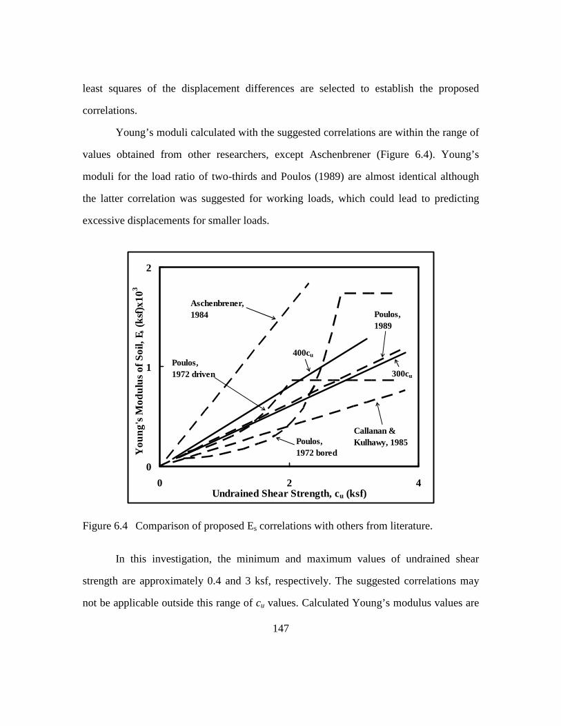
147

least squares of the displacement differences are selected to establish the proposed

correlations.

Young’s moduli calculated with the suggested correlations are within the range of

values obtained from other researchers, except Aschenbrener (Figure 6.4). Young’s

moduli for the load ratio of two-thirds and Poulos (1989) are almost identical although

the latter correlation was suggested for working loads, which could lead to predicting

excessive displacements for smaller loads.

0

1

2

0 2 4Undrained Shear Strength, cu (ksf)

Yo

un

g's

Mo

du

lus

of S

oil,

E s (

ksf)

x103

Aschenbrener,1984 Poulos,

1989

Poulos,1972 driven

Poulos,1972 bored

Callanan &Kulhawy, 1985

300cu

400cu

Figure 6.4 Comparison of proposed Es correlations with others from literature.

In this investigation, the minimum and maximum values of undrained shear

strength are approximately 0.4 and 3 ksf, respectively. The suggested correlations may

not be applicable outside this range of cu values. Calculated Young’s modulus values are

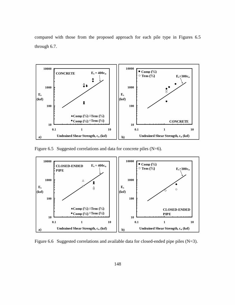
148

compared with those from the proposed approach for each pile type in Figures 6.5

through 6.7.

10

100

1000

10000

0.1 1 10


Es

(ksf)

Es = 400cu

a)


CONCRETE

10

100

1000

10000

0.1 1 10


Es

(ksf)

Es=300cu

b)


CONCRETE

Figure 6.5 Suggested correlations and data for concrete piles (N=6).

10

100

1000

10000

0.1 1 10


Es

(ksf)

Es = 400cu

a)


CLOSED-ENDEDPIPE

10

100

1000

10000

0.1 1 10


Es

(ksf)

Es=300cu

b)


CLOSED-ENDEDPIPE

Figure 6.6 Suggested correlations and available data for closed-ended pipe piles (N=3).

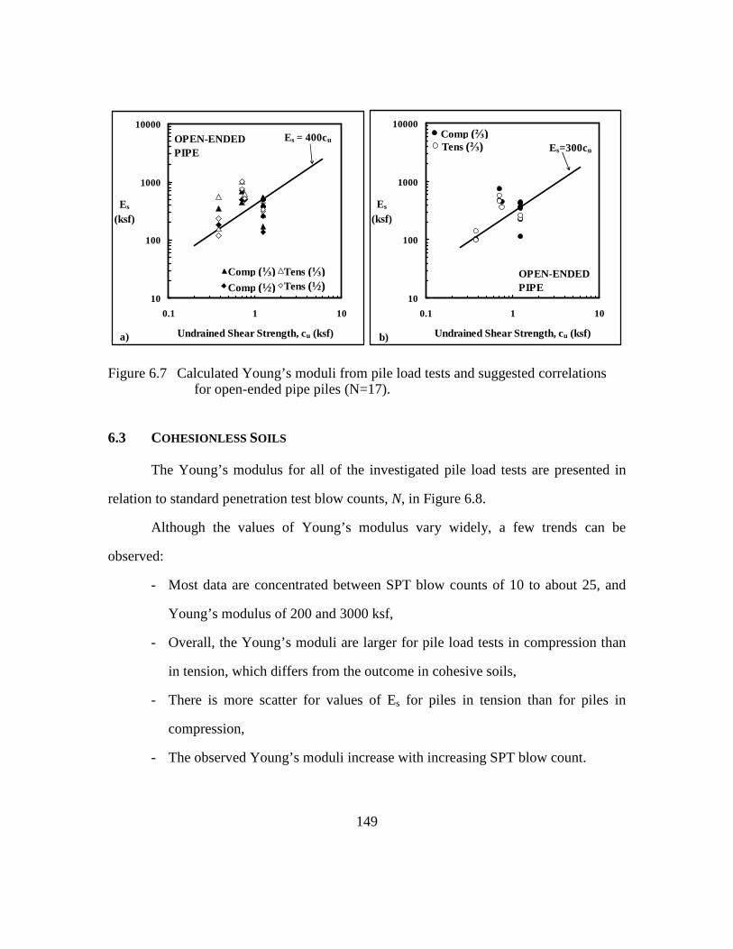
149

10

100

1000

10000

0.1 1 10


Es

(ksf)

Es = 400cu

a)


OPEN-ENDEDPIPE

10

100

1000

10000

0.1 1 10


Es

(ksf)

Es=300cu

b)


OPEN-ENDEDPIPE

Figure 6.7 Calculated Young’s moduli from pile load tests and suggested correlations for open-ended pipe piles (N=17).

6.3 COHESIONLESS SOILS

The Young’s modulus for all of the investigated pile load tests are presented in

relation to standard penetration test blow counts, N, in Figure 6.8.

Although the values of Young’s modulus vary widely, a few trends can be

observed:

- Most data are concentrated between SPT blow counts of 10 to about 25, and

Young’s modulus of 200 and 3000 ksf,

- Overall, the Young’s moduli are larger for pile load tests in compression than

in tension, which differs from the outcome in cohesive soils,

- There is more scatter for values of Es for piles in tension than for piles in

compression,

- The observed Young’s moduli increase with increasing SPT blow count.

150

0

8

16

0 50 100

SPT N (bpf)

Es

x1000(ksf)

Comp (⅓) Tens (⅓)

a)

0

3

6

0 50 100SPT N (bpf)

Es

x1000(ksf)

Comp (½) Tens (½)

b)

0

3

6

0 50 100

SPT N (bpf)

Es

x1000(ksf)

Comp (⅔) Tens (⅔)

c)

Figure 6.8 Variations of Young’s modulus with SPT blow count (N=34).

A reasonable linear relationship between Young’s modulus and SPT blow counts

cannot be established. Therefore, a logarithmic fit to the calculated Young’s moduli for

each load ratio has been adopted in order to provide an approximation (Figure 6.9), which

minimizes the difference between the suggested Young’s moduli and those obtained from

pile load tests. The values of Young’s moduli are depicted against log(N) to develop an

equation of the form (also shown in Figure 6.9):

151

s eE =a+b log (N)× ..................................................................................(6.1),

The range of SPT blow counts used for the suggested correlations varies from

eleven to 83.

Es(comp)=1.4Ln(N)-2.2

Es(tens)=0.9Ln(N)-2.0

0

3

6

10 100SPT N (bpf)

Es

x103

(ksf)

Comp (⅓) Tens (⅓)

a)

Es(comp)=1.8Ln(N)-3.8

Es(tens)=

0.4Ln(N)-0.7

0

3

6

10 100SPT N (bpf)

Es

x103

(ksf)

Comp (½) Tens (½)

b)

Es (comp) = 2.0Ln(N)-4.4

Es (tens) =

0.3Ln(N)-0.5

0

3

6

10 100SPT N (bpf)

Es

x103

(ksf)

Comp (⅔) Tens (⅔)

c)

Figure 6.9 Young’s modulus versus blow count in logarithmic axes given along with fitted curves (N=31).

152

Three of the load tests (LTNs: 495, 571 and 752) were excluded in developing the

fitted curves. Load testing for one of the piles (14-inch concrete, LTN: 495) was

terminated early at a displacement of 0.5 inch before an actual failure load could be

reached. Therefore, the measured displacements are smaller and in turn the calculated

Young’s modulus larger than the rest of the load tests. The second pile (16x0.5 inch

open-ended pipe, LTN: 571) had about 40 feet from the tip of the pile which was

plugged, which is significant for a pile that has penetrated 43 feet into the ground and

also unusual for non-displacement piles. The site characterization for the third excluded

pile (12-inch concrete, LTN: 752) was based on a boring that was over 100 feet away;

therefore, the soil layering and properties may not correspond to the conditions at the

location of the pile.

With respect to the three rejected tests, the question arose as to whether it was

likely that incorrect N values or errors in measuring settlements could be the cause of the

variation between measured and computed settlements. Analyses demonstrated that

unreasonably high values of N were required to bring data from the three rejected tests

into the scatter band of the other tests so that explanation of their outlier status seems

unlikely. Alternatively, small errors in the measured settlement could cause large errors

in sc/sm. The measured displacements at the on-set of a pile load test are typically small

and prone to equipment or personnel errors. The values of Young’s modulus for the

excluded tests are considerably higher than the rest of the results. The measured

displacements are increased between 0.005 and 0.01 inches to decrease the observed

values of Young’s modulus (Figure 6.10). Such small variations have an important

impact on the outcome.

153

All of the correlations for all load ratios are shown together in Figure 6.11. The

correlations for piles tested in compression have approximately the same increasing trend

for the Young’s modulus, which for all practical purposes can be replaced by a single

relationship applicable to all load ratios.

Fitted curves are compared with other correlations recommended in the literature

(Figure 6.12).

Predicted displacements are larger than the measured displacements (Figure 6.13)

although the differences remain small. The statistical values of the displacement ratio and

displacement differences are provided in Table 6.2.

0

5

10

15

10 100SPT N (bpf)

Es

x103

(ksf)

sm

sm+0.005"

sm+0.01"

Figure 6.10 The effect of varying displacements on the values of Young’s modulus.

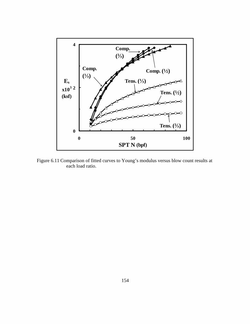
154

0

2

4

0 50 100

SPT N (bpf)

Es

x103

(ksf)

Tens. (⅓)

Tens. (½)

Tens. (⅔)

Comp.

(⅓)

Comp.

(⅔)

Comp. (½)

Figure 6.11 Comparison of fitted curves to Young’s modulus versus blow count results at each load ratio.

155

0

2

4

0 25 50SPT N60 (bpf)

Es

(ksf)

x103

Comp.

Komornik, 1974

Yamashita1987

Tens. (⅔)

(½)

Shioi&Fukui1982

D'Appolonia et al.,1970, OC

(⅓)

Figure 6.12 Fitted curves in relation to other recommended correlations for cohesionless soils.

Table 6.2 Statistical values for displacement ratios and differences in cohesionless soils (N=34).

Statistics (sc/sm) Third Half Two-Thirds Mean, x 1.16 1.10 1.24 Standard Dev., sx 0.68 0.54 0.63 cov (%) 58.1 48.9 51.0 Statistics (sc-sm) Third Half Two-Thirds Mean, x (inch) 0.01 0.00 0.00 Standard Dev., sx (inch) 0.06 0.13 0.19

Calculated Young’s moduli are given in Figures 6.14 through 6.18 for all load

ratios and loading directions, although no correlations have been deduced based on pile

156

type. Most of the Young’s moduli for concrete piles are higher than those suggested by

the fitted curves. Four of the six concrete piles are from the same location and have a

high stiffness ranging from 2200 to 4300 kips/inch.

0

0.5

1

-1 -0.5 0 0.5 1

sm (inch)

sc

(inch)

COMP.TENS. Akgüner 07sc = sm

Figure 6.13 Displacements calculated for piles in cohesionless soils using correlations derived from Caltrans database.

157

0

3

6

10 100SPT N (bpf)

Es

x103

(ksf)

Comp.(⅓)

(⅔)(½)Tension

CLOSED-ENDED

Comp (⅔)Comp (⅓) Comp (½)

Figure 6.14 Values of Young’s modulus obtained for the closed-ended pipe pile (N=1).

0

3

6

10 100SPT N (bpf)

Es

x103

(ksf)

Comp.(⅓)

(⅔)(½)Tension

CONCRETE-FILLED OPEN-ENDED

Comp (⅔)Comp (⅓) Comp (½)

Figure 6.15 Calculated Young’s modulus for concrete-filled pipe piles (N=2).

158

0

3

6

10 100SPT N (bpf)

Es

x103

(ksf)

Comp.(⅓)

(⅔)(½)Tension

Comp (⅔)Comp (⅓) Tens (⅓)

Tens (⅔)Tens (½)Comp (½)

H-PILE

Figure 6.16 Young’s modulus values calculated from H-piles in Caltrans pile load tests (N=4).

0

3

6

10 100SPT N (bpf)

Es

x103

(ksf)

Comp.(⅓)

(⅔)(½)Tension



CONCRETE

Figure 6.17 Variation of Es and N for concrete piles (N=6).

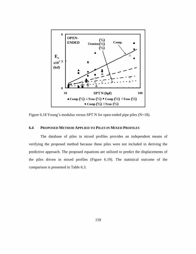
159

0

3

6

10 100SPT N (bpf)

Es

x103

(ksf)

Comp.(⅓)

(⅔)(½)Tension



OPEN-ENDED

Figure 6.18 Young’s modulus versus SPT N for open-ended pipe piles (N=18).

6.4 PROPOSED METHOD APPLIED TO PILES IN M IXED PROFILES

The database of piles in mixed profiles provides an independent means of

verifying the proposed method because these piles were not included in deriving the

predictive approach. The proposed equations are utilized to predict the displacements of

the piles driven in mixed profiles (Figure 6.19). The statistical outcome of the

comparison is presented in Table 6.3.

160

Suggested correlation

0

0.3

-0.3 0 0.3sm (inch)

sc(inch)

Thirdsc = sm

TENS. COMP.


0

0.5

-0.5 0 0.5sm (inch)

sc(inch)

Halfsc = sm

COMP.TENS.


0

0.6

-0.6 0 0.6sm (inch)

sc(inch)

Two-thirdsSeries2sc = sm

TENS. COMP.

Figure 6.19 Predicted and measured displacements of piles in mixed profiles (N=83).

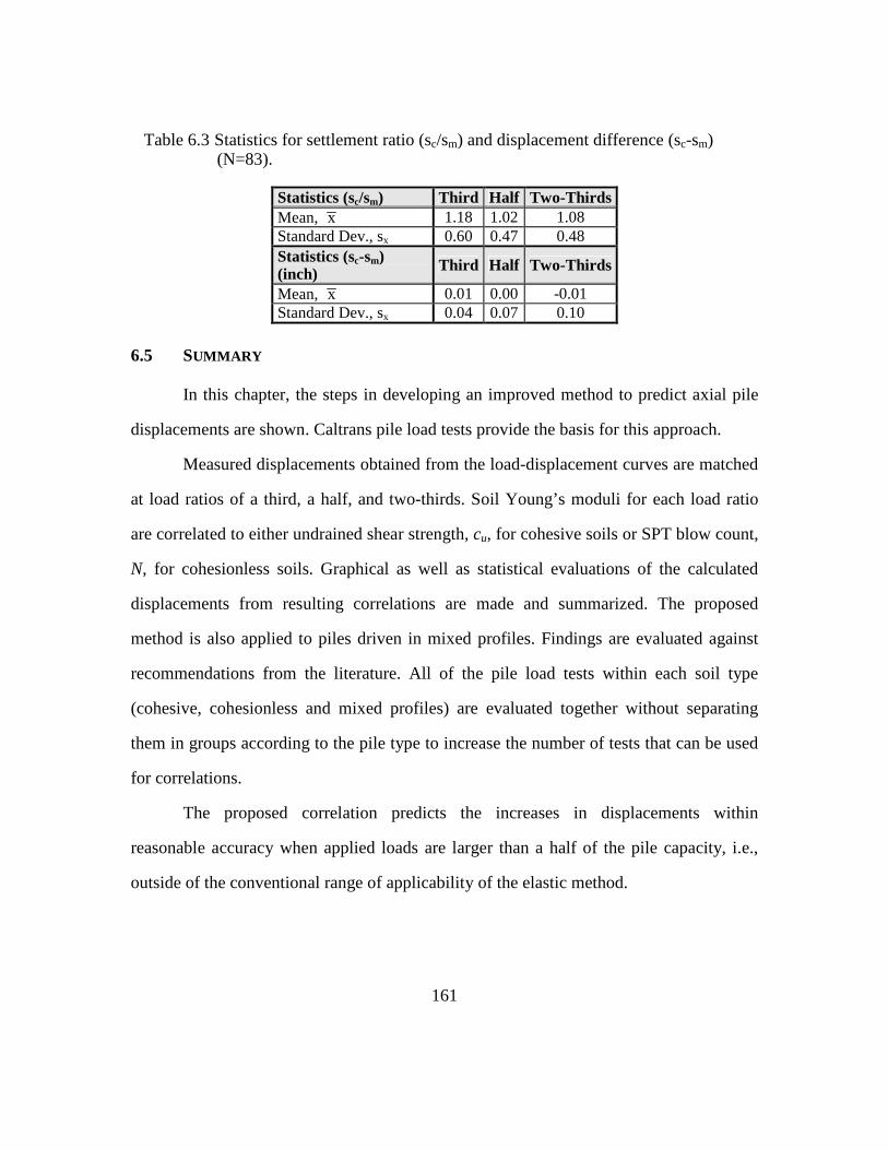
161

Table 6.3 Statistics for settlement ratio (sc/sm) and displacement difference (sc-sm) (N=83).

Statistics (sc/sm) Third Half Two-Thirds Mean, x 1.18 1.02 1.08 Standard Dev., sx 0.60 0.47 0.48 Statistics (sc-sm) (inch) Third Half Two-Thirds

Mean, x 0.01 0.00 -0.01 Standard Dev., sx 0.04 0.07 0.10

6.5 SUMMARY

In this chapter, the steps in developing an improved method to predict axial pile

displacements are shown. Caltrans pile load tests provide the basis for this approach.

Measured displacements obtained from the load-displacement curves are matched

at load ratios of a third, a half, and two-thirds. Soil Young’s moduli for each load ratio

are correlated to either undrained shear strength, cu, for cohesive soils or SPT blow count,

N, for cohesionless soils. Graphical as well as statistical evaluations of the calculated

displacements from resulting correlations are made and summarized. The proposed

method is also applied to piles driven in mixed profiles. Findings are evaluated against

recommendations from the literature. All of the pile load tests within each soil type

(cohesive, cohesionless and mixed profiles) are evaluated together without separating

them in groups according to the pile type to increase the number of tests that can be used

for correlations.

The proposed correlation predicts the increases in displacements within

reasonable accuracy when applied loads are larger than a half of the pile capacity, i.e.,

outside of the conventional range of applicability of the elastic method.

162

Chapter 7: Conclusions

The elastic method presents one of the most commonly used algorithms to

estimate displacements of foundations. It is based on Mindlin’s solution (1936) for

stresses and displacements due to a single vertical point load within a homogeneous,

isotropic half space. The objective of this dissertation research is to develop an improved

approach to predict the displacements of axially loaded single piles using the elastic

method. Poisson’s ratio, which has little effect on outcome, and Young’s modulus are the

two unknown parameters in this approach. An attempt is made to develop a

straightforward Young’s modulus correlation based on routinely available or obtained

parameters relying on a database containing pile load tests supplied by California

Department of Transportation (Caltrans), i.e., the FinalCT database. Separate analyses are

conducted on subsets of this database for each soil type, all of which are dominated by

open-ended pipe piles:

- twenty-six load tests on piles driven in primarily cohesive soils,

- thirty-four pile load tests founded in cohesionless soils,

- eighty-three tests in mixed profiles.

Within the context of this dissertation, almost all of the pile displacements that are

investigated are less than 0.5 inch exhibiting approximately a linear increase up to a load

of about two-thirds of the failure load. Non-linear behavior is observed when the loading

on the pile is in excess of 67% of the pile capacity. Therefore, it may be justified to

employ the elastic method for load ratios only up to a half, similar to the findings and

recommendations by other researchers.

In this research, the focus is on predicting immediate or short-term displacements

of driven piles. The first step in predicting pile displacements is to determine the pile

163

capacity, which in this dissertation is assumed to be estimated with an acceptable

accuracy utilizing available parameters.

The changes in displacements due to sustained loading (creep, consolidation), and

the distribution of loads and displacements along the length of the pile are not considered

because the database utilized in this research does not include such information.

In the following paragraphs, conclusions are drawn on various aspects of this

research. Also suggestions for future work are specified.

7.1 PUBLISHED METHODS TO PREDICT AXIAL DISPLACEMENTS

Many correlations are suggested in the literature to predict pile displacements

under axial loading. As part of this dissertation, five correlations for cohesive soils and

ten correlations for cohesionless soils are utilized to predict displacements of piles in the

Caltrans database. For mixed profiles consisting of multiple layers of differing soil types,

combinations of two correlations for cohesive soils and five correlations for cohesionless

soils are utilized. Each predictive method is suggested to be applicable within working

loads. Graphical and statistical comparisons are made with displacements measured in

pile load tests to assess their accuracy.


The predictive methods can be ranked starting from the best as: elastic column,

Aschenbrener (1984), Poulos (1989), and Poulos (1972, driven piles). These findings

coincide with the conclusions reached visually from a direct comparison of the

displacements.

The mean value of displacement differences, (the absolute value of the difference

between measured and computed displacements, sc-sm) for each prediction is less than 0.1

164

inches. The standard deviation of sc-sm does not change significantly with increasing

applied loads.

Three out of seven predictive methods utilized result in predictions that have a

large mean and standard deviation for the displacement ratio, sc/sm: Callanan and

Kulhawy (1985)/Johnson (1986), Poulos (1972, bored pile), and Frank (1985). These

three correlations are not recommended for predicting displacements of driven piles.


Predictions using the Young’s modulus suggested by Komornik are the best at a

load ratio of a third, despite having a slightly increased standard deviation. The elastic

column approach is the best overall estimator at or near a load ratio of a half.

The correlations by Denver (1982), D’Appolonia et al. (1970a, normally

consolidated), Christoulas (1988), and Frank (1985) estimate displacements that can vary

significantly from those measured in pile load test at both extremes in over- and

underestimation.

7.1.3 Mixed Profiles

On the average, correlations for cohesionless material that are paired with Poulos’

equation for cohesive soils produce 20% to 30% lower displacements than those paired

with Aschenbrener, although the standard deviation also increases.

Regardless of the combination of the correlations utilized for cohesive and

cohesionless layers, the predicted displacements in mixed profiles are similar to each

other.

7.1.4 Recommendations for Future Work

Multiple approaches and various correlations may be used in estimating

parameters for elastic analyses or indirectly predicting pile displacements without the

165

need for a pile load test. A few that are deemed to have the greatest potential are cited in

Appendix B.

Recent correlations developed from the cone penetrometer test (CPT) and the

pressuremeter (PMT) as well as seismic testing methods (the last one especially for

granular material which cannot be sampled without disturbance) can be used to estimate

displacements.

7.2 SUGGESTED CORRELATIONS

Caltrans pile load tests were used to develop Young’s modulus correlations for

cohesive and cohesionless soils. The variation of Young’s modulus with loading direction

and with loading amount in relation to the failure load is investigated. Each analysis

involves manually adjusting the Young’s moduli of the soil, Es, along the side and at the

tip of the pile to match the measured displacements. For example, if at a load the

calculated displacement is greater than the measured displacement, then Es is increased

so that the soil behavior is stiffer against displacement until the calculated and measured

displacements are successfully matched.

7.2.1 Conclusions on Methodology

For cohesive soils, Young’s modulus seems to vary linearly with undrained

shearing strength, cu, but more complex relationships are observed for Es as a function of

SPT blow count, N, in cohesionless soils. A single linear or simplified correlation for

Young’s modulus is not sufficient to model the variability of the load-displacement

behavior from pile load test. The load ratio at which the fitting is being made needs to be

specified in order to reduce the variability between the measured and calculated

displacements. Soil Young’s modulus used in calculations with elastic analyses decreases

as the load ratio increases; i.e., soil interacting with pile becomes softer, therefore causing

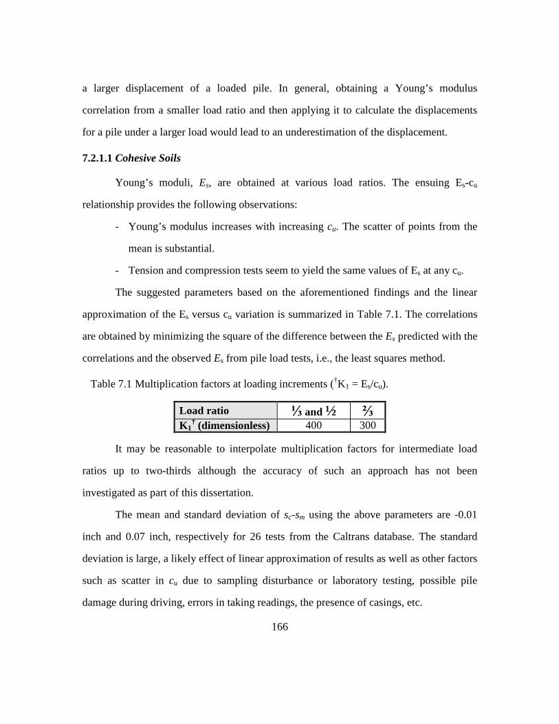
166

a larger displacement of a loaded pile. In general, obtaining a Young’s modulus

correlation from a smaller load ratio and then applying it to calculate the displacements

for a pile under a larger load would lead to an underestimation of the displacement.

7.2.1.1 Cohesive Soils

Young’s moduli, Es, are obtained at various load ratios. The ensuing Es-cu

relationship provides the following observations:

- Young’s modulus increases with increasing cu. The scatter of points from the

mean is substantial.

- Tension and compression tests seem to yield the same values of Es at any cu.

The suggested parameters based on the aforementioned findings and the linear

approximation of the Es versus cu variation is summarized in Table 7.1. The correlations

are obtained by minimizing the square of the difference between the Es predicted with the

correlations and the observed Es from pile load tests, i.e., the least squares method.

Table 7.1 Multiplication factors at loading increments (†K1 = Es/cu).

Load ratio ⅓ and ½ ⅔ K1

† (dimensionless) 400 300

It may be reasonable to interpolate multiplication factors for intermediate load

ratios up to two-thirds although the accuracy of such an approach has not been

investigated as part of this dissertation.

The mean and standard deviation of sc-sm using the above parameters are -0.01

inch and 0.07 inch, respectively for 26 tests from the Caltrans database. The standard

deviation is large, a likely effect of linear approximation of results as well as other factors

such as scatter in cu due to sampling disturbance or laboratory testing, possible pile

damage during driving, errors in taking readings, the presence of casings, etc.

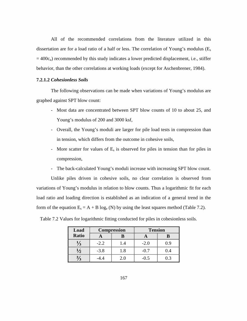
167

All of the recommended correlations from the literature utilized in this

dissertation are for a load ratio of a half or less. The correlation of Young’s modulus (Es

= 400cu) recommended by this study indicates a lower predicted displacement, i.e., stiffer

behavior, than the other correlations at working loads (except for Aschenbrener, 1984).

7.2.1.2 Cohesionless Soils

The following observations can be made when variations of Young’s modulus are

graphed against SPT blow count:

- Most data are concentrated between SPT blow counts of 10 to about 25, and

Young’s modulus of 200 and 3000 ksf,

- Overall, the Young’s moduli are larger for pile load tests in compression than

in tension, which differs from the outcome in cohesive soils,

- More scatter for values of Es is observed for piles in tension than for piles in

compression,

- The back-calculated Young’s moduli increase with increasing SPT blow count.

Unlike piles driven in cohesive soils, no clear correlation is observed from

variations of Young’s modulus in relation to blow counts. Thus a logarithmic fit for each

load ratio and loading direction is established as an indication of a general trend in the

form of the equation Es = A + B loge (N) by using the least squares method (Table 7.2).

Table 7.2 Values for logarithmic fitting conducted for piles in cohesionless soils.

Compression Tension Load Ratio A B A B

⅓ -2.2 1.4 -2.0 0.9

½ -3.8 1.8 -0.7 0.4

⅔ -4.4 2.0 -0.5 0.3

168

When the factors listed above are utilized for the 34 load tests in the Caltrans

database, the mean value of sc-sm is zero while the standard deviation is 0.13 inches. In

addition to the errors in conducting the pile load test, the variability of SPT blow counts

due to applied hammer energy can also be a significant source of error.

7.2.1.3 Suggested Correlations Applied to Piles in Mixed Profiles

Displacements are predicted for 83 piles in the Caltrans database, which are

driven into soils with mixed profiles, using the proposed correlations. None of these piles

was included in the derivation of the suggested correlations. Therefore, these piles

provide an independent means of investigating the applicability of the correlations. The

results indicate a satisfactory outcome for all load ratios (Table 6.3).

Table 7.3 Statistics for settlement ratio (sc/sm) and displacement difference (sc-sm) (N=83).

Statistics (sc/sm) Third Half Two-Thirds Mean, x 1.18 1.02 1.08 Standard Dev., sx 0.60 0.47 0.48 Statistics (sc-sm) (inch) Third Half Two-Thirds

Mean, x 0.01 0.00 -0.01 Standard Dev., sx 0.04 0.07 0.10

7.2.2 Recommendations for Future Work

Cone penetration testing (CPT) has been gaining in popularity for purposes of site

characterization and design. Research based on CPT seems to be improving its use for

characterizing soils in the field with the exception of dense sandy and/or gravelly layers.

Thus, CPT can be utilized to analyze the data collected as part of the Caltrans project.

A natural extension of any developed method for a single pile is towards pile

groups because piles used for support of structures on land (as opposed to offshore)

169

typically are in groups. Unfortunately, none of the Caltrans pile load tests was conducted

on groups of piles although most of the piles were a part of a group.

In areas with gravel and cobbles, often the cone penetrometer cannot be pushed to

the desired depth and SPT blow counts reach refusal as well. For such cases, geophysical

methods such as the Oyo suspension logger or spectral analysis of shear waves (SASW)

would be very useful. To the best of the author’s knowledge, there is a lack of

correlations for estimating displacements of piles in coarse materials, especially gravels

and cobbles.

An integral approach to pile design combining pile capacity with displacement

would bridge the gap in design of piled foundations, where emphasis is usually given to

the capacity.

7.3 OTHER RECOMMENDATIONS

Other analyses methods can be considered:

- Analyses with t-z curves are widely used and may be especially useful for cases

in which load shedding is significant. Moreover, a realistic incorporation of the effects of

residual stresses due to pile driving (Alyahyai, 1987) into the analyses would be a step

towards a more comprehensive explanation of all aspects of pile displacement.

- Numerical approaches such as neural networks and finite element methods with

non-linear models of soil-pile interaction might well be further investigated with positive

results for predicting pile displacement. These might well help characterize the non-linear

behavior of load-displacement curves as failure loads are approached.

170

Appendix A: Pile Load Test Information

Appendix A.1 Coupling of bridge numbers, site names, load test numbers, and other descriptive terms.

Bridge Name City Inter. Route Bent Pile CTID LTN

Pier 2 72 001-01 384 04-0017 Van Duzen River

Bridge Fortuna 101

Pier 3 108 001-02 385

20-0172 Central Cloverdale Underpass Cloverdale 101 3 14 004-02 390

20-0251 Central Cloverdale Undercrossing Cloverdale 101 Abutment 2R 28 004-01 389

006a-01 397 14 (#1)

006a-02 398

006a-03 399 14 (#2)

006a-04 400

10 006a-05 401

14 (#3) 006b-01 402

20-0254 Russian River Bridge Guerneville 116 Pier 3

27 006b-02 403

22-0032 Sacramento River Bypass Bryte 16 Pier 37 2 124L-01 735

22-0062 Mullen Overhead Woodland 113 2R 21 122L-01 736

28-0009 San Joaquin River Bridge Antioch 84 19 15 007-01 404

28-0056 Railroad Ave. Overhead Richmond 17 5L 10 118L-01 788

4 3 002-01 386 28-0249 West Connector

Overcrossing Concord 4/242 8 20 002a-01 387

28-0292 Harbor Way Overcrossing

Richmond 580 Abut. 3 10 003-01 388

22 3 120L-01 790 29-0013 Stanislaus River -

Ripon Modesto 99

6 1 120L-02 762

085-01 675 E28L 17

085-02 676

086-01 677 33-0025 San Francisco-

Oakland Bay Bridge Oakland 80

E31R 1 086-02 678

011-01 455 33-0393 West Grand Avenue

Viaduct Oakland 880 3F 27 011-02 456

009-01 408 13L 8

009-02 409

33-0611 East Bay Viaduct Oakland 880

17R (LT) 17 009-03 410

171


009-04 411

009-05 412 29R 23

009-06 413

012-05 461 10NCI 3

012-06 462

012-03 459 17NCI(LT) 6

012-04 460

012-01 457 27NC(RT) 9

012-02 458

010-01 417

33-0612 Port of Oakland Connector Viaduct Oakland 880/80

31NC(LT) 9 010-02 418

1B 040-01 559

1C 040-02 560

040-03 561

040-04 562 1J

040-05 563

040-06 564 1M

040-07 565

040-08 566 1R

040-09 567

040-10 568

Site 1

1U 040-11 569

029-01 501 2-H

029-02 502

029-03 503 2-L

029-04 504

029-05 505 2-P

029-06 506

029-07 507 2-T

029-08 508

029-09 509

Site 2

2-W 029-10 510

030-01 511 3-C

030-02 512

030-03 513 Site 3

1M 030-04 514

4-B 031-01 515

4-C 031-02 516

I-880 IPTP

I-880 Replacement Project IPTP

Oakland 880

Site 4

4-H 031-03 517

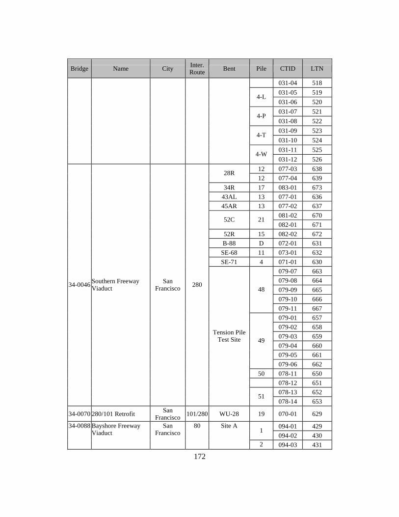
172


031-04 518

031-05 519 4-L

031-06 520

031-07 521 4-P

031-08 522

031-09 523 4-T

031-10 524

031-11 525 4-W

031-12 526

12 077-03 638 28R

12 077-04 639

34R 17 083-01 673

43AL 13 077-01 636

45AR 13 077-02 637

081-02 670 52C 21

082-01 671

52R 15 082-02 672

B-88 D 072-01 631

SE-68 11 073-01 632

SE-71 4 071-01 630

079-07 663

079-08 664

079-09 665

079-10 666

48

079-11 667

079-01 657

079-02 658

079-03 659

079-04 660

079-05 661

49

079-06 662

50 078-11 650

078-12 651

078-13 652

34-0046 Southern Freeway Viaduct

San Francisco

280

Tension Pile Test Site

51 078-14 653

34-0070 280/101 Retrofit San Francisco 101/280 WU-28 19 070-01 629

094-01 429 1

094-02 430

34-0088 Bayshore Freeway Viaduct

San Francisco

80 Site A

2 094-03 431

173


094-04 432

094-05 433 3

094-06 434

095-01 435 1

095-02 436

095-03 437 Site B

2 095-04 438

096-01 439 1

096-02 440

096-03 441 Site C

2 096-04 442

097-01 443 1

097-02 444

097-03 445 Site D

2 097-04 446

098-01 447 1

098-02 448

098-03 449 Site E

2 098-04 450

099-01 451 1

099-02 452

099-03 453 Site F

2 099-04 454

100-01 771 Site G 5

100-02 772

20 14 021-01 478

22, Column 4 4 014-03 470

23, Column 4 5 014-02 469

29, Column 2 19 014-01 468

29, Column 3 4 015-01 471

Site 2 2 019-01 476

3 018-01 475 Site 3

3C 017-01 474

Site 4 4 013-01 463

6 013-02 464 Site 5

7 013-03 465

Site 6 8 013-04 466

34-0100 China Basin Viaduct San Francisco 280

Site 7 10 013-05 467

Pier 04 33 135-01 421 35-0038 Dumbarton Bridge Fremont/ Newark/

84

Pier 16 29 138-02 425

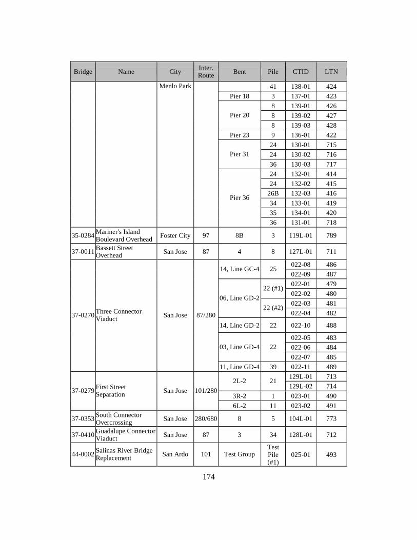
174


41 138-01 424

Pier 18 3 137-01 423

8 139-01 426

8 139-02 427 Pier 20

8 139-03 428

Pier 23 9 136-01 422

24 130-01 715

24 130-02 716 Pier 31

36 130-03 717

24 132-01 414

24 132-02 415

26B 132-03 416

34 133-01 419

35 134-01 420

Menlo Park

Pier 36

36 131-01 718

35-0284 Mariner's Island Boulevard Overhead Foster City 97 8B 3 119L-01 789

37-0011 Bassett Street Overhead San Jose 87 4 8 127L-01 711

022-08 486 14, Line GC-4 25

022-09 487

022-01 479 22 (#1)

022-02 480

022-03 481 06, Line GD-2

22 (#2) 022-04 482

14, Line GD-2 22 022-10 488

022-05 483

022-06 484 03, Line GD-4 22

022-07 485

37-0270 Three Connector Viaduct San Jose 87/280

11, Line GD-4 39 022-11 489

129L-01 713 2L-2 21

129L-02 714

3R-2 1 023-01 490 37-0279 First Street

Separation San Jose 101/280

6L-2 11 023-02 491

37-0353 South Connector Overcrossing San Jose 280/680 8 5 104L-01 773

37-0410 Guadalupe Connector Viaduct San Jose 87 3 34 128L-01 712

44-0002 Salinas River Bridge Replacement San Ardo 101 Test Group

Test Pile (#1)

025-01 493

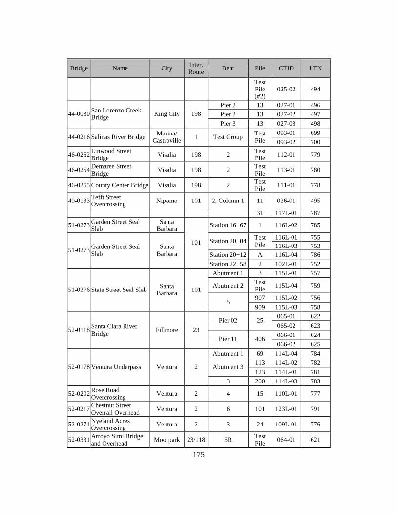
175


Test Pile (#2)

025-02 494

Pier 2 13 027-01 496

Pier 2 13 027-02 497 44-0030 San Lorenzo Creek Bridge King City 198

Pier 3 13 027-03 498

093-01 699 44-0216 Salinas River Bridge Marina/

Castroville 1 Test Group Test Pile 093-02 700

46-0252 Linwood Street Bridge Visalia 198 2 Test

Pile 112-01 779

46-0254 Demaree Street Bridge Visalia 198 2 Test

Pile 113-01 780

46-0255 County Center Bridge Visalia 198 2 Test Pile 111-01 778

49-0133 Tefft Street Overcrossing Nipomo 101 2, Column 1 11 026-01 495

31 117L-01 787

51-0273 Garden Street Seal Slab

Santa Barbara

Station 16+67 1 116L-02 785

116L-01 755 Station 20+04 Test

Pile 116L-03 753 Station 20+12 A 116L-04 786

51-0273 Garden Street Seal Slab

Santa Barbara

101

Station 22+58 2 102L-01 752

Abutment 1 3 115L-01 757

Abutment 2 Test Pile 115L-04 759

907 115L-02 756 51-0276 State Street Seal Slab Santa

Barbara 101

5 909 115L-03 758

065-01 622 Pier 02 25

065-02 623

066-01 624 52-0118 Santa Clara River

Bridge Fillmore 23

Pier 11 406 066-02 625

Abutment 1 69 114L-04 784

113 114L-02 782 Abutment 3

123 114L-01 781 52-0178 Ventura Underpass Ventura 2

3 200 114L-03 783

52-0202 Rose Road Overcrossing

Ventura 2 4 15 110L-01 777

52-0217 Chestnut Street Overrail Overhead

Ventura 2 6 101 123L-01 791

52-0271 Nyeland Acres Overcrossing

Ventura 2 3 24 109L-01 776

52-0331 Arroyo Simi Bridge and Overhead

Moorpark 23/118 5R Test Pile

064-01 621

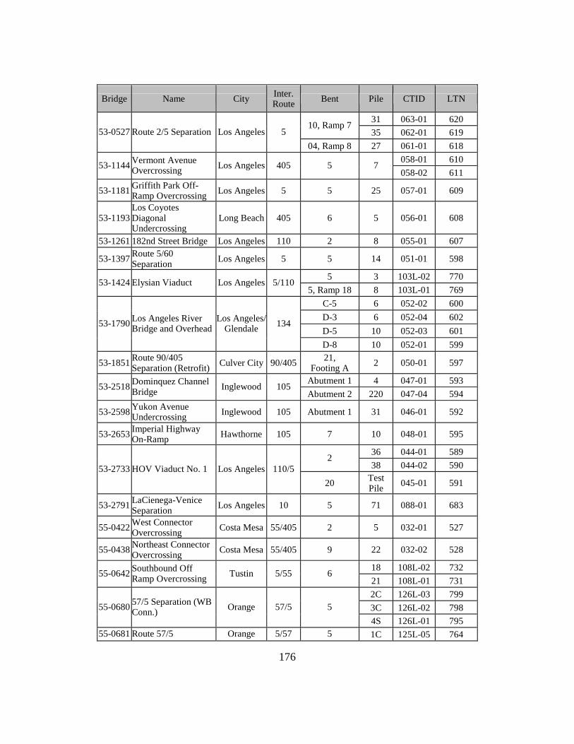
176


31 063-01 620 10, Ramp 7

35 062-01 619 53-0527 Route 2/5 Separation Los Angeles 5

04, Ramp 8 27 061-01 618

058-01 610 53-1144 Vermont Avenue

Overcrossing Los Angeles 405 5 7 058-02 611

53-1181 Griffith Park Off-Ramp Overcrossing Los Angeles 5 5 25 057-01 609

53-1193 Los Coyotes Diagonal Undercrossing

Long Beach 405 6 5 056-01 608

53-1261 182nd Street Bridge Los Angeles 110 2 8 055-01 607

53-1397 Route 5/60 Separation

Los Angeles 5 5 14 051-01 598

5 3 103L-02 770 53-1424 Elysian Viaduct Los Angeles 5/110

5, Ramp 18 8 103L-01 769

C-5 6 052-02 600

D-3 6 052-04 602

D-5 10 052-03 601 53-1790 Los Angeles River

Bridge and Overhead Los Angeles/

Glendale 134

D-8 10 052-01 599

53-1851 Route 90/405 Separation (Retrofit)

Culver City 90/405 21, Footing A

2 050-01 597

Abutment 1 4 047-01 593 53-2518 Dominquez Channel

Bridge Inglewood 105

Abutment 2 220 047-04 594

53-2598 Yukon Avenue Undercrossing Inglewood 105 Abutment 1 31 046-01 592

53-2653 Imperial Highway On-Ramp Hawthorne 105 7 10 048-01 595

36 044-01 589 2

38 044-02 590 53-2733 HOV Viaduct No. 1 Los Angeles 110/5

20 Test Pile

045-01 591

53-2791 LaCienega-Venice Separation

Los Angeles 10 5 71 088-01 683

55-0422 West Connector Overcrossing

Costa Mesa 55/405 2 5 032-01 527

55-0438 Northeast Connector Overcrossing

Costa Mesa 55/405 9 22 032-02 528

18 108L-02 732 55-0642 Southbound Off

Ramp Overcrossing Tustin 5/55 6

21 108L-01 731

2C 126L-03 799

3C 126L-02 798 55-0680 57/5 Separation (WB Conn.) Orange 57/5 5

4S 126L-01 795 55-0681 Route 57/5 Orange 5/57 5 1C 125L-05 764

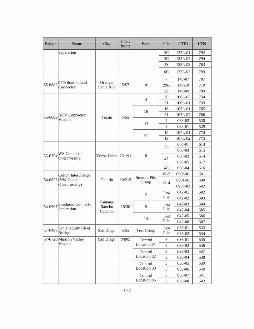
177


2C 125L-01 792

3C 125L-04 794

4S 125L-03 763

Separation

6C 125L-02 793

7 140-07 707

29R 140-10 710 55-0682 57/5 Southbound Connector

Orange/ Santa Ana 5/57 4

38 140-09 709

20 106L-02 734 4

21 106L-01 733

16 105L-01 765 16

21 105L-02 766

2 033-02 530 44

3 033-01 529

15 107L-01 774

55-0689 HOV Connector Viaduct Tustin 5/55

47 19 107L-02 775

060-01 613 23

060-03 615

060-02 614 47

060-05 617

55-0794 WS Connector Overcrossing Yorba Linda 231/91 8

48 060-04 616

#1-2 090b-01 691

090a-01 690 54-0823 Colton Interchange (NW Conn. Overcrossing)

Ontario 10/215 Smooth Pile Group #1-4

090b-02 692

042-01 582 2 Test

Pile 042-02 583

042-03 584 9 Test

Pile 042-04 585

042-05 586

54-0967 Southeast Connector Separation

Fontana/ Rancho Cucamo

15/30

13 Test Pile 042-06 587

035-01 533 57-0488 San Diequito River

Bridge San Diego 5/55 Test Group Test Pile 035-02 534

5 036-01 535 Control Location 01 5 036-02 536



5 036-07 541

57-0720 Mission Valley Viaduct

San Diego 8/805

Control Location 06 5 036-08 542

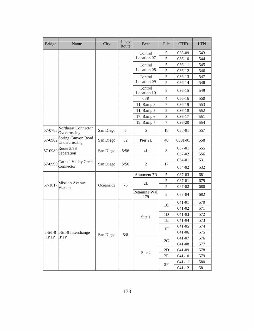
178





Control Location 10 5 036-15 549

03R 4 036-16 550

11, Ramp 3 7 036-19 553

11, Ramp 5 2 036-18 552

17, Ramp 6 3 036-17 551

19, Ramp 7 7 036-20 554

57-0783 Northeast Connector Overcrossing San Diego 5 5 18 038-01 557

57-0982 Spring Canyon Road Undercrossing San Diego 52 Pier 2L 48 039a-01 558

037-01 555 57-0989 Route 5/56

Separation San Diego 5/56 4L 8 037-02 556

034-01 531 57-0990 Carmel Valley Creek

Connector San Diego 5/56 2 17 034-02 532

Abutment 7R 5 087-03 681

5 087-01 679 2L

5 087-02 680 57-1017 Mission Avenue Viaduct Oceanside 76

Retaining Wall 179 5 087-04 682

041-01 570 1C

041-02 571

1D 041-03 572

1E 041-04 573

041-05 574

Site 1

1F 041-06 575

041-07 576 2C

041-08 577

2D 041-09 578

2E 041-10 579

041-11 580

I-5/I-8 IPTP

I-5/I-8 Interchange IPTP San Diego 5/8

Site 2

2F 041-12 581

179

1. “Bridge” is a unique number assigned by Caltrans to each bridge 2. “Bridge Num” is a unique number we assigned to each bridge as we received data

for that structure. It is used as shorthand notation in large tables. 3. “Site” is an abbreviation that brings to mind a site without having to enter a site

description, e.g., Oak is a site in Oakland. The site numbers were assigned for convenience in this report.

4. “Name” is a more general description of the site and structure. 5. “City” is the name of the city within whose borders the site is located. In some

cases it is the name of a nearby city. 6. “County” is the name of the country. 7. “Inter. Route” is the name of an intersecting highway. 8. “Bent” may be an actual bridge bent number or it may be a special term, e.g.,

identification of an abutment. 9. “Pile” is the pile number from the plans for this structure. It is not used further

in this report. 10. “LTN is a load test number assigned by us and used in later tables.

180

Appendix B: Correlations for Young’s Modulus

Appendix B.1 Correlations with Standard Penetration Test (SPT) Blowcount, N.

SPT Soil Type Pile/Found.

Type Es (MPa) Reference Notes/Method

ALL Clays and Sands

All 1.58+0.316N Webb (1970)

All soil 0.835N Ohsaki and Iwasaki (1973)

Clays and sands

All 39.5N0.68

(initial tangent modulus)

Imai & Tonouchi (1982)

Eq. given for G, assumed υ=0.4 (Japanese practice)

All (2.5-2.8)N Shioi & Fukui (1982)

Japanese railway and bridge standards

Clays and Sands

(2.5±0.5)N Decourt et al. (1989)

Pile-soil interface

SPT Soil Type Pile / Found.


COHESIVE/ CLAY

Clays All (0.5±0.2)N Stroud (1974) Below pile tip Clays (0.5 0.2)N± Stroud (1974) Modulus well-below

pile tips, Es(MPa) Clays, bored piles

(0.5 - 0.7)M M =constrained modulus

Stroud (1974) Modulus well-below pile tips, Es(MPa)

Clays All 1.5N Decourt (1978) Clays Driven 3(1+0.16z) /

1.5N Yamashita et al. (1987)

Cast-in-place concrete, side, use the larger value

Clays Driven 3(1+0.16z) Yamashita et al. (1987)

Cast-in-place concrete, tip

Clays Driven (15±5)cu Poulos (1989) Clays All 14N Hirayama

(1991) Small strain

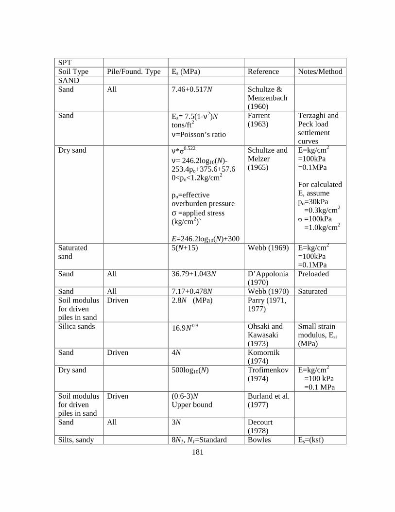
181

SPT Soil Type Pile/Found. Type Es (MPa) Reference Notes/Method SAND Sand All 7.46+0.517N Schultze &

Menzenbach (1960)

Sand Es= 7.5(1-ν2)N tons/ft2

ν=Poisson’s ratio

Farrent (1963)

Terzaghi and Peck load settlement curves

Dry sand ν*σ0.522 ν= 246.2log10(N)- 253.4po+375.6+57.6 0<po<1.2kg/cm2 po=effective overburden pressure σ =applied stress (kg/cm2)` E=246.2log10(N)+300

Schultze and Melzer (1965)

E=kg/cm2 =100kPa =0.1MPa For calculated E, assume po=30kPa =0.3kg/cm2 σ =100kPa =1.0kg/cm2

Saturated sand

5(N+15) Webb (1969) E=kg/cm2 =100kPa =0.1MPa

Sand All 36.79+1.043N D’Appolonia (1970)

Preloaded

Sand All 7.17+0.478N Webb (1970) Saturated Soil modulus for driven piles in sand

Driven 2.8N (MPa) Parry (1971, 1977)

Silica sands 0.916.9N Ohsaki and Kawasaki (1973)

Small strain modulus, Esi

(MPa) Sand Driven 4N Komornik

(1974)

Dry sand 500log10(N) Trofimenkov (1974)

E=kg/cm2 =100 kPa =0.1 MPa

Soil modulus for driven piles in sand

Driven (0.6-3)N Upper bound

Burland et al. (1977)

Sand All 3N Decourt (1978)

Silts, sandy 8N1, N1=Standard Bowles Es=(ksf)

182

SPT Soil Type Pile/Found. Type Es (MPa) Reference Notes/Method SAND silts, slightly cohesive mixtures Clean fine to medium sands and slightly silty sands Coarse sands and sands with little gravel

Penetration Test (SPT) resistance 14N1, N1=Standard Penetration Test (SPT) resistance 20N1, N1=Standard Penetration Test (SPT) resistance

(1982) and U.S. Department of the Navy (1982)

Sand All 7 N Denver (1982)

Average of pressuremeter and screw-plate tests

Silica sands 0.57N Denver (1982)

Modulus well-below pile tips, Es(MPa)

Silica sands, driven piles

0.6153c

q Imai and Tonouchi (1982)


(MPa) Partially saturated sand

2.22N0.888 Wrench and Nowatzki (1985)

E=kg/cm2 =100kPa =0.1MPa

Sand Driven 60+3.2Ns Kurkur (1986)

Ns: average N along shaft. Valid at 50% of failure load.

Sand Driven [ ]6 5 3N + Yamashita et al. (1987)

Cast-in-place concrete, side

Sand Driven 0.4N (30 MPa max.)

Yamashita et al. (1987)

Cast-in-place concrete, tip

Sand 500(N+15) Bowles kPa ( 1

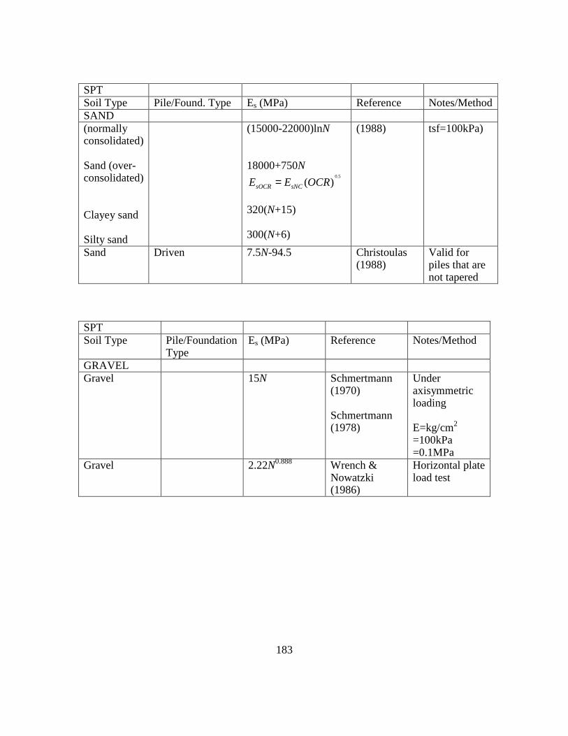
183

SPT Soil Type Pile/Found. Type Es (MPa) Reference Notes/Method SAND (normally consolidated) Sand (over-consolidated) Clayey sand Silty sand

(15000-22000)lnN 18000+750N

0.5

( )sOCR sNCE E OCR= 320(N+15) 300(N+6)

(1988) tsf=100kPa)

Sand Driven 7.5N-94.5 Christoulas (1988)

Valid for piles that are not tapered

SPT Soil Type Pile/Foundation


GRAVEL Gravel 15N Schmertmann

(1970) Schmertmann (1978)

Under axisymmetric loading E=kg/cm2 =100kPa =0.1MPa

Gravel 2.22N0.888 Wrench & Nowatzki (1986)

Horizontal plate load test

184

SPT Soil Type Pile/Foundation


COHESIONLESS Sand to Gravel

Sands and gravel All 18.75+0.756N D’Appolonia (1970)

Normally consolidated sand

Gravel with sand 12(N+6) N<15 40+12(N-6) N>15

Begemann (1974)

E=kg/cm2 =100kPa =0.1MPa

Silt with sand to gravel with sand

40 ( - 6)sE C N= + kg/cm2 N>15

( 6)Es C N= + kg/cm2 C= 3 (silt with sand) to 12 (gravel with sand)

Begemann (1974)

Used in Greece

Sand and gravel Silty sand

/ 2S p B N=

/S p B N= inches p in tons/ft2, B in inches

Meyerhof (1974)

Analysis of field data of Schultze and Sherif (1973) Conservative estimate of maximum settlement of shallow foundations

Sandy gravel and gravels

24N1, N1=Standard Penetration Test (SPT) resistance

Bowles (1982) and U.S. Department of the Navy (1982)

Es=(ksf)

Gravelly sand and gravel

600(N+6) 15N ≤ 600(N+6)+2000 N>15

Bowles (1988)

kPa ( 1 tsf=100kPa)

185

Appendix B.2 Correlations based on cone penetration test (CPT) data

Soil Type Pile/Foun-dation Type

Es (MPa) Reference Notes/Method

ALL All 1.5 cq Buisman

(1940) Very conservative

Pure sand Silty sand Clayey sand Soft clay

s cE qα=

0.8 0.9α = − 1.3 1.9α = − 3.8 5.7α = − 7.7α =

Bachelier and Parez (1965)

All 1.9 /c oC q p= Meyerhof (1965)

Based on back- calculated settlement records

All Es=2qc Schmertmann (1970)

Screw plate tests used to measure E

Clayey sand 2.4+1.67qc Webb (1970) Saturated All E= function of both

cone resistance and overburden pressure

Folque (1974)

All p net aE m q q=

qa=ref stress =100 kPa

netq =net cone resistance

Janbu (1974) mp is determined from Nq value

All 1.141 33.129cE q= + (E in kg/cm2)

Schultze (1974)

Based on laboratory tests

Sands Clays

3s cE q=

7s cE q=

Trofimenkov (1974)

U.S.S.R. practice

All cqα , 3 10α< < Veismanis

(1974) Txl tests and penetration tests in small chamber

Unspecified st cE qα=

10.8 6.6s cE q= +

Holeyman (1985) Verbrugge (1982)

α =24-30 Dynamic modulus value

sE and cq in

186

Soil Type Pile/Foun-dation Type

Es (MPa) Reference Notes/Method

ALL MN/m2 (for

cq >0.4MN/m2)

Clays and sands

All 21.066qc1.091 Christoulas

(1988)

Silica sands, driven piles Clays, driven piles

(7.5 2.5) cq± (7.5 2.5) cq±

Poulos (1989) Stroud (1974)

Near-shaft modulus, Es

(MPa) Modulus well-below pile tips, Es(MPa)

Soil Type Pile/Foundation


CLAY Clays, driven piles

(500 5) cq± Callanan and Kulhawy (1985)


(MPa)

Clays (150-225)cu

200 Johnson (1986)

Clays (3-8)qc Johnson (1986) Clay and silts * 1.0921.0

s cE q=

sE =15 cq

Christoulas (1988) Poulos (1988c)

Various pile types sE and

cq in MN/m2

*sE = secant

Young’s modulus

Clays, bored piles

10 cq Christoulas and Frank (1991)


(MPa) Clays, driven piles

0.695 1.13049.4 cq e− Mayne and Rix

(1993) Small strain modulus, Esi

(MPa)

187

Soil Type Es (MPa) Reference Notes/Method SAND Sands 1.5s cE q= Buisman

(1940) Overpredicts settlements by a factor of about two

NC Sands 1.5qc De Beer & Martens (1957)

Sand 2.5sE qc=

100 5s cE q= +

Trofimenkov (1964)

Lower limit Average

Sand 1.9qc Meyerhof (1965)

Dry sand .5521E v

mvσ= =

2

301.1log 382.3

60.3 50.3 /

cv q

log cm

γ= − +

±

Shultze and Melzer (1965)

Compacted in 3m diameter test pit

Sand 22(1 )r cE D q= + , Dr=rel. density

Vesic (1965) Pile load tests in sand

Sand 1.5s cE q= De Beer (1967)

Overpredicts settlements by a factor of two

Overconsolidated sand

( / )oed oedA C A C= De Beer (1967)

C from field tests

oedA and oedC from lab oedometer tests

2.3(1 ) /oed cC e C= +

2.3(1 ) /oed sA e C= +

Normally consolidated sands

s cE qα=

3 12α = −

Thomas (1968)

Based on penetration and compression tests in large chambers Lower values of α at higher values of cq ; attributed to grain crushing

Sands 22.5 75 /cE q ton ft= + Webb (1969) Plate load tests on sands. E values checked with observed settlements

Sands 2qc Schmertmann Based on screw plate

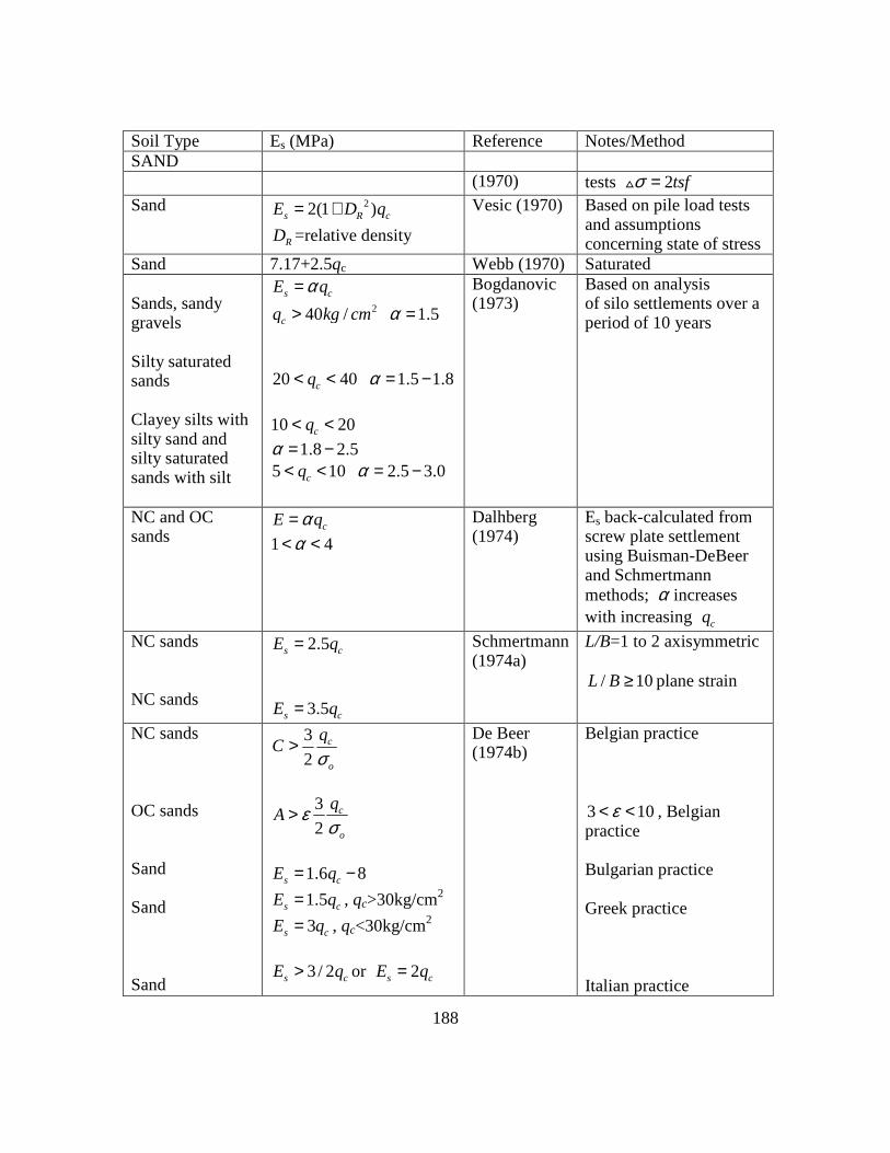
188

Soil Type Es (MPa) Reference Notes/Method SAND

(1970) tests 2tsfσ =△ Sand 22(1 )s R cE D q= +

RD =relative density

Vesic (1970) Based on pile load tests and assumptions concerning state of stress

Sand 7.17+2.5qc Webb (1970) Saturated Sands, sandy gravels Silty saturated sands Clayey silts with silty sand and silty saturated sands with silt

s cE qα= 240 /cq kg cm> 1.5α =

20 40cq< < 1.5 1.8α = − 10 20cq< <

1.8 2.5α = − 5 10cq< < 2.5 3.0α = −

Bogdanovic (1973)

Based on analysis of silo settlements over a period of 10 years

NC and OC sands

cE qα=

1 4α< <

Dalhberg (1974)

Es back-calculated from screw plate settlement using Buisman-DeBeer and Schmertmann methods; α increases with increasing cq

NC sands NC sands

2.5s cE q=

3.5s cE q=

Schmertmann (1974a)

L/B=1 to 2 axisymmetric

/ 10L B ≥ plane strain

NC sands OC sands Sand Sand Sand

3

2c

o

qC

σ>

3

2c

o

qA ε

σ>

1.6 8s cE q= −

1.5s cE q= , qc>30kg/cm2

3s cE q= , qc<30kg/cm2

3 / 2s cE q> or 2s cE q=

De Beer (1974b)

Belgian practice 3 10ε< < , Belgian practice Bulgarian practice Greek practice Italian practice

189

Soil Type Es (MPa) Reference Notes/Method SAND Sand Fine to medium sand Clayey sands, PI<15% Sands

1.9s cE q=

25( 3200) /

2s cE q kN m= +

25( 1600) /

3s cE q kN m= +

s cE qα= , 1.5 2α< <

South African practice U.K. practice

Sands 2.5qc Schmertmann (1978)

Modified, axisymmetrical footing

Sands 8

0

cqq

Denver (1982)

q0 = 1 MPa, 1.3CPT Dutchconeq q =

Silica Sands s cE qα=

† 0.6153st cE q=

Milovic and Stevanovic (1982) Poulos (1988c) Imai and Tonouchi (1982)

α =20-40 α =5 (normally-consolidated sands) α =7.5 (over-consolidated sands)

stE and cq in MN/m2

Dynamic modulus value †

stE =initial tangent

Young’s modulus

Sandy soils 4 cq Bowles (1982) and U.S. Department of the Navy (1982)

cq =Cone penetration resistance (ksf)

Sand (normally 2 – 4 qc Bowles kPa ( 1 tsf=100kPa)

190

Soil Type Es (MPa) Reference Notes/Method SAND consolidated) Sand (over-consolidated) Clayey sand Silty sand Soft clay

2(1 )r cD q+

6-30 qc

3-6qc

1-2qc

3-8qc

(1988)

Silica sands, driven piles

(7 4) cq± Jamiolkowski et al. (1988)

Modulus well-below pile tips, Es(MPa)

Silica, bored piles

(3 0.5) cq± Poulos (1993)


(MPa) Soil Type Pile/Foundation


COHESIONLESS Sand to Gravel

Cohesionless soil / 2 cS pB q= in consistent units S=settlement

Meyerhof (1974)

Conservative estimate, based on analysis of vertical strain

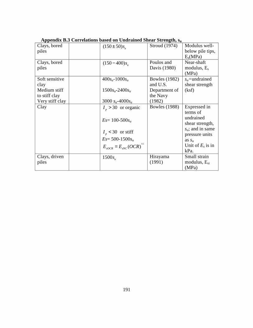
191

Appendix B.3 Correlations based on Undrained Shear Strength, su Clays, bored piles

(150 50) us± Stroud (1974) Modulus well-below pile tips, Es(MPa)

Clays, bored piles

(150 400)us− Poulos and Davis (1980)


(MPa) Soft sensitive clay Medium stiff to stiff clay Very stiff clay

400su-1000su

1500su-2400su

3000 su-4000su

Bowles (1982) and U.S. Department of the Navy (1982)

su=undrained shear strength (ksf)

Clay 30pI > or organic

Es= 100-500su

30pI < or stiff

Es= 500-1500su 0.5

( )sOCR sNCE E OCR=

Bowles (1988) Expressed in terms of undrained shear strength, su; and in same pressure units as su Unit of Es is in kPa.

Clays, driven piles

1500 us Hirayama (1991)


(MPa)

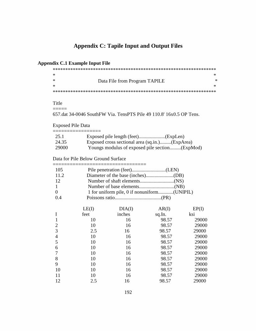
192

Appendix C: Tapile Input and Output Files

Appendix C.1 Example Input File *************************************************** ************** * * * Data File from Program TAPILE * * * *************************************************** ************** Title ===== 657.dat 34-0046 SouthFW Via. TensPTS Pile 49 110.8' 16x0.5 OP Tens. Exposed Pile Data ================= 25.1 Exposed pile length (feet).....................(ExpLen) 24.35 Exposed cross sectional area (sq.in.).........(ExpArea) 29000 Youngs modulus of exposed pile section.........(ExpMod) Data for Pile Below Ground Surface ================================= 105 Pile penetration (feet)...........................(LEN) 11.2 Diameter of the base (inches)......................(DB) 12 Number of shaft elements...........................(NS) 1 Number of base elements............................(NB) 0 1 for uniform pile, 0 if nonuniform............(UNIPIL) 0.4 Poissons ratio.....................................(PR) LE(I) DIA(I) AR(I) EP(I) I feet inches sq.In. ksi 1 10 16 98.57 29000 2 10 16 98.57 29000 3 2.5 16 98.57 29000 4 10 16 98.57 29000 5 10 16 98.57 29000 6 10 16 98.57 29000 7 10 16 98.57 29000 8 10 16 98.57 29000 9 10 16 98.57 29000 10 10 16 98.57 29000 11 10 16 98.57 29000 12 2.5 16 98.57 29000

193

Data for Soil ============= 0 0 for nonuniform soil,1 for uniform soil........(IUNIF) Layer Youngs Modulus (ksf) 1 0.001 2 0.001 3 394 4 636 5 636 6 636 7 636 8 636 9 636 10 636 11 636 12 636 13 636 1212 Youngs modulus of soil below the pile tip(ksf)..(EBase) 115 Thickness of soil (feet)........................(SoilH) Side Shear Stresses at Failure in Compression ============================================ 0.001 side shear at failure in compression (ksf).....[TA(1)] 0.001 side shear at failure in compression (ksf).....[TA(2)] 0.858 side shear at failure in compression (ksf).....[TA(3)] 0.904 side shear at failure in compression (ksf).....[TA(4)] 0.904 side shear at failure in compression (ksf).....[TA(5)] 0.904 side shear at failure in compression (ksf).....[TA(6)] 0.904 side shear at failure in compression (ksf).....[TA(7)] 0.904 side shear at failure in compression (ksf).....[TA(8)] 0.904 side shear at failure in compression (ksf).....[TA(9)] 0.904 side shear at failure in compression (ksf).....[TA(10)] 0.904 side shear at failure in compression (ksf).....[TA(11)] 0.904 side shear at failure in compression (ksf).....[TA(12)] End Bearing Stresses in Compression =================================== 9.436 tip failure stress in compression (ksf)........[TA(13)] Side Shear Stresses at Failure in Tension ========================================= 0.001 side shear at failure in tension (ksf).......[TAUP(1)] 0.001 side shear at failure in tension (ksf).......[TAUP(2)]

194

0.807 side shear at failure in tension (ksf).......[TAUP(3)] 0.85 side shear at failure in tension (ksf).......[TAUP(4)] 0.85 side shear at failure in tension (ksf).......[TAUP(5)] 0.85 side shear at failure in tension (ksf).......[TAUP(6)] 0.85 side shear at failure in tension (ksf).......[TAUP(7)] 0.85 side shear at failure in tension (ksf).......[TAUP(8)] 0.85 side shear at failure in tension (ksf).......[TAUP(9)] 0.85 side shear at failure in tension (ksf).......[TAUP(10)] 0.85 side shear at failure in tension (ksf).......[TAUP(11)] 0.85 side shear at failure in tension (ksf).......[TAUP(12)] Tip Tensile Stresses at Failure =============================== 0.001 tip failure stress in tension (ksf)..........[TAUP(13)] Loads ===== 16 Number of loads.................................(Loads) -20 Total applied load (kips).....................[PSum(1)] -40 Total applied load (kips).....................[PSum(2)] -60 Total applied load (kips).....................[PSum(3)] -80 Total applied load (kips).....................[PSum(4)] -100.77 Total applied load (kips).....................[PSum(5)] -120 Total applied load (kips).....................[PSum(6)] -140 Total applied load (kips).....................[PSum(7)] -151.16 Total applied load (kips).....................[PSum(8)] -160 Total applied load (kips).....................[PSum(9)] -180 Total applied load (kips).....................[PSum(10)] -201.55 Total applied load (kips).....................[PSum(11)] -220 Total applied load (kips).....................[PSum(12)] -240 Total applied load (kips).....................[PSum(13)] -260 Total applied load (kips).....................[PSum(14)] -280 Total applied load (kips).....................[PSum(15)] -302.22 Total applied load (kips).....................[PSum(16)] Data for Measured Load-Settlement Curve ======================================= 0 =number of points on measured Q-S curve (MeasPts)

195

Appendix C.2 Example Output File *************************************************** ************* * * * Output from Program TAPILE * * * *************************************************** ************* Analysis performed on 7/ 3/2006 at 22:46 Title ===== 657.dat 34-0046 SouthFW Via. TensPTS Pile 49 110.8' 16x0.5 OP Tens. Input Data ========== Exposed Length.............(ExpLen) 25.10 feet Exposed Area..............(ExpArea) 24.4 sq.in. Exposed Modulus............(ExpMod) 29000. ksi Pile Penetration..............(LEN) 105.00 feet Base Diameter..................(DB) 11.20 inches Pile Poissons Ratio............(PR) 0.40 Number of Side Elements........(NS) 12 Number of Base Elements........(NB) 1 Number of Discontinuities......(ND) 0 Element Length Diameter Pile Modulus Section Area Num. feet inches ksi sq.in. 1 10.00 16.00 29000. 98.57 2 10.00 16.00 29000. 98.57 3 2.50 16.00 29000. 98.57 4 10.00 16.00 29000. 98.57 5 10.00 16.00 29000. 98.57 6 10.00 16.00 29000. 98.57 7 10.00 16.00 29000. 98.57 8 10.00 16.00 29000. 98.57 9 10.00 16.00 29000. 98.57 10 10.00 16.00 29000. 98.57 11 10.00 16.00 29000. 98.57 12 2.50 16.00 29000. 98.57 Element Soil Modulus Num. ksf 1 0. 2 0. 3 394.

196

4 636. 5 636. 6 636. 7 636. 8 636. 9 636. 10 636. 11 636. 12 636. 13 636. Total Depth of Soil (feet).......... 115.00 feet Modulus of Sublayer................. 1212.00 ksf Ultimate Load in Compression........ 327.92 kips Ultimate Load in Tension............ 302.27 kips Side Shearing Stresses Element Compression Tension Num ksf ksf 1 0.001 0.001 2 0.001 0.001 3 0.858 0.807 4 0.904 0.850 5 0.904 0.850 6 0.904 0.850 7 0.904 0.850 8 0.904 0.850 9 0.904 0.850 10 0.904 0.850 11 0.904 0.850 12 0.904 0.850 Tip Stresses Element Compression Tension Num ksf ksf 13 9.44 0.00 Tip Stresses for Discontinuities Element Compression Tension Num ksf ksf **************************************** Load Number 1 Load Increment....... -20.00 Total Load........... -20.00

197

Element Side Shearing Movement No. Stress, ksf inch 1 0.0000 -0.0115 2 0.0000 -0.0106 3 -0.0695 -0.0101 4 -0.0758 -0.0096 5 -0.0598 -0.0089 6 -0.0539 -0.0084 7 -0.0503 -0.0079 8 -0.0481 -0.0075 9 -0.0469 -0.0072 10 -0.0478 -0.0070 11 -0.0528 -0.0069 12 -0.0978 -0.0068 13 -0.0010 -0.0068 Compression of exposed pile -0.0085 inch Compression of immersed pile -0.0119 inch Depth Load feet kips 0.00 -20.00 10.00 -20.00 20.00 -20.00 22.50 -19.27 32.50 -16.09 42.50 -13.59 52.50 -11.33 62.50 -9.22 72.50 -7.21 82.50 -5.24 92.50 -3.24 102.50 -1.03 105.00 0.00 **************************************** Load Number 2 Load Increment....... -20.00 Total Load........... -40.00 Element Side Shearing Movement No. Stress, ksf inch 1 0.0000 -0.0229 2 0.0000 -0.0213

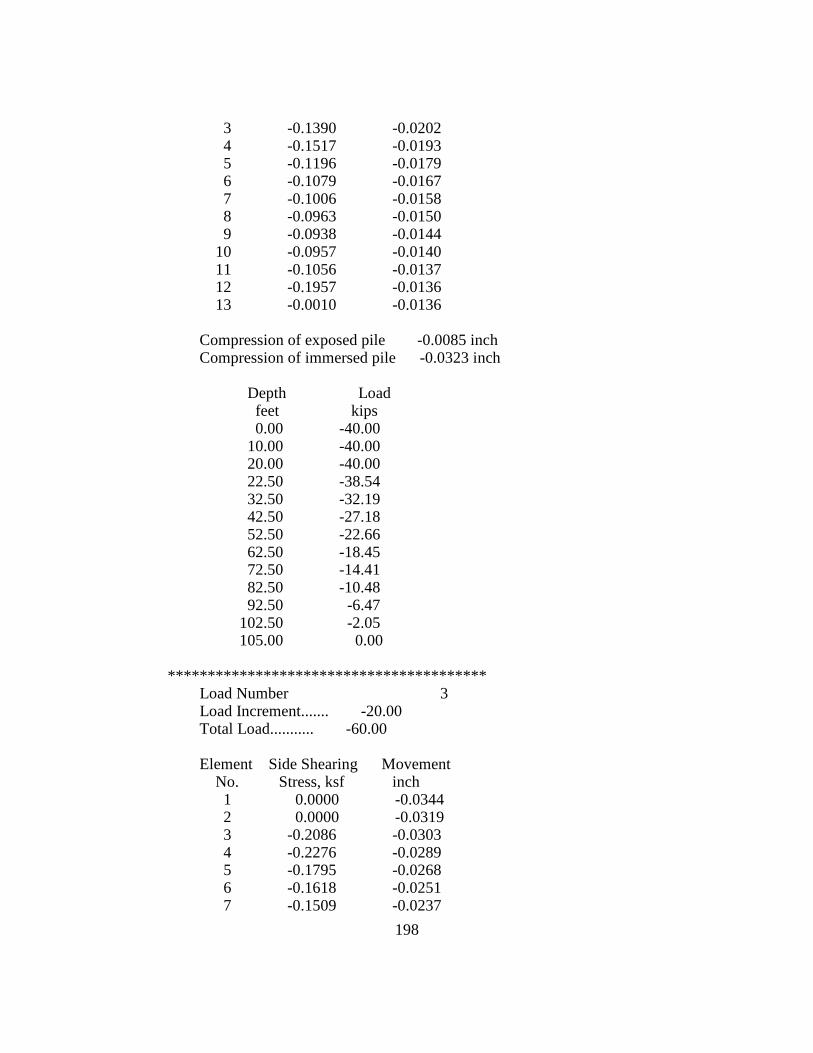
198

3 -0.1390 -0.0202 4 -0.1517 -0.0193 5 -0.1196 -0.0179 6 -0.1079 -0.0167 7 -0.1006 -0.0158 8 -0.0963 -0.0150 9 -0.0938 -0.0144 10 -0.0957 -0.0140 11 -0.1056 -0.0137 12 -0.1957 -0.0136 13 -0.0010 -0.0136 Compression of exposed pile -0.0085 inch Compression of immersed pile -0.0323 inch Depth Load feet kips 0.00 -40.00 10.00 -40.00 20.00 -40.00 22.50 -38.54 32.50 -32.19 42.50 -27.18 52.50 -22.66 62.50 -18.45 72.50 -14.41 82.50 -10.48 92.50 -6.47 102.50 -2.05 105.00 0.00 **************************************** Load Number 3 Load Increment....... -20.00 Total Load........... -60.00 Element Side Shearing Movement No. Stress, ksf inch 1 0.0000 -0.0344 2 0.0000 -0.0319 3 -0.2086 -0.0303 4 -0.2276 -0.0289 5 -0.1795 -0.0268 6 -0.1618 -0.0251 7 -0.1509 -0.0237

199

8 -0.1445 -0.0225 9 -0.1407 -0.0216 10 -0.1435 -0.0210 11 -0.1584 -0.0206 12 -0.2936 -0.0204 13 -0.0010 -0.0204 Compression of exposed pile -0.0085 inch Compression of immersed pile -0.0527 inch Depth Load feet kips 0.00 -60.00 10.00 -60.00 20.00 -60.00 22.50 -57.82 32.50 -48.28 42.50 -40.77 52.50 -33.99 62.50 -27.67 72.50 -21.62 82.50 -15.72 92.50 -9.71 102.50 -3.08 105.00 0.00 **************************************** Load Number 4 Load Increment....... -20.00 Total Load........... -80.00 Element Side Shearing Movement No. Stress, ksf inch 1 0.0000 -0.0459 2 0.0000 -0.0425 3 -0.2781 -0.0404 4 -0.3034 -0.0385 5 -0.2393 -0.0358 6 -0.2158 -0.0335 7 -0.2012 -0.0316 8 -0.1926 -0.0300 9 -0.1876 -0.0288 10 -0.1913 -0.0279 11 -0.2112 -0.0274 12 -0.3915 -0.0272

200

13 -0.0010 -0.0272 Compression of exposed pile -0.0085 inch Compression of immersed pile -0.0731 inch Depth Load feet kips 0.00 -80.00 10.00 -80.00 20.00 -80.00 22.50 -77.09 32.50 -64.38 42.50 -54.36 52.50 -45.32 62.50 -36.89 72.50 -28.82 82.50 -20.96 92.50 -12.95 102.50 -4.10 105.00 0.00 **************************************** Load Number 5 Load Increment....... -20.77 Total Load........... -100.77 Element Side Shearing Movement No. Stress, ksf inch 1 0.0000 -0.0578 2 0.0000 -0.0535 3 -0.3503 -0.0509 4 -0.3822 -0.0485 5 -0.3014 -0.0451 6 -0.2718 -0.0422 7 -0.2534 -0.0398 8 -0.2426 -0.0378 9 -0.2364 -0.0363 10 -0.2410 -0.0352 11 -0.2661 -0.0345 12 -0.4931 -0.0343 13 -0.0010 -0.0343 Compression of exposed pile -0.0089 inch Compression of immersed pile -0.0940 inch

201

Depth Load feet kips 0.00 -100.77 10.00 -100.77 20.00 -100.77 22.50 -97.10 32.50 -81.09 42.50 -68.47 52.50 -57.08 62.50 -46.47 72.50 -36.31 82.50 -26.41 92.50 -16.31 102.50 -5.16 105.00 0.00 **************************************** Load Number 6 Load Increment....... -19.23 Total Load........... -120.00 Element Side Shearing Movement No. Stress, ksf inch 1 0.0000 -0.0688 2 0.0000 -0.0638 3 -0.4171 -0.0606 4 -0.4551 -0.0578 5 -0.3589 -0.0537 6 -0.3237 -0.0502 7 -0.3018 -0.0474 8 -0.2889 -0.0450 9 -0.2815 -0.0432 10 -0.2870 -0.0419 11 -0.3169 -0.0411 12 -0.5872 -0.0408 13 -0.0010 -0.0408 Compression of exposed pile -0.0082 inch Compression of immersed pile -0.1143 inch Depth Load feet kips 0.00 -120.00 10.00 -120.00 20.00 -120.00

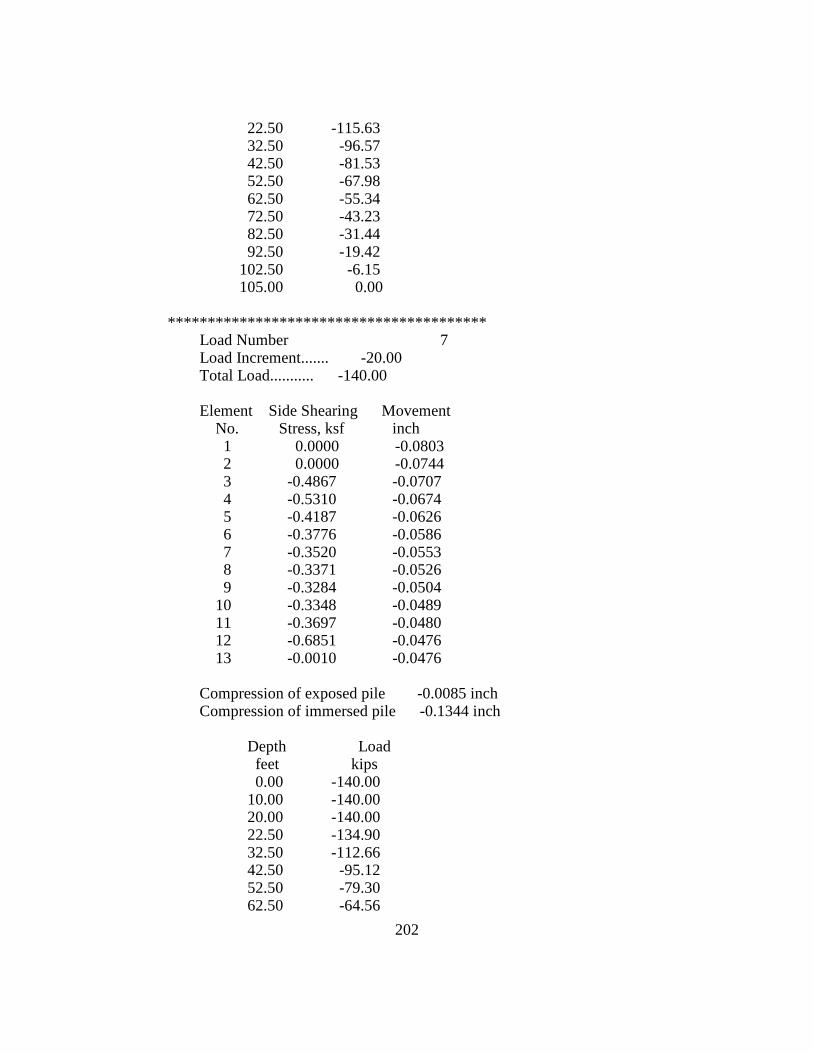
202

22.50 -115.63 32.50 -96.57 42.50 -81.53 52.50 -67.98 62.50 -55.34 72.50 -43.23 82.50 -31.44 92.50 -19.42 102.50 -6.15 105.00 0.00 **************************************** Load Number 7 Load Increment....... -20.00 Total Load........... -140.00 Element Side Shearing Movement No. Stress, ksf inch 1 0.0000 -0.0803 2 0.0000 -0.0744 3 -0.4867 -0.0707 4 -0.5310 -0.0674 5 -0.4187 -0.0626 6 -0.3776 -0.0586 7 -0.3520 -0.0553 8 -0.3371 -0.0526 9 -0.3284 -0.0504 10 -0.3348 -0.0489 11 -0.3697 -0.0480 12 -0.6851 -0.0476 13 -0.0010 -0.0476 Compression of exposed pile -0.0085 inch Compression of immersed pile -0.1344 inch Depth Load feet kips 0.00 -140.00 10.00 -140.00 20.00 -140.00 22.50 -134.90 32.50 -112.66 42.50 -95.12 52.50 -79.30 62.50 -64.56

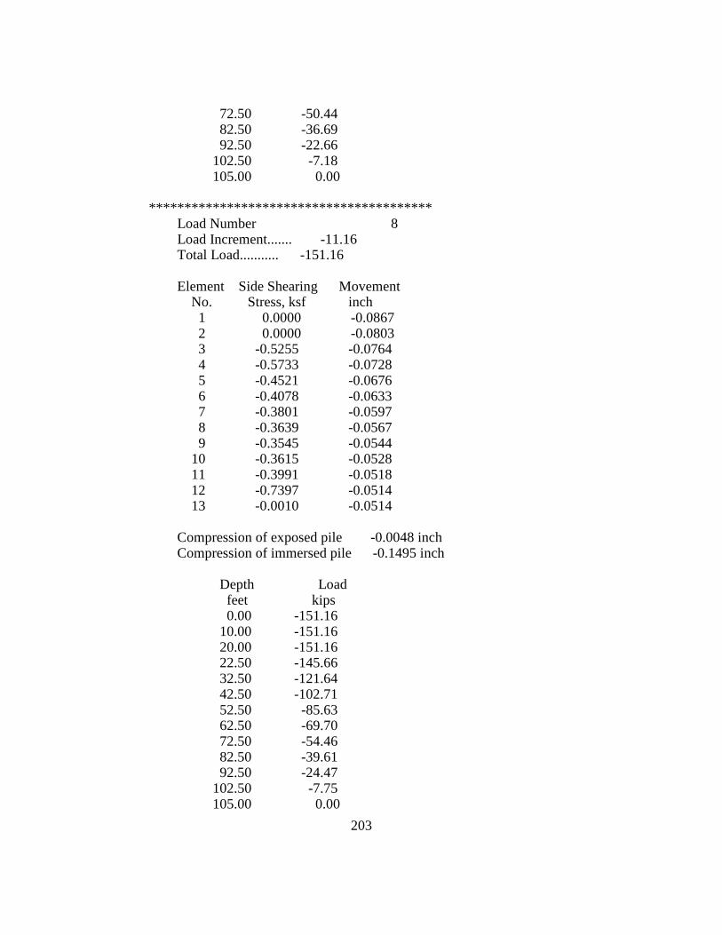
203

72.50 -50.44 82.50 -36.69 92.50 -22.66 102.50 -7.18 105.00 0.00 **************************************** Load Number 8 Load Increment....... -11.16 Total Load........... -151.16 Element Side Shearing Movement No. Stress, ksf inch 1 0.0000 -0.0867 2 0.0000 -0.0803 3 -0.5255 -0.0764 4 -0.5733 -0.0728 5 -0.4521 -0.0676 6 -0.4078 -0.0633 7 -0.3801 -0.0597 8 -0.3639 -0.0567 9 -0.3545 -0.0544 10 -0.3615 -0.0528 11 -0.3991 -0.0518 12 -0.7397 -0.0514 13 -0.0010 -0.0514 Compression of exposed pile -0.0048 inch Compression of immersed pile -0.1495 inch Depth Load feet kips 0.00 -151.16 10.00 -151.16 20.00 -151.16 22.50 -145.66 32.50 -121.64 42.50 -102.71 52.50 -85.63 62.50 -69.70 72.50 -54.46 82.50 -39.61 92.50 -24.47 102.50 -7.75 105.00 0.00

204

**************************************** Load Number 9 Load Increment....... -8.84 Total Load........... -160.00 Element Side Shearing Movement No. Stress, ksf inch 1 0.0000 -0.0917 2 0.0000 -0.0850 3 -0.5562 -0.0808 4 -0.6068 -0.0770 5 -0.4785 -0.0716 6 -0.4316 -0.0670 7 -0.4023 -0.0632 8 -0.3852 -0.0601 9 -0.3753 -0.0576 10 -0.3826 -0.0559 11 -0.4225 -0.0548 12 -0.7830 -0.0544 13 -0.0010 -0.0544 Compression of exposed pile -0.0038 inch Compression of immersed pile -0.1596 inch Depth Load feet kips 0.00 -160.00 10.00 -160.00 20.00 -160.00 22.50 -154.18 32.50 -128.76 42.50 -108.71 52.50 -90.63 62.50 -73.78 72.50 -57.65 82.50 -41.93 92.50 -25.90 102.50 -8.20 105.00 0.00 **************************************** Load Number 10 Load Increment....... -20.00 Total Load........... -180.00

205

Element Side Shearing Movement No. Stress, ksf inch 1 0.0000 -0.1033 2 0.0000 -0.0957 3 -0.6258 -0.0910 4 -0.6832 -0.0868 5 -0.5388 -0.0806 6 -0.4861 -0.0755 7 -0.4532 -0.0712 8 -0.4338 -0.0677 9 -0.4229 -0.0650 10 -0.4314 -0.0630 11 -0.4787 -0.0618 12 -0.8500 -0.0614 13 -0.0010 -0.0613 Compression of exposed pile -0.0085 inch Compression of immersed pile -0.1753 inch Depth Load feet kips 0.00 -180.00 10.00 -180.00 20.00 -180.00 22.50 -173.45 32.50 -144.83 42.50 -122.26 52.50 -101.90 62.50 -82.92 72.50 -64.74 82.50 -47.03 92.50 -28.96 102.50 -8.90 105.00 0.00 **************************************** Load Number 11 Load Increment....... -21.55 Total Load........... -201.55 Element Side Shearing Movement No. Stress, ksf inch 1 0.0000 -0.1160 2 0.0000 -0.1075

206

3 -0.7011 -0.1022 4 -0.7668 -0.0975 5 -0.6049 -0.0906 6 -0.5459 -0.0848 7 -0.5093 -0.0800 8 -0.4874 -0.0761 9 -0.4760 -0.0731 10 -0.4862 -0.0709 11 -0.5474 -0.0696 12 -0.8500 -0.0692 13 -0.0010 -0.0691 Compression of exposed pile -0.0092 inch Compression of immersed pile -0.1970 inch Depth Load feet kips 0.00 -201.55 10.00 -201.55 20.00 -201.55 22.50 -194.21 32.50 -162.09 42.50 -136.75 52.50 -113.88 62.50 -92.55 72.50 -72.13 82.50 -52.20 92.50 -31.83 102.50 -8.90 105.00 0.00 **************************************** Load Number 12 Load Increment....... -18.45 Total Load........... -220.00 Element Side Shearing Movement No. Stress, ksf inch 1 0.0000 -0.1268 2 0.0000 -0.1176 3 -0.7656 -0.1119 4 -0.8385 -0.1066 5 -0.6614 -0.0991 6 -0.5971 -0.0928 7 -0.5573 -0.0876

207

8 -0.5333 -0.0834 9 -0.5214 -0.0801 10 -0.5330 -0.0777 11 -0.6062 -0.0763 12 -0.8500 -0.0758 13 -0.0010 -0.0758 Compression of exposed pile -0.0079 inch Compression of immersed pile -0.2174 inch Depth Load feet kips 0.00 -220.00 10.00 -220.00 20.00 -220.00 22.50 -211.98 32.50 -176.86 42.50 -149.16 52.50 -124.14 62.50 -100.80 72.50 -78.46 82.50 -56.62 92.50 -34.29 102.50 -8.90 105.00 0.00 **************************************** Load Number 13 Load Increment....... -20.00 Total Load........... -240.00 Element Side Shearing Movement No. Stress, ksf inch 1 0.0000 -0.1397 2 0.0000 -0.1297 3 -0.8070 -0.1234 4 -0.8500 -0.1177 5 -0.7488 -0.1094 6 -0.6634 -0.1025 7 -0.6177 -0.0967 8 -0.5900 -0.0920 9 -0.5775 -0.0884 10 -0.5900 -0.0858 11 -0.6780 -0.0843 12 -0.8500 -0.0838

208

13 -0.0010 -0.0837 Compression of exposed pile -0.0085 inch Compression of immersed pile -0.2386 inch Depth Load feet kips 0.00 -240.00 10.00 -240.00 20.00 -240.00 22.50 -231.55 32.50 -195.94 42.50 -164.58 52.50 -136.79 62.50 -110.92 72.50 -86.20 82.50 -62.01 92.50 -37.30 102.50 -8.90 105.00 0.00 **************************************** Load Number 14 Load Increment....... -20.00 Total Load........... -260.00 Element Side Shearing Movement No. Stress, ksf inch 1 0.0000 -0.1530 2 0.0000 -0.1421 3 -0.8070 -0.1353 4 -0.8500 -0.1290 5 -0.8435 -0.1200 6 -0.7331 -0.1123 7 -0.6807 -0.1060 8 -0.6489 -0.1009 9 -0.6356 -0.0970 10 -0.6488 -0.0941 11 -0.7522 -0.0925 12 -0.8500 -0.0919 13 -0.0010 -0.0919 Compression of exposed pile -0.0085 inch Compression of immersed pile -0.2608 inch

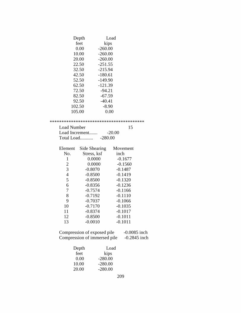
209

Depth Load feet kips 0.00 -260.00 10.00 -260.00 20.00 -260.00 22.50 -251.55 32.50 -215.94 42.50 -180.61 52.50 -149.90 62.50 -121.39 72.50 -94.21 82.50 -67.59 92.50 -40.41 102.50 -8.90 105.00 0.00 **************************************** Load Number 15 Load Increment....... -20.00 Total Load........... -280.00 Element Side Shearing Movement No. Stress, ksf inch 1 0.0000 -0.1677 2 0.0000 -0.1560 3 -0.8070 -0.1487 4 -0.8500 -0.1419 5 -0.8500 -0.1320 6 -0.8356 -0.1236 7 -0.7574 -0.1166 8 -0.7192 -0.1110 9 -0.7037 -0.1066 10 -0.7170 -0.1035 11 -0.8374 -0.1017 12 -0.8500 -0.1011 13 -0.0010 -0.1011 Compression of exposed pile -0.0085 inch Compression of immersed pile -0.2845 inch Depth Load feet kips 0.00 -280.00 10.00 -280.00 20.00 -280.00

210

22.50 -271.55 32.50 -235.94 42.50 -200.34 52.50 -165.34 62.50 -133.61 72.50 -103.49 82.50 -74.01 92.50 -43.98 102.50 -8.90 105.00 0.00 **************************************** Load Number 16 Load Increment....... -22.22 Total Load........... -302.22 Element Side Shearing Movement No. Stress, ksf inch 1 0.0000 -0.1912 2 0.0000 -0.1785 3 -0.8070 -0.1706 4 -0.8500 -0.1632 5 -0.8500 -0.1524 6 -0.8500 -0.1430 7 -0.8500 -0.1352 8 -0.8500 -0.1288 9 -0.8507 -0.1240 10 -0.8500 -0.1206 11 -0.8500 -0.1187 12 -0.8500 -0.1182 13 -0.0010 -0.1181 Compression of exposed pile -0.0095 inch Compression of immersed pile -0.3169 inch Depth Load feet kips 0.00 -302.22 10.00 -302.22 20.00 -302.22 22.50 -293.77 32.50 -258.16 42.50 -222.56 52.50 -186.95 62.50 -151.35

211

72.50 -115.75 82.50 -80.11 92.50 -44.51 102.50 -8.90 105.00 0.00 FINAL TABLE OF RESULTS ====================== Load Settlement kips inch -20.00 -0.0204 -40.00 -0.0408 -60.00 -0.0612 -80.00 -0.0817 -100.77 -0.1029 -120.00 -0.1225 -140.00 -0.1429 -151.16 -0.1543 -160.00 -0.1633 -180.00 -0.1838 -201.55 -0.2062 -220.00 -0.2253 -240.00 -0.2471 -260.00 -0.2694 -280.00 -0.2930 -302.22 -0.3264

212

References

Abe, S.K. and Teferra, W. (1998), “SPT Energy Measurements, Sonoma Valley CSD, Reclamation Ponds R1 and R2, Sonoma County, California”, Report No. 988031, Goble Rausche Likins and Associates, Inc.

Alyahyai, K.S. (1987), Use of Case Histories in Prediction of Load-Settlement Behavior of Steel Pipe Piles in Sand, M.S. thesis, University of Texas at Austin, 161 pages.

American Petroleum Institute (1993), “Recommended Practice for Planning, Designing and Constructing Fixed Offshore Platforms – Working Stress Design: API Recommended Practice 2A-WSD (RP 2A-WSD)”, Washington, DC.

Arman, A. and McManis, K.L. (1976), “Effects of Storage and Extrusion on Sample Properties”, Soil Specimen Preparation for Laboratory Testing, ASTM Special Technical Publication No. 599, Philadelphia, 66-87.

Aschenbrener, T.B. (1984), The Settlement Behavior of Single Piles in Clay, M.S. thesis, University of Texas at Austin, 184 pages.

Aschenbrener, T.B. and Olson, R.E. (1984), “Prediction of Settlement of Single Piles in Clay”, Proceedings, Analysis and Design of Pile Foundations, San Francisco, California, 41-58.

Atkinson, J.H. (2000), “Non-linear soil stiffness in routine design”, Géotechnique, Vol. 50, No. 5, 487 – 508.

Azizi, F. (2000), Applied Analyses in Geotechnics, E&FN Spon, New York.

Baguelin, F., Jézéquel, J.-F. and Shields, D.H. (1978) The Pressuremeter and Foundation Engineering, TransTech Publications, Clausthal, Germany.

Barbour, S.L. and Krahn, J. (2004), “Numerical modeling - prediction or process?”, Geotechnical News, BiTech Publishers, Richmond, British Columbia, 44-52.

Basile, F. (1999), “Non-linear analysis of pile groups”, Proceedings of the Institution of Civil Engineering: Geotechnical Engineering, Vol. 137, No. 2, 105-115.

Basile, F. (2002), “Integrated form of singular Mindlin’s solution”, Proceedings of 10th

Annual Conference of the Association for Computational Mechanics in Engineering (ACME)-United Kingdom, Swansea, 191-194.

Bazaraa, A.R. and Kurkur, M.M. (1986), “N-Values Used to Predict Settlements of Piles in Egypt”, Use of In Situ Tests in Geotechnical Engineering, Proceedings, In Situ ’86, Virginia Tech, Blacksburg, Virginia, 462-474.

213

Bond, A.J. and Jardine, R.J. (1995), “Shaft Capacity of Displacement Piles in a High OCR Clay”, Geotechnique, Vol. 45, No. 1, 3-23.

Brettmann, T. (1995), “Computer Methods for Settlement Analyses of Piles”, Computing in Civil Engineering, Proceedings of the Second Congress held in conjunction with A/E/C Systems ’95, Atlanta, Georgia, 907-914.

Briaud, J.L. and Tucker, L.M. (1988), “Measured and Predicted Axial Response of 98 Piles”, Journal of Geotechnical Engineering, Vol.114, No.9, 984-1001.

Briaud, J-L. and Miran, J. (1992), The Cone Penetrometer Test, Report FHWA-SA-91-043, U.S. Federal Highway Administration, Washington, DC.

Briaud, J-L., Tucker L. and Olsen, R. (1985), Cone Penetrometer and Foundation Design, short course notes, Texas A&M University.

Brown, D.A. and Vinson, J. (1998), “Comparison of Strength and Stiffness Parameters for a Piedmont Residual Soil”, in Geotechnical Site Characterization, Robertson and Mayne (Eds.), Balkema, Rotterdam, 1229-1234.

Brown, R.E. (1977), “Drill Rod Influence on Standard Penetration Test”, Journal of the Geotechnical Engineering Division, ASCE, Vol. 103, No. 11, 1332-1336.

Brown, R.P. (2001), Predicting the Ultimate Axial Resistance of Single Driven Piles, PhD dissertation, The University of Texas at Austin, 220 pages.

Butterfield, R. and Abdrabbo, F.M. (1983), “Static Working Load Tests on Small Scale Pile Groups in Clay”, Developments in Soil Mechanics and Foundation Engineering, Vol. 1: Model Studies, Banerjee, P.K. and Butterfield, R. (eds.), 111-168.

Butterfield, R. and Banerjee, P.K. (1971), “The Elastic Analysis of Compressible Piles and Pile Groups”, Géotechnique, Vol. 21, No. 1, pp. 43-60.

California Foundation Manual, State of California Department of Transportation, Engineering Service Center, Division of Structures, Office of Structure Construction, July 1997.

Callanan, J.F. and Kulhawy, F.H. (1985), Evaluation of Procedures for Predicting Foundation Uplift Movements, Electric Power Research Institute EL-4107 Project 1493-4 Final Report, Cornell University, Ithaca, New York.

Campanella, R.G. and Robertson, P.K. (1988), “Current Status of the Piezocone Test”, Proceedings, First International Symposium on Penetration Testing (ISOPT-1), Orlando, de Ruiter (ed.), Vol. 1, 93-116.

214

Chapman, G.A. (1980), The Interpretation of Friction Cone Penetrometer Tests in Sand, PhD dissertation, Monash University, Melbourne.

Chin, F.K. (1970), “Evaluation of the Ultimate Load of Piles from Tests Not Carried to Failure”, Proceedings, 2nd Southeast Asian Conference on Soil Engineering, Singapore, 81-90.

Christoulas, S. (1988), “Dimensionnement de Pieux: Quelques Experiences et Recherches en Grece”, Bulletin de Liaison des Laboratoires des Ponts et Chaussees, No. 154, 5-10.

Christoulas, S. and Pachakis, M. (1987), “Pile Settlement Prediction Based on SPT Results”, Bulletin of the Research Center of Public Works Department of Greece, Vol. 3, 221-226.

Clayton, C. R. I., Matthews, M. C. & Simons, N. E. (1995), Site Investigation, 2nd Edition. Blackwell, Oxford, (accessible at geotechnique.info).

Coyle, H.M. and Reese, L.C. (1966), “Load Transfer for Axially Loaded Piles in Clay”, Journal of the Geotechnical Engineering Division, ASCE, Vol. 92, SM2, 1-26.

Coyle, H.M. and Sulaiman, I.H. (1967), “Skin Friction for Steel Pipe Piles in Sand”, Journal of the Geotechnical Engineering Division, ASCE, Vol. 93, SM6, 261-278.

D’Appolonia, D.J., D’Appolonia, E. and Brisette, R.F. (1970), “Closure to Discussion of Settlement of Spread Footings on Sand”, Journal of the Geotechnical Engineering Division, ASCE, Vol. 96, SM2, 754-761.

D’Appolonia, E. and Romualdi, J.P. (1963), “Load Transfer in End Bearing Steel H-Piles”, Journal of the Geotechnical Engineering Division, ASCE, Vol. 89, SM2, 1-25.

Daniel, C.R., Howie, J. A. and Sy, A. (2003), “A method for correlating large penetration test (LPT) to standard penetration test (SPT) blow counts”, Canadian Geotechnical Journal, Vol. 40, 66-77.

Davisson, M.T. (1972), “High Capacity Piles”, Proceedings, Lecture Series on Innovations in Foundation Construction, Illinois Section, ASCE, Chicago, 81-112.

De Nicola, A. and Randolph, M.F. (1999), “Centrifuge Modeling of Pipe Piles in Sand under Axial Loads”, Geotechnique, Vol. 49, No. 3, 295-318.

De Ruiter, J. and Beringen, F.L. (1979), “Pile Foundations for Large North Sea Structures”, Marine Geotechnology, Vol. 3, No. 3, 267-314.

215

Decourt, L. (1982), “Prediction of the Bearing Capacity of Piles Based Exclusively on N Values of the SPT”, Proceedings, Second European Symposium of Penetration Testing (ESOPT II), Amsterdam, Netherlands, Vol. 1, 29-34.

Deep Foundations Institute (1981), Glossary of Foundations Terms, edited by A.G. MacKinnon and H. W. Hunt.

Dennis, N.D. (1982), Development of Correlations to Improve the Prediction of Axial Pile Capacity, PhD dissertation, The University of Texas at Austin, 297 pages.

Dennis, N.D. and Olson, R.E. (1983a), “Axial Capacity of Steel Pipe Piles in Clay”, Proceedings, Geotechnical Practice in Offshore Engineering, ASCE, Austin, Texas, 370-388.

Dennis, N.D. and Olson, R.E. (1983b), “Axial Capacity of Steel Pipe Piles in Sand”, Proceedings, Geotechnical Practice in Offshore Engineering, ASCE, Austin, Texas, 389-402.

Denver, H. (1982), “Modulus of Elasticity Determined by SPT and CPT”, Proceedings, Second European Symposium of Penetration Testing (ESOPT II), Amsterdam, Netherlands, Vol. 1, 35-40.

DiMillio, A.F. (1999), “A Quarter Century of Geotechnical Research”, Federal Highway Administration, Report No. FHWA-RD-98-139, 151 pages. Also through (accessed 06/2007): http://www.fhwa.dot.gov/engineering/geotech/pubs/century/.

Djoenaidi, W. J. (1985), A Compendium of Soil Properties and Correlations, M. Eng. Sc. Thesis, University of Sydney, Sydney, Australia. 836 pages.

Douglas, B.J. and Olsen, R.S. (1981), “Soil Classification Using Electric Cone Penetrometer”, Cone Penetration Testing and Experience, proceedings, ASCE National Convention, St. Louis, 209-227.

Eslami, A. and Fellenius, B.H. (1997), “Pile Capacity by Direct CPT and CPTu Methods Applied to 102 Case Histories”, Canadian Geotechnical Journal, Vol. 34, No. 6, 886-904.

Fahey, M. (1999), “Determining the Parameters of a Non-linear Elastic Model for Prediction of Ground Deformation”, Australian Geomechanics, Vol. 34, No. 1, 39-59.

Federal Highway Administration (FHWA) (2006), Design and Construction of Driven Pile Foundations – Reference Manual, Vol. 1, Publication No. FHWA NHI-05-042, April.

216

Fellenius, B.H. (1995), “Computer-Assisted Design of Piles and Pile Groups for Capacity, Settlement, and Negative Skin Friction”, Computing in Civil Engineering, Proceedings of the Second Congress held in conjunction with A/E/C Systems ’95, Atlanta, Georgia, 919-926.

Fellenius, B.H. (1996), Basics of Foundation Design, BiTech, Richmond, BC, Canada.

Fleming, W.G.K. (1992), “A New Method for Single Pile Settlement Prediction and Analysis”, Géotechnique, Vol. 42, No. 3, 411-425.

Frank, R. (1985), “Recent Developments in the Prediction of Pile Behaviour from Pressuremeter Results”, Proceedings, From Theory to Practice on Deep Foundations, Porto Alegre, Brazil, Vol. 1, 69-99.

Frank, R. (1995), Fondations Profondes, Collection Technique de L’Ingénieur, C248.

Frank, R., Kalteziotis, N., Bustamante, M., Cristoulas, S. and Zervogiannis, H. (1991), “Evaluation of Performance of Two Piles Using Pressuremeter Method”, ASCE Journal of Geotechnical Engineering, Vol.117, No.5, 695-713.

Frost, J.D. (1992), “Evaluation of Repeatability and Efficiency of Energy Delivered with a Diedrich Automatic SPT Hammer System”, unpublished report prepared for Diedrich Drill, Inc.

Gambin, M.P. and Rousseau, J. (1988), “The Menard pressuremeter: interpretation and application of pressuremeter test results to foundation design”, ISSMFE Technical Committee on Pressuremeter and Dilatometer Testing, General Memorandum, Sols Soils No. 26, 50 pages.

Guo, W.D. (2001), “Pile capacity in nonhomogeneous softening soil”, Soils and Foundations, Vol. 41, No. 2, pp. 111-120.

Hannigan, P.J., Goble, G.G., Thendean, G., Likins, G.E. and Rausche, F. (1997), “Design and Construction of Driven Pile Foundations”, Vol. 1, Report FHWA-HI-97-013, U.S. Federal Highway Administration, Washington, DC.

Hunter, A.H. and Davisson, M.T. (1969), “Measurements of Pile Load Transfer”, Performance of Deep Foundations, ASTM, STP No. 444, 106-117.

Imai, T. and Tonouchi, K. (1982), “Correlation of N Value with S-wave Velocity and Shear Modulus”, Proceedings, Second European Symposium of Penetration Testing (ESOPT II), Amsterdam, Netherlands, Vol. 1, 67-72.

Jardine, R.J. and Chow, F.C. (1996), “New Design Methods for Offshore Piles”, Report No. 96-103, Marine Technology Directorate, Ltd., London.

217

Jefferies, M.G. and Davies, M.P. (1991), “Soil Classification by the Cone Penetration Test”, discussion, Canadian Geotechnical Journal, Vol. 28, No. 1, 173-176.

Jefferies, M.G. and Davies, M.P. (1993). “Use of CPT to Estimate Equivalent SPT N60”, ASTM Geotechnical Testing Journal, Vol. 16, No. 4, 458-468.

Johnson, L.D. (1986), “Correlation of Soil Parameters From In Situ and Laboratory Tests for Building 333”, Use of In Situ Tests in Geotechnical Engineering, proceedings, In Situ ’86, Virginia Tech, Blacksburg, Virginia, 635-648.

Kiousis, P.D. and Elansary, A.S. (1987), “Load Settlement Relation For Axially Loaded Piles”, Journal of Geotechnical Engineering, Vol.113, No.6, 655-661.

Komornik, A. (1974), “Penetration Testing in Israel: State-of-the-Art Report”, Proceedings, First European Symposium of Penetration Testing (ESOPT I), Stockholm, Sweden, 185-192.

Kondner, R.L. (1963), “Hyperbolic Stress-Strain Response: Cohesive Soils”. Journal of the Soil Mechanics and Foundations Division, ASCE, Vol. 89, No. 4, 241-242.

Kraft, L.M., Focht, J.A. and Amerasinghe, S.F. (1981), “Friction Capacity of Piles Driven into Clay”, Journal of the Geotechnical Engineering Division, ASCE, Vol. 107, No. 11, 1521-1541.

Kulhawy, F.H. and Mayne, P.W. (1990), Manual on Estimating Soil Properties for Foundation Design, Report No. EL-6800, Electric Power Research Institute, Palo Alto, CA, August, 306 pages.

Ladd, C.C., Foott, R., Ishihara, K., Schlosser, F. and Poulos, H.G. (1977), “Stress Deformation and Strength Characteristics”, Proceedings, 9th International Conference on Soil Mechanics and Foundation Engineering, Tokyo, Vol. 2, 421-494.

Lake, L.M. (1974), “”Discussion on Granular Materials”, Proceedings, Conference on Settlement of Structures, Cambridge, 663.

Lehane, B.M. and Jardine, R.J. (1994), “Displacement-Pile Behavior in a Soft Marine Clay”, Canadian Geotechnical Journal, Vol. 31, No. 2, 181-191.

Lehane, B.M., Jardine, R.J., Bond, A.J. and Frank, R. (1993), “Mechanisms of Shaft Friction in Sand from Instrumented Pile Tests”, Journal of the Geotechnical Engineering Division, ASCE, Vol. 119, No. 1, 19-35.

Liebich, B.A. (2003), “High Capacity Piles: Confirming the Viability of Cost-Efficient Bridge Designs”, Transportation Research News (TR News), Transportation Research Board, No. 228, September-October, 42-43.

218

Lunne, T., Robertson, P.K. and Powell, J.J.M. (1997), Cone Penetration Testing in Geotechnical Practice, Blackie, New York.

Martin, R.E. (1987), “Settlement of Residual Soils”, Foundations and Excavations in Decomposed Rock of the Piedmont Province, Proceedings of a Session Sponsored by the Geotechnical Engineering Division of the ASCE in conjunction with the ASCE Convention in Atlantic City, New Jersey, edited by Smith, R.E., ASCE, New York, 1-14.

Matsumoto, K. and Matsubara, M. (1982), “Effects of Rod Diameter in the Standard Penetration Test”, Proceedings, 2nd European Symposium on Penetration Testing, ESOPT-II, Amsterdam, Vol. 1, 107-122.

Mattes, N.S. and H.G. Poulos (1969), “Settlement of Single Compressible Pile”, Journal of the Geotechnical Engineering Division, ASCE, Vol. 95, SM1, 189-207.

Meigh, A.C., (1987), Cone Penetration Testing - Methods and Interpretation, CIRIA, Butterworth, London.

Ménard, L. (1957), “Mesure In-Situ des Propriétés Physiques des Sols”, Annales des ponts et chaussées, No. 14, pp. 357–377.

Meyerhof, G.G. (1959), “Compaction of Sands and Bearing Capacity of Piles”, Journal of the Geotechnical Engineering Division, ASCE, Vol. 85, No. 6, 1-29.

Meyerhof, G.G. (1976), “Bearing Capacity and Settlement of Pile Foundations”, Journal of the Geotechnical Engineering Division, ASCE, Vol. 102, No. 3, 195-228.

Mindlin, R.D. (1936), “Force at a Point in the Interior of a Semi-Infinite Solid”, Physics, Vol. 7, 195-202.

Murff, J.D. (1980), “Pile capacity in a softening soil”, International Journal for Numerical and Analytical Methods in Geomechanics, Vol. 4, No. 2, 185-189.

Nevels, J.B. and Snethen, D.R. (1994), “Comparison of Settlement Predictions for Single Piles in Sand Based on Penetration Test Results”, Proceedings, Vertical and Horizontal Deformations of Foundations and Embankments, Geotechnical Special Publication No. 40, College Station, Texas, Vol. 2, 1028-1038.

Nordlund, R.L. (1963), “Bearing Capacity of Piles in Cohesionless Soils”, Journal of the Soil Mechanics and Foundations Division, ASCE, Vol. 89, No. 3, 1-35.

Nordlund, R.L. and Deere, D.U. (1970), “Collapse of Fargo Grain Elevator”, Journal of the Soil Mechanics and Foundations Division, Vol. 96, No. 2, 585-607.

219

O’Neill, M.W. and Raines, R.D. (1991), “Load Transfer for Pipe Pile in Highly Pressurized Dense Sand”, Journal of the Geotechnical Engineering Division, ASCE, Vol. 117, No. 8, 1208-1226.

O’Neill, M.W., Vipulanandan, C. and Wong, D. (1990), “Laboratory Modeling of Vibro-Driven Piles”, Journal of the Geotechnical Engineering Division, ASCE, Vol. 116, No. 8, 1190-1209.

Ohsaki, Y. and Iwasaki, R. (1973), “On Dynamic Shear Moduli and Poisson’s Ratios of Soil Deposits”, Soils and Foundations, Vol.13, No.4, 61-73.

Olson, R.E. (1990), “Axial Load Capacity of Steel Pipe Pile in Sand”, Proceedings, Offshore Technology Conference, Houston, OTC Paper No. 6419, Vol. 4, 17-24.

Olson, R.E. (2005), Personal communication.

Olson, R.E. and Dennis, N.D. (1982), “Review and Compilation of Pile Test Results, Axial Capacity”, Report GR83-4, Geotechnical Engineering Center, The University of Texas at Austin.

Peck, R.B., Hanson, W.E. and Thornburn, T.H. (1974), Foundation Engineering, 2nd ed., John Wiley and Sons, New York.

Pelletier, J.H., Murff, J.D. and Young, A.C. (1993), “Historical Development and Assessment of the Current API Design Methods for Axially Loaded Pipes”, Proceedings, Offshore Technology Conference, Houston, OTC Paper No. 7517, Vol. 2, 253-282.

Poulos, H.G. (1972), “Load-Settlement Prediction For Piles and Piers”, Journal of the Soil Mechanics and Foundations Division, Proceedings of the American Society of Civil Engineers, Vol.98, No. SM9, 879-897.

Poulos, H.G. (1979), “Settlement of Single Piles in Non-Homogeneous Soil”, Journal of the Geotechnical Engineering Division, ASCE, Vol. 105, GT5, 627-641.

Poulos, H.G. (1989), “Pile Behaviour-Theory and Application”, Géotechnique, Vol. 39, No. 3, 365-415.

Poulos, H.G. (1994), “Settlement Prediction for Driven Piles and Pile Groups”, Proceedings, Vertical and Horizontal Deformations of Foundations and Embankments, Geotechnical Special Publication No. 40, College Station, Texas, Vol. 2, 1629-1649.

Poulos, H.G. (2001), “Pile Foundations”, in Rowe, R. K. (Ed.), Geotechnical and Geoenvironmental Engineering Handbook, Kluwer Academic Publishers, Norwell, Massachusetts, 261-304.

220

Poulos, H.G. and Davis, E.H. (1968), “The Settlement Behavior of Single Axially-Loaded Incompressible Piles and Piers”, Géotechnique, Vol. 18, No. 3, 351-371.

Poulos, H.G. and Davis, E.H. (1974), Elastic Solutions for Soil and Rock Mechanics, New York: John Wiley and Sons, Inc.

Poulos, H.G. and Davis, E.H. (1980), Pile Foundation Analysis and Design, John Wiley and Sons, New York.

Poulos, H.G. and Mattes, N.S. (1969), “The Behavior of Axially-Loaded End-Bearing Piles”, Géotechnique, Vol. 19, No. 2, 285-300.

Randolph, M.F. (1983), “Design Considerations for Offshore Piles”, Proceedings, Conference on Geotechnical Practice in Offshore Engineering, Austin, pp. 422-439.

Randolph, M.F. and Murphy, B.S. (1985), “Shaft Capacity of Driven Piles in Clay”, Proceedings, Offshore Technology Conference, Houston, Vol. 1, 371-378.

Richman, R.L. and Speer, D. (1989), “Comparison of Measured Pile Capacity to Pile Capacity Predictions Made using Electronic Cone Penetration Data.” Report No. FHWA/CA/TL-89/16, Division of New Technology, Materials and Research, Office of Transportation Materials and Research, California Department of Transportation, Sacramento, California.

Sanglerat, G. and Sanglerat, T.R.A. (1982), “Pitfalls of the SPT”, Proceedings, 2nd European Symposium on Penetration Testing, ESOPT-II, Amsterdam, Vol. 1, 143-145.

Schmertmann, J.H. (1970), “Suggested Method for Screw-Plate Load Test”, Special Procedures for Testing Soil and Rock for Engineering Purposes: Fifth Edition, ASTM Special Technical Publication No: 479, pp. 81-85.

Schmertmann, J.H. (1978), “Guidelines for Cone Penetration Test: Performance and Design”, Report FHWA-TS-78-209, U.S. Federal Highway Administration, Washington, DC.

Schmertmann, J.H. and Palacios, A. (1979), “Energy Dynamics of SPT”, Journal of the Geotechnical Engineering Division, ASCE, Vol. 105, No. 8, 909-926.

Seed, H.B. and Reese, L.C. (1957), “The Action of Soft Clay along Friction Piles”, Transactions, ASCE, Vol. 122, 731-764.

Shen, W.Y., Chow, Y.K. and Yong, K.Y. (2000), “Practical Method for Settlement Analysis of Pile Groups”, Journal of Geotechnical and Geoenvironmental Engineering, Vol.126, No.10, 890-897.

221

Shioi, Y. and Fukui, J. (1982), “Application of N-value to Design of Foundations in Japan”, Proceedings, Second European Symposium of Penetration Testing (ESOPT II), Amsterdam, Netherlands, Vol. 1, 159-164.

Skaug, T.M. (1998), “CPT/SPT Site-Specific Correlation and Calibration Program”, Report No. 1P2/598/159, Taber Consultants.

Skempton, A.W. (1986), “Standard Penetration Test Procedures and the Effects in Sands of Overburden Pressure, Relative Density, Particle Size, Ageing and Overconsolidation”, Geotechnique, Vol. 36, No. 3, 425-447.

Steinbrenner, W. (1934), “Tafeln zur Setzenberechnung”, Die Strasse, Vol. 1, 221.

Sterpi, D. (1999), “An Analysis of Geotechnical Problems Involving Strain Softening Effects”, International Journal for Numerical and Analytical Methods in Geomechanics, Vol. 23, No. 13, 1427-1454.

Stokoe, K.H. and Santamarina, J.C. (2000), “Seismic-wave-bases testing in geotechnical engineering”, GeoEng 2000, International Conference on Geotechnical and Geological Engineering, Melbourne, Vol. 1, 1490-1536.

Stroud, M. A. (1989), “Standard Penetration Test: Its Application and Interpretation”, Institution of Civil Engineering, Penetration Testing, Proceedings of the Geotechnology Conference Organized by the Institution of Civil Engineers and held in Birmingham on 6-8 July 1988, 29-51.

Sy, A. (1997), “Twentieth Canadian Geotechnical Colloqium: Recent developments in the Becker penetration test: 1986-1996”, Canadian Geotechnical Journal, Vol. 34, 952-973.

Takesue, K., Sasao, H. and Matsumoto, T. (1998), “Correlation between Ultimate Pile Skin Friction and CPT Data”, Geotechnical Site Characterization, proceedings, ISC’98, Atlanta, Vol. 2, 1177-1182.

Thurman, A.G. (1964), Computed Load Capacity and Movement of Friction and End-Bearing Piles Embedded in Uniform and Stratified Soil , Ph.D. dissertation, Carnegie Institute of Technology.

Tomlinson, M.J. (1957), “The Adhesion of Piles in Clay Soils”, Proceedings, 4th International Conference on Soil Mechanics and Foundation Engineering, London, Vol. 2, 66-71.

Tomlinson, M.J. (1971), “Some Effects of Pile Driving on Skin Friction”, Proceedings, Conference on Behavior of Piles, Institution of Civil Engineers, London, 107-114, 149-152.

222

Toolan, F.E., Lings, M.L. and Mirza, U.A. (1990), “An Appraisal of API RP2A Recommendations for Determining Skin Friction of Piles in Sand”, Proceedings, Offshore Technology Conference, Houston, OTC Paper No. 6422, Vol. 4, 33-42.

Tumay, M.T. and Fakhroo, M. (1981), “Pile Capacity in Soft Clays using QCPT Data”, Proceedings, Cone Penetration Testing and Experience, ASCE National Convention, St. Louis, 434-455.

Vallabhan, C.V.G. and Mustafa, G. (1996), “A New Model for the Analysis of Settlement of Drilled Piers”, International Journal for Numerical and Analytical Methods in Geomechanics, Vol. 20, No. 2, 143-152.

Valle-Molina, C. (2006), Measurements of Vp and Vs in Dry, Unsaturated and Saturated Sand Specimens with Piezoelectric Transducers, PhD dissertation, The University of Texas at Austin.

Vesic, A.S. (1970), “Tests on Instrumented Piles, Ogeechee River Site”, Journal of the Soil Mechanics and Foundations Division, Vol.96, No. SM2, 561-584.

Vesic, A.S. (1977), “Design of Pile Foundations”, NCHRP Synthesis 42, Transportation Research Board, National Academy of Sciences, Washington, DC.

Vijayvergiya, V.N. and Focht, J.A. (1972), “A New Way to Predict the Capacity of Piles in Clay”, Proceedings, Offshore Technology Conference, Houston, Vol. 2, 865-874.

Weiher, B. and Davis, R. (2004), “Correlation of Elastic Constants with Penetration Resistance in Sandy Soils”, International Journal of Geomechanics, Vol. 4, No. 4, 319-329.

Wrench, B.P., Nowatzki, E.A. (1986), “A Relationship Between Deformation Modulus and SPT N for Gravels”, Proceedings, Use of In Situ Tests in Geotechnical Engineering, In Situ ’86, ASCE/Virginia Tech, Blacksburg, Virginia. 1163-1177.

Yamashita, K., Tomono, M. and Kakurai, M. (1987), “A Method for Estimating Immediate Settlement of Piles and Pile Groups”, Soils and Foundations, Vol. 27, No. 1, 61-76.

223

Vita

Cem Akgüner was born in Washington, D.C., on May 26, 1970, the son of Mary

and Tayfun Akgüner. He graduated from Đstanbul (Erkek) High School, Turkey, in 1988

and entered Đstanbul Technical University, where he graduated with a Bachelor of

Science Degree in Civil Engineering in 1992. After completing a Master of Science in

Geotechnical Engineering at the Bosphorus University, Đstanbul (1995), Akgüner started

working as a teaching assistant in the Geotechnical Division of Yıldız Technical

University, Đstanbul. In 1996, he began his doctoral studies in the geotechnical

engineering program of the Department of Civil, Architectural and Environmental

Engineering at The University of Texas at Austin. He is a member of the American

Society of Civil Engineers (ASCE), ASCE Geo-Institute, Turkish Chamber of Civil

Engineers (ĐMO), and Turkish Clay Minerals Society.

Permanent address: Türkbeyi Sok. No. 48-50 D.4, 34375, ŞĐŞLĐ/ĐSTANBUL/TURKEY

This dissertation was typed by Cem Akgüner.

Documents

Copyright by Cem Akgüner 2007