Embed Size (px)
Citation preview

Copyright
by
Boum Hee Lee
2015

The Thesis Committee for Boum Hee Lee
Certifies that this is the approved version of the following thesis:
Analyzing Databases Using Data Analytics
APPROVED BY
SUPERVISING COMMITTEE:
Supervisor:
Larry W. Lake
Kishore K. Mohanty

Analyzing Databases Using Data Analytics
by
Boum Hee Lee B.S.
Thesis
Presented to the Faculty of the Graduate School of
The University of Texas at Austin
in Partial Fulfillment
of the Requirements
for the Degree of
Master of Science in Engineering
The University of Texas at Austin
December 2015

Dedication
To my parents.

Acknowledgements
“As grows the island of knowledge, so grows the shoreline of wonder."
My deepest gratitude goes to Dr. Larry W. Lake, who embodies the essence
of the quote above. By example, he taught me to kindle and maintain a sense of
humble curiosity. I am extremely privileged and thankful for his guidance and
support over the years. I would not be where I am today if it were not for him.
My word of thanks also goes to Dr. Kishore K. Mohanty for dedicating his
time to be the second reader for my thesis, and for his valuable suggestions and
feedbacks.
I would also like to show my appreciation for Heather Felauer and Frankie
Hart for their administrative support.
Finally, I would like to thank my dear friends in graduate school, who to-
gether navigate unceasingly the dark yet joyous world of not-knowing-quite-
enough. Thanks to them, my time here has been enjoyable.
v

Analyzing Databases Using Data Analytics
Boum Hee Lee, M. S. E.
December 21, 2015
The University of Texas at Austin, 2015
Supervisor: Larry W. Lake
Abstract
There are many public and private databases of oil field properties theanalysis of which could lead to insights in several areas. The recent trendof Big Data has given rise to novel analytic methods to effectively handlemultidimensional data, and to visualize them to discover new patterns.The main objective of this research is to apply some of the methods usedin data analytics to datasets with reservoir data.
Abstract Using a commercial reservoir properties database, we cre-ated and tested three data analytic models to predict ultimate oil andgas recovery efficiencies, using the following methods borrowed from dataanalytics: linear regression, linear regression with feature selection, andBayesian network. We also adopted similarity ranking with principal com-ponent analysis to create a reservoir analog recommender system, whichrecognizes and ranks reservoir analogs from the database.
Among the models designed to estimate recovery factors, the linearregression models created with variables selected with sequential featureselection method performed the best, showing strong positive correla-tions between actual and predicted values of reservoir recovery efficien-cies. Compared to this model, Bayesian network model, and simple linearregression model performed poorly.
For the reservoir analog recommender system, an arbitrary reservoiris selected, and different distance metrics were used to rank analog reser-voirs. Because no one distance metric (and hence the given reservoir ana-log list) is superior to the other, the reservoirs given in the recommendedlist are compared along with the characteristics of distance metrics.
vi

Contents
1 Introduction 1
1.1 Research Motivation and Objectives . . . . . . . . . . . . . 11.2 Description of Chapters . . . . . . . . . . . . . . . . . . . . 2
2 Literature Review 2
2.1 Multilinear Regression . . . . . . . . . . . . . . . . . . . . . 22.2 Feature Selection . . . . . . . . . . . . . . . . . . . . . . . . 32.3 Principal Component Analysis . . . . . . . . . . . . . . . . 52.4 Bayesian Network . . . . . . . . . . . . . . . . . . . . . . . . 72.5 Minkowski Distance . . . . . . . . . . . . . . . . . . . . . . 8
3 The Databases 9
3.1 Types of Data Variables . . . . . . . . . . . . . . . . . . . . 93.2 The Commercial Database . . . . . . . . . . . . . . . . . . 93.3 Atlas of Gulf of Mexico Gas and Oil Sands Data . . . . . . 10
3.3.1 Univariate Plots of Gulf of Mexico Data . . . . . . 103.3.2 Bivariate Plots of Gulf of Mexico Data . . . . . . . 10
3.4 Database Pre-Processing: Imputation for Missing Data . . . 15
4 Multilinear Regression 19
4.1 Standard Multilinear Regression . . . . . . . . . . . . . . . 194.2 Multilinear Regression with Sequential Feature Selection . . 264.3 Conclusions and Discussions for Chapter 4 . . . . . . . . . . 28
5 Bayesian Network 30
5.1 Simple Naïve Bayesian Network Model . . . . . . . . . . . . 315.2 Engineering Variables vs. Geology Variables . . . . . . . . . 325.3 Experiments Using Bayesian Network . . . . . . . . . . . . 36
5.3.1 Effect of Discretization in Prediction . . . . . . . . . 365.3.2 Effect of Noise in Correlations . . . . . . . . . . . . . 375.3.3 Effect of Unrelated Node in a Bayesian Network . . 40
5.4 Conclusions and Discussions for Chapter 5 . . . . . . . . . . 42
6 Analog Recommender System 45
6.1 Similarity Ranking with Euclidean Distance . . . . . . . . . 466.2 Similarity Ranking with Euclidean Distance and Principal
Component Analysis . . . . . . . . . . . . . . . . . . . . . . 486.3 Similarity Ranking with Manhattan Distance . . . . . . . . 506.4 Similarity Ranking with Minkowski Distance . . . . . . . . 546.5 Conclusions and Discussions for Chapter 6 . . . . . . . . . . 60
7 Conclusions and Recommendations 63
8 References 65
vii

List of Figures
1 Process flow diagram for Sequential Feature Selection (Adaptedfrom Figure 2 in Kotsiantis et al., 2006) . . . . . . . . . . . . . . 4
2 Principal component analysis of two-dimensional data (courtesyof math.stackexchange.com) . . . . . . . . . . . . . . . . . . . . 6
3 Example of a Bayesian network (adapted from Koller and Fried-man (2009)) . . . . . . . . . . . . . . . . . . . . . . . . . . . . . . 7
4 Map of wells in the database (plotted with Google Maps) . . . . 115 Example histograms . . . . . . . . . . . . . . . . . . . . . . . . . 126 Example bivariate scattergrams . . . . . . . . . . . . . . . . . . . 137 Example numeric and categorical variable plots . . . . . . . . . . 148 Example plots of categorical variables (code in Appendix) . . . . 169 Number of missing values for each variable . . . . . . . . . . . . . 1710 Fraction of missing values for each variable . . . . . . . . . . . . 1811 Box plots of original (blue) and imputed (red) variables . . . . . 2012 Graphs depicting the distribution of original (blue) and imputed
(red) values for each variable . . . . . . . . . . . . . . . . . . . . 2113 Histograms of original (blue) and imputed (red) values . . . . . . 2214 Bivariate graphs of original and imputed values . . . . . . . . . 2315 Oil and gas recovery efficiency prediction performance using stan-
dard multilinear regression using six variables . . . . . . . . . . 2416 Frequency of variables selected as the best performing multilinear
regression model . . . . . . . . . . . . . . . . . . . . . . . . . . . 2517 Oil and gas recovery efficiency prediction performance of multi-
linear regression models with brute-force method to select variables 2618 Oil and gas recovery efficiency prediction performance of linear
regression models with sequentially selected variables . . . . . . . 2719 Frequency of variables selected after 1000 runs of sequential fea-
ture selection . . . . . . . . . . . . . . . . . . . . . . . . . . . . . 2820 Oil and gas recovery efficiency prediction performance for vari-
ables selected after 1000 runs of sequential variable selection . . . 2921 Bayesian network to estimate oil and gas recovery factors . . . . 3122 Oil and gas recovery efficiency prediction performance for Bayesian
network . . . . . . . . . . . . . . . . . . . . . . . . . . . . . . . . 3223 Naive Bayesian network with engineering variables . . . . . . . . 3324 Performance of naive Bayesian network with engineering variables 3425 Naive Bayesian network with geology variables . . . . . . . . . . 3426 Performance of naïve Bayesian network with geology variables . 3527 A simple example Bayesian network . . . . . . . . . . . . . . . . 3728 Variables used to examine the effects of discretization in Bayesian
network . . . . . . . . . . . . . . . . . . . . . . . . . . . . . . . . 3829 Simple Bayesian network model with varying number of discretiza-
tion of the output variable . . . . . . . . . . . . . . . . . . . . . 3930 Bayesian network for synthetic data . . . . . . . . . . . . . . . . 4031 Univariate distributions of synthetic variables, A, B, C, D and E 41
viii

32 Bivariate correlations of variables A, B, C, D with variable E . . 4233 Effect of noise in correlations on predictive accuracy in Bayesian
networks . . . . . . . . . . . . . . . . . . . . . . . . . . . . . . . 4334 Bayesian network model with an unrelated node, represented as
variable F . . . . . . . . . . . . . . . . . . . . . . . . . . . . . . . 4435 Histogram of variable F and scatterplot of variable F and E . . . 4436 Testing Bayesian network with an unrelated node . . . . . . . . 4437 OOIP and Area variables before and after Box-Cox transforma-
tions . . . . . . . . . . . . . . . . . . . . . . . . . . . . . . . . . 4738 Variance of the first 10 principal components . . . . . . . . . . . 5039 Manhattan distance in 2D . . . . . . . . . . . . . . . . . . . . . 5440 Circles in varying L
p space . . . . . . . . . . . . . . . . . . . . . 5641 Example of circles with different p-norms in 2D data space . . . 58
ix

List of Tables
1 Variables selected after sequential feature selection . . . . . . . . 272 Variables selected after 1000 runs of sequential variable selection 293 Summary of performance for engineering and geology BN models 334 Top 10 most similar reservoirs given by Euclidean distance . . . 485 Information on the reservoirs ranked top 10 by Euclidean distance 496 PCA rotation matrix (1/2) . . . . . . . . . . . . . . . . . . . . . 517 PCA rotation matrix (2/2) . . . . . . . . . . . . . . . . . . . . . 528 First 10 entries of the data set projected to principal components 539 Summary of principal components . . . . . . . . . . . . . . . . . 5310 Top 10 reservoirs selected by Euclidean distance with PCA . . . 5411 Information on the reservoirs ranked top 10 by Euclidean distance
with PCA . . . . . . . . . . . . . . . . . . . . . . . . . . . . . . 5512 Top 10 reservoirs selected by Manhattan distance . . . . . . . . 5613 Information on the reservoirs ranked top 10 by Manhattan dis-
tance . . . . . . . . . . . . . . . . . . . . . . . . . . . . . . . . . 5714 Ranked distance in two different L
p spaces . . . . . . . . . . . . 5915 Top 10 reservoirs selected by Minkowski distance with p = 0.7 . 5916 Top 10 reservoirs selected by Minkowski distance with p = 1.5 . 6017 Information on the reservoirs ranked top 10 by Minkowski dis-
tance with p = 0.7 . . . . . . . . . . . . . . . . . . . . . . . . . . 6118 Information on the reservoirs ranked top 10 by Minkowski dis-
tance with p = 1.5 . . . . . . . . . . . . . . . . . . . . . . . . . . 62
x

1 Introduction
1.1 Research Motivation and Objectives
There are many public and private databases of oil field properties the anal-ysis of which could lead to insights in several areas. Because these databasesare often high in size and complexity, tools used in traditional statistics may beinadequate for analysis. More advanced techniques are necessary to inspect andinfer from these data intuitively.
Recent technological advancements have lowered data storage costs andmade digital data easier to collect. With these improvements, along with newlydeveloped tools in the data analysis field emerged the idea of “Big Data.” BigData loosely refers to the idea of amassing unprecedentedly large amounts ofdata and manipulating them to gain better insights of various phenomena. Oneof the major goals of Big Data is inference: transforming data into knowledge.This transformation often involves creating models that reflect the trends andrelationships observed in the data, and using the models for prediction andestimation (National Research Council, 2013).
The purpose of this research is to apply the newly acquired instruments inBig Data to the smaller scale petroleum engineering databases and create anexpert system. One of the two main practical goals is to create a probabilisticmodel that predicts the ultimate recovery factor of different reservoirs. The re-covery factor indicates the fraction of hydrocarbon recovered from the originalhydrocarbon in place. Probabilistic prediction the recovery factor is useful inpetroleum engineering because a quick estimate of reserves is often more appro-priate than full-scale reservoir simulations with high computational cost. Also,such assessment may be useful if there is insufficient information at the timeof evaluation. While creating models to predict recovery factors, we also ex-amine whether engineering variables or geology variables yield better predictiveaccuracy. The approach in predicting the recovery factor is probabilistic be-cause estimates of original hydrocarbon in place and the amount of recoverablehydrocarbon both contain uncertainties.
The other practical objective of this research is to provide a systematic andunbiased method to obtain analog reservoirs within a given database. An analogreservoir refers to an example reservoir used for comparison, similar in geologicconditions and reservoir properties. In petroleum exploration, analog reservoirscan help guide engineers design their production strategies by comparison of
1

the production methods. Similarity ranking in the form of inverse distance isthe tool used to achieve this goal. Principal component analysis is used inconjunction to determine whether it improves performance.
While applying different analytic techniques, we compare the advantagesand disadvantages, and the performance of each method. With some of theapproaches that perform poorly, we create prediction models with syntheticdata to find out why it does not work well. The main tools that will be used arelinear regression, Bayesian network, principal component analysis, and variousforms of distance metrics.
1.2 Description of Chapters
The second chapter is the literature review, examining various data analysismethods that are commonly used in the petroleum industry and elsewhere. Itdescribes various data analysis mechanisms and their goals. The next chapteris database description: it describes what kinds of information is included inthe databases used, and also shows some plots of variables to provide an im-pression of the data sets. The chapter also discusses what has been done to thedatabase as a means of data preprocessing, and presents some justifications tothe selection of preprocessing methods. The fourth chapter discusses the use ofmultilinear regression to predict ultimate reservoir recovery factors using reser-voir data sets. The fifth chapter describes how Bayesian network was used toachieve the same objective. The sixth chapter pertains to designing reservoiranalog systems. The final chapter will summarize and conclude what has beenput forth in the previous chapters.
2 Literature Review
The main analytic methods used are multilinear regression, sequential fea-ture selection, Bayesian network, principal component analysis, and Minkowskidistance. Discussion on each approach is given in the following sections.
2.1 Multilinear Regression
Multilinear regression is a commonly used tool for data analysis and mod-eling. It is an approach used to model linear relationships between dependentvariables and independent variables. It aims to create models to predict thevalue of target variables given an input vector. As opposed to a simple linearregression, multilinear regression involves more than one dependent variable in
2

the model. Multilinear regression takes the following form,
y = X
T� + "
where y represents the dependent variable, X the vector of input variables, �the vector of coefficients for each variable, and " an unobserved random variabledenoting disturbance, or error. X
T� is the inner product between vector X and
� (Devore, 2012).All the linear regression models used for this research used ordinary least
squares method to estimate � given X and y. In essence, the least squaredmethod searches a set of � to minimize the following value, which indicates thesum of squared difference between the actual value y and the value predictedby the linear regression model.
R
2 =X
[yi � f(X,�)]2
To approach a set of � values, gradient descent methods were used.Example uses of multilinear regression are abundant. Arps et al. (1967) and
Guthrie and Greenberger (1955) represent early attempts to predict reservoirrecovery factors. Arps et al. used data from 312 producing oil reservoirs and 80solution-gas-drive reservoirs below bubble point to create two linear regressionmodels for oil and gas recovery factors. Alternatively, Guthrie and Greenbergercreated a model that estimates fractional oil recovery in a water-drive reservoirin a similar fashion.
Other than these attempts to predict recovery factors, there have been ef-forts to predict recovery factors that use other techniques along with multilin-ear regression. For instance, Sharma et al. (2010) used linear regression withcluster analysis to create a deterministic model for predicting recovery factors.Stoian and Telford (1966) have compared their linear regression models withmaterial balance calculations with recovery factors of solution, associated andnon-associated natural gas. Such examples of linear regression use are easyto find because they are commonly used, and the applications are relativelystraightforward.
2.2 Feature Selection
When conducting data analysis with high dimensionality, including all thevariables in the study can be unnecessary and inefficient. Dimensionality reduc-
3

Figure 1: Process flow diagram for Sequential Feature Selection (Adapted fromFigure 2 in Kotsiantis et al., 2006)
tion is the general name given to the various methods developed to handle thisproblem. Dimensionality reduction’s objective is to extract key variables rele-vant to the analysis and reduce the number of overall dimensions used for modeldesign. By reducing the size and complexity of data, dimensionality reductionhelps algorithms run faster and more effectively.
Sequential feature selection is one of various methods used to reduce datadimensionality. It selects a subset of the existing features according to cer-tain statistical criteria. The general process of a sequential forward selection isprovided in the following section.
1. Start with a blank slate: an empty model that includes no variables.
2. Test individual candidate variables one at a time: if there are m variablesin the data set, create m different linear regression models, each of whichcontains a single variable.
3. Identify one candidate variable that generates the most accurate model.This variable is added to the model.
4. Identify the next most important variable. Begin with the model thatincludes the selected variable(s). Test the remaining candidate variables
4

by adding them one at a time, until one identifies the candidate variablewhose inclusion improves the accuracy of the previous model the most.
5. Test for statistical significance. If the new model is significantly moreaccurate than the previous, add the candidate variable to the model.
6. Repeat steps 4-5 until the statistical significance test fails. If at any pointthe new model is not significantly more accurate than the last modelgenerated, remove the last statistically insignificant candidate variablefrom the model, and stop. An alternative criterion for stopping iterationis when an optimal subset satisfies some evaluation function.
An alternative to sequential forward selection is called sequential backward se-lection, which works in reverse: the process begins with all the variables, andeliminates each variable sequentially, finally leaving behind the subset variablesthat are statistically significant (Kudo and Sklansky, 2000). Neither the se-quential forward and backward selection transforms the variable in any way. Ageneral process diagram is given in Figure 1. Both the sequential forward andbackward selections follow the same process; the difference is in the “Generation”portion in the diagram, as previously described.
A similar correlation-based feature selection was used by Akande et al. (2015)to create artificial neural network and support vector regression models. Theauthors have found that the feature selection improved both models in predictingpermeability values.
In this research, a statistical modeling programming language R was usedto conduct feature selection and linear regression.
2.3 Principal Component Analysis
Another form of dimensionality reduction technique commonly used is theprincipal component analysis (PCA). Although used to achieve the same goal,PCA is different from sequential variable selection in that it involves variabletransformation. PCA performs orthogonal projection of data onto a lower di-mensional linear space, known as the principal subspace, such that the varianceof the projected data is maximized (Hotelling, 1933). In other words, PCAmethod rotates (or redefines) principal axes and eliminates the ones with lower
5

Figure 2: Principal component analysis of two-dimensional data (courtesy ofmath.stackexchange.com)
variance. This is to reduce the dimension of multivariate space while preservingsimultaneously the divergence of data as much as possible, or to a certain crite-rion. It is a statistical technique to examine interrelations between variables toidentify the underlying structure of the variables. A two-dimensional example ofarbitrary variables is given in Figure 2. In Figure 2, the two dimensional spaceis reduced by projecting the data points on the new “artificial” axis representedby the red line. By taking the new red line as the only axis, and the pointsprojected to the red line a new set of data points, the dimension of the systemis reduced from two to one. The projections of data points onto the principalcomponent (red line) is represented by the circle points.
Some examples of PCA used are as follows. Rodriguez et al. (2013) used PCAbefore conducting cluster analysis to determine principal features of reservoirs sothat the accuracy of similarity comparison is improved. Sharma et al. (2010) alsoused PCA with naïve Bayes to improve estimates of recovery factor likelihood.In such ways, PCA is commonly used as a method to enhance models’ designand performance or to facilitate data analysis.
In this research, a statistical modeling programming language R was usedto conduct PCA.
6

Figure 3: Example of a Bayesian network (adapted from Koller and Friedman(2009))
2.4 Bayesian Network
Bayesian network is a probabilistic graphical model that represents a set ofrandom variables and their conditional dependencies. An example of a Bayesiannetwork is given in Figure 3. The variables are intended to provide an intuitiveunderstanding of the causal relationships that exist between them.
In the network, a random variable is represented as a node, and a conditionaldependency is represented as an edge. These components are used togetherto represent a successive and/or simultaneous application of Bayes’ theorem,which is used to systematically update prior probability distributions when newobservations are made (Pearl, 2009). The equation showing the Bayes theoreminvolving two variables is shown below.
P (A|B) =P (B|A)P (A)
P (B)
The network is able to take in multiple variable observations, and accordinglyupdate the estimated probabilities in related nodes (Koller and Friedman, 2009).This approach draws from principles from graph theory, probability theory,machine learning (computer science), and statistics (Bishop, 2006).
Bayesian network was used to recommend best EOR method given variousvariable inputs (Zerafat et al., 2011), to detect leaking pipelines (Carpenteret al., 2003), and to optimize horizontal well placement (Rajaieyamchee et al.,2010). Also, it has a very wide range application outside of petroleum engineer-ing, from stock price prediction (Kita et al., 2012) to weather prediction (Cofinoet al., 2002).
7

In this research, a software called SamIam (Sensitivity Analysis, Modeling,Inference and More), which is designed by the Automated Reasoning Group inUCLA was used. Also, MATLAB was used to take the Bayesian network modelsdesigned in SamIam and conduct various tests.
2.5 Minkowski Distance
In this study, we used Minkowski distance to quantify the extent of dissim-ilarity between two data points. Minkowski distance is a metric1 in a normedvector space that is calculated with the following equation:
Minkowski(X,Y ) =
nX
i=1
|xi � yi|p!1/p
where X and Y represent two points defined as X = (x1,x2,..., xn) and Y =
(y1, y2, ..., yn). There are few special cases of Minkowski distance that has alter-native names. For p = 2, the distance measure is known as Euclidean distance,and for p = 1, the distance measure is known as the Manhattan distance, orthe city block distance. The two special distance metrics have the equations asbelow. Further discussion on the selection and usage of each distance measuresare given in Chapter 6.
Euclidean(X,Y ) =
vuutnX
i=1
(xi � yi)2
Manhattan(X,Y ) =nX
i=1
|xi � yi|
Minkowski distance is often used for various purposes in the literature. Forinstance, A. Arianfar and Mehdipour (2007) used Euclidean distance in thek-means clustering algorithm to identify and separate data clustering in n-dimensional crossplot, and Y. Hajizadeh and Souza (2012) used both Euclideanand Manhattan distance together with multidimensional projection schemes tovisualize sampling performance of population-based algorithms.
Statistical programming language R was used to calculate distances in vari-ous metrics.
1Strictly speaking, Minkowski distance is metric only for values of p � 1. For a formaldefinition of metric, refer to Burago et al..
8

3 The Databases
Two databases were used for this research: a commercial database and theAtlas of Gulf of Mexico Gas and Oil Sands Data. The difference between thetwo data sets is insignificant compared to the distinction between the analysesconducted with these data sets. A description of the two reservoir databaseswill be given after a brief discussion of data variable types.
3.1 Types of Data Variables
A review on variable types is necessary because they are handled differently.The variable types used for this work are string, categorical, ordinal, and nu-meric.
String variables refer to variables that store a sequence of characters. Ex-amples include sand name, field name and basin name. Note that this type ofvariable is not be used in computation; they are used for labeling and identifi-cation.
Categorical or nominal variables are variables that have categories, but thereis no specific order inherent in the categories. Examples of categorical vari-ables are lithology (sandstone, limestone, dolomite), primary drive mechanism(aquifer drive, solution gas, gas cap expansion), and depositional system (allu-vial, aeolian, fluvial, lacustrine).
Ordinal variables are similar to categorical variables in that they are sepa-rated by categories, but it has inherent order. An example of an ordinal variableis chronozone, which is ordered by time of deposition, and hydrocarbon type,which is ordered by average molecular weight. In this study, ordinal variablesare handled in the same way as categorical variables.
Also known as quantitative variable, numeric variables refer to ones thatcan be measured. These include most of the variables used for computations,such as porosity, permeability, depth, pressure and temperature. This type ofvariable can be further classified as either discrete or continuous. For simplicity,however, we do not distinguish between discrete and continuous variables in ouranalyses.
3.2 The Commercial Database
This commercial database contains 1,262 reservoir entries, each entry witharound 180 individual features. The database was presented in the form ofa spreadsheet. It contains information on wells that are globally distributed,
9

which are depicted on the map in Figure 4.Because this is a commercial database, immediate plots of actual data will
be omitted.
3.3 Atlas of Gulf of Mexico Gas and Oil Sands Data
Compiled by Bureau of Ocean Energy Management (BOEM), the Atlas ofGulf of Mexico Gas and Oil Sands Data has information on wells in the Gulf ofMexico. This database has 13,251 reservoir entries, and 86 individual featuresrecorded. The database was downloaded from the data.boem.gov website inspreadsheet form.
3.3.1 Univariate Plots of Gulf of Mexico Data
Histograms are appropriate graphs to visualize the distribution of a variable.The graphs in Figure 5 show examples of univariate plots made with some of thevariables in the Gulf of Mexico database. Each variable shows different distri-butions; some distributions show approximate normal distributions, while othervariables show approximate lognormal distributions or no specific distributionform.
3.3.2 Bivariate Plots of Gulf of Mexico Data
Numeric-Numeric
To visualize the correlation between two variables, bivariate plots are used, asshown in Figure 6. The following show examples of bivariate plots created withthe BOEM. Some of these plots show strong correlations while others do not.Note that some of these variables were log-transformed for better depiction.None of the variables showed a strong correlation with either the oil or gasrecovery factors.
Numeric-Categorical
To investigate how a subcategory in a categorical variable affects numericvariables, histograms are plotted by different subcategories, as presented in Fig-ure 7. The plots represent conditional probabilities: each histogram in the figurebelow represents the distribution of the continuous variable given a componentwithin the categorical variable. This is closely related to using Bayes’ theorem,
10

Figu
re4:
Map
ofw
ells
inth
eda
taba
se(p
lott
edw
ith
Goo
gle
Map
s)
11

Figure 5: Example histograms
12

Figure 6: Example bivariate scattergrams
13

Figure 7: Example numeric and categorical variable plots
14

which will be presented in the later chapters.
Categorical-Categorical
Often represented as a table of numbers, two categorical variables can bevisualized as the graphs in Figure 8. Each circle’s size is proportional to thefrequency of combination in the database.
3.4 Database Pre-Processing: Imputation for Missing Data
Data preprocessing is often a crucial and necessary prior process that allowsmeaningful inference. The purpose of preprocessing is to eliminate commonproblems with data sets that may hinder effective analysis. The common prob-lems include noise, outliers, inconsistencies, missing data, redundant/irrelevantfeatures, and too many features (Kotsiantis et al., 2006).
Because the database used for this research had limited numbers of datapoints available, we chose not to implement any preprocess methods that reducethe number of reservoirs contained in the database, such as outlier detection.Alternatively, the main focus of preprocessing was handling missing data, andselecting relevant subset features for easier analysis. The methods followed foreach method are described in the following sections.
The commercial reservoir database used for research had many data pointsmissing. Figure 9 on page 17 shows how many of the 1,262 reservoir entrieshad empty cells for each variable. Figure 10 on page 18 is a similar plot of thefraction of missing data for each variable. BOEM data set, however, containedover 99% of the data filled, and data imputation was considered unnecessary.The plot of missing variables is therefore omitted.
To handle the missing data, an imputation method that involves linearregression was used. An imputation package called multivariate imputationby chained equations (mice) (Van Buuren and Groothius-Oudshoorn, 2009)was employed in R programming language. For the general procedure of themice imputation method, the reader is encouraged to refer to Van Buuren andGroothius-Oudshoorn (2009). The following is a summary of the procedureapplied to the specific dataset that is used for this research project.
1. Discard all observations for which everything is missing.
2. For all missing observations, fill in the missing data with random drawsfrom the observed values.
15

Figure 8: Example plots of categorical variables (code in Appendix)
16

Figu
re9:
Num
ber
ofm
issi
ngva
lues
for
each
vari
able
17

Figu
re10
:Fr
acti
onof
mis
sing
valu
esfo
rea
chva
riab
le
18

3. Move through the columns of variables and perform single-variable impu-tation using linear regression.
4. Replace the original (random) replacements with the fitted replacements.Repeat previous step until 30 cycles have completed, or the imputed valuesconverge within a small threshold.
5. Repeat stages 1-4 ten times to create ten imputed datasets.
Because of the stochastic nature of the mice procedure, each run of the algorithmyields different results. It is therefore necessary to examine the results to makesure they are both consistent and reasonable, and to dismiss the ones that arenot. The following figures are intended for the purpose. Figure 11 on thefollowing page is a group of box plots showing the distribution of original values(blue) and original and imputed values combined (red) for each realization ofimputation. It is evident from the graphs that the imputations do not greatlyalter the overall variable distributions. A figure of similar purpose is given inFigure 12. We can arrive at a similar conclusion using this figure, and are alsoable to visualize where among the original distribution variables the imputedvalues fall. Finally, Figure 13 on page 22 is a combination of histograms showingthe original and the imputed distributions.
Figures 11,12, and 13 help visualize whether the univariate characteristics arepreserved after imputations. Because this study uses methods and techniquesthat involve multiple variables simultaneously, it is also important to make surethat the characteristic intervariate dependencies are preserved also. To confirmthis, a few scatter plots of variable pairs that show the strongest correlations areplotted before and after imputations to check whether the imputed values liealong the expected path. They are given in Figure 14. The plots indicate thatthe bivariate trends are mostly preserved, approximately reflecting the originalbivariate correlation.
4 Multilinear Regression
4.1 Standard Multilinear Regression
Multilinear regression is one of the most common tools for data analysis and
19

Figu
re11
:B
oxpl
ots
ofor
igin
al(b
lue)
and
impu
ted
(red
)va
riab
les
20
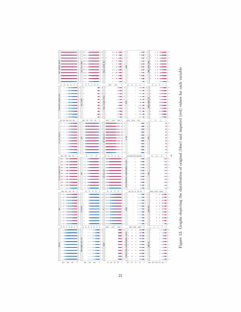
Figu
re12
:G
raph
sde
pict
ing
the
dist
ribu
tion
ofor
igin
al(b
lue)
and
impu
ted
(red
)va
lues
for
each
vari
able
21

Figu
re13
:H
isto
gram
sof
orig
inal
(blu
e)an
dim
pute
d(r
ed)
valu
es
22

Figure 14: Bivariate graphs of original and imputed values
23

Figure 15: Oil and gas recovery efficiency prediction performance using standardmultilinear regression using six variables
modeling. A standard case of multilinear regression here will serve to illustratethe shortcoming of the traditional approach, and as a benchmark for otheranalytic techniques.
Six variables frequently used in reservoir engineering were chosen to createa linear regression model that predicts the ultimate recovery efficiency. Thevariables are initial reservoir pressure, porosity, depth, oil and gas well spacing,and water saturation. The well spacing variables were log-transformed becausethey had broad ranges and their univariate distributions were approximatelylognormal.
Using a training set, standard linear regression was conducted to find thecoefficients that yield the most accurate estimate of oil and gas recovery efficien-cies. Testing results for predicting oil and gas recovery efficiencies are providedin Figure 15.
From the scatter plots in Figure 15 the multilinear regression’s performanceis poor; the predicted values of recovery efficiencies given in the y-axes show littlecorrelation with the actual data set recovery efficiency values in the x-axes. Forgas recovery efficiencies, the estimated values on the horizontal axis show widerscatter than the actual target values from the data set, shown on the verticalaxis. The inaccurate estimation may be because none of the individual inputvariables displayed bivariate correlation with oil or gas recovery efficiencies.
To examine whether any subset of input variables adopted above yield better
24

Figure 16: Frequency of variables selected as the best performing multilinearregression model
performance, we conducted another experiment. We created regression modelsusing all possible subset combinations of the six chosen variables and tested themodels. Then we selected the best performing model according to whicheverhad the smallest mean squared error. Because each training and testing of modeldrew from different randomized training and testing data sets, the process wasrepeated 100 times. Figure 16 shows that variables 1-4 were selected as thehighest performing linear regression model for the oil recovery prediction andthat the same variables plus variable 6 were selected for gas recovery. In order,variables 1-6 represent: initial reservoir pressure, average porosity, depth, oilwell spacing, gas well spacing, and average water saturation.
For oil recovery efficiency model, the first four variables were implemented.These variables were: 1. Initial reservoir pressure, 2. Average porosity, 3.Subsurface depth, and 4. Oil well spacing. For the gas recovery efficiencymodel, the selected variables were identical to the oil model, with the additionof 5. Average water saturation.
Multilinear regression models created with the selected variables were tested,and the results are provided in Figure 17.
The figures reveal that the performance show little improvement from theinitial case; the estimations are as scattered as in Figure 15.
Initially, the scope of analysis was limited to six input variables, which weredetermined by what we believed to have a direct influence on recovery efficienciesbased on engineering principles. However, it may be that correlations withrecovery efficiencies exist outside the span of the proposed six variables, or notat all. Because the database has many features (250+) for each reservoir entry,
25

Figure 17: Oil and gas recovery efficiency prediction performance of multilinearregression models with brute-force method to select variables
creating linear regression models with every possible combination of variablesis costly in time and computation. Sequential feature selection, proposed in thenext section, is an elegant alternative to this brute-force approach.
4.2 Multilinear Regression with Sequential Feature Selec-tion
Also known as feature subset selection, sequential feature selection selectsonly the variables that are relevant to the analysis, effectively reducing the di-mensions considered for a goal. This method is different from the previoussection in that, whereas the previous method required the modeler to selectthe variables, the algorithm selects the variables according to the intervariaterelationships present in the data set. Sequential feature selection is effectivewhen creating models with high dimensional data, which is common in machinelearning (Fisher and Lenz, 2007). Of different variations of the selection meth-ods, we have employed the sequential forward selection method as described inthe literature review section. After implementing the sequential forward featureselection method separately for oil and gas recovery factors, two groups of vari-ables from the dataset were produced. The selected variables are summarizedin Table 1.
Figure 18 shows the testing result: the estimated recovery efficiency is in they-axis, whereas the actual data set values are given in the x-axis. The estimation
26

Selected Variables Oil RF Selected Variables Gas RFAPI GRAVITY API GRAVITYAVERAGE ANNUAL SURFACE T DEPTHFRACTURE PRESSURE ELEVATIONGAS SPECIFIC GRAVITY FLUID CONTACTMID RESERVOIR DEPTH FRACTURE PRESSUREPORE VOLUME COMPRESSIBILITY FORMATION VOLUME FACTORPOROSITY PORE VOLUME COMPRESSIBILITYPRODUCTION POROSITYSTRATIGRAPHIC COMPARTMENT COUNT PRESSURETEMPERATURE DEPTH PRESSURE DEPTHTEMPERATURE GRADIENT PRODUCTIONTOTAL ORGANIC CONTENT STRATIGRAPHIC COMPARTMENT COUNTVISCOSITY TEMPERATURE STRUCTURAL COMPARTMENT COUNTWATER SATURATION TEMPERATUREWELL COUNT TEMPERATURE DEPTHWELL SPACING TEMPERATURE GRADIENT
THICKNESSTOTAL ORGANIC CONTENTWATER SALINITYWATER SATURATIONWELL COUNTWELL SPACING
Table 1: Variables selected after sequential feature selection
Figure 18: Oil and gas recovery efficiency prediction performance of linear re-gression models with sequentially selected variables
27

Figure 19: Frequency of variables selected after 1000 runs of sequential featureselection
accuracies significantly improved from Figure 15 and 17 though there are stillissues.
Because of the stochastic nature of separating training and testing datasets, resulting combinations of selected features may differ. To account for thiseffect, we have run 1000 cases of sequential feature selection, each with differenttraining and testing data sets randomly drawn from the same original data set.Figure 19 shows the number of times each variable was selected for the finalmodel after sequential variable selection. For concise representation, variablenames in the x-axes were replaced by corresponding variable IDs unique to eachvariable.
The frequency of selection varies greatly for each variable. To create andtest the final model, we have adopted variables that were selected more than90% of the time. These variables are in Table 2. The horizontal axes (“Target”)represent the values from the original data set, while the vertical axes (“Output”)represent values estimated by the model. The predictive accuracies are notas high as for the single sequential variable selection case but very close. Itis a significant improvement from the original multilinear regression model inFigures 15 and 17.
4.3 Conclusions and Discussions for Chapter 4
In this chapter, multilinear regression was used in three different ways. First,a multilinear regression model was created by selecting six variables from thedatabase that we believed to have the greatest influence on recovery factor.The model performed poorly, showing little and scattered correlation between
28

RF Oil RF GasPOROSITY WATER DEPTHPORE VOLUME COMPRESSIBILITY DEPTHWATER SATURATION FLUID CONTACTTOTAL ORGANIC CONTENT STRATIGRAPHIC COMPARTMENT COUNTWELL COUNT THICKNESSAPI GRAVITY POROSITYGAS SPECIFIC GRAVITY PORE VOLUME COMPRESSIBILITYTEMPERATURE DEPTH WATER SATURATIONTEMPERATURE GRADIENT WELL COUNTFRACTURE PRESSURE API GRAVITYWELL SPACING TEMPERATURE
TEMPERATURE GRADIENTFRACTURE PRESSUREPRESSUREPRESSURE DEPTHWATER SALINITY
Table 2: Variables selected after 1000 runs of sequential variable selection
Figure 20: Oil and gas recovery efficiency prediction performance for variablesselected after 1000 runs of sequential variable selection
29

the predicted values and the target values. Next, multilinear regression modelswere created using the variables that were selected from the forward sequentialvariable selection method. The model created with this method performed best,with strong positive trend between predicted and target recovery factor values.Finally, we repeated the sequential variable selection a 1000 times, and createda multilinear regression model using only the variables that were selected morethan 90% of the time. The final model created performed similarly to the modelcreated with a single run of sequential variable selection. In this chapter, wehave demonstrated that the recovery factors can be predicted to a certain degreeby using multilinear regression and a certain type of feature selection procedure.
5 Bayesian Network
Another model implemented is the Bayesian network model. Bayesian net-work is a probabilistic graphical model that represents a set of random variablesand their conditional dependencies. Bayes’ theorem for a bivariate conditionalrelationship is represented in the following equation.
P (A|B) =P (B|A)P (A)
P (B)
The theorem is used as an approach to systematically update a prior beliefgiven an evidence. As a simple example, generally we understand that thedeeper the reservoir, the higher the reservoir pressure. With that knowledge,if we were given a reservoir that is very deep, we would expect the pressureto be high accordingly. Bayes’ theorem provides a methodical way in whichthe expectations are handled with new information. Bayes’ theorem can begeneralized to include multiple variables simultaneously.
In a Bayesian network, a random variable is represented as a node, and aconditional dependency is represented as an edge. These components are usedtogether to represent a successive and/or simultaneous application of Bayes’theorem, which is used to systematically update prior probability distributionswhen new observations are made (Pearl, 2009). The network is able to take inmultiple variable observations, and accordingly update the estimated probabil-ities in related nodes. This approach draws from principles from graph theory,probability theory, machine learning (computer science), and statistics (Bishop,2006).
The Bayesian network has a few distinct advantages in achieving the goal
30

Figure 21: Bayesian network to estimate oil and gas recovery factors
of predicting recovery efficiency. 1) It is able to incorporate both the data andthe relationships between reservoir properties. 2) It can easily visualize variableinterdependencies, which can be difficult in other multidimensional models. 3)It can handle both continuous and categorical variables, which were neglected inthe previous stages. 4) It does not require a physical model. 5) The estimationsare quick because of its low computational cost.
5.1 Simple Naïve Bayesian Network Model
To predict oil and gas recovery efficiencies, we created and tested a naïve(meaning no relationship between inputs) Bayesian network. Figure 21 is asnapshot the network. 70% of the data were randomly selected to train themodel, while the remaining 30% were used to test the predictive performanceof the network.
To allow numeric computation of conditional probabilities, continuous vari-ables were discretized into three or four segments. Again, oil and gas well spacingvariables were log-transformed. Because each node shows the probability distri-bution of the variable rather than a specific value, the numeric estimate of oiland gas recovery efficiencies were estimated by calculating the expected valueof the discretized probability distribution. The testing results are in Figure 22.
The agreement with the actual values is similar to that of simple linear re-gression. A difference is in that the predicted values of recovery efficienciesshow slight striations. These striations are artifacts of discretization of continu-ous variables, which compartmentalized the multidimensional space and placed
31

Figure 22: Oil and gas recovery efficiency prediction performance for Bayesiannetwork
the data in its segments. Increasing the number of discretization for each vari-able will make the prediction striations smoother; however, the likelihood of adata point’s presence in each discretized segment quickly decreases. With thescale of our current database, three or four discrete segments per variable areappropriate.
5.2 Engineering Variables vs. Geology Variables
During the course of our research, one of the questions that surfaced was: be-tween engineering and geology variables, which is a better predictor of recoveryfactors? In the literature, there are a few authors who assert that geologi-cal factors have major impact on the hydrocarbon recovery. For instance, thewidely-cited Tyler and Finley (1992) claimed that there is a “well-defined rela-tion between reservoir architecture and conventional (primary and secondary)recovery efficiency.” To determine whether the claim is true, we designed anexperiment where two naïve Bayesian network models are made, one with onlyengineering variables, and the other from only geology variables. We train andtest the same way to determine which of the two models yield better predic-tive results, and thus conclude which group of variables are better predictors ofrecovery factor in general.
First, the engineering naïve Bayesian network model is given in Figure 23.The variables selected were variables commonly used in reservoir engineering:
32

Figure 23: Naive Bayesian network with engineering variables
Model / Variable Mean of Error (%) StDev. of ErrorGeology / RF Oil 0.785 14.765Geology / RF Gas 1.635 12.636
Engineering / RF Oil 0.107 12.788Engineering / RF Gas 1.265 12.057
Table 3: Summary of performance for engineering and geology BN models
initial pressure, initial temperature, initial water saturation, depth, porosity,and well spacing. After training the model, it was tested against actual datasets.The results of testing is given in Figure 24.
Next, the geology model was constructed as in Figure 25. The geologi-cal model involves the following categorical variables: structural setting, Ballydepositional environment category, depositional system, and current tectonicregime. The testing performance of the geological model is given in Figure 26.
The scattergraphs on Figures 24 and 26 show striations that we attributeto the discrete nature of analysis. The histograms in both figures are showingvalues of error, which is calculated as the difference between actual and predictedrecovery factor values. Both models perform similarly in estimating the recoveryfactors of reservoirs; Table 3 summarizes the capability of both models in theform of mean and standard deviation of error. The two aspects is also explainedusing the terms bias and precision, respectively. We have concluded that there
33

Figure 24: Performance of naive Bayesian network with engineering variables
Figure 25: Naive Bayesian network with geology variables
34

Figure 26: Performance of naïve Bayesian network with geology variables
35

is marginal difference in predictability in geologic and engineering variables.
5.3 Experiments Using Bayesian Network
Two experiments were performed to determine the robustness of Bayesiannetwork models. In section 5.3.1, a number of comparative tests are performedto demonstrate what the effect of discretization of continuous variables are onthe prediction of a dependent variable. In section 5.3.2, noise in a bivariate cor-relation is introduced progressively to see how it affects the estimation outcomeof a dependent variable. Finally, in section 5.3.3, we see how the inclusion of anunrelated node affects the predictive outcome.
5.3.1 Effect of Discretization in Prediction
Bayesian analysis requires continuous variables to be discretized into seg-ments so that Bayes’ theorem could be applied. This section of the reportexamines how different sizes of discretization applied to the variables affect thepredictive outcome of the model.
To observe the effect, we have selected two variables from the databasethat show relatively strong bivariate correlation: average oil formation thick-ness (OTHK) in feet, and the original oil in place (OIP) in barrels. Both vari-ables were log-transformed to make approximately normal distributions. Thevariables are represented as histograms, and the relationship is visualized as ascattergram in Figure 28. Each variable is discretized in three, five, and ninesegments, and average oil formation thickness is used as the input value to es-timate original oil in place. A graphical model of the simple Bayesian networkis provided in Figure 27.
The two-variable system is discretized in three, five, and nine different num-bers of discretized segments, and is tested in a similar to the previous sections.The results are presented in Figure 29.
From Figure 29, we can first see that the number of striations in the outputaxis (y-axis) of the scatter graph coincides with the number of discretizationapplied to the output variable, and that the spread of target values is centeredaround the y = x line, which represent a perfect estimation. The striationsindicate that the values the model can predict is limited to a set number. As thenumber of discretization increases, the spread in the predicted values increase;however it does not seem to improve the accuracy significantly, as shown in thehistograms in Figure 29.
It is also important to note that increasing the number of discretization
36

Figure 27: A simple example Bayesian network
increases the number of segments in data space, often in high-order dimensions.Therefore it is imperative that the discretization is large enough so that thereare enough data points in each section of the segmented data space to make itstatistically representative; otherwise the model will either not have data for itto train or be biased, rendering it less effective.
5.3.2 Effect of Noise in Correlations
Another aspect that may interfere with an accurate estimation of dependentvariable is the noise in intervariate correlations. In this test we introduce anincreasing amount of noise to a perfect correlation, create Bayesian networkmodels with each variable combination and see how they perform. Unlike theprevious section, we have created synthetic data to test for the effect of noise inpredictions.
Four independent variables were generated using different ranges of uniformdistribution. A dependent variable (labelled E in Figure 30) is a linear combi-nation of the remaining variables, A, B, C, and D. Variable E was generatedusing the following equation. Histograms showing the univariate distributionis provided in Figure 31, and the bivariate relationships with E is shown inscattergraphs in Figure 32.
E = 2A+ 3B � 4C + 5D + ✏
37

Figure 28: Variables used to examine the effects of discretization in Bayesiannetwork
38

Figure 29: Simple Bayesian network model with varying number of discretiza-tion of the output variable
39

Figure 30: Bayesian network for synthetic data
In the above equation, E is a linear combination of variables A, B, C and D,with arbitrary coefficients assigned for each input variable. The last term in theequation ✏ represents the error, or the noise term. Three different noise wereused: no noise, 50% noise and 200% noise. Here, 50% error represents a randomvalue picked from a uniform distribution, whose range corresponds to 50% ofthe range of variable E, and with the same expected value as variable E. 70%of the data were randomly selected to train the Bayesian network models, whilethe remaining 30% were used to test by comparing with the actual values fromthe dataset. The results of training and testing with different levels of noise areprovided in Figure 33.
An observation of the plots in Figure 33 reveals that the naïve Bayesiannetwork model is susceptible to noise in data. The case with zero noise fallsclosely in line with the line of perfect estimation (y = m), while there are somedeviations due to the effect of discretization. However, when 50% and 200%noise is added to the data, the estimations are heavily affected. The standarddeviation of histograms of error for the two cases are 13.01 and 34.84, which aresignificantly higher than that of no error (2.88). The plots in Figure 33 showthat the Bayesian network is not robust against noise in the data.
5.3.3 Effect of Unrelated Node in a Bayesian Network
The final source of error to be discussed in this report is the inclusion of anunrelated node in the design of a Bayesian network. Because Bayesian networkis often designed by the users, it is possible that a variable that has no relationto the dependent variable is added to a model that is otherwise sound. To seehow a variable of no correlation affects the prediction, the following test wasconducted.
Taking the same set of variables and data as in section 5.3.2, we added
40
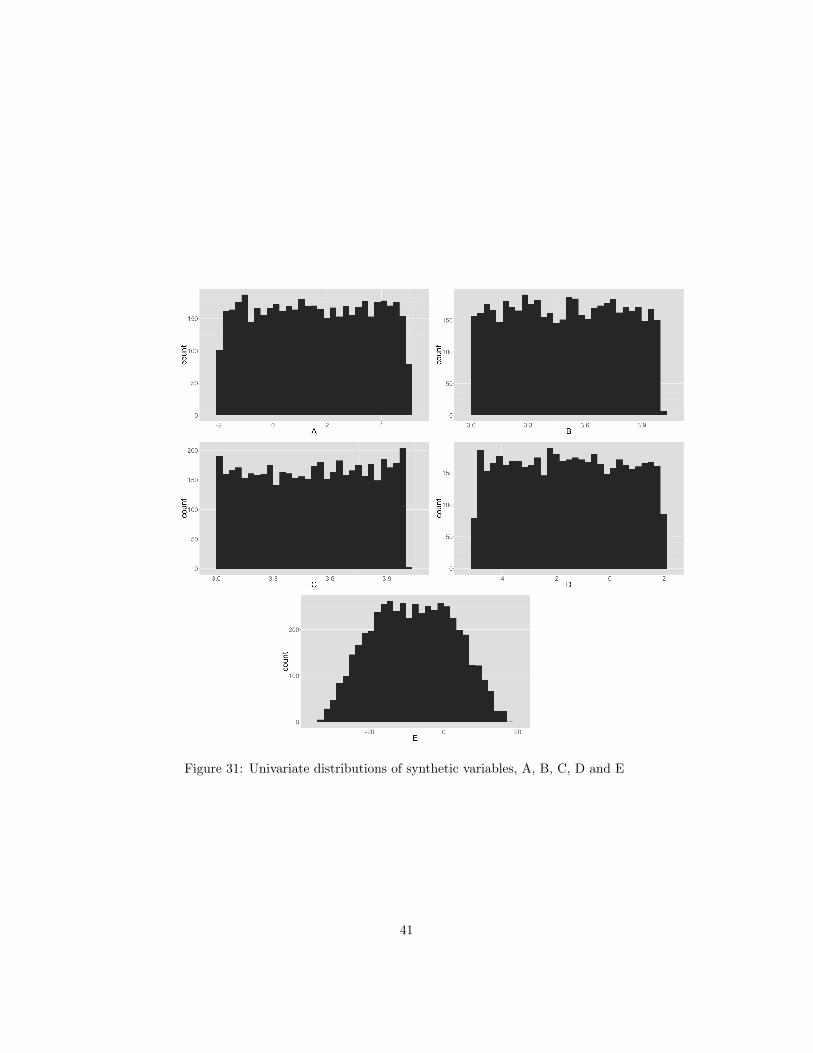
Figure 31: Univariate distributions of synthetic variables, A, B, C, D and E
41
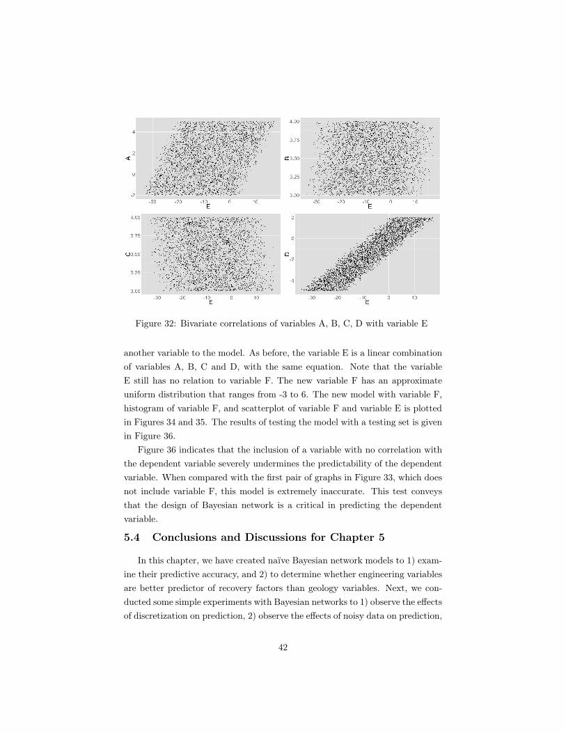
Figure 32: Bivariate correlations of variables A, B, C, D with variable E
another variable to the model. As before, the variable E is a linear combinationof variables A, B, C and D, with the same equation. Note that the variableE still has no relation to variable F. The new variable F has an approximateuniform distribution that ranges from -3 to 6. The new model with variable F,histogram of variable F, and scatterplot of variable F and variable E is plottedin Figures 34 and 35. The results of testing the model with a testing set is givenin Figure 36.
Figure 36 indicates that the inclusion of a variable with no correlation withthe dependent variable severely undermines the predictability of the dependentvariable. When compared with the first pair of graphs in Figure 33, which doesnot include variable F, this model is extremely inaccurate. This test conveysthat the design of Bayesian network is a critical in predicting the dependentvariable.
5.4 Conclusions and Discussions for Chapter 5
In this chapter, we have created naïve Bayesian network models to 1) exam-ine their predictive accuracy, and 2) to determine whether engineering variablesare better predictor of recovery factors than geology variables. Next, we con-ducted some simple experiments with Bayesian networks to 1) observe the effectsof discretization on prediction, 2) observe the effects of noisy data on prediction,
42
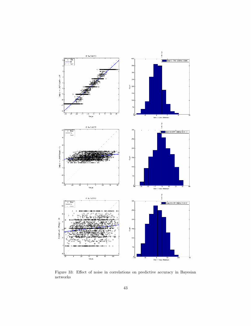
Figure 33: Effect of noise in correlations on predictive accuracy in Bayesiannetworks
43

Figure 34: Bayesian network model with an unrelated node, represented asvariable F
Figure 35: Histogram of variable F and scatterplot of variable F and E
Figure 36: Testing Bayesian network with an unrelated node
44

and 3) examine how an introduction of an unrelated variables affects prediction.On the first part of this chapter, we have concluded that the naïve Bayesian
networks perform at a similar level as the multilinear regression model createdin section 4.1. The results also suggest that the two naïve Bayesian networkscreated with only engineering variables and only geology variables perform sim-ilarly in predicting the recovery factors. Finally, we have demonstrated thatnoise in data and the inclusion of an uncorrelated variable both have detri-mental effect on the predictive power of the Bayesian network models, whichserves as evidence against the robustness of the model. The test on the extentof discretization has exemplified the limitation of this model—that it requirescontinuous variables to be discretized for the Bayesian network to be applicableat all.
There are many aspects of this chapter that can be explored further. It is im-portant to analyze how other possible permutations of the model influences thepredictability of recovery factors. It will also be worthwhile to know how differ-ent selection of variables can improve or deteriorate the predictive performanceof the model.
6 Analog Recommender System
Another way in which the dataset can be useful is through a reservoir ana-log recommender system. In exploration and production, analog reservoirs arevaluable because they help suggest production methods and optimize plans forsimilar and/or nearby wells. Reservoir analogs can be useful in situations wherelow seismic resolutions fail to provide detailed information about the forma-tion at hand. This portion of the report discusses how an analog recommendersystem was created with the concept of similarity ranking.
In this research, distance-based similarity measure is the core method em-ployed to create recommender systems. The analysis assumes that distance indata space is inversely proportional to similarity, and different distance mea-sures provide ways to quantify and compare the proximity. In this section ofthe report, we employ different various distance measures with and withoutprincipal component analysis (PCA) to examine how the final lists ranked bydistance vary. The distance measures used are Euclidean distance, Manhattandistance, and Minkowski distance. The chapter will conclude by discussing thevarious aspects of each distance measures, and how the introduction of PCAaffects the analysis.
45

6.1 Similarity Ranking with Euclidean Distance
For the distance measure method to be valid, the data type must be nu-meric; other variable types cannot be used to calculate Euclidean distance. Anyvariables that are non-numeric (e.g. string variables and categorical variables)were discarded to create a dataset that only contains quantitative variables.Subsequently, the dataset went through a pre-processing stage that involvestransforming each variable to approximate normal distributions using Box-Coxtransformations (Box and Cox, 1964). After the transformations, all variableshad distributions that closely resemble a normal distribution with mean centeredaround zero and a standard deviation of 1. The distributions of two variablesbefore and after transformations are given in Figure 37. The variables thatwent through a log transformations are: injection and production well counts,structural compartment count, dip, area, oil column height, hydrocarbon col-umn height, stratigraphic compartment count, gross average thickness, net paythickness, permeability, OOIP, OGIP, cumulative oil and gas production, vis-cosity, formation volume factor, and temperature.
Normalizing the variables is necessary in order to make the distance measures(and thus similarity measures) scale-invariant. Take for instance, a trivariatesystem that contains porosity, permeability and depth. Determining similarityby calculating Euclidean distances with variables that are not transformed willplace undue weight on the porosity variable, because in general porosity vari-ables are much closer numerically compared to permeability or depth. Thereforewe propose transforming all variables to normal distribution in order to elimi-nate the effect of scale inconsistency.
After the variables were transformed to approximate normal distributions,we have calculated the distance between each reservoir entries in the database.This is easily represented as a triangular matrix that contains the distancevalue for each pair of reservoir entries. Because the matrix size is so large(n⇥ n matrix, where n is the number of entries), presentation of the matrix isomitted. However, we can now select a reservoir from the dataset and rank otherreservoirs according to similarity, or distance. The top few reservoir instanceswith the lowest distance will serve as recommendations for reservoir analogs.
As an example, we have selected an entry with the name “ANETH [PARA-DOX (DESERT CREEK)] CF24 [CR24]” and ranked other entries by lowestEuclidean distance. Table 4 lists the top 10 entries given by the method usedin this section. Intuitively, the entry with the smallest distance with the given
46

Figure 37: OOIP and Area variables before and after Box-Cox transformations
47

Rank Entry Name Distance1 ANETH [PARADOX (DESERT CREEK)] CF24 [CR24] 0.00002 JUDY CREEK [SWAN HILLS (JUDY CREEK A POOL)] CF139 [CR139] 2.67753 NORTH BURBANK [BURBANK (RED FORK)] SF528 [SR528] 2.77974 NIPISI [WATT MOUNTAIN (GILWOOD A POOL)] SF526 [SR526] 2.79315 SLAUGHTER [SAN ANDRES] CF290 [CR290] 2.82716 VACUUM [SAN ANDRES] CF319 [CR319] 2.91907 MITSUE [WATT MOUNTAIN (GILWOOD A)] SF504 [SR504] 2.92528 PENWELL [SAN ANDRES] CF241 [CR241] 2.93129 EL BORMA [KIRCHAOU] SF243 [SR243] 3.081410 RAGUBA [WAHA] SF626 [SR626] 3.1547
Table 4: Top 10 most similar reservoirs given by Euclidean distance
reservoir is the given entry itself, which has a Euclidean distance of zero. Table 5provides some information about the reservoirs ranked top 10.
6.2 Similarity Ranking with Euclidean Distance and Prin-cipal Component Analysis
In this section, we take a similar approach as the previous section whileintroducing principal component analysis (PCA). In other words, instead ofcalculating the Euclidean distance between data points in normalized data space,we calculate the Euclidean distance in a normalized space constructed withprincipal components taken from the data.
With the 30 numeric variables from the original data, we have applied PCA.The analysis rotates the principal axes of the 30-dimensional space while main-taining the orthogonal basis between axes in order to align the axes so that itcaptures the variability of the data, or equivalently, maximizes the covariancematrix both in trace and determinant (Venables and Ripley, 1999). Once therotation optimization process is complete, the new rotated axes are called prin-cipal components. The rotation matrix is given in two parts in Tables 6 and7. After the rotation is complete, the original data is projected to the princi-pal components. The first 10 entries of the data transformed into the principalcomponents is shown in Table 8. A summary of principal components is givenin Table 9. The variances of the first 10 principal components is provided inFigure 38. Note that the principal components are labeled by the order of stan-dard deviation or variance it contains of the data used. In Table 9, it is apparentthat the first 22 principal components are required to contain about 95% of thevariance in the data. Principal components 23 through 30 captures only 5%of the overall variance, and therefore it will be discarded. The rejection has
48

RA
NK
12
34
56
78
910
WELL_
CO
UN
T_
PR
OD
500
170
8910
130
2362
700
164
148
82W
ELL_
CO
UN
T_
INJ
500
27
3840
62
4840
228
STR
UC
T_
CO
MP
RT
_C
OU
NT
11
11
11
11
11
DEP
TH
1676
.426
03.0
883.
916
79.5
1554
.512
95.4
1737
.499
0.6
2398
.815
45.3
DIP
2.0
0.5
1.5
0.5
0.5
2.2
0.5
2.0
0.5
2.5
AR
EA
195.
312
9.5
91.0
386.
740
4.7
29.4
566.
640
.116
1.9
25.1
HC
_C
OL_
HEIG
HT
_O
IL79
.370
.167
.138
.112
1.9
137.
265
.512
1.9
91.4
137.
8H
C_
CO
L_
HEIG
HT
79.3
70.1
67.1
38.1
121.
913
7.2
93.0
121.
910
0.6
214.
0ST
RA
TI_
CO
MP
RT
_C
OU
NT
35
34
44
32
49
TH
ICK
NESS
_G
RO
SS_
AV
G54
.86
70.1
030
.48
30.4
827
4.32
112.
7824
.38
121.
9210
7.59
70.1
0N
ET
_G
RO
SS_
RA
TIO
0.45
0.39
0.70
0.30
0.49
0.40
0.40
0.49
0.50
0.36
TH
ICK
NESS
_N
ET
_PA
Y15
.24
18.2
915
.24
4.27
21.3
445
.72
3.96
35.9
730
.48
25.2
4P
OR
OSI
TY
109
1714
1212
1311
1717
K_
AIR
1545
5025
010
1723
03
500
200
SW23
1630
3120
1636
3520
18O
OIP
175.
0113
0.14
106.
7613
1.73
446.
4399
.09
141.
7652
.34
226.
7229
8.31
OG
IP0.
131
0.05
30.
045
0.04
30.
379
0.01
00.
039
0.06
80.
020
0.03
6C
UM
_O
IL70
.64
50.1
223
.86
56.3
220
0.15
36.5
960
.78
16.5
511
1.37
108.
66C
UM
_G
AS
0.01
100.
0187
0.01
070.
0092
0.02
820.
0152
0.02
680.
0133
0.02
030.
0185
AP
I41
4139
4130
3841
3942
43V
ISC
0.53
1.28
3.00
0.89
2.00
0.96
0.60
2.66
0.29
3.56
VIS
C_
TEM
P50
8949
4942
6660
5882
38G
AS_
SPEC
_G
RAV
0.75
00.
763
0.86
60.
850
0.90
10.
700
0.76
40.
733
0.71
90.
764
FV
F1.
350
1.40
81.
200
1.20
01.
228
1.28
81.
447
1.24
01.
700
1.58
0T
EM
P37
9434
4726
2257
2161
49P
_I
1498
5.51
2417
0.18
8286
.92
1803
0.96
1180
8.86
1124
2.59
1809
3.11
1277
5.67
2603
4.74
1639
4.29
RF_
OIL
_U
LT53
.046
.048
.044
.045
.031
.346
.040
.059
.043
.2R
F_
GA
S_U
LT76
.17
76.3
374
.33
75.6
780
.33
69.0
073
.17
77.1
783
.33
79.6
7W
ELL_
SPA
C_
OIL
0.12
10.
324
0.04
00.
648
0.06
90.
081
1.29
50.
040
0.44
50.
184
WELL_
SPA
C_
GA
S0.
8072
0.74
700.
6578
0.68
800.
9985
0.72
520.
4858
0.50
470.
7757
0.83
63
Tabl
e5:
Info
rmat
ion
onth
ere
serv
oirs
rank
edto
p10
byE
uclid
ean
dist
ance
49

Figure 38: Variance of the first 10 principal components
reduced the number of dimensions from 30 to 22 while maintaining most of thebehavior of data in the original data set. This is the main idea of dimensionreduction through PCA.
To continue with implementing similarity ranking, we create the distancematrix using Euclidean distance and the 22-dimensional data retrieved fromPCA. Using the same entry “ANETH [PARADOX (DESERT CREEK)] CF24[CR24],” we have sorted the reservoirs according to distance. The top 10 rankedresults are provided in Table 10. The data for these entries are presented inTable 10. We can see that there are a few overlaps between the results fromthis section and the previous section, but the distance values are different.
6.3 Similarity Ranking with Manhattan Distance
Manhattan distance can also be used to quantify the extent of dissimilarity.Manhattan distance is absolute difference of the cartesian coordinates. Mathe-matically expressed, the distance measure is as follows.
50

PC
1P
C2
PC
3P
C4
PC
5P
C6
PC
7P
C8
PC
9P
C10
PC
11P
C12
PC
13P
C14
PC
15W
ELL_
CO
UN
T_
PR
OD
0.32
7-0
.031
0.14
4-0
.082
0.10
4-0
.083
0.05
7-0
.193
0.02
40.
154
-0.0
55-0
.048
-0.0
34-0
.080
0.28
7W
ELL_
CO
UN
T_
INJ
0.30
8-0
.071
0.10
4-0
.080
0.02
8-0
.082
0.16
1-0
.239
-0.0
300.
156
0.03
30.
053
0.02
30.
104
0.31
6ST
RU
CT
_C
OM
PR
T_
CO
UN
T0.
094
-0.1
14-0
.148
0.14
1-0
.078
-0.2
230.
250
-0.4
130.
175
-0.0
320.
145
-0.2
61-0
.349
-0.4
930.
116
DEP
TH
-0.2
99-0
.207
0.13
7-0
.119
-0.1
660.
058
0.16
1-0
.132
0.02
30.
099
-0.2
040.
136
0.05
80.
044
0.21
1D
IP-0
.057
-0.2
54-0
.298
0.15
20.
173
0.22
60.
106
0.00
2-0
.040
0.04
90.
152
0.02
5-0
.186
0.08
9-0
.074
AR
EA
0.23
6-0
.098
0.34
7-0
.132
-0.0
70-0
.076
-0.1
450.
038
-0.1
53-0
.133
-0.1
36-0
.207
-0.0
13-0
.031
-0.1
11H
C_
CO
L_
HEIG
HT
_O
IL0.
107
-0.3
34-0
.052
0.16
70.
118
0.29
70.
094
-0.2
95-0
.153
-0.1
310.
037
0.12
10.
123
0.11
3-0
.134
HC
_C
OL_
HEIG
HT
0.10
5-0
.379
-0.0
500.
171
0.19
30.
175
0.09
2-0
.096
-0.1
22-0
.197
0.03
50.
003
0.06
30.
087
-0.1
27ST
RA
TI_
CO
MP
RT
_C
OU
NT
0.11
2-0
.175
-0.1
540.
121
-0.0
52-0
.393
-0.1
52-0
.012
0.32
90.
014
-0.0
500.
000
0.33
30.
225
0.03
6T
HIC
KN
ESS
_G
RO
SS_
AV
G0.
064
-0.3
06-0
.133
0.27
2-0
.067
-0.1
98-0
.239
0.21
30.
174
0.08
3-0
.025
0.06
60.
057
-0.1
080.
080
NET
_G
RO
SS_
RA
TIO
-0.0
82-0
.017
-0.2
28-0
.355
-0.0
110.
267
0.03
60.
188
-0.2
030.
274
0.23
7-0
.136
-0.1
06-0
.134
0.12
0T
HIC
KN
ESS
_N
ET
_PA
Y0.
017
-0.3
35-0
.216
0.09
6-0
.100
0.01
3-0
.198
0.37
10.
014
0.22
70.
099
-0.0
290.
002
-0.1
730.
136
PO
RO
SIT
Y0.
161
0.09
7-0
.368
-0.1
38-0
.235
-0.1
970.
163
0.02
3-0
.067
-0.1
540.
028
-0.0
32-0
.023
0.17
4-0
.158
K_
AIR
0.07
90.
084
-0.3
74-0
.237
-0.2
21-0
.046
0.14
1-0
.107
0.15
8-0
.083
-0.0
32-0
.098
0.13
20.
144
-0.1
96SW
0.05
50.
077
0.19
10.
232
0.03
9-0
.284
0.19
7-0
.005
-0.1
220.
352
0.41
60.
185
-0.1
750.
402
-0.2
14O
OIP
0.26
4-0
.222
0.10
0-0
.171
-0.1
650.
012
-0.1
750.
008
-0.2
82-0
.022
-0.0
54-0
.165
-0.0
100.
088
-0.0
92O
GIP
0.23
2-0
.171
0.16
3-0
.195
0.02
10.
046
0.17
60.
221
0.21
60.
156
-0.0
380.
224
-0.0
890.
001
-0.0
90C
UM
_O
IL0.
195
-0.2
05-0
.041
-0.3
07-0
.045
-0.0
52-0
.293
-0.1
21-0
.180
0.05
50.
060
-0.1
16-0
.035
0.11
1-0
.008
CU
M_
GA
S0.
177
-0.1
140.
081
-0.2
870.
057
-0.0
430.
045
0.14
50.
256
-0.1
280.
009
0.50
7-0
.282
-0.2
30-0
.251
AP
I-0
.227
-0.1
060.
142
-0.1
190.
340
-0.3
04-0
.041
0.10
8-0
.108
0.02
70.
170
-0.1
050.
010
-0.0
260.
122
VIS
C0.
264
0.05
9-0
.033
0.05
7-0
.146
0.24
00.
308
0.25
30.
096
-0.0
23-0
.092
0.02
00.
067
0.02
60.
150
VIS
C_
TEM
P-0
.236
-0.2
010.
007
-0.0
81-0
.084
-0.2
330.
005
-0.0
97-0
.166
0.03
6-0
.018
-0.0
01-0
.029
-0.2
26-0
.443
GA
S_SP
EC
_G
RAV
-0.0
170.
048
0.09
5-0
.106
0.09
10.
342
-0.3
66-0
.334
0.51
70.
278
0.14
3-0
.096
0.08
60.
023
-0.2
32FV
F-0
.157
-0.1
730.
109
-0.0
490.
046
0.00
20.
109
0.17
30.
311
-0.0
89-0
.167
-0.4
79-0
.491
0.39
2-0
.056
TEM
P-0
.292
-0.1
510.
081
-0.1
69-0
.238
-0.0
970.
086
-0.1
54-0
.019
0.02
2-0
.076
0.18
60.
096
-0.0
54-0
.056
P_
I-0
.252
-0.2
870.
077
-0.0
39-0
.196
0.04
40.
145
-0.0
810.
046
0.04
8-0
.213
0.09
50.
001
0.17
60.
216
RF_
OIL
_U
LT-0
.089
-0.0
31-0
.280
-0.3
790.
224
-0.1
170.
015
-0.1
150.
025
0.14
00.
107
0.11
50.
046
0.19
10.
179
RF_
GA
S_U
LT-0
.014
-0.0
07-0
.131
-0.1
520.
552
-0.1
16-0
.040
0.02
00.
044
-0.3
78-0
.159
0.09
10.
001
0.00
90.
106
WELL_
SPA
C_
OIL
-0.0
84-0
.060
0.15
7-0
.068
-0.3
060.
064
-0.1
68-0
.002
0.12
1-0
.528
0.61
70.
109
-0.0
650.
102
0.27
4W
ELL_
SPA
C_
GA
S-0
.020
-0.1
380.
204
-0.1
400.
124
-0.0
100.
421
0.18
50.
154
-0.0
370.
287
-0.3
260.
536
-0.1
60-0
.142
Tabl
e6:
PC
Aro
tati
onm
atri
x(1
/2)
51

PC
16P
C17
PC
18P
C19
PC
20P
C21
PC
22P
C23
PC
24P
C25
PC
26P
C27
PC
28P
C29
PC
30W
ELL_
CO
UN
T_
PR
OD
0.05
90.
062
-0.3
22-0
.019
-0.0
23-0
.019
0.20
90.
128
0.26
0-0
.228
-0.6
260.
009
0.04
3-0
.010
-0.0
09W
ELL_
CO
UN
T_
INJ
0.10
30.
320
-0.3
370.
126
0.17
3-0
.058
0.05
5-0
.067
-0.2
020.
301
0.48
2-0
.058
0.02
60.
013
0.02
2ST
RU
CT
_C
OM
PR
T_
CO
UN
T-0
.137
-0.1
580.
259
-0.0
53-0
.039
0.00
6-0
.150
-0.0
33-0
.012
0.00
80.
086
-0.0
210.
000
0.01
70.
018
DEP
TH
-0.1
11-0
.178
0.03
60.
051
-0.0
04-0
.169
0.04
90.
042
-0.0
51-0
.070
0.03
20.
029
-0.1
21-0
.052
-0.7
30D
IP0.
199
-0.0
94-0
.147
0.43
4-0
.375
-0.1
060.
071
0.18
10.
401
0.10
40.
145
0.08
50.
042
-0.0
46-0
.020
AR
EA
-0.0
61-0
.015
0.09
9-0
.289
-0.0
76-0
.173
0.09
00.
060
0.40
30.
037
0.31
40.
454
0.10
7-0
.144
-0.0
29H
C_
CO
L_
HEIG
HT
_O
IL-0
.076
0.12
90.
120
-0.1
690.
100
0.06
0-0
.021
-0.0
69-0
.112
-0.0
37-0
.124
-0.0
34-0
.108
-0.6
430.
075
HC
_C
OL_
HEIG
HT
0.06
30.
131
0.08
5-0
.260
0.06
9-0
.020
0.03
6-0
.085
-0.0
820.
084
-0.1
330.
118
0.08
30.
679
-0.1
50ST
RA
TI_
CO
MP
RT
_C
OU
NT
-0.3
020.
384
0.22
40.
098
-0.3
76-0
.027
-0.0
120.
139
0.00
7-0
.041
-0.0
12-0
.030
0.01
00.
011
-0.0
34T
HIC
KN
ESS
_G
RO
SS_
AV
G0.
176
-0.2
20-0
.198
-0.1
590.
183
0.05
50.
105
-0.0
240.
040
0.04
30.
064
0.12
1-0
.620
-0.0
020.
058
NET
_G
RO
SS_
RA
TIO
-0.3
710.
333
0.05
8-0
.122
-0.0
28-0
.174
0.04
30.
112
-0.0
270.
005
-0.0
360.
124
-0.3
600.
069
0.08
8T
HIC
KN
ESS
_N
ET
_PA
Y-0
.119
-0.0
37-0
.059
-0.0
820.
284
-0.0
620.
011
-0.0
31-0
.010
0.05
2-0
.025
-0.0
940.
615
-0.1
48-0
.097
PO
RO
SIT
Y-0
.115
0.00
8-0
.062
0.23
90.
180
-0.0
390.
120
-0.6
040.
138
0.00
0-0
.140
0.24
0-0
.031
-0.0
42-0
.131
K_
AIR
0.29
3-0
.123
-0.1
18-0
.298
0.06
5-0
.438
-0.1
170.
373
-0.1
000.
111
-0.0
67-0
.063
0.04
7-0
.052
0.01
7SW
-0.2
72-0
.253
-0.0
01-0
.140
0.08
6-0
.100
0.03
10.
135
-0.0
09-0
.020
-0.0
100.
014
0.00
60.
029
0.00
2O
OIP
-0.1
00-0
.193
0.04
90.
078
-0.0
90-0
.093
-0.0
87-0
.124
0.17
20.
028
0.02
9-0
.702
-0.1
620.
105
0.00
7O
GIP
0.12
40.
095
0.09
20.
120
0.09
40.
051
-0.7
25-0
.036
0.11
7-0
.051
-0.0
850.
131
-0.0
630.
010
-0.0
23C
UM
_O
IL0.
049
-0.3
100.
106
0.29
8-0
.063
0.26
20.
015
0.20
6-0
.474
-0.0
16-0
.085
0.32
20.
045
0.01
50.
031
CU
M_
GA
S0.
032
0.05
20.
156
0.01
2-0
.075
-0.1
140.
466
0.00
9-0
.144
-0.0
020.
029
-0.1
320.
016
-0.0
230.
018
AP
I0.
266
-0.0
230.
042
-0.1
08-0
.325
-0.3
21-0
.095
-0.3
69-0
.182
0.27
5-0
.205
0.01
5-0
.003
-0.1
570.
004
VIS
C-0
.198
-0.2
78-0
.230
-0.2
77-0
.521
0.21
1-0
.012
-0.1
49-0
.192
0.10
90.
023
0.04
10.
052
-0.0
220.
023
VIS
C_
TEM
P-0
.053
0.19
3-0
.552
-0.0
92-0
.188
0.14
6-0
.129
-0.0
22-0
.114
-0.3
080.
102
-0.0
110.
053
0.00
6-0
.036
GA
S_SP
EC
_G
RAV
-0.1
46-0
.128
-0.1
48-0
.029
-0.0
19-0
.111
0.00
5-0
.291
0.03
70.
075
0.01
90.
042
0.02
70.
057
-0.0
10FV
F0.
001
0.15
6-0
.063
-0.0
540.
106
0.19
40.
115
0.04
8-0
.080
0.06
5-0
.055
-0.0
88-0
.034
-0.0
94-0
.026
TEM
P-0
.150
-0.0
29-0
.029
-0.0
130.
048
0.28
40.
023
0.10
00.
240
0.65
3-0
.225
0.02
60.
037
0.03
90.
216
P_
I-0
.030
-0.1
340.
045
0.05
70.
008
-0.2
950.
044
-0.1
66-0
.032
-0.3
530.
067
0.09
10.
092
0.12
50.
582
RF_
OIL
_U
LT0.
193
-0.0
850.
154
-0.3
62-0
.026
0.42
50.
047
-0.1
030.
269
-0.2
150.
220
-0.1
030.
068
0.00
8-0
.035
RF_
GA
S_U
LT-0
.480
-0.2
49-0
.250
0.05
50.
170
-0.1
16-0
.168
0.11
70.
023
0.03
30.
061
-0.0
02-0
.009
0.00
40.
050
WELL_
SPA
C_
OIL
0.01
00.
056
-0.1
61-0
.031
-0.0
280.
017
-0.1
090.
043
0.05
7-0
.092
-0.0
21-0
.002
0.00
2-0
.001
-0.0
40W
ELL_
SPA
C_
GA
S0.
023
-0.1
240.
034
0.20
10.
152
0.08
40.
188
0.06
10.
021
-0.0
980.
062
-0.0
47-0
.030
-0.0
120.
044
Tabl
e7:
PC
Aro
tati
onm
atri
x(2
/2)
52

Dat
aEnt
ryP
C1
PC
2P
C3
PC
4P
C5
PC
6P
C7
PC
8P
C9
PC
10P
C11
PC
12P
C13
PC
14P
C15
1-1
.720
-4.9
20-0
.725
1.12
5-2
.265
2.11
1-0
.334
0.26
4-0
.251
1.31
8-0
.133
-0.0
060.
124
0.57
90.
982
2-2
.018
-3.7
670.
727
-0.2
06-1
.853
2.03
4-0
.530
0.80
90.
092
0.74
9-0
.160
-1.8
530.
326
0.06
4-0
.083
5-0
.373
-2.9
821.
052
-0.3
99-0
.230
1.78
7-0
.870
-0.7
80-1
.033
0.36
1-0
.459
0.11
5-0
.013
0.56
1-0
.291
61.
764
-2.4
520.
699
-2.6
75-0
.697
0.37
0-1
.012
-0.7
42-1
.314
0.35
60.
681
-0.3
53-0
.566
1.27
4-0
.915
7-0
.132
-1.2
781.
733
-0.3
420.
472
0.98
3-0
.741
0.59
0-1
.250
-0.4
830.
393
-0.3
06-0
.659
-0.0
98-0
.096
81.
856
-3.1
95-0
.217
-1.4
34-0
.028
0.26
4-1
.513
-1.2
25-0
.224
0.53
9-0
.622
-0.2
84-0
.525
0.73
4-0
.715
9-0
.482
-2.3
100.
457
1.17
4-1
.915
1.20
90.
598
-0.2
58-0
.965
0.10
1-0
.634
-0.3
38-0
.509
-0.5
62-0
.981
100.
143
-4.0
480.
117
1.14
1-1
.200
0.41
7-0
.747
-0.8
64-0
.921
0.21
5-0
.866
0.21
20.
258
0.06
3-1
.145
Dat
aEnt
ryP
C16
PC
17P
C18
PC
19P
C20
PC
21P
C22
PC
23P
C24
PC
25P
C26
PC
27P
C28
PC
29P
C30
10.
282
0.52
1-0
.695
-0.8
69-0
.143
-0.0
37-0
.052
0.69
7-1
.309
-0.4
430.
013
-0.2
250.
003
0.08
00.
275
2-0
.608
-1.3
44-0
.636
0.08
50.
186
0.27
1-0
.752
0.77
4-0
.425
-0.9
33-0
.854
-0.1
46-0
.237
-0.0
36-0
.264
5-0
.270
0.00
30.
390
0.41
4-0
.107
1.17
50.
232
0.45
1-0
.142
-0.0
81-0
.221
-0.0
950.
321
0.20
20.
003
60.
773
0.44
00.
040
0.51
50.
203
0.24
8-0
.798
0.45
1-0
.198
0.37
1-0
.224
0.34
20.
098
-0.1
08-0
.025
7-0
.357
-0.0
60-0
.144
0.87
90.
968
0.27
1-0
.063
-0.3
630.
853
0.36
1-0
.102
-0.1
680.
074
-0.2
23-0
.057
81.
139
-1.0
74-0
.435
0.66
90.
337
0.12
8-0
.650
0.12
80.
239
0.11
60.
453
-0.1
070.
279
0.05
9-0
.281
90.
298
0.66
90.
262
-0.3
12-0
.390
-1.3
790.
026
0.36
21.
154
-0.1
570.
155
-0.8
51-0
.259
-0.0
72-0
.237
10-0
.034
-0.9
880.
301
-0.1
32-0
.131
-0.3
56-0
.385
0.94
00.
119
-0.1
041.
054
-0.4
750.
004
0.05
3-0
.172
Tabl
e8:
Firs
t10
entr
ies
ofth
eda
tase
tpr
ojec
ted
topr
inci
palc
ompo
nent
s.
PC
1P
C2
PC
3P
C4
PC
5P
C6
PC
7P
C8
PC
9P
C10
PC
11P
C12
PC
13P
C14
PC
15St
anda
rdD
evia
tion
2.30
222.
0001
1.61
612
1.53
394
1.25
157
1.19
862
1.10
179
1.03
945
1.00
875
0.96
924
0.91
188
0.90
160.
8806
20.
8563
30.
8083
7P
ropor
tion
ofV
aria
nce
0.17
670.
1333
0.08
706
0.07
843
0.05
221
0.04
789
0.04
046
0.03
602
0.03
392
0.03
131
0.02
772
0.02
710.
0258
50.
0244
40.
0217
8C
umul
ativ
eP
ropor
tion
0.17
670.
310.
3970
80.
4755
10.
5277
30.
5756
20.
6160
80.
6521
0.68
602
0.71
733
0.74
505
0.77
220.
798
0.82
244
0.84
422
PC
16P
C17
PC
18P
C19
PC
20P
C21
PC
22P
C23
PC
24P
C25
PC
26P
C27
PC
28P
C29
PC
30St
anda
rdD
evia
tion
0.75
880.
728
0.69
940.
6473
0.63
992
0.61
073
0.58
687
0.55
027
0.52
852
0.50
919
0.48
599
0.41
623
0.35
851
0.27
987
0.27
36P
ropor
tion
ofV
aria
nce
0.01
919
0.01
767
0.01
630.
0139
70.
0136
50.
0124
30.
0114
80.
0100
90.
0093
10.
0086
40.
0078
70.
0057
70.
0042
80.
0026
10.
0025
Cum
ulat
ive
Pro
por
tion
0.86
341
0.88
108
0.89
740.
9113
50.
925
0.93
743
0.94
891
0.95
901
0.96
832
0.97
696
0.98
483
0.99
061
0.99
489
0.99
751
Tabl
e9:
Sum
mar
yof
prin
cipa
lcom
pone
nts
53

Rank Entry Name Distance1 ANETH [PARADOX (DESERT CREEK)] CF24 [CR24] 0.00002 JUDY CREEK [SWAN HILLS (JUDY CREEK A POOL)] CF139 [CR139] 2.61673 NIPISI [WATT MOUNTAIN (GILWOOD A POOL)] SF526 [SR526] 2.62494 SLAUGHTER [SAN ANDRES] CF290 [CR290] 2.64185 NORTH BURBANK [BURBANK (RED FORK)] SF528 [SR528] 2.66006 RAGUBA [WAHA] SF626 [SR626] 2.77107 MITSUE [WATT MOUNTAIN (GILWOOD A)] SF504 [SR504] 2.80908 VACUUM [SAN ANDRES] CF319 [CR319] 2.82209 PENWELL [SAN ANDRES] CF241 [CR241] 2.906510 PANNA [BASSEIN (ZONE A)] CF235 [CR235] 2.9676
Table 10: Top 10 reservoirs selected by Euclidean distance with PCA
Figure 39: Manhattan distance in 2D
Manhattan(X,Y ) =nX
i=1
|xi � yi|
X and Y represent two points defined as X = (x1,x2,..., xn) and Y =
(y1, y2, ..., yn). In two-dimensional space, Manhattan distance is determinedas shown in Figure 39. Note that the distance is the same regardless of thepath; the same is true for higher order dimensions.
We created a distance matrix using Manhattan distance, and sorted thedatabase entries according to closest distance with “ANETH [PARADOX (DESERTCREEK)] CF24 [CR24].” The ranked list is provided in Table 12. The proper-ties of the recommended list of reservoirs is provided in Table 13.
6.4 Similarity Ranking with Minkowski Distance
We conduct a similarity ranking process with Minkowski distance as a wayto determine similarity. Minkowski distance is a more generalized form of
54

RA
NK
12
34
56
78
910
WELL_
CO
UN
T_
PR
OD
500
170
101
3023
8982
700
6216
420
4W
ELL_
CO
UN
T_
INJ
500
238
406
78
482
400
STR
UC
T_
CO
MP
RT
_C
OU
NT
11
11
11
11
11
DEP
TH
1676
.426
03.0
1679
.515
54.5
883.
915
45.3
1737
.412
95.4
990.
616
90.4
DIP
2.0
0.5
0.5
0.5
1.5
2.5
0.5
2.2
2.0
1.0
AR
EA
195.
312
9.5
386.
740
4.7
91.0
25.1
566.
629
.440
.110
1.2
HC
_C
OL_
HEIG
HT
_O
IL79
.370
.138
.112
1.9
67.1
137.
865
.513
7.2
121.
920
.1H
C_
CO
L_
HEIG
HT
79.3
70.1
38.1
121.
967
.121
4.0
93.0
137.
212
1.9
97.2
STR
AT
I_C
OM
PR
T_
CO
UN
T3
54
43
93
42
1T
HIC
KN
ESS
_G
RO
SS_
AV
G54
.86
70.1
030
.48
274.
3230
.48
70.1
024
.38
112.
7812
1.92
49.9
9N
ET
_G
RO
SS_
RA
TIO
0.45
0.39
0.30
0.49
0.70
0.36
0.40
0.40
0.49
0.70
TH
ICK
NESS
_N
ET
_PA
Y15
.24
18.2
94.
2721
.34
15.2
425
.24
3.96
45.7
235
.97
35.0
0P
OR
OSI
TY
109
1412
1717
1312
1115
K_
AIR
1545
250
1050
200
230
173
0.2
SW23
1631
2030
1836
1635
28O
OIP
175.
0113
0.14
131.
7344
6.43
106.
7629
8.31
141.
7699
.09
52.3
484
.99
OG
IP0.
131
0.05
30.
043
0.37
90.
045
0.03
60.
039
0.01
00.
068
0.05
4C
UM
_O
IL70
.64
50.1
256
.32
200.
1523
.86
108.
6660
.78
36.5
916
.55
43.6
8C
UM
_G
AS
0.01
100.
0187
0.00
920.
0282
0.01
070.
0185
0.02
680.
0152
0.01
330.
0500
AP
I41
4141
3039
4341
3839
39V
ISC
0.53
1.28
0.89
2.00
3.00
3.56
0.60
0.96
2.66
1.31
VIS
C_
TEM
P50
8949
4249
3860
6658
59G
AS_
SPEC
_G
RAV
0.75
00.
763
0.85
00.
901
0.86
60.
764
0.76
40.
700
0.73
30.
781
FV
F1.
350
1.40
81.
200
1.22
81.
200
1.58
01.
447
1.28
81.
240
1.30
4T
EM
P37
9447
2634
4957
2221
46P
_I
1498
5.51
2417
0.18
1803
0.96
1180
8.86
8286
.92
1639
4.29
1809
3.11
1124
2.59
1277
5.67
1726
4.42
RF_
OIL
_U
LT53
.046
.044
.045
.048
.043
.246
.031
.340
.043
.0R
F_
GA
S_U
LT76
.17
76.3
375
.67
80.3
374
.33
79.6
773
.17
69.0
077
.17
73.6
7W
ELL_
SPA
C_
OIL
0.12
10.
324
0.64
80.
069
0.04
00.
184
1.29
50.
081
0.04
00.
501
WELL_
SPA
C_
GA
S0.
8072
0.74
700.
6880
0.99
850.
6578
0.83
630.
4858
0.72
520.
5047
1.26
13
Tabl
e11
:In
form
atio
non
the
rese
rvoi
rsra
nked
top
10by
Euc
lidea
ndi
stan
cew
ith
PC
A
55

Rank Entry Name Distance1 ANETH [PARADOX (DESERT CREEK)] CF24 [CR24] 0.00002 JUDY CREEK [SWAN HILLS (JUDY CREEK A POOL)] CF139 [CR139] 10.20263 MITSUE [WATT MOUNTAIN (GILWOOD A)] SF504 [SR504] 11.45374 NORTH BURBANK [BURBANK (RED FORK)] SF528 [SR528] 11.49615 NIPISI [WATT MOUNTAIN (GILWOOD A POOL)] SF526 [SR526] 11.90246 VACUUM [SAN ANDRES] CF319 [CR319] 12.37527 SLAUGHTER [SAN ANDRES] CF290 [CR290] 12.42638 AL HUWAISAH [SHUAIBA] CF13 [CR13] 12.46169 FULLERTON [WICHITA-CLEARFORK] CF101 [CR101] 12.863510 EL BORMA [KIRCHAOU] SF243 [SR243] 12.9482
Table 12: Top 10 reservoirs selected by Manhattan distance
Figure 40: Circles in varying L
p space
Euclidean and Manhattan distance. As mentioned in the literature review,Minkowski distance has the following form.
Minkowski(X,Y ) =
nX
i=1
|xi � yi|p!1/p
X and Y represent two points defined as X = (x1,x2,..., xn) and Y =
(y1, y2, ..., yn). Minkowski distance is able to measure distances in different L
p
spaces by varying the corresponding parameter p. Figure 40 depicts the circleswith different values of p. Note that by definition, a circle is a collection of
56

RA
NK
12
34
56
78
910
WELL_
CO
UN
T_
PR
OD
500
170
700
8910
162
3023
6421
214
8W
ELL_
CO
UN
T_
INJ
500
248
738
240
63
422
STR
UC
T_
CO
MP
RT
_C
OU
NT
11
11
11
11
11
DEP
TH
1676
.426
03.0
1737
.488
3.9
1679
.512
95.4
1554
.515
10.3
2042
.223
98.8
DIP
2.0
0.5
0.5
1.5
0.5
2.2
0.5
1.5
2.0
0.5
AR
EA
195.
312
9.5
566.
691
.038
6.7
29.4
404.
755
.011
9.4
161.
9H
C_
CO
L_
HEIG
HT
_O
IL79
.370
.165
.567
.138
.113
7.2
121.
939
.610
6.7
91.4
HC
_C
OL_
HEIG
HT
79.3
70.1
93.0
67.1
38.1
137.
212
1.9
39.6
106.
710
0.6
STR
AT
I_C
OM
PR
T_
CO
UN
T3
53
34
44
39
4T
HIC
KN
ESS
_G
RO
SS_
AV
G54
.86
70.1
024
.38
30.4
830
.48
112.
7827
4.32
76.2
060
9.60
107.
59N
ET
_G
RO
SS_
RA
TIO
0.45
0.39
0.40
0.70
0.30
0.40
0.49
0.40
0.34
0.50
TH
ICK
NESS
_N
ET
_PA
Y15
.24
18.2
93.
9615
.24
4.27
45.7
221
.34
30.4
845
.72
30.4
8P
OR
OSI
TY
109
1317
1412
1221
1017
K_
AIR
1545
230
5025
017
1060
350
0SW
2316
3630
3116
2030
2220
OO
IP17
5.01
130.
1414
1.76
106.
7613
1.73
99.0
944
6.43
222.
7418
0.58
226.
72O
GIP
0.13
10.
053
0.03
90.
045
0.04
30.
010
0.37
90.
032
0.05
50.
020
CU
M_
OIL
70.6
450
.12
60.7
823
.86
56.3
236
.59
200.
1537
.87
49.4
811
1.37
CU
M_
GA
S0.
0110
0.01
870.
0268
0.01
070.
0092
0.01
520.
0282
0.03
180.
0220
0.02
03A
PI
4141
4139
4138
3040
4242
VIS
C0.
531.
280.
603.
000.
890.
962.
001.
100.
750.
29V
ISC
_T
EM
P50
8960
4949
6642
4947
82G
AS_
SPEC
_G
RAV
0.75
00.
763
0.76
40.
866
0.85
00.
700
0.90
10.
666
0.86
00.
719
FV
F1.
350
1.40
81.
447
1.20
01.
200
1.28
81.
228
1.35
01.
620
1.70
0T
EM
P37
9457
3447
2226
4530
61P
_I
1498
5.51
2417
0.18
1809
3.11
8286
.92
1803
0.96
1124
2.59
1180
8.86
1726
4.42
2057
9.19
2603
4.74
RF_
OIL
_U
LT53
.046
.046
.048
.044
.031
.345
.026
.028
.059
.0R
F_
GA
S_U
LT76
.17
76.3
373
.17
74.3
375
.67
69.0
080
.33
69.6
773
.17
83.3
3W
ELL_
SPA
C_
OIL
0.12
10.
324
1.29
50.
040
0.64
80.
081
0.06
90.
162
0.04
00.
445
WELL_
SPA
C_
GA
S0.
8072
0.74
700.
4858
0.65
780.
6880
0.72
520.
9985
0.52
630.
6950
0.77
57
Tabl
e13
:In
form
atio
non
the
rese
rvoi
rsra
nked
top
10by
Man
hatt
andi
stan
ce
57
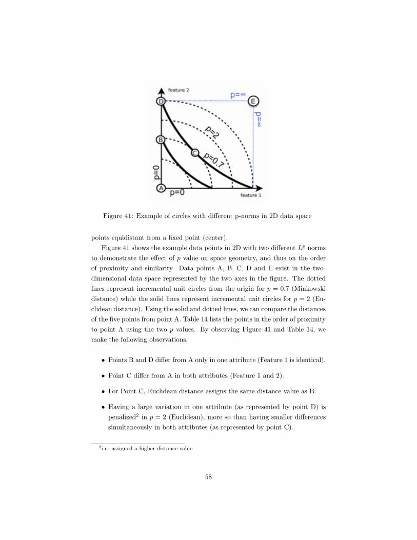
Figure 41: Example of circles with different p-norms in 2D data space
points equidistant from a fixed point (center).Figure 41 shows the example data points in 2D with two different Lp norms
to demonstrate the effect of p value on space geometry, and thus on the orderof proximity and similarity. Data points A, B, C, D and E exist in the two-dimensional data space represented by the two axes in the figure. The dottedlines represent incremental unit circles from the origin for p = 0.7 (Minkowskidistance) while the solid lines represent incremental unit circles for p = 2 (Eu-clidean distance). Using the solid and dotted lines, we can compare the distancesof the five points from point A. Table 14 lists the points in the order of proximityto point A using the two p values. By observing Figure 41 and Table 14, wemake the following observations.
• Points B and D differ from A only in one attribute (Feature 1 is identical).
• Point C differ from A in both attributes (Feature 1 and 2).
• For Point C, Euclidean distance assigns the same distance value as B.
• Having a large variation in one attribute (as represented by point D) ispenalized2 in p = 2 (Euclidean), more so than having smaller differencessimultaneously in both attributes (as represented by point C).
2i.e. assigned a higher distance value
58

Rank p = 2 p = 0.7
1 A A2 B, C B3 D C, D4 E E
Table 14: Ranked distance in two different L
p spaces
Rank Entry Name Distance1 ANETH [PARADOX (DESERT CREEK)] CF24 [CR24] 0.00002 JUDY CREEK [SWAN HILLS (JUDY CREEK A POOL)] CF139 [CR139] 37.67573 MITSUE [WATT MOUNTAIN (GILWOOD A)] SF504 [SR504] 42.01004 NORTH BURBANK [BURBANK (RED FORK)] SF528 [SR528] 42.43615 NIPISI [WATT MOUNTAIN (GILWOOD A POOL)] SF526 [SR526] 44.87406 AL HUWAISAH [SHUAIBA] CF13 [CR13] 45.44057 FULLERTON [WICHITA-CLEARFORK] CF101 [CR101] 45.58808 MABEE [SAN ANDRES] CF184 [CR184] 47.18819 VACUUM [SAN ANDRES] CF319 [CR319] 47.685310 QATIF [ARAB D] CF248 [CR248] 47.8834
Table 15: Top 10 reservoirs selected by Minkowski distance with p = 0.7
In order to give more credit3 to the case of smaller differences in both attributes(as opposed to one larger difference in only one attribute), use Minkowski dis-tance with p = 0.7. By varying the value of p, one can adjust for this effect,the dynamic of which is restated below. This balancing effect works by vary-ing the geometry of the space in which the proximity measure operates, and isgeneralizable for higher order dimensions.
[Large differences in few attributes]
vs.
[Small differences in many attributes]
Ranking by similarity using Minkowski distance with p values of 0.7 and1.5 yields two lists given in Table 15 and Table 16. Also, the data for top 10recommended reservoir entries for both cases are given in Table 15 and Table 16in pages 61 and 62 respectively.
3 i.e. assign a smaller distance value
59

Rank Entry Name Distance1 ANETH [PARADOX (DESERT CREEK)] CF24 [CR24] 0.00002 JUDY CREEK [SWAN HILLS (JUDY CREEK A POOL)] CF139 [CR139] 4.01843 NORTH BURBANK [BURBANK (RED FORK)] SF528 [SR528] 4.37464 NIPISI [WATT MOUNTAIN (GILWOOD A POOL)] SF526 [SR526] 4.44405 MITSUE [WATT MOUNTAIN (GILWOOD A)] SF504 [SR504] 4.47036 SLAUGHTER [SAN ANDRES] CF290 [CR290] 4.50457 VACUUM [SAN ANDRES] CF319 [CR319] 4.58748 PENWELL [SAN ANDRES] CF241 [CR241] 4.74209 EL BORMA [KIRCHAOU] SF243 [SR243] 4.835110 AL HUWAISAH [SHUAIBA] CF13 [CR13] 4.9258
Table 16: Top 10 reservoirs selected by Minkowski distance with p = 1.5
6.5 Conclusions and Discussions for Chapter 6
In this chapter, Euclidean distance, Manhattan distance, and Minkowskidistance were used as measurements of dissimilarity. Each reservoir entry wascompared with all other entries available in the data set using one of the distancemeasures, and the reservoirs were ranked according to the selected reservoir andthe calculated distance. With Minkowski distance, the system users can adjustthe parameter p to vary the extent of the system’s preference between the twoways in which the data can vary. We also discussed the possible use of princi-ple components in the process to reduce or eliminate the effect of intervariatedependencies. Overall, the approach is a systematic way in which data pointsare sorted by similarity, and provides a structured and repeatable method withwhich analog reservoirs can be obtained.
A discussion on the ranked lists is in order. First, it is necessary to pointout that no one selection of distance measure has distinct advantage of another.It is important that the user understands the mechanics of different distancemeasures and use it to his advantage when searching for reservoir analogs.
Another point is that the recommended reservoirs are the most similar tothe selected reservoir, but may not in fact be similar. In other words, thealgorithms only rank the reservoirs in the order of data space proximity; whetherthe reservoirs ranked at the top actually do resemble the target reservoir enoughis left to the user to assess. This idea will be especially applicable if one issearching for analogs for a reservoir that is considered to be an outlier. If thedata sets being used has higher number of entries, it is less likely that one willhave this problem.
60

RA
NK
12
34
56
78
910
WELL_
CO
UN
T_
PR
OD
500
170
700
8910
162
3023
6421
214
8W
ELL_
CO
UN
T_
INJ
500
248
738
240
63
422
STR
UC
T_
CO
MP
RT
_C
OU
NT
11
11
11
11
11
DEP
TH
1676
.426
03.0
1737
.488
3.9
1679
.512
95.4
1554
.515
10.3
2042
.223
98.8
DIP
2.0
0.5
0.5
1.5
0.5
2.2
0.5
1.5
2.0
0.5
AR
EA
195.
312
9.5
566.
691
.038
6.7
29.4
404.
755
.011
9.4
161.
9H
C_
CO
L_
HEIG
HT
_O
IL79
.370
.165
.567
.138
.113
7.2
121.
939
.610
6.7
91.4
HC
_C
OL_
HEIG
HT
79.3
70.1
93.0
67.1
38.1
137.
212
1.9
39.6
106.
710
0.6
STR
AT
I_C
OM
PR
T_
CO
UN
T3
53
34
44
39
4T
HIC
KN
ESS
_G
RO
SS_
AV
G54
.86
70.1
024
.38
30.4
830
.48
112.
7827
4.32
76.2
060
9.60
107.
59N
ET
_G
RO
SS_
RA
TIO
0.45
0.39
0.40
0.70
0.30
0.40
0.49
0.40
0.34
0.50
TH
ICK
NESS
_N
ET
_PA
Y15
.24
18.2
93.
9615
.24
4.27
45.7
221
.34
30.4
845
.72
30.4
8P
OR
OSI
TY
109
1317
1412
1221
1017
K_
AIR
1545
230
5025
017
1060
350
0SW
2316
3630
3116
2030
2220
OO
IP17
5.01
130.
1414
1.76
106.
7613
1.73
99.0
944
6.43
222.
7418
0.58
226.
72O
GIP
0.13
10.
053
0.03
90.
045
0.04
30.
010
0.37
90.
032
0.05
50.
020
CU
M_
OIL
70.6
450
.12
60.7
823
.86
56.3
236
.59
200.
1537
.87
49.4
811
1.37
CU
M_
GA
S0.
0110
0.01
870.
0268
0.01
070.
0092
0.01
520.
0282
0.03
180.
0220
0.02
03A
PI
4141
4139
4138
3040
4242
VIS
C0.
531.
280.
603.
000.
890.
962.
001.
100.
750.
29V
ISC
_T
EM
P50
8960
4949
6642
4947
82G
AS_
SPEC
_G
RAV
0.75
00.
763
0.76
40.
866
0.85
00.
700
0.90
10.
666
0.86
00.
719
FV
F1.
350
1.40
81.
447
1.20
01.
200
1.28
81.
228
1.35
01.
620
1.70
0T
EM
P37
9457
3447
2226
4530
61P
_I
1498
5.51
2417
0.18
1809
3.11
8286
.92
1803
0.96
1124
2.59
1180
8.86
1726
4.42
2057
9.19
2603
4.74
RF_
OIL
_U
LT53
.046
.046
.048
.044
.031
.345
.026
.028
.059
.0R
F_
GA
S_U
LT76
.17
76.3
373
.17
74.3
375
.67
69.0
080
.33
69.6
773
.17
83.3
3W
ELL_
SPA
C_
OIL
0.12
10.
324
1.29
50.
040
0.64
80.
081
0.06
90.
162
0.04
00.
445
WELL_
SPA
C_
GA
S0.
8072
0.74
700.
4858
0.65
780.
6880
0.72
520.
9985
0.52
630.
6950
0.77
57
Tabl
e17
:In
form
atio
non
the
rese
rvoi
rsra
nked
top
10by
Min
kow
skid
ista
nce
wit
hp=
0.7
61

RA
NK
12
34
56
78
910
WELL_
CO
UN
T_
PR
OD
500
170
8910
170
030
2362
164
148
64W
ELL_
CO
UN
T_
INJ
500
27
3848
406
240
223
STR
UC
T_
CO
MP
RT
_C
OU
NT
11
11
11
11
11
DEP
TH
1676
.426
03.0
883.
916
79.5
1737
.415
54.5
1295
.499
0.6
2398
.815
10.3
DIP
2.0
0.5
1.5
0.5
0.5
0.5
2.2
2.0
0.5
1.5
AR
EA
195.
312
9.5
91.0
386.
756
6.6
404.
729
.440
.116
1.9
55.0
HC
_C
OL_
HEIG
HT
_O
IL79
.370
.167
.138
.165
.512
1.9
137.
212
1.9
91.4
39.6
HC
_C
OL_
HEIG
HT
79.3
70.1
67.1
38.1
93.0
121.
913
7.2
121.
910
0.6
39.6
STR
AT
I_C
OM
PR
T_
CO
UN
T3
53
43
44
24
3T
HIC
KN
ESS
_G
RO
SS_
AV
G54
.86
70.1
030
.48
30.4
824
.38
274.
3211
2.78
121.
9210
7.59
76.2
0N
ET
_G
RO
SS_
RA
TIO
0.45
0.39
0.70
0.30
0.40
0.49
0.40
0.49
0.50
0.40
TH
ICK
NESS
_N
ET
_PA
Y15
.24
18.2
915
.24
4.27
3.96
21.3
445
.72
35.9
730
.48
30.4
8P
OR
OSI
TY
109
1714
1312
1211
1721
K_
AIR
1545
5025
023
010
173
500
60SW
2316
3031
3620
1635
2030
OO
IP17
5.01
130.
1410
6.76
131.
7314
1.76
446.
4399
.09
52.3
422
6.72
222.
74O
GIP
0.13
10.
053
0.04
50.
043
0.03
90.
379
0.01
00.
068
0.02
00.
032
CU
M_
OIL
70.6
450
.12
23.8
656
.32
60.7
820
0.15
36.5
916
.55
111.
3737
.87
CU
M_
GA
S0.
0110
0.01
870.
0107
0.00
920.
0268
0.02
820.
0152
0.01
330.
0203
0.03
18A
PI
4141
3941
4130
3839
4240
VIS
C0.
531.
283.
000.
890.
602.
000.
962.
660.
291.
10V
ISC
_T
EM
P50
8949
4960
4266
5882
49G
AS_
SPEC
_G
RAV
0.75
00.
763
0.86
60.
850
0.76
40.
901
0.70
00.
733
0.71
90.
666
FV
F1.
350
1.40
81.
200
1.20
01.
447
1.22
81.
288
1.24
01.
700
1.35
0T
EM
P37
9434
4757
2622
2161
45P
_I
1498
5.51
2417
0.18
8286
.92
1803
0.96
1809
3.11
1180
8.86
1124
2.59
1277
5.67
2603
4.74
1726
4.42
RF_
OIL
_U
LT53
.046
.048
.044
.046
.045
.031
.340
.059
.026
.0R
F_
GA
S_U
LT76
.17
76.3
374
.33
75.6
773
.17
80.3
369
.00
77.1
783
.33
69.6
7W
ELL_
SPA
C_
OIL
0.12
10.
324
0.04
00.
648
1.29
50.
069
0.08
10.
040
0.44
50.
162
WELL_
SPA
C_
GA
S0.
8072
0.74
700.
6578
0.68
800.
4858
0.99
850.
7252
0.50
470.
7757
0.52
63
Tabl
e18
:In
form
atio
non
the
rese
rvoi
rsra
nked
top
10by
Min
kow
skid
ista
nce
wit
hp=
1.5
62

7 Conclusions and Recommendations
The main two objectives of this thesis was 1) to use linear regression, se-quential feature selection, and Bayesian network to create predictive modelsfor reservoirs’ ultimate recovery factors, and 2) to create analog recommendersystems that use various forms of distance measures to rank in the order ofproximity.
For the first objective, the best performance was seen when multilinear re-gression was used in conjunction with sequential forward feature selection. Theperformance of this case was significantly improved from the case where multi-linear regression was conducted using hand-selected variables from the database.In comparison with the multilinear regression with sequential feature selectionmethod, Bayesian network performed poorly. Three tests conducted on simpleBayesian network models revealed that the Bayesian network model not ro-bust, and therefore is unsuitable for the purpose of predicting ultimate recoveryfactors.
For the second objective, we have demonstrated that Euclidean distance,Manhattan distance, and other forms of Minkowski distance can be used todefine similarity to sort reservoirs with. PCA was also employed along withEuclidean distance to create another list of similar reservoirs, which coincidedwell with the lists given by other metrics. There were many overlaps in the listsof top 10 entries for the three methods, suggesting that generally the similarones are listed irrespective of the metric chosen for analysis.
There are two major reasons for the models’ inadequacies: the original dataset and inaccuracies in the model design. The data set does not include somecritical variables—such as time since initial production, or reservoir maturity—whose inclusion may have given statistically significant results. Also, none ofthe variables in the data set are indicators of reservoir heterogeneity, which mayhave a strong correlation with recovery efficiencies. The analysis could improvefurther if the data set included primary, secondary, and ultimate recovery effi-ciencies separately. Finally, if the data set were more complete, then we couldhave relied less on data imputation techniques that may have introduced morenoise to the process than necessary.
The experiments with the Bayesian network are by no means conclusive,because there are many possible permutations. For example, Bayesian networkcould have a more complex structure than a naïve Bayesian network used in thisthesis, or it could include different variables, which may affect performance.
63

Appendix
Drive Mechanism Code DescriptionCOM CombinationDEP DepletionGCP Gas CapPAC Compaction DrivePAR Partial WaterSLG Solution GasUNK UnknownWTR Water Drive
64

8 References
A. Arianfar, B. Khendri, M. H. A. G. M. P. and Z. Mehdipour (2007). Casehistory: Seismic Facies Analysis Based on 3D Multiattribute Volume Classi-fication in Shadegan Oilfield—Asmari Reservoir, Iran. This paper was pre-pared for presentation at the 2007 SPE/EAGE Reservoir Characterizationand Simulation Conference held in Abu Dhabi, U.A.E., 28-31 October 2007.SPE 11078.
Akande, K., S. O. Olantunji, T. Owolabi, and A. AbdulRaheem (2015). Com-parative Analysis of Feature Selection-Based Machine Learning Techniques inReservoir Characterization. Presented at the SPE Saudi Arabia Section An-nual Technical Symposium and Exhibition, Al-Khobar, Saudi Arabia, 21-23April. SPE-178006-MS.
Arps, J. J., F. Brons, A. F. van Everdingen, R. W. Buchwald, and A. E. Smith(1967). A statistical study of recovery efficiency. Bull. D14, API .
Bishop, C. M. (2006). Pattern Recognition and Machine Learning. Cambridge:Springer.
Box, G. E. P. and D. R. Cox (1964). An Analysis of Transformations. Journalof the Royal Statistical Society. Series B (Methodological) 26 (2), 211–252.
Burago, D., Y. Burago, and S. Ivanov (1995). A Course in Metric Geometry.
Carpenter, P., E. Nicholas, and H. M. (2003). Bayesian Belief Networks forPipeline Leak Detection. Presented at the PSIG Annual Meeting held inWilliamsburg, Virginia, 11-13 October. PSIG 0604.
Cofino, A. S.o, A. S., R. Cano, S. C., and G. J. M. (2002). Bayesian Networksfor Probabilistic Weather Prediction. 15th European Conference on ArtificialIntelligence, IOS Press, 695-700.
Council, N. R. (2013). Frontiers in Massive Data Analysis. Washington: TheNational Academies Press.
Devore, J. (2012). Probability and Statistics for Engineering and the Sciences,8th Edition. Boston: Brooks/Cole.
Fisher, D. and H. Lenz (2007). Learning from Data: Artificial Intelligence andStatistics. Springer.
Guthrie, R. K. and M. Greenberger (1955). The Use of Multiple CorrelationAnalysis for Interpreting Petroleum Engineering Data. API Conference Paper,March. API 903-31-G.
65

Hotelling, H. (1933). Analysis of a Complex Statistical Variables into PrincipalComponents. Journal of Educational Psychology. Vol 2 (5): 359-366..
Kita, E., Y. Zuo, M. Harada, and T. Mizuno (2012). Application of BayesianNetwork to Stock Price Prediction.
Koller, D. and N. Friedman (2009). Probabilistic Graphical Models: Principlesand Techniques. The MIT Press.
Kotsiantis, S. B., D. Kanellopoulos, and P. E. Pintelas (2006). Data Prepro-cessing for Supervised Leaning. International Journal of Computer Science 1(2): 1306-4428 .
Kudo, M. and J. Sklansky (2000). Comparison of Algorithms that Select Fea-tures for Pattern Classifiers. Pattern Recognition. Vol 33 (1): 25-41..
Pearl, J. (2009). Causality, 2nd edition. Los Angeles, California: CambridgeUniversity Press.
Rajaieyamchee, M. A., R. B. Bratvold, and A. Badreddine (2010). BayesianDecision Networks for Optimal Placement of Horizontal Wells. Presentedat the SPE EUROPEC/EAGE Annual Conference and Exhibition held inBarcelona, Spain, 14-17 June. SPE 129984.
Rodriguez, M. H., E. Escobar, S. Embid, N. Rodriguez, M. Hegazy, and L. W.Lake (2013). New Approach to Identify Analogue Reservoirs. Presented at theSPE Annual Technical Conference and Exhibition, New Orleans, Louisiana,U.S. 30 September-2 October. SPE-166449.
Sharma, A., S. Srinivasan, and L. W. Lake (2010). Classification of Oil and GasReservoirs Based on Recovery Factor: A Data-Mining Approach. Presented atthe SPE Annual Technical Conference and Exhibition, Florence, Italy, 19-22September. SPE-130257-MS.
Stoian, E. and A. S. Telford (1966). Determination of Natural Gas RecoveryFactors. PETSOC Journal, JCPT 66-03-02 .
Tyler, N. and R. J. Finley (1992). Architectural Controls on the Recovery ofHydrocarbons from Sandstone Reservoirs. In: Miall, A. D. and Tyler, N., TheThree-Dimensional Facies Architecture of Terrigenous Clastic Sediments andIts Implications for Hydrocarbon Discovery and Recovery, SEPM Conceptsin Sedimentology and Palaeontology, 3, Tulsa, pp. 1-5, 1991.
Van Buuren, S. and K. Groothius-Oudshoorn (2009). mice: Multiple Imputationby Chained Equations in R. Journal of Statistical Software Vol 45 Issue 3 .
Venables, W. N. and B. Ripley (1999). Modern Applied Statistics with S-PLUS.Springer. Third Edition.
66

Y. Hajizadeh, E. P. A. and M. C. Souza (2012). Building Trust in History Match-ing: The Role of Multidimensional Projection. Prepared for presentation atthe EAGE Annual Conference & Exhibition incorporating SPE Europec heldin Copenhagen, Denmark, 4-7 June 2012. SPE 152754.
Zerafat, M. M., S. Ayatollahi, N. Mehranbod, and D. Barzegari (2011). BayesianNetwork Analysis as a Tool for Efficient EOR Screening. Presented at theSPE Enhanced Oil Recovery Conference held in Kuala Lumpur, Malaysia,19-21 July. SPE-143282-MS.
67