COPYRIGHT Abraham, B. and Ledolter, J. …statmath.wu-wien.ac.at/~ledolter/AbrahamLedolterRegressionChapter1.pdfon a line with slope one and intercept log(P). ... periods are plotted

COPYRIGHT Abraham, B. and Ledolter, J.

Introduction to Regression Modeling

Belmont, CA: Duxbury Press, 2006

Abraham Abraham˙C01 November 8, 2004 0:33

1 Introduction toRegression Models

1.1 INTRODUCTIONRegression modeling is an activity that leads to a mathematical description ofa process in terms of a set of associated variables. The values of one variablefrequently depend on the levels of several others. For example, the yield of acertain production process may depend on temperature, pressure, catalyst, andthe rate of throughput. The number or the rate of defectives of a process maydepend on the speed of the production line. The number of defective seals ontoothpaste tubes may depend on the temperature and the pressure of the sealingprocess. The volume of a tree is related to the diameter of the tree at breastheight, the height of the tree, and the taper of the tree. The fuel efficiency of anautomobile depends, among others, on the weight of the car and characteristics ofits body and engine. Employee efficiency may be related to the performance onemployment tests, years of training, and educational background. The salaries ofmanagers, athletes, and college teachers may depend on their seniority, the sizeof the market, and their performance. Many additional examples can be given,and in Exercise 1.1 we ask you to comment on several other relationships indetail.

The supply of a product depends on the price customers are willing to pay;one can expect that more products are brought to market when the price is high.Economists refer to this relationship as the production function. Similarly, thedemand for a product depends on the price of the item, the price of the competition,and the amount spent on its advertisement. Economists refer to this relationshipas the demand function. One can expect lower sales if the price is high, in-creased sales if the price of the competition is higher, and increased sales if moremoney is spent on promotion. However, price and advertising may also interact.Advertising may be more effective if the price is low; furthermore, the effect ofthe competition’s price on sales may depend on one’s own price. Also, seasonalcomponents may have an impact on sales during a certain period because sales ofa summer item during winter months will be low in northern states, irrespectiveof the product’s price.

1


2 Introduction to Regression Models

In all these situations we are interested in obtaining a “model” or a “law” (i.e.,a mathematical description) for the relationship among the variables. Regressionanalysis deals with modeling the functional relationship between a responsevariable and one or more explanatory variables. In some instances one has afairly good idea about the form of these models. Often the laws from physics orchemistry tell us how a response is related to the explanatory variables. These lawsmay involve complicated mathematical equations that contain functions such aslogarithms and exponentials. In some instances, the constants in the equationsare also known, but more often the constants need to be determined empiricallyby “fitting” the models to data. In many social science applications, theoreticalmodels are absent, and one must develop empirical models that describe the mainfeatures of the relationship entirely from data.

Let us consider a few illustrative examples in detail.

1.2 EXAMPLES1.2.1 PAYOUT OF AN INVESTMENT

Consider the payout of a principal P that you invest for a certain number of years(length of maturity) T , at an annual interest rate of 100R percent. We know fromsimple actuarial mathematics that the payout is given by

Payout = f (P, R, T ) = P(1 + R)T (1.1)

provided that interest is compounded annually. With continuous compoundingthe resulting payout is slightly different. In this case, it can be calculated fromPayout = PeRT , where e is Euler’s number (e = 2.71828 . . .).

This first example illustrates a deterministic relationship. Each investmentof principal P at rate R and maturity T leads to the exact same payout—nothingmore and nothing less. We are very familiar with this law, and we would notneed any data (or regression methods) to arrive at this particular model. However,assume for a moment that one was unfamiliar with the theory but had data on thepayouts of different investments P , with different interest rates and maturities.Since the relationship is deterministic, payouts from identical investments wouldbe identical and would not provide any additional information. Given this infor-mation, one would—after some trial and error and carefully constructed plots ofthe information—“see” the underlying functional relationship. This model would“fit” the data perfectly.

We have actually used the previous relationship to generate payouts for dif-ferent principals, interest rates, and maturities, and we ask you in Exercise 1.2 todocument the approach you use to find the model. You will experience firsthandthe value of good theory; good theory will avoid much trial and error. Note that forpayouts from continuous compounding, a plot of the logarithm of payout againstthe product of interest rate and length of maturity (RT ) will show points fallingon a line with slope one and intercept log(P).


1.2 Examples 3

1.2.2 PERIOD OF OSCILLATION OF A PENDULUM

Consider the period of oscillation (let us call it µ) of a pendulum of length L . Itis a well-known fact from physics that the period of oscillation is proportional tothe square root of the pendulum’s length L , µ = βL1/2. However, the value of theproportionality factor β may be unknown.

In this example, we are given the functional form of the relationship, butwe are missing information on the key constant, the proportionality factor β.In statistics we refer to unknown constants as parameters. The values of theparameters are usually determined by collecting data and using the resulting datato estimate the parameters.

The situation is also more complicated than in the first example because thereis measurement error. Although the length of the pendulum is easy to measure,the determination of the period of oscillation is subject to variability. This meansthat sometimes our measurement of the “true” period of oscillation is too high andsometimes too low. However, for a calibrated measurement system we can expectthat there is no bias (i.e., on average there is no error). If measured oscillationperiods are plotted against the square roots of varying pendulum lengths, then thepoints will not line up exactly on a straight line through the origin, and there willbe some scatter.

Mathematically, we characterize the relationship between the true periodof oscillation µ and the length of the pendulum L as µ = βL1/2. However, themeasured oscillation period OP is the sum of the true period (which we sometimescall the signal) and the measurement error ε (which we sometimes call the noise).Typically, we use a symmetric distribution about zero for the measurement errorsince the error is supposed to reflect only unbiased variability; if there were somebias in the measurement error, then such bias could be incorporated into the signalcomponent of the model. Combining these two components (the signal and thenoise) leads to the model

OP = µ + ε = βL1/2 + ε (1.2)

This model is similar to the one in Example 1.2.1 because we use theory (inthis case, physics) to suggest the functional form of the relationship. However, incontrast to the previous example, we do not know certain constants (parameters)of the function. These parameters need to be estimated from empirical informa-tion. Furthermore, we have to deal with measurement variability, which leads tovariability (or scatter) around the function (here, a line through the origin). We in-clude a stochastic component ε in the model in order to capture this measurementvariability.

1.2.3 SALARY OF COLLEGE TEACHERS

The third example represents a situation in which there is no theory about thefunctional form of the relationship and there is considerable variability in themeasurements. In this situation, the data must perform “double duty,” namely



to determine the functional form of the model and the values of the parametersin these functions. Moreover, the modeling must be carried out in the presenceof considerable variability. We refer to such models as empirical models (incontrast to the theory-based models discussed in Examples 1.2.1 and 1.2.2), andwe refer to the process of constructing such models as empirical model build-ing. Examples of this type arise in the social sciences, economics, and business,where one usually has little a priori theory of what the functions should looklike.

Consider building a model that explains the annual salary of a college pro-fessor. We probably agree that salary should be related to experience (the moreexperience, the higher the salary), teaching performance (better teachers are paidmore), performance on research (significant papers and books increase the salary),and whether the job includes administrative duties (administrators usually get paidmore). However, we are lacking a theory that tells us the functional form of themodel. Although we know that salary should increase with years of experience,we do not know whether the function should be linear in years, quadratic, orwhether an even more complicated function of the number of years should beused. The same applies to the other variables.

Moreover, we notice considerable variability in salary because professorswith virtually identical background often are paid vastly different salaries. So theremay be additional factors that one has overlooked. Feel free to brainstorm and addto this initial list of variables. For example, salary may also depend on gender andracial factors (use of these factors would be illegal), the year the professor washired, whether the professor is easy to get along with, whether the professor hashad a relationship with the dean’s spouse or had made an inappropriate remarkat last year’s holiday party, and so on. Knowing these factors may improve the fitof the model to the data. However, even after factoring all these variables into themodel, substantial random variation will still exist.

Another aspect that makes the modeling within the social science contextso difficult is problems with measuring the variables. Consider, for example, theteaching performance of an instructor. Although student ratings from end-of-the-semester questionnaires could be used as an indicator of teaching performance,one could argue that these ratings are only a poor proxy. Demanding teachers,difficult subject matter, and lectures held in large classes are known to lowerthese ratings, thus biasing the measure. Assessment of research performance isanother good case in point. One could use the number of publications and booksand use this as a proxy for research. However, such a simple-minded count doesnot incorporate the quality of the publications. Even if one decides to somehowincorporate publication quality, one notices very quickly that reasonable peoplediffer in their judgments. Of course, not being able to accurately measure thefactors that we believe to have an effect on the response affects the results of theempirical modeling.

In summary, we find that empirical modeling faces many difficulties: little orno theory on how the variables fit together, often considerable variability in the


1.2 Examples 5

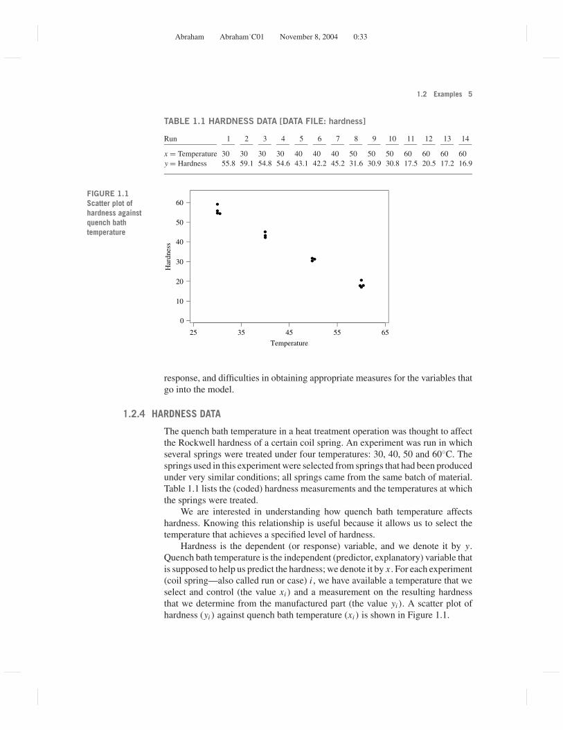
TABLE 1.1 HARDNESS DATA [DATA FILE: hardness]

Run 1 2 3 4 5 6 7 8 9 10 11 12 13 14

x = Temperature 30 30 30 30 40 40 40 50 50 50 60 60 60 60y = Hardness 55.8 59.1 54.8 54.6 43.1 42.2 45.2 31.6 30.9 30.8 17.5 20.5 17.2 16.9

25 35 45 55 65

0

10

20

30

40

50

60

Temperature

Har

dnes

s

FIGURE 1.1Scatter plot ofhardness againstquench bathtemperature

response, and difficulties in obtaining appropriate measures for the variables thatgo into the model.

1.2.4 HARDNESS DATA

The quench bath temperature in a heat treatment operation was thought to affectthe Rockwell hardness of a certain coil spring. An experiment was run in whichseveral springs were treated under four temperatures: 30, 40, 50 and 60◦C. Thesprings used in this experiment were selected from springs that had been producedunder very similar conditions; all springs came from the same batch of material.Table 1.1 lists the (coded) hardness measurements and the temperatures at whichthe springs were treated.

We are interested in understanding how quench bath temperature affectshardness. Knowing this relationship is useful because it allows us to select thetemperature that achieves a specified level of hardness.

Hardness is the dependent (or response) variable, and we denote it by y.Quench bath temperature is the independent (predictor, explanatory) variable thatis supposed to help us predict the hardness; we denote it by x . For each experiment(coil spring—also called run or case) i , we have available a temperature that weselect and control (the value xi ) and a measurement on the resulting hardnessthat we determine from the manufactured part (the value yi ). A scatter plot ofhardness (yi ) against quench bath temperature (xi ) is shown in Figure 1.1.



We want to build a model (i.e., a mathematical relationship) to describe y interms of x . Note that y cannot be a function of x alone since we have observeddifferent y’s (55.8, 59.1, 54.8, and 54.6) for the same x = 30. Furthermore, sinceno theoretical information is available to us to construct the model, we have tostudy the relationship empirically. The scatter plot of y against x indicates that yis approximately linear in x .

The scatter plot suggests the following model:

y(hardness) = β0 + β1x(temperature) + ε (1.3)

where β0 and β1 are the constants (parameters), and ε is the random disturbance(or error) that models the deviations from the straight line. The model is thesum of two components, the deterministic part (or signal) µ = β0 + β1x and therandom part ε. The deterministic part µ = β0 + β1x is a linear function of x withparameters β0 and β1. More important, it is linear in the parameters β0 and β1, andhence we refer to this model as a linear model. The random component ε modelsthe variability in the measurements around the regression line. This variabilitymay come from the measurement error when determining the response y and/orchanges in other variables (other than temperature) that affect the response butare not measured explicitly.

In order to emphasize that the model applies to each considered (and potential)experiment, we introduce subscripts. The temperature and the hardness from theith experiment are written as (xi , yi ). With these subscripts, our model can beexpressed as

yi = β0 + β1xi + εi , where i = 1, 2, . . . , n (1.4)

We complete the model specification by making the following assumptions aboutthe random component ε:

E(εi ) = 0, V (εi ) = σ 2 for all i = 1, 2, . . . , n

εi and ε j are independent random variables for i �= j (1.5)

In this example, we treat xi as deterministic. The experimenter selects thetemperature and knows exactly the temperature of the quench bath. There isno uncertainty about this value. In later sections of this book (Section 2.9), weconsider the case when the values of the explanatory variable are random. Forexample, the observed temperature may only be a “noisy” reading of the truetemperature.

Our assumptions about the error ε and the deterministic nature of the ex-planatory variable x imply that the response yi is a random variable, with meanE(yi ) = µi = β0 + β1xi and variance V (εi ) = σ 2. Furthermore, yi and y j are in-dependent for i �= j .

The mean, E(yi ) = µi = β0 + β1xi , is a linear function of x . The interceptβ0 represents E(y) when x = 0. If the value x = 0 is uninteresting or impossible,the intercept is a rather meaningless quantity. The slope parameter β1 representsthe change in E(y) if x is increased by one unit. For positive β1, the mean E(y)


1.2 Examples 7

TABLE 1.2 UFFI DATA [DATA FILE: uffi]

y = CH2O x = Air Tightness z = UFFI Present

31.33 0 028.57 1 039.95 1 044.98 4 039.55 4 038.29 5 050.58 7 048.71 7 051.52 8 062.52 8 060.79 8 056.67 9 043.58 1 143.30 2 146.16 2 147.66 4 155.31 4 163.32 5 159.65 5 162.74 6 160.33 6 153.13 7 156.83 9 170.34 10 1

increases for increasing x (and decreases for decreasing x). For negative β1, themean E(y) decreases for increasing x and increases for decreasing x .

Our assumption in Eq. (1.5) implies that V (y) = σ 2 is the same for each x .This states that if we repeat experiments at a value of x (as is the case in thisexample), we should see roughly the same scatter at each of the considered x’s.Figure 1.1 shows that the variability in hardness at the four levels of temperature—x = 30, 40, 50, and 60—is about the same.

1.2.5 UREA FORMALDEHYDE FOAM INSULATION

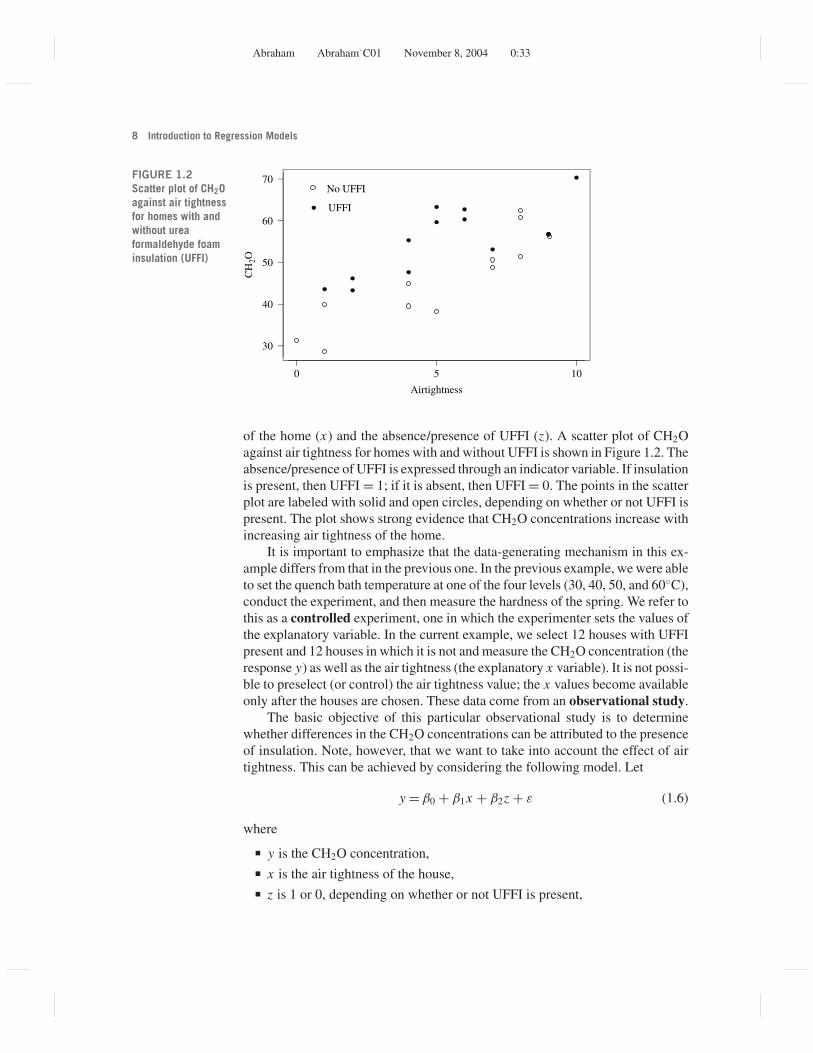
Data were collected to check whether the presence of urea formaldehyde foam in-sulation (UFFI) has an effect on the ambient formaldehyde concentration (CH2O)inside the house. Twelve homes with and 12 homes without UFFI were studied,and the average weekly CH2O concentration (in parts per billion) was measured.It was thought that the CH2O concentration was also influenced by the amountof air that can move through the house via windows, cracks, chimneys, etc. Ameasure of “air tightness,” on a scale of 0 to 10, was determined for each home.

The data are shown in Table 1.2. CH2O concentration is the response variable(y) that we try to explain through two explanatory variables: the air tightness



1050

70

60

50

40

30

Airtightness

CH

2O

No UFFI

UFFI

FIGURE 1.2Scatter plot of CH2Oagainst air tightnessfor homes with andwithout ureaformaldehyde foaminsulation (UFFI)

of the home (x) and the absence/presence of UFFI (z). A scatter plot of CH2Oagainst air tightness for homes with and without UFFI is shown in Figure 1.2. Theabsence/presence of UFFI is expressed through an indicator variable. If insulationis present, then UFFI = 1; if it is absent, then UFFI = 0. The points in the scatterplot are labeled with solid and open circles, depending on whether or not UFFI ispresent. The plot shows strong evidence that CH2O concentrations increase withincreasing air tightness of the home.

It is important to emphasize that the data-generating mechanism in this ex-ample differs from that in the previous one. In the previous example, we were ableto set the quench bath temperature at one of the four levels (30, 40, 50, and 60◦C),conduct the experiment, and then measure the hardness of the spring. We refer tothis as a controlled experiment, one in which the experimenter sets the values ofthe explanatory variable. In the current example, we select 12 houses with UFFIpresent and 12 houses in which it is not and measure the CH2O concentration (theresponse y) as well as the air tightness (the explanatory x variable). It is not possi-ble to preselect (or control) the air tightness value; the x values become availableonly after the houses are chosen. These data come from an observational study.

The basic objective of this particular observational study is to determinewhether differences in the CH2O concentrations can be attributed to the presenceof insulation. Note, however, that we want to take into account the effect of airtightness. This can be achieved by considering the following model. Let

y = β0 + β1x + β2z + ε (1.6)

where

� y is the CH2O concentration,� x is the air tightness of the house,� z is 1 or 0, depending on whether or not UFFI is present,


1.2 Examples 9

� ε is the error component that measures the random component, and� β0, β1, and β2 are constants (parameters) to be estimated.

CH2O concentration is the response variable (y). It is the sum of a deter-ministic component (β0 + β1x + β2z) and a random component ε. The randomcomponent ε is again modeled by a random variable with E(ε) = 0 and V (ε) = σ 2;it describes the variation in the CH2O concentration among homes with identi-cal values for x and z. Large variation in CH2O concentration y among homeswith the same insulation and tightness is characterized by large values of σ 2. Thevariability arises because of measurement errors (it is difficult to measure CH2Oaccurately) and because of other aspects of the house (beyond air tightness andthe presence of UFFI insulation) that have an influence on the response but arenot part of the available information.

The deterministic component, β0 + β1x + β2z, is the sum of three parts.The intercept β0 measures the average CH2O concentration for completely air-tight houses (x = 0) without UFFI insulation (z = 0). The parameter β2 can beexplained as follows: Consider two houses with the same value for air tight-ness (x), the first house with UFFI (z = 1) and the second house without it (z = 0).Then β2 = E(y | house 1) −E(y | house 2) represents the difference in the averageCH2O concentrations for two identical houses (as far as air tightness is concerned)with and without UFFI. This is exactly the quantity we are interested in. If β2 = 0,we cannot link the formaldehyde concentration to the presence of UFFI.

Similarly, β1 is the expected change in CH2O concentrations that is due toa unit change in air tightness in homes with (or without) UFFI. Model (1.6)assumes that this change is the same for homes with and without UFFI. This is aconsequence of the additive structure of the model: The contributions of the twoexplanatory variables, β1x and β2z, get added. However, additivity does not haveto be the rule. The more general model that involves the product of x and z,

y = β0 + β1x + β2z + β3xz + ε (1.7)

allows air tightness to affect the two types of homes differently. For a housewithout UFFI, E(y) = β0 + β1x , and β1 expresses the effect on the CH2O con-centrations of a unit change in air tightness. For a house with UFFI, E(y) =(β0 + β2) + (β1 + β3)x , and (β1 + β3) expresses the effect of a unit change inair tightness. The effect is now different by the factor β3.

1.2.6 ORAL CONTRACEPTIVE DATA

An experiment was conducted to determine the effects of five different oral con-traceptives (OCs) on high-density lipocholesterol (HDLC), a substance found inblood serum. It is believed that high levels of this substance (the “good” choles-terol) help delay the onset of certain heart diseases. In the experiment, 50 womenwere randomly divided into five equal-sized groups; 10 women were assignedto each OC group. An initial baseline HDLC measurement was taken on eachsubject before oral contraceptives were started. After having used the respective



TABLE 1.3 ORAL CONTRACEPTIVE DATA [DATA FILE: contraceptive]

OC1 OC1 OC2 OC2 OC3 OC3 OC4 OC4 OC5 OC5y = Final HDLC z = Initial HDLC y z y z y z y z

43 49 58 56 100 102 50 57 41 3761 73 46 49 52 64 50 55 58 6045 55 66 64 49 60 52 64 58 3946 55 59 63 51 51 58 49 69 6059 63 71 90 48 59 65 78 68 7157 53 64 56 51 57 71 63 64 6356 51 53 46 40 63 52 62 46 5168 74 50 64 52 62 49 50 56 6446 58 68 75 44 61 49 60 51 4547 41 35 58 50 58 58 59 57 58

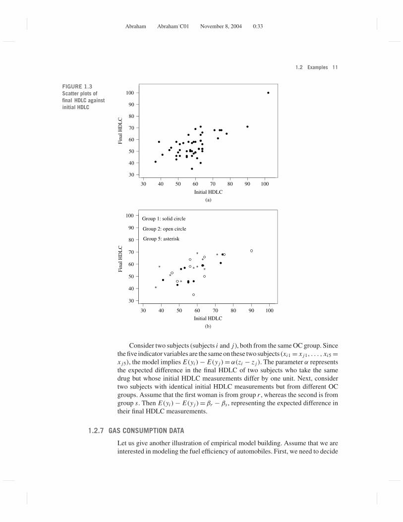
drug for 6 months, a second HDLC measurement was made. The objective ofthe experiment was to study whether the five oral contraceptives differ in theireffect on HDLC. The data are shown in Table 1.3. A scatter plot of final HDLCagainst the initial readings, ignoring the information on the respective treatmentgroups, is shown in Figure 1.3a. Figure 1.3b repeats this graph for groups 1, 2,and 5, using different plotting symbols to denote the three OC groups. Such agraph can highlight potential differences among the groups. (In order to keep thegraph simple, only three groups are shown in Figure 1.3b).

Let yi be the final HDLC measurement on subject i(i = 1, 2, . . . , 50) andlet zi be the initial HDLC reading. Furthermore, define five indicator variablesx1, . . . , x5 so that

xik = 1 if subject i is a participant in the kth OC group

= 0 otherwise

Here, we need two subscripts because there are five x variables. The first index inthis double-subscript notation refers to the subject or case i; the second subscriptrefers to the explanatory variable (OC group) that is being considered. The fol-lowing model relates the final HDLC measurement to six explanatory variables:the initial HDLC reading (z) and the five indicator variables (x1, . . . , x5). Forsubject i ,

yi = αzi + β1xi1 + β2xi2 + · · · + β5xi5 + εi (1.8)

The usual assumption on the random component specifies that E(εi ) = 0 andV (εi ) = σ 2 for all i, and that εi and ε j , for two different subjects i �= j , areindependent.

The deterministic component of the model, E(yi ) = αzi + β1xi1 + β2xi2 +· · · + β5xi5, represents five parallel lines in a graph of E(yi ) against the initialHDLC, zi . The six parameters can be interpreted as follows: The parameter α

represents the common slope. The coefficients β1, β2, . . . , β5 represent the in-tercepts of the five lines and measure the effectiveness of the five OC treatmentgroups. Their comparison is of primary interest because there is no differenceamong the five drugs when β1 = β2 = · · · = β5.


1.2 Examples 11

100908070

(a)

60504030

100

90

80

70

60

50

40

30

Initial HDLC

Fina

l HD

LC

10090807060504030

100

90

80

70

60

50

40

30

Initial HDLC

Fina

l HD

LC

Group 5: asterisk

Group 2: open circle

Group 1: solid circle

(b)

FIGURE 1.3Scatter plots offinal HDLC againstinitial HDLC

Consider two subjects (subjects i and j), both from the same OC group. Sincethe five indicator variables are the same on these two subjects (xi1 = x j1, . . . , xi5 =x j5), the model implies E(yi ) − E(y j ) = α(zi − z j ). The parameter α representsthe expected difference in the final HDLC of two subjects who take the samedrug but whose initial HDLC measurements differ by one unit. Next, considertwo subjects with identical initial HDLC measurements but from different OCgroups. Assume that the first woman is from group r , whereas the second is fromgroup s. Then E(yi ) − E(y j ) = βr − βs , representing the expected difference intheir final HDLC measurements.

1.2.7 GAS CONSUMPTION DATA

Let us give another illustration of empirical model building. Assume that we areinterested in modeling the fuel efficiency of automobiles. First, we need to decide



how to measure fuel efficiency. A typical measure of fuel efficiency used by theEnvironmental Protection Agency (EPA) and car manufacturers is “miles/gallon.”It expresses how many miles a car can travel on 1 gallon of fuel. However, there isan alternative way to express fuel efficiency considering gallons per 100 traveledmiles, “gallons/100 miles.” It expresses the amount of fuel that is needed to travel100 miles. The second measure is the scaled reciprocal of the first: [gallons/100 miles] = 100/[miles/gallon]. In Chapter 6, we discuss how to intelligentlychoose among these two measures. Assume for the time being, that we havesettled on the second measure, [gallons/100 miles].

Next, we need to think about characteristics of the car that can be expected tohave an impact on fuel efficiency. Weight of the car is probably the first variablethat comes to mind. Weight should have the biggest impact, as we know fromphysics that we need a certain force to push an object, and that force is relatedto the fuel input. Heavy cars require more force and, hence, more fuel. Size(displacement) of the engine probably matters also. So does, most likely, thenumber of cylinders, horsepower, the presence of an automatic transmission,acceleration from 0 to 60 mph, the wind resistance of the car, and so on. However,how many explanatory variables should be in the model, and in what functionalform should fuel consumption be related to the explanatory variables? Theorydoes not help much, except that physics seems to imply that [gallons/100 miles]should be related linearly to weight. However, how the other variables enter intothe model and whether there should be interaction effects (e.g., whether changesin weight affect fuel efficiency differently depending on whether the car has asmall or large engine) are open questions.

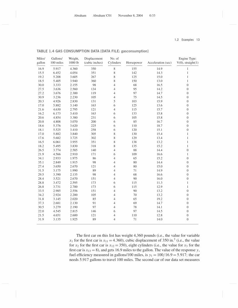
Assume, for the sake of this introductory discussion, that we have settledon the following three explanatory variables: x1 = weight, x2 = engine displace-ment, and x3 = number of cylinders. Table 1.4 lists the fuel efficiency and thecharacteristics of a sample of 38 cars. We assume that the data are a representa-tive sample (random sample) from a larger population. You can always replicatethis study by going to recent issues of Consumer Reports and selecting anotherrandom sample. If you have ample time, you can select all given cars and studythe population. The fact that we are dealing with a random sample is very im-portant because we want to extend any conclusions from the analysis of these 38cars to the larger population at hand. Our results should not be restricted to justthis one set of 38 cars, but our conclusions on fuel efficiency should apply moregenerally to the population from which this sample was taken. If our set of 38cars is not a representative sample, then it is questionable whether the inferencecan be extended to the population.

Note that fuel consumption in Table 1.4 is given in “miles/gallon” and“gallons/100 miles.” Convince yourself that the entries in the second column areobtained through the simple transformation, [gallons/100 miles] = 100/[miles/gallon]. In addition to data on weight, engine displacement, and number ofcylinders, the table includes several other variables that we will use in laterchapters.


1.2 Examples 13

TABLE 1.4 GAS CONSUMPTION DATA [DATA FILE: gasconsumption]

Miles/ Gallons/ Weight, Displacement No. of Engine Type:gallon 100 miles 1000 lb (cubic inches) Cylinders Horsepower Acceleration (sec) V(0), straight(1)

16.9 5.917 4.360 350 8 155 14.9 115.5 6.452 4.054 351 8 142 14.3 119.2 5.208 3.605 267 8 125 15.0 118.5 5.405 3.940 360 8 150 13.0 130.0 3.333 2.155 98 4 68 16.5 027.5 3.636 2.560 134 4 95 14.2 027.2 3.676 2.300 119 4 97 14.7 030.9 3.236 2.230 105 4 75 14.5 020.3 4.926 2.830 131 5 103 15.9 017.0 5.882 3.140 163 6 125 13.6 021.6 4.630 2.795 121 4 115 15.7 016.2 6.173 3.410 163 6 133 15.8 020.6 4.854 3.380 231 6 105 15.8 020.8 4.808 3.070 200 6 85 16.7 018.6 5.376 3.620 225 6 110 18.7 018.1 5.525 3.410 258 6 120 15.1 017.0 5.882 3.840 305 8 130 15.4 117.6 5.682 3.725 302 8 129 13.4 116.5 6.061 3.955 351 8 138 13.2 118.2 5.495 3.830 318 8 135 15.2 126.5 3.774 2.585 140 4 88 14.4 021.9 4.566 2.910 171 6 109 16.6 134.1 2.933 1.975 86 4 65 15.2 035.1 2.849 1.915 98 4 80 14.4 027.4 3.650 2.670 121 4 80 15.0 031.5 3.175 1.990 89 4 71 14.9 029.5 3.390 2.135 98 4 68 16.6 028.4 3.521 2.670 151 4 90 16.0 028.8 3.472 2.595 173 6 115 11.3 126.8 3.731 2.700 173 6 115 12.9 133.5 2.985 2.556 151 4 90 13.2 034.2 2.924 2.200 105 4 70 13.2 031.8 3.145 2.020 85 4 65 19.2 037.3 2.681 2.130 91 4 69 14.7 030.5 3.279 2.190 97 4 78 14.1 022.0 4.545 2.815 146 6 97 14.5 021.5 4.651 2.600 121 4 110 12.8 031.9 3.135 1.925 89 4 71 14.0 0

The first car on this list has weight 4,360 pounds (i.e., the value for variablex1 for the first car is x11 = 4.360), cubic displacement of 350 in.3 (i.e., the valuefor x2 for the first car is x12 = 350), eight cylinders (i.e., the value for x3 for thefirst car is x13 = 8), and gets 16.9 miles to the gallon. The value of the response y,fuel efficiency measured in gallons/100 miles, is y1 = 100/16.9 = 5.917; the carneeds 5.917 gallons to travel 100 miles. The second car of our data set measures



at x21 = 4.054, x22 = 351, x23 = 8, and y2 = 100/15.5 = 6.452 (i.e., weight 4,054pounds, 351 in.3 displacement, eight cylinders, and 6.452 gallons/100 miles).The last car (car 38) measures at x38,1 = 1.925, x38,2 = 89, x38,3 = 4, and y38 =100/31.9 = 3.135 (i.e., weight 1,925 pounds, 89 in.3 displacement, four cylinders,and 3.135 gallons/100 miles).

Observe the notation that we use throughout this book. For the ith unit (inthis case, the car), the values of the explanatory variables x1, x2, . . . , x p (here,p = 3) and the response y are denoted by xi1, xi2, . . . , xip, and yi . Usually, thereare several explanatory variables, not just one. Hence, we must use a double-index notation for xi j , where the first index i = 1, 2, . . . , n refers to the case, andthe second index j = 1, 2, . . . , p refers to the explanatory variable. For example,x52 = 98 is the value of the second explanatory variable (displacement, x2) of thefifth car. Since we are dealing with a single response variable y, there is only oneindex (for case) in yi .

A reasonable starting model relates fuel efficiency (gallons/100 miles) to theexplanatory variables in a linear fashion. That is,

y = µ + ε = β0 + β1x1 + β2x2 + β3x3 + ε (1.9)

As before, the dependent variable is the sum of a random component, ε, and adeterministic component, µ = β0 + β1x1 + β2x2 + β3x3, which is linear in theparameters β0, β1, β2, and β3.

Cars with the same weight, same engine displacement, and the same numberof cylinders can have different gas consumption. This variability is described by ε,which is taken as a random variable with E(ε) = 0 and V (ε) = σ 2. If we considercars with the same weight, same engine displacement, and same number of cylin-ders, then the average deviation from the mean value in gas consumption of these“alike” cars is zero. The variance σ 2 provides a measure of the variability aroundthe mean value. Furthermore, we assume that E(ε) = 0 and V (ε) = σ 2 is the samefor all groups of cars with identical values on x1, x2, and x3. The variability isthere because of measurement variability in determining the gas consumption.However, it also arises because of the presence of other characteristics of the carthat affect fuel consumption but are not part of the data set. Cars may differ withrespect to such omitted variables. If the omitted factors affect fuel consumption,then the fuel consumption of cars that are identical on the measured factors willbe different.

The deterministic component µ = β0 + β1x1 + β2x2 + β3x3 is linear in theparameters β0, β1, β2, and β3. We expect a positive value for the coefficient β1

because a heavier car (with fixed engine displacement and number of cylinders)needs more fuel. Similarly, we expect a positive coefficient β2 because a largerengine on a car of fixed weight and number of cylinders should require more fuel.We also expect a positive coefficient for β3 because more cylinders on a car offixed weight and engine displacement should require more fuel.

In order to understand the deterministic component µ more fully, considertwo cars i and j with identical engine displacement and number of cylinders.


1.3 A General Model 15

Since xi2 = x j2 and xi3 = x j3, the difference

E(yi ) − E(y j ) = β1(xi1 − x j1)

Thus, β1 represents the difference in the mean values of y (the mean difference inthe gas consumption) of two cars whose weights (x1) differ by one unit but thathave the same engine displacement (x2) and the same number of cylinders (x3).Similarly, β2 represents the difference in the mean values of y of two cars whoseengine displacements (x2) differ by one unit but that have the same weight (x1)

and the same number of cylinders (x3). The parameter β3 represents the differencein the mean values of y of two cars whose number of cylinders (x3) differ by oneunit but that have the same weight (x1) and the same engine displacement (x2).

In the modeling context, one often is not certain whether the variables underconsideration are important or not. For instance, we might be interested in thequestion whether or not x3 (number of cylinders) is necessary to predict y (gasconsumption) once we have included the weight x1 and the engine displacementx2 in the model. Thus, we are interested in a test of the hypothesis that β3 = 0,given that x1 and x2 are in the model. Such tests may lead to the exclusion ofcertain variables from the model. On the other hand, other variables such ashorsepower x4 may be important and should be included. Then the model needsto be extended so that its predictive capability is increased.

The model in Eq. (1.9) is quite simple and should provide a useful startingpoint for our modeling. Of course, we do not know the values of the modelcoefficients, nor do we know whether the functional representation is appropriate.For that we need data. One must keep in mind that there are only 38 observationsand that one cannot consider models that contain too many unknown parameters.A reasonable strategy starts with simple parsimonious models such as the onespecified here and then checks whether this representation is capable of explainingthe main features of the data. A parsimonious model is simple in its structureand economical in terms of the number of unknown parameters that need to beestimated from data, yet capable of representing the key aspects of the relationship.We will say more on model building and model checking in subsequent chapters.The introduction in this chapter is only meant to raise these issues.

1.3 A GENERAL MODELIn all of our examples, we have looked at situations in which a single responsevariable y is modeled as

y = µ + ε (1.10a)

The deterministic component µ is written as

µ = β0 + β1x1 + β2x2 + · · · + βpx p (1.10b)

where x1, x2, . . . , x p are p explanatory variables. We assume that the explana-tory variables are “fixed”—that is, measured without error. The parameter



βi (i = 1, 2, . . . , p) is interpreted as the change in µ when changing xi by oneunit while keeping all other explanatory variables the same.

The random component ε is a random variable with zero mean, E(ε) = 0,

and variance V (ε) = σ 2 that is constant for all cases and that does not depend onthe values of x1, x2, . . . , x p. Furthermore, the errors for different cases, εi and ε j ,are assumed independent. Since the response y is the sum of a deterministic anda random component, we find that E(y) = µ and V (y) = σ 2.

We refer to the model in Eq. (1.10) as linear in the parameters. To explain theidea of linearity more fully, consider the following four models with deterministiccomponents:

i. µ = β0 + β1x

ii. µ = β0 + β1x1 + β2x2(1.11)

iii. µ = β0 + β1x + β2x2

iv. µ = β0 + β1 exp(β2x)

Models (i)–(iii) are linear in the parameters since the derivatives of µ with re-spect to the parameters βi , ∂µ/∂βi , do not depend on the parameters. Model(iv) is nonlinear in the parameters since the derivatives ∂µ/∂β1 = exp(β2x) and∂µ/∂β2 = β1x exp(β2x) depend on the parameters.

The model in Eqs. (1.10a) and (1.10b) can be extended in many differentways. First, the functional relationship may be nonlinear, and we may considera model such as that in Eq. (1.11iv) to describe the nonlinear pattern. Second,we may suppose that V (y) = σ 2(x) is a function of the explanatory variables.Third, responses for different cases may not be independent. For example, wemay model observations (e.g., on weight) that are taken on the same subject overtime. Measurements on the same subject taken close together in time are clearlyrelated, and the assumption of independence among the errors is violated. Fourth,several different response variables may be measured on each subject, and wemay want to model these responses simultaneously. Many of these extensionswill be discussed in later chapters of this book.

1.4 IMPORTANT REASONS FOR MODELINGStatistical modeling, as discussed in this text, is an activity that leads to a mathe-matical description of a process in terms of the variables of the process. Once asatisfactory model has been found, it can be used for several different purposes.

i. Usually, the model leads to a simple description of the main features of thedata at hand. We learn which of the explanatory variables have an effect onthe response. This tells us which explanatory variables we have to change inorder to affect the response. If a variable does not affect a response, thenthere may be little reason to measure or control it. Not having to keep trackof something that is not needed can lead to significant savings.


1.5 Data Plots and Empirical Modeling 17

ii. The functional relationship between the response and the explanatoryvariables allows us to estimate the response for given values of theexplanatory variables. It makes it possible to infer the response for values ofthe explanatory variables that were not studied directly. It also allows us toask “what if”-type questions. For example, a model for sales can give usanswers to questions of the following form: “What happens to sales if wekeep our price the same, but increase the amount of advertising by 10%?”or “What happens to the gross national product if interest rates decrease byone percentage point?” Knowledge of the relationship also allows us tocontrol the response variable at certain desired levels. Of course, the qualityof answers to such questions depends on the quality of the models that arebeing used.

iii. Prediction of future events is another important application. We may have agood model for sales over time and want to know the likely sales for the nextseveral future periods. We may have developed a good model relating salesat time t to sales at previous periods. Assuming that there is some stabilityover time, we can use such a model for making predictions of future sales.

In some situations, the models seen here are well grounded in theory.However, often theory is lacking and the models are purely descriptive ofthe data that one has collected. When a model lacks a solid theoreticalfoundation, it is questionable whether it is possible to extrapolate the resultsto new cases that are different from the ones occurring in the studied dataset. For example, one would be very reluctant to extrapolate the findings inExample 1.2.4 and predict hardness for springs that were subjected totemperatures that are much higher than 60◦C.

iv. A regression analysis may show that a variable that is difficult andexpensive to measure can be explained to a large extent by variables that areeasy and cheap to obtain. This is important information because we cansubstitute the cheaper measurements for the more expensive ones. It may bequite expensive to determine someone’s body fat because this requires thatthe whole body be immersed in water. It may be expensive to obtain aperson’s bone density. However, variables such as height, weight, andthickness of thighs or biceps are easy and cheap to obtain. If there is a goodmodel that can explain the expensively measured variable through thevariables that are easy and cheap to obtain, then one can save money andeffort by using the latter variables as proxies.

1.5 DATA PLOTS AND EMPIRICAL MODELINGGood graphical displays are very helpful in building models. Let us use thedata in Table 1.4 to illustrate the general approach. Note that with one responseand p explanatory variables, each case (in this situation, each car) represents apoint in (p + 1) dimensional space. Most empirical modeling starts with plotsof the data in a lower dimensional space. Typically, one starts with pairwise



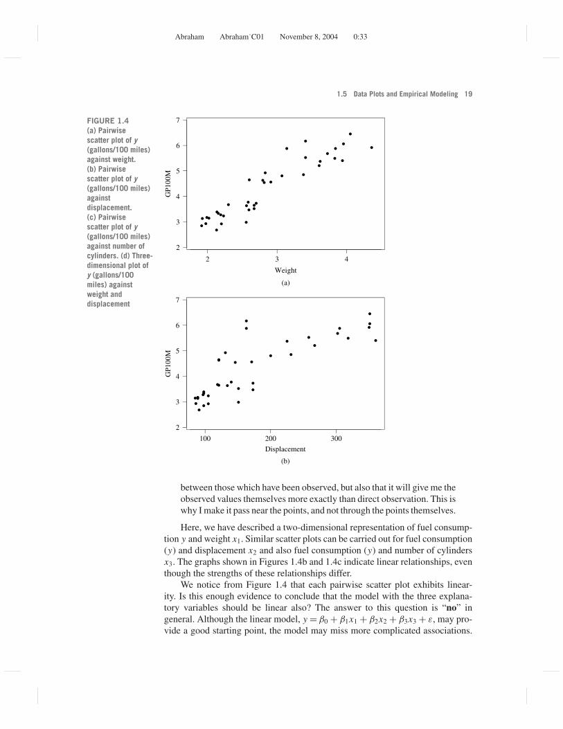
(two-dimensional) scatter plots of the response against each of the explanatoryvariables. The scatter plot of fuel consumption (gallons/100 miles) against weightof the car in Figure 1.4a illustrates that heavier cars require more fuel. It also showsthat the relationship between fuel consumption and weight is well approximatedby a linear function. This is true at least over the observed weight range fromapproximately 2,000 to 4,000 pounds. How the function looks for very light andvery heavy cars is difficult to tell because such cars are not in our group ofconsidered cars; extrapolation beyond the observed range on weight is certainlya very tricky task.

Knowing that this relationship is linear simplifies the interpretation of the re-lationship because each additional 100 pounds of weight increases fuel efficiencyby the same amount, irrespective of whether we talk about a car weighing 2,000or 3,500 pounds. For a quadratic relationship the interpretation would not be asstraightforward because the change in fuel consumption implied by a change inweight from 2,000 to 2,100 pounds would be different than the one implied by achange in weight from 3,500 to 3,600 pounds.

Another notable aspect of the data and the graph in Figure 1.4a is that theobservations do not lie on the line exactly. This is because of variability. Ourmodel recognizes this by allowing for a random component. On average, the fuelefficiency can be represented by a simple straight-line model, but individual ob-servations (the fuel consumption of individual cars) vary around that line. Thisvariation can result from many sources. First, it can be pure measurement error.Measuring the fuel consumption on the very same car for a second time may re-sult in a different number. Second, there is variation in fuel consumption amongcars taken from the very same model line. Despite being from the same modelline and having the same weight, cars are not identical. Third, cars of identicalweight may come from different model lines with very different characteristics.It is not just weight that affects the fuel consumption; other characteristics mayhave an effect. Engine sizes may be different and the shapes may not be thesame. One could make the model more complicated by incorporating these otherfactors into it. Although this would reduce the variability in fuel consumption,one should not make the function so complicated that it passes through everysingle point. Such an approach would ignore the natural variability in measure-ments and attach too much importance to random variation. Henri Poincare, inThe Foundations of Science [Science Press, New York, 1913 (reprinted 1929),p. 169] expresses this very well when he writes,

Pass to an example of a more scientific character. I wish to determinean experimental law. This law, when I know it, can be represented by acurve. I make a certain number of isolated observations; each of thesewill be represented by a point. When I have obtained these differentpoints, I draw a curve between them, striving to pass as near to them aspossible and yet preserve for my curve a regular form, without angularpoints, or inflections too accentuated, or brusque variation of the radiusof curvature. This curve will represent for me the probable law, and Iassume not only that it will tell me the values of the function intermediate


1.5 Data Plots and Empirical Modeling 19

43

(a)

2

7

6

5

4

3

2

Weight

GP1

00M

100 200

(b)

300

2

3

4

5

6

7

Displacement

GP1

00M

FIGURE 1.4(a) Pairwisescatter plot of y(gallons/100 miles)against weight.(b) Pairwisescatter plot of y(gallons/100 miles)againstdisplacement.(c) Pairwisescatter plot of y(gallons/100 miles)against number ofcylinders. (d) Three-dimensional plot ofy (gallons/100miles) againstweight anddisplacement

between those which have been observed, but also that it will give me theobserved values themselves more exactly than direct observation. This iswhy I make it pass near the points, and not through the points themselves.

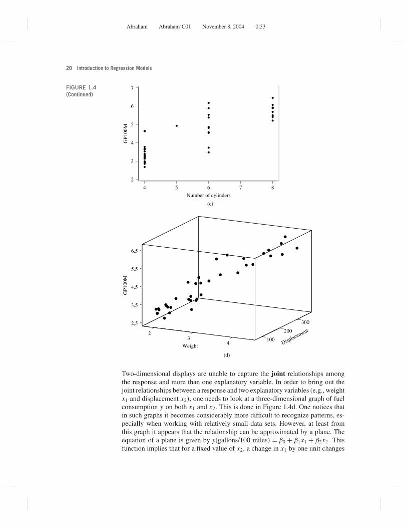
Here, we have described a two-dimensional representation of fuel consump-tion y and weight x1. Similar scatter plots can be carried out for fuel consumption(y) and displacement x2 and also fuel consumption (y) and number of cylindersx3. The graphs shown in Figures 1.4b and 1.4c indicate linear relationships, eventhough the strengths of these relationships differ.

We notice from Figure 1.4 that each pairwise scatter plot exhibits linear-ity. Is this enough evidence to conclude that the model with the three explana-tory variables should be linear also? The answer to this question is “no” ingeneral. Although the linear model, y = β0 + β1x1 + β2x2 + β3x3 + ε, may pro-vide a good starting point, the model may miss more complicated associations.



4 5 6

(c)

7 8

2

3

4

5

6

7

Number of cylinders

GP1

00M

300

2

2.5

Displacement200

3.5

4.5

5.5

3

6.5

GP1

00M

4

(d)

100Weight

FIGURE 1.4(Continued)

Two-dimensional displays are unable to capture the joint relationships amongthe response and more than one explanatory variable. In order to bring out thejoint relationships between a response and two explanatory variables (e.g., weightx1 and displacement x2), one needs to look at a three-dimensional graph of fuelconsumption y on both x1 and x2. This is done in Figure 1.4d. One notices thatin such graphs it becomes considerably more difficult to recognize patterns, es-pecially when working with relatively small data sets. However, at least fromthis graph it appears that the relationship can be approximated by a plane. Theequation of a plane is given by y(gallons/100 miles) = β0 + β1x1 + β2x2. Thisfunction implies that for a fixed value of x2, a change in x1 by one unit changes


1.6 An Iterative Model Building Approach 21

the response y by β1 units. Similarly, for a fixed value of x1, a change in x2 byone unit changes the response y by β2 units. The effects of changes in x1 and x2

are additive. Additivity is a special feature of this particular representation. It isa convenient simplification but need not be true in general. For some relation-ships the effects of a change in one explanatory variable depend on the value ofa second explanatory variable. One says that the explanatory variables interactin how they affect the response y.

Up to now, we have incorporated the effects of x1 and x2. What about the effectof the third explanatory variable x3? It is not possible to display all four variablesin a four-dimensional graph. However, judging from the pairwise scatterplots andthe three-dimensional representations (y, x1, x2), (y, x1, x3), and (y, x2, x3), ourlinear model in x1, x2, and x3 may provide a sensible starting point.

1.6 AN ITERATIVE MODEL BUILDING APPROACHAn understanding of relationships can be gained in several different ways. Onecan start from a well-developed theory and use the data mostly for the estimationof unknown parameters and for checking whether the theory is consistent with theempirical information. Of course, any inconsistencies between theory and datashould lead to a refinement of the model and a subsequent check whether therevised theory is consistent with the data.

Another approach, and one that is typically used in the social sciences, is tostart from the data and use an empirical modeling approach to derive a modelthat provides a reasonable characterization of the relationship. Such a model mayin fact lead to a new theory. Of course, theories must be rechecked against newdata, and in cases of inconsistencies with the new information, new models mustbe developed, estimated, and checked again. Notice that good model building isa continual activity. It does not matter much whether one starts from theory orfrom data; what matters is that this process continues toward convergence.

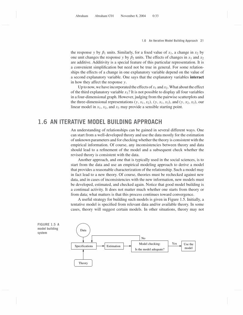
A useful strategy for building such models is given in Figure 1.5. Initially, atentative model is specified from relevant data and/or available theory. In somecases, theory will suggest certain models. In other situations, theory may not

Data

Specifications EstimationModel checking:

No

Yes Use themodel

Theory

Is the model adequate?

FIGURE 1.5 Amodel buildingsystem



exist or may be incomplete, and data must be used to specify a reasonable initialmodel; exploratory data analysis and innovative ways of displaying informationgraphically are essential. The tentatively entertained model usually contains un-known parameters that need to be estimated. Model fitting procedures, such asleast squares or maximum likelihood, have been developed for this purpose.This is discussed further in the next chapter.

Finally, the modeler must check the adequacy of the fitted model. Inadequacycan occur in several ways. For example, the model may miss important variables, itmay include inappropriate and unnecessary variables that make the interpretationof the model difficult, and the model may misspecify the functional form. If themodel is inadequate, then it needs to be changed, and the iterative cycle of “modelspecification—parameter estimation—model checking” must be repeated. Oneneeds to do this until a satisfactory model is obtained.

1.7 SOME COMMENTS ON DATAThis discussion shows that good data are an essential component of any modelbuilding. However, not all data are alike, and we should spend some time dis-cussing various types of data. We should distinguish between data arising fromdesigned experiments and data from observational studies.

Many data sets in the physical sciences are the result of designed studies thatare carefully planned and executed. For example, an engineer studying the impactof pressure and temperature on the yield of a production process may manufactureseveral products under varying levels of pressure and temperature. He or she mayselect three different pressures and four different settings for temperature andconduct one or several experiments at each of the (3) × (4) = 12 different factor-level combinations. A good experimenter will suspect that other factors mayhave an impact on the yield but may not know for sure which ones. It could bethe purity of the raw materials, environmental conditions in the plant during themanufacture, and so on. In order to minimize the effects of these uncontrolledfactors, the investigator will randomize the arrangement of the experimental runs.He or she will do this to minimize the effects of unknown time trends. For example,one certainly would not want to run all experiments with the lowest temperature onone day and all experiments using the high temperature on another. If the processis sensitive to daily fluctuations in plant conditions, an observed difference in theresults of the two days may not be due to temperature but due to the differentconditions in the plant. Good experimenters will be careful when changing thetwo factors of interest, keeping other factors as uniform as possible. What isimportant is that the experimenter is actively involved in all aspects of obtainingthe data.

Observational data are different because the investigator has no way of im-pacting the process that generates the data. The data are taken just as the data-generating process is providing them. Observational data are often referred to as“happenstance” data because they just happen to be available for analysis.


Exercises 23

Economic and social science information is usually collected through a cen-sus (i.e., every single event is recorded) or through surveys. The problem withmany social science data sets is that several things may have gone wrong duringthe data-gathering process, and the analyst has no chance to recover from theseproblems. A survey may not be representative of the population that one wantsto study. Data definitions may not match exactly the factors that one wants tomeasure, and the gathered data may be poor proxies at best. Data quality maybe poor because there may not have been enough time for careful data collectionand processing. There may be missing data. The data that come along may notbe “rich” enough to separate the effects of competing factors.

Consider the following example as an illustration. Assume that you want toexplain college success as measured by student grade point average. Your admis-sion office provides the student ACT scores (on tests taken prior to admission),and you have survey data on the number of study hours per week. Does thisinformation allow you to develop a good model for college success? Yes, to acertain degree. However, there are also significant problems. First, college GPAis quite a narrow definition of college success. GPA figures are readily available,but one needs to discuss whether this is the information one really wants. Sec-ond, the range of ACT scores may be not wide enough to find a major impactof ACT scores on college GPA. Most good universities do not accept marginalstudents with low ACT scores. As a consequence, the range of ACT scores atyour institution will be narrow, and you will not see much effect over that limitedrange. Third, study hours are self-reported, and students may have a tendency tomake themselves look better than they really are. Fourth, ACT scores and studyhours tend to be correlated. Students with a high ACT scores tend to have goodstudy skills; it will be rare to find someone with a very high ACT score who doesnot study. The correlation between the two explanatory variables, ACT score andstudy hours, makes it difficult to separate the effects on college GPA of ACTscores and study hours.

EXERCISES

1.1. Consider the following relationships.Comment on the type of relationships thatcan be expected, supporting your discussionwith simple graphs. In which of these casescan you run experiments that can help youlearn about the relationship between theresponse y and the explanatory variables x?

a. Tensile strength of an alloy may be relatedto hardness and density of the stock.

b. Tool life may depend on the hardness ofthe material to be machined and the depthof the cut.

c. The weight of the coating of electrolytictin plate may be affected by the current,acidity, rate of travel of the strip, anddistance from the anode.

d. The diameter of a condenser coil may beaffected by the thickness of the coil,number of turns, and tension in thewinding.

e. The moisture content of lumber maydepend on the speed of drying, the dryingtemperature, and the dimension of thepieces.



f. The performance of a foundry may beaffected by atmospheric conditions.

g. The life of a light bulb may vary with thequality of the filament; the tile finish maydepend on the temperature of firing.

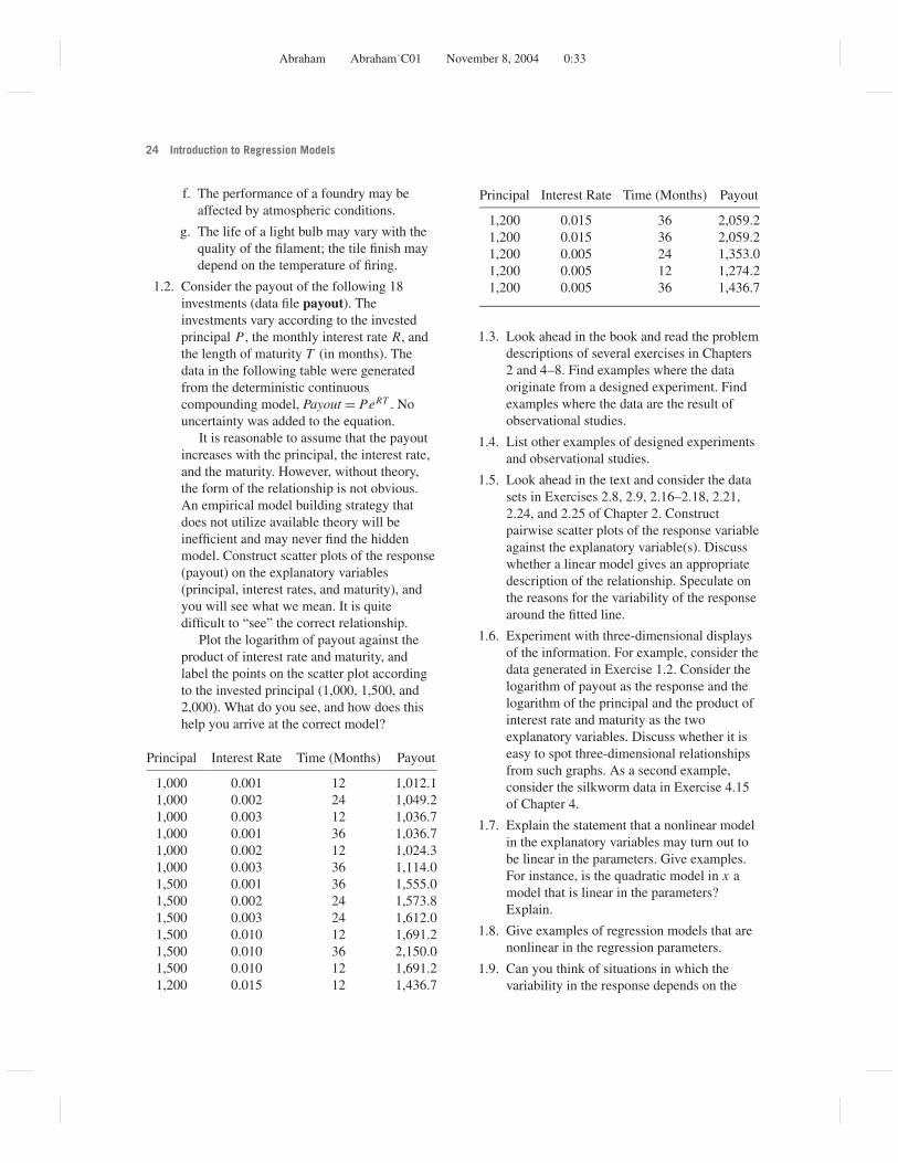
1.2. Consider the payout of the following 18investments (data file payout). Theinvestments vary according to the investedprincipal P , the monthly interest rate R, andthe length of maturity T (in months). Thedata in the following table were generatedfrom the deterministic continuouscompounding model, Payout = PeRT . Nouncertainty was added to the equation.

It is reasonable to assume that the payoutincreases with the principal, the interest rate,and the maturity. However, without theory,the form of the relationship is not obvious.An empirical model building strategy thatdoes not utilize available theory will beinefficient and may never find the hiddenmodel. Construct scatter plots of the response(payout) on the explanatory variables(principal, interest rates, and maturity), andyou will see what we mean. It is quitedifficult to “see” the correct relationship.

Plot the logarithm of payout against theproduct of interest rate and maturity, andlabel the points on the scatter plot accordingto the invested principal (1,000, 1,500, and2,000). What do you see, and how does thishelp you arrive at the correct model?

Principal Interest Rate Time (Months) Payout

1,000 0.001 12 1,012.11,000 0.002 24 1,049.21,000 0.003 12 1,036.71,000 0.001 36 1,036.71,000 0.002 12 1,024.31,000 0.003 36 1,114.01,500 0.001 36 1,555.01,500 0.002 24 1,573.81,500 0.003 24 1,612.01,500 0.010 12 1,691.21,500 0.010 36 2,150.01,500 0.010 12 1,691.21,200 0.015 12 1,436.7

Principal Interest Rate Time (Months) Payout

1,200 0.015 36 2,059.21,200 0.015 36 2,059.21,200 0.005 24 1,353.01,200 0.005 12 1,274.21,200 0.005 36 1,436.7

1.3. Look ahead in the book and read the problemdescriptions of several exercises in Chapters2 and 4–8. Find examples where the dataoriginate from a designed experiment. Findexamples where the data are the result ofobservational studies.

1.4. List other examples of designed experimentsand observational studies.

1.5. Look ahead in the text and consider the datasets in Exercises 2.8, 2.9, 2.16–2.18, 2.21,2.24, and 2.25 of Chapter 2. Constructpairwise scatter plots of the response variableagainst the explanatory variable(s). Discusswhether a linear model gives an appropriatedescription of the relationship. Speculate onthe reasons for the variability of the responsearound the fitted line.

1.6. Experiment with three-dimensional displaysof the information. For example, consider thedata generated in Exercise 1.2. Consider thelogarithm of payout as the response and thelogarithm of the principal and the product ofinterest rate and maturity as the twoexplanatory variables. Discuss whether it iseasy to spot three-dimensional relationshipsfrom such graphs. As a second example,consider the silkworm data in Exercise 4.15of Chapter 4.

1.7. Explain the statement that a nonlinear modelin the explanatory variables may turn out tobe linear in the parameters. Give examples.For instance, is the quadratic model in x amodel that is linear in the parameters?Explain.

1.8. Give examples of regression models that arenonlinear in the regression parameters.

1.9. Can you think of situations in which thevariability in the response depends on the


Exercises 25

level of the explanatory variables? Forexample, consider sales that increase overtime. Why is it reasonable to expect morevariability in sales when the sales are high?Discuss.

1.10. Causality and correlation. Assume that acertain data set exhibits a strong associationamong two variables. Does this imply thatthere is a causal link? Can you think ofexamples where two variables are correlatedbut not causally related? What about theannual number of storks and the annualnumber of human births? Assume that yourdata come from a time period of increasingprosperity, such as the one immediatelyfollowing World War II. Prosperity mayimpact the storks, and it may also affectcouples’ decisions to have families. Hence,you may see a strong (positive) correlationbetween the number of storks and the numberof human births. However, you know thatthere is no causal effect. Can you describe theunderlying principle of this example? Giveother examples?

1.11. Collect the following information. Obtainaverage test scores for the elementary schoolsin your state (region). Obtain data on theproportion of children on subsidized lunch.Construct scatter plots. Do you think thatthere is a causal link between test scores andthe proportion of children on subsidizedlunch? If not, how do you explain the resultsyou see. What if you had data on averageincome or the educational level of parentsin these districts? Do you expect similarresults?

1.12. Salary raises are usually expressed inpercentage terms. This means that two peoplewith the same percentage raise, but differentprevious salaries, will get different monetary(dollar) raises. Assume that the relative raise(R = RelativeRaise = PercentageRaise/100)

is strictly proportional to performance (thatis, RelativeRaise = βPerformance).a. A plot of RelativeRaise againstPerformance exhibits a perfect linearrelationship through the origin. Would a plotof AbsoluteRaise against Performance alsoexhibit a perfect linear association? Would aregression of AbsoluteRaise againstPerformance lead to the desired slopeparameter β?b. Consider the logarithmic transformation ofthe ratio (CurrentSalary/ PreviousSalary).What if you were to plot the logarithm of thisratio against the performance? How wouldthis help you?

1.13. Consider Example 1.2.6 in which we studiedthe effectiveness of five oral contraceptives.We used model (1.8),

yi = αzi + β1xi1 + · · · + β5xi5 + εi

where zi and yi are the HDLC readings at thebeginning and after 6 months, and x1, . . . , x5

are indicators for the five treatment(contraceptive) groups.

How would you convince someone thatthis is an appropriate specification? In orderto address this question, you may want tolook at five separate scatter plots of y againstz, one for each contraceptive group. Makesure these graphs are made with identicalscales on both axes. Have the statisticalsoftware of your choice draw in the “bestfitting” straight lines. Your model in Eq. (1.8)puts certain requirements on the slopes ofthese five graphs. What are theserequirements?

How would you explain a model in whichα = 1? In this case, the emphasis is onchanges in the HDLC, and the questionbecomes whether the magnitudes of thechanges are related to the contraceptives.How would you analyze the data under thisscenario?

Documents

COPYRIGHT Abraham, B. and Ledolter, J. …statmath.wu-wien.ac.at/~ledolter/AbrahamLedolterRegressionChapter1.pdfon a line with slope one and intercept log(P). ... periods are plotted