Embed Size (px)
Citation preview

Copyright 2015 Jingwei Zhu
EXPERIMENTAL INVESTIGATION OF VORTEX TUBE AND VORTEX NOZZLE FOR
APPLICATIONS IN AIR-CONDITIONING, REFRIGERATION, AND HEAT PUMP SYSTEMS
BY
JINGWEI ZHU
THESIS
Submitted in partial fulfillment of the requirements for the degree of Master of Science in Mechanical Engineering
in the Graduate College of the University of Illinois at Urbana-Champaign, 2015
Urbana, Illinois
Adviser:
Professor Stefan Elbel
ii
ABSTRACT
The Ranque-Hilsch vortex tube can separate an incoming high pressure fluid stream into
two low pressure fluid streams with different temperatures. In this project, the applicability of
expansion work recovery through vortex tube in heating and cooling cycles has been examined.
Vortex tube thermal separation performance for air, R134a and carbon dioxide is provided. It has
been found that when using single-phase vapor as the working fluid the vortex tube cold end
temperature can always be lower than the isenthalpic expansion temperature, and whether the hot
end temperature is higher than the inlet temperature depends on whether the fluid shows ideal
gas behavior. Suitable vortex tube operating conditions are identified. Vortex tube cold-side
isentropic efficiencies are measured to be higher than 20% for different fluids. Based on this
knowledge, cooling and heating cycles with vortex tube have been proposed and their
performance is calculated.
Expansion work recovery by two-phase ejector is known to be beneficial to vapor
compression cycle performance. However, one of the biggest challenges with ejector vapor
compression cycle is that the ejector cycle performance is sensitive to working condition changes
which are common in real world applications. Different working conditions require different
ejector geometries to achieve maximum performance. Slightly different geometries may result in
substantially different COPs under the same conditions. The ejector motive nozzle throat
diameter (motive nozzle restrictiveness) is one of the key parameters that can significantly affect
COP. This thesis presents a new two-phase nozzle restrictiveness control mechanism which is
possibly applicable to two-phase ejectors used in vapor compression cycles. This new control
mechanism has the advantages of being simple and potentially less costly. It can also possibly
avoid the additional frictional losses of previously proposed ejector control mechanisms using
adjustable needle. An adjustable nozzle based on this new control mechanism is designed and
manufactured for experiments with R134a. The experimental results show that, without changing
the nozzle geometry, the nozzle restrictiveness on the two-phase flow can be adjusted over a
wide range. Under the same inlet and outlet conditions, the mass flow rate through the nozzle can
be reduced by 36% of the full load. This feature could be very useful for the future application of
ejectors in mobile or stationary systems under changing working conditions.

iii
To my father and mother, for their support, sacrifice and understanding.
iv
ACKNOWLEDGMENTS
This project would not have been possible without the support of many people. I would
like to express my deepest gratitude to Professor Stefan Elbel and Professor Predrag Stojan
Hrnjak for their help, guidance, and encouragement. The training I have received from them on
how to conduct research and how to generate creative but realistic solutions to real world
problems is one of the most valuable assets in my life. I would also like to thank Mr. Neal D.
Lawrence and Mr. Muhammad Reaz Mohiuddin for their excellent comments, insightful
suggestions and patient help with my experimentation. Special thanks to the member companies
of the Air Conditioning and Refrigeration Center at the University of Illinois at Urbana-
Champaign for their generous support of this project. Finally, I would like to thank all my family,
friends, and colleagues for their help, encouragement and wisdom.
v
TABLE OF CONTENTS
LIST OF FIGURES ...................................................................................................................VII
LIST OF TABLES ........................................................................................................................X
CHAPTER 1: INTRODUCTION................................................................................................ 1
1.1 BACKGROUND AND MOTIVATION...................................................................................... 1 1.2 OBJECTIVE OF RESEARCH.................................................................................................. 2 1.3 STRUCTURE OF THESIS ...................................................................................................... 3 1.4 PUBLICATIONS FROM THE PROJECT................................................................................... 4
CHAPTER 2: VORTEX TUBE BACKGROUND AND LITERATURE REVIEW.............. 5
2.1 NOMENCLATURE ............................................................................................................... 5 2.2 VORTEX TUBE FUNDAMENTALS........................................................................................ 6 2.3 PREVIOUS EXPERIMENTAL AND NUMERICAL INVESTIGATION OF VORTEX TUBE .............. 8 2.4 VORTEX TUBE APPLICATIONS IN REFRIGERATION AND AIR-CONDITIONING FOR
EXPANSION WORK RECOVERY APPLICATIONS ........................................................................... 10 2.5 SUMMARY OF LITERATURE REVIEW................................................................................ 11
CHAPTER 3: EXPERIMENTAL FACILITY AND METHODS FOR INVESTIGATION
OF VORTEX TUBE THERMAL SEPARATION .................................................................. 13
3.1 COMMERCIAL COUNTER-FLOW VORTEX TUBE DESIGN .................................................. 13 3.2 IMPROVED COUNTER-FLOW VORTEX TUBE DESIGN ....................................................... 13 3.3 EXPERIMENTAL SETUP AND ITS COMPONENTS ................................................................ 16 3.4 TEST METHODS AND CONDITIONS................................................................................... 19 3.5 EXPERIMENTAL UNCERTAINTIES..................................................................................... 20
CHAPTER 4: EXPERIMENTAL INVESTIGATION OF VORTEX TUBE THERMAL
SEPARATION ............................................................................................................................ 22
4.1 EXPERIMENTAL RESULTS WITH AIR ................................................................................ 22 4.2 EXPERIMENTAL RESULTS WITH R134A ........................................................................... 25 4.3 EXPERIMENTAL RESULTS WITH CARBON DIOXIDE .......................................................... 30
CHAPTER 5: NUMERICAL ANALYSIS OF POSSIBLE VORTEX TUBE CYCLES FOR
COOLING AND HEATING...................................................................................................... 33
5.1 VORTEX TUBE COOLING CYCLE...................................................................................... 34 5.2 VORTEX TUBE HEATING CYCLE...................................................................................... 36 5.3 SUMMARY OF NUMERICAL ANALYSIS OF VORTEX TUBE CYCLES ................................... 45
CHAPTER 6: EJECTOR BACKGROUND AND LITERATURE REVIEW...................... 47
6.1 NOMENCLATURE ............................................................................................................. 47 6.2 EJECTOR FUNDAMENTALS............................................................................................... 47
vi
6.3 EJECTOR FOR EXPANSION WORK RECOVERY IN VAPOR COMPRESSION CYCLES............. 48 6.4 INFLUENCE OF WORKING CONDITIONS AND EJECTOR DIMENSIONS ON EJECTOR CYCLE
PERFORMANCE ........................................................................................................................... 51 6.5 SUMMARY OF LITERATURE REVIEW................................................................................ 53
CHAPTER 7: NEW VORTEX CONTROL POSSIBLY APPLICABLE TO EJECTOR
REFRIGERATION CYCLES ................................................................................................... 54
7.1 INTRODUCTION TO VORTEX EJECTOR AND VORTEX CONTROL ....................................... 54 7.2 HYPOTHESIS FOR THE INFLUENCE OF NOZZLE INLET VORTEX ON THE TWO-PHASE
NOZZLE RESTRICTIVENESS......................................................................................................... 56
CHAPTER 8: EXPERIMENTAL FACILITY AND METHODS FOR INVESTIGATION
OF THE INFLUENCE OF INLET VORTEX ON NOZZLE RESTRICTIVENESS.......... 58
8.1 VORTEX NOZZLE DESIGN................................................................................................ 58 8.2 EXPERIMENTAL SETUP AND ITS COMPONENTS ................................................................ 60 8.3 TEST METHODS AND CONDITIONS................................................................................... 62 8.4 EXPERIMENTAL UNCERTAINTIES..................................................................................... 63
CHAPTER 9: VORTEX NOZZLE TESTS WITH REFRIGERANT (R134A) ................... 64
CHAPTER 10: CONCLUSIONS AND FUTURE WORK ..................................................... 69
REFERENCES............................................................................................................................ 71
APPENDIX A: DETAILS OF EXPERIMENTAL FACILITY ............................................. 75
A.1 REFRIGERANT PUMP........................................................................................................ 75 A.2 WATER HEATER .............................................................................................................. 75 A.3 REFRIGERANT HEATER/EVAPORATOR............................................................................. 76 A.4 CONDENSER AND SUBCOOLER......................................................................................... 77
A.5 RANGES AND ACCURACIES OF SENSORS.......................................................................... 78
APPENDIX B: ADDITIONAL VORTEX TUBE COMPONENT DRAWINGS ................. 84
APPENDIX C: RAW EXPERIMENTAL DATA .................................................................... 90
vii
LIST OF FIGURES
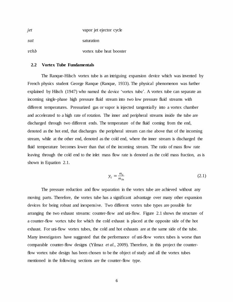
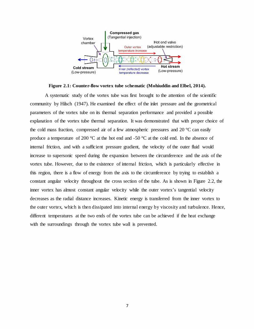
Figure 2.1: Counter-flow vortex tube schematic (Mohiuddin and Elbel, 2014). ............................ 7
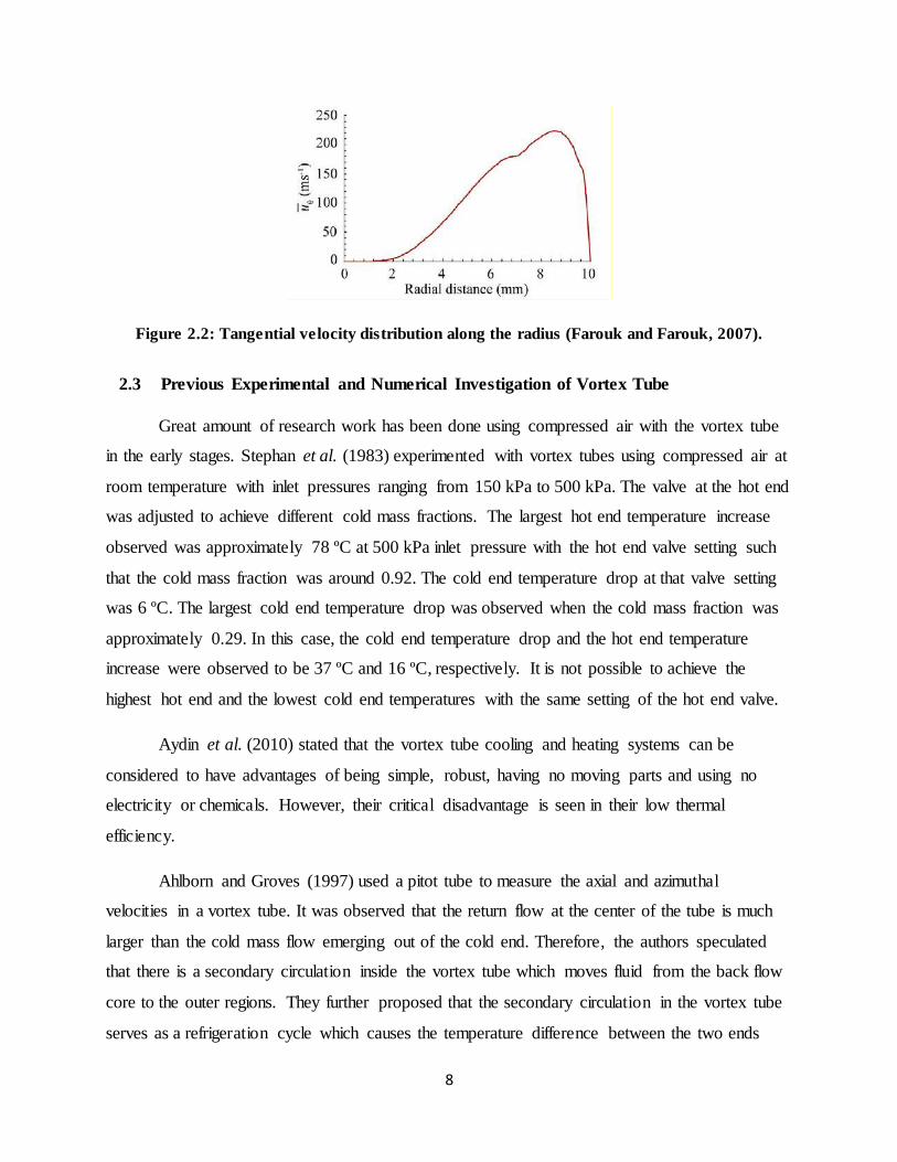
Figure 2.2: Tangential velocity distribution along the radius (Farouk and Farouk, 2007). ............ 8
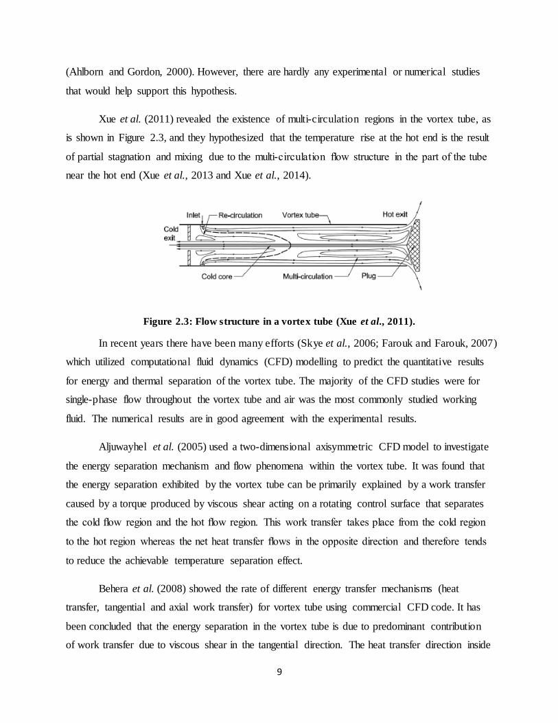
Figure 2.3: Flow structure in a vortex tube (Xue et al., 2011). ...................................................... 9
Figure 3.1: Commercially available counter-flow vortex tube with its components (Mohiuddin
and Elbel, 2014). ........................................................................................................................... 13
Figure 3.2: Improved counter- flow vortex tube with modified hot end valve. ............................. 14
Figure 3.3: Drawing of the vortex generator. ................................................................................ 14
Figure 3.4: Drawing of the tube body. .......................................................................................... 15
Figure 3.5: Assembly drawing of the improved counter- flow vortex tube................................... 15
Figure 3.6: Experimental setup for air tests. ................................................................................. 17
Figure 3.7: Closed system experimental setup for vortex tube performance tests with refrigerants
(Mohiuddin and Elbel, 2014). ....................................................................................................... 18
Figure 3.8: Laboratory facility for vortex tube performance tests with refrigerants (Mohiuddin
and Elbel, 2014). ........................................................................................................................... 19
Figure 4.1: Cold and hot end temperature distribution when using air. ....................................... 23
Figure 4.2: Vortex tube cold-side isentropic efficiency and cold end temperature distribution at
different cold mass fractions compared to inlet, isenthalpic and isentropic expansion
temperatures when using air. ........................................................................................................ 24
Figure 4.3: Pressure-specific enthalpy plot showing the inlet and outlets of the vortex tube when
the lowest cold end temperature or the highest hot end temperature is reached using air. ........... 25
Figure 4.4: Distribution of temperatures at the cold and hot ends when using R134a with
Pin=1121 kPa. ............................................................................................................................... 26
Figure 4.5: Distribution of temperatures at the cold and hot ends when using R134a with
Pin=1023 kPa. ............................................................................................................................... 26
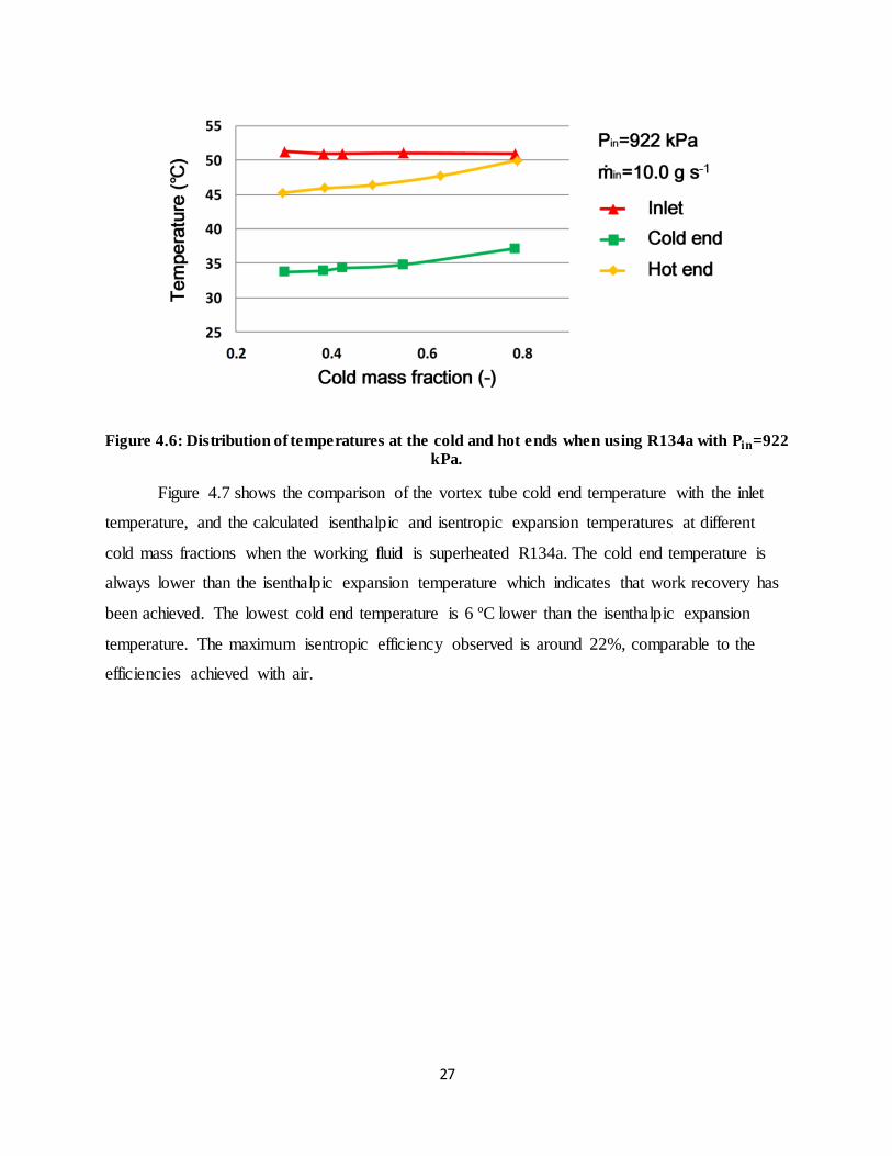
Figure 4.6: Distribution of temperatures at the cold and hot ends when using R134a with
Pin=922 kPa. ................................................................................................................................. 27
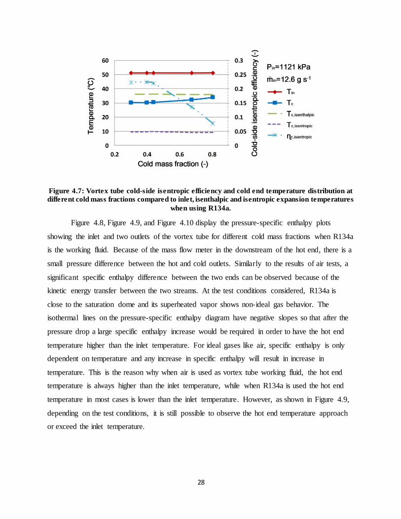
Figure 4.7: Vortex tube cold-side isentropic efficiency and cold end temperature distribution at
different cold mass fractions compared to inlet, isenthalpic and isentropic expansion
temperatures when using R134a. .................................................................................................. 28
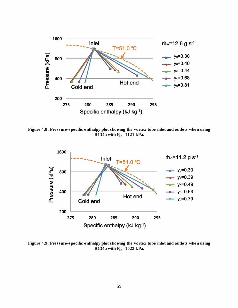
Figure 4.8: Pressure-specific enthalpy plot showing the vortex tube inlet and outlets when using
R134a with Pin=1121 kPa. ........................................................................................................... 29
Figure 4.9: Pressure-specific enthalpy plot showing the vortex tube inlet and outlets when using
R134a with Pin=1023 kPa. ........................................................................................................... 29
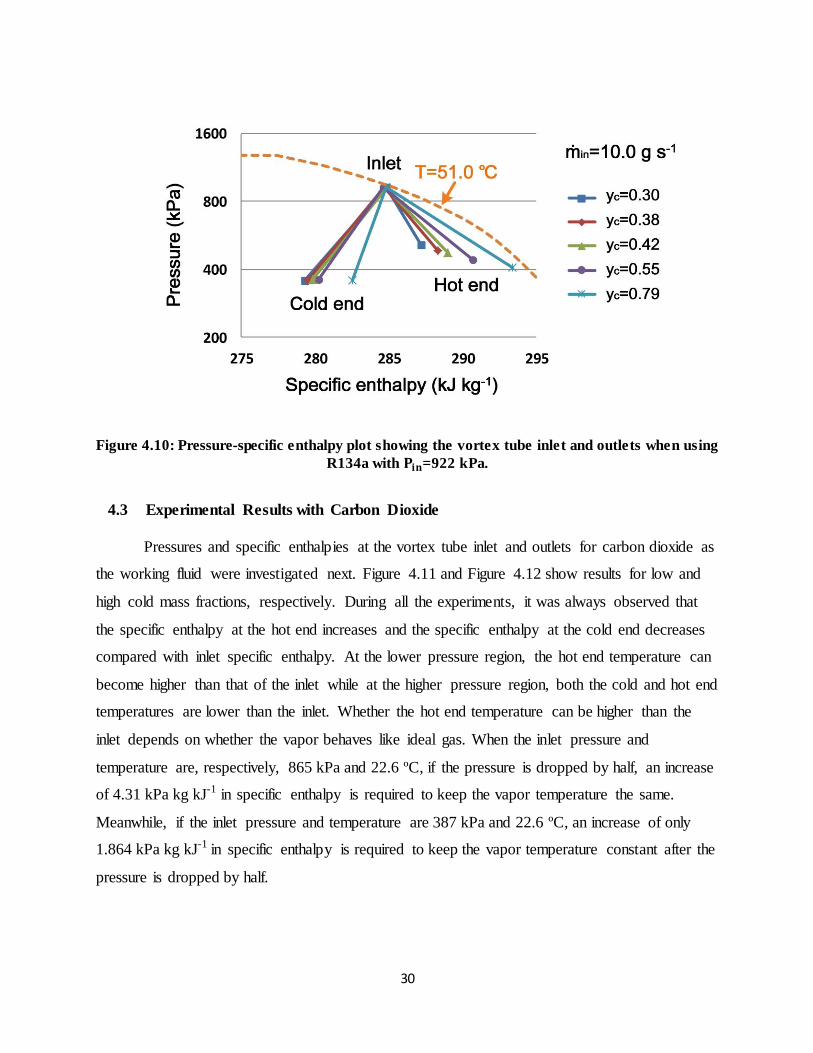
Figure 4.10: Pressure-specific enthalpy plot showing the vortex tube inlet and outlets when using
R134a with Pin=922 kPa. ............................................................................................................. 30
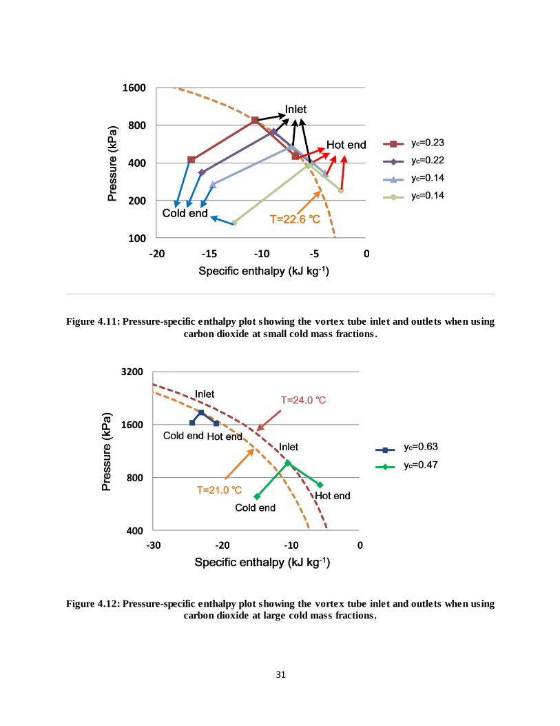
Figure 4.11: Pressure-specific enthalpy plot showing the vortex tube inlet and outlets when using
carbon dioxide at small cold mass fractions. ................................................................................ 31
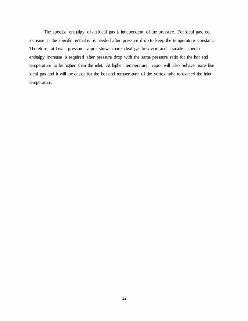
Figure 4.12: Pressure-specific enthalpy plot showing the vortex tube inlet and outlets when using
carbon dioxide at large cold mass fractions. ................................................................................. 31
viii
Figure 5.1: Schematic of vapor compression cooling cycle with vortex tube. ............................. 35
Figure 5.2: Thermodynamic state point diagram of vapor compression cooling cycle with vortex
tube................................................................................................................................................ 35
Figure 5.3: Schematic of heat booster cycle with vortex tube. ..................................................... 37
Figure 5.4: Thermodynamic state point diagram of heat booster cycle with vortex tube. ........... 37
Figure 5.5: Calculated COP for vortex tube heat booster using R134a at different vortex tube
cold-side isentropic efficiencies and high side pressures. ............................................................ 38
Figure 5.6: Calculated COP for vortex tube heat booster using R245fa at different vortex tube
cold-side isentropic efficiencies and high side pressures. ............................................................ 39
Figure 5.7: Calculated COP for vortex tube heat booster using R141b at different vortex tube
cold-side isentropic efficiencies and high side pressures. ............................................................ 39
Figure 5.8: Heat driven cooling cycle using ejector with vortex tube heat booster...................... 40
Figure 5.9: Entrainment ratio of vapor jet ejector cooling cycle using R245fa for different ejector
motive flow superheats. ................................................................................................................ 41
Figure 5.10: Entrainment ratio of vapor jet ejector cooling cycle using water for different ejector
motive flow superheats. ................................................................................................................ 42
Figure 5.11: Entrainment ratio of vapor jet ejector cooling cycle using R245fa with different
ejector motive flow superheats at critical operating conditions. ................................................... 43
Figure 5.12: Influence of vortex tube cold side isentropic efficiency on maximum overall COP of
vapor jet ejector cooling cycle with vortex tube heat booster using R245fa in both cycles. ........ 44
Figure 5.13: Maximum overall COP with superheat provided by vortex tube heat booster using
R245fa under critical conditions. .................................................................................................. 45
Figure 6.1: Diagram of a typical ejector. ...................................................................................... 48
Figure 6.2: Layout of the two-phase ejector cycle as proposed by Gay (1931). .......................... 49
Figure 6.3: Pressure-specific enthalpy diagram of the two-phase ejector cycle as proposed by
Gay (1931). ................................................................................................................................... 49
Figure 6.4: Variable ejector with adjustable needle in the motive nozzle. ................................... 52
Figure 7.1: (a) Conventional ejector and (b) vortex ejector. ......................................................... 55
Figure 7.2: Vortex ejector cooling cycle....................................................................................... 55
Figure 7.3: Two approaches to increase two-phase nozzle restrictiveness: (a) changing nozzle
geometry; (b) increasing vapor generation by applying inlet vortex without changing nozzle
geometry........................................................................................................................................ 57
Figure 8.1: Vortex nozzle composed of tee, sleeve and convergent-divergent nozzle. ................ 58
Figure 8.2: 3D printed transparent convergent-divergent nozzle. ................................................ 59
Figure 8.3: Experimental facility for investigation of vortex influence on nozzle restrictiveness.
....................................................................................................................................................... 61
Figure 9.1: Effect of vortex nozzle outlet pressure on the vortex nozzle total mass flow rate for
different constant inlet pressures. .................................................................................................. 65
ix
Figure 9.2: Flow expanded in the convergent-divergent nozzle: (a) choked flow (Pin = 921
kPa, Pout = 419 kPa, Tin = 36.2 ºC); (b) nozzle outlet pressure close to the inlet pressure (Pin =
930 kPa, Pout = 885 kPa, Tin = 35.9 ºC). .................................................................................... 66
Figure 9.3: Influence of nozzle inlet vortex strength on the total mass flow rate through the
nozzle at different constant inlet conditions (all data points for choked flow). ............................ 67
Figure 9.4: Nozzle inlet pressure variations for different inlet vortex strengths at constant total
mass flow rates (all data points for choked flow). ........................................................................ 68
Figure A.1: Reciprocating piston pump for circulating liquid refrigerant. ................................... 75
Figure A.2: Water heater and submersible water pump. .............................................................. 76
Figure A.3: Plate heat exchanger used as heater/evaporator in vortex nozzle and vortex tube tests.
....................................................................................................................................................... 77
Figure A.4: Plate heat exchanger used as condenser/subcooler. .................................................. 78
Figure B.1: Vortex tube component 1 (sleeve). ............................................................................ 84
Figure B.2: Vortex tube component 2 (cold end body). ............................................................... 85
Figure B.3: Vortex tube component 5 (washer). ........................................................................... 86
Figure B.4: Vortex tube component 6 (plug). ............................................................................... 87
Figure B.5: Vortex tube component 7 (hot end valve). ................................................................ 88
Figure B.6: Vortex tube component 8 (hot end valve body). ....................................................... 89
x
LIST OF TABLES
Table 3.1: Vortex tube geometric parameters. .............................................................................. 16
Table 3.2: Vortex tube test matrix. ............................................................................................... 20
Table 3.3: Experimental uncertainties of variables in the vortex tube experiments. .................... 21
Table 8.1: Vortex nozzle geometric parameters. .......................................................................... 59
Table 8.2: Vortex nozzle test matrix. ............................................................................................ 63
Table 8.3: Experimental uncertainties of variables in the vortex nozzle experiments. ................ 63
Table A.1: Summary of ranges and accuracies of sensors used for vortex tube thermal separation
performance tests with air. ............................................................................................................ 78
Table A.2: Summary of ranges and accuracies of sensors used for vortex tube thermal separation
performance tests with R134a....................................................................................................... 79
Table A.3: Summary of ranges and accuracies of sensors used for vortex tube thermal separation
performance tests with carbon dioxide. ........................................................................................ 81
Table A.4: Summary of ranges and accuracies of sensors used for vortex nozzle tests with R134a.
....................................................................................................................................................... 82
Table C.1: Experimental raw data from the performance tests of vortex tube with air at 670 kPa
vortex tube inlet pressure, 24 ºC vortex tube inlet temperature, 100 kPa cold end and hot end
pressures........................................................................................................................................ 90
Table C.2: Experimental raw data from the performance tests of vortex tube with R134a. ........ 92
Table C.3: Experimental raw data from the performance tests of vortex tube with carbon dioxide.
....................................................................................................................................................... 95
Table C.4: Experimental raw data from the vortex nozzle tests with R134a. .............................. 97
1
CHAPTER 1: INTRODUCTION
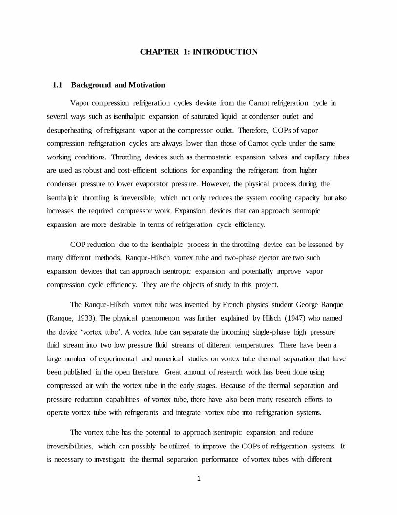
1.1 Background and Motivation
Vapor compression refrigeration cycles deviate from the Carnot refrigeration cycle in
several ways such as isenthalpic expansion of saturated liquid at condenser outlet and
desuperheating of refrigerant vapor at the compressor outlet. Therefore, COPs of vapor
compression refrigeration cycles are always lower than those of Carnot cycle under the same
working conditions. Throttling devices such as thermostatic expansion valves and capillary tubes
are used as robust and cost-efficient solutions for expanding the refrigerant from higher
condenser pressure to lower evaporator pressure. However, the physical process during the
isenthalpic throttling is irreversible, which not only reduces the system cooling capacity but also
increases the required compressor work. Expansion devices that can approach isentropic
expansion are more desirable in terms of refrigeration cycle efficiency.
COP reduction due to the isenthalpic process in the throttling device can be lessened by
many different methods. Ranque-Hilsch vortex tube and two-phase ejector are two such
expansion devices that can approach isentropic expansion and potentially improve vapor
compression cycle efficiency. They are the objects of study in this project.
The Ranque-Hilsch vortex tube was invented by French physics student George Ranque
(Ranque, 1933). The physical phenomenon was further explained by Hilsch (1947) who named
the device ‘vortex tube’. A vortex tube can separate the incoming single-phase high pressure
fluid stream into two low pressure fluid streams of different temperatures. There have been a
large number of experimental and numerical studies on vortex tube thermal separation that have
been published in the open literature. Great amount of research work has been done using
compressed air with the vortex tube in the early stages. Because of the thermal separation and
pressure reduction capabilities of vortex tube, there have also been many research efforts to
operate vortex tube with refrigerants and integrate vortex tube into refrigeration systems.
The vortex tube has the potential to approach isentropic expansion and reduce
irreversibilities, which can possibly be utilized to improve the COPs of refrigeration systems. It
is necessary to investigate the thermal separation performance of vortex tubes with different
2
refrigerants. Based on the experimental investigation of vortex tube thermal separation
performance with refrigerants, realistic vortex tube refrigeration cycles can be proposed and the
overall gain in the system COP and capacity by the introduction of vortex tubes can be
numerically evaluated. Meanwhile, other possible applications of vortex tube utilizing the
heating feature of vortex tube are also worth exploring.
Expansion devices that involve expansion work recovery are known to be more beneficial
in terms of cycle efficiency and cooling capacity. The ejector is one of the expansion work
recovery devices that receive most attention in research studies. Ejector refrigeration cycles
utilize the kinetic energy released during the pressure reduction of the fluid as it passes from the
high to the low-pressure side to entrain and compress the fluid from the evaporator, thus the
compressor work is saved. The ejector can also be utilized to overfeed the evaporator so that
better heat exchanger performance is achieved, and thus the cycle cooling capacity and the COP
can both be improved.
Ejector cycle performance is usually sensitive to working condition changes. It is
desirable to introduce an adjustable feature to the ejector so that ejector cycle performance can
be optimized under different working conditions, which could make ejector technology more
suitable for real world applications. The ejector motive nozzle throat diameter (motive nozzle
restrictiveness) is one of the key dimensions that affect COP. It has a direct impact on motive
mass flow rate. Previous adjustable ejector designs with variable motive nozzle throat diameter
are complicated and costly, and have lower nozzle and ejector efficiencies compared with
conventional ejector. This provides motivation to develop a new technology to control the
motive nozzle restrictiveness.
1.2 Objective of Research
In the previous studies of vortex tube refrigeration cycles, very optimistic assumptions
have been made for the cycle analysis. To achieve a more realistic evaluation of vortex tube
refrigeration cycle performance, it is important to conduct experimental investigation of vortex
tubes with refrigerants. Based on the experimental results, realistic vortex tube refrigeration
cycles can be proposed and the overall gain in the system COP and capacity can be numerically
3
analyzed. Meanwhile, applications of other features of the vortex tube such as heating can also
be explored.
A novel control mechanism to adjust the two-phase nozzle restrictiveness which is
possibly applicable to the control of ejector cooling cycles has been presented in this thesis. It
utilizes an adjustable vortex at the nozzle inlet to control the nozzle restrictiveness on the low
vapor quality flow expanded in the nozzle without changing the physical dimensions of the
nozzle geometry. The controllability of nozzle restrictiveness with this new control mechanism
needs to be shown in order to evaluate its usefulness in real world applications.
The objectives of this thesis are as follows:
Experimentally investigate the thermal separation performance of vortex tube with air,
R134a and carbon dioxide in superheated vapor state.
Explore novel vortex tube cycles to increase the capacity and COP of vapor compression
refrigerating systems.
Explore novel cycles to utilize the heating feature of vortex tube through numerical
analysis.
Experimentally investigate the influence of nozzle inlet vortex on the nozzle
restrictiveness on the two-phase flow.
Explain the influence of nozzle inlet vortex on the two-phase nozzle restrictiveness.
Visualize the low-quality swirling flow expanded in the nozzle.
1.3 Structure of Thesis
Chapter 1 of this thesis has presented some motivation for and the objectives of the work
done in this study on vortex tube and vortex nozzle.
Chapter 2 presents more detailed information about the working principles of vortex tube,
previous experimental and numerical investigations of vortex tube thermal separation and studies
on the applications of vortex tube in refrigerating systems. Chapter 3 describes the experimental
facility and methods used to investigate the vortex tube thermal separation performance with
different working fluids. Chapter 4 presents the vortex tube experimental results with working
fluids including air, R134a and carbon dioxide. Chapter 5 numerically analyzes several vortex
4
tube cycles for cooling and heating. Realistic vortex tube performance and working conditions
based on the previous experimental results have been assumed in the numerical analysis.
Chapter 6 presents an overview of the operation of ejector as well as a literature review of
the use of two-phase ejector in both subcritical and transcritical refrigerating systems. The
literature review shows the improvement to vapor compression cycle performance brought by the
introduction of ejector and the importance of introducing adjustable geometry feature to ejector
refrigerating cycles. Chapter 7 presents a new control mechanism for the restrictiveness of a two-
phase nozzle, vortex control, which can possibly be applied to the control of ejector cooling
cycles. A hypothesis has been provided for the influence of nozzle inlet vortex on the two-phase
nozzle restrictiveness. Chapter 8 describes the experimental facility and methods used to
investigate the inlet vortex influence on the two-phase nozzle restrictiveness. Chapter 9 presents
and discusses the vortex nozzle experimental results as well as preliminary visualization results
with R134a as the working fluid.
Finally, Chapter 10 summarizes the conclusions that can be drawn from this work and
provides possible directions for future work.
1.4 Publications from The Project
Zhu, J., Mohiuddin, M., Elbel, S., 2014. Vortex tubes used as expansion device in vapor
compression systems. 11th IIR Gustav Lorentzen Conference on Natural Refrigerants: Natural
Refrigerants and Environmental Protection, Hangzhou, China, Paper 43.
Zhu, J., Elbel, S., 2015. Vortex tube heat booster to improve performance of heat driven cooling
cycles. 24th IIR International Congress of Refrigeration, Yokohama, Japan, Paper 299.
Zhu, J., Elbel, S., 2015. Fresh look at vortex tubes and their potential use as expansion device in
automotive vapor compression systems. Presented at SAE 2015 Thermal Management Systems
Symposium, Troy, MI, USA.
5
CHAPTER 2: VORTEX TUBE BACKGROUND AND LITERATURE REVIEW
2.1 Nomenclature
Symbols
𝐶𝑚 simulation correction factor [-]
𝐶𝑂𝑃 coefficient of performance [-]
ℎ specific enthalpy [kJ kg-1]
�̇� mass flow rate [g s-1]
𝑃 pressure [kPa]
𝑄 heating/cooling capacity [kW]
𝑇 temperature [ºC]
𝑊 power [kW]
𝑦 mass fraction [-]
Greek Symbols
𝜂 efficiency [-]
Subscripts
𝑐 cold end
evap evaporator
ℎ hot end
𝑖𝑛 inlet
𝑖𝑠𝑒𝑛𝑡𝑟𝑜𝑝𝑖𝑐 isentropic process
6
jet vapor jet ejector cycle
𝑠𝑎𝑡 saturation
𝑣𝑡ℎ𝑏 vortex tube heat booster
2.2 Vortex Tube Fundamentals
The Ranque-Hilsch vortex tube is an intriguing expansion device which was invented by
French physics student George Ranque (Ranque, 1933). The physical phenomenon was further
explained by Hilsch (1947) who named the device ‘vortex tube’. A vortex tube can separate an
incoming single-phase high pressure fluid stream into two low pressure fluid streams with
different temperatures. Pressurized gas or vapor is injected tangentially into a vortex chamber
and accelerated to a high rate of rotation. The inner and peripheral streams inside the tube are
discharged through two different ends. The temperature of the fluid coming from the end,
denoted as the hot end, that discharges the peripheral stream can rise above that of the incoming
stream, while at the other end, denoted as the cold end, where the inner stream is discharged the
fluid temperature becomes lower than that of the incoming stream. The ratio of mass flow rate
leaving through the cold end to the inlet mass flow rate is denoted as the cold mass fraction, as is
shown in Equation 2.1.
𝑦𝑐 =�̇�𝑐
�̇�𝑖𝑛 (2.1)
The pressure reduction and flow separation in the vortex tube are achieved without any
moving parts. Therefore, the vortex tube has a significant advantage over many other expansion
devices for being robust and inexpensive. Two different vortex tube types are possible for
arranging the two exhaust streams: counter-flow and uni-flow. Figure 2.1 shows the structure of
a counter-flow vortex tube for which the cold exhaust is placed at the opposite side of the hot
exhaust. For uni-flow vortex tubes, the cold and hot exhausts are at the same side of the tube.
Many investigators have suggested that the performance of uni-flow vortex tubes is worse than
comparable counter-flow designs (Yilmaz et al., 2009). Therefore, in this project the counter-
flow vortex tube design has been chosen to be the object of study and all the vortex tubes
mentioned in the following sections are the counter-flow type.
7
Figure 2.1: Counter-flow vortex tube schematic (Mohiuddin and Elbel, 2014).
A systematic study of the vortex tube was first brought to the attention of the scientific
community by Hilsch (1947). He examined the effect of the inlet pressure and the geometrical
parameters of the vortex tube on its thermal separation performance and provided a possible
explanation of the vortex tube thermal separation. It was demonstrated that with proper choice of
the cold mass fraction, compressed air of a few atmospheric pressures and 20 °C can easily
produce a temperature of 200 °C at the hot end and -50 °C at the cold end. In the absence of
internal friction, and with a sufficient pressure gradient, the velocity of the outer fluid would
increase to supersonic speed during the expansion between the circumference and the axis of the
vortex tube. However, due to the existence of internal friction, which is particularly effective in
this region, there is a flow of energy from the axis to the circumference by trying to establish a
constant angular velocity throughout the cross section of the tube. As is shown in Figure 2.2, the
inner vortex has almost constant angular velocity while the outer vortex’s tangential velocity
decreases as the radial distance increases. Kinetic energy is transferred from the inner vortex to
the outer vortex, which is then dissipated into internal energy by viscosity and turbulence. Hence,
different temperatures at the two ends of the vortex tube can be achieved if the heat exchange
with the surroundings through the vortex tube wall is prevented.
8
Figure 2.2: Tangential velocity distribution along the radius (Farouk and Farouk, 2007).
2.3 Previous Experimental and Numerical Investigation of Vortex Tube
Great amount of research work has been done using compressed air with the vortex tube
in the early stages. Stephan et al. (1983) experimented with vortex tubes using compressed air at
room temperature with inlet pressures ranging from 150 kPa to 500 kPa. The valve at the hot end
was adjusted to achieve different cold mass fractions. The largest hot end temperature increase
observed was approximately 78 ºC at 500 kPa inlet pressure with the hot end valve setting such
that the cold mass fraction was around 0.92. The cold end temperature drop at that valve setting
was 6 ºC. The largest cold end temperature drop was observed when the cold mass fraction was
approximately 0.29. In this case, the cold end temperature drop and the hot end temperature
increase were observed to be 37 ºC and 16 ºC, respectively. It is not possible to achieve the
highest hot end and the lowest cold end temperatures with the same setting of the hot end valve.
Aydin et al. (2010) stated that the vortex tube cooling and heating systems can be
considered to have advantages of being simple, robust, having no moving parts and using no
electricity or chemicals. However, their critical disadvantage is seen in their low thermal
efficiency.
Ahlborn and Groves (1997) used a pitot tube to measure the axial and azimuthal
velocities in a vortex tube. It was observed that the return flow at the center of the tube is much
larger than the cold mass flow emerging out of the cold end. Therefore, the authors speculated
that there is a secondary circulation inside the vortex tube which moves fluid from the back flow
core to the outer regions. They further proposed that the secondary circulation in the vortex tube
serves as a refrigeration cycle which causes the temperature difference between the two ends
9
(Ahlborn and Gordon, 2000). However, there are hardly any experimental or numerical studies
that would help support this hypothesis.
Xue et al. (2011) revealed the existence of multi-circulation regions in the vortex tube, as
is shown in Figure 2.3, and they hypothesized that the temperature rise at the hot end is the result
of partial stagnation and mixing due to the multi-circulation flow structure in the part of the tube
near the hot end (Xue et al., 2013 and Xue et al., 2014).
Figure 2.3: Flow structure in a vortex tube (Xue et al., 2011).
In recent years there have been many efforts (Skye et al., 2006; Farouk and Farouk, 2007)
which utilized computational fluid dynamics (CFD) modelling to predict the quantitative results
for energy and thermal separation of the vortex tube. The majority of the CFD studies were for
single-phase flow throughout the vortex tube and air was the most commonly studied working
fluid. The numerical results are in good agreement with the experimental results.
Aljuwayhel et al. (2005) used a two-dimensional axisymmetric CFD model to investigate
the energy separation mechanism and flow phenomena within the vortex tube. It was found that
the energy separation exhibited by the vortex tube can be primarily explained by a work transfer
caused by a torque produced by viscous shear acting on a rotating control surface that separates
the cold flow region and the hot flow region. This work transfer takes place from the cold region
to the hot region whereas the net heat transfer flows in the opposite direction and therefore tends
to reduce the achievable temperature separation effect.
Behera et al. (2008) showed the rate of different energy transfer mechanisms (heat
transfer, tangential and axial work transfer) for vortex tube using commercial CFD code. It has
been concluded that the energy separation in the vortex tube is due to predominant contribution
of work transfer due to viscous shear in the tangential direction. The heat transfer direction inside
10
the vortex tube is generally from the peripheral layers towards the core of the flow .Therefore, a
decrease in heat transfer can result in an increase in net energy transfer. Improperly small cold
outlet diameter selection leads to secondary circulation flow, which has been observed by
Ahlborn and Groves (1997) by experiment, and results in reduced energy transfer.
2.4 Vortex Tube Applications in Refrigeration and Air-Conditioning for Expansion
Work Recovery Applications
Because of the thermal separation and pressure reduction capabilities of vortex tube,
there have been many research efforts to operate vortex tube with refrigerants and integrate
vortex tube into refrigeration systems.
Nellis and Klein (2002) proposed that vortex tube has the potential to improve the
performance of cryogenic refrigeration systems based on the Joule-Thomson cycles and its
derivatives.
Han et al. (2013) experimentally investigated the vortex tube energy separation effects
with different working fluids. For R22, when the vortex tube inlet pressure and temperature are
383 kPa and 12.0 ºC, respectively, the cold end temperature drop is 9.9 ºC, which is greater than
the isenthalpic expansion process temperature drop 7.4 ºC. However, it is much less than the
isentropic expansion process temperature drop 53.0 ºC.
Collins and Lovelace (1979) investigated the temperature separation performance of
vortex tubes with two-phase propane (R290). They observed that the temperature difference
between the hot and cold end of the vortex tube remains significant when the inlet quality is
above about 80%. When the inlet quality drops below 80%, the temperature separation
diminishes to an insignificant level. It was hypothesized that the liquid droplets formed at the
vortex tube inlet are rapidly vaporized at the vortex tube nozzle outlet. As a result, the heating
effect normally occurs in the hot end stream is reduced.
In vapor compression refrigeration cycles, throttling devices such as thermostatic
expansion valves and capillary tubes are used as robust and cost-efficient solutions for expanding
the refrigerant from higher condenser pressure to lower evaporator pressure. However, the
physical process during the isenthalpic throttling is irreversible, which not only reduces the
11
system cooling capacity but also increases the required compressor work. This results in a
decrease in the COP of actual vapor compression refrigeration cycles compared to an ideal
Carnot refrigeration cycle. Fluids such as carbon dioxide which display substantial throttling
losses justify research on expansion devices that can recover expansion work.
Sarkar (2009) numerically analyzed vortex tube expansion transcritical carbon dioxide
refrigeration cycles with two different cycle layouts. However, it has been assumed for the
analysis that all the kinetic energies at the nozzle exit in the vortex tube are absorbed by the hot
flow only, which is very optimistic in reality.
Liu and Jin (2012) proposed and analyzed a transcritical two-stage carbon dioxide
refrigeration cycle using vortex tube expansion. In this cycle, the supercritical fluid from the gas
cooler expands in the vortex tube to the evaporator pressure and is divided into three fractions:
saturated liquid, which is collected in a ring inside the vortex tube, saturated vapor and
superheated gas. The saturated liquid and vapor are mixed again and going through the
evaporator to give useful cooling effect. However, the existence of saturated liquid in the vortex
tube can significantly diminish the temperature separation, as is shown by Collins and
Lovelace’s investigation (1979). Moreover, the extraction of liquid from the vortex tube through
the ring could be highly challenging. No details of the vortex tube design have been provided in
that paper.
2.5 Summary of Literature Review
The literature review conducted so far indicates that there is energy transfer from the cold
flow to the hot flow inside the vortex tube, which is mainly due to the transfer of kinetic energy
caused by viscous shear in the tangential direction. This energy transfer is responsible for the
temperature difference at the two ends. The vortex tube has the potential to approach isentropic
expansion and reduce irreversibilities if it is operated with high vapor quality liquid-vapor
mixture, saturated or superheated vapor, which can possibly be utilized to improve the COPs of
refrigeration systems. In the previous studies of vortex tube refrigeration cycles, very optimistic
assumptions have been made for the cycle analysis. To achieve a more realistic evaluation of
vortex tube refrigeration cycle performance, it is necessary to investigate the thermal separation
performance of vortex tubes with different refrigerants. Based on the experimental investigation
12
of vortex tube thermal separation performance with refrigerants, realistic vortex tube
refrigeration cycles can be proposed and the overall improvement to the system COP and
capacity by the introduction of vortex tubes can be numerically evaluated. Moreover, possible
applications of vortex tube utilizing the heating feature should also be explored.
13
CHAPTER 3: EXPERIMENTAL FACILITY AND METHODS FOR
INVESTIGATION OF VORTEX TUBE THERMAL SEPARATION
3.1 Commercial Counter-Flow Vortex Tube Design
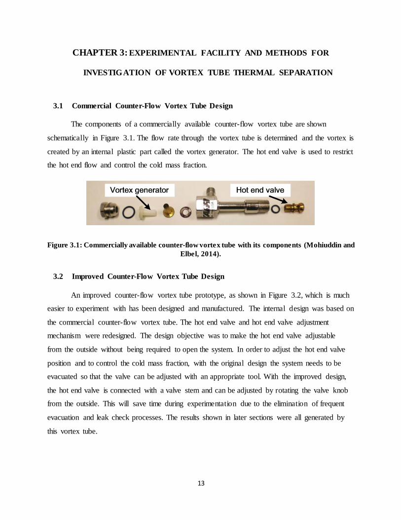
The components of a commercially available counter-flow vortex tube are shown
schematically in Figure 3.1. The flow rate through the vortex tube is determined and the vortex is
created by an internal plastic part called the vortex generator. The hot end valve is used to restrict
the hot end flow and control the cold mass fraction.
Figure 3.1: Commercially available counter-flow vortex tube with its components (Mohiuddin and
Elbel, 2014).
3.2 Improved Counter-Flow Vortex Tube Design
An improved counter-flow vortex tube prototype, as shown in Figure 3.2, which is much
easier to experiment with has been designed and manufactured. The internal design was based on
the commercial counter-flow vortex tube. The hot end valve and hot end valve adjustment
mechanism were redesigned. The design objective was to make the hot end valve adjustable
from the outside without being required to open the system. In order to adjust the hot end valve
position and to control the cold mass fraction, with the original design the system needs to be
evacuated so that the valve can be adjusted with an appropriate tool. With the improved design,
the hot end valve is connected with a valve stem and can be adjusted by rotating the valve knob
from the outside. This will save time during experimentation due to the elimination of frequent
evacuation and leak check processes. The results shown in later sections were all generated by
this vortex tube.
14
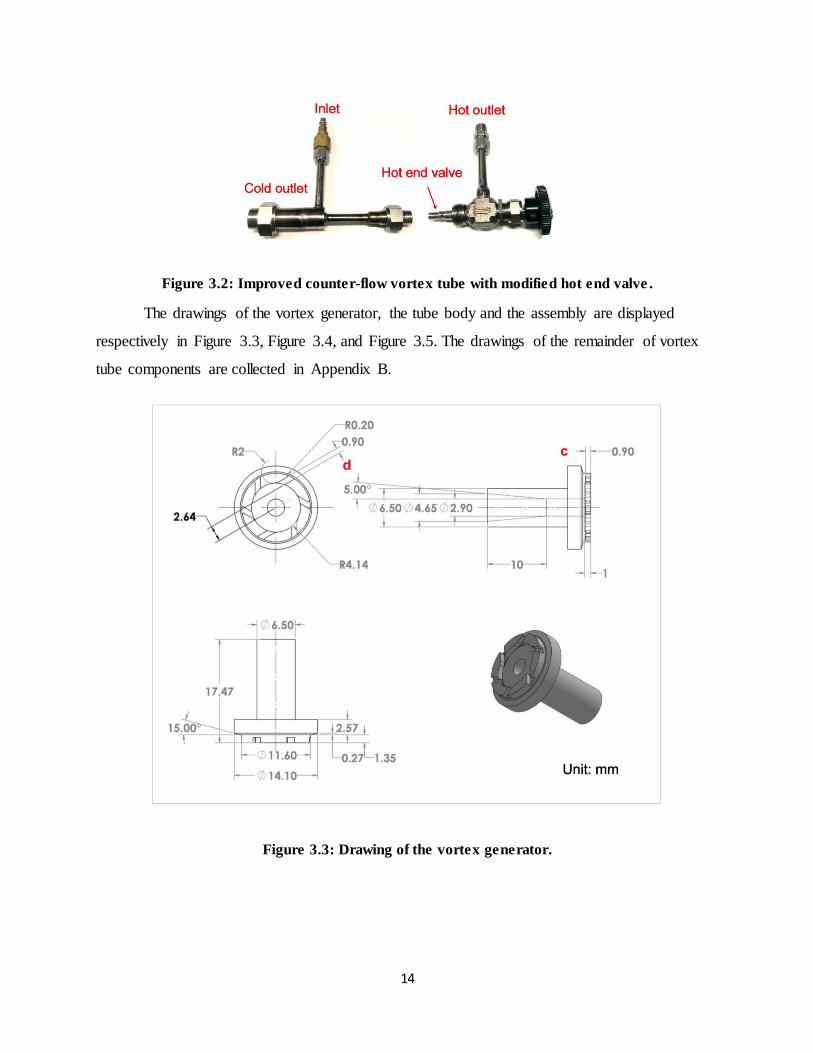
Figure 3.2: Improved counter-flow vortex tube with modified hot end valve .
The drawings of the vortex generator, the tube body and the assembly are displayed
respectively in Figure 3.3, Figure 3.4, and Figure 3.5. The drawings of the remainder of vortex
tube components are collected in Appendix B.
Figure 3.3: Drawing of the vortex generator.
15
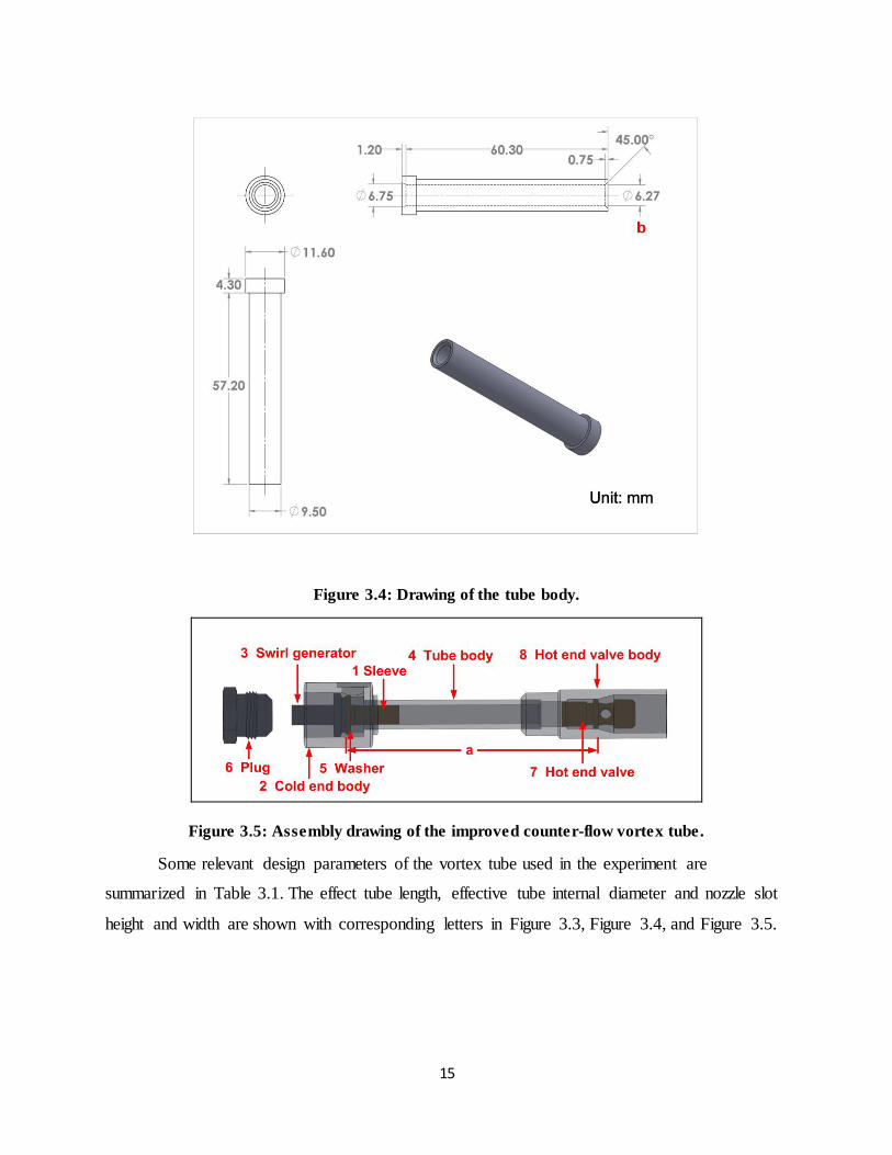
Figure 3.4: Drawing of the tube body.
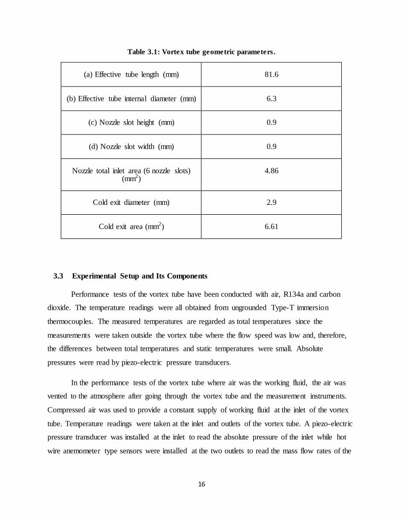
Figure 3.5: Assembly drawing of the improved counter-flow vortex tube.
Some relevant design parameters of the vortex tube used in the experiment are
summarized in Table 3.1. The effect tube length, effective tube internal diameter and nozzle slot
height and width are shown with corresponding letters in Figure 3.3, Figure 3.4, and Figure 3.5.
16
Table 3.1: Vortex tube geometric parameters.
(a) Effective tube length (mm) 81.6
(b) Effective tube internal diameter (mm) 6.3
(c) Nozzle slot height (mm) 0.9
(d) Nozzle slot width (mm) 0.9
Nozzle total inlet area (6 nozzle slots) (mm2)
4.86
Cold exit diameter (mm) 2.9
Cold exit area (mm2) 6.61
3.3 Experimental Setup and Its Components
Performance tests of the vortex tube have been conducted with air, R134a and carbon
dioxide. The temperature readings were all obtained from ungrounded Type-T immersion
thermocouples. The measured temperatures are regarded as total temperatures since the
measurements were taken outside the vortex tube where the flow speed was low and, therefore,
the differences between total temperatures and static temperatures were small. Absolute
pressures were read by piezo-electric pressure transducers.
In the performance tests of the vortex tube where air was the working fluid, the air was
vented to the atmosphere after going through the vortex tube and the measurement instruments.
Compressed air was used to provide a constant supply of working fluid at the inlet of the vortex
tube. Temperature readings were taken at the inlet and outlets of the vortex tube. A piezo-electric
pressure transducer was installed at the inlet to read the absolute pressure of the inlet while hot
wire anemometer type sensors were installed at the two outlets to read the mass flow rates of the
17
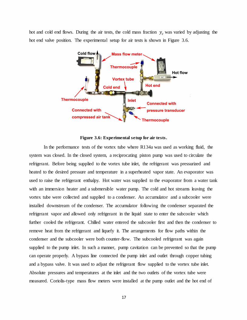
hot and cold end flows. During the air tests, the cold mass fraction 𝑦𝑐 was varied by adjusting the
hot end valve position. The experimental setup for air tests is shown in Figure 3.6.
Figure 3.6: Experimental setup for air tests .
In the performance tests of the vortex tube where R134a was used as working fluid, the
system was closed. In the closed system, a reciprocating piston pump was used to circulate the
refrigerant. Before being supplied to the vortex tube inlet, the refrigerant was pressurized and
heated to the desired pressure and temperature in a superheated vapor state. An evaporator was
used to raise the refrigerant enthalpy. Hot water was supplied to the evaporator from a water tank
with an immersion heater and a submersible water pump. The cold and hot streams leaving the
vortex tube were collected and supplied to a condenser. An accumulator and a subcooler were
installed downstream of the condenser. The accumulator following the condenser separated the
refrigerant vapor and allowed only refrigerant in the liquid state to enter the subcooler which
further cooled the refrigerant. Chilled water entered the subcooler first and then the condenser to
remove heat from the refrigerant and liquefy it. The arrangements for flow paths within the
condenser and the subcooler were both counter-flow. The subcooled refrigerant was again
supplied to the pump inlet. In such a manner, pump cavitation can be prevented so that the pump
can operate properly. A bypass line connected the pump inlet and outlet through copper tubing
and a bypass valve. It was used to adjust the refrigerant flow supplied to the vortex tube inlet.
Absolute pressures and temperatures at the inlet and the two outlets of the vortex tube were
measured. Coriolis-type mass flow meters were installed at the pump outlet and the hot end of
18
the vortex tube where the refrigerant flow was single-phase. Sight glasses were installed at
various locations of the system to monitor the refrigerant flow. During the experimental tests, the
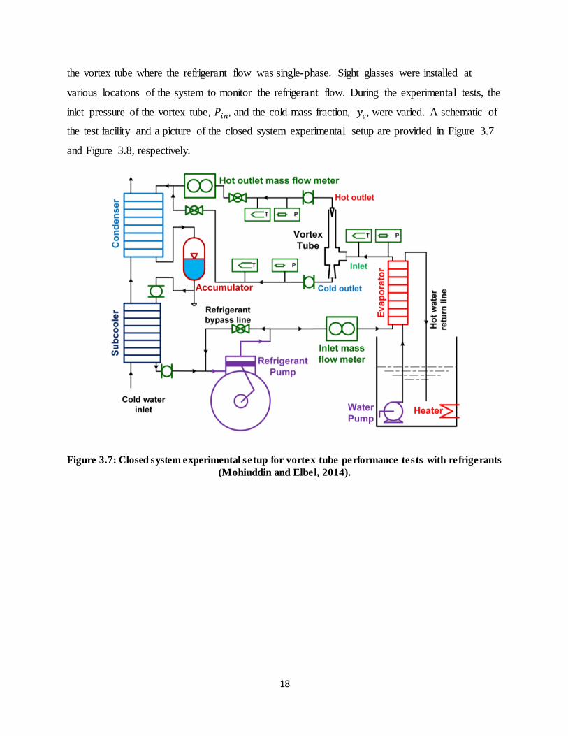
inlet pressure of the vortex tube, 𝑃𝑖𝑛, and the cold mass fraction, 𝑦𝑐, were varied. A schematic of
the test facility and a picture of the closed system experimental setup are provided in Figure 3.7
and Figure 3.8, respectively.
Figure 3.7: Closed system experimental setup for vortex tube performance tests with refrigerants
(Mohiuddin and Elbel, 2014).
19
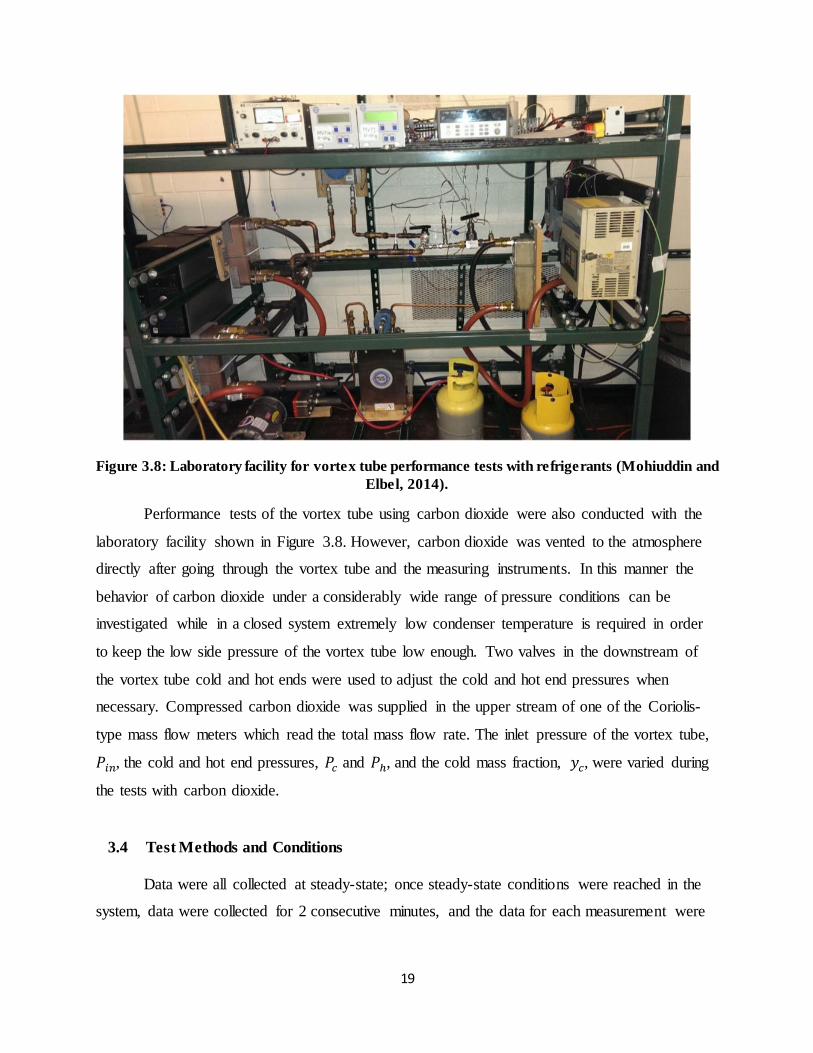
Figure 3.8: Laboratory facility for vortex tube performance tests with refrigerants (Mohiuddin and
Elbel, 2014).
Performance tests of the vortex tube using carbon dioxide were also conducted with the
laboratory facility shown in Figure 3.8. However, carbon dioxide was vented to the atmosphere
directly after going through the vortex tube and the measuring instruments. In this manner the
behavior of carbon dioxide under a considerably wide range of pressure conditions can be
investigated while in a closed system extremely low condenser temperature is required in order
to keep the low side pressure of the vortex tube low enough. Two valves in the downstream of
the vortex tube cold and hot ends were used to adjust the cold and hot end pressures when
necessary. Compressed carbon dioxide was supplied in the upper stream of one of the Coriolis-
type mass flow meters which read the total mass flow rate. The inlet pressure of the vortex tube,
𝑃𝑖𝑛, the cold and hot end pressures, 𝑃𝑐 and 𝑃ℎ, and the cold mass fraction, 𝑦𝑐, were varied during
the tests with carbon dioxide.
3.4 Test Methods and Conditions
Data were all collected at steady-state; once steady-state conditions were reached in the
system, data were collected for 2 consecutive minutes, and the data for each measurement were
20
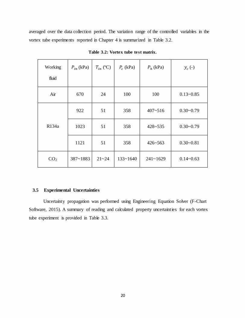
averaged over the data collection period. The variation range of the controlled variables in the
vortex tube experiments reported in Chapter 4 is summarized in Table 3.2.
Table 3.2: Vortex tube test matrix.
Working
fluid
𝑃𝑖𝑛 (kPa) 𝑇𝑖𝑛 (ºC) 𝑃𝑐 (kPa) 𝑃ℎ (kPa) 𝑦𝑐 (-)
Air 670 24 100 100 0.13~0.85
R134a
922 51 358 407~516 0.30~0.79
1023 51 358 428~535 0.30~0.79
1121 51 358 426~563 0.30~0.81
CO2 387~1883 21~24 133~1640 241~1629 0.14~0.63
3.5 Experimental Uncertainties
Uncertainty propagation was performed using Engineering Equation Solver (F-Chart
Software, 2015). A summary of reading and calculated property uncertainties for each vortex
tube experiment is provided in Table 3.3.
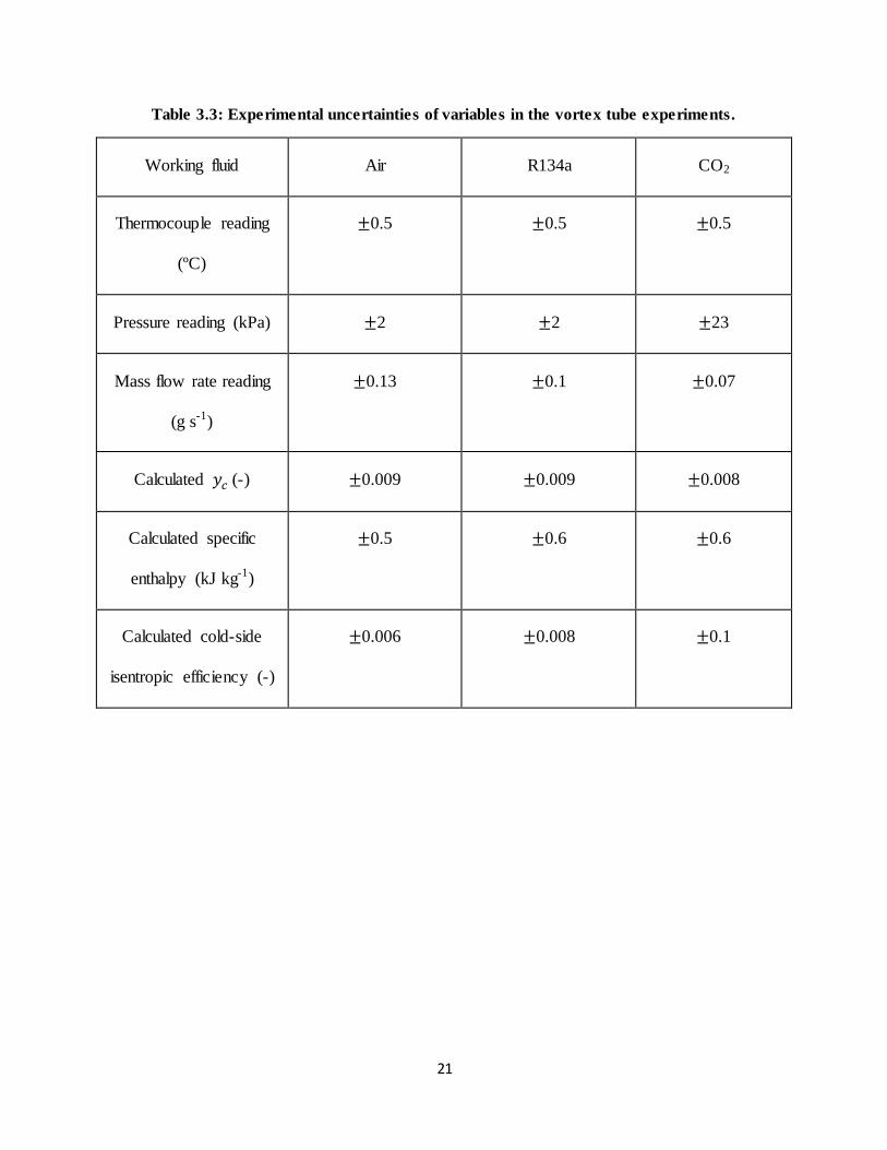
21
Table 3.3: Experimental uncertainties of variables in the vortex tube experiments.
Working fluid Air R134a CO2
Thermocouple reading
(ºC)
±0.5 ±0.5 ±0.5
Pressure reading (kPa) ±2 ±2 ±23
Mass flow rate reading
(g s-1)
±0.13 ±0.1 ±0.07
Calculated 𝑦𝑐 (-) ±0.009 ±0.009 ±0.008
Calculated specific
enthalpy (kJ kg-1)
±0.5 ±0.6 ±0.6
Calculated cold-side
isentropic efficiency (-)
±0.006 ±0.008 ±0.1
22
CHAPTER 4: EXPERIMENTAL INVESTIGATION OF VORTEX TUBE
THERMAL SEPARATION
Air, R134a, and carbon dioxide were used as working fluids in the vortex tube
performance tests. Inside the vortex tube the working fluid was always kept in the superheated
vapor state, since thermal separation can be impaired or even completely diminished once there
is two-phase flow inside the tube. The contact of superheated vapor with liquid will result in
boiling of liquid and cooling of superheated vapor until saturation is reached and temperature
difference disappears. In principle, vortex tubes can generate temperature separation with single-
phase liquid. However, subcooled liquid has much larger specific heat than superheated vapor
and has much less difference in specific enthalpy between the isentropic and isenthalpic
expansions. Therefore, it does not produce as much temperature difference between the two ends
of the vortex tube as superheated vapor does for the same pressure drop, and thus is not studied
in this project.
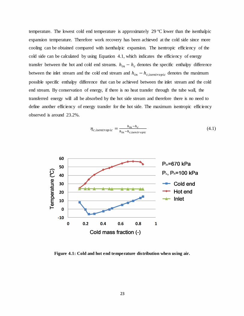
4.1 Experimental Results with Air
Figure 4.1 shows the temperature separation achieved by the vortex tube for different
cold mass fractions when air is the working fluid. The inlet temperature and pressure are 24.0 ºC
and 670 kPa, respectively, while the outlets are at atmospheric pressure. Total mass flow rate
through the vortex tube inlet ranges from 5.1 g s-1 to 7.7 g s-1. The highest hot end temperature is
reached at 56.6 ºC when 𝑦𝑐 = 0.74 and the lowest cold end temperature is achieved at -5.9 ºC
when 𝑦𝑐 = 0.24. As mentioned previously, the highest hot end and the lowest cold end
temperatures are achieved with different settings of the hot end valve. The hot end temperature is
higher than the inlet temperature while the cold end temperature is lower than the inlet
temperature. These results are in good agreement with experimental results with air in the
literature (Stephan et al., 1983).
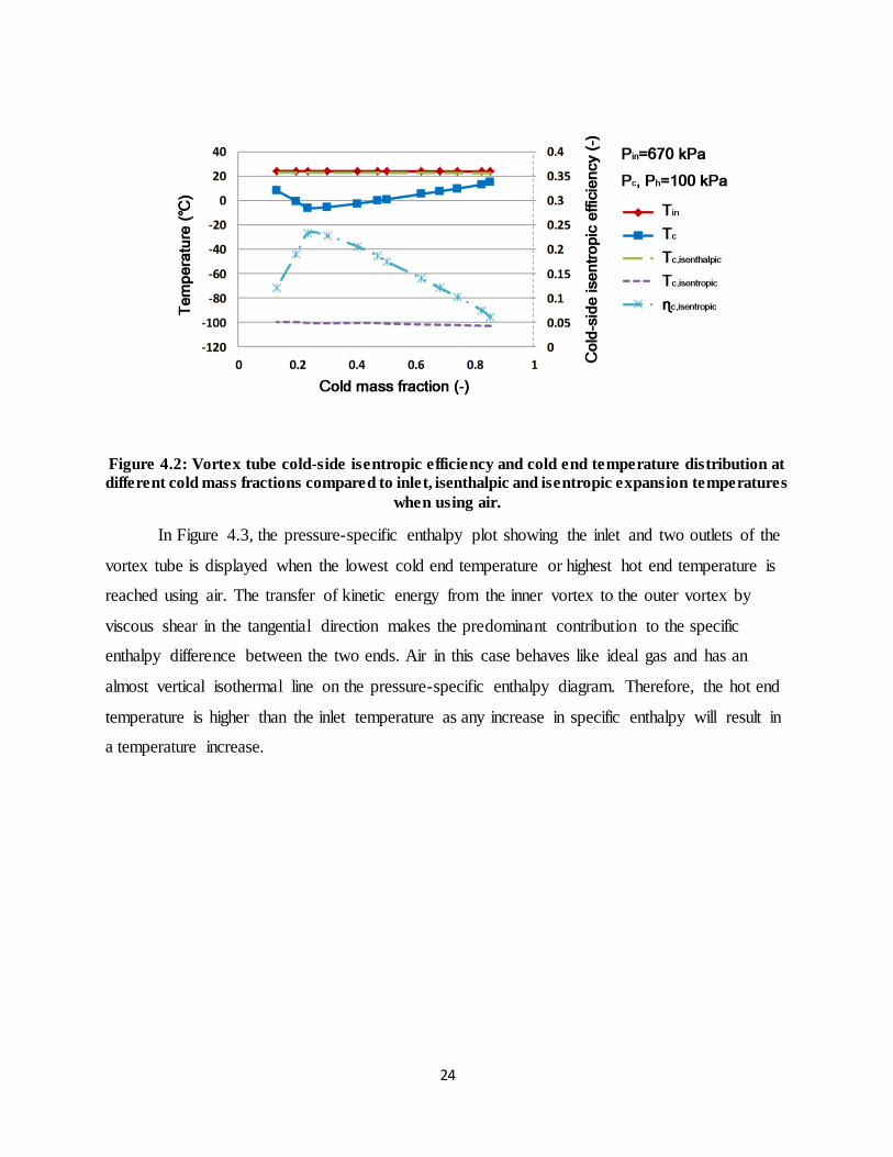
Figure 4.2 compares the vortex tube cold end temperature distribution at different cold
mass fractions with the inlet temperature, as well as the calculated temperatures of air if going
through an isenthalpic or isentropic process between the inlet and outlet pressures. It can be
observed that the cold end temperature is always lower than the isenthalpic expansion
23
temperature. The lowest cold end temperature is approximately 29 ºC lower than the isenthalpic
expansion temperature. Therefore work recovery has been achieved at the cold side since more
cooling can be obtained compared with isenthalpic expansion. The isentropic efficiency of the
cold side can be calculated by using Equation 4.1, which indicates the efficiency of energy
transfer between the hot and cold end streams. ℎ𝑖𝑛 − ℎ𝑐 denotes the specific enthalpy difference
between the inlet stream and the cold end stream and ℎ𝑖𝑛 − ℎ𝑐,𝑖𝑠𝑒𝑛𝑡𝑟𝑜𝑝𝑖𝑐 denotes the maximum
possible specific enthalpy difference that can be achieved between the inlet stream and the cold
end stream. By conservation of energy, if there is no heat transfer through the tube wall, the
transferred energy will all be absorbed by the hot side stream and therefore there is no need to
define another efficiency of energy transfer for the hot side. The maximum isentropic efficiency
observed is around 23.2%.
𝜂𝑐,𝑖𝑠𝑒𝑛𝑡𝑟𝑜𝑝𝑖𝑐 =ℎ𝑖𝑛 −ℎ𝑐
ℎ𝑖𝑛 −ℎ𝑐,𝑖𝑠𝑒𝑛𝑡𝑟𝑜𝑝𝑖𝑐 (4.1)
Figure 4.1: Cold and hot end temperature distribution when using air.
24
Figure 4.2: Vortex tube cold-side isentropic efficiency and cold end temperature distribution at
different cold mass fractions compared to inlet, isenthalpic and isentropic expansion temperatures
when using air.
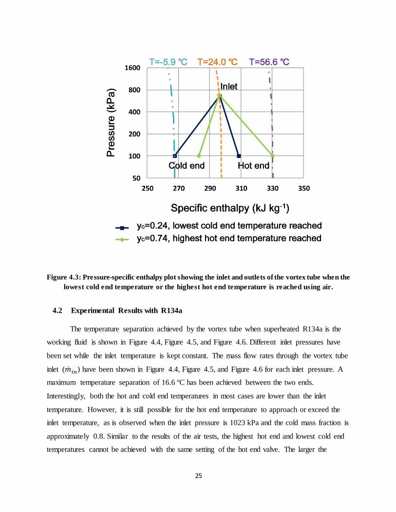
In Figure 4.3, the pressure-specific enthalpy plot showing the inlet and two outlets of the
vortex tube is displayed when the lowest cold end temperature or highest hot end temperature is
reached using air. The transfer of kinetic energy from the inner vortex to the outer vortex by
viscous shear in the tangential direction makes the predominant contribution to the specific
enthalpy difference between the two ends. Air in this case behaves like ideal gas and has an
almost vertical isothermal line on the pressure-specific enthalpy diagram. Therefore, the hot end
temperature is higher than the inlet temperature as any increase in specific enthalpy will result in
a temperature increase.
25
Figure 4.3: Pressure-specific enthalpy plot showing the inlet and outlets of the vortex tube when the
lowest cold end temperature or the highest hot end temperature is reached using air.
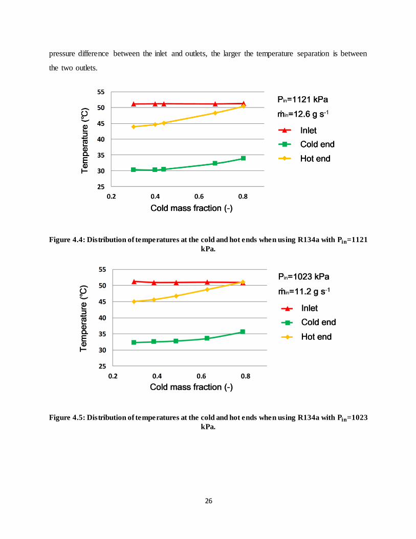
4.2 Experimental Results with R134a
The temperature separation achieved by the vortex tube when superheated R134a is the
working fluid is shown in Figure 4.4, Figure 4.5, and Figure 4.6. Different inlet pressures have
been set while the inlet temperature is kept constant. The mass flow rates through the vortex tube
inlet (�̇�𝑖𝑛) have been shown in Figure 4.4, Figure 4.5, and Figure 4.6 for each inlet pressure. A
maximum temperature separation of 16.6 ºC has been achieved between the two ends.
Interestingly, both the hot and cold end temperatures in most cases are lower than the inlet
temperature. However, it is still possible for the hot end temperature to approach or exceed the
inlet temperature, as is observed when the inlet pressure is 1023 kPa and the cold mass fraction is
approximately 0.8. Similar to the results of the air tests, the highest hot end and lowest cold end
temperatures cannot be achieved with the same setting of the hot end valve. The larger the
26
pressure difference between the inlet and outlets, the larger the temperature separation is between
the two outlets.
Figure 4.4: Distribution of temperatures at the cold and hot ends when using R134a with 𝐏𝐢𝐧=1121
kPa.
Figure 4.5: Distribution of temperatures at the cold and hot ends when using R134a with 𝐏𝐢𝐧=1023
kPa.
27
Figure 4.6: Distribution of temperatures at the cold and hot ends when using R134a with 𝐏𝐢𝐧=922
kPa.
Figure 4.7 shows the comparison of the vortex tube cold end temperature with the inlet
temperature, and the calculated isenthalpic and isentropic expansion temperatures at different
cold mass fractions when the working fluid is superheated R134a. The cold end temperature is
always lower than the isenthalpic expansion temperature which indicates that work recovery has
been achieved. The lowest cold end temperature is 6 ºC lower than the isenthalpic expansion
temperature. The maximum isentropic efficiency observed is around 22%, comparable to the
efficiencies achieved with air.
28
Figure 4.7: Vortex tube cold-side isentropic efficiency and cold end temperature distribution at
different cold mass fractions compared to inlet, isenthalpic and isentropic expansion temperatures
when using R134a.
Figure 4.8, Figure 4.9, and Figure 4.10 display the pressure-specific enthalpy plots
showing the inlet and two outlets of the vortex tube for different cold mass fractions when R134a
is the working fluid. Because of the mass flow meter in the downstream of the hot end, there is a
small pressure difference between the hot and cold outlets. Similarly to the results of air tests, a
significant specific enthalpy difference between the two ends can be observed because of the
kinetic energy transfer between the two streams. At the test conditions considered, R134a is
close to the saturation dome and its superheated vapor shows non-ideal gas behavior. The
isothermal lines on the pressure-specific enthalpy diagram have negative slopes so that after the
pressure drop a large specific enthalpy increase would be required in order to have the hot end
temperature higher than the inlet temperature. For ideal gases like air, specific enthalpy is only
dependent on temperature and any increase in specific enthalpy will result in increase in
temperature. This is the reason why when air is used as vortex tube working fluid, the hot end
temperature is always higher than the inlet temperature, while when R134a is used the hot end
temperature in most cases is lower than the inlet temperature. However, as shown in Figure 4.9,
depending on the test conditions, it is still possible to observe the hot end temperature approach
or exceed the inlet temperature.
29
Figure 4.8: Pressure-specific enthalpy plot showing the vortex tube inlet and outlets when using
R134a with 𝐏𝐢𝐧=1121 kPa.
Figure 4.9: Pressure-specific enthalpy plot showing the vortex tube inlet and outlets when using
R134a with 𝐏𝐢𝐧=1023 kPa.
30
Figure 4.10: Pressure-specific enthalpy plot showing the vortex tube inlet and outlets when using
R134a with 𝐏𝐢𝐧=922 kPa.
4.3 Experimental Results with Carbon Dioxide
Pressures and specific enthalpies at the vortex tube inlet and outlets for carbon dioxide as
the working fluid were investigated next. Figure 4.11 and Figure 4.12 show results for low and
high cold mass fractions, respectively. During all the experiments, it was always observed that
the specific enthalpy at the hot end increases and the specific enthalpy at the cold end decreases
compared with inlet specific enthalpy. At the lower pressure region, the hot end temperature can
become higher than that of the inlet while at the higher pressure region, both the cold and hot end
temperatures are lower than the inlet. Whether the hot end temperature can be higher than the
inlet depends on whether the vapor behaves like ideal gas. When the inlet pressure and
temperature are, respectively, 865 kPa and 22.6 ºC, if the pressure is dropped by half, an increase
of 4.31 kPa kg kJ-1 in specific enthalpy is required to keep the vapor temperature the same.
Meanwhile, if the inlet pressure and temperature are 387 kPa and 22.6 ºC, an increase of only
1.864 kPa kg kJ-1 in specific enthalpy is required to keep the vapor temperature constant after the
pressure is dropped by half.
31
Figure 4.11: Pressure-specific enthalpy plot showing the vortex tube inlet and outlets when using
carbon dioxide at small cold mass fractions .
Figure 4.12: Pressure-specific enthalpy plot showing the vortex tube inlet and outlets when using
carbon dioxide at large cold mass fractions.
32
The specific enthalpy of an ideal gas is independent of the pressure. For ideal gas, no
increase in the specific enthalpy is needed after pressure drop to keep the temperature constant.
Therefore, at lower pressure, vapor shows more ideal gas behavior and a smaller specific
enthalpy increase is required after pressure drop with the same pressure ratio for the hot end
temperature to be higher than the inlet. At higher temperature, vapor will also behave more like
ideal gas and it will be easier for the hot end temperature of the vortex tube to exceed the inlet
temperature.
33
CHAPTER 5: NUMERICAL ANALYSIS OF POSSIBLE VORTEX TUBE
CYCLES FOR COOLING AND HEATING
The preceding experiments have shown that vortex tubes can produce significant thermal
separation when all fluid streams remain single-phase vapor inside the tube. Once there is two-
phase flow inside the tube, thermal separation can be impaired or even entirely eliminated. It can
be concluded that vortex tubes cannot be used as a simple replacement for the expansion device
of a conventional vapor compression cycle for two reasons: a) two-phase flow is present at the
end of the expansion process when reducing the refrigerant pressure between condenser and
evaporator; b) subcooled liquid does not produce as much temperature difference between the
two ends of the vortex tube as superheated vapor does for the same pressure drop. These
characteristics need to be taken into account when devising heating and cooling cycles with
vortex tubes where thermal separation is required.
Moreover, the specific enthalpy of an ideal gas is only dependent on the temperature.
Therefore, any changes in specific enthalpy could result in changes in temperature. This explains
why hot end temperatures higher than inlet temperature can be more easily achieved with air or
low-pressure carbon dioxide as the working fluid, but have not been frequently observed in the
experiments carried out with R134a vapor whose fluid properties resemble less of ideal gas
behavior under the conditions considered. If the heating feature of the vortex tube needs to be
utilized, the working fluid inside the vortex tube should behave like an ideal gas.
There is a transfer of kinetic energy between the two streams inside the vortex tube due to
the viscous shear in the tangential direction, much like the energy transfer occurring inside
ejectors and expanders. However, the kinetic energy transferred to the hot stream in the vortex
tube is turned into heat, while in an ejector and an expander the kinetic energy transferred is used
to raise the compressor inlet pressure or turned into shaft power that is used to reduce the work
input to the compressor. The energy transfer and the resulting temperature differences in a vortex
tube can be utilized in two different ways. In order to successfully apply vortex tubes to cooling
cycles, the cold side can be utilized to provide more cooling than isenthalpic expansion and the
additional heat needs to be rejected without increasing compressor work. In heating applications,
the temperature at the vortex tube hot side can be raised to higher levels than the inlet
34
temperature. As explained before, working fluids which show ideal gas behavior should be
chosen in such applications.
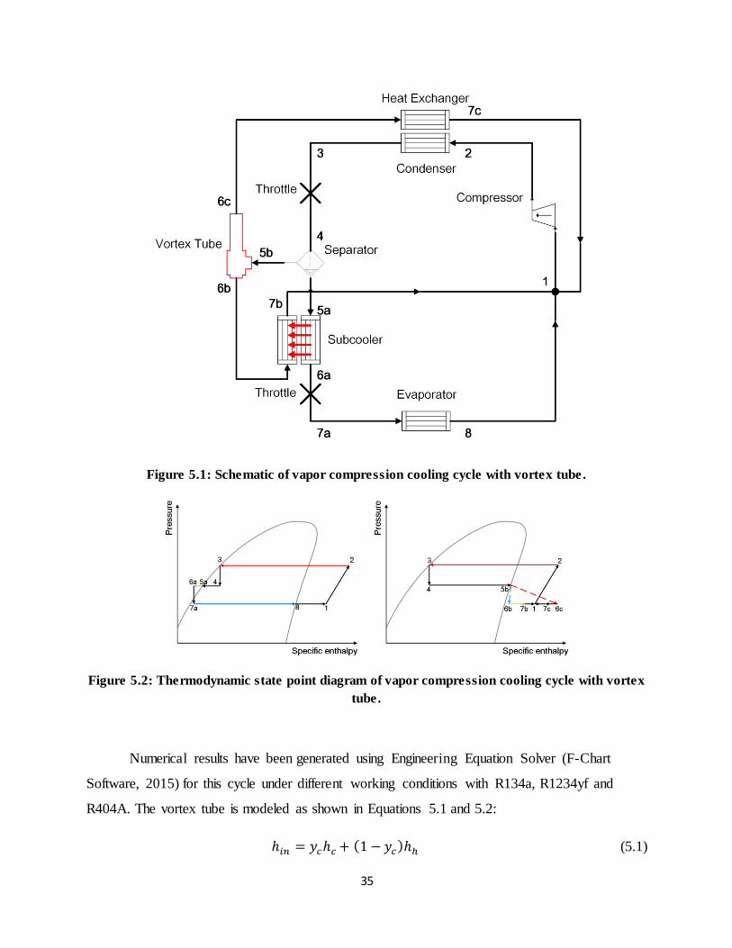
5.1 Vortex Tube Cooling Cycle
An example of a possible cooling cycle utilizing vortex tube expansion is shown in
Figure 5.1 and Figure 5.2. Flow at state (3) at the condenser outlet undergoes a first throttling
process. Vapor and liquid are then separated and the saturated liquid at state (5a) is fed into the
internal heat exchanger and gets subcooled by flow from (6b). Flow at state (5b) is the flash gas
generated during the first expansion process from state (3) to state (4). It is fed into the vortex
tube to produce thermal separation. If the hot stream at state (6c) coming out of the vortex tube
has higher temperature than the ambient, it can be cooled to the ambient temperature by heat
exchange with the ambient. The cold stream at state (6b) gets superheated in the internal heat
exchanger. More cooling capacity in the evaporator is achieved without incurring more
compressor work by using the cold stream to subcool the saturated liquid at the condenser outlet
compared with baseline cycle without vortex tube. In such a manner COP of the cycle is
improved. An additional internal heat exchanger can be added to superheat the flow at state (5b)
at the vortex tube inlet with the flow at state (3) so that two-phase flow can be avoided inside the
vortex tube for all working fluids (Keller et al., 1997; Christensen et al., 2001).
35
Figure 5.1: Schematic of vapor compression cooling cycle with vortex tube.
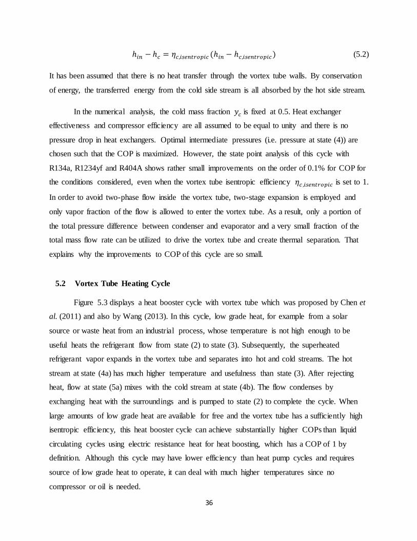
Figure 5.2: Thermodynamic state point diagram of vapor compression cooling cycle with vortex
tube.
Numerical results have been generated using Engineering Equation Solver (F-Chart
Software, 2015) for this cycle under different working conditions with R134a, R1234yf and
R404A. The vortex tube is modeled as shown in Equations 5.1 and 5.2:
ℎ𝑖𝑛 = 𝑦𝑐ℎ𝑐 + (1 − 𝑦𝑐)ℎℎ (5.1)
36
ℎ𝑖𝑛 − ℎ𝑐 = 𝜂𝑐,𝑖𝑠𝑒𝑛𝑡𝑟𝑜𝑝𝑖𝑐 (ℎ𝑖𝑛 − ℎ𝑐,𝑖𝑠𝑒𝑛𝑡𝑟𝑜𝑝𝑖𝑐 ) (5.2)
It has been assumed that there is no heat transfer through the vortex tube walls. By conservation
of energy, the transferred energy from the cold side stream is all absorbed by the hot side stream.
In the numerical analysis, the cold mass fraction 𝑦𝑐 is fixed at 0.5. Heat exchanger
effectiveness and compressor efficiency are all assumed to be equal to unity and there is no
pressure drop in heat exchangers. Optimal intermediate pressures (i.e. pressure at state (4)) are
chosen such that the COP is maximized. However, the state point analysis of this cycle with
R134a, R1234yf and R404A shows rather small improvements on the order of 0.1% for COP for
the conditions considered, even when the vortex tube isentropic efficiency 𝜂𝑐 ,𝑖𝑠𝑒𝑛𝑡𝑟𝑜𝑝𝑖𝑐 is set to 1.
In order to avoid two-phase flow inside the vortex tube, two-stage expansion is employed and
only vapor fraction of the flow is allowed to enter the vortex tube. As a result, only a portion of
the total pressure difference between condenser and evaporator and a very small fraction of the
total mass flow rate can be utilized to drive the vortex tube and create thermal separation. That
explains why the improvements to COP of this cycle are so small.
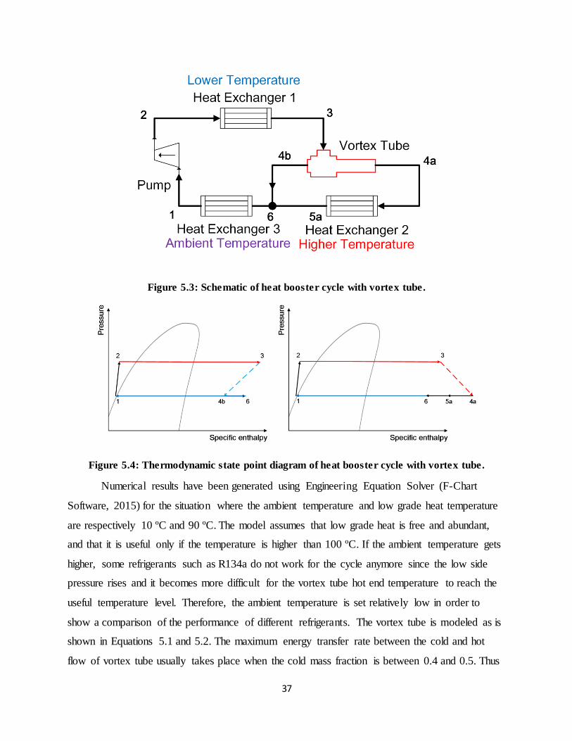
5.2 Vortex Tube Heating Cycle
Figure 5.3 displays a heat booster cycle with vortex tube which was proposed by Chen et
al. (2011) and also by Wang (2013). In this cycle, low grade heat, for example from a solar
source or waste heat from an industrial process, whose temperature is not high enough to be
useful heats the refrigerant flow from state (2) to state (3). Subsequently, the superheated
refrigerant vapor expands in the vortex tube and separates into hot and cold streams. The hot
stream at state (4a) has much higher temperature and usefulness than state (3). After rejecting
heat, flow at state (5a) mixes with the cold stream at state (4b). The flow condenses by
exchanging heat with the surroundings and is pumped to state (2) to complete the cycle. When
large amounts of low grade heat are available for free and the vortex tube has a sufficiently high
isentropic efficiency, this heat booster cycle can achieve substantially higher COPs than liquid
circulating cycles using electric resistance heat for heat boosting, which has a COP of 1 by
definition. Although this cycle may have lower efficiency than heat pump cycles and requires
source of low grade heat to operate, it can deal with much higher temperatures since no
compressor or oil is needed.
37
Figure 5.3: Schematic of heat booster cycle with vortex tube.
Figure 5.4: Thermodynamic state point diagram of heat booster cycle with vortex tube.
Numerical results have been generated using Engineering Equation Solver (F-Chart
Software, 2015) for the situation where the ambient temperature and low grade heat temperature
are respectively 10 ºC and 90 ºC. The model assumes that low grade heat is free and abundant,
and that it is useful only if the temperature is higher than 100 ºC. If the ambient temperature gets
higher, some refrigerants such as R134a do not work for the cycle anymore since the low side
pressure rises and it becomes more difficult for the vortex tube hot end temperature to reach the
useful temperature level. Therefore, the ambient temperature is set relatively low in order to
show a comparison of the performance of different refrigerants. The vortex tube is modeled as is
shown in Equations 5.1 and 5.2. The maximum energy transfer rate between the cold and hot
flow of vortex tube usually takes place when the cold mass fraction is between 0.4 and 0.5. Thus
38
the cold mass fraction of the vortex tube is fixed at 0.5, which is close to the maximum energy
transfer rate point. Ideal heat exchangers and pump are assumed in the calculation. COP of the
cycle is defined as the ratio of the heating capacity to the pump power as is shown in Equation
5.3:
𝐶𝑂𝑃ℎ𝑒𝑎𝑡 𝑏𝑜𝑜𝑠𝑡𝑒𝑟 =𝑄ℎ𝑒𝑎𝑡𝑖𝑛𝑔
𝑊𝑝𝑢𝑚𝑝= (1 − 𝑦𝑐) ∗
ℎ4𝑎−ℎ5𝑎
ℎ2−ℎ1 (5.3)
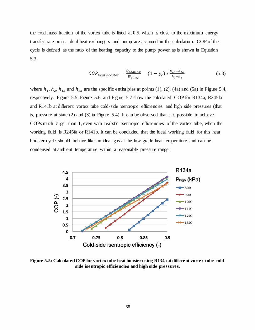
where ℎ1, ℎ2, ℎ4𝑎 and ℎ5𝑎 are the specific enthalpies at points (1), (2), (4a) and (5a) in Figure 5.4,
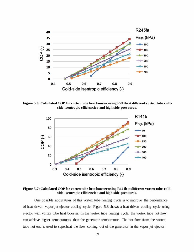
respectively. Figure 5.5, Figure 5.6, and Figure 5.7 show the calculated COP for R134a, R245fa
and R141b at different vortex tube cold-side isentropic efficiencies and high side pressures (that
is, pressure at state (2) and (3) in Figure 5.4). It can be observed that it is possible to achieve
COPs much larger than 1, even with realistic isentropic efficiencies of the vortex tube, when the
working fluid is R245fa or R141b. It can be concluded that the ideal working fluid for this heat
booster cycle should behave like an ideal gas at the low grade heat temperature and can be
condensed at ambient temperature within a reasonable pressure range.
Figure 5.5: Calculated COP for vortex tube heat booster using R134a at different vortex tube cold-
side isentropic efficiencies and high side pressures.
39
Figure 5.6: Calculated COP for vortex tube heat booster using R245fa at different vortex tube cold-
side isentropic efficiencies and high side pressures.
Figure 5.7: Calculated COP for vortex tube heat booster using R141b at different vortex tube cold-
side isentropic efficiencies and high side pressures.
One possible application of this vortex tube heating cycle is to improve the performance
of heat driven vapor jet ejector cooling cycle. Figure 5.8 shows a heat driven cooling cycle using
ejector with vortex tube heat booster. In the vortex tube heating cycle, the vortex tube hot flow
can achieve higher temperatures than the generator temperature. The hot flow from the vortex
tube hot end is used to superheat the flow coming out of the generator in the vapor jet ejector
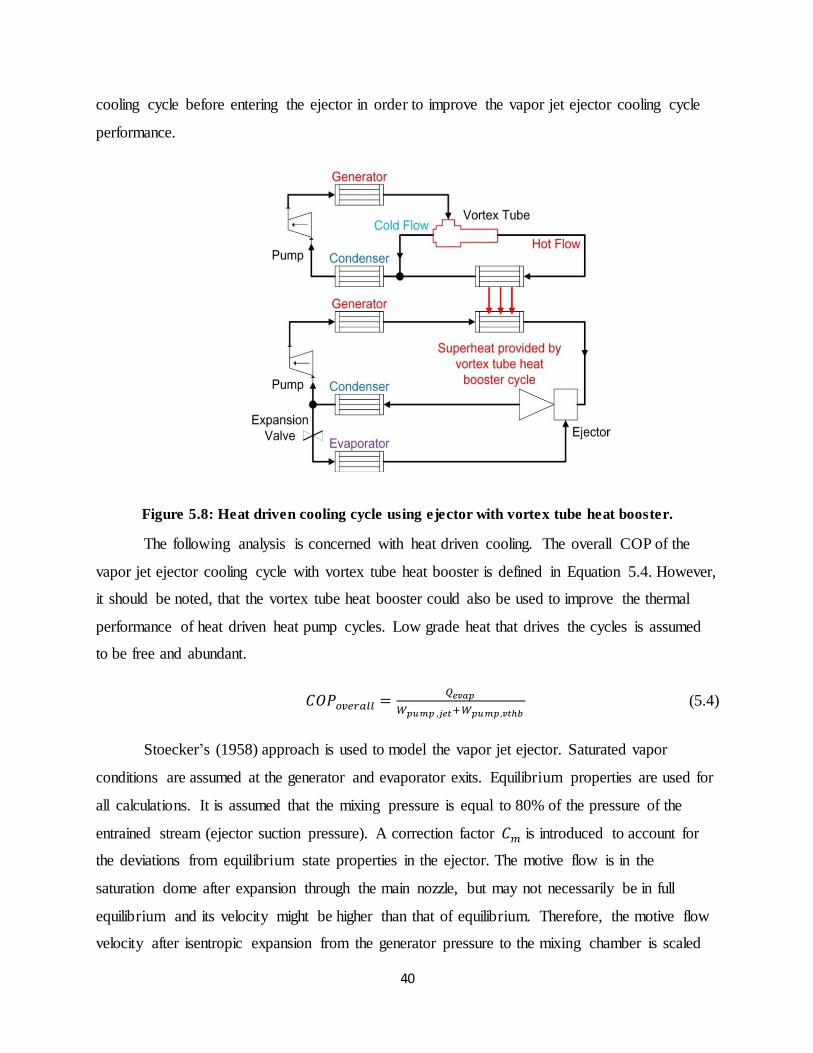
40
cooling cycle before entering the ejector in order to improve the vapor jet ejector cooling cycle
performance.
Figure 5.8: Heat driven cooling cycle using ejector with vortex tube heat booster.
The following analysis is concerned with heat driven cooling. The overall COP of the
vapor jet ejector cooling cycle with vortex tube heat booster is defined in Equation 5.4. However,
it should be noted, that the vortex tube heat booster could also be used to improve the thermal
performance of heat driven heat pump cycles. Low grade heat that drives the cycles is assumed
to be free and abundant.
𝐶𝑂𝑃𝑜𝑣𝑒𝑟𝑎𝑙𝑙 =𝑄𝑒𝑣𝑎𝑝
𝑊𝑝𝑢𝑚𝑝 ,𝑗𝑒𝑡+𝑊𝑝𝑢𝑚𝑝,𝑣𝑡ℎ𝑏 (5.4)
Stoecker’s (1958) approach is used to model the vapor jet ejector. Saturated vapor
conditions are assumed at the generator and evaporator exits. Equilibrium properties are used for
all calculations. It is assumed that the mixing pressure is equal to 80% of the pressure of the
entrained stream (ejector suction pressure). A correction factor 𝐶𝑚 is introduced to account for
the deviations from equilibrium state properties in the ejector. The motive flow is in the
saturation dome after expansion through the main nozzle, but may not necessarily be in full
equilibrium and its velocity might be higher than that of equilibrium. Therefore, the motive flow
velocity after isentropic expansion from the generator pressure to the mixing chamber is scaled
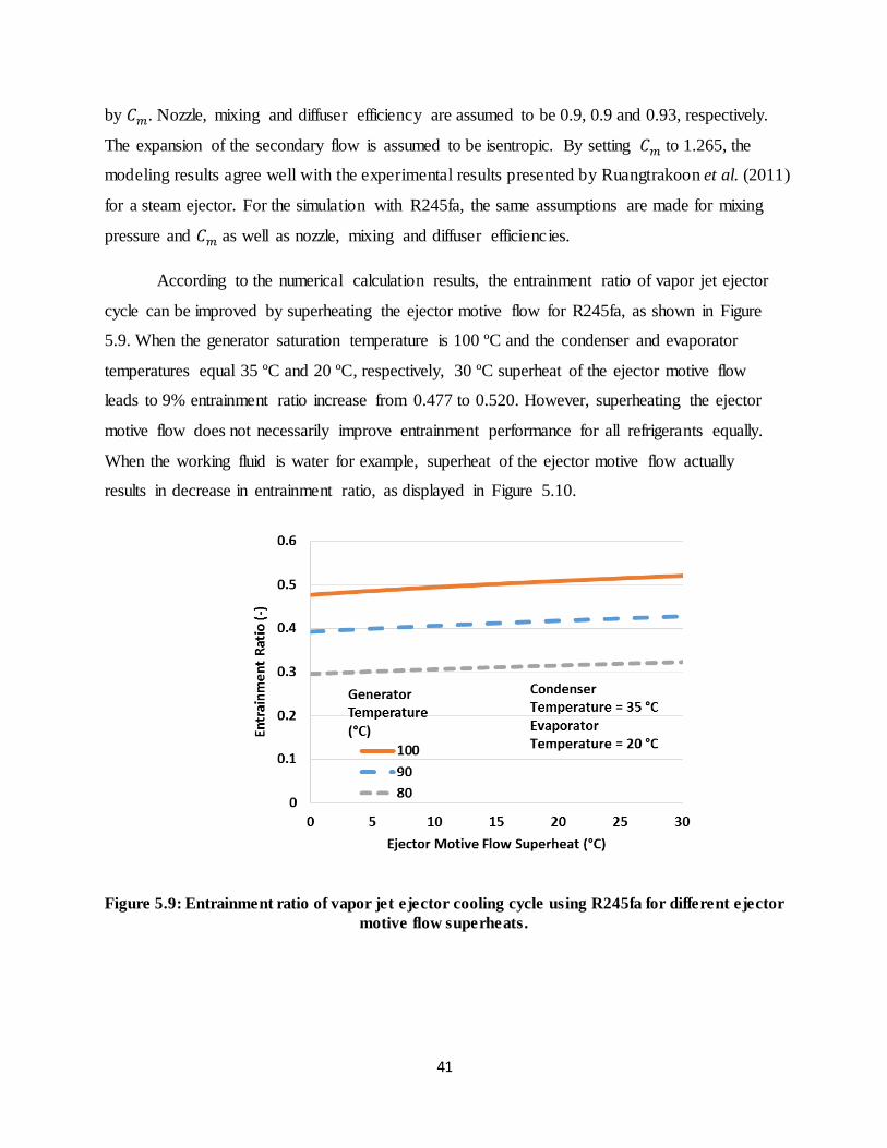
41
by 𝐶𝑚. Nozzle, mixing and diffuser efficiency are assumed to be 0.9, 0.9 and 0.93, respectively.
The expansion of the secondary flow is assumed to be isentropic. By setting 𝐶𝑚 to 1.265, the
modeling results agree well with the experimental results presented by Ruangtrakoon et al. (2011)
for a steam ejector. For the simulation with R245fa, the same assumptions are made for mixing
pressure and 𝐶𝑚 as well as nozzle, mixing and diffuser efficiencies.
According to the numerical calculation results, the entrainment ratio of vapor jet ejector
cycle can be improved by superheating the ejector motive flow for R245fa, as shown in Figure
5.9. When the generator saturation temperature is 100 ºC and the condenser and evaporator
temperatures equal 35 ºC and 20 ºC, respectively, 30 ºC superheat of the ejector motive flow
leads to 9% entrainment ratio increase from 0.477 to 0.520. However, superheating the ejector
motive flow does not necessarily improve entrainment performance for all refrigerants equally.
When the working fluid is water for example, superheat of the ejector motive flow actually
results in decrease in entrainment ratio, as displayed in Figure 5.10.
Figure 5.9: Entrainment ratio of vapor jet ejector cooling cycle using R245fa for different ejector
motive flow superheats.
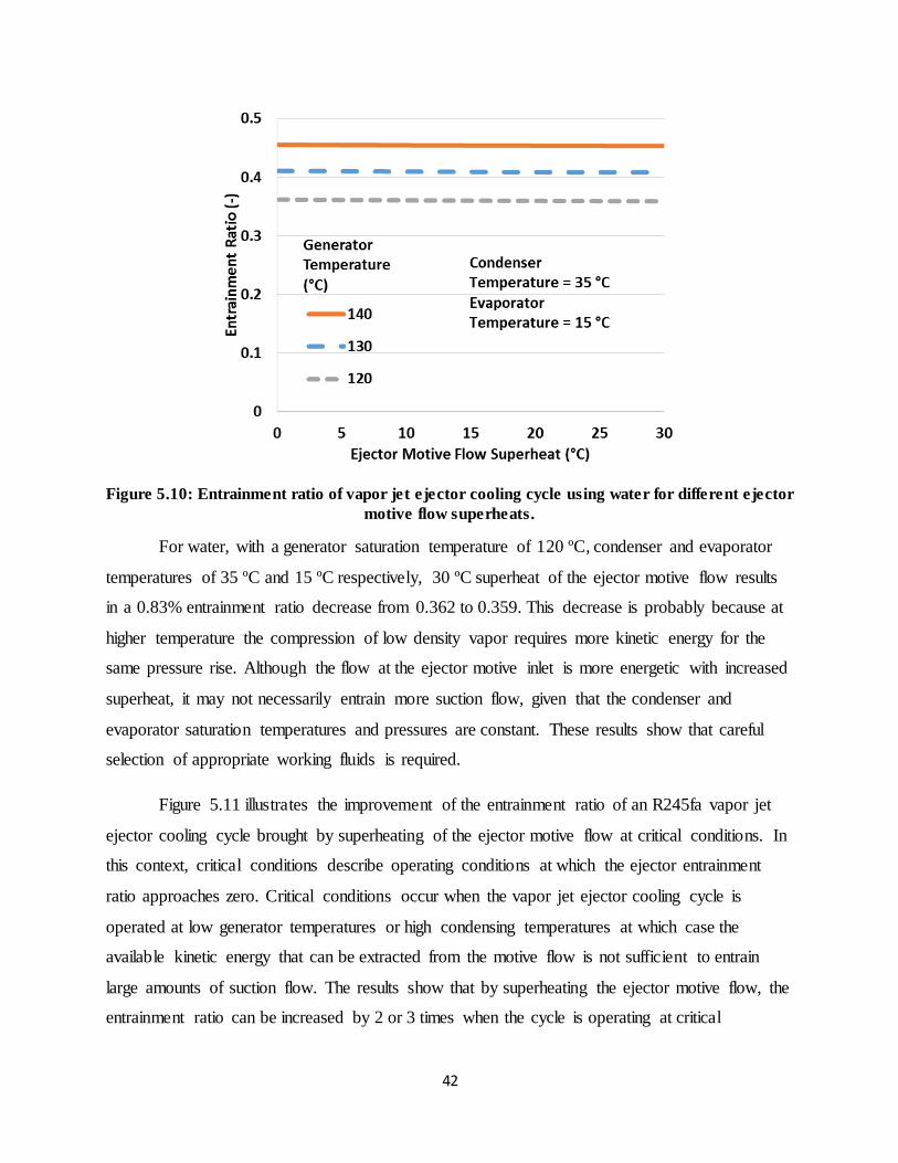
42
Figure 5.10: Entrainment ratio of vapor jet ejector cooling cycle using water for different ejector
motive flow superheats.
For water, with a generator saturation temperature of 120 ºC, condenser and evaporator
temperatures of 35 ºC and 15 ºC respectively, 30 ºC superheat of the ejector motive flow results
in a 0.83% entrainment ratio decrease from 0.362 to 0.359. This decrease is probably because at
higher temperature the compression of low density vapor requires more kinetic energy for the
same pressure rise. Although the flow at the ejector motive inlet is more energetic with increased
superheat, it may not necessarily entrain more suction flow, given that the condenser and
evaporator saturation temperatures and pressures are constant. These results show that careful
selection of appropriate working fluids is required.
Figure 5.11 illustrates the improvement of the entrainment ratio of an R245fa vapor jet
ejector cooling cycle brought by superheating of the ejector motive flow at critical conditions. In
this context, critical conditions describe operating conditions at which the ejector entrainment
ratio approaches zero. Critical conditions occur when the vapor jet ejector cooling cycle is
operated at low generator temperatures or high condensing temperatures at which case the
available kinetic energy that can be extracted from the motive flow is not sufficient to entrain
large amounts of suction flow. The results show that by superheating the ejector motive flow, the
entrainment ratio can be increased by 2 or 3 times when the cycle is operating at critical
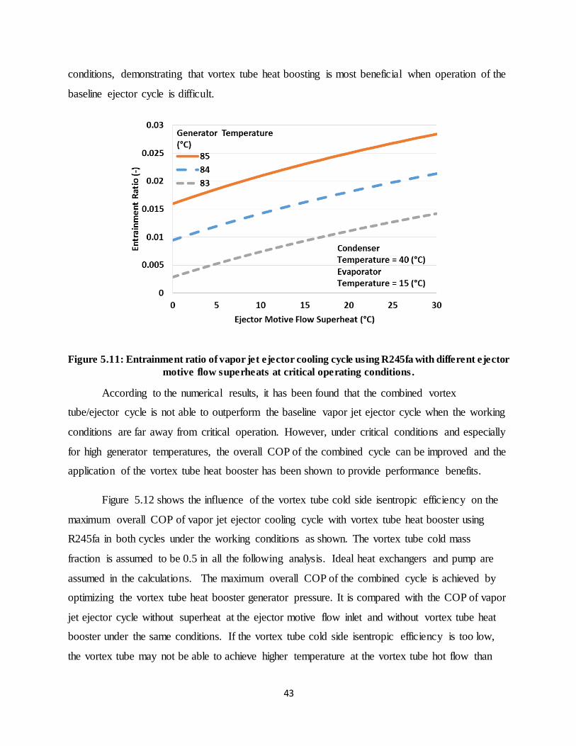
43
conditions, demonstrating that vortex tube heat boosting is most beneficial when operation of the
baseline ejector cycle is difficult.
Figure 5.11: Entrainment ratio of vapor jet ejector cooling cycle using R245fa with different ejector
motive flow superheats at critical operating conditions.
According to the numerical results, it has been found that the combined vortex
tube/ejector cycle is not able to outperform the baseline vapor jet ejector cycle when the working
conditions are far away from critical operation. However, under critical conditions and especially
for high generator temperatures, the overall COP of the combined cycle can be improved and the
application of the vortex tube heat booster has been shown to provide performance benefits.
Figure 5.12 shows the influence of the vortex tube cold side isentropic efficiency on the
maximum overall COP of vapor jet ejector cooling cycle with vortex tube heat booster using
R245fa in both cycles under the working conditions as shown. The vortex tube cold mass
fraction is assumed to be 0.5 in all the following analysis. Ideal heat exchangers and pump are
assumed in the calculations. The maximum overall COP of the combined cycle is achieved by
optimizing the vortex tube heat booster generator pressure. It is compared with the COP of vapor
jet ejector cycle without superheat at the ejector motive flow inlet and without vortex tube heat
booster under the same conditions. If the vortex tube cold side isentropic efficiency is too low,
the vortex tube may not be able to achieve higher temperature at the vortex tube hot flow than
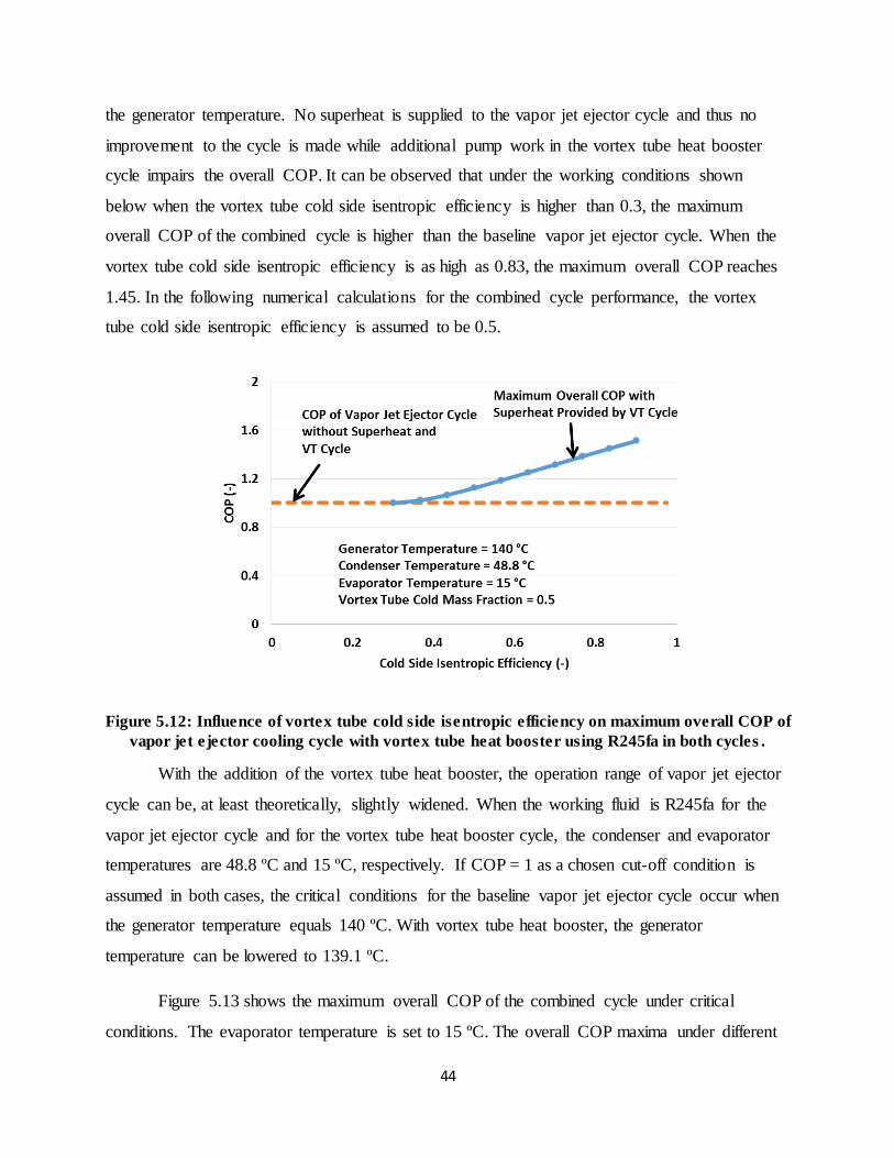
44
the generator temperature. No superheat is supplied to the vapor jet ejector cycle and thus no
improvement to the cycle is made while additional pump work in the vortex tube heat booster
cycle impairs the overall COP. It can be observed that under the working conditions shown
below when the vortex tube cold side isentropic efficiency is higher than 0.3, the maximum
overall COP of the combined cycle is higher than the baseline vapor jet ejector cycle. When the
vortex tube cold side isentropic efficiency is as high as 0.83, the maximum overall COP reaches
1.45. In the following numerical calculations for the combined cycle performance, the vortex
tube cold side isentropic efficiency is assumed to be 0.5.
Figure 5.12: Influence of vortex tube cold side isentropic efficiency on maximum overall COP of
vapor jet ejector cooling cycle with vortex tube heat booster using R245fa in both cycles .
With the addition of the vortex tube heat booster, the operation range of vapor jet ejector
cycle can be, at least theoretically, slightly widened. When the working fluid is R245fa for the
vapor jet ejector cycle and for the vortex tube heat booster cycle, the condenser and evaporator
temperatures are 48.8 ºC and 15 ºC, respectively. If COP = 1 as a chosen cut-off condition is
assumed in both cases, the critical conditions for the baseline vapor jet ejector cycle occur when
the generator temperature equals 140 ºC. With vortex tube heat booster, the generator
temperature can be lowered to 139.1 ºC.
Figure 5.13 shows the maximum overall COP of the combined cycle under critical
conditions. The evaporator temperature is set to 15 ºC. The overall COP maxima under different
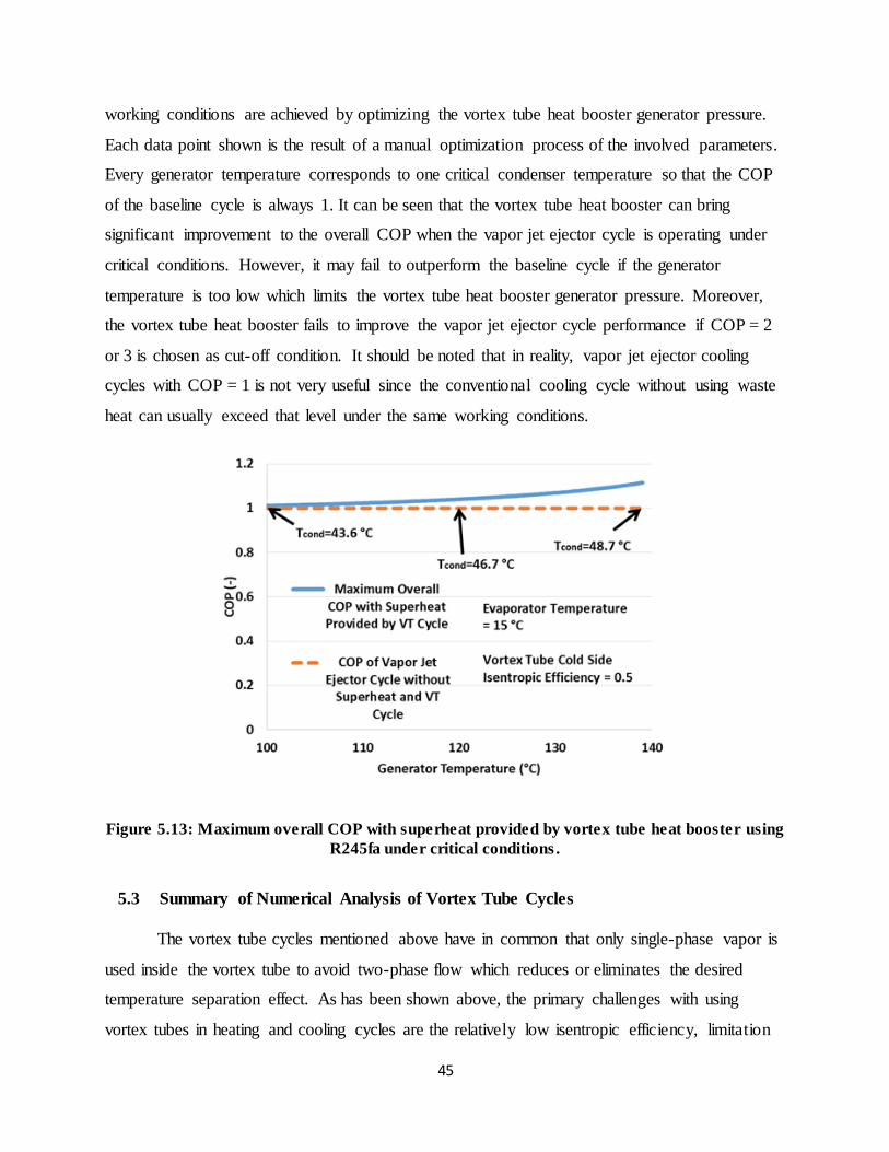
45
working conditions are achieved by optimizing the vortex tube heat booster generator pressure.
Each data point shown is the result of a manual optimization process of the involved parameters.
Every generator temperature corresponds to one critical condenser temperature so that the COP
of the baseline cycle is always 1. It can be seen that the vortex tube heat booster can bring
significant improvement to the overall COP when the vapor jet ejector cycle is operating under
critical conditions. However, it may fail to outperform the baseline cycle if the generator
temperature is too low which limits the vortex tube heat booster generator pressure. Moreover,
the vortex tube heat booster fails to improve the vapor jet ejector cycle performance if COP = 2
or 3 is chosen as cut-off condition. It should be noted that in reality, vapor jet ejector cooling
cycles with COP = 1 is not very useful since the conventional cooling cycle without using waste
heat can usually exceed that level under the same working conditions.
Figure 5.13: Maximum overall COP with superheat provided by vortex tube heat booster using
R245fa under critical conditions .
5.3 Summary of Numerical Analysis of Vortex Tube Cycles
The vortex tube cycles mentioned above have in common that only single-phase vapor is
used inside the vortex tube to avoid two-phase flow which reduces or eliminates the desired
temperature separation effect. As has been shown above, the primary challenges with using
vortex tubes in heating and cooling cycles are the relatively low isentropic efficiency, limitation
46
on the phase of working fluid (that is, only single-phase vapor is used inside the vortex tube) and
the fact that achieving temperatures higher than the vortex tube inlet temperature seems difficult
when refrigerant vapor with non-ideal gas behavior is used. Limitation on the phase of working
fluid restricts the amount of pressure drop and flow that can be used to drive the vortex tube and
create thermal separation, thus improvement to COP brought by the introduction of vortex tube
is small. Suitable working fluids need to be chosen for the vortex tube heat booster cycle, which
should behave like an ideal gas at the low grade heat temperature and can be condensed at
ambient temperature within a reasonable pressure range.
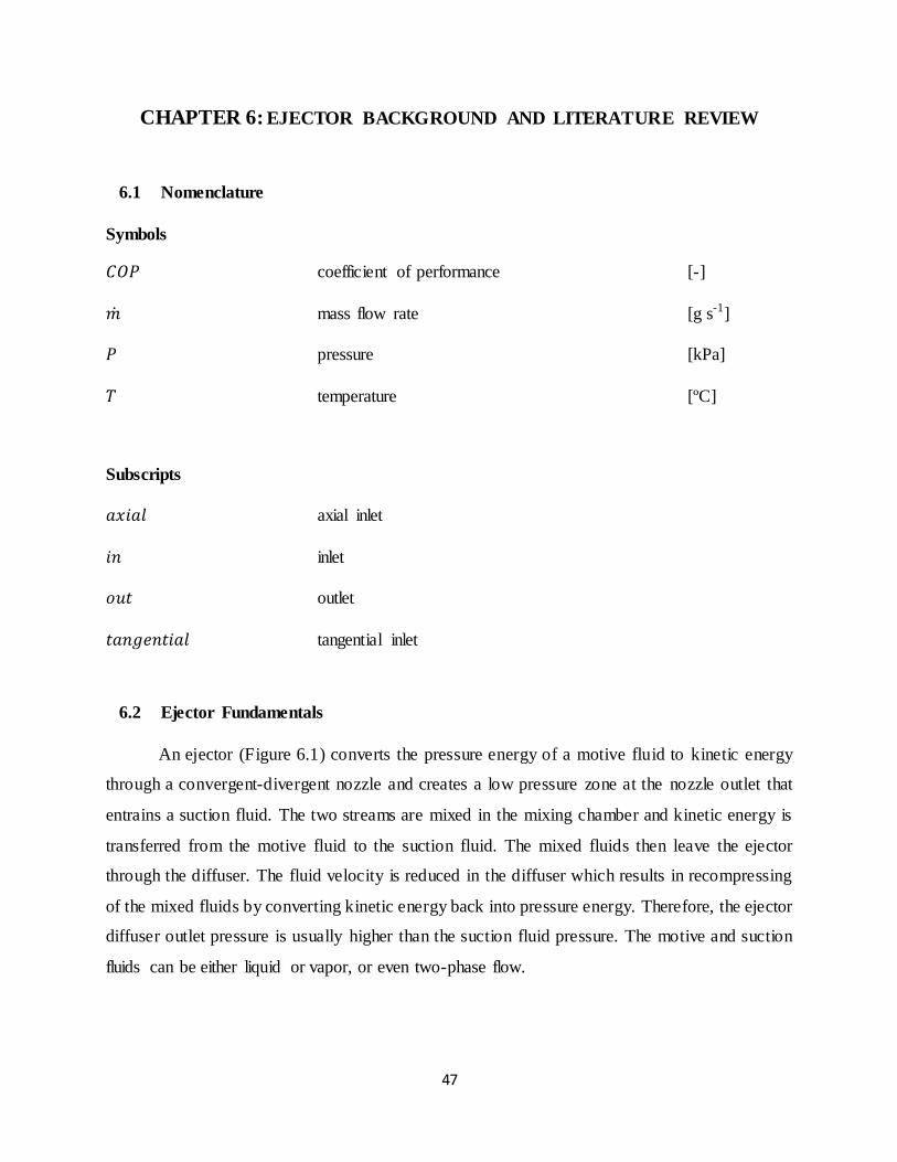
47
CHAPTER 6: EJECTOR BACKGROUND AND LITERATURE REVIEW
6.1 Nomenclature
Symbols
𝐶𝑂𝑃 coefficient of performance [-]
�̇� mass flow rate [g s-1]
𝑃 pressure [kPa]
𝑇 temperature [ºC]
Subscripts
𝑎𝑥𝑖𝑎𝑙 axial inlet
𝑖𝑛 inlet
𝑜𝑢𝑡 outlet
𝑡𝑎𝑛𝑔𝑒𝑛𝑡𝑖𝑎𝑙 tangential inlet
6.2 Ejector Fundamentals
An ejector (Figure 6.1) converts the pressure energy of a motive fluid to kinetic energy
through a convergent-divergent nozzle and creates a low pressure zone at the nozzle outlet that
entrains a suction fluid. The two streams are mixed in the mixing chamber and kinetic energy is
transferred from the motive fluid to the suction fluid. The mixed fluids then leave the ejector
through the diffuser. The fluid velocity is reduced in the diffuser which results in recompressing
of the mixed fluids by converting kinetic energy back into pressure energy. Therefore, the ejector
diffuser outlet pressure is usually higher than the suction fluid pressure. The motive and suction
fluids can be either liquid or vapor, or even two-phase flow.
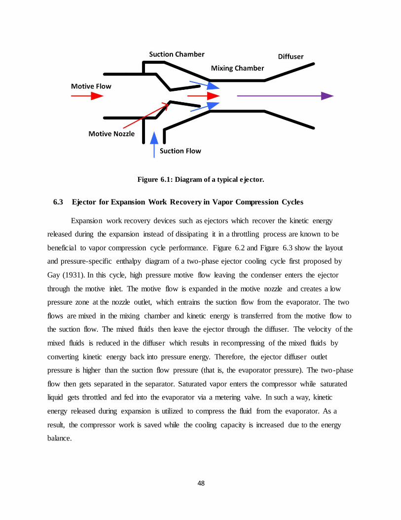
48
Figure 6.1: Diagram of a typical ejector.
6.3 Ejector for Expansion Work Recovery in Vapor Compression Cycles
Expansion work recovery devices such as ejectors which recover the kinetic energy
released during the expansion instead of dissipating it in a throttling process are known to be
beneficial to vapor compression cycle performance. Figure 6.2 and Figure 6.3 show the layout
and pressure-specific enthalpy diagram of a two-phase ejector cooling cycle first proposed by
Gay (1931). In this cycle, high pressure motive flow leaving the condenser enters the ejector
through the motive inlet. The motive flow is expanded in the motive nozzle and creates a low
pressure zone at the nozzle outlet, which entrains the suction flow from the evaporator. The two
flows are mixed in the mixing chamber and kinetic energy is transferred from the motive flow to
the suction flow. The mixed fluids then leave the ejector through the diffuser. The velocity of the
mixed fluids is reduced in the diffuser which results in recompressing of the mixed fluids by
converting kinetic energy back into pressure energy. Therefore, the ejector diffuser outlet
pressure is higher than the suction flow pressure (that is, the evaporator pressure). The two-phase
flow then gets separated in the separator. Saturated vapor enters the compressor while saturated
liquid gets throttled and fed into the evaporator via a metering valve. In such a way, kinetic
energy released during expansion is utilized to compress the fluid from the evaporator. As a
result, the compressor work is saved while the cooling capacity is increased due to the energy
balance.
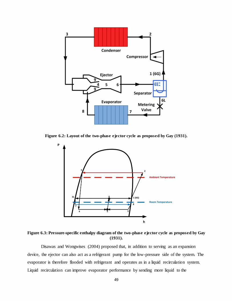
49
Figure 6.2: Layout of the two-phase ejector cycle as proposed by Gay (1931).
Figure 6.3: Pressure-specific enthalpy diagram of the two-phase ejector cycle as proposed by Gay
(1931).
Disawas and Wongwises (2004) proposed that, in addition to serving as an expansion
device, the ejector can also act as a refrigerant pump for the low-pressure side of the system. The
evaporator is therefore flooded with refrigerant and operates as in a liquid recirculation system.
Liquid recirculation can improve evaporator performance by sending more liquid to the
50
evaporator than is actually evaporated so that dryout in the evaporator can be reduced. It can also
improve refrigerant distribution for evaporators with inlet headers by feeding only single-phase
liquid to the inlet headers instead of two-phase refrigerant which often results in non-
homogeneous flow regime. Therefore, liquid recirculation can result in higher evaporation
pressure, and higher system COP compared to a direct expansion cycle (Lawrence and Elbel,
2014).
Many research efforts have been devoted to carbon dioxide transcritical ejector cycles.
Transcritical cycles usually have larger expansion losses caused by throttling process than
subcritical cycles. It is very beneficial to apply ejector to carbon dioxide transcritical cycles due
to the large recovery potential.
Ozaki et al. (2004) carried out an experiment on an automotive air conditioning system
using carbon dioxide as the refrigerant to improve system COP. The experiment showed COP
improvement of 20% over a baseline cycle using a conventional expansion valve.
Banasiak et al. (2012) reported maximum increase in COP of 8% over a baseline cycle
with a conventional expansion valve.
Elbel and Hrnjak (2008) experimentally investigated a transcritical carbon dioxide system
using a refrigerant ejector. They reported that for the test conditions considered the cooling
capacity and COP can be simultaneously improved by up to 8% and 7%, respectively.
Extrapolation was used to determine that the COP could have been improved by as much as 18%
at matched cooling capacities.
Less attention has been given to low-pressure working fluids in the literature for ejector
cooling cycles compared with carbon dioxide due to their lower work recovery potential.
However, ejector cooling cycles using low-pressure refrigerant can still have noticeable
performance improvements.
Early investigation of a two-phase ejector cycle using R134a by Harrell and Kornhauser
(1995) predicted a cooling COP improvement of approximately 23% for a typical refrigerating
cycle and an ideal ejector. An improvement of 12% could be achieved if the ejector performed as
51
well as typical single-phase ejectors. Ejector performance achieved from later ejector tests
corresponded to refrigeration cycle COP improvements ranging from 3.9% to 7.6%.
Lawrence and Elbel (2014) experimentally investigated the performance of an alternate
two-phase ejector cycle in which the pressure lift provided by the ejector was utilized to provide
multiple evaporation temperatures. The working fluids were low-pressure fluids R134a and
R1234yf. The ejector cycle showed maximum COP improvements of 12% with R1234yf and 8%
with R134a when compared to a two evaporation temperature expansion valve cycle. When
compared to a single evaporation temperature expansion valve cycle, the ejector cycle showed
maximum COP improvements of 6% with R1234yf and 5% with R134a.
Disawas and Wongwises (2004) presented experimental data on the performance of a
two-phase ejector refrigeration cycle using R134a which enables the evaporator to operate as in a
liquid-recirculation system. The results showed that the COP of the two-phase ejector cycle is
higher than that of the baseline cycle using expansion valve over the whole range of
experimental conditions. The maximum improvement achieved was about 13% at low heat sink
and heat source temperatures.
6.4 Influence of Working Conditions and Ejector Dimensions on Ejector Cycle
Performance
Ejector cycle performance is usually sensitive to working condition changes which are
common in real world applications. Different working conditions require different ejector
geometries to achieve maximum performance. Slightly different geometries may result in
substantially different COPs under the same conditions. Therefore, it is desirable to introduce an
adjustable feature to the ejector so that ejector cycle performance can be optimized under
different working conditions, which could make ejector technology more suitable for real world
applications (Sumeru et al., 2012).
The ejector motive nozzle throat diameter is one of the key dimensions that affect COP. It
has a direct impact on motive mass flow rate. Other important ejector geometric parameters that
affect ejector efficiency and COP include motive nozzle position, constant area diameter of the
mixing chamber and suction chamber converging angle. Additional information can be found in
Sarkar (2012). One way to adjust the motive nozzle throat diameter in order to optimize ejector
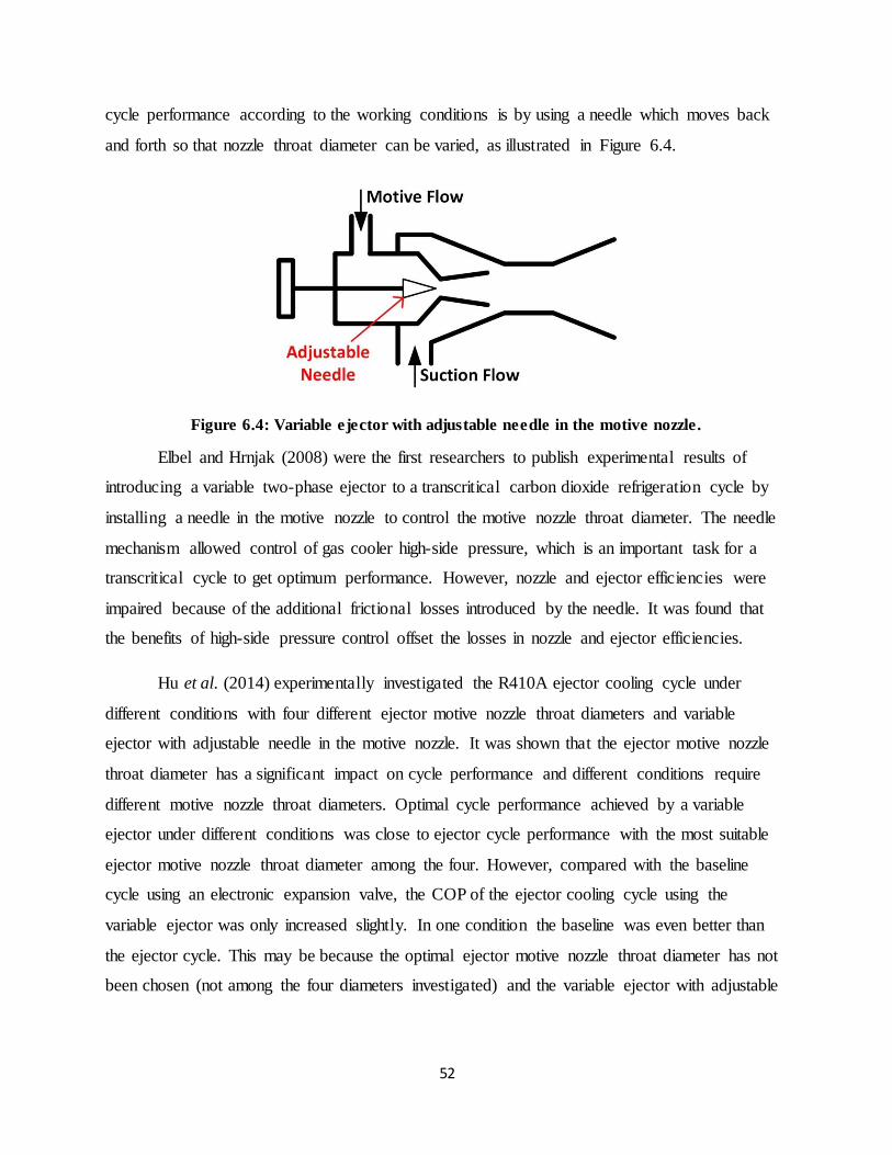
52
cycle performance according to the working conditions is by using a needle which moves back
and forth so that nozzle throat diameter can be varied, as illustrated in Figure 6.4.
Figure 6.4: Variable ejector with adjustable needle in the motive nozzle.
Elbel and Hrnjak (2008) were the first researchers to publish experimental results of
introducing a variable two-phase ejector to a transcritical carbon dioxide refrigeration cycle by
installing a needle in the motive nozzle to control the motive nozzle throat diameter. The needle
mechanism allowed control of gas cooler high-side pressure, which is an important task for a
transcritical cycle to get optimum performance. However, nozzle and ejector efficiencies were
impaired because of the additional frictional losses introduced by the needle. It was found that
the benefits of high-side pressure control offset the losses in nozzle and ejector efficiencies.
Hu et al. (2014) experimentally investigated the R410A ejector cooling cycle under
different conditions with four different ejector motive nozzle throat diameters and variable
ejector with adjustable needle in the motive nozzle. It was shown that the ejector motive nozzle
throat diameter has a significant impact on cycle performance and different conditions require
different motive nozzle throat diameters. Optimal cycle performance achieved by a variable
ejector under different conditions was close to ejector cycle performance with the most suitable
ejector motive nozzle throat diameter among the four. However, compared with the baseline
cycle using an electronic expansion valve, the COP of the ejector cooling cycle using the
variable ejector was only increased slightly. In one condition the baseline was even better than
the ejector cycle. This may be because the optimal ejector motive nozzle throat diameter has not
been chosen (not among the four diameters investigated) and the variable ejector with adjustable
53
needle has lower nozzle and ejector efficiencies because of the additional frictional losses
incurred by the needle.
6.5 Summary of Literature Review
An ejector can be used as an expansion work recovery device in either subcritical or
transcritical vapor compression cycles. It can bring noticeable cycle performance improvement
by utilizing the kinetic energy released during the pressure reduction to compress the fluid from
the evaporator so that the compressor work is saved and the cooling capacity is increased. It can
also be used to send more liquid to the evaporator than is actually evaporated so that evaporator
performance can be enhanced and thus the COP is improved.
A variable geometry ejector with adjustable needle in the motive nozzle can optimize
ejector cycle performance under different conditions, but this design is complicated and costly,
and more frictional losses are incurred because of the additional surface area introduced which
results in lower nozzle and ejector efficiencies. This provides motivation to develop a new
technology to control the motive nozzle restrictiveness.
54
CHAPTER 7: NEW VORTEX CONTROL POSSIBLY APPLICABLE TO
EJECTOR REFRIGERATION CYCLES
In this thesis, a novel control mechanism for the restrictiveness of a two-phase nozzle has
been presented, which can possibly be applied to the control of ejector cooling cycles. It utilizes
an adjustable vortex at the nozzle inlet to control the nozzle restrictiveness on the low vapor
quality flow expanded in the nozzle without changing the physical dimensions of the nozzle
geometry. The ejector and nozzle which employ this vortex control mechanism are called vortex
ejector and vortex nozzle in this thesis. At least one control valve is needed for the
implementation of this two-phase nozzle restrictiveness control mechanism. This new control
mechanism has the advantages of being simple, possibly less expensive, and can potentially
avoid the additional frictional losses in previously proposed nozzle restrictiveness control
mechanisms. Controlling the ejector motive nozzle restrictiveness by adjusting the vortex
strength can be very useful for the future application of ejector cooling cycles in mobile or
stationary systems that experience wide range of operating conditions.
7.1 Introduction to Vortex Ejector and Vortex Control
A vortex ejector differs from a conventional ejector in that an adjustable vortex is
generated at the ejector motive inlet, as is shown in Figure 7.1. The motive inlet vortex can be
created by injecting part of the motive flow tangentially. After injection the tangential flow will
be mixed with the axial motive flow. The total mass flow rate passing through the vortex motive
nozzle is equal to the sum of mass flow rates entering through the motive nozzle’s axial and
tangential flow inlets. The ejector cooling cycle shown in Figure 7.2 that uses a vortex ejector is
almost the same as the conventional ejector cooling cycle in Figure 6.2. The only difference is
that the flow at the condenser outlet of the vortex ejector cooling cycle is separated into two
streams. One stream enters the vortex ejector through the motive flow tangential inlet and
another enters through the motive flow axial inlet. In such a way, a vortex is created at the
ejector motive inlet. The ratio of mass flow rates through the two inlets can be adjusted by a
valve installed at the motive flow tangential inlet, thereby changing the vortex strength. The
pressure drop across the control valve is usually small. It can be assumed that the thermodynamic
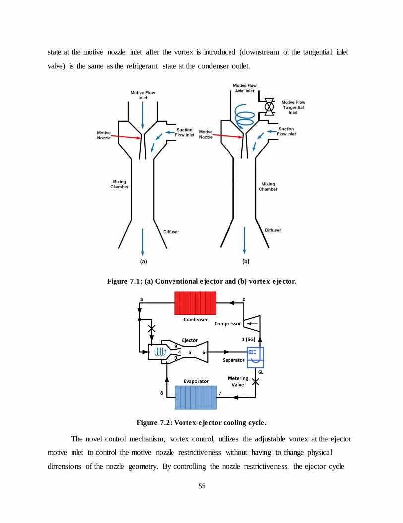
55
state at the motive nozzle inlet after the vortex is introduced (downstream of the tangential inlet
valve) is the same as the refrigerant state at the condenser outlet.
Figure 7.1: (a) Conventional ejector and (b) vortex ejector.
Figure 7.2: Vortex ejector cooling cycle.
The novel control mechanism, vortex control, utilizes the adjustable vortex at the ejector
motive inlet to control the motive nozzle restrictiveness without having to change physical
dimensions of the nozzle geometry. By controlling the nozzle restrictiveness, the ejector cycle
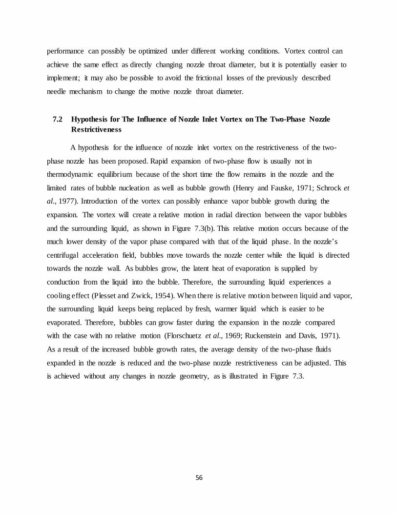
56
performance can possibly be optimized under different working conditions. Vortex control can
achieve the same effect as directly changing nozzle throat diameter, but it is potentially easier to
implement; it may also be possible to avoid the frictional losses of the previously described
needle mechanism to change the motive nozzle throat diameter.
7.2 Hypothesis for The Influence of Nozzle Inlet Vortex on The Two-Phase Nozzle
Restrictiveness
A hypothesis for the influence of nozzle inlet vortex on the restrictiveness of the two-
phase nozzle has been proposed. Rapid expansion of two-phase flow is usually not in
thermodynamic equilibrium because of the short time the flow remains in the nozzle and the
limited rates of bubble nucleation as well as bubble growth (Henry and Fauske, 1971; Schrock et
al., 1977). Introduction of the vortex can possibly enhance vapor bubble growth during the
expansion. The vortex will create a relative motion in radial direction between the vapor bubbles
and the surrounding liquid, as shown in Figure 7.3(b). This relative motion occurs because of the
much lower density of the vapor phase compared with that of the liquid phase. In the nozzle’s
centrifugal acceleration field, bubbles move towards the nozzle center while the liquid is directed
towards the nozzle wall. As bubbles grow, the latent heat of evaporation is supplied by
conduction from the liquid into the bubble. Therefore, the surrounding liquid experiences a
cooling effect (Plesset and Zwick, 1954). When there is relative motion between liquid and vapor,
the surrounding liquid keeps being replaced by fresh, warmer liquid which is easier to be
evaporated. Therefore, bubbles can grow faster during the expansion in the nozzle compared
with the case with no relative motion (Florschuetz et al., 1969; Ruckenstein and Davis, 1971).
As a result of the increased bubble growth rates, the average density of the two-phase fluids
expanded in the nozzle is reduced and the two-phase nozzle restrictiveness can be adjusted. This
is achieved without any changes in nozzle geometry, as is illustrated in Figure 7.3.
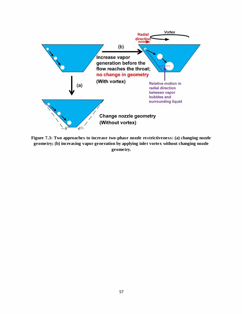
57
Figure 7.3: Two approaches to increase two-phase nozzle restrictiveness: (a) changing nozzle
geometry; (b) increasing vapor generation by applying inlet vortex without changing nozzle
geometry.
58
CHAPTER 8: EXPERIMENTAL FACILITY AND METHODS FOR
INVESTIGATION OF THE INFLUENCE OF INLET VORTEX ON NOZZLE
RESTRICTIVENESS
8.1 Vortex Nozzle Design
In order to investigate the influence of inlet vortex on nozzle restrictiveness and visualize
the two-phase flow expanded in the convergent-divergent nozzle, a transparent nozzle with
controllable vortex at the nozzle inlet has been designed and manufactured, as is shown in Figure
8.1. Important dimensions of the vortex nozzle have been summarized in Table 8.1 and these
dimensions are shown with corresponding letters in Figure 8.1. It should be noted that the nozzle
is only part of a vortex ejector. Experimental investigation of vortex ejectors in ejector cooling
systems will be conducted in the future. The vortex nozzle is composed of three components: a
tee part made of brass, a sleeve and a convergent-divergent nozzle, as shown in Figure 8.2, both
made of an optically clear resin called Waterclear Ultra 10122 from SOMOS and manufactured
by Stereo Lithography Apparatus (SLA) from 3D SYSTEMS.
Figure 8.1: Vortex nozzle composed of tee, sleeve and convergent-divergent nozzle.
59
Table 8.1: Vortex nozzle geometric parameters.
(a) Nozzle inlet diameter (mm) 15
(b) Nozzle throat diameter (mm) 1.0
(c) Nozzle outlet diameter (mm) 1.7
(d) Nozzle convergent part length
(mm)
9.9
(e) Nozzle divergent part length
(mm)
40
(f) Tangential inlet inner diameter
(mm)
2.0
(g) Vortex decay distance (mm) 138
Figure 8.2: 3D printed transparent convergent-divergent nozzle.
The tee part serves as a vortex generator. The tangential inlet on the tee allows flow to be
injected tangentially and mix with the axial flow, thus creating a vortex. The tee and the nozzle
are joined by an NPT thread and sealed by epoxy adhesive. The other NPT thread on the nozzle
60
is for connection with the visualization chamber. The sleeve is designed to provide a smooth
transition between the tee part and the nozzle. There is no gap between the tee part and the
nozzle so that no additional disturbance is introduced to the flow. The inner diameter of the
sleeve is the same as that of the nozzle entrance. There is a tangential inlet on the sleeve.
Tangential inlet on the tee and tangential inlet on the sleeve are coaxial and have the same inner
diameter. For visualization purpose, the flow needs to travel a long distance from the tangential
inlet to the starting point of the convergent part of the nozzle. This distance is called vortex
decay distance, as shown in Figure 8.1 with the letter ‘g’. Because of the fluid viscosity and
turbulence, vortex strength will decay over this distance. In future real world applications, such a
long distance between the tangential inlet and nozzle convergent part may not be necessary.
Therefore, it is desirable to find out the real vortex strength at the starting point of the nozzle
convergent part so that the true relation between the nozzle inlet vortex strength (at the starting
point of the convergent part) and the nozzle restrictiveness can be determined. The sleeve also
makes sure that the swirling flow travels and decays in a pipe with constant surface properties
before it reaches the convergent part of the nozzle, which simplifies future calculation of vortex
decay over the vortex decay distance.
8.2 Experimental Setup and Its Components
The layout of the experimental facility for the vortex nozzle tests is shown in Figure 8.3.
A pumped-refrigerant- loop was used for adjustment of test conditions to investigate the influence
of inlet vortex on the two-phase flow expanded in the convergent-divergent nozzle. The working
fluid was R134a. A visualization chamber was built from clear PVC pipe. The temperature
readings were all obtained from ungrounded Type-T immersion thermocouples. The measured
temperatures are regarded as total temperatures. Absolute pressures were read by piezo-electric
pressure transducers. Pressures and temperatures at the axial and tangential inlets of the nozzle
were measured. The axial inlet pressure is assumed to be the nozzle inlet pressure 𝑃𝑖𝑛. The
pressure at the nozzle outlet 𝑃𝑜𝑢𝑡 was measured as well. The total mass flow rate �̇� 𝑡𝑜𝑡𝑎𝑙 and the
nozzle axial inlet mass flow rate �̇�𝑎𝑥𝑖𝑎𝑙 were measured by Coriolis-type mass flow meters. The
nozzle’s tangential inlet mass flow rate �̇� 𝑡𝑎𝑛𝑔𝑒𝑛𝑡𝑖𝑎𝑙 can be calculated by subtracting the nozzle
axial inlet mass flow rate from the total mass flow rate. The ratio of the nozzle tangential inlet
mass flow rate to the total mass flow rate was adjusted by two valves. The larger the ratio is, the
61
large the vortex strength is for the same total mass flow rate. In this thesis, the vortex strength is
defined as the ratio of the nozzle tangential inlet mass flow rate to the total mass flow rate, which
can be expressed as shown in Equation 8.1:
𝑉𝑜𝑟𝑡𝑒𝑥 𝑠𝑡𝑟𝑒𝑛𝑔𝑡ℎ =�̇�𝑡𝑎𝑛𝑔𝑒𝑛𝑡𝑖𝑎𝑙
�̇�𝑡𝑜𝑡𝑎𝑙 (8.1)
Figure 8.3: Experimental facility for investigation of vortex influence on nozzle restrictiveness.
It should be noted that in order to use the full range of vortex control from zero vortex to
maximum vortex, two valves are installed in the test rig at both the nozzle’s axial and tangential
inlets. However, in real world applications, one valve should be sufficient to achieve nozzle
restrictiveness control over a suitable range.
62
8.3 Test Methods and Conditions
Different nozzle inlet pressures were achieved by adjusting the heating water temperature
and pump speed which determine the saturation pressure of the refrigerant in the heater. The
differences between the vortex nozzle axial inlet pressures and tangential inlet pressures were
generally within 10 kPa. The temperature differences between the axial and tangential inlets of
the nozzle were kept within 0.5 ºC. When the axial or tangential inlet mass flow rate was close to
zero, heat losses in the tubes had significant cooling effect on the flow even with insulation. For
example, when the nozzle inlet pressure was 926 kPa while the total mass flow rate and the axial
inlet mass flow rate were 13.1 g s-1 and 2.6 g s-1, respectively, the tangential inlet temperature
was kept at 36.4 ºC while the axial inlet temperature was only 33.0 ºC. Therefore it is difficult to
keep the same temperatures at both nozzle inlets when one of the inlet mass flow rates is close to
zero and the data obtained in those cases are not shown in the results in Chapter 9. However,
when one of the two inlets is fully closed, there is no such problem and only the conditions at the
open inlet need to be controlled. The nozzle outlet pressure can be adjusted by a valve installed
downstream of the nozzle. For all experimental results shown in this thesis, the liquid flow at the
nozzle inlet was subcooled by approximately 0.5 ºC. Admittedly, the calculated subcooling is
close to the uncertainty of thermocouple reading and it is imprudent to claim the inlet is
subcooled solely based on the thermocouple readings. The sight glass installed at the nozzle inlet
allows for visual confirmation that no bubbles are present at the nozzle inlet, which provides a
double check for inlet subcooling.
Data were all collected at steady-state; once steady-state conditions were reached in the
system, data were collected for 4 consecutive minutes, and the data for each measurement were
averaged over the data collection period. The variation range of the controlled variables in the
vortex nozzle experiments reported in Chapter 9 is summarized in Table 8.2.
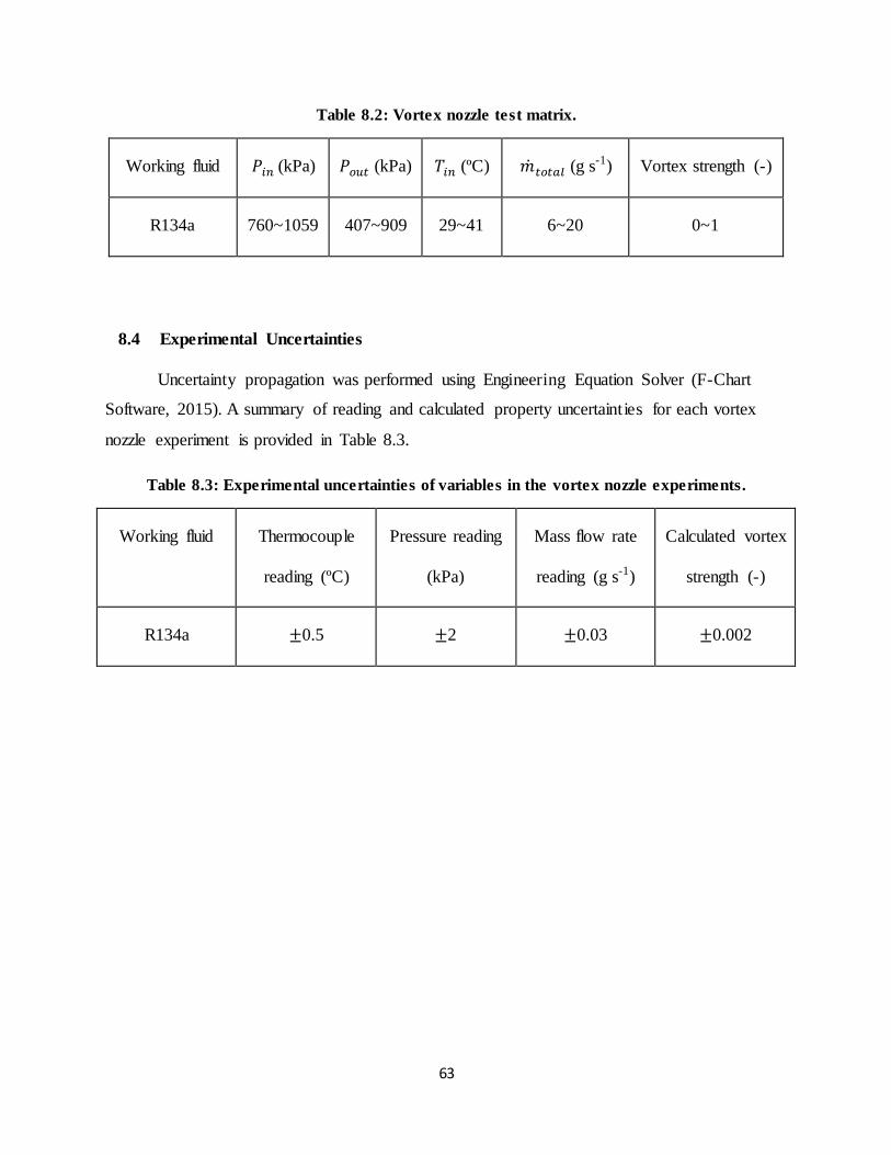
63
Table 8.2: Vortex nozzle test matrix.
Working fluid 𝑃𝑖𝑛 (kPa) 𝑃𝑜𝑢𝑡 (kPa) 𝑇𝑖𝑛 (ºC) �̇�𝑡𝑜𝑡𝑎𝑙 (g s-1) Vortex strength (-)
R134a 760~1059 407~909 29~41 6~20 0~1
8.4 Experimental Uncertainties
Uncertainty propagation was performed using Engineering Equation Solver (F-Chart
Software, 2015). A summary of reading and calculated property uncertainties for each vortex
nozzle experiment is provided in Table 8.3.
Table 8.3: Experimental uncertainties of variables in the vortex nozzle experiments.
Working fluid Thermocouple
reading (ºC)
Pressure reading
(kPa)
Mass flow rate
reading (g s-1)
Calculated vortex
strength (-)
R134a ±0.5 ±2 ±0.03 ±0.002
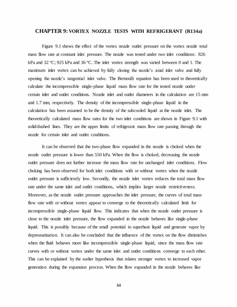
64
CHAPTER 9: VORTEX NOZZLE TESTS WITH REFRIGERANT (R134a)
Figure 9.1 shows the effect of the vortex nozzle outlet pressure on the vortex nozzle total
mass flow rate at constant inlet pressure. The nozzle was tested under two inlet conditions: 826
kPa and 32 ºC; 925 kPa and 36 ºC. The inlet vortex strength was varied between 0 and 1. The
maximum inlet vortex can be achieved by fully closing the nozzle’s axial inlet valve and fully
opening the nozzle’s tangential inlet valve. The Bernoulli equation has been used to theoretically
calculate the incompressible single-phase liquid mass flow rate for the tested nozzle under
certain inlet and outlet conditions. Nozzle inlet and outlet diameters in the calculation are 15 mm
and 1.7 mm, respectively. The density of the incompressible single-phase liquid in the
calculation has been assumed to be the density of the subcooled liquid at the nozzle inlet. The
theoretically calculated mass flow rates for the two inlet conditions are shown in Figure 9.1 with
solid/dashed lines. They are the upper limits of refrigerant mass flow rate passing through the
nozzle for certain inlet and outlet conditions.
It can be observed that the two-phase flow expanded in the nozzle is choked when the
nozzle outlet pressure is lower than 550 kPa. When the flow is choked, decreasing the nozzle
outlet pressure does not further increase the mass flow rate for unchanged inlet conditions. Flow
choking has been observed for both inlet conditions with or without vortex when the nozzle
outlet pressure is sufficiently low. Secondly, the nozzle inlet vortex reduces the total mass flow
rate under the same inlet and outlet conditions, which implies larger nozzle restrictiveness.
Moreover, as the nozzle outlet pressure approaches the inlet pressure, the curves of total mass
flow rate with or without vortex appear to converge to the theoretically calculated limit for
incompressible single-phase liquid flow. This indicates that when the nozzle outlet pressure is
close to the nozzle inlet pressure, the flow expanded in the nozzle behaves like single-phase
liquid. This is possibly because of the small potential to superheat liquid and generate vapor by
depressurization. It can also be concluded that the influence of the vortex on the flow diminishes
when the fluid behaves more like incompressible single-phase liquid, since the mass flow rate
curves with or without vortex under the same inlet and outlet conditions converge to each other.
This can be explained by the earlier hypothesis that relates stronger vortex to increased vapor
generation during the expansion process. When the flow expanded in the nozzle behaves like
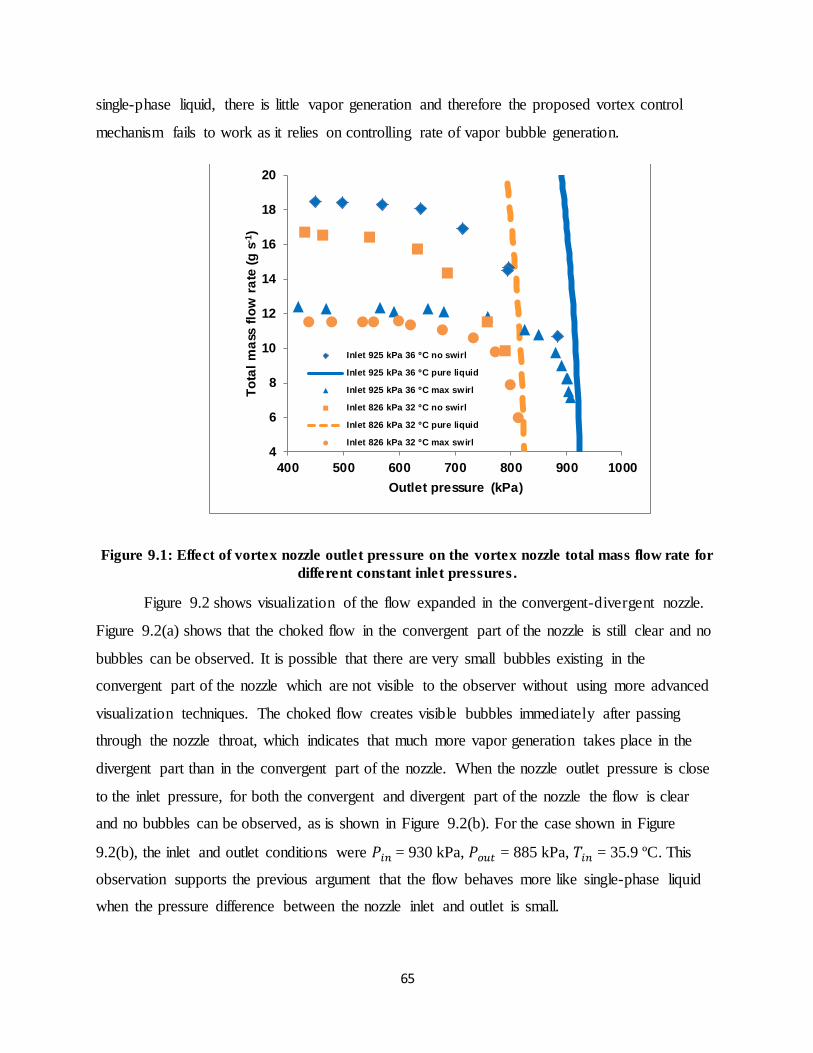
65
single-phase liquid, there is little vapor generation and therefore the proposed vortex control
mechanism fails to work as it relies on controlling rate of vapor bubble generation.
Figure 9.1: Effect of vortex nozzle outlet pressure on the vortex nozzle total mass flow rate for
different constant inlet pressures .
Figure 9.2 shows visualization of the flow expanded in the convergent-divergent nozzle.
Figure 9.2(a) shows that the choked flow in the convergent part of the nozzle is still clear and no
bubbles can be observed. It is possible that there are very small bubbles existing in the
convergent part of the nozzle which are not visible to the observer without using more advanced
visualization techniques. The choked flow creates visible bubbles immediately after passing
through the nozzle throat, which indicates that much more vapor generation takes place in the
divergent part than in the convergent part of the nozzle. When the nozzle outlet pressure is close
to the inlet pressure, for both the convergent and divergent part of the nozzle the flow is clear
and no bubbles can be observed, as is shown in Figure 9.2(b). For the case shown in Figure
9.2(b), the inlet and outlet conditions were 𝑃𝑖𝑛 = 930 kPa, 𝑃𝑜𝑢𝑡 = 885 kPa, 𝑇𝑖𝑛 = 35.9 ºC. This
observation supports the previous argument that the flow behaves more like single-phase liquid
when the pressure difference between the nozzle inlet and outlet is small.
4
6
8
10
12
14
16
18
20
400 500 600 700 800 900 1000
To
tal
ma
ss f
low
ra
te (g
s-1
)
Outlet pressure (kPa)
Inlet 925 kPa 36 ºC no swirl
Inlet 925 kPa 36 ºC pure liquid
Inlet 925 kPa 36 ºC max swirl
Inlet 826 kPa 32 ºC no swirl
Inlet 826 kPa 32 ºC pure liquid
Inlet 826 kPa 32 ºC max swirl
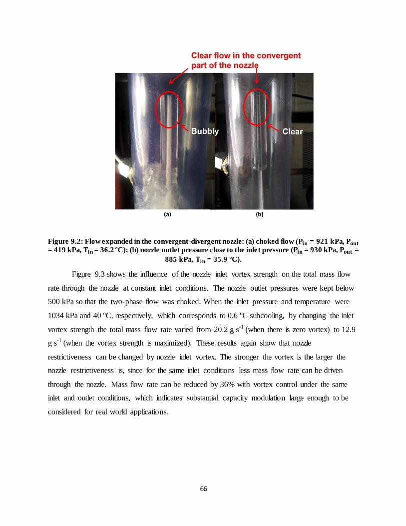
66
Figure 9.2: Flow expanded in the convergent-divergent nozzle: (a) choked flow (𝐏𝐢𝐧 = 921 kPa, 𝐏𝐨𝐮𝐭
= 419 kPa, 𝐓𝐢𝐧 = 36.2 ºC); (b) nozzle outlet pressure close to the inlet pressure (𝐏𝐢𝐧 = 930 kPa, 𝐏𝐨𝐮𝐭 =
885 kPa, 𝐓𝐢𝐧 = 35.9 ºC).
Figure 9.3 shows the influence of the nozzle inlet vortex strength on the total mass flow
rate through the nozzle at constant inlet conditions. The nozzle outlet pressures were kept below
500 kPa so that the two-phase flow was choked. When the inlet pressure and temperature were
1034 kPa and 40 ºC, respectively, which corresponds to 0.6 ºC subcooling, by changing the inlet
vortex strength the total mass flow rate varied from 20.2 g s-1 (when there is zero vortex) to 12.9
g s-1 (when the vortex strength is maximized). These results again show that nozzle
restrictiveness can be changed by nozzle inlet vortex. The stronger the vortex is the larger the
nozzle restrictiveness is, since for the same inlet conditions less mass flow rate can be driven
through the nozzle. Mass flow rate can be reduced by 36% with vortex control under the same
inlet and outlet conditions, which indicates substantial capacity modulation large enough to be
considered for real world applications.
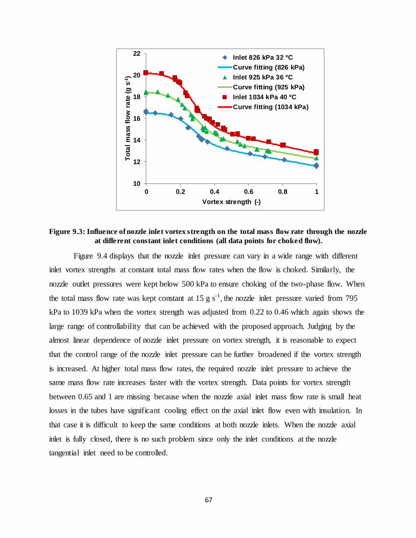
67
Figure 9.3: Influence of nozzle inlet vortex strength on the total mass flow rate through the nozzle
at different constant inlet conditions (all data points for choked flow).
Figure 9.4 displays that the nozzle inlet pressure can vary in a wide range with different
inlet vortex strengths at constant total mass flow rates when the flow is choked. Similarly, the
nozzle outlet pressures were kept below 500 kPa to ensure choking of the two-phase flow. When
the total mass flow rate was kept constant at 15 g s-1, the nozzle inlet pressure varied from 795
kPa to 1039 kPa when the vortex strength was adjusted from 0.22 to 0.46 which again shows the
large range of controllability that can be achieved with the proposed approach. Judging by the
almost linear dependence of nozzle inlet pressure on vortex strength, it is reasonable to expect
that the control range of the nozzle inlet pressure can be further broadened if the vortex strength
is increased. At higher total mass flow rates, the required nozzle inlet pressure to achieve the
same mass flow rate increases faster with the vortex strength. Data points for vortex strength
between 0.65 and 1 are missing because when the nozzle axial inlet mass flow rate is small heat
losses in the tubes have significant cooling effect on the axial inlet flow even with insulation. In
that case it is difficult to keep the same conditions at both nozzle inlets. When the nozzle axial
inlet is fully closed, there is no such problem since only the inlet conditions at the nozzle
tangential inlet need to be controlled.
10
12
14
16
18
20
22
0 0.2 0.4 0.6 0.8 1
To
tal
ma
ss f
low
ra
te (g
s-1
)
Vortex strength (-)
Inlet 826 kPa 32 ºC
Curve fitting (826 kPa)
Inlet 925 kPa 36 ºC
Curve fitting (925 kPa)
Inlet 1034 kPa 40 ºC
Curve fitting (1034 kPa)
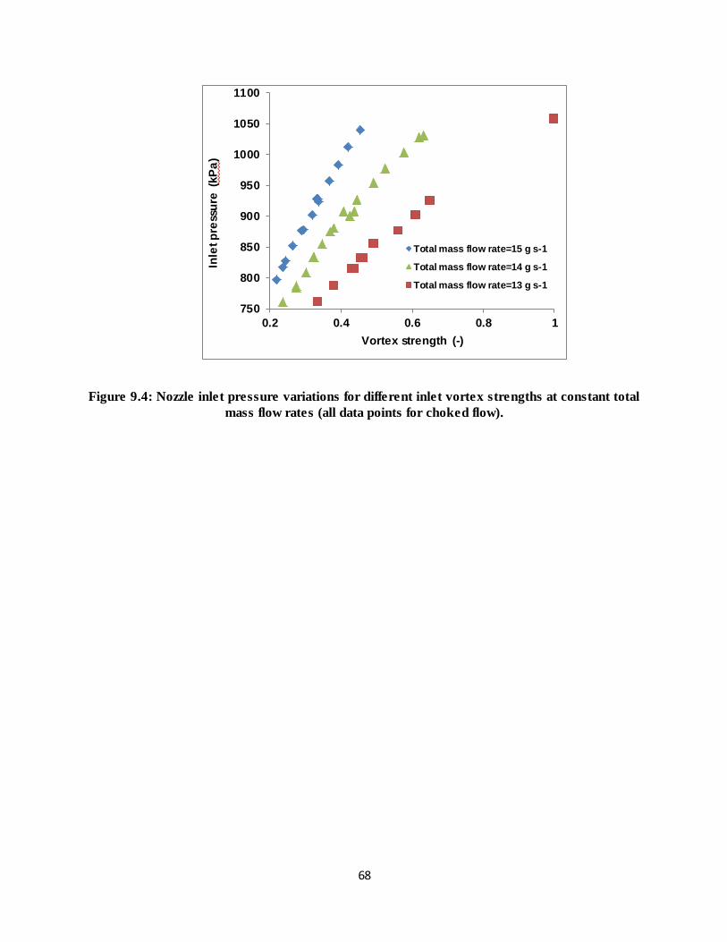
68
Figure 9.4: Nozzle inlet pressure variations for different inlet vortex strengths at constant total
mass flow rates (all data points for choked flow).
750
800
850
900
950
1000
1050
1100
0.2 0.4 0.6 0.8 1
Inle
t p
ress
ure
(kP
a)
Vortex strength (-)
Total mass flow rate=15 g s-1
Total mass flow rate=14 g s-1
Total mass flow rate=13 g s-1
69
CHAPTER 10: CONCLUSIONS AND FUTURE WORK
The vortex tube designed primarily for applications with compressed air is utilized in this
study to investigate the potential of using vortex tube expansion in heating and cooling cycles.
Suitable operating conditions for vortex tube have been identified and actual work recovery
effects have been demonstrated experimentally for both air and refrigerants. The results show
that the vortex tube is capable of producing temperature separation with conventional refrigerant.
The cold end temperature is found to be lower than the isenthalpic expansion temperature which
shows the potential to recover work. Non-ideal gas behavior of refrigerant vapor is believed to be
the reason why the hot end temperature of vortex tube in most cases is lower than the inlet
temperature when using refrigerant. Heating and cooling cycles have been proposed based on the
knowledge of suitable operating conditions for vortex tubes and numerical results of the cycle
performance have been provided. The state point analysis of the vortex tube cooling cycle with
different refrigerants shows rather small improvements on the order of 0.1% for COP for the
conditions considered. With reasonably high vortex tube efficiency and low grade heat available
for free, the vortex tube heat booster cycle can outperform liquid circulating cycles using electric
resistance heat in terms of COP. Major challenges are seen in low isentropic efficiency, necessity
of the working fluid to be single-phase vapor, sufficient temperature raise at the hot end, and
utilization of working fluids with strong non-ideal gas like behavior. Research on the topic is
ongoing, and will include other areas of interest such as the Brayton air cycle or the Claude cycle
used in cryogenic applications where vortex tubes can potentially help more due to the more
ideal gas like behavior of the working fluids used.
A new nozzle restrictiveness control mechanism called vortex control has been proposed
and verified. The approach seems suitable to be applied for the purpose of capacity modulation
for two-phase ejector in vapor compression cycles, which is very relevant for real world
applications. This control mechanism is simple, possibly inexpensive and can potentially yield
better efficiencies than other approaches that attempt to control nozzle flow rates. A hypothesis
for the influence of nozzle inlet vortex on the restrictiveness of the two-phase nozzle has been
provided. A convergent-divergent nozzle utilizing vortex control was designed and manufactured
for experiments with R134a. According to the experimental results, it has been shown that the
strength of the nozzle inlet vortex can change the restrictiveness of the two-phase nozzle without
70
changing the nozzle geometry. The nozzle becomes more restrictive as the strength of the vortex
increases. Mass flow rate can be reduced by 36% with vortex control under the same inlet and
outlet conditions. The control range of inlet pressures and mass flow rates that can be achieved
by vortex control appears to be large enough to be applicable for real world applications. Future
work will be done to correct for the vortex decay over the vortex decay distance in order to
determine the true relation between the nozzle inlet vortex strength (at the starting point of the
convergent part) and the nozzle restrictiveness. Different nozzle inlet states with different levels
of subcooling or vapor quality will also be the subject of future work. A high speed camera with
high resolution and adequate lighting will be used in the future for visualization to capture the
bubbles existing in the convergent part of the nozzle during the expansion.
71
REFERENCES
Ahlborn, B., Groves, S., 1997. Secondary flow in a vortex tube. Fluid Dyn. Res. 21(2), 73.
Ahlborn, B., Gordon, J., 2000. The vortex tube as a classic thermodynamic refrigeration cycle. J.
Appl. Phys. 88(6), 3645-3653.
Aljuwayhel, N. F., Nellis, G. F., Klein, S. A., 2005. Parametric and internal study of the vortex
tube using a CFD model. Int. J. Refrig. 28(3), 442-450.
Aydin, O., Markal, B., Avci, M., 2010. A new vortex generator geometry for a counter-flow
Ranque-Hilsch vortex tube. Appl. Therm. Eng. 30(16), 2505-2511.
Banasiak, K., Hafner, A., Andresen, T., 2012. Experimental and numerical investigation of the
influence of the two-phase ejector geometry on the performance of the R744 heat pump. Int. J.
Refrig. 35(6), 1617-1625.
Behera, U., Paul, P. J., Dinesh, K., Jacob, S., 2008. Numerical investigations on flow behaviour
and energy separation in Ranque-Hilsch vortex tube. Int. J. Heat Mass Tran. 51(25), 6077-6089.
Chen, G., Wang, Z., Tang, L., Wu, K., Li, T., 2012. Heating device using low-grade heat source.
Chinese invention patent 102230687.
Christensen, K. G., Heiredal, M., Kauffeld, M., Schneider, P., 2001. Energy savings in
refrigeration by means of a new expansion device. Report of Energy Research Programme,
Journal no. 1223/99-0006.
Collins, R., Lovelace, R., 1979. Experimental study of two-phase propane expanded through the
Ranque-Hilsch tube. J. Heat Transf. 101(2), 300-305.
Disawas, S., Wongwises, S., 2004. Experimental investigation on the performance of the
refrigeration cycle using a two-phase ejector as an expansion device. Int. J. Refrig. 27(6), 587-
594.
Elbel, S., Hrnjak, P., 2008. Experimental validation of a prototype ejector designed to reduce
throttling losses encountered in transcritical R744 system operation. Int. J. Refrig. 31(3), 411-
422.
Engineering Equation Solver-Academic Professional V9.908-3D, 2015, F-Chart Software,
72
Madison, WI.
Farouk, T., Farouk, B., 2007. Large eddy simulations of the flow field and temperature
separation in the Ranque-Hilsch vortex tube. Int. J. Heat Mass Tran. 50(23), 4724-4735.
Florschuetz, L. W., Henry, C. L., Khan, A. R., 1969. Growth rates of free vapor bubbles in
liquids at uniform superheats under normal and zero gravity conditions. Int. J. Heat Mass Tran.
12(11), 1465-1489.
Gay, N. H., 1931. Refrigerating System. U. S. Patent 1,836,318.
Han, X., Li, N., Wu, K., Wang, Z., Tang, L., Chen, G., Xu, X., 2013. The influence of working
gas characteristics on energy separation of vortex tube. Appl. Therm. Eng. 61(2), 171-177.
Harrell, G. S., Kornhauser, A. A., 1995. Performance tests of a two phase ejector. American
Society of Mechanical Engineers, New York, NY, United States.
Henry, R. E., Fauske, H. K., 1971. The two-phase critical flow of one-component mixtures in
nozzles, orifices, and short tubes. J. Heat Transf. 93(2), 179-187.
Hilsch, R., 1947. The use of the expansion of gases in a centrifugal field as cooling process. Rev.
Sci. Instrum. 18(2), 108-113.
Hu, J., Shi, J., Liang, Y., Yang, Z., Chen, J., 2014. Numerical and experimental investigation on
nozzle parameters for R410A ejector air conditioning system. Int. J. Refrig. 40, 338-346.
Keller, J. U., Göbel, M. U., 1997. Die thermodrossel: eine anlage zur entspannung komprimierter
flüssigkeiten unter wärmeabgabe. KI. Luft-und Kältetechnik 33(2), 57-60.
Lawrence, N., Elbel, S., 2014. Experimental and numerical study on the performance of R410A
liquid recirculation cycles with and without ejectors. 15th International Refrigeration and Air
Conditioning Conference at Purdue, West Lafayette, IN, USA, Paper 2187.
Lawrence, N., Elbel S., 2014. Experimental investigation of a two-phase ejector cycle suitable
for use with low-pressure refrigerants R134a and R1234yf. Int. J. Refrig. 38, 310-322.
Liu, Y., Jin, G., 2012. Vortex tube expansion two-stage transcritical CO2 refrigeration cycle. Adv.
Mat. Res. 516, 1219-1223.
73
Mohiuddin, M., Elbel, S., 2014. A fresh look at vortex tubes used as expansion device in vapor
compression systems. 15th International Refrigeration and Air Conditioning Conference at
Purdue, West Lafayette, IN, USA, Paper 1393.
Nellis, G. F., Klein, S. A., 2002. The application of vortex tubes to refrigeration cycles. 9th
International Refrigeration Conference at Purdue, West Lafayette, IN, USA, Paper 537.
Ozaki, Y., Takeuchi, H., Hirata, T., 2004. Regeneration of expansion energy by ejector in CO2
cycle. 6th IIR Gustav Lorentzen Conference on natural working fluid, Glasgow, UK, 11-20.
Plesset, M. S., Zwick, S. A., 1954. The growth of vapor bubbles in superheated liquids. J. Appl.
Phys. 25(4), 493-500.
Ranque, G. J., 1933. Experiments on expansion in a vortex with simultaneous exhaust of hot air
and cold air. J. Phys. Radium 4(7), 112-114.
Ruangtrakoon, N., Aphornratana, S., Sriveerakul, T., 2011. Experimental studies of a steam jet
refrigeration cycle: effect of the primary nozzle geometries to system performance. Exp. Therm.
Fluid Sci. 35(4), 676-683.
Ruckenstein, E., Davis, E. J., 1971. The effects of bubble translation on vapor bubble growth in a
superheated liquid. Int. J. Heat Mass Tran. 14(7), 939-952.
Sarkar, J., 2009. Cycle parameter optimization of vortex tube expansion transcritical CO2 system.
Int. J. Therm. Sci. 48(9), 1823-1828.
Sarkar, J., 2012. Ejector enhanced vapor compression refrigeration and heat pump systems - A
review. Renewable and Sustainable Energy Reviews 16(9), 6647-6659.
Schrock, V. E., Starkman, E. S., Brown, R. A., 1977. Flashing flow of initially subcooled water
in convergent-divergent nozzles. J. Heat Transf. 99(2), 263-268.
Skye, H. M., Nellis, G. F., Klein, S. A., 2006. Comparison of CFD analysis to empirical data in a
commercial vortex tube. Int. J. Refrig. 29(1), 71-80.
Stephan, K., Lin, S., Durst, M., Huang, F., Seher, D., 1983. An investigation of energy
separation in a vortex tube. Int. J. Heat Mass Tran. 26(3), 341-348.
Stoecker, W. F., 1958. Refrigeration and Air Conditioning, Chapter 13: Steam-jet refrigeration,
McGraw-Hill, New York City, NY, USA.
74
Sumeru, K., Nasution, H., Ani, F. N., 2012. A review on two-phase ejector as an expansion
device in vapor compression refrigeration cycle. Renewable and Sustainable Energy Reviews
16(7), 4927-4937.
Wang, Z., 2013. The research of the vortex tube performance and the coupling characteristics
with the responding refrigeration system. Master dissertation, Zhejiang University, Hangzhou,
China.
Xue, Y., Arjomandi, M., Kelso, R., 2011. Visualization of the flow structure in a vortex tube.
Exp. Therm. Fluid Sci. 35(8), 1514-1521.
Xue, Y., Arjomandi, M., Kelso, R., 2013. The working principle of a vortex tube. Int. J. Refrig.
36(6), 1730-1740.
Xue, Y., Arjomandi, M., Kelso, R., 2014. Energy analysis within a vortex tube. Exp. Therm.
Fluid Sci. 52, 139-145.
Yilmaz, M., Kaya, M., Karagoz, S., Erdogan, S., 2009. A review on design criteria for vortex
tubes. Heat Mass Transfer 45(5), 613-632.
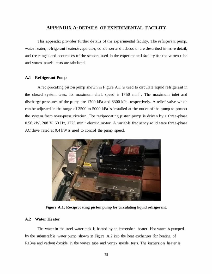
75
APPENDIX A: DETAILS OF EXPERIMENTAL FACILITY
This appendix provides further details of the experimental facility. The refrigerant pump,
water heater, refrigerant heater/evaporator, condenser and subcooler are described in more detail,
and the ranges and accuracies of the sensors used in the experimental facility for the vortex tube
and vortex nozzle tests are tabulated.
A.1 Refrigerant Pump
A reciprocating piston pump shown in Figure A.1 is used to circulate liquid refrigerant in
the closed system tests. Its maximum shaft speed is 1750 min-1. The maximum inlet and
discharge pressures of the pump are 1700 kPa and 8300 kPa, respectively. A relief valve which
can be adjusted in the range of 2500 to 5000 kPa is installed at the outlet of the pump to protect
the system from over-pressurization. The reciprocating piston pump is driven by a three-phase
0.56 kW, 208 V, 60 Hz, 1725 min-1 electric motor. A variable frequency solid state three-phase
AC drive rated at 0.4 kW is used to control the pump speed.
Figure A.1: Reciprocating piston pump for circulating liquid refrigerant.
A.2 Water Heater
The water in the steel water tank is heated by an immersion heater. Hot water is pumped
by the submersible water pump shown in Figure A.2 into the heat exchanger for heating of
R134a and carbon dioxide in the vortex tube and vortex nozzle tests. The immersion heater is
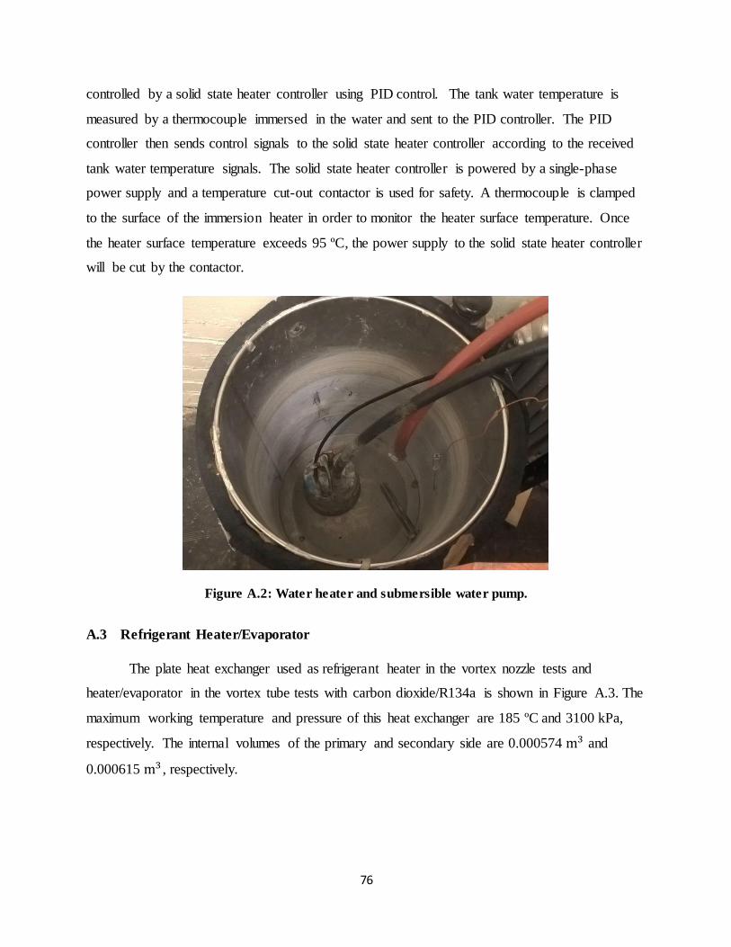
76
controlled by a solid state heater controller using PID control. The tank water temperature is
measured by a thermocouple immersed in the water and sent to the PID controller. The PID
controller then sends control signals to the solid state heater controller according to the received
tank water temperature signals. The solid state heater controller is powered by a single-phase
power supply and a temperature cut-out contactor is used for safety. A thermocouple is clamped
to the surface of the immersion heater in order to monitor the heater surface temperature. Once
the heater surface temperature exceeds 95 ºC, the power supply to the solid state heater controller
will be cut by the contactor.
Figure A.2: Water heater and submersible water pump.
A.3 Refrigerant Heater/Evaporator
The plate heat exchanger used as refrigerant heater in the vortex nozzle tests and
heater/evaporator in the vortex tube tests with carbon dioxide/R134a is shown in Figure A.3. The
maximum working temperature and pressure of this heat exchanger are 185 ºC and 3100 kPa,
respectively. The internal volumes of the primary and secondary side are 0.000574 m3 and
0.000615 m3 , respectively.

77
Figure A.3: Plate heat exchanger used as heater/evaporator in vortex nozzle and vortex tube tests.
A.4 Condenser and Subcooler
Two identical plate heat exchangers, as is shown in Figure A.4, are used as condenser and
subcooler, respectively, in the experimental facility for closed system tests. An accumulator is
installed between the condenser and the subcooler so that only liquid is allowed to enter the
subcooler. The subcooler is used to provide subcooling and guarantees that there is no cavitation
at the refrigerant pump inlet. The design maximum pressure of the heat exchangers is 3000 kPa
for both fluid sides. The allowed temperature range for these two heat exchangers is -160 ºC to
225 ºC.
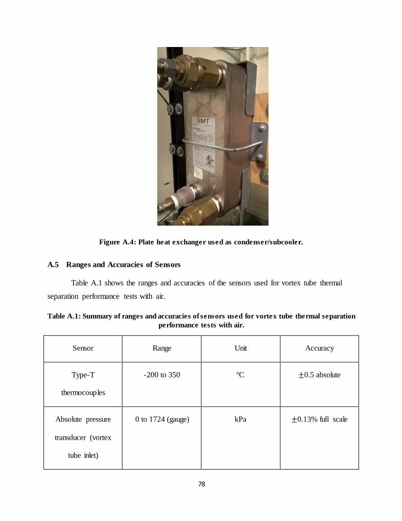
78
Figure A.4: Plate heat exchanger used as condenser/subcooler.
A.5 Ranges and Accuracies of Sensors
Table A.1 shows the ranges and accuracies of the sensors used for vortex tube thermal
separation performance tests with air.
Table A.1: Summary of ranges and accuracies of sensors used for vortex tube thermal separation
performance tests with air.
Sensor Range Unit Accuracy
Type-T
thermocouples
-200 to 350 ºC ±0.5 absolute
Absolute pressure
transducer (vortex
tube inlet)
0 to 1724 (gauge) kPa ±0.13% full scale
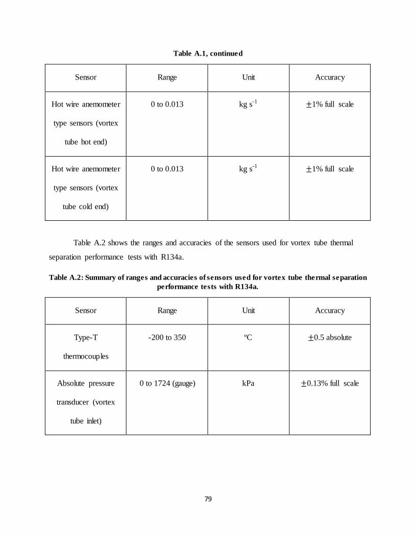
79
Table A.1, continued
Sensor Range Unit Accuracy
Hot wire anemometer
type sensors (vortex
tube hot end)
0 to 0.013 kg s-1 ±1% full scale
Hot wire anemometer
type sensors (vortex
tube cold end)
0 to 0.013 kg s-1 ±1% full scale
Table A.2 shows the ranges and accuracies of the sensors used for vortex tube thermal
separation performance tests with R134a.
Table A.2: Summary of ranges and accuracies of sensors used for vortex tube thermal separation
performance tests with R134a.
Sensor Range Unit Accuracy
Type-T
thermocouples
-200 to 350 ºC ±0.5 absolute
Absolute pressure
transducer (vortex
tube inlet)
0 to 1724 (gauge) kPa ±0.13% full scale
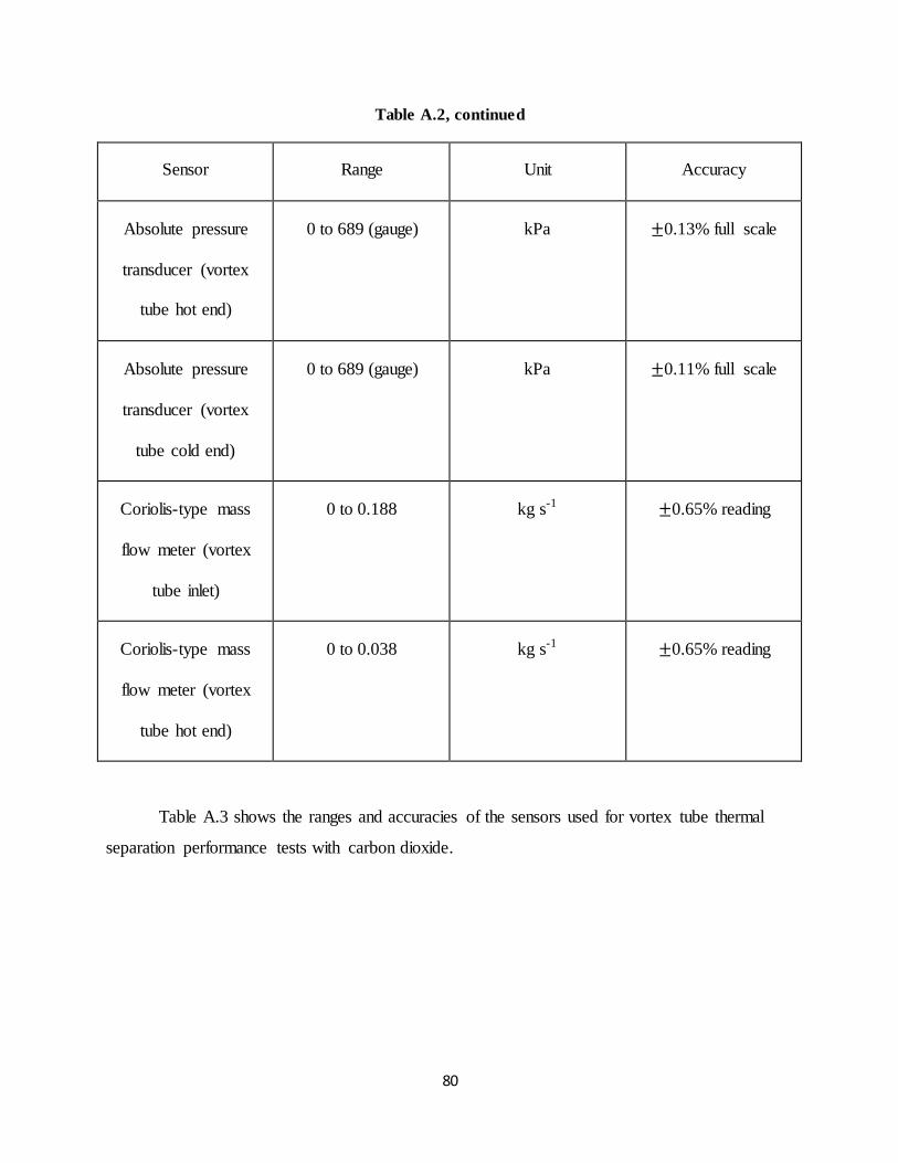
80
Table A.2, continued
Sensor Range Unit Accuracy
Absolute pressure
transducer (vortex
tube hot end)
0 to 689 (gauge) kPa ±0.13% full scale
Absolute pressure
transducer (vortex
tube cold end)
0 to 689 (gauge) kPa ±0.11% full scale
Coriolis-type mass
flow meter (vortex
tube inlet)
0 to 0.188 kg s-1 ±0.65% reading
Coriolis-type mass
flow meter (vortex
tube hot end)
0 to 0.038 kg s-1 ±0.65% reading
Table A.3 shows the ranges and accuracies of the sensors used for vortex tube thermal
separation performance tests with carbon dioxide.
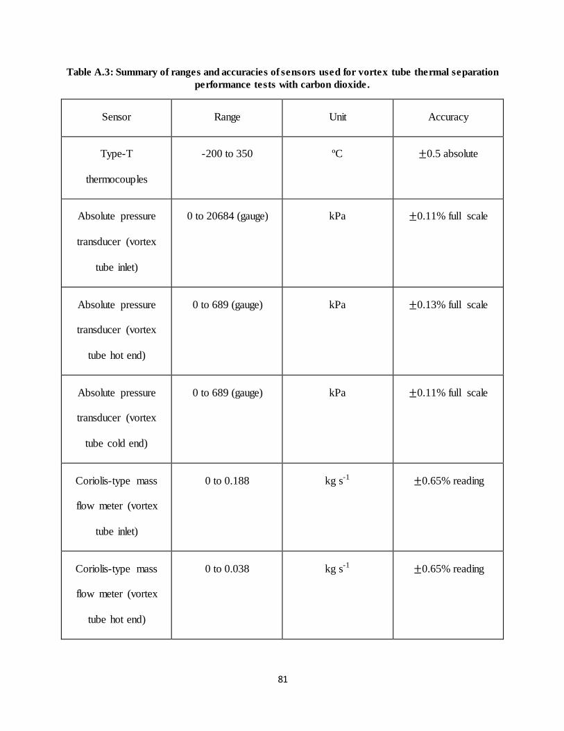
81
Table A.3: Summary of ranges and accuracies of sensors used for vortex tube thermal separation
performance tests with carbon dioxide.
Sensor Range Unit Accuracy
Type-T
thermocouples
-200 to 350 ºC ±0.5 absolute
Absolute pressure
transducer (vortex
tube inlet)
0 to 20684 (gauge) kPa ±0.11% full scale
Absolute pressure
transducer (vortex
tube hot end)
0 to 689 (gauge) kPa ±0.13% full scale
Absolute pressure
transducer (vortex
tube cold end)
0 to 689 (gauge) kPa ±0.11% full scale
Coriolis-type mass
flow meter (vortex
tube inlet)
0 to 0.188 kg s-1 ±0.65% reading
Coriolis-type mass
flow meter (vortex
tube hot end)
0 to 0.038 kg s-1 ±0.65% reading
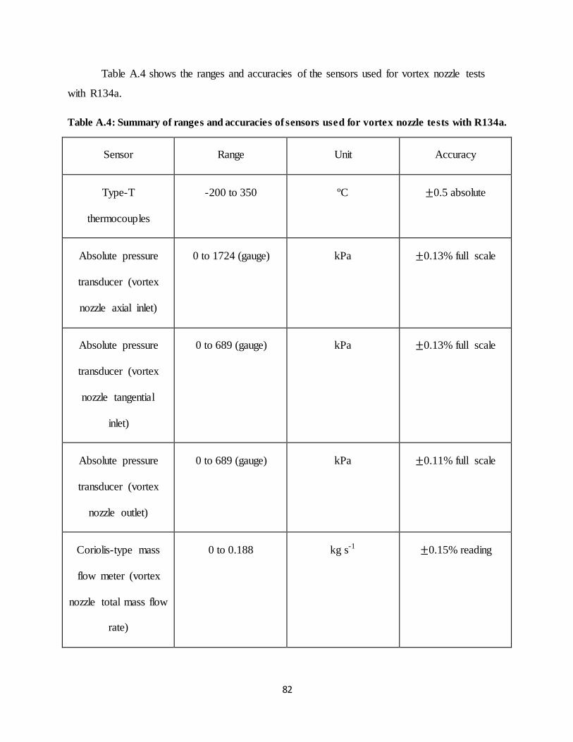
82
Table A.4 shows the ranges and accuracies of the sensors used for vortex nozzle tests
with R134a.
Table A.4: Summary of ranges and accuracies of sensors used for vortex nozzle tests with R134a.
Sensor Range Unit Accuracy
Type-T
thermocouples
-200 to 350 ºC ±0.5 absolute
Absolute pressure
transducer (vortex
nozzle axial inlet)
0 to 1724 (gauge) kPa ±0.13% full scale
Absolute pressure
transducer (vortex
nozzle tangential
inlet)
0 to 689 (gauge) kPa ±0.13% full scale
Absolute pressure
transducer (vortex
nozzle outlet)
0 to 689 (gauge) kPa ±0.11% full scale
Coriolis-type mass
flow meter (vortex
nozzle total mass flow
rate)
0 to 0.188 kg s-1 ±0.15% reading
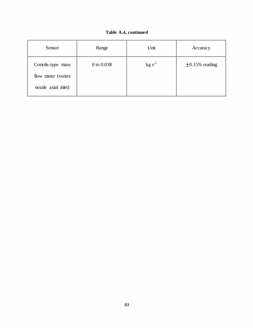
83
Table A.4, continued
Sensor Range Unit Accuracy
Coriolis-type mass
flow meter (vortex
nozzle axial inlet)
0 to 0.038 kg s-1 ±0.15% reading
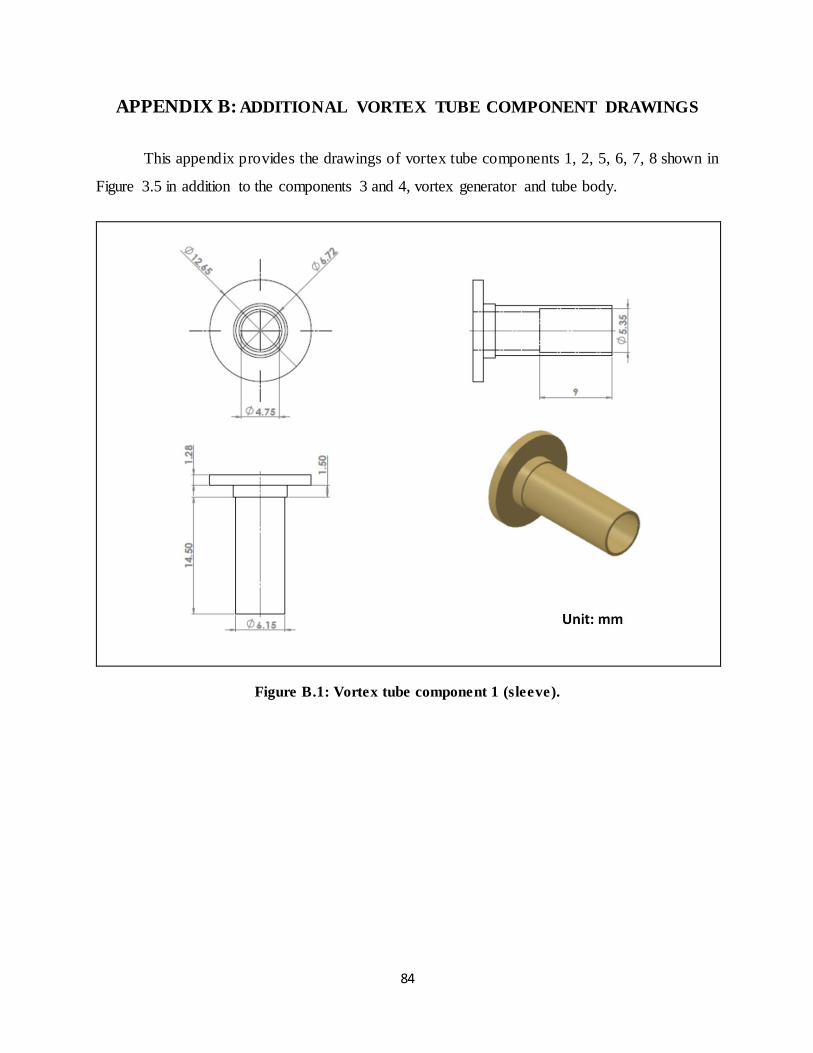
84
APPENDIX B: ADDITIONAL VORTEX TUBE COMPONENT DRAWINGS
This appendix provides the drawings of vortex tube components 1, 2, 5, 6, 7, 8 shown in
Figure 3.5 in addition to the components 3 and 4, vortex generator and tube body.
Figure B.1: Vortex tube component 1 (sleeve).
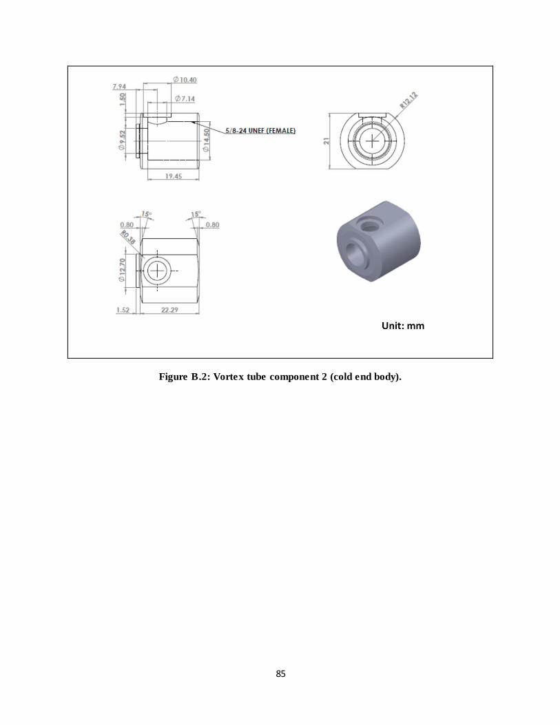
85
Figure B.2: Vortex tube component 2 (cold end body).
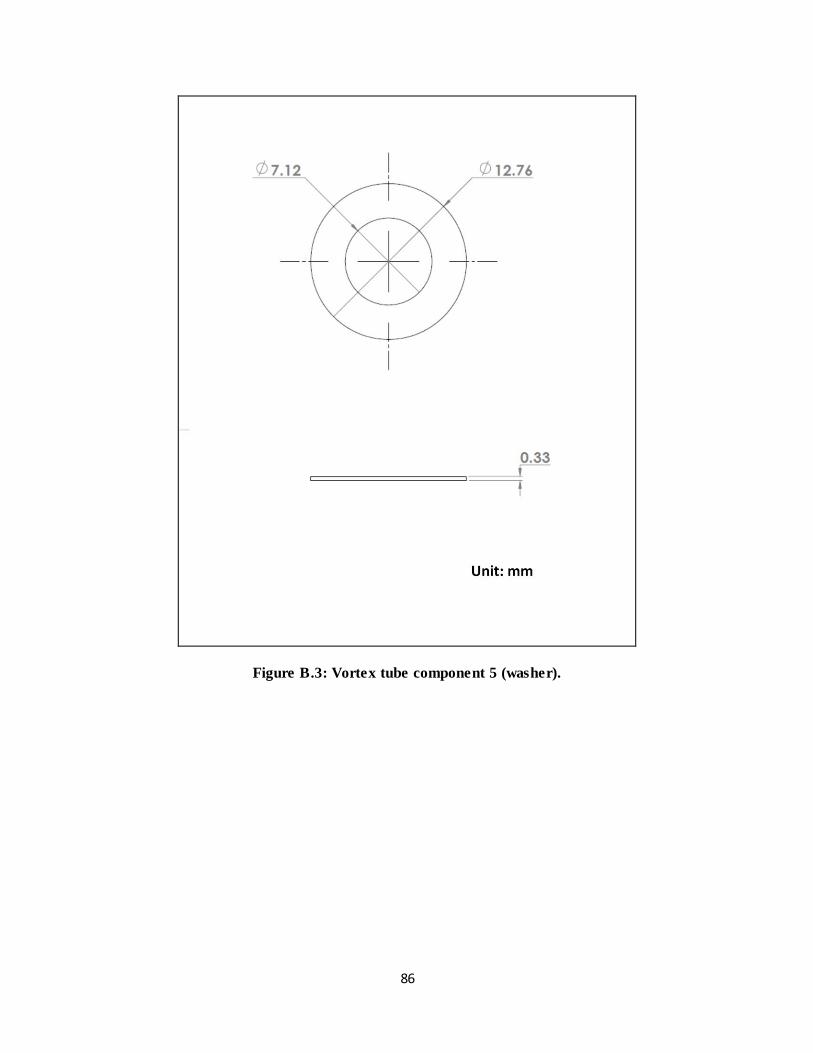
86
Figure B.3: Vortex tube component 5 (washer).
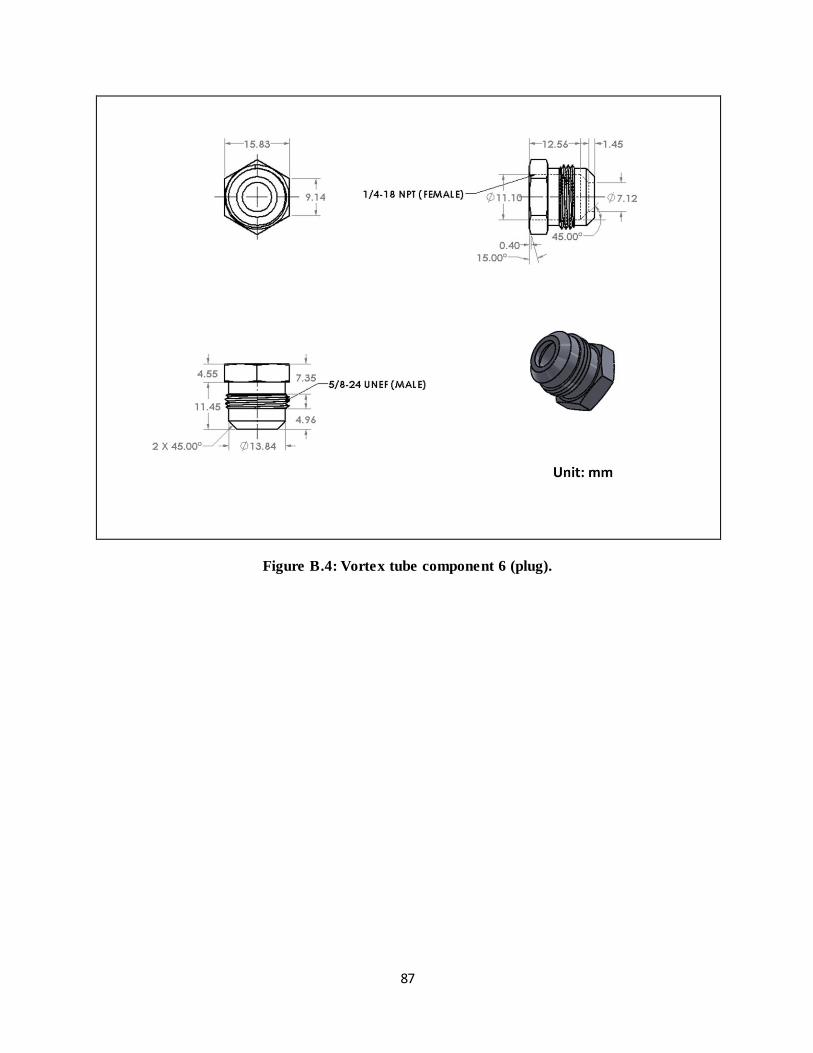
87
Figure B.4: Vortex tube component 6 (plug).
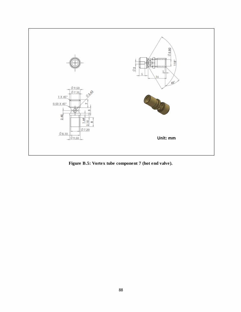
88
Figure B.5: Vortex tube component 7 (hot end valve).
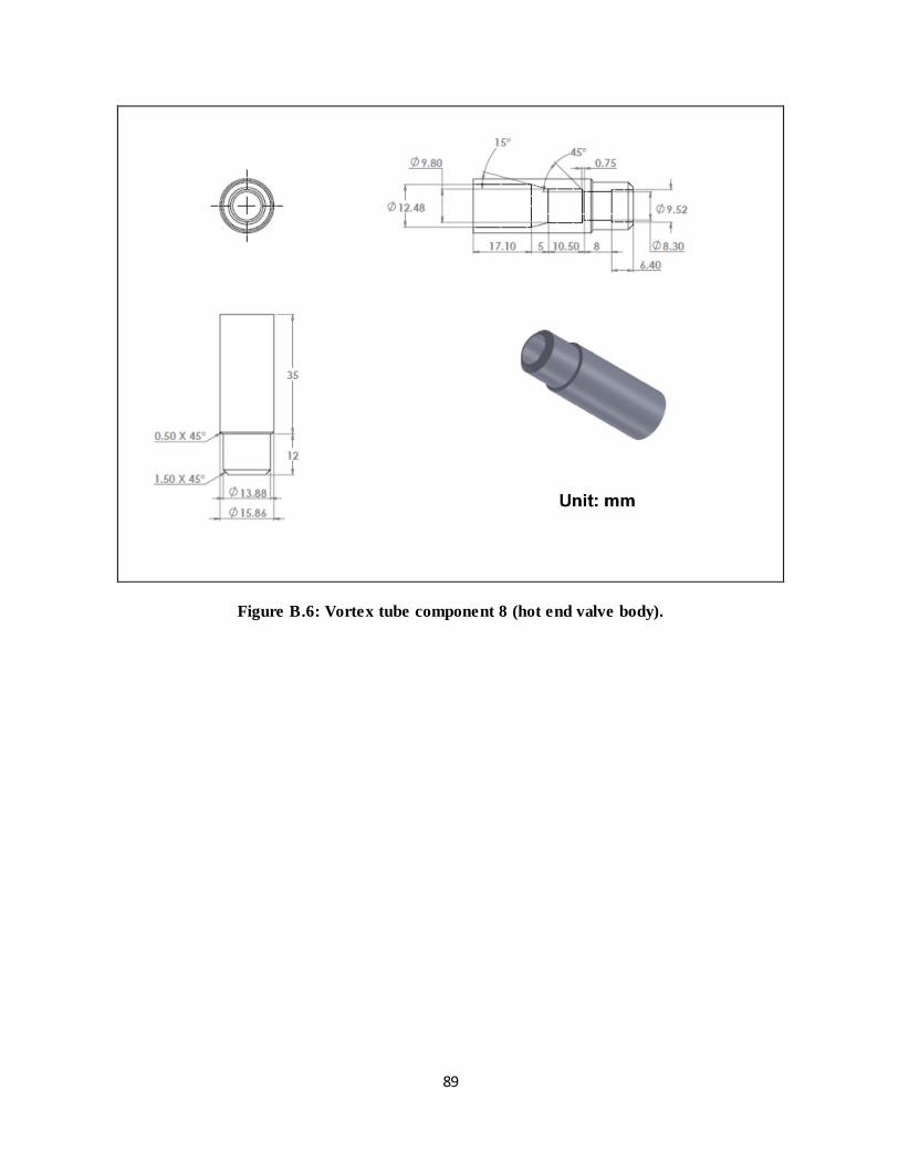
89
Figure B.6: Vortex tube component 8 (hot end valve body).
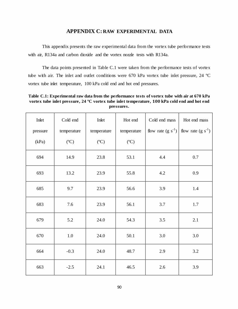
90
APPENDIX C: RAW EXPERIMENTAL DATA
This appendix presents the raw experimental data from the vortex tube performance tests
with air, R134a and carbon dioxide and the vortex nozzle tests with R134a.
The data points presented in Table C.1 were taken from the performance tests of vortex
tube with air. The inlet and outlet conditions were 670 kPa vortex tube inlet pressure, 24 ºC
vortex tube inlet temperature, 100 kPa cold end and hot end pressures.
Table C.1: Experimental raw data from the performance tests of vortex tube with air at 670 kPa
vortex tube inlet pressure, 24 ºC vortex tube inlet temperature, 𝟏𝟎𝟎 𝐤𝐏𝐚 cold end and hot end
pressures.
Inlet
pressure
(kPa)
Cold end
temperature
(ºC)
Inlet
temperature
(ºC)
Hot end
temperature
(ºC)
Cold end mass
flow rate (g s-1)
Hot end mass
flow rate (g s-1)
694 14.9 23.8 53.1 4.4 0.7
693 13.2 23.9 55.8 4.2 0.9
685 9.7 23.9 56.6 3.9 1.4
683 7.6 23.9 56.1 3.7 1.7
679 5.2 24.0 54.3 3.5 2.1
670 1.0 24.0 50.1 3.0 3.0
664 -0.3 24.0 48.7 2.9 3.2
663 -2.5 24.1 46.5 2.6 3.9
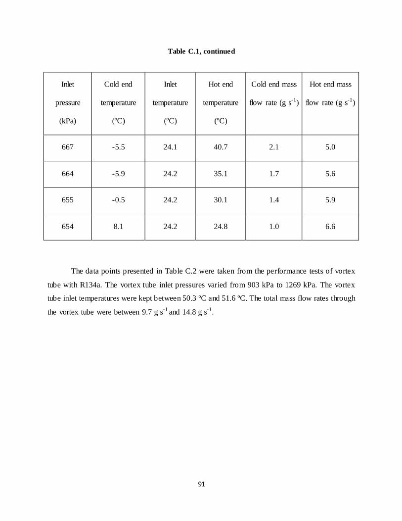
91
Table C.1, continued
Inlet
pressure
(kPa)
Cold end
temperature
(ºC)
Inlet
temperature
(ºC)
Hot end
temperature
(ºC)
Cold end mass
flow rate (g s-1)
Hot end mass
flow rate (g s-1)
667 -5.5 24.1 40.7 2.1 5.0
664 -5.9 24.2 35.1 1.7 5.6
655 -0.5 24.2 30.1 1.4 5.9
654 8.1 24.2 24.8 1.0 6.6
The data points presented in Table C.2 were taken from the performance tests of vortex
tube with R134a. The vortex tube inlet pressures varied from 903 kPa to 1269 kPa. The vortex
tube inlet temperatures were kept between 50.3 ºC and 51.6 ºC. The total mass flow rates through
the vortex tube were between 9.7 g s-1 and 14.8 g s-1.
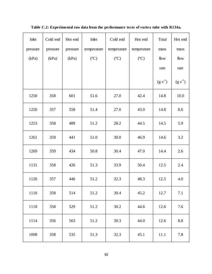
92
Table C.2: Experimental raw data from the performance tests of vortex tube with R134a.
Inlet
pressure
(kPa)
Cold end
pressure
(kPa)
Hot end
pressure
(kPa)
Inlet
temperature
(ºC)
Cold end
temperature
(ºC)
Hot end
temperature
(ºC)
Total
mass
flow
rate
(g s-1)
Hot end
mass
flow
rate
(g s-1)
1250 358 601 51.6 27.0 42.4 14.8 10.0
1250 357 558 51.4 27.0 43.0 14.8 8.6
1253 358 489 51.2 28.2 44.5 14.5 5.9
1261 359 441 51.0 30.0 46.9 14.6 3.2
1269 359 434 50.8 30.4 47.0 14.4 2.6
1131 358 426 51.3 33.9 50.4 12.5 2.4
1126 357 446 51.2 32.3 48.3 12.5 4.0
1116 358 514 51.2 30.4 45.2 12.7 7.1
1118 358 529 51.2 30.2 44.6 12.6 7.6
1114 356 563 51.2 30.3 44.0 12.6 8.8
1008 358 535 51.3 32.3 45.1 11.1 7.8
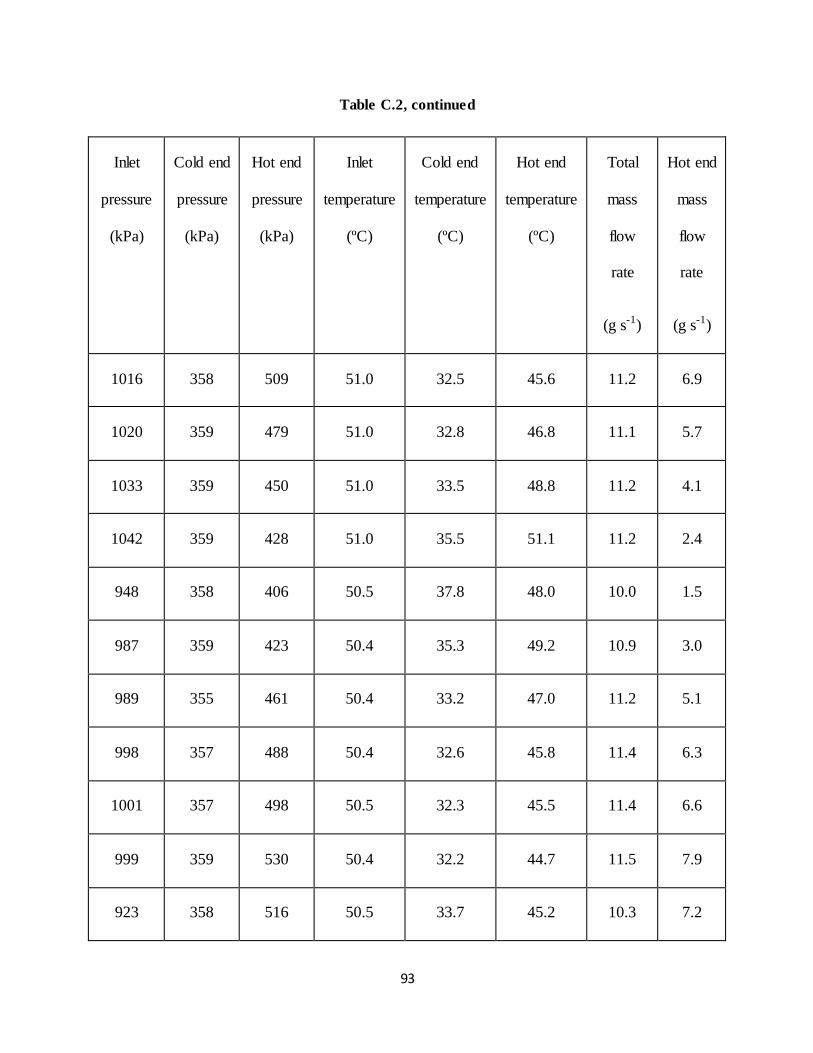
93
Table C.2, continued
Inlet
pressure
(kPa)
Cold end
pressure
(kPa)
Hot end
pressure
(kPa)
Inlet
temperature
(ºC)
Cold end
temperature
(ºC)
Hot end
temperature
(ºC)
Total
mass
flow
rate
(g s-1)
Hot end
mass
flow
rate
(g s-1)
1016 358 509 51.0 32.5 45.6 11.2 6.9
1020 359 479 51.0 32.8 46.8 11.1 5.7
1033 359 450 51.0 33.5 48.8 11.2 4.1
1042 359 428 51.0 35.5 51.1 11.2 2.4
948 358 406 50.5 37.8 48.0 10.0 1.5
987 359 423 50.4 35.3 49.2 10.9 3.0
989 355 461 50.4 33.2 47.0 11.2 5.1
998 357 488 50.4 32.6 45.8 11.4 6.3
1001 357 498 50.5 32.3 45.5 11.4 6.6
999 359 530 50.4 32.2 44.7 11.5 7.9
923 358 516 50.5 33.7 45.2 10.3 7.2
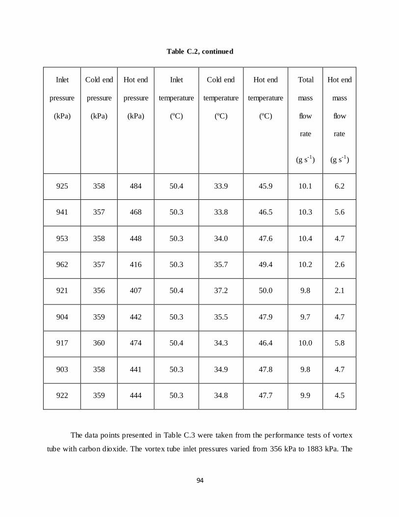
94
Table C.2, continued
Inlet
pressure
(kPa)
Cold end
pressure
(kPa)
Hot end
pressure
(kPa)
Inlet
temperature
(ºC)
Cold end
temperature
(ºC)
Hot end
temperature
(ºC)
Total
mass
flow
rate
(g s-1)
Hot end
mass
flow
rate
(g s-1)
925 358 484 50.4 33.9 45.9 10.1 6.2
941 357 468 50.3 33.8 46.5 10.3 5.6
953 358 448 50.3 34.0 47.6 10.4 4.7
962 357 416 50.3 35.7 49.4 10.2 2.6
921 356 407 50.4 37.2 50.0 9.8 2.1
904 359 442 50.3 35.5 47.9 9.7 4.7
917 360 474 50.4 34.3 46.4 10.0 5.8
903 358 441 50.3 34.9 47.8 9.8 4.7
922 359 444 50.3 34.8 47.7 9.9 4.5
The data points presented in Table C.3 were taken from the performance tests of vortex
tube with carbon dioxide. The vortex tube inlet pressures varied from 356 kPa to 1883 kPa. The
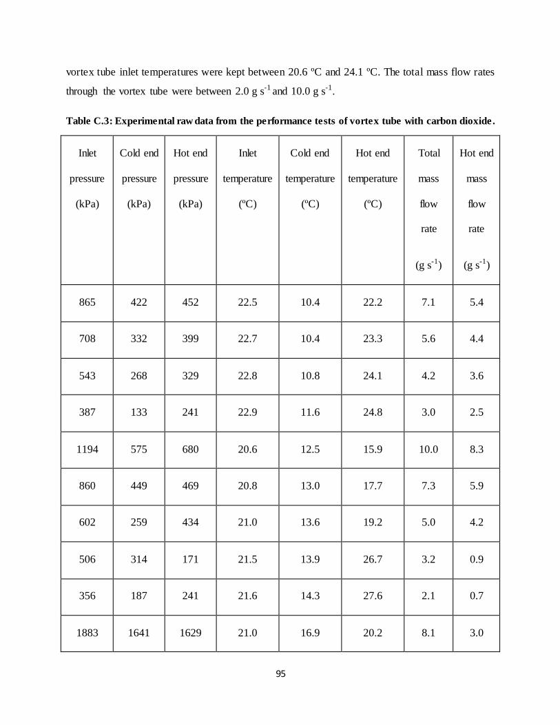
95
vortex tube inlet temperatures were kept between 20.6 ºC and 24.1 ºC. The total mass flow rates
through the vortex tube were between 2.0 g s-1 and 10.0 g s-1.
Table C.3: Experimental raw data from the performance tests of vortex tube with carbon dioxide.
Inlet
pressure
(kPa)
Cold end
pressure
(kPa)
Hot end
pressure
(kPa)
Inlet
temperature
(ºC)
Cold end
temperature
(ºC)
Hot end
temperature
(ºC)
Total
mass
flow
rate
(g s-1)
Hot end
mass
flow
rate
(g s-1)
865 422 452 22.5 10.4 22.2 7.1 5.4
708 332 399 22.7 10.4 23.3 5.6 4.4
543 268 329 22.8 10.8 24.1 4.2 3.6
387 133 241 22.9 11.6 24.8 3.0 2.5
1194 575 680 20.6 12.5 15.9 10.0 8.3
860 449 469 20.8 13.0 17.7 7.3 5.9
602 259 434 21.0 13.6 19.2 5.0 4.2
506 314 171 21.5 13.9 26.7 3.2 0.9
356 187 241 21.6 14.3 27.6 2.1 0.7
1883 1641 1629 21.0 16.9 20.2 8.1 3.0
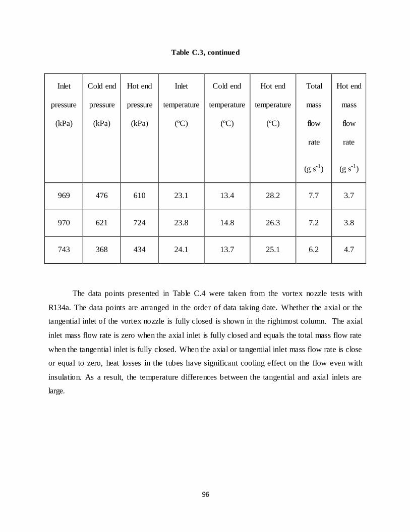
96
Table C.3, continued
Inlet
pressure
(kPa)
Cold end
pressure
(kPa)
Hot end
pressure
(kPa)
Inlet
temperature
(ºC)
Cold end
temperature
(ºC)
Hot end
temperature
(ºC)
Total
mass
flow
rate
(g s-1)
Hot end
mass
flow
rate
(g s-1)
969 476 610 23.1 13.4 28.2 7.7 3.7
970 621 724 23.8 14.8 26.3 7.2 3.8
743 368 434 24.1 13.7 25.1 6.2 4.7
The data points presented in Table C.4 were taken from the vortex nozzle tests with
R134a. The data points are arranged in the order of data taking date. Whether the axial or the
tangential inlet of the vortex nozzle is fully closed is shown in the rightmost column. The axial
inlet mass flow rate is zero when the axial inlet is fully closed and equals the total mass flow rate
when the tangential inlet is fully closed. When the axial or tangential inlet mass flow rate is close
or equal to zero, heat losses in the tubes have significant cooling effect on the flow even with
insulation. As a result, the temperature differences between the tangential and axial inlets are
large.
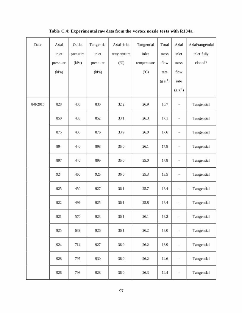
97
Table C.4: Experimental raw data from the vortex nozzle tests with R134a.
Date Axial
inlet
pressure
(kPa)
Outlet
pressure
(kPa)
Tangential
inlet
pressure
(kPa)
Axial inlet
temperature
(ºC)
Tangential
inlet
temperature
(ºC)
Total
mass
flow
rate
(g s-1
)
Axial
inlet
mass
flow
rate
(g s-1
)
Axial/tangential
inlet fully
closed?
8/8/2015 828 430 830 32.2 26.9 16.7 - Tangential
850 433 852 33.1 26.3 17.1 - Tangential
875 436 876 33.9 26.0 17.6 - Tangential
894 440 898 35.0 26.1 17.8 - Tangential
897 440 899 35.0 25.0 17.8 - Tangential
924 450 925 36.0 25.3 18.5 - Tangential
925 450 927 36.1 25.7 18.4 - Tangential
922 499 925 36.1 25.8 18.4 - Tangential
921 570 923 36.1 26.1 18.2 - Tangential
925 639 926 36.1 26.2 18.0 - Tangential
924 714 927 36.0 26.2 16.9 - Tangential
928 797 930 36.0 26.2 14.6 - Tangential
926 796 928 36.0 26.3 14.4 - Tangential
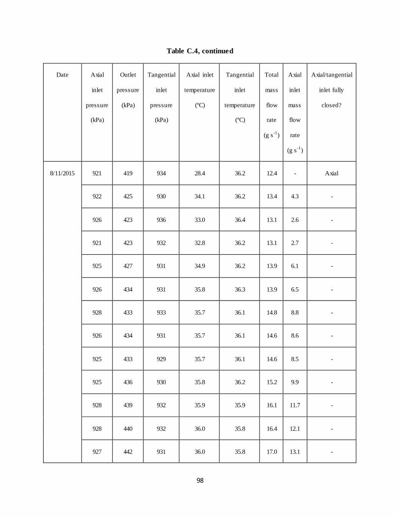
98
Table C.4, continued
Date Axial
inlet
pressure
(kPa)
Outlet
pressure
(kPa)
Tangential
inlet
pressure
(kPa)
Axial inlet
temperature
(ºC)
Tangential
inlet
temperature
(ºC)
Total
mass
flow
rate
(g s-1
)
Axial
inlet
mass
flow
rate
(g s-1
)
Axial/tangential
inlet fully
closed?
8/11/2015 921 419 934 28.4 36.2 12.4 - Axial
922 425 930 34.1 36.2 13.4 4.3 -
926 423 936 33.0 36.4 13.1 2.6 -
921 423 932 32.8 36.2 13.1 2.7 -
925 427 931 34.9 36.2 13.9 6.1 -
926 434 931 35.8 36.3 13.9 6.5 -
928 433 933 35.7 36.1 14.8 8.8 -
926 434 931 35.7 36.1 14.6 8.6 -
925 433 929 35.7 36.1 14.6 8.5 -
925 436 930 35.8 36.2 15.2 9.9 -
928 439 932 35.9 35.9 16.1 11.7 -
928 440 932 36.0 35.8 16.4 12.1 -
927 442 931 36.0 35.8 17.0 13.1 -
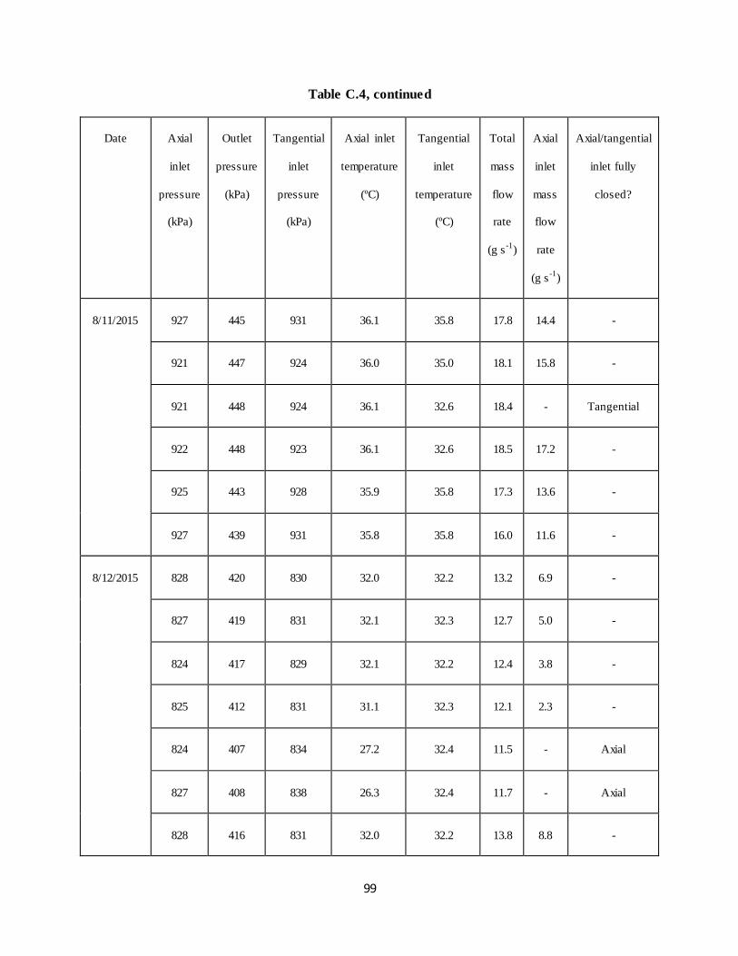
99
Table C.4, continued
Date Axial
inlet
pressure
(kPa)
Outlet
pressure
(kPa)
Tangential
inlet
pressure
(kPa)
Axial inlet
temperature
(ºC)
Tangential
inlet
temperature
(ºC)
Total
mass
flow
rate
(g s-1
)
Axial
inlet
mass
flow
rate
(g s-1
)
Axial/tangential
inlet fully
closed?
8/11/2015 927 445 931 36.1 35.8 17.8 14.4 -
921 447 924 36.0 35.0 18.1 15.8 -
921 448 924 36.1 32.6 18.4 - Tangential
922 448 923 36.1 32.6 18.5 17.2 -
925 443 928 35.9 35.8 17.3 13.6 -
927 439 931 35.8 35.8 16.0 11.6 -
8/12/2015 828 420 830 32.0 32.2 13.2 6.9 -
827 419 831 32.1 32.3 12.7 5.0 -
824 417 829 32.1 32.2 12.4 3.8 -
825 412 831 31.1 32.3 12.1 2.3 -
824 407 834 27.2 32.4 11.5 - Axial
827 408 838 26.3 32.4 11.7 - Axial
828 416 831 32.0 32.2 13.8 8.8 -
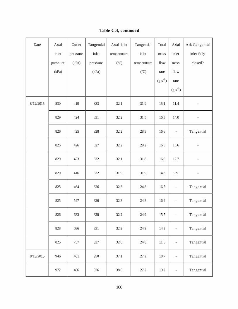
100
Table C.4, continued
Date Axial
inlet
pressure
(kPa)
Outlet
pressure
(kPa)
Tangential
inlet
pressure
(kPa)
Axial inlet
temperature
(ºC)
Tangential
inlet
temperature
(ºC)
Total
mass
flow
rate
(g s-1
)
Axial
inlet
mass
flow
rate
(g s-1
)
Axial/tangential
inlet fully
closed?
8/12/2015 830 419 833 32.1 31.9 15.1 11.4 -
829 424 831 32.2 31.5 16.3 14.0 -
826 425 828 32.2 28.9 16.6 - Tangential
825 426 827 32.2 29.2 16.5 15.6 -
829 423 832 32.1 31.8 16.0 12.7 -
829 416 832 31.9 31.9 14.3 9.9 -
825 464 826 32.3 24.8 16.5 - Tangential
825 547 826 32.3 24.8 16.4 - Tangential
826 633 828 32.2 24.9 15.7 - Tangential
828 686 831 32.2 24.9 14.3 - Tangential
825 757 827 32.0 24.8 11.5 - Tangential
8/13/2015 946 461 950 37.1 27.2 18.7 - Tangential
972 466 976 38.0 27.2 19.2 - Tangential
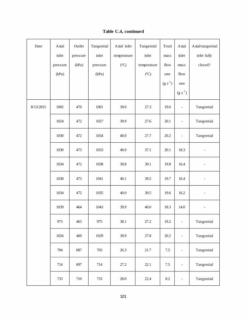
101
Table C.4, continued
Date Axial
inlet
pressure
(kPa)
Outlet
pressure
(kPa)
Tangential
inlet
pressure
(kPa)
Axial inlet
temperature
(ºC)
Tangential
inlet
temperature
(ºC)
Total
mass
flow
rate
(g s-1
)
Axial
inlet
mass
flow
rate
(g s-1
)
Axial/tangential
inlet fully
closed?
8/13/2015 1002 470 1001 39.0 27.3 19.6 - Tangential
1024 472 1027 39.9 27.6 20.1 - Tangential
1030 472 1034 40.0 27.7 20.2 - Tangential
1030 473 1033 40.0 37.1 20.1 18.3 -
1034 472 1038 39.8 39.1 19.8 16.4 -
1038 473 1041 40.1 39.5 19.7 16.4 -
1034 472 1035 40.0 39.5 19.6 16.2 -
1039 464 1043 39.9 40.0 18.3 14.0 -
973 463 975 38.1 27.2 19.2 - Tangential
1026 469 1029 39.9 27.8 20.2 - Tangential
704 687 703 26.3 21.7 7.5 - Tangential
714 697 714 27.2 22.1 7.5 - Tangential
733 710 733 28.0 22.4 8.2 - Tangential
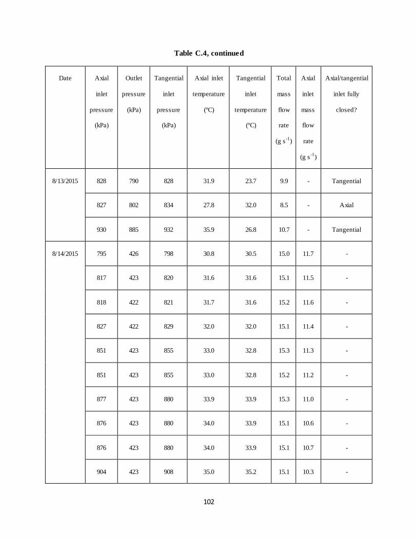
102
Table C.4, continued
Date Axial
inlet
pressure
(kPa)
Outlet
pressure
(kPa)
Tangential
inlet
pressure
(kPa)
Axial inlet
temperature
(ºC)
Tangential
inlet
temperature
(ºC)
Total
mass
flow
rate
(g s-1
)
Axial
inlet
mass
flow
rate
(g s-1
)
Axial/tangential
inlet fully
closed?
8/13/2015 828 790 828 31.9 23.7 9.9 - Tangential
827 802 834 27.8 32.0 8.5 - Axial
930 885 932 35.9 26.8 10.7 - Tangential
8/14/2015 795 426 798 30.8 30.5 15.0 11.7 -
817 423 820 31.6 31.6 15.1 11.5 -
818 422 821 31.7 31.6 15.2 11.6 -
827 422 829 32.0 32.0 15.1 11.4 -
851 423 855 33.0 32.8 15.3 11.3 -
851 423 855 33.0 32.8 15.2 11.2 -
877 423 880 33.9 33.9 15.3 11.0 -
876 423 880 34.0 33.9 15.1 10.6 -
876 423 880 34.0 33.9 15.1 10.7 -
904 423 908 35.0 35.2 15.1 10.3 -
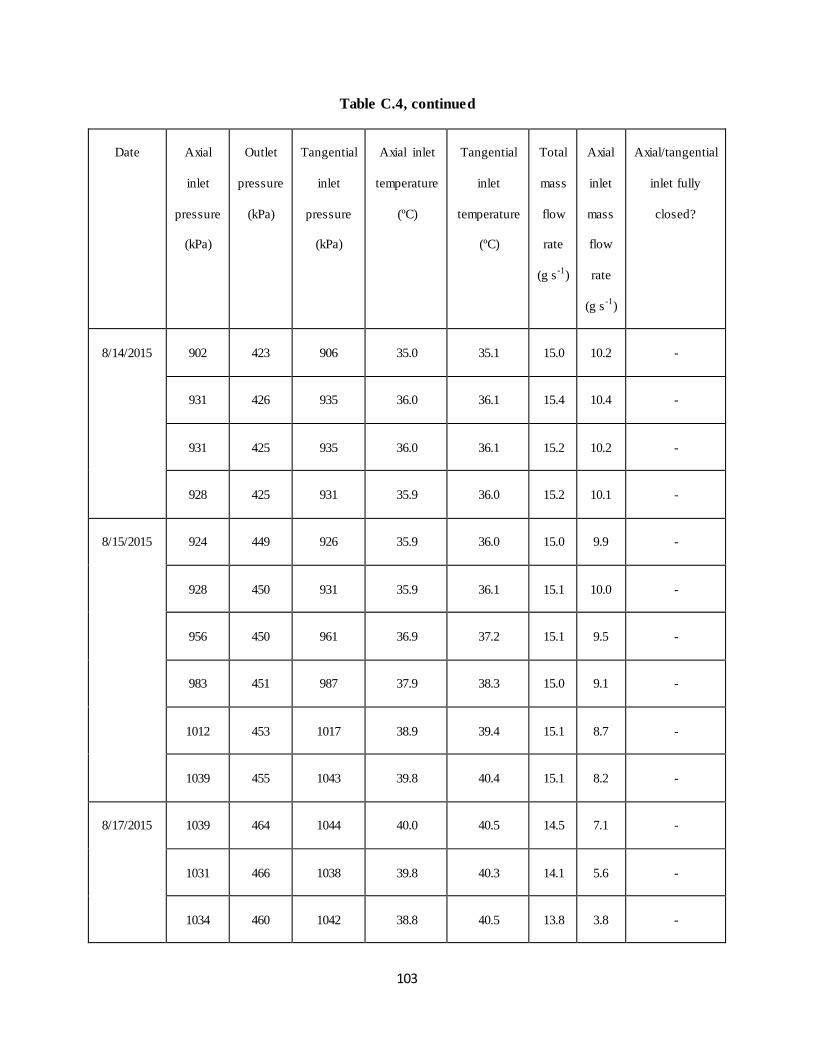
103
Table C.4, continued
Date Axial
inlet
pressure
(kPa)
Outlet
pressure
(kPa)
Tangential
inlet
pressure
(kPa)
Axial inlet
temperature
(ºC)
Tangential
inlet
temperature
(ºC)
Total
mass
flow
rate
(g s-1
)
Axial
inlet
mass
flow
rate
(g s-1
)
Axial/tangential
inlet fully
closed?
8/14/2015 902 423 906 35.0 35.1 15.0 10.2 -
931 426 935 36.0 36.1 15.4 10.4 -
931 425 935 36.0 36.1 15.2 10.2 -
928 425 931 35.9 36.0 15.2 10.1 -
8/15/2015 924 449 926 35.9 36.0 15.0 9.9 -
928 450 931 35.9 36.1 15.1 10.0 -
956 450 961 36.9 37.2 15.1 9.5 -
983 451 987 37.9 38.3 15.0 9.1 -
1012 453 1017 38.9 39.4 15.1 8.7 -
1039 455 1043 39.8 40.4 15.1 8.2 -
8/17/2015 1039 464 1044 40.0 40.5 14.5 7.1 -
1031 466 1038 39.8 40.3 14.1 5.6 -
1034 460 1042 38.8 40.5 13.8 3.8 -
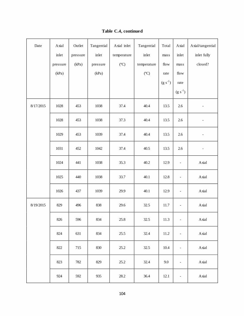
104
Table C.4, continued
Date Axial
inlet
pressure
(kPa)
Outlet
pressure
(kPa)
Tangential
inlet
pressure
(kPa)
Axial inlet
temperature
(ºC)
Tangential
inlet
temperature
(ºC)
Total
mass
flow
rate
(g s-1
)
Axial
inlet
mass
flow
rate
(g s-1
)
Axial/tangential
inlet fully
closed?
8/17/2015 1028 453 1038 37.4 40.4 13.5 2.6 -
1028 453 1038 37.3 40.4 13.5 2.6 -
1029 453 1039 37.4 40.4 13.5 2.6 -
1031 452 1042 37.4 40.5 13.5 2.6 -
1024 441 1038 35.3 40.2 12.9 - Axial
1025 440 1038 33.7 40.1 12.8 - Axial
1026 437 1039 29.9 40.1 12.9 - Axial
8/19/2015 829 496 838 29.6 32.5 11.7 - Axial
826 596 834 25.8 32.5 11.3 - Axial
824 631 834 25.5 32.4 11.2 - Axial
822 715 830 25.2 32.5 10.4 - Axial
823 782 829 25.2 32.4 9.0 - Axial
924 592 935 28.2 36.4 12.1 - Axial
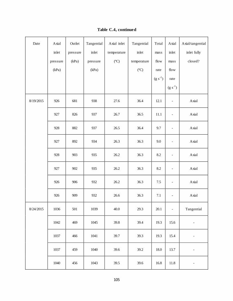
105
Table C.4, continued
Date Axial
inlet
pressure
(kPa)
Outlet
pressure
(kPa)
Tangential
inlet
pressure
(kPa)
Axial inlet
temperature
(ºC)
Tangential
inlet
temperature
(ºC)
Total
mass
flow
rate
(g s-1
)
Axial
inlet
mass
flow
rate
(g s-1
)
Axial/tangential
inlet fully
closed?
8/19/2015 926 681 938 27.6 36.4 12.1 - Axial
927 826 937 26.7 36.5 11.1 - Axial
928 882 937 26.5 36.4 9.7 - Axial
927 892 934 26.3 36.3 9.0 - Axial
928 903 935 26.2 36.3 8.2 - Axial
927 902 935 26.2 36.3 8.2 - Axial
926 906 932 26.2 36.3 7.5 - Axial
926 909 932 26.6 36.3 7.1 - Axial
8/24/2015 1036 501 1039 40.0 29.3 20.1 - Tangential
1042 469 1045 39.8 39.4 19.3 15.6 -
1037 466 1041 39.7 39.3 19.3 15.4 -
1037 459 1040 39.6 39.2 18.0 13.7 -
1040 456 1043 39.5 39.6 16.8 11.8 -
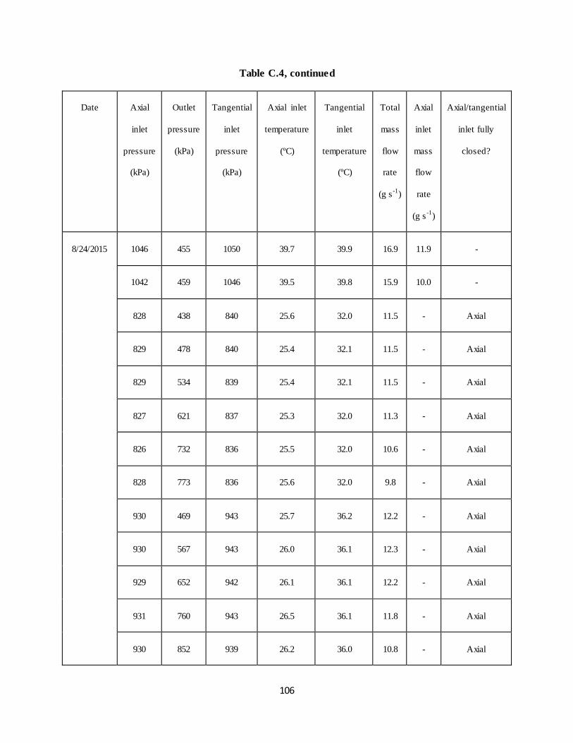
106
Table C.4, continued
Date Axial
inlet
pressure
(kPa)
Outlet
pressure
(kPa)
Tangential
inlet
pressure
(kPa)
Axial inlet
temperature
(ºC)
Tangential
inlet
temperature
(ºC)
Total
mass
flow
rate
(g s-1
)
Axial
inlet
mass
flow
rate
(g s-1
)
Axial/tangential
inlet fully
closed?
8/24/2015 1046 455 1050 39.7 39.9 16.9 11.9 -
1042 459 1046 39.5 39.8 15.9 10.0 -
828 438 840 25.6 32.0 11.5 - Axial
829 478 840 25.4 32.1 11.5 - Axial
829 534 839 25.4 32.1 11.5 - Axial
827 621 837 25.3 32.0 11.3 - Axial
826 732 836 25.5 32.0 10.6 - Axial
828 773 836 25.6 32.0 9.8 - Axial
930 469 943 25.7 36.2 12.2 - Axial
930 567 943 26.0 36.1 12.3 - Axial
929 652 942 26.1 36.1 12.2 - Axial
931 760 943 26.5 36.1 11.8 - Axial
930 852 939 26.2 36.0 10.8 - Axial
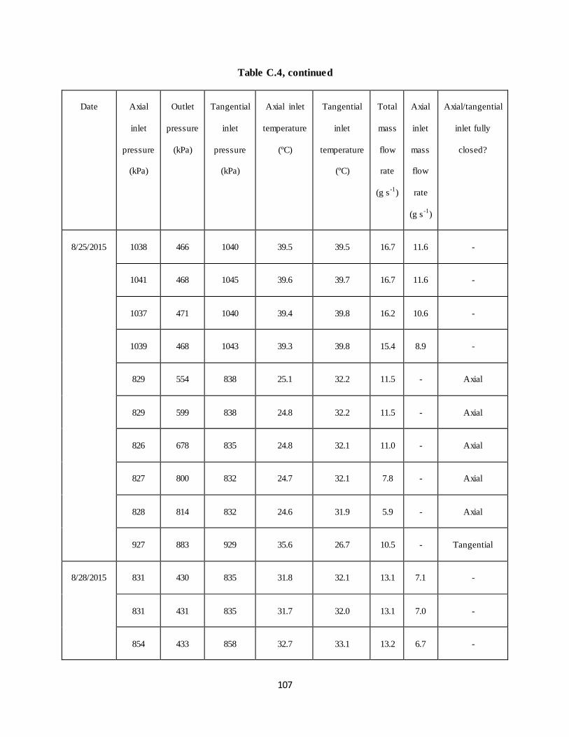
107
Table C.4, continued
Date Axial
inlet
pressure
(kPa)
Outlet
pressure
(kPa)
Tangential
inlet
pressure
(kPa)
Axial inlet
temperature
(ºC)
Tangential
inlet
temperature
(ºC)
Total
mass
flow
rate
(g s-1
)
Axial
inlet
mass
flow
rate
(g s-1
)
Axial/tangential
inlet fully
closed?
8/25/2015 1038 466 1040 39.5 39.5 16.7 11.6 -
1041 468 1045 39.6 39.7 16.7 11.6 -
1037 471 1040 39.4 39.8 16.2 10.6 -
1039 468 1043 39.3 39.8 15.4 8.9 -
829 554 838 25.1 32.2 11.5 - Axial
829 599 838 24.8 32.2 11.5 - Axial
826 678 835 24.8 32.1 11.0 - Axial
827 800 832 24.7 32.1 7.8 - Axial
828 814 832 24.6 31.9 5.9 - Axial
927 883 929 35.6 26.7 10.5 - Tangential
8/28/2015 831 430 835 31.8 32.1 13.1 7.1 -
831 431 835 31.7 32.0 13.1 7.0 -
854 433 858 32.7 33.1 13.2 6.7 -
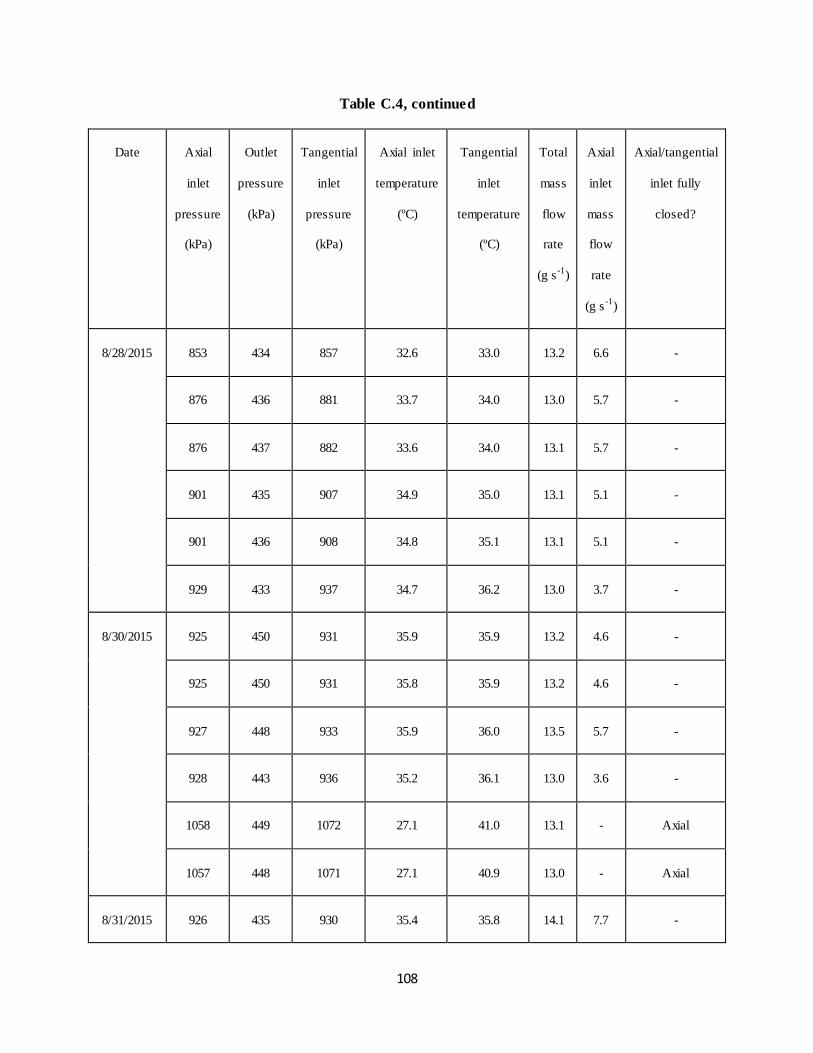
108
Table C.4, continued
Date Axial
inlet
pressure
(kPa)
Outlet
pressure
(kPa)
Tangential
inlet
pressure
(kPa)
Axial inlet
temperature
(ºC)
Tangential
inlet
temperature
(ºC)
Total
mass
flow
rate
(g s-1
)
Axial
inlet
mass
flow
rate
(g s-1
)
Axial/tangential
inlet fully
closed?
8/28/2015 853 434 857 32.6 33.0 13.2 6.6 -
876 436 881 33.7 34.0 13.0 5.7 -
876 437 882 33.6 34.0 13.1 5.7 -
901 435 907 34.9 35.0 13.1 5.1 -
901 436 908 34.8 35.1 13.1 5.1 -
929 433 937 34.7 36.2 13.0 3.7 -
8/30/2015 925 450 931 35.9 35.9 13.2 4.6 -
925 450 931 35.8 35.9 13.2 4.6 -
927 448 933 35.9 36.0 13.5 5.7 -
928 443 936 35.2 36.1 13.0 3.6 -
1058 449 1072 27.1 41.0 13.1 - Axial
1057 448 1071 27.1 40.9 13.0 - Axial
8/31/2015 926 435 930 35.4 35.8 14.1 7.7 -
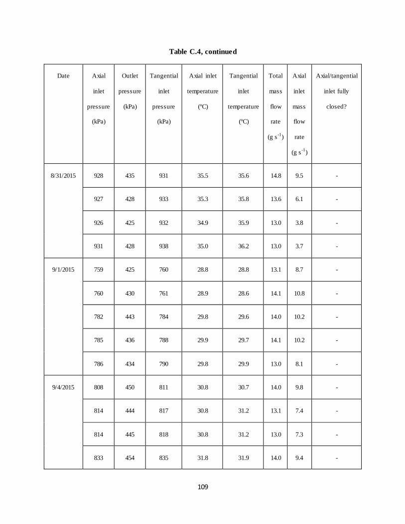
109
Table C.4, continued
Date Axial
inlet
pressure
(kPa)
Outlet
pressure
(kPa)
Tangential
inlet
pressure
(kPa)
Axial inlet
temperature
(ºC)
Tangential
inlet
temperature
(ºC)
Total
mass
flow
rate
(g s-1
)
Axial
inlet
mass
flow
rate
(g s-1
)
Axial/tangential
inlet fully
closed?
8/31/2015 928 435 931 35.5 35.6 14.8 9.5 -
927 428 933 35.3 35.8 13.6 6.1 -
926 425 932 34.9 35.9 13.0 3.8 -
931 428 938 35.0 36.2 13.0 3.7 -
9/1/2015 759 425 760 28.8 28.8 13.1 8.7 -
760 430 761 28.9 28.6 14.1 10.8 -
782 443 784 29.8 29.6 14.0 10.2 -
785 436 788 29.9 29.7 14.1 10.2 -
786 434 790 29.8 29.9 13.0 8.1 -
9/4/2015 808 450 811 30.8 30.7 14.0 9.8 -
814 444 817 30.8 31.2 13.1 7.4 -
814 445 818 30.8 31.2 13.0 7.3 -
833 454 835 31.8 31.9 14.0 9.4 -
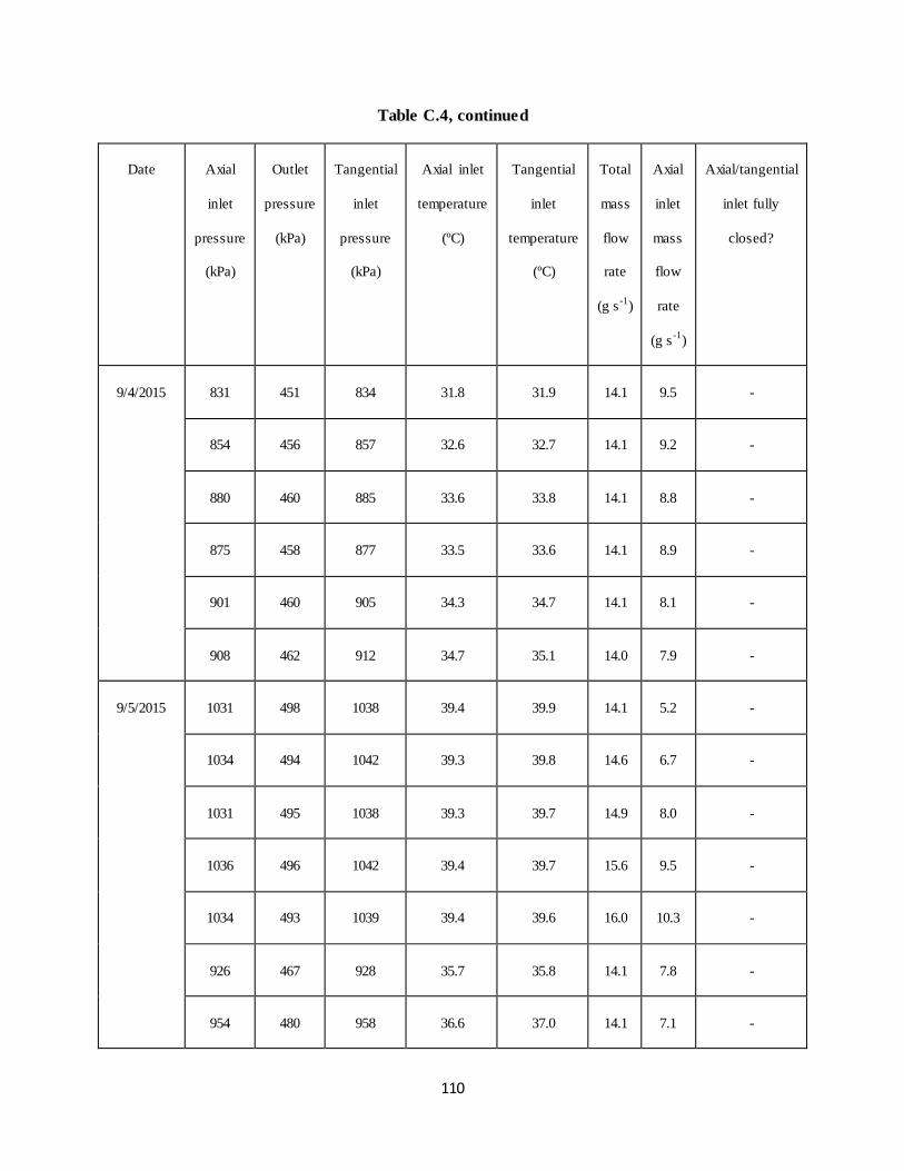
110
Table C.4, continued
Date Axial
inlet
pressure
(kPa)
Outlet
pressure
(kPa)
Tangential
inlet
pressure
(kPa)
Axial inlet
temperature
(ºC)
Tangential
inlet
temperature
(ºC)
Total
mass
flow
rate
(g s-1
)
Axial
inlet
mass
flow
rate
(g s-1
)
Axial/tangential
inlet fully
closed?
9/4/2015 831 451 834 31.8 31.9 14.1 9.5 -
854 456 857 32.6 32.7 14.1 9.2 -
880 460 885 33.6 33.8 14.1 8.8 -
875 458 877 33.5 33.6 14.1 8.9 -
901 460 905 34.3 34.7 14.1 8.1 -
908 462 912 34.7 35.1 14.0 7.9 -
9/5/2015 1031 498 1038 39.4 39.9 14.1 5.2 -
1034 494 1042 39.3 39.8 14.6 6.7 -
1031 495 1038 39.3 39.7 14.9 8.0 -
1036 496 1042 39.4 39.7 15.6 9.5 -
1034 493 1039 39.4 39.6 16.0 10.3 -
926 467 928 35.7 35.8 14.1 7.8 -
954 480 958 36.6 37.0 14.1 7.1 -
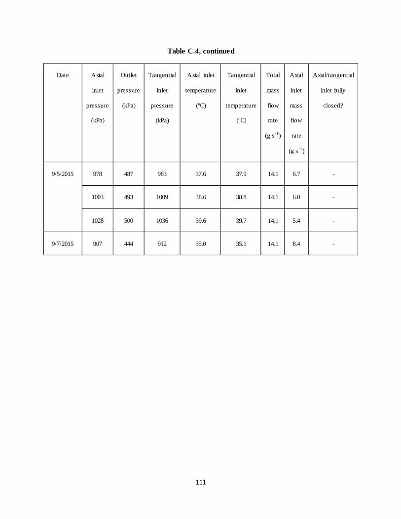
111
Table C.4, continued
Date Axial
inlet
pressure
(kPa)
Outlet
pressure
(kPa)
Tangential
inlet
pressure
(kPa)
Axial inlet
temperature
(ºC)
Tangential
inlet
temperature
(ºC)
Total
mass
flow
rate
(g s-1
)
Axial
inlet
mass
flow
rate
(g s-1
)
Axial/tangential
inlet fully
closed?
9/5/2015 978 487 983 37.6 37.9 14.1 6.7 -
1003 493 1009 38.6 38.8 14.1 6.0 -
1028 500 1036 39.6 39.7 14.1 5.4 -
9/7/2015 907 444 912 35.0 35.1 14.1 8.4 -