Embed Size (px)
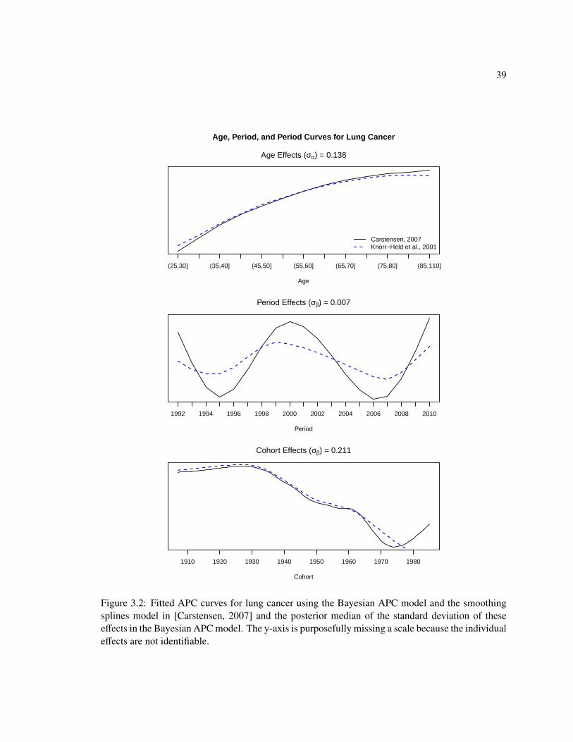
Citation preview

©Copyright 2014
Theresa R. Smith


Bayesian Spatial and Temporal Methods for Public Health Data
Theresa R. Smith
A dissertationsubmitted in partial fulfillment of the
requirements for the degree of
Doctor of Philosophy
University of Washington
2014
Reading Committee:
Adrian Dobra, Chair
Jonathan C Wakefield, Chair
Peter D Hoff
Program Authorized to Offer Degree:Statistics

University of Washington
Abstract
Bayesian Spatial and Temporal Methods for Public Health Data
Theresa R. Smith
Co-Chairs of the Supervisory Committee:Associate Professor Adrian Dobra
Department of Statistics
Professor Jonathan C WakefieldDepartment of Statistics
In this thesis, we develop flexible models to analyze public health data in time and/or in space. The
development of our methodology is motivated by two examples: cancer incidence data in Washing-
ton State and birth outcome data in North Carolina. First, we describe a temporal cancer incidence
model and demonstrate how to use this model to forecast incidence for future years, identify the
relevant time scales on which disease incidence changes, and estimate the effects of screening rates
and tobacco use on female breast cancer and male lung cancer. In the next chapter, we introduce the
negative G-Wishart prior for the covariance matrix of Gaussian spatial random effects. We show via
a simulation study that this new prior has advantages over the more rigid Gaussian Markov random
field (GMRF) priors, and we apply this new prior in a multivariate setting using the cancer incidence
data. Finally, we use binary trees together with graphical log-linear models to capture spatial inter-
actions as well as interactions between outcomes in sets of spatially dependent binary tables. This
approach is illustrated using the North Carolina data.


TABLE OF CONTENTS
Page
List of Figures . . . . . . . . . . . . . . . . . . . . . . . . . . . . . . . . . . . . . . . . . . iii
List of Tables . . . . . . . . . . . . . . . . . . . . . . . . . . . . . . . . . . . . . . . . . . v
Chapter 1: Introduction . . . . . . . . . . . . . . . . . . . . . . . . . . . . . . . . . . 1
1.1 Spatial Data . . . . . . . . . . . . . . . . . . . . . . . . . . . . . . . . . . . . . . 1
1.2 Bayesian Models for Spatially Aggregated Health Data . . . . . . . . . . . . . . . 2
1.3 Motivating Examples . . . . . . . . . . . . . . . . . . . . . . . . . . . . . . . . . 3
1.4 Structure of the Thesis . . . . . . . . . . . . . . . . . . . . . . . . . . . . . . . . 11
Chapter 2: Review of Statistical Methods . . . . . . . . . . . . . . . . . . . . . . . . 14
2.1 Graphical Models . . . . . . . . . . . . . . . . . . . . . . . . . . . . . . . . . . . 14
2.2 Gaussian Markov Random Fields . . . . . . . . . . . . . . . . . . . . . . . . . . . 16
2.3 Bayesian Computation . . . . . . . . . . . . . . . . . . . . . . . . . . . . . . . . 21
Chapter 3: Temporal Models for Cancer Incidence in Washington State . . . . . . . . 26
3.1 Introduction . . . . . . . . . . . . . . . . . . . . . . . . . . . . . . . . . . . . . . 26
3.2 Temporal Models for Cancer Incidence . . . . . . . . . . . . . . . . . . . . . . . 28
3.3 A Bayesian APC Model . . . . . . . . . . . . . . . . . . . . . . . . . . . . . . . . 33
3.4 The APC Model for Breast Cancer and Lung Cancer . . . . . . . . . . . . . . . . 38
3.5 Incorporating Covariates in the APC model . . . . . . . . . . . . . . . . . . . . . 45
3.6 Results of the Aggregate Regression Models . . . . . . . . . . . . . . . . . . . . . 52
3.7 Discussion and Conclusions . . . . . . . . . . . . . . . . . . . . . . . . . . . . . 56
Chapter 4: Restricted Covariance Priors For Spatial Random Effects . . . . . . . . . . 59
4.1 Introduction . . . . . . . . . . . . . . . . . . . . . . . . . . . . . . . . . . . . . . 59
4.2 Background . . . . . . . . . . . . . . . . . . . . . . . . . . . . . . . . . . . . . . 60
4.3 Methods . . . . . . . . . . . . . . . . . . . . . . . . . . . . . . . . . . . . . . . . 63
4.4 Simulation . . . . . . . . . . . . . . . . . . . . . . . . . . . . . . . . . . . . . . . 70
i

4.5 Multiple Disease Mapping . . . . . . . . . . . . . . . . . . . . . . . . . . . . . . 754.6 Discussion . . . . . . . . . . . . . . . . . . . . . . . . . . . . . . . . . . . . . . . 77
Chapter 5: Bayesian Methods for Sets of Binary Contingency Tables . . . . . . . . . . 815.1 Introduction . . . . . . . . . . . . . . . . . . . . . . . . . . . . . . . . . . . . . . 815.2 Natural Exponential Family for Binary Contingency Tables . . . . . . . . . . . . . 845.3 Bayesian Inference for Binary Tables . . . . . . . . . . . . . . . . . . . . . . . . . 875.4 Extending to Sets of Tables . . . . . . . . . . . . . . . . . . . . . . . . . . . . . . 925.5 Combining Trees with Log-linear Models . . . . . . . . . . . . . . . . . . . . . . 995.6 Example . . . . . . . . . . . . . . . . . . . . . . . . . . . . . . . . . . . . . . . . 1045.7 Discussion . . . . . . . . . . . . . . . . . . . . . . . . . . . . . . . . . . . . . . . 109
Chapter 6: Discussion and Future Work . . . . . . . . . . . . . . . . . . . . . . . . . 113
Appendix A: Supplement to Chapter 3 . . . . . . . . . . . . . . . . . . . . . . . . . . . 128A.1 INLA versus MCMC . . . . . . . . . . . . . . . . . . . . . . . . . . . . . . . . . 128A.2 Forecasts . . . . . . . . . . . . . . . . . . . . . . . . . . . . . . . . . . . . . . . 131
Appendix B: Supplement to Chapter 4 . . . . . . . . . . . . . . . . . . . . . . . . . . . 139B.1 Proof of Theorem 1 . . . . . . . . . . . . . . . . . . . . . . . . . . . . . . . . . . 139B.2 Prior Selection for α and τ2 . . . . . . . . . . . . . . . . . . . . . . . . . . . . . 141B.3 Sampler Details . . . . . . . . . . . . . . . . . . . . . . . . . . . . . . . . . . . . 142B.4 Additional Figures . . . . . . . . . . . . . . . . . . . . . . . . . . . . . . . . . . 142
ii

LIST OF FIGURES
Figure Number Page
1.1 Pairwise scatter plots for log((y + 0.5)/E) in 2010. . . . . . . . . . . . . . . . . . 7
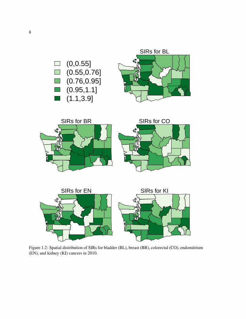
1.2 Spatial distribution of SIRs for bladder, breast, colorectal, endomitrium, and kidneycancers in 2010. . . . . . . . . . . . . . . . . . . . . . . . . . . . . . . . . . . . . 8
1.3 Spatial distribution of SIRs for leukemia, lung cancer, Non-Hodgkin lymphoma,melanoma of the skin, and prostate cancer in 2010. . . . . . . . . . . . . . . . . . 9
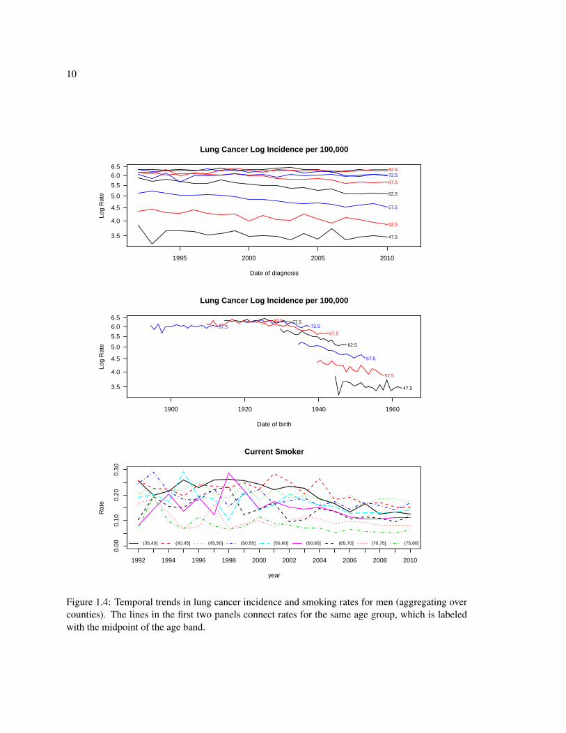
1.4 Lung cancer and smoking rates . . . . . . . . . . . . . . . . . . . . . . . . . . . . 10
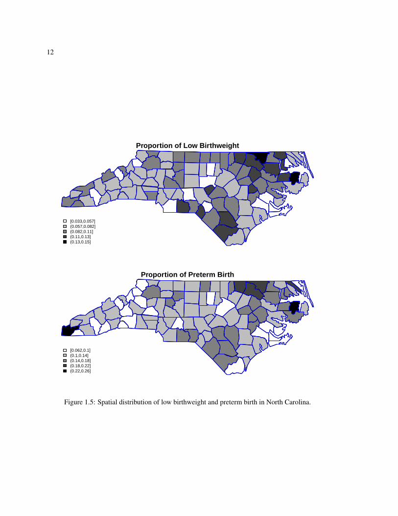
1.5 Low Birthweight and Preterm Birth Rates . . . . . . . . . . . . . . . . . . . . . . 12
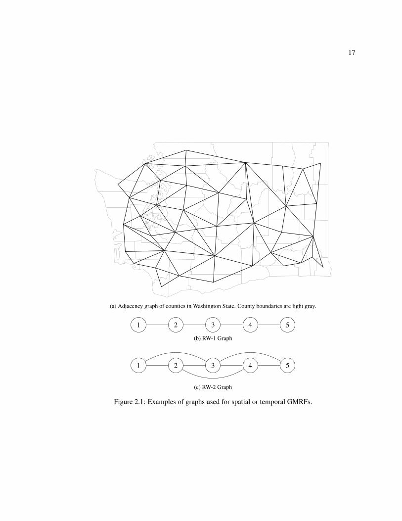
2.1 Example GMRF graphs . . . . . . . . . . . . . . . . . . . . . . . . . . . . . . . . 17
2.2 RW-1 versus RW-2 fit . . . . . . . . . . . . . . . . . . . . . . . . . . . . . . . . . 20
3.1 Fitted APC curves for breast cancer . . . . . . . . . . . . . . . . . . . . . . . . . 37
3.2 Fitted APC curves for lung cancer . . . . . . . . . . . . . . . . . . . . . . . . . . 39
3.3 Fitted versus observed log rates for breast cancer . . . . . . . . . . . . . . . . . . 44
3.4 Fitted versus observed log rates for lung cancer . . . . . . . . . . . . . . . . . . . 46
3.5 Smoking rates by age and year . . . . . . . . . . . . . . . . . . . . . . . . . . . . 50
3.6 Mammography rates by age and year . . . . . . . . . . . . . . . . . . . . . . . . . 53
3.7 Log relative risks due to mammograms by age. . . . . . . . . . . . . . . . . . . . 57
4.1 Expected counts for simulation study . . . . . . . . . . . . . . . . . . . . . . . . . 71
4.2 Labels (Li) for simulation study . . . . . . . . . . . . . . . . . . . . . . . . . . . 72
4.3 Root average mean squared error (RAMSE) for relative risks θ . . . . . . . . . . . 74
4.4 Posterior distribution of the spatial autocorrelation parameter ρ under the five mod-els considered. . . . . . . . . . . . . . . . . . . . . . . . . . . . . . . . . . . . . . 78
4.5 Pairwise edge inclusion probabilities for GC . . . . . . . . . . . . . . . . . . . . . 79
5.1 Cut rule based on distance. . . . . . . . . . . . . . . . . . . . . . . . . . . . . . . 96
5.2 Samples from the pinball prior . . . . . . . . . . . . . . . . . . . . . . . . . . . . 97
5.3 Prior co-membership by graph distance . . . . . . . . . . . . . . . . . . . . . . . 98
5.4 Log posterior probability with and without restarts . . . . . . . . . . . . . . . . . 104
5.5 Prior versus posterior co-membership by graph distance . . . . . . . . . . . . . . . 108
iii

5.6 Graphs based on thresholding the posterior probability of edge inclusion. . . . . . 1095.7 Posterior mean for the odds ratio of preterm birth for smokers and non smokers. . . 1105.8 Maternal education and smoking. . . . . . . . . . . . . . . . . . . . . . . . . . . . 110
A.1 Comparison of fitted log rates and random effects for the breast cancer AP model. . 129A.2 Comparison of fitted log rates and random effects for the breast cancer AP model. . 130A.3 Forecasts versus observed values for the four APC models for breast and lung cancer. 132A.4 Breast cancer forecasts for the 25–50 age groups using the AP model. . . . . . . . 133A.5 Breast cancer forecasts for the 50–75 age groups using the AP model. . . . . . . . 134A.6 Breast cancer forecasts for the 75+ age groups using the AP model. . . . . . . . . 135A.7 Lung cancer forecasts for the 25–50 age groups using the AC model. . . . . . . . . 136A.8 Lung cancer forecasts for the 50–75 age groups using the AC model. . . . . . . . . 137A.9 Lung cancer forecasts for the 75+ age groups using the AC model. . . . . . . . . . 138
B.1 Mixing for estimates of the ratio of normalizing constants. . . . . . . . . . . . . . 143B.2 Mixing for the Cholesky square root in the univariate simulations. . . . . . . . . . 144B.3 Mixing for random effects in the univariate simulations . . . . . . . . . . . . . . . 145B.4 SIRs versus smoothed estimates for all cancers . . . . . . . . . . . . . . . . . . . 146B.5 SIRs versus smoothed estimates for two counties . . . . . . . . . . . . . . . . . . 147
iv

LIST OF TABLES
Table Number Page
1.1 Summary statistics for Washington State incidence data . . . . . . . . . . . . . . . 6
3.1 APC indices. . . . . . . . . . . . . . . . . . . . . . . . . . . . . . . . . . . . . . 293.2 APC forecast indices. . . . . . . . . . . . . . . . . . . . . . . . . . . . . . . . . . 323.3 Total incidence by age band. . . . . . . . . . . . . . . . . . . . . . . . . . . . . . 363.4 Total incidence by year. . . . . . . . . . . . . . . . . . . . . . . . . . . . . . . . . 383.5 Comparison of models for breast cancer rates. . . . . . . . . . . . . . . . . . . . . 423.6 Posterior medians for the overall log rate and variance components for breast cancer. 423.7 Comparison of models for lung cancer rates . . . . . . . . . . . . . . . . . . . . . 433.8 Posterior medians for the overall log rate and variance components for lung cancer. 453.9 Comparison of aggregate and ecological models for breast cancer . . . . . . . . . . 543.10 Comparison of aggregate and ecological models lung cancer . . . . . . . . . . . . 55
4.1 Ten-fold cross validation results for multivariate disease mapping with WashingtonState cancer incidence data . . . . . . . . . . . . . . . . . . . . . . . . . . . . . . 76
4.2 Coverage rates and mean lengths of in-sample 95% credible intervals. . . . . . . . 77
5.1 MSE results for LBW-RACE . . . . . . . . . . . . . . . . . . . . . . . . . . . . . 1075.2 MSE results for full (25) tables . . . . . . . . . . . . . . . . . . . . . . . . . . . . 1075.3 MSE results for 25 models for different tree priors . . . . . . . . . . . . . . . . . . 107
A.1 Comparison of posterior medians for the breast AP model. . . . . . . . . . . . . . 128A.2 Comparison of posterior medians for the lung AC model. . . . . . . . . . . . . . . 128
B.1 Ten-fold cross validation results for ρ = 0.99 . . . . . . . . . . . . . . . . . . . . 148B.2 Ten-fold cross validation results when ρ = 0.9 . . . . . . . . . . . . . . . . . . . . 148B.3 Ten-fold cross validation results for π(ρ) is U{0.05, 0.1, 0.15, . . . , 0.85, 0.9, 0.95, 0.99}148
v

ACKNOWLEDGMENTS
This thesis would not have been possible without the contributions and support of many people.
First, I would like to thank my advisors Adrian Dobra and Jon Wakefield. Adrian first introduced
me to spatial statistics, statistical computing, and graphical models. He has been one of my most
important teachers and collaborators. Jon sparked my interest in epidemiological applications and
has pushed me to become a better writer and researcher. He has been a great mentor and friend.
I would also like to thank my committee members: Peter Hoff, Emily Fox, and Chris Simpson.
Their thoughtful comments have improved this work and have generated many ideas for future
research. Abel Rodriguez, Laina Mercer, and Håvard Rue have provided invaluable computational
help as well as many interesting discussions.
The entire faculty and staff of the Statistics Department were an important part of this work.
Classes and discussions with faculty members have strengthened my understanding of and love for
the field of statistics. The enthusiastic assistance of staff members when navigating the policies and
procedures of the university ensured that I could focus on my research.
My fellow students have been a constant source of support, both academically and personally
over the past five years. I owe an extra helping of gratitude to Jan Irvahn, Rebecca Ferrell, and Alex
Volfovsky for the conversation, advice, and comic relief they’ve provided, even from afar.
Finally, I would like to thank my family. To my parents and siblings: thank you for your endless
encouragement and optimism. And to my husband, Steven, thank you for your faith in me and
seemingly infinite patience. Your love, support, and sacrifice are the foundation of this work.
vi

DEDICATION
In memory of
G. Alec ‘Doc’ Stewart
1941-2010
vii


1
Chapter 1
INTRODUCTION
1.1 Spatial Data
Spatial data arise when outcomes and predictors of interested are observed at particular points or
regions inside a defined study area. Spatial data sets are common in many fields including environ-
mental science, economics, public health, and epidemiology. In epidemiology, understanding the
underlying spatial patterns of a disease is an important starting point for further investigations. Be-
yond this, determining the association between risk measures and spatially indexed covariates such
as environmental pollutants is clearly of interest. Key goals in public health are to understand what
factors contribute to increased incidence or mortality of diseases and to allocate resources based on
predictions of the future burden of these diseases.
The risk of disease inherently varies in space because risk factors are non-uniformly distributed
in space. Such risk factors may include demographic characteristics (such as race and age structure),
socioeconomic factors (such as income level), or exposure levels of environmental causes of disease
(such as air pollution or UV radiation). While information is sometimes available about known risk
factors, we often use statistical models to account for unobserved risk factors. The questions posed
by epidemiologists and public heath officials fall into three broad categories:
1. Descriptive: What is the distribution of disease risk in the study region? Are there any notice-
able trends or irregularities?
2. Inferential: Is disease risk associated with measured covariates? Are the observed irregu-
larities in the spatial pattern of disease risk actual clusters or do they just reflect sampling
variability?
3. Predictive: How many cases of a disease can we expect in the future?
2
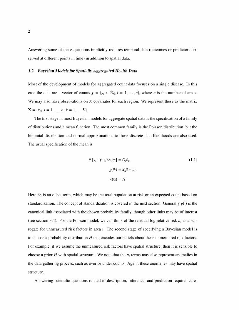
Answering some of these questions implicitly requires temporal data (outcomes or predictors ob-
served at different points in time) in addition to spatial data.
1.2 Bayesian Models for Spatially Aggregated Health Data
Most of the development of models for aggregated count data focuses on a single disease. In this
case the data are a vector of counts y = {yi ∈ N0, i = 1, . . . , n}, where n is the number of areas.
We may also have observations on K covariates for each region. We represent these as the matrix
X = {xik, i = 1, . . . , n; k = 1, . . .K}.
The first stage in most Bayesian models for aggregate spatial data is the specification of a family
of distributions and a mean function. The most common family is the Poisson distribution, but the
binomial distribution and normal approximations to these discrete data likelihoods are also used.
The usual specification of the mean is
E[yi | y−i,Oi, ηi
]= Oiθi, (1.1)
g(θi) = x′iβ + ui,
π(u) = H
Here Oi is an offset term, which may be the total population at risk or an expected count based on
standardization. The concept of standardization is covered in the next section. Generally g(·) is the
canonical link associated with the chosen probability family, though other links may be of interest
(see section 3.4). For the Poisson model, we can think of the residual log relative risk ui as a sur-
rogate for unmeasured risk factors in area i. The second stage of specifying a Bayesian model is
to choose a probability distribution H that encodes our beliefs about these unmeasured risk factors.
For example, if we assume the unmeasured risk factors have spatial structure, then it is sensible to
choose a prior H with spatial structure. We note that the ui terms may also represent anomalies in
the data gathering process, such as over or under counts. Again, these anomalies may have spatial
structure.
Answering scientific questions related to description, inference, and prediction requires care-

3
ful estimation of θ and quantifying our uncertainty about these estimates. For rare outcomes, such
as rare cancers, the observed counts can be highly variable in regions with small populations, and
careful estimation of the residuals u is even more crucial. Much of the previous development of sta-
tistical models for areal data has focused on specifying H so that we can smooth out the uncertainty
in the relative risk estimates by sharing strength among neighboring areas.
1.3 Motivating Examples
Recent research has focused on extending models for single diseases to multivariate settings. We
may observe counts of the same disease over T time points, we may have counts for p related
diseases over the same study region, or we may wish to avoid aggregation over demographic groups
such as race and age. In this dissertation, we propose new flexible choices for H as well as extensions
of univariate disease mapping approaches to multi-way and multivariate data. We use two datasets
in this thesis and base several simulation studies on the spatial structure in these data. In chapters 3
and 4 we use cancer incidence data from Washington State, and in chapter 5, we use birth outcome
data from North Carolina.
1.3.1 Cancer Incidence in Washington State
We use incidence data from the Washington State Cancer Registry (WSCR) for developing univari-
ate and multivariate disease mapping methods. WSCR contains all reported incident cases of in situ
and invasive cancers from 1992 to 2010. There are just over 590, 000 cases with between 24, 000
and 37, 000 cases each year. These data are individual records reported by health care workers
and health care facilities to either the State Cancer Registry directly or via the Cancer Surveillance
System at the Fred Hutchinson Cancer Research Center for those cases originating in the Puget
Sound area. The records contain information about age, sex, race, ethnicity, county of residence
at diagnosis, year of diagnosis and cancer type. Cancer type is initially available as ICD-02 codes
(1992–1998) or ICD-03 codes (1999–2010) and histology codes, but for the top 26 cancers, these
codes are grouped into colloquially recognized cancer types (e.g., breast cancer or colon cancer).
Aggregating over demographic groups, we can represent the data as a 39 × 19 × 26 array, where 39

4
is the number of counties in Washington State and 19 is the number of years. The entries in this
array range from 0 to just under 2000.
We combine the cancer registry data with demographic and behavioral data. We retrieved pop-
ulation for each every year (1992–2010), county, gender, quintenial age band, and race (white, non
Hispanic or non-white) combination from the National Center for Health Statistics (NCHS [2012]).
The data are based on intercensal estimates of the July 1 population based on information on migra-
tion, births, and deaths available from the Federal-State Cooperative for Population Estimates, the
Internal Revenue Service, and the Social Security administration. Demographic data from the 90s
are processed to account for changes brought on by a 1997 law that created separate categories for
Asian and Pacific Islanders and allowed for people to belong to multiple race categories. Ingram
et al. [2003] have developed logistic regression models to predict the primary race of respondents in
an effort to make pre-1997 and post-1997 data sources compatible. These post processed race data
are known as “bridged race” categories. WSCR constructs bridged race in a similar fashion.
We use these population estimates to construct offsets as in equation (1.1). If the observed
counts are aggregated over demographic groups such as sex, age, and race, then expected counts are
generally included as an offset to the mean model to account for differences in disease risk due to
differences in the demographic composition of each area. Suppose q j is the rate of disease within
demographic group j and Pi j is the population of area i in demographic group j. Then Ei is the
expected count for area i and is calculated as
Ei =
J∑j=1
q jPi j. (1.2)
We can use previously published estimates for q j or, if the observed counts are available for each
demographic group, we can estimate q j from the data. If the rates are calculated using the same
data we intend to analyze, then the expected counts are known as internally standardized. If yi j is
the observed number of cases in area i and demographic group j, then the internally standardized

5
expected counts are
Ei =
J∑j=1
Pi j
∑nk=1 yk j∑nk=1 Pk j
. (1.3)
The ratio of the observed count to the expected count is called the standardized incidence or mor-
tality ratio (depending on whether the data are counts of incident cases or deaths). The standardized
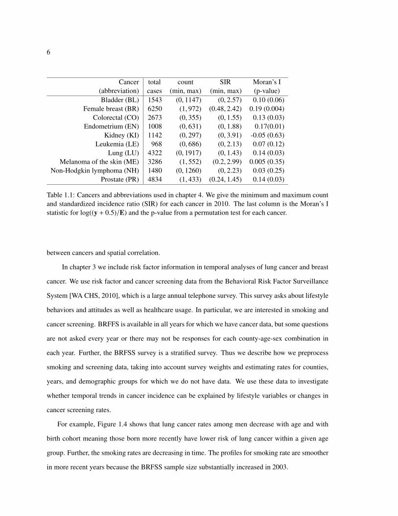
incidence ratio is the maximum likelihood estimator of the relative risk in each area. Table 1.1 shows
summaries for SIRs of the top ten cancers (based on overall incidence) in 2010. The expected counts
are based on age and gender rates estimated from the entire cancer registry. We use this particular
subset of the cancer registry data in chapter 4. There are zero counts and therefore zero-valued SIRs
as well as some large SIRs. For example, the maximum SIR of 3.91 means that for that county, the
number of cases of kidney cancer was nearly four times higher than expected.
Moran’s I is one measure of spatial autocorrelation that uses the neighborhood structure of the
study region, and it is on the same scale as ordinary correlation [Moran, 1950]. For a vector x with
sample mean x and for a weights matrix W = {wi j, i, j = 1, . . . , n}, Moran’s I is
I =n∑n
i=1∑n
j=1 wi j
∑ni=1
∑nj=1 wi j(xi − x)(x j − x)∑n
i=1(xi − x)2 .
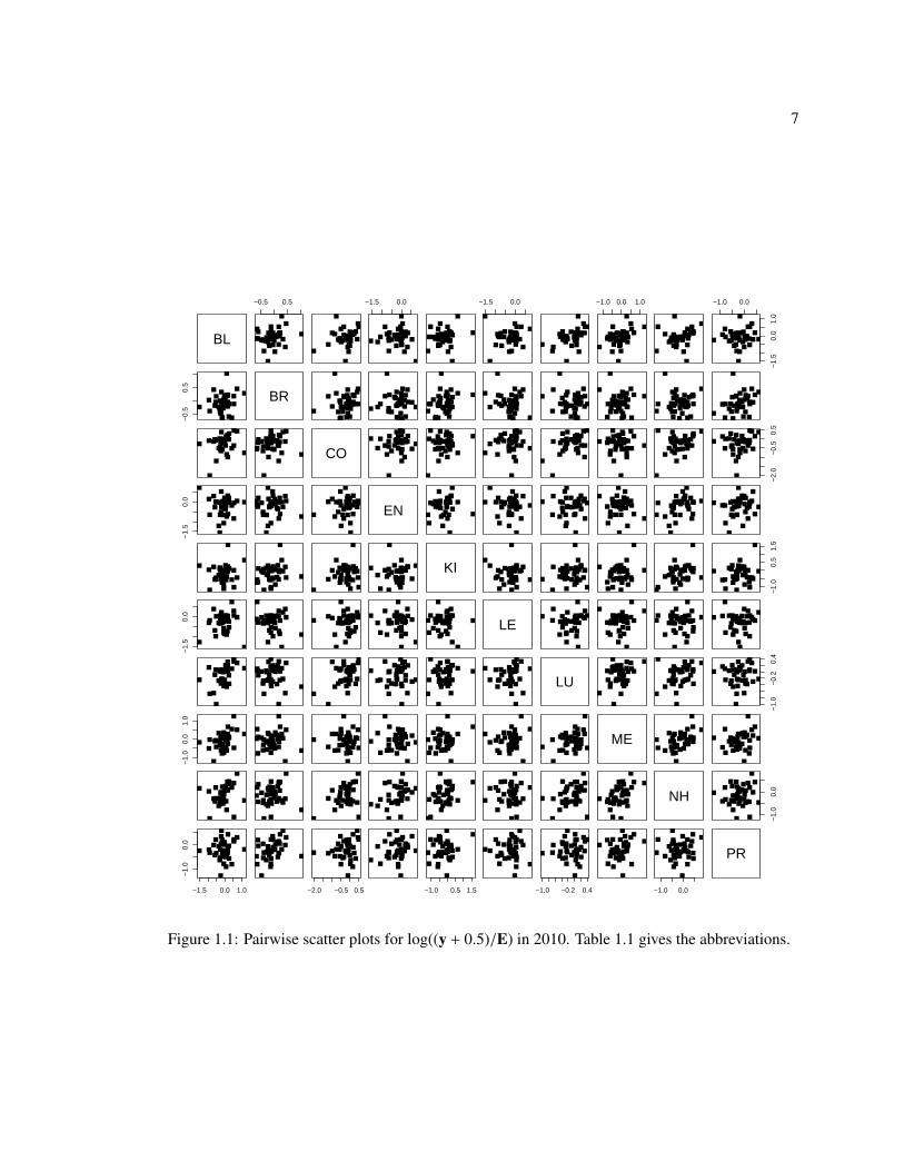
We use the inverse distance between county centroids as weights, wi j and xi = log((yi + 0.5)/Ei).
We use the log transformation to decrease the impact of the large SIRs on the correlation estimates
and to have an outcome that is less heteroscedastic than the original SIRs. Adjusting the number of
cases by adding 0.5 avoids numerical issues and is equivalent to the posterior mean for θi under the
Jeffry’s prior π(θi) ∝ θ−1/2. We test whether Moran’s I is different from zero for each cancer using
a permutation test that permutes the log adjusted SIRs across counties. The observed Moran’s I
statistic is then compared to the empirical distribution. For most of the cancers, there is evidence of
positive spatial correlation in the log adjusted SIRs. Figures 1.1, 1.2, and 1.3 show the relationships
between the log SIRs for each pair of cancers and the spatial distribution of the SIRs for each cancer.
In chapter 4 we propose a new model that flexibly models both sources of correlation: correlation
6
Cancer total count SIR Moran’s I(abbreviation) cases (min, max) (min, max) (p-value)Bladder (BL) 1543 (0, 1147) (0, 2.57) 0.10 (0.06)
Female breast (BR) 6250 (1, 972) (0.48, 2.42) 0.19 (0.004)Colorectal (CO) 2673 (0, 355) (0, 1.55) 0.13 (0.03)
Endometrium (EN) 1008 (0, 631) (0, 1.88) 0.17(0.01)Kidney (KI) 1142 (0, 297) (0, 3.91) -0.05 (0.63)
Leukemia (LE) 968 (0, 686) (0, 2.13) 0.07 (0.12)Lung (LU) 4322 (0, 1917) (0, 1.43) 0.14 (0.03)
Melanoma of the skin (ME) 3286 (1, 552) (0.2, 2.99) 0.005 (0.35)Non-Hodgkin lymphoma (NH) 1480 (0, 1260) (0, 2.23) 0.03 (0.25)
Prostate (PR) 4834 (1, 433) (0.24, 1.45) 0.14 (0.03)
Table 1.1: Cancers and abbreviations used in chapter 4. We give the minimum and maximum countand standardized incidence ratio (SIR) for each cancer in 2010. The last column is the Moran’s Istatistic for log((y + 0.5)/E) and the p-value from a permutation test for each cancer.
between cancers and spatial correlation.
In chapter 3 we include risk factor information in temporal analyses of lung cancer and breast
cancer. We use risk factor and cancer screening data from the Behavioral Risk Factor Surveillance
System [WA CHS, 2010], which is a large annual telephone survey. This survey asks about lifestyle
behaviors and attitudes as well as healthcare usage. In particular, we are interested in smoking and
cancer screening. BRFFS is available in all years for which we have cancer data, but some questions
are not asked every year or there may not be responses for each county-age-sex combination in
each year. Further, the BRFSS survey is a stratified survey. Thus we describe how we preprocess
smoking and screening data, taking into account survey weights and estimating rates for counties,
years, and demographic groups for which we do not have data. We use these data to investigate
whether temporal trends in cancer incidence can be explained by lifestyle variables or changes in
cancer screening rates.
For example, Figure 1.4 shows that lung cancer rates among men decrease with age and with
birth cohort meaning those born more recently have lower risk of lung cancer within a given age
group. Further, the smoking rates are decreasing in time. The profiles for smoking rate are smoother
in more recent years because the BRFSS sample size substantially increased in 2003.
7
BL
−0.5 0.5 −1.5 0.0 −1.5 0.0 −1.0 0.0 1.0 −1.0 0.0
−1.
50.
01.
0
−0.
50.
5
BR
CO
−2.
0−
0.5
0.5
−1.
50.
0
EN
KI
−1.
00.
51.
5
−1.
50.
0
LE
LU
−1.
0−
0.2
0.4
−1.
00.
01.
0
ME
NH
−1.
00.
0
−1.5 0.0 1.0
−1.
00.
0
−2.0 −0.5 0.5 −1.0 0.5 1.5 −1.0 −0.2 0.4 −1.0 0.0
PR
Figure 1.1: Pairwise scatter plots for log((y + 0.5)/E) in 2010. Table 1.1 gives the abbreviations.
8
(0,0.55](0.55,0.76](0.76,0.95](0.95,1.1](1.1,3.9]
SIRs for BL
SIRs for BR SIRs for CO
SIRs for EN SIRs for KI
Figure 1.2: Spatial distribution of SIRs for bladder (BL), breast (BR), colorectal (CO), endomitrium(EN), and kidney (KI) cancers in 2010.

9
(0,0.55](0.55,0.76](0.76,0.95](0.95,1.1](1.1,3.9]
SIRs for LE
SIRs for LU SIRs for ME
SIRs for NH SIRs for PR
Figure 1.3: Spatial distribution of SIRs for leukemia (LE), lung cancer (LU), Non-Hodgkin lym-phoma (NH), melanoma of the skin (ME), and prostate cancer (PR) in 2010.
10
1995 2000 2005 2010
3.5
4.0
4.5
5.0
5.5
6.06.5
Date of diagnosis
Log
Rat
e
47.5
52.5
57.5
62.5
67.5
72.5 82.5
Lung Cancer Log Incidence per 100,000
1900 1920 1940 1960
3.5
4.0
4.5
5.0
5.5
6.06.5
Date of birth
Log
Rat
e
47.5
52.5
57.5
62.5
67.5
72.5 77.5 82.5
97.5
Lung Cancer Log Incidence per 100,000
Current Smoker
year
Rat
e
1992 1994 1996 1998 2000 2002 2004 2006 2008 2010
0.00
0.10
0.20
0.30
(35,40] (40,45] (45,50] (50,55] (55,60] (60,65] (65,70] (70,75] (75,80]
Figure 1.4: Temporal trends in lung cancer incidence and smoking rates for men (aggregating overcounties). The lines in the first two panels connect rates for the same age group, which is labeledwith the midpoint of the age band.

11
1.3.2 Birth records in North Carolina
In chapter 5 we consider records of all live births recorded in North Carolina in 2006 [NC SCHS,
2007] with a goal of understanding the relationships between two adverse birth outcomes and how
these relationships might vary spatially. We use the same five binary variables used by Tassone et al.
[2010]: low birthweight (1–less than 2500 grams, 2–at least 2500 grams), full term birth (1–less than
37 weeks gestational age, 2–at least 37 weeks), maternal race (1–white/non Hispanic, 2–black/non
Hispanic), infant sex (1–male, 2–female), and maternal smoking (1–non smoker, 2–smoker). The
smoker-non smoker outcome is determined from self reported number of cigarettes used daily. To
eliminate those records for which there is a known physiological explanation for low birthweight or
preterm birth, we exclude infants with congenital defects and multiple births. Further, we limit our
data to mothers between 15 and 44 years of age who are white/non Hispanic or black/non Hispanic.
The data consist of 96, 046 individual records, each associated with one of 100 counties based on
the mother’s residence. We can regard the data as 100 separate 25 contingency tables, with table
totals ranging from 39 to 9850. There are a substantial number of sampling zeros (713) and counts
less than 3 (1390) in these tables.
Figure 1.5 shows the proportion of low birthweight and preterm birth by county for these data.
For both adverse outcomes, there are higher proportions in several northeastern and southeastern
counties. Overall, preterm birth is more common than low birthweight, with state wide rates of
12.1% for preterm birth versus 7.7% for low birthweight. In chapter 5 we develop a joint model for
these adverse birth outcomes that allows for spatial heterogeneity in the strengths of associations
between outcomes and risk factors as well as spatial heterogeneity in the interaction model.
1.4 Structure of the Thesis
In this thesis, we aim to develop more flexible models for spatial dependence and for interactions
between risk factors and outcomes in our two motivating examples. In chapter 2, we review the
statistical tools that we will use in later chapters. These tools include graphical models, Gaussian
Markov random fields (GMRFs), and Bayesian computation techniques. In chapter 3 we introduce
12
[0.033,0.057](0.057,0.082](0.082,0.11](0.11,0.13](0.13,0.15]
Proportion of Low Birthweight
[0.062,0.1](0.1,0.14](0.14,0.18](0.18,0.22](0.22,0.26]
Proportion of Preterm Birth
Figure 1.5: Spatial distribution of low birthweight and preterm birth in North Carolina.

13
temporal models for cancer incidence and demonstrate forecasting from these models. We also
derive an aggregate model for estimating individual exposure effects in the temporal model using
survey data on cancer screening and tobacco use. In Chapter 4 we introduce a prior for restricted
covariance matrices and illustrate the application of this prior in the context of Gaussian spatial
random effects. We show via a simulation study that this new prior has advantages over the more
rigid GMRF priors, and we use this new prior in a multivariate setting using the cancer incidence
data. In chapter 5 we develop a spatial clustering prior for sets of multi-way contingency tables. We
use binary trees together with graphical log-linear models to capture spatial interactions as well as
interactions between outcomes. We fit this new model to the birth records data in North Carolina.
Finally in chapter 6 we discuss directions for future research.

14
Chapter 2
REVIEW OF STATISTICAL METHODS
2.1 Graphical Models
Graphical models define families of probability distributions over a random vector x. Within each
family, the probability distributions share a conditional independence structure defined by an undi-
rected graph. Among other things, graphical models are used to represent beliefs or learn about
relationships in data as well as to factorize likelihoods for more efficient computation and estima-
tion.
An undirected graph consists of a set of vertices V and edges E: G = (V, E). The vertices repre-
sent the individual random variables in the vector x. In this thesis, we sometimes refer to E as a list
and sometimes as a binary matrix. That is if there is an edge between variables x1 and x2, we can
say either (1, 2) ∈ E or E[1, 2] = 1. Because G is undirected, (1, 2) ∈ E ⇐⇒ (2, 1) ∈ E. These
edges define a set of conditional independence or Markov relationships between subsets of V .
Let capital letters represent subsets of V and lowercase letters represent individual elements of
V . Let cl(a) be the closure of a, which consists of a and any neighbors of a, and nb(a) the set of
neighbors of a (the vertices connected to a by an edge). A set S separates A from B if the path from
any node in A to any node in B has to go through a node in S . There are three equivalent expressions
of these Markov properties [Lauritzen, 1996]:
• The pairwise Markov property For any pair (a, b) ∈ V and (a, b) < E: a ⊥⊥ b | V\{a, b}.
• The local Markov property For any a ∈ V: a ⊥⊥ V\cl(a) | nb(a).
• The global Markov property For any triple of disjoint subsets (A, B, S ) with S separating A
and B: A ⊥⊥ B | S .
Each of the above definitions has a corresponding expression as a constraint on the probability
family. For example let qA(xA) be a density function and qA|S (A | S ) be a conditional density

15
function. Then the third statement above implies
qAB|S (xA∪B | xS ) = qA|S (xA | xS )qB|S (xB | xS )
for any values of xS . When these densities are well defined and in particular if x is a discrete random
factor, we can rewrite this as
qABS (xA∪B∪S ) =qAS (xAS )qBS (xBS )
qS (xS ).
If a probability distribution measure P obeys the global Markov property for all choices of
A, B, and S , then that this measure is Markov with respect to the graph and we write P ∈ M(G)
[Dawid and Lauritzen, 1993]. The collection of all such probability models is called the graphical
model. In this thesis we use two kinds of graphical models, Gaussian graphical models and graphical
models for multi-way contingency tables. Both are parametric models, and we can express the set
M(G) through restrictions on the parameter space. For parametric probability families, we define
ΘG = {θ : Pθ ∈ M(G)}. As we will see in chapter 4, in a mean-zero Gaussian graphical model, θ is
the precision matrix and ΘG is the set of positive definite matrices with zeros in the elements that
correspond to missing edges in E.
In the Bayesian framework, we use prior distributions on the parameter space to incorporate our
beliefs. In the parametric, graphical model setting, these priors should have support only over ΘG.
Priors over the space of probability distributions that are Markov with respect to a graph are called
hyper Markov distributions [Dawid and Lauritzen, 1993]. In chapters 4 and 5, we give examples of
conjugate priors that are hyper Markov for Gaussian graphical models and for contingency tables.

16
2.2 Gaussian Markov Random Fields
In principle, a Gaussian Markov random field (GMRF) is no different from a Gaussian graphical
model. That if x = {x1, x2, . . . , xn} is a GMRF with respect to a graph G, then the density of x is
π(x) =|Q|1/2
(2π)n/2 exp(−12
(x − µ)T Q(x − µ)),
for Q positive definite with Qi j = 0 when (i, j) < E. When x are random effects in a spatial model,
the graph G is the adjacency graph of the study region. The indices i represent distinct areas, and
(i, j) ∈ E if areas i and j share a boundary. Firgure 2.1(a) gives an example of such a graph. If x
are random effects in a time series application, then G is often a line graph with (i, i + 1) ∈ E for
i = 1, . . . , n − 1 and potentially (i, i + 2) ∈ E for i = 1, . . . , n − 2. Two examples of these kinds of
graphs are shown in Figure 2.1(b) and (c).
The most common type of GMRF used in spatial statistics is a conditional autoregression
model or CAR model, which was first proposed by Besag [1974]. CAR models differ from Gaussian
graphical models because Q is defined implicitly through a set of n full conditional distributions.
For example, the conditional distribution for the random variable, xi, given the other variables, x−i,
is [Rue and Held, 2005]
xi | x−i ∼ N
µi +∑j: j,i
bi j(x j − µ j), τ2i
,with mean zero version
xi | x−i ∼ N
∑j: j,i
bi jx j, τ2i
.The joint distribution of the vector x is a mean zero multivariate normal distribution with precision
D−1(I − B), where Bi j = bi j, Bii = 0, and Dii = τ2i . Thus, to satisfy the Markov properties, bi j = 0
if (i, j) < E. This implied joint distribution is proper if D−1(I − B) is a symmetric, positive definite
matrix [Banerjee et al., 2004]. Symmetry is satisfied as long as bi j/τ2i = b ji/τ
2j , but satisfying the
17
(a) Adjacency graph of counties in Washington State. County boundaries are light gray.
1 2 3 4 5
(b) RW-1 Graph
1 2 3 4 5
(c) RW-2 Graph
Figure 2.1: Examples of graphs used for spatial or temporal GMRFs.

18
positive definite condition is less obvious. Thus, it is possible to specify a set of joint distributions
that do not give rise to a proper joint multivariate normal distribution.
The intrinsic conditional autoregression or ICAR prior is an example of this kind of distribution
and is the most commonly used prior for spatial random effects within the class of CAR priors.
Under the ICAR prior, the conditional mean for a given random effect is the weighted average of
the neighboring random effects, and the conditional variance is inversely proportion to the sum of
these weights:
xi | x−i ∼ N
1ωi+
∑j: j,i
ωi jx j,τ2
ωi+
.Here ωi j is nonzero if regions i and j are neighbors (i.e. share a border) and 0 otherwise, and
ωi+ is the sum of all of the weights for a specific area. The implied precision matrix for the joint
distribution is Q = τ−2(Dω −W) where Dω is a diagonal matrix with elements ωi+, i = 1, . . . n
and W = {ωi j; i , j, i, j = 1, . . . , n}. A binary specification for W is frequently used, though other
weights that incorporate the distance between areas can also be used [White and Ghosh, 2009]. In
the binary case, ωi j = 1 for neighboring regions and ωi+ = ni, the number of regions that border
area i. Under this specification, the conditional mean for a particular random effect is the average
value of the random effects for the neighboring regions, and the conditional variance is inversely
proportional to the number of neighbors of the area:
xi | x−i ∼ N
1ni
∑j∈nb(i)
x j,τ2
ni
. (2.1)
Besag et al. [1991] use a CAR prior for spatial random effects in a disease mapping context in
what has become known as the convolution model:
yi | Ei, θi ∼ Poi(Ei exp(θi)),
θi = xTi β + vi + ui.
19
Here vi is a non-spatial random effect and ui is a spatial random effect. The prior for v is N(0, σ2vI),
and the prior for u is the ICAR prior. We use this model as a competing method in chapter 4.
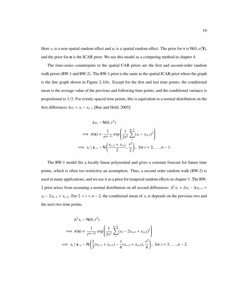
The time-series counterparts to the spatial CAR priors are the first and second-order random
walk priors (RW-1 and RW-2). The RW-1 prior is the same as the spatial ICAR prior where the graph
is the line graph shown in Figure 2.1(b). Except for the first and last time points, the conditional
mean is the average value of the previous and following time points, and the conditional variance is
proportional to 1/2. For evenly-spaced time points, this is equivalent to a normal distribution on the
first differences ∆xi = xi − xi−1 [Rue and Held, 2005]:
∆xi ∼ N(0, τ2)
=⇒ π(x) ∝1
τ(n−1) exp
12τ2
n−1∑i
(xi − xi+1)2
=⇒ xi | x−i ∼ N
(xi−1 + xi+1
2,τ2
2
), for i = 2, . . . , n − 1.
The RW-1 model fits a locally linear polynomial and gives a constant forecast for future time
points, which is often too restrictive an assumption. Thus, a second order random walk (RW-2) is
used in many applications, and we use it as a prior for temporal random effects in chapter 3. The RW-
2 prior arises from assuming a normal distribution on all second differences: ∆2xi = ∆xi − ∆xi−1 =
xi − 2xi−1 + xi−2. For 2 < i < n − 2, the conditional mean of xi is depends on the previous two and
the next two time points.
∆2xi ∼ N(0, τ2)
=⇒ π(x) ∝1
τ(n−2) exp
12τ2
n−2∑i
(xi − 2xi+1 + xi+2)2
=⇒ xi | x−i ∼ N
(23
(xi−1 + xi+1) −16
(xi−2 + xi+2),τ2
6
), for i = 3, . . . , n − 2.
20
0 5 10 15 20
−1.
00.
01.
0
t
f(t)
true trendRW−1 fitRW−2 fit
Figure 2.2: RW-1 versus RW-2 fit
The joint distribution can also be written as
π(x) ∝1
τ(n−2) exp(12
xT Qx),
Q =1τ2
1 −2 1 0 . . . . . . . . .
−2 5 −4 1 0 . . . . . .
1 −4 6 −4 1 0 . . .
. . .. . .
. . .. . .
. . .
. . . 0 1 −4 6 −4 1
. . . . . . 0 1 −5 4 −2
. . . . . . . . . 0 1 −2 1
. (2.2)
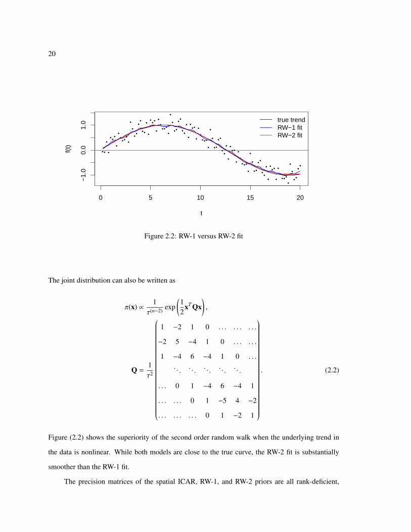
Figure (2.2) shows the superiority of the second order random walk when the underlying trend in
the data is nonlinear. While both models are close to the true curve, the RW-2 fit is substantially
smoother than the RW-1 fit.
The precision matrices of the spatial ICAR, RW-1, and RW-2 priors are all rank-deficient,

21
meaning the distribution of x is a singular multivariate normal distribution. Recall that the precision
matrix of the binary specification of the spatial ICAR and RW-1 is proportional to Dω −W, where
Dω is a diagonal matrix of the neighborhood sizes and W is the adjacency matrix. Each row and
column of Dω −W and of Q as defined in (2.2) sums to 0. Thus, the overall level of the vector x is
not identified because we can add a constant to x and get the same density:
π(x + c1) ∝ exp(12
(x + c1)T Q(x + c1))
= exp(12
xT Qx + 2c1T Qx + c21T Q1)
= exp(12
xT Qx).
Further, Qs = 0 for s = {1, 2, . . . , n}T for the RW-2 precision, which means the density is constant
when adding a linear trend to x. In practice the rank deficiency is accommodated by adding con-
straints to the vector x and adding an intercept to the model. The most common are 1T x = 0 when
Q is rank n − 1 with the addition of sT x = 0 when Q is rank n − 2.
2.3 Computation for Bayesian Models
Suppose y is a sample from a family of distributions indexed by some parameters θ. In the simplest
Bayesian models, we incorporate uncertainty in the parameters θ through a prior distribution that
may depend on some fixed hyper parameters γ. That is
y ∼ Pr(y | θ),
θ ∼ π(θ | γ).
Generally the goal of modeling is to estimate some functions of the posterior distribution of θ and
the variability of these estimates. Often we are interested in integrals of the form
Eθ|yg(θ) =
∫θ
g(θ)π(θ | y,γ)dθ. (2.3)

22
For some choices of the prior π(θ | γ), the posterior distribution, π(θ | y,γ), belongs to a known
family of distributions or is simple enough that we can get posterior estimates using basic analytic
approximation, Monte Carlo methods, or numerical integration. However, in many cases, Monte
Carlo methods such as direct sampling or importance sampling are difficult. In this section we de-
scribe two computational approaches for approximating integrals like (2.3). First we review the
Metropolis-Hastings algorithm, which is a widely applicable Markov chain Monte Carlo (MCMC)
sampler. Then we review integrated nested Laplace approximations (INLA), which is a tool specif-
ically developed for Bayesian hierarchical models that use Gaussian random effects. We use both
procedures throughout this thesis.
2.3.1 Metropolis-Hastings
The basic principle of MCMC is to construct a homogenous Markov chain with stationary distri-
bution equal to the target distribution, in our case the posterior distribution, and calculate the usual
sample statistics (means, variances, quantiles) from these chains to estimate important features of
the target distribution. The usefulness of this method hinges on a central limit theorem for Markov
chains known as the ergodic theorem. For integrable functions g(x), the ergodic theorem states
that if x = {x1, x2, . . . , xN} form an irreducible and positive recurrent Markov chain with stationary
distribution π, then [Bremaud, 1999, Flegal and Jones, 2011]
limN→∞
1N
N∑i=1
g(xi)→p Eπg(x).
Irreducibility means that the chain can get from any part of the state space to any other part of the
state space in a finite number of steps. If the state space of x is countable, then positive recurrence
means that if the chain starts in state i, the expected number of steps before returning to state i
is finite [Bremaud, 1999]. In general state spaces, the positive recurrence criteria is replaced with
Harris recurrence [Flegal and Jones, 2011].
The Metropolis-Hastings algorithm is a way to construct an ergodic Markov chain under very
general conditions on the stationary distribution π. The algorithm was first used by Metropolis

23
et al. [1953] and then conceived of more generally by Hastings [1970]. The Metropolis-Hastings
algorithm is a kind of accept-reject algorithm. Starting at a particular value xt, a candidate for the
next state, x′ is drawn from a proposal distribution q. The acceptance probability of this move is
constructed so that the stationary distribution of the entire chain is the target distribution.
The Metropolis-Hastings algorithm for constructing a sequence θ1, θ2, . . . , θN with stationary
distribution π(θ | y,γ) is
• Draw θ′ ∼ q(θ′ | θt).
• Calculate the acceptance ratio Rθ:
Rθ =π(θ′ | y,γ)q(θt | θ
′)π(θt | y,γ)q(θ′ | θt)
.
• Set θt+1 = θ′ with probability α = min{1,Rθ}.
The choice of proposal q is flexible. In some cases, it is possible to choose q to be symmetric,
meaning q(θ′ | θ) = q(θ | θ′). For example, if θ is real-valued, then a Gaussian random walk,
θ′ ∼ N(θ, σ2), is a symmetric proposal. Further, if θ is a vector, the proposal q may leave some parts
of θ unchanged. Updating small subsets (or blocks) of θ is common practice when the size of θ is
large or when there is high posterior correlation between some elements of θ.
The Metropolis-Hastings algorithm naturally accommodates posterior distributions that are known
only up to a proportionality constant. The acceptance ratio is often written with the product of the
likelihood and the prior
p(y | θ′)π(θ′ | γ)q(θt | θ)p(y | θt)π(θt | γ)q(θ′ | θt)
.
The main drawback of the Metropolis-Hastings sampler is that the proposal q much be chosen care-
fully to avoid poor convergence. Choices such as the Gaussian random walk may be inefficient, es-
pecially if the elements of θ are highly correlated in the posterior. Unfortunately, spatial or temporal
random effects are often highly correlated. Even with good proposals, the Metropolis-Hastings algo-
rithm can be slow if calculating the likelihood is computationally intensive (e.g., involves inversion

24
or multiplication or large matrices). Thus, more sophisticated MCMC methods or approximation
methods are sometimes preferred over simple Metropolis-Hastings sampling schemes.
2.3.2 Integrated Nested Laplace Approximations
One such approximation method is integrated nested Laplace approximation, or INLA. Developed
by Rue et al. [2009], the INLA approach is specific to Bayesian hierarchical models where the
latent variables are Gaussian. Let x be the latent variables (e.g., random effects), θ = {θ1, θ2} be the
parameters in the likelihood of y and prior on x, and γ be parameters for the priors on θ:
p(y | x, θ) =
n∏i=1
p(yi | xi, θ1),
x | θ2 ∼ N(µ(θ2),Q(θ2)−1
),
θ | γ ∼ π(θ | γ).
In our applications x will be a mean-zero GMRF, so µ(θ2) = 0. Then the full posterior for {θ, x} up
to a proportionality constant is
π(θ, x | y,γ) ∝ π(θ | γ)|Q(θ2)|1/2 exp
−12
xT Q(θ2)x +
n∑i=1
log (p(yi | xi, θ1))
. (2.4)
The basic approach of INLA is to approximate the marginal posterior distributions using a com-
bination of numerical integration and Gaussian approximation. Let π(· | ·) denote an approximate
conditional distribution. Then the approximate marginal posterior distributions are produced as
π(xi | y) =
∫θπ(xi | θ, y)π(θ | y)dθ
π(θ j | y) =
∫θ− j
π(θ | y)dθ− j.
Most of the approximations follow from a Gaussian approximation of π(x | y), which is equiva-
lent to finding a Gaussian approximation to the likelihood term,∑n
i=1 log (p(yi | xi, θ1)), in equation
(2.4). The approximation methods and integration techniques are discussed in detail in Rue et al.
25
[2009].
While INLA is powerful tool for Bayesian computation with latent GMRFs, the approach is
somewhat limited. While both INLA and MCMC can produce estimates of the marginal poste-
riors, MCMC approximates the full posterior, which is useful for estimating posterior correlation
or posterior predictive distributions. Thus, questions of posterior correlations between parameters
or of complex functions of the parameters can be difficult to address with INLA. Further, there is
a practical maximum of around 12 on the dimension of θ because the numerical integration step
for each π(θ j | y) is exponential in the size of θ [Rue et al., 2009]. Finally, INLA is not accu-
rate for all applications. For example, Fong et al. [2010] found that INLA was less accurate for
binomial data when the number of trials was small. Nonetheless, INLA is popular estimation tool
for spatial and temporal problems. An implementation of INLA is available as an R package from
http://www.r-inla.org/.

26
Chapter 3
TEMPORAL MODELS FOR CANCER INCIDENCE IN WASHINGTON STATE
3.1 Introduction
Time plays an important role in the incidence and progression of most diseases. However, there
is no “one size fits all” version of time that is appropriate for all types of health outcomes. While
seasonal factors are strong predictors of the risk of contracting illnesses like the flu, they are of
little relevance for cancer incidence. In arguing for the careful consideration of the appropriate time
scales for health data, Berzuini and Clayton [1994] state that time “is simply the scale along which
other causes operate” and that the role of time in statistical models is to act as a “surrogate or proxy
measure” for these unobserved processes that contribute to disease risk. Thus, it is important to have
a basic understanding of the dynamics of the disease endpoint when choosing how to incorporate
time into a model for disease risk.
In this chapter, we describe temporal models for cancer incidence for two common cancers:
female breast cancer and male lung cancer. Cancer is a collection of many different diseases and
illnesses that share the feature of unrestricted cell growth due to genetic changes that allow can-
cer cells to bypass or circumvent the body’s normal growth regulation mechanisms [Escedy and
Hunter, 2008]. There are two distinct processes to consider when the primary outcome of interest is
the number of incident cancer cases (i.e., the number of people being diagnosed with cancer). The
first is the process by which the genetic changes or mutations occur, and the second is the process
by which the cancerous cells are identified and the diagnosis of cancer is conferred. We account for
these processes on three time scales: age, year of diagnosis (period), and year of birth (cohort).
We use temporal models on these three time scales for prediction and inference. One of the main
purposes of fitting temporal models for disease incidence and mortality is to provide forecasts for
the number of cases or deaths. For example, every January, the American Cancer Society and Na-
27
tional Cancer Institute produce national and state-level forecasts for cancer mortality for the current
year and for the next 3 years [Ghosh and Tiwari, 2007, Zhu et al., 2012, 2013]. These projections
are then used for planning tasks such as estimating the total cost of cancer in the United States.
While the focus of this chapter is on time series data, we present models with the intention of ul-
timately extending these methods to include a spatial component and space-time interactions. There
are several classes of time series models that have been extended to spatiotemporal models. Gaus-
sian processes (GPs) are the dominant tool used for spatially continuous data rather than areal data,
and they are often used for stationary time series data. Spatial or temporal GPs have been extended
to model continuous spatiotemporal processes with either separable or non separable space-time
covariance functions [Gneiting and Guttorp, 2010]. Recently Quick et al. [2013] used a GP for time
together with an areal model for space to analyze monthly rates of hospital admissions for asthma
measured at the county level. However, they use a Gaussian likelihood that is less appropriate for
rare disease such as cancer because the rates are near zero. Diggle et al. [2005, 2013] use a spa-
tiotemproal GP as the basis of a spatiotemporal log Gaussian Cox process (LGCP). In an LGCP,
areal and discrete-time observations are based on aggregating a spatially and temporally continuous
Poisson point process with a log intensity surface that is a GP. However, our data are only available
at a fairly coarse level of aggregation in space and time (counties and years); whereas, the LGCP is
more appropriate when the locations of cases are available for smaller units such as UK postcodes
(which contain an average of about 20 households) and days.
Dynamic linear models (DLMs) or state space models have been a popular choice for Bayesian
time series and forecasting data for several decades [West and Harrison, 1997, Prado and West,
2010]. DLMs have been used in several applications for forecasting counts of disease cases and
deaths, including cancer mortality [Nobre et al., 2001, Ghosh et al., 2007], and more recently, there
has been increased attention in extending DLMs to handle multivariate time series data including
spatial time series data [Carvalho and West, 2007, Wang and West, 2009, Gamerman, 2010]. For
computational reasons, most applications involving DLMs assume a Gaussian likelihood, which
again may not be appropriate for rare diseases. An exception is the recent work of Windle et al.

28
[2014] who use a data augmentation scheme to form a Gibbs sampler for dynamic models with
binomial likelihoods.
In this chapter, we rely on a third approach based on Gaussian Markov random fields (GM-
RFs). Knorr-Held [2000] presents a framework that includes additive spatial and temporal random
effects with GMRF priors as well as for space-time interaction terms that are also Gaussian with
four possible covariance forms representing different kinds of separable and non separable interac-
tion. Models based on these space-time interaction priors can be estimated with integrated nested
Laplace approximation (INLA), so there are fewer computational barriers to using a non Gaussian
likelihood. Finally, the approach we take models change in disease risk along multiple time scales,
which is easily accommodated within the GMRF framework. In the first part of this chapter, we
introduce a framework for choosing which time scales are most informative for each cancer and for
generating forecasts from these models. In the second part of the chapter, we include covariates in
the temporal model using survey data on cancer screening and tobacco use.
3.2 Temporal Models for Cancer Incidence
In general, the risk of cancer increases with age. There are a few exceptions such as certain
leukemias and central nervous system tumors that are more common in children, but the two cancers
considered in this chapter adhere to the general rule of increasing risk with age. Age is a surrogate
for internal processes such as hormone exposure or the cumulative damage of random genetic mu-
tations when DNA is being copied, but it can also be a proxy for external factors such as cumulative
exposure to carcinogens. The period and cohort effects are both surrogates for exposure to external
factors. Period effects include environmental and diagnostic factors. For example, the introduction
of a new diagnostic procedure may lead to a jump in disease incidence across all age groups. Cohort
effects capture longer term causes of cancer that have changed over time. For example, inhalation
of asbestos is the primary cause of a lung cancer called mesothelioma. Earlier birth cohorts have
greater risk of mesothelioma than more recent cohorts because asbestos usage has decreased over
time [Miranda et al., 2014]. Generally, life style factors such as alcohol and tobacco use or diet are
also cohort effects because they have a delayed effect on cancer and changes in these factors differ

29
by age groups.
3.2.1 Age Period Cohort Models
The age-period-cohort (APC) model is an additive model for the log rate of incidence or mortality.
Let Y = {yi j : i = 1, . . . , A; j = 1, . . . ,T } be a matrix of counts in each of A age groups and T time
points. The cohort index k is a function of age and period. If the age scale and time scale are the
same (i.e., 5 year age bands and 5 year time intervals), then k = A− i+ j [Miranda et al., 2014]. If the
age intervals are M times longer than the time intervals, then the cohort index is k = M · (A − i) + j
[Heuer, 1997, Knorr-Held and Rainer, 2001]. The cohorts index the diagonals of the age-period
matrix, as shown for a small example in Table 3.1. Let N = {Ni j, i = 1, . . . , A; j = 1, . . . ,T } be
Year IndexAge Index 1 2 3 4 5
1 5 6 7 8 92 4 5 6 7 83 3 4 5 6 74 2 3 4 5 65 1 2 3 4 5
Table 3.1: Indices of the age, period, and cohort parameters for 5 equal-width age bands and timeintervals. The body of the table shows the cohort index for each age-year combination.
the size of the risk set for each age and time. For time intervals greater than one year, the entries
of N will be person-years. For single year time intervals, N is usually the population within each
age/period cell.
The basic APC model is [Clayton and Schifflers, 1987b]
log E[
yi j
Ni j
]= µi j = δ + αi + β j + γk. (3.1)
In this model, it is tempting to interpret δ as the overall log rate of incidence and to interpret dif-
ferences in the age effects, period effects, or cohort effects as log relative risks. However, direct
interpretation of these effects is difficult because the model is over parameterized.

30
If we stack the age, period, and cohort effects into a single vector, θ, then for a suitably defined
design matrix X, we have µ = δ + X′θ. The X in this case will be rank deficient because the entries
corresponding to the cohort effects are linearly depend on the entries for the age and period effects.
We discuss this issue in terms of identifiability and invariant forecasts in the next sections.
3.2.2 Identifiability of the age-period-cohort model
Several authors, beginning with Clayton and Schifflers [1987a,b], have discussed the non-identifiability
of the individual terms of the APC model. Kuang et al. [2008b] and Nielson and Nielsen [2014]
define the identifiability issue from a group theoretic perspective. The overall mean as given in (3.1)
is invariant to a translation on each set of effects and addition of a linear trend in the age, period, and
cohort parameters. For equal-width age and time intervals, we call this group of transformations G1
with members
g1 :
αi
β j
γk = γA−i+ j
δ
→
αi + a + (i − 1)d
β j + b − ( j − 1)d
γA−i+ j + c + (A − i + j − 1)d
δ − a − b − c + (A − 1)d
,
for any real numbers a, b, c, d. For 5 year age bands and 1 year time intervals, we call the group of
transformations G2 with members g2[Knorr-Held and Rainer, 2001]
g2 :
αi
β j
γk = γ5·(A−i)+ j
δ
→
αi + a + 5(i − A+1
2
)d
β j + b −(
j − T+12
)d
γ5·(A−i)+ j + c +(M · (A − i) + j − MA−M+T
2
)d
δ − a − b − c
.

31
The overall log rates are invariant with respect to these transformations. That is, for any g (in G1 or
G2 depending on the data), µi j(g(αi, β j, γk, δ)) = µi j(αi, β j, γk, δ). For example
µi j(g1(αi, β j, γk, δ)) = g1(αi) + g1(β j) + g1(γk) + g1(δ)
= αi + a + (i − 1)d + β j + b − ( j − 1)d + γA−i+ j + c
+ (A − i + j − 1)d + δ − a − b − c − (A − 1)d
= αi + β j + γA−i+ j + δ + a + b + c − a − b − c
+ (i − 1 − j + 1 + A − i + j − 1 − A + 1)d
= αi + β j + γA−i+ j + δ
= µi j(αi, β j, γk, δ).
Since the data likelihood only depends on the age, period, and cohort parameters through this overall
log rate, the likelihood of the observed data is also invariant to these groups of transformations.
Thus, the age, period, and cohort effects are not identifiable.
3.2.3 Invariant Forecasts with the APC model
In many applications, forecasts of mortality or incidence rates are important. Given the identifiabil-
ity issues, it is crucial to choose forecasts that are invariant to the group of transformations. Suppose
we forecasts rates h years ahead in time for the same set of age groups. Then we want
µi,T+h = δ + αi + βT+h + γk+h,
where k = A − i + T or k = M(A − i) + T . The forecasts depend on projecting the period and cohort
effects ahead h steps based on the fitted period and cohort effects for the observed data. That is, for
some function fβ and fγ,
βT+h = fβ(β1:T ) and γk+h = fγ(γ1:k).

32
If h < A, then we project at most h new cohort effects because the rest are estimated with the
observed data. For example, Table 3.2 shows that to predict 3 years ahead for the small example
in Table 3.1, we need to forecast the period effect for time j = 8 and the cohort effects for k =
10, 11, 12.
1 2 3 4 5 6 7 81 5 6 7 8 9 10 11 122 4 5 6 7 8 9 10 113 3 4 5 6 7 8 9 104 2 3 4 5 6 7 8 95 1 2 3 4 5 6 7 8
Table 3.2: Indices of the age, period, and cohort parameters for equal-width age bands and timeintervals. The body of the table shows the cohort index for each age-year combination. The boldedindices indicate the period and cohort effects that need need to be forecasted to generate predictionsfor time periods 6-8.
The projected log rates {µi,T+h, i = 1, . . . , A} are not invariant to the group of transformations for
all choices of fβ and fγ. Instead, the projection functions must satisfy
g( fβ(β1:T )) = fβ(g(β1:T )) and g( fγ(γ1:T )) = fβ(g(γ1:T )).
Kuang et al. [2008a] outline several choices for fβ and fγ that adhere to these constraints. One of
their suggestions is to project linearly from the most recent effect using the average first differences
between effects. For example, the projection for period effects is
fβ(β1:T ) = βT + hsβ (3.2)
where sβ =1
T − 1
T∑j=2
∆β j.

33
Applying this projection to the group transformed period effects yields
fβ(g1(β1:T ) = βT + b − (T − 1)d +h
T − 1
T∑j=2
(∆β j − d( j − 1 − j + 2)
)= βT +
hT − 1
T∑j=2
∆β j + b − d(T + h − 1)
= βT + hsβ + b − (T + h − 1)d
= g1( fβ(β1:T ))
This guarantees that µ(g(αi, βT+h, γk+h, δ)) = µ(αi, βT+h, γk+h, δ). The standard RW-1 projection
(constant at the last observed effect) does not give invariant projections of the log rate, but the RW-2
projection does:
βT+h | β1:T ∼ N
βT + h∆βT ,1 + 22 + · · · + h2
τ2β
,g1(βT ) + hg1(∆βT ) = βT + b − d(T − 1) + h
[βT + b − d(T − 1) − βT−1 − b + d(T − 2)
]βT + b − d(T − 1) + h
[βT − βT−1 − d
]= βT + h∆βT + b − d(T + h − 1)
= g1(βT + h∆βT ).
RW-2 projection is also a linear projection from the latest effect, but the slope is the last first differ-
ence rather than the average of the all the first differences. In practice we found that both methods
give similar projections for the number of cases (see appendix A).
3.3 A Bayesian APC Model
Most attempts at fitting the full APC model rely on arbitrary constraints to overcome the identi-
fiability issues described in the previous section. For example, Carstensen [2007] suggests fitting
smoothing splines to produce age, period, and cohort functions while imposing a set of constraints
for identifiability. These constraints include setting some age, period, or cohort effects to 0 for cho-
34
sen reference groups and restricting the average slope of the smoothing splines.
However, the second differences of the age, period, and cohort effects are identifiable and in-
variant to the group of transformations defined above [Clayton and Schifflers, 1987b, Kuang et al.,
2008a]. That is ∆2αi(g(α)) = ∆2αi(α) :
∆2αi(g1(α)) = g1(αi) − 2g1(αi−1) + g1(αi−2)
= αi + a + (i − 1)d − 2αi−1 − 2a − 2(i − 2)d + αi−2 + a + (i − 3)d
= αi − 2αi−1 + αi−2 + a − 2a + a + d(i − 2 − 2i + 4 + i − 3)
= ∆2αi(α).
The second differences can be interpreted as “accelerations” in the effects. They also define the
curvature of the age, period, and cohort profiles. On the rate scale, second differences are ratios of
relative risks. Thus, it is sensible to choose a modeling framework that deals directly with second
differences.
Several authors have suggested a Bayesian formulation of the APC model with the RW-1 or
RW-2 priors introduced in chapter 2 [Berzuini and Clayton, 1994, Besag et al., 1995, Knorr-Held
and Rainer, 2001, Riebler et al., 2012]. Recall that the RW-2 prior follows from assuming that the
second differences are independent, identically distributed Gaussian random variates. Further, the
usual implementation of the RW-2 prior (including the implementations in the INLA package and in
WingBUGS) incorporates sum-to-zero and zero slope restrictions to overcome the rank deficiency of
the RW-2 prior. Additional, unstructured random effects are included in the Bayesian APC models
to allow for heterogeneity around the constrained temporal effects.
The full specification of this Bayesian APC model is
yi j ∼Poi(Ni j exp(µi j))
µi j =δ + αi + β j + γk + zi j,
δ ∼ N(0, σ2δ),
35
α ∼ RW-2(τ2α), τ2
α ∼ Ga(a1, b1),
β ∼ RW-2(τ2β), τ
2β ∼ Ga(a1, b1),
γ ∼ RW-2(τ2γ), τ2
γ ∼ Ga(a1, b1),
z ∼ N(0, τ−2z I), τ2
z ∼ Ga(a2, b2).
In this model, we use the same prior for the precisions on each set of RW-2 random effects and a
different prior on the precision of the independent random effects. Initially we follow the suggestion
of Knorr-Held and Rainer [2001] and use (a1, b1) = (1, 0.00005) and (a2, b2) = (1, 0.005). Using the
same prior all RW-2 effects is not necessarily intuitive. For the breast cancer and lung cancer data,
there are A = 13 age groups and nearly 80 cohorts. A priori, we expect the age effects to be larger
and changing more quickly than the cohort effects, which means we expect that the precision of the
age effects will be much smaller than the precision of the cohort effects. In principle, this suggests
we should specify different priors for τ2α and τ2
γ. However the suggested priors are sufficiently non
informative that, in practice, we can get different estimates for the precisions of the age, period, and
cohort effects.
We fit models to breast and lung cancer incidence data from the Washington State Cancer Reg-
istry using the Bayesian APC model and the Carstensen model. In both cases, the data are 13 × 19
matrices, where 13 is the number of age bands (25 − 29, 30 − 24, . . . 80 − 84, 85+) and 19 is the
number of years (1992–2010). We restrict to cases of breast cancer among women and lung cancer
among men. We summarize the total incidence by age and year in Tables 3.3 and 3.4. For breast
cancer, there are no counts under 15 and only 11 age-year combinations with fewer than 25 counts.
In contrast, lung cancer is rare for the youngest age bands included here. There are 5 age-year com-
binations with zero cases and 38 age-year combinations with at most 5 cases of lung cancer.
Figure 3.1 shows the estimated age, period, and cohort effects from the smoothing splines
model of Carstensen [2007] and the Bayesian APC model for breast cancer. We fit the Carstensen
model using the Epi package in R using natural splines with 5, 5, and 15 knots for the age, pe-
riod, and cohort functions, respectively. We fit the Bayesian APC model using integrated nested

36
Breast Lung(25,30] 432 20(30,35] 1449 66(35,40] 3720 225(40,45] 7735 537(45,50] 11310 1386(50,55] 12088 2321(55,60] 12186 3672(60,65] 11749 5334(65,70] 10808 6584(70,75] 10172 7063(75,80] 8612 6223(80,85] 6078 3879
(85,110] 4123 2151
Table 3.3: Total incidence by age band.
Laplace approximations with the INLA package. We transformed each set of effects using (possibly
different) transformations in G2 so that the age, period, and cohort effects of both models sum to
zero and so that the period effects have a slope of zero. The y-axis is purposefully missing a scale
because the individual effects are not identifiable. The age and period curves are similar for these
methods. Both age curves show an increase in the log incidence rate with age that levels off and
even decreases slightly in the oldest age groups.
The period curves show an increase to a peak around 2000, then a decrease followed by a pos-
sible increase. However the posterior median of the standard deviation of the period effects is one
tenth that of the age effect, suggesting that year-to-year variability in breast cancer rates is far less
substantial than age-to-age variability. The slight linearly increasing tend in the cohort effects of the
Bayesian model should not be over interpreted because it could just be an artifact of the transforma-
tion. Finally, the “wiggling” of the cohort effects in the Carstensen model depends on the number
of knots chosen for the natural splines.
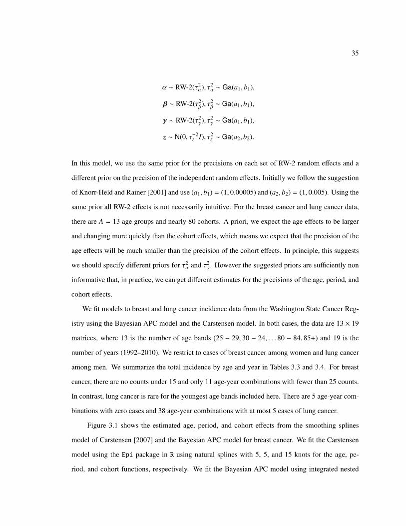
Figure 3.2 shows the estimated age, period, and cohort effects for lung cancer. The age and
cohort curves are similar for these methods. Both show an increasing trend in lung cancer incidence
and a decreasing trend in cohort (birth year). The age curve estimated by the Bayesian APC model

37
Age Effects (σα) = 0.188
Age
(25,30] (35,40] (45,50] (55,60] (65,70] (75,80] (85,110]
Carstensen, 2007Knorr−Held et al., 2001
Period Effects (σβ) = 0.016
Period
1992 1994 1996 1998 2000 2002 2004 2006 2008 2010
Cohort Effects (σβ) = 0.008
Cohort
1910 1920 1930 1940 1950 1960 1970 1980
Age, Period, and Period Curves for Breast Cancer
Figure 3.1: Fitted APC curves for breast cancer using the Bayesian APC model and the smoothingsplines model in [Carstensen, 2007] and the posterior median of the standard deviation of theseeffects in the Bayesian APC model. The y-axis is purposefully missing a scale because the individualeffects are not identifiable.

38
Breast Lung1992 3801 20321993 4052 19191994 4353 20001995 4456 19641996 4460 19961997 4970 20361998 5303 21421999 5476 21642000 5424 20452001 5630 20752002 5751 20902003 5506 21062004 5462 20912005 5635 21272006 5539 21342007 5592 19882008 6183 21092009 6625 22182010 6244 2225
Table 3.4: Total incidence by year.
levels off in the older age groups, but the Carstensen effects do not. These initial results suggest
that fitting the full APC model may be unnecessary for breast and lung cancer. For both cancers we
see clear “accelerations” in the incidence rates as age increases, and for lung cancer, we see clear
“deceleration” in the rates as the birth year increases. The relationships between the incidence rates
and the remaining effects are less clear. In the next section we propose a framework for choosing
which temporal scales are most informative for each cancer.
3.4 The APC Model for Breast Cancer and Lung Cancer
For each cancer, we fit four models: age (A), age-period (AP), age-cohort (AC), and age-period-
cohort (APC). The names of the models refer to which effects are included in the model. We show
the results for the best fitting model for each cancer. We choose the best fitting model based on three
39
Age Effects (σα) = 0.138
Age
(25,30] (35,40] (45,50] (55,60] (65,70] (75,80] (85,110]
Carstensen, 2007Knorr−Held et al., 2001
Period Effects (σβ) = 0.007
Period
1992 1994 1996 1998 2000 2002 2004 2006 2008 2010
Cohort Effects (σβ) = 0.211
Cohort
1910 1920 1930 1940 1950 1960 1970 1980
Age, Period, and Period Curves for Lung Cancer
Figure 3.2: Fitted APC curves for lung cancer using the Bayesian APC model and the smoothingsplines model in [Carstensen, 2007] and the posterior median of the standard deviation of theseeffects in the Bayesian APC model. The y-axis is purposefully missing a scale because the individualeffects are not identifiable.

40
criteria that capture within-sample fit, out-of-sample prediction, and complexity.
• CPO: the conditional predictive ordinant is a Bayesian analogue of leave-one-out cross val-
idation and is often used in model diagnostics to find points that are outliers with resect to a
particular model [Pettit, 1990, Held et al., 2010]. It is defined component-wise as
CPOi = π(yobsi j | y−i j)
=
∫π(yobs
i j | y−i j, θ)π(θ | y−i j)dθ.
We compare the four models based on the total log CPO, which is a measure of overall fit.
• MSE: we fit each model to the 1992–2007 data and then predict the 2010 counts using the
period and cohort forecasts defined in equation (3.2). We compare the four models based on
the average MSE for the predicted counts:
MSE =113
13∑i=1
Eθ,yi,2010 |y1992−2007
(yi,2010 − yobs
i,2010
)2.
• DIC: the deviance information criterion is a measure of goodness of fit penalized by model
complexity [Spiegelhalter et al., 2002]. DIC is the sum of the deviance at the posterior mean
of the parameters and a penalty 2pD. The deviance is
D(θ) = −2 log p (y | θ) + cy,
where cy depends only on the observed data. The penalty pD, often called the effective number
of parameters, is the difference of the posterior mean of the deviance and the deviance at the
posterior mean. Spiegelhalter et al. [2002] present DIC as a Bayesian version of AIC, which
is in turn an approximation to model selection via cross validation in the maximum likelihood
setting. However, Plummer [2008] shows that the approximation to cross validation breaks
down when the number of effective parameters is similar the number of observations, which
is usually the case for spatial models and the temporal models used in this chapter. In these

41
models, DIC tends to under penalize more complex models.
For these criteria, larger values of CPO are considered better and smaller values of MSE and DIC are
considered better. All three criteria are easy to compute using Markov chain Monte Carlo (MCMC),
and CPO and DIC are available from INLA. We rely on INLA except for the forecasting com-
parisons. We found that MCMC (implemented in WinBUGS) and INLA produce nearly identical
estimates for the overall log rates and the age, period, and cohort effects. There are some differences
in the estimates of the precisions, especially when they are large. See appendix A for a comparison
of MCMC and INLA for two of the models considered below.
We give all results for the specific choices of hyper parameters and constraints on the intrinsic
GMRFs given in section 3.3. While the results will change for difference settings of these hyper
parameters and constraints, we expect that the conclusions for breast cancer and lung cancer will
robust to these choices because the models supported by these data are clear. A thorough sensitivity
analysis to both the hyper parameters and the restriction on the GMRF priors should be carried out
if there is less clarity in the appropriate models.
3.4.1 Breast Cancer
First we fit models to the breast cancer incidence data. The bottom panel in Figure 3.3 shows the ob-
served log rates for the 13 age groups over 19 years. The rates are flat in time, though there is slight
decreasing trend starting in 2003. The effect of age is most prominent. There are large increases in
risk for the youngest four age groups and then similar rates for the oldest groups. The parallel lines
suggest that there are no strong cohort effects.
The model fit statistics and estimated components confirm these observation. The AP model
is the best on all three metrics (see Table 3.5). The full APC model also does well on the metrics
computed with the full data but lacks on the mean squared error of the forecasts for the 2010 counts.
Figure A.3 in appendix A shows the posterior mean for the predicted 2010 counts versus the ob-
served counts for all for models. All four models do well for the smaller counts (which correspond
to the youngest age groups), but the predictions from the AP model are the closest to the observed

42
counts for larger counts. Thus, we prefer the simpler AP model to the full APC model for prediction.
The top panel in Figure 3.3 shows the fitted log rates from the AP model, and the middle panel
CPO MSE DICA 2.823 5476 2285.53
AP 3.046 3347 2277.46AC 2.811 8528 2287.74
APC 3.041 4313 2277.63
Table 3.5: Comparison of models for breast cancer incidence rates. The models are age (A), age-period (AP), age-cohort (AC), and age-period-cohort (APC). The comparison criteria are the con-ditional predictive ordinant (CPO), the mean squared error in forecasts of the 2010 counts based ondata up to 2007 (MSE), and the deviance information criterion (DIC).
A AP AC APCδ -6.105 -6.106 -6.103 -6.104
σα 0.186 0.187 0.184 0.188σβ – 0.016 – 0.016σγ – – 0.004 0.008σz 0.073 0.070 0.089 0.070
Table 3.6: Posterior medians for the overall log rate and variance components for breast cancer.
shows the fitted log rates versus the observed log rates. For the older age groups, the fitted log rates
are very similar to the observed log rates. For the younger age groups, the model smooths most of
the year-to-year variability in the observed incidence rates. The middle panel shows that the fitted
rates for the first two age bands have been substantially smoothed to essentially the same value over
all 19 years. By the third age group, (35, 40], the observed rates are much less volatile, and the fitted
rates show less smoothing.
Table 3.6 shows posterior estimates of the standard deviations of the random effects and the
overall log rate. The posterior median of exp(δ) is consistently estimated at approximately 223 peo-
ple per 100, 000 individuals across the four models. The standard deviations for the age and period
random effects are also fairly constant, indicating that the magnitude of the age and period effects

43
does not change when adding in the cohort effects. Further, the standard deviation of the unstruc-
tured random effects does increase when the period effects are excluded in the AC and A models.
While age explains the bulk of the heterogeneity in the rates, there is some temporal structure in the
rates in addition to the age structure.
3.4.2 Lung Cancer
Now we turn our attention to the lung cancer incidence data. The bottom panel in Figure 3.4 shows
the observed log rates for lung cancer incidence among men. The curve for the youngest age group
is incomplete because there several are years with no incident cases. Again we see a large age effect
with large jumps in the log incidence rate in the first seven age bands and then more homogeneity
in the incidence rate for the older age groups. In contrast to the breast cancer rates, the lung curves
are not parallel. While the age curves for some age groups are flat, in other age groups (such as
the (55 − 60] group), the incidence rates are decreasing. This suggests that there are non-negligible
cohort effects for lung cancer incidence. The AC and APC models clearly out perform the A and
AP models in terms of within sample fit (see Table 3.7). Again, the more complex APC model
lacks on the mean squared error of the 2010 forecasts, especially for larger counts (see Figure A.3
in appendix A).
The top panel in Figure 3.4 shows the fitted log rate curves for the AC model with clear
CPO MSE DICA 12.65 6081 1884.03
AP 13.68 1726 1852.95AC 15.06 396.6 1768.45
APC 15.05 546.4 1768.37
Table 3.7: Comparison of models for lung cancer incidence rates. The models are age (A), age-period (AP), age-cohort (AC), and age-period-cohort (APC). The comparison criteria are the con-ditional predictive ordinant (CPO), the mean squared error in forecasts of the 2010 counts based ondata up to 2007 (MSE), and the deviance information criterion (DIC).
decreasing trends in incidence for the younger age groups. We investigate cigarette smoking rates

44
Fitted Log Rates−−Breast Cancer
year
log
inci
denc
e ra
te
1992 1993 1994 1995 1996 1997 1998 1999 2000 2001 2002 2003 2004 2005 2006 2007 2008 2009 2010
−9
−8
−7
−6
−5
(25,30] (30,35] (35,40] (40,45] (45,50] (50,55](55,60] (60,65] (65,70] (70,75] (75,80] (80,85] (85,110]
●
●
●
●●
●
●●
● ●●●
●
●
●
●
●
●●
●
●●●●
●
●
●
●
●
●
●
●
●●
●●●
●
●
●
●
●
●
●
●
●
●●
●●●
●
●
●
●
●
●
●
●●
● ●●
●
●
●
●
●
●
●●
●
●●●
● ●
●
●
●
●
●
●
●
●●
●●●
●
●
●
●
●
●
●●
●●
●●
●●
●
●
●
●
●
●●
●
●●●●
●
●
●
●
●
●
● ●
●●
●● ●●
●
●
●
●
●
●●
●
●● ●●
●
●
●
●
●
●
●●
●
●●
●●
●
●
●
●
●
●
●●●
●●● ●
●
●
●
●
●
●
●●
●●
●●●
●
●
●
●
●
●
●●
●
●●●●●
●
●
●
●
●
●●●
●● ●●
●
●
●
●
●
●
●●●
●●
●●
●
●
●
●
●
●
●●●
●●
●●●
●
●
●
●
●
●●
●
●●
●●●
●
−9 −8 −7 −6 −5
−9
−8
−7
−6
−5
Raw Log Rates
Fitt
ed L
og R
ates
Raw Log Rates−−Breast Cancer
year
log
inci
denc
e ra
te
1992 1993 1994 1995 1996 1997 1998 1999 2000 2001 2002 2003 2004 2005 2006 2007 2008 2009 2010
−9
−8
−7
−6
−5
(25,30] (30,35] (35,40] (40,45] (45,50] (50,55](55,60] (60,65] (65,70] (70,75] (75,80] (80,85] (85,110]
Figure 3.3: Fitted versus observed log rates for breast cancer. The fitted rates are based on theage-period model.

45
A AP AC APCδ -7.479 -7.477 -7.543 -7.542
σα 0.164 0.166 0.137 0.138σβ – 0.006 – 0.007σγ – – 0.008 0.211σz 0.152 0.104 0.038 0.037
Table 3.8: Posterior medians for the overall log rate and variance components for lung cancer.
as one possible explanation of these cohort effects in the next section. The middle panel shows the
fitted log rates versus the observed log rates. The fit is less tight around the observed rates than with
breast cancer, especially when the log rate is less than −8. This is consistent with our intuition that
there is more volatility in the observed rates and hence more smoothing with rare outcomes.
Table 3.8 shows posterior estimates of the standard deviations of the random effects and the
overall log rate. The estimates for the rate of lung cancer differ slightly depending on whether
the cohort effects are included. For the A and AP models, the estimate of exp(δ) is approximately
56 cases per 100, 000 individuals and, for the AC and APC models, approximately 53 cases per
100, 000. The standard deviations for the age effects and the unstructured random effects decrease
when the cohort effects are included, suggesting that there is a cohort structure in lung cancer rates.
3.5 Incorporating Covariates in the APC model
In this section, we describe how to incorporate covariates in the Bayesian APC model. For breast
cancer, we include screening through mammography as a possible explanation for age and period
effects, and for lung cancer, we include cigarette usage as a possible explanation for cohort ef-
fects. The screening and smoking data come from the Behavioral Risk Factor Surveillance System
(BRFSS). Although the BRFSS data and the cancer incidence data are both available as individual
records, we do not have joint screening/smoking and cancer information on the individual level.
This poses three challenges. First we must choose a sensible aggregate model to estimate the actual
effect of exposure rather than an ecological effect. Second, the BRFSS survey is not a simple ran-

46
Fitted Log Rates−−Lung Cancer
year
log
inci
denc
e ra
te
1992 1993 1994 1995 1996 1997 1998 1999 2000 2001 2002 2003 2004 2005 2006 2007 2008 2009 2010
−13
−11
−9
−7
−5
(25,30] (30,35] (35,40] (40,45] (45,50] (50,55](55,60] (60,65] (65,70] (70,75] (75,80] (80,85] (85,110]
●
●
●
●
●
●
●
●●
●●●●
●
●
●
●
●
●
●
●
●● ●●
●
●
●
●
●
●
●
●
●
●●●●
●
●
●
●
●
●
●
●
●
●● ●
●●
●
●
●
●
●
●
●
●
●●●●
●
●
●
●
●
●
●
●
●
●●●●
●
●
●
●
●
●
●
●
●
●● ●●
●
●
●
●
●
●
●
●
●●● ●
●
●
●
●
●
●
●
●
●● ●●
●
●
●
●
●
●
●
●
●
●● ●●
●
●
●
●
●
●
●
●
●
●●●
●
●
●
●
●
●
●
●
●
●
●●●
●
●
●
●
●
●
●
●
●
●
●●●
●
●
●
●
●
●
●
●
●
●●●
●
●
●
●
●
●
●
●
●
●
●●●●
●
●
●
●
●
●
●
●
●●●
●
●
●
●
●
●
●
●
●
●
●●●
●
●
●
●
●
●
●
●
●
●
●● ●
●
●
●
●
●
●
●
●
●
●
●● ●
●
−12 −10 −8 −6
−12
−10
−8
−6
Raw Log Rates
Fitt
ed L
og R
ates
Raw Log Rates−−Lung Cancer
year
log
inci
denc
e ra
te
1992 1993 1994 1995 1996 1997 1998 1999 2000 2001 2002 2003 2004 2005 2006 2007 2008 2009 2010
−13
−11
−9
−7
−5
(25,30] (30,35] (35,40] (40,45] (45,50] (50,55](55,60] (60,65] (65,70] (70,75] (75,80] (80,85] (85,110]
Figure 3.4: Fitted versus observed log rates for lung cancer. The fitted rates are based on the age-cohort model.

47
dom sample, so aggregate exposure summaries must take into account the survey design. Finally,
the women’s health module of the BRFSS survey is only included in even years after 2000, so we
must interpolate the mammography rates for five missing years.
3.5.1 Aggregate Regression Model
For a binary exposure, it is straightforward to derive the aggregate mean model by starting with
the individual model [Wakefield, 2007]. Suppose the probability of disease for an individual l is
exp(αi(l) + β j(l) + γk(l)) exp(λ0 + λ1zl), where zl is an indicator of whether person l is exposed. Here
we have left off the overall log rate δ from the APC model because it is redundant with exp(λ0) in
the model. The mean for the aggregate count within a particular age group and time period is
Eyi j =
Ni j∑l=1
exp(αi + β j + γk) exp(λ0 + λ1zl)
= exp(αi + β j + γk)Ni j∑l=1
exp(λ0 + λ1zl)
= exp(αi + β j + γk)[Ni j(1 − xi j) exp(λ0) + Ni jxi j exp(λ0 + λ1)
]= Ni j exp(αi + β j + γk)
[(1 − xi j) exp(λ0) + xi j exp(λ0 + λ1)
]where xi j =
∑Ni j
l=1 zl/Ni j is the proportion exposed in age group i during time period j. This is not
the same model as simply augmenting the APC model with a regression term
Eyi j = Ni j exp(αi + β j + γk + δ + λ′1xi j).
In this case, the coefficient λ′1 is an ecological effect rather than an individual level effect. In this
ecological model, we implicitly assume the exposure has a contextual effect, meaning that disease
risk is associated average exposure within the groups of aggregation rather than individual risk
[Wakefield and Lyons, 2010]. Knorr-Held and Rainer [2001] use an ecological APC model for lung
cancer data by including a lagged estimate of tobacco sales. To the best of our knowledge, the
aggregate mean model has not been used with APC models.

48
The appropriate aggregate mean model is no longer in the form of the usual link function as
introduced in section 1.2. Instead we have defined a two-parameter link function
h(θ1, θ2) = exp(θ1) · θ2.
Because the Gaussian random effects will only appear in one part of link function (in this case θ1),
this model still fits within the class of posteriors that can be approximated with integrated nested
Laplace approximation (see equation (2.4) in section 2.3.2). However, this link function is not
currently available in the INLA package for R, so we fit this model using MCMC (with WinBUGS).
3.5.2 Estimating Exposure from Survey Data
In general, we do not have access to the exposure status for all individuals in the population, so we
estimate xi j based on survey data. BRFSS is a large phone based survey of health outcomes, atti-
tudes, and risk factors. This survey is not a simple random sample of all individuals within the study
area. Instead, phone numbers are selected with different probabilities depending on whether they
are likely to be residential phone numbers and on the county with which the number is associated
(based on the area code and prefix). The probability that an individual takes the survey also depends
on the number of adults sharing the telephone and on the number of telephones per household. We
use sampling weights (the reciprocal of the sampling probability) to account for the unequal selec-
tion probabilities resulting from the design of the BRFSS survey. The sampling weights are [WA
CHS, 2010]
sample weight = stratum weightnum adults
num phones.
The stratum weight accounts for the differential probabilities in calling particular area code/prefix
combinations. The number of adults per household and number of residential telephone number per
household are based on each individual’s response to the survey.
Given the sample weights, we can estimate the total number people exposed and the total pop-
ulation size within each group using the Horovitz-Thompson estimator [Horvitz and Thompson,

49
1952]. Let wl be the sample weight for the lth individual, and suppose ni j people are sampled within
age band i at time j. Then the estimated total number exposed is
Ti j =
ni j∑l=1
wlzl,
and the estimated total population size is
Ni j =
ni j∑l=1
wl.
The survey weight can be interpreted as the number of people in the population represented by
the sampled individual. That is, a person sampled with probability π represents 1/π people in the
population, and Ni j = Ni j [Lumley, 2011]. In general each sampled person does not represent 1/π
people in the population because of issues such as non response. We correct for this by adjusting
the survey weights using poststratification. Suppose, for example, that Ntc is the total population
of county c at time t. We adjust the sample weights so that the weights for respondents from each
county add up to the total population of the county. That is, the weights for an individual in county
c are now
w′l = wlNtc∑A
i=1 Nitc.
Figure 3.5 shows the estimated smoking rates among men in Washington State using the post-
stratified weights. Individuals are defined as “smokers” if they reported smoking at least 100
cigarettes. This could include individuals that no longer smoke or who are not regular smokers.
Unlike the cancer rates, there is no clear trend in smoking rates by age group. In fact, the oldest
age group (85+) has the lowest estimated smoking rates, which may be because there is an inherent
selection bias towards non smokers in the BRFSS design (i.e., smokers may have health issues that
resulted in death before age 85 or being placed in a long term care facility without a direct phone
number). The average change in smoking rates from 1992 to 2009 is −4.4 percentage points; how-
ever, there are some age groups that show an increase in smoking rate over time. For example, the
smoking rate for the 75–80 group increases by 20 percentage points. Such a large increase in the
50
Year
Sm
okin
g R
ate
1992 1994 1996 1998 2000 2002 2004 2006 2008 2010
0.1
0.3
0.5
0.7
25−29 30−34 35−39 40−44 45−49 50−5455−59 60−64 65−69 70−74 75−79 80−84 85+
Figure 3.5: Estimated smoking rates among males in Washington State by age and year. They arethe estimated proportions of men who have smoked at least 100 cigarettes.
estimated smoking rate is likely to be a result of a much smaller increasing trend coupled with large
sampling variability in the estimates of smoking rates in earlier years when the BRFSS sample size
is much smaller.
3.5.3 Smoothing and Interpolation of Exposure Rates
In this section we propose a way to estimate rates for missing years. This same method can be used
to produce more reliable exposure rates when the sample sizes used to produce initial estimates are
small. We base our interpolation and smoothing scheme on the spatial smoothing model of Mercer
et al. [2013]. These authors investigate different methods for producing prevalence estimates at the
zip code level for the 2006 BRFSS data. One approach that these authors discuss is to transform
the initial estimated rates using the logistic transformation and to model the transformed rates as
Gaussian. Let xi j be the estimates using the poststratification method described in section 3.5.2 and

51
let xLi j be the logistic transform of these rates:
xLi j = log
[xi j/(1 − xi j)
].
Then the asymptotic distribution of these logistic transformed rates is
xLi j ∼ N
log[
pi j
1 − pi j
],
var(xi j)
x2i j(1 − xi j)2
,where pi j is the true rate for age group i at time j. The variance of the original estimates, var(xi j),
depends on the weights. We calculate this variance using the poststratification tools in the survey
package in R.
Mercer et al. [2013] use Gaussian Markov random fields to smooth estimates on the transformed
scale. Because their application is spatial, they use the convolution model with intrinsic CAR and
unstructured random effects [Besag et al., 1991]. In place of the convolution prior, we use a modified
age-period model with RW-2 priors on the age and year effects and additional heterogeneity by year:
E(xLi j) = µ + αi + β j + b j,
where π(α) and π(β) are RW-2 priors and π(µ) and π(b) are independent normal priors. We then
transform the posterior median for each age-year combination to produce smoothed exposure rates.
We can use the smoothed rates just for imputation in years without data, or we can use this
framework to both impute and smooth some or all of the initial rate estimates. Figure 3.6 shows
the mammography rates by age and year using the model only to impute missing years and using
all the smoothed estimates. Here the rate is the estimate of the proportion of women who have had
a mammogram in the last year. The middle panels shows the smoothed rates versus the original
estimates for those years in which data are available. In many cases, there is little difference in the
original and the smoothed estimates. In a few cases, there is significant smoothing. For example,
the mammography rates in the 85+ age group are very volatile in the first few years. For 1992 and

52
1993, these rates are based on samples of less than 15 women.
In the next section we consider three different version of the rates: the original and imputed
rates, the smoothed rates, and a hybrid approach in which the original rates are used except when
the sample size is less than 50. The cutoff of 50 is based on the CDC recommendation not to
interpret or report a percentage based on fewer than 50 respondents. In practice, this leads to using
the smoothed estimates for 1-2 age groups per year up to 2003 and then using only the original
estimates after 2003.
3.6 Results of the Aggregate Regression Models
We fit aggregate and ecological models to breast cancer and lung cancer using the best models
identified in section 3.4. For breast cancer, we fit age-period models
µaggi j = exp(αi + β j + zi j)
[(1 − xi j) exp(λ0) + xi j exp(λ0 + λ1)
],
µecoi j = exp(αi + β j + zi j + λ0 + xi jλ1).
For lung cancer, we fit age-cohort models
µaggi j = exp(αi + γk + zi j)
[(1 − xi j) exp(λ0) + xi j exp(λ0 + λ1)
],
µecoi j = exp(αi + γk + zi j + λ0 + xi jλ1).
In both cases, we use the original rates (including interpolated years for mammography rates), only
smoothed rates, and hybrid rates. Hybrid rates are the original poststratified estimates except when
the number of sampled individuals for an age-year combination is less than 50, in which case the
hybrid rate is the smoothed rate. The priors on the age, period, cohort, and unstructured random
effects are the same as in section 3.4. For the regression parameters, we use λ0, λ1 ∼ N(0, 100).
Tables 3.9 and 3.10 show the estimated effects and variance components for these models. We
include estimates from the ecological model only to stress that the effects estimated in ecological
models refer to different exposure measures and thus produce different estimates. For the breast
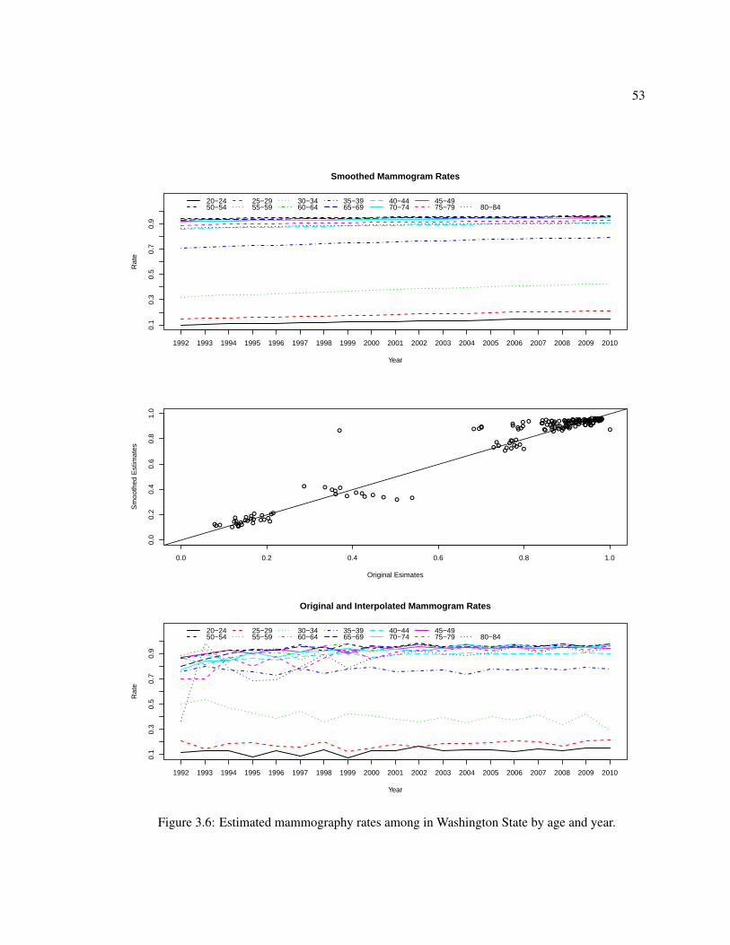
53
Smoothed Mammogram Rates
Year
Rat
e
1992 1993 1994 1995 1996 1997 1998 1999 2000 2001 2002 2003 2004 2005 2006 2007 2008 2009 2010
0.1
0.3
0.5
0.7
0.9
20−24 25−29 30−34 35−39 40−44 45−4950−54 55−59 60−64 65−69 70−74 75−79 80−84
●
●
●
●
●
●● ●●●●
●●
●
●
●
●
●
●● ●● ●●
●●
●
●
●
●
●
●●● ● ●●
●●
●
●
●
●
●
●●●● ●●
●●
●
●
●
●
●
●● ●● ●●
●●
●
●
●
●
●
●●● ● ●●
●●
●
●
●
●
●
●●● ●●●
●●
●
●
●
●
●
●●● ●● ●
●●
●
●
●
●
●
●●● ● ●●
●●
●
●
●
●
●
●●●●●●
●●
●
●
●
●
●
● ●●●● ●●
●
●
●
●
●
●
● ●●●● ●●
●
●
●
●
●
●
● ●●●●●●
●
●
●
●
●
●● ● ●●●●
●●
0.0 0.2 0.4 0.6 0.8 1.0
0.0
0.2
0.4
0.6
0.8
1.0
Original Esimates
Sm
ooth
ed E
stim
ates
Original and Interpolated Mammogram Rates
Year
Rat
e
1992 1993 1994 1995 1996 1997 1998 1999 2000 2001 2002 2003 2004 2005 2006 2007 2008 2009 2010
0.1
0.3
0.5
0.7
0.9
20−24 25−29 30−34 35−39 40−44 45−4950−54 55−59 60−64 65−69 70−74 75−79 80−84
Figure 3.6: Estimated mammography rates among in Washington State by age and year.

54
cancer example, the estimated ecological effects are smaller than the individual effects. For lung
cancer, the estimated ecological effect is smaller with the original and smoothed rates and larger
with the hybrid rates. In general we find some evidence that mammograms increase the risk of
being diagnosed with breast cancer, but we do not see the strong lung cancer-smoking relationship
that we might expect. Using hybrid rates, the posterior median for the relative risk associated with
getting a mammogram is exp(0.561) = 1.753, which means that the risk of being diagnosed with
breast cancer is 1.75 times larger if a woman has had a mammogram. If the age, period, and co-
hort terms are zero, then the probability of being diagnosed with breast cancer increases from about
0.001 to 0.002.
We may be able to detect a smoking-lung cancer relationship with a different summary of smok-
ing history. While it is well established that smoking increases the risk of lung cancer, this risk
decreases steadily after quitting smoking and increases in the number of cigarettes smoked [Freed-
man et al., 2008]. Thus, appropriately lagged measurements of the smoking rates may be more
predictive of lung cancer rates. For example, Henley et al. [2011] use 5-year lagged rates for current
smokers as well as “quit ratios” (the ratio of the number of people who have ever smoked to the
number of people who are former smokers).
Original Smoothed HybridAggregate Ecological Aggregate Ecological Aggregate Ecological
λ0 -6.256 -6.206 -6.350 -6.087 -6.548 - 6.379λ1 0.198 0.134 0.306 -0.025 0.565 0.364
(CI) (-0.071, 0.525) ( -0.118, 0.387) (-0.6133,1.086) (-0.999, 0.861) (0.096,1.029) (0.028, 0.702)
σα 0.127 0.184 0.176 0.197 0.173 0.182σβ 0.006 0.016 0.013 0.016 0.013 0.016σz 0.061 0.070 0.071 0.070 0.070 0.070
Table 3.9: Posterior estimates for the regression parameters and the variance terms for the aggregateand ecological models for breast cancer under different estimates for mammography rates. The λ0and λ1 rows are posterior means, and the credible intervals are 95% quantile-based intervals. Thepoint estimates for the standard deviations are posterior medians.
One striking feature of the results is that the credible intervals are much wider when using the
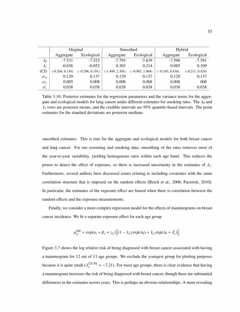
55
Original Smoothed HybridAggregate Ecological Aggregate Ecological Aggregate Ecological
λ0 -7.531 -7.523 -7.793 -7.639 -7.596 -7.591λ1 -0.036 -0.052 0.303 0.214 0.085 0.109
(CI) (-0.204, 0.130) ( -0.296, 0.191) (-1.499, 2.305) ( -0.983, 1.404) ( -0.245, 0.436) (-0.211, 0.429)
σα 0.129 0.137 0.129 0.137 0.128 0.137σγ 0.005 0.008 0.008 0.008 0.008 008σz 0.038 0.038 0.038 0.038 0.038 0.038
Table 3.10: Posterior estimates for the regression parameters and the variance terms for the aggre-gate and ecological models for lung cancer under different estimates for smoking rates. The λ0 andλ1 rows are posterior means, and the credible intervals are 95% quantile-based intervals. The pointestimates for the standard deviations are posterior medians.
smoothed estimates. This is true for the aggregate and ecological models for both breast cancer
and lung cancer. For our screening and smoking data, smoothing of the rates removes most of
the year-to-year variability, yielding homogenous rates within each age band. This reduces the
power to detect the effect of exposure, so there is increased uncertainty in the estimates of λ1.
Furthermore, several authors have discussed issues relating to including covariates with the same
correlation structure that is imposed on the random effects [Reich et al., 2006, Paciorek, 2010].
In particular, the estimates of the exposure effect are biased when there is correlation between the
random effects and the exposure measurements.
Finally, we consider a more complex regression model for the effects of mammograms on breast
cancer incidence. We fit a separate exposure effect for each age group
µaggi j = exp(αi + β j + zi j)
[(1 − xi j) exp(λ0) + xi j exp(λ0 + λi
1)].
Figure 3.7 shows the log relative risk of being diagnosed with breast cancer associated with having
a mammogram for 12 out of 13 age groups. We exclude the youngest group for plotting purposes
because it is quite small (λ(25,30]1 = −7.21). For most age groups, there is clear evidence that having
a mammogram increases the risk of being diagnosed with breast cancer, though there are substantial
differences in the estimates across years. This is perhaps an obvious relationships. A more revealing

56
analysis would examine whether mammograms increase the chances of early detection of breast
cancers or decrease breast cancer mortality.
3.7 Discussion and Conclusions
In this chapter we used the age-period-cohort model to fit and forecast rates for breast cancer and
lung cancer in Washington State. We also derived the appropriate mean model for including the pro-
portion exposed within each group in the APC model. We confirmed that age is the most prominent
time scale along which incidence rates change, but we also found that year of diagnosis (i.e., period)
is important for breast cancer and that year of birth (i.e., cohort) is important for lung cancer rates.
We found that more parsimonious models are superior in terms of mean squared error of forecasted
counts. We did not find strong evidence for the lung cancer–smoking relationship with these data,
but we did find that mammograms are associated with increase risk of a breast cancer diagnosis.
As mentioned in the introduction, the ultimate goal of this analysis is to extend the temporal
models discussed in this chapter to include the spatial origins of the cases, aggregated at the county
level. Riebler et al. [2012] have developed a correlated APC model for small numbers of areas,
and Lagazio et al. [2003] introduced a spatial APC model that includes space-time interaction terms
based on the framework of Knorr-Held [2000]. Extending to space presents several challenges but
may be beneficial for estimating the effects of certain exposures because there will be more hetero-
geneity in the exposure measurements. However, including mammography and smoking rates in
county-level models is challenging because the number of individuals sampled in each age × county
group can be very small or even zero, and so some form of modeling of the exposure rates will be
required. Furthermore, there will undoubtedly be a mismatch between the scale of the spatial het-
erogeneity in the exposure and units of aggregation. For example, cancer screening rates may differ
by hospital or regional health center, and the de facto catchment areas of these facilities do not, in
general, coincide with counties. Similarly, incorporating lagged measurements of tobacco use will
require strong assumptions about the stability of the population, and these assumptions are likely
violated. For example, there may be substantial inter county migration, especially among younger
age groups. Thus, smoking rates estimated from people living in a particular county at time t − 5

57
Posterior Means and 95% intervals for Log Relative Risk from Mammograms
Log Relative Risk (λ1)
Age
Ban
d
−2.0 −1.5 −1.0 −0.5 0.0 0.5 1.0 1.5 2.0
(30,
35]
(35,
40]
(40,
45]
(45,
50]
(50,
55]
(55,
60]
(60,
65]
(65,
70]
(70,
75]
(75,
80]
(80,
85]
85+
Figure 3.7: Log relative risks due to mammograms by age.

58
may not reflect the smoking histories of those living in the county at time t.
A second extension is to project full profiles with corresponding estimates of uncertainty in these
projections. In this chapter, we forecasted three years ahead as part of assessing model fit, but the
population values used to generate forecasts were fixed. For projections of future years, the popu-
lation sizes will also be estimates . Point estimates of population by age and sex in future years are
available from the Census Bureau and various state agencies at the state level but not at the county
level. Figures A.4-A.9 in appendix A show projected incidence for 2011-2015 using point estimates
of the population in from Washington State Office of Financial Management. Incorporating uncer-
tainty in both the population forecasts and disease rates is desirable for full probabilistic projection
of disease incidence or mortality.

59
Chapter 4
RESTRICTED COVARIANCE PRIORS FOR SPATIAL RANDOM EFFECTS
4.1 Introduction
The risk of disease inherently varies in space because risk factors are non uniformly distributed in
space. Such risk factors may include lifestyle variables such as alcohol and tobacco use or exposure
levels of environmental causes of disease such as air pollution or UV radiation. We expect that these
risk factors are positively correlated in space meaning that nearby areas will have similar exposure
levels or underlying characteristics.
In many studies, underlying disease risk factors are unknown or unmeasured. Bayesian mod-
els account for unknown or unmeasured risk factors using priors chosen to mimic their correlation
structure. The most common Bayesian framework for spatial count data uses Gaussian random ef-
fects with a covariance structure that imposes positive spatial dependence between random effects
of neighboring or near-by areas [Besag et al., 1991, Diggle et al., 1998, Banerjee et al., 2004]. The
non-Gaussian spatial clustering and Potts model based priors also impose positive dependence in the
relative risks of neighboring areas [Knorr-Held and Best, 2001, Green and Richardson, 2002]. More
recently, several authors have developed modifications to existing models specifically to preserve
positive dependence for spatial statistics applications [Wang and Pillai, 2013, Hughes and Haran,
2013].
We present a Bayesian model for area-level count data that uses Gaussian random effects with
a novel type of G-Wishart prior on the inverse variance-covariance matrix. The usual G-Wishart or
hyper inverse Wishart prior restricts off-diagonal elements of the precision matrix to 0 according to
the edges in an undirected graph [Dawid and Lauritzen, 1993, Roverato, 2002]. Dobra et al. [2011]
show that the flexibility of the G-Wishart prior has advantages over a more traditional conditional
autoregressive prior in a multivariate disease mapping setting. However, the G-Wishart prior allows

60
for both positive and negative conditional associations between neighboring areas.
The negative G-Wishart distribution that we introduce only has support over precision matrices
that lead to positive conditional associations. We describe Markov chain Monte Carlo (MCMC)
algorithms for this new prior and construct a Bayesian hierarchical model for areal count data that
uses the negative G-Wishart prior for the precision matrix of Gaussian random effects. We show
via simulation studies that risk estimates based on a model using the negative G-Wishart prior are
better than those based on conditional autoregression when the outcome is rare and the risk surface
is not smooth. Finally, we illustrate the improvement of our modification (measured via cross vali-
dation) in a multivariate application using cancer incidence data from the Washington State Cancer
Registry.
The structure of this chapter is as follows. In section 4.2 we present our modeling framework
and give a brief overview of conditional autoregressive models. In section 4.3 we define the negative
G-Wishart distribution and give the details of an MCMC sampler for estimating relative risks in a
spatial statistics context. In section 4.4 we present a simulation study based on univariate disease
mapping using the geography of the counties of Washington State. Finally in section 4.5 we ex-
tend the univariate negative G-Wishart model to multivariate disease mapping using the separable
Gaussian graphical model framework of Dobra et al. [2011].
4.2 Background
4.2.1 Notation
We use the same basic framework introduced in chapter 1. Let A = {A1, . . . An} be a set of non-
overlapping geographical areas and let y = {y1, . . . , yn} represent the set of counts of the observed
number of health events in these areas. Possible health events include deaths from a disease, incident
cases of a disease, or hospital admissions with specific symptoms of a disease. Next, let E =
{E1, . . . , En} be the set of expected counts and X = {x1 . . . xn} be a matrix where xi is a vector of
suspected risk factors measured in area i. Recall (section 1.2) that a generic Bayesian hierarchical

61
model for data of this type is
yi | y−i, Ei, θi ∼ Poi(Eiθi),
log(θi) = xTi β + ui,
π(u) = H,
where y−i is the vector of counts with area i excluded and H is a probability distribution with
spatial structure. Most choices of H encode the belief that the residual spatial random effects,
u, of near-by areas have similar values. The inclusion of H produces smoother (though biased)
estimates of the vector of relative risks, θ, with reduced variability (on average) compared to the
maximum likelihood estimates θ = y/E. These maximum likelihood estimates, called standardized
incidence ratios (SIRs) or standardized mortality ratios (SMRs), have large sampling variances when
the expected counts are small. A key task in modeling areal count data is to choose a prior H that is
flexible enough to adapt to the smoothness of the risk surface.
4.2.2 Existing Models for Areal Count Data
The most common choice for H is the Gaussian conditional autoregression or CAR prior introduced
in chapter 2. Recall that the CAR model is specified through a set of full conditional distributions.
The conditional distribution for the random variable, ui, given the other variables, u−i, is
ui | u−i ∼ N
∑j: j,i
bi ju j, τ2i
.The joint distribution of the vector u is a mean-zero multivariate normal distribution with precision
D−1(I − B), where Bi j = bi j, Bii = 0, and Dii = τ2i .
The intrinsic conditional autoregression or ICAR prior is the most commonly used prior for

62
spatial random effects within the class of CAR priors. The full conditionals of the ICAR prior are
ui | u−i ∼ N
1ωi+
∑j: j,i
ωi ju j,τ2
u
ωi+
. (4.1)
Here ωi j is nonzero if regions i and j are neighbors (i.e. share a border) and 0 otherwise; ωi+ is the
sum of all of the weights for a specific area. In the binary specification, ωi j = 1 for neighboring
regions and ωi+ = ni, the number of regions that border area i. Besag et al. [1991] use the ICAR
prior for spatial random effects in a disease mapping context in what has become known as the
convolution model:
log(θi) = xTi β + vi + ui.
Here vi is a non-spatial random effect and ui is a spatial random effect. The prior for v is N(0, σ2vI),
and the prior for u is the ICAR prior.
Though popular, the convolution model has several drawbacks. First, there are only two param-
eters (σ2v and τ2
u) to control the level of smoothing with only one of these (τ2u) contributing to the
spatial portion of the model. Second, the ICAR prior is improper. The joint distribution implied
by the conditional specification in (4.1) is a singular multivariate normal distribution with precision
matrix τ2u(Dω −W), where Dω is a diagonal matrix with elements Dii = ωi+. Since each row of
Dω −W sums to 0, this precision matrix does not have full rank, and the joint prior for u is im-
proper.
One way to alleviate both of these issues is through the addition of a spatial autocorrelation
parameter ρ:
ui | u−i ∼ N
ρ 1ωi+
∑j: j,i
ωi ju j,σ2
u
wi+
.This specification is called the proper CAR because it gives rise to a proper joint distribution as long
as ρ is between the reciprocals of the largest and smallest eigenvalues of D−1/2ω WD−1/2
ω [Banerjee

63
et al., 2004]. For the binary specification of W, this always includes ρ ∈ [0, 1). There are drawbacks
with the proper CAR when it comes to the relationship between ρ and the overall level of spatial
smoothing. The prior marginal correlations between the random effects of neighboring areas in-
crease very slowly as ρ increases, with substantial correlation obtained only when ρ is very close to
1 [Besag and Kooperberg, 1995]. Further, as ρ increases, the ordering of all pairwise marginal corre-
lations may change [Wall, 2004]. That is, for some value of ρ we may have cor(u1, u2) < cor(u3, u4)
and for a different ρ, cor(u3, u4) < cor(u1, u2).
4.3 Methodology
An alternative to specifying the prior for spatial random effects based on a set of conditional dis-
tributions is to work directly with the joint distribution. A Gaussian graphical model or covariance
selection model is a set of joint multivariate normal distributions that obey the pairwise condi-
tional independence properties encoded by an undirected graph, G [Dempster, 1972, Lauritzen,
1996]. This graph has two elements: the vertex set V and the edge list E (see section 2.1) .
The absence of an edge between two vertices corresponds to conditional independence and im-
plies a specific structure for the precision matrix of the joint distribution. If u follows a multi-
variate normal distribution with precision matrix K, then u follows a Gaussian graphical model if
ui ⊥⊥ u j | uV\(i, j) ⇐⇒ (i, j) < E =⇒ Ki j = 0 for any pairs i and j. Here uV\(i, j) is the vector u
excluding the ith and jth elements.
The conjugate prior for the precision matrix in the Gaussian setting is the Wishart distribution,
which is a distribution over all symmetric, positive definite matrices of a fixed dimension. The
Wishart distribution has two parameters. The first is a scaler δ > 2, which controls the spread of the
distribution. The second is an n×n matrix D, which is related to the location of the distribution. For
K ∼ Wis(δ,D), E(K) = (δ+ n−1)D−1 and mode(K) = (δ−2)D−1. The G-Wishart distribution is the
hyper Markov, conjugate prior for the precision matrix in a Gaussian graphical model [Dawid and
Lauritzen, 1993, Roverato, 2002]. The G-Wishart distribution is a distribution over P+(G), the set
of all symmetric, positive definite matrices with zeros in the off-diagonal elements that correspond

64
to missing edges in G. The density of the G-Wishart distribution for a matrix K is
Pr(K | δ,D,G) =1
IG(δ,D)|K|(δ−2)/2 exp
(−
12〈K,D〉
)1K∈P+(G), (4.2)
where 〈A, B〉 is the trace of AT B. The normalizing constant IG(δ,D) has a closed form when G
is a decomposable graph and can be estimated for general graphs using the Monte Carlo method
proposed by Atay-Kayis and Massam [2005].
4.3.1 Negative G-Wishart Distribution
We propose a new G-Wishart distribution called the negative G-Wishart distribution that imposes
additional constraints on K. This is a distribution over positive definite matrices where the off-
diagonal elements that correspond to (non-missing) edges in E are less than 0. This restriction
means that all pairwise conditional (or partial) correlations are positive because
cor(ui, u j | uV\{i, j}
)=−Ki j√KiiK j j
.
This restriction is attractive in a spatial statistics context where we believe neighboring areal units
are likely to be similar to each other, given the other areas.
If K is a negative G-Wishart variate, then
Pr(K | G, δ,D, 0) =1
IG(δ,D, 0)|K|(δ−2)/2 exp
(−
12〈K,D〉
)1K∈P+(G)∩S0 . (4.3)
Here IG(δ,D, 0) is the unknown normalizing constant, and S0 is the orthant of R12 (n2+n) where n
elements are strictly positive and 12 n(n − 1) elements are less than 0. The normalizing constant in
(4.2) is finite as long as δ > 2 and D−1 ∈ P+(G) [Atay-Kayis and Massam, 2005]. The normalizing
constant in (4.3) will be finite under the same conditions because the support of the negative G-
Wishart is a subset of the support of the G-Wishart distribution. The mode of the negative G-Wishart
is again (δ − 2)D−1, and for this reason we only consider D−1 ∈ P+(G) ∩ S0. We write NWisG for
the negative G-Wishart distribution and WisG for the G-Wishart distribution.

65
Atay-Kayis and Massam [2005] and Dobra et al. [2011] transform K to the Cholesky square
root, which we callΦ, because it is easier to handle the positive definite constraint in the transformed
space. In the G-Wishart case, the elements ofΦ are either variation independent or are deterministic
functions of other elements. We call the off-diagonal elements ofΦ that correspond to missing edges
in the graph G “non-free.” These are deterministic functions of the “free” elements: the diagonal
elements and the off-diagonal elements corresponding to edges in G. If we restrict K to the space
P+(G) ∩ S0, we have the following constraints on the off-diagonal elements of the Cholesky square
root Φ:
Φii > 0 for i = 1, . . . , n (4.4)
Φi j = −1
Φii
i−1∑d=1
ΦdiΦd j for (i, j) < E (4.5)
Φi j < −1
Φii
i−1∑d=1
ΦdiΦd j for (i, j) ∈ E (4.6)
The first two conditions guarantee that ΦTΦ ∈ P+(G). The addition of the third inequality guaran-
tees that ΦTΦ ∈ S0; however, this restriction comes at the cost of losing variation independence.
4.3.2 Sampling from the Negative G-Wishart Distribution
We sample from the negative G-Wishart distribution using a random walk Metropolis-Hastings al-
gorithm similar to the sampler proposed by Dobra et al. [2011]. We sequentially perturb one free
elements Φi0 j0 at a time, holding the other free elements constant. In doing so, we must find the
support of the conditional distribution of Φi0 j0 given the other elements. The support of this condi-
tional distribution is the set of Φi0 j0 that satisfy inequalities (4.4)-(4.6) when the free elements, the
left hand sides of (4.4) and (4.6), are fixed.
For each specific graph and fixed pair (i0, j0), we can write the inequalities in (4.6) as
Φi j < gi j(Φi0 j0 ,F−(i, j)) for (i, j) ∈ E,

66
where F−(i, j) is the set of fixed, free elements of Φ excluding Φi j and Φi0 j0 . We construct gi j by
substituting the equalities from (4.5) for all of the non-free elements that depend on Φi0 j0 . Each g
is (at worst) a quadratic function of Φi0 j0 . When g is a linear function, solving g for Φi0 j0 gives a
solution set of the form g−1i j (Φi j,F−(i, j)) = {Φi0, j0 ∈ (Li j,∞)} where Li j < 0. When g is quadratic,
the solution set is g−1i j (Φi j,F−(i, j)) = {Φi0 j0 ∈ (Li j,Ui j)} where Li j is again negative.
If (i, j) ≺ (i0, j0) in lexicographical order, then the upper bound for Φi j cannot depend on Φi0 j0 .
Depending on the graphical structure, there are pairs (i, j) � (i0, j0) such that the bound for Φi j does
not depend on Φi0 j0 . In these cases g−1i j (Φi j,F−(i, j)) = (−∞,∞).
Theorem 1 The conditional distribution of a free element Φi0 j0 , i0 , j0 given all other free elements
is a continuous distribution over an open subinterval of R− given by
⋂(i, j)∈E
g−1i j (Φi j,F−(i, j)) ∩ (−∞,
−1Φi0i0
i0−1∑d=1
Φdi0Φd j0)
The analogous theorem for free, diagonal elements is
Theorem 2 The conditional distribution of a free element Φi0i0 given other free elements is a con-
tinuous distribution over a subinterval of R+ given by
Φi0i0 ∈
maxi0<k≤p,(i0,k)∈E
−∑i0−1
d=1 Φdi0Φdk
Φi0k
,∞ for 1 < i0 < n,
Φi0i0 ∈ (0,∞) for i0 = 1, n.
For proofs, see appendix B.
We use these bounds to construct a Markov Chain with stationary distribution equal to the
negative G-Wishart distribution. Suppose Φt is an upper-triangular matrix at iteration t such that
(Φt)TΦt ∈ P+(G) ∩ S0. For each free element in Φti0 j0
do the following:
1. Calculate the upper and lower limits for Φti0 j0
as described above.
2. Sample from a truncated normal with these limits, mean Φti0 j0
, and standard deviation σm.

67
3. Update the non-free elements in lexicographical order. These steps give a proposal K′ =
(Φ′)TΦ′ where the free elements in Φ′ are equal to the free elements of Φt except in the
(i0, j0) entry.
4. Accept according to the acceptance probability min(1,RΦ), where
RΦ =π(K′ | D, δ,G)q(Kt | K′)π(Kt | D, δ,G)q(K′ | Kt)
=
Φ′i0i0
Φti0i0
δ+νi(G)−1
exp(−
12
⟨K′ −Kt,D
⟩) TNorm(Φti0 j0
; Φ′i0 j0, σm, li0 j0 , ui0 j0)
TNorm(Φ′i0 j0; Φt
i0 j0, σm, li0 j0 , ui0 j0)
.
TNorm(·; µ, σ, l, u) is the density of a normal distribution with mean µ and standard deviation σ
truncated to the interval (l, u), and νi(G) is the number of areas that are neighbors of area i but have
larger index numbers. That is νi(G) = #{ j : ωi j = 1 and i < j}.
4.3.3 Using the Negative G-Wishart in a Hierarchical Model
We the use negative G-Wishart prior within the generic Bayesian hierarchical model for areal counts
given in section 4.2:
log(θi) = xTi β + ui,
π(u | α, τu,K) = N(α1, (τ2
uK)−1),
π(α) = N(0, σ2α),
π(β) = N(0, σ2βI),
π(τ2u | a, b) = Gam(a, b),
π (K | G, δ,D) = NWisG (δ, (δ − 2)D(ρ)) with K11 = W1+,
D−1(ρ) = DW − ρW,
π(ρ) = Unif(0, 0.05, 0.1, . . . ,
0.8, 0.82, . . . , 0.90, 0.91, . . . , 0.99).

68
We suggest choosing the hyper parameters for the priors on α and τ2 by first specifying a rea-
sonable range for the average relative risk and then finding values of σ2α and (a, b) that match this
range for a fixed value of K. For fixed K, the distribution of u = 1/n∑n
i=1 ui is a univariate normal
distribution depending on α and τ2. Using the adjacency matrix of Washington State as an exam-
ple and letting K = D−1(0.99), 95% of the prior on exp(u) is between (1/8, 8) when σ2α = 1 and
(a, b) = (0.5, 0.0015). For a more informative prior, setting σ2α = 1/4 gives a range of (1/2, 2). More
details of this prior specification framework are in appendix B.
The discrete prior on the spatial autocorrelation parameter ρ was introduced by Gelfand and
Vounatsou [2003] for computational convenience and to reflect the fact that large values of ρ are
needed to achieve non-negligible spatial dependence in the proper CAR prior. Jin et al. [2007] use
a continuous uniform prior on (0, 1) and a Beta(18, 2) prior in a similar multivariate context. For
our purposes, using a discrete prior for ρ is essential for carrying out MCMC because ρ appears
in the normalizing constant of the prior on K. That is, the normalizing constant in (4.3) becomes
IG(δ,D(ρ), 0). As will be shown below, we pre-calculate ratios of these normalizing constants in
advance. It is not practical to repeat this process at each step of the MCMC.
We estimate the posterior distribution of the relative risks, θ, using MCMC. Most of the tran-
sitions are standard Metropolis or Gibbs updates (see appendix B) except for the updates on the
precision matrix K and the autocorrelation parameter ρ. We update K as described in section 4.3.2,
skipping over Φ11 to preserve the restriction on K11. We update ρ by choosing the next smallest or
largest value in {0, 0.05, 0.1, . . . , 0.8, 0.82, . . . , 0.90, 0.91, . . . , 0.99}, each with probability 1/2. If ρt
and ρ′ are not on the boundary of this list, then the acceptance probability is min(1,Rρ) where
log(Rρ) = −1/2tr[(δ − 2)K
{(Dw − ρ
′W)−1 − (Dw − ρtW)−1}]
(4.7)
+ log (IG(δ, (δ − 2)D(ρt), 0)) − log(IG(δ, (δ − 2)D(ρ′), 0)
).
If either ρt or ρ′ is on the boundary, there is an extra factor of 2 because the proposal is not sym-
metric: if ρt = 0, we propose ρ′ = 0.05 with probability 1. Because the graph G is constant, the
normalizing constants in (4.7) only depend on ρ. We estimate the necessary ratios of normalizing

69
constants and store them in a table prior to running the full MCMC.
For two densities of the form π1(η) = c1q1(η) and π2(η) = c2q2(η) with normalizing constants
c1 and c2, the ratio of normalizing constants is given by r = c1/c2 = E2[q1(η)/q2(η)
]when the
support of the two distributions are the same [Chen et al., 2000]. Here E2 is the expectation under
the second density. We estimate this expectation for each consecutive pair ρ1 > ρ2 using MCMC.
Here we give the details for estimating the normalizing constants of a set of G-Wishart distributions
without restrictions on the K11 element and with δ = 3. However, the same process will work for
the negative G-Wishart and with the restriction that K11 = W1+.
• Generate a Markov Chain K1, K2, . . .KS with stationary distribution WisG(3, (Dw−ρ2W)−1).
• For each state, let Zi = −1/2tr[Ki
((Dw − ρ1W)−1 − (Dw − ρ2W)−1
)].
• Estimate log[IG(3,D(ρ1))
]− log
[IG(3,D(ρ2))
]by log
[1S∑S
i=1 exp(Zi)].
For each pair (ρ1, ρ2), we average over the estimates from 10 parallel chains of 100, 000 iterations.
Figure B.1 in appendix B shows the evolution of the estimates of
log[IG(3, (Dw − 0.99W)−1)
]− log
[IG(3, (Dw − 0.98W)−1)
]using the adjacency graph of the counties in Washington State.
4.3.4 Multivariate Disease Mapping
In section 4.5, we use the negative G-Wishart prior to analyze incidence data from the Washington
State Cancer Registry. In doing so, we adopt the same framework as Dobra et al. [2011] and assign
a matrix normal prior to the log relative risks. We again assume there are n areas with counts for C
cancer sites observed in each area. If Y = {yic : i = 1, . . . , n, c = 1, . . . ,C} is a matrix of observed

70
counts and E = {Eic : i = 1, . . . , n, c = 1, . . . ,C} is a matrix of expected counts, then we have
yic|Eic, θic ∼ Poi (Eicθic) ,
log(Θ) = U,
U ∼ MN(M,K−1
C ,K−1R
),
Mc ∼ N(0, σ2
M
)for c = 1, . . .C,
KC ∼ Wis (δC , (δC − 2)DC) or WisGC (δC , (δC − 2)DC) ,
KR ∼ NWisGR
(δR, (δR − 2)D−1
R
).
We use MN(M,ΣC ,ΣR) to denote the matrix normal distribution with separable covariance structure
[Dawid, 1981]. That is vec (U) | M,ΣR,ΣC ∼ N (vec {M} ,ΣC ⊗ ΣR), where “⊗” is the Kronecker
product.
In the absence of any information on cancer risk factors such as smoking rate or a socioeconomic
summary measure, we only include an overall rate for each cancer in the mean model. That is,
Mic = Mc. The row covariance ΣR describes the spatial covariance structure of the log relative risks.
The column covariance matrix ΣC describes the covariance between the cancers.
We incorporate the negative G-Wishart distribution as the prior for the spatial precision matrix
Σ−1R = KR and we use a G-Wishart or Wishart prior with mode equal to the identity matrix for
Σ−1C = KC . When the prior on KC is a G-Wishart prior, we incorporate uncertainty in the between-
cancer conditional independence graph GC using a uniform prior over all graphs. For both priors,
we restrict (KC)11 = 1 for identifiability. Finally, we use an independent normal prior on each Mc.
We estimate the relative risks under this model using an MCMC sampler identical to that in Dobra
et al. [2011], substituting in the sampler from section 4.3.2 for the update on KR.
4.4 Simulation Study
We compare the univariate disease mapping model using the negative G-Wishart prior to three other
models in a simulation study based on a study in Lee et al. [2014].
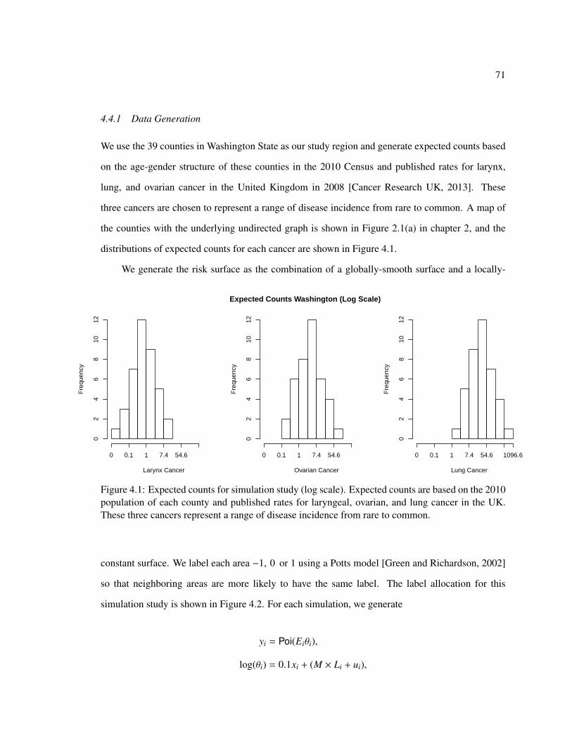
71
4.4.1 Data Generation
We use the 39 counties in Washington State as our study region and generate expected counts based
on the age-gender structure of these counties in the 2010 Census and published rates for larynx,
lung, and ovarian cancer in the United Kingdom in 2008 [Cancer Research UK, 2013]. These
three cancers are chosen to represent a range of disease incidence from rare to common. A map of
the counties with the underlying undirected graph is shown in Figure 2.1(a) in chapter 2, and the
distributions of expected counts for each cancer are shown in Figure 4.1.
We generate the risk surface as the combination of a globally-smooth surface and a locally-
Larynx Cancer
Fre
quen
cy
0 0.1 1 7.4 54.6
02
46
810
12
Ovarian Cancer
Fre
quen
cy
0 0.1 1 7.4 54.6
02
46
810
12
Lung Cancer
Fre
quen
cy
0 0.1 1 7.4 54.6 1096.6
02
46
810
12
Expected Counts Washington (Log Scale)
Figure 4.1: Expected counts for simulation study (log scale). Expected counts are based on the 2010population of each county and published rates for laryngeal, ovarian, and lung cancer in the UK.These three cancers represent a range of disease incidence from rare to common.
constant surface. We label each area −1, 0 or 1 using a Potts model [Green and Richardson, 2002]
so that neighboring areas are more likely to have the same label. The label allocation for this
simulation study is shown in Figure 4.2. For each simulation, we generate
yi = Poi(Eiθi),
log(θi) = 0.1xi + (M × Li + ui),

72
where Li is the label assigned to county i. We simulate xi and ui independently from multivariate
normal distributions with Matern covariance function, smoothness parameter 2.5 and range chosen
so that the median marginal correlation is 0.5. Thus, each of the vectors x and u are realizations
of a smooth spatial process observed at a finite set of points. In different simulations, we set M to
0.5, 1, or 1.5. Larger values of M lead to a risk surface with more discontinuities. We generate 50
realizations from each combination of M and the three sets of expected counts.
In the simulation study described below, we run each chain for 100, 000 iterations, discarding
−1 0 1
Figure 4.2: Labels (Li) for simulation study
the first half as burn in. We set the prior parameters for the model in section 4.3.3 to σα = 1,
σβ = 10, (a, b) = (0.5, 0.0015), and δ = 3. Figures B.2 and B.3 in appendix B shows the evolution
of the posterior mean for 10 different chains for two elements of the Cholesky square root and two
random effects. In all cases, we reach convergence in about 10, 000 iterations.
4.4.2 Results
We compare the model using the negative G-Wishart prior to three other models. The model using
the G-Wishart prior is identical to the model from section 4.3.3 except that the prior on the precision

73
matrix K is the G-Wishart prior instead of the negative G-Wishart prior. We also compare against
the convolution model from section 4.2 and a similar model that includes only spatial random effects
with an ICAR prior. The ICAR only model is not generally used in practice because there is no way
to account for non spatial heterogeneity. For the convolution and ICAR models, we estimate the
posterior mean and variance of the relative risks using INLA [Rue et al., 2009]. For the models using
negative G-Wishart and G-Wishart priors, we explore the posterior distributions using MCMC.
We compare the four methods using the root-averaged mean squared error (RAMSE) of the
posterior mean of each relative risk θi. This is the square root of the mean squared error averaged
over all simulations and all areas. For S simulations and B iterations of the MCMC, the RAMSE is
RAMSE =
√√√1
39 × S × B
39∑i=1
S∑s=1
B∑b=1
(θ(b)is − θis)2,
where θis it the true relative risk for area i in simulation s and θ(b)is is the corresponding value at
iteration (b) of the MCMC. The results of this simulation are shown in Figure 4.3, and the triangle
indicates the lowest RAMSE within each scenario.
In general, the RAMSE decreases for all four models when the expected counts increase, and the
RAMSE increases when the level of smoothing decreases (i.e. M increases). The model using the
negative G-Wishart prior performs the best in six out of nine scenarios, and we see the greatest ben-
efit in the larynx, M = 1.5 simulation when the expected counts are low and the local discontinuities
in the risk surface are most prominent.

74
Larynx
RA
MS
E
NG
W
GW
BY
M
ICA
R
NG
W
GW
BY
M
ICA
R
NG
W
GW
BY
M
ICA
R
2.0
2.5
3.0
3.5
M = 0.5 M = 1 M = 1.5M = 0.5 M = 1 M = 1.5
Ovarian
RA
MS
E
NG
W
GW
BY
M
ICA
R
NG
W
GW
BY
M
ICA
R
NG
W
GW
BY
M
ICA
R
0.75
1.25
1.75
2.25 M = 0.5 M = 1 M = 1.5M = 0.5 M = 1 M = 1.5
Lung
RA
MS
E
NG
W
GW
BY
M
ICA
R
NG
W
GW
BY
M
ICA
R
NG
W
GW
BY
M
ICA
R
0.50
0.55
0.60
0.65 M = 0.5 M = 1 M = 1.5M = 0.5 M = 1 M = 1.5
Figure 4.3: Root average mean squared error (RAMSE) for relative risks θ. The triangle signifiesthe smallest value for each experiment. The four models are NGW (negative G-wishart prior onprecision matrix for spatial random effects), GW (G-wishart prior on precision matrix for spatialrandom effects), BYM (convolution model with independent and ICAR random effects), ICAR (onlyICAR random effects). All models show increased RAMSE with increased spatial discontinuities(large M) and increased RAMSE with smaller expected counts. The NGW prior performs the bestin six out of nine scenarios with the greatest benefit in the larynx, M = 1.5 experiment.

75
4.5 Multiway Disease Mapping
In this section we use the negative G-Wishart prior in a multivariate disease mapping context using
cancer incidence data from the Washington State Cancer Registry. Let Y = {yic : i = 1, . . . , 39, c =
1, . . . , 10} be an 39 × 10 matrix of incidence for 10 cancers in each county in Washington State in
2010. These 10 cancers have the largest incidence across the state in 2010. The expected counts Eic
are calculated separately for each cancer using internal standardization based on sex and quintenial
age bands. The standardized incidence ratios (SIRs = Y/E) for these data are between 0 and 3.91,
and the range of the empirical correlations between the SIRs of the different cancers (not taking into
account spatial dependence) is (−0.203, 0.477). Just over 20% of the counts are under 5, but we do
not treat small counts as missing in this analysis.
We use cross validation to compare the model in section 4.3.4 to models using the G-Wishart
prior [Dobra et al., 2011] and using the proper CAR form for KR [Gelfand and Vounatsou, 2003].
We compare 3 different choices for the prior on KR and two choices for the prior on KC . For the
negative G-Wishart and G-Wishart priors on KR, we set δR = 3 and DR = D(ρ) = (Dω − ρW)−1,
where the prior on ρ is the same as in section 4.3.3. The MCAR prior on KR is simply KR = D(ρ)−1.
In the absence of nay information on the correlation between cancers, we choose a diagonal matrix
for DC for both the Wishart and the G-Wishart priors on KC . Jin et al. [2007] suggest using a data
driven prior where the diagonal elements of DC are set based on univariate analyses for each cancer.
Here we follow Dobra et al. [2011] and set δC = 3 and DC = I. We set the prior variance of the
mean rates {M1,M2 . . . MC}T to σ2
M = 1/4. Alternatively, we could use data driven priors based on
the range of the SIRs to set σ2M.
We randomly split all observations into 10 bins and create 10 data sets, each with one bin of
counts held out. We impute the missing counts as part of the MCMC and compare the models based
on average predictive squared bias (BIAS2) and average predictive variance (VAR). Let EM(Yic) be
the predicted value under modelM, varM(Yic) be the variance of the posterior predictive distribu-
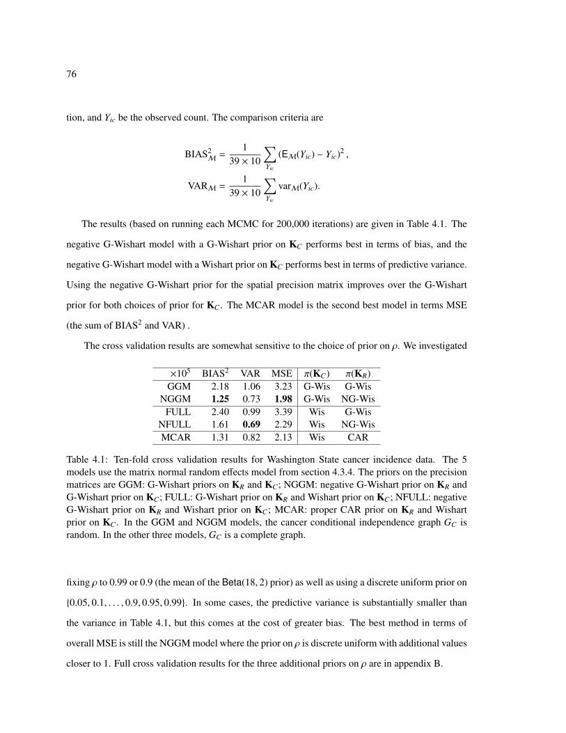
76
tion, and Yic be the observed count. The comparison criteria are
BIAS2M
=1
39 × 10
∑Yic
(EM(Yic) − Yic)2 ,
VARM =1
39 × 10
∑Yic
varM(Yic).
The results (based on running each MCMC for 200,000 iterations) are given in Table 4.1. The
negative G-Wishart model with a G-Wishart prior on KC performs best in terms of bias, and the
negative G-Wishart model with a Wishart prior on KC performs best in terms of predictive variance.
Using the negative G-Wishart prior for the spatial precision matrix improves over the G-Wishart
prior for both choices of prior for KC . The MCAR model is the second best model in terms MSE
(the sum of BIAS2 and VAR) .
The cross validation results are somewhat sensitive to the choice of prior on ρ. We investigated
×105 BIAS2 VAR MSE π(KC) π(KR)GGM 2.18 1.06 3.23 G-Wis G-Wis
NGGM 1.25 0.73 1.98 G-Wis NG-WisFULL 2.40 0.99 3.39 Wis G-Wis
NFULL 1.61 0.69 2.29 Wis NG-WisMCAR 1.31 0.82 2.13 Wis CAR
Table 4.1: Ten-fold cross validation results for Washington State cancer incidence data. The 5models use the matrix normal random effects model from section 4.3.4. The priors on the precisionmatrices are GGM: G-Wishart priors on KR and KC; NGGM: negative G-Wishart prior on KR andG-Wishart prior on KC; FULL: G-Wishart prior on KR and Wishart prior on KC; NFULL: negativeG-Wishart prior on KR and Wishart prior on KC; MCAR: proper CAR prior on KR and Wishartprior on KC . In the GGM and NGGM models, the cancer conditional independence graph GC israndom. In the other three models, GC is a complete graph.
fixing ρ to 0.99 or 0.9 (the mean of the Beta(18, 2) prior) as well as using a discrete uniform prior on
{0.05, 0.1, . . . , 0.9, 0.95, 0.99}. In some cases, the predictive variance is substantially smaller than
the variance in Table 4.1, but this comes at the cost of greater bias. The best method in terms of
overall MSE is still the NGGM model where the prior on ρ is discrete uniform with additional values
closer to 1. Full cross validation results for the three additional priors on ρ are in appendix B.

77
Now we turn to results from fitting the complete data. Figure 4.4 shows the estimated posterior
distribution of the spatial autocorrelation parameter ρ for the five models. The posterior for ρ is
much more concentrated around small values when the prior on KR is a G-Wishart prior than with
a negative G-Wishart prior KR for both priors on KC . The posterior median for ρ when using CAR
prior on KR is between the estimates from the G-Wishart and negative G-Wishart priors. Figure
4.5 shows the estimated posterior probabilities of including edges in GC for two different priors on
KR. The upper and lower triangles are quite similar, indicating that inference on the between-cancer
conditional independence graph is not sensitive to the choice of prior on KR. The Lung-Leukemia,
Bladder-Non-Hodgkin lymphoma, and Colon-Breast cancer edges have the biggest posterior edge
inclusion probabilities.
Finally, Table 4.2 shows the average coverage and length of 95% posterior (in sample) predic-
tive intervals from fitting the GGM, NGGM and MCAR models once to the complete data. While
all models have the correct coverage, the posterior predictive intervals from the negative G-Wishart
model are slightly smaller. This remains true when averaging over the length of the predictive inter-
vals for small counts (≤ 5) or larger counts (≥ 20).
COV LEN LEN≤5 LEN≥20
GGM 0.959 31.33 7.47 51.82NGGM 0.954 31.27 7.36 51.79MCAR 0.956 31.31 7.41 51.85
Table 4.2: Nominal coverage rates (COV) and mean length (LEN) of the in-sample 95% credibleintervals. Mean lengths are also give by ranges of observed counts.
4.6 Discussion
This chapter presents a novel extension of the G-Wishart prior for the precision matrix of spatial
random effects. In a simulation study, the negative G-Wishart prior is able to better estimate the
relative risks when the outcomes are rare (i.e. the expected counts are small) and when the risk sur-
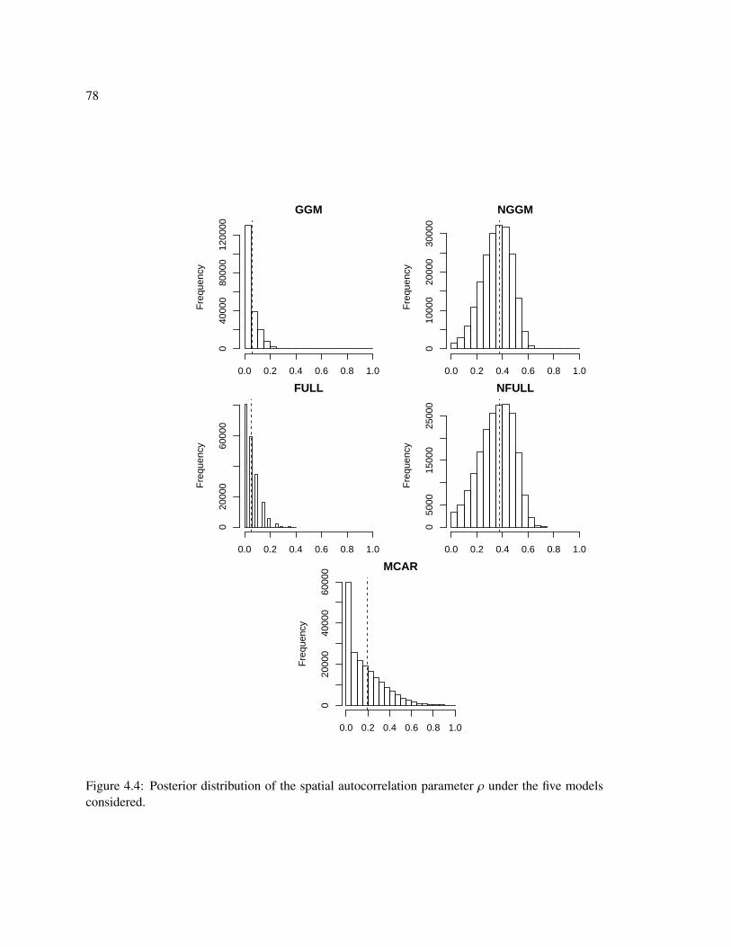
78
GGMF
requ
ency
0.0 0.2 0.4 0.6 0.8 1.0
040
000
8000
012
0000
NGGM
Fre
quen
cy
0.0 0.2 0.4 0.6 0.8 1.0
010
000
2000
030
000
FULL
Fre
quen
cy
0.0 0.2 0.4 0.6 0.8 1.0
020
000
6000
0
NFULL
Fre
quen
cy
0.0 0.2 0.4 0.6 0.8 1.0
050
0015
000
2500
0
MCAR
Fre
quen
cy
0.0 0.2 0.4 0.6 0.8 1.0
020
000
4000
060
000
Figure 4.4: Posterior distribution of the spatial autocorrelation parameter ρ under the five modelsconsidered.
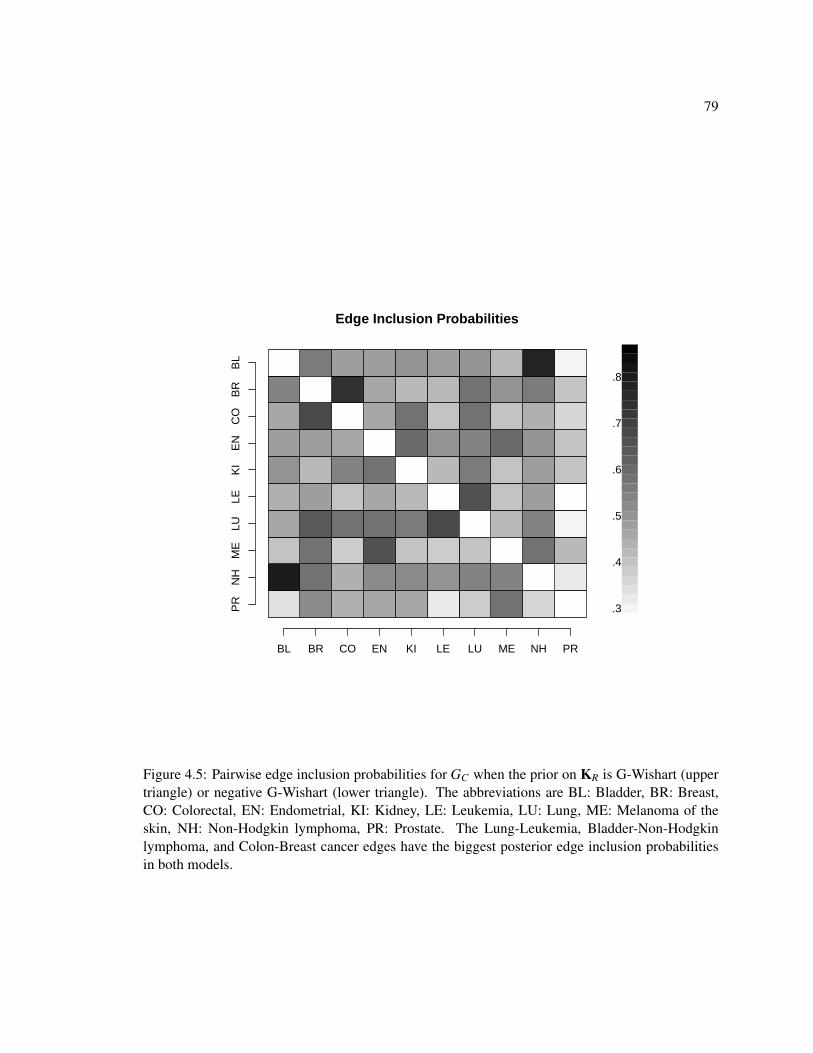
79
Edge Inclusion Probabilities
PR
NH
ME
LULE
KI
EN
CO
BR
BL
BL BR CO EN KI LE LU ME NH PR
0.3
0.4
0.5
0.6
0.7
0.8
Figure 4.5: Pairwise edge inclusion probabilities for GC when the prior on KR is G-Wishart (uppertriangle) or negative G-Wishart (lower triangle). The abbreviations are BL: Bladder, BR: Breast,CO: Colorectal, EN: Endometrial, KI: Kidney, LE: Leukemia, LU: Lung, ME: Melanoma of theskin, NH: Non-Hodgkin lymphoma, PR: Prostate. The Lung-Leukemia, Bladder-Non-Hodgkinlymphoma, and Colon-Breast cancer edges have the biggest posterior edge inclusion probabilitiesin both models.
80
face is not smooth. The restriction of the G-Wishart prior was shown to be advantageous when used
in a multivariate disease mapping context with incidence data from the Washington State Cancer
Registry.
There are a number of computation issues when using the negative G-Wishart and G-Wishart
priors. Each MCMC run for the univariate negative G-Wishart model in section 4.4 takes approxi-
mately 1.5 hours to complete on a 2.5GHz Intel Xeon E5-2640 processor, and, with the exception
of the MCAR model, the MCMC for each model in section 4.5 takes about 6.5 hours to complete.
In contrast, estimating the convolution and ICAR models from section 4.4 takes a matter of seconds
using INLA. We have found that the proposal variance for updates of the Cholesky square (section
4.3.3) and the random effects (see appendix B) must be chosen carefully to avoid poor convergence.
In both sections 4.4 and 4.5, we used s = 2 for updating Φ and s = 0.1 for updating u. While the
computation time for the models detailed here are not prohibitive, they may pose a challenge as we
extend to more complicated datasets, such as those including multiple diseases in time and space.

81
Chapter 5
BAYESIAN METHODS FOR SETS OF BINARY CONTINGENCY TABLES
5.1 Introduction
Data on individual health outcomes often include demographic or exposure information as well as
spatial or temporal information about the origin of each case. In many situations, the demographic
or exposure features can be represented as binary or categorical variables. If these data come from
distinct geographic locations (school districts, cities, counties), then the data form a set of multi-way
contingency tables, each associated with a spatial location. Further, the relationships between the
outcome and risk factors or the relationships between risk factors may differ by location if there
are unobserved confounding factors that vary in space. This heterogeneity may be in the form of
spatially-varying strengths of association (i.e., different parameter values for the same set of in-
teractions), or it may be in terms of different interaction models by location. To the best of our
knowledge, the current literature does not contain any statistical approach to account for both kinds
of heterogeneity for multiple contingency table data.
5.1.1 Background
Some of the earliest methods for the analysis of grouped categorical data date back to Goodman
[1973] and Clogg and Goodman [1984]. The former paper proposes a log-linear parameterization
for sets of multi-way contingency tables that allows for complete homogeneity, complete hetero-
geneity or partial heterogeneity among tables. However, the log-linear interaction terms being fitted
to each table are the same across tables–only their values are allowed to vary. The latter paper
extends the latent structure model of Goodman [1974] to multiple contingency tables. In a latent
structure model, the dependence between the observed variables is explained by membership in

82
latent classes. Conditional on the latent class, observed variables are independent. In Clogg and
Goodman [1984], heterogeneity across tables is captured by different class membership probabil-
ities for each table. This approach is also limited in the sense that the interaction structure is the
same across tables. Therefore the latent class approach has the same pitfall as Goodman [1973] with
the added complication of having to decide on the number of latent classes. Recently, Wall and Liu
[2009] introduced a spatial latent class model in which class membership probabilities for nearby
locations are more similar than class membership probabilities for distant locations. This approach
still assumes the same interaction structure within all latent classes, and the number of classes must
be pre-specified.
More recent papers that approach the analysis of sets of contingency tables can be found in the
ecological inference literature. Most of these efforts are limited to 2 × 2 tables and do not address
the crucial question of how to perform model selection. Many relevant papers in the ecological
inference literature [Haneuse and Wakefield, 2004, Wakefield, 2004, Jackson et al., 2008, Wakefield
et al., 2011] suggest a hierarchical model in which the individual-level data is modeled as a con-
volution of binomial distributions (or normal approximations to the binomial likelihood) with the
dependence among the binomial parameters captured in a second stage by some hyperparameters.
The choice of hyperparameters as well as the choice of corresponding priors for them differ from
author to author. However, none of these methods can identify areas for which should independence
be favored over dependence because the parameterization of the resulting hierarchical models does
not vary from area to area. This problem becomes even more serious when three or more categorical
variables are observed in each area. For example, Tassone et al. [2010] present a Bayesian hierarchi-
cal model for 25 tables in which first and second-order interaction terms are spatially varying while
higher order terms are fixed. Their approach is computationally slow (taking 7 days for the largest
model) and does not provide a framework for model selection.
In this chapter, we present a framework for a joint analysis of multiple contingency tables in the
presence of spatial association. Our methodology uses treed models to identify clusters of locations
that share the same dependenc patterns across multiple categorical variables. The clusters are gener-

83
ated in such a way that tables from neighboring locations have a higher probability of being assigned
to the same cluster. Thus, we can capture the spatial variation in risk factors while accounting for
the interactions among these factors.
5.1.2 Data
We demonstrate our method using North Carolina birth outcome data introduced in chapter 1. Each
birth record consists of five binary variables: low birthweight (1–less than 2500 grams, 2–at least
2500 grams), full term birth (1–less than 37 weeks gestational age, 2–at least 37 weeks), maternal
race (1–white/non Hispanic, 2–black/non Hispanic), infant sex (1–male, 2–female), and maternal
smoking (1–non smoker, 2–smoker). We can organize the data into separate 25 contingency tables
for each of the 100 counties based on the mother’s residence. The table totals ranging from 39 to
9850. There are a substantial number of sampling zeros (713) and counts less than 3 (1390) in these
tables. Thus, a Bayesian approach that allows for sharing of information between those counties
with small table totals is essential for estimating higher order interaction terms.
In this chapter, we do not make a distinction between outcomes and predictors. Instead, we
jointly model these five variables, and we can recover more familiar conditional probabilities and
odds ratios from our estimates of the joint distribution. This joint approach is well suited to these
data because two variables (low birthweight and full term birth) are both endpoints of interest. Con-
ditional approaches, such as logistic regression, would require choosing one endpoint or carrying
out two separate analyses. Further, the relationships between our dichotomous variables are quite
complex. Studies show that for infants born at any fixed gestational age, males tend to be larger than
females, and white infants tend to be larger than black infants [Alexander et al., 1999, Wilkin and
Murphy, 2006]. However, male babies are at greater risk of preterm birth, meaning that, uncondi-
tional on full term birth, male infants may be at greater risk of low birthweight [Challis et al., 2013].
A meta-analysis of several studies suggests that the association between preterm birth and infant
gender is weaker for black infants than for white infants [Zeitlin et al., 2002]. Finally, smoking
during pregnancy is perhaps the leading preventable cause of low birthweight and a host of other

84
pregnancy complications. Murin et al. [2011] report that smoking rates during pregnancy vary by
age, race, and socioeconomic status. In particular, the prevalence of smoking during pregnancy is
higher for white, non Hispanic mothers than for black mothers. Thus, incorporating model selection
and model uncertainty is important for these data.
5.1.3 Outline
First, we outline our notation and give the key developments upon which we build our work. In
section 5.2, we describe the exponential family for multi-way contingency tables. In sections 5.3
and 5.4 we review priors for the natural parameters (or log-linear parameters), priors over the space
of interaction models, and spatial clustering priors based on binary trees. In section 5.5 we introduce
a joint model for sets of contingency tables and a Markov chain Monte Carlo (MCMC) algorithm to
simulate from the posterior distribution of binary trees and graphical model. We conclude with our
analysis of the low birthweight data. We find that clustering tables is important especially for higher
order tables but that allowing for clustering of non contiguous areas may be beneficial.
5.2 Natural Exponential Family for Binary Contingency Tables
Let X = XV , V = {1, 2, . . . , |V |} be a |V |-dimensional vector of binary random variables. Each
element Xv takes on values in the set I{v} = {1, 2} for all v ∈ V , and the vector X is in IV = ×v∈V I{v} =
{1, 2} × {1, 2} × · · · × {1, 2}. A collection of N binary random vectors is associated with a 2|V | multi-
way table denoted by nV . This table contains cell counts n(i), which are the number of observed
random vectors equal to i ∈ IV . The marginal counts of this table are the counts of random vectors
X that match on a subset of criteria E : E ⊂ V . That is, the marginal for a subset E is
n(iE) =∑
j∈IV\E
n(i = (iE , jV\E)
).
Massam et al. [2009] show that all of the information in the full table nV is contained in a subset
of such marginal counts. Let i∗ ∈ IV be a reference cell. Here we use the conventional choice:
i∗ = (1, 1, . . . , 1). By reordering its components, each index i ∈ IV can be written in terms of this
85
reference cell as i =(iE , i∗V\E
), where iv = 2 if v ∈ E and iv = 1 if v ∈ V \ E. With this convention,
we write i(E) instead of i, where i(∅) = i∗. Thus the counts in nV are fully recovered given the total
count N and a subset of marginals
y = {n (iE) : E ∈ E(V), iE = (2, 2, . . . )} ,
where E(D) is the power set of a set D and E(D) = E(D) \ {∅}. For simplicity of notation, we write
y(E) ≡ n(E) ≡ n(iE).
For example, suppose V = {1, 2} and nV is a 2 × 2 contingency table:
nV =
n (i = (1, 1)) n (i = (1, 2)) n (i1 = 1)
n (i = (2, 1)) n (i = (2, 2)) n (i1 = 2)
n (i2 = 1) n (i2 = 2) N
.
We can completely reconstruct the table above using {n (i1 = 2) , n (i2 = 2) , n (i = (2, 2)) , N}:
nV =
N − n (i1 = 2) − n (i2 = 2) + n (i = (2, 2)) n (i2 = 2) − n (i = (2, 2)) N − n (i1 = 2)
n (i1 = 2) − n (i = (2, 2)) n (i = (2, 2)) n (i1 = 2)
N − n (i2 = 2) n (i2 = 2) N
,
=
N − n ({1}) − n ({2}) + n ({1, 2}) n ({2}) − n ({1, 2}) N − n ({1})
n ({1}) − n ({1, 2}) n ({1, 2}) n ({1})
N − n ({2}) n ({2}) N
.
Here E({1, 2}) = {1, 2, (1, 2)}, so y = {n({1}), n({2}), n({1, 2}}.
The probability mass function for nV can be written as a function of (y,N), the minimal sufficient
statistics of the table. Massam et al. [2009] give the probability mass function in exponential family
form in terms of the natural parameters θ. The family of probability distributions y with respect to

86
some measure µ(y) is
Fµ =
{f (y | θ)µ(y) =
exp{∑
E∈E(V) θ(E)y(E)}(1 +
∑E∈E(V) exp{
∑F⊂E θ(F)})N µ(y), θ ∈ R|E(V)|
}. (5.1)
We refer to the natural parameters θ as the log-linear parameters because the logarithm of f (y; θ)
is linear in θ. This parameterization can be more convenient than the more familiar multinomial
parameterization based on cell probabilities because the parameter space is rectangular, meaning
each θ(E) ∈ R regardless of the values of the other log-linear parameters.
The cell probabilities p(i(E)) = p(i = (iE , i∗V\E)
)are functions of the natural parameters θ:
p(i(E)) =exp{
∑F⊂E θ(F)}
1 +∑
D∈E(V) exp{∑
F⊂D θ(F)}, (5.2)
p(i∗) ≡ p∅ =1
1 +∑
D∈E(V) exp{∑
F⊂D θ(F)}. (5.3)
A direct application of Mobius inversion [Lauritzen, 1996] shows that the log-linear parameters are
obtained from the cell probabilities as
θ(E) =∑F⊆E
(−1)|E|−|F| log p (i(F)) , E ∈ E(V). (5.4)
If all of the log-linear parameters are nonzero, then the family of distributions in (5.1) corre-
sponds to the saturated model. A saturated model includes all of the possible interactions between
the binary variables. The presence of an interaction between two variables means that the effect of
one variable depends on the level of the second variable. Suppose instead we have a hierarchical log-
linear model where a subset of interactions are present in the model according to a generating class
A = {A1, . . . , Ak}. These generators define the possible interactions in the model: D = ∪ki=1E(Ai),
which determine the nonzero log-linear parameters as well as the minimal sufficient statistics. A
model for the cell probabilities is consistent with the hierarchical log-linear model with generating
class A as long as θ(E) = 0 for all E < D– these are the zero baseline constraints [Bishop et al.,

87
1975, Agresti, 1990]. Under this restriction, the family of probability distributions becomes
FµD ={fD(y | θD)µD(y), θD ∈ R|D|
}, (5.5)
fD(y | θD) =exp{
∑D∈D θ(D)y(D)}
(1 +∑
E∈E(V) exp{∑
F⊂DE θ(F)})N .
Each free interaction term θ (D) can take on any real value irrespective of the values of the other free
terms. Furthermore, the likelihood depends on the data through a smaller set of minimal sufficient
statistics
yD = {n (iD) : D ∈ D), iD = (2, 2, . . . )} .
5.3 Bayesian Inference for Binary Tables
5.3.1 Graphical Log-linear Models
Graphical log-linear models are a particular subset of hierarchical log-linear models. Suppose we
have a graph G = {V, LE} where each v ∈ V represents one of the classification variables and LE is
a list of edges connecting nodes in V . In a graphical log-linear model, the generating class is equal
to the cliques of G. A clique of G is a maximal complete subgraph of G, where maximal means that
adding nodes gives an incomplete subgraph.
A subset of graphical log-linear models are decomposable graphical log-linear models. For
decomposable graphs, we can order the cliques to give a useful factorization of the likelihood in
(5.5) as well as the conjugate prior for θD. If the graph G associated with our hierarchical log-
linear model is decomposable, then there exists an ordering that satisfies the running intersection
property. That is, if D1,D2, . . . ,Dk is an ordering of the cliques of G with a corresponding set of
separators S 2, . . . , S k , then this ordering is a perfect ordering if S j1 = D j1 ∩ H j1−1 ⊂ D j2 for any
2 ≤ j2 ≤ j1 ≤ k. Here H j = ∪jj′=1D j′ for 1 ≤ j ≤ k − 1 are called the histories. We also define the
residuals R j = D j \ H j−1 = D j \ S j for 2 ≤ j ≤ k.

88
5.3.2 Markov Distributions and Hyper Markov Laws
Dawid and Lauritzen [1993] define what it means for a distribution to be Markov with respect to
an undirected graph and define hyper Markov laws, which can be thought of as priors over the
space of distributions that are Markov with respect to the graph. They also introduce the hyper
Dirichlet distribution, which is a hyper Markov law for multinomial tables. In general, a distribution
is Markov with respect to the graph G and we write M(G) if for any decomposition of the graph into
two sets of vertices A and B separated by C = A ∩ B in the graph,
XA ⊥⊥ XB | XC =⇒ pV (iV ) =pA(iA)pB(iB)
pC(iC).
Here we use pD(·) to indicate the cell probabilities within the contingency table formed using only
the variables in D where pV (iV ) is the cell probability in the full table.
For a decomposable graphical model, we can factor the joint probability distribution using the
cliques, separators, and residuals defined above [Dawid and Lauritzen, 1993],
pV (iV ) =
∏ki=1 pDi(iDi)∏ki=2 pS i(iS i)
, (5.6)
= pD1
(iD1
) k∏j=2
pR j |iS j
(iR j
). (5.7)
Note that the separators may not be unique, and some may be “empty separators” if the graph has
multiple connected components. Here pR j |iS j
(iR j
)are probabilities for slices of the D j marginal
table. A slice of a contingency table is a portion of the table for which some variables are fixed and
others are still random. Thus pR j |iS j
(iR j
)are conditional probabilities over the random part iR j where
we condition on fixed values of iS j . For a given clique D j, there are 2|S j | sets of slices.
A distribution over model parameters is called a hyper Markov law if it is a distribution over
M(G). These distributions can arise as sampling distributions of maximum likelihood estimates, or
they can be analytically and computationally convenient choices for prior distributions in a Bayesian
model [Dawid and Lauritzen, 1993]. For multinomial data, the hyper Markov law is the hyper

89
Dirichlet distribution, which equivalent to independent Dirichlet distributions over each term in
(5.6):
π(pV (iV )) =
∏ki=1 DirDi
{(pDi(i
?Di
), pDi(iDi(E)))
;(αDi∅, αDi(iDi(E))
)}∏k
i=2 DirS i
{(pS i(i
?S i
), pS i(iS i(E)))
;(αS i∅, αS i(iS i(E))
)} , (5.8)
where iDi(E) = (iE , i∗Ec) where Ec is the complement in Di.
5.3.3 Hyper Markov Priors for Log-linear Parameters θD
Massam et al. [2009] show that the Diaconis-Ylvisaker (DY) prior on the log-linear parameters in-
duces the hyper Dirichlet prior given in (5.8) on the cell probabilities. Diaconis and Ylvisaker [1979]
give a generic form for the conjugate prior of the natural parameters of an exponential family. The
exponential family form in (5.5) yields the DY prior with parameters (s, α) = ({s(D), D ∈ D}, α):
πD(θD | s, α) =1
ID(s, α)exp
{∑D∈D θ(D)s(D)
}(1 +
∑E∈E(V) exp
∑F⊂DE θ(F)
)α , (5.9)
where ID(s, α) is the normalizing constant. Massam et al. [2009] show that this corresponds to the
hyper Dirichlet prior with the following parameters for each clique Di, i = 1, . . . , k:
αDi(iDi(E)
)=
∑E⊆F⊆Di
(−1)|F|−|E|s (F) , for E ∈ E(Di), (5.10)
αDi∅
= α +∑
F∈E(Di)
(−1)|F|s (F) . (5.11)
The expressions for the separators are analogous.
We can think of the hyper parameters s as marginals of a fictional contingency table and α as
the total count in this table. This prior is proper if α > 0 and s/α belongs to the D-marginal cell
probability space of M(G). That is, for some array of real numbers ρ( j) > 0,
s(iD) = α∑jD=iD
ρ( j), for all D ∈ D. (5.12)

90
We can use this definition to construct the fictional table s simply by specifying a total count α.
Let η be a fictive 2|V | contingency table, such as a table with all entries equal to α/2|V |. Massam
et al. [2009] show that the D sufficient statistics of this table yD(η) are a valid choice for s be-
cause the maximum likelihood estimates for the cell probabilities with respect to a decomposable
model, pD(η), satisfy (5.12). This construction is useful for comparing different hierarchical models
because the total weight of the prior is the same even though the values in s are different.
5.3.4 Posterior Inference for Decomposable Log-linear Models
Given minimal sufficient statistics of an observed table (y,N), the posterior distribution of the log-
linear parameters belongs to the same family and has hyper parameters (s + y, α + N):
π(θD | y, s, α) ∝ f (y | θD)π(θD | s, α)
∝exp{
∑D∈D θ(D)y(D)}
(1 +∑
E∈E(V) exp{∑
F⊂DE θ(F)})N
exp{∑
D∈D θ(D)s(D)}(
1 +∑
E∈E(V) exp∑
F⊂DE θ(F))α
∝exp
{∑D∈D θ(D) (s(D) + y(D))
}(1 +
∑E∈E(V) exp
∑F⊂DE θ(F)
)α+N .
In our analysis, we will use the marginal likelihood of the data and posterior estimates of the cell
probabilities. Both are functions of the normalizing constant in (5.9). Massam et al. [2009] show
that this normalizing constant can be expressed as ratios of the normalizing constants of the Dirichlet
distributions in the implied hyper Dirichlet prior:
ID(s, α) =
∏kl=1 Γ
[αDl∅
]∏E∈E(Dl) Γ
[αDl
(iDl(E)
)]Γ [α]
∏kl=2 Γ
[αS l∅
]∏E∈E(S l) Γ
[αS l
(iS l(E)
)] .The marginal likelihood of the data given the graphical model is the ratio of the posterior normaliz-
ing constant to the prior normalizing constant
p(nV | G) =IDG (y + s,N + α)
IDG (s, α). (5.13)
91
The same is true for general hierarchical log-linear models or graphical models, but the exact form
for the normalizing constant is only available for decomposable graphs because of the factorization
based on the perfect ordering of cliques. Typically, the marginal likelihood is used to compare
different models; hence, we include the subscript G inDG to reflect the dependence of the marginal
likelihood on the graph.
The posterior means of the cell probabilities p(i(E)) are
Eπ(θD |y,s,α) (p(i(E)))
= Eπ(θD |y,s,α)
(exp{
∑F⊂DE θ(F)}
1 +∑
E∈E(V) exp{∑
F⊂DE θ(F)}
)=
∫R|D|
exp{∑
F⊂DE θ(F)}1 +
∑E∈E(V) exp{
∑F⊂E θ(F)}
π(θD | y, s, α)dθD
=
∫R|D|
exp{∑
F⊂DE θ(F)}1 +
∑E∈E(V) exp{
∑F⊂E θ(F)}
exp{∑
D∈D θ(D) (s(D) + y(D))}
ID(s + y, α + N)(1 +
∑E∈E(V) exp
∑F⊂DE θ(F)
)α+N dθD
=1
ID(s + y, α + N)
∫R|D|
exp{∑
D∈D θ(D)(s(D) + y(D) + 1[D⊂E]
)}(1 +
∑E∈E(V) exp
∑F⊂DE θ(F)
)α+N+1 dθD
=ID(sE + y, α + N + 1)
ID(s + y, α + N)
∫R|D|
πD(θD | sE , α + N + 1)dθD
=ID(sE + y, α + y + 1)
ID(s + y, α + N), (5.14)
where sE(F) = sE(F) + 1 if F ⊆ E and sE(F) = sE(F) otherwise.
To estimate more complicated functions of θ or the cell probabilities, we can sample directly
from the posterior distribution and get simple Monte Carlo estimates. We sample from the posterior
by sampling the cell probabilities using the factorization in (5.7), where each piece of the product
can be sampled independently as a Dirichlet random variable. For each D j, j , 1, we sample
the conditional probabilities given specific values of the separator variables XS j . We sample these
conditional probabilities as Dirichlet random variables with hyper parameters αiS j ,R j , where these
hyper parameters are the iS j slice of the αD j table of hyper parameters. That is, the hyper parameters
are{αD j(iS j , iR j) : R j ∈ IRJ
}. Having constructed the sets of hyper parameters, we sample each cell
probability as follows:

92
1. Sample { pD1(iD1) : iD1 ∈ ID1} from the Dirichlet distribution DirD1
(αD1
),
2. For each j = 2, . . . , k and for each iS j ∈ IS j , sample{pR j
(iR j |iS j
): iR j ∈ IR j
}from the Dirichlet
distribution DiriS j ,R j
(α
iS j ,R j).
We reconstruct the table of cell probabilities by applying (5.7) and convert these probabilities to the
free log-linear parameters using (5.4).
5.4 Extending to Sets of Tables
Suppose that instead of observing a single contingency table, we observe R tables, each correspond-
ing to a different location. For each location r, r = 1, . . . ,R, we have pairs {(nV )r, zr}, where zr
are spatial features of location r. For example, in section 5.6, we observe a table for R = 100 non
overlapping areas, and z are the coordinates of the centroids of these areas.
We partition the observations based on these features using a binary tree. Chipman et al. [1998]
introduced the use of trees in a Bayesian context for linear regression. These authors have sub-
sequently expanded on this work to accommodate other forms of regression, classification, and
ensembles of trees [Chipman et al., 2002, 2010]. Others have used treed models for nonstationarity
in Gaussian processes and developed new tools for fitting trees with Markov chain Monte Carlo
methods [Gramacy and Lee, 2008, Wu et al., 2007].
5.4.1 Tree Models
Binary trees partition observed values into clusters within which we assume the same model holds.
The tree consists of an ordered collection of nodes and a list of rules at each internal node. Let T
represent the nodes, which we can represent as integers {0, 1, . . . }. The root node at the top of the
tree is labeled 0, and, by the convention in Wu et al. [2007], the left child of a given node u is 2u + 1
and the right child is 2u + 2. Each rule consists of a variable and a cut point for that variable. We
denote the set of rules as (κT , τT ). Each κ(u) represents the splitting variable at node u, and each
τ(u) represents the splitting value at node u. For a given internal node u, we send observations with

93
zκ(u) ≤ τ(u) to the left subtree with root node 2u + 1 and observations with zκ(u) > τ(u) to the right
subtree with root node 2u + 2. Thus, the entire tree is specified by T = {T, κT , τT }.
For example, suppose we have a tree with three internal nodes and feature vector z consists of
two variables in R+. Then one possible tree is
κ(0) = z1; τ(0) = 600
κ(2) = z1; τ(2) = 800
L4L3
κ(1) = z2; τ(1) = 3900
L2L1
We let each L represent a list of observations assigned to that terminal node. All observations
belonging to the same list are treated as independent and identically distributed. In our case, we
will assume all observations assigned to the same terminal node share a common log-linear model
as defined by a decomposable graph.
5.4.2 Tree Priors
Priors over trees consist of a prior over the binary tree skeleton and a prior over splitting rules.
Generally the prior on the splitting rules are conditional on the tree structure. That is
π(T) = π(T, κT , τT ) = π(T )π(κT , τT | T ).
The most common prior for T is the prior in Chipman et al. [1998], which we call the CGM prior.
This prior has two parameters {α ∈ (0, 1), β ≥ 0} and is defined constructively as follows.
1. Start with a tree T consisting of a single terminal node to which all the observations are
assigned,
2. Split the terminal node with probability α(1 + d)−β where d is the depth of the terminal node
(i.e., the distance from the root node). The depth of the initial node is 0,
3. To split the node, choose a feature variable from z uniformly from all available variables, and
split the data based on a uniform choice over the allowed cut points for that variable.

94
For trees with multiple terminal nodes, repeat steps 2 and 3 for all nodes and stop if no new terminal
nodes are created.
The available variables and allowed cut points are those choices that will not lead to empty
terminal nodes. For example, if z1 is a binary variable and κ(u) = z1, then z1 cannot be used again
in the subtree with root u. For a continuous outcome the possible cutpoints are pre-specified and
may be the observed values or a grid of points evenly spaced between the maximum and minimum
observations for each feature.
An alternative prior over binary trees is the pinball prior [Wu et al., 2007]. The pinball prior
allows for explicit incorporation of beliefs on the number of terminal nodes. The prior consists
of two distributions: a distribution over the total number of terminal nodes and a distribution for
splitting this total number between the left and right subtrees of the internal nodes. The prior for
the splitting rules at each of the internal nodes can be the same as in the CGM prior (uniform over
available variables and then over available cut points). Let Tu be the tree below node u and let mu
be the number of terminal nodes below node u. Then the pinball prior is defined constructively as
1. Sample m0 from some distribution over the positive integers, for example m0 ∼ 1 + Pois(λ).
2. For each internal node u, sample m2u+1 according to some distribution over 1, . . . ,mu − 1
and set m2u+2 to mu − m2u+1. For trees that are balanced, Wu et al. [2007] suggest m2u+1 ∼
U{1, . . . ,mu − 1}. Sampling from a distribution with probability mass function
Pr(m2u+1 = i | mu) ∝ 1 + 0.5[Bin(i,mu, p) + Bin(i,mu, 1 − p)
]will give unbalanced trees for p , 0.5.
In both the CGM and pinball prior, we do not allow for a choice of cut points that would create
empty terminal nodes, thus the CGM and pinball priors are priors over a finite set of trees as long as
the sets of possible cut points for each feature are finite. In some situations, it may be necessary to
require a lower bound on the number of observations per terminal node to get reasonable estimates
of the model parameters for each terminal node. In contrast to a regression setting where fitting a

95
model to a single observation is impractical, fitting a log-linear model to one table is reasonable be-
cause each table represents multiple observations. Hence, we do not restrict the sizes at the terminal
nodes.
In the analysis of the low birthweight data, we investigate the benefits of augmenting the spatial
features to include distances between centroids or distances to some other fixed points in addition
to the coordinates of the centroids. If D100 is the distance matrix between the county centroids, then
we take each column of D100 as a possible variable for splitting the data. This partitions the space
using circles rather than rectangles. Figure 5.1 shows an example of how we would split the coun-
ties into two groups based on the distance to the centroid of Chatham County (indicated by the red
cross). Suppose we start at the root node u = 0. We then assign any counties with centroids within
d kilometers to the left child node u = 1 and any counties with centroids at least d kilometers away
from the centroid of Chatham County to the right child node u = 2. As can be seen, this strategy can
produce partitions where nonadjacent counties are assigned to the same label. If we stopped with
the partition in Figure 5.1, then the unshaded counties in eastern and western North Carolina would
be assigned to the same terminal node.
Figure 5.2 shows four samples from the pinball prior for two different choices of λ with and
without the distance information. Figure 5.3 shows the distribution of the empirical prior probabil-
ities that two counties are assigned to the same terminal node based on the length of the shortest
path between these two areas in the adjacency graph for North Carolina. For both λ = 5 and λ = 10,
the probabilities of being members of the same terminal node decrease with graph distance, and for
the same graph distance, the probabilities are smaller for λ = 10. For two areas that share a border,
the median prior probability of co-membership is about 0.80 for λ = 5 and 0.69 for λ = 10. The
graph distances range from 1 to 20 with a mode of 4. At a distance of 4, the prior probability of
co-membership is just above 0.5 for the λ = 5 prior and is 0.36 for λ = 10. Thus, the pinball prior
is flexible in terms of the sizes, shapes, and spatial correlation of resulting clusters.

96
200 400 600 800
3750
3850
3950
4050
UTM Easting (km)
UT
M N
orth
ing
(km
)
200 400 600 800
3750
3850
3950
4050
UTM Easting (km)
UT
M N
orth
ing
(km
)
Figure 5.1: Cut rule based on distance.

97
200 400 600 800
3750
3900
4050
λ=5, Centroid Coordinates Only
UTM Easting (km)
UT
M N
orth
ing
(km
)
3
200 400 600 800
3750
3900
4050
λ=5, Centroid Coordinates and Distance
UTM Easting (km)
UT
M N
orth
ing
(km
)
5
200 400 600 800
3750
3900
4050
λ=10, Centroid Coordinates Only
UTM Easting (km)
UT
M N
orth
ing
(km
)
11
200 400 600 800
3750
3900
4050
λ=10, Centroid Coordinates and Distance
UT
M N
orth
ing
(km
)
8
Figure 5.2: Samples from 4 different versions of the pinball prior. The number in the lower lefthandcorner is the number of partitions. Using the distance variables can create disjoint partitions.
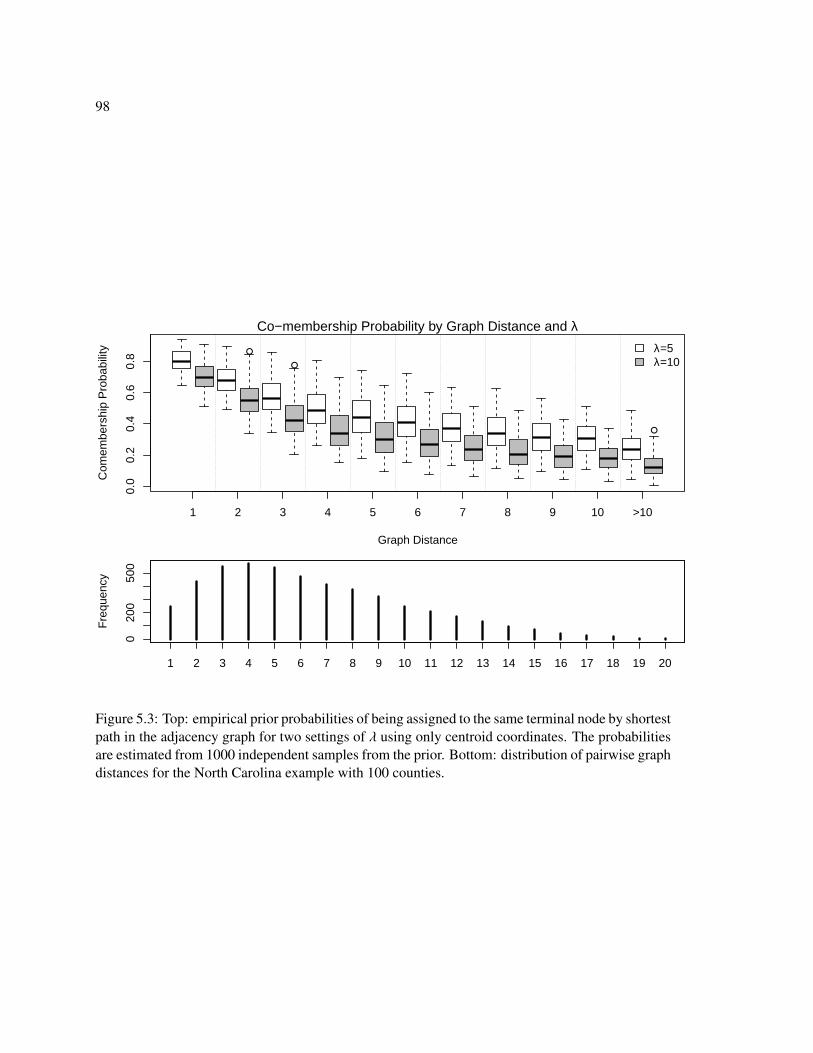
98
●
●
●
Co−membership Probability by Graph Distance and λ
Graph Distance
Com
embe
rshi
p P
roba
bilit
y
1 2 3 4 5 6 7 8 9 10 >10
0.0
0.2
0.4
0.6
0.8
λ=5λ=10
020
050
0
Fre
quen
cy
1 2 3 4 5 6 7 8 9 10 11 12 13 14 15 16 17 18 19 20
Figure 5.3: Top: empirical prior probabilities of being assigned to the same terminal node by shortestpath in the adjacency graph for two settings of λ using only centroid coordinates. The probabilitiesare estimated from 1000 independent samples from the prior. Bottom: distribution of pairwise graphdistances for the North Carolina example with 100 counties.

99
5.5 Combining Trees with Log-linear Models
We analyze sets of spatially referenced multi-way tables by using tree models together with de-
composable log-linear models. The tree splits the observations into groups based on their spatial
features. Conditional on the assignment of observations to the terminal nodes of the tree, the obser-
vations within a given terminal node l share a common log-linear model G(l) and common model
parameters θDG(l) . Thus, within each cluster, the included interactions and the strength of these inter-
actions are identical. The models are independent across nodes, and it is possible to have the same
interactions (i.e., the same graph) for two nodes but different strengths of interactions (i.e., different
values of θ).
For contingency table data, we can simply collapse the contingency tables together to form a sin-
gle table corresponding to each terminal node. If Ll is the list of observations assigned to terminal
node l, then we form (nV )l where
(nV (i))l =∑r∈Ll
(nV (i))r.
Given a particular graph G(l), we obtain the minimal sufficient statistics from the appropriate
marginal counts of (nV )l as described in section 5.2. We call these minimal sufficient statistics
Yl and denote the set of minimal sufficient statistics across all terminal nodes Y. Finally, we denote
the set of graphs and parameters as G and θ. Given this notation, the complete data likelihood for a
tree with L terminal nodes is
p({(nV )r}
Rr=1|{zr}
Rr=1,T,G, θ
)=
L∏l=1
fDG(l)
(Yl; θDG(l)
),
where fDG(l)
(·; θDG(l)
)is defined in (3). Further, the priors on {G, θ} are conditionally independent
given a tree. Thus
π(T,G, θ | α, s) = π(T )π(κT | T )π(τT | T, κT )L∏
l=1
π (G(l)) π(θDG(l) | α, s
).
100
For the remainder of this chapter, we use the DY prior with common α for the log-linear param-
eters at each terminal node, and for the graphs, we assume independent priors that are uniform over
all decomposable graphs. That is π(G) = 1/(# decomposable graphs), which is 1/822 for the 5 way
example in section 5.6 . Note that the only way to find the number of decomposable graphs of a
fixed size is through complete enumeration of graphs, which is difficult if |V | is large. If the number
of nodes is very large, a size-based prior that penalizes larger graphs can be used. For example, Car-
valho and Scott [2009] introduce a hierarchical prior on the edge inclusion probabilities that shrinks
the graph to a “data-determined” size. For the example in section 5.6, we use the pinball prior for T
because of the direct specification of a prior on the number of terminal nodes.
5.5.1 Posterior Inference
The goal of our posterior inference is to estimate the cell probabilities for each area, taking into
account uncertainty in the graphical models and the partitioning implied by the tree structure. We
accomplish this by sampling over the space of trees and graphs and then averaging over the posterior
estimates from each tree-graph model combination in proportion to the marginal probabilities of
these models.
SupposeM1, . . . ,MM is an exhaustive list of models. Each model is defined by a tree and a list
of graphs assigned to the terminal nodes of each treeMk = {T,G}. Then the posterior mean of any
function of the log-linear parameters for the rth county are
g(θr) =
M∑m=1
g(θr(m))Pr(Mm | Y), (5.15)
where g(θr(m)) is the posterior mean for some function of the log-linear parameters for county r under
modelMm and Pr(Mm | Y) is the posterior probability of modelMm. For example, g(θr(m)) could
be the posterior mean of the cell probabilities as given in (5.14), where the data are the contingency
table formed by collapsing over all counties assigned to the same terminal node as county r.
The posterior probability of a given model is proportional to the marginal probability of the data

101
under the model (given in (5.13) for a single table) and the prior for the model:
Pr(Mm | Y) ∝ Pr(Y | Mm)π(Mm), (5.16)
= Pr(Y | T(m),G(m))π(T(m),G(m)), (5.17)
= π(T(m))L(m)∏l=1
Pr(Yl(m)) | Gl(m))π(Gl(m)), (5.18)
where L(m) is the number of terminal nodes of T(m), Yl(m) is the contingency table formed by
collapsing the tables for the counties assigned to terminal node l, and Gl(m) is the graph at terminal
node l under modelMm. Note that many trees can generate the same arrangement of observations at
the terminal nodes, but the prior probability for these trees may differ. The proportionality constant
is the sum of the final expression over all models.
The space of treed graphical models is finite, which means that, in principle, it is possible to
enumerate all models. However, a full enumeration of models is computationally infeasible because
the number of models is extremely large. Instead we explore a subset of the model space with
MCMC and collect a list of models with large posterior probability. Here, we follow the Occam’s
window principal of Madigan and Raftery [1994] and keep a list of models in the set
{Mm :
maxk Pr(Mk | Y)Pr(Mm | Y)
≥ c}
We generate this list by searching over the space of trees and graphs using the Metropolis-Hastings
sampler described below and keep a list models with posterior probabilities that are within c of the
current top model. Chipman et al. [1998, 2002] found that similar samplers do not explore the entire
space of trees, so we run multiple chains from different starting places to better explore the model
space.
5.5.2 Metropolis-Hastings Sampler
We build a list of the models with large posterior probability by sampling the joint posterior of
trees and graphs using the Metropolis-Hastings algorithm. We propose new graphs by perturbing

102
a single edge at a time, and we change the tree by proposing one of four kinds of moves: Swap,
Change, Prune, and Grow. These are the same four moves used in Chipman et al. [1998] and many
subsequent papers relying on the sampler introduced therein. Qualitatively, these moves are
• Swap: swap the splitting rules at a random parent-child pair where both nodes are internal,
• Change: change the splitting rule at a single internal node,
• Grow: split a terminal node into two additional nodes, and
• Prune: merge two terminal nodes with the same parent node into a single terminal node,
The first two moves are standard Metropolis-Hastings moves with transition probabilities
Pr(T→ T′) = min{
1,π(T′ | Y,G)q(T | T′)π(T | Y,G)q(T′ | T)
},
= min{
1,π(T′)Pr(G | T′)Pr(Y | T,G)q(T | T′)π(T)Pr(G | T)Pr(Y | T,G)q(T′ | T)
},
= min
1,π(T′)Pr(Y | T,G)q(T | T′)
π(T)Pr(Y | T,G)q(T′ | T)
,where Y is the data assigned to terminal nodes below the swap or change point. The proposal
probabilities q(T | T′) can be tricky to calculate because some swaps and changes can lead to empty
terminal nodes (which we do not allow), and the number of swappable node pairs or changeable
nodes may differ for T′ and T. In practice we choose uniformly over all internal nodes and then
abort the update if T′ is not a valid tree. If both T and T′ are valid, then the proposals are symmetric.
On the other hand, the grow and prune moves are transdimensional moves: we must propose a
new graph when we split an existing node into two nodes. Suppose we choose to grow a tree by
splitting terminal node u. We generate two new graphs G(2u + 1) and G(2u + 2) by changing a
uniformly-chosen edge in G(u). G(u) can be represented as a binary vector corresponding to the
presence or absence of edges. Let δ be a zero vector of the same length. We choose one element of δ
and set it to −1 or 1 depending on whether the corresponding position in G(u) is 1 or 0. Then we set
{G(2u + 1),G(2u + 2)} = {G(u),G(u) + δ)}. According to Green [1995], the appropriate transition

103
probability for this move is
min
1,Pr
[T′,G(−u),G(2u + 1),G(2u + 2),Y
]pprune(2u + 1, 2u + 2)
Pr(T,G,Y)pgrow(u)p [δ | G(u)]
∣∣∣∣∣∂ {G(2u + 1),G(2u + 2)}∂ {G(u),G(u) + δ)}
∣∣∣∣∣ ,
where the Jacobian here is just 1. Thus the proposal for δ depends on G(u) because only choices of
δ leading to decomposable G(u) + δ are allowed.
Having updated the trees, we update each graph with the same proposal as the graph proposal in
the birth step. We randomly choose an edge and “flip” it, subject to the restriction that the proposed
graph remains decomposable. If the selected edge is missing in the current graph, we add it, and if
the edge is present in the current graph, we delete it. The transition probability for this move is
Pr(G(l)→ G(l)′) =Pr(Y(l) | G(l)′ |nb.dec(G(l))|Pr(Y(l) | G(l) |nb.dec(G(l)′)|
where |nb.dec(G(l))| is the number of decomposable graphs that differ from G(l) by one edge.
Previous authors have observed that the four kinds of tree moves do not efficiently explore the
entire space of trees [Chipman et al., 1998, 2002]. Instead, the Metropolis-Hastings sampler tends to
quickly find a tree of high probability and then explore locally around this tree. To account for this,
previous authors prefer many restarts of short runs of the MCMC over longer runs. Alternatively,
some authors have developed proposals that more drastically change the tree structure to help escape
local modes [Wu et al., 2007, Gramacy and Lee, 2008].
Figure 4 shows that we encounter the same issues when the model space includes both the tree
and the graph. Here we show the unnormalized log posterior probability of the model for the North
Carolina low birthweight data. We show 10 restarts of chains of length 20, 000 compared to a single
chain of length 200, 000. The top models using the restart approach have larger posterior probability
than the models identified from the single, long chain. In addition to using multiple restarts, we use
multiple passes of the graph update step to facilitate joint exploration of the tree space and graph

104
space. Thus, a typical complete iteration t is composed of a single tree transition
Tt → Tt+1,
and 25 updates of the graphs,
Gt+i/25 → Gt+(i+1)/25, i = 0, . . . , 24,
with each update proposing a change to a single graph chosen uniformly from G. Recording the
models at each sub iteration gives a richer list of high probability models.
0 50000 100000 150000 200000
−22
0000
−21
6000
−21
2000
iteration
log
post
erio
r pr
obab
ility
0 50000 100000 150000 200000
−22
0000
−21
6000
−21
2000
iteration
log
post
erio
r pr
obab
ility
Figure 5.4: Unnormalized log posterior probability of the model for 10 restarts of chains of length20, 000 (top) and 1 chain of length 200, 000 (bottom). Restarts are separated by the dashed verticallines. The red line is the maximum value in the top panel.
5.6 Example
In this section, we fit the treed graphical models from section 5.5 to the low birthweight data in-
troduced in section 5.1.2. We compare to a model that incorporates graphical uncertainty with no
105
partitioning of the data and to a model that partitions the data using binary trees but assumes the
graphs are known and complete. We compare these settings using ten fold cross validation. We
split the data into ten bins and form ten data sets–each with one bin held out. We fit our models
and then predict the held out data. Each bin of held out data consists of 100 contingency tables.
In this example, we predict the data assuming that we know the race, sex, maternal smoking, and
full term birth status for the held out data. We predict the low birthweight count for each race, sex,
smoking, and full term birth combination in each of the 100 tables. We compare these predictions
to the observed data based on mean squared error, which is the sum of squared bias and variance.
We estimate the bias and variance by sampling B models in proportion to the posterior probability
of the models and sampling a set of log-linear parameters given each model.
Suppose n∗ is one entry in a held out table andD is the data in the training set. Then the bias is
En∗ |D(n∗ | D
)− n∗ = EM,θ(M)|DEn∗ |M,θ(M),D
(n∗ | M, θ(M),D
)− n∗
≈1B
B∑b=1
E[n∗ | M(b)θ(b)
]− n∗
and the variance is
Varn∗ |D(n∗ | D
)= EM,θ(M)|DVarn∗ |M,θ(M),D
(n∗ | M, θ(M),D
)+ VarM,θ(M)|DEn∗ |M,θ(M),D
(n∗ | M, θ(M),D
)≈
1B
B∑b=1
Var[n∗ | M(b)θ(b)
]+ VarB
(E
[n∗ | M(b)θ(b)
])whereM(b) is sampled in proportion to the posterior probability of the models and θ(b) is sampled
directly from the posterior distribution of the log-linear parameters given the modelM(b) and the
dataD. Here VarB(·) signifies the sample variance based on B samples.
For a given set of log-linear parameters, the expected value E [n∗ | M(b)θ(b)] and variance
Var [n∗ | M(b)θ(b)] are easy to calculate. We transform the log-linear parameters to cell proba-
bilities using (5.2) and calculate the conditional probabilities for each race-sex-smoking-full term

106
combination using the full table of probabilities. Then each missing observation has expected value
n·R,S,SM,F pLBW|R,S,SM,F(b),
and variance
n·R,S,SM,F pLBW|R,S,SM,F(b)(1 − pLBW|R,S,SM,F(b)
),
where n·R,S,SM,F is the marginal count for the race-sex-smoking-full term combination in the held-
out table.
Tables 5.1 and 5.2 show the cross validation results for the 2×2 table formed by low birthweight
and race and the results for the full table of low birthweight, full term birth, race, maternal smoking,
and infant sex. In all cases the prior table total is α = 1 and Occam’s window is c = 1000. For
the treed models, we use the pinball prior with λ = 10 and the tree splits are based on the (x, y)
coordinates of the county centroids. In the 2 × 2 case, fitting models using the treed log-linear
models with complete graphs is superior in terms of MSE. All three models have similar results in
terms of the variance of the predictions, but the bias is substantially smaller when we allow coun-
ties to cluster together. For the full 25 table, however, both models using the tree structure vastly
outperform the model that only takes into account uncertainty in the graphical models. This is not
surprising because there are potentially many more parameters to estimate in the 25 setting than in
the 2 × 2 setting. For counties with small table totals, clustering counties together should be more
beneficial in the 25 case. Again, most of the improvement comes from the spatial partitioning, as
the improvement is modest when the graphs are unknown rather than complete.
Table 5.3 shows the MSE for different specifications of the pinball prior on trees. We investi-
gated different values of λ, which controls the prior number of terminal nodes as well as different
sets of spatial features to split the observations. In addition to the coordinates of the county cen-
troids, we include distance between the centroids and 9 evenly-spaced points (D9) or the distances
between the centroids themselves (D100). The dimensions of z in these three cases is 2, 11, and
102. The centroid+D100 prior has the largest number of possible trees and the greatest potential for

107
MSE BIAS2 VARM = {T,G} 7.37 3.87 3.51M = {G} 14.03 10.37 3.66M = {T} 7.19 3.66 3.53
Table 5.1: MSE results for LBW-RACE.M = {T,G} is our model combining trees with graphicaluncertainty,M = {G} models each county independently and treats the graphs as random,M = {T}uses the spatial partitioning model with fixed, complete graphs.
×10−1 MSE BIAS2 VARM = {T,G} 6.86 3.54 3.32M = {G} 25.46 21.10 4.35M = {T} 6.89 3.52 3.37
Table 5.2: MSE results for full (25) tables. M = {T,G} is our model combining trees with graphicaluncertainty,M = {G} models each county independently and treats the graphs as random,M = {T}uses the spatial partitioning model with fixed, complete graphs.
assigning nonadjacent counties to the same terminal node. In general, the MSE is fairly insensitive
to the choice of λ, and we do see some gains when allowing for disjoint clusters. The best model
is λ = 15 and uses centroids and D100 as spatial features. This suggests that some of the important,
unmeasured risk factors for low birthweight do not have a spatial distribution.
×10−1 (x, y) (x, y) + D9 (x, y) + D100
λ = 5 6.86 6.87 6.84λ = 10 6.86 6.88 6.83λ = 15 6.86 6.86 6.83
Table 5.3: MSE results for 25 models for different tree priors
Now we turn to results of analyzing the complete 25 data with λ = 10 using only the (x, y) coor-
dinates of the centroids. Figure 5.5 shows the prior versus posterior probabilities of comembership
by shortest path in the adjacency graph and the distribution of graph distances. The posterior prob-
ability of co-membership is smaller than the prior probability except for first order neighbors (i.e.,

108
●●●●
●●●●●●●●●●●
●●● ●
●
●●●●
●
●
●
●●●●●●●
●●●●●●●●
●●●
●●●
●●●
●●
●
●●●●●●●●
●
●●●●●
●
●●
●●●●
●●
●●●●
●●
●
●●●●●●
●●●●●
●
●
●
●●●●●●●● ●●
●
●
●
●
●●●●●●●●●
●●
●
●●
●
●●●●●
●
●
●
●●●●●
●●●●●
●
●●
●
●●●●●●●●●●●●●●●●●●●●●●
●●●
●
●
●●
●●●●●●●●●●●●●●
●●●
●
●
●
●
●
●●●●●●●
●
●
●●●●●●●●
●
●●●●●●●●●●●
●
●●●●
●
●●●●●●●●
●
●●●●●
●●
●●
●●
●●●●●●●●●●●●●●●
●
●
●
●●●●●●●●
●●
●
●●
●●
●●●●●
●
●●●●●●●●●
●
●●●●
●●●●
●●●
●
●
●●●●●●●
●●●●
●●●
●
●●●●●●
●●●
●●●
●●
●
●●●●
●●●●●●
●
●
●
●●●●●●●●●●●●●
●
●
●
●
●●●●
●
●
●●●●●●●●●●●●●
●●
●
●●
●
●●●●●
●
●
●
●
●
●●●
●
●●
●●●●●●
●●
●
●
●●●●●●●●●
●●●
●
●●●
●●●●
●●●
●
●●●
●●●●●●●
●
●
●
●●●●●
Prior vs Posterior Comembership by Distance
Graph Distance
Com
embe
rshi
p P
roba
bilit
y
1 2 3 4 5 6 7 8 9 10 >10
0.0
0.4
0.8
priorposterior
030
0
Fre
quen
cy
1 2 3 4 5 6 7 8 9 10 11 12 13 14 15 16 17 18 19 20
Figure 5.5: Prior versus posterior empirical probabilities of comembership based on the shortestpath in the adjacency graph.
adjacent counties). For neighboring areas, the median probability is 0.69 in the prior and 0.83 in
the posterior. For distances 1-7, the distributions of co-membership probabilities covers the whole
range. This means that some neighboring counties are never assigned to the same terminal nodes
and some seventh order neighbors are always assigned to the same terminal nodes. By a distance of
4, the median posterior probability of co-membership is less than 0.1. Thus, the data support many
smaller clusters over a few large clusters. The posterior mean of the number of clusters is 10.
Figure 5.6 shows two possible decomposable log-linear models based on thresholding the pos-
terior probability of including edges, averaged over the 100 counties. We see that most edges have
an average posterior probability of at least 0.5. The two exceptions are also the only two biologically
implausible edges: smoking-sex and race-sex. The model using a cut off of 0.9 has two connected
components and three cliques: [SEX][LBW SMK][LBW RACE FT]. Thus, there is strong evidence
for a three way interaction between low birthweight, full term birth, and race and of a two way
interaction between smoking and low birthweight. The most controversial edges in terms of vari-
ability in posterior inclusion probability between the counties are smoking-full term birth, sex-full

109
LBW
SEX
FT
R
SMK
(a) Average posterior probability > 0.5
LBW
SEX
FT
R
SMK
(b) Average posterior probability > 0.90
Figure 5.6: Graphs based on thresholding the posterior probability of edge inclusion, averaging overthe 100 counties.
term birth, and sex-low birthweight. Figure 5.7 shows the spatial distribution of the posterior mean
for the odds ratio of preterm birth for smokers and non smokers. All odds ratios are greater than 1,
meaning that smokers have greater odds of preterm birth in every county, but the ratios are larger in
western North Carolina.
We do not expect that the effect of smoking is, by itself, more detrimental in western North Car-
olina than in other parts of North Carolina. Instead, there may be other spatially-varying risk factors
that can explain both maternal smoking and poor birth outcomes. For example, the original data
source includes the education level (in years completed) for the mother and the father. Figure 5.8
shows the proportion of white mothers who smoked during pregnancy and the proportion of white
mothers who did not complete high school. We used only white mothers because the vast majority
of births in western North Carolina were to white women. We see a clear similarity in the spatial
patterns of completing high school and smoking during pregnancy. Thus, the spatial heterogeneity
in the smoking-preterm birth effect is at least partially explained by unmeasured confounders (such
as maternal education) that exhibit spatial correlation.
5.7 Discussion
In this chapter, we introduced a new model that accounts for model uncertainty in sets of binary con-
tingency tables generated from distinct spatial locations. In addition to filling a gap in the existing

110
[1,1.2](1.2,1.4](1.4,1.6](1.6,1.8](1.8,2]
Odds Ratios For Pre Term Birth by Smoking
Figure 5.7: Posterior mean for the odds ratio of preterm birth for smokers and non smokers.
[0.021,0.07](0.07,0.12](0.12,0.17](0.17,0.22](0.22,0.27]
Proportion of Mothers not Completing Highschool
[0.018,0.083](0.083,0.15](0.15,0.21](0.21,0.28](0.28,0.35]
Proportion Maternal Smoking
Figure 5.8: Proportion of white mothers who smoked during pregnancy and the proportion of whitemothers who did not complete high school.

111
literature for sets of multi-way contingency tables, the method presented here relies on a partitioning
model that uses a simple, flexible representation of space. While other spatial clustering priors have
been used in the univariate disease mapping literature [Knorr-Held and Raßer, 2000, Green and
Richardson, 2002], these are not as flexible as the tree prior and have some computational draw-
backs compared to the tree approach. For example, the clustering prior in Knorr-Held and Raßer
[2000] only allows for contiguous clusters, and in the Potts model prior in Green and Richardson
[2002], there is always support for noncontiguous clusters. In the treed models, we can impose
contiguous clusters by using only the centroid of the regions, or we can include other features to
allow for noncontiguous clusters.
In this chapter, we restricted our attention to decomposable graphical models because these
graphs have closed-form marginal likelihoods and because we can direct sample the log linear pa-
rameters for these graphs. For the 5-way example in 5.6, the restriction to decomposable graphs
is not very limiting because 80% of 5-node graphs are decomposable. However, as the number of
vertices grows, the fraction of graphical models that are also decomposable decreases [Moghaddam
et al., 2009]. Thus, extending to non-decomposable models using approximations to the marginal
likelihood such as the Laplace approximations in [Dobra and Massam, 2010] will be essential for
examples with more variables.
The combination of treed models and graphical models can easily be extended to other model
selection issues in spatial statistics as long as the marginal likelihood of the data is available in
closed form or via reliable, quick approximations. For example, we can take a similar approach for
common diseases using normal approximations to the binomial or Poisson likelihood to modeling
the logistic or log rate as a linear function of ecological predictors. By using a treed model in this
context, we can include different subsets of demographic summaries or exposure measurements in
the regression models for different parts of the study region.
Finally, the treed approach for multiple contingency tables is also scalable in the number of lo-
cations and naturally accommodates prediction at a new location. Because we collapse to a single
contingency table for each terminal node, the sizes of the tables (i.e. the number of categorical vari-

112
ables) is the major determinant of computation time. For a fixed table size, the computation time for
calculating the marginal likelihood and sampling the table parameters scales linearly in the number
of terminal nodes; whereas, naive implementations of most Bayesian hierarchical models scale (at
best) linearly in the number of observations. Finally, predicting new or missing data is as simple
as finding the corresponding terminal node for the new observation based on the spatial location of
the new data. This can be particularly useful if some locations have only partially observed data.
For example, if some counties do not collect maternal smoking rates, we can fit the treed model to
counties with complete data and impute smoking status for the partially observed counties.
The main weakness of the approach introduced here is our ad hoc stochastic search via mul-
tiple restarts of a Metropolis-Hastings sampler. For simpler model selection problems, algorithms
based on shotgun stochastic search [Hans et al., 2007] or “Occam’s window” [Madigan and Raftery,
1994] systematically search for high probability models. These methods rely on defining a neigh-
borhood of models around a given model. Such neighborhoods are easy to define for graphical
models or subset selection models, but defining and enumerating a neighborhood for a tree is not as
straightforward. Incorporating more drastic tree proposals such as the “restructure” proposal in Wu
et al. [2007] or the “rotate” proposal in Gramacy and Lee [2008] may lead to a more satisfactory
Metropolis-Hastings sampler over the space of trees.

113
Chapter 6
DISCUSSION AND FUTURE WORK
In this thesis, we considered different aspects of analyzing public health data in time or in space.
The development of our methodology was motivated by two examples: cancer incidence data in
Washington State and birth outcome data in North Carolina. In chapter 3 we described a temporal
cancer incidence model and demonstrated how to use this model to forecast incidence for future
years and to estimate the effects of screening rates and tobacco use on female breast cancer and
male lung cancer. In chapter 4 we introduced the negative G-Wishart prior for the covariance ma-
trix of Gaussian spatial random effects. We showed via a simulation study that this new prior has
advantages over the more rigid Gaussian Markov random field (GMRF) priors, and we used this
new prior in a multivariate setting using the cancer incidence data. In chapter 5 we used binary
trees together with graphical log-linear models to capture spatial interactions as well as interactions
between outcomes in sets of spatially dependent binary tables. This approach was illustrated using
the North Carolina data. In this chapter, we present some extensions of our methods and ideas for
future work.
Alternative Flexible Smoothing Models
In chapter 3, we used GMRFs to produce temporally smoothed estimates of cancer screening and
smoking rates to include as covariates in models for cancer incidence. We found that using overly
smoothed estimated led to larger credible intervals for the effects of exposure, and we opted for an
ad hoc way to choose between the smoothed and initial estimates based on sample size. Ideally we
would like to automate the tradeoff in the level of smoothing by using a more flexible prior on the
covariance structure of the temporal random effects. This will be crucial when extending the models
from chapter 3 to include space because there will be fewer observation to estimate each rate and

114
therefore more variability in the initial (unsmoothed) estimates.
One possibility is to use the negative G-Wishart prior from chapter 4, centering on the RW-2 or
perhaps an AR-2 precision matrix for the temporal effects and on the proper CAR for spatial effects.
Alternatively, we propose extending a different proper CAR formulation first introduced by Leroux
et al. [2000]. The Leroux precision matrix for random effects x is the weighted sum of the identity
matrix and an intrinsic GMRF precision matrix:
x ∼ N(0, τ−2
x D−1(λ)),
D(λ) = (1 − λ)I + λQ, for 0 ≤ λ < 1.
The corresponding set of full conditionals is
xi | x−i ∼ N
λ
1 − λ + λni
∑j∈nb(i)
x j,τ2
x
1 − λ + λni
.where ni is the size of the neighborhood of i, and λ is the key parameter to estimate. Lee [2011]
found that the Leroux model adapts to the underlying level of spatial smoothing better than the
intrinsic CAR prior.
We propose extending the basic Leroux model to allow for different weighting parameters for
each random effect. That is, we have a vector λ of the same length as the data instead of a single λ.
Let the unscaled precision of the joint distribution of the random effects be
D(λ) = (1 − Λ)I +√
ΛQ√
Λ,
where Λ is a diagonal matrix of λ. Then the conditional distribution of the random effect for one
area given the rest is
xi | x−i ∼ N
√λi
1 − λi + λini
∑j∈nb(i)
√λ jx j,
τ2x
1 − λi + λini
.

115
If λi is small, then there is less smoothing in the ith random effect. Informative priors can be based
on the sample size (so that there is more support for small λi when the sample size is large), or we
can incorporate a spatial prior on λ so that, a priori, the level of smoothing is similar for adjacent
areas or time points. This model has the advantage of allowing the proportion of variability that is
spatial to vary across the study region.
Sets of Spatially Dependent Tables with Covariates
Ecological measures of socioeconomic factors or exposure to contaminants are often included in
models for birth outcome data like the data in chapter 5. For example, various authors have included
racial segregation, median income, concentrations of particulate matter in the air (PM10 or PM2.5
count), and ozone at the county, zip code, or census tract/block group level [Gray et al., 2010,
Tassone et al., 2010, Anthopolos et al., 2011, Gray et al., 2013]. There are at least two ways to
incorporate covariates into the treed graphical models introduced in chapter 5. First, the covariates
can be included as splitting variables in addition to the spatial features. Under this approach, there
can be different sets of interactions and different log-linear parameters based on the level of the
covariate, but the effect of socioeconomic factors or exposures on the adverse birth outcomes are
difficult to summarize in terms of the usual quantities such as odds ratios.
Alternatively, we can include a regression term on the same scale as the log-linear models. For
example, if D is the the generating set (i.e., a subset of one of the cliques in a graphical model),
θ(D)i = θS (D)i + xTi βD
where θS (D) has the treed graphical model structure and βD is a vector of regression parameters
specific to the D log-linear parameters. This is similar to the spatial log-linear model of Tassone
et al. [2010], who use intrinsic CAR priors for the spatial portion and a different parameterization
of the log-linear model.
The regression parameters can be interpreted as changes in log odds ratios, where the exact odds

116
being compared depend on D (see equation 5.4). For example, if D = {LBW}, then
θ(D)i = θS (D)i + xTi βD = log
p(LBW = 2,FT = 1,RACE = 1,SMK = 1,SEX = 1 | xi)p(LBW = 1,FT = 1,RACE = 1,SMK = 1,SEX = 1 | xi)
.
Thus, βD is the change in the log odds of low birthweight associated with a one unit increase in the
covariate within the FT = 1,RACE = 1,SMK = 1,SEX = 1 group.
While the effect of the covariates are easier to interpret with this approach, there are several
computational and practical challenges. First, the computation for the treed models relies on direct
calculation (or at least a quick, reliable approximation) of the marginal likelihood of the data given
a graphical model. It is not initially apparent that this is possible with the addition of the regression
terms. Second, the dimension of the vector of log-linear parameters changes with the graphical
model, and the regression terms should only be included when the corresponding log-linear param-
eter is included. One solution is to only include the regression terms for main effects (|D| = 1),
which are always included.
In this thesis, we strove to develop flexible and scientifically plausible spatial and temporal mod-
els to answer key public health questions. As the availability of detailed information on individual-
level risk factors and health outcomes increases and as computational methods rise to meet the
challenges of analyzing these rich data sets, the tools and ideas we have presented will continue to
help us understand and treat diseases.

117
BIBLIOGRAPHY
A. Agresti. Categorical Data Analysis. Wiley, 1990.
G.R. Alexander, M.D. Kogan, and J. H. Himes. 1994–1996 US singleton birth weight percentiles
for gestational age by race, Hispanic origin, and gender. Maternal and Child Health Journal, 3
(4):225–231, 1999.
R. Anthopolos, S.A. James, A.E. Gelfand, and M.L. Miranda. A spatial measure of neighborhood
level racial isolation applied to low birthweight, preterm birth, and birthweight in North Carolina.
Spatial and spatio-temporal epidemiology, 2(4):235–246, 2011.
A. Atay-Kayis and H. Massam. A Monte Carlo method for computing the marginal likelihood in
nondecomposable Gaussian graphical models. Biometrika, 92:317–335, 2005.
S. Banerjee, B.P. Carlin, and A.E. Gelfand. Hierarchical Modeling and Analysis for Spatial Data,
volume 101. Chapman & Hall, 2004.
C. Berzuini and D. Clayton. Bayesian analysis of survival on multiple time scales. Statistics in
medicine, 13(8):823–838, 1994.
J. Besag. Spatial interaction and the statistical analysis of lattice systems. Journal of the Royal
Statistical Society: Series B (Methodological), pages 192–236, 1974.
J. Besag and C. Kooperberg. On conditional and intrinsic autogregressions. Biometrika, 82:733–
746, 1995.
J. Besag, J. York, and A. Mollie. Bayesian image restoration, with two applications in spatial
statistics. Annals of the Institute of Statistical Mathematics, 1991.
J. Besag, P. Green, D. Higdon, and K. Mengersen. Bayesian computation and stochastic systems.
Statistical Science, pages 3–41, 1995.

118
Y.M.M. Bishop, S.E. Fienberg, and P.W. Holland. Discrete Multivariate Analysis: Theory and
Practice. M.I.T. Press, 1975. Cambridge, MA.
P. Bremaud. Markov chains: Gibbs fields, Monte Carlo simulation, and queues. Springer, 1999.
Cancer Research UK. Cancer statistics by type. http://www.cancerresearchuk.org/
cancer-info/cancerstats/types/, 2013. Last visited on 01/05/2013.
B. Carstensen. Age–period–cohort models for the lexis diagram. Statistics in medicine, 26(15):
3018–3045, 2007.
C.M. Carvalho and J.G. Scott. Objective Bayesian model selection in Gaussian graphical models.
Biometrika, 96(3):497–512, 2009.
C.M. Carvalho and M. West. Dynamic matrix-variate graphical models. Bayesian Analysis, 2(1):
69–97, 2007.
J. Challis, J. Newnham, F. Petraglia, M. Yeganegi, and A. Bocking. Fetal sex and preterm birth.
Placenta, 34(2):95–99, 2013.
M.H.. Chen, Q. Shao, and J.G. Ibrahim. Monte Carlo Methods in Bayesian Computation. Springer
New York, 2000.
H.A. Chipman, E.I. George, and R.E. McCulloch. Bayesian CART model search. Journal of the
American Statistical Association, 93(443):935–948, 1998.
H.A. Chipman, E.I. George, and R.E. McCulloch. Bayesian treed models. Machine Learning, 48
(1-3):299–320, 2002.
H.A. Chipman, E.I. George, and R.E. McCulloch. Bart: Bayesian additive regression trees. The
Annals of Applied Statistics, 4(1):266–298, 2010.
D. Clayton and E. Schifflers. Models for temporal variation in cancer rates. I: age–period and age–
cohort models. Statistics in medicine, 6(4):449–467, 1987a.

119
D. Clayton and E. Schifflers. Models for temporal variation in cancer rates. II: age–period–cohort
models. Statistics in medicine, 6(4):469–481, 1987b.
C.C. Clogg and L.A. Goodman. Latent structure analysis of a set of multidimensional contingency
tables. Journal of the American Statistical Association, pages 762–771, 1984.
A.P. Dawid. Some matrix-variate distribution theory: notational considerations and a Bayesian
application. Biometrika, 68:265–274, 1981.
A.P. Dawid and S. L. Lauritzen. Hyper markov laws in the statistical analysis of decomposable
graphical models. The Annals of Statistics, pages 1272–1317, 1993.
A.P. Dempster. Covariance selection. Biometrics, pages 157–175, 1972.
P. Diaconis and D. Ylvisaker. Conjugate priors for exponential families. Annals of Statisstics, 7:
269–281, 1979.
P. Diggle, B. Rowlingson, and T. Su. Point process methodology for on-line spatio-temporal disease
surveillance. Environmetrics, 16(5):423–434, 2005.
P.J. Diggle, J.A. Tawn, and R.A. Moyeed. Model-based geostatistics. Journal of the Royal Statistical
Society: Series C (Applied Statistics), 47:299–350, 1998.
P.J. Diggle, P. Moraga, B. Rowlingson, and B.P. Taylor. Spatial and spatio-temporal log-Gaussian
Cox processes: Extending the geostatistical paradigm. Statistical Science, 28(4):542–563, 2013.
A. Dobra and H. Massam. The mode oriented stochastic search (MOSS) algorithm for log-linear
models with conjugate priors. Statistical Methodology, 7(3):240–253, 2010.
A. Dobra, A. Lenkoski, and A. Rodriguez. Bayesian inference for general Gaussian graphical mod-
els with applications to multivariate lattice data. Journal of the American Statistical Association,
2011.
J. Escedy and D. Hunter. The origin of cancer. In H. O. Adami, D. Hunter, and D. Trichopoulos,
editors, Textbook of Cancer Epidemiology. Oxford University Press, 2 edition, 2008.

120
J.M. Flegal and G.L. Jones. Implementing MCMC: estimating with confidence. Handbook of
Markov chain Monte Carlo, Boca Raton, Florida: Chapman & Hall/CRC, pages 175–197, 2011.
Y. Fong, H. Rue, and J. Wakefield. Bayesian inference for generalized linear mixed models. Bio-
statistics, 11(3):397–412, 2010.
N.D. Freedman, M.F. Leitzmann, A.R. Hollenbeck, A. Schatzkin, and C.C. Abnet. Cigarette smok-
ing and subsequent risk of lung cancer in men and women: analysis of a prospective cohort study.
The lancet oncology, 9(7):649–656, 2008.
D. Gamerman. Dynamic spatial models including spatial time series. Handbook of Spatial Statistics,
pages 437–448, 2010.
A.E. Gelfand and P. Vounatsou. Proper multivariate conditional autoregressive models for spatial
data analysis. Biostatistics, 4:11–15, 2003.
K. Ghosh and R.C. Tiwari. Prediction of US cancer mortality counts using semiparametric Bayesian
techniques. Journal of the American Statistical Association, 102(477):7–15, 2007.
K. Ghosh, R.C. Tiwari, E.J. Feuer, K. Cronin, and A. Jemal. Predicting US cancer mortality counts
using state space models. Computational Methods in Biomedical Research, Eds. R. Khattree &
DN Naik, pages 131–151, 2007.
T. Gneiting and P. Guttorp. Continuous parameter spatio-temporal processes. Handbook of Spatial
Statistics, 97:427–436, 2010.
L.A. Goodman. Guided and unguided methods for the selection of models for a set of t multidi-
mensional contingency tables. Journal of the American Statistical Association, pages 165–175,
1973.
L.A. Goodman. Exploratory latent structure analysis using both identifiable and unidentifiable mod-
els. Biometrika, 61(2):215–231, 1974.

121
R.B. Gramacy and K.H. Lee. Bayesian treed Gaussian process models with an application to com-
puter modeling. Journal of the American Statistical Association, 103(483), 2008.
S.C. Gray, S.E. Edwards, and M.L. Miranda. Assessing exposure metrics for PM and birth weight
models. Journal of Exposure Science and Environmental Epidemiology, 20(5):469–477, 2010.
S.C. Gray, S.E. Edwards, and M.L. Miranda. Race, socioeconomic status, and air pollution exposure
in North Carolina. Environmental research, 2013.
P. J. Green and S. Richardson. Hidden Markov models and disease mapping. Journal of the Ameri-
can Statistical Association, 97:1055–1070, 2002.
P.J. Green. Reversible jump Markov chain Monte Carlo computation and Bayesian model determi-
nation. Biometrika, 82(4):711–732, 1995.
S. Haneuse and J. Wakefield. Ecological inference incorporating spatial dependence. In G. King,
O. Rosen, and M. Tanner, editors, Ecological inference: new methodological strategies, chap-
ter 12, pages 266–301. Cambridge University Press, 2004.
C. Hans, A. Dobra, and M. West. Shotgun stochastic search for large p regression. Journal of the
American Statistical Association, 102(478):507–516, 2007.
W.K. Hastings. Monte Carlo sampling methods using Markov chains and their applications.
Biometrika, 57(1):97–109, 1970.
L. Held, B. Schrodle, and H. Rue. Posterior and cross-validatory predictive checks: a comparison of
MCMC and INLA. In Statistical Modelling and Regression Structures, pages 91–110. Springer,
2010.
S.J. Henley, C.R. Ehemen, L.C. Richarsdon, M. Plescia, K.J. Asman, S.R. Dube, R.S. Carballo,
and T.A. McAfee. State-specific trends in lung cancer incidence and smoking–United States,
1999-2008. Morbidity and mortality weekly report (MMWR), 60(36):1243–1247, 2011.

122
C. Heuer. Modeling of time trends and interactions in vital rates using restricted regression splines.
Biometrics, pages 161–177, 1997.
D.G. Horvitz and D.J. Thompson. A generalization of sampling without replacement from a finite
universe. Journal of the American Statistical Association, 47(260):663–685, 1952.
J. Hughes and M. Haran. Dimension reduction and alleviation of confounding for spatial generalized
linear mixed models. Journal of the Royal Statistical Society: Series B (Statistical Methodology),
75:139–159, 2013.
D. Ingram, J. Parker, N. Schenker, J. Weed, B. Hamilton, E. Arias, and J. Madans. United States
Census 2000 population with bridged race categories. Vital and Helath Statistics, 2(134), Septem-
ber 2003.
C. Jackson, N. Best, and S. Richardson. Hierarchical related regression for combining aggregate and
individual data in studies of socio-economic disease risk factors. Journal of the Royal Statistical
Society: Series A (Statistics in Society), 171(1):159–178, 2008.
X. Jin, S. Banerjee, and B.P. Carlin. Order-free co-regionalized areal data models with applica-
tion to multiple-disease mapping. Journal of the Royal Statistical Society: Series B (Statistical
Methodology), 69:817–838, 2007.
L. Knorr-Held. Bayesian modelling of inseparable space-time variation in disease risk. Statistics in
Medicine, 19(17-18):2555–2567, 2000.
L. Knorr-Held and N. Best. A shared component model for detecting joint and selective clustering
of two diseases. Journal of the Royal Statistical Society: Series A (Statistics in Society), 164,
2001.
L. Knorr-Held and E. Rainer. Projections of lung cancer mortality in West Germany: a case study
in Bayesian prediction. Biostatistics, 2(1):109–129, 2001.
L. Knorr-Held and G. Raßer. Bayesian detection of clusters and discontinuities in disease maps.
Biometrics, pages 13–21, 2000.

123
D. Kuang, B. Nielsen, and J.P. Nielsen. Forecasting with the age-period-cohort model and the
extended chain-ladder model. Biometrika, 95(4):987–991, 2008a.
D. Kuang, B. Nielsen, and J.P. Nielsen. Identification of the age-period-cohort model and the ex-
tended chain-ladder model. Biometrika, 95(4):979–986, 2008b.
C. Lagazio, A. Biggeri, and E. Dreassi. Age–period–cohort models and disease mapping. Environ-
metrics, 14(5):475–490, 2003.
S.L. Lauritzen. Graphical Models. Clarendon Press, Oxford, 1996.
D. Lee. A comparison of conditional autoregressive models used in Bayesian disease mapping.
Spatial and Spatio-temporal Epidemiology, 2(2):79–89, 2011.
D. Lee, A. Rushworth, and S. Sahu. A Bayesian localised conditional auto-regressive model for
estimating the health effects of air pollution. Biometrics, 2014.
B.G. Leroux, X. Lei, and N. Breslow. Estimation of disease rates in small areas: A new mixed model
for spatial dependence. In Statistical Models in Epidemiology, the Environment, and Clinical
Trials, pages 179–191. Springer, 2000.
T. Lumley. Complex surveys: A guide to analysis using R. John Wiley & Sons, 2011.
D. Madigan and A.E. Raftery. Model selection and accounting for model uncertainty in graphical
models using Occam’s window. Journal of the American Statistical Association, 89(428):1535–
1546, 1994.
H. Massam, J. Liu, and A. Dobra. A conjugate prior for discrete hierarchical log-linear models.
Annals of Statistics, 37:3431–3467, 2009.
L. Mercer, J. Wakefield, C. Chen, and T. Lumley. A comparison of spatial smoothing methods for
small area estimation with sampling weights. Spatial Statistics, 2013.
N. Metropolis, A.W. Rosenbluth, M.N. Rosenbluth, A.H. Teller, and Teller E. Equations of state
calculations by fast computing machines. Journal of Chemical Physics, 21(1087):L7, 1953.

124
M.D.M. Miranda, B. Nielsen, and J.P. Nielsen. Inference and forecasting in the age–period–cohort
model with unknown exposure with an application to mesothelioma mortality. Journal of the
Royal Statistical Society: Series A (Statistics in Society), 2014.
B. Moghaddam, B.M. Marlin, M.E. Khan, and K.P. Murphy. Accelerating Bayesian structural
inference for non-decomposable Gaussian graphical models. In NIPS, pages 1285–1293, 2009.
P.A.P. Moran. Notes on continuous stochastic phenomena. Biometrika, 37(1-2):17–23, 1950.
S. Murin, R. Rafii, and K. Bilello. Smoking and smoking cessation in pregnancy. Clinics in Chest
Medicine, 32(1):75–91, 2011.
B. Nielson and J.P. Nielsen. Identification and forcasting in mortality models. January 2014.
F.F. Nobre, A. Monteiro, P.R. Telles, and G.D. Williamson. Dynamic linear model and SARIMA:
a comparison of their forecasting performance in epidemiology. Statistics in medicine, 20(20):
3051–3069, 2001.
C. J. Paciorek. The importance of scale for spatial-confounding bias and precision of spatial regres-
sion estimators. Statistical science: a review journal of the Institute of Mathematical Statistics,
25(1):107, 2010.
L.I. Pettit. The conditional predictive ordinate for the normal distribution. Journal of the Royal
Statistical Society. Series B (Methodological), pages 175–184, 1990.
M. Plummer. Penalized loss functions for Bayesian model comparison. Biostatistics, 9(3):523–539,
2008.
R. Prado and M. West. Time series: modeling, computation, and inference. CRC Press, 2010.
H. Quick, S. Banerjee, B.P. Carlin, et al. Modeling temporal gradients in regionally aggregated
California asthma hospitalization data. The Annals of Applied Statistics, 7(1):154–176, 2013.
B.J. Reich, J.S. Hodges, and V. Zadnik. Effects of residual smoothing on the posterior of the fixed
effects in disease-mapping models. Biometrics, 62(4):1197–1206, 2006.

125
A. Riebler, L. Held, and H. Rue. Estimation and extrapolation of time trends in registry data–
borrowing strength from related populations. The Annals of Applied Statistics, 6(1):304–333,
2012.
A. Roverato. Hyper inverse Wishart distribution for non-decomposable graphs and its application
to Bayesian inference for Gaussian graphical models. Scandinavian Journal of Statistics, 29:
391–411, 2002.
H. Rue and L. Held. Gaussian Markov Random Fields, volume 104 of Monographs on Statistics
and Applied Probability. Chapman & Hall/CRC, Boca Raton, FL, 2005.
H. Rue, S. Martino, and N. Chopin. Approximate Bayesian inference for latent Gaussian models by
using integrated nested Laplace approximations. Journal of the Royal Statistical Society: Series
B (Statistical Methodology), 71:319–392, 2009.
D.J. Spiegelhalter, N.G. Best, B.P. Carlin, and A. Van Der Linde. Bayesian measures of model
complexity and fit. Journal of the Royal Statistical Society: Series B (Statistical Methodology),
64(4):583–639, 2002.
State Center for Health Statisticss (NC SCHS). North Carolina vital statistics – births 2006, 2007.
URL http://hdl.handle.net/1902.29/10130. Distributed by the Odem Institute for Re-
search in Social Science.
E.C. Tassone, M.L. Miranda, and A.E. Gelfand. Disaggregated spatial modelling for areal unit
categorical data. Journal of the Royal Statistical Society: Series C (Applied Statistics), 59(1):
175–190, 2010.
United States Department of Health and Human Services, Centers for Disease Control and Preven-
tion, National Center for Health Statistics (NCHS). Bridged-race population estimates, United
States July 1st resident population by state, county, age, sex, bridged-race, and Hispanic ori-
gin. Compiled from 1990-1999 bridged-race intercensal population estimates (released by NCHS
on 7/26/2004); revised bridged-race 2000-2009 intercensal population estimates (released by

126
NCHS on 10/26/2012); and bridged-race vintage 2011 (2010-2011) postcensal population es-
timates (released by NCHS on” ”7/18/2012).. Available on CDC WONDER on-line database.
http://wonder.cdc.gov/bridged-race-v2011.html, 2012. Last visited on 23/02/2014.
J. Wakefield. Ecological inference for 2×2 tables (with discussion). Journal of the Royal Statistical
Society: Series A (Statistics in Society), 167(3):385–445, 2004.
J. Wakefield. Disease mapping and spatial regression with count data. Biostatistics, 8(2):158–183,
2007.
J. Wakefield and H. Lyons. Spatial aggregation and the ecological fallacy. In A.E. Gelfand, P. Diggle,
P. Guttorp, and M. Fuentes, editors, Handbook of Spatial Statistics. CRC Press, 2010.
J. Wakefield, S. Haneuse, A. Dobra, and E. Teeple. Bayes computation for ecological inference.
Statistics in Medicine, 2011.
M.M. Wall. A close look at the spatial structure implied by the CAR and SAR models. Journal of
Statistical Planning and Inference, 121:311–324, 2004.
M.M. Wall and X. Liu. Spatial latent class analysis model for spatially distributed multivariate
binary data. Computational statistics & data analysis, 53(8):3057–3069, 2009.
H. Wang and N.S. Pillai. On a class of shrinkage priors for covariance matrix estimation. Journal
of Computational and Graphical Statistics, To appear, 2013.
H. Wang and M. West. Bayesian analysis of matrix normal graphical models. Biometrika, 96(4):
821–834, 2009.
Washington State Department of Health, Center for Health Statistics, Behavioral Risk Factor
Surveillance Systems (WA CHS). supported in part by Centers for Disease Control and Preven-
tion, Cooperative Agreement U58/CCU002118- 6 through 17 (1992-2003), U58/CCU022819-1
through 5 (2004-2008), and U58 DP001996-1 through 2 (2009-2010), 2010.
M. West and J. Harrison. Bayesian Forecasting and Dynamic Models. Springer, 2nd edition, 1997.

127
G. White and S.K. Ghosh. A stochastic neighborhood conditional autoregressive model for spatial
data. Computational Statistics & Data Analysis, 53:3033–3046, 2009.
T.J. Wilkin and M.J. Murphy. The gender insulin hypothesis: why girls are born lighter than boys,
and the implications for insulin resistance. International journal of obesity, 30(7):1056–1061,
2006.
J. Windle, N.G. Polson, and J.G. Scott. Sampling polya-gamma random variates: alternate and
approximate techniques. arXiv preprint arXiv:1405.0506, 2014.
Y. Wu, H. Tjelmeland, and M. West. Bayesian CART: Prior specification and posterior simulation.
Journal of Computational and Graphical Statistics, 16(1):44–66, 2007.
J. Zeitlin, M. Saurel-Cubizolles, J.S. de Mouzon, L. Rivera, P. Ancel, B. Blondel, and M. Kaminski.
Fetal sex and preterm birth: are males at greater risk? Human Reproduction, 17(10):2762–2768,
2002.
L. Zhu, L.W. Pickle, K. Ghosh, D. Naishadham, K. Portier, H. Chen, H. Kim, J. Zou, Z. Cucinelli,
B. Kohler, B.K. Edwards, J. King, E.J. Feuer, and A. Jemal. Predicting US-and state-level cancer
counts for the current calendar year. Cancer, 118(4):1100–1109, 2012.
L. Zhu, L. W. Pickle, Z. Zou, and J. Cucinelli. Trends and patterns of childhood cancer incidence in
the United States, 1995-2010. Statistics and Its Iterface, pages 1–14, 2013.

128
Appendix A
SUPPLEMENT TO CHAPTER 3
A.1 INLA versus MCMC
We fit the AP model for breast cancer and the AC model for lung cancer in using MCMC with Win-
BUGs and with INLA. We use the car.normal prior built into WinBUGS for the RW-2 effects. The
figures and tables below compare the point estimates of the overall log rate and variance components
and for the random effects for these model. The MCMC estimates are based on 500,000 iterations,
saving every 50th iteration This takes approximately 15 minutes in WinBUGS (compared to 3 sec-
onds with INLA). The overall means and random effects match, but there are some differences in
the estimates of the variances of the random effects.
MCMC(BUGS) INLAδ -6.106 -6.106
σα 0.179 0.187σβ 0.0135 0.0157σz 0.0709 0.0703
Table A.1: Comparison of posterior medians for the breast AP model.
MCMC(BUGS) INLAδ -7.557 -7.543
σα 0.138 0.137σγ 0.00775 0.00834σz 0.0379 0.0377
Table A.2: Comparison of posterior medians for the lung AC model.
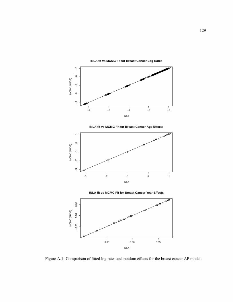
129
●●●●● ●●●●●●●●●●● ●●●
●● ●●●●
●●●●●●●●
●●●●●
●●●●●●●
●●●●●●●●●●●●
●●●●●●●●●●●●●●●●●●●
●● ●●●
●●●●●●●●●●●● ●●●●●●●●●●●●
●●●●●●●●●
●●●●●●●●●●●●●●
●●●●●
●●● ●●
●●●●●●
●●●●●
●●● ● ●●●●●●●●●●
●●●● ●●●●●●●●● ●●●●●●●●●●●
●●●●●●●●●
●●●●●●●●● ●●
●●
●●●●●●●●●●●
●●●●● ●
●●
●●●●
●●●●●●
●●
●●●●●●●
−9 −8 −7 −6 −5
−9
−8
−7
−6
−5
INLA fit vs MCMC Fit for Breast Cancer Log Rates
INLA
MC
MC
(B
UG
S)
●
●
●
●
●●
●●
● ●●●
●
−3 −2 −1 0 1
−3
−2
−1
01
INLA fit vs MCMC Fit for Breast Cancer Age Effects
INLA
MC
MC
(B
UG
S)
●
●
●
●
●
●
●
●●●
●
●
●
●
●●
●
●●
−0.05 0.00 0.05
−0.
050.
000.
05
INLA fit vs MCMC Fit for Breast Cancer Year Effects
INLA
MC
MC
(B
UG
S)
Figure A.1: Comparison of fitted log rates and random effects for the breast cancer AP model.

130
●●●●●●●●●●●●●●●●●●●
●●●●●●●●●●●●●●●●●●●
●●●●●●●●●●●●●●●●●●●
●●●●●●●●●●●●●●●●●●●
●●●●●●●●●●●●●●●●●●●
●●●●●●●●●●●●●●●●●●●
●●●●●●●●●●●●●●●●●●●
●●●●●●●●●●●●●●●●●●●
●●●●●●●●●●●●●●●●●●●
●●●●●●●●●●●●●●●●●●●●●●●●●●●●●●●●●●●●●●●●●●●●●●●●●●●●●●●●●
●●●●●●●●●●●●●●●●●●●
−12 −10 −8 −6
−12
−10
−8
−6
INLA fit vs MCMC Fit for Lung Cancer Log Rates
INLA
MC
MC
(B
UG
S)
●
●
●
●
●
●
●
●●
●●●●
−3 −2 −1 0 1
−4
−3
−2
−1
01
INLA fit vs MCMC Fit for Lung Cancer Age Effects
INLA
MC
MC
(B
UG
S)
●●●●●●●●●●●●
●●●●●●●●●●●●●●●●●●●●●●
●●
●●
●●
●●●●●●●●●●●●●●●●●
●●
●●
●●
●●
●●
●●
●●
●●
●●●●
●●
−1.0 −0.5 0.0 0.5
−1.
0−
0.5
0.0
0.5
INLA fit vs MCMC Fit for Lung Cancer Cohort Effects
INLA
MC
MC
(B
UG
S)
Figure A.2: Comparison of fitted log rates and random effects for the breast cancer AP model.

131
A.2 Forecasts
Figure A.3 shows the posterior means of the forecasts of the 2010 counts from the four different
models from section 3.4 versus the observed count. The next several pages (Figure A.4 – A.9) show
projected incidence for 2011–2015 based on observing 1992–2010. We show the posterior mean for
the each year as well as 80% point wise posterior predictive intervals. We use population projections
from the Washington State Office of Financial Management (November, 2013).
We MCMC output to approximate the posterior distributions of the forecasted counts. That is,
for each iteration b we have
ybi,T+h ∼ Poi(Ni,T+h exp(δb + αb
i + βbT+h + γb
k(i,T )+h + zbi,T+h)).
The δ and αi terms are already in the MCMC, and we assume Ni,T+h is fixed and known. The
unstructured random effects are sampled independently from N(0, (τ−2z )b). There are two ways to
generate the period and cohort effects. Using the suggestion of Kuang et al. [2008a], we simulate
βT+h ∼ N(βb
T + hsbβ, h(σ2
∆β)b),
where sbβ is defined in equation 3.2 and (σ2
∆β)b is the sample variance of the first differences. Alter-
natively, we can generate from the RW-2 model [Rue and Held, 2005]:
βT+h | β1:T ∼ N
βbT + h∆βb
T ,1 + 22 + · · · + h2
(τ2β)
b
.For Figure A.3 and for the MSE comparisons of the four models in section 3.4, we only use the
Kuang et al. [2008a] projections. For the 2011–2015 forecasts, we use both forecasting methods.
The choice matters very little for the cohort effects because the we only forecast cohort effects for
the first age group. For the breast cancer data, the projected period effects are slightly smaller when
generating from the RW-2 model. We project an average of five fewer cases per age band and year
with the RW-2 model.

132
●
●
●
●
●
●
● ●
●
●
●
●
●
0 200 400 600 800 1000
020
040
060
080
010
00
Breast Cancer Observed versus Predicted, 2010
Observed
Pre
dict
ed (
Pos
terio
r M
ean)
●●
●
●
●
●
● ●
●
●
●
●
●
●●
●
●
●
●
●●
●
●
●
●
●
●●
●
●
●
●
●●
●
●
●
●
●
●
●
●
●
AAPACAPC
●●●●
●
●
●
●
●●
●
●
●
0 100 200 300 400
010
020
030
040
0
Lung Cancer Observed versus Predicted, 2010
Observed
Pre
dict
ed (
Pos
terio
r M
ean)
●●●
●
●
●
●
●
●
●
●
●
●
●●●
●
●
●
●
●
●
●
●
●
●
●●●●
●
●
●
●
●●
●
●
●
●
●
●
●
AAPACAPC
Figure A.3: Forecasts versus observed values for the four APC models for breast and lung cancer.
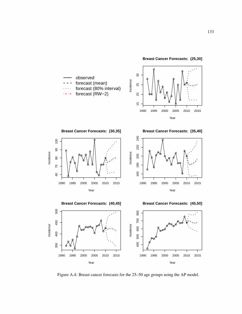
133
observedforecast (mean)forecast (80% interval)forecast (RW−2)
1990 1995 2000 2005 2010 2015
1520
2530
Breast Cancer Forecasts: (25,30]
Year
Inci
denc
e ●
● ●
●
●
●
●
●
●
●
●
●
●
●
●
●
●
●●
1990 1995 2000 2005 2010 2015
6070
8090
100
Breast Cancer Forecasts: (30,35]
Year
Inci
denc
e
●
●
●
●
●
●
● ●
●
●
●
●
●
●
●
●
● ●
●
1990 1995 2000 2005 2010 2015
160
180
200
220
240
Breast Cancer Forecasts: (35,40]
Year
Inci
denc
e
●
●
●
●
●
●●
●
●
●
●
●
●
●
● ●
●
●
●
1990 1995 2000 2005 2010 2015
350
400
450
500
Breast Cancer Forecasts: (40,45]
Year
Inci
denc
e
●
●
●
●
●
●
●
● ●
● ● ●●
●
●●
●
●
●
1990 1995 2000 2005 2010 2015
400
500
600
700
800
Breast Cancer Forecasts: (45,50]
Year
Inci
denc
e
●
●
● ●●
●
● ● ●
●● ●
●●
●● ●
●
●
Figure A.4: Breast cancer forecasts for the 25–50 age groups using the AP model.
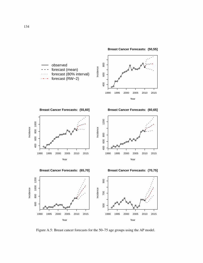
134
observedforecast (mean)forecast (80% interval)forecast (RW−2)
1990 1995 2000 2005 2010 2015
400
600
800
Breast Cancer Forecasts: (50,55]
YearIn
cide
nce
● ●
● ●
●
●
●●
●●
●
●
●● ●
●
●
●
●
1990 1995 2000 2005 2010 2015
400
600
800
1000
Breast Cancer Forecasts: (55,60]
Year
Inci
denc
e
●●
● ●●
●
●● ●
● ● ● ●
●●
●
●
●●
1990 1995 2000 2005 2010 2015
400
600
800
1200
Breast Cancer Forecasts: (60,65]
Year
Inci
denc
e
●●
●●
●
● ●●
● ●
●
●●
●
●●
●●
●
1990 1995 2000 2005 2010 2015
600
800
1000
1200
Breast Cancer Forecasts: (65,70]
Year
Inci
denc
e
●●
●● ● ●
●●
● ● ●
● ●● ●
●
●
● ●
1990 1995 2000 2005 2010 2015
500
700
900
Breast Cancer Forecasts: (70,75]
Year
Inci
denc
e
●●
●●
●
●
●
●
●●
●
●
●
●
●●
● ●●
Figure A.5: Breast cancer forecasts for the 50–75 age groups using the AP model.

135
observedforecast (mean)forecast (80% interval)forecast (RW−2)
1990 1995 2000 2005 2010 201535
045
055
0
Breast Cancer Forecasts: (75,80]
Year
Inci
denc
e●
●
● ●
●
●
●
●
● ●
●
●
●●
●
● ●
●
●
1990 1995 2000 2005 2010 2015
250
300
350
400
Breast Cancer Forecasts: (80,85]
Year
Inci
denc
e
●
●
●●
●
●●
●
●
●
●
●
●
●
●
●
●
●
●
1990 1995 2000 2005 2010 2015
150
200
250
300
350
Breast Cancer Forecasts: (85,110]
Year
Inci
denc
e
●●
●
●
●
●
●
●
●
●
●
●
● ● ●
●
●
●
●
Figure A.6: Breast cancer forecasts for the 75+ age groups using the AP model.

136
observedforecast (mean)forecast (80% interval)forecast (RW−2)
1990 1995 2000 2005 2010 2015
01
23
Lung Cancer Forecasts: (25,30]
YearIn
cide
nce
●
●
●
●
● ● ●
● ●
●
●
● ●
●
●
●
●
●
●
1990 1995 2000 2005 2010 2015
12
34
56
Lung Cancer Forecasts: (30,35]
Year
Inci
denc
e
●
●
●
●
●
●
●
● ● ● ●
● ●
●
●
●
●
● ●
1990 1995 2000 2005 2010 2015
510
15
Lung Cancer Forecasts: (35,40]
Year
Inci
denc
e
●
●
●
●
●
●
●
●
●
●
●
●
●
●
●
●
●
●
●
1990 1995 2000 2005 2010 2015
1520
2530
3540
Lung Cancer Forecasts: (40,45]
Year
Inci
denc
e
●
●
●
●
●●
●●
●
●
●
●
●
●
●
● ●
●
●
1990 1995 2000 2005 2010 2015
4050
6070
8090
Lung Cancer Forecasts: (45,50]
Year
Inci
denc
e
●
●
● ● ●
●
●
●
● ●●
●
●
●
●
●
●
●●
Figure A.7: Lung cancer forecasts for the 25–50 age groups using the AC model.

137
observedforecast (mean)forecast (80% interval)forecast (RW−2)
1990 1995 2000 2005 2010 2015
100
120
140
Lung Cancer Forecasts: (50,55]
Year
Inci
denc
e
●
●
●●
●
● ●
●
●
●
● ●
●
●
●
●
●
●
●
1990 1995 2000 2005 2010 2015
180
200
220
240
Lung Cancer Forecasts: (55,60]
Year
Inci
denc
e
●
●
●
●
●
●
●
●
●
●
●
●●
●●
●
●
●
●
1990 1995 2000 2005 2010 2015
260
300
340
Lung Cancer Forecasts: (60,65]
Year
Inci
denc
e
●
●
●
●
●●
●
●
●
●
●
●
●
●
●
●
●
●
●
1990 1995 2000 2005 2010 2015
300
340
380
420
Lung Cancer Forecasts: (65,70]
Year
Inci
denc
e
●●
●
● ●
●
●
●
●●
●●
●
●
●
●
●
●
●
1990 1995 2000 2005 2010 2015
320
360
400
Lung Cancer Forecasts: (70,75]
Year
Inci
denc
e
●
●
●
●
●
●
●
●
●
●●
●
●
● ●
● ●
●
●
Figure A.8: Lung cancer forecasts for the 50–75 age groups using the AC model.

138
observedforecast (mean)forecast (80% interval)forecast (RW−2)
1990 1995 2000 2005 2010 2015
280
300
320
340
360
Lung Cancer Forecasts: (75,80]
Year
Inci
denc
e
●
● ●
● ●●
●
●
●●
●
●
● ●
●
●
●
● ●
1990 1995 2000 2005 2010 2015
140
180
220
260
Lung Cancer Forecasts: (80,85]
Year
Inci
denc
e
● ●
●
●
● ●
●
●
●
●
●
● ●●
●●
●
● ●
1990 1995 2000 2005 2010 2015
100
150
200
Lung Cancer Forecasts: (85,110]
Year
Inci
denc
e
●
●
●
●
●●
●
●●
●
●
● ●
●
●
●
●● ●
Figure A.9: Lung cancer forecasts for the 75+ age groups using the AC model.

139
Appendix B
SUPPLEMENT TO CHAPTER 4
B.1 Proof of Theorem 1
Recall that the restriction K ∈ P+(G) ∩ S0 gives rise to the following restrictions on the Cholesky
square root Φ:
Φii > 0 for i = 1, . . . , n, (B.1)
Φi j = −1
Φii
i−1∑d=1
ΦdiΦd j for (i, j) < E (B.2)
Φi j < −1
Φii
i−1∑d=1
ΦdiΦd j for (i, j) ∈ E (B.3)
First, all of the free off diagonal elements must be negative. Equation (B.3) implies that the off
diagonal elements in the first row are negative. For a given row k, assume that the off diagonal
elements in rows 1 through k − 1 are negative. Then all of the product terms in (B.3) are positive,
and Φkk is positive. Thus the upper bound in (B.3) is at most 0. Next, assume we start with an
upper-triangular matrix Φ that satisfies these above constraints. If we fix all of the free elements
except Φi0 j0 and recursively substitute in the expressions for the non-free elements, we can rewrite
each inequality in (B.3) as a quadratic function of Φi0 j0 as
Φi j < −(aΦ2i0 j0 + bΦ2
i0 j0 + c) (B.4)
where a and c are positive constants and b is a negative constant. The quadratic terms arise if
the upper bound for Φi j involves the product of two non-free elements that depend on Φi0 j0 . For

140
example, suppose (i0, j0) ≺ (i, j) and Φ j0i and Φ j0 j are not free. Then we have
Φi j < −1
Φii
i−1∑d=1
ΦdiΦd j
= −1
Φii
j0−1∑d=1
ΦdiΦd j + Φ j0iΦ j0 j +
i−1∑k= j0+1
ΦkiΦk j
= −
1Φii
j0−1∑d=1
ΦdiΦd j +1
Φ2j0 j0
j0−1∑t=1
Φt j0Φti
j0−1∑s=1
Φs j0Φsi +
i−1∑k= j0+1
ΦkiΦk j
= −
1Φii
j0−1∑d=1
ΦdiΦd j +
i−1∑k= j0+1
ΦkiΦk j
− 1ΦiiΦ
2j0 j0
j0−1∑t=1;t,i0
Φt j0Φti +
j0−1∑s=1;t,i0
Φs j0Φsi
−
1ΦiiΦ
2j0 j0
Φi0 j0
Φi0 j
j0−1∑t=1;t,i0
Φt j0Φti + Φi0i
j0−1∑s=1;t,i0
Φs j0Φsi
+ Φ2i0 j0Φi0iΦi0 j
We can re write this as
Φi j < −(aΦ2i0 j0 + bΦ2
i0 j0 + c)
where a =Φi0iΦi0 j
ΦiiΦ2j0 j0
> 0
b =Φi0 j
∑ j0−1t=1;t,i0
Φt j0Φti + Φi0i∑ j0−1
s=1;t,i0Φs j0Φsi
ΦiiΦ2j0 j0
< 0
c =1
Φii
j0−1∑d=1
ΦdiΦd j +
i−1∑k= j0+1
ΦkiΦk j
+1
ΦiiΦ2j0 j0
j0−1∑t=1;t,i0
Φt j0Φti +
j0−1∑s=1;t,i0
Φs j0Φsi
> 0
This implies aΦ2i0 j0
+bΦ2i0 j0
+d < 0 where d = c+Φi j. Because a is positive, the function f (Φi0 j0) =
aΦ2i0 j0
+ bΦ2i0 j0
+ d is a concave-up parabola. Because we start with Φ s.t. ΦTΦ ∈ P+(G) ∩ S0,
we know that the current value of Φi0 j0 satisfies this inequality. Since Φi0 j0 < 0 there is at least one
negative solution to f (Φi0 j0) = 0. One possibility is that f (Φi0 j0) has a single root at Φi0 j0 . As long
as Φ is not on the boundary of the space, there will be an open interval around the current value of
Φi0 j0 that satisfies all of the inequalities. Thus, f (Φi0 j0) will have two real roots.
For some pairs (i, j), a = 0. In this case, the solution set to f (Φi0 j0) is a half-open interval
with lower bound −d/b. Again, we know that there is at least one negative value of Φi0 j0 that

141
satisfies the inequities in (B.3), so −d/b must be negative. Finally, the upper bound given for Φi0 j0 in
(B.3) implies Φi0 j0 ∈ (−∞,− 1Φi0i0
∑i0−1d=1 Φdi0Φd j0) where − 1
Φi0i0
∑i0−1d=1 Φdi0Φd j0 < 0. The conditional
support for Φi0 j0 is the intersection of all of these open intervals. Since each interval contains the
current value of Φi0 j0 , this intersection is a non-empty, open interval. Since one of the these intervals
is a subinterval of R−, the intersection is a subinterval of R−. Thus, the conditional support for a
free element Φi0 j0 , i0 , j0 given other free elements is an open subinterval of R−.
B.2 Prior Selection for α and τ2
We suggest choosing the hyper parameters for the priors on α and τ2 in the univariate model in
section 4.3.3 by first specifying a reasonable range for the average relative risk and then finding
values of σ2α and (a, b) that match this range for a fixed value of K. If we do not include any risk
factors (covariates) in our models, then the model is
log(θi) = ui
u | α, τu,K ∼ N(α1, (τ2
uK)−1)
α ∼ N(0, σ2α)
τ2u | a, b ∼ Gam(a, b),
K | G, δ,D ∼ NWisG(δ,D(ρ)) with K11 = W1+
The implied prior on the average random effect u = 1/n∑n
i=1 ui is
u | α, τ2u,K ∼ N
(α,
sum(K−1)τ2n2
)
where sum(K) is the total sum of all the elements of K. If we fix K to a particular value, such as the
mode of π(K|·), then u ∼ N(α, c/τ2u) for some constant c. We can simulate from different settings
of the priors on α and τ2u and then simulate from the prior on u to estimate
(eu2.5 , eu97.5
)where up
is the p quantile of the resulting distribution of u. We repeat this until we find settings of σ2α and
(a, b) that generate intervals close to the desired range of relative risks. For example, σ2α = 1 and

142
(a, b) = (0.5, 0.0015) gives a fairly wide interval of roughly (1/8, 8). For a more informative prior,
setting σ2α = 1/4 gives a range of (1/2, 2) when using the counties of Washington State and setting
K = Dw − 0.99W.
B.3 Sampler Details
For the model in section 4.3.3, sample τ2u and α directly from their full conditional distributions.
α | u, τ2u,K ∼ N
(σ2
post(τ2u1tKu + µα/σα), σ2
post = (τ2u1tK1 + 1/σ2
α)−1)
τ2u | u, α, K ∼ Ga(a1 + n/2, b1 + (u − α1)tK(u − α1)/2)
For the random effects u, sample using a Metropolis step via a Gaussian random walk applied to
blocks of a small number of effects. Let B = {B1, B2, . . . , Bk} so that ∪Bi = {1, 2, . . . , n}. Suppose
the current value of u is ut. Then for each Bi,
• Set δ = {0, 0, . . . , 0}. Sample δBi ∼ N(0, γ/τ2u(KBi,Bi)
−1)
• Set ut+i/k = ut+(i−1)/k + δ with probability min(1,Ru)
Ru = ytδ − Et [exp(u + δ) − exp(u)]− τ2
u/2δtKδ
Here γ is a tuning parameter. We have used γ ∈ (0.2, 0.01) with good success when |Bi| = 10 or 1.
Sample K and ρ as described in sections 4.3.2 and 4.3.3.
B.4 Additional Figures
Figures B.1, B.2, and B.2 show mixing of the MCMC estimates for the normalizing constant,
Cholesky square root, and relative risks. The next two figures illustrate the smoothing properties
of the NGGM model from section 4.5. Figure B.4 shows the raw SIRs plotted against the posterior
means of the relative risks for each cancer and county. For all cancers, the estimates from the NGGM
model are shrunk towards the prior mean of 1, but the shrinkage is less pronounced for the more
common cancers such as colon cancer. Figure B.5 shows the raw SIRs versus the posterior means

143
from the NGGM model for the smallest and largest counties (by total incidence). There is much
less shrinkage for the large county than for the small county. This behavior is desirable because the
maximum likelihood estimates are unbiased and are reliable (have small sampling variability) when
the number of cases is large. Hence, we do not want to substantially shrink the SIRs for larger areas
or for more common diseases.
Iterations−Log Scale
Est
imat
ed R
atio
of N
orm
aliz
ing
Con
stan
ts
−14
−13
−12
−11
−10
−9
−8
−7
1 100 10000 10000 100000
Figure B.1: Mixing for estimates of the ratio of normalizing constants for ρ1 = 0.99 and ρ2 = 0.98.

144
(a) Diagonal Element of Φ
(b) Off-Diagonal Element of Φ
Figure B.2: Mixing for the Cholesky square root one realization of the univariate simulations insection 4.4.

145
(a) Relative Risk
(b) Relative Risk
Figure B.3: Mixing for random effects for one realization of the univariate simulations in section4.4.

146
●● ●●
●● ●●● ●●●●
● ● ●● ●●●●● ●
● ●●●●
●●
●● ●● ●●●●●
0 1 2 3 4
02
4
BL
SIR
NG
GM
● ●●
●●●●● ●●●● ●● ●●●● ●●● ●●● ●● ●●
●
●●● ●●●●● ●●
0 1 2 3 4
02
4
BR
SIR
NG
GM
● ● ●
●●● ●● ●
● ●●●●
●● ●
●●●●● ●●●
●● ●
●
●● ● ● ●● ●● ● ●
0 1 2 3 4
02
4
CO
SIR
NG
GM
●● ●
●●●●●●●●●
●●●● ● ●● ●●●● ●●● ● ●●●● ●●● ●● ●●
●
0 1 2 3 4
02
4
EN
SIRN
GG
M
● ●●●
● ●●●● ● ●● ●●● ● ●● ●●●●●●
● ●●● ●●●● ●● ●●● ●●
0 1 2 3 4
02
4
KI
SIR
NG
GM
●●● ● ●●●●● ●● ● ●●● ●●● ● ●●● ●● ●● ●● ●
●
● ●● ●● ●●●●
0 1 2 3 4
02
4LE
SIR
NG
GM
●●●●
●●● ●●●● ● ●●● ●●● ●● ●● ●●●●● ● ●●
● ●●● ●● ●●●
0 1 2 3 4
02
4
LU
SIR
NG
GM
●●● ●●● ●● ●● ● ●●●● ●●● ●
●● ●● ●●● ●●
●●
●●●● ●● ●
●●
0 1 2 3 4
02
4
ME
SIR
NG
GM
●●
●●
●● ●●●●●●●●● ●● ●●●
●●● ●● ●●
●
●
●● ●●●● ●●● ●
0 1 2 3 4
02
4
NH
SIR
NG
GM
●● ●●● ●● ●● ●● ●●●● ●●● ●●●● ●●● ● ● ●
●
● ● ●● ●●●●●●
0 1 2 3 4
02
4
PR
SIR
NG
GM
Figure B.4: Scatter plots of the SIRs versus the smoothed estimates of Θ for each cancer producedby the NGGM model.
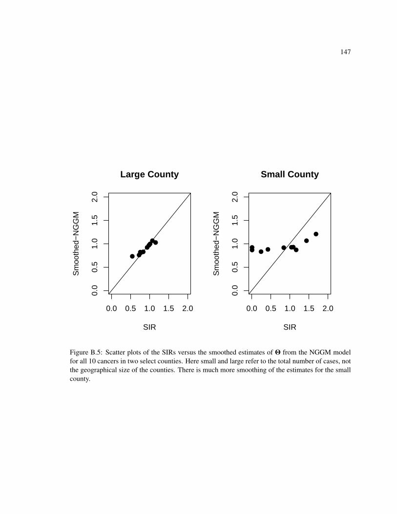
147
●
●
●
● ●●
●
●●●
0.0 0.5 1.0 1.5 2.0
0.0
0.5
1.0
1.5
2.0
Large County
SIR
Sm
ooth
ed−
NG
GM
●
● ●● ●
●●
●● ●
0.0 0.5 1.0 1.5 2.0
0.0
0.5
1.0
1.5
2.0
Small County
SIR
Sm
ooth
ed−
NG
GM
Figure B.5: Scatter plots of the SIRs versus the smoothed estimates of Θ from the NGGM modelfor all 10 cancers in two select counties. Here small and large refer to the total number of cases, notthe geographical size of the counties. There is much more smoothing of the estimates for the smallcounty.

148
Additional Results
Ten-fold cross validation results when ρ is fixed to 0.99 or 0.9 and when π(ρ) is discrete uniform
over {0.05, 0.1, 0.15, . . . , 0.85, 0.9, 0.95, 0.99}.
×105 BIAS2 VAR MSEGGM 1.93 0.79 2.71
NGGM 2.16 0.89 3.05FULL 2.19 0.70 2.89
NFULL 2.61 0.90 3.51
Table B.1: ρ = 0.99
×105 BIAS2 VAR MSEGGM 3.18 0.95 4.13
NGGM 1.89 0.78 2.68FULL 2.17 1.04 3.21
NFULL 3.25 1.07 4.32
Table B.2: ρ = 0.9
×105 BIAS2 VAR MSEGGM 1.59 0.88 2.48
NGGM 3.51 1.67 5.18FULL 3.80 1.71 5.51
NFULL 2.97 1.38 4.35MCAR 1.80 0.99 2.79
Table B.3: π(ρ) is U{0.05, 0.1, 0.15, . . . , 0.85, 0.9, 0.95, 0.99}

149
VITA
Theresa Smith was born to Anne and Walter Smith in McHenry, Illinois. She earned her Bache-
lor of Arts in History and Bachelor of Science in Statistics from the University of Pittsburgh in April,
2009. She enrolled in the Department of Statistics at the University of Washington in September
2009 and earned her Ph.D. in June 2014 under the joint supervision of Adrian Dobra and Jon Wake-
field. She is currently a Senior Research Associate in Spatial Statistics at Lancaster Medical School
in Lancaster, UK.