Copyright (2014) American Institute of Physics. This article may be downloaded for personal use only. Any other use requires prior permission of the author and the American Institute of Physics.

The following article appeared in (J. Chem. Phys., 141, 024506, 2014) and may be found at (http://scitation.aip.org/content/aip/journal/jcp/141/2/10.1063/1.4885365).

The effect of substrate on thermodynamic and kinetic anisotropies in atomic thin filmsAmir Haji-Akbari and Pablo G. Debenedetti

Citation: The Journal of Chemical Physics 141, 024506 (2014); doi: 10.1063/1.4885365 View online: http://dx.doi.org/10.1063/1.4885365 View Table of Contents: http://scitation.aip.org/content/aip/journal/jcp/141/2?ver=pdfcov Published by the AIP Publishing Articles you may be interested in Molecular-dynamics simulations of thin polyisoprene films confined between amorphous silica substrates J. Chem. Phys. 140, 114903 (2014); 10.1063/1.4868231 Properties of model atomic free-standing thin films J. Chem. Phys. 134, 114524 (2011); 10.1063/1.3565480 The two-phase model for calculating thermodynamic properties of liquids from molecular dynamics: Validation forthe phase diagram of Lennard-Jones fluids J. Chem. Phys. 119, 11792 (2003); 10.1063/1.1624057 Effective three-body potentials for Li + (aq) and Mg 2+ (aq) J. Chem. Phys. 119, 7263 (2003); 10.1063/1.1604372 Structure, dynamics, and thermodynamics of benzene-Ar n clusters (1n8 and n=19) J. Chem. Phys. 106, 1530 (1997); 10.1063/1.473301

This article is copyrighted as indicated in the article. Reuse of AIP content is subject to the terms at: http://scitation.aip.org/termsconditions. Downloaded to IP:

128.112.37.74 On: Tue, 19 Aug 2014 20:00:31

THE JOURNAL OF CHEMICAL PHYSICS 141, 024506 (2014)

The effect of substrate on thermodynamic and kinetic anisotropiesin atomic thin films

Amir Haji-Akbari and Pablo G. Debenedettia)

Department of Chemical and Biological Engineering, Princeton University, Princeton, New Jersey 08544, USA

(Received 24 April 2014; accepted 16 June 2014; published online 9 July 2014)

Glasses have a wide range of technological applications. The recent discovery of ultrastable glassesthat are obtained by depositing the vapor of a glass-forming liquid onto the surface of a cold sub-strate has sparked renewed interest in the effects of confinements on physicochemical properties ofliquids and glasses. Here, we use molecular dynamics simulations to study the effect of substrateon thin films of a model glass-forming liquid, the Kob-Andersen binary Lennard-Jones system, andcompute profiles of several thermodynamic and kinetic properties across the film. We observe thatthe substrate can induce large oscillations in profiles of thermodynamic properties such as density,composition, and stress, and we establish a correlation between the oscillations in total density andthe oscillations in normal stress. We also demonstrate that the kinetic properties of an atomic filmcan be readily tuned by changing the strength of interactions between the substrate and the liquid.Most notably, we show that a weakly attractive substrate can induce the emergence of a highly mo-bile region in its vicinity. In this highly mobile region, structural relaxation is several times fasterthan in the bulk, and the exploration of the potential energy landscape is also more efficient. In thesubsurface region near a strongly attractive substrate, however, the dynamics is decelerated and thesampling of the potential energy landscape becomes less efficient than the bulk. We explain thesetwo distinct behaviors by establishing a correlation between the oscillations in kinetic propertiesand the oscillations in lateral stress. Our findings offer interesting opportunities for designing bettersubstrates for the vapor deposition process or developing alternative procedures for situations wherevapor deposition is not feasible. © 2014 AIP Publishing LLC. [http://dx.doi.org/10.1063/1.4885365]

I. INTRODUCTION

A major technological trend of the last few decades hasbeen the shrinkage of accessible time and length scales. Thishas made precision manufacturing of nano-sized particles anddevices easier than ever before. An important consequenceof this trend is the famous “Moore’s Law” which states thatthe computing power of a transistor chip doubles every 18months.1 The physicochemical properties of matter at reducedlength scales can deviate significantly from the bulk. Thesedifferences can be partly attributed to quantum effects thatare only present at such small length scales,2–4 but they canalso be a result of confinement. It is thus practically impor-tant to understand the effect of confinement on the propertiesof atomic and molecular systems. Confined states of matterare not only present in the state-of-the-art technologies, butare also ubiquitous in nature. Confinement plays an impor-tant role in determining the behavior of systems as diverse asbiological cells,5, 6 aquifers,7 natural gas and oil reservoirs,8

and atmospheric droplets and aerosols that constitute clouds.9

Such ubiquity endows the study of confinement in materialswith unusually broad interest.

What is universal about confinement is that it breaks thetranslational isotropy of a bulk material. As a consequence, allphysicochemical properties become functions of position inconfined states of matter. It has indeed been shown in various

a)Electronic mail: pdebene@exchange.princeton.edu

experimental10–15 and computational16–29 studies of confinedmatter that properties such as density, composition, diffusiv-ity, and viscosity can be strong functions of position. Thislack of translational isotropy can lead to major changes in theglobal properties of the corresponding material. For instance,confinement can shift coexistence manifolds in the thermo-dynamic phase diagram of the bulk system, e.g., by loweringthe melting temperature.30–34 It can also induce new phasesthat are not possible in the bulk,35 or can alter the effectivedynamic and mechanical properties of matter such as relax-ation times,14, 32, 36 elastic constants,14, 37, 38 viscosities,20, 38, 39

and diffusivities.28, 40, 41

The translational anisotropy of confined systems can beutilized to produce materials with superior properties. Vapor-deposited ultrastable glasses discovered by Swallen et al.42

are notable examples. Unlike ordinary glasses that are pre-pared via gradual cooling of the bulk supercooled liquid,43, 44

ultrastable glasses are obtained by depositing the vapor of theglass forming substance onto the surface of a substrate witha temperature that is slightly below Tg. The arising glassestend to possess extraordinary thermodynamic and kinetic sta-bility (e.g., higher onset temperature and density). Calorimet-ric experiments reveal that these glasses have lower enthalpiesin comparison to ordinary glasses.42 They thus correspond toconfigurations that have descended deeper along their poten-tial energy landscape than the corresponding “bulk” glasses.Although certain structural features of such low-energy amor-phous configurations, such as the abundance of regular

0021-9606/2014/141(2)/024506/15/$30.00 © 2014 AIP Publishing LLC141, 024506-1

This article is copyrighted as indicated in the article. Reuse of AIP content is subject to the terms at: http://scitation.aip.org/termsconditions. Downloaded to IP:

128.112.37.74 On: Tue, 19 Aug 2014 20:00:31

024506-2 A. Haji-Akbari and P. G. Debenedetti J. Chem. Phys. 141, 024506 (2014)

polyhedral Voronoi cells, have been described in molecularsimulations of model atomic stable glasses,45 considerablegaps in understanding remain regarding the mechanism(s)through which vapor deposition gives rise to such stableconfigurations. It was argued in the original publication ofSwallen et al. that the formation of stable glasses is facili-tated by the existence of a highly mobile region in the growingfree interface, which is a direct consequence of translationalsymmetry breaking in the supercooled liquid. Self-diffusivitymeasurements in organic glasses around the glass transitiontemperature (Tg) have indeed revealed the existence of ahighly mobile region in the vicinity of the free surface, withdiffusivities as large as 106 times the bulk self-diffusivity.13

A similar behavior has been observed in viscosity measure-ments for glassy 3-methylpentane films.12 Also, glassy poly-mer films have been observed to have a highly mobile regionin the vapor-liquid interface at temperatures below Tg.15 Theexistence of such a high mobility region has been observedin molecular simulations of free-standing atomic thin filmsas well.27 It has also been observed that the melting of thesestable glasses proceeds via an interface-initiated growth frontthat develops at interfaces and grows deep into the bulk amor-phous solid.46 The original stable glasses of Swallen et al.were prepared from indomethacin and 1,3-bis-(1-naphthyl)-5-(2-naphthyl)benzene. The same procedure has been usedto prepare stable glasses of other organic molecules such asethylbenzene,47, 48 tuloen,48–51 isopropyl benzene,52 decalin,53

and 1-propanol.54 Also, similar procedures have been used toprepare ultrastable polymeric55 and metallic glasses.56 It hasthus been suggested that the formation of stable glasses viavapor deposition is a universal process that can be used forpreparing stable glasses from any glass-forming substance.57

Glasses have been of considerable technological in-terest even before the discovery of ultrastable glasses,thanks to their high level of structural uniformity, withwidespread applications in areas such as microfluidics,58

energy storage,59, 60 medicine,61–63 photonics and lasertechnology,64–66 lithography,67 spectroscopy,68 tissueengineering,69 and chromatography.70 In most technologicalapplications of glasses, the behavior of the glassy componentis strongly affected by the presence of one or more interfaces.Because of this, and because of the potential role of con-finement in promoting superior stability in vapor-depositedglasses, it is crucial to study translational anisotropy inatomic and molecular thin films. Computer simulations areinvaluable tools in this endeavor since structural and dynam-ical heterogeneities that develop due to lack of translationalisotropy can be probed with much higher resolution insimulations than in experiments.

In this work, we use molecular dynamics simulationin order to perform a systematic investigation of thermody-namic and kinetic anisotropies in thin films of a model atomicglass-forming liquid, the Kob-Andersen binary Lennard-Jones system.71 This paper is organized as follows. We de-scribe the particulars of the system studied in this work inSec. II A. Technical specifications of molecular dynamicssimulations as well as the procedure used for system prepa-ration are presented in Sec. II B. In Sec. II C, we describe thenumerical procedures used for computing position-dependent

thermodynamic and kinetic properties. We present and dis-cuss the computed profiles of those thermodynamic and ki-netic properties in Secs. III A and III B, respectively. Andfinally, Sec. IV is reserved for concluding remarks.

II. METHODS

A. System description and interatomic potential

Figure 1 shows a schematic representation of the simula-tion box that contains a liquid film (depicted in red and green),an attractive substrate (depicted in blue) and a repulsive sub-strate (depicted in yellow). The box is a periodic cuboidal cellstretched along the z direction in order to avoid the film andthe substrates from being affected by their periodic images.The system is made up of four types of atoms (or particles)that have identical masses and interact via the Lennard-Jones(LJ) potential:72

Uαβ(r) = 4εαβ

[(σαβ

r

)12

−(

σαβ

r

)6]

. (1)

All LJ potentials are truncated at a cutoff value of rc,αβ andshifted to zero at rc,αβ . All quantities in this work are ex-pressed in LJ reduced units based on εAA, σ AA, and mA.The interaction parameters for all pairs and the correspond-ing cutoff values are given in Table I. The dimensions ofthe box are given by Lx = Ly = 18 3

√4σAA ≈ 28.57σAA and

Lz = 100 3√

4σAA ≈ 158.74σAA.The liquid film in Fig. 1 is made up of a binary mixture of

A and B atoms that are depicted in red and green, respectively,

FIG. 1. A schematic representation of the simulation box. The liquid film ismade up of red (A) and green (B) atoms, while the blue (C) and yellow (D)atoms comprise the attractive and repulsive substrates, respectively.

This article is copyrighted as indicated in the article. Reuse of AIP content is subject to the terms at: http://scitation.aip.org/termsconditions. Downloaded to IP:

128.112.37.74 On: Tue, 19 Aug 2014 20:00:31

024506-3 A. Haji-Akbari and P. G. Debenedetti J. Chem. Phys. 141, 024506 (2014)

TABLE I. ε, σ and cutoff values for the Lennard-Jones potential.

α β εαβ

σαβ

rc,αβ

A A 1.00 1.00 3.50B B 0.50 0.88 3.08C C εS 1.00 3.50D D εS 1.00 3.50A B 1.50 0.80 2.80A C εS 1.00 3.50A D εS 1.00 1.10B C εS 1.00 3.50B D εS 1.00 1.10C D εS 1.00 3.50

and are mixed at a 4:1 ratio. The A–A, A–B, and B–B in-teraction parameters correspond to the Kob-Andersen binaryLJ mixture.71 The binary mixture arising from this particularchoice of parameters is a liquid that has never been observedto crystallize or phase separate under normal circumstances,73

and is therefore a popular model for studying atomic glass-forming liquids.

The liquid film is in the vicinity of an attractive substratethat is shown in blue in Fig. 1 and is made up of C atomsthat attract A and B atoms with εAC = εBC = εS. Unlike Aand B atoms that are mobile during the course of the molec-ular dynamics simulation, C atoms are located on the sitesof a face-centered cubic (fcc) lattice with a reduced numberdensity of 1.00 and are tethered to their lattice positions usingstiff harmonic springs with spring constant ksσ

2AA/εAA = 103.

In all our simulations, the liquid film is placed close to the[001] face of the fcc crystal. On the opposite side of the at-tractive substrate there is a repulsive substrate made up of Datoms (shown in yellow in Fig. 1). The A–D and B–D LJ in-teractions are truncated and shifted at rc = 1.1σ AD = 1.1σ BDand are therefore purely repulsive. Note that εAD = εBD= εS. D atoms are also placed onto the same fcc lattice oc-cupied by C atoms, and are tethered to their lattice positionswith harmonic springs of equal stiffness. If a single attrac-tive substrate is included, a second liquid film might developon the opposite side of the attractive substrate due to evapo-ration and re-deposition of A and B atoms as a result of theperiodic boundary conditions. By including a second repul-sive substrate, we make sure that the thickest possible film isformed and maintained during the course of the simulation. Inorder to understand the effect of substrate/liquid interactions,we carried out our simulations for three different values of εS,namely, 0.3, 0.5, and 1.0.

B. Molecular dynamics simulations and systempreparation

The molecular dynamics (MD) simulations are per-formed in the NV T ensemble using LAMMPS.74 Newton’sequations of motion are integrated using the velocity Verletalgorithm75 with a time step of �t = 0.0025, and the tem-perature is controlled using the Nosé-Hoover thermostat76, 77

with a time constant of τ = 2.0. For each value of εS,

TABLE II. The dimensions of the fcc lattice and the total number of differ-ent types of atoms in the initial configuration used for system preparation.

Type nx ny nz N

A+B 18 18 10 12 960C 18 18 3.5 4536D 18 18 3 3888

four simulations are performed at the reduced temperaturesT ∗ = 0.6, 0.7, 0.8, and 0.9.

The initial configuration of the system is prepared as fol-lows. The attractive and repulsive substrates are constructedby placing C and D atoms at their corresponding lattice po-sitions. A similar fcc crystal comprised of A atoms is con-structed in the vicinity of the [001] face of the attractive sub-strate, and the identity of each A atom is randomly changed toB with a probability of p = 0.2. The number of atoms used ineach of these lattices is given in Table II. The resulting film isequilibrated in a molecular dynamics simulation in which twoseparate thermostats are used. All substrate atoms are coupledto a thermostat that is set to the final target temperature of thesystem. The mobile A and B atoms, however, are coupled toa second thermostat that is initially set to T ∗ = 0.9, a hightemperature for the Kob-Andersen LJ mixture. During the ini-tial stage of the MD simulation that is performed for 105 MDsteps, the binary LJ crystal melts to become a “hot” liquidfilm. The target temperature of the second thermostat is thengradually decreased to the final target temperature at a rate of10−6/MD step. Eventually, the system is equilibrated for 1.5× 106 MD steps with both thermostats set to the final targettemperature of the system. As will become apparent in Sec. IIIB, the initial melting and the final equilibration times are or-ders of magnitude greater than the largest structural relaxationtimes in all systems simulated in this work. The final configu-rations obtained from the procedure described above are usedfor production runs that are performed in the NV T ensem-ble at the final target temperature. We use an in-house C++computer program that links against the LAMMPS static li-brary to calculate the profiles of thermodynamic and kineticproperties on-the-fly. We sample each trajectory every m MDsteps where m depends on temperature and is larger for lowertemperatures. The numerical procedures used for calculatingthese profiles are presented in Sec. II C.

C. Translational anisotropy and profiles ofthermodynamic and kinetic properties

1. Thermodynamic properties

In order to study the position dependence of thermody-namic properties, the liquid film is partitioned into slices thatare each σ AA/20 thick, and simple time averages of the corre-sponding properties are calculated in each slice. For instance,the density profile of atoms of type α = A, B is given by

ρα(z) = 1

S‖

⟨ Nα∑

i=1

δ(zα,i − z)

⟩, (2)

This article is copyrighted as indicated in the article. Reuse of AIP content is subject to the terms at: http://scitation.aip.org/termsconditions. Downloaded to IP:

128.112.37.74 On: Tue, 19 Aug 2014 20:00:31

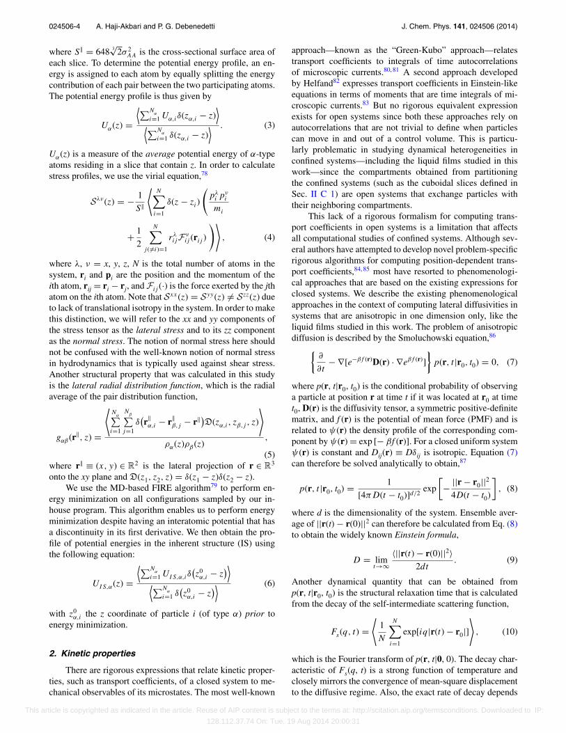
024506-4 A. Haji-Akbari and P. G. Debenedetti J. Chem. Phys. 141, 024506 (2014)

where S‖ = 648 3√

2σ 2AA is the cross-sectional surface area of

each slice. To determine the potential energy profile, an en-ergy is assigned to each atom by equally splitting the energycontribution of each pair between the two participating atoms.The potential energy profile is thus given by

Uα(z) =⟨∑N

α

i=1 Uα,iδ(zα,i − z)⟩

⟨∑Nα

i=1 δ(zα,i − z)⟩ . (3)

Uα(z) is a measure of the average potential energy of α-typeatoms residing in a slice that contain z. In order to calculatestress profiles, we use the virial equation,78

Sλν(z) = − 1

S‖

⟨N∑

i=1

δ(z − zi)

(pλ

i pνi

mi

+ 1

2

N∑j (�=i)=1

rλijF ν

ij (rij )

)⟩, (4)

where λ, ν = x, y, z, N is the total number of atoms in thesystem, ri and pi are the position and the momentum of theith atom, rij = ri − rj, and Fij (·) is the force exerted by the jthatom on the ith atom. Note that Sxx(z) = Syy(z) �= Szz(z) dueto lack of translational isotropy in the system. In order to makethis distinction, we will refer to the xx and yy components ofthe stress tensor as the lateral stress and to its zz componentas the normal stress. The notion of normal stress here shouldnot be confused with the well-known notion of normal stressin hydrodynamics that is typically used against shear stress.Another structural property that was calculated in this studyis the lateral radial distribution function, which is the radialaverage of the pair distribution function,

gαβ(r‖, z) =

⟨N

α∑i=1

Nβ∑

j=1δ(r‖α,i − r‖

β,j − r‖)D(zα,i , zβ,j , z)

⟩

ρα(z)ρβ(z),

(5)where r‖ ≡ (x, y) ∈ R2 is the lateral projection of r ∈ R3

onto the xy plane and D(z1, z2, z) = δ(z1 − z)δ(z2 − z).We use the MD-based FIRE algorithm79 to perform en-

ergy minimization on all configurations sampled by our in-house program. This algorithm enables us to perform energyminimization despite having an interatomic potential that hasa discontinuity in its first derivative. We then obtain the pro-file of potential energies in the inherent structure (IS) usingthe following equation:

UIS,α(z) =⟨∑N

α

i=1 UIS,α,iδ(z0α,i − z

)⟩⟨∑N

α

i=1 δ(z0α,i − z

)⟩ (6)

with z0α,i the z coordinate of particle i (of type α) prior to

energy minimization.

2. Kinetic properties

There are rigorous expressions that relate kinetic proper-ties, such as transport coefficients, of a closed system to me-chanical observables of its microstates. The most well-known

approach—known as the “Green-Kubo” approach—relatestransport coefficients to integrals of time autocorrelationsof microscopic currents.80, 81 A second approach developedby Helfand82 expresses transport coefficients in Einstein-likeequations in terms of moments that are time integrals of mi-croscopic currents.83 But no rigorous equivalent expressionexists for open systems since both these approaches rely onautocorrelations that are not trivial to define when particlescan move in and out of a control volume. This is particu-larly problematic in studying dynamical heterogeneities inconfined systems—including the liquid films studied in thiswork—since the compartments obtained from partitioningthe confined systems (such as the cuboidal slices defined inSec. II C 1) are open systems that exchange particles withtheir neighboring compartments.

This lack of a rigorous formalism for computing trans-port coefficients in open systems is a limitation that affectsall computational studies of confined systems. Although sev-eral authors have attempted to develop novel problem-specificrigorous algorithms for computing position-dependent trans-port coefficients,84, 85 most have resorted to phenomenologi-cal approaches that are based on the existing expressions forclosed systems. We describe the existing phenomenologicalapproaches in the context of computing lateral diffusivities insystems that are anisotropic in one dimension only, like theliquid films studied in this work. The problem of anisotropicdiffusion is described by the Smoluchowski equation,86

{∂

∂t− ∇[e−βf (r)D(r) · ∇eβf (r)]

}p(r, t |r0, t0) = 0, (7)

where p(r, t|r0, t0) is the conditional probability of observinga particle at position r at time t if it was located at r0 at timet0, D(r) is the diffusivity tensor, a symmetric positive-definitematrix, and f (r) is the potential of mean force (PMF) and isrelated to ψ(r) the density profile of the corresponding com-ponent by ψ(r) = exp [− βf (r)]. For a closed uniform systemψ(r) is constant and Dij(r) ≡ Dδij is isotropic. Equation (7)can therefore be solved analytically to obtain,87

p(r, t |r0, t0) = 1

[4πD(t − t0)]d/2exp

[− ||r − r0||2

4D(t − t0)

], (8)

where d is the dimensionality of the system. Ensemble aver-age of ||r(t) − r(0)||2 can therefore be calculated from Eq. (8)to obtain the widely known Einstein formula,

D = limt→∞

〈||r(t) − r(0)||2〉2dt

. (9)

Another dynamical quantity that can be obtained fromp(r, t|r0, t0) is the structural relaxation time that is calculatedfrom the decay of the self-intermediate scattering function,

Fs(q, t) =⟨

1

N

N∑i=1

exp[iq|r(t) − r0|]⟩

, (10)

which is the Fourier transform of p(r, t|0, 0). The decay char-acteristic of Fs(q, t) is a strong function of temperature andclosely mirrors the convergence of mean-square displacementto the diffusive regime. Also, the exact rate of decay depends

This article is copyrighted as indicated in the article. Reuse of AIP content is subject to the terms at: http://scitation.aip.org/termsconditions. Downloaded to IP:

128.112.37.74 On: Tue, 19 Aug 2014 20:00:31

024506-5 A. Haji-Akbari and P. G. Debenedetti J. Chem. Phys. 141, 024506 (2014)

on q and is typically largest for q = qmax , the wavevector cor-responding to the first peak of the structure factor S(q). Struc-tural relaxation times are typically obtained by finding theroot of Fs(qmax , τ ) = c with c, being a constant that shouldbe chosen so that it falls into the alpha relaxation region. Forthree-dimensional systems c is generally chosen to be 1/e.

In confined systems that are anisotropic along the z di-rection however, D(z) is no longer isotropic and has two dis-tinct elements instead: D‖(z) = Dxx(z) = Dyy(z) or the lateraldiffusivity and D⊥(z) = Dzz(z) or the normal diffusivity. Thez dependence of both these diffusivities turns Eq. (8) into acoupled partial differential equation that cannot be solved viaconventional techniques such as separation of variables eventhough ψ(z) can be accurately determined from a molecularsimulation. Several closed-form analytical solutions of Eq. (8)have been reported by making certain a priori assumptionsabout the mathematical form of D(z).88 But since D‖(z) andD⊥(z) are not a priori known, it is only possible to obtain anumerical solution that relates position-dependent diffusivi-ties and the observed p(r‖, z, t|0, z0, t0) in a self-consistentmanner. In order to avoid this tedious path, different authorshave taken different phenomenological approaches for calcu-lating D‖ profiles. In all of these approaches, the simulationdomain is divided into slices, and an ad hoc mean-squareddisplacement, φ(z, t), is defined for every slice, which, along-side Eq. (9), is used to determine lateral diffusivities in eachslice.

A common phenomenological approach used by manyauthors25, 27 is to apply the virtual absorbing boundary con-ditions at the boundaries of each slice. In this approach, theentities that leave and re-enter a slice during a time windowdo not contribute to the mean-square displacement of thattime window since they might spend time in slices with diffu-sivities different from that of the slice of interest. Therefore,φ(z, t) is defined as

φ(z, t) = 〈|r‖(t) − r‖(0)|2〉|z(τ )−z|< �z2 ,0≤τ≤t , (11)

with �z being the thickness of the slice. This approach isnumerically costly since the fraction of particles that do notleave their initial slice during a time interval t will decreasewith t. As a result, it is far more difficult to gather qual-ity statistics in the long-term diffusive regime of the mean-squared displacement. Another problem with this approachis the sensitivity of the computed relaxation times and diffu-sivities to the slice thickness due to unacceptable biasing infavor of less mobile particles that are more likely to remaininside a thinner slice. Considering these limitations, someauthors have used alternative phenomenological approaches.One possibility is to define φ(z, t) based on the position of theparticle at the beginning of the time window,23, 26

φ(z, t) = 〈|r‖(t) − r‖(0)|2δ[z(0) − z] 〉. (12)

A second possibility is to include in φ(z, t) only the par-ticles that are present in the slice both in the beginning and atthe end of the time window,24

φ(z, t) = 〈|r‖(t) − r‖(0)|2D(z(0), z(t), z) 〉. (13)

And finally, a third possibility is to assign the contribution ofevery particle to the φ(z, t) that corresponds to its average

normal position z̄(t) = (1/t)∫ t

0 z(τ )dτ throughout the timewindow t,19

φ(z, t) = 〈|r‖(t) − r‖(0)|2δ[z̄(t) − z]〉. (14)

Although arguments can be raised for and against any of theseapproaches, there is no solid theoretical reason for preferringany one of them over others. In this work, we adopt the ap-proach expressed in Eq. (13) due to its computational simplic-ity and its robustness to changes in the slice thickness. Also,by only allowing the particles that are present in the sameslice both at the beginning and at the end of a time window tocontribute to φ(z, t), we avoid the unphysical biasing towardsparticles that persistently move away from their initial slicestowards regions of different diffusivities.

Another difficulty in calculating position-dependent dif-fusivities is the inter-slice mixing that occurs at very largetime windows. This leads to an apparent super-diffusiveregime in the ad hoc φ(z, t) at large values of t since atlarger time windows, the particles are more likely to take around-trip to slices that are far away from their slice of origin(Fig. 2). As a consequence, D‖(z)’s cannot be computed fromthe asymptotic behavior of φ(z, t) and should instead be es-timated from the diffusive regime that precedes the mixing-initiated super-diffusive regime. In Fig. 2, for instance, thiswill correspond to 100 ≤ t ≤ 102.

Using the same convention introduced above, a similarslice scattering function can be defined as follows:

Fs(q, z, t)= 1

N

⟨N∑

i=1

exp{iq|�r‖(t)|}D(z(t), z(0), z)

⟩. (15)

As previously observed in molecular simulations of two-dimensional systems,89 self-intermediate scattering functionscan take lower values during the caging regime in two-dimensional systems than in three-dimensional systems.Therefore, the cutoff value for defining relaxation timesneeds to be smaller in two-dimensional systems, including forFs(q, z, t)’s calculated in this work. We will therefore use avalue of c = 0.2, which always falls in the alpha relation re-gion for all scattering functions calculated in this work.

Another ambiguity that arises in computing structural re-laxation times in confined systems is the sensitivity of thecalculated relaxation time profiles to the particular value of

%

z/σAA = 1.0

z/σAA = 3.0z/σAA = 6.0

10−2 10−1 100 101 102 103 104

10−2

100

102

104

106

10−4

t

φ(z,

t)

FIG. 2. Total mean-squared displacements computed for a film withεS = 0.3 at T ∗ = 0.9. The super diffusive regime at t ≈ 103 is due to theinter-slice mixing of particles.

This article is copyrighted as indicated in the article. Reuse of AIP content is subject to the terms at: http://scitation.aip.org/termsconditions. Downloaded to IP:

128.112.37.74 On: Tue, 19 Aug 2014 20:00:31

024506-6 A. Haji-Akbari and P. G. Debenedetti J. Chem. Phys. 141, 024506 (2014)

Distance from the Substrate (σAA)4 8 12 160

100

101

Rel

axat

ion

Tim

e τΑ , q*σAA = 7.251

τtotal , q*σAA = 7.251τB , q*σAA = 7.251

τΑ , q*σAA = 5.0

τtotal , q*σAA = 5.0τB , q*σAA = 5.0

FIG. 3. The sensitivity of τ ‖(z) to the particular choice of q. The lateral re-laxation times are computed at two values of q for a film with εS = 0.3 andT ∗ = 0.9. Although the precise value of τ ‖(z) depends on q, the observedtrend is independent of the particular choice of q.

q as the rate of decay in Fs(q, z, t) depends on q. Since sig-nificant structural variations are possible in a confined sys-tem, e.g., due to density and composition oscillations, theposition of the first peak of S(q, z) can be a strong functionof z. However, using different wavenumbers for different re-gions of space can make comparing the computed relaxationtimes nontrivial. As a matter of consistency, we use a sin-gle q∗ value (q∗ = 7.251σ−1

AA) for all our calculations, and weconfirm the robustness of computed relaxation time profilesby computing lateral diffusivities that are independent of thechoice of q∗. We also confirm that relaxation time profilesare qualitatively insensitive to the particular choice of q∗ andthe observed trends are preserved if different values of q∗ areused even though the exact numerical values of τ ‖ will change(Fig. 3).

Due to the constraint imposed in Eqs. (13) and (15), onlya fraction of trajectories contribute to φ(z, t) and Fs(q, z, t)calculations. As a result, it is more difficult to obtain qual-ity statistics in computing these autocorrelation functions. Wetherefore use thicker slices (�z = σ AA/4) for computing pro-files of dynamical quantities.

III. RESULTS AND DISCUSSION

A. Thermodynamic properties

Figure 4 depicts density profiles computed for severalvalues of T ∗ and εS. We observe that the liquid is alwaysstratified in the vicinity of the substrate, although the extentof stratification, i.e., the number and the amplitude of densitywaves, increases by increasing εS or by decreasing the tem-perature. The oscillations in density are both observed for thetotal density profile (shown in black) as well as the densityprofiles of individual components (shown in red and green).The emergence of layering in the vicinity of a substrate hasbeen previously observed in a wide variety of other confinedsystems such as slit pores17 and molecular thin films29 andcan be attributed to non-random ordering of mobile atomsof the liquid in the close vicinity of immobile atoms of thesubstrate. These density waves can therefore be conceptuallythought of as (unnormalized) substrate-liquid radial distribu-tion functions that are frozen due to the freezing of the atomsin the substrate.

The oscillatory density profile of the liquid near the sub-strate might or might not be accompanied by crystalline order.These two can be distinguished by inspecting the lateral radialdistributions computed from Eq. (5). In a slice that is later-ally amorphous, gαβ (r, z) converges to unity as r → ∞ withdecaying fluctuations, while in a slice with lateral crystallineorder, the fluctuations of gαβ(r, z) persist over arbitrarily longdistances. In order to quantify these two distinct behaviors,we compute the following function for every slice:

fαβ(rc, z; ν) =∫ r

c

0H

(∣∣gαβ(r, z) − 1∣∣ − ν

)dr, (16)

with H (x) = ∫ x

−∞ δ(ξ )dξ , the Heaviside function. For amor-phous slices, fαβ(rc, z; ν) will be independent of rc for suf-ficiently large values of rc since the amplitude of deviationsfrom unity will be smaller than ν > 0 when r is large enough.For crystalline slices, however, fαβ(rc, z; ν) will grow withrc indefinitely since the characteristic amplitude of deviationsfrom unity will be always larger than a sufficiently smallν > 0. We thus define the crystalline region as the part of

Total A B Total A B Total A B Total A B

Total A B

Total A B

Total A B

Total A B

Total A B

Total A B

Total A B

Total A B

0 4 8 12 16 4 8 12 16 4 8 12 16 4 8 12 16Distance from the Substrate (σAA)

0.00.40.81.20.0

1.0

2.00.0

2.0

4.0

6.0

Num

ber D

ensi

ty

T*= 0.6 T*= 0.7 T*= 0.8 T*= 0.9

εS = 1.0

εS = 0.5

εS = 0.3

FIG. 4. Density profiles of thin films as a function of distance from the substrate. The crystalline regions of the films are shaded in light blue.

This article is copyrighted as indicated in the article. Reuse of AIP content is subject to the terms at: http://scitation.aip.org/termsconditions. Downloaded to IP:

128.112.37.74 On: Tue, 19 Aug 2014 20:00:31

024506-7 A. Haji-Akbari and P. G. Debenedetti J. Chem. Phys. 141, 024506 (2014)

0 1 2 3 4 5Distance from the Substrate (σAA)

2π σ2 A

A

rc

0

|g(r

/σA

A)−

1|rd

rrc/σAA = 14.0rc/σAA = 13.0rc/σAA = 12.0rc/σAA = 11.0rc/σAA = 10.0rc/σAA = 9.0rc/σAA = 8.0rc/σAA = 7.0rc/σAA = 6.0rc/σAA = 5.0rc/σAA = 4.0

0

0.5

1.0

1.5

2.0

FIG. 5. Determining the thickness of the crystalline region in the vicinityof the substrate for T ∗ = 0.6 and εS = 1.0. The arrow corresponds to thesmallest z for which f (rc, z; 0.05) becomes independent of rc.

the film where f (rc, z; ν) changes with rc. This procedure isdepicted in Fig. 5, where f (rc, z; 0.05) vs. z is given for afew different values of rc in the simulation conducted at T ∗

= 0.6 and εS = 1.0. Since there is no noticeable dependenceof f (rc, z; ν) on rc for z ≥ ζ = 3.2σ AA, we define the regionz/σ AA ∈ [0, 3.2] as the crystalline region of the film. We usethe same procedure for determining the widths of crystallineregions (ζ ) at other values of T ∗ and εS, and show those re-gions in shaded light blue in Figs. 4 and 9–12. Similar valuesare obtained for ζ if gAA(r, z) or gBB(r, z) are used insteadof gtotal(r, z). As can be vividly seen in Fig. 4, the width ofthe crystalline region is always significantly smaller than thewidth of the stratified region, which shows that crystallinityis not a necessary condition for layering in the vicinity of asubstrate. Also the width of the crystalline region increasesby decreasing the temperature or by increasing εS.

In order to understand the origin of these density oscilla-tions, we inspect the normal stress profiles computed fromEq. (4) and depicted in Fig. 6. The normal stress profilesare oscillatory for all the temperatures and εS’s studied inthis work, with the depth and amplitude of oscillations in-creasing upon an increase in εS or 1/T. (As discussed inSec. III B and depicted in Fig. 14, a similar behavior is ob-served for oscillations in lateral stress.) Stress oscillations can

&

&

&

&

0 4 8 12 16−2.0

Nor

mal

Str

ess

Distance from the Substrate (σAA)

T* = 0.6T* = 0.7T* = 0.8T* = 0.9

T* = 0.6T* = 0.7T* = 0.8T* = 0.9

T* = 0.6T* = 0.7T* = 0.8T* = 0.9

−1.0

0.0

1.0

−2.0

−1.0

0.0

1.0

2.0

−20

−10

0

10

20ε

S = 1.0 ε

S = 0.5 ε

S = 0.3

FIG. 6. Normal stress profiles for selected values of εS and temperature.

be relatively strong in the crystalline regions of the films, abehavior expected considering the anisotropic nature of crys-tals. In amorphous regions of the films however, a direct cor-relation is observed between density and normal stress, withpeaks and valleys of ρ(z) closely following the peaks and val-leys of Szz(z) (Fig. 7). This is consistent with the behavior of amechanically stable fluid that becomes denser upon compres-sion. At higher values of normal stress, that can be thought as

&

&

−2.0

Num

ber D

ensi

tyN

orm

al S

tres

s (a)

0Distance from the Substrate (σAA)

4 8 12 16

0.4

0

0.8

1.2

−1.0

0.0

1.0+ + + + + +

−10

0

10

20

0Distance from the Substrate (σAA)

4 8 12 160

2

4

6

Num

ber D

ensi

tyN

orm

al S

tres

s

+ + + + (b)

Total A B Total A B

FIG. 7. Density and normal stress profiles for (a) εS = 0.3, T ∗ = 0.6 and (b) εS = 1.0, T ∗ = 0.6. Regions with lateral long-range order are shaded in blue. Inamorphous parts of the film, regions with positive and negative normal stress are shaded in green and red, respectively.

This article is copyrighted as indicated in the article. Reuse of AIP content is subject to the terms at: http://scitation.aip.org/termsconditions. Downloaded to IP:

128.112.37.74 On: Tue, 19 Aug 2014 20:00:31

024506-8 A. Haji-Akbari and P. G. Debenedetti J. Chem. Phys. 141, 024506 (2014)

0 4 8 12 16Distance from the Substrate (σAA)

T* = 0.6T* = 0.7T* = 0.8T* = 0.9

T* = 0.6T* = 0.7T* = 0.8T* = 0.9

T* = 0.6T* = 0.7T* = 0.8T* = 0.9

B M

ole

Frac

tion

εS = 1.0

εS = 0.5

εS = 0.3

0

0.1

0.2

0.30

0.2

0.4

0.60

0.4

0.8

FIG. 8. The mole fraction of B vs. distance from the substrate for severalvalues of temperature and εS.

the pressure in the z direction, we expect an increase in ρ(z),the marginal—or plane-averaged—density in the z direction.Note that this correlation does not hold in the crystalline re-gion (e.g., Fig. 7(b)), since crystals react to stress in nontrivialways.

Figure 8 depicts the mole fraction of B, xB = ρB/(ρA+ ρB), as a function of distance from the substrate. We ob-serve that the B particles tend to avoid both the liquid-vaporand the liquid solid interfaces. In systems with attractive in-teractions, the formation—and the maintenance—of a free in-

terface would involve an energetic cost arising from the lossof half the nearest neighbor interactions for the particles atthe interface. As can be clearly seen in potential energy pro-files depicted in Fig. 9, the average energy of both particletypes increases in the vicinity of the vapor-liquid interface,which is an indication of this energetic loss. But this energeticloss is not sufficient for explaining composition differencesin multicomponent systems as different composition profilescan give rise to different overall mixing entropies. As shownin detail in Appendix A, an A-rich interfacial region—andthus a B-rich bulk region—will lead to an overall increase inthe mixing entropy, which can offset the energetic loss at theinterface.

Due to the presence of attractive A–C and B–C interac-tions, the energetic cost of maintaining a liquid/substrate in-terface is smaller, and can be close to non-existent for stronglyattractive “sticky” substrates (e.g., εS = 1.0). Indeed, the aver-age potential energies of both A and B atoms increase in thevicinity of “loose” substrates (i.e., substrates with εS = 0.3and 0.5), but not to the level of the atoms in the free interface.As a result, we observe an A-rich region in the immediatevicinity of the substrate in all our simulations. However, themole fraction of B atoms in the interfacial region increases byincreasing εS. This is because the energetic loss is smaller forsubstrates that are more sticky.

Like the profiles of total density, composition profiles areoscillatory near the substrate and xB undergoes large fluctu-ations before converging to its bulk value. Also the ampli-tudes and the number of composition waves are larger at lowertemperatures and larger εS’s. For sticky substrates (εS = 1.0)and low temperatures (T ∗ ≤ 0.7), the crystalline region inthe vicinity of the substrate is phase-separated into crystallinesheets of A atoms followed by crystalline sheets of B atoms(Top panel of Fig. 8).

Figure 9 depicts the potential energy profiles calculatedfrom Eq. (6) for different values of T ∗ and εS. Unlike den-sities, compositions, and lateral and normal stresses that al-ways undergo significant oscillations near the substrate, po-tential energies tend to increase monotonically in the vicinityof loose substrates, i.e., for εS = 0.3, and only oscillate near

&

%

%

&

%

&

%

%

&

%%

%% %% %%

&&&

%%

&&&

0 4 8 12 0 4 8 12 0 4 8 12 0 4 8 12 16Distance from the Substrate (σAA)

−9

−6

−3

0

−6

−3

0

−6

−3

0

Pote

ntia

l Ene

rgy

Total A B Total A B Total A B Total A B

Total A B Total A B Total A B Total A B

Total A B Total A B Total A B Total A B

T*= 0.6 T*= 0.7 T*= 0.8 T*= 0.9

εS = 1.0

εS = 0.5

εS = 0.3

FIG. 9. Potential energy profiles of thin films as a function of distance from the substrate. The crystalline regions of the films are shaded in light blue.

This article is copyrighted as indicated in the article. Reuse of AIP content is subject to the terms at: http://scitation.aip.org/termsconditions. Downloaded to IP:

128.112.37.74 On: Tue, 19 Aug 2014 20:00:31

024506-9 A. Haji-Akbari and P. G. Debenedetti J. Chem. Phys. 141, 024506 (2014)

0 4 8 12 0 4 8 12 0 4 8 12Distance from the Substrate (σAA)

Total A B Total A B Total A B Total A B

Total A B Total A B Total A B Total A B

Total A B Total A B Total A B Total A B

T*= 0.6 T*= 0.7 T*= 0.8 T*= 0.9

εS = 1.0

εS = 0.5

εS = 0.3

0 4 8 12 160123012301234

Uα(z

)−

UIS

,α(z

)

FIG. 10. Profile of 〈U〉 − 〈U〉IS of thin films as a function of distance from the substrate. The crystalline regions of the films are shaded in light blue.

sticky substrates (εS = 1.0). For moderately attracting sub-strates (εS = 0.5), two distinct regimes are observed at dif-ferent temperatures. At higher temperatures (T ∗ ≥ 0.8), po-tential energy profiles are monotonic and are like the onesobserved for εS = 0.3. For lower temperatures, however, theyare more oscillatory near the substrate, like the ones observedfor sticky substrates. The emergence of oscillatory potentialenergy profiles can be attributed to the strong ordering in-duced by these sticky substrates, something that also mani-fests itself in stronger oscillations in density, stress, and com-position profiles. This effect is much weaker in the vicinityof looser substrates, giving rise to more monotonic potentialenergy profiles.

Figure 10 depicts Uα(z) − UIS, α(z) for different values ofT ∗ and εS. This quantity—that we call the dive profile—is theaverage energy that particles of type α residing at z, lose asa result of energy minimization, and is a measure of the ef-ficiency with which particles of a certain region can explorethe potential energy landscape. We observe larger values of

Uα(z) − UIS, α(z) in the vicinity of the vapor-liquid interface,which corresponds to more efficient sampling of the potentialenergy landscape by these particles. This has also been ob-served in computational studies of free-standing thin films ofthe Kob-Andersen LJ mixture.27 A similar maximum is ob-served in the subsurface region neighboring loose substrates.In the vicinity of sticky substrates, however, the potential en-ergy landscape is more heavily affected by the presence ofthe substrate, and the particles are more restricted in samplingand exploring that oscillatory landscape. Similar to potentialenergy profiles, dive profiles are also very oscillatory in thevicinity of sticky substrates, which is also a consequence ofstrong substrate-induced ordering in those regions. Anotherinteresting observation is the gradual mild decline of Uα(z)− UIS, α(z) across the films that are in the vicinity of stickysubstrates. This shows that the ordering effect of a stronglyattractive substrate extends far beyond the solid/liquid sub-surface region. This “deep” ordering induced by sticky wallsalso manifests itself in stronger stratification in the liquid film.

Rel

axat

ion

Tim

e

0 4 8 12 0 4 8 12 0 4 8 12 0 4 8 12 16Distance from the Substrate (σAA)

100

T*= 0.6 T*= 0.7 T*= 0.8 T*= 0.9

εS = 1.0

εS = 0.5

εS = 0.3

101

100

101

100

101

102Total A B Total A B Total A B Total A B

Total A B Total A B Total A B Total A B

Total A B Total A B Total A B Total A B

FIG. 11. Relaxation time profiles of thin films as a function of distance from the substrate as calculated from the self-intermediate scattering functions. Thecrystalline regions of the films are shaded in light blue.

This article is copyrighted as indicated in the article. Reuse of AIP content is subject to the terms at: http://scitation.aip.org/termsconditions. Downloaded to IP:

128.112.37.74 On: Tue, 19 Aug 2014 20:00:31

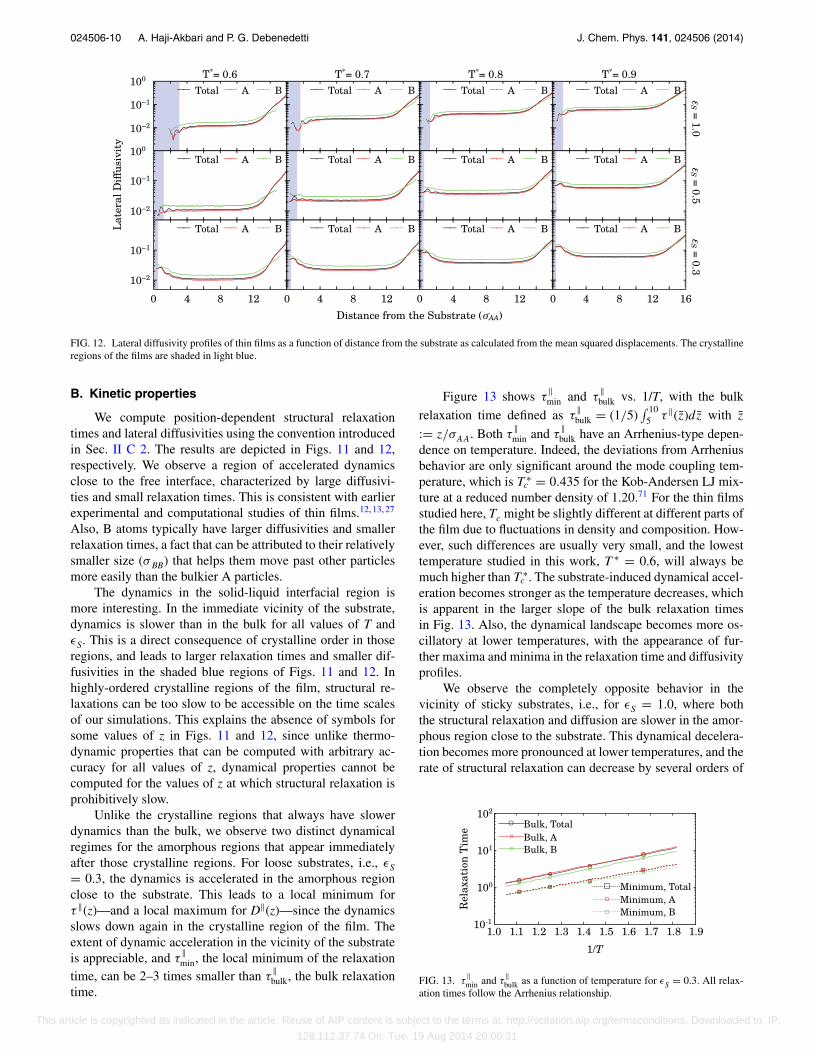
024506-10 A. Haji-Akbari and P. G. Debenedetti J. Chem. Phys. 141, 024506 (2014)

00 4 8 12 0 4 8 12 0 4 8 12 4 8 12 16Distance from the Substrate (σAA)

10−2

Late

ral D

ius

ivity

εS = 1.0

εS = 0.5

εS = 0.3

T*= 0.6 T*= 0.7 T*= 0.8 T*= 0.9

10−1

10−2

10−1

100

10−2

10−1

100Total A B Total A B Total A B Total A B

Total A B Total A B Total A B Total A B

Total A B Total A B Total A B Total A B

FIG. 12. Lateral diffusivity profiles of thin films as a function of distance from the substrate as calculated from the mean squared displacements. The crystallineregions of the films are shaded in light blue.

B. Kinetic properties

We compute position-dependent structural relaxationtimes and lateral diffusivities using the convention introducedin Sec. II C 2. The results are depicted in Figs. 11 and 12,respectively. We observe a region of accelerated dynamicsclose to the free interface, characterized by large diffusivi-ties and small relaxation times. This is consistent with earlierexperimental and computational studies of thin films.12, 13, 27

Also, B atoms typically have larger diffusivities and smallerrelaxation times, a fact that can be attributed to their relativelysmaller size (σ BB) that helps them move past other particlesmore easily than the bulkier A particles.

The dynamics in the solid-liquid interfacial region ismore interesting. In the immediate vicinity of the substrate,dynamics is slower than in the bulk for all values of T andεS. This is a direct consequence of crystalline order in thoseregions, and leads to larger relaxation times and smaller dif-fusivities in the shaded blue regions of Figs. 11 and 12. Inhighly-ordered crystalline regions of the film, structural re-laxations can be too slow to be accessible on the time scalesof our simulations. This explains the absence of symbols forsome values of z in Figs. 11 and 12, since unlike thermo-dynamic properties that can be computed with arbitrary ac-curacy for all values of z, dynamical properties cannot becomputed for the values of z at which structural relaxation isprohibitively slow.

Unlike the crystalline regions that always have slowerdynamics than the bulk, we observe two distinct dynamicalregimes for the amorphous regions that appear immediatelyafter those crystalline regions. For loose substrates, i.e., εS= 0.3, the dynamics is accelerated in the amorphous regionclose to the substrate. This leads to a local minimum forτ ‖(z)—and a local maximum for D‖(z)—since the dynamicsslows down again in the crystalline region of the film. Theextent of dynamic acceleration in the vicinity of the substrateis appreciable, and τ

‖min, the local minimum of the relaxation

time, can be 2–3 times smaller than τ‖bulk, the bulk relaxation

time.

Figure 13 shows τ‖min and τ

‖bulk vs. 1/T, with the bulk

relaxation time defined as τ‖bulk = (1/5)

∫ 105 τ ‖(z̄)dz̄ with z̄

:= z/σAA. Both τ‖min and τ

‖bulk have an Arrhenius-type depen-

dence on temperature. Indeed, the deviations from Arrheniusbehavior are only significant around the mode coupling tem-perature, which is T ∗

c = 0.435 for the Kob-Andersen LJ mix-ture at a reduced number density of 1.20.71 For the thin filmsstudied here, Tc might be slightly different at different parts ofthe film due to fluctuations in density and composition. How-ever, such differences are usually very small, and the lowesttemperature studied in this work, T ∗ = 0.6, will always bemuch higher than T ∗

c . The substrate-induced dynamical accel-eration becomes stronger as the temperature decreases, whichis apparent in the larger slope of the bulk relaxation timesin Fig. 13. Also, the dynamical landscape becomes more os-cillatory at lower temperatures, with the appearance of fur-ther maxima and minima in the relaxation time and diffusivityprofiles.

We observe the completely opposite behavior in thevicinity of sticky substrates, i.e., for εS = 1.0, where boththe structural relaxation and diffusion are slower in the amor-phous region close to the substrate. This dynamical decelera-tion becomes more pronounced at lower temperatures, and therate of structural relaxation can decrease by several orders of

1.010-1

100

101

102

1/T

Rel

axat

ion

Tim

e Bulk, TotalBulk, ABulk, B

Minimum, TotalMinimum, AMinimum, B

1.1 1.2 1.3 1.4 1.5 1.6 1.7 1.8 1.9

FIG. 13. τ‖min and τ

‖bulk as a function of temperature for εS = 0.3. All relax-

ation times follow the Arrhenius relationship.

This article is copyrighted as indicated in the article. Reuse of AIP content is subject to the terms at: http://scitation.aip.org/termsconditions. Downloaded to IP:

128.112.37.74 On: Tue, 19 Aug 2014 20:00:31

024506-11 A. Haji-Akbari and P. G. Debenedetti J. Chem. Phys. 141, 024506 (2014)

&

&

&

T* = 0.6T* = 0.7T* = 0.8T* = 0.9

T* = 0.6T* = 0.7T* = 0.8T* = 0.9

T* = 0.6T* = 0.7T* = 0.8T* = 0.9

Late

ral S

tres

s

0Distance from the Substrate (σAA)

−10.0

0.0

5.0

−2.0

−1.0

0.0

1.0

−1.0

0.0

−2.04 8 12 16

−5.0

−1.5

−0.5

0.5

εS = 1.0

εS = 0.5

εS = 0.3

FIG. 14. Lateral stress profiles for several values of εS and temperature.

magnitude, as can be seen in the top panels of Figs. 11 and 12.Also the dynamical landscape of the film is highly oscillatory,with diffusivity and relaxation time profiles showing severalmaxima and minima across the film.

For εS = 0.5, namely, a moderately attractive substrate,the qualitative features of the observed dynamical regime de-pend on temperature. At higher temperatures, the dynamicsis accelerated in the amorphous region close to the substrate,similar to the behavior observed for εS = 0.3. However, themagnitude of this dynamical acceleration is smaller. At T ∗

= 0.9, for instance, τ‖bulk/τ

‖min ≈ 1.52 which is smaller than

2.01, the value observed for εS = 0.3 at the same temperature.Upon decreasing temperature, this dynamical acceleration be-comes weaker and weaker, until a cross-over occurs at T ∗

≈ 0.7 where a shift to the substrate-induced decelerated dy-namics is observed.

These two distinct dynamical regimes can be explainedby inspecting the lateral stress profiles depicted in Fig. 14.Like the normal stress that is a pressure in the z direction,lateral stress is a pressure in the xy plane. In simple fluids, dy-namics become slower at higher pressures. It is therefore nat-ural to expect that higher lateral stress will also lead to slowerlateral dynamics. As can be seen in Fig. 15, oscillations ofdynamical properties closely follow the oscillations in lateralstress. The dynamical acceleration in the vicinity of weaklyattractive substrates can therefore be attributed to tensile lat-eral stress in those regions, while in the vicinity of stronglyattractive substrates, the lateral stress is typically compres-sive, which leads to a slowdown in dynamics. The tempera-ture dependence of these two dynamical regimes can also beexplained by inspecting the lateral stress profiles. As temper-ature decreases, the magnitude of tensile or compressive lat-eral stress becomes larger. As a consequence, the accelerationor deceleration of dynamics (with respect the bulk) becomesstronger as well.

Unlike the oscillations in thermodynamic properties thatcan extend deep into the bulk region of the film, dynamicalproperties tend to converge much more quickly to their bulk

&&&

Distance from the Substrate (σAA)4 8 12 160

100

101

0.0

−1.0

−2.0

10−2

10−1

Late

ral S

tres

sR

elax

atio

n Ti

me

Di

usiv

ity

Distance from the Substrate (σAA)4 8 12 160

10−3

10−2

10−1

−2.0

0.0

2.0

100

101

102

Late

ral S

tres

sR

elax

atio

n Ti

me

Di

usiv

ity

(a) (b)Total A B

Total A B

Total A B

Total A B

FIG. 15. Lateral stress vs. dynamical properties for (a) T ∗ = 0.6, εS = 0.3 and (b) T ∗ = 0.9, εS = 1.0. The crystalline regions of the films are shaded in blue,while the amorphous regions with positive and negative lateral stress are shaded in green and red, respectively.

This article is copyrighted as indicated in the article. Reuse of AIP content is subject to the terms at: http://scitation.aip.org/termsconditions. Downloaded to IP:

128.112.37.74 On: Tue, 19 Aug 2014 20:00:31

024506-12 A. Haji-Akbari and P. G. Debenedetti J. Chem. Phys. 141, 024506 (2014)

1.2 1.4 1.61.3 1.51/T

100

101

Rel

axat

ion

Tim

e

(a) (b) (c)

1.2 1.4 1.61.3 1.51/T

1.2 1.4 1.61.3 1.51/T

εS = 0.3 εS = 0.5 εS = 1.0

εS = 0.3 εS = 0.5 εS = 1.0

εS = 0.3 εS = 0.5 εS = 1.0

FIG. 16. Temperature dependence of bulk relaxation times. Panels (a) and (b) correspond to the A (◦) and B (�) particles, respectively, while panel (c) givesthe total (�) bulk relaxation times.

values. As a result, bulk relaxation times can be readily cal-culated for all the films studied in this work. For εS = 0.3and εS = 0.5, relaxation times converge to the bulk valuerelatively quickly. We therefore define the bulk relaxationtime as the average relaxation time for 5 ≤ z/σ AA ≤ 10. ForεS = 1.0 however, this convergence is slower and occurs at afurther distance from the substrate. We therefore use the range6 ≤ z/σ AA ≤ 10 for this calculation. Figure 16 depicts the tem-perature dependence of τ

‖bulk. The temperature dependence is

satisfactorily described by the Arrhenius relationship, whichis not surprising considering the relatively high temperaturesstudied in this work.

IV. CONCLUSIONS

In this work, we find that a substrate can induce large os-cillations in a wide range of thermodynamic and kinetic prop-erties across a film. Properties such as density, composition,and stress can undergo large oscillations near a substrate. Weexplain the emergence of density waves by establishing a cor-relation between density oscillations and normal stress oscil-lations. This is in line with our intuition that mechanically sta-ble fluids become denser in the presence of compressive nor-mal stress. We also propose a simple thermodynamic model toexplain the preference of B atoms to avoid interfacial regions.Unlike densities, compositions, and stresses, we observe po-tential energy profiles to oscillate only in the vicinity of stickysubstrates.

We investigate dynamical anisotropies of the film bycomputing position-dependent diffusivities and relaxationtimes and discover two distinct dynamical regimes in thevicinity of the substrate. For sticky substrates and/or lowtemperatures, structural relaxation is decelerated in the solid-liquid interfacial region, a behavior that is in accordance withour intuition that a substrate will lead to dynamical decelera-tion. For loose substrates and/or high temperatures, however,we observe a counter-intuitive acceleration of dynamics in theamorphous liquid near the substrate. We explain both theseregimes by studying lateral stress profiles across the film andestablish a strong correlation between the oscillations in lat-eral stress and the oscillations in the corresponding kineticproperties.

Consequently, two distinct qualitative behaviors are ob-served for energetics and dynamics in the vicinity of attrac-tive substrates that are summarized in Fig. 17. Looser sub-strates are characterized by faster dynamics, a monotonic in-crease in potential energy, and a more efficient exploration of

the potential energy landscape in subsurfaces of solid-liquidinterfaces. In this context, the behavior of the solid-liquid sub-surface is very similar to that of the vapor-liquid subsurfaceobserved in earlier computational studies of free-standing thinfilms.27 Near sticky substrates however, we observe the com-pletely opposite regime, characterized by strong ordering,slower dynamics, and an oscillatory potential energy land-scape in the solid-liquid subsurface region. For moderately in-teracting substrates, both these regimes are possible depend-ing on temperature. These findings are very important in thecontext of vapor-deposited stable glasses discussed in Sec. I,since it has been argued in the original publication of Swallenet al. (Ref. 42) that accelerated dynamics in the vapor-liquidsubsurface can lead to more efficient exploration of the poten-tial energy landscape, and the formation of ultrastable glasses.Our findings suggest that similar dynamical acceleration canalso occur in a solid-liquid interface. This dynamical acceler-ation can be employed to develop alternative procedures formaking stable glasses in cases when the vapor-deposition pro-cess is not practical, e.g., due to possible chemical reactionsin the gas phase, or for safety reasons. It can also guide exper-imental efforts in identifying or designing better substrates forthe deposition process.

For all the films studied in this work, the computed struc-tural relaxation times are typically higher in the crystallineregions than in the bulk. Nevertheless, there is a difference

FIG. 17. The schematic phase diagram of the thin film system. Two distinctregimes are depicted in blue and red, respectively. For the state points de-picted in blue, dynamics is decelerated near the substrate, and the potentialenergy profiles are oscillatory. For the state points depicted in red however,the dynamics is accelerated in the amorphous region near the substrate andthe potential energy profile is monotonic. The subsurface region explores thepotential energy landscape more efficiently in the state points depicted in red.

This article is copyrighted as indicated in the article. Reuse of AIP content is subject to the terms at: http://scitation.aip.org/termsconditions. Downloaded to IP:

128.112.37.74 On: Tue, 19 Aug 2014 20:00:31

024506-13 A. Haji-Akbari and P. G. Debenedetti J. Chem. Phys. 141, 024506 (2014)

between the crystals observed in this work and bulk crystalsin terms of dynamical behavior since there is always an inter-facial region that separates the crystalline region and the bulkliquid. In that boundary region, dynamics is faster than thebulk crystal while being slower than the bulk liquid.

In glass-forming liquids, the temperature dependence ofdynamical properties, such as relaxation times and transportcoefficients, can deviate significantly from the generic Ar-rhenius behavior.44 This non-Arrhenius behavior has beenstudied and well documented for the bulk Kob-Andersen LJsystem.90 We do not observe this fragility in the temperaturedependence of bulk relaxation times calculated due to the rel-atively high temperatures considered in this work, althoughwe expect the fragility to arise in films that have lower temper-atures. In order to understand the effect of a substrate on thefragility of a liquid film, further simulations on a wider rangeof temperatures are necessary so that more rigorous analy-sis can be performed using correlations such as the Vogel-Fulcher-Tammann (VFT) law.91 We believe that this could bean interesting topic for future studies.

Thanks to the large system sizes studied in this work,a bulk region develops between the two interfaces. This al-lows us to study the effect of these two interfaces indepen-dently. Therefore, we do not expect our findings to be alteredif thicker films are studied. A topic of interest that could bethe subject of further studies is to simulate ultra-thin filmsin which there is an overlap between the two interfacial re-gions, and to understand how these interfacial regions affectthe structural and dynamical features of the correspondingsubsurface regions.

We confine ourselves to atomic films that are in the vicin-ity of rough substrates, i.e., substrates made of explicit atomsthat are of comparable size to the liquid atoms, and that arearranged in an fcc lattice. Other alternatives that have beenused in earlier studies of confined systems are the smooth im-plicit substrates such as the LJ 9-3 substrate92 or the LJ 10-4substrate,17 or rough amorphous substrates.45 As has beenshown in earlier studies of slit pores, the qualitative behav-ior of the fluid is not very sensitive to structural details of thesubstrate and is instead a function of the nature of interactions(e.g., hard, repulsive, attractive) between the liquid atoms andthe substrate.17, 93 We therefore believe that our key findingswill not change if a different type of substrate, or a differentfacet of the fcc crystal, is used.

As discussed in several publications,78, 94–97 an ambiguityexists in the definition of the position-dependent stress tensorin inhomogeneous systems. In thin films studied in this work,however, all thermodynamic and kinetic properties, includingthe stress tensor, are functions of z only, and, as shown inAppendix B, all components of the undetermined stress tensorare not functions of z. Since we are not concerned about theprecise values of the stress tensor, and instead, focus on itsoscillations across the film, none of our results will be affectedby this ambiguity.

ACKNOWLEDGMENTS

P.G.D. and A.H.A. gratefully acknowledge the support ofthe National Science Foundation (Grant No. CHE-1213343).

These calculations were performed on the Terascale Infras-tructure for Groundbreaking Research in Engineering andScience (TIGRESS) at Princeton University. We gratefullyacknowledge R. A. Priestley, J. Dyre, Y. Guo, and Z. Shi foruseful discussions.

APPENDIX A: A SIMPLE THERMODYNAMIC MODELTO UNDERSTAND WHY B ATOMS TEND TO AVOIDTHE INTERFACIAL REGIONS

In order to understand why an A-rich interface will bemore stable, we construct a simple thermodynamic modelthat is based on a mean-field approximation. We partition thefilm into two non-interacting regions that are internally well-mixed and that can freely exchange particles between eachother. We also employ a “pseudo-lattice approach” and onlyconsider the contributions of nearest-neighbor pairs to the in-ternal energy of the system. With these simple assumptions,the free energy of the system can be expressed as

Atotal = fiAi + (1 − fi)Ab, (A1)

Ai = z

4

[32x2

B,i − xB,i − 1]

+ T ∗[xB,i log xB,i + (1 − xB,i) log(1 − xB,i)], (A2)

Ab = z

2

[32x2

B,b − xB,b − 1]

+ T ∗[xB,b log xB,b + (1 − xB,b) log(1 − xB,b)], (A3)

where fi is the fraction of particles that reside in the inter-facial region, xB, b and xB, i are the mole fractions of B inthe bulk and in the interfacial region, and z is the averagecoordination number. The additional 1

2 factor in Eq. (A2)is to account for the nearest-neighbor interactions lost inthe interface. By taking fi = 1

8 and z = 12 and by notingthat fixB,i + (1 − fi)xB,b = xB,total = 1

5 , we obtain Atotal, Ab

and Ai vs. xB, i for different temperatures. As can be seen inFig. 18, the total free energy of this model is minimized ifxB,i < xB,total. Increasing the fraction of B particles in thebulk region is both energetically and entropically favorable,however this favorability is offset by an increase in the en-ergy and decrease in the entropy of the interfacial region. Theinterplay between these two competing effects leads to an in-terfacial region that has a smaller fraction of B atoms than thebulk, something that had been observed in earlier studies offree-standing thin films as well.27

APPENDIX B: AMBIGUITY IN THE DEFINITIONOF THE STRESS TENSOR

As mentioned in Ref. 78, the stress tensor given byEq. (4) is ambiguous upon the addition of a symmetrizeddivergenceless traceless tensor T . In thin films consid-ered in this work, T is a function of z only and

This article is copyrighted as indicated in the article. Reuse of AIP content is subject to the terms at: http://scitation.aip.org/termsconditions. Downloaded to IP:

128.112.37.74 On: Tue, 19 Aug 2014 20:00:31

024506-14 A. Haji-Akbari and P. G. Debenedetti J. Chem. Phys. 141, 024506 (2014)

FIG. 18. The bulk, interfacial, and total free energy of the two-state modelpresented in Appendix A. The dashed line in the top panel corresponds to theloci of global minima of Atotal/εAA

.

∂T /∂x = ∂T /∂y = 0. Therefore, ∇ · T = 0 implies that:

[∇ · T ]x = ∂T xz

∂z= 0,

[∇ · T ]y = ∂T yz

∂z= 0,

[∇ · T ]z = ∂T zz

∂z= 0

and T is thus a constant traceless tensor since ∂T /∂z = 0.Consequently, the position dependence of the stress profileswill not be affected by the addition of the constant T tensor,and all the observed oscillations in lateral and normal stresswill be unchanged.

1R. R. Schaller, IEEE Spectrum 34, 53 (1997).2Y. Volokitin, J. Sinzig, L. J. D. Jongh, G. Schmid, M. N. Vargaftik, and I. I.Moiseevi, Nature (London) 384, 621 (1996).

3M.-C. Daniel and D. Astruc, Chem. Rev. 104, 293 (2004).4D. Marinica, A. Kazansky, P. Nordlander, J. Aizpurua, and A. G. Borisov,Nano Lett. 12, 1333 (2012).

5A. P. Minton, J. Biol. Chem. 276, 10577 (2001).6T. Ando and J. Skolnick, Proc. Natl. Acad. Sci. U.S.A. 107, 18457 (2010).7J. Wang, Y. Wu, X. Zhang, Y. Liu, T. Yang, and B. Feng, J. Hydrol. 464–465, 328 (2012).

8M. B. Clennell, M. Hovland, J. S. Booth, P. Henry, and W. J. Winters, J.Geophys. Res. 104, 22985, doi:10.1029/1999JB900175 (1999).

9C. D. Westbrook and A. J. Illingworth, Q. J. R. Meteorol. Soc. 139, 2209(2013).

10J. N. Israelachvili and P. M. McGuiggan, J. Mater. Res. 5, 2223 (1990).11M. Heuberger, M. Zäch, and N. D. Spencer, Science 292, 905 (2001).

12R. C. Bell, H. Wang, M. J. Iedema, and J. P. Cowin, J. Am. Chem. Soc.125, 5176 (2003).

13L. Zhu, C. W. Brian, S. F. Swallen, P. T. Straus, M. D. Ediger, and L. Yu,Phys. Rev. Lett. 106, 256103 (2011).

14S. H. Khan, G. Matei, S. Patil, and P. M. Hoffmann, Phys. Rev. Lett. 105,106101 (2010).

15Y. Chai, T. Salez, J. D. McGraw, M. Benzaquen, K. Dalnoki-Veress, E.Raphaël, and J. A. Forrest, Science 343, 994 (2014).

16D. P. I. Bitsanis and G. Hadziioannou, J. Chem. Phys. 92, 3827 (1990).17S. A. Somers and H. T. Davis, J. Chem. Phys. 96, 5389 (1992).18S. H. Lee and P. J. Rossky, J. Chem. Phys. 100, 3334 (1994).19S.-J. Marrink and H. J. C. Berendsen, J. Phys. Chem. 98, 4155 (1994).20E. Manias, G. Hadziioannou, and G. ten Brinke, Langmuir 12, 4587 (1996).21J. Gao, W. D. Luedtke, and U. Landman, Phys. Rev. Lett. 79, 705 (1997).22F. Porcheron, M. Schoen, and A. H. Fuchs, J. Chem. Phys. 116, 5816

(2002).23V. Teboul and C. A. Simionesco, J. Phys.: Condens. Matter 14, 5699

(2002).24P. Lançon, G. Batrouni, L. Lobry, and N. Ostrowsky, Physica A 304, 65

(2002).25P. Liu, E. Harder, and B. J. Berne, J. Phys. Chem. B 108, 6595 (2004).26T. Desai, P. Keblinski, and S. K. Kumar, J. Chem. Phys. 122, 134910

(2005).27Z. Shi, P. G. Debenedetti, and F. H. Stillinger, J. Chem. Phys. 134, 114524

(2011).28S. de Beer, W. K. den Otter, D. van den Ende, W. J. Briels, and F. Mugele,

Europhys. Lett. 97, 46001 (2012).29A. Phan, T. A. Ho, D. R. Cole, and A. Striolo, J. Phys. Chem. C 116, 15962

(2012).30H. K. Christenson, J. Phys.: Condens. Matter 13, R95 (2001).31A. Taschin, R. Cucini, P. Bartolini, and R. Torre, Europhys. Lett. 92, 26005

(2010).32R. Richert, Annu. Rev. Phys. Chem. 62, 65 (2011).33C. Zhang, Y. Guo, and R. D. Priestley, Macromolecules 44, 4001 (2011).34M. Oguni, Y. Kanke, A. Nagoe, and S. Namba, J. Phys. Chem. B 115,

14023 (2011).35J. C. Johnston, N. Kastelowitz, and V. Molinero, J. Chem. Phys. 133,

154516 (2010).36M. D. Fayer and N. E. Levinger, Annu. Rev. Anal. Chem. 3, 89 (2010).37J. K. J.-P. Hirvonen, M. Kaukonen, R. Nieminen, and H.-J. Scheibe, J.

Appl. Phys. 81, 7248 (1997).38E. P. Chan, K. A. Page, S. H. Im, D. L. Patton, R. Huang, and C. M.

Stafford, Soft Matter 5, 4638 (2009).39S. Rafiq, R. Yadav, and P. Sen, J. Phys. Chem. B 114, 13988 (2010).40L. Bocquet and J.-L. Barrat, Europhys. Lett. 31, 455 (1995).41K. He, F. B. Khorasani, S. T. Retterer, D. K. Thomas, J. C. Conrad, and R.

Krishnamoorti, ACS Nano 7, 5122 (2013).42S. F. Swallen, K. L. Kearns, M. K. Mapes, Y. S. Kim, R. J. McMahon, M.

D. Ediger, T. Wu, L. Yu, and S. Satija, Science 315, 353 (2007).43C. T. Moynihan, A. J. Easteal, J. Wilder, and J. Tucker, J. Chem. Phys. 78,

2673 (1974).44P. G. Debenedetti and F. H. Stillinger, Nature (London) 410, 259 (2001).45S. Singh, M. D. Ediger, and J. J. de Pablo, Nat. Mater. 12, 139 (2013).46S. F. Swallen, K. Traynor, R. J. McMahon, M. D. Ediger, and T. E. Mates,

Phys. Rev. Lett. 102, 065503 (2009).47K. Ishii, H. Nakayama, S. Hirabayashi, and R. Moriyama, Chem. Phys.

Lett. 459, 109 (2008).48E. Leon-Gutierrez, A. Sepúlveda, G. Garcia, M. T. Clavaguera-Mora, and

J. Rodríguez-Viejo, Phys. Chem. Chem. Phys. 12, 14693 (2010).49E. León-Gutierrez, G. Garcia, M. Clavaguera-Mora, and J. Rodríguez-

Viejo, Thermochim. Acta 492, 51 (2009).50E. Leon-Gutierrez, G. Garcia, A. F. Lopeandia, M. T. Clavaguera-Mora,

and J. Rodríguez-Viejo, J. Phys. Chem. Lett. 1, 341 (2010).51A. Sepúlveda, E. Leon-Gutierrez, M. Gonzalez-Silveira, C. Rodríguez-

Tinoco, M. T. Clavaguera-Mora, and J. Rodríguez-Viejo, Phys. Rev. Lett.107, 025901 (2011).

52K. Ishii, H. Nakayama, and R. Moriyama, J. Phys. Chem. B 116, 935(2012).

53K. R. Whitaker, D. J. Scifo, and M. D. Ediger, J. Phys. Chem. B 117, 12724(2013).

54R. Souda, J. Phys. Chem. B 114, 11127 (2010).55Y. Guo, A. Morozov, D. Schneider, J. W. Chung, C. Zhang, M. Waldmann,

N. Yao, G. Fytas, C. B. Arnold, and R. D. Priestley, Nat. Mater. 11, 337(2012).

This article is copyrighted as indicated in the article. Reuse of AIP content is subject to the terms at: http://scitation.aip.org/termsconditions. Downloaded to IP:

128.112.37.74 On: Tue, 19 Aug 2014 20:00:31

024506-15 A. Haji-Akbari and P. G. Debenedetti J. Chem. Phys. 141, 024506 (2014)

56H.-B. Yu, Y. Luo, and K. Samwer, Adv. Mater. 25, 5904 (2013).57L. Zhu and L. Yu, Chem. Phys. Lett. 499, 62 (2010).58S. Sukas, R. M. Tiggelaar, G. Desmet, and H. J. G. E. Gardeniers, Lab Chip

13, 3061 (2013).59E. M. Masoud, M. Khairy, and M. Mousa, J. Alloys Compd. 569, 150

(2013).60V. Zardetto, G. D. Angelis, L. Vesce, V. Caratto, C. Mazzuca, J.

Gasiorowski, A. Reale, A. D. Carlo, and T. M. Brown, Nanotechnology24, 255401 (2013).

61A. Zakery and S. R. Elliott, J. Non-Cryst. Solids 330, 1 (2003).62M. Vallet-Regí, C. V. Ragel, and A. J. Salinas, Eur. J. Inorg. Chem. 2003,

1029.63G. Furtos, M. Tomoaia-Cotisel, and C. Prejmerean, Part. Sci. Technol. 31,

332 (2013).64V. Gapontsev, S. Matitsin, A. Isineev, and V. Kravchenko, Opt. Laser Tech-

nol. 14, 184 (1982).65Y. Guo, L. Zhang, L. Hu, N.-K. Chen, and J. Zhang, J. Lumin. 138, 209

(2013).66A. Ghosh, S. Ghosh, S. Das, P. K. Das, and R. Banerjee, Chem. Phys. Lett.

570, 113 (2013).67A. Carapella, C. Duran, K. Hrdina, D. Sears, and J. Tingley, J. Non-Cryst.

Solids 367, 37 (2013).68S.-M. Lee, H.-J. Cho, J. Y. Han, H.-J. Yoon, K.-H. Lee, D. H. Jeong, and

Y.-S. Lee, Mater. Res. Bull. 48, 1523 (2013).69A. A. R. de Oliveira, D. A. de Souza, L. L. S. Dias, S. M. de Carvalho,

H. S. Mansur, and M. de Magalhães Pereira, Biomed. Mater. 8, 025011(2013).

70H. Weetall and A. Filbert, Methods Enzymol. 34, 59 (1974).71W. Kob and H. C. Andersen, Phys. Rev. E 51, 4626 (1995).72J. E. Lennard-Jones, Proc. R. Soc. London, Ser. A 106, 463 (1924).

73S. Toxvaerd, U. R. Pedersen, T. B. Schrøder, and J. C. Dyre, J. Chem. Phys.130, 224501 (2009).

74S. J. Plimpton, J. Comput. Phys. 117, 1 (1995).75W. C. Swope, H. C. Andersen, P. H. Berens, and K. R. Wilson, J. Chem.

Phys. 76, 637 (1982).76S. Nosé, Mol. Phys. 52, 255 (1984).77W. G. Hoover, Phys. Rev. A 31, 1695 (1985).78S. Morante, G. C. Rossi, and M. Testa, J. Chem. Phys. 125, 034101 (2006).79E. Bitzek, P. Koskinen, F. Gähler, M. Moseler, and P. Gumbsch, Phys. Rev.

Lett. 97, 170201 (2006).80M. S. Green, J. Chem. Phys. 22, 398 (1954).81R. Kubo, J. Phys. Soc. Jpn. 12, 570 (1957).82E. Helfand, Phys. Rev. 119, 1 (1960).83S. Viscardy and P. Gaspard, Phys. Rev. E 68, 041204 (2003).84G. Hummer, New J. Phys. 7, 34 (2005).85J. Mittal, J. R. Errington, and T. M. Truskett, Phys. Rev. Lett. 96, 177804

(2006).86H. Sano, J. Chem. Phys. 74, 1394 (1981).87S. Chandrasekhar, Rev. Mod. Phys. 15, 1 (1943).88A. W. C. Lau and T. C. Lubensky, Phys. Rev. E 76, 011123 (2007).89D. N. Perera and P. Harrowell, J. Chem. Phys. 111, 5441 (1999).90S. S. Ashwin and S. Sastry, J. Phys.: Condens. Matter 15, S1253 (2003).91J. Rault, J. Non-Cryst. Solids 271, 177 (2000).92E. Spohr, J. Chem. Phys. 106, 388 (1997).93F. F. Abraham, J. Chem. Phys. 68, 3713 (1978).94P. Schofield and J. R. Henderson, Proc. R. Soc. London, Ser. A 379, 231

(1982).95M. Baus and R. Lovett, Phys. Rev. Lett. 65, 1781 (1990).96E. Pehlke and J. Tersoff, Phys. Rev. Lett. 67, 465 (1991).97E. M. Blokhuis and D. Bedeaux, J. Chem. Phys. 97, 3576 (1992).

This article is copyrighted as indicated in the article. Reuse of AIP content is subject to the terms at: http://scitation.aip.org/termsconditions. Downloaded to IP:

128.112.37.74 On: Tue, 19 Aug 2014 20:00:31