Embed Size (px)
Citation preview

Copyright © 2013, 2009, 2005 Pearson Education, Inc. 1
4
Graphs of the Circular Functions
Copyright © 2013, 2009, 2005 Pearson Education, Inc. 1
Copyright © 2013, 2009, 2005 Pearson Education, Inc. 2
4.1 Graphs of the Sine and Cosine Functions
4.2 Translations of the Graphs of the Sine and Cosine Functions
4.3 Graphs of the Tangent and Cotangent Functions
4.4 Graphs of the Secant and Cosecant Functions
Graphs of the Circular Functions4
Copyright © 2013, 2009, 2005 Pearson Education, Inc. 3
Graphs of the Sine and Cosine Functions4.1Periodic Functions ▪ Graph of the Sine Function▪ Graph of the Cosine Function ▪ Graphing Techniques, Amplitude, and Period ▪ Using a Trigonometric Model

Copyright © 2013, 2009, 2005 Pearson Education, Inc. 4
and compare to the graph of y = sin x.
4.1 Example 1 Graphing y = a sin x (page 137)
The shape of the graph is the same as the shape of y = sin x.
The range of is
Copyright © 2013, 2009, 2005 Pearson Education, Inc. 5
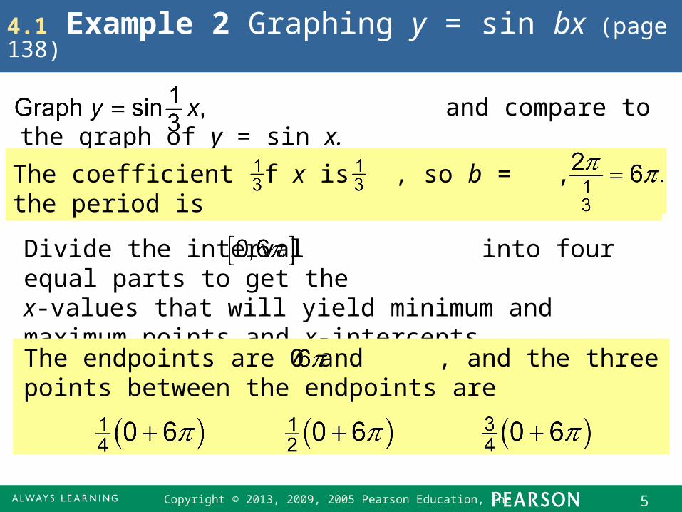
and compare to the graph of y = sin x.
4.1 Example 2 Graphing y = sin bx (page 138)
The coefficient of x is , so b = , and the period is
Divide the interval into four equal parts to get the x-values that will yield minimum and maximum points and x-intercepts.
The endpoints are 0 and , and the three points between the endpoints are
Copyright © 2013, 2009, 2005 Pearson Education, Inc. 6
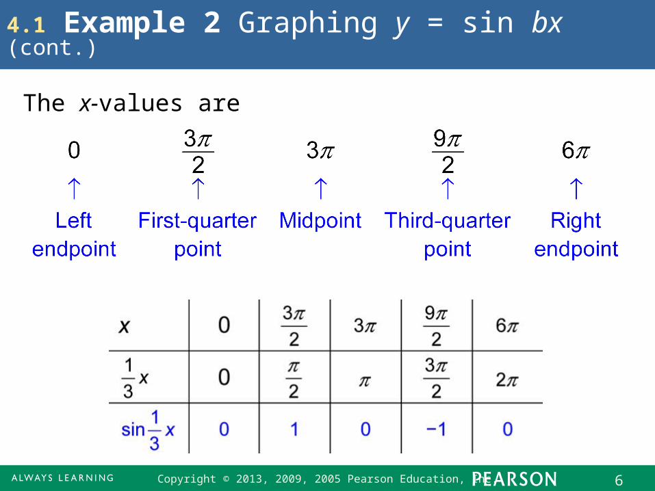
4.1 Example 2 Graphing y = sin bx (cont.)
The x-values are
Copyright © 2013, 2009, 2005 Pearson Education, Inc. 7
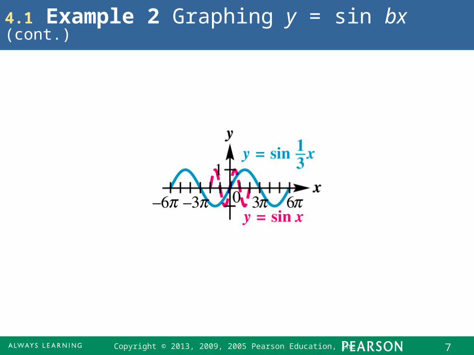
4.1 Example 2 Graphing y = sin bx (cont.)
Copyright © 2013, 2009, 2005 Pearson Education, Inc. 8
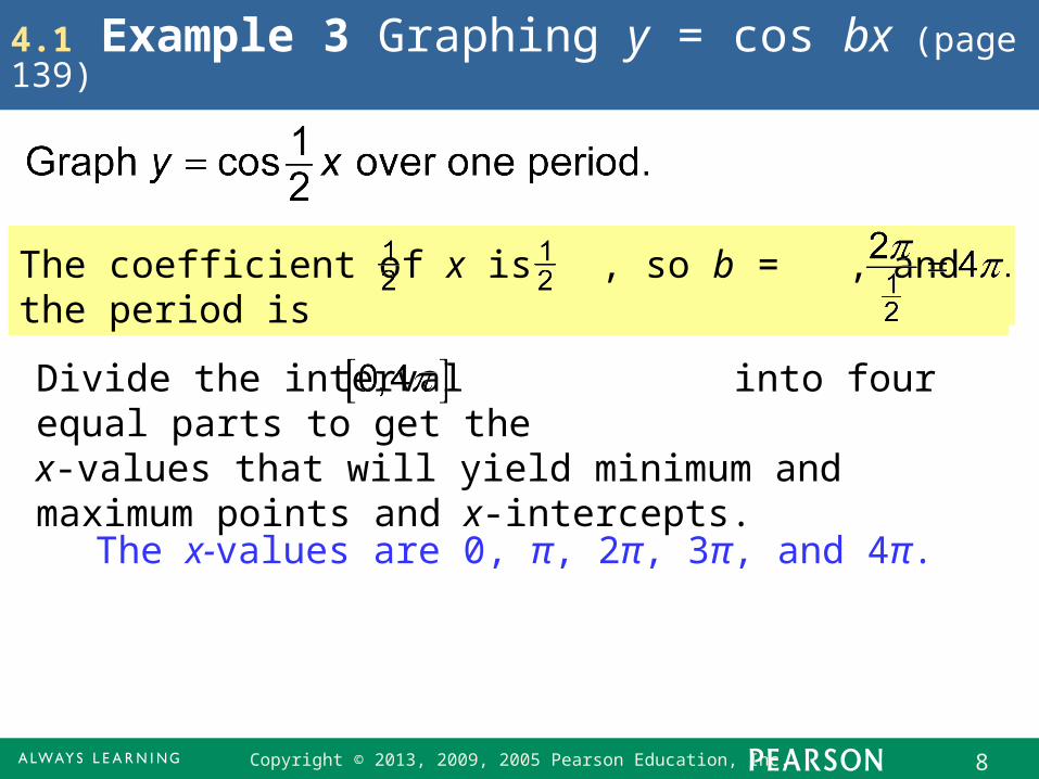
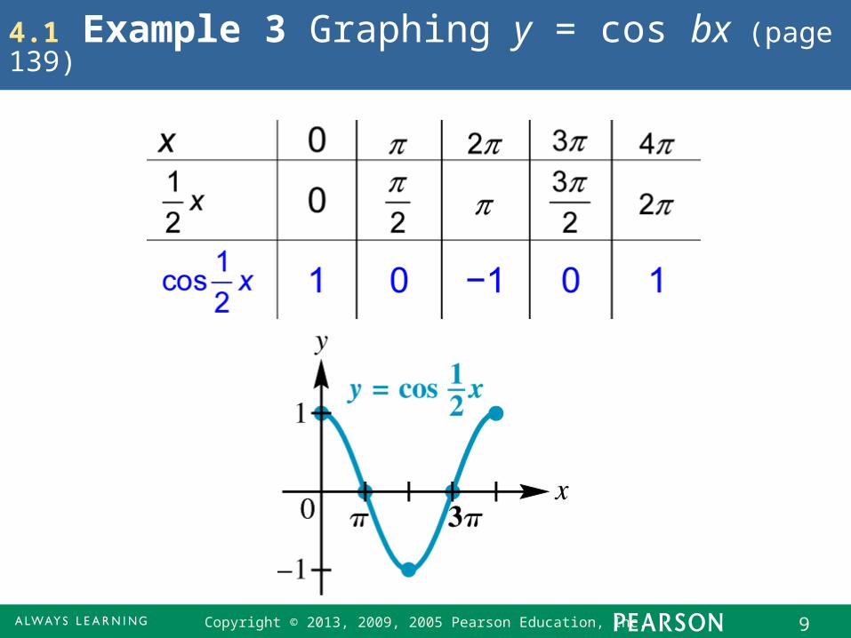
4.1 Example 3 Graphing y = cos bx (page 139)
The coefficient of x is , so b = , and the period is
Divide the interval into four equal parts to get the x-values that will yield minimum and maximum points and x-intercepts.
The x-values are 0, π, 2π, 3π, and 4π.
Copyright © 2013, 2009, 2005 Pearson Education, Inc. 9
4.1 Example 3 Graphing y = cos bx (page 139)
Copyright © 2013, 2009, 2005 Pearson Education, Inc. 10
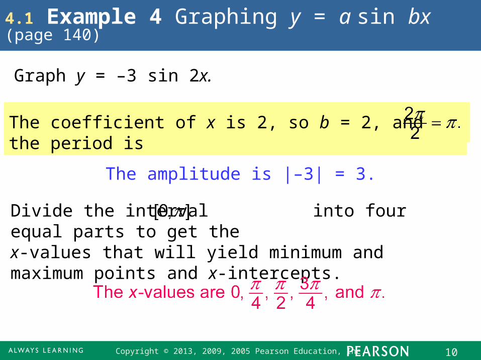
Graph y = –3 sin 2x.
4.1 Example 4 Graphing y = a sin bx (page 140)
The coefficient of x is 2, so b = 2, and the period is
The amplitude is |–3| = 3.
Divide the interval into four equal parts to get the x-values that will yield minimum and maximum points and x-intercepts.
Copyright © 2013, 2009, 2005 Pearson Education, Inc. 11
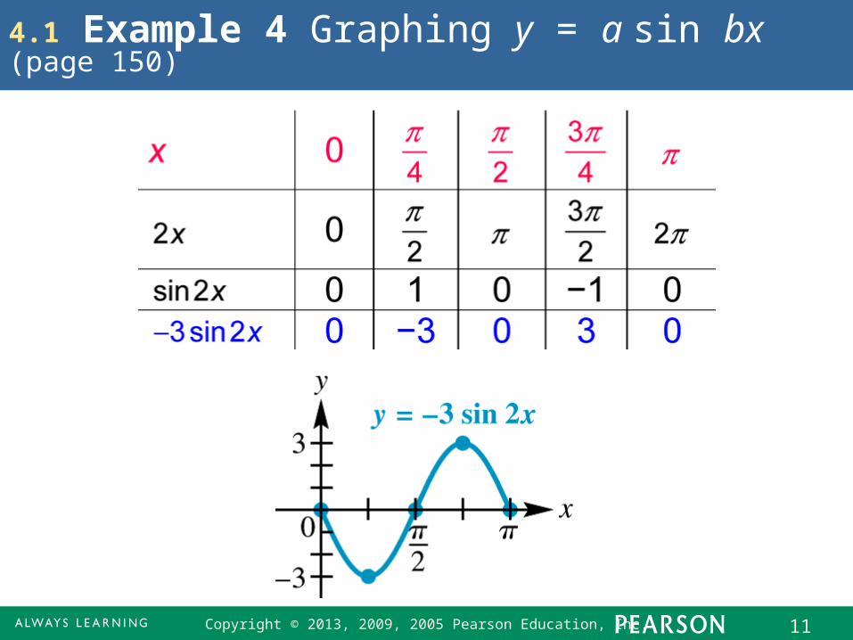
4.1 Example 4 Graphing y = a sin bx (page 150)
Copyright © 2013, 2009, 2005 Pearson Education, Inc. 12
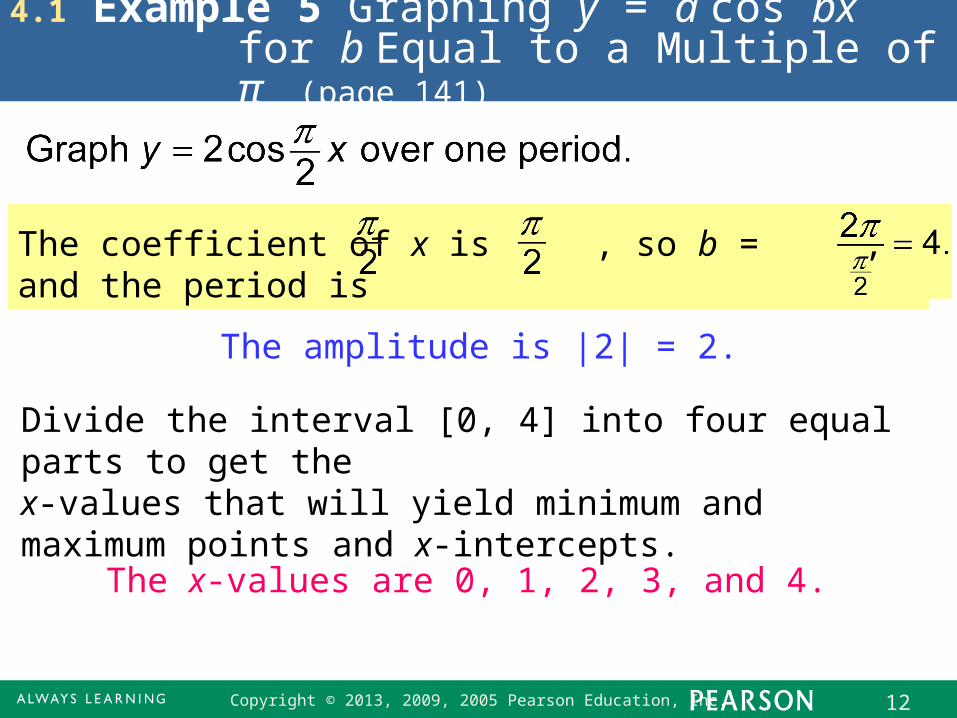
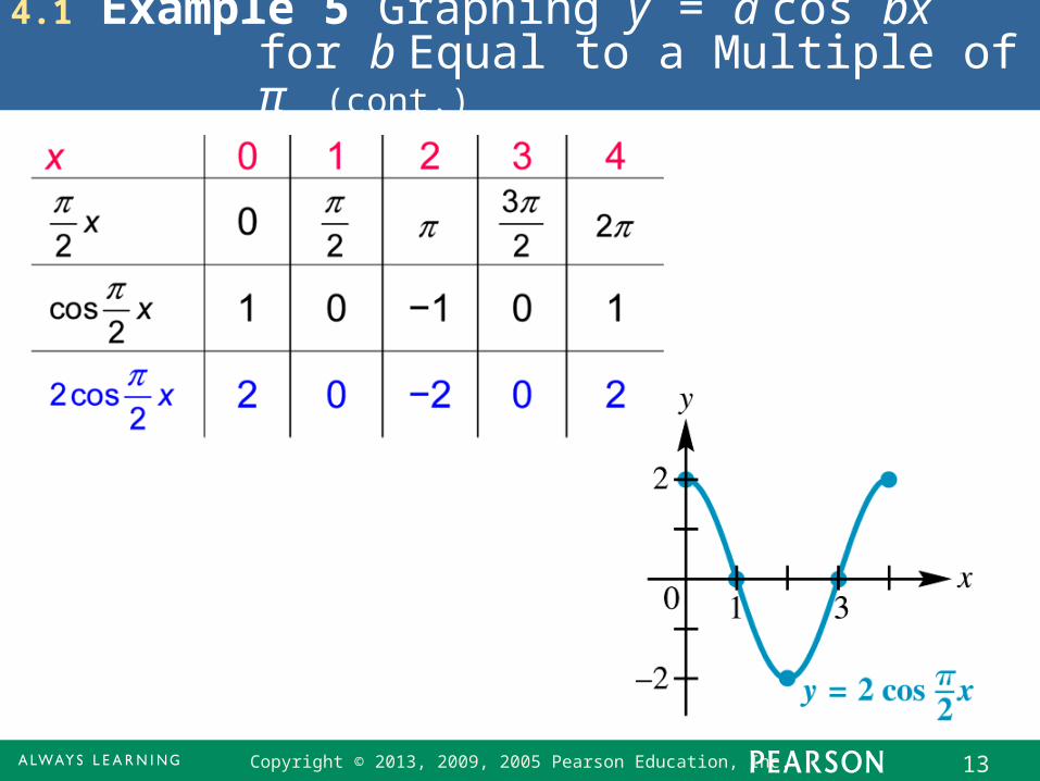
4.1 Example 5 Graphing y = a cos bx for b Equal to a Multiple of π (page 141)
The amplitude is |2| = 2.
Divide the interval [0, 4] into four equal parts to get the x-values that will yield minimum and maximum points and x-intercepts.
The coefficient of x is , so b = , and the period is
The x-values are 0, 1, 2, 3, and 4.
Copyright © 2013, 2009, 2005 Pearson Education, Inc. 13
4.1 Example 5 Graphing y = a cos bx for b Equal to a Multiple of π (cont.)
Copyright © 2013, 2009, 2005 Pearson Education, Inc. 14
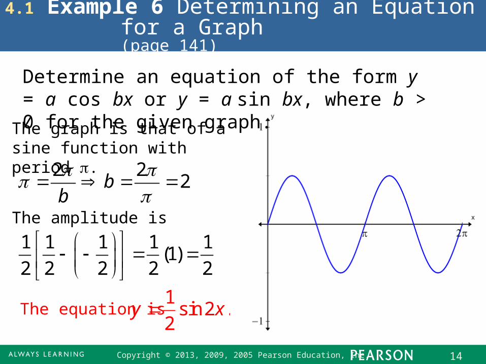
4.1 Example 6 Determining an Equation for a Graph (page 141)
Determine an equation of the form y = a cos bx or y = a sin bx, where b > 0 for the given graph.
The graph is that of a sine function with period .
2 22b
b
The amplitude is
1 1 1 1 1(1)
2 2 2 2 2
The equation is 1
sin2 .2
y x
Copyright © 2013, 2009, 2005 Pearson Education, Inc. 15
Translations of the Graphs of the Sine and Cosine Functions4.2Horizontal Translations ▪ Vertical Translations ▪ Combinations of Translations ▪ Determining a Trigonometric Model Using Curve Fitting
Copyright © 2013, 2009, 2005 Pearson Education, Inc. 16
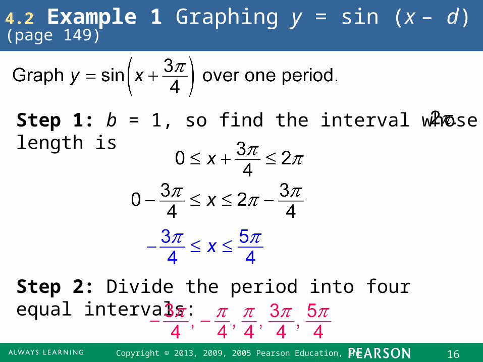
4.2 Example 1 Graphing y = sin (x – d) (page 149)
Step 2: Divide the period into four equal intervals:
Step 1: b = 1, so find the interval whose length is
Copyright © 2013, 2009, 2005 Pearson Education, Inc. 17
4.2 Example 1 Graphing y = sin (x – d) (cont.)
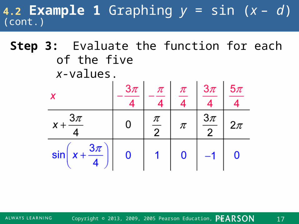
Step 3: Evaluate the function for each of the five x-values.
Copyright © 2013, 2009, 2005 Pearson Education, Inc. 18
4.2 Example 1 Graphing y = sin (x – d) (cont.)
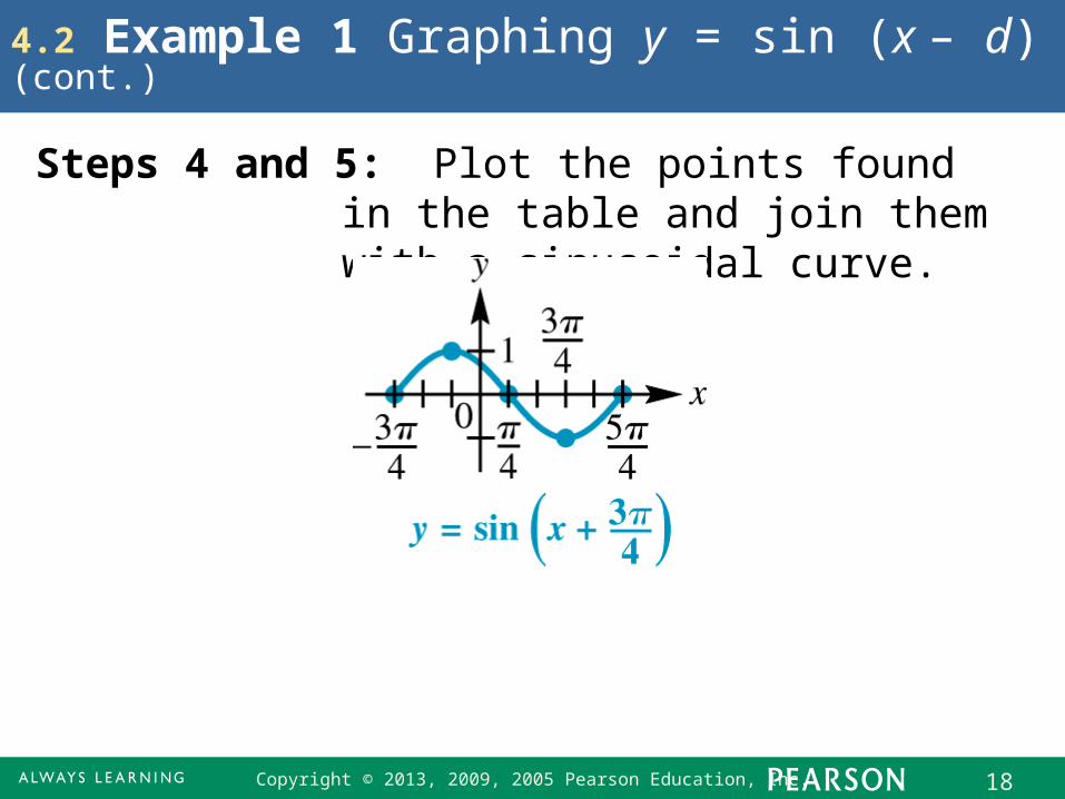
Steps 4 and 5: Plot the points found in the table and join them with a sinusoidal curve.
Copyright © 2013, 2009, 2005 Pearson Education, Inc. 19
4.2 Example 1 Graphing y = sin (x – d) (cont.)
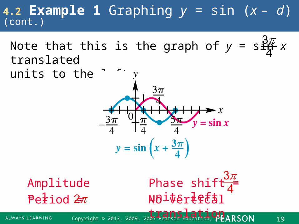
Note that this is the graph of y = sin x translated units to the left.
Amplitude = 1
Period =
Phase shift = units left
No vertical translation
Copyright © 2013, 2009, 2005 Pearson Education, Inc. 20
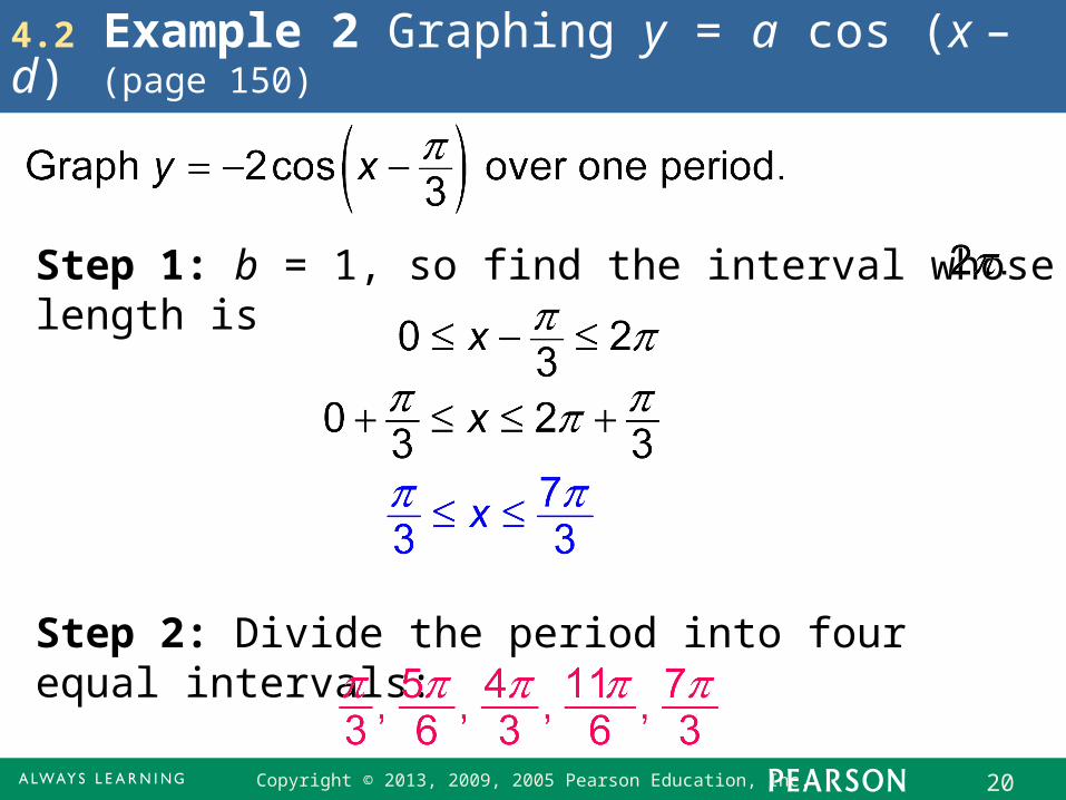
4.2 Example 2 Graphing y = a cos (x – d) (page 150)
Step 2: Divide the period into four equal intervals:
Step 1: b = 1, so find the interval whose length is
Copyright © 2013, 2009, 2005 Pearson Education, Inc. 21
4.2 Example 2 Graphing y = a cos (x – d) (cont.)
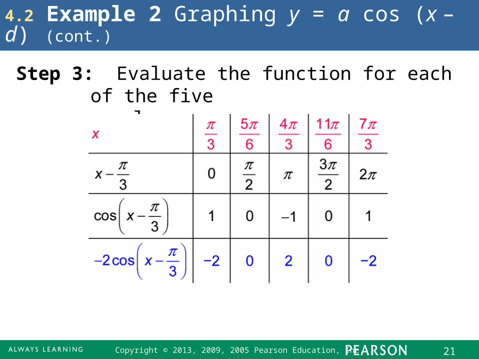
Step 3: Evaluate the function for each of the five x-values.
Copyright © 2013, 2009, 2005 Pearson Education, Inc. 22
4.2 Example 2 Graphing y = a cos (x – d) (cont.)
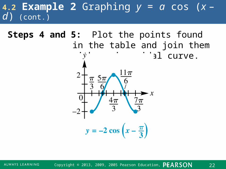
Steps 4 and 5: Plot the points found in the table and join them with a sinusoidal curve.
Copyright © 2013, 2009, 2005 Pearson Education, Inc. 23
4.2 Example 2 Graphing y = a cos (x – d) (cont.)
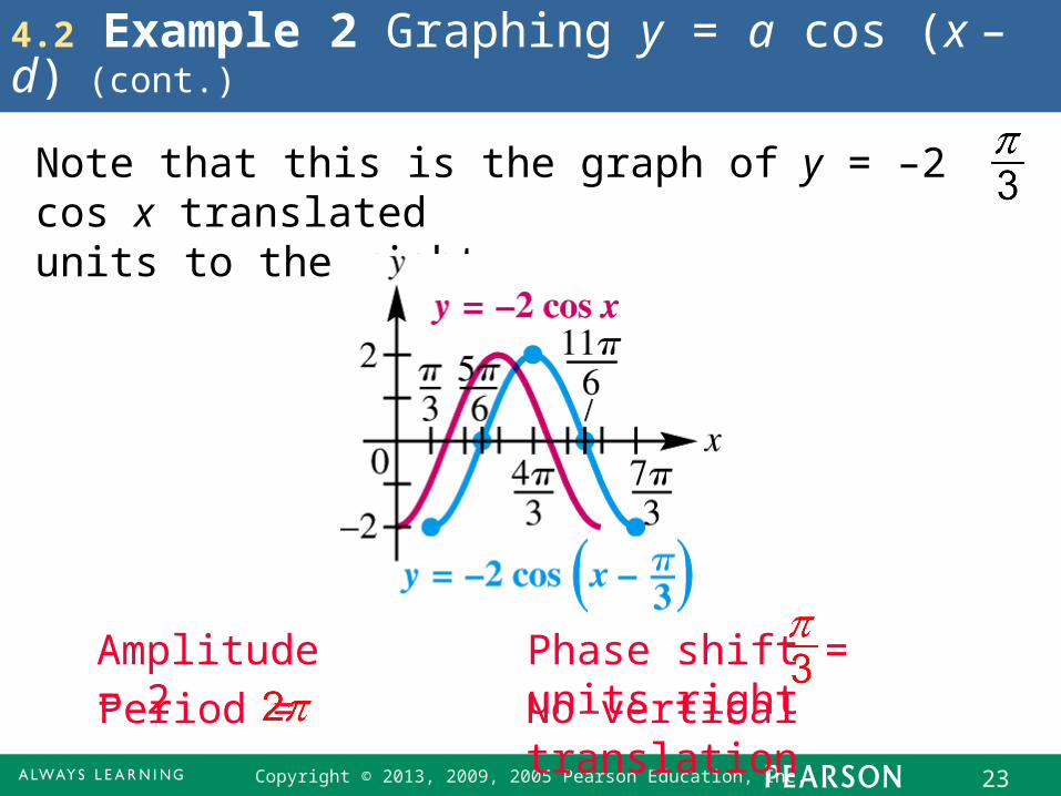
Note that this is the graph of y = –2 cos x translated units to the right.
Amplitude = 2
Period = No vertical translation
Phase shift = units right
Copyright © 2013, 2009, 2005 Pearson Education, Inc. 24
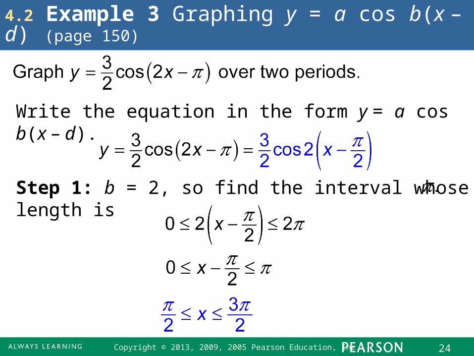
4.2 Example 3 Graphing y = a cos b(x – d) (page 150)
Write the equation in the form y = a cos b(x – d).
Step 1: b = 2, so find the interval whose length is
Copyright © 2013, 2009, 2005 Pearson Education, Inc. 25
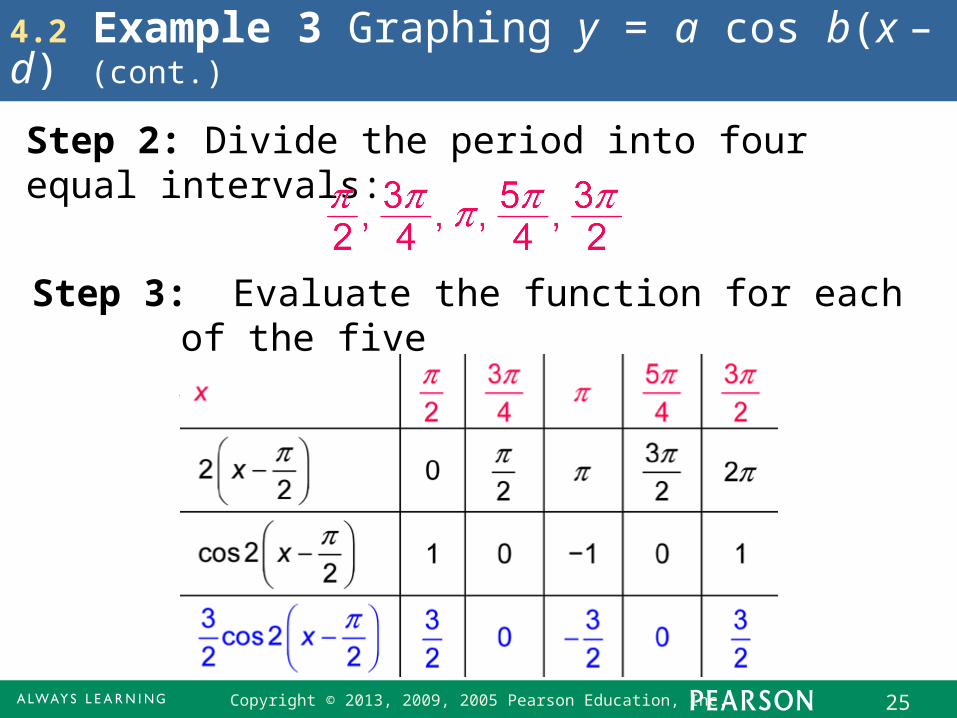
4.2 Example 3 Graphing y = a cos b(x – d) (cont.)
Step 2: Divide the period into four equal intervals:
Step 3: Evaluate the function for each of the five x-values.
Copyright © 2013, 2009, 2005 Pearson Education, Inc. 26
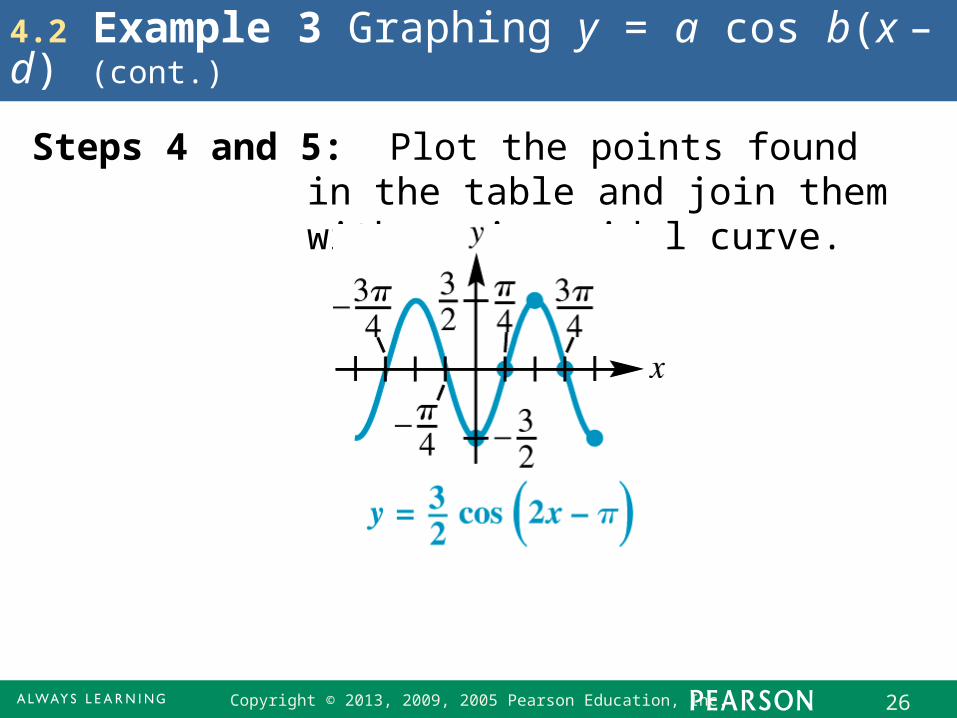
4.2 Example 3 Graphing y = a cos b(x – d) (cont.)
Steps 4 and 5: Plot the points found in the table and join them with a sinusoidal curve.
Copyright © 2013, 2009, 2005 Pearson Education, Inc. 27
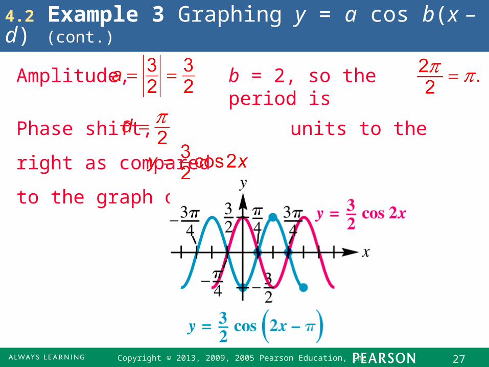
4.2 Example 3 Graphing y = a cos b(x – d) (cont.)
Amplitude, b = 2, so the period is
Phase shift, units to the right as compared
to the graph of
Copyright © 2013, 2009, 2005 Pearson Education, Inc. 28
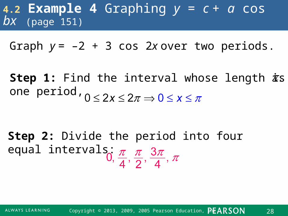
4.2 Example 4 Graphing y = c + a cos bx (page 151)
Step 1: Find the interval whose length is one period,
Graph y = –2 + 3 cos 2x over two periods.
Step 2: Divide the period into four equal intervals:
Copyright © 2013, 2009, 2005 Pearson Education, Inc. 29
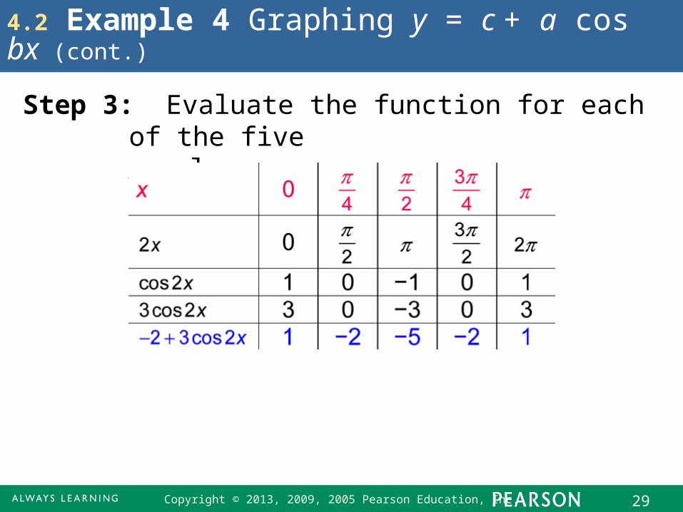
4.2 Example 4 Graphing y = c + a cos bx (cont.)
Step 3: Evaluate the function for each of the five x-values.
Copyright © 2013, 2009, 2005 Pearson Education, Inc. 30
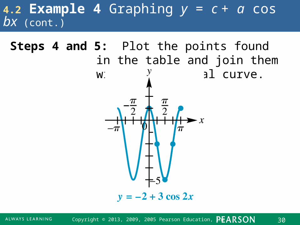
4.2 Example 4 Graphing y = c + a cos bx (cont.)
Steps 4 and 5: Plot the points found in the table and join them with a sinusoidal curve.
Copyright © 2013, 2009, 2005 Pearson Education, Inc. 31
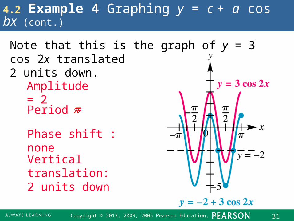
4.2 Example 4 Graphing y = c + a cos bx (cont.)
Note that this is the graph of y = 3 cos 2x translated 2 units down.
Amplitude = 2
Phase shift : none
Vertical translation: 2 units down
Period =
Copyright © 2013, 2009, 2005 Pearson Education, Inc. 32
Graphs of the Tangent and Cotangent Functions4.3Graph of the Tangent Function ▪ Graph of the Cotangent Function ▪ Graphing Techniques
Copyright © 2013, 2009, 2005 Pearson Education, Inc. 33
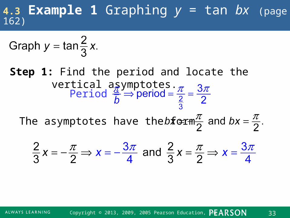
4.3 Example 1 Graphing y = tan bx (page 162)
Step 1: Find the period and locate the vertical asymptotes.
Period =
The asymptotes have the form
Copyright © 2013, 2009, 2005 Pearson Education, Inc. 34
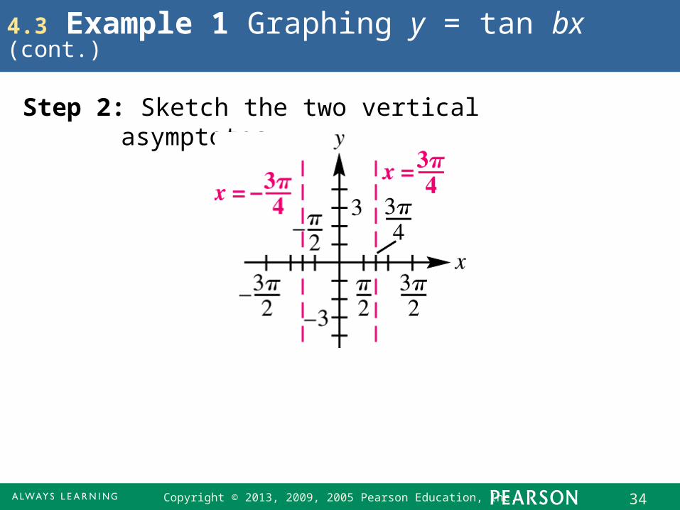
4.3 Example 1 Graphing y = tan bx (cont.)
Step 2: Sketch the two vertical asymptotes.
Copyright © 2013, 2009, 2005 Pearson Education, Inc. 35
4.3 Example 1 Graphing y = tan bx (cont.)
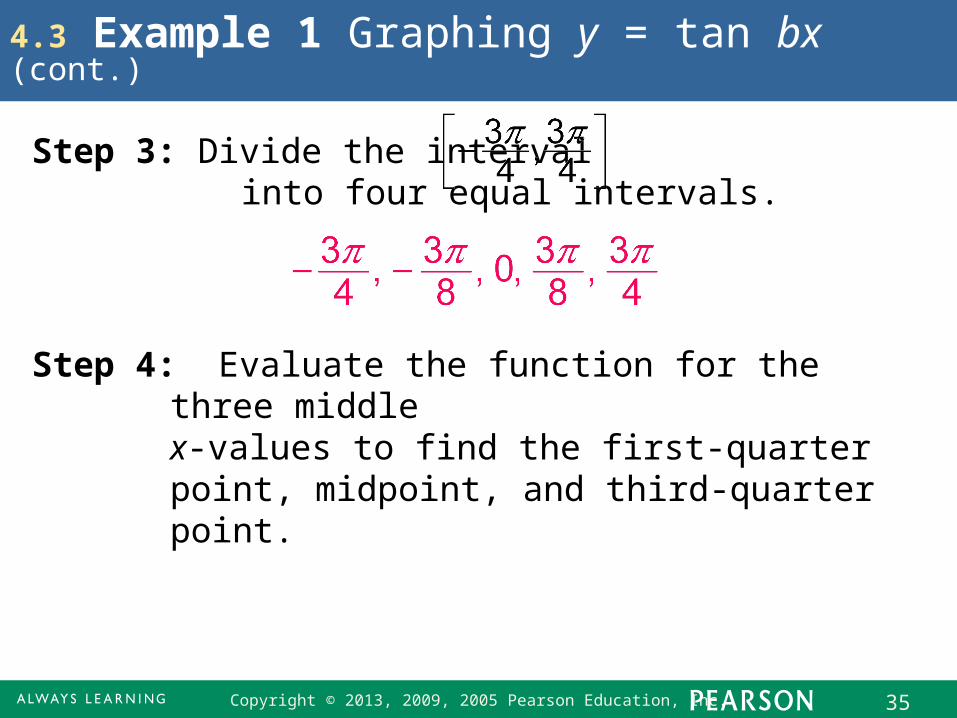
Step 3: Divide the interval into four equal intervals.
Step 4: Evaluate the function for the three middle x-values to find the first-quarter point, midpoint, and third-quarter point.
Copyright © 2013, 2009, 2005 Pearson Education, Inc. 36
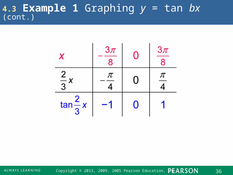
4.3 Example 1 Graphing y = tan bx (cont.)
Copyright © 2013, 2009, 2005 Pearson Education, Inc. 37
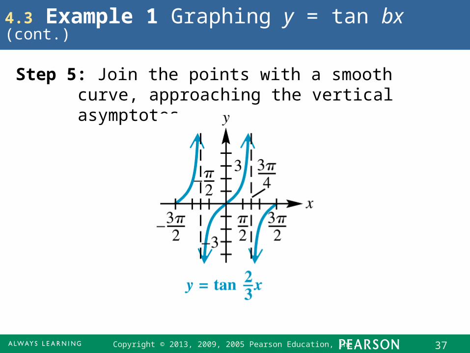
4.3 Example 1 Graphing y = tan bx (cont.)
Step 5: Join the points with a smooth curve, approaching the vertical asymptotes.
Copyright © 2013, 2009, 2005 Pearson Education, Inc. 38
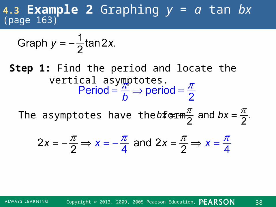
4.3 Example 2 Graphing y = a tan bx (page 163)
Step 1: Find the period and locate the vertical asymptotes.
The asymptotes have the form
Copyright © 2013, 2009, 2005 Pearson Education, Inc. 39
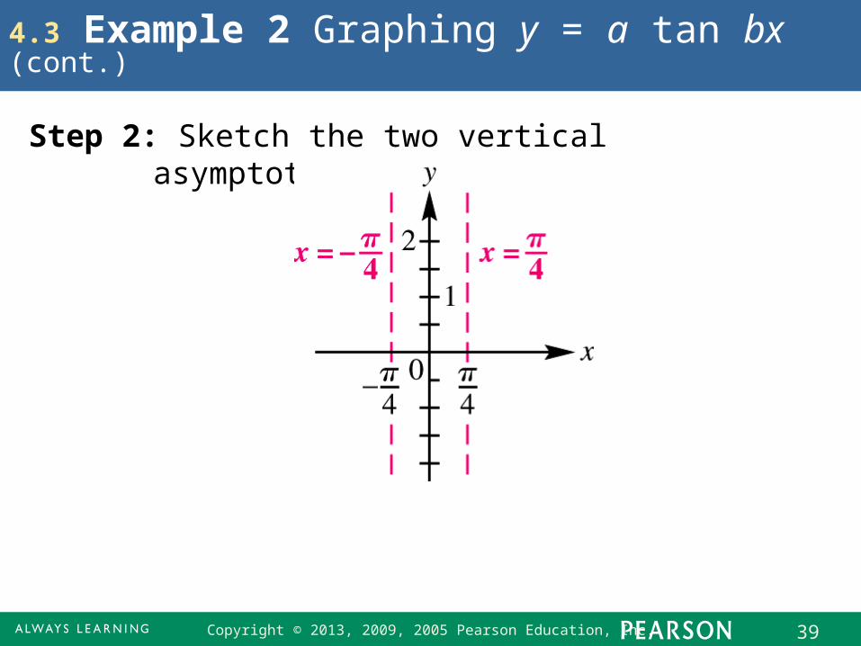
4.3 Example 2 Graphing y = a tan bx (cont.)
Step 2: Sketch the two vertical asymptotes.
Copyright © 2013, 2009, 2005 Pearson Education, Inc. 40
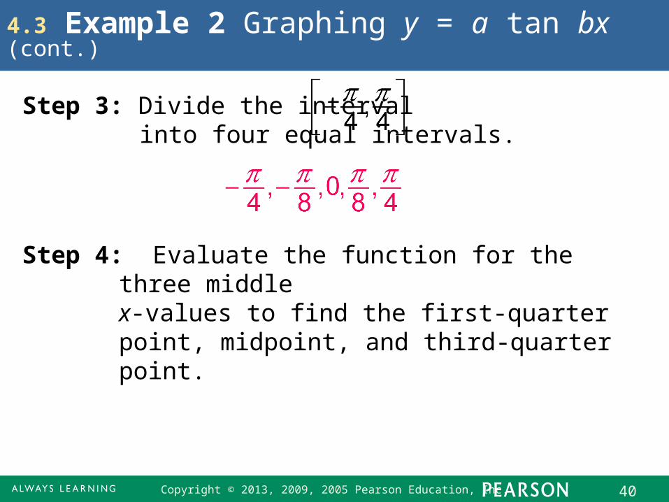
4.3 Example 2 Graphing y = a tan bx (cont.)
Step 3: Divide the interval into four equal intervals.
Step 4: Evaluate the function for the three middle x-values to find the first-quarter point, midpoint, and third-quarter point.
Copyright © 2013, 2009, 2005 Pearson Education, Inc. 41
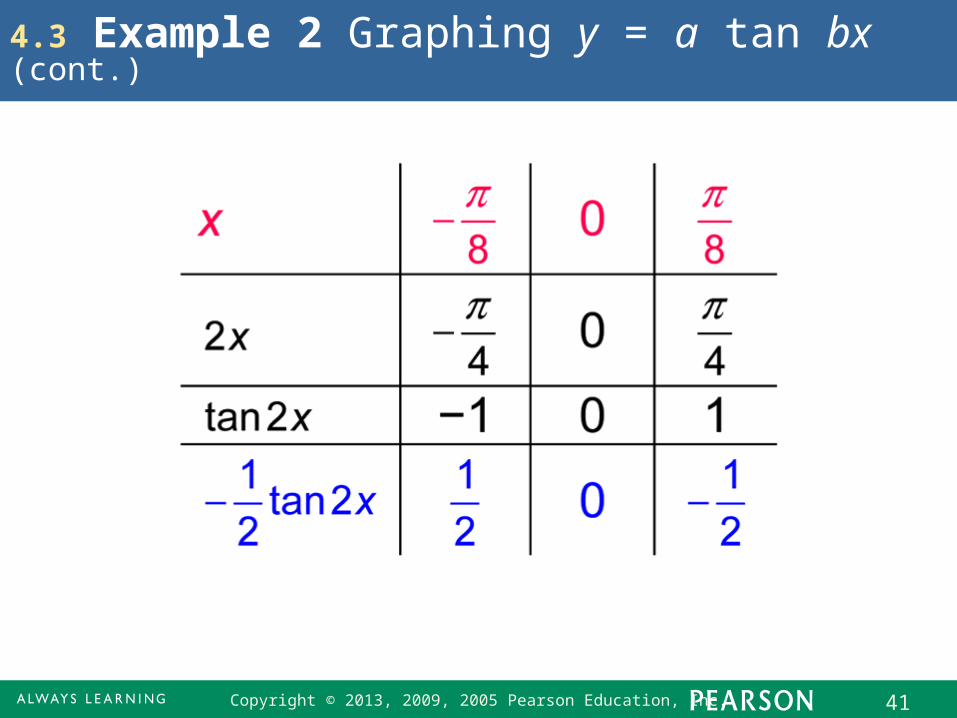
4.3 Example 2 Graphing y = a tan bx (cont.)
Copyright © 2013, 2009, 2005 Pearson Education, Inc. 42
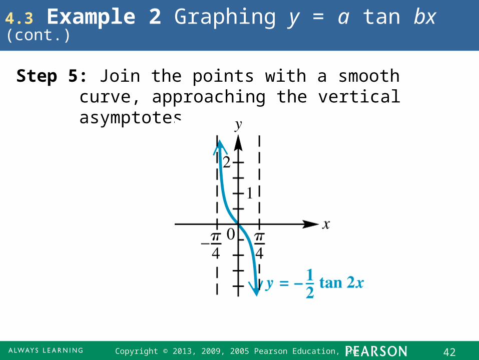
4.3 Example 2 Graphing y = a tan bx (cont.)
Step 5: Join the points with a smooth curve, approaching the vertical asymptotes.
Copyright © 2013, 2009, 2005 Pearson Education, Inc. 43
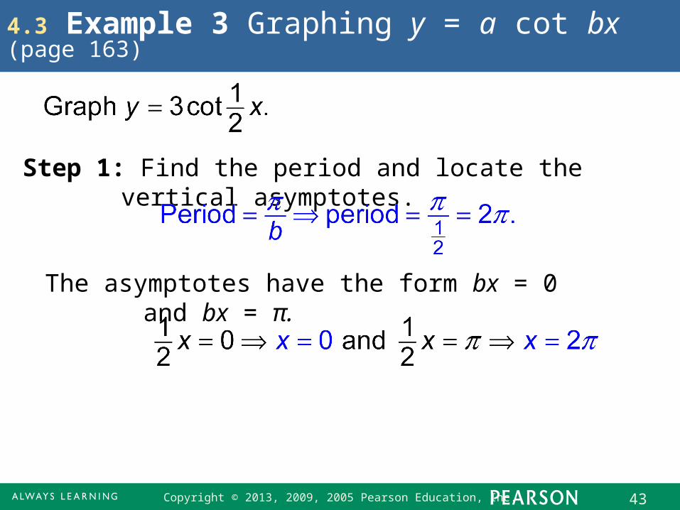
4.3 Example 3 Graphing y = a cot bx (page 163)
Step 1: Find the period and locate the vertical asymptotes.
The asymptotes have the form bx = 0 and bx = π.
Copyright © 2013, 2009, 2005 Pearson Education, Inc. 44
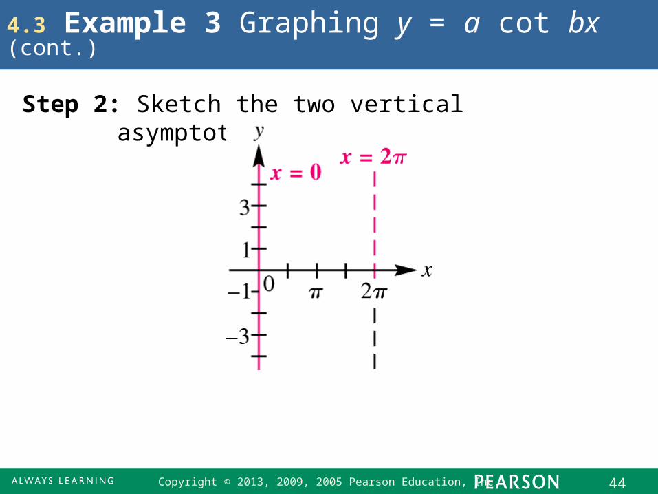
4.3 Example 3 Graphing y = a cot bx (cont.)
Step 2: Sketch the two vertical asymptotes.
Copyright © 2013, 2009, 2005 Pearson Education, Inc. 45
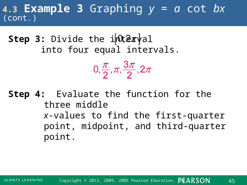
4.3 Example 3 Graphing y = a cot bx (cont.)
Step 3: Divide the interval into four equal intervals.
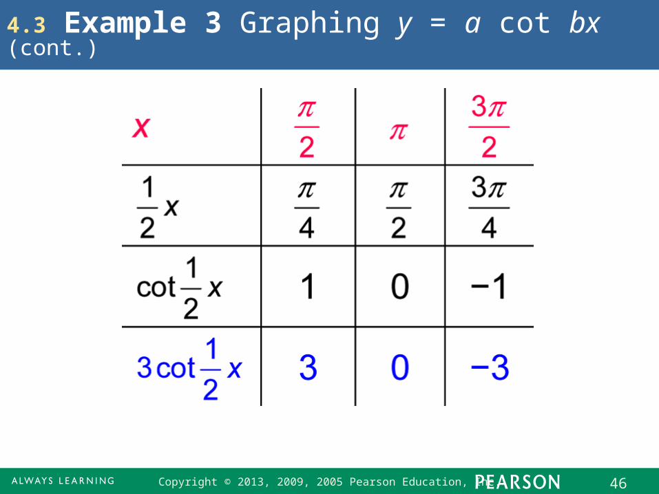
Step 4: Evaluate the function for the three middle x-values to find the first-quarter point, midpoint, and third-quarter point.
Copyright © 2013, 2009, 2005 Pearson Education, Inc. 46
4.3 Example 3 Graphing y = a cot bx (cont.)
Copyright © 2013, 2009, 2005 Pearson Education, Inc. 47
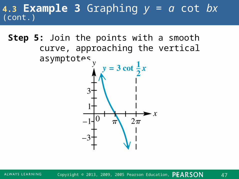
4.3 Example 3 Graphing y = a cot bx (cont.)
Step 5: Join the points with a smooth curve, approaching the vertical asymptotes.
Copyright © 2013, 2009, 2005 Pearson Education, Inc. 48
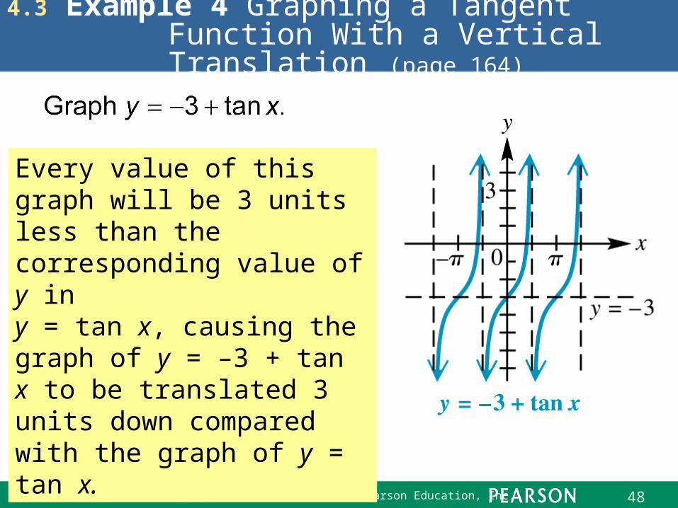
4.3 Example 4 Graphing a Tangent Function With a Vertical Translation (page 164)
Every value of this graph will be 3 units less than the corresponding value of y in y = tan x, causing the graph of y = –3 + tan x to be translated 3 units down compared with the graph of y = tan x.
Copyright © 2013, 2009, 2005 Pearson Education, Inc. 49
Graphs of the Secant and Cosecant Functions4.4Graph of the Secant Function ▪ Graph of the Cosecant Function ▪ Graphing Techniques ▪ Addition of Ordinates ▪ Connecting Graphs with Equations
Copyright © 2013, 2009, 2005 Pearson Education, Inc. 50
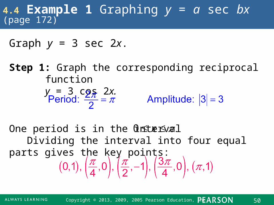
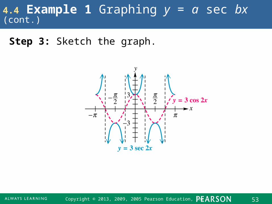
4.4 Example 1 Graphing y = a sec bx (page 172)
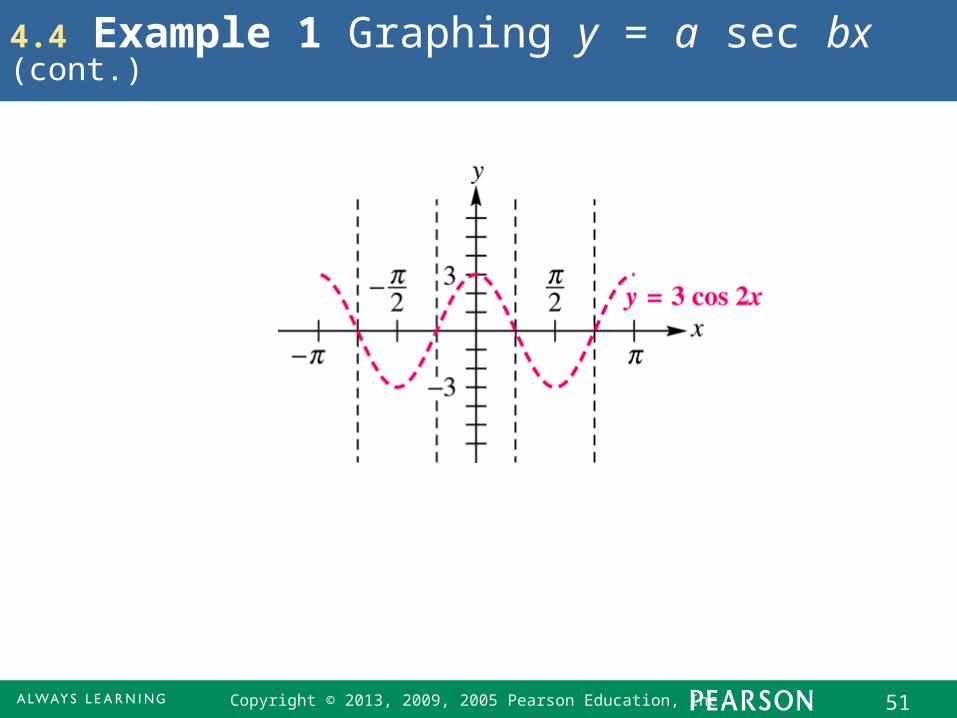
Step 1: Graph the corresponding reciprocal functiony = 3 cos 2x.
Graph y = 3 sec 2x.
One period is in the interval Dividing the interval into four equal parts gives the key points:
Copyright © 2013, 2009, 2005 Pearson Education, Inc. 51
4.4 Example 1 Graphing y = a sec bx (cont.)
Copyright © 2013, 2009, 2005 Pearson Education, Inc. 52
4.4 Example 1 Graphing y = a sec bx (cont.)
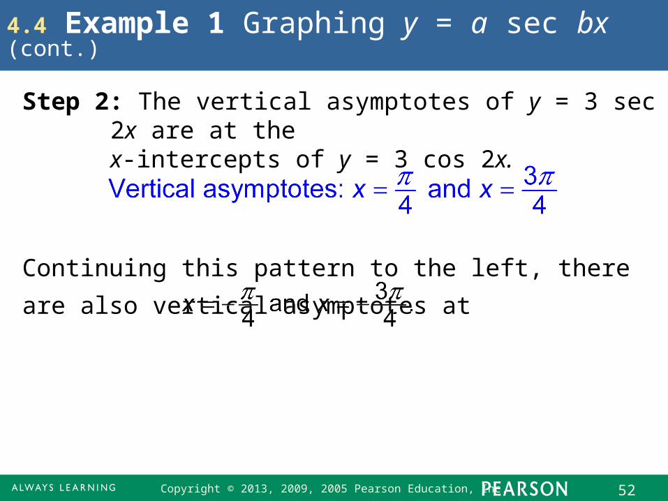
Step 2: The vertical asymptotes of y = 3 sec 2x are at the x-intercepts of y = 3 cos 2x.
Continuing this pattern to the left, there are also vertical
asymptotes at
Copyright © 2013, 2009, 2005 Pearson Education, Inc. 53
4.4 Example 1 Graphing y = a sec bx (cont.)
Step 3: Sketch the graph.
Copyright © 2013, 2009, 2005 Pearson Education, Inc. 54
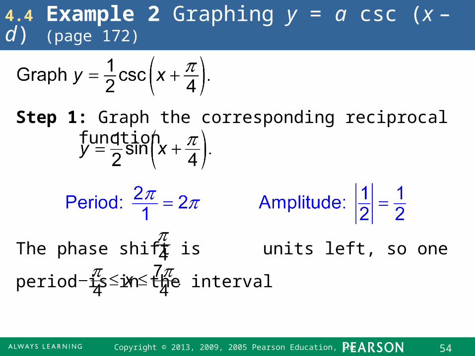
4.4 Example 2 Graphing y = a csc (x – d) (page 172)
Step 1: Graph the corresponding reciprocal function
The phase shift is units left, so one period is in the
interval
Copyright © 2013, 2009, 2005 Pearson Education, Inc. 55
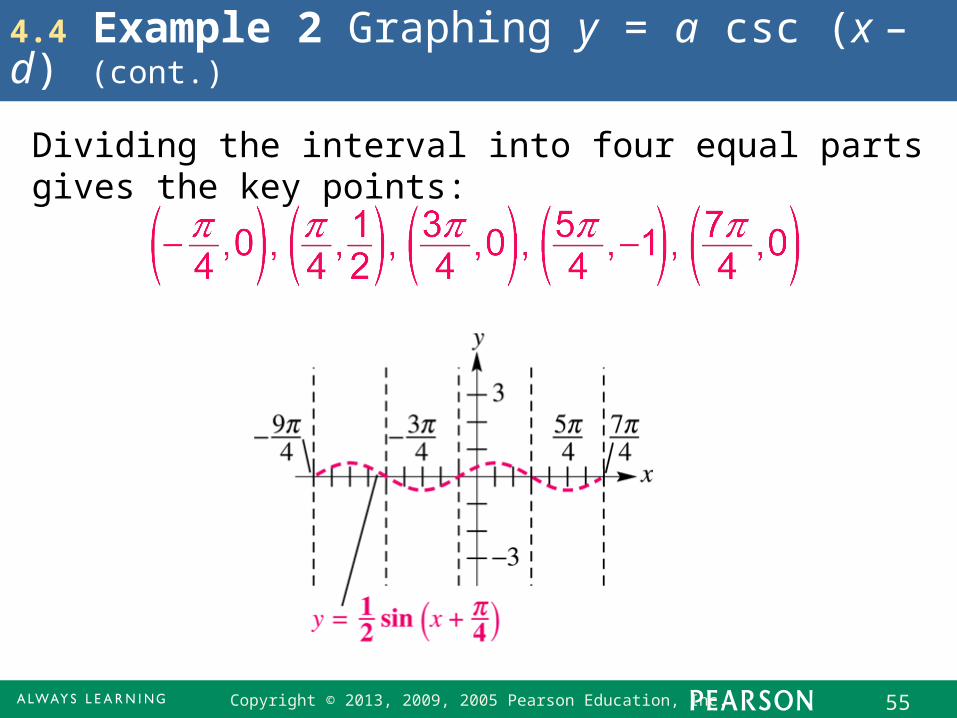
4.4 Example 2 Graphing y = a csc (x – d) (cont.)
Dividing the interval into four equal parts gives the key points:
Copyright © 2013, 2009, 2005 Pearson Education, Inc. 56
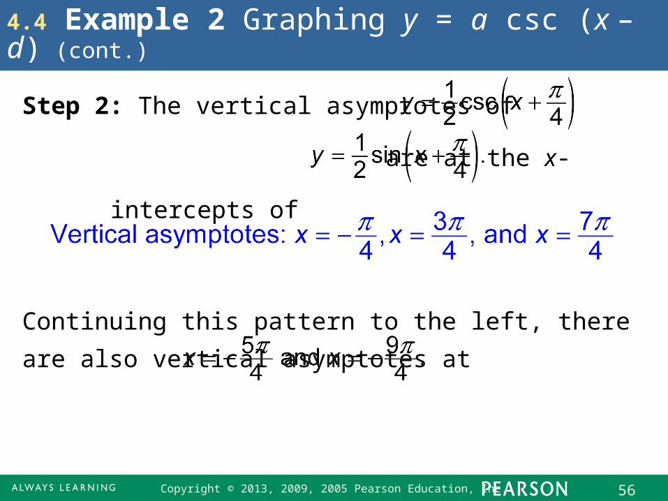
4.4 Example 2 Graphing y = a csc (x – d) (cont.)
Step 2: The vertical asymptotes of are at
the x-intercepts of
Continuing this pattern to the left, there are also vertical
asymptotes at
Copyright © 2013, 2009, 2005 Pearson Education, Inc. 57
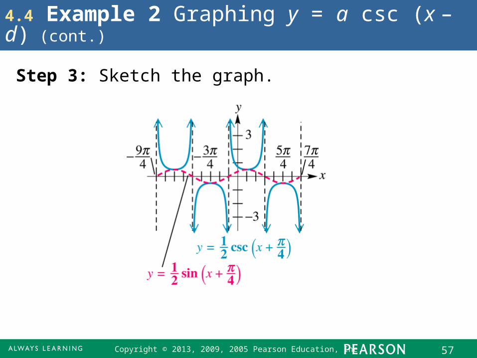
4.4 Example 2 Graphing y = a csc (x – d) (cont.)
Step 3: Sketch the graph.
Copyright © 2013, 2009, 2005 Pearson Education, Inc. 58
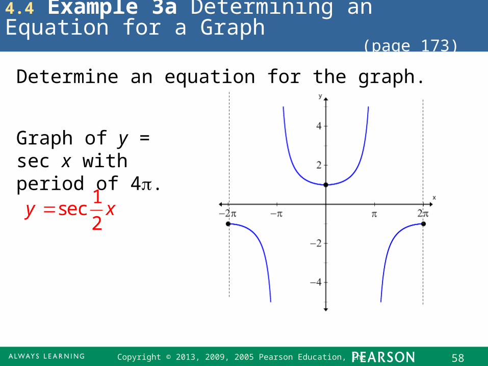
4.4 Example 3a Determining an Equation for a Graph (page 173)
Determine an equation for the graph.
1sec
2y x
Graph of y = sec x with period of 4.
Copyright © 2013, 2009, 2005 Pearson Education, Inc. 59
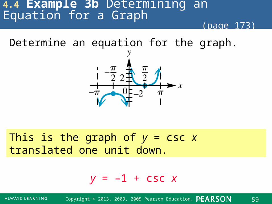
4.4 Example 3b Determining an Equation for a Graph (page 173)
Determine an equation for the graph.
This is the graph of y = csc x translated one unit down.
y = –1 + csc x