Copyright ©2011 Pearson Education 7-1 Chapter 7 Sampling and Sampling Distributions Statistics for Managers using Microsoft Excel 6 th Global Edition

Copyright ©2011 Pearson Education7-1

Chapter 7

Sampling and Sampling Distributions

Statistics for Managers using Microsoft Excel6th Global Edition


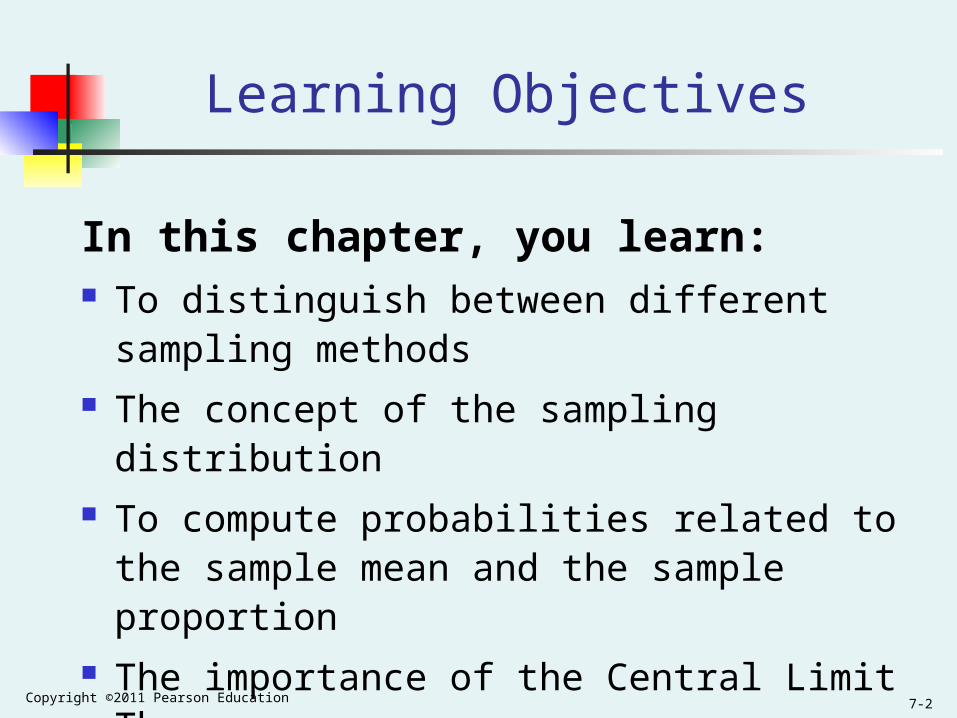
Learning Objectives

In this chapter, you learn: To distinguish between different sampling

methods The concept of the sampling distribution To compute probabilities related to the sample

mean and the sample proportion The importance of the Central Limit Theorem


Why Sample?

Selecting a sample is less time-consuming than selecting every item in the population (census).

An analysis of a sample is less cumbersome and more practical than an analysis of the entire population.

DCOVA


A Sampling Process Begins With A Sampling Frame

The sampling frame is a listing of items that make up the population

Frames are data sources such as population lists, directories, or maps

Inaccurate or biased results can result if a frame excludes certain portions of the population

Using different frames to generate data can lead to dissimilar conclusions

DCOVA


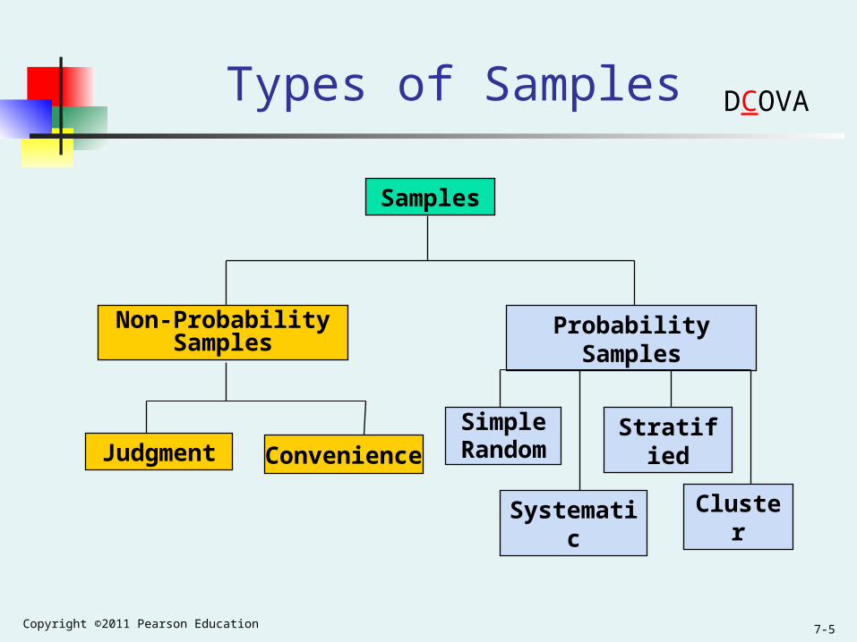
Types of Samples

Samples

Non-Probability Samples

Judgment

Probability Samples

Simple Random

Systematic

Stratified

Cluster

Convenience

DCOVA


Types of Samples:Nonprobability Sample

In a nonprobability sample, items included are chosen without regard to their probability of occurrence. In convenience sampling, items are selected based

only on the fact that they are easy, inexpensive, or convenient to sample.

In a judgment sample, you get the opinions of pre-selected experts in the subject matter.

DCOVA


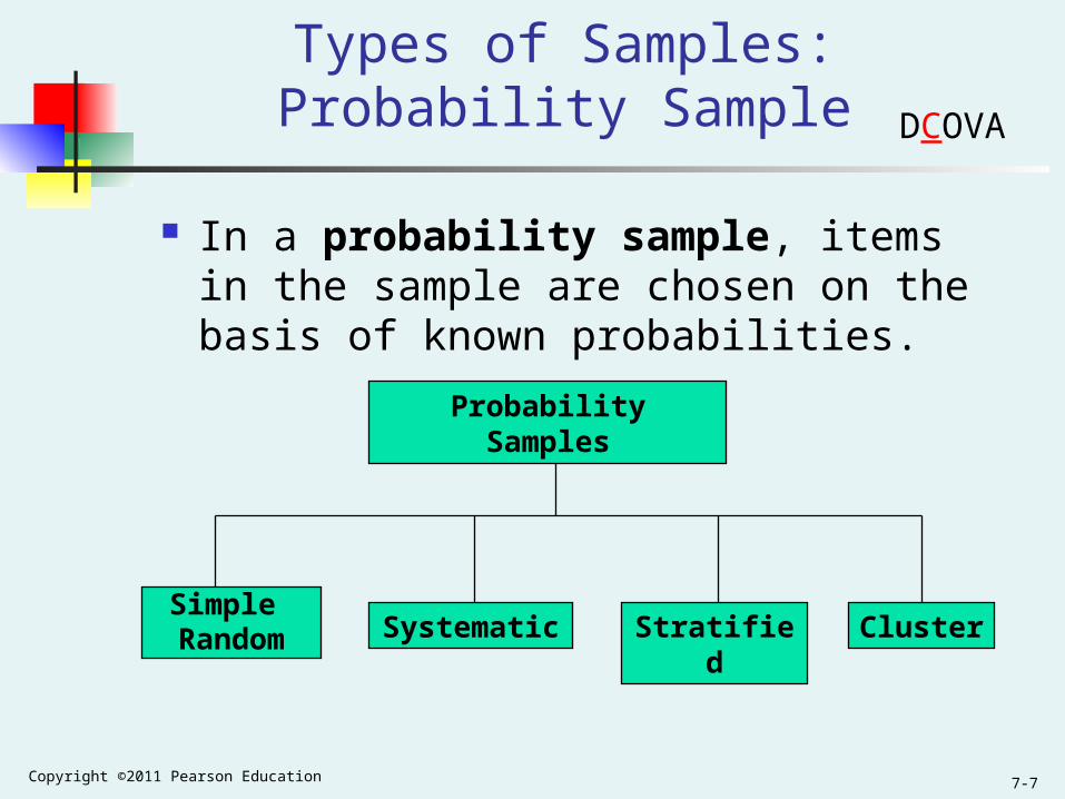
Types of Samples:Probability Sample

In a probability sample, items in the sample are chosen on the basis of known probabilities.

Probability Samples

Simple Random Systematic Stratified Cluster

DCOVA


Probability Sample:Simple Random Sample

Every individual or item from the frame has an equal chance of being selected

Selection may be with replacement (selected individual is returned to frame for possible reselection) or without replacement (selected individual isn’t returned to the frame).

Samples obtained from table of random numbers or computer random number generators.

DCOVA


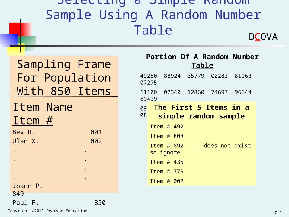
Selecting a Simple Random Sample Using A Random Number Table

Sampling Frame For Population With 850

Items

Item Name Item #Bev R. 001

Ulan X. 002

. .

. .

. .

. .

Joann P. 849

Paul F. 850

Portion Of A Random Number Table49280 88924 35779 00283 81163 07275

11100 02340 12860 74697 96644 89439

09893 23997 20048 49420 88872 08401

The First 5 Items in a simple random sample

Item # 492

Item # 808

Item # 892 -- does not exist so ignore

Item # 435

Item # 779

Item # 002

DCOVA


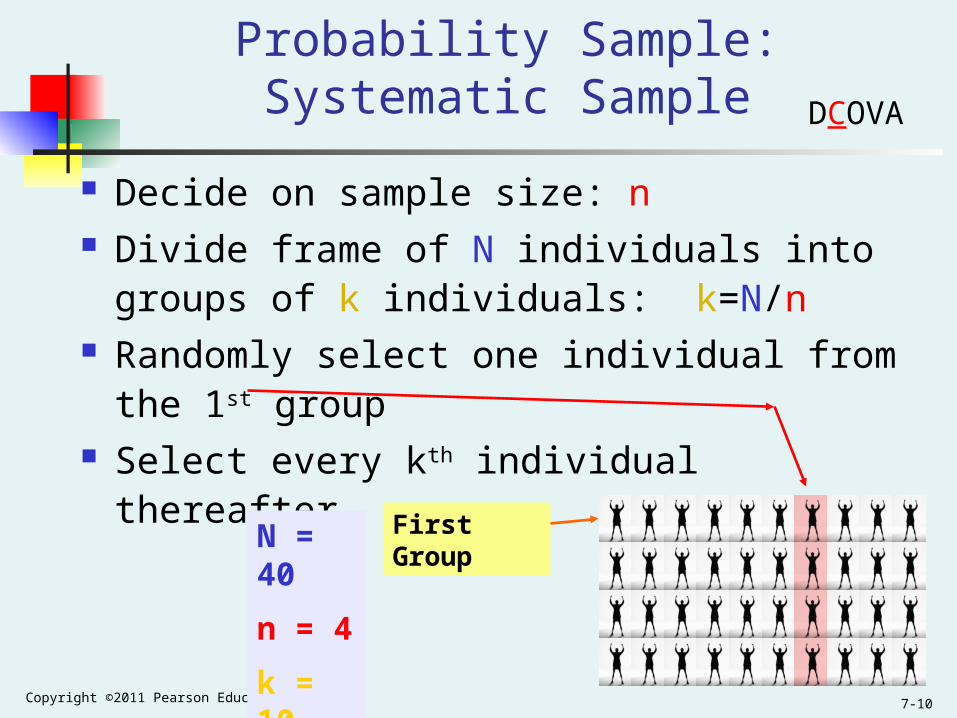
Decide on sample size: n Divide frame of N individuals into groups of k

individuals: k=N/n Randomly select one individual from the 1st

group Select every kth individual thereafter

Probability Sample:Systematic Sample

N = 40

n = 4

k = 10

First Group

DCOVA


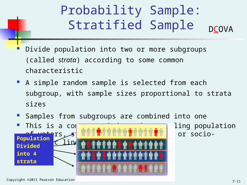
Probability Sample:Stratified Sample

Divide population into two or more subgroups (called strata)

according to some common characteristic

A simple random sample is selected from each subgroup, with sample

sizes proportional to strata sizes

Samples from subgroups are combined into one This is a common technique when sampling population of voters,

stratifying across racial or socio-economic lines.

Population

Divided

into 4

strata

DCOVA


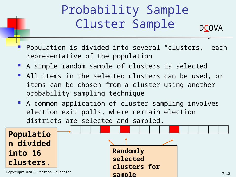
Probability SampleCluster Sample

Population is divided into several “clusters,” each representative of the population

A simple random sample of clusters is selected All items in the selected clusters can be used, or items can be

chosen from a cluster using another probability sampling technique A common application of cluster sampling involves election exit polls,

where certain election districts are selected and sampled.

Population divided into 16 clusters. Randomly selected

clusters for sample

DCOVA


Probability Sample:Comparing Sampling Methods

Simple random sample and Systematic sample Simple to use May not be a good representation of the population’s

underlying characteristics Stratified sample

Ensures representation of individuals across the entire population

Cluster sample More cost effective Less efficient (need larger sample to acquire the same

level of precision)

DCOVA


Evaluating Survey Worthiness

What is the purpose of the survey? Is the survey based on a probability sample? Coverage error – appropriate frame? Nonresponse error – follow up Measurement error – good questions elicit good

responses Sampling error – always exists

DCOVA


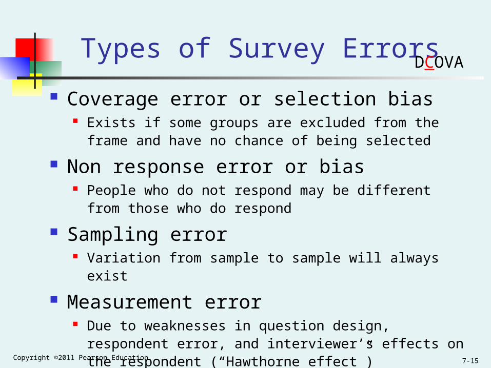
Types of Survey Errors

Coverage error or selection bias Exists if some groups are excluded from the frame and have

no chance of being selected

Non response error or bias People who do not respond may be different from those who

do respond

Sampling error Variation from sample to sample will always exist

Measurement error Due to weaknesses in question design, respondent error, and

interviewer’s effects on the respondent (“Hawthorne effect”)

DCOVA


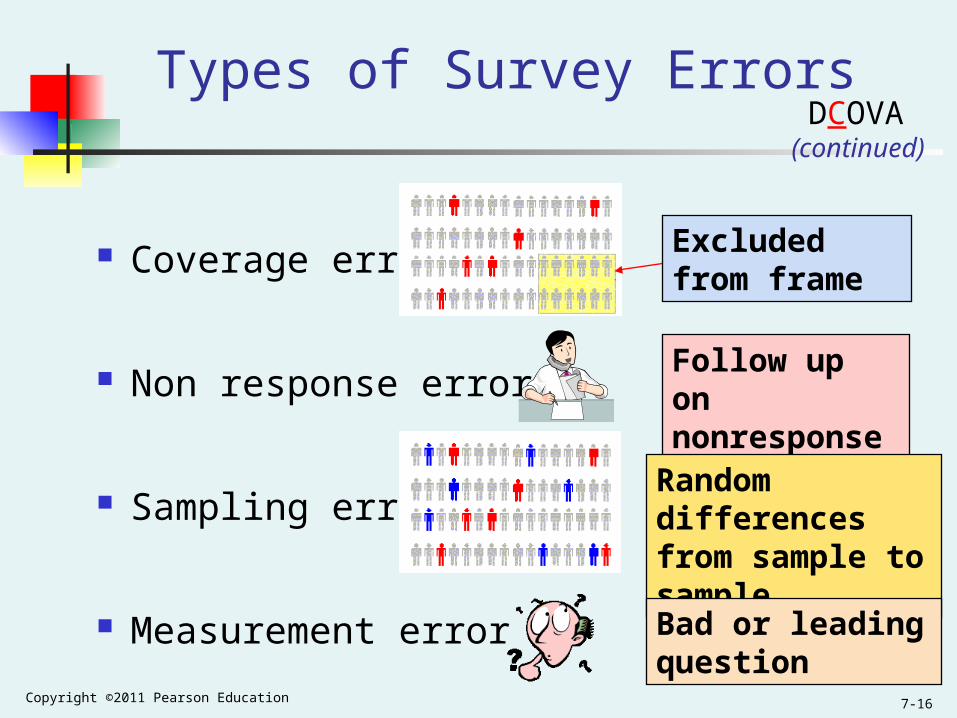
Types of Survey Errors

Coverage error

Non response error

Sampling error

Measurement error

Excluded from frame

Follow up on nonresponses

Random differences from sample to sample

Bad or leading question

(continued)DCOVA


Sampling Distributions

A sampling distribution is a distribution of all of the possible values of a sample statistic for a given size sample selected from a population.

For example, suppose you sample 50 students from your college regarding their mean GPA. If you obtained many different samples of 50, you will compute a different mean for each sample. We are interested in the distribution of all potential mean GPA we might calculate for any given sample of 50 students.

DCOVA


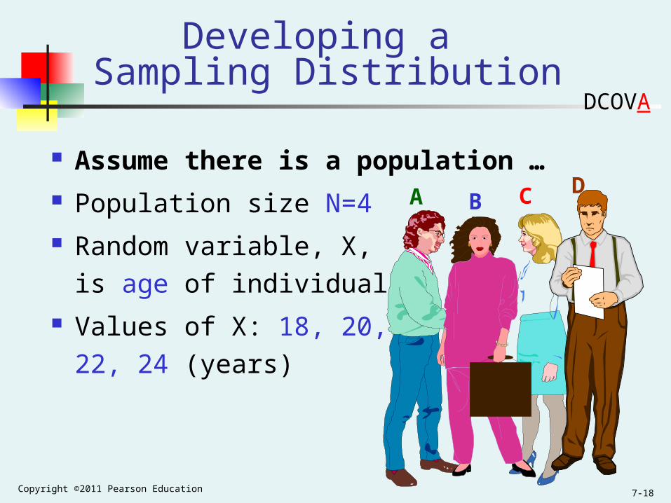
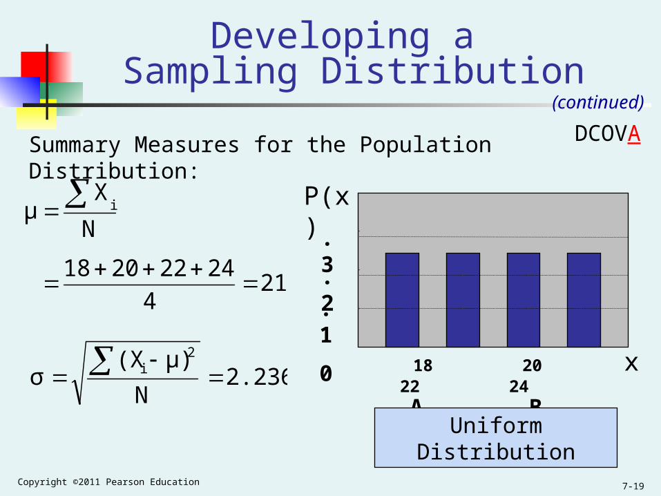
Developing a Sampling Distribution

Assume there is a population … Population size N=4 Random variable, X,

is age of individuals Values of X: 18, 20,

22, 24 (years)

A B C D

DCOVA


.3

.2

.1

0 18 20 22 24

A B C D

Uniform Distribution

P(x)

x

(continued)

Summary Measures for the Population Distribution:


214

24222018

N

Xμ i

2.236N

μ)(Xσ

2i

DCOVA


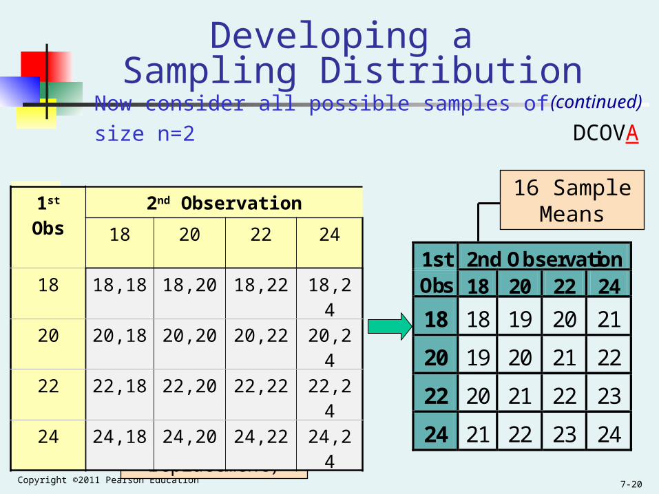
16 possible samples (sampling with replacement)

Now consider all possible samples of size n=2

1st 2nd Observation Obs 18 20 22 24

18 18 19 20 21

20 19 20 21 22

22 20 21 22 23

24 21 22 23 24

(continued)


16 Sample Means

1st

Obs2nd Observation

18 20 22 24

18 18,18 18,20 18,22 18,24

20 20,18 20,20 20,22 20,24

22 22,18 22,20 22,22 22,24

24 24,18 24,20 24,22 24,24

DCOVA


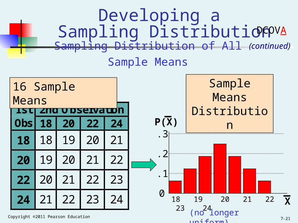
1st 2nd Observation Obs 18 20 22 24

18 18 19 20 21

20 19 20 21 22

22 20 21 22 23

24 21 22 23 24

Sampling Distribution of All Sample Means

18 19 20 21 22 23 240

.1

.2

.3 P(X)

X

Sample Means Distribution

16 Sample Means

_


(continued)

(no longer uniform)

_

DCOVA


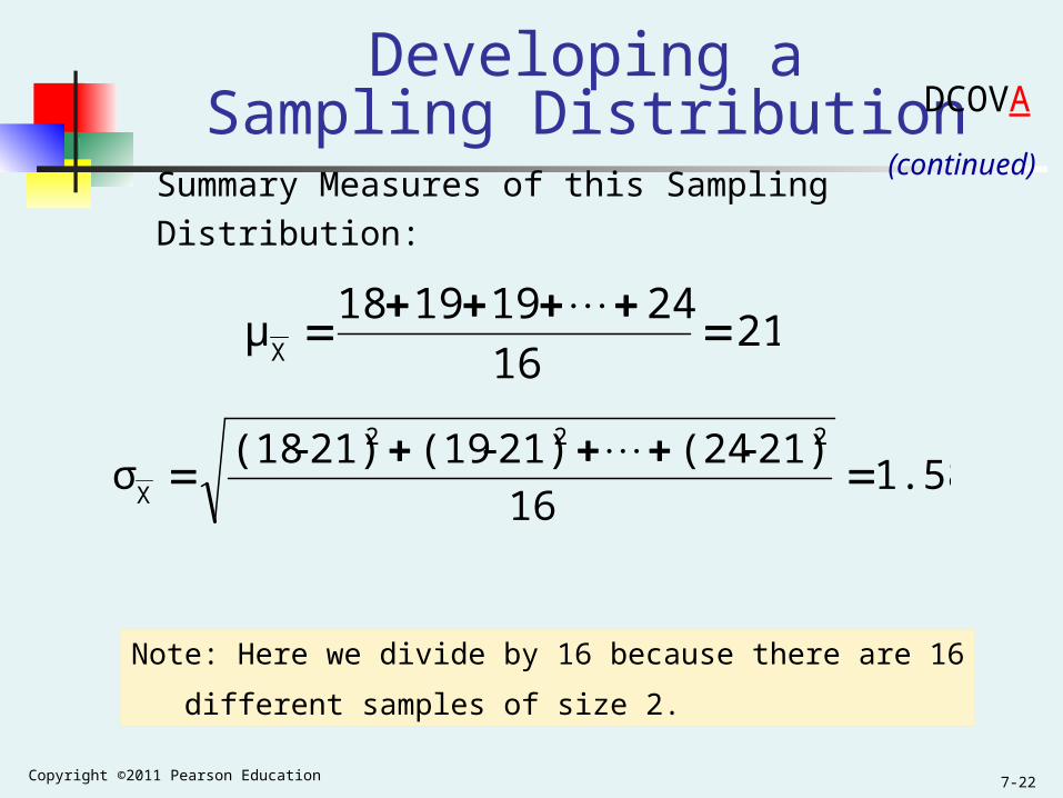
Summary Measures of this Sampling Distribution:

Developing aSampling Distribution

(continued)

2116

24191918μ

X

1.5816

21)-(2421)-(1921)-(18σ

222

X

DCOVA

Note: Here we divide by 16 because there are 16

different samples of size 2.


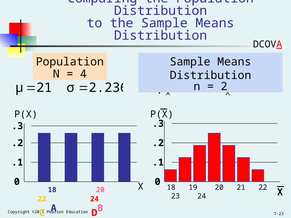
Comparing the Population Distributionto the Sample Means Distribution

18 19 20 21 22 23 240

.1

.2

.3 P(X)

X 18 20 22 24

A B C D

0

.1

.2

.3

PopulationN = 4

P(X)

X _

1.58σ 21μXX

2.236σ 21μ

Sample Means Distributionn = 2

_

DCOVA


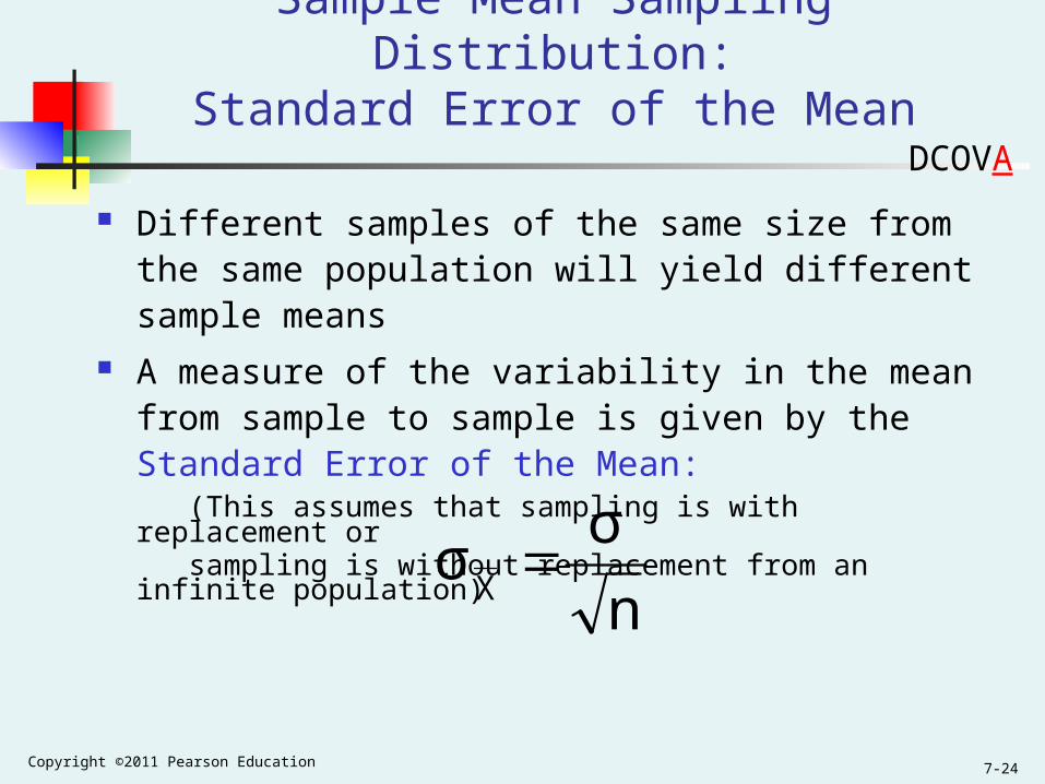
Sample Mean Sampling Distribution:Standard Error of the Mean

Different samples of the same size from the same population will yield different sample means

A measure of the variability in the mean from sample to sample is given by the Standard Error of the Mean:

(This assumes that sampling is with replacement or sampling is without replacement from an infinite

population)

Note that the standard error of the mean decreases as the sample size increases

n

σσ

X

DCOVA


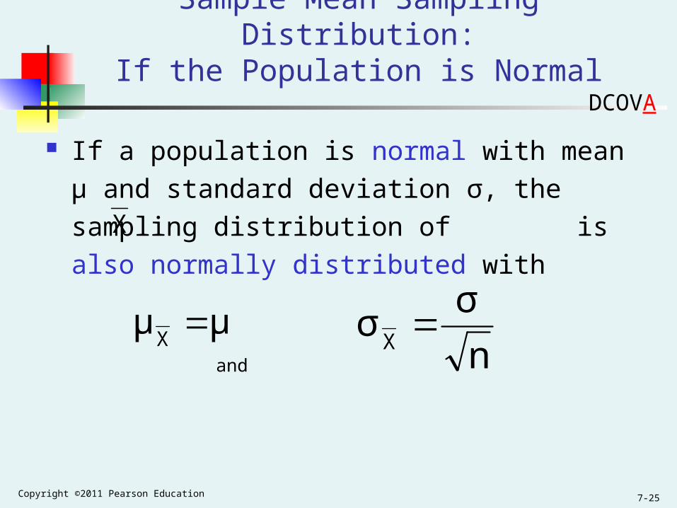
Sample Mean Sampling Distribution:If the Population is Normal

If a population is normal with mean μ and

standard deviation σ, the sampling distribution

of is also normally distributed with

and

X

μμX

n

σσ

X

DCOVA


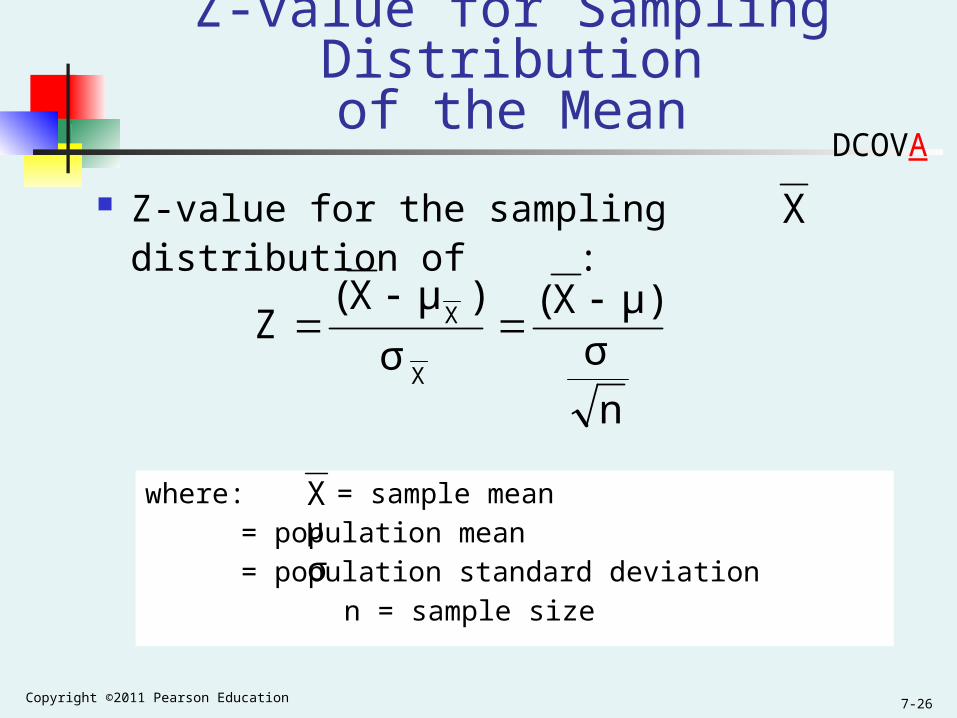
Z-value for Sampling Distributionof the Mean

Z-value for the sampling distribution of :

where: = sample mean

= population mean

= population standard deviation

n = sample size

Xμσ

n

σμ)X(

σ

)μX(Z

X

X

X

DCOVA


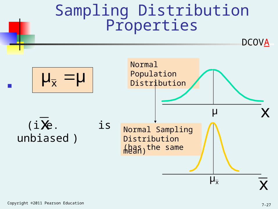
Normal Population Distribution

Normal Sampling Distribution (has the same mean)

Sampling Distribution Properties

(i.e. is unbiased )xx

x

μμx

μ

xμ

DCOVA


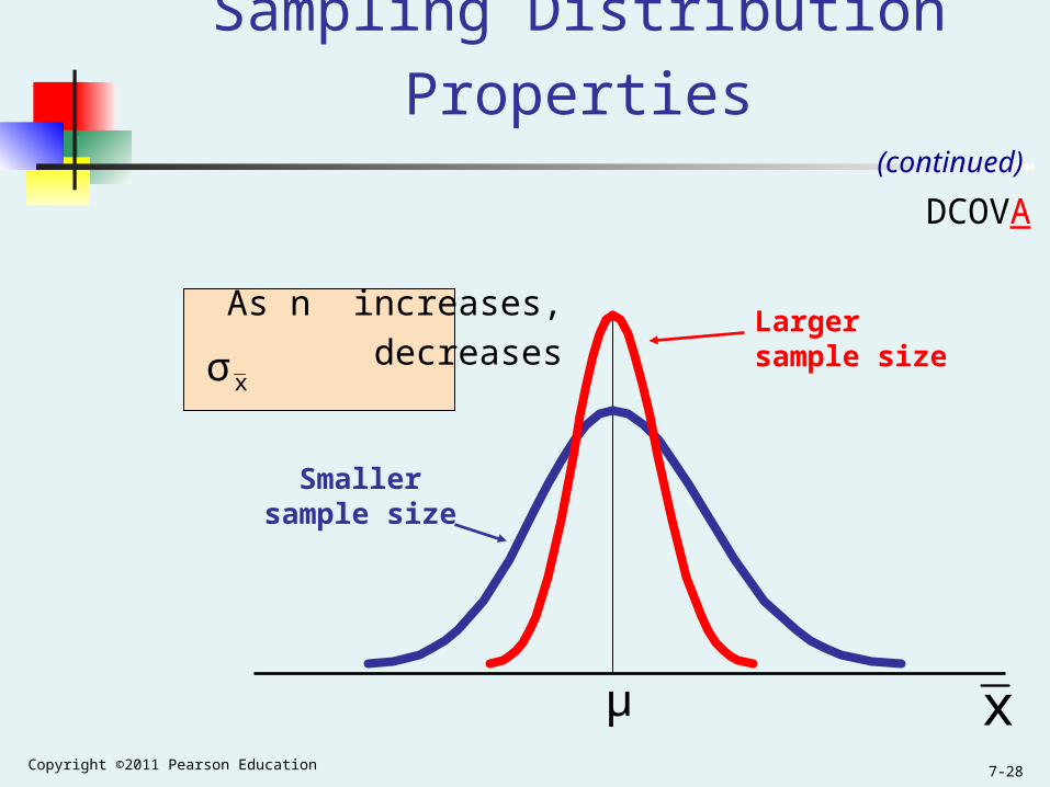
Sampling Distribution Properties

As n increases,

decreasesLarger sample size

Smaller sample size

x

(continued)

xσ

μ

DCOVA


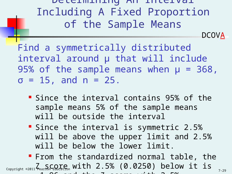
Determining An Interval Including A Fixed Proportion of the Sample Means

Find a symmetrically distributed interval around µ that will include 95% of the sample means when µ = 368, σ = 15, and n = 25.

Since the interval contains 95% of the sample means 5% of the sample means will be outside the interval

Since the interval is symmetric 2.5% will be above the upper limit and 2.5% will be below the lower limit.

From the standardized normal table, the Z score with 2.5% (0.0250) below it is -1.96 and the Z score with 2.5% (0.0250) above it is 1.96.

DCOVA


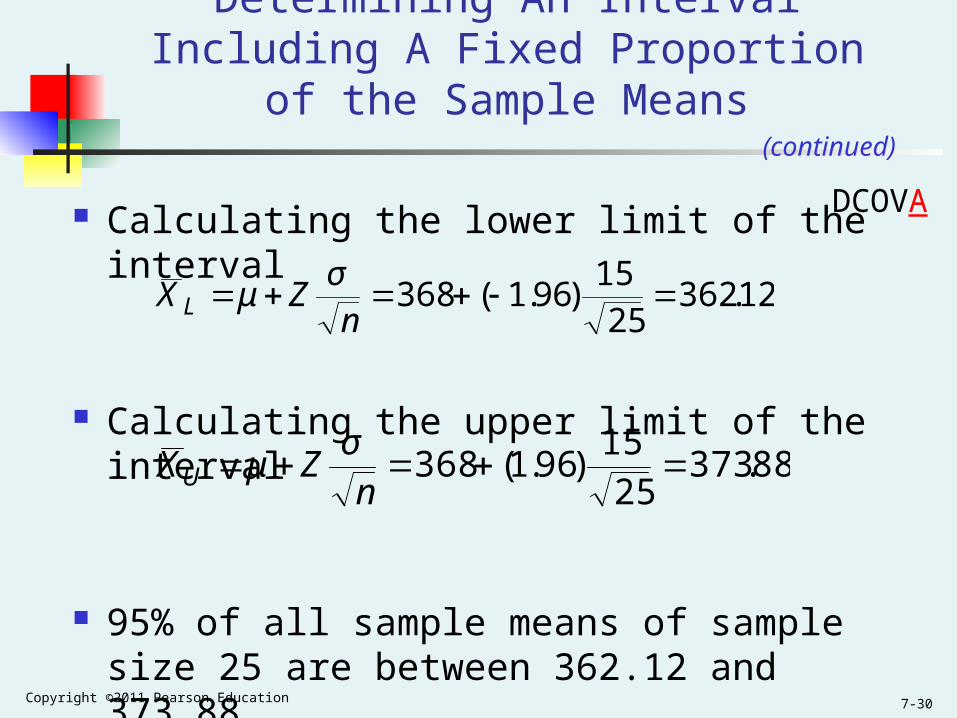
Determining An Interval Including A Fixed Proportion of the Sample Means

Calculating the lower limit of the interval

Calculating the upper limit of the interval

95% of all sample means of sample size 25 are between 362.12 and 373.88

12.36225

15)96.1(368

nZX L

σμ

(continued)

88.37325

15)96.1(368

nZXU

σμ

DCOVA


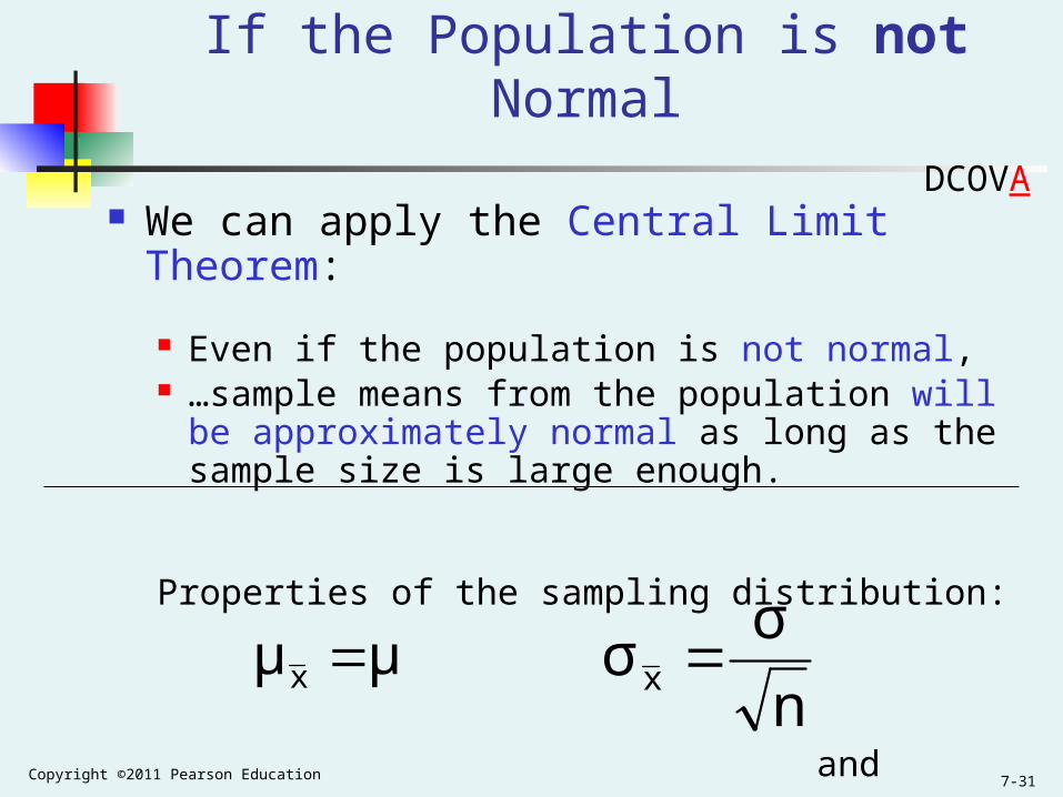
Sample Mean Sampling Distribution:If the Population is not Normal

We can apply the Central Limit Theorem:

Even if the population is not normal, …sample means from the population will be

approximately normal as long as the sample size is large enough.

Properties of the sampling distribution:

andμμx n

σσx

DCOVA


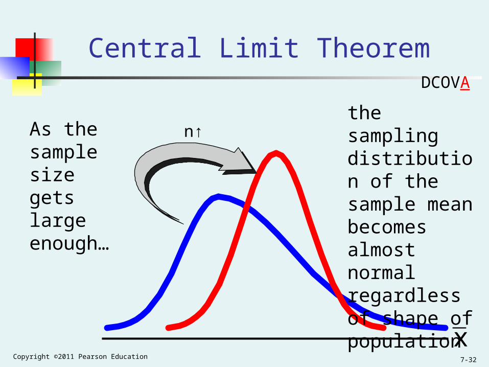
n↑

Central Limit Theorem

As the sample size gets large enough…

the sampling distribution of the sample mean becomes almost normal regardless of shape of population

x

DCOVA


Population Distribution

Sampling Distribution (becomes normal as n increases)

Central Tendency

Variation

x

x

Larger sample size

Smaller sample size

Sample Mean Sampling Distribution:If the Population is not Normal

(continued)

Sampling distribution properties:

μμx

n

σσx

xμ

μ

DCOVA


How Large is Large Enough?

For most distributions, n > 30 will give a sampling distribution that is nearly normal

For fairly symmetric distributions, n > 15

For normal population distributions, the sampling distribution of the mean is always normally distributed

DCOVA


Example

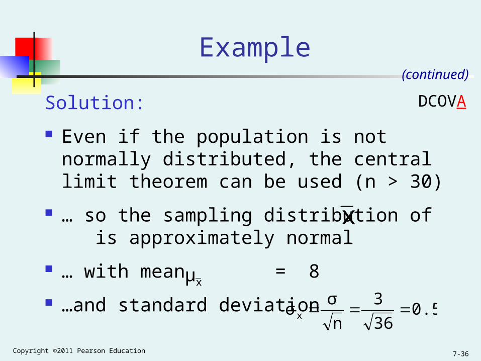
Suppose a population has mean μ = 8 and standard deviation σ = 3. Suppose a random sample of size n = 36 is selected.

What is the probability that the sample mean is between 7.8 and 8.2?

DCOVA


Example

Solution:

Even if the population is not normally distributed, the central limit theorem can be used (n > 30)

… so the sampling distribution of is approximately normal

… with mean = 8

…and standard deviation

(continued)

x

xμ

0.536

3

n

σσx

DCOVA


Example

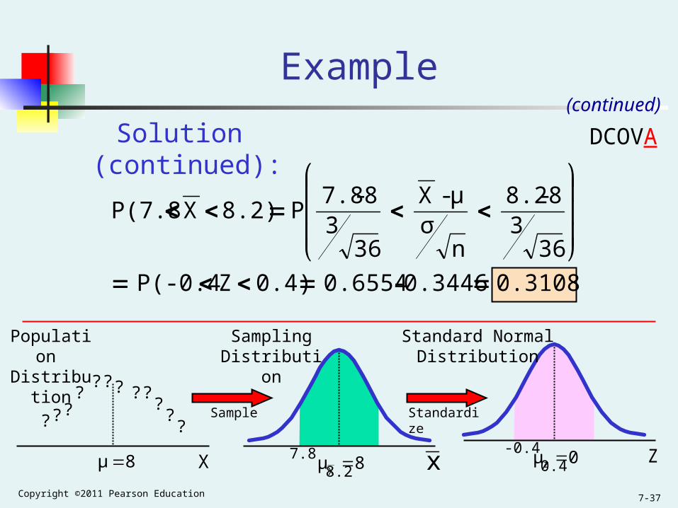
Solution (continued):(continued)

0.3108 0.3446 - 0.65540.4)ZP(-0.4

363

8-8.2

nσ

μ- X

363

8-7.8P 8.2) X P(7.8

Z7.8 8.2 -0.4 0.4

Sampling Distribution

Standard Normal Distribution

Population Distribution

??

??

?????

??? Sample Standardize

8μ 8μX

0μz xX

DCOVA


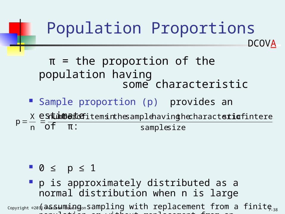
Population Proportions

π = the proportion of the population having some characteristic Sample proportion (p) provides an estimate of π:

0 ≤ p ≤ 1 p is approximately distributed as a normal distribution

when n is large(assuming sampling with replacement from a finite population or without replacement from an infinite population)

size sample

interest ofstic characteri the having sample the in itemsofnumber

n

Xp

DCOVA


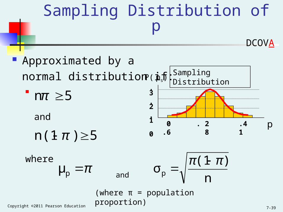
Sampling Distribution of p

Approximated by a

normal distribution if:

where

and

(where π = population proportion)

Sampling DistributionP( ps)

.3

.2

.1 0

0 . 2 .4 .6 8 1 p

πpμn

)(1σp

ππ

5)n(1

5n

and

π

π

DCOVA


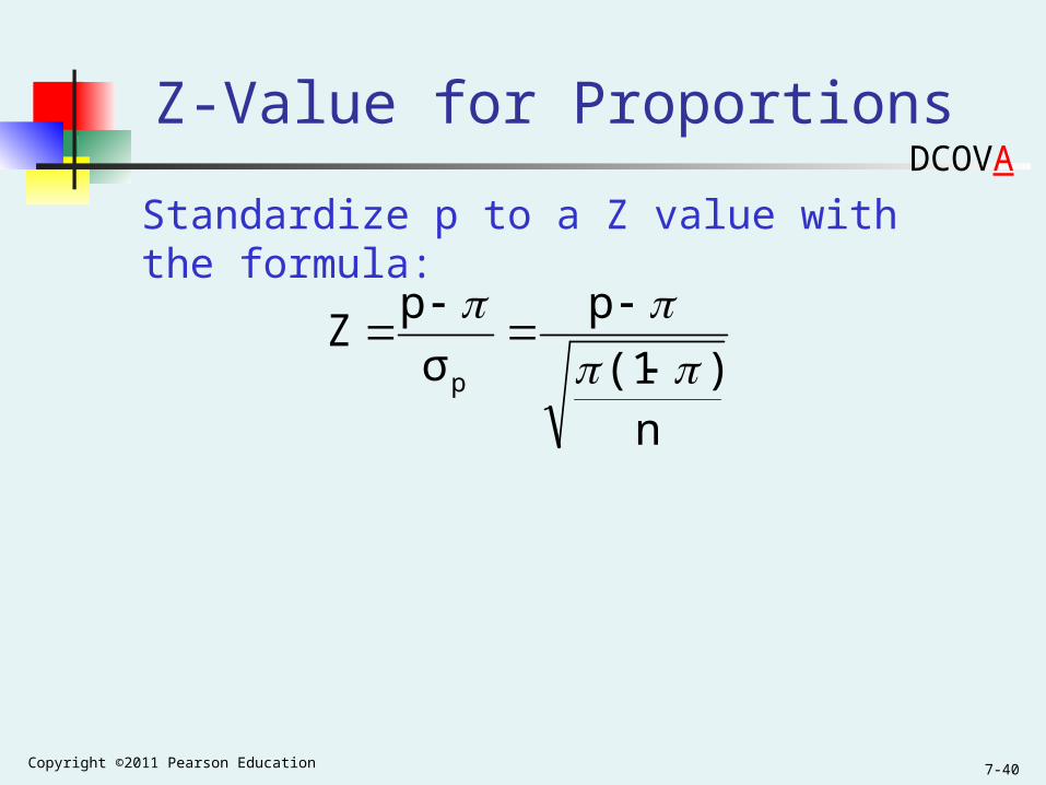
Z-Value for Proportions

n)(1

p

σ

pZ

p

Standardize p to a Z value with the formula:

DCOVA


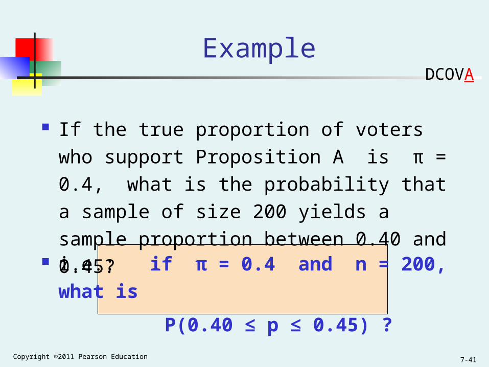
Example

If the true proportion of voters who support

Proposition A is π = 0.4, what is the probability

that a sample of size 200 yields a sample

proportion between 0.40 and 0.45?

i.e.: if π = 0.4 and n = 200, what is

P(0.40 ≤ p ≤ 0.45) ?

DCOVA


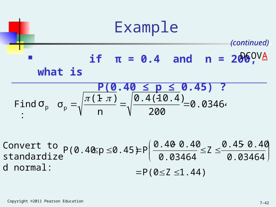
Example

if π = 0.4 and n = 200, what is

P(0.40 ≤ p ≤ 0.45) ?

(continued)

0.03464200

0.4)0.4(1

n

)(1σp

1.44)ZP(0

0.03464

0.400.45Z

0.03464

0.400.40P0.45)pP(0.40

Find :

Convert to standardized normal:

pσ

DCOVA


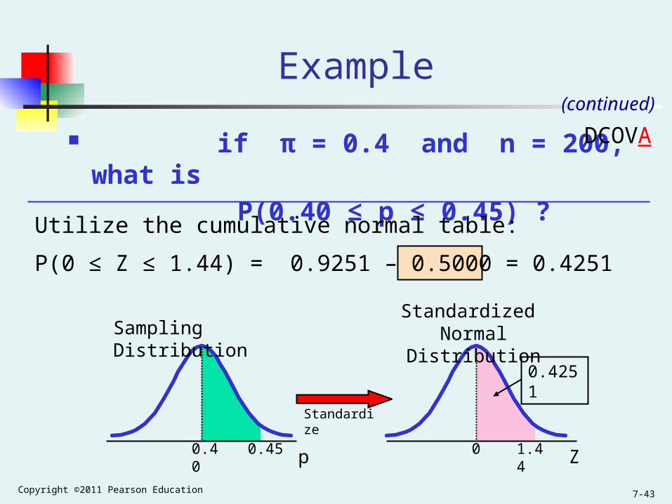
Example

Z0.45 1.44

0.4251

Standardize

Sampling DistributionStandardized

Normal Distribution

if π = 0.4 and n = 200, what is

P(0.40 ≤ p ≤ 0.45) ?

(continued)

Utilize the cumulative normal table:

P(0 ≤ Z ≤ 1.44) = 0.9251 – 0.5000 = 0.4251

0.40 0p

DCOVA


Chapter Summary

Discussed probability and nonprobability samples Described four common probability samples Examined survey worthiness and types of survey

errors Introduced sampling distributions Described the sampling distribution of the mean

For normal populations Using the Central Limit Theorem

Described the sampling distribution of a proportion Calculated probabilities using sampling distributions


Online Topic

Sampling From Finite Populations

Statistics for Managers using Microsoft Excel

6th Edition


Learning Objectives

In this chapter, you learn: To know when finite population corrections are

needed To know how to utilize finite population

corrections factors in calculating standard errors


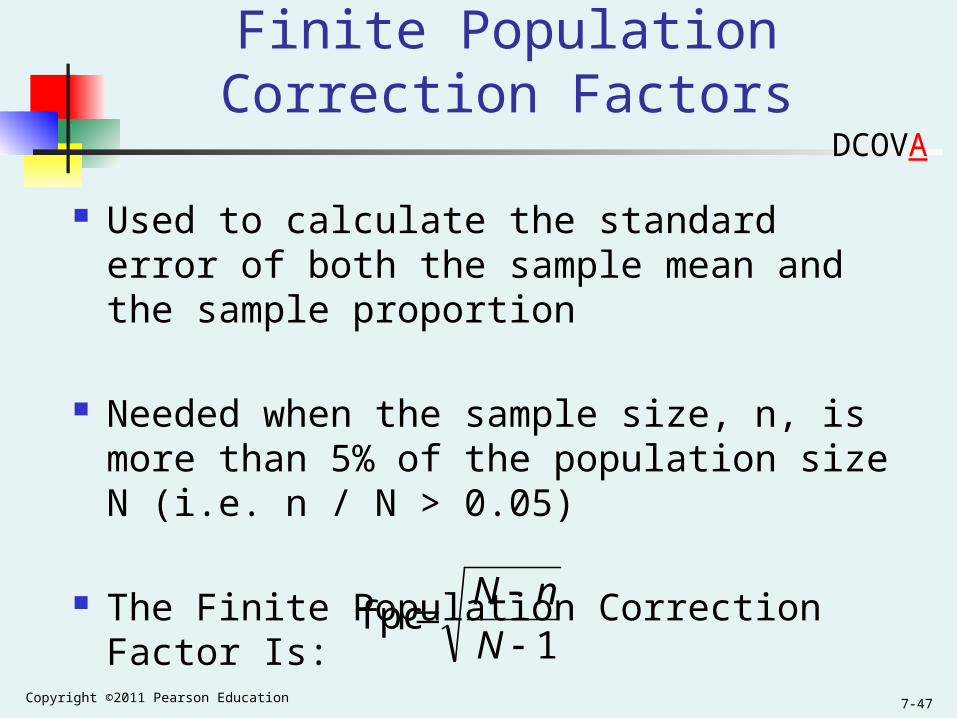
Finite Population Correction Factors

Used to calculate the standard error of both the sample mean and the sample proportion

Needed when the sample size, n, is more than 5% of the population size N (i.e. n / N > 0.05)

The Finite Population Correction Factor Is:

DCOVA

1 fpc

N

nN


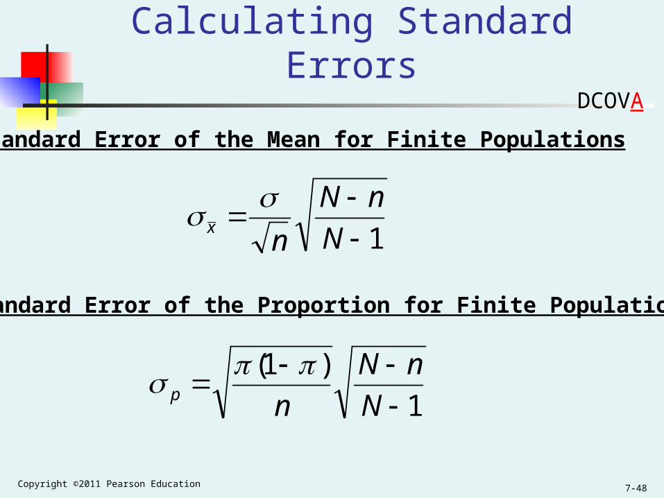
Using The fpc In Calculating Standard Errors

DCOVA

Standard Error of the Mean for Finite Populations

1

N

nN

nx

Standard Error of the Proportion for Finite Populations

1

)1(

N

nN

np


Using The fpc Reduces The Standard Error

The fpc is always less than 1

So when it is used it reduces the standard error

Resulting in more precise estimates of population parameters

DCOVA


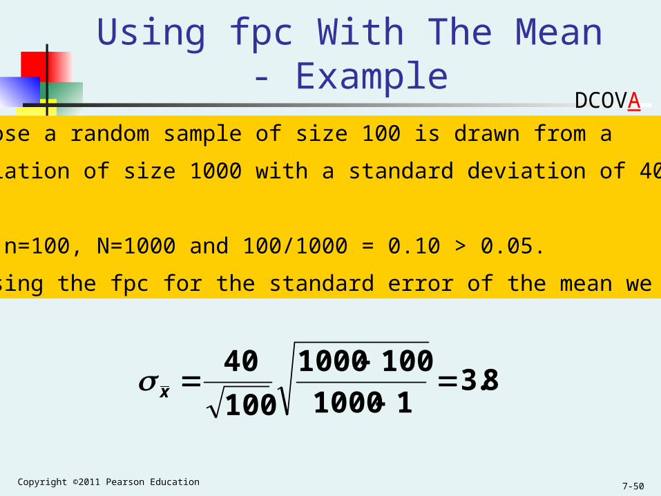
Using fpc With The Mean - Example

DCOVA

Suppose a random sample of size 100 is drawn from a

population of size 1000 with a standard deviation of 40.

Here n=100, N=1000 and 100/1000 = 0.10 > 0.05.

So using the fpc for the standard error of the mean we get:

8.311000

1001000

100

40

x


Section Summary

Identified when a finite population correction should be used.

Identified how to utilize a finite population correction factor in calculating the standard error of both a sample mean and a sample proportion


All rights reserved. No part of this publication may be reproduced, stored in a retrieval system, or transmitted, in any form or by any means, electronic, mechanical, photocopying,

recording, or otherwise, without the prior written permission of the publisher. Printed in the United States of America.

Documents

Copyright ©2011 Pearson Education 7-1 Chapter 7 Sampling and Sampling Distributions Statistics for Managers using Microsoft Excel 6 th Global Edition