Copyright © 2011 Pearson Addison-Wesley. All rights reserved. Nonlinear Regression Functions Chapter 8

Copyright © 2011 Pearson Addison-Wesley. All rights reserved.

Nonlinear Regression Functions

Chapter 8


Outline

1. Nonlinear regression functions – general comments

2. Nonlinear functions of one variable3. Nonlinear functions of two variables:

interactions4. Application to the California Test Score

data set

8-2


Nonlinear regression functions

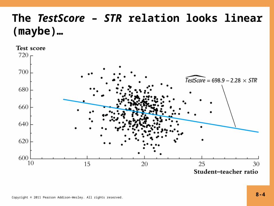
• The regression functions so far have been linear in the X’s

• But the linear approximation is not always a good one

• The multiple regression model can handle regression functions that are nonlinear in one or more X.

8-3


The TestScore – STR relation looks linear (maybe)…

8-4


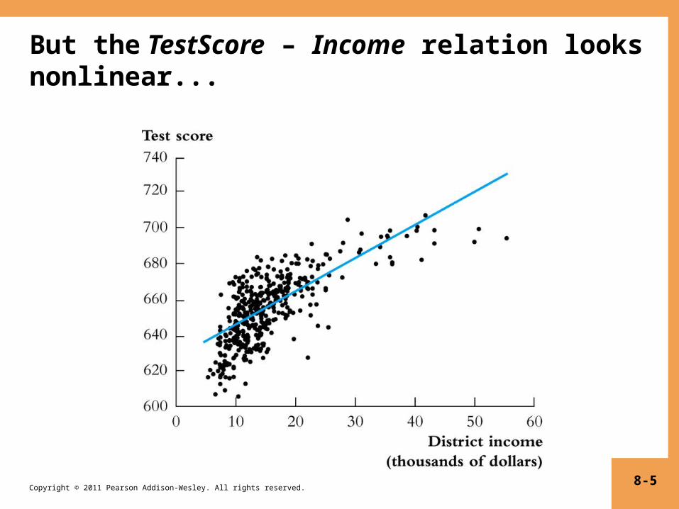
But the TestScore – Income relation looks nonlinear...

8-5


Nonlinear Regression Population Regression Functions – General Ideas(SW Section 8.1)

If a relation between Y and X is nonlinear:• The effect on Y of a change in X depends on the value of X –

that is, the marginal effect of X is not constant• A linear regression is mis-specified: the functional form is

wrong• The estimator of the effect on Y of X is biased: in general it

isn’t even right on average.• The solution is to estimate a regression function that is

nonlinear in X

8-6


The general nonlinear population regression function

Yi = f(X1i, X2i,…, Xki) + ui, i = 1,…, n

Assumptions1. E(ui| X1i, X2i,…, Xki) = 0 (same); implies that f is the

conditional expectation of Y given the X’s.2. (X1i,…, Xki, Yi) are i.i.d. (same).

3. Big outliers are rare (same idea; the precise mathematical condition depends on the specific f).

4. No perfect multicollinearity (same idea; the precise statement depends on the specific f).

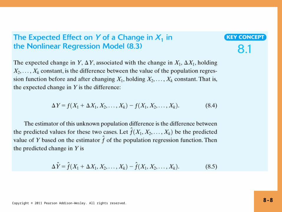
The change in Y associated with a change in X1, holding X2,…,

Xk constant is:

ΔY = f(X1 + ΔX1, X2,…, Xk) – f(X1, X2,…, Xk) 8-7

Copyright © 2011 Pearson Addison-Wesley. All rights reserved. 8-8


Nonlinear Functions of a Single Independent Variable (SW Section 8.2)

We’ll look at two complementary approaches: 1. Polynomials in X

The population regression function is approximated by a quadratic, cubic, or higher-degree polynomial

2. Logarithmic transformations

Y and/or X is transformed by taking its logarithmthis gives a “percentages” interpretation that makes sense in many applications

8-9


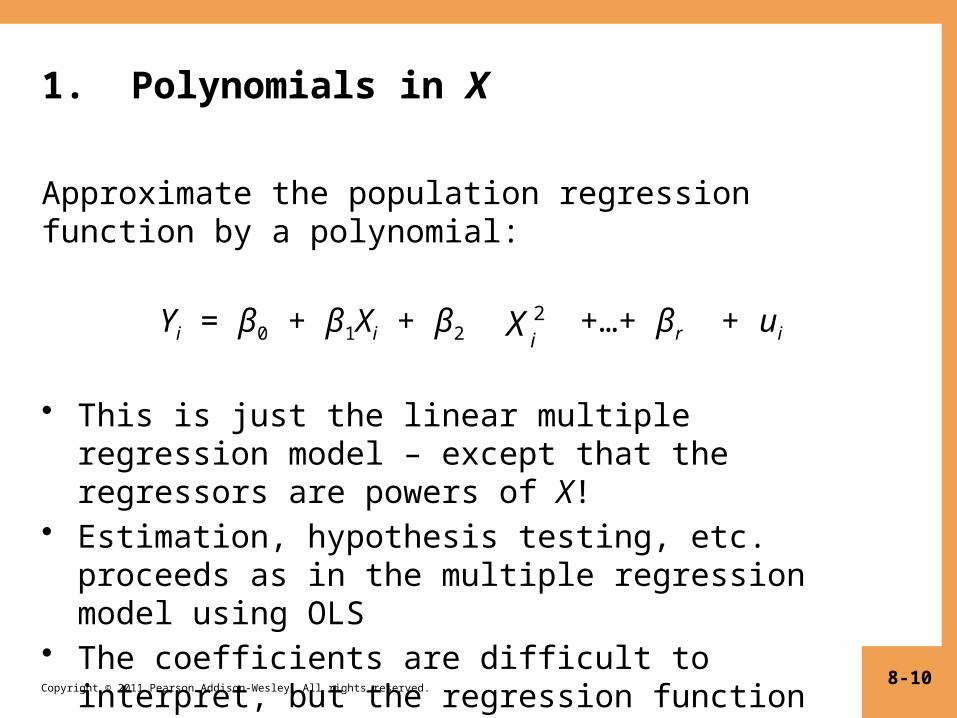
1. Polynomials in X

Approximate the population regression function by a polynomial:

Yi = β0 + β1Xi + β2 +…+ βr + ui

• This is just the linear multiple regression model –

except that the regressors are powers of X!• Estimation, hypothesis testing, etc. proceeds as in

the multiple regression model using OLS• The coefficients are difficult to interpret, but the

regression function itself is interpretable

8-10

X i2


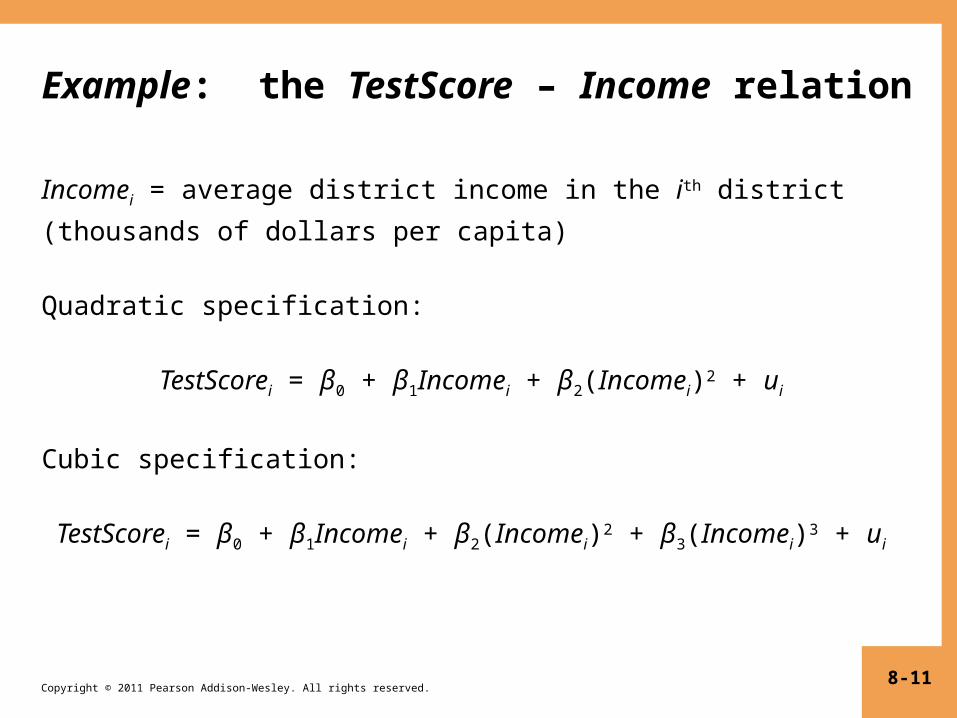
Example: the TestScore – Income relation

Incomei = average district income in the ith district

(thousands of dollars per capita) Quadratic specification:

TestScorei = β0 + β1Incomei + β2(Incomei)2 + ui

Cubic specification: TestScorei = β0 + β1Incomei + β2(Incomei)2 + β3(Incomei)3 + ui

8-11


Estimation of the quadratic specification in STATA generate avginc2 = avginc*avginc; Create a new regressor reg testscr avginc avginc2, r; Regression with robust standard errors Number of obs = 420 F( 2, 417) = 428.52 Prob > F = 0.0000 R-squared = 0.5562 Root MSE = 12.724 ------------------------------------------------------------------------------ | Robust testscr | Coef. Std. Err. t P>|t| [95% Conf. Interval]-------------+---------------------------------------------------------------- avginc | 3.850995 .2680941 14.36 0.000 3.32401 4.377979 avginc2 | -.0423085 .0047803 -8.85 0.000 -.051705 -.0329119 _cons | 607.3017 2.901754 209.29 0.000 601.5978 613.0056------------------------------------------------------------------------------

Test the null hypothesis of linearity against the alternative that the regression function is a quadratic….

8-12


Interpreting the estimated regression function:

(a) Plot the predicted values

= 607.3 + 3.85Incomei – 0.0423(Incomei)2

(2.9) (0.27) (0.0048)

8-13

TestScore


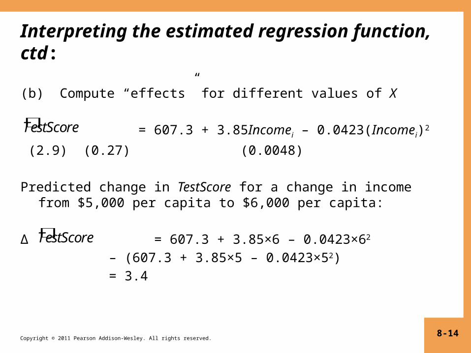
Interpreting the estimated regression function, ctd:

(b) Compute “effects” for different values of X = 607.3 + 3.85Incomei – 0.0423(Incomei)2

(2.9) (0.27) (0.0048) Predicted change in TestScore for a change in income from

$5,000 per capita to $6,000 per capita: Δ = 607.3 + 3.85×6 – 0.0423×62

– (607.3 + 3.85×5 – 0.0423×52)= 3.4

8-14

TestScore

TestScore


= 607.3 + 3.85Incomei – 0.0423(Incomei)2

Predicted “effects” for different values of X:

The “effect” of a change in income is greater at low than high income levels (perhaps, a declining marginal benefit of an increase in school budgets?)Caution! What is the effect of a change from 65 to 66? Don’t extrapolate outside the range of the data!

8-15

Change in Income ($1000 per capita) Δ

from 5 to 6 3.4

from 25 to 26 1.7

from 45 to 46 0.0

TestScore

TestScore


Estimation of a cubic specification in STATA

gen avginc3 = avginc*avginc2; Create the cubic regressorreg testscr avginc avginc2 avginc3, r; Regression with robust standard errors Number of obs = 420 F( 3, 416) = 270.18 Prob > F = 0.0000 R-squared = 0.5584 Root MSE = 12.707 ------------------------------------------------------------------------------ | Robust testscr | Coef. Std. Err. t P>|t| [95% Conf. Interval]-------------+---------------------------------------------------------------- avginc | 5.018677 .7073505 7.10 0.000 3.628251 6.409104 avginc2 | -.0958052 .0289537 -3.31 0.001 -.1527191 -.0388913 avginc3 | .0006855 .0003471 1.98 0.049 3.27e-06 .0013677 _cons | 600.079 5.102062 117.61 0.000 590.0499 610.108------------------------------------------------------------------------------

8-16


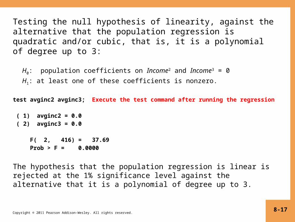
Testing the null hypothesis of linearity, against the alternative that the population regression is quadratic and/or cubic, that is, it is a polynomial of degree up to 3:

H0: population coefficients on Income2 and Income3 = 0

H1: at least one of these coefficients is nonzero.

test avginc2 avginc3; Execute the test command after running the regression ( 1) avginc2 = 0.0 ( 2) avginc3 = 0.0 F( 2, 416) = 37.69 Prob > F = 0.0000

The hypothesis that the population regression is linear is rejected at the 1% significance level against the alternative that it is a polynomial of degree up to 3.

8-17


Summary: polynomial regression functions

Yi = β0 + β1Xi + β2 +…+ βr + ui

• Estimation: by OLS after defining new regressors• Coefficients have complicated interpretations• To interpret the estimated regression function:

– plot predicted values as a function of x– compute predicted ΔY/ΔX at different values of x

• Hypotheses concerning degree r can be tested by t- and F-tests on the appropriate (blocks of) variable(s).

• Choice of degree r– plot the data; t- and F-tests, check sensitivity of estimated

effects; judgment.– Or use model selection criteria (later)

8-18


2. Logarithmic functions of Y and/or X

• ln(X) = the natural logarithm of X• Logarithmic transforms permit modeling relations in

“percentage” terms (like elasticities), rather than linearly.

Here’s why: ln(x+Δx) – ln(x) = ≅

(calculus: )Numerically: ln(1.01) = .00995 ≅ .01; ln(1.10) = .0953 ≅ .10 (sort of)

8-19

ln 1

x

x

x

x

d ln(x)

dx

1

x


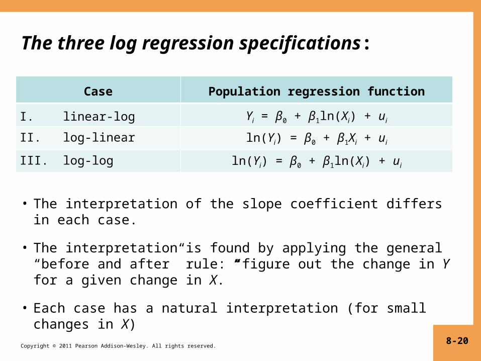
The three log regression specifications:

Case Population regression function

I. linear-log Yi = β0 + β1ln(Xi) + ui

II. log-linear ln(Yi) = β0 + β1Xi + ui

III. log-log ln(Yi) = β0 + β1ln(Xi) + ui

8-20

• The interpretation of the slope coefficient differs in each case.

• The interpretation is found by applying the general “before and after” rule: “figure out the change in Y for a given change in X.”

• Each case has a natural interpretation (for small changes in X)


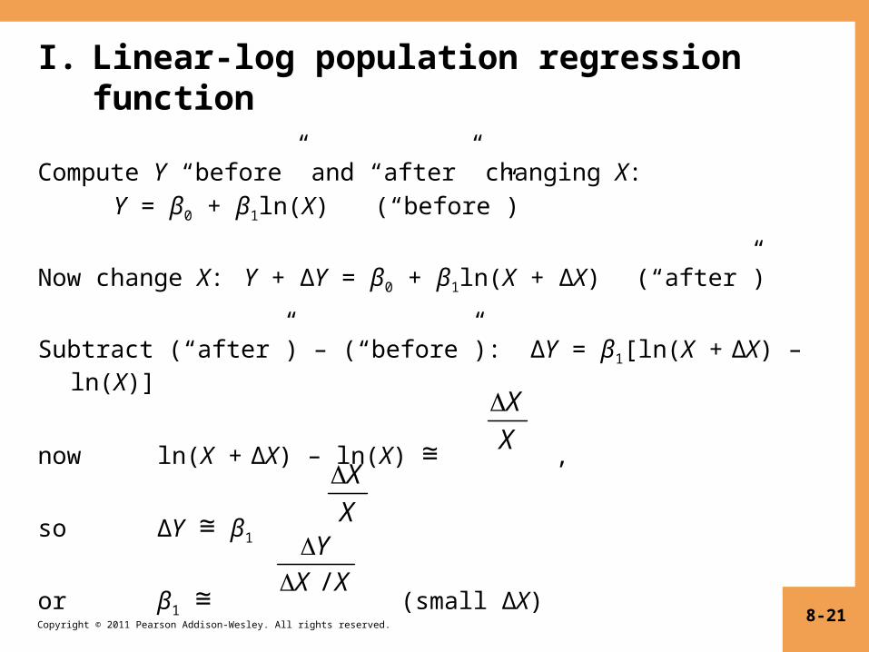
I. Linear-log population regression function

Compute Y “before” and “after” changing X:Y = β0 + β1ln(X) (“before”)

Now change X: Y + ΔY = β0 + β1ln(X + ΔX) (“after”)

Subtract (“after”) – (“before”): ΔY = β1[ln(X + ΔX) – ln(X)]

now ln(X + ΔX) – ln(X) ≅ ,

so ΔY ≅ β1

or β1 ≅ (small ΔX)

8-21

X

X

X

X

Y

X / X


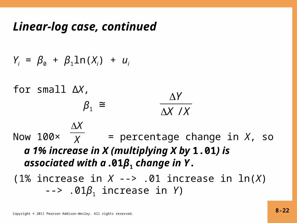
Linear-log case, continued

Yi = β0 + β1ln(Xi) + ui

for small ΔX,

β1 ≅

Now 100× = percentage change in X, so a 1% increase in X (multiplying X by 1.01) is associated with a .01β1 change in Y.

(1% increase in X --> .01 increase in ln(X) --> .01β1 increase in Y)

8-22

Y

X / X

X

X


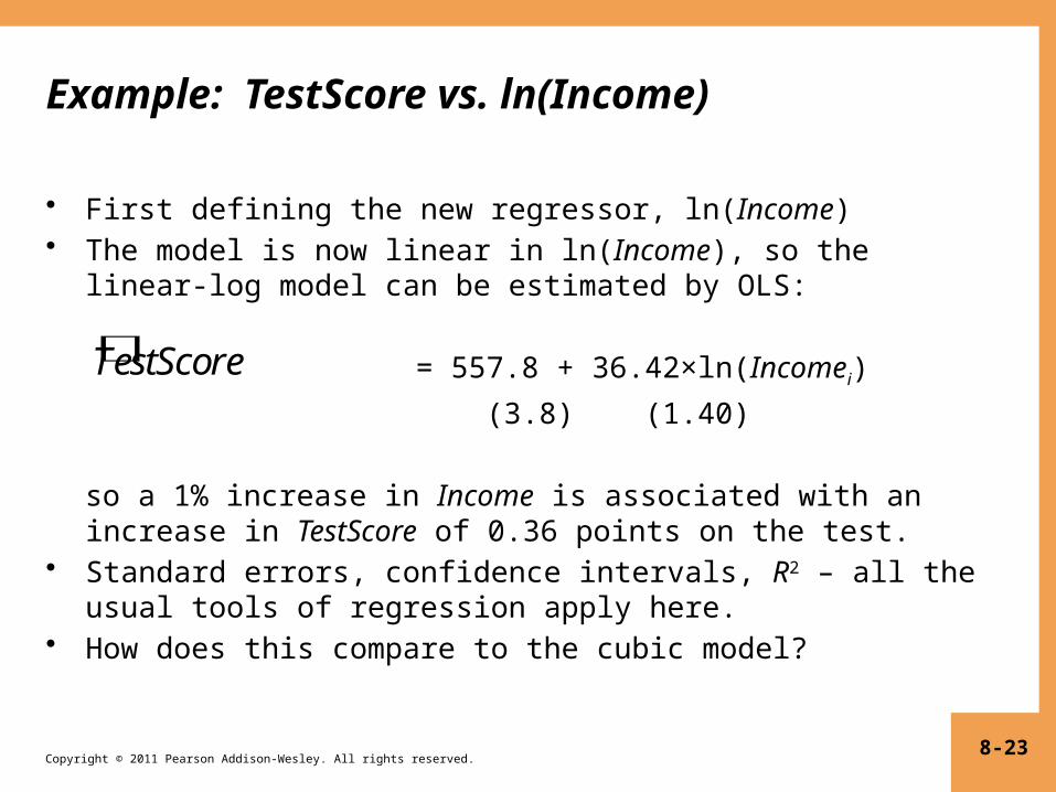
Example: TestScore vs. ln(Income)

• First defining the new regressor, ln(Income)• The model is now linear in ln(Income), so the linear-log

model can be estimated by OLS: = 557.8 + 36.42×ln(Incomei)

(3.8) (1.40)

so a 1% increase in Income is associated with an increase in TestScore of 0.36 points on the test.

• Standard errors, confidence intervals, R2 – all the usual tools of regression apply here.

• How does this compare to the cubic model?

8-23

TestScore


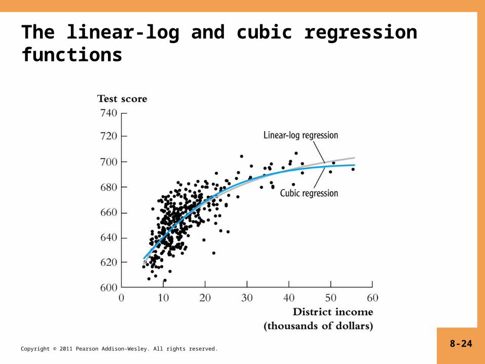
The linear-log and cubic regression functions

8-24


II. Log-linear population regression function

ln(Y) = β0 + β1X (b)

Now change X: ln(Y + ΔY) = β0 + β1(X + ΔX) (a)

Subtract (a) – (b): ln(Y + ΔY) – ln(Y) = β1ΔX

so ≅ β1ΔX


8-25

Y

Y

Y / Y

X


Log-linear case, continued

ln(Yi) = β0 + β1Xi + ui

for small ΔX, β1 ≅

• Now 100× = percentage change in Y, so a change in X by one unit (ΔX = 1) is associated with a 100β1%

change in Y.

• 1 unit increase in X β1 increase in ln(Y)

100β1% increase in Y

• Note: What are the units of ui and the SER? o fractional (proportional) deviationso for example, SER = .2 means…

8-26

Y / Y

X

Y

Y


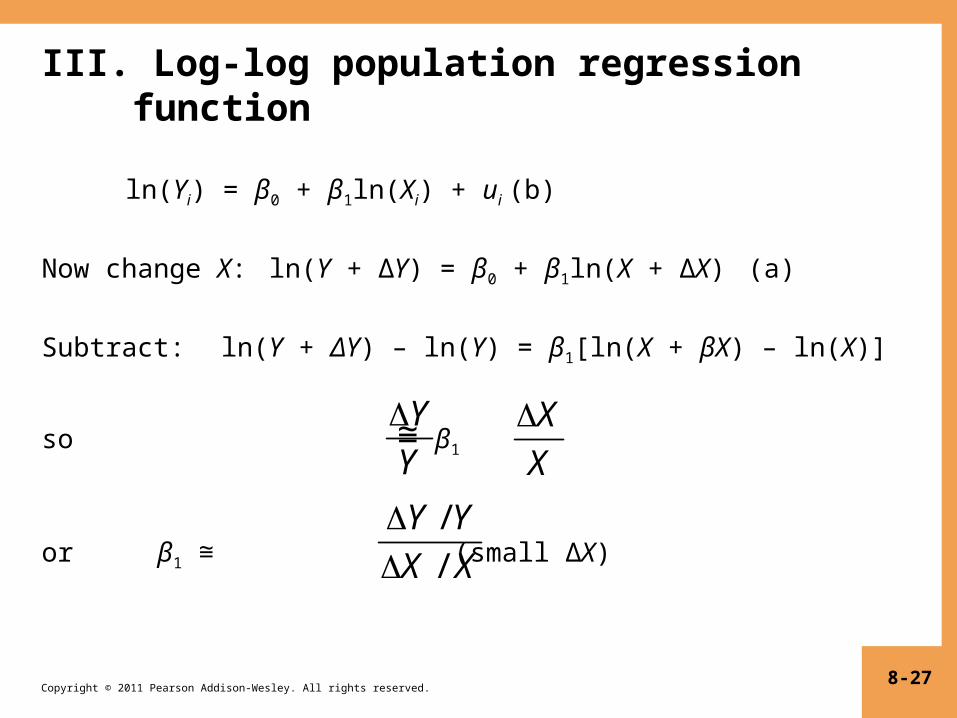
III. Log-log population regression function

ln(Yi) = β0 + β1ln(Xi) + ui (b)

Now change X: ln(Y + ΔY) = β0 + β1ln(X + ΔX) (a)

Subtract: ln(Y + ΔY) – ln(Y) = β1[ln(X + βX) – ln(X)]

so ≅ β1


8-27

Y

Y

X

X

Y / Y

X / X


Log-log case, continued

ln(Yi) = β0 + β1ln(Xi) + ui

for small ΔX,

β1 ≅

Now 100× = percentage change in Y, and 100× =

percentage change in X, so a 1% change in X is associated with a β1% change in Y.

In the log-log specification, β1 has the interpretation of

an elasticity.

8-28

Y

Y

Y / Y

X / X

X

X


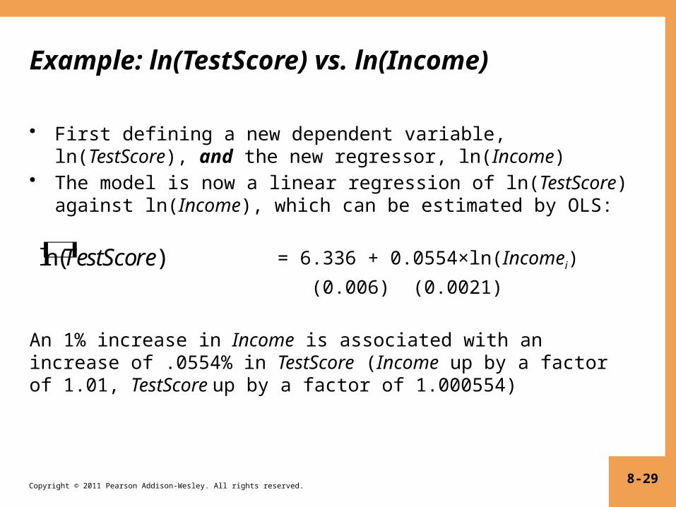
Example: ln(TestScore) vs. ln(Income)

• First defining a new dependent variable, ln(TestScore), and the new regressor, ln(Income)

• The model is now a linear regression of ln(TestScore) against ln(Income), which can be estimated by OLS:

= 6.336 + 0.0554×ln(Incomei)

(0.006) (0.0021) An 1% increase in Income is associated with an increase of .0554% in TestScore (Income up by a factor of 1.01, TestScore up by a factor of 1.000554)

8-29

ln( )TestScore


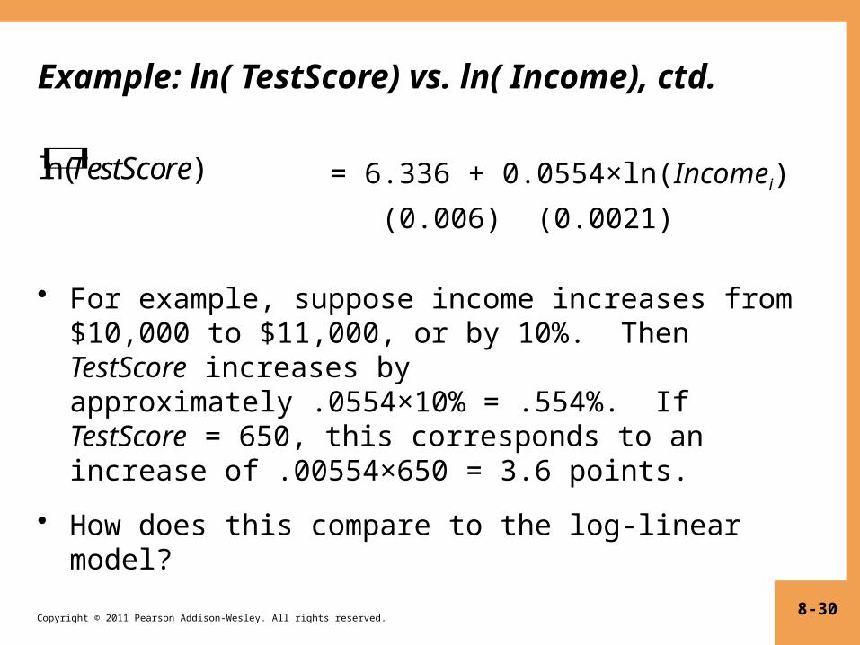
Example: ln( TestScore) vs. ln( Income), ctd.

= 6.336 + 0.0554×ln(Incomei)

(0.006) (0.0021) • For example, suppose income increases from

$10,000 to $11,000, or by 10%. Then TestScore increases by approximately .0554×10% = .554%. If TestScore = 650, this corresponds to an increase of .00554×650 = 3.6 points.

• How does this compare to the log-linear model?

8-30

ln( )TestScore


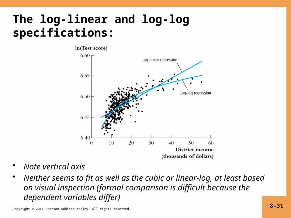
The log-linear and log-log specifications:

• Note vertical axis• Neither seems to fit as well as the cubic or linear-log, at least

based on visual inspection (formal comparison is difficult because the dependent variables differ)

8-31


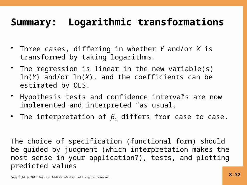
Summary: Logarithmic transformations

• Three cases, differing in whether Y and/or X is transformed by taking logarithms.

• The regression is linear in the new variable(s) ln(Y) and/or ln(X), and the coefficients can be estimated by OLS.

• Hypothesis tests and confidence intervals are now implemented and interpreted “as usual.”

• The interpretation of β1 differs from case to case.

The choice of specification (functional form) should be guided by judgment (which interpretation makes the most sense in your application?), tests, and plotting predicted values

8-32


Other nonlinear functions (and nonlinear least squares) (SW Appendix 8.1)

The foregoing regression functions have limitations…• Polynomial: test score can decrease with income• Linear-log: test score increases with income, but without

bound• Here is a nonlinear function in which Y always increases with

X and there is a maximum (asymptote) value of Y:

Y =

β0, β1, and α are unknown parameters. This is called a negative exponential growth curve. The asymptote as X → ∞ is β0.

8-33

0 e 1X


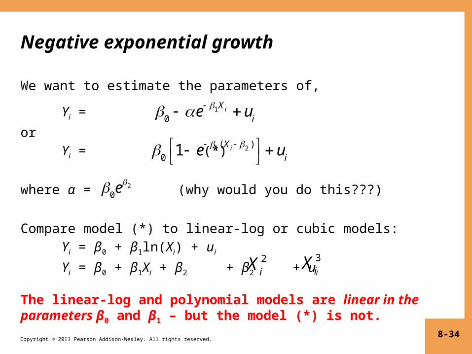
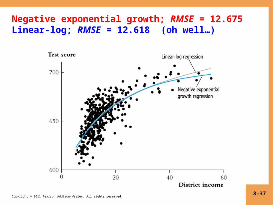
Negative exponential growth

We want to estimate the parameters of,

Yi =

orYi = (*)

where α = (why would you do this???)

Compare model (*) to linear-log or cubic models:

Yi = β0 + β1ln(Xi) + ui

Yi = β0 + β1Xi + β2 + β2 + ui

The linear-log and polynomial models are linear in the parameters β0 and β1 – but the model (*) is not.

8-34

0 e 1X i u

i

01 e 1 ( X i 2 )

u

i

0e2

X i2

X i3


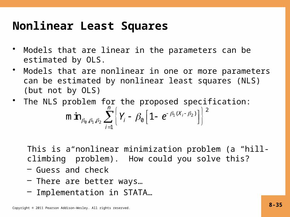
Nonlinear Least Squares

• Models that are linear in the parameters can be estimated by OLS.

• Models that are nonlinear in one or more parameters can be estimated by nonlinear least squares (NLS) (but not by OLS)

• The NLS problem for the proposed specification:

This is a nonlinear minimization problem (a “hill-climbing” problem). How could you solve this?– Guess and check– There are better ways…– Implementation in STATA…

8-35

1 2

0 1 2

2( )

, , 01

min 1 i

nX

ii

Y e


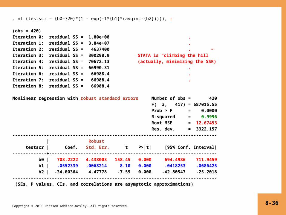
. nl (testscr = {b0=720}*(1 - exp(-1*{b1}*(avginc-{b2})))), r (obs = 420)Iteration 0: residual SS = 1.80e+08 .Iteration 1: residual SS = 3.84e+07 .Iteration 2: residual SS = 4637400 .Iteration 3: residual SS = 300290.9 STATA is “climbing the hill”Iteration 4: residual SS = 70672.13 (actually, minimizing the SSR)Iteration 5: residual SS = 66990.31 .Iteration 6: residual SS = 66988.4 .Iteration 7: residual SS = 66988.4 .Iteration 8: residual SS = 66988.4 Nonlinear regression with robust standard errors Number of obs = 420 F( 3, 417) = 687015.55 Prob > F = 0.0000 R-squared = 0.9996 Root MSE = 12.67453 Res. dev. = 3322.157------------------------------------------------------------------------------ | Robust testscr | Coef. Std. Err. t P>|t| [95% Conf. Interval]-------------+---------------------------------------------------------------- b0 | 703.2222 4.438003 158.45 0.000 694.4986 711.9459 b1 | .0552339 .0068214 8.10 0.000 .0418253 .0686425 b2 | -34.00364 4.47778 -7.59 0.000 -42.80547 -25.2018------------------------------------------------------------------------------ (SEs, P values, CIs, and correlations are asymptotic approximations)

8-36


Negative exponential growth; RMSE = 12.675Linear-log; RMSE = 12.618 (oh well…)

8-37


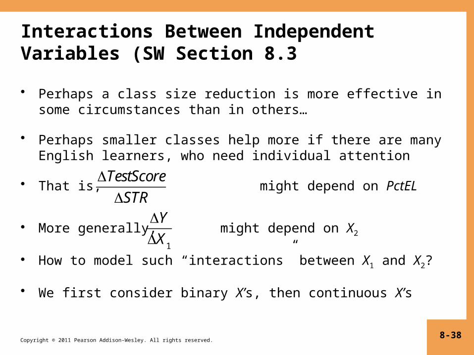
Interactions Between Independent Variables (SW Section 8.3

• Perhaps a class size reduction is more effective in some circumstances than in others…

• Perhaps smaller classes help more if there are many English learners, who need individual attention

• That is, might depend on PctEL

• More generally, might depend on X2

• How to model such “interactions” between X1 and X2?

• We first consider binary X’s, then continuous X’s

8-38

TestScore

STR

Y

X1


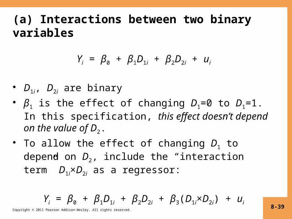
(a) Interactions between two binary variables

Yi = β0 + β1D1i + β2D2i + ui

• D1i, D2i are binary

• β1 is the effect of changing D1=0 to D1=1. In this specification, this effect doesn’t depend on the value of D2.

• To allow the effect of changing D1 to depend on D2, include the “interaction term” D1i×D2i as a regressor:

Yi = β0 + β1D1i + β2D2i + β3(D1i×D2i) + ui

8-39


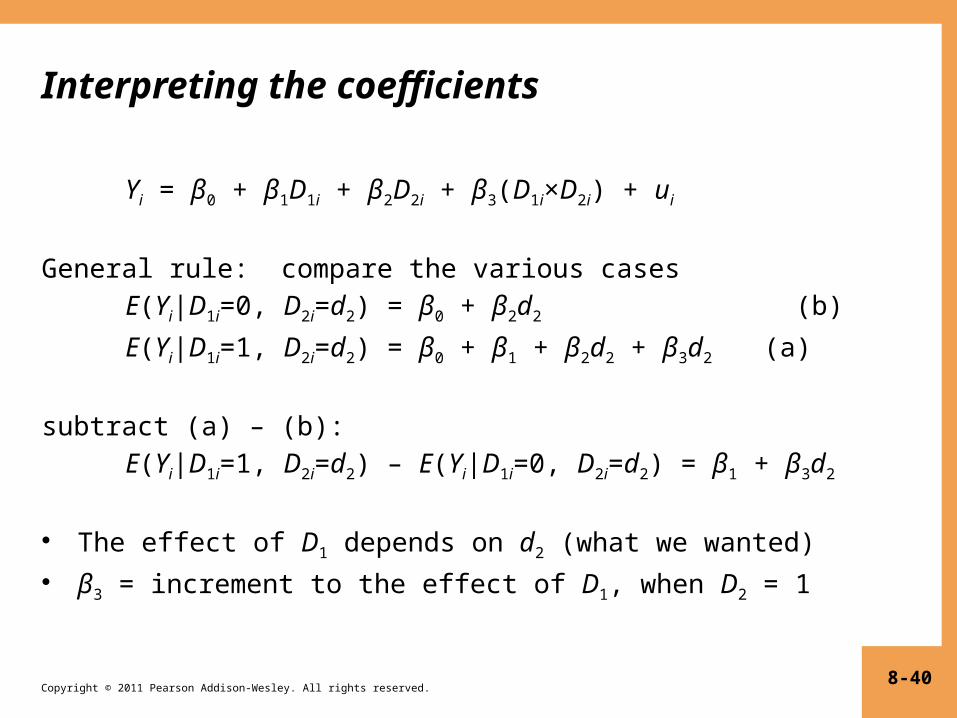
Interpreting the coefficients

Yi = β0 + β1D1i + β2D2i + β3(D1i×D2i) + ui

General rule: compare the various cases

E(Yi|D1i=0, D2i=d2) = β0 + β2d2

(b)E(Yi|D1i=1, D2i=d2) = β0 + β1 + β2d2 + β3d2 (a)

subtract (a) – (b):

E(Yi|D1i=1, D2i=d2) – E(Yi|D1i=0, D2i=d2) = β1 + β3d2

• The effect of D1 depends on d2 (what we wanted)

• β3 = increment to the effect of D1, when D2 = 1

8-40


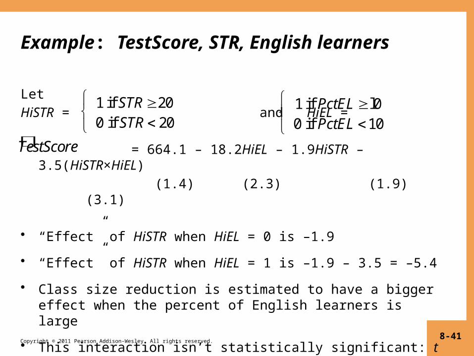
Example: TestScore, STR, English learners

LetHiSTR = and HiEL = = 664.1 – 18.2HiEL – 1.9HiSTR – 3.5(HiSTR×HiEL) (1.4) (2.3) (1.9) (3.1) • “Effect” of HiSTR when HiEL = 0 is –1.9

• “Effect” of HiSTR when HiEL = 1 is –1.9 – 3.5 = –5.4

• Class size reduction is estimated to have a bigger effect when the percent of English learners is large

• This interaction isn’t statistically significant: t = 3.5/3.1

8-41

1 if STR 200 if STR 20

1 if PctEL l00 if PctEL 10

TestScore


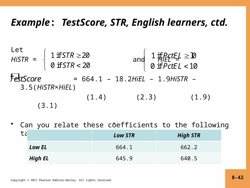
Example: TestScore, STR, English learners, ctd.

LetHiSTR = and HiEL = = 664.1 – 18.2HiEL – 1.9HiSTR – 3.5(HiSTR×HiEL) (1.4) (2.3) (1.9) (3.1) • Can you relate these coefficients to the following table of

group (“cell”) means?

8-42

1 if STR 200 if STR 20

1 if PctEL l00 if PctEL 10

TestScore

Low STR High STR

Low EL 664.1 662.2

High EL 645.9 640.5


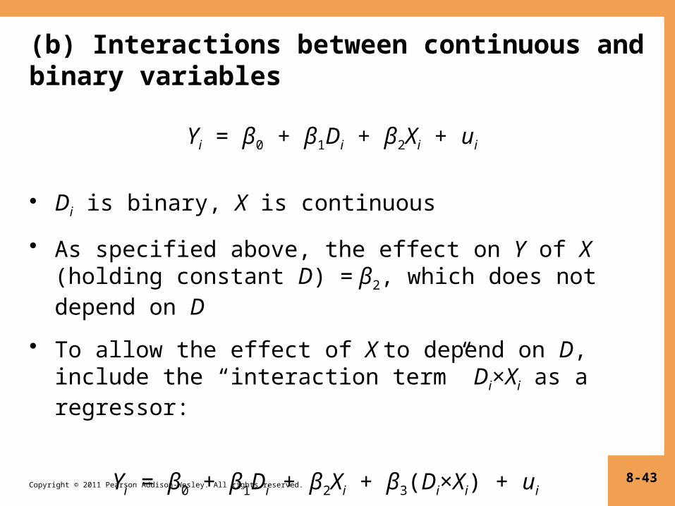
(b) Interactions between continuous and binary variables

Yi = β0 + β1Di + β2Xi + ui

• Di is binary, X is continuous

• As specified above, the effect on Y of X (holding constant D) = β2, which does not depend on D

• To allow the effect of X to depend on D, include the “interaction term” Di×Xi as a regressor:

Yi = β0 + β1Di + β2Xi + β3(Di×Xi) + ui

8-43


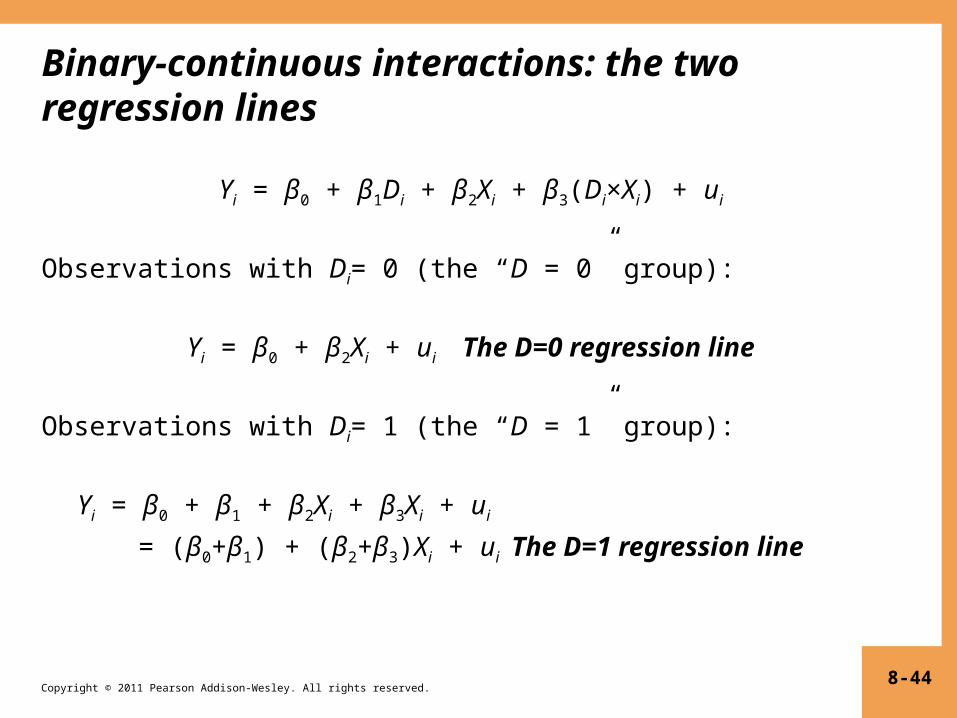
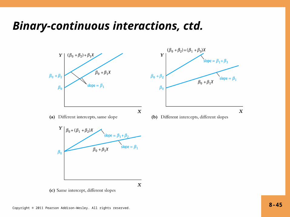
Binary-continuous interactions: the two regression lines


Observations with Di= 0 (the “D = 0” group):

Yi = β0 + β2Xi + ui The D=0 regression line

Observations with Di= 1 (the “D = 1” group):

Yi = β0 + β1 + β2Xi + β3Xi + ui

= (β0+β1) + (β2+β3)Xi + ui The D=1 regression line

8-44


Binary-continuous interactions, ctd.

8-45


Interpreting the coefficients


General rule: compare the various cases

Y = β0 + β1D + β2X + β3(D×X) (b)

Now change X:

Y + ΔY = β0 + β1D + β2(X+ΔX) + β3[D×(X+ΔX)] (a)

subtract (a) – (b):ΔY = β2ΔX + β3DΔX or = β2 + β3D

• The effect of X depends on D (what we wanted) • β3 = increment to the effect of X, when D = 1

8-46

Y

X


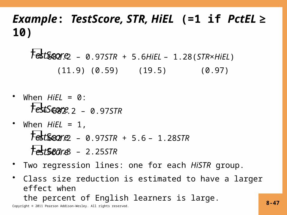
Example: TestScore, STR, HiEL (=1 if PctEL ≥ 10)

= 682.2 – 0.97STR + 5.6HiEL – 1.28(STR×HiEL)

(11.9) (0.59) (19.5) (0.97)

• When HiEL = 0:

= 682.2 – 0.97STR

• When HiEL = 1,

= 682.2 – 0.97STR + 5.6 – 1.28STR

= 687.8 – 2.25STR

• Two regression lines: one for each HiSTR group.

• Class size reduction is estimated to have a larger effect when the percent of English learners is large.

8-47

TestScore

TestScoreTestScore

TestScore


Example, ctd: Testing hypotheses

= 682.2 – 0.97STR + 5.6HiEL – 1.28(STR×HiEL) (11.9) (0.59) (19.5) (0.97)• The two regression lines have the same slope the

coefficient on STR×HiEL is zero: t = –1.28/0.97 = –1.32

• The two regression lines have the same intercept the coefficient on HiEL is zero: t = –5.6/19.5 = 0.29

• The two regression lines are the same population coefficient on HiEL = 0 and population coefficient on STR×HiEL = 0: F = 89.94 (p-value < .001) !!

• We reject the joint hypothesis but neither individual hypothesis (how can this be?)

8-48

TestScore


(c) Interactions between two continuous variables

Yi = β0 + β1X1i + β2X2i + ui

• X1, X2 are continuous

• As specified, the effect of X1 doesn’t depend on X2

• As specified, the effect of X2 doesn’t depend on X1

• To allow the effect of X1 to depend on X2, include the “interaction term” X1i×X2i as a regressor:

Yi = β0 + β1X1i + β2X2i + β3(X1i×X2i) + ui

8-49


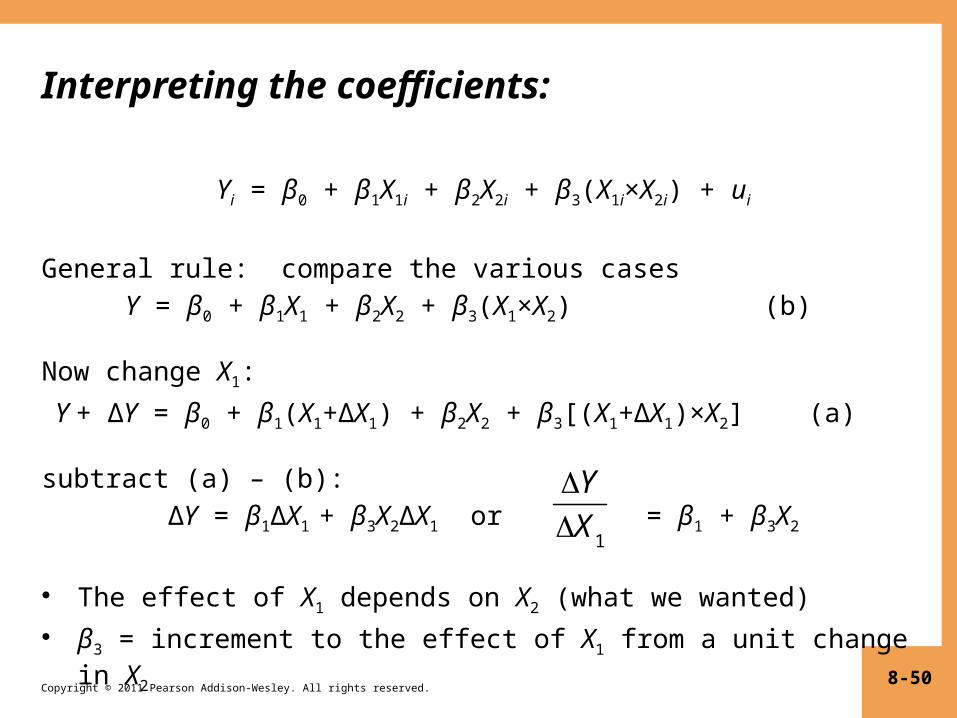
Interpreting the coefficients:

Yi = β0 + β1X1i + β2X2i + β3(X1i×X2i) + ui

General rule: compare the various cases Y = β0 + β1X1 + β2X2 + β3(X1×X2) (b)

Now change X1:

Y + ΔY = β0 + β1(X1+ΔX1) + β2X2 + β3[(X1+ΔX1)×X2] (a)

subtract (a) – (b):ΔY = β1ΔX1 + β3X2ΔX1 or = β1 + β3X2

• The effect of X1 depends on X2 (what we wanted)

• β3 = increment to the effect of X1 from a unit change in X2

8-50

Y

X1


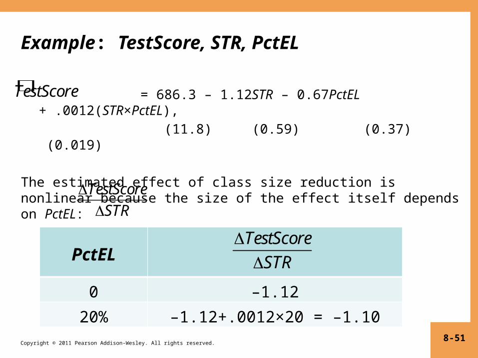
Example: TestScore, STR, PctEL

= 686.3 – 1.12STR – 0.67PctEL + .0012(STR×PctEL), (11.8) (0.59) (0.37) (0.019) The estimated effect of class size reduction is nonlinear because the size of the effect itself depends on PctEL:

= –1.12 + .0012PctEL

8-51

PctEL

0 –1.1220% –1.12+.0012×20 = –1.10

TestScore

STR

TestScore

TestScore

STR


Example, ctd: hypothesis tests

= 686.3 – 1.12STR – 0.67PctEL + .0012(STR×PctEL), (11.8) (0.59) (0.37) (0.019)

• Does population coefficient on STR×PctEL = 0?

t = .0012/.019 = .06 can’t reject null at 5% level

• Does population coefficient on STR = 0?

t = –1.12/0.59 = –1.90 can’t reject null at 5% level

• Do the coefficients on both STR and STR×PctEL = 0?

F = 3.89 (p-value = .021) reject null at 5% level(!!) (Why? high but imperfect multicollinearity)

8-52

TestScore


Application: Nonlinear Effects on Test Scores of the Student-Teacher Ratio (SW Section 8.4)

Nonlinear specifications let us examine more nuanced questions about the Test score – STR relation, such as: 1. Are there nonlinear effects of class size reduction

on test scores? (Does a reduction from 35 to 30 have same effect as a reduction from 20 to 15?)

2. Are there nonlinear interactions between PctEL and STR? (Are small classes more effective when there are many English learners?)

8-53


Strategy for Question #1 (different effects for different STR?)

• Estimate linear and nonlinear functions of STR, holding constant relevant demographic variables– PctEL– Income (remember the nonlinear TestScore-Income

relation!)– LunchPCT (fraction on free/subsidized lunch)

• See whether adding the nonlinear terms makes an “economically important” quantitative difference (“economic” or “real-world” importance is different than statistically significant)

• Test for whether the nonlinear terms are significant

8-54


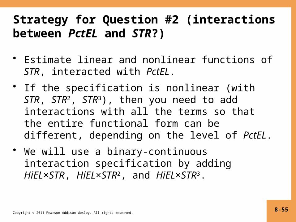
Strategy for Question #2 (interactions between PctEL and STR?)

• Estimate linear and nonlinear functions of STR, interacted with PctEL.

• If the specification is nonlinear (with STR, STR2, STR3), then you need to add interactions with all the terms so that the entire functional form can be different, depending on the level of PctEL.

• We will use a binary-continuous interaction specification by adding HiEL×STR, HiEL×STR2, and HiEL×STR3.

8-55


What is a good “base” specification?

• The TestScore – Income relation:• The logarithmic specification is better behaved near the

extremes of the sample, especially for large values of income.

8-56

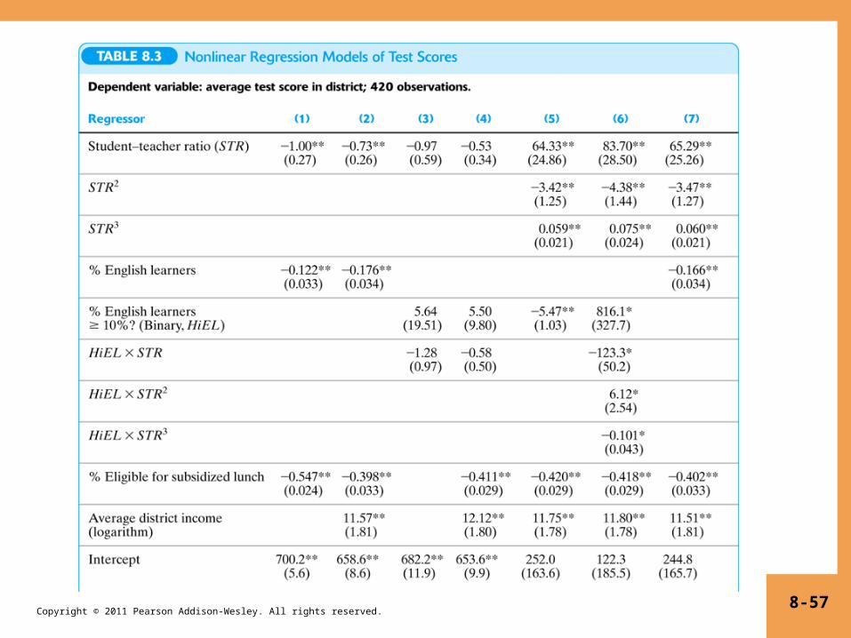
Copyright © 2011 Pearson Addison-Wesley. All rights reserved. 8-57


Tests of joint hypotheses:

What can you conclude about question #1? About question #2?

8-58


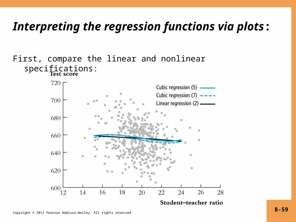
Interpreting the regression functions via plots:

First, compare the linear and nonlinear specifications:

8-59


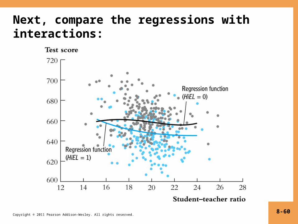
Next, compare the regressions with interactions:

8-60


Summary: Nonlinear Regression Functions

• Using functions of the independent variables such as ln(X) or X1×X2, allows recasting a large family of nonlinear regression functions as multiple regression.

• Estimation and inference proceed in the same way as in the linear multiple regression model.

• Interpretation of the coefficients is model-specific, but the general rule is to compute effects by comparing different cases (different value of the original X’s)

• Many nonlinear specifications are possible, so you must use judgment:

– What nonlinear effect you want to analyze?

– What makes sense in your application?8-61

Documents

Copyright © 2011 Pearson Addison-Wesley. All rights reserved. Nonlinear Regression Functions Chapter 8