Copyright © 2011 by Statistical Innovations Inc. All rights reserved. Ridge Regression: L-2 Penalty Minimize Penalized Least Squares rather than OLS Or

Copyright © 2011 by Statistical Innovations Inc. All rights reserved.

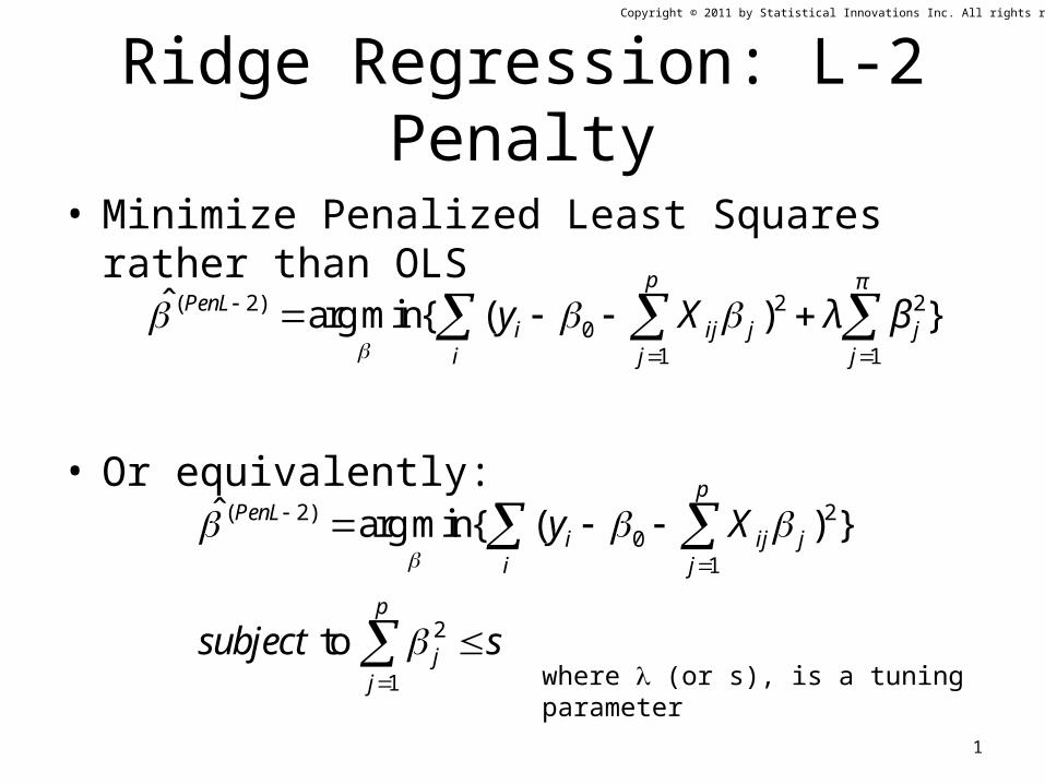
Ridge Regression: L-2 Penalty

• Minimize Penalized Least Squares rather than OLS

• Or equivalently:

( 2) 2 20

1 1

ˆ arg min{ ( ) }p π

PenLi ij j j

i j j

y X λ β

( 2) 20

1

2

1

ˆ arg min{ ( ) }

to

pPenL

i ij ji j

p

jj

y X

subject s

where (or s), is a tuning parameter

1


Lasso: L-1 Penalty

• Penalize by sum of absolute values

20

1

1

ˆ arg min{ ( ) }

to | |

plasso

i ij ji j

p

j

y X

subject s

Advantage over L-2 is Sparseness – built in feature selection

( 1) 20

1 1

ˆ arg min{ ( ) }p π

PenLi ij j

i j j

y X λ

Or equivalently:

2


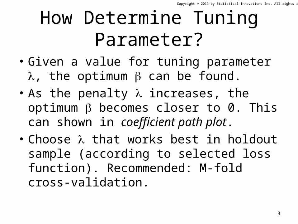
How Determine Tuning Parameter?

• Given a value for tuning parameter , the optimum can be found.

• As the penalty increases, the optimum becomes closer to 0. This can shown in coefficient path plot.

• Choose that works best in holdout sample (according to selected loss function). Recommended: M-fold cross-validation.

3


Coefficient Path Plot for Ridge Regression

4

As the penalty is increased, shown right to left on the x-axis, the coefficients shrink towards 0. For any given penalty, all coefficients are non-zero.


Coefficient Path Plot for Lasso Shows Sparse Solutions Similar to Step-wise Regression

5

With the largest penalty, all coefficients are 0. As the penalty is reduced the predictors begin to enter into the equation.

RP5 enters 1st ABL1 enters 2nd

CD97 and BRCA1 enter 3rd SP1 and MYC enter nextTNF enters next, followed by IQGAP1


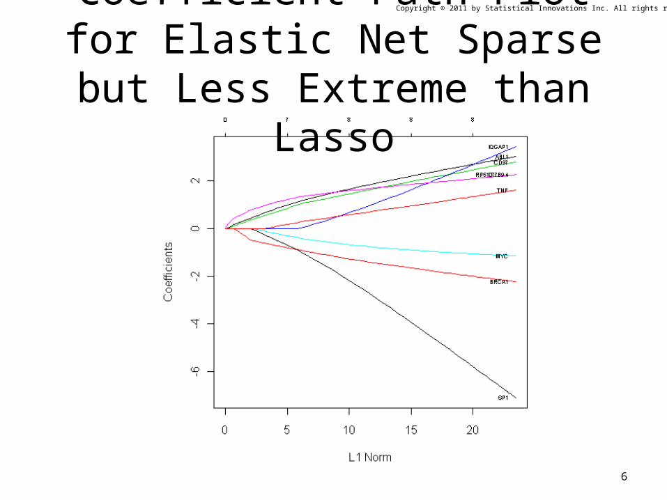
Coefficient Path Plot for Elastic Net Sparse but Less Extreme than Lasso

6


For Comparison: Coefficient Path Plot for CCR (to be Described Later)

7


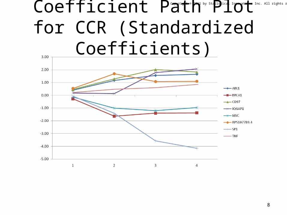
Coefficient Path Plot for CCR (Standardized Coefficients)

8


Using Derived Inputs

• Goal: Using linear combinations of predictors (Xs) as inputs in the regression

• Usually the derived inputs are orthogonal to each other

• Principal component regression– Get K components using SVD

9


Approaches based on Principal Component Analysis (PCA)

1) Principal Component Regression (PCR) – Transform the predictors X1, X2, …, XP to principal components, S1, S2, …, SP, each component defined as a weighted sum of all the predictors. Then use the top K < P components (those explaining the most predictor variance) as predictors in the model.

• Advantages over stepwise regression:• PCR takes into account information on more predictors. There may be only K<P predictors in model, but each component incorporates information on multiple X variables, thus possibly providing better prediction of Z.• Since components are orthogonal (uncorrelated), problem due to multicolinearity goes away.

• Disadvantages over stepwise regression: • The components are not necessarily predictive of Z and thus may not provide better prediction of Z than stepwise regression.• To apply the model, one needs measurements of all P of the X variables.• Solution depends upon whether predictors are standardized (analysis of correlation matrix) or unstandardized (analysis of covariance matrix)

2) Supervised PCR (Bair, et. al., 2006) – Rather than the first K components, select only the K components that are significant predictors of Z

• Advantage over PCR – Each component is assured to be predictive of Z.• Disadvantage: Excludes components that act as suppressor variables, thus providing poorer prediction than PLS regression and Correlated Component Regression.• Non-sparse: To apply the model, one needs measurements on all P of the X variables.

10


Principal Components Regression (PCR)

• The Researcher wants to understand how Z relates to the Xs, not how Z relates to the components.

• However, since each component is a weighted sum of the Xs, substituting for the components, one gets coefficients for the Xs.Example with 2 Components:

11

1.2 1 2.1 2( )Logit Z b S b S 1 .11

P

g gg

S X

2 .21

P

g gg

S X

1.2 .1 2.1 .21

( ) ( )P

g g gg

Logit Z b b X

Note: If the components are meaningful (as in CCR), the coefficients of the Xs can be meaningful


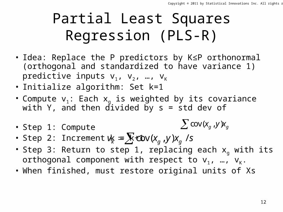
Partial Least Squares Regression (PLS-R)

• Idea: Replace the P predictors by K≤P orthonormal (orthogonal and standardized to have variance 1) predictive inputs v1, v2, …, vK

• Initialize algorithm: Set k=1• Compute v1: Each xg is weighted by its covariance with Y, and

then divided by s = std dev of • Step 1: Compute • Step 2: Increment k = k+1• Step 3: Return to step 1, replacing each xg with its orthogonal

component with respect to v1, …, vK.• When finished, must restore original units of Xs

cov( , ) /k g gv x y x s

12

cov( , )g gx y x


Correlated Component Regression (CCR)

New methods are presented that extend traditional regression modeling to apply to high dimensional data where the number of predictors P exceeds the number of cases N (P >> N). The general approach yields K correlated components, weights associated with the first component providing direct effects for the predictors, and each additional component providing improved prediction by including suppressor variables and otherwise updating effect estimates. The proposed approach, called Correlated Component Regression (CCR), involves sequential application of the Naïve Bayes rule.

With high dimensional data (small samples and many predictors) it has been shown that use of the Naïve Bayes Rule:

“greatly outperforms the Fisher linear discriminant rule (LDA) under broad conditions when the number of variables grows faster than the number of observations”, Bickel and Levina (2004)

even when the true model is that of LDA! Results from simulated and real data suggest that CCR outperforms other sparse regression methods, with generally good outside-the-sample prediction attainable with K=2, 3, or 4.

When P is very large, an initial CCR-based variable selection step is also proposed.

13


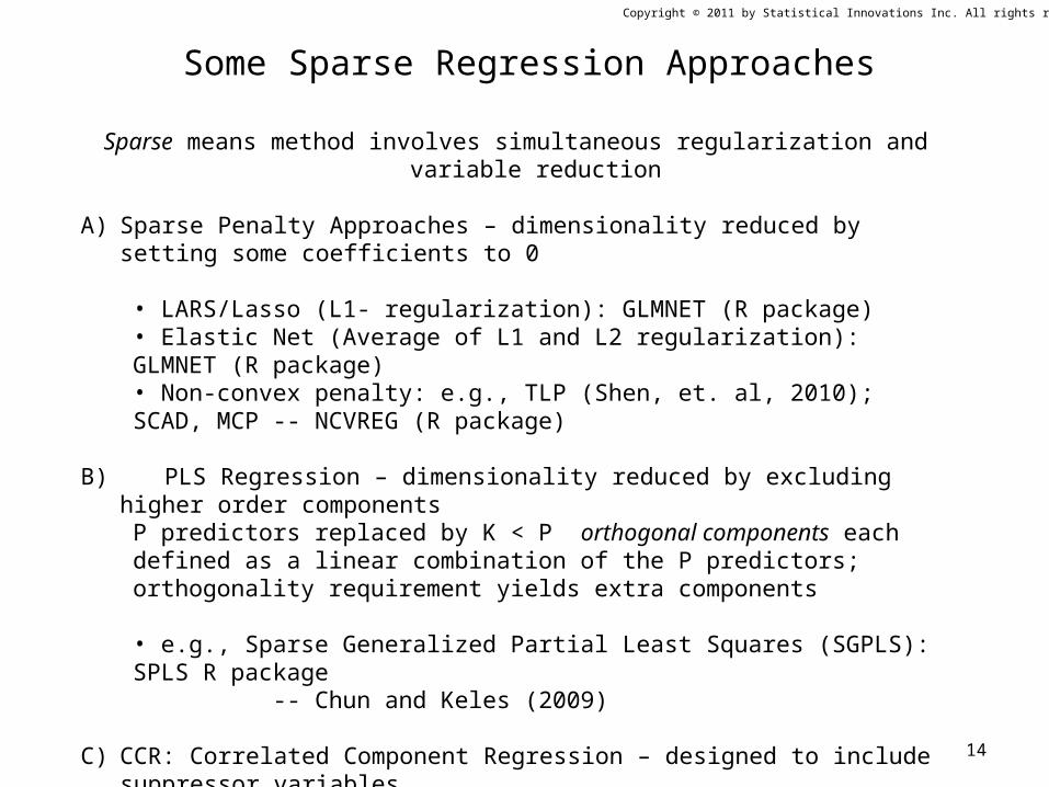
Some Sparse Regression Approaches

14

Sparse means method involves simultaneous regularization and variable reduction

A) Sparse Penalty Approaches – dimensionality reduced by setting some coefficients to 0

• LARS/Lasso (L1- regularization): GLMNET (R package)• Elastic Net (Average of L1 and L2 regularization): GLMNET (R package)• Non-convex penalty: e.g., TLP (Shen, et. al, 2010); SCAD, MCP -- NCVREG (R package)

B) PLS Regression – dimensionality reduced by excluding higher order componentsP predictors replaced by K < P orthogonal components each defined as a linear combination of the P predictors; orthogonality requirement yields extra components

• e.g., Sparse Generalized Partial Least Squares (SGPLS): SPLS R package -- Chun and Keles (2009)

C) CCR: Correlated Component Regression – designed to include suppressor variablesP predictors replaced by K < P correlated components each defined as a linear combination of the P (or a subset of the P) predictors: CORExpress™ program

-- Magidson (2010)


Correlated Component Regression Approach*

15

Correlated Component Regression (CCR) utilizes K correlated components, each a linear combination of the predictors, to predict an outcome variable.

• The first component S1 captures the effects of prime predictors which have direct effects on the outcome. It is a weighted average of all 1-predictor effects.

• The second component S2, correlated with S1, captures the effects of suppressor variables (proxy predictors) that improve prediction by removing extraneous variation from one or more prime predictors. Suppressor variables will be examined in more detail in Session 3.

• Additional components are included if they improve prediction significantly.

Prime predictors are identified as those having significant loadings on S1, and proxy predictors as those having significant loadings on S2, and non-significant loadings on component #1.

• Simultaneous variable reduction is achieved using a step-down algorithm where at each step the least important predictor is removed, importance defined by the absolute value of the standardized coefficient. K-fold cross-validation is used to determine the number of components and predictors.

*Multiple patent applications are pending regarding this technology


Example: Correlated Component Regression Estimation Algorithmas Applied to Predictors in Logistic Regression: CCR-Logistic

16

Step 1: Form 1st component S1 as average of P 1-predictor models (ignoring g)

g=1,2,…,P;

1-component model:

Step 2: Form 2nd component S2 as average of Where each is estimated from the following 2-predictor logit model:

g=1,2,…,P;

Step 3: Estimate the 2-component model using S1 and S2 as predictors:

Continue for K = 3,4,…,K*-component model. For example, for K=3, step 2 becomes:

.1g gX1( )Logit Z S

.1 1 .1( ) g g gLogit Z S X

.1g

( ) g g gLogit Z X

1.2 1 2.1 2( )Logit Z b S b S

.12 .1 1 .2 2 .12( ) g g g gLogit Z S S X

2 .11

1 P

g gg

S XP

11

1 P

g gg

S XP


Other CCR Variants

17

1) Linear Discriminant Analysis: CCR-LDAUtilize the random X normality assumption to speed up algorithm.In step K, regress each predictor on Z, controlling for S1,…,SK-1 in fast linear regressions:

e.g., for K=1: g=1,2,…,P;'

g g gX Z 11

1 P

g gg

S XP

' /g g MSE

2) Ordinal Logistic Regression: CCR-Logist, CCR-LDA (extended to ordinal dependent)For ordinal, Z categories takes on numeric scores (Magidson, 1996)

3) Survival Analysis: CCR-Cox – Model expressed as Poisson Regressions (Vermunt, 2009)

4) Linear Regression: CCR-LM – for improved efficiency, in step K each predictor is regressed on Z (single application of multivariate linear regression, controlling for S1,…,SK-1)

where g is maximum likelihood estimate for log-odds ratio in simple logistic regression model (Lyles et. al., 2009)

For K-component CCR-LDA model, perform LDA using the components S1, S2, …, SK in place of the X-variables. For K=P, get equivalent to LDA!


Correlated Component Regression Step-down Variable Reduction Step

18

Step Down: For user-specified K*, eliminate the variable that is least important in K*-component model, where importance is quantified by the absolute value of the variable’s standardized coefficient, the standardized coefficient being defined by:

Example with K*=2.

Comparing absolute value of standardized coefficients for the K*=2-component model determines predictor g* to be least important. Then exclude that predictor and repeat the steps of the CCR estimation algorithm on the reduced set of predictors.

In practice, for large P, more than 1 predictor can be eliminated at a time. For example, at each step we can eliminate the 1% of the predictors that are least important until P < 100, at which time we can begin eliminating 1 predictor at a time. This process can continue until 1 predictor remains. Note that for P = K, the model becomes ‘saturated’ and is equivalent to the traditional regression model. In order to reduce the number of predictors further, we maintain the saturated model by reducing K so that P = K. Thus, for example, for K = 4, when we step down to 3 predictors, we reduce K so K = 3.

*g g g


Correlated Component Regression Step-down Variable Reduction Step

19

M-fold cross-validation is used to determine the optimal value for the tuning parameters K and P for a given criterion (or loss function). For computational efficiency, this is done first for K=1 components, then K=2 components, ... , up through say K=10 components. Since in practice, the optimal number of components will rarely be greater than 10, one can be fairly sure of obtaining a good model with K < 11. For a given number of components K, the optimal number of predictors P*(K), can then be determined, and (P*, K*) can be determined as the combination minimizing the loss function. Thus, P* predictors will be retained where P* is the best of the P*(K), K=1,..., 10, and K* will be the optimal number of components associated with P* predictors.

Evaluating up to only 10 components saves computer resources since the speed of CCR increases exponentially as the number of components increases. Since estimation utilizes a sequential process, most of the sufficient statistics from previous runs can be reused. Hence, CCR is very fast with a small number of components.

Let A(K) = cross-validated accuracy for the K-component model based on the optimal number of predictors P*(K). Then, if A(1) < A(2) < A(3) < A(4) > A(5), we might stop after evaluating K = 5 and not evaluate K=6,7,8, saving more computer time. That is, if the 5-component model fails to provide a solution that improves over the 4-component model according to the results of the M-fold cross-validation, we might take K* = 4, and P* = P*(4). As a somewhat more conservative approach, we might also evaluate K = 6 to check that performance continues to degrade.

The use of M-fold cross-validation to determine the optimal value for one or more 'tuning parameters' is standard practice in data mining. It is used for example, to obtain the single tuning parameter 'lambda' in the lasso penalized regression approach. Here, we use it to optimize the two tuning parameters, P and K. We do it in an efficient way by doing it for each component separately, and evaluate only a small number of models (those with K in a specified range), and limit to small values of K. In practice with high-dimensional data, we have found that the best model is rarely one with K>10.


ReferencesBair, E., T. Hastie, P. Debashis, and R. Tibshirani (2006). Prediction by supervised principal components. Journal of the American Statistical Association 101, 119–137.

Bickel and Levina (2004). Some theory for Fisher’s linear discriminant function, ‘naive Bayes’, and some alternatives when there are many more variables than observations, Bernoulli 10(6), 989-1010.

Fan, J. and Li, R. (2001). Variable selection via nonconcave penalized likelihood and its oracle properties. Journal of the American Statistical Association, 96, 1348-1360.

Fan, J. and J. Lv (2008). Sure Independence Screening for Ultra-High Dimensional Feature Space (with Addendum), Journal of the Royal Statistical Society: Series B (Statistical Methodology), Volume 70, Issue 5, pages 849–911, November.

Fort, G. and Lambert-Lacroix, S. (2003). Classification Using Partial Least Squares with Penalized Logistic Regression. IAP-Statistics, TR0331.

Friedman, L. and M. Wall (2005). Graphical Views Of Suppression and Mutlicollinearity In Multiple Linear Regression. American Statistician, May 2005. Vol 59, No. 2, pp 127-136.

Friedman, J., T. Hastie, and R. Tibshirani (2010). Regularization Paths for Generalized Linear Models via Coordinate Descent. Journal of Statistical Software, 33(1), 1-22.

Horst, P. (1941). The role of predictor variables which are independent of the criterion. Social Science Research Bulletin, 48, 431 436.‑

Hyonho, C. and S. Keleş (2009). Sparse partial least squares regression for simultaneous dimension reduction and variable selection. University of Wisconsin, Madison, USA.

20


References (continued)Lynn, H. (2003). Suppression and Confounding in Action. The American Statistician, Vol.57, 2003.

Lyles R.H., Y. Guo and A. Hill (2009). “A Fresh Look at the Discrimination Function Approach for Estimating Crude or Adjusted Odds Ratios”, The American Statistician, Vol 63, No. 4 (November ), pp 320-327.

Magidson, J. (2010). User’s Guide for CORExpress. Belmont MA: Statistical Innovations Inc.

Magidson, J. (1996). “Maximum Likelihood Assessment of Clinical Trials Based on an Ordered Categorical Response.“, Drug Information Journal, Maple Glen, PA: Drug Information Association, Vol. 30, No. 1, 143-170.

Magidson, J. (2010). A Fast Parsimonious Maximum Likelihood Approach for Prediction Outcome Variables from a Large Number of Predictors. COMPSTAT 2010 Proceedings. Forthcoming.

Magidson, J., and K. Wassmann, (2010) “The Role of Proxy Genes in Predictive Models: An Application to Early Detection of Prostate Cancer”, Proceedings of the American Statistical Association.

Magidson, J. and Y. Yuan (2010) “Comparison of Results of Various Methods for Sparse Regression and Variable Pre-Screening”, unpublished report #CCR2010.1, Belmont MA: Statistical Innovations.

Shen, X., Pan, W., Zhu, Y., and Zhou, H. (2010). “On L0 regularization in high-dimensional regression”, to appear.

Vermunt, J.K. (2009): Event history analysis. in R. Millsap (ed.) Handbook of Quantitative Methods in Psychology, 658-674. London: Sage.

Wyman, P. and J. Magidson (2008). The Effect of the Enneagram on Measurement of MBTI® Extraversion-Introversion Dimension. The Journal of Psychological Type, Volume 68, Issue 1 (January).

Zou, H. and Hastie, T. (2005). Regularization and variable selection via the elastic net. J. Roy. Statist. Soc. Ser. B 67, 301-320.

21

Documents

Copyright © 2011 by Statistical Innovations Inc. All rights reserved. Ridge Regression: L-2 Penalty Minimize Penalized Least Squares rather than OLS Or