Copyright © 2009 Pearson Education, Inc.

Chapter 14

From Randomness to Probability

Slide 1- 3Copyright © 2009 Pearson Education, Inc.

Dealing with Random Phenomena

A random phenomenon is a situation in which we know what outcomes could happen, but we don’t know which particular outcome did or will happen.

In general, each occasion upon which we observe a random phenomenon is called a trial.

At each trial, we note the value of the random phenomenon, and call it an outcome.

When we combine outcomes, the resulting combination is an event.

The collection of all possible outcomes is called the sample space.

Slide 1- 4Copyright © 2009 Pearson Education, Inc.

First a definition . . . When thinking about what happens with

combinations of outcomes, things are simplified if the individual trials are independent. Roughly speaking, this means that the

outcome of one trial doesn’t influence or change the outcome of another.

For example, coin flips are independent.

The Law of Large Numbers

Slide 1- 5Copyright © 2009 Pearson Education, Inc.

The Law of Large Numbers (cont.)

The Law of Large Numbers (LLN) says that the long-run relative frequency of repeated independent events gets closer and closer to a single value.

We call the single value the probability of the event.

Because this definition is based on repeatedly observing the event’s outcome, this definition of probability is often called empirical probability.

Slide 1- 6Copyright © 2009 Pearson Education, Inc.

The Nonexistent Law of Averages

The LLN says nothing about short-run behavior. Relative frequencies even out only in the long

run, and this long run is really long (infinitely long, in fact).

The so called Law of Averages (that an outcome of a random event that hasn’t occurred in many trials is “due” to occur) doesn’t exist at all.

Slide 1- 7Copyright © 2009 Pearson Education, Inc.

Modeling Probability

When probability was first studied, a group of French mathematicians looked at games of chance in which all the possible outcomes were equally likely. It’s equally likely to get any one of six outcomes from

the roll of a fair die. It’s equally likely to get heads or tails from the toss of a

fair coin. However, keep in mind that events are not always equally

likely. A skilled basketball player has a better than 50-50

chance of making a free throw.

Slide 1- 8Copyright © 2009 Pearson Education, Inc.

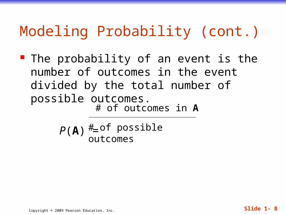
The probability of an event is the number of outcomes in the event divided by the total number of possible outcomes.

P(A) =

Modeling Probability (cont.)

# of outcomes in A

# of possible outcomes

Slide 1- 9Copyright © 2009 Pearson Education, Inc.

Personal Probability

In everyday speech, when we express a degree of uncertainty without basing it on long-run relative frequencies or mathematical models, we are stating subjective or personal probabilities.

Personal probabilities don’t display the kind of consistency that we will need probabilities to have, so we’ll stick with formally defined probabilities.

Slide 1- 10Copyright © 2009 Pearson Education, Inc.

The First Three Rules of Working with Probability

We are dealing with probabilities now, not data, but the three rules don’t change. Make a picture. Make a picture. Make a picture.

Slide 1- 11Copyright © 2009 Pearson Education, Inc.

The First Three Rules of Working with Probability (cont.)

The most common kind of picture to make is called a Venn diagram.

We will see Venn diagrams in practice shortly…

Slide 1- 12Copyright © 2009 Pearson Education, Inc.

Formal Probability

1. Two requirements for a probability: A probability is a number between 0 and 1. For any event A, 0 ≤ P(A) ≤ 1.

Slide 1- 13Copyright © 2009 Pearson Education, Inc.

Formal Probability (cont.)

2. Probability Assignment Rule: The probability of the set of all possible

outcomes of a trial must be 1. P(S) = 1 (S represents the set of all possible

outcomes.)

Slide 1- 14Copyright © 2009 Pearson Education, Inc.

Formal Probability (cont.)

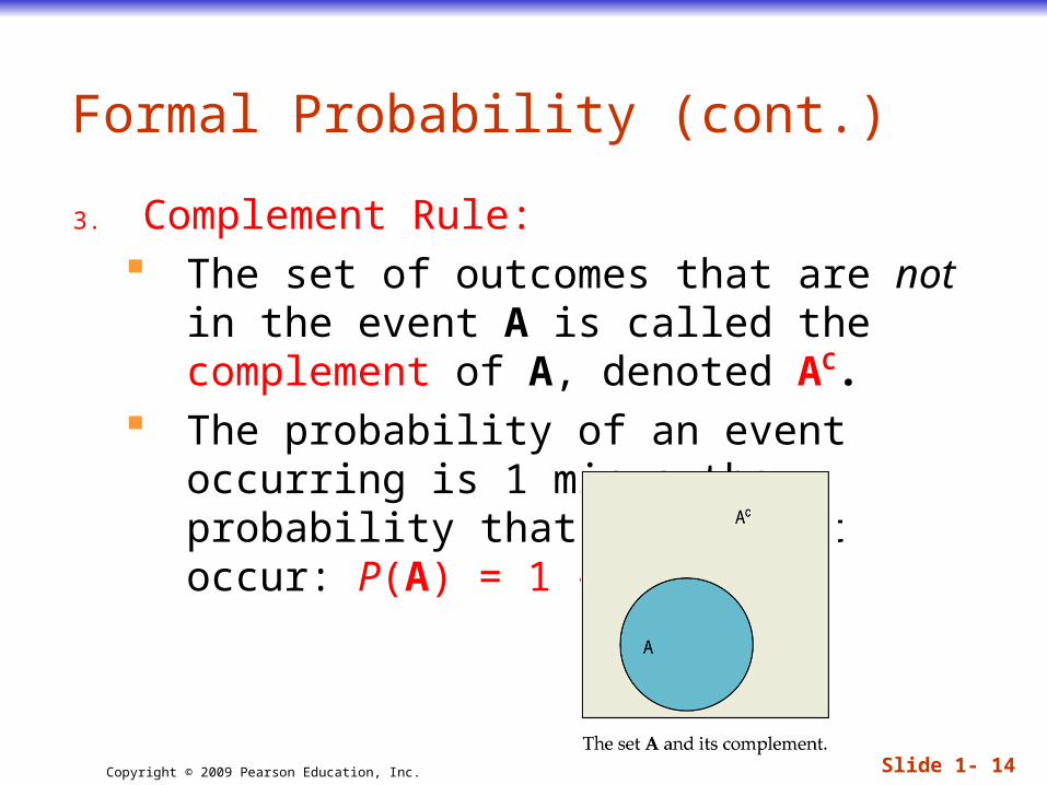
3. Complement Rule: The set of outcomes that are not in the event

A is called the complement of A, denoted AC. The probability of an event occurring is 1

minus the probability that it doesn’t occur: P(A) = 1 – P(AC)

Slide 1- 15Copyright © 2009 Pearson Education, Inc.

Formal Probability (cont.)

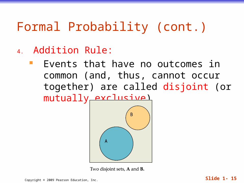
4. Addition Rule: Events that have no outcomes in common

(and, thus, cannot occur together) are called disjoint (or mutually exclusive).

Slide 1- 16Copyright © 2009 Pearson Education, Inc.

Formal Probability (cont.)

4. Addition Rule (cont.): For two disjoint events A and B, the

probability that one or the other occurs is the sum of the probabilities of the two events.

P(A or B) = P(A) + P(B), provided that A and B are disjoint.

Slide 1- 17Copyright © 2009 Pearson Education, Inc.

Formal Probability

5. Multiplication Rule (cont.): For two independent events A and B, the

probability that both A and B occur is the product of the probabilities of the two events.

P(A and B) = P(A) x P(B), provided that A and B are independent.

Slide 1- 18Copyright © 2009 Pearson Education, Inc.

Formal Probability (cont.)

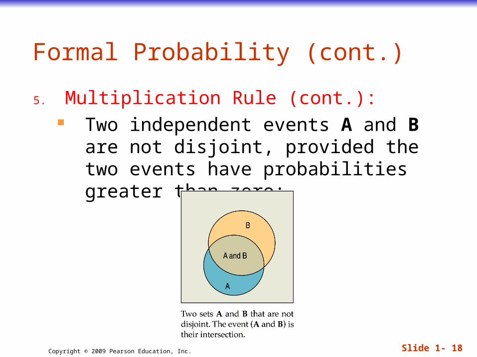
5. Multiplication Rule (cont.): Two independent events A and B are not

disjoint, provided the two events have probabilities greater than zero:

Slide 1- 19Copyright © 2009 Pearson Education, Inc.

Formal Probability (cont.)

5. Multiplication Rule: Many Statistics methods require an

Independence Assumption, but assuming independence doesn’t make it true.

Always Think about whether that assumption is reasonable before using the Multiplication Rule.

Slide 1- 20Copyright © 2009 Pearson Education, Inc.

Formal Probability - Notation

Notation alert: In this text we use the notation P(A or B) and

P(A and B). In other situations, you might see the following:

P(A B) instead of P(A or B) P(A B) instead of P(A and B)

Slide 1- 21Copyright © 2009 Pearson Education, Inc.

Putting the Rules to Work

In most situations where we want to find a probability, we’ll often use the rules in combination.

A good thing to remember is that sometimes it can be easier to work with the complement of the event we’re really interested in.

Slide 1- 22Copyright © 2009 Pearson Education, Inc.

What Can Go Wrong?

Beware of probabilities that don’t add up to 1. To be a legitimate probability assignment, the

sum of the probabilities for all possible outcomes must total 1.

Don’t add probabilities of events if they’re not disjoint. Events must be disjoint to use the Addition

Rule.

Slide 1- 23Copyright © 2009 Pearson Education, Inc.

What Can Go Wrong? (cont.)

Don’t multiply probabilities of events if they’re not independent. The multiplication of probabilities of events that

are not independent is one of the most common errors people make in dealing with probabilities.

Don’t confuse disjoint and independent—disjoint events can’t be independent.

Slide 1- 24Copyright © 2009 Pearson Education, Inc.

What have we learned?

Probability is based on long-run relative frequencies.

The Law of Large Numbers speaks only of long-run behavior. Watch out for misinterpreting the LLN.

Slide 1- 25Copyright © 2009 Pearson Education, Inc.

What have we learned? (cont.)

There are some basic rules for combining probabilities of outcomes to find probabilities of more complex events. We have the: Probability Assignment Rule Complement Rule Addition Rule for disjoint events Multiplication Rule for independent events