Embed Size (px)
Citation preview

Copyright © 1993, by the author(s).
All rights reserved.
Permission to make digital or hard copies of all or part of this work for personal or
classroom use is granted without fee provided that copies are not made or distributed
for profit or commercial advantage and that copies bear this notice and the full citation
on the first page. To copy otherwise, to republish, to post on servers or to redistribute to
lists, requires prior specific permission.

MULTIPROCESSOR DSP CODE SYNTHESIS
IN PTOLEMY
by
Praveen Kumar Murthy
Memorandum No. UCB/ERL M93/66
30 August 1993

MULTIPROCESSOR DSP CODE SYNTHESIS
IN PTOLEMY
by
Praveen Kumar Murthy
Memorandum No. UCB/ERL M93/66
30 August 1993
ELECTRONICS RESEARCH LABORATORY
College of EngineeringUniversity of California, Berkeley
94720

MULTIPROCESSOR DSP CODE SYNTHESIS
IN PTOLEMY
by
Praveen Kumar Murthy
Memorandum No. UCB/ERL M93/66
30 August 1993
ELECTRONICS RESEARCH LABORATORY
College of EngineeringUniversity of California, Berkeley
94720

1 Abstract 1
2 Introduction 2
2.1 Overview of Ptolemy. 32.2 Synchronous Dataflow 4
3 TheSprocDSP 43.1 The Central MemoryUnit 53.2 The General Signal Processors 63.3 The Data Row Managers 73.4 The board 7
3.5 The Sproc development system 83.5.1 SSIMD scheduling 83.5.2 The IPC vocoder 93.5.2.1An upper bound for ao(0) 15
4 Code Generation in Ptolemy 174.1 Stars 18
4.2 Targets 234.3 Schedulers 24
4.4 Interprocessor communication 254.4.1 Send/Receive 254.4.2 Spread/Collect 25
5 The Sproc domain 265.1 SprocTarget 27
5.1.1 Send/Receive 30
5.1.2 Memory Allocation 325.1.3 I/O 33
5.1.3.1Apossibilityforfuture work 345.2 Other Targets 345.3 Some examples 35
5.3.1 Plucked strings 355.3.2 QMF Filter bank 365.3.3 ADPCM coding of speech 39
6 Conclusion 41
7 Acknowledgments 41
8 References 42
Appendix: Code for QMF filter bank 44
10f1

*OT*mmnw«a»ew»OTi«miwft«
1 Abstract
miiiiiifiiiiiiimnniiiniriTiiiiiiiiiiiNiiiii
Ptolemy is a flexible tool that has been developed for simulation, prototyping, and soft
ware synthesis for large heterogenous systems. The objectives of Ptolemy encompass virtually all
aspects of designing signal processing and communication systems, ranging from algorithms and
communication strategies, through simulation, parallel computing, and generation of real-time
prototypes. This project report describes the multiprocessor code synthesis aspect ofPtolemy, and
in particular, code synthesis for the Sproc digital signal processor (DSP) made by Star Semiconductor.
1of46

2 of 46
Introduction
The reality with most high-performance DSP chips is that they are very tedious and com
plex to program. In addition, programming parallel DSP architectures has required adaptation of
algorithms to parallel implementations on a case-by-case basis, with each application being care
fully analyzed for concurrency. The bulk of coding for DSPs is done using assembly language
techniques and requires the programmer to be familiar with many details of the chips architecture,
such as pipelines. Although C compilers exist for many popularDSPs, they produce code that is
4-5 times less efficient than hand-assembled code and thus are not a feasible solution for demand
ing DSP tasks. The problem with high level language compilers is that they are often not able to
use specialized addressing modes (like bit-reversed addressing for FFT's, hardware support for
circular buffers) efficiently. Another option is to use anapplicative language like Silageto specify
DSPprograms [Gen90]. The declarative semantics of the language, and its support for fixed-point
arithmetic, makes highly efficient code-generation possible. The Mentor/EDC DSPstation is
based on Silage [Men92].
Neither assembly language nor C coding are the most natural ways of specifying DSP
algorithms. A more natural method is to use block diagrams and signal flow graphs [Mes84]. In
this approach, any complete system design methodology must includesoftware synthesis from the
high level block diagram of the system. This can be done by having hand written assembly code
segments in the individual blocks. The hope is that such blocks will be stored in standard libraries
rendering them modular, reusable software components. Software synthesis then consists of two
phases: scheduling and code generation. During the scheduling phase, the blocks are partitioned
onto parallel processors, and for each processor, a sequence of block invocations is determined.
Code generation consists of piecing together the assembly code segments from the blocks in the
order determined by the scheduler. This methodology seems tobeapopular one and is being used
commercially in the Star Semiconductor Sproc system [SS92], in the Comdisco DPC system
[Pow92], and in the CADIS Descartes system.
Introduction

Introduction
2.1 Overview of Ptolemy.
Ptolemy is a software tool that has been developed atBerkeley to facilitate the simulation
oflarge heterogenous systems, for example, communication networks and signal processing systems [Buc93][Alm92], and isbased on dataflow semantics [Den80]. Heterogenous computational
models are achieved through the domain abstraction which enables each subsystem tobe modeled
in away that is natural and efficient for that subsystem. Combination of these heterogenous sub
systems is enabled by the definition of astandard interface called the event horizon. Ptolemy isimplemented in C++ and uses object oriented programming (OOP) methodology to achieveextensibility to new domains without the need to modify or understand existing ones.
The basic unit of modularity in Ptolemy is the Block. A Block contains a method called
go () whose action can be different depending on the model of computation used. In the code
generation domains, this method synthesizes code for the target processor. Its invocation is
directed by aScheduler (another modular object) which, in the case of the synchronous dataflow
(SDF) model of computation, determines the order of firing of the Blocks at compile time.
Another type of object called the Target, describes the specific features ofatarget for code gener
ation. An interconnected block diagram constitutes the user-interface view of the system (or universe). For anexample, see figure 20 at theendof thereport.
There are many domains in Ptolemy, including synchronous dataflow (SDF), discrete
event (DE), and dynamic dataflow (DDF). Of chiefinterest for this project was the SDF domain
since that is the model of computation for which the code generation capability has been com
pletelydeveloped. By model of computation, we mean the operational semantics and the schedul
ing strategy that are usedin simulating computations in that domain. For example, the DEdomain
has a different model of computation than SDF because in the DE domain, the notion of time is
very important, whereas inSDF, time isnot an issue. For DE stars, the management of timestamps
(which indicate the precise time at which the corresponding data was generated) is as important as
the functionality of the star. Theorder inwhich events are generated can benon-deterministic (for
example, queueing networks); hence, we cannot do static scheduling in DE and have to do sched
uling dynamically. Therefore, the operational semantics and scheduling strategy used for DE is
different from that of SDF; werefer tothese two as having different models of computation.
3 of 46

The Sproc DSP
While the domain abstraction is primarily for mixing different models ofcomputation, in
the code generation domains, different domains can have the same model ofcomputation but distinct target languages. For example, Blocks that generate Sproc assembly code using the SDFmodel of computation form their own domain, separate from Blocks that generate Motorola
56000 code using SDF. As an example ofhow Blocks, Targets, and Schedulers can interact, con
sider aset ofBlocks in the Sproc domain. Any of several targets can be chosen including one thatgenerates code in a higher level form consisting of statements containing Block names and
parameters instead of in-line assembly code. Any of two schedulers, each of which uses different
heuristics to obtain parallel schedules, can also be chosen.
2.2 Synchronous Dataflow
Synchronous Dataflow is a special case ofdataflow in which algorithms are described as
directed graphs where the number of samples produced and consumed by each actor on each
invocation is fixed and known at compile time [Lee86][Lee87]. This model is appropriate for signal processing because alarge set of DSP algorithms are easily specified under the SDF paradigm.Advantages of SDF over dataflow are agreater degree of setup-time syntax checking (since sample-rate inconsistencies which can cause deadlock can easily be detected), and run-time efficiency(since the schedules generated are fully static rather than dynamic). In addition, this model
exposes the inherent concurrency in an algorithm that can be exploited in parallel hardware[Sih91].
3 The Sproc DSP
The Sproc signal processing chip is a multiprocessor DSP made by Star Semiconductor[SS92]. The architecture uses fixed point arithmetic and has 16 bit address paths and 24 bit datapaths. There are four so called general signal processors (GSPs) on the chip and these share acentral multi-ported program and data memory unit (fig. 1). Contention for memory is eliminated bygiving access to each GSP in atime division multiplexed manner. Input/output data flow managers (DFMs) coordinate simultaneous data streams, serial channels interface signals, and parallel
4 of 46

The Sproc DSP
Parallel PortMicroprocessorInterface
Access Portfor developmentsystem
Fig 1.Sproc central memory architecture
interfaces enable connections to external processors. The use of time division multiplexed memory and the DFMs eliminates the need for interrupts to handle multiple data streams.
3.1 The Central Memory Unit
The CMU uses a frame composed of time slots, or memory access periods, allotted for
each GSP and for the I/O. The basic frame represents one Sproc chip machine cycle (five master
clock cycles) and includes five time slots of one master clock cycle each (fig. 2). Time slots 1
through 4are used by the GSPs. During time slot 1, GSP 1can read or write the CMU; during slot
2, GSP 2can read or write and so on. Time slot 5is used by I/O operations. It is submultiplexedinto 8divisions for parallel I/O and other operations. During every other machine cycle, slot 5 is
used bythe parallel port and can support signal or data flow without interrupting the processing of
5 of 46

The Sproc DSP
any of the GSPs. During the other machine cycle, slot 5 supports the serial ports, the access port,
and the on- chip probing port.
1 machine cycle (5 clock cycles)
SlotlGSPl
Slot 2GSP 2
Slot 3GSP 3
Slot 4GSP 4
Slot 5I/O
Fig 2. CMU Time Slot Divisions
3.2 The General Signal Processors
The GSPs are 24-bit fixed-point processors and have Harvard-like architectures having
separate programand databuses. The word widths for both program anddataare24 bits, although
some registers are narrower. There are 5 subcycles within each GSP machine cycle (correspond
ing to each clock cycle). These are instruction fetch, decode, data fetch, and two cycles for the
execute phase (fig. 3). All instructions except two execute in one machine cycle, the two excep
tions being the multiply and multiply-and-accumulate instructions, where the result is available
on the third machine cycle. However, non-multiply instructions can be executed while the multi
plier completes. This is useful in constructs like loops where there are necessarily two other
instructions (one to check loop termination and one to load the multiplier's register), resulting in
zero waiting time for the multiply. Two data formats are accommodated in the machine: a fixed
point format extending from -2.000 to +1.9999999762 and an integer format from -8388608 to
8388607.
The bits in a 24-bit Wait register in each GSP can be set or cleared using an LDWS
instruction. A 24-bit Trigger bus connects this register and serial output ports to the first 24loca
tions in the data memory so that awrite to any ofthese addresses will clear the corresponding bits
(if set) in the Wait registers. This feature is of potential use for interprocessor communication;more will be said about this later.
6 of 46

The Sproc DSP
3.3 The Data Flow Managers
The DFMs coordinate the filing of input and output data into or out of the CMU without
interrupting any ofthe GSPs. Because the CMU is amulti-ported memory space, this activity cantake place concurrently with signal processing. The DFMs set up either double buffers or pro
grammable vector FIFO queues in the CMU. The FIFO can be up to 256 words long, meaningthat 256 samples will be written sequentially into memory before overwriting occurs. This impliesthat one does not have to worry about losing samples if a particularly time consuming task isbeing executed since an appropriate buffer size can be determined at compile time and set (as longas the size is less than 256). Ofcourse, if the task takes longer than was estimated, wewould still
lose samples since thebuffer would notbebigenough. A worst case estimate of task times should
therefore be used in order to calculate the buffer size.
3.4 The board
The chip andits associated circuitry reside on a board andare connected to ahost IBM PC
via the SprocBox which contains aMotorola 68000 microprocessor. Theboxcommunicates with
GSPl Instr.
FetchDecode
DataFetch
Exec. FlagUpdate
GSP 2Instr.
FetchDecode
DataFetch
Exec. FlagUpdate
GSP 3Instr.Fetch
DecodeDataFetch
Exec. FlagUpdate
GSP 4Instr.
FetchDecode
DataFetch
Exec. FlagUpdate
I/O CodeAccess
DataAccess
Fig 3. liming from the GSP's perspective.
7 of 46

The Sproc DSP
the PC over a RS232 port. All user requests to the Sproc chip (such as loading the chip, changing
parameters while a program is beingrun) use the SPROCDrive Interface (SDI) software provided
by Star andare serviced by the SprocBox. The board also contains two A/D converters andtwo D/
A convertershooked up to the chips serial ports. Samplerates ofupto 20kHz arepossible with the
20MHz board. In addition there is a probe port to allow monitoring of signals at any memory
location.
3.5 The Sproc development system
The Sprocdevelopmentsystem is similar to Ptolemy in thatprogramming is via block dia
grams. As in Ptolemy, the blockscontain assembly codeto perform the required functions. How
ever, the Sproc system does not use SDF semantics to the full extent possible (as in Ptolemy) and
a result of this is that multirate graphs are not cleanly developed on the system. This became evi
dent in the early stage of the project when a couple of applications were developed in order to
gain familiarity with the chip. The applications developed were the relatively simple Karplus-
Strong plucked string algorithm and a more complicatedLPC vocoding system. The LPC coder is
described after a discussion on the scheduling strategy used by Star.
3.5.1 SSIMD scheduling
The Star development system uses SSIMD (skewed single instruction multiple data)
scheduling [Bar82][Bar83]. In this scheme, the entire application is run on all processors (or as
many neededto meet real-time throughput requirements), and skewed in time with respect to one
another so that different samples are processed by different processors. This is an attractive
scheme for many signal processing applications and works well in practice. Figure 4 shows an
example of SSIMD scheduling. Note thatprocessor 2 cannot execute blockA until after processor
1has executed blockB because of theprecedence constraint. For SSIMD, thescheduling problem
is just to determine a uniprocessor schedule and to determine the optimum starting time for each
processor (in other words, the skew.)
However, it is easy to see that this method will be suboptimal if large feedback loops are
present [Lee86]. As shown in figure 5, a spatially partitioned schedule will do better.
8 of 46

Procl
Proc2
BWW**'*w*w#***llw***H*«»**^iifflHm^^
The Sproc DSP
Al Bl CI A3 B3 C3
A2 B2 C2 A4
Fig 4. An example of SSIMD scheduling
3.5.2 The LPC vocoder
This required the development ofafew cells that were not available in the Sproc library.These were an autocorrelation block, ablock implementing the Levinson-Durbin algorithm forcalculating the linear prediction filter coefficients, a time-varying FIR filter, and a block to do
adaptive quantization. The implementation of the autocorrelation and Levinson-Durbin blocks
were the most challenging because the system does not allow the connecting wires between
blocks to be arrays. This is essential for implementing multirate graphs because the programmeris saved the trouble ofhaving to ensure that blocks do not fire before data is available. As aresult,
the cells had to be implemented with synchronization issues in mind. A further optimization was
also necessary; the blocks had tobewritten sothat their computation was distributed over several
samples rather than just occurring over one sample period, because the SSIMD scheduling
scheme used by Star is inefficient for large granularity stars (meaning stars with relatively longexecution times). This will be explained later on.
There were two main concerns when implementing these blocks on the Sproc. The first
was scaling. Since fixed point numbers are constrained in magnitude to be within 2.0 on the
Sproc, the algorithms hadto have appropriate scaling atvarious points. The other issueis the real
time constraint. Cells have to be written so that the maximum execution time does not exceed the
9 of 46

The Sproc DSP
maximum allowed for a particular samplingrate(400 GSP cycles at a sampling rate of 10kHz and
chip rate of 20MHz.)
To meet the real-time constraint, a pipelining strategy was used. Since the algorithm
requires M + 1 lags of autocorrelation, these have to be computed. With a frame size even as
small as 32, not all the lags can be generatedin one sample interval. So, the lags arecomputed one
per sample interval. Once there are 32 samples in the buffer, these are copied to another buffer
(within the autocorrelation cell) because,while the lags are being computed one per sample inter
val, new data continues to arrive, and this datahas to be storedin the originalbuffer. In each sam
ple interval, one lag is computedandoutput. Similarly, the Levinson-Durbin cell does one pass of
the recursion in each sample period. One pass means computing the /:+ Ith order coefficients
D
Procl
Proc2
Procl
Proc2
Al Bl CI Dl A3
A2 B2 C2 D2
Fig 5. a) A suboptimal SSIMD schedule, b) A spatially partitionedschedule that's optimal
10 of 46
(a)
(b)

•MMMMMMMM
The Sproc DSP
using equation 1, given below. Therefore, there is adelay ofabout M samples before the Mthorder prediction-error filter coefficients have been computed. These coefficients are then copiedinto the output array so that the error-filter and the reconstruction filter can use the coefficients.
Again, because of the pipelined manner of the computation, the cell will start overwriting thecoefficient values 32 - Msamples later instead of32 samples later. Since the validity ofthe filtercoefficients is assumed to be the frame size, we have to copy it into another array where they willstay that long. Figure 6gives an illustration ofthis procedure. The equations that need to be com
puted are given below. The algorithm is an old one and can be found in an advanced DSP textbook, e.g. [Hay86].
ak+1(m) = ak(m) +yk+lak(k-m +l) m=0,...,*+l k =0, ...,M-1 (EQ 1)-1 *
Y*+1 = /r£fl*('"K(*+1-»0 * =0,...,M-1 (EQ2)*m«0
pk+i =^(I-T^m) ^0 =r,(0) (EQ3)1 N
r*W = N L *(")*("-*) -N+l£k<LN-l (EQ4)n-1*1+1
The k reflection coefficient is yk and is given by eqn. 2. The ak (/) are the kth order filter coefficients, Pk is the kth order error power, and rx (k) is the kth autocorrelation lag. Mis theorder ofthe desired filter. Note that equation 4gives abiased estimate ofthe autocorrelation; thisis done to ensure that the autocorrelation is positive semi-definite. Also note that aQ (0) = 1.0 inequation 1.
The amount ofeffort required by the programmer to make cells like these work clearlyshows that abetter way is needed to express cells that generate more than one sample. The SDFmodel allows such "multirate" cells to be expressed cleanly in that ithides, from the programmer,all of the synchronization steps necessary toensure that there isenough data before acell can fire.
The scheduler ensures that cells only fire after they have enough data. For example, above, we had
to write the autocorrelation and Levinson-Durbin cells so that they counted how many samplesthey had received before they started computing. By contrast, the Ptolemy versions of these cells
donothave any of themessy"control" code; they only contain the computation code.
11of46

otwMMttcwa
The Sproc DSP
It is also worth mentioning why the cells have todo the computations in apipelined man
ner. Consider the case of scheduling an acyclic graph. If any node in such agraph has an execu
tion time of Psample intervals, then weneed at least Pprocessors tomeet the throughput (which
is assumed to be the sample rate). Hence, if the execution time ofthe autocorrelation cell every 32sample intervals were 8 sample intervals, then we would not be able tomeet the throughput dur
ing those 8 sample intervals because weonly have 4 processors. Adding the Levinson-Durbin cell
to this will make the worst-case execution time even longer. Therefore, we have to restrict the
duration of each cell to be atmost4 sample periods. This is why these cells have to be written as
if they were being interrupted so that other cells in the graph (e.g., the FIR, A/D, and D/A) can
fire. By contrast, with spatial partitioning we won't have this restriction because a cell thac fires
infrequently, but has along execution time, could be partitioned onto adifferent processor from
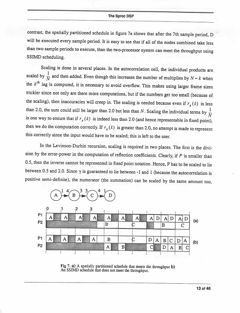
one on which frequently firing cells get partitioned. Figure 7 illustrates a case where we have 2
processors and where the overall execution time of the graph is longer than 2 sample intervals. B
and Ccan represent the autocorrelation and Levinson-Durbin cells for example. Hence, the worst
case execution (in the Star context) occurs every fourth sample period. During the other sample
periods, B and C execute some synchronization code; the duration is much shorter. As can be
seen, D (which can represent a D/A) won't be executed during sample periods 3,4,5, and 6. In
x(n) x(n+l) x(n+2) x(n+3) x(n+4) x(n+M+l)
count=0 1At this pointwe have i
enough data. 1
Compute
MO)Compute
lCompute
MDCompute
M+l
ICompute
rx(M)
ComputeaM(0
Copy contentsinto an internalarray
Initializelpc coeffs array
Fig 6. Computation procedure for LPC coefficients. In each sample intervalone pass of theLevmsoniteration takes place.
12 of 46
»oooooo60ociftftnciBaacaeoetiaa<oaoa&o
The Sproc DSP
contrast, the spatially partitioned schedule in figure 7a shows that after the 7th sample period, Dwill be executed every sample period. It is easy to see that if all of the nodes combined take lessthan two sample periods to execute, than the two-processor system can meet the throughput usingSSIMD scheduling.
Scaling is done in several places. In the autocorrelation cell, the individual products arescaled by - and then added. Even though this increases the number of multiplies by N-k whenthe k1 lag is computed, it is necessary to avoid overflow. This makes using larger frame sizestrickier since not only are there more computations, but if the numbers get too small (because ofthe scaling), then inaccuracies will creep in. The scaling is needed because even if r {k) is lessthan 2.0, the sum could still be larger than 2.0 but less than N. Scaling the individual terms by -is one way to ensure that if rx (k) is indeed less than 2.0 (and hence representable in fixed point),then we do the computation correctly. If rx (k) is greater than 2.0, no attempt is made to representthis correctly since the input would have to be scaled; this is left to theuser.
In the Levinson-Durbin recursion, scaling is required in two places. The first is the division by the error-power in the computation of reflection coefficients. Clearly, ifP is smaller than0.5, then the inverse cannot be represented in fixed point notation. Hence, Phas to be scaled to Hebetween 0.5 and 2.0. Since yis guaranteed to he between -1 and 1(because the autocorrelation ispositive semi-definite), the numerator (the summation) can be scaled by the same amount too,
&A^p7pS
Fig 7. a) Aspatially partitioned schedule that meets the throughput b)AnSSIMD schedule that does notmeet the throughput.
(a)
(b)
13 of 46

•BMMMMMMMI
The Sproc DSP
without fearing overflow. The second scaling has to be done for the filter coefficients themselves.
Equation 1 shows that the initial value, a0 (0), determines the value of the coefficients for all
orders greater than 1. To seehow starting therecursion with a0(0) = b affects thecomputation,
where b is some number less than 1.0, denote by Y the values of the reflection coefficients, and
by ak the filter coefficients generated by the algorithm when a0'(0) = ^ We get that
YL' = -brx(l)/rx{0). So yx = y{/b. If we use yx in equation 1, we get 0/(0) = b and
*i'(l) = Yj^u'W = Yi^- Therefore, ax'(i) = ba1(i),i = 0,1 . Now we can see that
y2' = byl when a<{ (i), i = 0,1 is used in equation 2. Sowe can always compute y^ from yk
by y^ = yk/b and use y^ in equation 1 to compute ak'(m) where ak(m) = bak(m). What
this shows is that starting the recursion with a0'(0) = b results in the filter coefficients being
scaled by b. Therefore, we would like toknow what b should betoensure that ak (m) is always
less than 1.0 in magnitude. It turns out that choosing b = 0.25 works well in practice, but an
exact bound can be derived, as is done in section 3.5.2.1.
The cells were tested by constructing a simple speech coder. The Levinson-Durbin cell is
used to generate the prediction error filter coefficients, which is used by anFIR filter to generate
the error sequence. The error sequence, which should hopefully have much less energy than the
speech signal if the prediction is good, is coded using a 3-bit adaptive quantizer. The speech sig
nal is reconstructed by inverse filtering which can be achieved by having an FIR filter in a feed
backloop, using the same coefficients generated by theLevinson-Durbin recursion (fig. 8).
Fig 8. A simpleLPCcoder
14 of 46
1 —Ii
FIR w
/\
DA

The Sproc DSP
3.5.2.1 An upper bound for a^O)
By upper bound we mean the value b such that
\a0(0)\£b=*\ai(m)\£1.0 V/,/n = 0,1, ...,M (EQ5)
Theorem 1: Equation 5is satisfied if b=1/ (f ** 1).
Proof:
First we need a few facts and lemmas.
Lemma 1:
*-i
a/(m)|̂ £(|a.^(m-y)| +|a/.,(/-m-y)|)^-1J V* =1 /Proof of lemma 1:
(EQ6)
Theproofis byinduction on k. We have from equation 1 that
\ai(m)\£\ai_1(m)\+\ai_l(i-m)\
Letting k = 1 inequation 6,we see that the base case holds. Now assume it holds for k-l. From
equation 1, we have that
|a/-it(w-;)|^K_^1(m-y)| +|aJ..it.1(/-/:-m+7)|, (EQ7)
and that
\oi.k(i-m-j)\^\ai_k_l(i-m-j)\+\ai_k_1(m+j-k)\ (EQ8)
15 of 46

The Sproc DSP
Now, 0 £ j'<, k - 1 => A: £ k -j £ 1. If we substitute equations 7 and 8 in equation 6, we will get
four terms in the summation. Consider the term |a,._kmm j (/ - m- (k-j)) |. The summation
r
|«/-t-i('-'«-«|^1J+-» +|fl/.*-i('-«-l)|l{.lJ-
*-l
*-l
8 by
V |ai-*-1 (' ~m~ 0* +1)) 11 7 J*Similarly, we can replace m- (k -j) in equation7-0
m - (jf + 1). If we substitute equations 7 and 8 into equation6 with these index changes, we get
two summations, each of the form
*-i
Y (fl(w-/)+fl(m-7--l))l*-lyrt v J ;
(EQ9)
where the subscript / - k - 1 has been omitted for clarity. Equation 9 can be expanded as follows:
(a(m) +a(m-l)) Jt-1
k o ;+ (a(m-l)+a(m-2))r~1 + ...
...+ (a(m-k+l) +a(m-k))( \
k--1
U-•l)
aOiO^J+flOii-lH^-1 'v)>+•••+«<»•-*> (j:£
V a(m -y) I.J where we have used fact 2.
Applying this to equation 6, we see that it is satisfied for k if it's satisfied for k - 1. QED
Lemma 2: \at (m) \£\a0 (0)
Proof of lemma 2:
16 of 46
MKM/2J \/0£i,m£M

attra-*xo.>x>oooooceooc<w«»o^^
Code Generation in Ptolemy
Letting k = i in equation 6, we get
«/(m)|££ (\ao(™-J)\+\a0(i-m-j)\)[i-1); _ n \ J sy-o
since the summation for A' - 1is less than the summation for k. Suppose that 1£772 £/- 1. Then,l£i-m£/-l. Since a0(/) = 0, V/*0, we get
\ai(m)\<. '-1 + M l^o(0)1 = fln(0)m;iuo (EQ10)
where we have used Fact 1. For the case m=/, we have that |q(/) | <; |*0 (0) | from equation 1.For m>i, at (m) = 0 and for m= 0, a. (0) = g0 (0). We have
/ \ / \
Therefore, the lemma follows. QED
1
\jn)M
M/2)
This implies that if \aQ(0) |£1/ I^J, then |tf|(m)| <; 1.0, V0<; i, m̂M. Hence thetheorem is proved. QED.
For M= 12, areasonable value, we should make aQ (0) e 0.001 to ensure that the computations never overflow. Since bwill typically be small enough that b~l is greater than 2.0, forefficiency, we should set aQ (0) to be the largest power of two that is less than the calculatedbound. This will allow the reflection coefficients to be scaled using shifts instead of multiplies.Thecell was implemented with these considerations in mind.
4 Code Generation in Ptolemy
Adomain in Ptolemy consists of Stars, Targets, and Schedulers. The Wormhole interfaceis optional and is used only if the domain being designed is going to be used with other domains
in a single universe. The algorithm to be implemented is represented as a hierarchical dataflow
graph. The graph is built hierarchically out ofstandard library Stars or user-defined Stars that canbe linked in dynamically.
17 of 46

Code Generation in Ptolemy
Functional stars that generate the actualcode, e.g. SprocFir.
Ptolemykernel(not a specificdomain)
SDFDomain
CGDomain
Fig 9. Derivationhierarchyfor SprocStar. SprocStaris derivedfrom AsmStar in the CG domain
4.1 Stars
Currently, there are two types of stars in Ptolemy, code-generation stars and simulation
stars. Figure 9 illustrates the derivation hierarchy for stars in the Sproc domain. As can be seen,
the CG domain (which is the baseclass for all code-generation domains) is derived from the SDF
domain and the SDF domain is derived from the kernel as is every domain in Ptolemy. Note that
this derivation hierarchy can change in the future when code-generation will be extended to more
general models of computation like dynamic dataflow and boolean dataflow [Buc92]. Derivation
here refers to the object-oriented inheritance concept in which one class can be derived from
18 of 46

MeMMomcMeeeaMMi
Code Generation in Ptolemy
another class. The derived class will be asuperset of its parent class meaning that methods and
certain types ofdata members from the parent class are available to the derived class. In addition,the derived class can have new data members, new methods, and re-definition of methods from
the parent class if those methods are virtual methods. In SprocStar some simple functions havebeen redefined; for example, the function that prints out state values isredefined todo it inhexadecimal.
Stars are relatively easy to write because there is apreprocessor language called ptlangthat translates astar description to C++. The star description is given in a"boilerplate" format bydefining states, ports, and various methods, ptlang then parses the file and generates the appropriate cc and h files that the compiler can understand. An example ofthis code for the star SprocGainis given in figure 11. The go () method inthe star is called when the universe in run. In simula
tion stars, this method will perform the actual function of the star, whereas in code-generationstars, this method will call the addCode (CodeBlock&) method which will add the code con
tained in codeblocks to acode stream inthe target. There are two other functions that are used: the
setup () method and the initCode () method. The setup () method is called before go ()and is responsible for setting up information that will be needed by the scheduler and memoryallocator, such as the size ofarrays, the number ofsamples read from aparticular port etc. Forexample, in figure 12 the setup () method resizes the coefficients vector and sets aparameterfor the input port indicating that Dsamples will be read, where Dis the downsampling factor forthe star. The initCode () method is called before the go () method and is used to generatecode that appears before the main loop; code to initialize portholes for example (fig. 10).
The assembly language code is contained in codeblocks. A complete star description isgiven in figure 11 for the star SprocGain. Notice that the codeblock has constructs of the form
$addr or $val. These are called macros. The addCode method will substitute the appropriate values when the codeblock is parsed. The most commonly used macros in Sproc stars are given intable 1.
Calling the noInternalState () methodin the constructor tells the scheduler that the
star has nodependence onpast computations. This is toallow the scheduler the option of schedul-
19 of 46

wttttMimbtctut
Code Generation in Ptolemy
codeblock (initfill) {// initiallization code for $starnaine()Ida #$val(fill)ldb #$addr(output)ldd #1ldl #$size(output)-1$label(lpl):sta [B+L]djne $label(lpl)}initCode { if ((factor > l)&(fill != 0.0) ) addCode(initfill); }
Fig 10.The InitCodemethodfrom SprocUpsample initializes the outputport to a value.
ing multiple invocations of this star simultaneously on different processors, thereby extracting
more parallelism (see section 4.4.2). The execTime () method is used by the scheduler to find
out how much time this star takes to execute; the star writer must provide this.
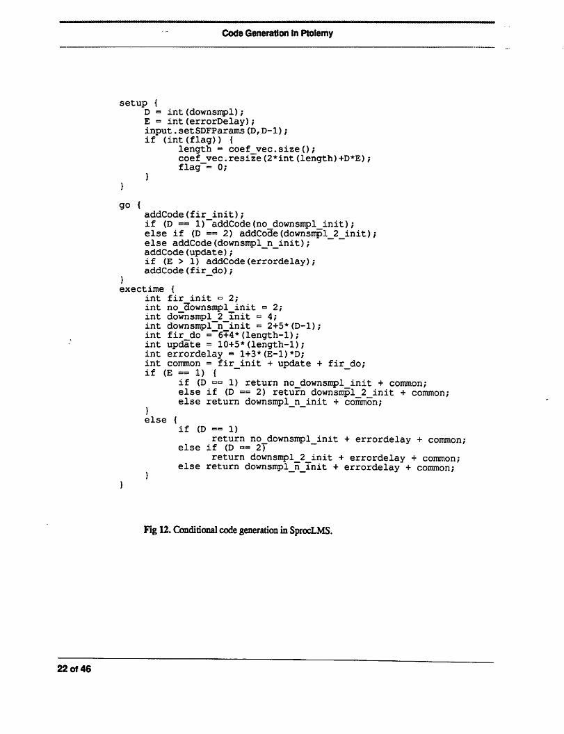
One of the advantages of star-writing in Ptolemy is thepossibilityof conditionalcode gen
eration. A good example of this is the go () method from the SprocLMS star (figure 12) which
implements an adaptive filter using the LMS algorithm. There are two parameters for the star: the
down-sampling factor and the number of delays on the error input (since the error is computed
from the output at some stage, there is a feedback loop implying an error delay of at least 1.)
There arevarious optimizations possible in thecode forparticular combinations ofparticular val
ues of these parameters, and this results in the code being stitched together appropriately by the
go () method. Also, note how the execution time is calculated in the execTime method for the
various combinations of the input parameters. The execution times for each of the code sections
are provided by the programmer.
Table 1. Commonly used macros in SprocStars
Macro Use
$addr(memory_name) Substitutememoryaddress.
$addr(pormame, offset) Substitutememoryaddresswith added offset.
$val(state_name) Substitute numerical value of the state.
SstamameO Substitute the name of the star.
$labeI(foo) Create unique label from "foo" by adding aunique identifier.
20 of 46

Code Generation in Ptolemy
defstar {name { Gain }domain { Sproc }desc {
The output is set to the input multiplied by a gain term.The gain must be in [-1,1].
}version { @(#)SprocGain.pll.512/8/92 }author { P. Murthy }copyright {
Copyright (c) 1990, 1991, 1992 The Regents of the University of California.
}location { Sproc stars library }explanation {}execTime {
return 5;}input {
name {input}type {FIX}
}output {
name {output}type {FIX}
}constructor {
noInternalState();}defstate {
name {gain}type {FIX}default {1.0}attributes {A_RAM}desc {Gain value}
}codeblock (std) {
//_$starname()_begin:ldx $addr(input)mpy $addr(gain)nop
nop
stmh $addr(output)}go {
addCode(std);}
}
Fig 11. Code for star SprocGain
21 of 46
22 of 46
nemmeMMMMa
Code Generation In Ptolemy
setup {D = int(downsmpl);E = int(errorDelay);input.setSDFParams(D, D-l);if (int(flag)) {
length = coef_vec.size();coef_vec.resize(2*int(length)+D*E);flag = 0;
}}
go {addCode(fir_init);if (D == 1) addCode(no_downsmpl_init);else if (D == 2) addCode(downsmpl_2_init);else addCode(downsmpl_n_init);addCode(update);if (E > 1) addCode(errordelay);addCode(fir do);
}exectime {
int fir init =2;int no_3ownsmpl_init =2;int downsmpl_2_init = 4;int downsmpl_n_init «= 2+5*(D-l);int fir_do = 6+4*(length-1);int update = 10+5*(length-1);int errordelay = 1+3*(E-1)*D;int common = fir_init + update + fir do;if (E == 1) {
if (D == 1) return no_downsmpl_init + common;else if (D == 2) return downsmpl_2_init + common;else return downsmpl_n_init + common;
}else {
if (D == 1)
return no_downsmpl_init + errordelay + common;else if (D == 2)
return downsmpl_2_init + errordelay + common;else return downsmpl_n_init + errordelay + common;
Fig12. Conditional codegeneration in SprocLMS.

Code Generation in Ptolemy
4.2 Targets
A target in Ptolemy defines those features ofan architecture that are pertinent to code generation. It will specify how the generated code will be collected, specify and allocate resourcessuch as memory, and define the code necessary for proper initialization ofthe platform. It mayalso specify how to compile and run the code if the platform being targeted is directly accessiblefrom the platform that Ptolemy runs on. There are two types oftargets in Ptolemy, multiprocessortargets and single processor targets. The difference is that amultiprocessor target will contain several child targets that are single processor targets. This allows code re-use in that once asingleprocessor target has been defined for aparticular processor, any architecture containing multiplesuch processors need only define a parent multi-target, making use of the imgle-targets thatalready exist. An example ofthis is the OMA architecture [Bie90] where the OMATarget is builtfrom existing Motorola 96000 targets [Sri93]. The derivation hierarchy for targets is shown in figure 13.
CGTarget is the baseclass for all code generation targets including multiprocessor targets.The CGMultiTarget represents atarget for ageneric, fully connected architecture. No assumption
Fig 13. Derivationhierarchy for targets
23 of 46

Code Generation in Ptolemy
is made about the memory resources available. The main job of this target is to define various
parameters for the multiprocessor schedulers assuming the fully connected topology (communica
tion costs, schedules for use of communication facilities etc.) Fully connected means that every
processor in the network can communicate with every other processor in the network, and that the
communication time is not a function of a particular communicating processor pair. This model is
appropriate for the Sproc since the shared memory allows each processor to communicate with
any other processor. The shared memory also implies that the communication time is not depen
dent on the processors. There is another target called CGSharedBus which assumes that commu
nication among processors occurs through a shared bus and hence sets up the schedulers so that
bus contention cost is taken into account.These two generic targets fit most parallelDSP architec
tures quite well. In addition to having methods for defining various parameters for schedulers,
CGMultiTarget has a method for creating and initializing child targets, which are derived from
AsmTarget, and a method for choosing and initializing the multiprocessor scheduler based on the
user's selection. The general method by which a particular architecture is targeted is then to
derive a parent target from CGMultiTarget or CGSharedBus. The parent target is responsible for
any shared resources andthe child targets are responsible for private resources local to the proces
sor.
4.3 Schedulers
There are two multiprocessor schedulers of interest to the Sprocdomain. One is Hu's level
based list scheduling [Hu61] and the other is Gil Sin's declustering scheduler [Sih91]. There is
also Gil Sin's dynamic level scheduler, but this assumes that processors have the ability to do
computations in parallel with communication. Since the Sproc does nothave this ability, it is not
used. The parent target contains parameters that allow the user to choose between either of these
schedulers. Since the schedulers behave differently for all butthe most trivial graphs, this flexibil
ity is useful for selecting the best schedule. In addition, the user can manually schedule the graph
by setting a state in each star that tells the scheduler the processor on which the star should be
scheduled. The schedulers are responsible for partitioning the graph across the different proces
sors, taking interprocessor communication into account. Once the graph has been thus partitioned,
24 of 46

Code Generation In Ptolemy
sub-graphs are created for each processor and an order for firing the blocks is determined. Since
each uniprocessor target hasauniprocessor scheduler object, which in turn has adata structure for
storing the schedule, the scheduled sub-graphs are handed down to the uniprocessor schedulers'
schedule data structure. This allows the child target to execute its sub-graph without knowingwhere it came from, thus preserving the modularity of the target hierarchy. The parent target,
however, has to ensure that the uniprocessor scheduler in each child target does not get invokedsince the schedule will be provided by themultiprocessor scheduler.
4.4 Interprocessor communication
4.4.1 Send/Receive
Interprocessor communication (IPC) is implemented using the send-receive model. In this
model, send stars are inserted whenever one processor wishes to communicate data to another
processor. The receiving processor will have areceive star that will receive the data. No assump
tion is made about how these stars will be implemented; that is part ofthe target/domain design.The scheduler is merely told the cost involved (i.e., the execution times ofthe send and receive).
Once the sub-graphs are created, the scheduler inserts these communication stars at the appropriate places and schedules them along with the other stars in the sub-graph. For an example, see figure 14. A side benefit of this approach is that no sub-graph will have unterminated connections.
This is important because each child target behaves exactly as if its sub-galaxy were the whole
universe and unconnected terminals are not allowed inany graph the user might create.
4.4.2 Spread/Collect
In multirate applications, it is often possible to extract more concurrency out of the graph
byexecuting multiple invocations ofablock simultaneously on different processors. This is pos
sible with actors that do not contain state variables; the noInternalState() directive mentioned in
section 4.1 informs the scheduler of this. Figure 15 shows a simple example of this.
Since Bl (the first invocation of B) requires a sample from A2 and A2 is scheduled on
processor P2, a way is needed of collectingthe three samples required for Bl (2 from Al, 1 from
A2). The reason we have to collect these samples is that the original node B only has one input
25 of 46

The Sproc domain
&O-® p,I
Rev * CA
B SndB
A
Rev
(a) (b)
B Snd
(c) (d)
Fig 14. Send/Receive Model, a) A graph, b) A two processor schedulewith IPC stars, c) sub-graph for PI, d) sub-graph for P2
arc. The code inside will make reference only to this input arc. In the APEG graph, however, each
invocation of B has three arcs. We cannot allocate memory separately for these arcs because they
won't be referenced in the codeblocks. Hence, a "Collect" star is inserted as shown in figure 15.
This star tells the memory allocator that the three output locations on the Collect stars output arc
should be aliased to the two outputs on A and one to the receive star output. Similarly, of the four
samples produced by A2 and A3, one is sent to PI while the rest are used by B2. This behavior
can be implemented via a "Spread" star. The subgalaxies created by the scheduler are shown in
fig.15d.15e.
The Sproc domain
The Sproc domain consists ofa set oftargets, an experimental scheduler, and a library of
stars.
26 of 46

MMMMMMMMMMI
The Sproc domain
GP0(a)
©t^^(b)
P1
" 1 R Bl
P2 A2 S A3 B2
02 2
Jg
Rev^
1 1
3 3
(c)
B
1 1
•o
Snd
«
Sa 3 3/^X
CO / - ^—w
^
(d) (e)
Fig 15. Spread/Collect a) Multirate graph, b) Acyclic precedenceexpanded graph (APEG), c) Schedule, d) Sub-galaxy for PI, e) Sub-galaxy for P2
5.1 SprocTarget
This is the main parent target object derived from CGMultiTarget as shown in figure 13. It
controls the creation and pairing ofIPC stars, itis responsible for initializing the child targets, anditcoordinates the memory allocation process with the child targets. Figure 16 shows the sequenceof function calls that take place. Only the important calls are shown. Some of the calls have a
name beside themin brackets; this name indicates theclass from which thecalled function will be
27 of 46

WMMMOMMWMttl
The Sproc domain
executed because of the virtual mechanism. The basic function troika is setup (), run (), and
wrapup () (recall that these are the main functions in stars as well). At what level in the deriva
tion tree one of these gets called depends on the function. For example, SprocTarget has
setup () and wrapup () but no run () because the definition in CGMultiTarget suffices. The
scheduler object is chosen during setup () in the Target as shown. The schedule is computed
during setup () and the code generation occurs during run (). Memory allocation is done by
the allocateMemory function and functions such as beginlteration () and endlter-
ation () are used for generating looping code. In SprocTarget the number of iterations is cur
rently ignored but in general these methods should generate code takingthatnumberinto account
because loop schedulers call the same functions to generate the looping code within a schedule.
Since loop schedulers are not used in parallel code-generation, this is not an issue in the Sproc
domain.
28 of 46

The Sproc domain
SprocTarget:: setup()create the memory objectCGMultiTarget:: setup()
createChildO [SprocTarget] //create child targetschooseSchedulerOTarget:: setupO
scheduler:: setupO [SDFScheduler]computeScheduleO [ParScheduler] //main schedule
createSendOcreateReceive()pairSendReceiveO [SprocTarget] //pair eachsnd w/rcv
headerCode()CGMultiTarget:: mnO
CGTarget:: run()generateCode() [CGMultiTarget]
scheduler()->compileRunO [P arSchedu1er]UniProcessor(i):: prepareCodeGenO
convertScheduleO // copy par.sched to targets'simRunScheduleO // trace schedule for rightbuffersizes
mtarget->prepareCodeGen [SprocTarget]build a galaxy from several sub-galaxiesinstantiateO
resizeBuffer() // for I/O stars based on makespanfirstChild->setup() [SprocGspTarget]
allocateMemory() [AsmTarget]codeGenInit() [AsmTarget]
doInitializationO [SprocGspTarget]writeInt,Fix etc
UniProcessor(i):: generateCode()child(i)->generateCode() [SprocGspTarget]
headerCode()initCodeO // fire stars initcode methodsmainLoopCodeO [CGTarget]
beginIteration() [SprocGspTarget]scheduler()->compileRun [SDFScheduler]
fire go() methods in starsendIteration() [SprocGspTarget]
Target: :wrapup()wrapup each star
addProcessorCodeO // append code to stream in parentSprocTarget:: wrapupO
frameCodeO // generate any framing code required for programprintDataRam [SprocMemory] //generate memory initialization mapDump code to files
Fig16.Function call sequence for code-generation
29 of 46
•MMMMMMMMi MOmmMMMttMMMMMttMCaaMMOMMMMMMI
The Sproc domain
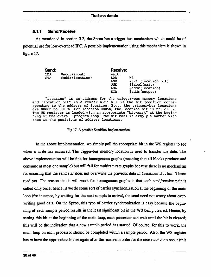
5.1.1 Send/Receive
As mentioned in section 3.2, the Sproc has a trigger-bus mechanism which could be of
potential use for low-overhead IPC. A possible implementation using this mechanismis shown in
figure 17.
Send: Receive:LDA $addr(input) wait:
STA $addr(location) LDA WS
AND #$val(location bit)JNE $label(wait)LDA $addr(location)STA $addr(output)
"Location" is an address for the trigger-bus memory locationsand "location bit" is a number with a 1 is the bit position corresponding to the address of location. E.g., the trigger-bus locationsare 0800h to 0817h. For location 0805h, the location_bit is 2A5 or 32.The WS register is loaded with an appropriate "bit-mask" at the beginning of the overall program loop. The bit-mask is simply a number withones is the positions of address locations.
Fig 17. A possibleSend/Rev implementation
In the above implementation, we simply poll the appropriate bit in the WS register to see
when a write has occurred. The trigger-bus memory location is used to transfer the data. The
above implementation will be fine for homogenous graphs (meaning that all blocks produce and
consume at most one sample) but will fail for multirate rate graphs because there is no mechanism
for ensuring that the send star does not overwrite the previous data in location if it hasn't been
read yet. The reason that it will work for homogenous graphs is that each send/receive pair is
called only once; hence, if we do some sort of barrier synchronizationat the beginning of the main
loop (for instance, by waiting for the next sample to arrive), the send need not worry about over
writing good data. On the Sproc, this type of barrier synchronization is easy because the begin
ning of each sample period results in the least significant bit in the WS being cleared. Hence, by
setting this bit at the beginning of the main loop, each processor can wait until the bit is cleared;
this will be the indication that a new sample period has started. Of course, for this to work, the
main loop on each processor should be completed within a sample period. Also, the WS register
has to have the appropriatebit set againafter the receive in order for the next receive to occur (this
30 of 46

——————— rrTtniriinnnnniim mmiumuiinii
The Sproc domain
is assuming that a particular send/receive pair is invoked more than once in a schedule period).
Again, for homogenous graphs, this won't be a problem since with barrier synchronization, we
can assume that all send/receive pairs have executed and reload thebit maskintotheWS register
atthe beginning of themain iteration. It turns out that setting abitin the WS register and ensuring
that the send star does not overwrite previous data requires more overhead than the usual sema
phore approach. In particular, a single instruction for setting a bit in the WS register does not
exist; so three instructions would berequired to set abit. In addition tothese disadvantages, there
are only 18 trigger bus locations which puts a limit on the number of IPC stars, an undesirable
prospect.
Therefore the approach used is a semaphore mechanism. In this scheme, the Send star will
write the datum onits input to the output of the Receive star if the semaphore location contains a
one. Otherwise, it waits until the condition is met. After the write to the Receive's output, the
semaphore location is reset to a zero. The Receive star merely examines the semaphore location
and if it is one (meaning that a new datum has not arrived), it waits until the location has a zero.
The code for doing this is shown in figure 18.
Send: Receive:idl #0 Ida $addr(pollAddr)ldx $addr(input) jne $label(wait)$label(wait): std $addr(pollAddr)Ida $ref(pollAddr)jeq $label(wait)stl $ref(pollAddr)stx $ref(output)
Fig 18. Send/Rev implementation
It is worth noting that a rather roundabout methodis used to enable the Send star to write
directly to the output on the Receive star. Recall that aSend star does not have an output port and
a Receive star does not have an input port because one is a sink while the otheris a source in the
sub-galaxy in which each exists. However, the macro function that actually computes the address
of a location canbe re-defined in the Send star because this is avirtual function in CGStar. The re
defined method simply looks up the Receive star's output location even though the codeblock in
31 of 46

•MMMMMeeomttMW
The Sproc domain
the Send starrefers to a non-existent "output" port.The parent target ensures that each Send star
has a pointer to the Receive star that it has been paired with. The same technique is used for the
semaphore location as well, since this has to be a state in either the Receive or the Send.
The overall executiontime is 9 cycles,with the Send star requiring 6 cycles. An advantage
of this scheme is that the semaphore location canbe allocated just like any othermemory location.
It does not require a special region of the memorylike the trigger-bus region. Even though it is a
waste of memory to use 24-bit locations for storing single bits, a single location or register for
multiplebits cannot be used withoutinstructions for bit setting andclearing.
5.1.2 Memory Allocation
Since the Sproc has a shared-memory architecture, only onememory object is required in
the Target definition. The parent target creates this object during setup () and a pointer to the
object is passed to each child targetwhen the child target is createdso that each child has access to
the same object. The memory allocator functions are all called by AsmTarget (the baseclass for
the child targets). The order in which this occurs is as follows: requests for all memory are posted
first. For the child this means all the states andports in its subgalaxy. Then the performAllo
cation () method is called to process all the requests. The request-allocation sequence, how
ever, canonly happen once foreach memory object because of the way the allocation routines are
written. So for a shared memory object, justhaving each child go about memory allocation on its
turn fails because the request-allocate sequence will occur once for each child and we want it to
occur only once. Therefore, the parent intervenes with a method called prepareCodeGen (),
which is called before the generateCode () method (the generateCode () method is the
usual way of passing control to the child targets for memory allocation and code generation). In
prepareCodeGen (), one galaxy is created outof the subgalaxies for each of the processors.
This galaxy is then re-instantiated because the original instantiation is lost when the sub-galaxies
were created in the first place. After the re-instantiation, the memory allocation methods are
called through one of the child targets. Now when the generateCode () method is called, the
child targets simply fire the stars in their subgalaxies and add the generated code directly to a
stream in the parent target. The wrapup method in the parent then writes the contents of the
32 of 46

The Sproc domain
stream to a user-specified file. The initialization code for the memory is also generated duringwrapup () via a method in the SprocMemory class.
Normally the initialization is done in AsmTarget via "org" like statements. The Sproccompiler, however, does not have such astatement, and the only method for initializing the mem
ory is by statements such as variable fixed foo = 1.5. Moreover, these statements have to
occur in order ofthe memory map since there is no way (without run-time code) to initialize specific memory locations. The initialization method in AsmTarget does not initialize port locations,something that is required for the Sproc. Hence, the dolnitialization () method is rede
fined in the child targets to permit port initialization, dolnitialization () calls virtual
methods such as writelntO (for writing integers), writeFix(), and writePort().
These would normally generate compiler statements such as dc l. 5(on the Motorola 56000) but
here these methods write the values to global arrays maintained inthe parent target. This is done
so that the memory initialization can be done in order of memory rather than the order of stars.
Three arrays are maintained: one for the name ofthe state or port, one for the type, and one for the
value. These arrays are then read by the method printDataRam () in the SprocMemory classduring the wrapup () in the parent target and the "variable" declarations are generated andwritten to another file. Having the names in the initialization serves another useful purpose,namely to allow efficient debugging and change ofstate values while the program is nmning onthe chip through the SDI interface on the PC.
5.1.3 I/O
Programmable buffering is used for the input/output stars. One weakness ofthe SDF paradigm is that since there is no concept oftime, it is assumed that source stars can be fired at anytime. This is obviously not true in the case ofA/D stars where the star is actually synchronouswith an external sample rate. Therefore the schedulers, which are based on SDF, will schedule
input/output stars without taking the sample rate into account. When aschedule period containsmultiple invocations ofan input star, itis crucial that some method be used to ensure that samplesare not lost. In the Motorola 56000 domain, interrupts are used if there are multiple invocations.
The Sproc has programmable buffers where the size can be set before-hand; this loosens the con-
33 of 46

MCCMMMMMMMMI
The Sproc domain
straintof an input block having to fire every sample periodto aninput block having to fire N times
in N sample periods (if the schedule requires N firings of this input block). This eliminates the
need for interrupts and the loss in processingtime that results. The buffer size is set automatically
by the target by calculating the number of sample periods overwhich the schedulewill run.
5.1.3.1 A possibility for future work
Even though programmable buffering is a better solution than interrupts, the best solution
would be for the scheduler to take into account periodicitiesof certain stars. This could then result
in schedules where the I/O stars are executed in each sample period, eliminating the need for any
buffering at all.This is generally a difficult thing to do becausenot only does the I/O star have to
fire every sample periodbut all starsthatwork at the sameratemust also fire every sample period.
This is especially difficult since all such stars may not be on the same processor and some may
even have execution times greater than a sample period. If I/O stars can be scheduled on different
processors for different invocations, then meeting the no-buffering goal might be possible. But
given that the number of different combinations of schedules for schedulingN invocations of an1/
O star on P processors is PN, the problem may not have a polynomial time solution in general.
Figure 19 shows a simple example of an efficientschedule if source stars are scheduled on differ
ent processors.
5.2 Other Targets
Two other targets have been written. One target generates code in the form of high level
function calls. In other words, instead of in-line assembly code in the program, a statement con
taining the name of the block, its states, and its input and output ports is generated. The Sproc
compiler then generates code for these functions from the Sproc library of assembly language
cells. Therefore this requires there to be an exact match between Ptolemy stars and cells in the
Sproc library. This requirement is not very attractive because as discussed before, stars in Ptolemy
aremore general in terms of theirmultiratecapability andtheirability to do conditionalcode gen
eration.
34 of 46

The Sproc domain
Al Bl A3 B2
illilf^l^i'!- A2 CI
a I ♦ i
Fig 19. Example of sourcestars fired on different processorsfor alternate samples.
The other target is a test for an experimental scheduler understudy. This targetjust sets up
the scheduler object and does not do anything else. It illustrates the ease with which new targets
and schedulers can be written based on existing code.
5.3 Some examples
Some applications developed include the Karplus-Strong algorithm for simulating
plucked string sounds (this is done in a way that turns the PCinto a mini keyboard), reverberation
of an audio signal, a three band QMF filter bank, and ADPCM encoding and decoding of speech
using LMS filters. Three of these are described below.
5.3.1 Plucked strings
The Karplus-Strong algorithm is a simple, elegant way of simulating plucked string instru
ments like guitars and harps [Moo90]. A plucked string can be modeled as a digital delay line
with a low- pass filter in a feedback loop. The delay line is initially filled with random samples;
this signal represents an excitation signal that is rich in harmonics. As the signal circulates in the
feedback loop, the low pass filter attenuates the higher frequencies. This results in a signal that
35 of 46

The Sproc domain
sounds like aplucked string instrument when played through aspeaker. The length of the delay
line, which is equivalent to the length of the string, determines the pitch of the resulting sound.
While the delay line can only contain integer values, it is possible to get fractional delays by
including anall-pass filter in series with thedelay. This wouldthenallow the model to be tunedto
desired frequencies quite precisely.
Figure 20 shows seven of these modules connected to aD/Aconverter. The pulse star in
each module generates arectangular pulse that has aduration equal to the length of the delay line
for that module. The values of the delays in each module are chosen to roughly approximate an
incomplete scale. Through the access port on the Sproc board, the user can set a flag in the prise
star. The pulse star generates apulse only if this flag is set. After generating the pulse, the star will
reset the flag and generate zeros. Therefore, by tying commands that set this flag to particular keys
on the IBM PC keyboard, one gets the effect ofamusical keyboard bypressing different keys that
trigger one or more ofthe modules. Note that even though the behavior ofthe pulse star appears to
be asynchronous, it isnot really being used in that manner since it is fired on every iteration. The
star decides, based on its flag, whether to generate apulse or not, rather than generating one peri
odically. This application is partitioned onto all four processors and the makespan is exactly 200cycles.
5.3.2 QMF Filter bank
Figure 21 shows athree-band quadrature mirror filter (QMF) bank. The principle behind
QMF filter banks is as follows. Signals ofpractical interest, for example, music signals or speech
signals, do not contain equal amounts ofenergy in all parts ofthe spectrum. Hence, if itwere pos
sible to separate the signal into components for different frequency regions, each frequencyregion could be coded separately based on the amount ofenergy it has inthat part of the spectrum.
One way of obtaining these components is to recursively divide the spectrum by half at each
stage. In other words, a high-pass and a low-pass component is created by filtering and then one
of these is further subdivided until one has enough bands. For speech signals, where the energy is
typically in the low-pass region, it's the low-pass component that is subdivided at each stage.
Note that by dividing the spectrum by two, we obtain two band-limited signals that can be deci-
36 of 46

MMMMMW«M«MMUMI
H/
L
L
L
L
L
L
L
The Sproc domain
<&—-€>—er~^*', ,*..»
U&
e—€>•€>—~&T^ tfC30
m
g>—®—d> —(-<
'. .«. I
m
^g>—^ (g^HQT^I, ,4, ,)
m
-€>—€>-h2C^m
Hg>—€>—^k-hST^m
e—€>—er
m
Fig 20. The multi-string bank. Each bank generates aplucked string sound atagiven frequency using theKarplus-Strong algorithm
•<S>—»/ft
€^
37 of 46

The Sproc domain
£> ^i
fi/D ^ d/a
Fig 21. A 3-band QMF filterbank. The left side consistsof the analysis filters and the right side the synthesis filters
mated by two. So even though we have two signals, each is transmitted at half the original rate.
The reduction in the transmission rate comes aboutbecause fewer bits will typically be required
to code one of the components. The choice of the analysis filters is very important since the recon
structed signal usually differs from the original signal due to aliasing, amplitude distortion, and
phase distortion. However, the filters can be designed in such a way that some (or all) of these dis
tortions are eliminated. See [Vai93] for a good introduction to the theory and design of filter
banks.
Figure 21 contains 2 stages: the low-pass component of the first stage is subdivided again
into two bands. We get three bands overall, and in the example, we can vary the gain in each of
the paths to get the effect of an audio equalizer. The FIR filters that implement the high-pass and
low-pass filters (figure 22) also do the decimation (interpolation) in the analysis (synthesis)
stages. This is because the implementation of the filter is much more efficient if the decimation is
taken into account; samples that are thrown away, as is the case during decimation, are not com
puted, and multiplies with zeros, as is the case during interpolation, do not occur. More stages are
not used because each additional stage causes the code space to more than double because of the
decimation/interpolation. Given that there are only Ik words of program memory available, any
thingmorethan 2 stages is currently not feasible. However, if loopscheduling techniques [Bha93]
are extendedto the multiprocessor case (possible future work), thenthe codespace problem might
be mitigated.
A small fraction of the generated code for this universeis given in the appendix (all of it
isn't given since many trees would have suffered).The filter bank runs at a sample rate of 9.7kHz.
38 of 46

The Sproc domain
<
I + I
Fig 22. The analysis block expanded; the top is alow-pass FIR andthe bottom ahigh-pass FIR
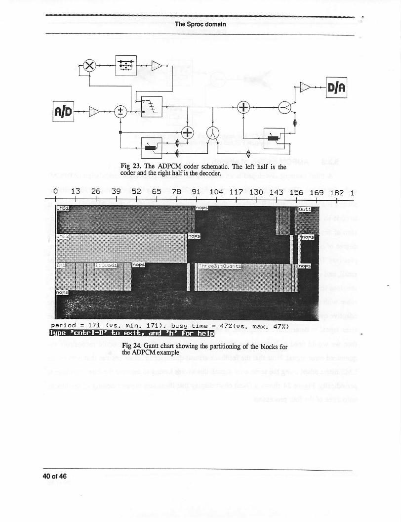
5.3.3 ADPCM coding of speech
A third example developed is an adaptive differential pulse code modulation (ADPCM)
coder for speech.The coder/decoder shownin figure 23 achieves a bit rate of about29000bits per
second at a samplingrate of 9.7kHz andthree bits persample. The ideabehind ADPCM codingis
to code an error signal that is obtained as the difference of the input sample with a predicted ver
sion of the input sample [Rab78][Jay84]. In other words, because speech signals have a high
degree of correlation for short periods of time, it is possible to use a certain number of past sam
ples (say 14) to predict the next sample. If this prediction is good, then the error signal will be
small, andwe can use many fewer bits to encodethe error signal. The LMS filter shown in the fig
ure does linear prediction from past values of the quantized input samples using the LMS algo
rithm with an instantaneous estimateof the cross-correlation betweenthe error andthe input.The
adaptive quantizer codes the error signal to 8 levels (3 bits) using anestimateof the powerin the
error signal to determine the step size. If the actual bits were transmitted (instead of the levels),
then we would need to transmit the step size as well so that the decoder could reconstruct the
quantized error signal. Note that the feedback-around-quantizer structure ensures that both of the
LMS filters adapt using the same error signal; this avoids having to transmit the filter coefficients
periodically. Figure 24 shows a Gantt chart display that illustrates the partitioning of the blocks
onto three of the four processors.
39 of 46
The Sproc domain
Fig 23. The ADPCM coder schematic. The left half is thecoder and the right half is the decoder.
period = 171 (vs. min. 171), busy time = 47X(vs. max. 47%)lupe 'cntrl-D' to exit, and *h* for he I
40 of 46
Fig 24. Gantt chart showing the partitioning of the blocks forthe ADPCM example

Conclusion
Conclusion
A new domain targeting a parallel architecture has been built and demonstrated in
Ptolemy. The architecture is the shared-memory, 4-processor Sproc DSP made by Star Semiconductor. Limitations of the synthesis environment provided by Star were explored; these werefound to be a lack of multirate capability and SSIMD scheduling. The first limitation requiresblocks to be written with synchronization issues in mind. The second limitation is more serious in
that it requires large-granularity cells to be written in a manner that allows the computation tooccur over several sample periods. An application was developed to illustrate these limitations.
Advantages of the code-generation environment in Ptolemy over the environment provided byStar Semiconductor are:l) the SDF model which allows multirate appUcations to be expressedneatly, 2) an object-oriented approach that permits any of several schedulers and any of severaltargets to be used, or for new ones to be incorporated easily, 3) an ability for blocks to do condi
tional code-generation, and 4) the existence of schedulers in Ptolemy that do not have the limitations of SSIMD scheduling. Alibrary of stars for the domain has been developed and the library isextensive enough to allow appUcations such as QMF filter banks and ADPCM speech coders tobe rapidly prototyped. As is the case with aU Ptolemy domains, the Ubrary can be easily extendedonce the user has the required knowledge of assembly language programming for the Sproc.
7 Acknowledgments
I am grateful to Star Semiconductor and the State of California MICRO program for supporting this project. Iwould also Uke to thank Soonhoi Ha for being ever-willing to answer questions and fix bugs in the schedulers and the CG kernel. Without his help the Sproc domain mightnot have been a reaUty! Last but not least, I would Uke to thank my advisor, Professor Edward
Lee, for his many helpful comments for improving this report. I am grateful for his patience!
41 of 46

References
8 References
[Alm92] TheAlmagest. EECS/ERLILP Office. Software Distribution. 479Cory Hall. UCB 1992
[Bar82] TRBarnwell EL CJ.M.Hodges, MJlandolf. "Optimal Implementation of Single Tune Index Signal FlowGraphs onSynchronous Multiprocessor Machines". Proc. of the ICASSP, Paris France May, 1982
[Bar83] TP.Bamwell HI, D.A.Schwartz. "Optimal Implementations of Flow Graphs on Synchronous Multiprocessors". Proc. 1983Asilomar Conf. on Circuitsand Systems. PacificGrove. CA, Nov. 1983
[Bha93] S.S.Bhattacharyya, J.Buck, S.Ha. EAJLee, "A Compiler Scheduling Framework for Minimizing MemoryRequirements of Multirate DSP systems represented as Dataflow Graphs". Tech. Report, MemorandumUCB/ERL M93/31, Electronic Research Laboratory. College of Engineering. UCBerkeley, Berkeley CA94720.1993
[Bie90] J3ier,S.Sriram, E.AXee. "A Class ofMultiprocessor Architectures for Real-Tune DSF', VLSI Signal Processing IV. 1990
[Buc93] J.Buck. S. Ha. E.Aiee. D.G.Messerschmitt. "Ptolemy: a Framework for Simulating and Prototyping Heterogenous Systems", to appear in the International Journal of Computer Simulation, special issue on"Simulation Software Development," 1993
[Buc92] J.Buck. E.A.Lee. "The Token Flow Model". Dataflow workshop, Hamilton Island, Australia, May 1992
[Den80] J.BDennis, "Dataflow Supercomputers", Computer, 1980
[Gen90] D. Genin, P.Hilfinger, LRabaey, C.Scheers, H. de Man, "DSP Specification Using the Silage Language"Proc. of the ICASSP 1990
[Hay86] S.Haykin, "Modern Filters". MacMillan. 1986
[Hil89] P.N.Hilfinger, "Silage Reference Manual. DRAFT Release 2.0", Computer Science Division EECS DeptUC Berkeley. Berkeley, CA 94720. 1989
[Hu61] T.C.Hu, "Parallel Sequencing and Assembly Line Problems." Operations research 9(6). November 1961
[Jay84] N.SJayant. P.Noll. "Digital Codingof Waveforms". PrenticeHall, 1984
[Lee86] E.AJLee, "A Coupled Hardware and Software Architecture for Programmable DSPs" Ph D thesis UCB1986
[Lee87] E.AJLee, D.Messerschmitt, "Static Scheduling of Synchronous Dataflow Programs for Digital Signal Processing", IEEE Transactions on Computers, January 1987
[Men90]Mentor Graphics Corp.. "DSP StationUser's and Reference Manual". 1992
[Mes84] D.G.Messerschmitt, "Structured Interconnection ofSignal Processing Programs." Proceedings ofthe Globe-corn 1984
42 of 46

References
[Moo90] R-Moore, "Elements of Computer Music",Prentice Hall. 1990
[Pow92] D.B.Powell, RAXee. W.C.Newmann. "Direct Synthesis of Optimized DSP Assembly Code from SignalHow Block Diagrams,"Proceedings of ICASSP 92. March 1992
[Rab78] L.R.Rabiner, R.W.Schafer, "Digital Processing of Speech Signals". Prentice Hall. 1978
[Sih91] G.Sih, "Multiprocessor Scheduling to Account for Interprocessor Communication", PLD.thesis, UCB 1991
[Sri93] S.Sriram, E.AXee, "Design and Implementation of an Ordered Memory Access Architecture". ICASSP 93
[SS92] Sproc Signal Processor Databook.StarSemiconductor, 1992
[Vai93] PP.Vaidyanathan. "Multirate Systems and Filter Banks",Prentice Hall, 1993
43 of 46

Appendix: Code for QMF filter bank
Appendix: Code for QMF filter bank
#User: murthy#Date: Thu Mar 11 16:51:06 1993#Target: default-Sproc#Universe: qmf*******•*********************************/
asmblock qmf {} ()#include "qmf.var"duration 0;begin
//
// Code for GSPl://
_$start_gspl:ldd #1
// initiallization code for InO
ldf #1
Ida #8
ldb #096fhstb 0991h
ldx #15h
stf 440h
sta 441h
stb 442h
stx 443h
// initiallization code for OutO
Ida #8
ldb #0977h
stb 099dh
ldx #5h
ldf #1sta 451h
stb 452h
stx 453h
stf 454h // decimation registerstf 456h // wait trigger mask
main loop gspl:// Synchronize on incoming sample
ldws #1_sync_gspl:
jwf _sync_gspl// code from star code_proc0.1n0 (class Sprocln)// InO begin:begin 0:
Ida 2048
and #16383
cmp 0991h
jeq begin 0Ida 0991h
ldb A
add #1 // buf_size = 1cmp #096fh+8
jit ok 1
Ida #096fh
44 of46

IMMMMMMttaMtl
Appendix: Code for QMF filter bank
ok_l:sta 0991h
Ida [B]sta 0994h
sta 099dh
stx 1109
// code from star codejprocO.Receivel (class SprocReceive)//__Receivel_begin:wait_33:
Ida 09aOh
jne wait_33std 09a0h
// code from star code_j>roc0.Receive0 (class SprocReceive)//_ReceiveO_begin:wait_34:
Ida 099fh
jne wait_34std 099fh
// code from star code_proc0.Add20 (class SprocAdd2)//_Add20_begin:
Ida 0999h // 1st input -> Aadd 0984h // 2nd input added to Asta 099ah
// code from star code_proc0.Gain2 (class SprocGain)//_Gain2_begin:
ldx 099ah
ropy 099bhnop
nop
stmh 099ch
// code from star codejprocO.OutO (class SprocOut)//_Out0_begin:
ldb 099dh
Ida 099ch
sta [B]ldx #-1Ida 099dh
cmp #0977h+8/2jeq cont_35ldx #0
cont 35:
ok 36:
add #1 //buf_size = 1cmp #0977h+8jit ok_36Ida #0977h
sta 099dh
stx 1109
jmp main_loop__gspl
//
// Code for GSP2://
$start gsp2:ldd #1
// initiallization code for DelayNOIda #0818hsta 09a2h
45 of46

Appendix: Code for QMF fitter bank
main_loop_gsp2:// Synchronize on incoming sample
Variable Declarations generated for QMF (Not all are shown)
variable
variable
variable
variable
variable
variable
variable
variable
variable
variable
variable
variable
variable
variable
variable
variablevariable
variable
variable
variable
variable
variable
variable
variable
variable
variable
variable
variablevariable
variable
variable
variable
variable
variable
variable
variable
variable
variable
variable
variable
variable
variable
variable
variable
variable
variablevariable
variable
variable
variable
variable
variable
variable
variable
variable
46 of46
fixed Fir7_coef_vec = -0.00122400000691414;// 094bh, length 36fixed Fir7 coef vec 1 = -0.000698000018019229;// 094chfixed Fir7_coef_vec_2 *fixed Fir7_coef_vec_3 *fixed Fir7_coef__vec_4 *fixed Fir7_coef_yec_5 *fixed Fir7_coef_vec_6 *fixed Fir7_coef_vec__7 «fixed Fir7_coef_vec_8 sfixed Fir7_coef__vec_9 *fixed Fir7_coef_yec_10fixed Fir7_coef_vec_llfixed Fir7_coef_vec_12fixed Fir7_coef_vec_13fixed Fir7_coef_yec_14fixed Fir7_coef_vec__15fixed Fir7_coef_vec_16fixed Fir7_coef_vec_17fixed Fir7_coef_vec_JL8fixed Fir7__coef_vec_19fixed Fir7_coef_vec_20fixed Fir7_coef_vec_21fixed Fir7_coef_vec__22fixed Fir7_coef_vec_23fixed Fir7_coef_vec_24fixed Fir7_coef_vec_25fixed Fir7_coef_yec__26fixed Fir7_coef_vec_27fixed Fir7_coef_vec_28fixed Fir7_coef_yec_29fixed Fir7_coef_vec_30fixed Fir7 coef vec 31
fixed Fir7__coef_vec_32fixed Fir7_coef_vec_33 =0.0;fixed Fir7_coef_vec_34 = 0.0;fixed Fir7_coef_vec 35 = 0.0;fixed InO fifo[8];/7 096fhfixed OutU_fifo[8];// 0977hfixed Send0_input[2];// 097fhfixed Sendl_input[2];// 0981hfixed Receivel_output[2];// 0983hfixed Send2_input[2];// 0985hfixed Receive2_output[2];// 0987hfixed Receive3_output[2];// 0989hfixed Add21_input2[2];// 098bhfixed Send4_input[2];// 098dhfixed Send5_input[2];// 098fhinteger In0_out_ptr = 0;// 0991h, length 1integer In0_fifo__buffer length = 0;// 0992h, length 1integer InO_fifo_index__Tength = 8;// 0993h, length 1fixed Gain0_input;// 0994h, length 1fixed Gain0_gain = 0.5;// 0995h, length 1fixed Gainl_input;// 0996h, length 1fixed Gainl_gain = 1.0;// 0997h, length 1fixed Fir2_input;// 0998h, length 1
0.011832999996841;// 094dh0.0116820000112057;// 094eh-0.0712829977273941;// 094fh-0.0309859998524189;// 0950h0.226242005825043;// 0951h0.0692479982972145;// 0952h-0.73157399892807;// 0953h0.73157399892807;// 0954h
= -0.0692479982972145;// 0955h» -0.226242005825043;// 0956h» 0.0309859998524189;// 0957h» 0.0712829977273941;// 0958h» -0.0116820000112057;// 0959h» -0.011832999996841;// 095ah» 0.000698000018019229;// 095bh» 0.00122400000691414;// 095ch0.0
0.0
0.0
0.0
0.0
0.0
0.0
0.0
0.0
0.0
0.0
0.0
0.0
0.0
0.0
// 095dh// 095eh// 095fh// 0960h// 0961h// 0962h// 0963h// 0964h// 0965h// 0966h// 0967h// 0968h// 0969h// 096ah
// 096bh// 096ch// 096dh// 096eh