Copyright © 1966, by the author(s).

All rights reserved.

Permission to make digital or hard copies of all or part of this work for personal or

classroom use is granted without fee provided that copies are not made or distributed

for profit or commercial advantage and that copies bear this notice and the full citation

on the first page. To copy otherwise, to republish, to post on servers or to redistribute to

lists, requires prior specific permission.

. •%

>/

CONSTRAINED MINIMIZATION UNDER VECTOR-VALUED

CRITERIA IN LINEAR TOPOLOGICAL SPACES

by

N. O. Da Cunha

E. Polak

Memorandum No. ERL-M191

4 November 1966

ELECTRONICS RESEARCH LABORATORY

College of EngineeringUniversity of California, Berkeley

94720

Manuscript submitted : 25 October 1966

The research reported herein was supported wholly by the NationalAeronautics and Space Administration under Grant NsG-354, Supplement 3.

r ?

*,r

. 1

INTRODUCTION

Judging from the literature, a vector-valued criterion optimization

problem was formulated for the first time by the economist V. Pareto in

1896 [1]. Since then, discussions of this problem have kept reappearing

in the economics literature (see Karlin [2], Debreu [3]), in the operations

research literature (see Kuhn and Tucker [4]) and, more recently, in the

control engineering literature (see Zadeh [5], Chang [6]).

Basically, the vector-valued criterion optimization problem

arises as follows. Suppose that we wish to minimize simultaneously q

real valued functions h of a variable x subject to given constraints.

Usually this cannot be done and we are therefore forced to reformulate

the problem as that of finding the admissible values x of the variable x,

which make the vector cost h(x) = (h (x), • • • , hq(x)) noninferior to all

other comparable and admissible vector costs h(x), with respect to some

qpartial ordering on the q dimensional Euclidean space E .

Although the vector -valued criterion formulation of an optimization

problem is frequently much closer to reality than a formulation with a

scalar-valued criterion, very few results have been obtained to date that

shed light on the subject. Among the most important questions which

remain largely unanswered is that of whether a problem with a vector-

valued criterion can be "scalarized", i.e. , converted into an equivalent

family of optimization problems with real-valued criteria. This question

is important for the following reasons. First, whenever scalarization

can be performed, it is highly likely that solutions can be obtained by

using standard algorithms. Second, if scalarization were always possible,

there would be little reason for constructing a separate theory of necessary

conditions for vector-criterion optimization problems. So far, there is

no evidence to indicate that scalarization is or is not always possible by

arbitrary means. However, there are examples that show that scalarization

by linearly combining the components of h into a real valued cost does not

produce an equivalent family of optimization problems. Thus, for the

time being at least, we require a special theory for vector-valued opti

mization problems.

The present paper is devoted to developing a broad theory of

necessary conditions which characterize noninferior points, and to

establishing relations between the solutions of a vector-valued criterion

problem and the solutions of certain families of optimization problems

with scalar-valued criteria.

Finally, we show how the general conditions we obtain reduce to

a Pontryagin type maximum principle for a class of optimal control

problems.

-2-

I. Necessary Conditions for the Basic Problem

Let E , where s is a positive integer, be the s-dimensional

Euclidean space with the usual norm topology. Let 3^ be a real, linear

topological space; let h :3£ -*• EP and r :3&. -»• E be continuous functions,

and let £2 be a subset of X .

pFurthermore, suppose that we are given an ordering -< in E ,

with the following property:

1. For every y in EP there exists an index set J(y)C {1> 2, • • •, p}

and a ball B(€ ,y) with center y and radius e > 0 such that every

y£B(€ ,y), with y <y for all i£J(y), satisfies y *< y and y ^ y.

We shall call the index set J(y), defined above, the set of

critical indices for the point y.

2. Examples:

The following orderings -< satisfy (1):

(a) For p=l, y. -^ y2 if and only if y < y^.

(b) For p > 1, y. ^ y~ if and only if y. < y« for i = 1, 2, • • • , p.

(c) For p > 1, y -( y« if and only if

Max{y1|i =l, 2, •••, p} <Max{y2|i=l, 2, •••, p} .

Our approach to necessary conditions is derived from the work of

Neustadt[15], Cannon, Cullum and Polak [16] and Halkin and Neustadt [17],

-3-

An ordering -^ which satisfies (1) may be partial as in Example

(2)(b) or complete as in Examples (2)(a) and (c).

The problems we wish to consider can always be cast in the

following standard form:

3. Basic Problem: Find a point x in 3E , such that:

4. (i) x£fi and r(x) = 0;

5. (ii) for every x in fi with r(x) = 0, the relation h(x) -< h(x)

implies that h(x) -^ h(x) .

As a first step in obtaining necessary conditions for a point x

in «X. to be a solution to the Basic Problem (3), we introduce "linear"

approximations to the set S2 and to the continuous functions h and r at

x.

6. Definition: We shall say that a convex cone C(x,Q) is a linearization

of the constraint set fl at the point xe£2 , if there exist continuous linear

functions h'(x) : X~** Ep and r'(x) : X -> E such that for any finite

collection {x., x_, • • •, x } of linearly independent vectors in C(x, £2),

there exist a positive scalar € , a continuous map £ from

€S = co{ex , €x , • • • , €x } into fi - {x}, where 0< € < e , (possibly1 & K. —• — 1

depending on € and {x., x_, • • • , x }), and continuous functions o, :X -*-E1 c. k n.

and o :1£ -*E (possibly depending on e and S), which satisfy (7), (8),r

(9) and (10) below.

-4-

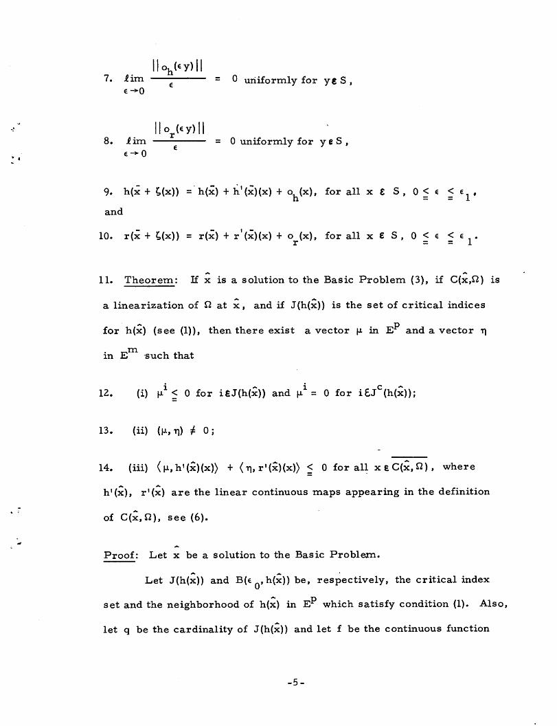
llo^yJll?• iim = 0 uniformly for y€ S ,

e-»-0

l|or(€y)||8. iim = 0 uniformly for yeS,

€->0

9. h(x + £(x)) = h(x) + h'(x)(x) + o, (x), for all x £ S , 0 < e < en ,h = = 1

and

10. r(x + £(x)) = r(x) + r'(x)(x) + o (x), for all x £ S , 0 < c < e . .r = = 1

11. Theorem: If x is a solution to the Basic Problem (3), if C(x,fi) is

a linearization of fi at x, and if J(h(x)) is the set of critical indices

for h(x) (see (1)), then there exist a vector u in E^ and a vector t|

in E such that

12. (i) v1 < 0 for i£j(h(x)) and ^=0 for i£J°(h(x));

13. (ii) (h,ti) t 0;

14. (iii) (u,h'(x)(x)) + <ti,p'(x)(x)> < 0 for all xeC(x,n), where

h'(x), r'(x) are the linear continuous maps appearing in the definition

of C(x, £2), see (6).

Proof: Let x be a solution to the Basic Problem.

Let J(h(x)) and B(e ,h(x))be, respectively, the critical index

set and the neighborhood of h(x) in Ep which satisfy condition (1). Also,

let q be the cardinality of J(h(x)) and let f be the continuous function

-5-

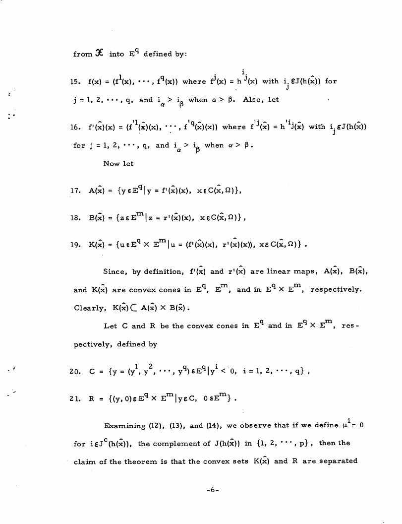
from 3£ into E defined by:

i.

15. f(x) = (t\x), •••, fq(x)) where fJ(x) =h J(x) with i. 8J(h(x)) for

j = 1, 2, • • • , q, and i > ifl when a > (3. Also, let

16. f«(x)(x) = (fa(x)(x), •••, f'q(x)(x)) where f'j(x) =h'̂ fx) with i.gJ(h(x))

for j = 1, 2, • • • , q, and i > i& when a > (3 .

Now let

17. A(x) = {yeEq|y = f'(x)(x), xgC(x,J2)},

18. B(x) = {zeEm|z = r'(x)(x), xeC(x,fl)},

19. K(x) = {ueEq X Em|u = (f'(x)(x), r'(x)(x)), xeC(x,^)} .

Since, by definition, f'(x) and r'(x) are linear maps, A(x), B(x),

and K(x) are convex cones in E, E , and in Eq X E , respectively.

Clearly, K(x) C A(x) X B(x).

Let C and R be the convex cones in Eq and in E4 X E , res -

pectively, defined by

20. C = {y = (y , y , •••, yq)BEq\yl< 0, i = 1, 2, ••• , q} ,

21. R = {(y, 0)eEq X Em|yeC, 0 £Em} .

Examining (12), (13), and (14), we observe that if we define M- = 0

for i£jC(h(x)), the complement of J(h(x)) in {1, 2, • • • , p} , then the

claim of the theorem is that the convex sets K(x) and R are separated

-6-

in E4 X E . We now construct a proof by contradiction.

Suppose that K(x) and R are not separated in EX E . We

then find that the following two statements must be true.

22. (I) The convex sets K(x) and R are not disjoint, i. e. , R I IK(x) ^ t,

the empty set.

23. (II) The convex cone B(x) in E contains the origin as an interior

point and hence B(x) = E .

Statement (II) follows from the fact that if 0 is not an interior

point of the convex set B(x), then by the separation theorem [7], it can

be separated from B(x) by a hyperplane in E , i. e. , there exists a

nonzero vector r\ in E such that

24. (r\ , z) < 0 for all z eB(x) .

Clearly, the vector (0, r\ ) in Eq X Em separates R from A(x) X B(x)

and hence from K(x), contradicting our assumption that R and K(x) are

not separated.

We now proceed to utilize the facts (I) and (II). Since the origin

in Em belongs to the non-void interior of B(x) (B(x) = E , see (II)),

we can construct a simplex 2 in B(x), with vertices z , z_, • • •, z +,»

such that

25. (i) 0 is in the interior of 2;

-7-

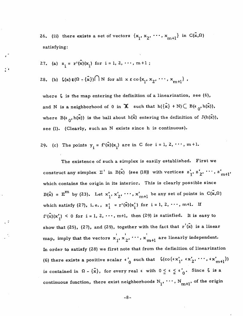
26. (ii) there exists a set of vectors {x , x_, •••, x } in C(x,£2)

satisfying:

27. (a) z. = r'(x)(x.) for i = 1, 2, • • • , m + 1 ;l i

28. (b) C(x) 8(« -{x»n Nfor all x£cofx^ x2» •••, xm+][} ,

where £ is the map entering the definition of a linearization, see (6),

and N is a neighborhood of 0 in "X such that h({x} + N) C B(e , h(x)),

where B(€ ,h(x)) is the ball about h(x) entering the definition of J(h(x)),

see (1). (Clearly, such an N exists since h is continuous).

29. (c) The points y. = f'(x)(x.) are in C for i = 1, 2, • • • , m +1.

The existence of such a simplex is easily established. First we

construct any simplex S1 in B(x) (see (18)) with vertices z^, z^, ••• , zm+1»

which contains the origin in its interior. This is clearly possible since

B(x) = Em by (23). Let x' x' , • • •, x' ,- be any set of points in C(x,£2)* ' \ L m+l

which satisfy (27), i. e. , z^ = r'(x)(xp for i = 1, 2, •••, m+l. If

f'(x)(x'.) < 0 for i = 1, 2, • • • , m+l, then (29) is satisfied. It is easy to

show that (25), (27), and (29), together with the fact that r'(x) is a linear

map, imply that the vectors x , x2» ••• , x^+1 are linearly independent.

In order to satisfy (28) we first note that from the definition of linearization

(6) there exists a positive scalar €' such that ^(cofex^ ex^, •••, €xm+1))

is contained in ^ - {x}, for every real e with 0 < € < e ' . Since ^ is a

continuous function, there exist neighborhoods N , ••• , Nm+1» of the origin

-8-

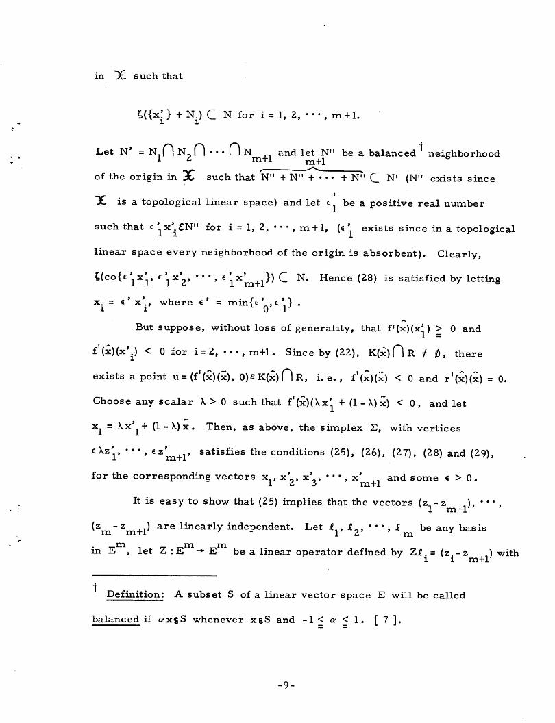
in ~%, such that

£({x!} + N.) C N for i = 1, 2, •••, m + l.

Let N* =N H N Pi ••• Pi N ,, and let N" be a balanced ' neighborhood1 2 m+l m+1

of the origin in X such that N" + N" + ••• + N" C N' (N" exists since

X is a topological linear space) and let € be a positive real number

such that €^x'.EN" for i =1, 2, •••, m+1, (€ ' exists since in a topological

linear space every neighborhood of the origin is absorbent). Clearly,

C(co{e ^x'j, e'iX'2, •••, e'x' }) C N. Hence (28) is satisfied by letting

x. = e'x\, where «' = min{e ', €*} .

But suppose, without loss of generality, that f'(x)(x') > 0 and

f'̂ Mx'..) < 0 for i=2, •-., m+l. Since by (22), K(x) 0 R t 0, there

exists a point u=(f'(x)(x), 0)sK(x)riR, i.e., f'(x)(x) < 0 and r'(x)(x) = 0.

Choose any scalar \> 0 such that f'fxKXx' + (1 - \) x) < 0, and let

xj = kx' + (l-\)x. Then, as above, the simplex 2, with vertices

ekz^, •••, ez'm+1, satisfies the conditions (25), (26), (27), (28) and (29),

for the corresponding vectors x_, x' , x' , • • • , x' ,, and some € > 0.12 3 m+l

It is easy to show that (25) implies that the vectors (z -z ), *# • ,1 m+l

(z -z .J are linearly independent. Let i_, i_, • • • , I be any basism m-ri \ c m '

in E , let Z :E -*- E be a linear operator defined by Zi. = (z.-z ) with

Definition: A subset S of a linear vector space E will be called

balanced if ffx{S whenever xgS and -l < or < l. [ 7 ].

-9-

i = 1, 2, • • • , m ; and let X : E -*• 9E be a linear operator defined by

XI. = (x. -x ,,), with i = 1, 2, ••• , m. Since the vectors (z - z ),l i m+l i m+i

i = 1, 2, • • • , m, are linearly independent, the operator Z is nonsingular.

Let Z" denote the inverse of Z . Clearly the map z -* XZ (z -zm+1)+xm+1

from 2 into co{x , x~, •••, x } is continuous.

Now, for 0 < a < 1, let S be a sphere in E with radius ap' = a

(where p > 0) and center at the origin and contained in the interior of

the simplex 2.

We now define a continuous map G from the sphere S into Er a a

by

30. GJaz) =r(x+ ^XZ^z-z^) +bx^)) ,

where ||z|| < p, az £S , and £ is the map specified by Definition (6).

From Definition (6),

31. Ga(*z) =r(x) +r' (^(.XZ^z-^) +^m+1) +or(orX Z_1(z -zm+1) +«m+1).

But r(x) = 0, r' (x) oX= Z, and r1 (x)(xm+1) =zm+1 • Hence (31)

becomes

32. GJaz) =orz +o^X Z_1(z -zm+1) +«m+1) .

|| o (aXZ^z-z ' ) +ax )\\1 r m+l m+l" _

Now, since iim = U , uniformly'a

a->0

for z6S there exists for ||z|| =p an a , 0 < aQ < 1, such that

-10-

33. 11 o (aXZ_1(z -z „) +flx ,_)|| < *p, for all 0< a < a1 r m+l m+l = 0

and 11z11 = p.

Since h satisfies (9), it is clear that the components of f may

be expanded as follows:

34. f\x + UaXZ'^z-z .,) +*x ))m+l m+l

=fte +.f^xXXZ^z -zm+1) +xm+1, +oVxZ'V -zm+1)+ oxm+1),

where || o (e z) || / e -* 0 as e -> 0 uniformly for z8S , for i =1, 2, • • • , q .

Since by construction, (see (29)), f (x)(x.) < 0 , forJ

i = 1, 2, • • •, q and j = 1, 2, • • •, m+l, and the point XZ (z-z .,) + xm+l m+l

i« - -lis in co{x., x0, • • •, x ,.} , we have f (x)(XZ (z-z ,,) + x ) < 0 ,

1 2 m+l m+l m+l

for i = 1, 2, • • •, q . Hence there exist positive real numbers a., i = l, 2, • • • , q,

such that for i = 1, 2, • • •, q, and 11 z 11 = p

35. f1(x+^(aXZ"1(z-z ,,) +ax J) < f^x) for all 0 < or < a. .m+l m+l " = i

*Let a be the minimum of {a„, a^, ar_, • • * , a } . It now follows0 12 qJ

from Brouwer's Fixed Point Theorem [ 8 ] that there exists a point a z

in S ^ such that G ^{a z ) = 0.a <**

Now, let x* = x + £(ar*XZ~ (z*- z ,.) + a-*x (1), thenm+l m+l

36. (a) r(x*) = 0 (since r(x*) = G 3je(a*z*) = 0) ,a

37. (b) x*e£2, since (x* -x)e £> (co{x , x^ •••, x^ }) C ^ - {x }.

-11-

But (35), (28), (15), and (1) imply that

38. h(x*) < h(x) and that h(x) ^ h(x*).

Now, (36), (37) and (38) contradict the assumption that x is a

solution to the Basic Problem. Therefore the'convex cones K(x) and

R are separated in E X E , i. e. , there exists a nonzero vector

(jl, r\) in E X E such that

39. (i) <|I, f'(x)(x)> + <Ti,r'(x)(x)) < 0 for all x£C(x,fi) ,

40. (ii) (jl,y> +(ti, 0) > 0 for all y£C.

But (40) implies that f1 < 0 for i = 1, 2, ••*, q . Let u=(u , ••• , up)i~

be the vector in EP defined by u J = jJiJ , i.ej(h(x)) for j = 1, 2, • • • , q and

k ci > i„, when a > |3 and u = 0 for k£j (h(x)). Hence,

a p

(i) u1 < 0 for iej(h(x)) and u1 = 0 for ieJC(h(x)),

(ii) (u,ti) 4 0,

and (39) together with the continuity of f'(x) and r'(x) yield

(iii) (u,f'(x)(x)) + <T!,r'(x)(x)> < 0 for all x£C(x,^)

-12-

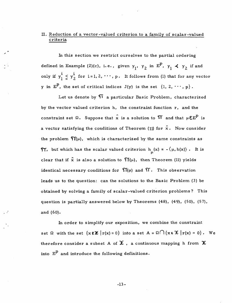
II. Reduction of a vector-valued criterion to a family of scalar-valuedcriteria

In this section we restrict ourselves to the partial ordering

defined in Example (2)(c), i.e., given y , y? in E , y -< y if and

only if y < y? for i =1, 2, • • • , p . It follows from (1) that for any vector

y in E , the set of critical indices J(y) is the set {1, 2, • • *, p} .

Let us denote by *U a particular Basic Problem, characterized

by the vector valued criterion h, the constraint function r, and the

constraint set £2. Suppose that x is a solution to TT and that u£Ep is

a vector satisfying the conditions of Theorem (11) for x. Now consider

the problem TT(n), which is characterized by the same constraints as

fT, but which has the scalar valued criterion h (x) = -(u,h(x)) . It is

clear that if x is also a solution to TT(jJ-)> then Theorem (11) yields

identical necessary conditions for TT(|J.) and TT. This observation

leads us to the question: can the solutions to the Basic Problem (3) be

obtained by solving a family of scalar-valued criterion problems? This

question is partially answered below by Theorems (48), (49), (50), (57),

and (60).

In order to simplify our exposition, we combine the constraint

set ft with the set {x8X |r(x) =0} into a set A = fiO{xtlC |r(x) = 0} . We

therefore consider a subset A of X , a continuous mapping h from 36

into Ep and introduce the following definitions.

-13-

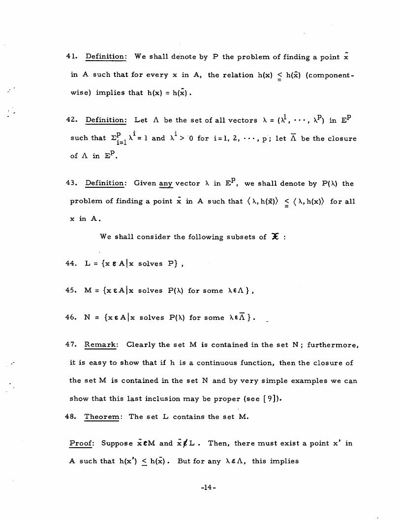
41. Definition: We shall denote by P the problem of finding a point x

in A such that for every x in A, the relation h(x) < h(x) (component

wise) implies that h(x) = h(x) .

42. Definition: Let A be the set of all vectors \ = (X.1, • • • , XP) in EP

such that 2? X. =1 and \ > 0 for i =l, 2, ••• , p ; let A be the closure

of A in EP.

43. Definition: Given any vector X. in E , we shall denote by P(M the

problem of finding a point x in A such that ( X., h(x)) < ( X., h(x)) for all

x in A.

We shall consider the following subsets of 3E :

44. L = {xeA|x solves P} ,

45. M = {xeA|x solves P(\) for some \6A},

46. N = {xeA|x solves P(X.) for some \iA } .

47. Remark: Clearly the set M is contained in the set N ; furthermore,

it is easy to show that if h is a continuous function, then the closure of

the set M is contained in the set N and by very simple examples we can

show that this last inclusion may be proper (see [9])«

48. Theorem: The set L contains the set M.

Proof: Suppose x€M and x^L . Then, there must exist a point x' in

A such that h(x') < h(x) . But for any X.£A, this implies

-14-

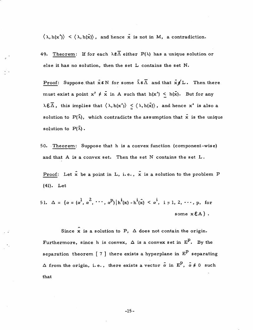
( X., h(x')) < ( X., h(x)) , and hence x is not in M, a contradiction.

49. Theorem: If for each X.EA either P(X.) has a unique solution or

else it has no solution, then the set L contains the set N.

Proof: Suppose that xfiN for some \&A and that xpL,. Then there

must exist a point xf ^ x in A such that h(x') < h(x). But for any

X.£A, this implies that ( X., h(x')) < ( X., h(x)) , and hence x* is also a

solution to P(M, which contradicts the assumption that x is the unique

solution to P(M.

50. Theorem: Suppose that h is a convex function (component-wise)

and that A is a convex set. Then the set N contains the set L.

Proof: Let x be a point in L, i.e., x is a solution to the problem P

(41). Let

•a -y • • •

51. A = {a = (a , a ,'", a^h^x) -h^x) < a1, i = 1, 2, . - • , p, for

some x£A} .

Since x is a solution to P, A does not contain the origin.

Furthermore, since h is convex, A is a convex set in E . By the

separation theorem [ 7 ] there exists a hyperplane in E separating

p -A from the origin, i. e. , there exists a vector a in E , a t 0 such

that

-15-

52. < a, a) > 0 for all at A.

Since each a can be made as large as we wish, we must have

a > 0 and hence a > 0 . For any positive scalar e > 0, let

a = h(x) -h(x) + € e for some x in A and e = (1, 1, ' * * , 1) . The vector

a is in A by definition, and hence, from (52),

53. (a,h(x) - h(x)) > -€<<*, e) .

Relation (53) holds for every x in A, and since e is arbitrary,

54. ( a, h(x) - h(x)> > 0 for all x in A.

55. If we define X = afE. ,a , then U A andi=l

56. (\,h(x)> < <\,h(x)) for all x in A.

But (55) and (56) implies that xEN.

57. Corollary: If A is convex and h is strictly convex (component

wise), then L = N.

Proof: This follows from (49) and (50).

58. Definition: We shall say that a solution x of the problem P defined

in (41), is regular if there exists a closed convex neighborhood U of x

such that for any ye A \\U the relation h(x) = h(y) implies that x = y.

-16-

59. Definition: We shall say that the problem P is regular if every

solution of P is a regular solution.

Remark: It is easy to verify that if h is convex and one if its components

is strictly convex then P is regular.

60. Theorem: Suppose that the problem P is regular, that h is

continuous and convex, and that the constraint set A is a closed convex

subset of a Hausdorff, locally convex, linear topological space IE ,

with the property that for some closed convex neighborhood V of the

origin, the set (A-{x})[ |V is compact for every x in A. Then the

set L is contained in the closure of the set M.

Proof: We shall show that for every xEL there exists a sequence of

points in M which converges to x.

We begin by constructing a sequence which converges to an

arbitrary, but fixed, x in L. We shall then show that this sequence is

in M.

Let x be any point in L. Since we can translate the origins of

^c and E , we may suppose, without loss of generality, that x = 0 and

that h(x) = 0.

Let U be a closed convex neighborhood of x satisfying the

conditions of definition (58) with respect to x, and let VC U be a

closed convex neighborhood of x such that A( |V is compact. For

-17-

any positive scalar €, 0 < e < 1/p, (where p is the dimension of the

space containing the range of h(«))i let

P

61. A(c) = {X= (X1, \2, •••, X^E^Tx1^, ^>€ for i=l, 2, •••, p} .i=l

Let g be the real-valued function with domain Al IV X A(c),

defined by

62. g(X,x) = <X,h(x)> .

Clearly, since h is continuous and convex, g is continuous in

A I IV X A(e) . Furthermore, g is convex in x for fixed X and linear

in X for fixed x. Since the sets Al IV and A(e) are compact, the sets

63. {xeAriv|g(X,x) = min g(X,n)},neAflV

64. {XeA(€)|g(X,x) = Max g(£,x)} ,geA(c)

are well defined for every X £A(«) and every xe Al IV, respectively.

Obviously, because of the form of g and because the sets Al IV and

A(c) are convex the sets defined in (63) and (64) are also convex.

By Ky Fan's Theorem [10 ], there exist a point X(e ) in A(e)

and a point x(c) in Al IV such that

-18-

65. <X,h(x(e))> < <X(€),h(x(€))> <(X(€),h(x)>

for every x in Al IV and X in A(e) .

Since x = 0 is in Al IV and h(x) = 0, we have from (65)

66. <\(€), h(x(c))> < 0,

And, from (65) and (66),

67. (X,h(x(e))> < 0 for every X in A(e).

Since Al |V is compact, we can choose a sequence € ,

n = l, 2, • • • , with 0 < € < 1/p, converging to zero in such a way thatn =

the resulting sequence of points x(e ), satisfying (65), converges, i.e.,n

68. lim x(€ ) =x*, x*eAPlV.n

n-*oo

Since g(X,x) is continuous, it follows from (67) and (68) that

69. < X,h(x*)> < 0 for all XeA,

which implies that h(x*) < 0. But x is a solution to P; hence,

h(x*) < 0 = h(x) implies that h(x*) = h(x) . Consequently, since P is

regular, x "* = x = 0. Thus, we have constructed a sequence {x(e )},

which converges to x.

We shall now show that the sequence {x(e )} contains a sub

sequence, {x(e )} also converging to x, which is contained in M.

-19-

Since x is in the interior of V, there exists a positive integer

n such that the points x(€ ) 8 Al IV belong to the interior of V for0 n

n iv

We will show that for n > nrt, x(e ) is a solution to P(X(€ )),= 0 n n

i. e. , that for n > n,_, x(e ) e M . By way of contradiction, suppose= 0 n

that for n > n , x(e ) is not a solution to P(X(e )). Then there must

exist a point x' in A such that

70. <X(6n),h(x,)> < (X(€n),h(x(en))> .

Let x"(a) = (1 -ar)x(€ ) + ax', with 0 < a < 1. Since A is convex,n

x"(a) is in A for 0 < a < 1. But for n > n^, x(e ) is in the interior= 0 n

of V, and hence there exists an a'fi, 0 < a' < 1, such that x'^a*) belongs

to V.

Now,

71. (X(€ ),h(x"(**))> = <X(e ),h((l-or*)x(e )+ ax')).n n n

But for X(€ ) eA(e ), (X(e ),h(x)) is convex in x. Hence (70)n n n

and (71) imply that

72. <X(en),h(x"(«*))> < <X(€n),h(x(6n))> ,

which contradicts (65).

Therefore, for n> n , x(c ) is a solution to P(X(e )), i.e.,

x(e ) is in M.n

-20-

Thus, for any given xeL, there exists a sequence {x(€ )}n

contained in M such that x(e ) -* x as n -* oo. This completes our

proof.

Ill -Applications to optimal control

To illustrate the applicability of the theory just developed, we

shall use it to obtain a maximum principle for an optimal control

problem with a vector-valued cost function. It will be observed that

when the vector cost function degenerates into a scalar cost function,

our maximum principle becomes identical with the Pontryagin Maximum

Principle.

Consider a dynamical system described by the differential

equation:

73. ^ =f(x,u)

for all t in the compact interval I = [t , t?], where x(t)SE is the

state of the system at time t, u(t) EE is the input of the system at

time t, and f is a function defined in E X E with range in E .

The Optimal Control Problem is that of finding a control u(t),

tSl, and a corresponding trajectory x(t), determined by (73), such

that

74. (i) for tel, u (t) is a measurable, essentially bounded function

-21-

whose range is contained in an arbitrary but fixed subset U of E ;

75. (ii) x(t ) = x , where x , a fixed vector in E , is the given

initial condition;

76. (iii) x(t2)£X2, where X_ = {xeE |g(x) = 0}, and g maps E intoI

E (X? is the fixed target set) ;

77. (iv) for every control u(t), tgl, and corresponding trajectory

x(t), satisfying the conditions (74), (75), and (76), the relation

rh ft2 -\t c(x(t), u(t))dt < \ c(x(t), u(t))dt implies that

I c(x(t), u(t))dt = 1 c(x(t), u(t)) dt , where c(x,u) maps En XE™1 1

into EP.

We make the following assumptions:

78. (i) the functions f(x, u) and c(x,u) are continuous in both x and

u, and are continuously differentiable in x ;

79. (ii) the function g(x) is continuously differentiable and the corresponding

Jacobian matrix -r?— is of maximum rank for every x in X_ .9x 2

To transcribe the control problem into the form of the Basic

Problem (3), we require the following definitions:

-22-

Let I denote the a X a identity matrix and let 0 0 denotea J ajp

the a X (3 zero matrix. We define the projection matrices P and P?

as

80. P = (I , 0^ ) ,1 p p»n

and

81. P, = (0 ,1 ).2 n,p n

Let F :EP+n X Em - EP+n be the function defined by

82. F(z,u) = (c(P2z,u), f(P2z, u)), z6EP+n, ugEm.

Now consider the differential equation

dz83. — = F(z,u)

for some u(t)£E for tel.

It is clear that the optimal control problem is equivalent to the

problem of finding a control u(t), tel and a corresponding trajectory

z(t), determined by (83), such that

84. (i) for tel, u(t) is a measurable, essentially bounded function,

whose range is contained in an arbitrary but fixed subset U of E ;

85. (ii) z(t ) = (0,x ) = z ; where x , a fixed vector in E , is the

given initial condition;

-23-

86. (iii) z(t )SX* , where X' = {z£EP n| g(P9z) = 0} , where g maps

En into E* ;

87. (iv) for every control u(t), with tel, and corresponding trajectory

z(t), satisfying (83) and the conditions (i), (ii), and (iii) above, the

relation P z(t ) < P z (t ) implies that P z(t ) = P z (t ) .

Finally, we define

88. h(z) = Pxz(t2),

89. r(z) = g(P2z(t2)),

90. and we let ft be the set of all absolutely continuous functions z

from I into E which, for some measurable, essentially bounded

function u from I into U C E , satisfy the differential equation (83)

for almost all t in I, with z(t ) = (0, x ) .

91. Remark : It is clear that with h, r, and ft defined as in (88), (89),

and (90), respectively, we have transcribed the optimal control problem

into the form of the Basic Problem (3) . We shall call the transcribed

optimal control "the optimal control problem in standard form. "

We still have not defined the linear topological space 3£ .

From (90) it is clear that ft is a subset of the linear space of all

absolutely continuous functions from I into EP . However, since we

wish to use a linearization constructed first by Pontryagin et al. [ 11 ] ,

we find it necessary to imbed ft into a larger topological linear vector

-24-

space which we define below.

Let U,be the set of all upper semi-continuous real valued

functions defined onI, and let j& = vL-XU From the properties of

upper and lower semi-continuous functions (see [12]), it follows that

J8 is a linear vector space. We then define X» to be the Cartesian

product $ = Jo x^Jx • • • x^& , with the pointwise topology, [13] i. e. ,

the topology which is constructed from the sub-base consisting of the

family of all subsets of the form { f £ X :f(t) £N}, where t is a point

in I and N is an open set in E

It is easy to show that h and r, as respectively defined by (88)

and (89), are continuous.

Let z (t), corresponding to the control u(t), be a solution to

the optimal control problem in standard form (91). We now proceed to

construct a linearization for the constraint set ft at z .

Let I,C I be the set of all points t at which u(t) is regular,

i. e. ,

n, T r.i. .. ., ,. meas (u~ (N)P)T)92. ^ ={t | ^ < t <t , lim meas (T) = l' for everymeas(T)-*0 v '

neighborhood N of u(t), teTC I } .

* 11Definition: A real valued function f : E -*E is called upper semi-

continuous at a point t in E , if lim supf(t) < f(t ). And it is calledt->t

lower semi-continuous if -f is upper semi-continuous [12].

-25-

Let $(t,T) be the (p + n) X (p + n) matrix which satisfies the

linear differential equation

d 3F - •*•93. — $ (t,T) = — (z(t), u(t))$(t,-0

for almost all t £ I, with $(t,t) = I , the (p + n) identity matrix.

For any s £ L and v e U we define

94. 6z (t) =s.v

I $(t,s)[F(z(s),v) - F(z(s), u(s))], s <t <t2 ,

and

r k95. C(z>) =} ezeX |6z(t) =S a.62s (t), {sr s2, •••, sk}C \,^- . , i' i

1=1

{v1, v2, •••, vk> C U, or. > 0, for i=1, 2, •••, k, k arbitrary

finite /.

The work by Pontryagin et al. [ 11 ] provides a proof that the

set C(z,ft) defined in (95), is a linearization for the set ft at z . The

linear maps h'(z) and r'(z) which one uses with this linearization are

defined as follows. For every 6z 6 j£ ,

0 for t < t < s

96. h'(z)(6z) = Pj&zO^)

-26-

and

8g(P2z(t ))97. r'(S)(6z) = — P26z(t2).

Therefore, from Theorem (11), there exist a vector u in E

Iand a vector r\ in E such that

98. (i) u1 < 0 for i =l, 2, •••, p;

99. (ii) (M-.-n) * 0;

9g(P2z(t )) __100. (iii) <Fi,P 6z(t2)> +<T|, ^ —P26z(t2)> < 0 for all 6z£C(z,ft)

Since every 6z (t), as defined in (94), is in C(z,ft), (100) implies' s,v

that

101. <H.,P1*(t2,8)[F(S(s),v) - F(z(s),u(s))]> +

3g(P z(t )) ^ - ^ ^+<f|. |^-=- P2$(t2,s)[F(z(s),v)-F(z(s),u(s))]> < 0

for every scl, and vSU

Hence,

102. <$ (t2,t) T T 8* <P2z(t2»*V + P2 51

for every tel , and v£U

-27-

, F(z(t),v)-F(z(t), G(t))> < 0

T T8ST(P2z(t2))103. Let i|i(t) = * (t2,t)(Px u + P2 — ti), i.e.,

for almost all t in I, ijj(t) satisfies the differential equation:

104. £ +tw . _+tw 2IJigJjai! +T(t2). ,r +nx !!W Pz.

Combining (102) and (103), we obtain

105. <i|i(t), F(z(t),u(t))> = Maximum {(i|j(t), F(z(t),v)) | veU} for t£l.

Since meas (I ) = meas (I), (105) holds for almost all t in I.

3g(P2z(t2))Remark: By assumption (see(79)), r is of maximum rank,

a x

and since (u, r|) 4- 0, ty(t) as a solution to (103) is not identically zero.

Thus, we have proved the following theorem, which we state in

terms of the original quantities defining the optimal control problem.

105. Theorem: If the control u(t) and the corresponding trajectory x(t),

tel, solve the optimal control problem, then there exist a vector

ty' eEP, ik < 0, and a vector-valued function v|j (t)eEn, with (^i* ^Mt)) # 0,

such that

d4s(t)(i) 2 = .q.T 9c(x(t),u(t)) _ T 3f(x(t),u(t)) ^dt TL 9x 2 3x

9g(x(t2))\T i(ii) ^2(t2) = ( — J r\ , for some n£E ,

-28-

(iii) for every veU and almost all t&I,

(*x, c(x(t),u(t))> +<+2(t), f(x(t), u(t))> ><^, c(x(t),v))) +<4i2(t),f(x(t),v)>

-29-

CONCLUSION

In this paper we have presented a theory of necessary conditions

for a canonical vector-valued criterion optimization problem. To

demonstrate that many complex optimization problems can be transcribed

into our canonical form, we have used our necessary conditions to con

struct a Pontryagin type maximum principle for an optimal control

problem with vector cost. It is not difficult to show that most nonlinear

programming problems of interest can also be treated within our frame

work (see [14]).

We have also considered the possibility of "scalarizing" a vector-

valued criterion problem by using convex combinations of the components

of the vector cost. Our results indicate that the solution sets of the

vector and scalar criterion problems do not necessarily coincide.

Since the conditions presented in this paper are considerably

more general than hitherto available in the literature, it is hoped that

they will open up important classes of optimization problems.

-30-

REFERENCES

1. Pareto, V. , Cours d'Economie Politique, Lausanne, Rouge, 1896.

2. Karlin, S. , Mathematical Methods and Theory in Games, Programming

and Economics, 1, Addison-Wesley, Massacnusetts, 1959.

3. Debreu, G. , Theory of Value, John Wiley, New York, 1959-

4. Kuhn, H. W. and Tucker, A. W. , "Nonlinear Programming, "

Proc. of the Second Berkeley Symposium on Mathematic Statistics

and Probability, University of California Press, Berkeley, California,

1951, pp. 481-492.

5. Zadeh, L. A. , "Optimality and Non-Scalar-Valued Performance

Criteria," IEEE Transactions on Automatic Control, vol. AC-8,

number 1, pp. 59-60; January, 1963.

6. Chang, S. S. L., "General Theory of Optimal Processes, " J. SIAM

Control, Vol. 4, No. 1, 1966, pp. 46-55.

7. Edwards, R. E. , Functional Analysis Theory and Applications, Holt

Rinehart and Winston, New York, 1965.

8. Dieudonne', J., Foundations of Modern Analysis, Academic Press,

New York, I960.

9. Klinger, A., "Vector-valued Performance Criteria," IEEE Trans

actions on Automatic Control, vol. AC-9, number 2, January 1964,

pp. 117-118.

10. Fan, K., "Fixed Point and Minimax Theorems in Locally Convex

Topological Linear Spaces, " Proc. Natl. Acad. Sci. , U. S. 38

(1952), pp. 121-126.

-31-

11. Pontryagin, L. S. et al. , The Mathematical Theory of Optimal

Processes, John Wiley, New York 1962.

12. McShane, E. J., Integration, Princeton University Press, Princeton,

1964.

13. Kelly, J. L. , General Topology, Van Nostrand, New York, 1955.

14. Da Cunha, N. O. and Polak, E. , "Constrained Minimization under

Vector-Valued Criteria in Finite Dimensional Spaces," Electronics

Research Laboratory, University of California, Berkeley, California,

Memorandum No. ERL-M188, October 1966.

15. Neustadt, L. W., "An Abstract Variational Theory with Applications

to a Broad Class of Optimization Problems II, " USCEE Report 169,

1966.

16. Halkin, H. and Neustadt, L. W. , "General Necessary Conditions

for Optimization Problems," USCEE Report 173, 1966.

17. Canon, M. , Cullum, C. and Polak, E. , "Constrained Minimization

Problems in Finite Dimensional Spaces," J. SLAM Control, Vol. 4,

No. 3, 1966, pp. 528-547.

-32-