Copy of Preuss MS thesis final - people.se.cmich.edu

PREDICTING SPATIAL DISTRIBUTION AND RELATIVE ABUNDANCE OF BOBCATS IN THE NORTHERN LOWER PENINSULA OF MICHIGAN

Timothy S. Preuss

A thesis submitted in partial fulfillment of the requirements for the degree of

Master of Science

Department of Biology

Central Michigan University Mount Pleasant, Michigan

March, 2005

ii

iii

"God made the wild animals according to their kinds... And God saw that it was good."

Genesis 1:25

iv

This is dedicated to Stephanie, my amazing wife, for her endless love, support, and encouragement.

v

ACKNOWLEDGEMENTS

I thank Central Michigan University, Defenders of Wildlife, Wildlife Forever,

Merit Energy Company, and Citgo Petroleum, Inc. for funding this research. I am

thankful to the Michigan Department of Natural Resources (MDNR) for logistic support.

I particularly thank Dan Moran of the MDNR for his committed support throughout this

research. For assistance in the field, I thank J. Conley, S. Gallagher, M. Kerr, B. Potter,

S. Preuss, H. Smith, R. Soulard, J. Stevenson, and N. Svoboda. Without the assistance of

these individuals in the field, I would not have accomplished my research objectives. I

also thank my fellow graduate students for enriching my graduate school experience. I

am particularly thankful for the new friendships I have with J. Hawley and S. Gallagher.

I am extremely thankful to my graduate advisor and friend, Dr. T. M. Gehring, for

supporting me in this research, allowing me flexibility, and always striving to provide for

my research needs. I am also thankful to my graduate committee, Dr. B. J. Swanson and

Dr. D. R. Etter, for their advice and guidance.

I am most grateful to my wife (Stephanie) and family (Dad, Mom, Dan).

Stephanie, thank you for your love, support, and encouragement; I am so proud to have

you as my wife. I will love you forever. Dad, Mom, and Dan, thank you for your love

and always supporting me in my life pursuits.

Most deserving of my thanks is Jesus Christ, my Lord and Savior, for creating

me, all those around me, and all the fauna and flora of this beautiful Earth.

vi

ABSTRACT

PREDICTING SPATIAL DISTRIBUTION AND RELATIVE ABUNDANCE OF BOBCATS IN THE NORTHERN LOWER PENINSULA OF MICHIGAN

by Timothy S. Preuss Bobcats (Lynx rufus) are a harvested furbearer species in Michigan. Controversy

over the management of bobcats in the northern Lower Peninsula of Michigan (NLP) has

stimulated a need for more information on the ecology, distribution, and abundance of

Michigan bobcats. I conducted a radio-telemetry study on bobcats in a 4,253-km2 study

area in the NLP from March 2003 – October 2004. Fifteen bobcats were live trapped,

radio collared, and monitored to investigate area requirements and habitat use. Bobcat

home ranges and core areas were estimated using minimum convex polygon and adaptive

kernel methods to determine an appropriate scale for modeling distribution and relative

abundance. I conducted scent-station surveys (n = 1400 stations) to assess bobcat

presence/absence and to aid in distribution and relative abundance modeling. I used

remotely sensed land cover data and the Penrose distance statistic to model the similarity

of habitat within core areas of radio-collared bobcats to the rest of the NLP. Bobcat core

areas were comprised of proportionately more lowland forest (51%), non-forested

wetlands (9%), and streams (3%) than the surrounding NLP.

vii

The NLP was comprised primarily of upland forest (44%) and agriculture/openland

(32%). I then modeled relative abundance and distribution based on radio-telemetry and

scent-station data. Bobcat distribution was predicted to be patchy throughout the NLP

with areas of greatest density in the northeast, central, and southeast regions of the NLP.

I validated the abundance model with an independent set of bobcat harvest locations (n =

196). The majority (75%) of independent bobcat harvest locations occurred in areas of

the NLP predicted to have greatest bobcat density. Given the current controversy over

the management of bobcats in the NLP, this model may aid state management agencies in

assessing the status of the NLP bobcat population, as well as in identifying areas

important to bobcats and areas to monitor and survey for bobcats.

viii

TABLE OF CONTENTS LIST OF TABLES .......................................................................................................... ix

LIST OF FIGURES ....................................................................................................... xii

INTRODUCTION ........................................................................................................... 1

LITERATURE CITED ........................................................................................ 4

SECTION

I. HOME-RANGE SIZE AND HABITAT USE BY BOBCATS IN THE NORTHERN LOWER PENINSULA OF MICHIGAN ................................. 6

Abstract................................................................................................... 6

Introduction............................................................................................ 6

Methods ................................................................................................... 9

Results ................................................................................................... 17

Discussion.............................................................................................. 23

LITERATURE CITED ................................................................................... 27

II. A PREDICTIVE MODEL OF BOBCAT SPATIAL DISTRIBUTION AND RELATIVE ABUNDANCE IN THE NORTHERN LOWER PENINSULA OF MICHIGAN ....................................................................... 32

Abstract................................................................................................. 32

Introduction.......................................................................................... 33

Methods ................................................................................................. 37

Results ................................................................................................... 47

Discussion.............................................................................................. 52

LITERATURE CITED ................................................................................... 59

ix

LIST OF TABLES TABLE PAGE

1. Capture data for bobcats trapped during a radio-telemetry study of bobcat home-range characteristics and habitat use in the northern Lower Peninsula, Michigan from March 2003 – July 2004 .............................. 17

2. Summer (15 May – 14 October) home-range (HR) and core-area

(CA) sizes of radio-collared bobcats in the northern Lower Peninsula, Michigan. Home ranges were calculated using the 100% minimum convex polygon (MCP) and 95% adaptive kernel (ADK) methods. Core areas were calculated using the 50% MCP and 50% ADK methods ........ 19

3. Simplified ranking matrix for radio-collared bobcats comparing

habitat composition within 95% adaptive kernel home ranges relative to habitat availability within a 4,253-km2 study area in the northern Lower Peninsula, Michigan. Cells in the matrix consist of mean differences in the log-ratios (rows divided by columns) of used and available habitats for all bobcats divided by the standard error. The sign of t-values is indicated with positive or negative signs, where a triple sign signifies nonrandom habitat use at α = 0.05. Rank is equal to the sum of positive values in each row. A larger rank value denotes a more preferred habitat type ............................................................................. 21

4. Simplified ranking matrix for radio-collared bobcats comparing

habitat composition within 50% adaptive kernel core areas relative to habitat availability within a 4,253-km2 study area in the northern Lower Peninsula, Michigan. Cells in the matrix consist of mean differences in the log-ratios (rows divided by columns) of used and available habitats for all bobcats divided by the standard error. The sign of t-values is indicated with positive or negative signs, where a triple sign signifies nonrandom habitat use at α = 0.05. Rank is equal to the sum of positive values in each row. A larger rank value denotes a more preferred habitat type ............................................................................. 21

x

TABLE PAGE

5. Simplified ranking matrix for radio-collared bobcats comparing the distribution of radio locations among habitat types within 95% adaptive kernel home ranges in the northern Lower Peninsula, Michigan. Cells in the matrix consist of mean differences in the log-ratios (rows divided by columns) of used and available habitats for all bobcats divided by the standard error. The sign of t-values is indicated with positive or negative signs, where a triple sign signifies nonrandom habitat use at α = 0.05. Rank is equal to the sum of positive values in each row. A larger rank value denotes a more preferred habitat type ...................................................... 22

6. Simplified ranking matrix for radio-collared bobcats comparing the

distribution of radio locations among habitat types within 50% adaptive kernel core areas in the northern Lower Peninsula, Michigan. Cells in the matrix consist of mean differences in the log-ratios (rows divided by columns) of used and available habitats for all bobcats divided by the standard error. The sign of t-values is indicated with positive or negative signs, where a triple sign signifies nonrandom habitat use at α = 0.05. Rank is equal to the sum of positive values in each row. A larger rank value denotes a more preferred habitat type ...................................................... 22

7. Habitat (class) and landscape variables calculated for potential use in

modeling bobcat distribution and relative abundance in the northern Lower Peninsula, Michigan. Variables were calculated using the Patch Analsyt Grid 3.0 extension for ArcView GIS. Class metrics were calculated for agriculture/openland, lowland forest, non-forested wetland, open water, streams, transportation, upland forest, and urban habitats unless noted otherwise.......................................................................... 43

8. The 11 habitat and landscape variables retained for use in the final

modeling of bobcat distribution and relative abundance in the northern Lower Peninsula, Michigan ............................................................................... 45

9. Station and transect visitation rates for bobcats and selected mammal

species detected at scent stations during surveys conducted in autumn of 2003 and 2004 .................................................................................................... 48

xi

TABLE PAGE

10. Mean values (± SE) of 11 habitat variables used for modeling distribution and relative abundance of bobcats in the northern Lower Peninsula, Michigan (NLP), and the correlations between each variable and Penrose distance (PD). Values were calculated from 50% minimum convex polygon core areas of 11 radio-collared bobcats (mean vector) and from within hexagons of a hexagon grid overlaid on the NLP. The mean habitat vector was calculated as the mean values of the 11 habitat and landscape variables within bobcat core areas. All correlations between NLP hexagon variables and Penrose distance were significant (P ≤ 0.05) .................................................... 49

xii

LIST OF FIGURES FIGURE PAGE

1. A radio-telemetry study of bobcat home-range size and habitat use was conducted between March 2003 and October 2004 in a 4,253-km2 study area in the northern Lower Peninsula, Michigan. The study area included portions of Clare, Crawford, Gladwin, Kalkaska, Missaukee, Ogemaw, Osceola, Oscoda, and Roscommon counties. The enlarged 30-m resolution study area map displays 7 habitat cover classes used for examining bobcat habitat selection (the open water cover class was excluded from habitat selection analysis) ................................ 10

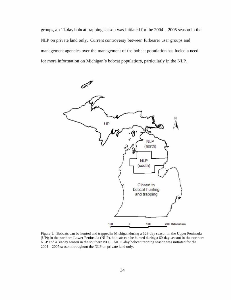
2. Bobcats can be hunted and trapped in Michigan during a 128-day

season in the Upper Peninsula (UP); in the northern Lower Peninsula (NLP), bobcats can be hunted during a 60-day season in the northern NLP and a 30-day season in the southern NLP. An 11-day bobcat trapping season was initiated for the 2004 – 2005 season throughout the NLP on private land only ............................................................................. 34

3. Location of the 4,253-km2 study area in the northern Lower Peninsula, Michigan (NLP. A radio-telemetry study was conducted assessing bobcat area requirements and habitat use to aid in spatially modeling bobcat distribution and relative abundance throughout the NLP. The enlarged 30-m resolution study area map displays 8 habitat cover classes ...................... 38

4. Location of the 48,518-km2 northern Lower Peninsula, Michigan (NLP).

A model of bobcat distribution and relative abundance was developed for the NLP using 8 habitat cover classes identified in the enlarged 30-m resolution map.................................................................................................... 38

xiii

FIGURE PAGE

5. Scent-station surveys were conducted in autumn of 2003 and 2004 to provide presence/absence data in order to supplement radio-telemetry locations for use in relative abundance and distribution modeling. Scent-station transects (represented by yellow lines) were placed along paved and unpaved roads and 2-track forest trails throughout and adjacent to the study area (represented by the black polygon) .................................................................... 41

6. Hexagon grid overlaid on land-cover of the northern Lower

Peninsula, Michigan. Habitat and landscape variables were calculated within each 5.1-km2 hexagon (i.e., equivalent to the size of an average adult bobcat core area) for modeling bobcat distribution and relative abundance ................................................................... 42

7. Penrose distance map depicting habitat similarity between core areas

of radio-collared adult bobcats and the northern Lower Peninsula, Michigan. Lower Penrose distance values indicate a greater similarity of habitat to bobcat core areas............................................................................ 50

8. Map of the northern Lower Peninsula, Michigan (NLP) depicting

predicted relative abundance of bobcats throughout the region. Bobcat abundance is based on a relationship between the similarity of habitat in the NLP to the habitat characteristics of bobcat core areas and abundance information from radio-collared bobcats and scent-station surveys .......................................................................................... 51

9. Map of bobcat relative abundance in the northern Lower Peninsula,

Michigan with locations of 196 bobcats harvested during the 2002 – 2003 Michigan bobcat hunting season. Locations from harvested bobcats were used for model validation. The area south and west of the yellow line is closed to bobcat hunting.......................................................................... 52

1

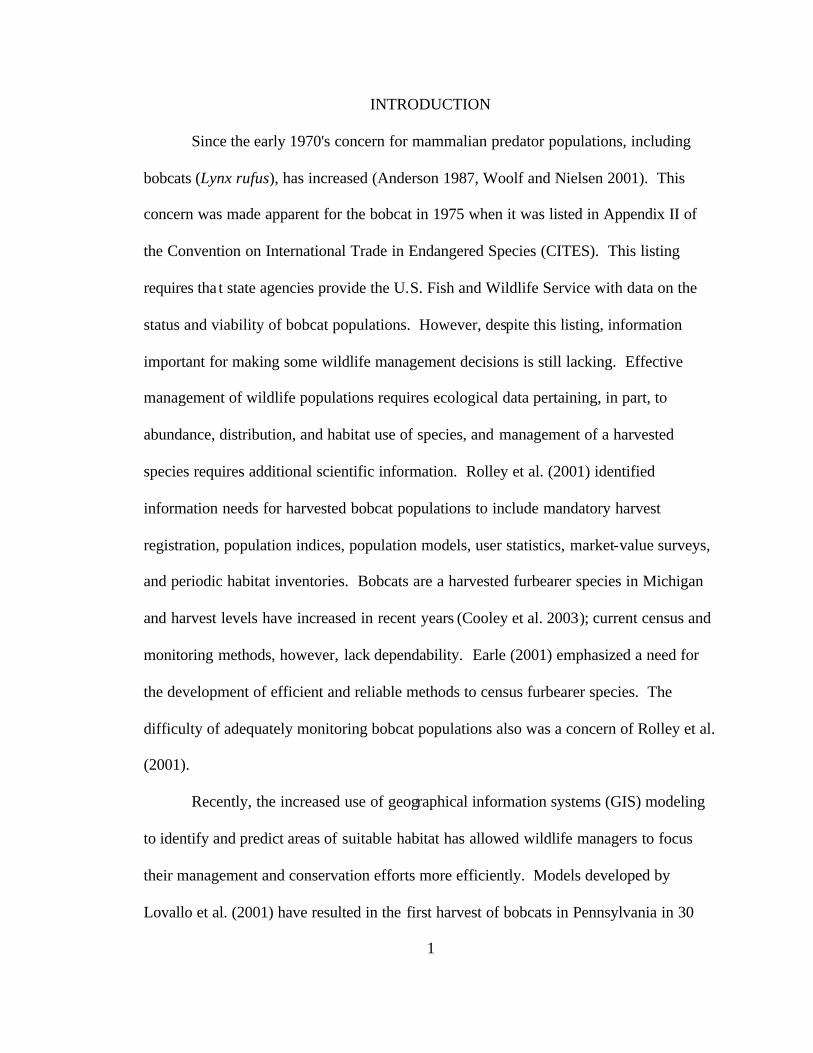
INTRODUCTION

Since the early 1970's concern for mammalian predator populations, including

bobcats (Lynx rufus), has increased (Anderson 1987, Woolf and Nielsen 2001). This

concern was made apparent for the bobcat in 1975 when it was listed in Appendix II of

the Convention on International Trade in Endangered Species (CITES). This listing

requires tha t state agencies provide the U.S. Fish and Wildlife Service with data on the

status and viability of bobcat populations. However, despite this listing, information

important for making some wildlife management decisions is still lacking. Effective

management of wildlife populations requires ecological data pertaining, in part, to

abundance, distribution, and habitat use of species, and management of a harvested

species requires additional scientific information. Rolley et al. (2001) identified

information needs for harvested bobcat populations to include mandatory harvest

registration, population indices, population models, user statistics, market-value surveys,

and periodic habitat inventories. Bobcats are a harvested furbearer species in Michigan

and harvest levels have increased in recent years (Cooley et al. 2003); current census and

monitoring methods, however, lack dependability. Earle (2001) emphasized a need for

the development of efficient and reliable methods to census furbearer species. The

difficulty of adequately monitoring bobcat populations also was a concern of Rolley et al.

(2001).

Recently, the increased use of geographical information systems (GIS) modeling

to identify and predict areas of suitable habitat has allowed wildlife managers to focus

their management and conservation efforts more efficiently. Models developed by

Lovallo et al. (2001) have resulted in the first harvest of bobcats in Pennsylvania in 30

2

years. Nielson and Woolf (2002) developed models that linked habitat and relative

abundance to evaluate distribution and abundance of bobcats in Illinois. These models

were used to assess bobcat status and contributed to the delisting of bobcats as a

threatened species in Illinois (Woolf et al. 2002). Integrating demographic data (e.g.,

data determined via telemetry methods) and GIS spatial models can provide a tool to

focus management efforts. These tools are rare for management of bobcats and other

solitary carnivores. Region specific models should be developed to more effectively

direct bobcat management (Lovallo et al. 2001).

In Section 1, I investigate home-range attributes and patterns of habitat use for

bobcats in the northern Lower Peninsula, Michigan (NLP). My objectives were to

estimate home-range and core-area size for female and male bobcats, and assess the use

and selection of habitats by bobcats in the NLP. I predicted that average home-range and

core-area size would be larger for male than for female bobcats. In the Great Lakes

Region, intersexual differences occur in the degree to which bobcats are territorial

(Lovallo and Anderson 1996). Female bobcats typically have smaller home ranges and

exclude other females from their territory. This behavior likely reduces competition (e.g.,

energy consumption) with other females during periods when energy needs are critical

(e.g., kitten rearing). Male bobcats, however, appear to be less territorial toward other

males, yet have large home ranges encompassing several female home ranges in order to

increase mating opportunities with females. Additionally, I predicted that bobcats would

utilize habitats disproportionately to their occurrence. Habitats that are more suitable

(e.g., high prey density, available den sites, fewer competitors) are likely to be preferred.

In the Great Lakes Region, bobcats are known to prefer lowland conifer forests due to the

3

availability of prey species as well as the thermal cover provided (Berg 1979, Fuller et al.

1985, Lovallo and Anderson 1996).

In Section 2, I develop a computer-based model to predict the abundance and

distribution of bobcats in the NLP. My objective was to integrate assessments of home-

range dynamics and habitat use (Section 1) with digital land-cover data to predict bobcat

distribution and relative abundance throughout the NLP. I predicted that bobcat

abundance and distribution would be linked primarily to variables associated with

lowland forest cover. Lowland forests have been shown to be an important component of

bobcat home ranges in Wisconsin (Lovallo and Anderson 1996) and Minnesota (Berg

1979, Fuller et al. 1985), as well as in Michigan (Section 1). A predictive spatial model

would provide wildlife managers with information on bobcat distribution and suitable

bobcat habitat throughout the NLP. Additionally, wildlife managers could use such a

model to identify areas in which to focus management and monitoring efforts in order to

promote bobcat conservation.

4

LITERATURE CITED

Anderson, E. M. 1987. A critical review and annotated bibliography of literature on the

bobcat. Terrestrial Wildlife Research Report 62, Colorado Division of Wildlife,

Denver, Colorado, USA.

Berg, W. E. 1979. Ecology of bobcats in northern Minnesota. Pages 55-61 in P.C.

Escherich and L. Blum, editors. Proceedings of the 1979 bobcat research

conference (Science and Technology Series 6). National Wildlife Federation,

Washington D.C., USA.

Cooley, T. M., S. M. Schmitt, P. D. Friedrich, and T. F. Reis. 2003. Bobcat survey

2002-2003. Michigan Department of Natural Resources. Wildlife Report No.

3400.

Earle, R. D. 2001. Furbearer winter track count survey of 2000. Michigan Department

of Natural Resources. Wildlife Report No. 3331.

Fuller, T. K., D. W. Kuehn, and W. E. Berg. 1985. Bobcat home range size and daytime

cover-type use in Northcentral Minnesota. Journal of Mammalogy 66:568-571.

Lovallo, M. J., and E. M. Anderson. 1996. Bobcat (Lynx rufus) home range size and

habitat use in northwest Wisconsin. American Midland Naturalist 135:241-252.

Lovallo, M. J., G. L. Storm, D. S. Klute, and W. M. Tzilkowski. 2001. Multivariate

models of bobcat habitat selection for Pennsylvania landscapes. Pages 4-17 in

A.Woolf, C. K. Nielsen, and R. D. Bluett, editors. Proceedings of a symposium

on current bobcat research and implications for management. The Wildlife

Society 2000 Conference, Nashville, Tennessee, USA.

5

Nielsen, C. K., and A. Woolf. 2002. Habitat-relative abundance relationship for bobcats

in southern Illinois. Wildlife Society Bulletin 30:222-230.

Rolley, R. E., B. E. Kohn, and J. F. Olson. 2001. Evolution of Wisconsin's bobcat

harvest management program. Pages 61-66 in A.Woolf, C. K. Nielsen, and R. D.

Bluett, editors. Proceedings of a symposium on current bobcat research and

implications for management. The Wildlife Society 2000 Conference, Nashville,

Tennessee, USA.

Woolf, A., and C. K. Nielsen. 2001. Bobcat research and management: have we met the

challenge? Pages 1-3 in A.Woolf, C. K. Nielsen, and R. D. Bluett, editors.

Proceedings of a symposium on current bobcat research and implications for

management. The Wildlife Society 2000 Conference, Nashville, Tennessee,

USA.

Woolf, A., C. K. Nielsen, T. Weber, and T. J. Gibbs-Kieninger. 2002. Statewide

modeling of bobcat, Lynx rufus, habitat in Illinois, USA. Biological Conservation

104:191-198.

6

SECTION I

HOME-RANGE SIZE AND HABITAT USE BY BOBCATS IN THE NORTHERN LOWER PENINSULA OF MICHIGAN

Abstract

Controversy over the management of bobcats in the northern Lower Peninsula,

Michigan (NLP) has stimulated a need for more information on the ecology of Michigan

bobcats. I conducted a radio-telemetry study on bobcats in the NLP from March 2003 –

October 2004. Fifteen bobcats were live trapped, radio collared, and monitored to

examine home-range characteristics and habitat use. Home ranges of male bobcats were

>3 times larger than those of females (Z = -2.74, P = 0.006). Analysis of habitat use

indicated that bobcats selected lowland coniferous forest, lowland deciduous forest, and

non-forested wetland habitats, while upland forest, urban, and open habitats were

avoided. The identification of bobcat area requirements and habitat needs may aid

biologists in management efforts.

Introduction

Since 1975 when bobcats (Lynx rufus) were added as a “threatened look-alike”

species to Appendix II of the Convention on International Trade in Endangered Species

(CITES), studies on bobcat ecology and behavior have increased substantially generating

a wealth of information on bobcats. However, since bobcats are widely distributed

throughout much of North America it is difficult to extrapolate data from region to

region. Bobcat home-range size and overlap, as well as habitat use, are particularly

variable throughout the bobcat’s distribution. In general, home ranges of bobcats in the

northern latitudes are substantially larger than those in southern latitudes, likely due to

7

lower prey abundance and increased thermal demands in the northern regions (Anderson

and Lovallo 2003). In Maine, male bobcat home ranges averaged 112 km2 (Litvaitis et

al. 1987), however home ranges of male bobcats in Alabama averaged 2.6 km2 (Miller

and Speake 1979). Additionally, home ranges of male bobcats are typically 2 to 3 times

larger than female home ranges (Anderson and Lovallo 2003). In the southern regions,

female bobcats usually maintain exclusive home ranges, while male bobcat home ranges

overlap minimally (Miller and Speake 1979, Rolley 1985). In these regions, bobcats are

able to keep intrasexually exclusive home ranges while maintaining relatively high

densities (Miller and Speake 1979). In the northern regions, female bobcats are also

likely to maintain exclusive home ranges, however home ranges of males tend to overlap

extensively with other males and encompass the home ranges of 2 or 3 females (Lovallo

and Anderson 1996a). In these regions bobcats typically occur at lower densities

compared to bobcats in southern regions, likely due to prey resources that are not usually

as abundant in harsher climates (Bailey 1981). However, the understanding of bobcat

home-range dynamics may be confounded depending on the presence or absence of a

harvest (e.g., hunting and/or trapping). Rolley (1985) observed no intrasexual overlap in

home ranges of male and female bobcats in a harvested population in Oklahoma.

However, in the absence of a harvest, male and female bobcats in southern Illinois

exhibited a high degree of intrasexual overlap (Nielson and Woolf 2001). It is important

to understand home-range dynamics in order to effectively manage bobcat populations,

particularly harvested populations.

Bobcat habitat use also varies greatly throughout its geographic distribution, and

appears to be focused in habitats that provide abundant prey and allow for hunting by

8

either ambush or stalking (Anderson and Lovallo 2003). In Minnesota and Wisconsin,

lowland coniferous forests were preferred habitat for bobcats (Fuller et al. 1985, Lovallo

and Anderson 1996a). Bobcat habitat use in Maine included hardwood and coniferous

forests depending on the density of the understory layer (Litvaitis et al. 1986).

Additionally, bobcats in the southeast tend to prefer bottomland forests, whereas bobcats

in the west are found most often in dry, rocky habitats (Anderson and Lovallo 2003).

Identifying habitats that provide the necessary resources for bobcats is important in order

to identify areas that should be conserved, or preserved, particularly when these types of

habitat are scarce (Fuller et al. 1985).

Few studies exist on bobcat home-range size and habitat use in the Great Lakes

region (Erickson 1955, Berg 1979, Fuller et al. 1985, Lovallo and Anderson 1996a).

Erickson (1955) used winter snow tracking methods to investigate home-range size and

habitat use by bobcats in Michigan, however current quantitative data on bobcat home-

range characteristics and habitat use is lacking for Michigan, particularly in the northern

Lower Peninsula (NLP). The extensive geographic variability in bobcat ecology makes

the extrapolation of population characteristics between regions problematic (Anderson

and Lovallo 2003). Furthermore, local dynamics (e.g., hunting and trapping pressure,

levels of human encroachment, levels of habitat fragmentation, and management

strategies) also make the extrapolation of population characteristics between states within

a region troublesome. Data on bobcat habitat use in Michigan is collected from winter

track surveys in the Upper Peninsula (UP; Earle 2001). Habitat use information from

these data is difficult to extrapolate to the NLP because habitat composition varies

somewhat between the UP and NLP, and road density, area of land in agricultural

9

production, and level of urbanization are much greater in the NLP. Additionally, bobcats

are a harvested furbearer species in Michigan. The UP experiences greater harvest

pressure than the NLP resulting in greater numbers of bobcats being harvested in the UP

as compared to the NLP (Cooley et al. 2003, Frawley et al. 2004).

I conducted a radio-telemetry study from March 2003 – October 2004 to assess

area and habitat requirements of bobcats in the NLP. The objectives were to: 1) estimate

home-range and core-area size for female and male bobcats; and 2) assess the use and

selection of habitats by bobcats.

Methods

Study Area

The 4,253-km2 study area included portions of Clare, Crawford, Gladwin,

Kalkaska, Missaukee, Ogemaw, Osceola, Oscoda, and Roscommon counties, Michigan

(Figure 1). I delineated the study area by extending a 17-km buffer (equivalent to the

length of the longest adult bobcat home range from this study) around the outermost

home ranges of radio-collared bobcats. I obtained 2001 IFMAP/GAP Lower Peninsula

Land Cover data with 30-m resolution developed by the Forest, Mineral, and Fire

Management Division of the Michigan Department of Natural Resources (MDNR). I

reclassified the original 32 cover classes into 8 major cover classes using ArcGIS 8.3

(Environmental Systems Research Institute, Redlands, California, USA). I identified

cover classes in the study area as: agriculture/openland (28%), lowland coniferous forest

(6%), lowland deciduous forest (5%), non-forested wetland (4%), open water (4%),

upland coniferous forest (22%), upland deciduous forest (29%), and urban/transportation

10

(2%). Forested areas were dominated by oak (Quercus spp.), aspen (Populus spp.), and

mixed pine (Pinus spp.) on upland sites and northern white cedar (Thuja occidentalis)

and balsam fir (Abies balsamea) on lowland sites (Leatherberry 1994).

Figure 1. A radio-telemetry study of bobcat home-range size and habitat use was conducted between March 2003 and October 2004 in a 4,253-km2 study area in the northern Lower Peninsula, Michigan. The study area included portions of Clare, Crawford, Gladwin, Kalkaska, Missaukee, Ogemaw, Osceola, Oscoda, and Roscommon counties. The enlarged 30-m resolution study area map displays 7 habitat cover classes used for examining bobcat habitat selection (the open water cover class was excluded from habitat selection analysis).

Trapping

Bobcats were trapped during 2 trapping periods from March – July 2003 and May

– July 2004. Model 209.5 Tomahawk® cage traps (Tomahawk Live Trap, Tomahawk,

Wisconsin, USA) and #3 Victor Soft-Catch® padded foot-hold traps (Oneida Victor, Inc.,

Euclid, Ohio, USA) were used in 2003, and foot-hold traps were used exclusively in

2004. Cage traps were made of galvanized wire mesh and measured 38 x 50 x 107 cm.

Each foot-hold trap was modified (Earle et al. 2003), attached to a 183-cm chain with

11

drag, and double swivels were placed between the trap and chain, half way between the

trap and drag, and between the chain and drag. Traps were selectively placed in areas

known or suspected to support bobcats. Cage traps were covered with balsam fir boughs

and baited with combinations of bobcat urine, commercial trapping lures, meat baits, and

visual attractants. Foot-hold traps were placed in blind sets, cubby sets, dirt-hole sets,

and urine-post sets. Cubby sets and dirt-hole sets were baited with combinations of

bobcat urine, commercial trapping lures, meat baits, and visual attractants. Traps were

checked daily and the status of each trap was recorded. Trap-nights of operation were

calculated for each trapping period.

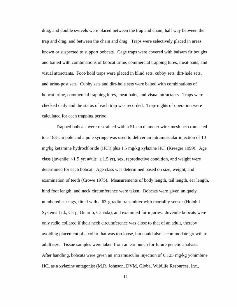
Trapped bobcats were restrained with a 51-cm diameter wire-mesh net connected

to a 183-cm pole and a pole syringe was used to deliver an intramuscular injection of 10

mg/kg ketamine hydrochloride (HCl) plus 1.5 mg/kg xylazine HCl (Kreeger 1999). Age

class (juvenile: <1.5 yr; adult: ≥ 1.5 yr), sex, reproductive condition, and weight were

determined for each bobcat. Age class was determined based on size, weight, and

examination of teeth (Crowe 1975). Measurements of body length, tail length, ear length,

hind foot length, and neck circumference were taken. Bobcats were given uniquely

numbered ear tags, fitted with a 63-g radio transmitter with mortality sensor (Holohil

Systems Ltd., Carp, Ontario, Canada), and examined for injuries. Juvenile bobcats were

only radio collared if their neck circumference was close to that of an adult, thereby

avoiding placement of a collar that was too loose, but could also accommodate growth to

adult size. Tissue samples were taken from an ear punch for future genetic analysis.

After handling, bobcats were given an intramuscular injection of 0.125 mg/kg yohimbine

HCl as a xylazine antagonist (M.R. Johnson, DVM, Global Wildlife Resources, Inc.,

12

personal communication). Bobcats were placed in a cage trap and allowed to recover in a

secluded, shaded area. Bobcats were released when they appeared fully alert. Procedures

used to trap and handle bobcats were conducted under permit from the MDNR (SC 1172)

and approved by the Institutional Animal Care and Use Committee of Central Michigan

University (IACUC# 03-03).

Radio Telemetry

Radio-collared bobcats were located by triangulation using standard telemetry

techniques (White and Garrott 1990). Aerial telemetry was used to locate missing

animals. Bobcats were located 0-3 times/24-hr period from May 2003 – October 2004

using a vehicle-mounted, 4-element Yagi directional antenna and an electronic compass

(Lovallo et al. 1994). Telemetry bearing error (2.5°) was determined by taking bearings

to reference transmitters (n = 30) placed at known locations. All bearings for bobcat

location estimates were obtained within 20 min to reduce error related to animal

movement. I attempted to obtain locations at randomly determined times to provide a

representative sample of bobcat habitat use. Locations for individual bobcats were taken

>4 hr apart to achieve independence of successive locations. The level of autocorrelation

between successive locations would likely be negligible at this interval (Swihart and

Slade 1985a, 1985b). Locations were estimated using ≥ 2 bearings. Locations and

associated error polygons were estimated with ≥ 3 bearings using the maximum

likelihood estimator (Lenth 1981) in the software program LOCATE II (Nams 1990).

For locations obtained with only 2 bearings, I attempted to maintain an angle of

intersection near 90º to minimize error (White and Garrott 1990). For data analyses, I

13

classified bobcat locations based on sex and biological season. Biological seasons

(summer = 15 May to 14 October, winter = 15 October to 14 May) were defined

according to the reproductive biology of bobcats (Lovallo and Anderson 1996a). In

summer, female bobcats are typically rearing young which suggests that a female’s

home-range size and use of habitat may be influenced by the presence of kittens. In

winter when the majority of bobcat breeding occurs, females are generally protecting

their home ranges from other females, while males are seeking mating opportunities. In

addition, prey resources may be scarce during winter forcing bobcats to expand their

home range in search of food. Only data from adult bobcats were used in analyses.

Juvenile bobcats were excluded from analyses because their use of the landscape was not

expected to represent that of a resident individual.

Home Range

I estimated the size of bobcat summer home ranges and core areas using the

minimum convex polygon (MCP; Mohr 1947) and adaptive kernel (ADK; Worton 1989)

methods. I estimated home ranges and core areas using the Home Range Extension for

ArcView GIS (Rodgers and Carr 1998). Specifically, I estimated 50% core areas and

100% home ranges using the MCP method for comparison with previous studies. I

estimated 50% ADK core areas and 95% ADK home ranges because the adaptive kernel

method of home-range estimation is robust to violations of independence (Swihart and

Slade 1985a, 1985b, 1997). The MCP estimator of home-range size is perhaps the most

common method of depicting range size and shape (Harris et al. 1990). Minimum

convex polygon estimates are obtained by connecting the outermost locations of a set of

14

locations for an individual animal. The only constraint with this method is that the

polygon formed remains convex. However, the MCP method has substantial

disadvantages despite the simplicity and common usage of the method (White and

Garrott 1990). The MCP method does not account for the intensity at which an animal

uses different parts of its range (Kenward 2001). Additionally, since animals

occasionally make excursions (e.g., to breed) outside of their normal home range,

minimum convex polygons often contain large areas which animals never use (Kenward

2001). The ADK estimator, although complex to compute, provides an improved method

of home-range estimation. The ADK method is a function based on the density of

locations for an individual animal and provides a more representative estimation of how

intensively an animal uses different parts of its home range (Worton 1989). Also, since

the ADK method allows the contribution of each point location to the overall home-range

estimate to be weighted individually based on the density of nearby points, a more

accurate depiction of the distribution of locations (i.e., home-range estimate) can be

achieved. A disadvantage of the ADK estimator, however, is that it tends to slightly

overestimate an animal’s peripheral use of its home range (Seaman 1999, Powell 2000).

To assess whether home-range estimates achieved stability, I plotted home-range area

against number of locations for each adult bobcat (Kenward 2001). Adult bobcats that

did not have enough locations to achieve home-range stability were excluded from

analysis. I used the Mann-Whitney test (α = 0.05) to assess differences in home-range

and core-area size of female and male bobcats (Zar 1999).

15

Habitat Use

I examined bobcat summer use of 7 major habitat aggregations:

agriculture/openland, lowland coniferous forest, lowland deciduous forest, non-forested

wetland, upland coniferous forest, upland deciduous forest, and urban/transportation

(Figure 1). I used theme overlay routines in ArcView 3.2 (Environmental Systems

Research Institute, Redlands, California, USA) to estimate the proportion of used habitat

within 95% ADK home ranges and 50% ADK core areas compared to available habitat in

the study area. I also calculated the proportion of telemetry point locations for each

bobcat occurring within each habitat type for comparison with available habitat within

95% ADK home ranges and 50% ADK core areas. Point locations with an error ellipse

encompassing more than 1 habitat type were excluded from analysis to avoid assignment

of locations to unused habitats. I also refrained from using the proportion of each habitat

type occurring within an error ellipse because in some instances use could be heavily

weighted toward an unused habitat. For example, a point location with a large error

ellipse may be comprised of agriculture/openland and lowland coniferous forest. If the

lowland coniferous forest occurred as a thin riparian corridor in the middle of a large

agricultural field, the agriculture/openland habitat type would comprise the majority of

the error ellipse. But, if the bobcat was using the riparian corridor consisting of lowland

coniferous forest and not the agricultural field, then the agriculture/openland habitat type

would be falsely weighted in terms of habitat use when identifying used habitat based on

the proportion of each habitat type comprising the error ellipse.

I used compositional analysis to investigate landscape-, home range-, and core

area-level patterns of habitat selection by bobcats (Aebischer et al. 1993). An advantage

16

of compositional analysis is that it allows for the assessment of habitat use at different

levels of selection. Johnson (1980) identified 4 levels, or orders, of habitat selection: 1)

first-order selection is defined as the selection of a geographical range of a species; 2)

second-order selection is defined as the selection, or placement, of an individual’s home

range within a larger landscape; 3) third-order selection pertains to the extent at which an

individual uses the various habitat components of its home range; and 4) fourth-order

selection pertains to the behavior associated with a particular habitat component (e.g., if

third-order selection determines a particular feeding site, the procurement of food items

from that feeding site can be termed fourth-order selection). I examined second-order

selection by comparing the habitat composition of home ranges and core areas to

available habitat in the surrounding landscape (i.e., the study area). I examined third-

order selection by comparing the proportion of radio-telemetry locations occurring within

each habitat type to available habitat in home ranges and core areas for individual

bobcats. I used code provided by Ott and Hovey (1997) to perform compositional

analysis in SAS (SAS Institute Inc., Cary, North Carolina, USA). Compositional analysis

has several advantages over other types of habitat selection analyses. Compositional

analysis treats the animal, rather than the location, as the experimental unit (i.e.,

independence of radio locations is not required), thereby circumventing problems related

to pseudoreplication (Hurlbert 1984, Aebischer et al. 1993). Additionally, compositional

analysis overcomes problems pertaining to sampling level (Kenward 1992), non-

independence of proportions (i.e., avoidance of 1 habitat type inevitably leads to selection

of another), differential use of habitat by groups of individuals (e.g., females may use

habitat differently than males), and arbitrary definition of habitat availability (Aebischer

17

et al. 1993). As recommended by Aebischer et al. (1993), I substituted 0.01% for habitat

types that were available but not used by bobcats (natural zeros), whereas structural zeros

(unavailable habitat types) were eliminated by excluding these habitat types from further

analysis. For a given habitat type, I summed across available habitats the number of

positive t-values (i.e., the mean difference in the log-ratio of used and available habitats

divided by the standard error). I then ranked habitat types by the number of positive

values, where a larger rank value indicated a more preferred habitat.

Results

Trapping

I captured and radio-collared a total of 15 bobcats (Table 1). Thirteen bobcats

Table 1. Capture data for bobcats trapped during a radio-telemetry study of bobcat home-range characteristics and habitat use in the northern Lower Peninsula, Michigan from March 2003 – July 2004. Bobcat Weight Date ID Sex (kg) Age Captured Trap type Status

F01 F 5.9 Adult 5/20/03 Foot-hold Active


F03 F 6.4 Adult 6/06/03 Foot-hold Missing

F04 F 7.3 Adult 6/12/03 Foot-hold Hit by car


M01 M 14.1 Adult 5/15/03 Cage Missing

M02 M 10.9 Adult 5/26/03 Foot-hold Txa malfunction

M03 M 13.2 Adult 6/16/03 Foot-hold Active

M04 M 11.7 Adult 5/11/04 Foot-hold Missing M05 M 11.7 Adult 5/15/04 Foot-hold Active

M06 M 8.3 Juvenile 5/20/04 Foot-hold Tx malfunction

M07 M 6.5 Juvenile 5/22/04 Foot-hold Active




a Transmitter

18

were captured in foot-hold traps during 2,383 trap nights, 1 bobcat was caught in a cage

trap during 1,248 trap nights, and 1 bobcat was acquired as an incidental capture by U.S.

Department of Agriculture personnel. In 2003, trapping success was 1 bobcat per 270

foot-hold trap nights, whereas cage traps recorded 1 bobcat capture in 1,248 trap nights.

In 2004, trapping success was 1 bobcat per 113 foot-hold trap nights. Thirteen (5 females

and 8 males) of the 15 bobcats captured and radio collared were classified as adults. Two

other males were classified as juveniles.

Radio Telemetry

I obtained 915 locations on 13 adult bobcats from May 2003 through October

2004. Triangulations accounted for 90% of all locations; the remaining 10% of locations

were obtained from 2 bearings (8%) and via aerial telemetry (2%). Triangulated

locations had an average bearing error of 1.0º ± 2.6 ( x ± SD) and location error polygons

of 0.03 km2 ± 0.18 ( x ± SD). The average number of locations per bobcat was 70 (range:

12-145), and bobcats were monitored an average of 230 (range: 14-504) days.

Approximately 71% of locations were obtained during diurnal hours (0900 to 1700) with

the remaining 29% of locations obtained during crepuscular and nocturnal hours (1700 to

0900). The majority of locations (87%) were obtained during the summer season while

13% of locations were obtained in winter. Eleven of the 13 adult bobcats were monitored

through at least 1 summer season; only five adult bobcats (4 females and 1 male) were

radio-monitored through 2 summers (1 winter). Consequently, due to sample size

concerns, subsequent analyses of home range and habitat use only examine the summer

season. Furthermore, males and females were pooled for habitat use analysis.

19

At the end of the study, 9 bobcats (3 females and 6 males) were active, 1 female

had been hit by a car, and the status of 5 individuals was unknown (missing or transmitter

malfunction).

Home Range

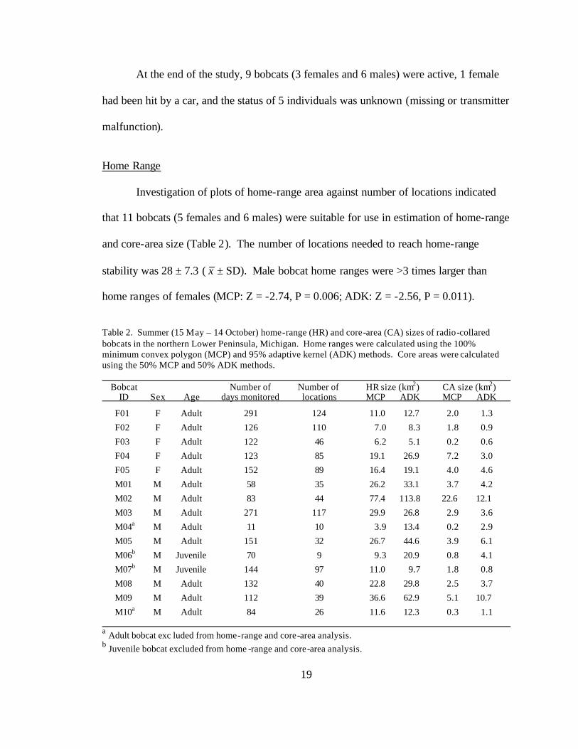
Investigation of plots of home-range area against number of locations indicated

that 11 bobcats (5 females and 6 males) were suitable for use in estimation of home-range

and core-area size (Table 2). The number of locations needed to reach home-range

stability was 28 ± 7.3 ( x ± SD). Male bobcat home ranges were >3 times larger than

home ranges of females (MCP: Z = -2.74, P = 0.006; ADK: Z = -2.56, P = 0.011).

Table 2. Summer (15 May – 14 October) home-range (HR) and core-area (CA) sizes of radio-collared bobcats in the northern Lower Peninsula, Michigan. Home ranges were calculated using the 100% minimum convex polygon (MCP) and 95% adaptive kernel (ADK) methods. Core areas were calculated using the 50% MCP and 50% ADK methods. Bobcat Number of Number of HR size (km2) CA size (km2) ID Sex Age days monitored locations MCP ADK MCP ADK

F01 F Adult 291 124 11.0 12.7 2.0 1.3

F02 F Adult 126 110 7.0 8.3 1.8 0.9

F03 F Adult 122 46 6.2 5.1 0.2 0.6

F04 F Adult 123 85 19.1 26.9 7.2 3.0

F05 F Adult 152 89 16.4 19.1 4.0 4.6

M01 M Adult 58 35 26.2 33.1 3.7 4.2

M02 M Adult 83 44 77.4 113.8 22.6 12.1

M03 M Adult 271 117 29.9 26.8 2.9 3.6

M04a M Adult 11 10 3.9 13.4 0.2 2.9

M05 M Adult 151 32 26.7 44.6 3.9 6.1

M06b M Juvenile 70 9 9.3 20.9 0.8 4.1

M07b M Juvenile 144 97 11.0 9.7 1.8 0.8

M08 M Adult 132 40 22.8 29.8 2.5 3.7

M09 M Adult 112 39 36.6 62.9 5.1 10.7

M10a M Adult 84 26 11.6 12.3 0.3 1.1

a Adult bobcat exc luded from home-range and core-area analysis. b Juvenile bobcat excluded from home -range and core-area analysis.

20

Minimum convex polygon estimates of mean home-range size for female and male

bobcats were 11.9 km2 ± 5.7 ( x ± SD) and 36.6 km2 ± 20.5 ( x ± SD), respectively. Mean

home-range size using 95% ADK contours were 14.4 km2 ± 8.7 ( x ± SD) and 51.8 km2 ±

33.1 ( x ± SD) for females and males, respectively. Male bobcat core areas were also >3

times larger than female core areas, however that difference was only significant in 50%

ADK contours (Z = -2.19, P = 0.028), but not for 50% MCP core areas (Z = -1.10, P =

0.273). Female and male core-area estimates averaged 3.0 km2 ± 2.7 ( x ± SD) and 6.8

km2 ± 7.8 ( x ± SD), respectively for 50% MCP estimates, and 2.1 km2 ± 1.7 ( x ± SD)

and 6.7 km2 ± 3.8 ( x ± SD), respectively for 50% ADK estimates.

Habitat Use

I used 695 locations from 11 adult bobcats (5 females and 6 males) to examine

summer habitat use. Compositional analysis indicated that habitat composition was

nonrandom in 95% home-range contours ( Λ = 0.11, F6,5 = 7.03, P = 0.025) and 50% core

area contours ( Λ = 0.05, F6,5 = 14.64, P = 0.005) relative to availability within the study

area. Bobcat home ranges (Table 3) and core areas (Table 4) were comprised of

proportionately more lowland forest and non-forested wetland than upland forest,

agriculture/openland, and urban habitat. Bobcats also used available habitat within 95%

home-range contours in a nonrandom manner ( Λ = 0.13, F6,5 = 5.48, P = 0.041). Bobcats

used proportionately more lowland forest than other available habitat types within home

ranges (Table 5). Bobcat use of available habitat within 50% core-area contours

appeared to be random (Λ = 0.30, F6,5 = 1.96, P = 0.239; Table 6).

21

Table 3. Simplified ranking matrix for radio-collared bobcats comparing habitat composition within 95% adaptive kernel home ranges relative to habitat availability within a 4,253-km2 study area in the northern Lower Peninsula, Michigan. Cells in the matrix consist of mean differences in the log-ratios (rows divided by columns) of used and available habitats for all bobcats divided by the standard error. The sign of t-values is indicated with positive or negative signs, where a triple sign signifies nonrandom habitat use at α = 0.05. Rank is equal to the sum of positive values in each row. A larger rank value denotes a more preferred habitat type.

Habitat Lowland Lowland Upland Upland Non-forest Habitat Urban Ag/open conifer deciduous conifer deciduous wetland Rank

Urban + - - - - - - + + - - - 3

Ag/open - - - - - - - + + + + - - - 2

Lowland conifer + + + + + + + + + + + + + + + + + + 6

Lowland deciduous + + + + + + - - - + + + + + + - 4 Upland conifer - - - - - - - - - - - - - - - - 0

Upland deciduous - - - - - - - - + + + - - - 1

Non-forest wetland + + + + + + - - - + + + + + + + 5

Table 4. Simplified ranking matrix for radio-collared bobcats comparing habitat composition within 50% adaptive kernel core areas relative to habitat availability within a 4,253-km2 study area in the northern Lower Peninsula, Michigan. Cells in the matrix consist of mean differences in the log-ratios (rows divided by columns) of used and available habitats for all bobcats divided by the standard error. The sign of t-values is indicated with positive or negative signs, where a triple sign signifies nonrandom habitat use at α = 0.05. Rank is equal to the sum of positive values in each row. A larger rank value denotes a more preferred habitat type. Habitat Lowland Lowland Upland Upland Non-forest Habitat Urban Ag/open conifer deciduous conifer deciduous wetland Rank

Urban - - - - - - - - - - - - 0

Ag/open + - - - - - - + + - - - 3

Lowland conifer + + + + + + + + + + + + + + + + + + 6

Lowland deciduous + + + + + + - - - + + + + + + + 5

Upland conifer + - - - - - - - - - - - 1

Upland deciduous + - - - - - - - + - - - 2

Non-forest wetland + + + + + + - - - - + + + + + + 4

22

Table 5. Simplified ranking matrix for radio-collared bobcats comparing the distribution of radio locations among habitat types within 95% adaptive kernel home ranges in the northern Lower Peninsula, Michigan. Cells in the matrix consist of mean differences in the log-ratios (rows divided by columns) of used and available habitats for all bobcats divided by the standard error. The sign of t-values is indicated with positive or negative signs, where a triple sign signifies nonrandom habitat use at α = 0.05. Rank is equal to the sum of positive values in each row. A larger rank value denotes a more preferred habitat type. Habitat Lowland Lowland Upland Upland Non-forest Habitat Urban Ag/open conifer deciduous conifer deciduous wetland Rank

Urban - - - - - - - - - - - - - - - - - - 0

Ag/open + + + - - - - - - - 1

Lowland conifer + + + + + + + + + + + + 6

Lowland deciduous + + + + - + + + + + 5

Upland conifer + + + + - - + - 3

Upland deciduous + + + + - - - - - - - - - - 2

Non-forest wetland + + + + - - + + + + 4

Table 6. Simplified ranking matrix for radio-collared bobcats comparing the distribution of radio locations among habitat types within 50% adaptive kernel core areas in the northern Lower Peninsula, Michigan. Cells in the matrix consist of mean differences in the log-ratios (rows divided by columns) of used and available habitats for all bobcats divided by the standard error. The sign of t-values is indicated with positive or negative signs, where a triple sign signifies nonrandom habitat use at α = 0.05. Rank is equal to the sum of positive values in each row. A larger rank value denotes a more preferred habitat type. Habitat Lowland Lowland Upland Upland Non-forest Habitat Urban Ag/open conifer deciduous conifer deciduous wetland Rank

Urban - - - + - - 1

Ag/open + - - + - - 2

Lowland conifer + + + + + + + + 6

Lowland deciduous + + - + - + 4

Upland conifer - - - - - - - - 0 Upland deciduous + + - + + + 5

Non-forest wetland + + - - + - 3

23

Discussion

Estimates of home-range size in this study differed depending on the type of

estimator used. Home-ranges estimated using the 95% ADK method were larger than

100% MCP estimates. This is partially due to the tendency of the ADK estimator to

overestimate peripheral home-range use (Seaman 1999, Powell 2000). However, home-

range estimates also depend on the shape of the home range (Seaman 1999). In this

study, home ranges were typically elongated and linear rather than circular. This may be

partially due to the level of habitat fragmentation resulting in linear habitat elements in

the landscape. Circular, compact home ranges would likely be estimated more

consistently between estimators. This can be evidenced from the core-area estimates

from this study where the shapes of both ADK and MCP core areas tended to be circular,

and both methods yielded similar estimates.

Average home-range sizes of female and male bobcats in the NLP were smaller

than other home-range estimates from the Great Lakes region (Fuller et al. 1985, Lovallo

and Anderson 1996a). Annual MCP home ranges of female bobcats averaged 49 km2

(range: 14-85 km2) and 32 km2 (range: 6-67 km2) for 2 separate study areas in Minnesota

(Fuller et al. 1985). Home ranges for male bobcats at those same study areas averaged 46

km2 (range: 35-59 km2) and 61 km2 (range: 14-156 km2), respectively (Fuller et al. 1985).

In Wisconsin, summer MCP home ranges were 20.8 km2 ± 2.9 ( x ± SD) and 45.5 km2 ±

7.2 ( x ± SD), respectively for female and male bobcats (Lovallo and Anderson 1996a).

Although, average home-range estimates from Minnesota and Wisconsin were slightly

larger than those observed in the NLP, those estimates fell within the range observed in

the NLP. Comparisons of bobcat core-area size are difficult to make because core-area

24

estimates were not reported for other bobcat studies in the Great Lakes region. However,

core-area estimates from this study were similar to those reported for bobcats in southern

Illinois where female and male bobcat core-area estimates averaged 2.7 km2 ± 0.5 ( x ±

SE) and 7.0 km2 ± 1.5 ( x ± SE), respectively for 50% MCP estimates, and 2.1 km2 ± 0.3

( x ± SE) and 4.9 km2 ± 0.8 ( x ± SE), respectively for 50% fixed kernel estimates

(Nielsen and Woolf 2001).

Fuller et al. (1985) and Lovallo and Anderson (1996a) observed that home ranges

of male bobcats in Minnesota and Wisconsin were 2 to 3 times larger than those of

females. Similarly, male bobcat home ranges were greater than 3 times larger than

female home ranges in the NLP. This difference in male and female bobcat home-range

size also appeared to be consistent with intersexual comparisons of bobcat home-range

size from Idaho (Bailey 1974), Illinois (Nielsen and Woolf 2001), Maine (Litvaitis et al.

1986), and Oregon (Witmer and DeCalesta 1986), as well as the general conclusion made

by Anderson and Lovallo (2003).

Habitats associated with lowland cover types (i.e., lowland coniferous forest,

lowland deciduous forest, and non-forested wetland) appear to be relatively important

components of a bobcat’s home range in the NLP study area, whereas upland, open, and

urban habitats appear to be avoided or used less than expected. This corresponds with

observations from habitat selection studies in Minnesota (Fuller et al. 1985) and

Wisconsin (Lovallo and Anderson 1996a). Fuller et al. (1985) found that bobcats in

Minnesota preferred balsam fir, black spruce (Picea mariana), and white cedar habitats.

In Wisconsin, Lovallo and Anderson (1996a) found that bobcats selected lowland

coniferous forests, but avoided upland forests and unforested areas. Female bobcats in

25

Wisconsin also selected lowland deciduous forests (Lovallo and Anderson 1996a). In the

Great Lakes region, lowland habitats, particularly lowland coniferous forests, likely

satisfy the food and cover requirements of bobcats. Snowshoe hare (Lepus americanus)

and white-tailed deer (Odocoileus virginianus) are important prey species for bobcats in

the northern latitudes (Anderson and Lovallo 2003), and lowland conifer forests are high-

quality hare and deer habitat, particularly in the winter (Verme 1965). Additionally,

lowland conifer forests provide good thermal cover during the winter season keeping

temperatures more moderate and reducing snow depths, which is presumably favorable to

bobcats (Rollings 1945, McCord 1974). The thermal cover provided by lowland conifer

forests likely reduces the energetic demands of thermoregulation, while reduced snow

depths would ease the energetic demands of locomotion. Lowland conifer forests are

also important for bobcats in summer. Prey resources are abundant in lowland conifer

forests in summer (Lovallo and Anderson 1996a), and the dense understory lends itself

well to the hunting method (i.e., ambush/stalking) of bobcats. During this study, the few

times which bobcats used upland habitats occurred during spring when many lowland

areas flooded from melting snow.

The relatively small sample size, duration of this study, and incidences of collar

failure precluded the ability to assess bobcat spatial organization. Numerous bobcat

studies have found variation in the degree of intrasexual and intersexual overlap of home

ranges. This variation may result from regional differences in climate, habitat, food

resources, and population density (Anderson and Lovallo 2003). Generally, in areas with

warm climates where prey and cover are abundant and evenly distributed, female bobcat

home ranges are small and exclusive, while the home ranges of males are only slightly

26

larger and exhibit minor overlap (Bailey 1981). Furthermore, areas with more extreme

climates where prey and cover are seasonally limiting and unevenly distributed, female

home ranges are less exclusive of other females, while the home ranges of males are

larger and overlap extensively with those of other males (Anderson and Lovallo 2003).

This latter assessment is likely how bobcats are organized spatially in the NLP, but it is

unclear to what extent the existing harvest has on bobcat spatial organization.

The identification of habitats that provide for the resource needs of bobcats may

aid managers in conserving important habitats. Equally important is the identification of

habitats avoided by bobcats. Lovallo and Anderson (1996b) found that bobcats in

Wisconsin exhibited an avoidance of paved roads. Bobcats have also been shown to

avoid areas of human activity (Tigas et al. 2002). Results on habitat use from the NLP

appear to support an avoidance of urban areas by bobcats. Increased human influence

due to road development, rural home development, and other forms of habitat

fragmentation, in addition to increasing demand for harvest, are likely to intensify

pressures on bobcat populations in the NLP. Consequently, it is vital that accurate and

efficient methods to monitor bobcat populations be developed and implemented.

27

LITERATURE CITED

Aebischer, N. J., P. A. Robertson, and R. E. Kenward. 1993. Compositional analysis of

habitat use from animal radio-tracking data. Ecology 74:1313-1325.

Anderson, E. M., and M. J. Lovallo. 2003. Bobcat and lynx. Pages 758-786 in G. A.

Feldhamer, B. C. Thompson, and J. A. Chapman, editors. Wild mammals of

North America: biology, management, and conservation. The John Hopkins

University Press, Baltimore, Maryland, USA.

Bailey, T. N. 1974. Social organization in a bobcat population. Journal of Wildlife

Management 38:435-446.

Bailey, T. N. 1981. Factors of bobcat social organization and some management

implications. Pages 984-1000 in J. A. Chapman and D. Pursley, editors.

Proceedings of the worldwide furbearer conference. Frostburg, Maryland, USA.

Berg, W. E. 1979. Ecology of bobcats in northern Minnesota. Pages 55-61 in P.C.

Escherich and L. Blum, editors. Proceedings of the 1979 bobcat research

conference (Science and Technology Series 6). National Wildlife Federation,

Washington D.C., USA.



3400.

Crowe, D. M. 1975. Aspects of aging, growth and reproduction of bobcats from

Wyoming. Journal of Mammalogy 56:177-198.



28

Earle, R. D., D. M. Lunning, V. R. Tuovila, and J. A. Shivik. 2003. Evaluating injury

mitigation and performance of #3 Victor Soft Catch traps to restrain bobcats.

Wildlife Society Bulletin 31:617-629.

Erickson, A. W. 1955. An ecological study of the bobcat in Michigan. M.S. Thesis,

Michigan State University, East Lansing, Michigan, USA.

Frawley, B. J., D. Etter, and D. Bostick. 2004. Bobcat hunter and trapper opinion

survey. Michigan Department of Natural Resources. Wildlife Report No. 3427.

Fuller, T. K., D. W. Kuehn, and W. E. Berg. 1985. Bobcat home range size and daytime

cover-type use in northcentral Minnesota. Journal of Mammalogy 66:568-571.

Harris, S., W. J. Cresswell, P. G. Forde, W. J. Trewella, T. Woollard, and S. Wray. 1990.

Home-range analysis using radio-tracking data – a review of problems and

techniques particularly as applied to the study of mammals. Mammal Review

20:97-123.

Hurlbert, S. H. 1984. Pseudoreplication and the design of ecological field experiments.

Ecological Monographs 54:187-211.

Johnson, D. H. 1980. The comparison of usage and availability measurements for

evaluating resource preference. Ecology 61:65-71.

Kenward, R. E. 1992. Quantity versus quality: programmed collection and analysis of

radio-tracking data. Pages 231-246 in I. G. Priede and S. M. Swift, editors.

Wildlife telemetry: remote monitoring and tracking of animals. Ellis Horwood,

New York, New York, USA.

Kenward, R. E. 2001. A manual for wildlife radio tagging. Academic Press, San Diego,

California, USA.

29

Kreeger, T. J. 1999. Handbook of wildlife chemical immobilization. Wildlife

Pharmaceuticals, Inc., Fort Collins, Colorado, USA.

Leatherberry, E. C. 1994. Forest statistics for Michigan’s Northern Lower Peninsula

Unit, 1993. United States Department of Agriculture, Forest Service, North

Central Forest Experiment Station, Saint Paul, Minnesota. Resource Bulletin NC

157.

Lenth, R. V. 1981. On finding the source of a signal. Technometrics 23:149-154.

Litvaitis, J. A., J. A. Sherburn, and J. A. Bissonette. 1986. Bobcat habitat use and home

range size in relation to prey density. Journal of Wildlife Management 50:110-

117.

Litvaitis, J. A., J. T. Major, and J. A. Sherburne. 1987. Influence of season and human-

induced mortality on spatial organization of bobcats (Felis rufus) in Maine.

Journal of Mammalogy 68:100-106.

Lovallo, M. J., K. C. Vercauteren, N. C. Hedge, E. M. Anderson, and S. E. Hygnstrom.

1994. An evaluation of electronic versus hand-held compasses for telemetry

studies. Wildlife Society Bulletin 22:662-667.

Lovallo, M. J., and E. M. Anderson. 1996a. Bobcat (Lynx rufus) home range size and

habitat use in northwest Wisconsin. American Midland Naturalist 135:241-252.

Lovallo, M. J., and E. M. Anderson. 1996b. Bobcat movements and home ranges

relative to roads in Wisconsin. Wildlife Society Bulletin 24:71-76.

McCord, C. M. 1974. Selection of winter habitat by bobcats (Lynx rufus) on the

Quabbin Reservation, Massachusetts. Journal of Mammalogy 55:428-437.

30

Miller, S. D., and D. W. Speake. 1979. Demography and home range of the bobcat in

south Alabama. Pages 123-124 in P.C. Escherich and L. Blum, editors.

Proceedings of the 1979 bobcat research conference (Science and Technology

Series 6). National Wildlife Federation, Washington D.C., USA.

Mohr, C. O. 1947. Table of equivalent populations of North American small mammals.

American Midland Naturalist 37:233-249.

Nams, V. O. 1990. LOCATE II user's guide. Pacer, Truro, Nova Scotia, Canada.

Nielson, C. K., and A. Woolf. 2001. Spatial organization of bobcats (Lynx rufus) in

southern Illinois. American Midland Naturalist 146:43-52.

Ott, P., and F. Hovey. 1997. BYCOMP.SAS & MACOMP.SAS. Version 1.0. British

Columbia Forest Service, Victoria, British Columbia, Canada.

Powell, R. A. 2000. Animal home ranges and territories and home range estimators.

Pages 65-110 in L. Boitani and T. K. Fuller, editors. Research techniques in

animal ecology: controversies and consequences. Columbia University Press,


Rodgers, A. R., and A. P. Carr. 1998. HRE: the home range extension for Arcview.

Version 0.9. Centre for Northern Forest Ecosystem Research, Ontario Ministry of

Natural Resources, Canada.

Rolley, R. E. 1985. Dynamics of a harvested bobcat population in Oklahoma. Journal

of Wildlife Management 49:283-292.

Rollings, C. T. 1945. Habits, foods, and parasites of the bobcat in Minnesota. Journal of

Wildlife Management 9:131-145.

31

Seaman, D. E., J. J. Millspaugh, B. J. Kernohan, G. C. Brundige, K. J. Raedeke, and R.

A. Gitzen. 1999. Effects of sample size on kernel home range estimates. Journal


Swihart, R. K., and N. A. Slade. 1985a. Influence of sampling interval on estimates of

home-range size. Journal of Wildlife Management 49:1019-1025.

Swihart, R. K., and N. A. Slade. 1985b. Testing for independence of observations in

animal movements. Ecology 66:1176-1184.

Swihart, R. K., and N. A. Slade. 1997. On testing for independence of animal

movements. Journal of Agricultural, Biological, and Environmental Statistics

2:48-63.

Tigas, L. A., D. H. Van Vuren, and R. M. Sauvajot. 2002. Behavioral responses of

bobcats and coyotes to habitat fragmentation and corridors in an urban

environment. Biological Conservation 108:299-306.

Verme, L. J. 1965. Swamp conifer deer yards in northern Michigan, their ecology and

management. Journal of Forestry 65:523-529.

White, G. C., and R. A. Garrott. 1990. Analysis of wildlife radio-tracking data.

Academic Press, New York, New York, USA.

Witmer, G. W., and D. S. DeCalesta. 1986. Resource use by unexploited sympatric

bobcats and coyotes in Oregon. Canadian Journal of Zoology 64:2333-2338.

Worton, B. J. 1989. Kernel methods for estimating the utilization distribution in home-

range studies. Ecology 70:164-168.

Zar, J. H. 1999. Biostatistical analysis. Fourth edition. Prentice Hall, Upper Saddle

River, New Jersey, USA.

32

SECTION II

A PREDICTIVE MODEL OF BOBCAT SPATIAL DISTRIBUTION AND RELATIVE ABUNDANCE IN THE NORTHERN LOWER PENINSULA OF

MICHIGAN

Abstract

Controversy over the management of bobcats in the northern Lower Peninsula,

Michigan (NLP) has stimulated a need for information on the distribution and abundance

of Michigan bobcats. From March 2003 – October 2004, I conducted a radio-telemetry

and scent-station survey study of bobcats in the NLP. I developed spatial models to

predict bobcat distribution and relative abundance and identify areas of suitable habitat in

the NLP based on: 1) assessments of bobcat area requirements and habitat use; 2)

abundance information from radio-collared bobcats and scent-station surveys; 3) habitat

and landscape variables derived from remotely-sensed land-cover data; and 4) a

multivariate distance statistic. Habitat throughout the NLP was evaluated relative to

habitat characteristics of 11 bobcat core areas using the Penrose distance statistic. Bobcat

core areas were comprised of proportionately more lowland forest (51%), non-forested

wetlands (9%), and streams (3%) than the surrounding NLP. The NLP was comprised

primarily of upland forest (44%) and agriculture/openland (32%). Bobcat distribution

was predicted to be relatively patchy throughout the NLP with areas of greatest density in

the northeast, central, and southeast regions of the NLP. The majority (75%) of

independent bobcat harvest locations (n = 196) used to validate the model occurred in

areas of the NLP predicted to have greatest bobcat density. This model may be useful in

aiding Michigan wildlife management agencies with assessing the status of the NLP

33

bobcat population by identifying areas important to bobcats and supporting the

development of regional strategies for carnivore conservation.

Introduction

Accurate indices and models (e.g., methods of estimating abundance and

population trends) of bobcat populations are rare. Bobcats are secretive making it

difficult to adequately survey and monitor their populations. Consequently, it is also

difficult to obtain sufficient data on reproduction and survival to incorporate into

population models. There is currently a need for the development of efficient and

reliable methods to adequately survey and monitor populations of furbearer species,

including bobcats (Earle 2001, Rolley et al. 2001). Effective management of wildlife

populations requires ecological data pertaining, in part, to abundance, distribution, and

habitat use of species, and management of a harvested species requires additional

scientific information. Rolley et al. (2001) identified information needs for harvested

bobcat populations to include mandatory harvest registration, population indices,

population models, user statistics, market-value surveys, and periodic habitat inventories.

Bobcats are a harvested furbearer species in Michigan. In recent years, harvest

levels have increased (Cooley et al. 2003); current census and monitoring methods,

however, have been unable to accurately assess the status of Michigan’s bobcat

population. Bobcats can be hunted and trapped during a 128-day season in the Upper

Peninsula (Figure 2). In the northern Lower Peninsula (NLP), historically bobcats could

only be hunted during a 60-day season in the northern NLP and a 30-day season in the

southern NLP (Figure 2). However, due to increasing pressure from furbearer user

34

groups, an 11-day bobcat trapping season was initiated for the 2004 – 2005 season in the

NLP on private land only. Current controversy between furbearer user groups and

management agencies over the management of the bobcat population has fueled a need

for more information on Michigan’s bobcat populations, particularly in the NLP.

Figure 2. Bobcats can be hunted and trapped in Michigan during a 128-day season in the Upper Peninsula (UP); in the northern Lower Peninsula (NLP), bobcats can be hunted during a 60-day season in the northern NLP and a 30-day season in the southern NLP . An 11-day bobcat trapping season was initiated for the 2004 – 2005 season throughout the NLP on private land only.

35

Research conducted in Crawford, Missaukee, and Roscommon counties in the

NLP from 1991 – 1996 by the Michigan Department of Natural Resources (MDNR)

assessed bobcat survival and relative abundance through a capture-mark-recapture study

coupled with scent-station surveys (Earle et al. 2003). The results of that study indicated

the bobcat population within the study area appeared stable throughout the duration of the

study. However, when comparing the age structure of bobcats trapped for research and

bobcats harvested by hunters, a higher proportion of yearlings appeared in the harvest

(Earle et al. 2003). A high proportion of young animals in the harvest is consistent with

heavily harvested (i.e., exploited) populations (Fritts and Sealander 1978, Rolley 1985).

Scent-station surveys conducted during the MDNR study detected too few bobcats to

identify annual fluctuations in the bobcat population (Earle et al. 2003).

Current biological data on Michigan’s NLP bobcat population is acquired through

the mandatory registration of harvested bobcats. Data collected from harvested bobcats

includes sex, age, date the bobcat was harvested, location where the bobcat was harvested

(i.e., County, Township, Range, and Section), and method of harvest (i.e., hunted or

trapped). These data provide information on the status (e.g., population trends and

relative abundance) of bobcat populations in Michigan (Cooley et al. 2003). Historically,

accurate estimates of harvest effort in the NLP were lacking (Earle et al. 2003).

However, data collection methods, in the form of mail surveys targeted at bobcat

harvesters, to improve estimates of harvest effort were instituted in 2004 (Frawley et al.

2004). The level of harvest effort necessary to harvest 1 animal is inversely related to the

population size (i.e., if more animals are in a population, less effort should be needed to

36

harvest an individual animal), and accurate estimates of harvest effort provide an

indicator of population trends (e.g., relative abundance) over time (Lancia et al. 1996).

Recently, the increased use of geographical information systems (GIS) modeling

to identify and predict areas of suitable habitat has allowed wildlife managers to focus

their management and conservation efforts more efficiently. Models developed by

Lovallo et al. (2001) have resulted in the first harvest of bobcats in Pennsylvania in over

30 years. Nielson and Woolf (2002) developed models that linked habitat and relative

abundance to evaluate distribution and abundance of bobcats in southern Illinois. These

and similar models were used to assess bobcat status and contributed to the delisting of

bobcats as a threatened species in Illinois (Woolf et al. 2002). Integrating demographic

data and GIS spatial models can provide a tool to focus management efforts.

Furthermore, region-specific models should be developed to more effectively direct

bobcat management (Lovallo et al. 2001).

I developed spatial models to identify areas of suitable bobcat habitat and predict

bobcat distribution and relative abundance in the NLP of Michigan. I followed a method

developed by Nielsen and Woolf (2002) to model bobcat relative abundance. I

incorporated data from a radio-telemetry study assessing bobcat home-range and core-

area size and habitat use in the NLP (Section 1). These data were linked to habitat and

landscape variables using a GIS to model bobcat relative abundance and distribution

throughout the NLP. The objective of this study was to predict bobcat distribution and

relative abundance based on bobcat area requirements, habitat use, and habitat and

landscape variables derived from remotely-sensed land-cover data.

37

Methods

Study Area

From March 2003 – October 2004, I conducted a radio-telemetry and scent-

station survey study of bobcats in a 4,253-km2 study area located in the cent ral northern

Lower Peninsula, Michigan (Figure 3). The study area included portions of Clare,

Crawford, Gladwin, Kalkaska, Missaukee, Ogemaw, Osceola, Oscoda, and Roscommon

counties, Michigan. I obtained 2001 IFMAP/GAP Lower Peninsula Land Cover data

with 30-m resolution developed by the Forest, Mineral, and Fire Management Division of

the MDNR. I reclassified the original 32 cover classes into 8 major cover classes using

ArcGIS 8.3 (Environmental Systems Research Institute, Redlands, California, USA).

Because some roads and streams were not accounted for in the original land-cover data, I

converted vector digital line graph road and stream data (Michigan Center for Geographic

Information 2003) to raster format and merged it with the land-cover data.

The study area was comprised of: agriculture/openland (26%), lowland forest

(11%), non-forested wetland (4%), open water (4%), streams (1%), transportation (6%),

upland forest (47%), and urban (1%) cover types. Forested areas were dominated by oak

(Quercus spp.), aspen (Populus spp.), and mixed pine (Pinus spp.) on upland sites and

northern white cedar (Thuja occidentalis) and balsam fir (Abies balsamea) on lowland

sites (Leatherberry 1994). I modeled bobcat distribution and relative abundance

throughout the 48,518-km2 NLP (Figure 4). The NLP was comprised of:

agriculture/openland (33%), lowland forest (11%), non-forested wetland (2%), open

water (3%), streams (1%), transportation (5%), upland forest (43%), and urban (2%)

cover types.

38

Figure 3. Location of the 4,253-km2 study area in the northern Lower Peninsula, Michigan (NLP). A radio-telemetry study was conducted assessing bobcat area requirements and habitat use to aid in spatially modeling bobcat distribution and relative abundance throughout the NLP. The enlarged 30-m resolution study area map displays 8 habitat cover classes.

Figure 4. Location of the 48,518-km2 northern Lower Peninsula, Michigan (NLP). A model of bobcat distribution and relative abundance was developed for the NLP using 8 habitat cover classes identified in the enlarged 30-m resolution map.

39

Trapping and Radio-telemetry

I trapped, radio collared, and radio monitored bobcats within the study area in the

NLP. Trapping, handling, and radio-telemetry methods are described in Section 1.

Core Area Estimation

I used the Home Range Extension (Rodgers and Carr 1998) for ArcView GIS to

estimate 50% core areas of radio-collared adult bobcats using the minimum convex

polygon (MCP; Mohr 1947) method. A core area represents an area of the home range

where use is more concentrated than in other areas (Samuel et al. 1985, Powell 2000). A

core area is probably the most important part of an animal’s home range and likely

contains den sites, refuges and the most dependable food sources (Samuel et al. 1985).

Within the home range of an individual animal, a core area can be defined by using a

percentage of locations (e.g., 50%) lower than the total number of locations obtained for

that individual (Dixon and Chapman 1980). Using 50% of locations to define the core

area of an individual is common for bobcats (Chamberlain and Leopold 2001, Nielsen

and Woolf 2001, Benson et al. 2004, Thornton et al. 2004). I modeled at the scale of a

core area because core areas of radio-collared bobcats in the NLP would be less likely to

exhibit intersexual or intrasexual overlap, whereas home ranges would be more likely to

exhibit extensive overlap. Additionally, MCP core-area size did not differ significantly

between male and female bobcats (Section 1). I used the MCP estimator because it

provides 1 area of use per individual, which was suitable for my analysis (Nielsen and

Woolf 2002), and because core areas are estimated more reliably than home ranges

(Seaman et al. 1999). To assess whether core areas were adequately estimated, I

40

developed home-range area accumulation curves. I plotted home-range area against

number of locations for each adult bobcat (Kenward 2001). If the home range of an adult

bobcat reached stability, I included its core-area estimate in further analyses.

Scent-station Survey

I conducted scent-station surveys to provide presence/absence data in order to

supplement radio-telemetry locations for use in relative abundance and distribution

modeling. Scent-station surveys were conducted during October – November 2003 and

August – September 2004. Surveys were patterned after methods described by Linhart

and Knowlton (1975), with modifications by Roughton and Sweeny (1982) and Sargent

et al. (1998). Scent stations consisted of a 0.9-m diameter circle of sand with a fatty-acid

scent tablet (Pocatello Supply Depot, U.S. Department of Agriculture, Pocatello, Idaho,

USA) placed in the center as an olfactory attractant. Seventy transects with 10 stations

along each transect were checked for 2 nights. Scent-station transects were placed along

paved and unpaved roads and 2-track forest trails throughout and adjacent to the study

area (Figure 5). Stations were placed approximately 480 m apart along each transect and

transects were located ≥ 5 km from the nearest transect (Sargent et al. 1998). The

presence of all tracks was recorded to species whenever possible. Since bobcats and

domestic cats were both likely to be encountered in the study area, I identified bobcat

tracks as being > 3 cm wide and having a heel pad that was lobed in the rear and concave

in front, whereas domestic cat tracks were identified as being < 3 cm wide with a heel

pad that was lobed in the rear and not concave in front (Murie 1974, Whitaker 1996).

Visitation rates were calculated for the proportion of stations and the proportion of

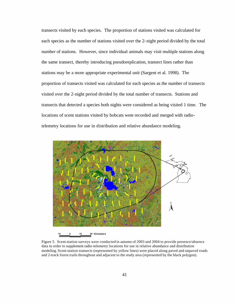
41

transects visited by each species. The proportion of stations visited was calculated for

each species as the number of stations visited over the 2-night period divided by the total

number of stations. However, since individual animals may visit multiple stations along

the same transect, thereby introducing pseudoreplication, transect lines rather than

stations may be a more appropriate experimental unit (Sargent et al. 1998). The

proportion of transects visited was calculated for each species as the number of transects

visited over the 2-night period divided by the total number of transects. Stations and

transects that detected a species both nights were considered as being visited 1 time. The

locations of scent stations visited by bobcats were recorded and merged with radio-

telemetry locations for use in distribution and relative abundance modeling.

Figure 5. Scent-station surveys were conducted in autumn of 2003 and 2004 to provide presence/absence data in order to supplement radio-telemetry locations for use in relative abundance and distribution modeling. Scent-station transects (represented by yellow lines) were placed along paved and unpaved roads and 2-track forest trails throughout and adjacent to the study area (represented by the black polygon).

42

Model Variable Selection

I created a grid of 9,113 non-overlapping hexagons and overlaid it on land-cover

of the NLP (Figure 6). Each hexagon had an area equal to the average MCP core area of

radio-collared adult bobcats.

Figure 6. Hexagon grid overlaid on land-cover of the northern Lower Peninsula, Michigan. Habitat and landscape variables were calculated within each 5.1-km2 hexagon (i.e., equivalent to the size of an average adult bobcat core area) for modeling bobcat distribution and relative abundance.

Within each hexagon, I calculated 139 habitat and landscape variables from 8

metric groups (Table 7) using the Spatial Statistics by Regions interface of the Patch

Analyst Grid 3.0 extension to ArcView GIS 3.2 (Environmental Systems Research

Institute, Redlands, California, USA). I log10-transformed habitat proportions and used a

value of 0.0001 for null proportions (i.e., habitats that were not present within a hexagon)

(Aebischer et al. 1993, Nielsen and Woolf 2002). Habitat proportions were log10-

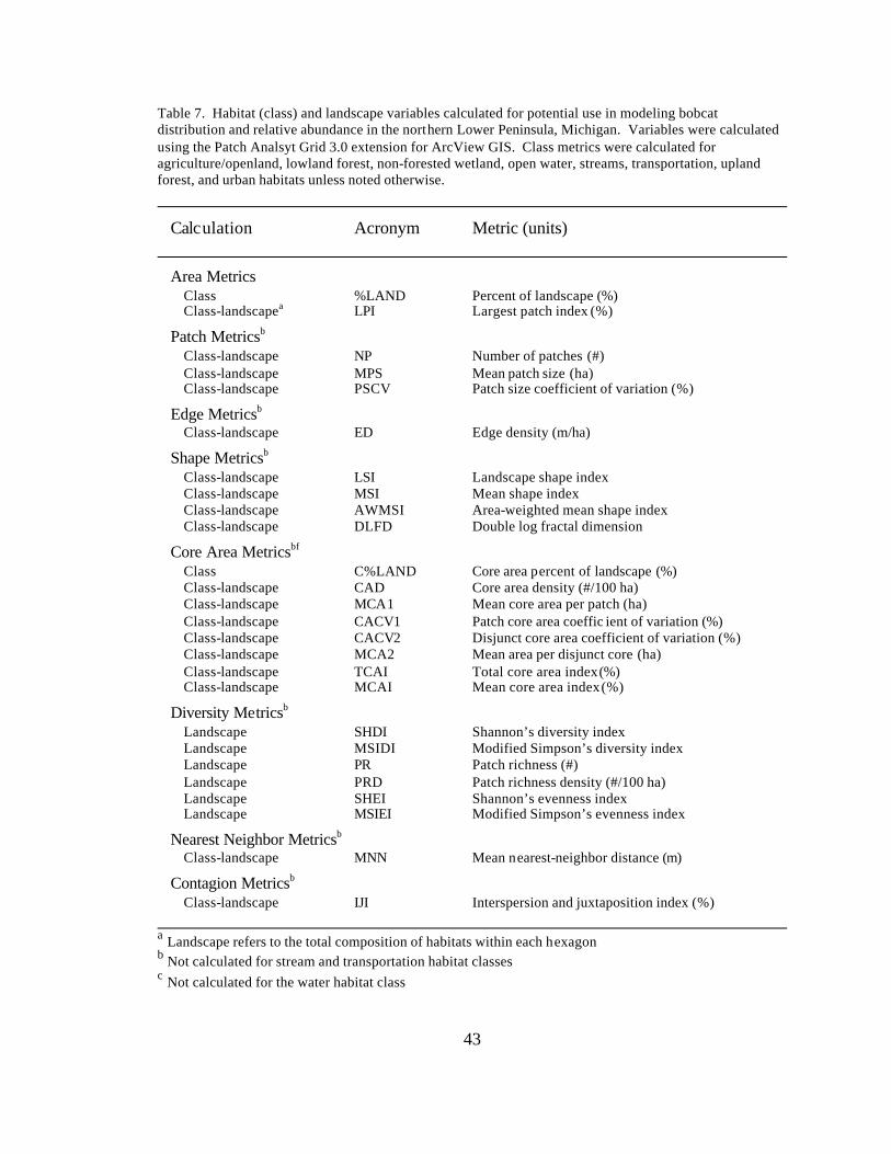
43

Table 7. Habitat (class) and landscape variables calculated for potential use in modeling bobcat distribution and relative abundance in the northern Lower Peninsula, Michigan. Variables were calculated using the Patch Analsyt Grid 3.0 extension for ArcView GIS. Class metrics were calculated for agriculture/openland, lowland forest, non-forested wetland, open water, streams, transportation, upland forest, and urban habitats unless noted otherwise.

Calculation Acronym Metric (units)

Area Metrics Class %LAND Percent of landscape (%) Class-landscapea LPI Largest patch index (%)

Patch Metricsb Class-landscape NP Number of patches (#) Class-landscape MPS Mean patch size (ha) Class-landscape PSCV Patch size coefficient of variation (%)

Edge Metricsb Class-landscape ED Edge density (m/ha)

Shape Metricsb Class-landscape LSI Landscape shape index Class-landscape MSI Mean shape index Class-landscape AWMSI Area-weighted mean shape index Class-landscape DLFD Double log fractal dimension

Core Area Metricsbf Class C%LAND Core area percent of landscape (%) Class-landscape CAD Core area density (#/100 ha) Class-landscape MCA1 Mean core area per patch (ha) Class-landscape CACV1 Patch core area coeffic ient of variation (%) Class-landscape CACV2 Disjunct core area coefficient of variation (%) Class-landscape MCA2 Mean area per disjunct core (ha) Class-landscape TCAI Total core area index (%) Class-landscape MCAI Mean core area index (%)

Diversity Metricsb Landscape SHDI Shannon’s diversity index Landscape MSIDI Modified Simpson’s diversity index Landscape PR Patch richness (#) Landscape PRD Patch richness density (#/100 ha) Landscape SHEI Shannon’s evenness index Landscape MSIEI Modified Simpson’s evenness index

Nearest Neighbor Metricsb Class-landscape MNN Mean nearest-neighbor distance (m)

Contagion Metricsb Class-landscape IJI Interspersion and juxtaposition index (%) a Landscape refers to the total composition of habitats within each hexagon b Not calculated for stream and transportation habitat classes c Not calculated for the water habitat class

44

transformed because they would be more likely to obtain a normal distribution than their

raw values (Aebischer et al. 1993). I reduced the number of variables for analysis based

on the presumed importance of variables to bobcats and univariate statistics. All

statistical analyses (α = 0.05) were performed in SPSS (SPSS, Inc. 1999). I retained a

smaller set of variables for modeling by: 1) retaining the log-transformed proportion of

each habitat class; 2) conducting non-parametric Spearman rank correlations within each

habitat class for variables within each metric group and determining the number of non-

significant correlations per variable; and 3) eliminating 1 of all pairs of correlated

variables within each metric group depending on the number of non-significant

correlations with other variables in the group. I retained variables in each habitat class

most representative of the variables within each metric group. In the case of ties, I

retained the variable suspected to be of greater biological importance to bobcats. This

resulted in 53 potential variables for modeling.

I further reduced the number of potential variables by correlating the variables

within each habitat class. I retained the log10-transformed proportion of each habitat

class, as well as the variable most correlated to others within each habitat class resulting

in 15 potential variables for modeling. Since urban land-cover only occurred in 3 of 11

(27%) core areas of radio-collared bobcats, I excluded the 2 variables associated with

urban land-cover (proportion of urban and edge density of urban). I also excluded the 2

variables associated with open water (proportion of open water and edge density of open

water) because open water only occurred in 4 of 11 (36%) bobcat core areas. This

resulted in 11 variables for use in the final modeling of bobcat distribution and relative

abundance (Table 8). Because further analysis required data normality, I transformed 2

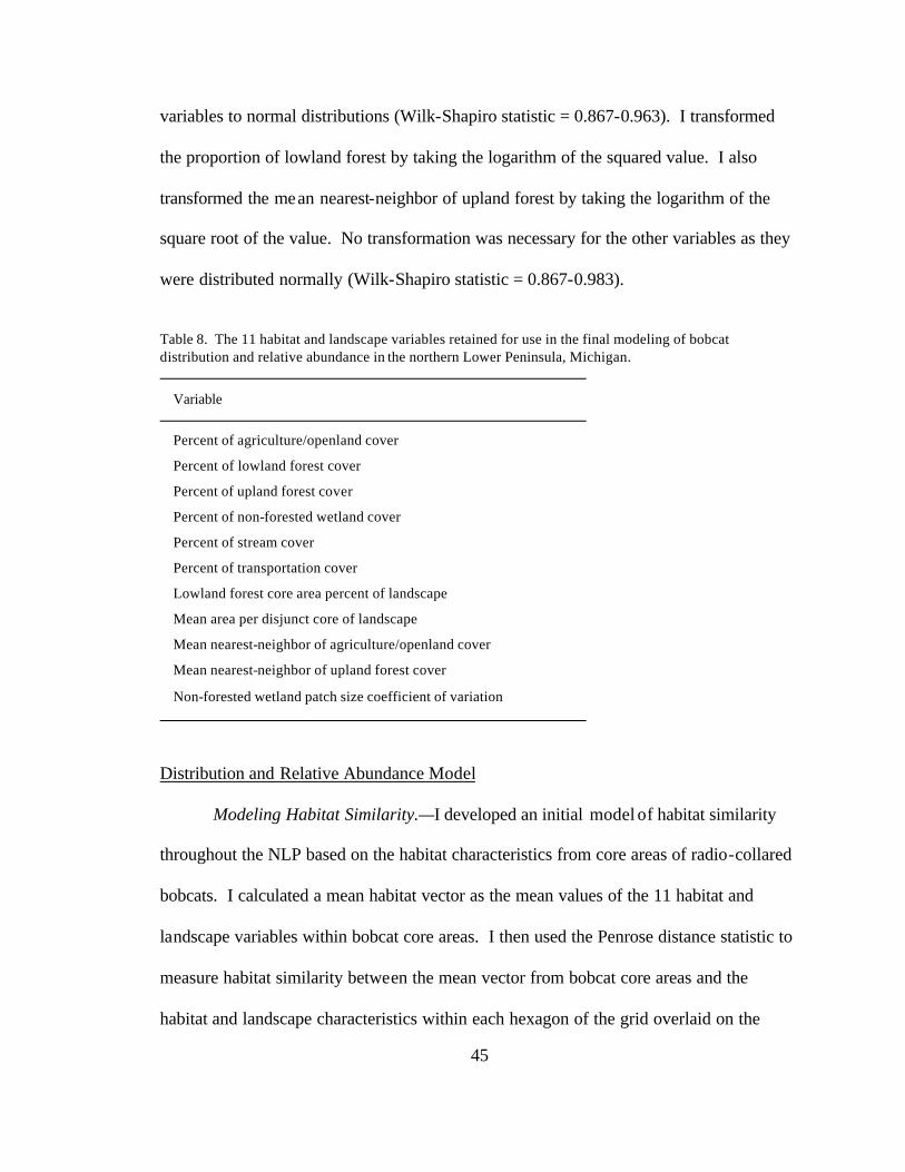
45

variables to normal distributions (Wilk-Shapiro statistic = 0.867-0.963). I transformed

the proportion of lowland forest by taking the logarithm of the squared value. I also

transformed the mean nearest-neighbor of upland forest by taking the logarithm of the

square root of the value. No transformation was necessary for the other variables as they

were distributed normally (Wilk-Shapiro statistic = 0.867-0.983).

Table 8. The 11 habitat and landscape variables retained for use in the final modeling of bobcat distribution and relative abundance in the northern Lower Peninsula, Michigan.

Variable

Percent of agriculture/openland cover

Percent of lowland forest cover

Percent of upland forest cover

Percent of non-forested wetland cover

Percent of stream cover

Percent of transportation cover

Lowland forest core area percent of landscape

Mean area per disjunct core of landscape

Mean nearest-neighbor of agriculture/openland cover

Mean nearest-neighbor of upland forest cover

Non-forested wetland patch size coefficient of variation Distribution and Relative Abundance Model

Modeling Habitat Similarity.—I developed an initial model of habitat similarity

throughout the NLP based on the habitat characteristics from core areas of radio-collared

bobcats. I calculated a mean habitat vector as the mean values of the 11 habitat and

landscape variables within bobcat core areas. I then used the Penrose distance statistic to

measure habitat similarity between the mean vector from bobcat core areas and the

habitat and landscape characteristics within each hexagon of the grid overlaid on the

46

NLP. I calculated Penrose distance as: ; where population i

represented core areas of radio-collared bobcats, population j represented NLP hexagons,

p was the number of habitat variables evaluated, µ was the variable value, k was each

observation, and V was variance (Manly 2005). Habitat composition within each

hexagon of the NLP grid was evaluated relative to the mean habitat vector calculated

from bobcat core areas. The habitat and landscape characteristics of hexagons with

values close to zero were most similar to the characteristics of core areas of radio-

collared bobcats, whereas hexagons with large Penrose distance values had habitat

characteristics less similar to those of bobcat core areas. I made all calculations in a

spreadsheet and appended the final output to the hexagon grid in ArcView GIS to create a

regional map of Penrose distance throughout the NLP. I then correlated Penrose distance

to each habitat variable to determine the relative importance of each variable in

calculating Penrose distance across the NLP.

Modeling Distribution and Relative Abundance.—I developed a spatial model of

the distribution of bobcat relative abundance in the NLP. To model relative abundance, I

associated Penrose distance for each hexagon with abundance information from radio-

collared bobcats and scent-station surveys. I assumed that each hexagon represented 1

bobcat core area. I also assumed that hexagons containing core areas of radio-collared

bobcats represented areas of highest relative abundance (1.0 bobcat per hexagon). I

calculated mean Penrose distance for hexagons containing core areas of radio-collared

bobcats and assumed that all hexagons with a value less than or equal to the mean would

contain 1 bobcat. To determine hexagons with zero relative abundance I overlaid bobcat

locations from radio-telemetry and scent-station surveys on the Penrose distance map. I

( )∑=

−=p

kkkjkiij pVP

1

2 /µµ

47

determined the maximum Penrose distance value for hexagons in which bobcats were

detected and assumed that hexagons with a Penrose distance value greater than that

would contain no bobcats (0 bobcats per hexagon). I estimated intermediate relative

abundance (i.e., values between 0 and 1.0 bobcat per hexagon) by calculating frequency

distributions of the occurrence of bobcat locations in relation to Penrose distance. I

developed a mathematical relationship between the frequency of bobcat locations and

Penrose distance to estimate these intermediate relative abundances. The logarithmic

curve: y = -0.69 ln[x] + 1.5; where x is Penrose distance and y is bobcat abundance,

yielded the greatest R2 value (0.87). I then quantified the area of land predicted to

support 0.51-0.75 and 0.76-1.0 bobcat per hexagon to obtain an estimate of the area of

potential habitat suitable to bobcats.

Model Validation.—I validated the relative abundance model by overlaying an

independent set of locations (n = 196) obtained from harvested bobcats registered with

the MDNR during the 2002 – 2003 bobcat hunting season. I then calculated frequency

distributions of the percentage of harvested bobcats occurring in each density (i.e.,

abundance) class of the relative abundance model.

Results

I captured and radio-collared a total of 15 bobcats (5 females and 10 males).

Thirteen (5 females and 8 males) of the 15 bobcats captured and radio collared were

classified as adults. Two other males were classified as juveniles. I obtained 915

locations on 13 adult bobcats from May 2003 – October 2004. Investigation of plots of

home-range area against number of locations indicated that 11 adult bobcats (5 females

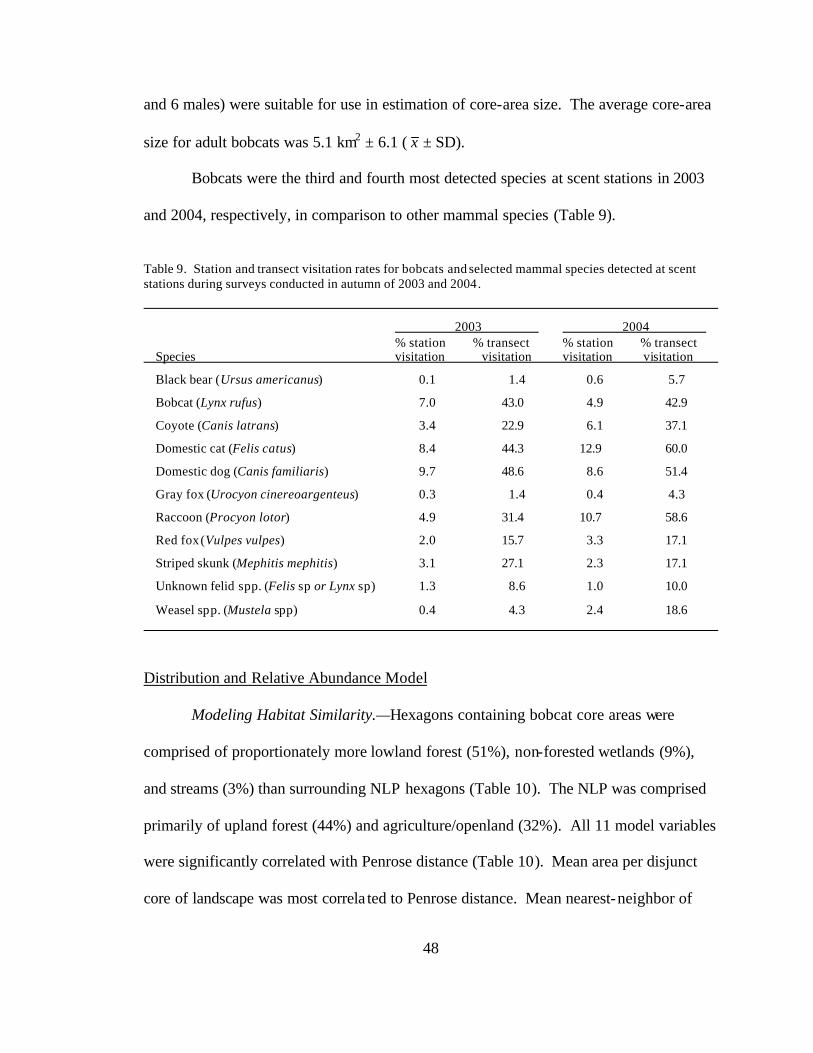
48

and 6 males) were suitable for use in estimation of core-area size. The average core-area

size for adult bobcats was 5.1 km2 ± 6.1 ( x ± SD).

Bobcats were the third and fourth most detected species at scent stations in 2003

and 2004, respectively, in comparison to other mammal species (Table 9).

Table 9. Station and transect visitation rates for bobcats and selected mammal species detected at scent stations during surveys conducted in autumn of 2003 and 2004.

2003 2004 % station % transect % station % transect Species visitation visitation visitation visitation

Black bear (Ursus americanus) 0.1 1.4 0.6 5.7

Bobcat (Lynx rufus) 7.0 43.0 4.9 42.9

Coyote (Canis latrans) 3.4 22.9 6.1 37.1

Domestic cat (Felis catus) 8.4 44.3 12.9 60.0

Domestic dog (Canis familiaris) 9.7 48.6 8.6 51.4

Gray fox (Urocyon cinereoargenteus) 0.3 1.4 0.4 4.3

Raccoon (Procyon lotor) 4.9 31.4 10.7 58.6

Red fox (Vulpes vulpes) 2.0 15.7 3.3 17.1

Striped skunk (Mephitis mephitis) 3.1 27.1 2.3 17.1

Unknown felid spp. (Felis sp or Lynx sp) 1.3 8.6 1.0 10.0

Weasel spp. (Mustela spp) 0.4 4.3 2.4 18.6

Distribution and Relative Abundance Model

Modeling Habitat Similarity.—Hexagons containing bobcat core areas were

comprised of proportionately more lowland forest (51%), non-forested wetlands (9%),

and streams (3%) than surrounding NLP hexagons (Table 10). The NLP was comprised

primarily of upland forest (44%) and agriculture/openland (32%). All 11 model variables

were significantly correlated with Penrose distance (Table 10). Mean area per disjunct

core of landscape was most correla ted to Penrose distance. Mean nearest-neighbor of

49

Table 10. Mean values (± SE) of 11 habitat variables used for modeling distribution and relative abundance of bobcats in the northern Lower Peninsula, Michigan (NLP), and the correlations between each variable and Penrose distance (PD). Values were calculated from 50% minimum convex polygon core areas of 11 radio-collared bobcats (mean vector) and from within hexagons of a hexagon grid overlaid on the NLP. The mean habitat vector was calculated as the mean values of the 11 habitat and landscape variables within bobcat core areas. All correlations between NLP hexagon variables and Penrose distance were significant (P ≤ 0.05). Correlation between NLP Mean NLP hexagons Variablea vector hexagons and PD

Percent of agriculture/openland cover 15.8 ± 2.5 32.4 ± 0.2 -0.471

Percent of lowland forest cover 51.4 ± 5.0 10.4 ± 0.1 0.414

Percent of upland forest cover 17.6 ± 4.1 43.7 ± 0.2 -0.439

Percent of non-forested wetland cover 8.6 ± 1.4 2.3 ± 0.1 -0.438

Percent of stream cover 3.4 ± 0.9 0.9 ± 0.1 -0.223

Percent of transportation cover 3.0 ± 0.5 5.2 ± 0.1 -0.425

Lowland forest core area percent of landscape 27.6 ± 4.5 3.6 ± 0.1 -0.469

Mean area per disjunct core of landscape 0.7 ± 0.1 2.6 ± 0.3 0.922

Mean nearest-neighbor of agriculture/openland cover 50.0 ± 2.5 44.9 ± 0.1 0.259

Mean nearest-neighbor of upland forest cover 55.0 ± 7.6 43.6 ± 0.3 0.061

Non-forested wetland patch size coefficient of variation 208.3 ± 28.5 120.1 ± 0.8 -0.416 a Percent of habitat cover values are presented as raw percents and not their log10-transformed equivalents. upland forest and agriculture/openland cover, as well as proportion of stream cover,

appeared least important in determining Penrose distance across the NLP. Mean Penrose

distance for bobcat core areas was 2.17 ± 1.5 ( x ± SD) and ranged from 0.42 to 7.58.

Mean Penrose distance for NLP hexagons was 3.54 ± 4.1 ( x ± SD) and ranged from 0.12

to 76.79. No locations of bobcats occurred in hexagons with Penrose distance value

>8.45. Throughout the NLP, 1,761 of 9,113 (19%) hexagons had a Penrose distance

≤ 2.17 (Figure 7). Areas with habitat characteristics most similar (i.e., lowest Penrose

distance) to bobcat core areas occurred in the northeast and central parts of the NLP.

Areas with low Penrose distance were characterized primarily by lowland forest and non-

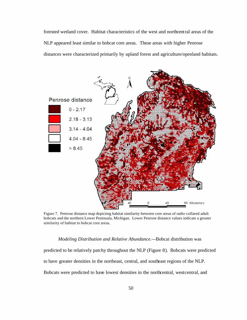
50

forested wetland cover. Habitat characteristics of the west and northcentral areas of the

NLP appeared least similar to bobcat core areas. These areas with higher Penrose

distances were characterized primarily by upland forest and agriculture/openland habitats.

Figure 7. Penrose distance map depicting habitat similarity between core areas of radio-collared adult bobcats and the northern Lower Peninsula, Michigan. Lower Penrose distance values indicate a greater similarity of habitat to bobcat core areas.

Modeling Distribution and Relative Abundance.—Bobcat distribution was

predicted to be relatively patchy throughout the NLP (Figure 8). Bobcats were predicted

to have greater densities in the northeast, central, and southeast regions of the NLP.

Bobcats were predicted to have lowest densities in the northcentral, westcentral, and

51

extreme southeast regions. A total of 36,556 km2 of the NLP (75% of total area) was

predicted to be suitable bobcat habitat. Approximately 16,090 km2 (33% of total area)

and 20,466 km2 (42% of total area) of habitat were predicted to support 0.51-0.75 and

0.76-1.0 bobcat per hexagon, respectively.

Figure 8. Map of the northern Lower Peninsula, Michigan (NLP) depicting predicted relative abundance of bobcats throughout the region. Bobcat abundance is based on a relationship between the similarity of habitat in the NLP to the habitat characteristics of bobcat core areas and abundance information from radio-collared bobcats and scent-station surveys.

Model Validation.—The majority of independent bobcat harvest locations

occurred in areas of the NLP predicted to have greatest bobcat density (Figure 9).

Frequency distributions of harvest locations indicated that 75% of locations occurred in

52

the highest density class (i.e., 0.76-1.0), 19% of locations occurred in the second highest

density class (i.e., 0.51-0.75), and 6% of locations occurred in the lowest density class

(i.e., 0.0-0.50).

Figure 9. Map of bobcat relative abundance in the northern Lower Peninsula, Michigan with locations of 196 bobcats harvested during the 2002 – 2003 Michigan bobcat hunting season. Locations from harvested bobcats were used for model validation. The area south and west of the yellow line is closed to bobcat hunting.

Discussion

Regional models of habitat suitability have been developed for bobcats (Conner et

al. 2001, Lovallo et al. 2001, Nielsen and Woolf 2002), as well as a number of other

carnivore species including black bears (Ursus americanus, Clark et al. 1993), Canada

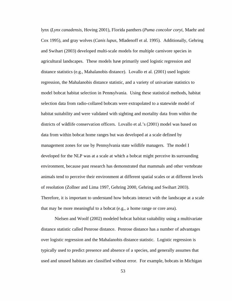
53

lynx (Lynx canadensis, Hoving 2001), Florida panthers (Puma concolor coryi, Maehr and

Cox 1995), and gray wolves (Canis lupus, Mladenoff et al. 1995). Additionally, Gehring

and Swihart (2003) developed multi-scale models for multiple carnivore species in

agricultural landscapes. These models have primarily used logistic regression and

distance statistics (e.g., Mahalanobis distance). Lovallo et al. (2001) used logistic

regression, the Mahalanobis distance statistic, and a variety of univariate statistics to

model bobcat habitat selection in Pennsylvania. Using these statistical methods, habitat

selection data from radio-collared bobcats were extrapolated to a statewide model of

habitat suitability and were validated with sighting and mortality data from within the

districts of wildlife conservation officers. Lovallo et al.’s (2001) model was based on

data from within bobcat home ranges but was developed at a scale defined by

management zones for use by Pennsylvania state wildlife managers. The model I

developed for the NLP was at a scale at which a bobcat might perceive its surrounding

environment, because past research has demonstrated that mammals and other vertebrate

animals tend to perceive their environment at different spatial scales or at different levels

of resolution (Zollner and Lima 1997, Gehring 2000, Gehring and Swihart 2003).

Therefore, it is important to understand how bobcats interact with the landscape at a scale

that may be more meaningful to a bobcat (e.g., a home range or core area).

Nielsen and Woolf (2002) modeled bobcat habitat suitability using a multivariate

distance statistic called Penrose distance. Penrose distance has a number of advantages

over logistic regression and the Mahalanobis distance statistic. Logistic regression is

typically used to predict presence and absence of a species, and generally assumes that

used and unused habitats are classified without error. For example, bobcats in Michigan

54

primarily use lowland conifer forest (Section 1), however, aspen clear-cuts may be an

important habitat for procuring prey. If sampling methods (e.g., radio-telemetry, scent-

station surveys) for determining bobcat habitat use did not detect bobcats in aspen clear-

cuts, logistic regression models would predict bobcats to be absent from that habitat

when, in fact, they did occur there (Type I error). Penrose distance does not require the

assumption that used and unused habitats are classified without error. The Mahalanobis

distance statistic has been shown to provide similar results to Penrose distance (Manly

2005), however there are several differences between these 2 methods. Mahalanobis

distance accounts for correlations between variables which Penrose distance does not. In

my analysis, I conducted correlation analysis to remove correlated variables before

employing the Penrose distance statistic. The Mahalanobis distance equation, however,

does not contain squared terms (Manly 2005), which precluded its use in my analysis

because the log10-transformed habitat proportions were often negative.

The model I developed was based on the method implemented in southern Illinois

involving the use of data from radio-collared bobcats, remotely-sensed land-cover, and

the Penrose distance statistic to develop a habitat-relative abundance relationship for an

unharvested bobcat population (Nielsen and Woolf 2002). Nielsen and Woolf (2002)

developed this model for use by wildlife managers in Illinois where bobcats had been

listed as state threatened until 1999. Similarly, I used data from radio-collared bobcats,

remotely-sensed land-cover, and the Penrose distance statistic to model distribution and

relative abundance throughout the NLP for a harvested bobcat population. Because

radio-telemetry data were collected from relatively few (n = 11) bobcats, I conducted

scent-station surveys to supplement telemetry data. Scent-station surveys have been

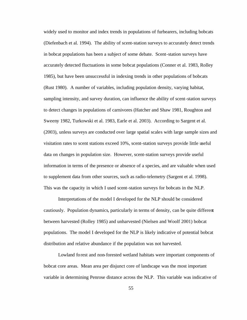
55

widely used to monitor and index trends in populations of furbearers, including bobcats

(Diefenbach et al. 1994). The ability of scent-station surveys to accurately detect trends

in bobcat populations has been a subject of some debate. Scent-station surveys have

accurately detected fluctuations in some bobcat populations (Conner et al. 1983, Rolley

1985), but have been unsuccessful in indexing trends in other populations of bobcats

(Rust 1980). A number of variables, including population density, varying habitat,

sampling intensity, and survey duration, can influence the ability of scent-station surveys

to detect changes in populations of carnivores (Hatcher and Shaw 1981, Roughton and

Sweeny 1982, Turkowski et al. 1983, Earle et al. 2003). According to Sargent et al.

(2003), unless surveys are conducted over large spatial scales with large sample sizes and

visitation rates to scent stations exceed 10%, scent-station surveys provide little useful

data on changes in population size. However, scent-station surveys provide useful

information in terms of the presence or absence of a species, and are valuable when used

to supplement data from other sources, such as radio-telemetry (Sargent et al. 1998).

This was the capacity in which I used scent-station surveys for bobcats in the NLP.

Interpretations of the model I developed for the NLP should be considered

cautiously. Population dynamics, particularly in terms of density, can be quite different

between harvested (Rolley 1985) and unharvested (Nielsen and Woolf 2001) bobcat

populations. The model I developed for the NLP is likely indicative of potential bobcat

distribution and relative abundance if the population was not harvested.

Lowland forest and non-forested wetland habitats were important components of

bobcat core areas. Mean area per disjunct core of landscape was the most important

variable in determining Penrose distance across the NLP. This variable was indicative of

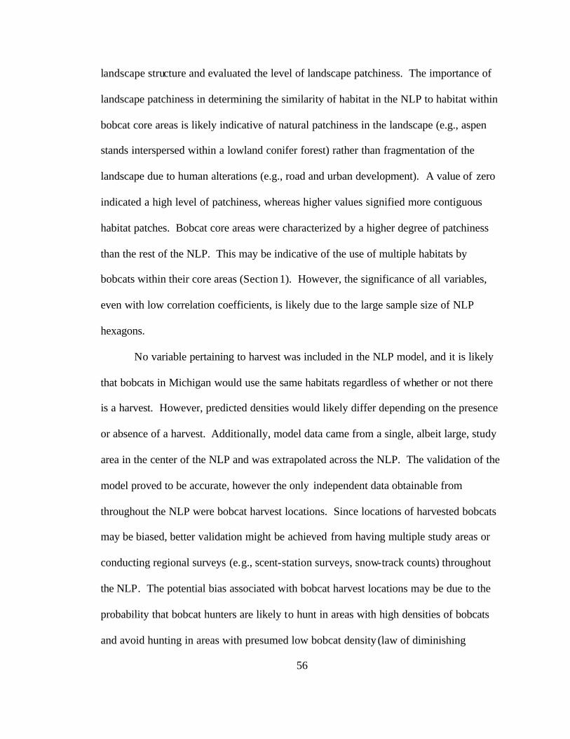
56

landscape structure and evaluated the level of landscape patchiness. The importance of

landscape patchiness in determining the similarity of habitat in the NLP to habitat within

bobcat core areas is likely indicative of natural patchiness in the landscape (e.g., aspen

stands interspersed within a lowland conifer forest) rather than fragmentation of the

landscape due to human alterations (e.g., road and urban development). A value of zero

indicated a high level of patchiness, whereas higher values signified more contiguous

habitat patches. Bobcat core areas were characterized by a higher degree of patchiness

than the rest of the NLP. This may be indicative of the use of multiple habitats by

bobcats within their core areas (Section 1). However, the significance of all variables,

even with low correlation coefficients, is likely due to the large sample size of NLP

hexagons.

No variable pertaining to harvest was included in the NLP model, and it is likely

that bobcats in Michigan would use the same habitats regardless of whether or not there

is a harvest. However, predicted densities would likely differ depending on the presence

or absence of a harvest. Additionally, model data came from a single, albeit large, study

area in the center of the NLP and was extrapolated across the NLP. The validation of the

model proved to be accurate, however the only independent data obtainable from

throughout the NLP were bobcat harvest locations. Since locations of harvested bobcats

may be biased, better validation might be achieved from having multiple study areas or

conducting regional surveys (e.g., scent-station surveys, snow-track counts) throughout

the NLP. The potential bias associated with bobcat harvest locations may be due to the

probability that bobcat hunters are likely to hunt in areas with high densities of bobcats

and avoid hunting in areas with presumed low bobcat density (law of diminishing

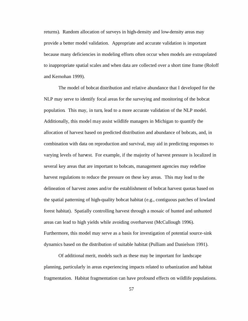
57

returns). Random allocation of surveys in high-density and low-density areas may

provide a better model validation. Appropriate and accurate validation is important

because many deficiencies in modeling efforts often occur when models are extrapolated

to inappropriate spatial scales and when data are collected over a short time frame (Roloff

and Kernohan 1999).

The model of bobcat distribution and relative abundance that I developed for the

NLP may serve to identify focal areas for the surveying and monitoring of the bobcat

population. This may, in turn, lead to a more accurate validation of the NLP model.

Additionally, this model may assist wildlife managers in Michigan to quantify the

allocation of harvest based on predicted distribution and abundance of bobcats, and, in

combination with data on reproduction and survival, may aid in predicting responses to

varying levels of harvest. For example, if the majority of harvest pressure is localized in

several key areas that are important to bobcats, management agencies may redefine

harvest regulations to reduce the pressure on these key areas. This may lead to the

delineation of harvest zones and/or the establishment of bobcat harvest quotas based on

the spatial patterning of high-quality bobcat habitat (e.g., contiguous patches of lowland

forest habitat). Spatially controlling harvest through a mosaic of hunted and unhunted

areas can lead to high yields while avoiding overharvest (McCullough 1996).

Furthermore, this model may serve as a basis for investigation of potential source-sink

dynamics based on the distribution of suitable habitat (Pulliam and Danielson 1991).

Of additional merit, models such as these may be important for landscape

planning, particularly in areas experiencing impacts related to urbanization and habitat

fragmentation. Habitat fragmentation can have profound effects on wildlife populations.

58

Bobcats have been shown to be sensitive to levels of habitat fragmentation (Crooks

2002). In particular, fragmentation of habitat can reduce the abundance and distribution

of wildlife populations (Saunders et al. 1991), including species of mammalian predators

(Gehring 2000, Gehring and Swihart 2003). A specific concern relating to habitat

fragmentation is that mammals such as wolves and bobcats may be exposed to increased

human induced mortality (Mladenoff et al. 1995). Saunders et al. (2002) suggested that

road development has contributed to habitat fragmentation in the Great Lakes Region

more than urban expansion, rural home development, or other types of land use

conversion. Additionally, in areas experiencing habitat fragmentation, carnivores with

large home ranges may be more likely to face declines in population size, or possible

extinction, than those with smaller home ranges, regardless of population density

(Woodroffe and Ginsberg 1998). The NLP is experiencing substantial loss and

fragmentation of habitat, and landscape level species planning would benefit from the

development of a regional conservation plan. Mammalian carnivores are good candidates

for focal species in conservation planning because their patterns of distribution are often

indicative of population processes at a regional scale (Carroll et al. 2001, Gittleman et al.

2001, Noss 2001). With the recent discovery of gray wolves in the NLP, it is becoming

important to consider the needs of several carnivore species and to institute management

efforts at the landscape level. The development of spatial models of distribution and

relative abundance for multiple carnivore species may aid in the delineation of critical

areas needed to promote carnivore conservation within the NLP.

59

LITERATURE CITED

Aebischer, N. J., P. A. Robertson, and R. E. Kenward. 1993. Compositional analysis of

habitat use from animal radio-tracking data. Ecology 74:1313-1325.

Benson, J. F., M. J. Chamberlain, and B. D. Leopold. 2004. Land tenure and occupation

of vacant home ranges by bobcats (Lynx rufus). Journal of Mammalogy 85:983-

988.

Carroll, C., R. F. Noss, and P. C. Paquet. 2001. Carnivores as focal species for

conservation planning in the Rocky Mountain region. Ecological Applications

11:961-980.

Chamberlain, M. J., and B. D. Leopold. 2001. Spatio-temporal relationships among

adult bobcats in central Mississippi. Pages 45-50 in A. Woolf, C. K. Nielsen, and

R. D. Bluett, editors. Proceedings of a symposium on current bobcat research and


Tennessee, USA.

Clark, J. D., J. E. Dunn, and K. G. Smith. 1993. A multivariate model of female black

bear habitat use for a GIS. Journal of Wildlife Management 57:519-526.



3400.

60

Conner, L. M., B. D. Leopold, and M. J. Chamberlain. 2001. Multivariate habitat

models for bobcats in southern forested landscapes. Pages 51-55 in A. Woolf, C.

K. Nielsen, and R. D. Bluett, editors. Proceedings of a symposium on current

bobcat research and implications for management. The Wildlife Society 2000

Conference, Nashville, Tennessee, USA.

Conner, M. C., R. F. Labisky, and D. R. Progulske. 1983. Scent-station indices as

measures of population abundance for bobcats, raccoons, gray foxes, and

opossums. Wildlife Society Bulletin 11:146-152.

Crooks, K. R. 2002. Relative sensitivities of mammalian carnivores to habitat

fragmentation. Conservation Biology 16:488-502.

Diefenbach, D. R., M. J. Conroy, R. J. Warren, W. E. James, L. A. Baker, and T. Hon.

1994. A test of the scent-station survey technique for bobcats. Journal of

Wildlife Management 58:10-17.

Dixon, K. R., and J. A. Chapman. 1980. Harmonic mean measure of animal activity

areas. Ecology 61:1040-1044.



Earle, R. D. , D. R. Etter, S. L. Mayhew, and V. R. Tuovila. 2003. Bobcat population

survey methods. Michigan Department of Natural Resources. Study No. 147-

108.

Frawley, B. J., D. Etter, and D. Bostick. 2004. Bobcat hunter and trapper opinion

survey. Michigan Department of Natural Resources. Wildlife Report No. 3427.

61

Fritts, S. H., and J. A. Sealander. 1978. Reproductive biology and population

characteristics of bobcats (Lynx rufus) in Arkansas. Journal of Mammalogy

59:347-353.

Gehring, T. M. 2000. Ecology of mammalian predators in a landscape fragmented by

agriculture. Ph.D. Dissertation, Purdue University, West Lafayette, Indiana,

USA.

Gehring, T. M., and R. K. Swihart. 2003. Body size, niche breadth, and ecologically

scaled responses to habitat fragmentation: mammalian predators in an

agricultural landscape. Biological Conservation 109:283-295.

Gittleman, J. L., S. M. Funk, D. Mcdonald, and R. K. Wayne. 2001. Carnivore

conservation. Cambridge University Press, Cambridge, United Kingdom.

Hatcher, R. T., and J. H. Shaw. 1981. A comparison of 3 indices to furbearer

populations. Wildlife Society Bulletin 9:153-156.

Hoving, C. L. 2001. Historical occurrence and habitat ecology of Canada lynx (Lynx

canadensis) in eastern North America. M.S. Thesis, University of Maine, Orono,

Maine, USA.

Kenward, R. E. 2001. A manual for wildlife radio tagging. Academic Press, San Diego,

California, USA.

Lancia, R. A., J. D. Nichols, and K. H. Pollock. 1996. Estimating the number of animals

in wildlife populations. Pages 215-253 in T. A. Bookhout, editor. Research and

management techniques for wildlife and habitats. Fifth edition, revised. The

Wildlife Society, Bethesda, Maryland, USA.

62

Leatherberry, E. C. 1994. Forest statistics for Michigan’s Northern Lower Peninsula

Unit, 1993. United States Department of Agriculture, Forest Service, North

Central Forest Experiment Station, Saint Paul, Minnesota. Resource Bulletin NC

157.

Linhart, S. B., and F. F. Knowlton. 1975. Determining the relative abundance of coyotes

by scent station lines. Wildlife Society Bulletin 3:119-124.

Lovallo, M. J., G. L. Storm, D. S. Klute, and W. M. Tzilkowski. 2001. Multivariate

models of bobcat habitat selection for Pennsylvania landscapes. Pages 4-17 in

A.Woolf, C. K. Nielsen, and R. D. Bluett, editors. Proceedings of a symposium

on current bobcat research and implications for management. The Wildlife

Society 2000 Conference, Nashville, Tennessee, USA.

Maehr, D. S., and J. A. Cox. 1995. Landscape features and panthers in Florida.

Conservation Biology 9:1008-1019.

Manly, B. F. J. 2005. Multivariate statistical methods: a primer. Third edition.

Chapman and Hall/CRC Press, Boca Raton, Florida, USA.

McCullough, D. R. 1996. Spatially structured populations and harvest theory. Journal


Mladenoff, D. J., T. A. Sickley, R. G. Haight, and A. P. Wydeven. 1995. A regional

landscape analysis prediction of favorable gray wolf habitat in the northern Great

Lakes region. Conservation Biology 9:279-294.

Mohr, C. O. 1947. Table of equivalent populations of North American small mammals.

American Midland Naturalist 37:233-249.

63

Murie, O. J. 1974. The Peterson field guide series: a field guide to animal tracks.

Houghton Mifflin Company, New York, New York, USA.

Nielsen, C. K., and A. Woolf. 2001. Spatial organization of bobcats (Lynx rufus) in

southern Illinois. American Midland Naturalist 146:43-52.

Nielsen, C. K., and A. Woolf. 2002. Habitat-relative abundance relationship for bobcats

in southern Illinois. Wildlife Society Bulletin 30:222-230.

Noss, R. F. 2001. Introduction: why restore large mammals? Pages 1-21 in D. S.

Maehr, R. F. Noss, and J. L. Larkin, editors. Large mammal restoration:

ecological and sociological challenges in the 21st century. Island Press,

Washington, D.C., USA.

Powell, R. A. 2000. Animal home ranges and territories and home range estimators.

Pages 65-110 in L. Boitani, and T. K. Fuller, editors. Research techniques in

animal ecology: controversies and consequences. Columbia University Press,


Pulliam, H. R., and B. J. Danielson. 1991. Sources, sinks, and habitat selection: a

landscape perspective on population dynamics. American Naturalist 137:S50-

S66.

Rodgers, A. R., and A. P. Carr. 1998. HRE: the home range extension for Arcview.

Version 0.9. Centre for Northern Forest Ecosystem Research, Ontario Ministry of

Natural Resources, Canada.

Rolley, R. E. 1985. Dynamics of a harvested bobcat population in Oklahoma. Journal


64

Rolley, R. E., B. E. Kohn, and J. F. Olson. 2001. Evolution of Wisconsin's bobcat

harvest management program. Pages 61-66 in A.Woolf, C. K. Nielsen, and R. D.

Bluett, editors. Proceedings of a symposium on current bobcat research and


Tennessee, USA.

Roloff, G. J., and B. J. Kernohan. 1999. Evaluating reliability of habitat suitability index

models. Wildlife Society Bulletin 27:973-985.

Roughton, R. D., and M. W. Sweeny. 1982. Refinements in scent-station methodology

for assessing trends in carnivore populations. Journal of Wildlife Management

46:217-229.

Rust, W. D. 1980. Scent station transects as a means of indexing bobcat population

fluctuations. M.S. Thesis, Tennessee Technological University, Cookeville,

Tennessee, USA.

Samuel, M. D., D. J. Pierce, and E. O. Garton. 1985. Identifying areas of concentrated

use within the home range. Journal of Animal Ecology 54:711-719.

Sargent, G. A., D. H. Johnson, and W. E. Berg. 1998. Interpreting carnivore scent-

station surveys. Journal of Wildlife Management 62:1235-1245.

Sargent, G. A., D. H. Johnson, and W. E. Berg. 2003. Sampling designs for carnivore

scent-station surveys. Journal of Wildlife Management 67:289-298.

Saunders, D. A., R. J. Hobbs, and C. R. Margules. 1991. Biological consequences of

ecosystem fragmentation: a review. Conservation Biology 5:18-32.

65

Saunders, D. A., M. R. Mislivets, J. Chen, and D. T. Cleland. 2002. Effects of roads on

landscape structure within nested ecological units of the northern Great Lakes

Region, USA. Biological Conservation 103:209-225.

Seaman, D. E., J. J. Millspaugh, B. J. Kernohan, G. C. Brundige, K. J. Raedeke, and R.

A. Gitzen. 1999. Effects of sample size on kernel home range estimates. Journal


Thornton, D. H., M. E. Sunquist, and M. B. Main. 2004. Ecological separation within

newly sympatric populations of coyotes and bobcats in south-central Florida.

Journal of Mammalogy 85:973-982.

Turkowski, F. J., M. L. Popelka, and R. W. Bullard. 1983. Efficacy of odor lures and

baits for coyotes. Wildlife Society Bulletin 11:136-145.

Whitaker, J. O., Jr. 1996. National Audubon Society field guide to North American

mammals. Alfred A. Knopf, Inc., New York, New York, USA.

Woodroffe, R., and J. R. Ginsberg. 1998. Edge effects and the extinction of populations

inside protected areas. Science 280:2126-2128.

Woolf, A., C.K. Nielsen, T. Weber, and T. J. Gibbs-Kieninger. 2002. Statewide

modeling of bobcat, Lynx rufus, habitat in Illinois, USA. Biological Conservation

104:191-198.

Zollner, P. A., and S. L. Lima. 1997. Landscape-level perceptual abilities in white-

footed mice: perceptual range and the detection of forested habitat. Oikos 80:51-

60.

Documents

Copy of Preuss MS thesis final - people.se.cmich.edu