8/9/2019 Copy of Additional Mathematics Project 2010

http://slidepdf.com/reader/full/copy-of-additional-mathematics-project-2010 1/14

PROJECT WORK FOR ADDITIONAL

MATHEMATICS 2010

Probability in Our Life

NAMA : MOHD HAMIZAN BIN MOHD ALI

GURU PEMBIMBING : MR. CH'NG YEANG SOON

I/C : 930110-02-5243

SEKOLAH : PENANG FREE SCHOOL

8/9/2019 Copy of Additional Mathematics Project 2010

http://slidepdf.com/reader/full/copy-of-additional-mathematics-project-2010 2/14

CONTENT

 No Contents Page

1 Introduction

2 Part 1

3 Part 2

4 Part 3

5 Part 4

6 Part 5

7 Conclusion

8/9/2019 Copy of Additional Mathematics Project 2010

http://slidepdf.com/reader/full/copy-of-additional-mathematics-project-2010 3/14

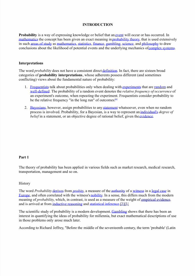
INTRODUCTION

Probability is a way of expressing knowledge or belief that an event will occur or has occurred. In

mathematics the concept has been given an exact meaning in probability theory, that is used extensively

in such areas of study as mathematics, statistics, finance, gambling, science, and philosophy to draw

conclusions about the likelihood of potential events and the underlying mechanics of  complex systems.

Interpretations

The word probability does not have a consistent direct definition. In fact, there are sixteen broadcategories of probability interpretations, whose adherents possess different (and sometimes

conflicting) views about the fundamental nature of probability:

1. Frequentists talk about probabilities only when dealing with experiments that are random and

well-defined. The probability of a random event denotes the relative frequency of occurrence of 

an experiment's outcome, when repeating the experiment. Frequentists consider probability to be the relative frequency "in the long run" of outcomes.[1]

2. Bayesians, however, assign probabilities to any statement whatsoever, even when no random

 process is involved. Probability, for a Bayesian, is a way to represent an individual's degree of 

belief in a statement, or an objective degree of rational belief, given the evidence.

Part 1

The theory of probability has been applied in various fields such as market research, medical research,transportation, management and so on.

History

The word Probability derives from probity, a measure of the authority of a witness in a legal case in

Europe, and often correlated with the witness's nobility. In a sense, this differs much from the modernmeaning of  probability, which, in contrast, is used as a measure of the weight of  empirical evidence,

and is arrived at from inductive reasoning and statistical inference.[2] [3]

The scientific study of probability is a modern development. Gambling shows that there has been aninterest in quantifying the ideas of probability for millennia, but exact mathematical descriptions of use

in those problems only arose much later.

According to Richard Jeffrey, "Before the middle of the seventeenth century, the term 'probable' (Latin

8/9/2019 Copy of Additional Mathematics Project 2010

http://slidepdf.com/reader/full/copy-of-additional-mathematics-project-2010 4/14

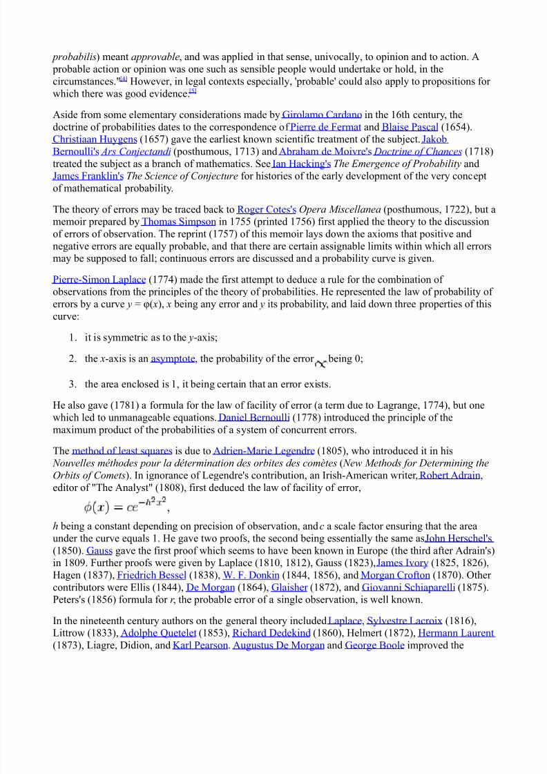
 probabilis) meant approvable, and was applied in that sense, univocally, to opinion and to action. A

 probable action or opinion was one such as sensible people would undertake or hold, in the

circumstances."[4] However, in legal contexts especially, 'probable' could also apply to propositions for 

which there was good evidence.[5]

Aside from some elementary considerations made by Girolamo Cardano in the 16th century, the

doctrine of probabilities dates to the correspondence of Pierre de Fermat and Blaise Pascal (1654).

Christiaan Huygens (1657) gave the earliest known scientific treatment of the subject. JakobBernoulli's  Ars Conjectandi (posthumous, 1713) and Abraham de Moivre's  Doctrine of Chances (1718)

treated the subject as a branch of mathematics. See Ian Hacking's The Emergence of Probability andJames Franklin's The Science of Conjecture for histories of the early development of the very concept

of mathematical probability.

The theory of errors may be traced back to Roger Cotes's Opera Miscellanea (posthumous, 1722), but amemoir prepared by Thomas Simpson in 1755 (printed 1756) first applied the theory to the discussion

of errors of observation. The reprint (1757) of this memoir lays down the axioms that positive and

negative errors are equally probable, and that there are certain assignable limits within which all errorsmay be supposed to fall; continuous errors are discussed and a probability curve is given.

Pierre-Simon Laplace (1774) made the first attempt to deduce a rule for the combination of observations from the principles of the theory of probabilities. He represented the law of probability of 

errors by a curve y = φ( x), x being any error and y its probability, and laid down three properties of this

curve:

1. it is symmetric as to the y-axis;

2. the x-axis is an asymptote, the probability of the error being 0;

3. the area enclosed is 1, it being certain that an error exists.

He also gave (1781) a formula for the law of facility of error (a term due to Lagrange, 1774), but onewhich led to unmanageable equations. Daniel Bernoulli (1778) introduced the principle of the

maximum product of the probabilities of a system of concurrent errors.

The method of least squares is due to Adrien-Marie Legendre (1805), who introduced it in his Nouvelles méthodes pour la détermination des orbites des comètes ( New Methods for Determining the

Orbits of Comets). In ignorance of Legendre's contribution, an Irish-American writer, Robert Adrain,

editor of "The Analyst" (1808), first deduced the law of facility of error,

h being a constant depending on precision of observation, and c a scale factor ensuring that the area

under the curve equals 1. He gave two proofs, the second being essentially the same as John Herschel's(1850). Gauss gave the first proof which seems to have been known in Europe (the third after Adrain's)in 1809. Further proofs were given by Laplace (1810, 1812), Gauss (1823), James Ivory (1825, 1826),

Hagen (1837), Friedrich Bessel (1838), W. F. Donkin (1844, 1856), and Morgan Crofton (1870). Other 

contributors were Ellis (1844), De Morgan (1864), Glaisher (1872), and Giovanni Schiaparelli (1875).Peters's (1856) formula for r , the probable error of a single observation, is well known.

In the nineteenth century authors on the general theory included Laplace, Sylvestre Lacroix (1816),Littrow (1833), Adolphe Quetelet (1853), Richard Dedekind (1860), Helmert (1872), Hermann Laurent 

(1873), Liagre, Didion, and Karl Pearson. Augustus De Morgan and George Boole improved the

8/9/2019 Copy of Additional Mathematics Project 2010

http://slidepdf.com/reader/full/copy-of-additional-mathematics-project-2010 5/14

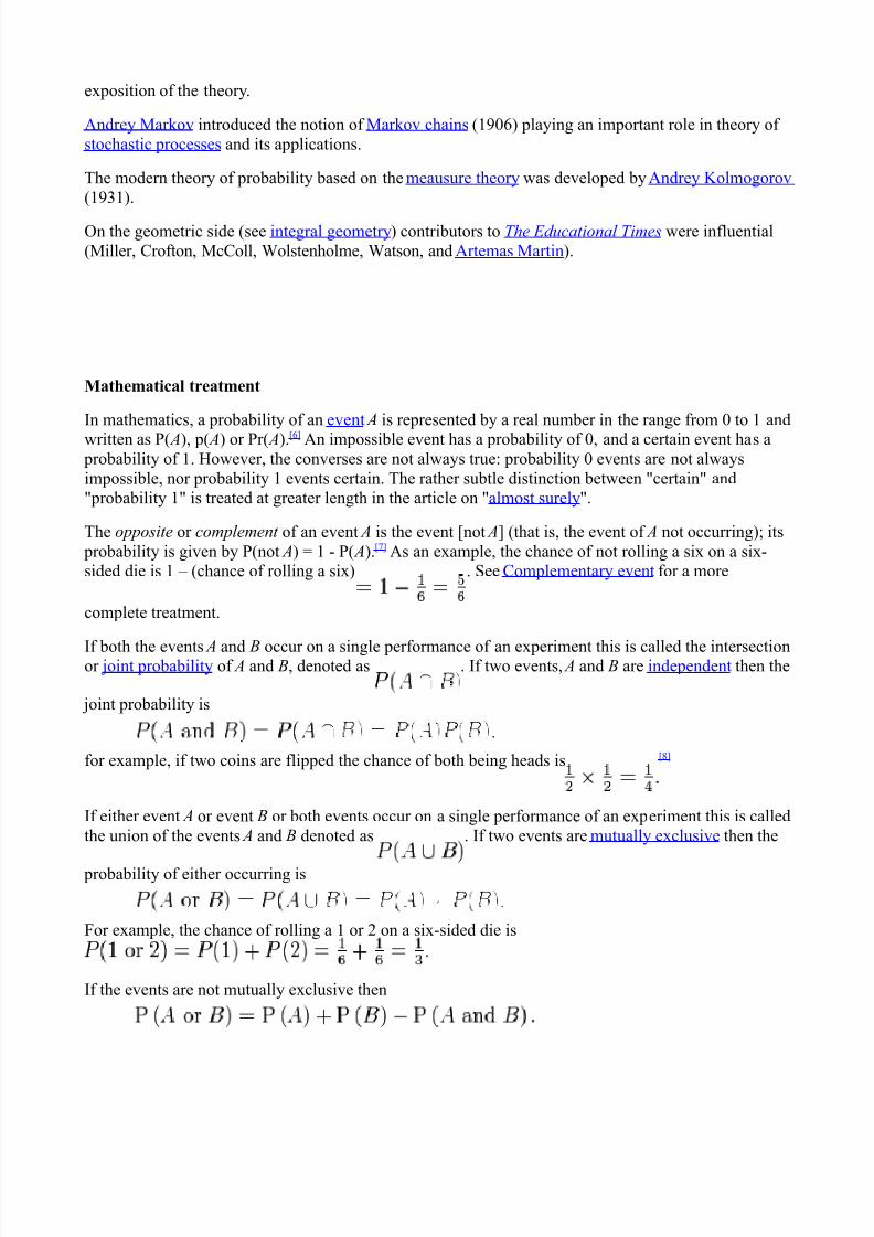
exposition of the theory.

Andrey Markov introduced the notion of Markov chains (1906) playing an important role in theory of 

stochastic processes and its applications.

The modern theory of probability based on the meausure theory was developed by Andrey Kolmogorov 

(1931).

On the geometric side (see integral geometry) contributors to The Educational Times were influential

(Miller, Crofton, McColl, Wolstenholme, Watson, and Artemas Martin).

Mathematical treatment

In mathematics, a probability of an event  A is represented by a real number in the range from 0 to 1 and

written as P( A), p( A) or Pr( A).[6] An impossible event has a probability of 0, and a certain event has a probability of 1. However, the converses are not always true: probability 0 events are not always

impossible, nor probability 1 events certain. The rather subtle distinction between "certain" and"probability 1" is treated at greater length in the article on "almost surely".

The opposite or complement of an event A is the event [not A] (that is, the event of  A not occurring); its

 probability is given by P(not A) = 1 - P( A).[7] As an example, the chance of not rolling a six on a six-sided die is 1 – (chance of rolling a six) . See Complementary event for a more

complete treatment.

If both the events A and B occur on a single performance of an experiment this is called the intersectionor  joint probability of  A and B, denoted as . If two events, A and B are independent then the

 joint probability is

for example, if two coins are flipped the chance of both being heads is [8]

If either event A or event B or both events occur on a single performance of an experiment this is called

the union of the events A and B denoted as . If two events are mutually exclusive then the

 probability of either occurring is

For example, the chance of rolling a 1 or 2 on a six-sided die is

If the events are not mutually exclusive then

8/9/2019 Copy of Additional Mathematics Project 2010

http://slidepdf.com/reader/full/copy-of-additional-mathematics-project-2010 6/14

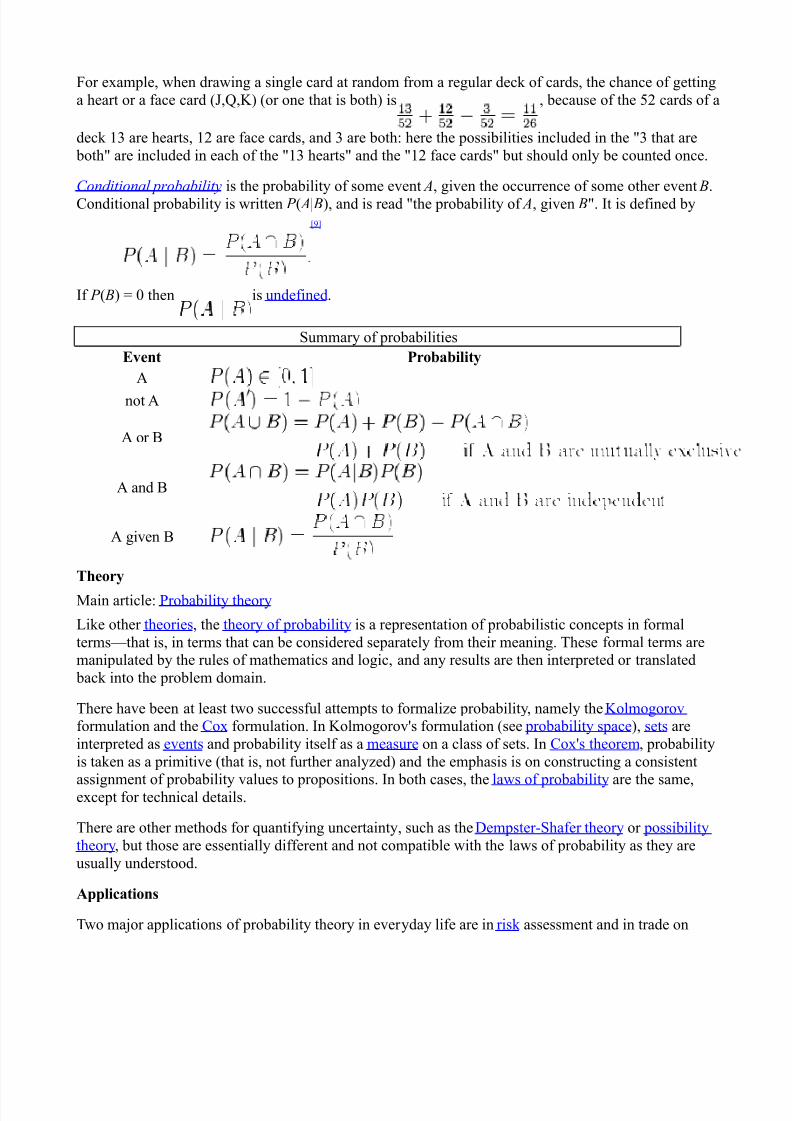
For example, when drawing a single card at random from a regular deck of cards, the chance of getting

a heart or a face card (J,Q,K) (or one that is both) is , because of the 52 cards of a

deck 13 are hearts, 12 are face cards, and 3 are both: here the possibilities included in the "3 that are

 both" are included in each of the "13 hearts" and the "12 face cards" but should only be counted once.

Conditional probability is the probability of some event A, given the occurrence of some other event B.

Conditional probability is written P ( A| B), and is read "the probability of  A, given B". It is defined by

[9]

If  P ( B) = 0 then is undefined.

Summary of probabilities

Event Probability

A

not A

A or B

A and B

A given B

Theory

Main article: Probability theory

Like other theories, the theory of probability is a representation of probabilistic concepts in formal

terms—that is, in terms that can be considered separately from their meaning. These formal terms aremanipulated by the rules of mathematics and logic, and any results are then interpreted or translated

 back into the problem domain.

There have been at least two successful attempts to formalize probability, namely the Kolmogorov formulation and the Cox formulation. In Kolmogorov's formulation (see probability space), sets are

interpreted as events and probability itself as a measure on a class of sets. In Cox's theorem, probability

is taken as a primitive (that is, not further analyzed) and the emphasis is on constructing a consistent

assignment of probability values to propositions. In both cases, the laws of probability are the same,except for technical details.

There are other methods for quantifying uncertainty, such as the Dempster-Shafer theory or  possibility

theory, but those are essentially different and not compatible with the laws of probability as they are

usually understood.

Applications

Two major applications of probability theory in everyday life are in risk assessment and in trade on

8/9/2019 Copy of Additional Mathematics Project 2010

http://slidepdf.com/reader/full/copy-of-additional-mathematics-project-2010 7/14

commodity markets. Governments typically apply probabilistic methods in environmental regulation 

where it is called " pathway analysis", often measuring well-being using methods that are stochastic in

nature, and choosing projects to undertake based on statistical analyses of their probable effect on the

 population as a whole.

A good example is the effect of the perceived probability of any widespread Middle East conflict on oil

 prices - which have ripple effects in the economy as a whole. An assessment by a commodity trader 

that a war is more likely vs. less likely sends prices up or down, and signals other traders of thatopinion. Accordingly, the probabilities are not assessed independently nor necessarily very rationally.

The theory of  behavioral finance emerged to describe the effect of such groupthink on pricing, on policy, and on peace and conflict.

It can reasonably be said that the discovery of rigorous methods to assess and combine probability

assessments has had a profound effect on modern society. Accordingly, it may be of some importanceto most citizens to understand how odds and probability assessments are made, and how they contribute

to reputations and to decisions, especially in a democracy.

Another significant application of probability theory in everyday life is reliability. Many consumer 

 products, such as automobiles and consumer electronics, utilize reliability theory in the design of the product in order to reduce the probability of failure. The probability of failure may be closelyassociated with the product's warranty.

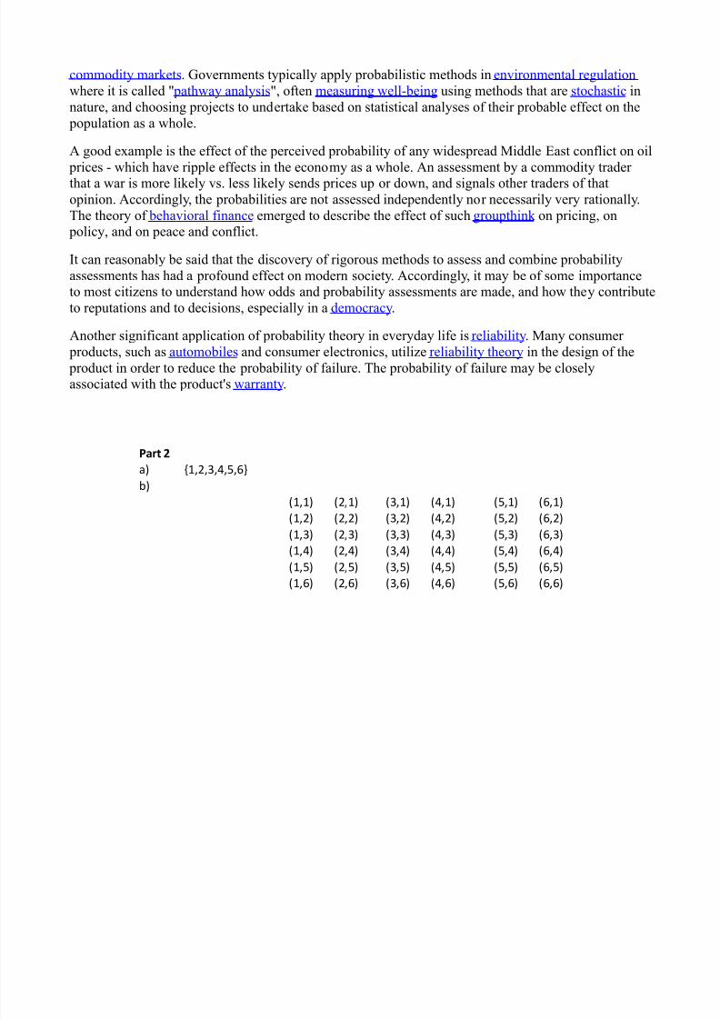
Part 2

a) {1,2,3,4,5,6}

b)

(1,1) (2,1) (3,1) (4,1) (5,1) (6,1)

(1,2) (2,2) (3,2) (4,2) (5,2) (6,2)

(1,3) (2,3) (3,3) (4,3) (5,3) (6,3)(1,4) (2,4) (3,4) (4,4) (5,4) (6,4)

(1,5) (2,5) (3,5) (4,5) (5,5) (6,5)

(1,6) (2,6) (3,6) (4,6) (5,6) (6,6)

8/9/2019 Copy of Additional Mathematics Project 2010

http://slidepdf.com/reader/full/copy-of-additional-mathematics-project-2010 8/14

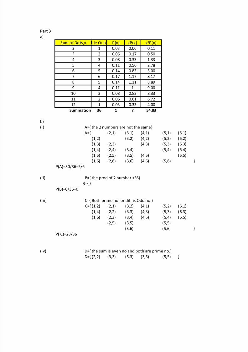
Part 3

a)

Sum of Dots,x ble Outc P(x)

2 1 0.03 0.06 0.11

3 2 0.06 0.17 0.50

4 3 0.08 0.33 1.335 4 0.11 0.56 2.78

6 5 0.14 0.83 5.00

7 6 0.17 1.17 8.17

8 5 0.14 1.11 8.89

9 4 0.11 1 9.00

10 3 0.08 0.83 8.33

11 2 0.06 0.61 6.72

12 1 0.03 0.33 4.00

Summation 36 1 7 54.83

b)(i) A={ the 2 numbers are not the same}

A={ (2,1) (3,1) (4,1) (5,1) (6,1)

(1,2) (3,2) (4,2) (5,2) (6,2)

(1,3) (2,3) (4,3) (5,3) (6,3)

(1,4) (2,4) (3,4) (5,4) (6,4)

(1,5) (2,5) (3,5) (4,5) (6,5)

(1,6) (2,6) (3,6) (4,6) (5,6) }

P(A)=30/36=5/6

(ii) B={ the prod of 2 number >36}

B={ }P(B)=0/36=0

(iii) C={

C={ (1,2) (2,1) (3,2) (4,1) (5,2) (6,1)

(1,4) (2,2) (3,3) (4,3) (5,3) (6,3)

(1,6) (2,3) (3,4) (4,5) (5,4) (6,5)

(2,5) (3,5) (5,5)

(3,6) (5,6) }

P( C)=23/36

(iv) D={ the sum is even no and both are prime no.)

D={ (2,2) (3,3) (5,3) (3,5) (5,5) }

xP(x) x2P(x)

Both prime no. or diff is Odd no.)

8/9/2019 Copy of Additional Mathematics Project 2010

http://slidepdf.com/reader/full/copy-of-additional-mathematics-project-2010 9/14

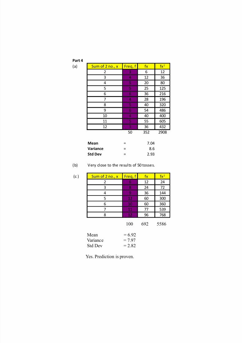
100 692 5586

 

Mean = 6.92

Variance = 7.97Std Dev = 2.82

 Yes. Prediction is proven.

Part 4

(a) Sum of 2 no., x Freq, f fx

2 3 6 12

3 4 12 36

4 5 20 80

5 5 25 125

6 6 36 216

7 4 28 196

8 5 40 320

9 6 54 486

10 4 40 400

11 5 55 605

12 3 36 432

50 352 2908

Mean = 7.04

Variance = 8.6

Std Dev = 2.93

(b) Very close to the results of 50 tosses.

(c ) Sum of 2 no., x Freq, f fx

2 6 12 24

3 8 24 72

4 9 36 144

5 12 60 300

6 10 60 360

7 11 77 539

8 12 96 768

fx2

fx2

8/9/2019 Copy of Additional Mathematics Project 2010

http://slidepdf.com/reader/full/copy-of-additional-mathematics-project-2010 10/14

Part 5

(a) Mean = Σ xP(x) = 7

Variance = Σ x2P(x) - (mean)2

= 5.82

Std Dev = 2.41

(b) Theoretical and practical values are very close. The minor discrepancy is due to bias of the dice

used.The std deviation may vary slightly due to number of sample size used in the experiment.

If the sample size ( number of tossess) is huge, standard dediation tends

to be lower or closer to the theoretical value. Basically as sample size is greater than 25,

the standard deviation discrepeancy getting negligible.

(c ) By both theoretical and experimental practise, the mean will not fluctuate too much as n c

hanges.

By probability,

99.73% coonfidence level, the mean will fall within +/- 3Sigma;-0.24 < mean < 14.24 ( out of range of dice)

95.45% coonfidence level, the mean will fall within +/- 2Sigma;

2.18 < mean < 11.8268.27% coonfidence level, the mean will fall within +/- 2Sigma;

4.59 < mean < 9.41

8/9/2019 Copy of Additional Mathematics Project 2010

http://slidepdf.com/reader/full/copy-of-additional-mathematics-project-2010 11/14

  FUTHER EXPLORATION

In probability theory, the law of large numbers (LLN) is atheorem that describes the resultof performing the same experiment a large number of times. According to the law,

theaverage of the results obtained from a large number of trials should be close tothe expected value, and will tend to become closer as more trials are performed.

For example, a single roll of a six-sided die produces one of the numbers 1, 2, 3, 4, 5, 6, each

with equal probability. Therefore, the expected value of a single die roll is

According to the law of large numbers, if a large number of dice are rolled, the average of 

their values (sometimes called the sample mean) is likely to be close to 3.5, with the

accuracy increasing as more dice are rolled.

Similarly, when a fair coin is flipped once, the expected value of the number of heads is

equal to one half. Therefore, according to the law of large numbers, the proportion of 

heads in a large number of coin flips should be roughly one half. In particular, the

proportion of heads after n flips will almost surely converge to one half as n approaches

infinity.

Though the proportion of heads (and tails) approaches half, almost surely the absolute

(nominal) difference in the number of heads and tails will become large as the number of 

flips becomes large. That is, the probability that the absolute difference is a small number 

approaches zero as number of flips becomes large. Also, almost surely the ratio of the

absolute difference to number of flips will approach zero. Intuitively, expected absolute

difference grows, but at a slower rate than the number of flips, as the number of flips

grows.

The LLN is important because it "guarantees" stable long-term results for random events.

For example, while a casino may lose money in a single spin of the roulette wheel, its

earnings will tend towards a predictable percentage over a large number of spins. Any

8/9/2019 Copy of Additional Mathematics Project 2010

http://slidepdf.com/reader/full/copy-of-additional-mathematics-project-2010 12/14

winning streak by a player will eventually be overcome by the parameters of the game. It

is important to remember that the LLN only applies (as the name indicates) when a large

number of observations are considered. There is no principle that a small number of 

observations will converge to the expected value or that a streak of one value will

immediately be "balanced" by the others.

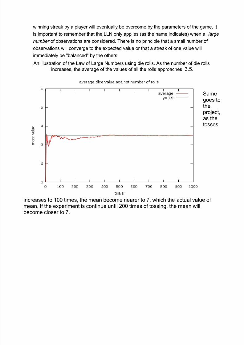
An illustration of the Law of Large Numbers using die rolls. As the number of die rolls

increases, the average of the values of all the rolls approaches 3.5.

 

Samegoes totheproject,

as thetosses

increases to 100 times, the mean become nearer to 7, which the actual value of mean. If the experiment is continue until 200 times of tossing, the mean willbecome closer to 7.

8/9/2019 Copy of Additional Mathematics Project 2010

http://slidepdf.com/reader/full/copy-of-additional-mathematics-project-2010 13/14

REFLECTION

8/9/2019 Copy of Additional Mathematics Project 2010

http://slidepdf.com/reader/full/copy-of-additional-mathematics-project-2010 14/14