Coordination and Policy Moderation at Midtermsekhon.berkeley.edu/papers/midterm/midterm.pdf · Coordination and Policy Moderation at Midterm WALTER R. MEBANE, JR. Cornell University

American Political Science Review Vol. 96, No. 1 March 2002

Coordination and Policy Moderation at MidtermWALTER R. MEBANE, JR. Cornell UniversityJASJEET S. SEKHON Harvard University

Eligible voters have been coordinating their turnout and vote decisions for the House of Represen-tatives in midterm elections. Coordination is a noncooperative rational expectations equilibrium.Stochastic choice models estimated using individual-level data from U.S. National Election Studies

surveys of the years 1978–1998 support the coordinating model and reject a nonstrategic model. Thecoordinating model shows that many voters have incentives to change their votes between the presidentialyear and midterm after learning the outcome of the presidential election. But this mechanism alone doesnot explain the size of midterm cycles. The largest source of loss of support for the president’s party atmidterm is a regular pattern in which the median differences between the voters’ ideal points and theparties’ policy positions have become less favorable for the president’s party than they were at the time ofthe presidential election (nonvoters show the same pattern). The interelection changes are not consistentwith the theory of surge and decline.

Do Americans coordinate their electoral choicesin midterm congressional elections? We use co-ordination to describe a situation in which two

conditions hold for everyone who is eligible to vote (i.e.,every elector). Each elector combines information thateach elector has privately with information that every-one has in common to make the best possible predictionof the election outcome, and each elector makes thechoice—consistent with the elector’s prediction—thatis most likely to produce the best possible result for theelector. Each elector’s prediction takes into accountwhat all electors’ best strategies would be given the in-formation they have in common, a condition describedby saying that each elector has rational expectations.The choice each elector makes is part of the elector’sprivate information. When every elector makes choicesaccording to a strategy that is consistent with the elec-tor’s rational expectations, and no elector can producea personally better outcome by using a different strat-egy, then there is a noncooperative equilibrium. Coor-dination is defined as the existence of a noncooperativeequilibrium that is based on everyone having rationalexpectations.

Beyond implications for the regularity with which thepresident’s party loses vote share in midterm elections,which we discuss below, the existence of coordinationis important because coordination implies that elec-tors take one another into account in a constitutionally

Walter R. Mebane, Jr., is Associate Professor, Department ofGovernment, Cornell University, Ithaca, NY 14853-4601 ([email protected]). Jasjeet S. Sekhon is Assistant Professor, GovernmentDepartment, Harvard University, 34 Kirkland Street, Cambridge,MA 02138 ([email protected]).

Earlier versions of this paper were presented at the 2000 AnnualMeeting of the Midwest Political Science Association, April 27–30,Palmer House, Chicago, at the 1999 Annual Meeting of the AmericanPolitical Science Association, September 2–5, Atlanta, and at semi-nars at Harvard University. Data were made available in part by theCornell Institute for Social and Economic Research and the Inter-university Consortium for Political and Social Research. We thankJonathan Wand for helpful comments, Jonathan Cowden for lettingtron help macht and lapo with the computing, and Gary Jacobsonfor giving us his candidate quality data for the 1978–1998 midtermelections. All errors are solely the responsibility of the authors.

significant way. In American elections, coordination isbased on the separation of powers between the pres-ident and the Congress. Coordination occurs whenelectors anticipate how election outcomes will affectbargaining about policy within the legislature and be-tween the legislature and the executive. By institutingthe constitutional separation of powers, Madison be-lieved that elected officials’ pursuit of their selfish inter-ests and ambitions would lead them to act with regard toone another in ways that would prevent governmentaltyranny (Carey 1978, 159–60). Even electors who didnot coordinate might hope, with Madison, that the sep-aration of powers would affect officials in that way. Butif coordination exists, electors are not mere observersof consequences the constitutional provisions may pro-duce but instead are agents who are led to counteractone another by the constitutional incentives. Coordi-nating electors are as wary of one another as they areof officials.

Coordination produces policy moderation. An elec-tor is acting to moderate policy when the electorchooses what to do based on the idea that, via theinstitutional structure, the policy outcome will be in-termediate between the parties’ positions. With coor-dination it is not that electors individually prefer tohave government produce moderate policy. Indeed, noelector prefers moderation or divided government perse. Rather, the separation of powers and the institutionsthat create public information together channel eachelector’s selfish efforts in such a way that collectivelythere is a moderated result.

In the strategic theory of policy moderation intro-duced by Alesina and Rosenthal (1989, 1995, 1996),which motivates our analysis, each voter’s rationalexpectation about the midterm outcome is part ofa noncooperative equilibrium that encompasses thepresidential and midterm elections. Based on empiricaltests of a rational expectations noncooperative equi-librium model of voters’ choices among candidatesfor president and for the House of Representatives,Mebane (2000) argues that there is coordination amongvoters in presidential elections. We use an extensionof Mebane’s (2000) fixed-point methods to develop an

141

Coordination and Policy Moderation at Midterm March 2002

equilibrium model for turnout and vote choice deci-sions by midterm electors. We test the model usingNational Election Studies (NES) survey data from thesix midterm elections of years 1978 through 1998. Wealso compare the coordinating model explicitly to aninstitutional balancing model that asserts that electorsdo not act strategically. Finally, we examine how wellthe coordinating model explains midterm loss (Erikson1988), taking into account the alternative theory ofsurge and decline (Born 1990; Angus Campbell 1966;James E. Campbell 1987, 1991).

Our analysis is a counterexample to Green andShapiro’s (1994, 195) claim that “rational choice the-ory fares best in environments that are evidence poor.”Indeed, we sharply test the strategic theory using ex-actly the kind of survey data with which Green andShapiro (1994, 195) assert that “rational choice theo-ries have been refuted or domesticated.” Our analysis isnot subject to the pathologies that Green and Shapiroshow have generally afflicted rational choice theory.The statistical model we use to confront the surveydata is isomorphic to the formal equilibrium theory. Wetest the parameters of the estimated model for internalcoherence and the model as a whole against a relevantalternative, namely the nonstrategic model.

It may be surprising to many, including some formaltheorists, that voters are able to behave in the strategicfashion our model posits. No one disputes the long-established fact that most voters are politically ignorant(e.g., Adams [1805] 1973; Bryce [1888] 1995; Converse1964; Delli Carpini and Keeter 1996). What widespreadvoter ignorance implies is controversial, however. Eventhough individuals are poorly informed, political andelectoral institutions may allow voters to make deci-sions that are much the same as they would make ifthey had better information. For instance, McKelveyand Ordeshook (1985a,b) suggest that polls and interestgroup endorsements may perform such cuing functions.Mebane (2000) regards such institutions as implicitlyproviding foundations for coordination, and so do we.It is clear, however, that neither such cues nor the aggre-gate cancellation of individual voter errors is sufficientto produce election results that fully match what wouldhappen if all electors were better informed (Bartels1996).

That electors interact strategically does not implythat they live up to the democratic ideal of being activeparticipants in a rational–critical discourse on public is-sues (Habermas [1964] 1989, [1981] 1984, [1981] 1987).The noncooperative framework takes preferences asgiven, and when assessing the efficacy and desirabilityof possible actions, strategic electors know that they areinteracting with others who are similarly rational. Indiscourse, individuals may modify their preferences inresponse to arguments, and if engaged in communica-tive action, they are “coordinated not through egocen-tric calculations of success but through acts of reachingunderstanding” (Habermas [1981] 1984, 285–6). Com-municative reasoning is about individuals together re-flecting on background assumptions about the worldand bringing shared basic norms to the fore to bequestioned and negotiated. Even if strategic electors

might be thought to be Madisonian because the consti-tutional separation of powers causes them collectivelyto moderate policy, instrumental rationality has indi-viduals taking background assumptions and norms forgranted, as common knowledge, and focusing on pur-suit of gains.

OVERVIEW

We assume that each elector has the same basic insti-tutional understanding that is attributed to voters inthe theories of Alesina and Rosenthal (1995, 1996) andMebane (2000). Each elector knows that postelectionpolicy outcomes are compromises between the posi-tions taken by the president and the Congress, andeach elector believes that the two political parties pushfor distinct policy alternatives. In our theory differentelectors have different beliefs about what the parties’policy positions are, and not all electors care about thepolicy outcomes. An elector may vote for one of theparties or not vote.

The equilibrium concept in our model is similarto Mebane’s (2000): each elector is able to make anequilibrium strategic choice that is based on accurateexpectations regarding the aggregate results of otherelectors’ intended choices.1 Different electors have be-liefs about the upcoming election results that are sim-ilar because of common knowledge all electors havebut differ because of private information each elec-tor has. Our equilibrium includes the level of turnoutalong with the two-party split of votes for House can-didates. The fixed-point values determined in the em-pirical analysis estimate the aggregate values that arecommon knowledge in equilibrium in the theoreticalmodel.

We compare the coordinating model to an empiri-cal model derived from the nonstrategic theory thatFiorina (1988, 1992, 73–81) introduced to describe in-stitutional balancing by voters in elections during pres-idential years. Mebane (2000) finds the nonstrategicmodel to be significantly inferior to his coordinatingmodel in NES data from presidential election years1976–1996. Our findings for the midterms data aresimilar.

One of the most important implications of Alesinaand Rosenthal’s theory is an explanation of midtermloss. According to their theory, some who voted for acongressional candidate of the president’s party whenthe presidential outcome was uncertain would havevoted for the other party had they known which pres-idential candidate would win. At midterm such voterschange their votes, so the president’s party loses con-gressional vote share. Alesina and Rosenthal (1989,1995; Alesina et al. 1993) show patterns in aggre-gate data that in several respects match the kind ofmidterm cycle their theory implies, but, as they observe,the midterm cycle occurs too frequently to be fullyconsistent with their theoretical model (Alesina and

1 Mebane’s (2000) analysis of presidential and House candidatechoices in presidential election years considers only voters.

142

American Political Science Review Vol. 96, No. 1

Rosenthal 1995, 207).2 We use the data and parameterestimates from our model and from Mebane (2000) toconfirm that the disappearing uncertainty of Alesinaand Rosenthal’s theory accounts for only a small partof the midterm cycles that occurred between 1976 and1998. The predominant part of the explanation for thefrequency and magnitude of the midterm cycles is a reg-ular pattern of interelection changes in the relationshipbetween voters’ policy ideal points and the policy posi-tions they attribute to the parties. Usually the changeswork against candidates of the president’s party, but in1998 the changes helped Democrats achieve a midtermgain.

An alternative explanation for midterm loss is thetheory of surge and decline. The details of the the-ory vary somewhat in different accounts (Born 1990;Angus Campbell 1966; James E. Campbell 1987, 1991;Kernell 1977), but there are two central ideas. First,there are people who turn out in the presidential elec-tion and vote for House candidates of the party thatwins the presidency but who do not vote at midterm.Second, presidential coattails cause many voters tochoose House candidates of the president’s party, but atmidterm, absent presidential coattails, the president’sparty suffers a predictable and regular midterm lossproportional to the party’s prior presidential vote mar-gin (Campbell 1991).

One formulation of the surge and decline argumenthighlights the claim that Independents are more likelyto vote in the presidential election than at midterm,so that the midterm electorate consists of a higherproportion of party identifiers whose vote choices arerelatively unmoved by short-run concerns (Campbell1966). Using NES data, Born (1990) finds little supportfor that or related claims about turnout variations. Wefind that policy evaluations change systematically be-tween the presidential election and midterm in waysthat do not match the theory. Consistent with surgeand decline, Born (1990) finds that short-run concernsmatter more during the presidential election than atmidterm. We explain that this asymmetry arises be-cause retrospective economic evaluations significantlyaffect House votes in presidential years, but theseevaluations do not significantly affect House votes atmidterm.

A negative voting variant of the surge and declinetheory argues that voters weigh negative aspects of apresident’s performance more heavily than positive as-pects (Bloom and Price 1975; Kernell 1977). Severalstudies find mixed support for various interpretationsof the negative voting idea (Abramowitz 1985; Cover1986), but Fiorina and Shepsle (1989) show that evi-dence of negative voting reflects nothing more than atechnical artifact. Born (1990) rejects the idea based onNES data from several elections. Because of the lack

2 Scheve and Tomz (1999) use NES panel data to study the rela-tionship between surprise about the presidential election outcomeand midterm loss. As a test of Alesina and Rosenthal’s theory theiranalysis is limited because they do not distinguish policy preferencesfrom party identification and do not impose equilibrium conditionson voters’ beliefs or strategies.

of evidence for asymmetric negative voting, we do notdirectly engage this variant of surge and decline.

The negative voting variant claims to explain aninteresting regularity that surge and decline other-wise does not. A party consistently receives a highervote proportion in midterm House elections whenthe other party controls the White House than whenthey themselves control it. Surge and decline comparesmidterm election returns to the previous presidentialelection but usually ignores the distribution of returnsacross midterms. Our moderation theory explains thatdistribution and, unlike negative voting, has strongindividual-level support.

A MODEL OF COORDINATION IN TURNOUTAND VOTE CHOICES AT MIDTERM

In a manner similar to that of Mebane (2000), the modelof coordination we develop is based on a fixed-pointtheorem that defines the common knowledge beliefthat all electors have about the upcoming election re-sults. The values of two aggregate statistics summarizethe election results: (i) the proportion of the two-partyvote to be cast nationally for Republican candidatesfor the House and (ii) the proportion of electors whowill vote. Our theory differs from Mebane’s by in-cluding electors whose election-time preferences andhence strategies do not depend on expected postelec-tion policies. Each elector who does care about thepolicies responds to the belief each has about the ag-gregate values, because the values affect the loss eachexpects.

The election is a game among everyone who is eli-gible to vote, that is, among all the electors, assumedto be a large number. Electors act noncooperativelyand simultaneously, each choosing whether to vote fora Democratic or a Republican candidate for a Houseseat or not to vote. In some House districts a candidatemay be unopposed. Every elector’s expectations aboutthe election outcome depend on the strategies otherelectors are expected to use. Equilibrium occurs whenevery elector uses all available information to form suchexpectations and, given everything each elector knows,no elector expects to gain by using a different strategy.In the following discussion we sketch the main featuresof the model. Further details, including the extensionto include unopposed candidates in some districts, aregiven in the Appendix.

Elector i expects that after the election Democratswill try to implement policy position θDi and Republi-cans position θRi . Given expectations that a proportionVi of the N electors will vote and a proportion Hi ofthe vote will go to Republicans, i expects postelectionpolicy to be

θi =

αθDi + (1 − α)[HiθRi + (1 − Hi )θDi ],if Democrat is president,

αθRi + (1 − α)[HiθRi + (1 − Hi )θDi ],if Republican is president,

143


where α, 0 ≤ α ≤ 1, represents the president’s strengthin comparison to the House, and HiθRi + (1 − Hi )θDiis the position i expects the House to take. If electori ’s preferences depend on policy, then i ’s expected lossfrom θi , denoted λi , depends on i ’s ideal point θi , ac-cording to λi = |θi − θ i |q, where 0 < q < +∞, and weset an indicator variable γi = 1.3 If i does not care aboutpolicy, then λi = 0 and we set γi = 0.

Every elector’s choice—whether to vote for the Re-publican, to vote for the Democrat, or not to vote—affects Hi and hence affects θi . We write Hi = Hi,R ifi votes Republican and Hi = Hi,D if i votes Democrat,with Hi,R > Hi,D. The effect an increase in Hi has onλi is

wCi =

q(θDi − θRi )(1 − α)|θi − θi |q−1 sgn(θi − θi ),if γi = 1,

0, if γi = 0,

where sgn(x) = −1 if x < 0, sgn(x) = 0 if x = 0, andsgn(x) = 1 if x > 0. Each choice also involves additionalgains and losses, such that the total loss for i is

λi =

λi,D + zi,D + εi,D, if i votes for the Democrat,λi,R + zi,R + εi,R, if i votes for the Republican,

λi,A + zi,A + εi,A, if i does not vote.

To minimize λi , i chooses the value from the set K ={D, R, A} that minimizes xi,h + εi,h, h ∈ K, where D de-notes voting for the Democrat, Rvoting for the Repub-lican, and A not voting, and, using Vi,A to denote thevalue of Vi if i does not vote,

xi,D = −(NVi,A)−1 Hi,DwCi + zi,D, (1a)

xi,R = (NVi,A)−1(1 − Hi,R)wCi + zi,R, (1b)

xi,A = zi,A. (1c)

Variable Yi denotes i ’s choice from K. Because Yi de-pends on Vi and Hi , the best choice for each electorwho has γi = 1 depends on what i expects others to do.Yi is an equilibrium only if it minimizes λi when each iassumes that everyone else is using the same rule andonly if it is supported by every i believing “mutuallyconsistent” (Mebane 2000, 41) values for Hi and Vi .The definition of Yi and assumptions we make aboutthe probability distribution of wCi , zi,h, and εi,h implychoice probabilities µi,D, µi,R, and µi,A.

We use Mebane’s (2000) method to characterizeeach mutually consistent pair (Hi , Vi ) as a deviation

3 In Mebane’s (2000) coordinating model, the weight each voterplaces on the expected policy-related loss from each party dependson the voter’s retrospective evaluation of the national economy (seeMebane’s Eqs. 3 and 16). In alternative specifications, not reportedhere, estimation of the stochastic choice model [see Eqs. (2a)–(2c)and (A7) and (A8) in the Appendix] showed no evidence of suchdependence in the expected policy-related losses of midterm electors.Hence we have simplified the definition of the midterm theoreticalmodel.

from common knowledge expections (H, V) that allelectors have when each elector i knows only thedistribution of wCi , zi,h, and εi,h. In that case, theproportions of electors expected to vote Republicanand Democratic are, respectively, R and D such thatV = R+ D, H = R/V and, in (1a) and (1b), Vi,A= Vand Hi,D = Hi,R = H, and i ’s choice probabilities areµki ,h = µk,h (same for all i in a set indexed by k). Thedifference between (Hi , Vi ) and (H, V) reflects i ’s pri-vate information, which is the actual values of wCi ,zi,h, and εi,h. Let yi,h indicate the value of Yi when iknows wCi , zi,h, and εi,h, h ∈ K, but for other electors hasonly the common knowledge: yi,h = 1 if Yi = h, yi,h = 0if Yi �= h, h ∈ K. Define Riyi,R = R + (yi,R − µki ,R)/N,Diyi,D = D + (yi,D − µki ,D)/N, Viyi,Ryi,D = Riyi,R + Diyi,D,and Hiyi,Ryi,D = Riyi,R/Viyi,Ryi,D. A set of equilibriumchoices Yi and expectations (Hi , Vi ), i = 1, . . . , N, isgiven by the following theorem.

THEOREM 1. There is a coordinating elector equi-librium if, with all electors using the same fixedpoint (H, V) computed from common knowledge,each elector i has (Hi , Vi ) = (Hiyi,Ryi,D, Viyi,Ryi,D) andYi = h, h ∈ K, for whichever of the three possiblepairs of values (Hiyi,Ryi,D, Viyi,Ryi,D) corresponds tothe smallest value of λi : either Hi = Hi01, Vi = Vi01,and Yi = D; Hi = Hi10, Vi = Vi10, and Yi = R; orHi = Hi00, Vi = Vi00, and Yi = A.

A COORDINATING MODEL FORSURVEY DATA

With survey data we observe choices Yi ∈ K reportedby each elector i in a sample S of size n, i = 1, . . . , n, anda set of variables Zi that affect electoral choices. GivenZi and a set of parameter values, we adapt Mebane’s(2000) method to compute values ( ˆH, ˆV). In (1a)–(1c)we set Hi = ˆH and Vi = ˆV and substitute bC

ˆV−1 for(NV)−1, where bC > 0 is a constant parameter:

xi,D = −bCˆV−1 ˆHwCi + zi,D, (2a)

xi,R = bCˆV−1(1 − ˆH)wCi + zi,R, (2b)

xi,A = zi,A. (2c)

Further details, including the definition of the log-likelihood, are given in the Appendix.

We test whether the parameters satisfy conditionsnecessary for coordination to exist. If α = 1, thenwCi = 0 so that electors’ strategies depend on neitherˆH nor ˆV and there is no coordination. We use confi-

dence intervals and likelihood-ratio (LR) tests to checkwhether α = 1 can be rejected for each year of our data.We use Davies’s (1987, 36, Eq. 3.4) method to adjust theLR test significance probabilities for a nonregularitythat arises because the model does not depend on ρwhen α = 1. Also necessary for the model to describecoordination are that q > 0 and that bC > 0: q = 0 imp-lies that wCi = 0, and bC = 0 implies that wCi , ˆH and ˆVdo not affect i ’s choice.

144


A NONSTRATEGIC MODERATING MODEL

To test further whether electors coordinate, we definean empirical model that applies to midterm electionsthe core idea in Fiorina’s (1988, 1992, 73–81) non-strategic theory of institutional balancing by voters inpresidential-year elections. The theory considers a sit-uation in which each voter has a choice between twocandidates for president and two candidates for thelegislature, one from each of two parties. Each voterchooses the mix of party control of the presidencyand the legislature, either unified or divided govern-ment, that would produce a policy outcome nearest theelector’s ideal point. The voter ignores the expectedelection outcome. The theory is nonstrategic becauseno voter’s choice depends on the likely choice of anyother voter.

We apply the nonstrategic theory by assuming thatat midterm each elector i treats the party of the presi-dent as fixed in forming a preference between unifiedor divided government but ignores the expected elec-tion outcome. The postelection policies that i expectsif there is a Democratic majority in the House are4

θDi =

θDi , if Democrat is president

αθRi + (1 − α)θDi ,

if Republican is president

(3)

and the postelection policies that i expects if there is aRepublican majority are

θRi =

αθDi + (1 − α)θRi ,

if Democrat is president

θRi , if Republican is president

(4)

with 0 ≤ α ≤ 1. The nonstrategic theory says that, otherthings equal, i votes for the Democrat instead of the Re-publican if i ’s ideal point is closer to the policy expectedwith a Democratic majority than to the policy expectedwith a Republican majority, i.e., if |θi − θDi |< |θi − θRi |.If |θi − θDi | > |θi − θRi |, then i votes for the Republicaninstead of the Democrat.

In the nonstrategic model there is policy moderationonly if 0 < α < 1. If α = 1, then the president’s party’sposition is the expected policy, hence θDi = θRi , and pol-icy comparisons do not affect midterm vote choices. Ifα = 0, then θDi = θDi and θRi = θRi regardless of who ispresident. There is no moderation but rather a simplechoice between the parties’ alternative policies.

To include the possibility of not voting, we use thesame log-likelihood function as with the coordinatingmodel, except based on modified definitions of xi,h,h ∈ K. Defining

wNSi ={|θi − θRi |q − |θi − θDi |q, if γi = 1

0, if γi = 0

with 0 < q < +∞, we define

4 θDi and θRi are as defined in the Appendix, Eqs. (A1) and (A2).

xi,D = −bNSwNSi + zi,D (5a)

xi,R = bNSwNSi + zi,R (5b)

xi,A = zi,A (5c)

with bNS ≥ 0. If bNS > 0, then ∂µi,D/∂wNSi > 0 and∂µi,R/∂wNSi < 0.

The coordinating and nonstrategic models differ onlyin that the former uses ˆV−1 ˆHwCi and ˆV−1(1 − ˆH)wCito define xi,D and xi,R, while the latter uses wNSi . We useVuong’s (1989, 320) test to compare them, first testingseparately whether bC > 0 and bNS > 0. The models mayfit the data about equally well because wCi and wNSihave the same sign if θi = (θDi + θRi )/2.

DEFINITIONS OF EMPIRICAL CHOICEATTRIBUTES

To estimate the models we pool NES Survey datafrom the years 1978, 1982, 1986, 1990, 1994 and 1998(Miller and National Election Studies 1979, 1983, 1987;Miller et al. 1992; Rosenstone et al. 1995; Sapiro,Rosenstone, and National Election Studies 1999).Some parameters vary by year.

We use NES 7-point scales and the method describedby Mebane (2000, 55) to determine the values of θi , ϑDi ,ϑRi , and ϑPDi or ϑPRi for each i .5 If an elector i doesnot provide values for the policy position variables (θi ,ϑDi , ϑRi , and ϑPDi or ϑPRi ), we assume that i does notexperience policy-related losses, so that such losses donot affect the choices i makes. We set γi = 0 if there isnot at least one complete set of policy position variablevalues for i and γi = 1 if at least one complete set exists.6We include γi in zi,A. To allow for the possibility ofideologically based mobilization, we also include eachelector’s ideal point in zi,A, using the form γiθi to switchthe effect off when i lacks a complete set of policy po-sition values.

Evidence that retrospective economic evaluationsmatter in presidential elections is strong, but systematicdirect effects seem not to exist for candidate choices inHouse elections at midterm (Alesina and Rosenthal1989; Born 1991; Erikson 1990; Jacobson 1989). Effectson turnout decisions also have been found to be weak

5 The NES variables for each set of scales for each year are givenhere. “Reversed” indicates an item for which we reversed the original1–7 ordering. In years 1982–1998 respondents who initially declinedto place themselves on the Liberal/Conservative scale, or who ini-tially described themselves as “moderate” on the scale, were askeda follow-up question; we used those responses to categorize themas either “slightly liberal,” “moderate,” or “slightly conservative.”1978: 357–360; 365–368; 373–376; 381–384; 389–392; 399–402. 1982:393, 394, 404–406; 407–410; 415–418; 425–428; 435–438; reversed 443–446. 1986: 385–387, 393, 394; 405, 406, 412, 413; 428, 429, 435, 436;reversed 448, 449, 455, 456. 1990: 406–408, 413, 414; 439, 440, 443,444; 447–450; reversed 452, 453, 456, 457. 1994: 839–841, 847, 848;930, 931, 934, 935; 936–939; reversed 940, 941, 944, 945; 950, 951, 954,955. 1998 (omitting the prefix “980”): 399, 401, 403, 411, 412; 448, 449,453, 454; 457, 458, 460, 461; reversed 463, 464, 468, 469.6 There is a “complete set” if i placed all four of the referents forany single scale topic, e.g., placing self, the parties, and the presidenton the scale for Rights of the Accused (variables 365–368) in 1978.Among the cases used to compute the estimates reported in Table 1,the percentage with γi = 0 is, by year, 14.2, 10.9, 10.9, 12.2, 4.8, and5.0.

145


(Arcelus and Meltzer 1975; Fiorina 1978). To measureretrospective evaluations we use responses to a ques-tion asking whether the national economy has gottenworse or better over the past year.7 In zi,D, zi,R, and zi,Awe include the variable, ECi , multiplied by PPi = 1 ifthe president is Republican; PPi = −1 if Democrat.

Party identification has long been known to af-fect vote choices (e.g., Campbell and Miller 1957)and to be associated both with varying rates of voterturnout (Campbell 1966; Converse 1966; Miller 1979)and with policy preferences and perceptions (Bradyand Sniderman 1985). We measure party identificationwith six dummy variables that correspond to the levelsof the NES 7-point scale, using “Strong Democrat” asthe reference category: PIDDi , PIDIDi , PIDIi , PIDIRi ,PIDRi , and PIDSRi .8 We include the variables in zi,D,zi,R, and zi,A.

To take incumbent-related effects into account, weuse a pair of dummy variables that indicate whethera Democratic or Republican incumbent is runningfor reelection in elector i ’s congressional district.DEMi = 1 if a Democratic incumbent is running, oth-erwise DEMi = 0, and likewise for REPi and a Repub-lican incumbent.9 In the choice between candidates weexpect to see an incumbency advantage.10 Because thepresence of an incumbent usually means the absenceof a vigorous campaign, the probability of not votingshould be higher when an incumbent is running thanwhen there is an open seat.11

We include in zi,A a measure of subjective politicalefficacy (EFFi ), defined as the average of responsesto two survey items (Abramson and Aldrich 1982;Balch 1974),12 and four demographic variables that arefrequently observed to have strong effects on voterturnout (Born 1990): education, age, marital status,and time at current residence. Three dummy variablesmeasure education: high school diploma, 12+ yearsof school, no higher degree (ED1i ); AA- or BA-leveldegrees or 17+ years of school and no higher degree

7 By year, the NES variables are 338, 328, 373, 423, 909, and 980419.Codes are as given by Mebane (2000, 55).8 By year, the NES variables are 433, 291, 300, 320, 655, and 980339.9 By year, the NES variables are 4, 6, 43, 58, 17, and 980065.10 Eubank and Gow (1983) and Gow and Eubank (1984) documentproincumbent biases in 1978 and 1982 NES data. Estimated incum-bency effects may be exaggerated (cf. Eubank 1985).11 Including dummy variables based on Jacobson’s (1989) candidatequality measure improves the fit to the data but does not change anyof the results of primary interest in the analysis.12 The items are “have say” and “don’t care much.” By year, theNES variables are as follows: 351, 354; 531, 532; 549 (“don’t care”);509, 508; 1038, 1037; and 980525, 980524. In 1978, 1982, and 1986, theresponse codes are −1 for “agree” and 1 for “disagree.” In 1990, 1994,and 1998, five responses range from “agree strongly” to “disagreestrongly,” coded −1, −0.5, 0, 0.5 and 1. In 1986 only the “don’t care”item is available, and only for half the sample. We use a proxy variableto replace missing values for variable 549, constructed by summingthe values of four variables: 62, 64, and 66, each being coded 1 if yesand 0 otherwise; and 59, coded 1 if “very interested” or “somewhatinterested” and 0 otherwise. Respondents with INDEX = 4 are as-signed the value 1; those with INDEX <4 are assigned −1. Supportfor the proxy comes from a logistic regression model for the binaryresponses to variable 549 in the half-sample that was asked thatquestion, with INDEX as the regressor: the MLEs give Pr(variable549 = disagree) >0.5 only if INDEX = 4.

(ED2i ); and advanced degree, including LLB (ED3i ).The reference category for the dummy variables is 11grades or less, no diploma, or equivalency. Age we mea-sure as time in year minus 40 (AGEi ). Marital status is adummy variable (MARi ) coded 1 for “married and liv-ing with spouse (or spouse in service)” and 0 otherwise.Time at current residence (RESi ) is measured in wholeyears for durations of between 3 and 9 years; otherwiseit is coded using the same values used by Born (1990):less than 6 months, 0.25; 6–12 months, or 1 year, 0.75;13–24 months, or 2 years, 1.5; and 10 years or more,10.13

The definitions of the attributes of the choices are

zi,D = c0 − cDEMDEMi + cECPPi ECi + cDPIDDi

+ cI DPIDIDi + cIPIDIi + cI RPIDIRi

+ cRPIDRi + cSRPIDSRi , (6a)

zi,R = −c0 − cREPREPi − cECPPi ECi − cDPIDDi

− cI DPIDIDi − cIPIDIi − cI R PIDIRi

− cR PIDRi − cSR PIDSRi , (6b)

zi,A = d0 + dEF F EFFi + dED1ED1i + dED2 ED2i

+ dED3ED3i + dAGEAGEi + dMARMARi

+ dRESRESi + dγ (1 − γi ) + dθγiθi

+ dREPREPi + dDEMDEMi + dEC PPi ECi

+ dDPIDDi + dI DPIDIDi + dIPIDIi

+ dI RPIDIRi + dRPIDRi + dSRPIDSRi , (6c)

where the parameters c0, cEC, d0, dEC, and dθ areconstant in each year, and the remaining parametersare constant over all years. A variable that increasesthe probability of choosing h ∈ K will have a negativecoefficient.14 The effects measured by the c parametersprimarily contrast the candidate alternatives to oneanother, while the d parameters measure effects thatcontrast the choice not to vote to the choice to vote.For the attributes of the candidates, the parameter signsshould be c0 < 0 and cEC, cDEM, cREP, cD, cI D, cI , cI R, cR,cSR > 0. For the attributes of not voting, the parametersigns should be dγ , dREP, dDEM, dD, dI D, dI , dI R, dR < 0and dEF F , dED1, dED2, dED3, dAGE, dMAR, dRES > 0. Thesigns of d0, dθ , and dEC are indeterminate.

To measure choices yi,h we use individuals’ selfreports.15 The sample size of electors used, pooled overthe six NES surveys, is 9639 (by year, 1978–1998, thesizes are 1814, 1226, 1972, 1833, 1648, and 1146, respec-tively.). Only those who did not vote or who voted foreither a Democrat or a Republican are included. Of

13 By year, the NES variables for education, age, marital status, andresidency are as follows: 513, 504, 505, 628; 542, 535, 536, 760; 602,595, 598, 753; 557, 552, 553, 684; 1209, 1203, 1204, 1426; and 980577,980572, 980573, 980662.14 In the Appendix, Eq. (A4): ∂vi,h/∂zi,h < 0.15 By year, the NES variables are as follows: 470, 473, 474; 501, 505,506; 261, 265, 267; 279, 287, 289; 601, 612, 614; and 980303, 980311,980313.

146


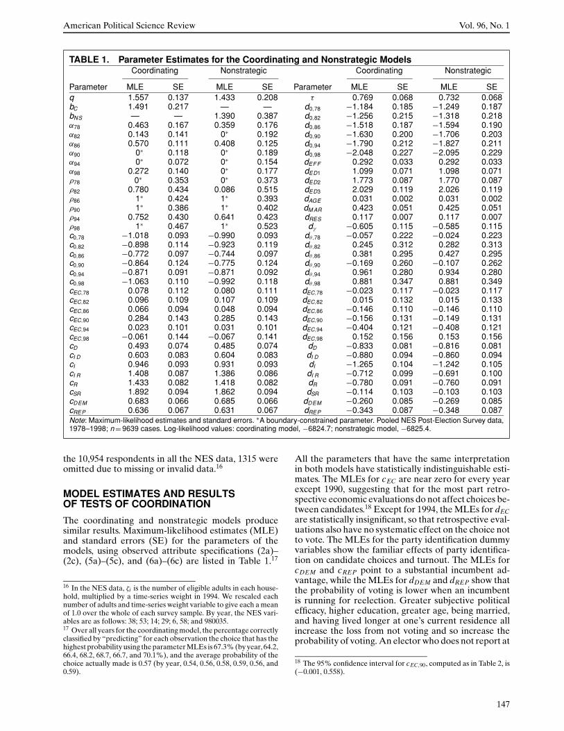
TABLE 1. Parameter Estimates for the Coordinating and Nonstrategic ModelsCoordinating Nonstrategic Coordinating Nonstrategic

Parameter MLE SE MLE SE Parameter MLE SE MLE SEq 1.557 0.137 1.433 0.208 τ 0.769 0.068 0.732 0.068bC 1.491 0.217 — — d0,78 −1.184 0.185 −1.249 0.187bNS — — 1.390 0.387 d0,82 −1.256 0.215 −1.318 0.218α78 0.463 0.167 0.359 0.176 d0,86 −1.518 0.187 −1.594 0.190α82 0.143 0.141 0∗ 0.192 d0,90 −1.630 0.200 −1.706 0.203α86 0.570 0.111 0.408 0.125 d0,94 −1.790 0.212 −1.827 0.211α90 0∗ 0.118 0∗ 0.189 d0,98 −2.048 0.227 −2.095 0.229α94 0∗ 0.072 0∗ 0.154 dEF F 0.292 0.033 0.292 0.033α98 0.272 0.140 0∗ 0.177 dED1 1.099 0.071 1.098 0.071ρ78 0∗ 0.353 0∗ 0.373 dED2 1.773 0.087 1.770 0.087ρ82 0.780 0.434 0.086 0.515 dED3 2.029 0.119 2.026 0.119ρ86 1∗ 0.424 1∗ 0.393 dAGE 0.031 0.002 0.031 0.002ρ90 1∗ 0.386 1∗ 0.402 dM AR 0.423 0.051 0.425 0.051ρ94 0.752 0.430 0.641 0.423 dRES 0.117 0.007 0.117 0.007ρ98 1∗ 0.467 1∗ 0.523 dγ −0.605 0.115 −0.585 0.115c0,78 −1.018 0.093 −0.990 0.093 dθ,78 −0.057 0.222 −0.024 0.223c0,82 −0.898 0.114 −0.923 0.119 dθ,82 0.245 0.312 0.282 0.313c0,86 −0.772 0.097 −0.744 0.097 dθ,86 0.381 0.295 0.427 0.295c0,90 −0.864 0.124 −0.775 0.124 dθ,90 −0.169 0.260 −0.107 0.262c0,94 −0.871 0.091 −0.871 0.092 dθ,94 0.961 0.280 0.934 0.280c0,98 −1.063 0.110 −0.992 0.118 dθ,98 0.881 0.347 0.881 0.349cEC,78 0.078 0.112 0.080 0.111 dEC,78 −0.023 0.117 −0.023 0.117cEC,82 0.096 0.109 0.107 0.109 dEC,82 0.015 0.132 0.015 0.133cEC,86 0.066 0.094 0.048 0.094 dEC,86 −0.146 0.110 −0.146 0.110cEC,90 0.284 0.143 0.285 0.143 dEC,90 −0.156 0.131 −0.149 0.131cEC,94 0.023 0.101 0.031 0.101 dEC,94 −0.404 0.121 −0.408 0.121cEC,98 −0.061 0.144 −0.067 0.141 dEC,98 0.152 0.156 0.153 0.156cD 0.493 0.074 0.485 0.074 dD −0.833 0.081 −0.816 0.081cI D 0.603 0.083 0.604 0.083 dI D −0.880 0.094 −0.860 0.094cI 0.946 0.093 0.931 0.093 dI −1.265 0.104 −1.242 0.105cI R 1.408 0.087 1.386 0.086 dI R −0.712 0.099 −0.691 0.100cR 1.433 0.082 1.418 0.082 dR −0.780 0.091 −0.760 0.091cSR 1.892 0.094 1.862 0.094 dSR −0.114 0.103 −0.103 0.103cDEM 0.683 0.066 0.685 0.066 dDEM −0.260 0.085 −0.269 0.085cREP 0.636 0.067 0.631 0.067 dREP −0.343 0.087 −0.348 0.087Note: Maximum-likelihood estimates and standard errors. ∗A boundary-constrained parameter. Pooled NES Post-Election Survey data,1978–1998; n = 9639 cases. Log-likelihood values: coordinating model, −6824.7; nonstrategic model, −6825.4.

the 10,954 respondents in all the NES data, 1315 wereomitted due to missing or invalid data.16

MODEL ESTIMATES AND RESULTSOF TESTS OF COORDINATION

The coordinating and nonstrategic models producesimilar results. Maximum-likelihood estimates (MLE)and standard errors (SE) for the parameters of themodels, using observed attribute specifications (2a)–(2c), (5a)–(5c), and (6a)–(6c) are listed in Table 1.17

16 In the NES data, ζi is the number of eligible adults in each house-hold, multiplied by a time-series weight in 1994. We rescaled eachnumber of adults and time-series weight variable to give each a meanof 1.0 over the whole of each survey sample. By year, the NES vari-ables are as follows: 38; 53; 14; 29; 6, 58; and 980035.17 Over all years for the coordinating model, the percentage correctlyclassified by “predicting” for each observation the choice that has thehighest probability using the parameter MLEs is 67.3% (by year, 64.2,66.4, 68.2, 68.7, 66.7, and 70.1%), and the average probability of thechoice actually made is 0.57 (by year, 0.54, 0.56, 0.58, 0.59, 0.56, and0.59).

All the parameters that have the same interpretationin both models have statistically indistinguishable esti-mates. The MLEs for cEC are near zero for every yearexcept 1990, suggesting that for the most part retro-spective economic evaluations do not affect choices be-tween candidates.18 Except for 1994, the MLEs for dECare statistically insignificant, so that retrospective eval-uations also have no systematic effect on the choice notto vote. The MLEs for the party identification dummyvariables show the familiar effects of party identifica-tion on candidate choices and turnout. The MLEs forcDEM and cREP point to a substantial incumbent ad-vantage, while the MLEs for dDEM and dREP show thatthe probability of voting is lower when an incumbentis running for reelection. Greater subjective politicalefficacy, higher education, greater age, being married,and having lived longer at one’s current residence allincrease the loss from not voting and so increase theprobability of voting. An elector who does not report at

18 The 95% confidence interval for cEC,90, computed as in Table 2, is(−0.001, 0.558).

147


TABLE 2. Ninety-Five Percent ConfidenceIntervals for α

Lower UpperParameter Bound Boundα78 0.157 0.787α82 0∗ 0.423α86 0.348 0.775α90 0∗ 0.196α94 0∗ 0.127α98 0.007 0.541Note: Estimates are based on tabulation of an asymptoticmixture distribution of the kind derived by Self and Liang(1987), under the hypothesis that α90 = α94 = ρ78 = 0 andρ86 = ρ90 = ρ98 = 1. ∗A boundary-constrained value.

least one complete set of policy position values (γi = 0)is significantly more likely not to vote than an electorwho does report policy positions. For 1994 and 1998,electors who have higher values of θi are significantlymore likely to vote than electors who have lower valuesof θi : conservative electors were especially mobilized inthose elections.

The coordinating model passes the tests of the condi-tions necessary for coordinating behavior. The LR teststatistics for the constraint α = 1, imposed separatelyfor each year, reject the constraint in every year.19 The95% confidence intervals listed in Table 2 support thesame conclusions.20 Regarding the other conditions,95% confidence intervals computed as in Table 2 showq (1.28, 1.81) and bC (1.10, 1.90) to be positive andbounded well away from zero.

The MLEs for the nonstrategic model do not supportthe theory of nonstrategic institutional balancing. Onlytwo of the six MLEs for α (α78 and α86) are statisticallydistinguishable from zero; α82 = α90 = α94 = α98 = 0.Rather than moderating, the estimates suggest that inmost years electors are making direct choices betweenthe parties’ alternative policies.

While the log-likelihood of the coordinating model(−6824.7) is not much greater than that of the non-strategic model (−6825.4), Vuong’s (1989) overlap-ping models test nonetheless rejects the nonstrategicmodel as an alternative to the coordinating model. TheMLEs and SEs in Table 1 clearly reject both bC = 0 andbNS = 0. Using the distribution of Vuong (1989, Eq. 6.4),the test statistic is n−1/2LRn/ωn = 4.3 (p< .0001).21

19 By year, the LR statistics −2(Lconstrained − L) and associated sig-nificance probabilities are 13.2 (p< 0.001), 35.2 (p< 0.0001), 12.0(p< 0.01), 28.6 (p< 0.0001), 53.3 (p< 0.0001), and 26.7 (p< 0.0001).The significance probability is the upper-tail probability for the χ2

1distribution under the null hypothesis α = 1, using the method ofDavies (1987, Eq. 3.4) to adjust for the nuisance parameter ρ.20 Table 1 shows α90, α94, ρ78, ρ86, ρ90, and ρ98 to have MLEs equalto either 0.0 or 1.0, on boundaries of the parameter space. We boot-strap (20,000 resamples) the score vectors of the MLEs in Table 1 toestimate the quantiles of the asymptotic distribution implied by thehypothesis that α90 = α94 = ρ78 = 0 and ρ86 = ρ90 = ρ98 = 1, which isa mixture of 64 censored multivariate normal distributions (Self andLiang 1987) and, hence, estimate the confidence intervals in Table 2.21 LRn = 16.50197 (Vuong 1989, Eq. 3.1) and ω2

n = 0.0014981 −0.00171202 = 0.0014952 (Vuong 1989, Eq. 4.2). We compute bothLRn and ω2

n with adjustments for sampling weights.

MODERATION, INSTITUTIONALBALANCING, AND THE MIDTERM CYCLE

In the coordinating model, every elector anticipates apostelection policy that is intermediate between theparties’ positions, unless α = 1. The coordinating modelMLEs for α are less than 0.5 in every year except 1986(see Table 1), suggesting that electors expected thepresident to be weaker than the House in determiningpostmidterm policy. The estimates for ˆH show that theposition of the House was expected to be closer to theDemocratic position in 1978, 1982, 1986, and 1990 andcloser to the Republican position in 1994 and 1998.22

The systematic foundation for a midterm cycle in thecoordinating model is that the equilibrium RepublicanHouse vote share each elector expects at the time ofthe presidential election is no longer an equilibriumonce the identity of the president becomes known. Thepostelection disequilibrium decreases the probabilitythat each elector votes for a House candidate of thepresident’s party. The aggregation of such changes isthe cycle-generating mechanism.

Does the coordinating model’s moderating mecha-nism, which is based on λi , generate a midterm cycle?For a baseline measure of the effect policy-related in-centives have on choices in the presidential electionyear preceding each midterm, we use Mebane’s (2000,Table 7) estimates of the proportion of presidential-year voters for whom each combination of presidentialand House choices would minimize expected policy-related losses.23 Consider the proportion of voters ina presidential election who would minimize their ex-pected policy-related losses by voting for a House can-didate of the same party as the new president. Thereis a policy-related foundation for a midterm cycle ifthat proportion is greater than the proportion of votersin the subsequent midterm who would minimize theirpolicy-related losses by voting for a candidate of thesame party as the president. Table 3 shows that such apattern occurs for all six midterm elections, althoughthe decline from 1996 to 1998 is considerably smallerthan for the other years.24

It is doubtful, however, whether most of the changein votes from presidential election to midterm is duepurely to the postelection disequilibrium that the disap-pearance of uncertainty about the identity of the presi-dent brings about. Simulation using presidential-yearNES data and Mebane’s (2000) coordinating votingmodel suggests that immediately after the presidentialelection, due solely to the identity of the new presidenthaving become known, the equilibrium proportion of

22 By year, ˆH and ˆV computed using the parameter MLEs in Table 1and 1978–1998 NES data are as follows: 0.393, 0.477; 0.437, 0.550;0.418, 0.481; 0.373, 0.439; 0.544, 0.558; 0.524, and 0.455.23 From Mebane’s (2000) Table 7 coordinating model results we sumthe percentages with choices RR and DR to get the percentage forwhom choosing a Republican House candidate minimizes the ex-pected policy-related loss, and we sum the percentages with choicesDD and RD to get the percentages for whom choosing a Democratminimizes the loss.24 By midterm year, the decreases shown in Table 3 are 0.167, 0.229,0.206, 0.124, 0.278, and 0.028.

148


TABLE 3. House Vote Choices that MinimizePolicy-Related Losses, by Year

Preceding MidtermPresidential Coordinating

Yeara Modelb

D R D RMidterm President’sYear Party1978 D 0.500 0.500 0.333 0.6671982 R 0.337 0.663 0.566 0.4341986 R 0.593 0.407 0.799 0.2011990 R 0.337 0.663 0.461 0.5391994 D 0.635 0.365 0.357 0.6431998 D 0.544 0.456 0.516 0.484Note: Entries show the proportion of voters in each year forwhom a vote for a House candidate of the indicated party isassociated with a smaller policy-related loss than is a vote for theother party. Midterm entries are computed using the parameterMLEs in Table 1 and 1978–1998 NES data. Each observationis weighted by the sampling weight 1/ζi .a Proportion of voters in the preceding presidential election yearfor whom the indicated House candidate choice minimizes theexpected policy-related loss according to the coordinating votingmodel estimates of Mebane (2000, Table 7).b Of voters with γi = 1 and wCi �= 0, the proportion under D havewCi > 0 and the proportion under R have wCi < 0.

House votes for the new president’s party typicallyfalls by values ranging from about 0.01 to about 0.06.25

The simulated loss is substantially smaller than the cor-responding decrease in policy-related support for thepresident’s party shown in Table 3 for each midtermyear except 1998. Other factors that change betweenthe presidential and the midterm elections are modulat-ing the magnitude of the policy-related midterm losses.Such factors include the fact that the president is usuallyexpected to have less influence on policy after midtermthan after the preceding presidential election.26 Theform of each elector’s evaluation of the policy-relatedlosses also changes: at midterm an elector’s evaluationof λi does not depend on the elector’s retrospectiveevaluation of the economy, as it does in presidentialelection years.27 And between elections parties maychange their policy positions, or voters may changetheir ideal points, and substantively different policiescome into play.

SURGE AND DECLINE

The theory of surge and decline suggests a possible rea-son for the relationship between voters’ most preferred

25 The simulation consists of recomputing the choice probabilities ofMebane’s (2000) empirical coordinating model with P set equal to0 or 1 depending on which party actually won the presidency in eachelection. By presidential year, 1976–1996, the losses for the new pre-sident’s party are 0.011, 0.060, 0.015, 0.035, 0.043, and 0.058.26 The upper bounds of the 95% confidence intervals for α, in Table 2,are smaller than the lower bounds of the 95% confidence intervalsthat Mebane (2000, Table 4) reports for αD or αR for the winningpresidential candidate for all years except 1984. The interval for αR,84,(0.34, 0.79), is virtually the same as the interval for α86 in Table 2,suggesting that voters believed that Reagan’s influence on policyremained about the same throughout his second term.27 Recall footnote 3.

policies and the policy positions they attribute to theparties to change in a systematic way between the pres-idential and the midterm elections. According to thetheory, during the heightened mobilization of presi-dential elections more electors with marginal politicalinvolvement turn out to vote than during midterm elec-tions, and this group disproportionately votes for theparty of the winning presidential candidate (Campbell1966). Campbell’s (1987) revised theory treats midtermas a return to a normal partisan vote, less influencedby short-run concerns than the presidential election.He writes, “Surge of interest and information in pres-idential elections will affect the turnout of peripheralpartisans and the vote choice of independents” (p. 968).Born (1990, 642, note 30) raises serious doubts aboutthose revisions.

Perhaps the surge of marginal electors who, accord-ing to the theory, vote for House candidates of thesame party as the presidential winner do so becausethey like that party’s policy position better than theother party’s policy position. The posited midterm de-cline in their turnout should have two major effects.On average, midterm voters should tend to have policyideal points that are farther from the president’s partythan presidential-year voters do, and midterm nonvot-ers should tend to have policy ideal points that arecloser to the president’s party than presidential-yearnonvoters do. We show that NES data from the elec-tions of 1976 through 1998 do not support the existenceof such a surge and decline mechanism.

For most electors, turnout at midterm is only weaklyrelated to expected policy-related losses. In the em-pirical coordinating model, the policy-related loss ex-pected by elector i affects the probability that i doesnot vote (µi,A) via wCi . We assess the effect that policy-related losses have on midterm turnout by computingthe effect on µi,A of setting wCi = 0 for each i in themidterm NES data. By midterm year, 1978–1998, themedian differences between µi,A using the original wCivalue and µi,A with wCi = 0 are −0.0000017, −0.0017,−0.00047, −0.0014, −0.0018, and −0.0011.28 The me-dian differences always have a smaller magnitude forIndependents than for other electors.29 Such small ef-fects will usually be dominated by other factors, suchas partisanship per se, that much more strongly affectthe probability of not voting.

Nonetheless it may be that midterm voters see them-selves as farther from the president’s party on pol-icy than presidential-year voters do, while midtermnonvoters see themselves as closer to the policy ofthe presidential winner’s party than do presidential-year nonvoters. To compare the policy proximities, weuse the coordinating model parameter estimates ofMebane (2000) to compute ideal points (θi ) and partypolicy positions (θDi and θRi ) for both voters and non-voters in the NES data for each presidential electionyear from 1976 through 1996. We define a voter tobe anyone who reports having voted for either the

28 The medians include only observations that have γi = 1.29 For Independent Independents the medians are 0, −0.00003, 0, 0,−0.00002, and −0.00041.

149


Democrat or the Republican in the House race and anonvoter to be anyone who does not report such a vote.We include only those who report at least one com-plete set of policy position values.30 For each elector iwe compute the absolute difference between i ’s idealpoint and the position of the party that won the pres-idential election. The absolute difference is |θi − θDi |if the Democrat won the election and |θi − θRi | if theRepublican won.

Each panel in Fig. 1 displays for each year the me-dian of the absolute differences for a different set ofelectors. Figure 1a shows the medians for all voters andnonvoters, and the remaining panels show the mediansfor each of the seven NES types of party identifiers.Among all voters (Fig. 1a) the median absolute dif-ference between each voter’s ideal point and the po-sition the voter attributes to the presidential winner’sparty is always greater at midterm than it is during thepreceding presidential election year. But in every caseexcept 1992–1994, the median absolute difference isalso greater at midterm among all nonvoters. The pat-tern among nonvoters does not match what surge anddecline theory predicts.

The closest match to the pattern predicted by thesurge and decline theory occurs among IndependentIndependents (Fig. 1b), but even there the support forsurge and decline is weak at best. In 1978, 1990, and1994 there are decreases at midterm in the medianabsolute difference among nonvoters. But in the re-maining three midterms the median absolute differ-ence increases from the preceding presidential yearamong nonvoters. Moreover, in 1990 the median abso-lute difference decreases among voters. There is hardlyany support for surge and decline in the data for In-dependent Democrats and Independent Republicans(Figs. 1e and 1f). Among nonvoters there are nineinstances where the median absolute difference in-creases at midterm and only three instances where itdecreases at midterm. Moreover, among IndependentDemocrats there are two instances (1990 and 1998)where the median absolute difference for voters de-creases at midterm and among Independent Republi-cans there is one instance (1998).

Instead of the pattern that the surge and decline the-ory predicts, what we see is that typically both votersand nonvoters are farther from the policy of the presi-dent’s party at midterm than they were at the time thatthe party won the presidency in the preceding election.Nonvoters are somewhat more likely than voters are tobe closer to the president’s party at midterm, but thedifference is not regular enough for surge and declineto be a compelling explanation.

Surge and decline theory also asserts that someregular voters deviate from their partisan affiliationduring the presidential elections and vote for Housecandidates of the presidential winner’s party, but re-turn to their normal partisan vote at midterm (Born1990, 635). The insignificant effects (cEC) we estimate

30 Voters and nonvoters by year are as follows: 982, 887; 802, 551;1,099, 617; 940, 725; 1,244, 841; and 996, 600.

retrospective economic evaluations have on choicesbetween candidates may partly account for that. InMebane (2000), the corresponding parameters (cH1)are significant in four of the six presidential years.Presidential-year deviations prompted by economicevaluations tend to disappear at midterm.

MODERATION BY CHANGES IN POLICYPOSITIONS

Figure 1 shows that the absolute difference betweenelectors’ ideal points and the policy positions of theparty that won the presidential election usually in-creases at midterm. Figure 1 is a bit one-sided, however,because it summarizes the relationship between elec-tors’ ideal points and only one party’s policy positions,but the expected policy-related losses that affect votechoices depend on both parties’ policies.

To assess the components of change it is importantto consider not merely the magnitudes but also the di-rections in which the aggregate of voters moves withrespect to the parties. Consider a situation in whichall voters think the Democratic party policy positionis left of the Republican party position, i.e., θDi < θRifor all voters i . We may characterize the aggregatemovement across elections in terms of two medianstatistics: the median difference between ideal pointsand Democratic positions, denoted medi (θi − θDi ),and Republican positions, denoted medi (θi − θRi ). Let�D = medM

i (θi − θDi ) − medPi (θi − θDi ) denote the dif-

ference between the median policy difference withrespect to the Democratic party at midterm and themedian difference in the preceding presidential year.If �D < 0, then at midterm voters have ideal pointsmore to the left of the positions they attribute tothe Democratic party than in the preceding presiden-tial year and, other things equal, a greater proportionvote for Democratic candidates at midterm than in thepreceding presidential year. If �D > 0, then midtermvoters have ideal points more to the right of Demo-cratic party positions, and a smaller proportion votefor Democratic candidates at midterm. Analogouslylet �R = medM

i (θi − θRi ) − medPi (θi − θRi ) denote the

difference between midterm and the preceding pres-idential year of the policy differences with respect tothe Republican party. If �R > 0, then midterm votershave ideal points more to the right of Republican partypositions, and Republican candidates receive a greaterproportion of votes at midterm than in the precedingpresidential year. If �R < 0, then Republican candi-dates receive a smaller proportion of votes at midterm.Because θi , θDi , and θRi vary independently, all combi-nations of positive and negative values for �D and �Rare possible.

Of particular interest are circumstances in which �Dand �R are either both positive or both negative. If�D > 0 and �R > 0, then between elections the distri-bution of voters’ ideal points has moved to the rightrelative to both parties’ positions. Other things equal,Republican House vote share H increases. If a Demo-crat is president, the result is a kind of policy modera-tion: policy outcomes are expected to be closer to the

150


FIGURE 1. Median Absolute Differences between Self and Presidential Election Winner’s Party,Voters and Nonvoters

Circles denote voters. Triangles denote nonvoters.

151


midterm Republican position.31 If �D < 0 and �R < 0,then between elections the distribution of voters’ idealpoints has moved to the left relative to both parties’positions, the Republican House vote share decreases,and if a Republican is president, there is moderationof expected policy toward the midterm Democraticposition.

Moderation via such a pattern of changes occurs infive of the six midterm elections from 1978 through1998, according to NES data. Using NES data tocompute the median differences between ideal pointsand the parties’ positions, it is necessary to adjust forthe fact that some voters place the Democratic partypolicy position to the right of the Republican partyposition: for some voters, θDi > θRi . Because moder-ation refers to movement from one party toward theother and does not depend on the orientation withwhich each voter interprets its ideal point and theparties’ positions, we use the sign of the differencebetween θRi and θDi to orient all voters the sameway. We compute medM

i [(θi − θDi ) sgn(θRi − θDi )] andmedM

i [(θi − θRi ) sgn(θRi − θDi )] for each midterm yearand analogous quantities for each presidential year. InFig. 2 we plot the values for all voters who report at leastone complete set of policy position values (as in Fig. 1)and, in separate panels, for party identifier subsets. Theinterelection differences are now:

�D = medMi [(θi − θDi ) sgn(θRi − θDi )]

− medPi [(θi − θDi ) sgn(θRi − θDi )],

�R = medMi [(θi − θRi ) sgn(θRi − θDi )]

− medPi [(θi − θRi ) sgn(θRi − θDi )].

The sign of each �D and �R value is indicated by theslope of the line that joins each presidential-year me-dian to the succeeding midterm median.

Figure 2a shows that among all voters, in everymidterm except 1998 there is moderation based oninterelection changes in the location of voters’ idealpoints relative to the parties’ positions.32 In 1978 and1994, with Democratic presidents, we have �D > 0 and�R > 0, and in 1982, 1986, and 1990, with Republicanpresidents, we have �D < 0 and �R < 0. In 1998 thereis a Democratic president but nonetheless �D < 0 and�R < 0: Democrats’ House vote share was pushed up,because between 1996 and 1998 the distribution of vot-ers’ ideal points shifted to the left relative to both par-ties’ positions. The pattern of interelection changes issimilar across all of the partisan subsets and within eachsubset is by and large similar to the pattern among allvoters, except for 1988–1990. Between 1988 and 1990we have �R < 0 among all voters but within each parti-san subset �R > 0. The reason for the difference is thata higher proportion of voters identified as Democratsand a lower proportion as Republicans in 1990 than

31 This assumes that α does not increase after midterm (recall foot-note 26).32 The pattern of changes is similar among nonvoters.

in 1988,33 and (θi − θRi ) sgn(θRi − θDi ) is more nega-tive among Democratic voters than among Republicanvoters.

The moderating pattern associated with having ei-ther a Democratic president, �D > 0 and �R > 0, or aRepublican president, �D < 0 and �R < 0, differs fromthe mechanism of disappearing uncertainty, but thefluctuations in policy positions may relate to the ideathat parties may commit to policies different from theirideal policies. Alesina and Rosenthal (1995, 127–36)report that in such an extension of their model par-ties often announce policies that are more polarizedthan their ideal policies are. Polarization increases asthe president’s power (α) falls. As we mentioned pre-viously, voters usually believe that the president will bemore powerful before midterm than afterward. Alesinaand Rosenthal (1995) do not examine models in whichα changes at midterm, but we may speculate that—with the parties possibly changing their positions atmidterm—there would be a tendency for polarizationto increase at midterm.

The NES data from 1976 through 1998 support theidea that polarization is greater at midterm. Amongvoters, the median absolute difference between theparties’ positions is smaller in the presidential electionthan at midterm in five of the six pairs of elections (theexception is 1988–1990).34 The interelection changesin the median absolute differences are, however, smallcompared to the observed magnitudes of �D and �R.These results are only suggestive because by construc-tion our measures of party positions are within the unitinterval [0, 1] in every year.

The changes �D and �R may also arise becausevoters learn something after the presidential election.They may learn more about what a party’s true pol-icy position is, about a policy position’s consequences,or about elected officials’ competence to implementthe policy. Any of these may be a reason for a voterto update the relationship between the voter’s idealpoint and the positions the voter attributes to the par-ties. A party’s actions either in the presidency or inCongress may be informative. Perhaps, for instance,the Democrat-favoring changes shown in Fig. 2 for1996 to 1998 stem from judgments that Republicans inthe House were especially incompetent or extreme.35

The unanswered question is, Why are movements awayfrom the president’s party more typical. Why do elec-tors not learn more often that the president’s party ismore competent or less extreme than they previouslythought?

33 In 1988 the proportions identifying as Strong Democrats, Demo-crats, Republicans, and Strong Republicans were 0.20, 0.16, 0.14, and0.20. In 1990 the proportions were 0.28, 0.18, 0.14, and 0.14.34 By pairs of elections, the medi |θRi − θDi | values are as follows:1976–1978, 0.20 and 0.21; 1980–1982, 0.33 and 0.39; 1984–1986, 0.36and 0.45; 1988–1990, 0.33 and 0.29; 1992–1994, 0.37 and 0.41; and1996–1998, 0.34 and 0.36.35 The July 1997 plot to remove Newt Gingrich as Speaker revealeddisarray among the Republican House leadership. Gingrich resignedshortly after the 1998 election. Polls during 1998 showed that mostvoters disliked the Republican effort to impeach the president (e.g.,Pew Research Center 1998).

152


FIGURE 2. Median Signed Differences between Self and Democratic and Republican Parties,Voters Only

Circles denote Republican party. Triangles denote Democratic party.

153


One of the difficulties of explaining why modera-tion by policy position changes occurs is that our policyposition measures are based on the gaps between elec-tors’ ideal points and the perceived positions of thetwo major parties. Across elections, we cannot distin-guish between movement in electors’ ideal points andmovement in the positions of the political parties. Forexample, notwithstanding the polarization argument, itis possible that a party in office follows policies moreextreme than it proposed at election time. Electors maylearn this and consequently the gap between the pres-ident’s party and the electors increases at midterm be-cause electors’ perceptions of the parties change. Withour data we cannot distinguish such a pattern from onein which electors change their ideal points because theylearn more about policies’ consequences.

Moderation by policy position changes may explainthe pattern that was the original focus of the negativevoting variant of surge and decline. Beyond turnoutand coattails effects, there is an additional midterm lossapparently due to “public disappointments with the in-cumbent presidential party’s performance” (Campbell1991, 483). Tufte (1975) measures this phenomenon bya decline in presidential approval that usually occursin the first two years of an administration. Born (1990,Table 4) measures the same phenomenon by changes infeeling thermometer scores. The usual pattern of inter-election changes in policy positions would cause suchchanges in approval and in feeling thermometers.

CONCLUSION

The NES data strongly confirm the strategic theory ofpolicy moderation. The estimated parameters of thecoordinating model satisfy all of the conditions neces-sary to describe coordinating behavior. The nonstrate-gic model fails to describe policy-moderating behaviorand fits the data significantly worse than does the co-ordinating model. Coordination also affects decisionswhether to vote, but the effects on turnout probabilitiesare typically small.

Midterm loss is in part caused by policy moderationthat occurs because uncertainty about which party willcontrol the presidency disappears after the presidentialelection. But the mechanism of disappearing uncer-tainty does not itself explain why midterm losses areas large as they are nor why midterm losses occur asfrequently as they do.

The largest source of loss of support for the presi-dent’s party at midterm is a regularly repeated patternin which by midterm the median differences betweenvoters’ ideal points and the parties’ policy positionshave become less favorable for the president’s partythan they were at the time of the presidential election(the same pattern occurs among nonvoters). Such a pat-tern occurs in all five of the interelection periods during1976–1998 after which the president’s party suffered amidterm loss. Between 1996 and 1998 the pattern re-verses: The distribution of voters’ ideal points and partypositions becomes more favorable to the Democraticparty notwithstanding the fact that Democrat BillClinton is president, to such an extent that on the

whole the Democrats enjoyed a small midterm gain in1998.

The policies involved in the interelection changes arenot limited to macroeconomic policy. Indeed, only in1980 do the NES survey items we use to measure idealpoints and party positions include scales that refer tomacroeconomic policy. The interelection changes wedocument involve a wide range of policies, and thecomposition of the set of policies changes over time.Nonetheless, changes go in the same direction—awayfrom the president’s party—during five of the six in-terelection periods our data cover. Why the changestypically cut against the president’s party is not clear.The dynamic is not explained by variations in turnout.

Our finding that strategic coordination exists showsthat the reach of the incentives the constitutional sep-aration of powers creates extends beyond officials toelectors. The separation of powers causes electors toattend to one another and make choices that help pro-duce moderate policy outcomes. It is important to keepclear that in moderation via noncooperative coordinat-ing equilibrium, no one has a taste for moderation perse. It is not that coordinating electors are committedto divided government because of a sincere commit-ment to “cognitive Madisonianism” (Ladd 1990, 67;Sigelman et al. 1997). Each elector always most prefershis or her own ideal point. Moderation occurs only asa collective outcome due to electors’ mutual strategicadjustments.

APPENDIX

Coordinating Model Details

Let ϑDi , ϑRi , ϑPDi , and ϑPRi denote values in the interval[0, 1] that elector i, i = 1, . . . , N, believes are the positions ofthe Democratic party (ϑDi ), Republican party (ϑRi ), and, asrelevant, Democratic president (ϑPDi ) or Republican presi-dent (ϑPRi ), where 0 represents the extreme liberal positionand 1 represents the extreme conservative. Likewise i ’s idealpoint θi ∈ [0, 1]. We define

θDi =

ρϑPDi + (1 − ρ)ϑDi ,

if Democrat is president,

ϑDi , if Republican is president,

(A1)

θRi =

ϑRi , if Democrat is president,

ρϑPRi + (1 − ρ)ϑRi ,

if Republican is president,

(A2)

with 0 ≤ ρ ≤ 1. Using Ri to denote the proportion ofelectors i expects to vote nationally for Republicansand Di the proportion for Democrats, we have Vi =Ri + Di and Hi = Ri/Vi .

If γi = 1, then Ri , Hi , and λi each has one of threevalues, depending on whether i chooses the Republi-can (Ri,R, Hi,R, λi,R), chooses the Democrat (Ri,D, Hi,D,λi,D), or does not vote (Ri,A, Hi,A, λi,A). In particular,Ri,R = Ri,D + 1/N = Ri,A+ 1/N and, using Vi,V = Vi,A+ 1/Nto denote the proportion of electors i expects to vote,including i , Hi,R = Ri,R/Vi,V , Hi,D = Ri,D/Vi,V , and Hi,A=Ri,A/Vi,A, so Hi,D < Hi,A< Hi,R. If γi = 0, then λi,R = λi,D =λi,A= 0.

154


Based on λi , elector i prefers the Democrat to the Repub-lican if λi,R − λi,D > 0 and prefers not to vote if λi,R − λi,A> 0and λi,D − λi,A> 0. For N large and Vi,V not near zero,we have the approximations λi,R − λi,D ≈ (NVi,V)−1dλi/dHi ,λi,R − λi,A≈ (NVi,A)−1(1 − Hi,R)dλi/dHi , and λi,D − λi,A≈−(NVi,A)−1 Hi,Ddλi/dHi , with dλi/dHi = wCi .36 The state-ment of i ’s strategy as

Yi = arg minh∈K

(xi,h + εi,h) (A3)

uses (NVi,A)−1 (1 − Hi,R + Hi,D) = (NVi,A)−1 [1 −(NVi,V)−1] = (NVi,V)−1.

We make common knowledge assumptions similar to thoseof Mebane (2000). The parameters and the joint probabilitydistribution of the variables in λi , i = 1, . . . , N, are commonknowledge. It is common knowledge that the distribution isall each i knows about the variables for every other electorj �= i and that every i acts to minimize λi knowing the valuesof i ’s own variables. Consequently it is common knowledgethat (A3) is every elector’s choice rule.

For every elector i there is an ordered set Zi that includesγi , θi , ϑDi , ϑRi , ϑPDi or ϑPRi , zi,D, zi,R, and zi,A. Zi takes valuesin a set Z. The vector εi = (εi,D, εi,R, εi,A)′ is independent of Zi

and identically and independently distributed across electorswith a generalized extreme value (GEV) distribution denotedFH. Each elector is in one of M� N sets Ek, k= 1, . . . , M;set Ek has Mk electors and

∑Mk=1 Mk = N. Zi is distributed

independently across i , and for every i ∈ Ek, Zi has probabilitymeasure fk with

∫Z d fk(Zi ) = 1 and

∫Z Zi d fk(Zi ) finite. Z, FH,

M, and all Mk and fk are common knowledge.Because many of the costs (or benefits) of voting are the

same regardless of which candidate an elector prefers, weassume that εi,R and εi,D covary but are independent of εi,A.Using

Gi = (v

1/1−τ

i,D + v1/1−τ

i,R

)1−τ + vi,A, 0 ≤ τ < 1, (A4)

where vi,h = exp{−xi,h}, we define FH(xi,D, xi,R, xi,A) =exp{−Gi }. If εi,R and εi,D are independent, then τ = 0. If Hi,D,Hi,R, Vi,A, and Zi are known but εi is known only to havedistribution exp{−Gi }, then (A3) implies choice probabilities

µi,h ≡ Pr(Yi = h | Hi,D, Hi,R, Vi,A, Zi ) = vi,h

Gi

∂Gi

∂vi,h,

h ∈ K, (A5)

(McFadden 1978; Resnick and Roy 1990). The commonknowledge probabilities for i ∈ Ek are

µk,h ≡ Pr(Yi = h | i ∈ Ek, Hi,D = Hi,R = H, Vi,A = V)

=∫

Zµi,hdfk(Zi ), h ∈ K. (A6)

Using µk,h, the proportions of electors expected to votefor Republican and Democratic candidates given onlythe common knowledge are R= N−1 ∑M

k=1 Mkµk,R andD= N−1 ∑M

k=1 Mkµk,D. An argument similar to Mebane’s(2000) Theorem 2 proves the existence of a fixed point (H, V).µki ,h denotes µk,h for ksuch that i ∈ Ek. Theorem 1 holds whenN and each Mk are large. Proof is similar to that of Theorem 1of Mebane (2000).

36 Because Hi,R, − Hi,D = (NVi,V)−1 > 0 and NVi,V is large, λi,R −λi,D = (Hi,R − Hi,D)(λi,R − λi,D)/(Hi,R − Hi,D) ≈ (NVi,V )−1dλi /

dHi . The other two approximations follow from Hi,R − Hi,A=(1 − Hi,R)/(NVi,A) and Hi,D, − Hi,A= −Hi,D/(NVi,A).

When a candidate runs unopposed, we assume that eachelector in the affected district uses the strategy defined by(A3), except conditioning on the pair of choices that areavailable. Elector i conditions on the choice set {D, A} if aDemocrat is running unopposed and on {R, A} if a Republi-can is running unopposed. The respective choice probabilitiesare

µi,h|{D,A} ≡ Pr(Yi = h | Hi,D, Vi,A, Zi , K = {D, A})

=

µi,A

µi,A + µi,D, h = A,

µi,D

µi,A + µi,D, h = D,

0, h = R,

µi,h|{R,A} ≡ Pr(Yi = h | Hi,R, Vi,A, Zi , K = {R, A})

=

µi,A

µi,A + µi,R, h = A,

µi,R

µi,A + µi,R, h = R,

0, h = D,

where µi,h is defined by (A5). Integrating over unknown dataas in (A6), it is straightforward to redefine R and D andcharacterize equilibrium as in Theorem 1, with only minorchanges.

Survey Data Model Details

Given Zi and parameter values, we use (A5) to computechoice probabilities µi,h. Let S{D,R,A} denote the subsamplein districts with a fully contested race, S{D,A} the subsamplewith an unopposed Democrat, and S{R,A} the subsample withan unopposed Republican. Given sampling weights 1/ζi andvalues µi,h, we compute

ˆR =( ∑

i∈S{D,R,A}

µi,R

ζi+

∑i∈S{R,A}

µi,R|{R,A}ζi

)/(n∑

i=1

1/ζi

),

ˆD =( ∑

i∈S{D,R,A}

µi,D

ζi+

∑i∈S{D,A}

µi,D|{D,A}ζi

)/(n∑

i=1

1/ζi

)

ˆV = ˆR + ˆD, and ˆH = ˆR/ ˆV.

In (2a)–(2c), bC equals N−1 divided by the standarddeviation of the elements of the unstandardized GEVdisturbance.37 We reparameterize (A4) to decrease the cor-relation between the estimate τ and the estimates of the pa-rameters of xi,D and xi,R:38

Gi = (vi,D + vi,R)1−τ + vi,A, 0 ≤ τ < 1. (A7)

Given T ≥ 1 samples St with subsets S{D,R,A}t , S{D,A}t , andS{R,A}t , the log-likelihood function is

37 NES survey respondents may overreport the frequency withwhich they vote. Slight inflation in ˆV should induce slight inflation inbC , via the ratio bC/ ˆV.38 Using (A4), correlations between τ and parameter estimates inzi,D and zi,R approach −1 as τ → 1 for parameters that have positivevalues and 1 for parameters that are negative.

155


L =T∑

t=1

( ∑i∈S{D,R,A}t

∑h∈K

yi,h log µi,h

+∑

i∈S{D,A}t

∑h∈{D,A}

yi,h log µi,h|{D,A}

+∑

i∈S{R,A}t

∑h∈{R,A}

yi,h log µi,h|{R,A}

), (A8)

where yi,h = 1 if Yi = h and yi,h = 0 if Yi �= h, h ∈ K. The es-timation algorithm is similar to that of Mebane (2000), witheach year’s ( ˆH, ˆV) values recomputed at each iteration. If themodel is correct and a stability condition (Mebane 2000, 43–4) is satisfied, the algorithm converges to parameter estimatesand ( ˆH, ˆV) values that characterize the choices electors makein equilibrium.

REFERENCES

Abramowitz, Alan I. 1985. “Economic Conditions, Presidential Pop-ularity, and Voting Behavior in Midterm Congressional Elections.”Journal of Politics 47 (February): 31–43.

Abramson, Paul R., and John H. Aldrich. 1982. “The Decline ofElectoral Participation in America.” American Political ScienceReview 76 (September): 502–21.

Adams, John. [1805] 1973. Discourses on Davila: A Series of Paperson Political History. New York: Da Capo Press.

Alesina, Alberto, and Howard Rosenthal. 1989. “Partisan Cycles inCongressional Elections and the Macroeconomy.” American Po-litical Science Review 83 (June): 373–98.

Alesina, Alberto, and Howard Rosenthal. 1995. Partisan Politics,Divided Government, and the Economy. New York: CambridgeUniversity Press.

Alesina, Alberto, and Howard Rosenthal. 1996. “A Theory of Di-vided Government.” Econometrica 64 (November): 1311–41.

Alesina, Alberto, John Londregan, and Howard Rosenthal. 1993. “AModel of the Political Economy of the United States.” AmericanPolitical Science Review 87 (March): 12–33.

Arcelus, Francisco, and Allan H. Meltzer. 1975. “The Effect of Aggre-gate Economic Variables on Congressional Elections.” AmericanPolitical Science Review 69 (December): 1232–9.

Balch, George I. 1974. “Multiple Indicators in Survey Research: TheConcept ‘Sense of Political Efficacy.” Political Methodology 1 (2):1–43.

Bartels, Larry M. 1996. “Uninformed Votes: Information Effects inPresidential Elections. American Journal of Political Science 40(February): 194–230.

Bloom, Howard S., and H. Douglas Price. 1975. “Voter Responseto Short-Run Economic Conditions: The Asymmetric Effect ofProsperity and Recession.” American Political Science Review 69(December): 1240–54.

Born, Richard. 1990. “Surge and Decline, Negative Voting, andthe Midterm Loss Phenomenon: A Simultaneous Choice Anal-ysis.” American Journal of Political Science 34 (August): 615–45.

Born, Richard. 1991. “Assessing the Impact of Institutional and Elec-tion Forces on Evaluations of Congressional Incumbents.” Journalof Politics 53 (August): 764–99.

Brady, Henry, and Paul M. Sniderman. 1985. “Attitude Attribution:A Group Basis for Political Reasoning.” American Political ScienceReview 79 (December): 1061–78.

Bryce, James. [1888] 1995. The American Commonwealth. Indianapo-lis: Liberty Fund.

Campbell, Angus. 1966. “Surge and Decline: A Study of Elec-toral Change.” In Elections and the Political Order, eds. AngusCampbell, Philip E. Converse, Warren E. Miller and Donald E.Stokes. New York: Wiley. Pp. 40–62.

Campbell, Angus, and Warren E. Miller. 1957. “The Motivational Ba-sis of Straight and Split Ticket Voting.” American Political ScienceReview 51 (June): 293–312.

Campbell, Angus, Philip E. Converse, Warren E. Miller, and DonaldE. Stokes. 1960. The American Voter. New York: John Wiley &Sons.

Campbell, James E. 1987. “The Revised Theory of Surge and De-cline.” American Journal of Political Science 31 (November): 965–79.

Campbell, James E. 1991. “The Presidential Surge and Its MidtermDecline in Congressional Elections, 1868–1988.” Journal of Politics53 (May): 477–87.

Carey, George W. 1978. “Separation of Powers and the MadisonianModel: A Reply to the Critics.” American Political Science Review72 (March): 151–64.

Converse, Philip E. 1964. “The Nature of Belief Systems in MassPublics.” In Ideology and Discontent, ed. David E. Apter. NewYork: Free Press. Pp. 206–61.

Converse, Philip E. 1966. “The Concept of a Normal Vote.” InElections and the Political Order, eds. Angus Campbell, Philip E.Converse, Warren E. Miller and Donald E. Stokes. New York:Wiley. Pp. 9–39.

Cover, Albert D. 1986. “Presidential Evaluations and Voting forCongress.” American Journal of Political Science 30 (November):786–801.

Davies, Robert B. 1987. “Hypothesis Testing When a Nuisance Pa-rameter Is Present Only Under the Alternative.” Biometrika 74(March): 33–43.

Delli Carpini, Michael K., and Scott Keeter. 1996. What AmericansKnow About Politics and Why It Matters. New Haven, CT: YaleUniversity Press.

Erikson, Robert S. 1988. “The Puzzle of Midterm Loss.” Journal ofPolitics 50 (November): 1012–29.

Erikson, Robert S. 1990. “Economic Conditions and the Congres-sional Vote: A Review of the Macrolevel Evidence.” AmericanJournal of Political Science 34 (May): 373–99.

Eubank, Robert B. 1985. “Incumbent Effects on Individual-LevelVoting Behavior in Congressional Elections: A Decade of Exag-geration.” Journal of Politics 47 (August): 958–67.

Eubank, Robert B., and David John Gow. 1983. “The Pro-IncumbentBias in the 1978 and 1980 National Election Studies.” AmericanJournal of Political Science 27 (February): 122–39.

Fiorina, Morris P. 1978. “Economic Retrospective Voting inAmerican National Elections: A Micro-Analysis.” American Jour-nal of Political Science 22 (May): 426–43.

Fiorina, Morris P. 1988. “The Reagan Years: Turning to the Rightor Groping Toward the Middle.” In The Resurgence of Conser-vatism in Anglo-American Democracies, eds. Barry Cooper, AllanKornberg, and William Mishler. Durham, NC: Duke UniversityPress. Pp. 430–59.

Fiorina, Morris P. 1992. Divided Government. New York: Macmillan.Fiorina, Morris P., and Kenneth A. Shepsle. 1989. “Is Negative Voting

an Artifact?” American Journal of Political Science 33 (May): 423–39.

Gow, David John, and Robert B. Eubank. 1984. “The Pro-IncumbentBias in the 1982 National Election Study.” American Journal ofPolitical Science 28 (February): 224–30.

Green, Donald P., and Ian Shapiro. 1994. Pathologies of RationalChoice Theory: A Critique of Applications in Political Science. NewHaven, CT: Yale University Press.

Habermas, Jurgen. [1981] 1984. The Theory of Communicative Ac-tion, Vol. 1, trans. Thomas McCarthy. Boston: Beacon Press.

Habermas, Jurgen. [1981] 1987. The Theory of Communicative Ac-tion, Vol. 2, trans. Thomas McCarthy. Boston: Beacon Press.

Habermas, Jurgen. [1964] 1989. The Structural Transformation of thePublic Sphere: An Inquiry into a Category of Bourgeois Society,trans. Thomas Burger. Cambridge, MA: MIT Press.

Jacobson, Gary C. 1989. “Strategic Politicians and the Dynamics ofU.S. House Elections, 1946–86.” American Political Science Review83 (September): 773–93.

Kernell, Samuel. 1977. “Presidential Popularity and Negative Voting:An Alternative Explanation of the Midterm Congressional De-cline of the President’s Party.” American Political Science Review71 (March): 44–66.

Ladd, Carl E. 1990. “Public Opinion and the ‘Congress Problem.’ ”Public Interest 100 (Summer): 57–67.

McFadden, Daniel. 1978. “Modelling the Choice of Residential Lo-cation.” In Spatial Interaction Theory and Planning Models, eds.

156


Anders Karlqvist, Lars Lundqvist, Folke Snickars and Jorgen W.Weibull. New York: North-Holland. Pp. 75–96.

McKelvey, Richard D., and Peter C. Ordeshook. 1985a. “Electionswith Limited Information: A Fulfilled Expectations Model Us-ing Contemporaneous Poll and Endorsement Data as InformationSources.” Journal of Economic Theory 36 (June): 55–85.

McKelvey, Richard D., and Peter C. Ordeshook. 1985b. “SequentialElections with Limited Information.” American Journal of PoliticalScience 29 (August): 480–512.

Mebane, Walter R., Jr. 2000. “Coordination, Moderation and Institu-tional Balancing in American Presidential and House Elections.”American Political Science Review 94 (March): 37–57.

Miller, Arthur H. 1979. “Normal Vote Analysis: Sensitivity to ChangeOver Time.” American Journal of Political Science 23 (May): 406–25.

Miller, Warren E., and National Election Studies. 1979. AmericanNational Election Study, 1978 [computer file]. Ann Arbor: Centerfor Political Studies, University of Michigan. (Original producer.1st ICPSR ed. Ann Arbor, MI: Inter-university Consortium forPolitical and Social Research [producer and distributor].)

Miller, Warren E., and National Election Studies. 1983. AmericanNational Election Study, 1982: Post-Election Survey File [computerfile]. Ann Arbor: Center for Political Studies, University ofMichigan. (Original producer. 1st ICPSR ed. Ann Arbor, MI:Inter-university Consortium for Political and Social Research[producer and distributor].)

Miller, Warren E., and National Election Studies. 1987. AmericanNational Election Study, 1986 [computer file]. Ann Arbor: Centerfor Political Studies, University of Michigan. (Original producer.2nd ICPSR ed. Ann Arbor, MI: Inter-university Consortium forPolitical and Social Research [producer and distributor].)

Miller, Warren E., Donald R. Kinder, Steven J. Rosenstone, and Na-tional Election Studies. 1992. American National Election Study,1990: Post-Election Survey [computer file]. Ann Arbor, MI: Centerfor Political Studies, University of Michigan. (Original producer.2nd ICPSR ed. Ann Arbor, MI: Inter-university Consortium forPolitical and Social Research.)

Pew Research Center for the People and the Press. 1998. “MostForesee Embarrassment, Not Impeachment: Americans Un-moved by Prospect of Clinton, Lewinsky Testimony,” August 4.http://www.people-press.org/aug1rpt.htm (accessed May 17,2001).

Resnick, Sidney, and Rishin Roy. 1990. “Multivariate Extremal Pro-cesses, Leader Processes and Dynamic Choice Models.” Advancesin Applied Probability 22 (2): 309–31.

Rosenstone, Steven J., Warren E. Miller, Donald R. Kinder, andNational Election Studies. 1995. American National Election Study,1994: Post-Election Survey [Enhanced with 1992 and 1993 Data][computer file]. Ann Arbor: Center for Political Studies, Univer-sity of Michigan. (Original producer. 2nd ICPSR ed. Ann Arbor,MI: Inter-university Consortium for Political and Social Research[producer and distributor].)

Sapiro, Virginia, Steven J. Rosenstone, and National Election Studies.1999. American National Election Study, 1998: Post-Election Sur-vey, ICPSR version [computer file]. Ann Arbor, MI: Center for Po-litical Studies, University of Michigan [producer]; Inter-universityConsortium for Political and Social Research [distributor].

Scheve, Kenneth, and Michael Tomz. 1999. “Electoral Surprise andthe Midterm Loss in U.S. Congressional Elections.” British Journalof Political Science 29 (July): 507–21.

Self, Steven G., and Kung-Yee Liang. 1987. “Asymptotic Properties ofMaximum Likelihood Estimators and Likelihood Ratio Tests Un-der Nonstandard Conditions.” Journal of the American StatisticalAssociation 82 (June): 605–10.

Sigelman, Lee, Paul J. Wahlbeck, and Emmett H. Buell, Jr. 1997.“Vote Choice and the Preference for Divided Government:Lessons of 1992.” American Journal of Political Science 41 (July):879–94.

Tufte, Edward R. 1975. “Determinants of the Outcomes of MidtermCongressional Elections.” American Political Science Review 69(September): 812–26.

Vuong, Quang H. 1989. “Likelihood Ratio Tests for Model Selec-tion and Non-Nested Hypotheses.” Econometrica 57 (March): 307–33.

157

Documents

Coordination and Policy Moderation at Midtermsekhon.berkeley.edu/papers/midterm/midterm.pdf · Coordination and Policy Moderation at Midterm WALTER R. MEBANE, JR. Cornell University