Coordinating inbound and outbound deliveries in a

Coordination of inbound and outbound deliveries in a

distribution center

Daniel Velasco Lastra

Supervisor: Prof. dr. Birger Raa

Master’s Dissertation submitted in partial fulfillment of the requirements for

the student exchange program

Department of Industrial Systems Engineering and Product Design

Chair: Prof. dr. El-Houssaine Aghezzaf

Faculty of Engineering and Architecture

Academic year 2016-2017


distribution center









PREFACE i

Preface

Six months ago I started this dissertation as an operations research project. The objective

was to develop a mathematical model that significantly improved the existing algorithms

for the optimization of cyclic inventory routing problems. This paper is the report of this

long process. However, it cannot express the long days spent in front of the desktop,

developing and testing different linear models with large numbers of different instances.

This project was carried out together with prof. Birger Raa as supervisor within the

department of “Industrial Systems Engineering and Product Design” at Ghent University.

Fortunately, he was always available and willing to answer my queries. I would like to

thank him for his excellent guidance and support during this process.

I also wish to thank the different professors that have taught me during this academic year

as an exchange student. I have learned many useful concepts that I am sure that will help

me to develop a successful career in the future.

My home university also deserves a word of thanks for allowing me to enjoy this experience.

Finally, I would like to thank my family because your supporting and kind words have

always helped me to overcome the difficulties and challenges that I have had to face.

Thank you all for your support


Ghent, June, 2017

PERMISSION OF USE ON LOAN ii

Permission of use on loan

The author gives permission to make this master dissertation available for consultation and

to copy parts of this master dissertation for personal use.

In all cases of other use, the copyright terms have to be respected, in particular with re-

gard to the obligation to state explicitly the source when quoting results from this master

dissertation.

Daniel Velasco Lastra, June 2017

Coordinating inbound and outbound

deliveries in a distribution centerby


Master’s dissertation submitted in partial fulfillment of

the requirements of the student exchange program.

Academic Year 2016–2017

Promoter: Prof. Dr. Ir. Birger Raa


University of Ghent


Chair: Prof. dr. Ir. El-Houssaine Aghezzaf

Abstract

This paper explains the development and analysis of three mathematical models for a two-echelon supply chain. The main objective of these models is the coordination of inboundand outbound deliveries in a distribution center and the optimal balance between trans-portation and holding costs at either depot and retailers that minimizes the overall costsof the mentioned supply chain.

Keywords

Supply Chain, Inventory Routing Problem, Two-echelon, cross-dock, replenish, scheduling,

retailers.

Coordinating inbound and outbound deliveries in adistribution center


Supervisor(s): prof. ir. Birger Raa

Abstract— This paper aims to develop and test three different mathe-matical models for a two-echelon supply chain. Their main objective is thecoordination of inbound and outbound deliveries in a distribution centerand the optimal balance between transportation and holding costs at eitherdepot and retailers that minimizes the overall costs.The first model presented in this thesis considers periodic replenishment ofthe retailers with the same quantity of product delivered each time by mak-ing use of the same routes. Furthermore, it schedules the outgoing ship-ments from the depot in order to minimize the overall costs of the supplychain. The second version of the model, also considers the same periodicityat the retailers but does not necessarily have to make use of the same routesat each delivery and neither delivers the same quantity of product eachtime. Finally, the third version does not consider periodic replenishment ofthe different retailers.

Keywords— Supply Chain, Inventory Routing Problem, Two-echelon,cross-dock, replenish, scheduling, retailers.

I. INTRODUCTION

THIS problem presents a two-echelon inventory system, inwhich a distribution center receives incoming products and

then delivers it to retailers that are clustered into several pre-defined route options.On the one hand, there are several possible options to visit thedifferent retailers from which the model has to choose the op-timal ones. On the other hand, demand rates and inventoryholding costs are defined constant. The solution of this problemis planned cyclically in an infinite planning horizon, therefore,this thesis could be classified as an example of Cyclic InventoryRouting Problem (CIRP).This CIRP selects the optimal option to deliver products eachday. It also quantifies the product units to be delivered and storedat each retailer in any period and sizes the fleet according to thebest trade-off to minimize the overall costs.

II. LITERATURE REVIEW

This master dissertation is an improvement of the paper:“Fleet optimization for cyclic inventory routing problems”, pub-lished in 2015 by B. Raa [1] and the paper:“Route and fleetdesign for cyclic inventory routing”, published in 2017 by B.Raa and W. Dullaert[13] . The idea of considering fixed vehi-cle costs, route-specific costs and holding costs at the retailers,which are periodically replenished is extracted from B.Raa [1],as well as the idea of considering fleet size in the cost formula.This paper considers that the central depot has enough inventoryavailable to load all vehicles. Hence, no coordination betweeninbound and outbound deliveries is carried out.It neither studies the selection of the optimal routes on each daybetween a set of possible options. Instead, the model is providedwith a set of pre-defined routes that have to be scheduled duringthe cycle.

The paper from Raa and Dullaert [13], considers the same prob-lem, but there, a metaheuristic is performed.There is also a master’s dissertation on the same topic publishedin 2016 by M. Alsina, [3]. This master thesis considers the sameoptimal cycle time for all the customers clustered on the sameroute. The main problem of this assumption is that setting theperiodicity of a specific retailer different to its optimal valuecan increase the overall cost of the system. The best solutionto solve this problem is to adapt the Travel Salesman Problem(TSP) to this scenario and solve a linear problem that considersthe route design phase. However, if the study is extended to realinstances with a large number of customers, the computationtimes of the algorithms would increase exponentially. For thatreason, a group of possible route options have been establishedfor each different instance from which the model has to choosethe optimal one on each day of the week.The paper of G. Iassinovskaia et. al.,[4], considers an inventoryrouting problem of returnable transport items in a closed-loopsupply chain with time windows at customers. The idea of con-sidering limited storage capacity at each retailer has been ex-tracted from this paper. The possibility of setting time windowconstraints at the retailers has also been studied. However, thisassumption would not add valuable information about how tospread the transportation costs among the time horizon. Thus,this possibility was discarded.In the paper of K. Shang et. al.,[5] and in the one of M. Seif-barghy and M. R. A. Jokar, [6] a two-echelon system is alsoconsidered. Each facility faces Poisson independent demands.Therefore, a stochastic is performed in order to obtain the opti-mal base-stock levels and reorder intervals for all the retailers.On the other hand, there are no papers in the current literaturethat consider the problem of choosing between a set of possi-ble route options to deliver products to retailers over a period oftime.This idea has raised since not all retailers in a supply chain havenormally the same holding costs and demand rates. They alsocan have different inventory levels and therefore, the optimalroutes from one delivery to another one may change. Therefore,considering several route options and choosing the optimal oneson each day of the horizon depending on the necessities of theretailers seems to be a good idea.Finally, due to similarities with the model, the same frameworkas in the paper of Raa and Aghezzaf [2] has been used for thedesign of the different instances during the analysis phase.

III. MATHEMATICAL MODEL

As mentioned above, this paper presents a two-echelon sys-tem with a central depot and different retailers with determin-istic and continuous demand.The model is aimed to adjust theincoming and outgoing products in order to store them or cross-dock the items with the aim of minimizing the overall costs.

Fig. 1. Two-echelon inventory system

The considered costs of this system are the fixed vehicle cost,the fixed cost of incoming shipments, the cost of making theroutes and the inventory holding costs (at the depot and the re-tailers). Some other constraints are added such as product flows,capacity constraints and limits on the daily total driving time .The entire model is described by the following constraints:

O.F. = Min∑

v ε V

F.nT.Zv +∑

r ε R

∑

v ε V

∑

d ε nT

XvrdCr +

H.∑

d ε nT

IDd + H.∑

c ε C

∑

d ε nT

IRcd + S.∑

d ε nT

Yd

(1)

Zv ≤ Zv−1 ; ∀ v ε V (2)

ID0 = IDnT (3)

IRc0 = IRcnT ; ∀ c ε C (4)

IR10 = 0 (5)

IR11 ≥ IR1d ; ∀ d ε nT (6)

∑

v ε V

Qdelrcd ≤ MM∑

v ε V

Xvrd

{∀ d ε nT∀ r ε R (7)

Qdelrcd ≤ Ar cMM∑

v ε V

Xvrd

{ ∀ d ε nT∀ r ε R∀ c ε C

(8)

QId ≤ MM Yd ; ∀ d ε nT (9)

IDd = IDd−1 +QId −∑

r ε R

∑

c ε C

Qdelrcd; ∀ d ε nT (10)

IRcd = IRcd−1−Demc+∑

r ε R

Qdelrcd

{∀ d ε nT∀ c ε C (11)

IRcd ≤ IKc ; ∀c ε C (12)

Tc∑

d = 1

∑

v ε V

∑

r ε R

XvrdArc = 1 ; ∀ c ε C (13)

Qdelrcd = Qdelrcd+Tc−{ ∀ d ε nT − Tc∀ r ε R∀ c ε C

(14)

∑

r ε R

DrXvrd ≤ MZv

{∀ d ε nT∀ v ε V (15)

Sdelcd =∑

r ε R

Qdelrcd

{∀ c ε C∀ d ε nT (16)

Zv , Xvrd ε {0, 1} (17)

IDd , IRcd , Yd , QOrd , QId , Qdelrcd ; Sdelcd ≥ 0 (18)

As mentioned before, the first version of this model, considersthat a specific retailer must be delivered the same quantities pe-riodically by making use of the same specific routes each time.However, the second version places the outgoing shipments pe-riodically but not with the same quantity. This means that eachretailer c ε C will be replenished every Tc days respectively butcan be shipped from one route on a specific delivery and froma different route on the next one. Furthermore, the quantity de-livered to this retailer can vary each time. In order to implementthis change, constraints (14) are replaced for the (19) ones.

∑

v ε V

∑

r ε R

XvrdArc =∑

v ε V

∑

r ε R

Xvrd+TcArc

{∀ c ε C∀ d ε nT − Tc

(19)Finally, the third version of the model does not consider pe-

riodicity in the replenishment of retailers. Moreover, it neitherrestricts the route that has to replenish to a specific customer andthe quantity delivered can also change from one shipment to an-other.In order to implement the mentioned modifications, constraints(13) and (14) of the model must also be replaced by the (20)ones.

∑

r ε R

Arc∑

v ε V

Xvrd ≤ 1

{∀ d ε nT∀ c ε C (20)

IV. DESIGN OF INSTANCES

In the literature of the cyclic inventory routing problem, somedatasets are available, e.g. the paper of Sindhuchao et al., [7],the one of Aghezzaf et al., [8] or the paper of Birger Raa [1].However, these datasets cannot be used in this thesis for severalresons. In Sindhuchao et al., [7], no fixed vehicle cost is consid-ered; in Aghezzaf et al., [8], a single vehicle is assumed so fleetsizing is not an issue; in Birger Raa [1], the route design phaseis not considered. Moreover, it does not consider inventory ca-pacity constraints at the retailers.However, due to the similarity with the model, the instances thathave been chosen to test the different models are based on theinstances proposed in Raa and Aghezzaf [2] with some modifi-cations. The mentioned instances are generated according to a5x 24 Factorial Design in which the different factors that havebeen analyzed are illustrated in table I.

Factor Shorthand Level Level‘− 1′ ‘1′

Customer capacity CCAP No Yesrestriction

Holding cost rate H 0.08 / 0.8 /(u. day) (u. day)

Fixed Vehicle cost F 100 / 400 /(u. day) (u. day)

Number of customers NR 10 Cust. 15 Cust.

TABLE IKEY FACTORS CONSIDERED IN THE FACTORIAL DESIGN

V. NUMERICAL RESULTS

The first factor studied was the customer storage capacity re-strictions with the levels “Yes” or “No”. After analyzing the re-sults, it has been proved that this factor has no influence on thesolution for models 1 and 2. However, it has a significant effecton model 3. If customers impose a storage capacity restrictionon the third model, the total cost of the solution is increased by6,79 %.Secondly, the holding cost rate was studied. In this case, theholding cost has a notorious influence on the total cost of the so-lutions for the three different models. Furthermore, when hold-ing costs are low, larger deliveries are made causing a decreaseon the average stock level. These larger delivery quantities alsoimply that less customers are visited per tour.The last considered factor is the number of customers. It hasbeen noticed that there is a small economy of scale when servic-ing customers. Moreover, in larger instances, more customersare served per tour at the same time that larger quantities are de-livered. This last statement is possible because of the increasedutilization of the vehicles.Finally, the two-way interactions of this factors were analyzed.However, the statistical analysis showed that any of this inter-actions was significant for any of the models. The study alsoproved that the fixed holding cost had a notorious influence onthe total cost, but did no have any effect in the actual solutionsfor any of the three different models. Therefore, this factor was

excluded.

VI. COMPARISON TO ANOTHER HEURISTIC

In table II, the results of the three different models developedin this paper for a group of instances are compared to the Raaand Dullaert [13] metaheuristic results for the same set of exper-iments.For all problem instances, solutions are found that are cheaperthat those proposed by Raa and Dullaert [13]. It is worth men-tioning that the cost decrease for the first two versions of themodel is not significant (On average less than 1 %).However, for the third version of the model, this cost decrease ison average 4,93 % for small instances and 10,34 % for large in-stances. Therefore, larger instances strengthen the improvementeffect of this solution.

CCAP F H NR Raa and Dullaert Ver. 1 ∆ Ver. 2 ∆ Ver. 3 ∆

Yes 400 8c 10 615,2626 612,72 -0,41% 610,92 -0,71% 584,93 -4,93%Yes 400 8c 15 716,6962 698,71 -2,51% 698,71 -2,51% 642,59 -10,34%

TABLE IICOMPARING THE SOLUTION CHARACTERISTICS

VII. SUGGESTIONS FOR FURTHER RESEARCH

In this problem, delivery options are already created and fixedduring the time schedule. They have been created by randomlymaking subtours of the optimal solutions provided by the Raaand Dullaert algorithm [13] . One interesting improvementwould be the design of a heuristic algorithm to find 50 gooddelivery options which contain the optimal solutions that couldserve as input of the models of this dissertation at each period ofthe horizon.Another interesting improvement since the version 3 of this dis-sertation provides really good results compared to another exist-ing algorithm but has excessive running times for real instanceswould be the development of a heuristic that finds near-optimalsolutions for this version of the model in smaller running times.Therefore, this solution could be applied to real instances moreeasily.

REFERENCES

[1] B. Raa, “Fleet optimization for cyclic inventory routing problems,” Inter-national Journal of Production Economics, vol. 160, pp. 172–181, 2015.

[2] B. Raa and W. Dullaert, “Route and fleet design for cyclic inventory rout-ing,” European Journal of Operational Research, vol. 256, no. 2, pp. 404–411, 2017.

[3] M. Alsina Marti, “Coordinating inbound and outbound deliveries in a dis-tribution center,” 2016.

[4] G. Iassinovskaia, S. Limbourg, and F. Riane, “The inventory-routing prob-lem of returnable transport items with time windows and simultaneouspickup and delivery in closed-loop supply chains,” International Journalof Production Economics, vol. 183, pp. 570–582, 2017.

[5] K. H. Shang, Z. Tao, and S. X. Zhou, “Optimizing reorder intervals fortwo-echelon distribution systems with stochastic demand,” Operations Re-search, vol. 63, no. 2, pp. 458–475, 2015.

[6] M. Seifbarghy and M. R. A. Jokar, “Cost evaluation of a two-echelon in-ventory system with lost sales and approximately poisson demand,” Inter-national journal of production economics, vol. 102, no. 2, pp. 244–254,2006.

[7] B. Raa and E.-H. Aghezzaf, “A practical solution approach for the cyclicinventory routing problem,” European Journal of Operational Research,vol. 192, no. 2, pp. 429–441, 2009.

[8] S. Sindhuchao, H. E. Romeijn, E. Akcali, and R. Boondiskulchok, “An in-tegrated inventory-routing system for multi-item joint replenishment withlimited vehicle capacity,” Journal of Global Optimization, vol. 32, no. 1,pp. 93–118, 2005.

[9] E.-H. Aghezzaf, Y. Zhong, B. Raa, and M. Mateo, “Analysis of the single-vehicle cyclic inventory routing problem,” International Journal of Sys-tems Science, vol. 43, no. 11, pp. 2040–2049, 2012.

[10] R. Handfield and K. P. McCormack, Supply chain risk management: min-imizing disruptions in global sourcing. CRC press, 2007.

[11] S. Chopra and P. Meindl, Supply chain management-Strategy, Planningand Operation. Pearson Education, third ed., 2006.

[12] H. Andersson, A. Hoff, M. Christiansen, G. Hasle, and A. Løkketangen,“Industrial aspects and literature survey: Combined inventory manage-ment and routing,” Computers & Operations Research, vol. 37, no. 9,pp. 1515–1536, 2010.

[13] L. C. Coelho, J.-F. Cordeau, and G. Laporte, “Thirty years of inventoryrouting,” Transportation Science, vol. 48, no. 1, pp. 1–19, 2013.

[14] “Council of Supply Chain Management Professionals.” https://cscmp.org/.Accessed: 27-04-2017.

[15] A. Fisher, “Wanted: 1.4 million new supply chain workers by 2018.”http://fortune.com/2014/05/01/wanted-1-4-million-new-supply-chain-workers-by-2018/. Accessed: 09-05-2017.

INDEX viii

Index

Preface i

Permission of use on loan ii

Overview iii

Extended abstract iv

Contents viii

List of Figures x

List of Tables xi

1 Introduction 1

1.1 Purpose . . . . . . . . . . . . . . . . . . . . . . . . . . . . . . . . . . . . . 1

1.2 Scope . . . . . . . . . . . . . . . . . . . . . . . . . . . . . . . . . . . . . . 2

1.3 Motivation . . . . . . . . . . . . . . . . . . . . . . . . . . . . . . . . . . . . 3

1.3.1 Technical reasons . . . . . . . . . . . . . . . . . . . . . . . . . . . . 3

1.3.2 Personal reasons . . . . . . . . . . . . . . . . . . . . . . . . . . . . 4

2 General overview 5

2.1 Evolution of the IRP . . . . . . . . . . . . . . . . . . . . . . . . . . . . . . 5

2.2 Typologies of the problem . . . . . . . . . . . . . . . . . . . . . . . . . . . 6

2.3 Classification on the basic IRP . . . . . . . . . . . . . . . . . . . . . . . . . 8

2.4 Literature Review . . . . . . . . . . . . . . . . . . . . . . . . . . . . . . . . 9

3 Mathematical model 11

3.1 Description of the problem . . . . . . . . . . . . . . . . . . . . . . . . . . . 11

3.2 Notation of parameters . . . . . . . . . . . . . . . . . . . . . . . . . . . . . 13

3.3 Notation of variables . . . . . . . . . . . . . . . . . . . . . . . . . . . . . . 14

3.4 Mathematical model (Version 1) . . . . . . . . . . . . . . . . . . . . . . . . 15

INDEX ix

3.5 Periodic replenishment of retailers (Version 2) . . . . . . . . . . . . . . . . 17

3.6 Non-periodic replenishment (Version 3) . . . . . . . . . . . . . . . . . . . . 18

4 Computational results 19

4.1 Design of instances . . . . . . . . . . . . . . . . . . . . . . . . . . . . . . . 19

4.2 Effect of the customer storage capacity restriction . . . . . . . . . . . . . . 26

4.3 Effect of the holding cost rate . . . . . . . . . . . . . . . . . . . . . . . . . 27

4.4 Effect of the number of customers . . . . . . . . . . . . . . . . . . . . . . . 28

4.5 Comparison to another heuristic . . . . . . . . . . . . . . . . . . . . . . . . 29

5 Conclusions 31

5.1 Technical outcomes . . . . . . . . . . . . . . . . . . . . . . . . . . . . . . . 31

5.2 Suggestions for further research . . . . . . . . . . . . . . . . . . . . . . . . 33

5.3 Personal outcomes . . . . . . . . . . . . . . . . . . . . . . . . . . . . . . . 33

References 34

A Metaheuristic approach for the design of delivery options 36

A.1 Route design phase . . . . . . . . . . . . . . . . . . . . . . . . . . . . . . . 36

A.2 Fleet design . . . . . . . . . . . . . . . . . . . . . . . . . . . . . . . . . . . 38

A.3 Metauristic framework . . . . . . . . . . . . . . . . . . . . . . . . . . . . . 40

B Table annex 42

LIST OF FIGURES x

List of Figures

1.1 Scheme of the IRP of this dissertation . . . . . . . . . . . . . . . . . . . . 1

4.1 Output from the linear regression analysis for the total cost rate taking into

account the two-interaction analysis . . . . . . . . . . . . . . . . . . . . . . 24

4.2 Output from the linear regression analysis for the total cost rate taking into

single influence of each factor . . . . . . . . . . . . . . . . . . . . . . . . . 25

A.1 Flowchart of the two-phase route design heuristic. From Raa and Dullaert

[13] . . . . . . . . . . . . . . . . . . . . . . . . . . . . . . . . . . . . . . . . 37

A.2 Flowchart of the two-phase fleet design heuristic. From Raa and Dullaert [13] 39

LIST OF TABLES xi

List of Tables

2.1 Structural variants of the IRP . . . . . . . . . . . . . . . . . . . . . . . . . 6

2.2 Classification on the basic versions of IRP . . . . . . . . . . . . . . . . . . 8

4.1 Key factors considered in the Factorial Design . . . . . . . . . . . . . . . . 20

4.2 Results for Model 1 . . . . . . . . . . . . . . . . . . . . . . . . . . . . . . . 22

4.3 Results for Model 2 . . . . . . . . . . . . . . . . . . . . . . . . . . . . . . . 22

4.4 Results for model 3 . . . . . . . . . . . . . . . . . . . . . . . . . . . . . . . 23

4.5 Effect of the customer storage capacity restriction for the three different

models . . . . . . . . . . . . . . . . . . . . . . . . . . . . . . . . . . . . . . 26

4.6 Effect of the holding cost rate for the three different models . . . . . . . . 27

4.7 Effect of the number of customers . . . . . . . . . . . . . . . . . . . . . . . 28

4.8 Value of the different factors used to compare the three solutions of this

paper to the Raa and Dullaert metaheuristic . . . . . . . . . . . . . . . . . 29

4.9 Comparing the solution characteristics . . . . . . . . . . . . . . . . . . . . 30

4.10 Comparing the solution characteristics . . . . . . . . . . . . . . . . . . . . 30

INTRODUCTION 1

Chapter 1

Introduction

In this introductory part of the thesis, the purpose, the scope and some motivational

factors that have driven the execution of this master’s dissertation are provided in order

to understand the general framework in which this paper is developed.

1.1 Purpose

Firstly, the main objective of this project involves the development of several mathematical

models in CPLEX in order to minimize the overall costs of a two-echelon supply system.

The aim of this models is to schedule income and outgoing products in a distribution

center at the cheapest overall cost in order to replenish a set of customers. It considers

several route options from which the models must choose the optimal ones to make those

shipments on each day of the considered cycle. Moreover, the presented models should size

the required vehicle fleet and determine the best quantity to be delivered at the retailers.

Finally, the behavior of each version has to be analyzed by changing some key factors in

order to obtain a better understanding of these models.

Figure 1.1: Scheme of the IRP of this dissertation

1.2 Scope 2

1.2 Scope

Now, the different tasks that are encompassed by the scope of this project are listed in

detail.

• First of all, a linear mathematical model that contemplates the issue of choosing

the best route options to periodically deliver a group of retailers is developed. This

model has been improved into two different versions in order to obtain better results.

• Secondly, a group of datasets have been prepared in excel sheets and the three ver-

sions of the model have been run making use of the software “IBM ILOG CPLEX

Optimization Studio”.

• Thirdly, the obtained results have been analyzed looking for behavior patterns and

some key factors have been modified in order to assess their influence on the overall

behavior of the chain.

• Finally, the results and some conclusions have been written as guidelines for further

investigation.

1.3 Motivation 3

1.3 Motivation

This section gives a brief overview of the technical and personal factors that have motivated

the execution of this dissertation.

1.3.1 Technical reasons

Firstly, supply chain management pays a very important role in a large variety of societal

issues. For example, in 2005 Hurricane Katrina flooded New Orleans, causing a tremendous

societal problem and leaving its residents without food or water. As a result, a massive

rescue of inhabitants was carried out. During the first weekend , 1.9 million meals and

6.7 million liters of water were delivered. The coordination of all people and the stages

in the supply chain posed an important challenge for supply chain management. Another

application of this topic is in human healthcare. During a medical emergency, supply chain

performance can be the difference between life and death.

In economy, supply chain management encompasses all enterprises and associations in the

transformation process from raw materials to the end product as well as the associated

information flows.

Moreover, in a context of global recession and a hard-economic crisis, companies try to

reduce costs in order to provide goods and services with high quality at low costs and

be able to compete in global markets. Between 20 and 40% of the total cost of most

products consists of controllable logistics costs: “inventory, transportation and handling

costs”. Hence, having a deep knowledge on how to manage logistic flows, integrate and

coordinate the different stages in a supply chain and control the storage of products is

particularly important for an engineer.

Finally, there are a lot of jobs in this field which is still growing at an exponential rate. For

example, a new MHI report, states that the logistics business will be looking to fill about

1.4 million jobs, or roughly 270,000 per year, by 2018 in U.S..

1.3 Motivation 4

1.3.2 Personal reasons

As an industrial engineer, this master‘s dissertation has given me the opportunity to deepen

my knowledge in quantitative methods and analytical skills. Moreover, it has allowed me to

acquire a solid dominance of mathematical tools such as “IBM ILOG CPLEX Optimization

Studio” or statistical programs such as “R”.

On the other hand, supply chain management and logistics are areas that strike me and in

which I am encouraged to work and develop a successful career in the future. This master

thesis has allowed me to have a first experience in this field and apply the concepts that

I have been learning during the year as well as getting an insight into how a future in

operations research would be like.

GENERAL OVERVIEW 5

Chapter 2

General overview

This chapter provides context information about the definition and historical development

of inventory routing problem solutions from its beginning until the current situation. It

also gives a brief description of the main characteristics of the different typologies of IRP

and the particular case of the problem tackled in this thesis. Finally, a literature review of

the papers that have influenced the development of this thesis is carried out.

This master thesis can be described as a specific case of Inventory Routing Problem where

a finite time horizon is considered and supposed to be repeated into the infinity. More-

over, coordination between inbound and outbound deliveries in this distribution center is

performed.

2.1 Evolution of the IRP

The Inventory Routing Problems, date back 30 years and are often described as a com-

bination of vehicle routing and inventory management problems in which a supplier has

to deliver products to a number of different customers located in several locations sub-

ject to side constraints. This kind of problems provide integrated logistics solutions by

simultaneously optimizing inventory management, vehicle routing and delivery scheduling.

However, the IRP arises in the context of Vendor-Managed Inventory (VMI). VMI problems

are a family of business models in which a customer provides certain information to the

supplier, who takes full responsibility for maintaining an agreed inventory of product,

usually at the buyer‘s consumption location. This policy is usually taken in order to

2.2 Typologies of the problem 6

reduce logistics costs and add business value to the supply chain. It is often described as

a win-win situation where vendors save on transportation and production costs, as they

can coordinate the manufacturing schedulling and shipments made to different customers.

Buyers also benefit by not allocating efforts to inventory management and reducing the

risk of unintended stock outs at the same time.

With this kind of policies, the supplier normally has to make three simultaneous decisions:

• When to serve a specific customer.

• How much to deliver.

• How to combine customers into the different vehicle routes.

2.2 Typologies of the problem

The existing IRP can be classified attending to two different schemes. The first of them

refers to the structural variants present in IRPs whereas the second one is related to the

availability of information about demand.

Through the past 30 years, many variants of this problem have raised and there is not a

standardized version. Therefore, in this section only the “basic versions” of the IRP are

explained, on which most of the research effort has been concentrated through the last

years.

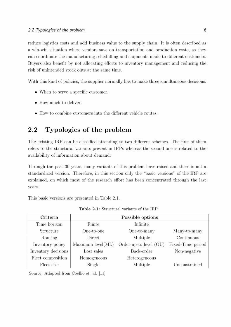
This basic versions are presented in Table 2.1.

Table 2.1: Structural variants of the IRP

Criteria Possible options

Time horizon Finite Infinite

Structure One-to-one One-to-many Many-to-many

Routing Direct Multiple Continuous

Inventory policy Maximum level(ML) Order-up-to level (OU) Fixed-Time period

Inventory decisions Lost sales Back-order Non-negative

Fleet composition Homogeneous Heterogeneous

Fleet size Single Multiple Unconstrained

Source: Adapted from Coelho et. al. [11]

2.2 Typologies of the problem 7

As it can be seen in the mentioned table, the models can be classified attending to seven

different criteria called: time horizon, structure, routing, inventory policy, inventory deci-

sions, fleet composition and fleet size.

In table 2.1, time refers to the horizon taken into account by the model which can be

either finite or infinite. The number of suppliers and customers can vary, and therefore the

structure of the IRP can be one-to-one when there is only one supplier and one customer,

one-to-many in the most common case having one supplier or depot that serves several

customers, or many-to-many with more than one suppliers and more than one customers.

Routing on the other side, can be direct when there is only one customer per route, multiple

when there are more than one customers clustered on the same route and continuous when

there is no central depot.

Inventory policies define pre-established rules to replenish customers. The two most com-

mon ones are the maximum level (ML) policy, the order-up-to-level (OU) and the Fixed-

Time Period policy. The order-up to level (OU) policy, determines the quantity shipped

to each retailer in such a way that the level of its inventory reaches a specific level smaller

than the retailer’s capacity. However, in the Maximum Level (ML) policy, the quantity

shipped to each retailer is such that the inventory cannot exceed its maximum level. Fi-

nally, in the Fixed-Time period policy, each customer is visited with fixed frequency and

is delivered different quantities of products each time.

Inventory decisions determine how inventory management is tackled. If this inventory is

allowed to be negative, then back-ordering occurs and the corresponding demand will be

served at a later stage. If there are no back-orders, then the extra demand is lost and is

considered as lost sales. In both cases there exist a penalty cost for the stock-out.

Finally, the last two criteria refer to fleet composition and size. The fleet can either be

homogeneous or heterogeneous and the maximum number of vehicles used can be fixed at

one single vehicle, limited at several vehicles or unconstrained.

The second classification criteria refers to the time at which information on demand be-

comes known. If it is constant and the information is fully available at the beginning of

the planning horizon, the problem is deterministic. If what is known is the probability dis-

tribution of demand, the problem is then stochastic and it yields the Stochastic Inventory

Routing Problem (SIRP)

2.3 Classification on the basic IRP 8

2.3 Classification on the basic IRP

In this master‘s dissertation, a unique distribution center is considered. It receives incoming

shipments when needed and then, it delivers to a set of customers already clustered in a

set of possible route options depending on their proximity and demand patterns. Demand

rates are considered constant and back ordering is not allowed. Therefore, this IRP is an

example of deterministic problem.

Attending to the first criteria scheme mentioned in the section 2.2, this Cyclic Inventory

Routing Problem can be described as follows:

• Firstly, the considered time horizon of this model is “Finite”, as the cycle of time

considered in the model is fixed despite it will be repeated continuously over time.

• Secondly, the structure of this model can be described as “One-to-many”, as only one

depot is considered from where products are delivered to a set of possible customers.

• In this model, several customers are clustered in a set of possible route options.

Therefore it can be classified as a “Multiple Routing” IRP.

• The inventory is managed with a “Fixed -Time period” policy for the first two versions

of this model as each customer is delivered with fixed periodic intervals and the order

size can fluctuate. However, the third version makes use of “Fixed-Order Quantity

Shipment” as it places the different orders when the inventory levels arrive to 0.

• Back-order and stock-out are not permitted. Therefore, the inventory levels are

“Non-negative”.

• Finally, the fleet is “Homogeneous” and its size is “Multiple” as a fixed number of

trucks are available.

Table 2.2: Classification on the basic versions of IRP

Reference Time Structure Routing Inventory Inventory Fleet Fleet size

horizon policy decisions com.

Fin

ite

Infinit

e

One-

to-o

ne

One-

to-m

any

Man

y-t

o-m

any

Dir

ect

Mult

iple

Con

tinuou

s

Max

imum

Lev

el

Ord

er-u

pto

leve

l

Per

iodic

Rev

iew

Los

tsa

les

Bac

klo

ggin

g

Non

-neg

ativ

e

Hom

ogen

eous

Het

erog

eneo

us

Sin

gle

Mult

iple

Unco

nst

rain

ed

Own project

Source: Adapted from Coelho et. al. [11]

2.4 Literature Review 9

2.4 Literature Review

Referring to the literature review, there are many papers that have had a notorious impact

on the development of this master dissertation.

First of all, the master thesis entitled “Coordinating inbound and outbound deliveries in a

distribution center’ M. Alsina, (2016) [4], has been taking into account in order to structure

some parts of this project. Actually, this last thesis has been born as a further application

of the abstract “Fleet optimization for cyclic inventory routing problems” B. Raa,(2014)

[3].

In B.Raa‘s (2014) [3] paper, an infinite horizon is considered, where the optimization of a

vehicle fleet is studied in order to periodically repeat a given set of routes considering the

overall cost rate that is composed of fixed vehicle costs, route-specific costs and holding

costs at the customers. The main difference with this paper is that B. Raa’s paper [3]

considers that the central depot has enough stock available to load all the shipments

during the time horizon and therefore, no coordination with inbound products is done.

In M.Alsina‘s (2016)[4] thesis, the mentioned consideration is removed and therefore, in-

bound deliveries are considered. Nevertheless, the customers are already clustered in a set

of pre-defined routes and therefore, the routes design phase is not considered. Moreover,

no inventory capacity is considered at the retailers. Finally, the different routes are unique

and have to be scheduled without the possibility of changing the routes to deliver the

different customers along time.

In the G. Iassinovskaia‘s (2017) paper [5], it is considered a producer, located at a depot,

who has to distribute his products to a set of customers. Moreover, each partner has a

storage area composed of both empty and loaded RTI stock, as characterized by initial

levels and maximum storage capacity. The idea of considering the inventory capacity of

each retailer has been extracted from this paper.

In the paper of Raa and Aghezzaf [12], a heuristic column generation approach is proposed,

analyzed and evaluated against a comparable state-of-the-art heuristic in order to solve an

inventory routing problem. In this paper, any stock-out is permitted and deterministic

customer demand rates are assumed, integrating vehicle fleet sizing, vehicle routing and

inventory management. Furthermore, some realistic constraints are introduced as in this

dissertation such as limited storage capacities or driving time restrictions .

2.4 Literature Review 10

The paper of B. Raa and W. Dullaert [13], has also been considered. The metaheuristic

proposed to solve the cyclic inventory routing problem has been used in order to design

the different route options of this thesis.

On the other hand, the paper of K. Shang et. al.,[6] and the one of M. Seifbarghy and M.

R. A. Jokar, [7] also consider a two-echelon system. Each facility faces Poisson independent

demands. Therefore, a stochastic is performed in order to obtain the optimal base-stock

levels and reorder intervals for all retailers.

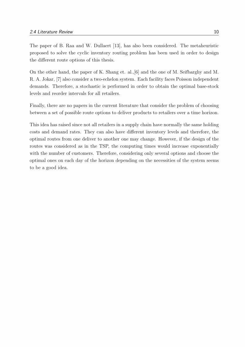
Finally, there are no papers in the current literature that consider the problem of choosing

between a set of possible route options to deliver products to retailers over a time horizon.

This idea has raised since not all retailers in a supply chain have normally the same holding

costs and demand rates. They can also have different inventory levels and therefore, the

optimal routes from one deliver to another one may change. However, if the design of the

routes was considered as in the TSP, the computing times would increase exponentially

with the number of customers. Therefore, considering only several options and choose the

optimal ones on each day of the horizon depending on the necessities of the system seems

to be a good idea.

MATHEMATICAL MODEL 11

Chapter 3

Mathematical model

This chapter explains the three different versions of the mathematical model developed

in this project as well as the notation used for data and variables as well as their main

differences.

3.1 Description of the problem

As this project is an enhancement of the “Fleet optimization for cyclic inventory rout-

ing problems” B. Raa, 2014 [3], and the master thesis of M. Alsina, 2016 [4], the same

framework of this papers has been used.

In this two-echelon supply chain system, the demand rates dj are set constant and the

considered time horizon is infinite. Therefore, the obtained schedule for a specific cycle,

must be repeated periodically. This cycle is established as the common multiple minimum

of the retailer‘s optimal cycle times.

Moreover, in this system, there is a depot in one stage, in which incoming and outgoing

deliveries must be coordinated and the transport of outgoing products to the retailers is

planned. As both parties are involved in the global cost of the supply chain, an integrated

supplier-retailer optimum will be achieved, which is more profitable than two separate

optimums.

3.1 Description of the problem 12

The considered retailers c ε C in this supply chain can be replenished from a set of possible

route options r ε R that have been created before-hand attending to proximity and cost

criteria. At each time-period, the model must choose between the different delivery options

in order to minimize the overall supply chain costs.

On the other hand, the required cycle time of each retailer is denoted by Tr. Each vehicle

has a limited truck capacity MM and each retailer has a limited storage capacity IKc.

Moreover, it takes a certain amount of time to complete a route Dr, including traveling

from the depot to the retailers, as well as the loading and unloading times of the vehicles

at the different places. A vehicle is also allowed to make several routes on one day, but the

total driving time per day is limited to M hours. It is therefore assumed that any route

cannot take more than this daily amount of time available (to avoid infeasibilities).

As the objective is to minimize the total costs, the cost structure must be defined. The

cost rate of the distribution schedule is composed out of the following four components:

• A fixed cost rate per vehicle F . The total number of vehicles that are available for

the distribution schedule is denoted by “V ”. When used, the cost rate per vehicle is

charged regardless its utilization, which means that even if one vehicle is only used

to make a small route with many days between consecutive iterations, the daily cost

is still charged for every day in the cycle.

• The cost for making the route r is denoted by Cr. This cost includes the cost of

loading the vehicles, transporting the items through the route and dispatching cost

at each retailer. It is worth mentioning that the cost of making each route is highly

dependent on the cost and duration of each route.

• The third component is the holding cost at each retailer and at the depot. In order

to compute this cost, a constant holding cost rate H per unit per day is charged at

both retailers and depot.

• The last component is the fixed cost for replenishing the depot S that is charged per

order each time the depot needs to receive incoming products.

3.2 Notation of parameters 13

Therefore, the cost of a distribution schedule in which a set of routes R is replenishing a

group of customers C is given by the following formula:

O.F. = Min∑

v ε V

F.nT.Zv +∑

r ε R

∑

v ε V

∑

d ε nT

XvrdCr +H.∑

d ε nT

IDd

+ H.∑

c ε C

∑

d ε nT

IRcd + S.∑

d ε nT

Yd(3.1)

The first term of the previous equation corresponds to the fixed vehicle cost of the vehicles

used in the distribution schedule. The second term is the cost of making the different

routes, while the third and fourth components of the same equation are the holding costs

at the depot and the retailers. Finally, the last component corresponds to the cost of

replenishing the depot.

3.2 Notation of parameters

The notation of the different parameters used in this project are listed below. At the same

time, a small explanation is given as well as its corresponding units:

R Number of possible route options to deliver the different retailers. Each route can

deliver either a unique retailer or more than one. A specific retailer can also be

delivered from more than one option.

C Number of retailers in the supply chain.

V Maximum number of outgoing delivery vehicles in a distribution schedule.

M Limit of total driving hours per day for each vehicle (h/day).

nT Total number of periods of the cycle (days).

Tc Periodicity of retailer “c” (days).

Dr Duration of route “r” (hours).

Demr Demand rate of retailer “c” (Number of units/day).

MM Truck capacity (Units).

Arc Binary matrix that indicates if the route “r” visits the retailer “c”.

3.3 Notation of variables 14

IKc Inventory capacity at the retailer “c”.

Cr Cost of making the route “r” (e/route).

F Fixed cost per vehicles in euros per day (e/day).

S Fixed cost for replenishing the depot (e/replenishment).

H Holding cost at the retailers and the depot (e/unit.day).

3.3 Notation of variables

The notation of the different variables are the listed below as well as a little explanation

of its notation.

Xvrd Binary variable that is “1” if the vehicle “v” makes the route “r” on day “’d’.

Zv Binary variable that indicates wether the vehicle “v” is used.

IDd Inventory level at the depot on day “’d’.

IRcd Inventory level at the retailer “c” on day “d”.

Yd Number of vehicles needed for replenishments of the depot on day “d”.

QId Number of units of product that enters the depot on day “d”.

QOrd Number of units of product that leave the depot through route “r” on day “d”.

Qdelrcd Number of units of product delivered through the route “r” to retailer “c” on day

“d”.

Sdelcd Total number of units delivered to retailer “c” on day “d” as sum of all the possible

options.

3.4 Mathematical model (Version 1) 15

3.4 Mathematical model (Version 1)

Once the notation has been established, the first mathematical model to solve this problem

can be developed.

As mentioned above. this version takes into account the periodicity requirements of each

retailer in order to deliver them every Tr days, making use of the same routes during each

delivery. Furthermore, the quantity delivered each time must be the same.

This model, schedules the routes in order to minimize the overall costs across the supply

chain within a finite space of time that will be repeated cyclically over the time.

The mathematical equations of the model are presented below. After the equations, a brief

explanation about each constraint is given.

O.F. = Min∑

v ε V

F.nT.Zv +∑

r ε R

∑

v ε V

∑

d ε nT

XvrdCr +H.∑

d ε nT

IDd

+ H.∑

c ε C

∑

d ε nT

IRcd + S.∑

d ε nT

Yd(3.2)

Zv ≤ Zv−1 ; ∀ v ε V (3.3)

ID0 = IDnT (3.4)

IRc0 = IRcnT ; ∀ c ε C (3.5)

IR10 = 0 (3.6)

IR11 ≥ IR1d ; ∀ d ε nT (3.7)

∑

v ε V

Qdelrcd ≤ MM∑

v ε V

Xvrd

{ ∀ d ε nT∀ r ε R (3.8)

Qdelrcd ≤ Ar cMM∑

v ε V

Xvrd

{ ∀ d ε nT∀ r ε R∀ c ε C

(3.9)

3.4 Mathematical model (Version 1) 16

QId ≤ MM Yd ; ∀ d ε nT (3.10)

IDd = IDd−1 +QId −∑

r ε R

∑

c ε C

Qdelrcd; ∀ d ε nT (3.11)

IRcd = IRcd−1 −Demc +∑

r ε R

Qdelrcd

{ ∀ d ε nT∀ c ε C (3.12)

IRcd ≤ IKc ; ∀c ε C (3.13)

Tc∑

d = 1

∑

v ε V

∑

r ε R

XvrdArc = 1 ; ∀ c ε C (3.14)

Qdelrcd = Qdelrcd+Tc −{ ∀ d ε nT − Tc∀ r ε R∀ c ε C

(3.15)

∑

r ε R

DrXvrd ≤ MZv

{ ∀ d ε nT∀ v ε V (3.16)

Sdelcd =∑

r ε R

Qdelrcd

{ ∀ c ε C∀ d ε nT (3.17)

Zv , Xvrd ε {0, 1} (3.18)

IDd , IRcd , Yd , QOrd , QId , Qdelrcd ; Sdelcd ≥ 0 (3.19)

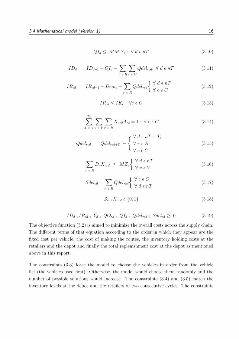
The objective function (3.2) is aimed to minimize the overall costs across the supply chain.

The different terms of that equation according to the order in which they appear are the

fixed cost per vehicle, the cost of making the routes, the inventory holding costs at the

retailers and the depot and finally the total replenishment cost at the depot as mentioned

above in this report.

The constraints (3.3) force the model to choose the vehicles in order from the vehicle

list (the vehicles used first). Otherwise, the model would choose them randomly and the

number of possible solutions would increase. The constraints (3.4) and (3.5) match the

inventory levels at the depot and the retailers of two consecutive cycles. The constraints

3.5 Periodic replenishment of retailers (Version 2) 17

(3.4) focus on the depot while the constraints (3.5) implement the same restriction for the

retailers.

The constraints (3.6) and (3.7) are set in order to break the symmetry of the solution by

fixing the inventory level at retailer 1 on day 0 equal to 0 and forcing that the highest ship-

ment to this retailer is made on the first day of the studied cycle. In this way, the number

of symmetric solutions is decreased and the running times are improved. Constraints (3.8)

force the total quantity delivered on one day to not exceed the capacity of the vehicles that

have been used. Constraints (3.9) force the quantity delivered to a specific retailer using

a route to be 0 if that route does not visit the retailer. Constraints (3.10) prevent the

quantity that enters the depot on day d ε nT from exceeding the vehicles capacity. Con-

straints (3.11) and (3.12) define the inventory at the depot and the retailers respectively.

Constraints (3.13) limit the inventory level at the retailers to not exceed their inventory

capacity. Constraints (3.14) ensure that it is only possible to visit a specific retailer one

time per cycle, with only one vehicle and using only one route. Constraints (3.15) ensure

that the quantity delivered to a retailer c ε C on a day d ε nT using a route r ε R is the

same after the periodic interval of that retailer Tc. Constraints (3.16) ensure that there

is no vehicle that exceeds the total driving time limit. Constraints (3.17) calculate the

total number of units delivered to a given customer c ε C through all the routes. Finally,

constraints (3.18) and (3.19) define the decision variables of the problem.

3.5 Periodic replenishment of retailers (Version 2)

In this section, a new mathematical version of the model is presented. Now, a periodic

schedule is assumed. However, the quantities delivered to each retailer and the routes

used to perform those shipments can vary on different days. The number of possible

solutions in this second version of the model increases respecting to the first model as the

quantities delivered to each retailer are not restricted to be regular and the routes can vary

. Furthermore, the optimal solution of the first model is included here. Hence, the solution

of this model can be the same or even better, but the execution time is increased as the

number of possible solutions also raises.

3.6 Non-periodic replenishment (Version 3) 18

The basis of this model is the same as in the last one. However, as the quantities delivered to

each customer does not have to be regular, the constraints (3.15) are replaced by constraints

(3.20).

∑

v ε V

∑

r ε R

XvrdArc =∑

v ε V

∑

r ε R

Xvrd+TcArc

{ ∀ c ε C∀ d ε nT − Tc

(3.20)

Equation 3.20 implies that one specific retailer c ε C has to be replenished with its required

periodicity Tc. However, it does not fix the route used to visit each retailer nor the vehicle

used. Therefore, either the quantity and the route used to visit a specific retailer can vary

from time to time.

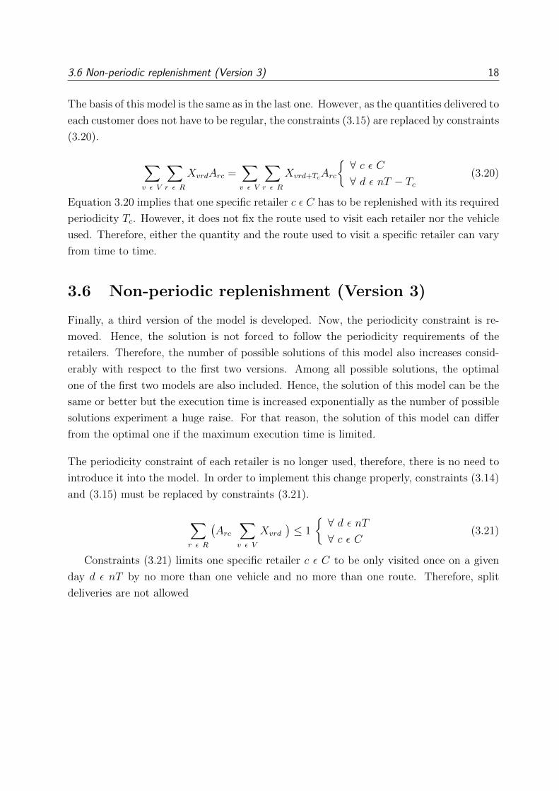
3.6 Non-periodic replenishment (Version 3)

Finally, a third version of the model is developed. Now, the periodicity constraint is re-

moved. Hence, the solution is not forced to follow the periodicity requirements of the

retailers. Therefore, the number of possible solutions of this model also increases consid-

erably with respect to the first two versions. Among all possible solutions, the optimal

one of the first two models are also included. Hence, the solution of this model can be the

same or better but the execution time is increased exponentially as the number of possible

solutions experiment a huge raise. For that reason, the solution of this model can differ

from the optimal one if the maximum execution time is limited.

The periodicity constraint of each retailer is no longer used, therefore, there is no need to

introduce it into the model. In order to implement this change properly, constraints (3.14)

and (3.15) must be replaced by constraints (3.21).

∑

r ε R

(Arc

∑

v ε V

Xvrd

)≤ 1

{ ∀ d ε nT∀ c ε C (3.21)

Constraints (3.21) limits one specific retailer c ε C to be only visited once on a given

day d ε nT by no more than one vehicle and no more than one route. Therefore, split

deliveries are not allowed

COMPUTATIONAL RESULTS 19

Chapter 4

Computational results

This section illustrates the behavior of our solution approach in two different ways. First,

the model is tested on a set of randomly generated problem instances. Next, this approach

is compared to the solution proposed by Raa and Dullaert [13] for the cyclic inventory

routing problem.

4.1 Design of instances

In the literature of the cyclic inventory routing problems, some datasets are available, e.g.

the paper of Sindhuchao et al., [8], the one of Aghezzaf et al., [9] or the paper of Birger

Raa [3].

However, these datasets cannot be used in this thesis for several reasons. In Sindhuchao

et al., [8], no fixed vehicle cost is considered; in Aghezzaf et al., [9], a single vehicle is

assumed so fleet sizing is not an issue; in Birger Raa [3], the route design phase is not

considered. Moreover, it does not take inventory capacity constraints at the retailers into

consideration.

However, due to similarities with this master thesis, the instances of this paper are based

on the instances proposed in Raa and Aghezzaf [12]. The mentioned instances have been

generated according to a 5 x 24 Factorial Design in which the different factors that have

been analyzed are illustrated in table 4.1.

4.1 Design of instances 20

The first factor is the customer storage capacity restriction (CCAP), with levels “No” and

“Yes” indicating if this restriction is taken into account or not. The second factor is the

holding cost rate (H), which can be either 8 or 80 eurocents per unit per day. This holding

cost factor (H) is assumed to be the same for all the customers and the depot. The third

factor is the Fixed Vehicle Cost (F), which can be either 100 and 400 euros per day. Finally,

the fourth and last factor is the number of customers (NR). The two levels that have been

considered for this factor are 10 and 15 customers.

Factor Shorthand Level Level

‘− 1′ ‘1′

Customer capacity CCAP No Yes

restriction

Holding cost rate H 0.08 e/ 0.8 e/

(u. day) (u. day)

Fixed Vehicle cost F 100 e/ 400 e/

(u. day) (u. day)

Number of customers NR 10 Cust. 15 Cust.

Table 4.1: Key factors considered in the Factorial Design

The test instances were introduced in Raa and Aghezzaf [12] are generated as follows. First,

the different retailers are located randomly within a service area circle. The radius of this

circle is randomly generated between 75 and 100 km and the depot is always placed in the

center of the circle. Euclidean distances are used. Customer demand rates are randomly

generated between 1 and 10 units per day. Furthermore, their customer storage capacity

is generated randomly such that it can hold between 2 and 10 days of supply.

Loading and dispatching the vehicles is assumed to take half an hour (tj=0.5 hour ∀j) and

cost 20 euro, while deliveries at the customers are assumed to take 15 minutes and cost

10 euro (tj = 0.25 hour ∀j). The vehicles have a capacity of 100 units, a vehicle speed

of 50 km per hour and a fixed vehicle cost that can be either 100 or 400 euro per day.

Furthermore, a variable cost of 1.2 euro per km is considered.

The total cost of each route option is composed out of the variable transportation cost of

each route multiplied by the length of each route, the loading and dispatching cost and

the delivery cost at each customer.


The duration of each route is calculated by taking into account the total length of the

route, considering a vehicle speed of 50 km/h and the dispatching time at the retailers as

well as the loading time at the depot (15 and 30 minutes respectively).

A fixed shipment cost of 35 euro per order is also charged to the incoming products at the

depot. The total driving time limit is 8 h and the maximum number of vehicles that can

be used is set to 5 and the considered time horizon is equal to 12 days.

Finally, 50 route options are considered for each of the instances. These options, have

been designed by making sub-tours of the optimal solutions provided by the algorithm

of Raa and Dullaert [13] for the same set of instances. In this way, a group of 50 good

solutions that contain the optimal ones are always taken into account for each instance.

Furthermore, the periodicity requirements of each customer have been extracted from this

solutions. The working principles of the heuristic algorithm developed in Raa and Dullaert

[13], are explained in appendix A.

The different models presented in this paper have been programmed with IBM ILOG

CPLEX Optimization Studio 12.7. Computational testing was done on a 2 GHz Intel(R)

Core (TM) i7-2630 QM with 4 GB of RAM limiting the maximum running time to 300

seconds.

The results for all 240 = (3 x 5 x 24) instances are summarized in tables 4.2, 4.3 and 4.4,

displaying the following solution characteristics, that will be used to explain the various

cost trade-offs and the way in which they are obtained:

• Total cost rate and its five different cost components;

• The maximum GAP of the solution after 300 seconds of running time;

• Number of vehicles used and number of tours;

• Utilization of the vehicle as the percentage of time that it is being used;

• Cumulative average stock level of all customers and depot;

• Average number of customers per tour.

After obtaining the mentioned results, it has been demonstrated that despite the fixed

vehicle cost F has an important effect on the total cost of the solution, it does not have

any real effect on the solutions.


Therefore, in order to evaluate the effects and the interactions of the different factors on the

total cost of the solution, a linear regression analysis is performed on each of the versions

of the model excluding the fixed vehicle cost factor F. Therefore, this analysis tests the

rest of the factors as well as their two-way interactions. Fig. 4.1 and fig. 4.2 show the

results of this analysis, provided by the statistical software R Studio 3.4.0.

CCAP H F NR Total Fleet Transport Depot Retailers Shipment GAP nr Veh nr Tours Utilization Stock Cust/tour

cost holding holding cost

cost cost

Yes 0,8 400 15 9.712,46 4.800,00 3.484,34 6,46 1.001,66 420,00 0,00% 1,00 3,80 67,94% 73,29 4,10

Yes 0,8 400 10 8.339,18 4.800,00 2.478,67 12,93 739,58 308,00 0,00% 1,00 3,20 47,75% 76,31 3,33

Yes 0,8 100 15 6.112,46 1.200,00 3.484,34 6,46 1.001,66 420,00 0,00% 1,00 3,80 67,94% 73,92 4,10

Yes 0,8 100 10 4.739,18 1.200,00 2.478,67 12,93 739,58 308,00 0,00% 1,00 3,20 47,75% 77,10 3,33

Yes 0,08 400 15 8.771,25 4.800,00 3.484,34 15,75 100,17 371,00 0,00% 1,00 3,80 67,94% 87,79 4,10

Yes 0,08 400 10 7.607,21 4.800,00 2.478,67 16,58 73,96 238,00 0,00% 1,00 3,20 47,87% 92,42 3,33

Yes 0,08 100 15 5.171,25 1.200,00 3.484,34 15,75 100,17 371,00 0,00% 1,00 3,80 67,94% 87,79 4,10

Yes 0,08 100 10 4.007,21 1.200,00 2.478,67 16,58 73,96 238,00 0,00% 1,00 3,20 47,75% 92,11 3,33

No 0,8 400 15 9.712,46 4.800,00 3.484,34 6,46 1.001,66 420,00 0,00% 1,00 3,80 67,94% 73,25 4,10

No 0,8 400 10 8.339,18 4.800,00 2.478,67 12,93 739,58 308,00 0,00% 1,00 3,20 47,75% 77,10 3,33

No 0,8 100 15 6.112,46 1.200,00 3.484,34 6,46 1.001,66 420,00 0,00% 1,00 3,80 67,94% 73,90 4,10

No 0,8 100 10 4.739,18 1.200,00 2.478,67 12,93 739,58 308,00 0,00% 1,00 3,20 47,75% 76,13 3,33

No 0,08 400 15 8.771,25 4.800,00 3.484,34 15,75 100,17 371,00 0,00% 1,00 3,80 67,94% 89,33 4,10

No 0,08 400 10 7.607,21 4.800,00 2.478,67 16,58 73,96 238,00 0,00% 1,00 3,20 47,87% 91,37 3,33

No 0,08 100 15 5.171,25 1.200,00 3.484,34 15,75 100,17 371,00 0,00% 1,00 3,80 67,94% 89,44 4,10

No 0,08 100 10 4.007,21 1.200,00 2.478,67 16,58 73,96 238,00 0,00% 1,00 3,20 47,75% 94,70 3,33

Table 4.2: Results for Model 1



cost cost

Yes 0,8 400 15 9.712,46 4.800,00 3.484,34 3,58 1.004,54 420,00 0,00% 1,00 3,80 67,94% 74,00 4,10

Yes 0,8 400 10 8.319,35 4.800,00 2.461,91 9,86 739,58 308,00 0,00% 1,00 3,20 47,75% 75,98 3,33

Yes 0,8 100 15 6.112,46 1.200,00 3.484,34 0,70 1.007,42 420,00 0,00% 1,00 3,80 67,94% 73,08 4,10

Yes 0,8 100 10 4.719,35 1.200,00 2.461,91 9,86 739,58 308,00 0,00% 1,00 3,20 47,75% 77,31 3,33

Yes 0,08 400 15 8.771,25 4.800,00 3.484,34 12,17 103,74 371,00 0,00% 1,00 3,80 67,94% 86,54 4,10

Yes 0,08 400 10 7.586,79 4.800,00 2.457,09 13,00 78,69 238,00 0,00% 1,00 3,20 47,75% 93,56 3,33

Yes 0,08 100 15 5.171,25 1.200,00 3.484,34 12,72 103,19 371,00 0,00% 1,00 3,80 67,94% 89,12 4,10

Yes 0,08 100 10 3.986,79 1.200,00 2.457,09 15,32 76,38 238,00 0,00% 1,00 3,20 47,75% 93,24 3,33

No 0,8 400 15 9.712,46 4.800,00 3.484,34 6,46 1.001,66 420,00 0,00% 1,00 3,80 67,94% 74,00 4,10

No 0,8 400 10 8.319,35 4.800,00 2.461,91 6,78 742,66 308,00 0,00% 1,00 3,20 47,75% 77,14 3,33

No 0,8 100 15 6.112,46 1.200,00 3.484,34 6,46 1.001,66 420,00 0,00% 1,00 3,80 67,94% 72,98 4,10

No 0,8 100 10 4.719,35 1.200,00 2.461,91 9,86 739,58 308,00 0,00% 1,00 3,20 47,75% 76,46 3,33

No 0,08 400 15 8.771,25 4.800,00 3.484,34 6,59 109,32 371,00 0,00% 1,00 3,80 67,94% 86,86 4,10

No 0,08 400 10 7.586,79 4.800,00 2.457,09 14,69 77,00 238,00 0,00% 1,00 3,20 47,75% 94,70 3,33

No 0,08 100 15 5.171,25 1.200,00 3.484,34 12,67 103,25 371,00 0,00% 1,00 3,80 67,94% 89,73 4,10

No 0,08 100 10 3.986,79 1.200,00 2.457,09 14,14 77,56 238,00 0,00% 1,00 3,20 47,75% 94,71 3,33

Table 4.3: Results for Model 2




cost cost

Yes 0,8 400 15 9.432,96 4.800,00 2.932,18 7,33 1.315,46 378,00 0,82% 1,00 6,80 57,57% 93,16 2,36

Yes 0,8 400 10 7.957,28 4.800,00 2.081,11 9,86 793,31 273,00 0,25% 1,00 4,60 40,38% 76,22 2,33

Yes 0,8 100 15 5.833,52 1.200,00 2.919,27 7,49 1.321,76 385,00 1,57% 1,00 6,80 57,38% 93,24 2,34

Yes 0,8 100 10 4.359,72 1.200,00 2.085,09 10,24 791,39 273,00 1,56% 1,00 4,80 39,98% 82,14 2,23

Yes 0,08 400 15 8.089,31 4.800,00 2.741,97 3,94 172,40 371,00 0,13% 1,00 7,20 53,70% 129,90 2,12

Yes 0,08 400 10 7.116,48 4.800,00 1.958,24 6,63 113,61 238,00 0,08% 1,00 6,00 40,94% 123,43 1,81

Yes 0,08 100 15 4.490,82 1.200,00 2.741,97 5,13 172,73 371,00 0,47% 1,00 7,40 53,70% 130,59 2,07

Yes 0,08 100 10 3.517,19 1.200,00 1.958,24 7,97 112,98 238,00 0,69% 1,00 6,00 37,71% 124,33 1,81

No 0,8 400 15 9.321,51 4.800,00 2.583,54 5,22 1.554,75 378,00 1,83% 1,00 7,20 50,89% 110,49 2,33

No 0,8 400 10 7.668,54 4.800,00 1.633,11 3,58 979,84 252,00 1,23% 1,00 5,40 32,15% 99,22 1,92

No 0,8 100 15 5.724,24 1.200,00 2.597,64 4,03 1.537,57 385,00 6,13% 1,00 6,80 51,14% 107,65 2,45

No 0,8 100 10 4.061,31 1.200,00 1.567,51 5,86 1.042,94 245,00 6,52% 1,00 5,60 30,91% 106,92 1,80

No 0,08 400 15 7.486,97 4.800,00 1.963,14 0,71 352,12 371,00 1,64% 1,00 11,20 38,18% 251,74 1,35

No 0,08 400 10 6.400,54 4.800,00 1.158,61 0,00 203,93 238,00 0,85% 1,00 6,40 32,30% 211,59 1,65

No 0,08 100 15 3.889,77 1.200,00 1.960,24 2,28 356,25 371,00 3,75% 1,00 11,20 38,11% 253,58 1,35

No 0,08 100 10 3.016,81 1.200,00 1.383,81 1,29 193,72 238,00 1,44% 1,00 6,20 26,70% 200,71 1,67

Table 4.4: Results for model 3


(a) Model 1 (b) Model 2

(c) Model 3

Figure 4.1: Output from the linear regression analysis for the total cost rate taking into account

the two-interaction analysis


(a) Model 1 (b) Model 2

(c) Model 3

Figure 4.2: Output from the linear regression analysis for the total cost rate taking into single

influence of each factor

The results of the mentioned analysis show that any of the two-way interactions have a

significant effect on the solution for any of the three different models. Furthermore, the

customer storage capacities are not significant for any of the first two versions but have a

significant effect on the third one. The rest of the factors have all a significant influence

on the final solutions.

4.2 Effect of the customer storage capacity restriction 26

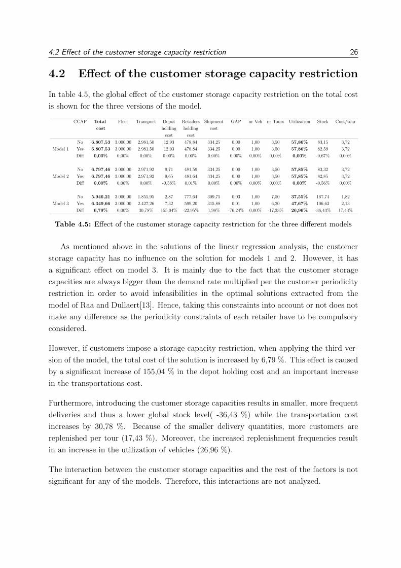
4.2 Effect of the customer storage capacity restriction

In table 4.5, the global effect of the customer storage capacity restriction on the total cost

is shown for the three versions of the model.

CCAP Total Fleet Transport Depot Retailers Shipment GAP nr Veh nr Tours Utilization Stock Cust/tour


cost cost

Model 1

No 6.807,53 3.000,00 2.981,50 12,93 478,84 334,25 0,00 1,00 3,50 57,86% 83,15 3,72

Yes 6.807,53 3.000,00 2.981,50 12,93 478,84 334,25 0,00 1,00 3,50 57,86% 82,59 3,72

Diff 0,00% 0,00% 0,00% 0,00% 0,00% 0,00% 0,00% 0,00% 0,00% 0,00% -0,67% 0,00%

Model 2

No 6.797,46 3.000,00 2.971,92 9,71 481,59 334,25 0,00 1,00 3,50 57,85% 83,32 3,72

Yes 6.797,46 3.000,00 2.971,92 9,65 481,64 334,25 0,00 1,00 3,50 57,85% 82,85 3,72

Diff 0,00% 0,00% 0,00% -0,58% 0,01% 0,00% 0,00% 0,00% 0,00% 0,00% -0,56% 0,00%

Model 3

No 5.946,21 3.000,00 1.855,95 2,87 777,64 309,75 0,03 1,00 7,50 37,55% 167,74 1,82

Yes 6.349,66 3.000,00 2.427,26 7,32 599,20 315,88 0,01 1,00 6,20 47,67% 106,63 2,13

Diff 6,79% 0,00% 30,78% 155,04% -22,95% 1,98% -76,24% 0,00% -17,33% 26,96% -36,43% 17,43%

Table 4.5: Effect of the customer storage capacity restriction for the three different models

As mentioned above in the solutions of the linear regression analysis, the customer

storage capacity has no influence on the solution for models 1 and 2. However, it has

a significant effect on model 3. It is mainly due to the fact that the customer storage

capacities are always bigger than the demand rate multiplied per the customer periodicity

restriction in order to avoid infeasibilities in the optimal solutions extracted from the

model of Raa and Dullaert[13]. Hence, taking this constraints into account or not does not

make any difference as the periodicity constraints of each retailer have to be compulsory

considered.

However, if customers impose a storage capacity restriction, when applying the third ver-

sion of the model, the total cost of the solution is increased by 6,79 %. This effect is caused

by a significant increase of 155,04 % in the depot holding cost and an important increase

in the transportations cost.

Furthermore, introducing the customer storage capacities results in smaller, more frequent

deliveries and thus a lower global stock level( -36,43 %) while the transportation cost

increases by 30,78 %. Because of the smaller delivery quantities, more customers are

replenished per tour (17,43 %). Moreover, the increased replenishment frequencies result

in an increase in the utilization of vehicles (26,96 %).

The interaction between the customer storage capacities and the rest of the factors is not

significant for any of the models. Therefore, this interactions are not analyzed.

4.3 Effect of the holding cost rate 27

4.3 Effect of the holding cost rate

In table 4.3, the global effect of the holding cost rate on the total cost is shown for the

three different versions of the model.

H Total Fleet Transport Depot Retailers Shipment GAP nr Veh nr Tours Utilization Stock Cust/tour


cost cost

Model 1

0,8 7.225,82 3.000,00 2.981,50 9,70 870,62 364,00 0,00 1,00 3,50 57,85% 75,12 3,72

0,08 6.389,23 3.000,00 2.981,50 16,17 87,06 304,50 0,00 1,00 3,50 57,88% 90,62 3,72

Diff -11,58% 0,00% 0,00% 66,73% -90,00% -16,35% 0,00% 0,00% 0,00% 0,05% 20,63% 0,00%

Model 2

0,8 7.215,91 3.000,00 2.973,12 6,70 872,09 364,00 0,00 1,00 3,50 57,85% 75,12 3,72

0,08 6.379,02 3.000,00 2.970,71 12,66 91,14 304,50 0,00 1,00 3,50 57,85% 91,06 3,72

Diff -11,60% 0,00% -0,08% 89,13% -89,55% -16,35% 0,00% 0,00% 0,00% 0,00% 21,22% 0,00%

Model 3

0,8 6.794,88 3.000,00 2.299,93 6,70 1.167,13 321,13 0,02 1,00 6,00 45,05% 96,13 2,22

0,08 5.500,99 3.000,00 1.983,28 3,49 209,72 304,50 0,01 1,00 7,70 40,17% 178,23 1,73

Diff -19,04% 0,00% -13,77% -47,85% -82,03% -5,18% -54,52% 0,00% 28,33% -10,84% 85,41% -22,11%

Table 4.6: Effect of the holding cost rate for the three different models

The holding cost rate has a notorious impact on the total overall cost of the solutions for

the three different algorithms. Moreover, the results of the linear regression test show that

this factor has a significant influence on the solutions for the three models. However, its

two-way interactions are not significant and therefore, will not be analyzed.

When changing from high holding costs to low holding costs but no other factors are

changed, the total cost decreases by 11,58 % for model 1, 11,60 % for model 2 and 19,04

% for model 3.

Furthermore, when holding costs are low, larger deliveries are made. There is indeed an

increase of 20,63 % in the global stock level for model 1, an increase of 21,22 % for model

2 and an increase of 85,41 % for model 3.

The larger delivery quantities imply that for model 3 less customers are visited per tour

(22,11 %) and it does not have any effect for the other two models. Finally, deliveries are

also made less frequent. As a result, transportation costs does not change for model 1, but

decrease by 0,08 % for model 2 and by 13,77 % for model 3.

4.4 Effect of the number of customers 28

4.4 Effect of the number of customers

In table 4.7, the global effect of the number of customers on the overall cost for the three

models of this paper is illustrated.

NR Total Fleet Transport Depot Retailers Shipment GAP nr Veh nr Tours Utilization Stock Cust/tour


cost cost

Model 1

10 6.173,20 3.000,00 2.478,67 14,76 406,77 273,00 0,00 1,00 3,20 47,78% 84,65 3,33

15 7.441,86 3.000,00 3.484,34 11,11 550,92 395,50 0,00 1,00 3,80 67,94% 81,09 4,10

Diff 20,55% 0,00% 40,57% -24,72% 35,44% 44,87% 0,00% 0,00% 18,75% 20,16 % -4,21% 23,00%

Model 2

10 6.153,07 3.000,00 2.459,50 11,69 408,88 273,00 0,00 1,00 3,20 47,75% 85,39 3,33

15 7.441,86 3.000,00 3.484,34 7,67 554,35 395,50 0,00 1,00 3,80 67,94% 80,79 4,10

Diff 20,95% 0,00% 41,67% -34,37% 35,58% 44,87% 0,00% 0,00% 18,75% 20,19% -5,39% 23,00%

Model 3

10 5.512,23 3.000,00 1.728,22 5,68 528,96 249,38 0,02 1,00 5,63 35,14% 128,07 1,90

15 6.783,64 3.000,00 2.554,99 4,52 847,88 376,25 0,02 1,00 8,08 50,08% 146,29 2,05

Diff 23,07% 0,00% 47,84% -20,46% 60,29% 50,88% 0,00% 0,00% 43,56% 14,95% 14,23% 7,48%

Table 4.7: Effect of the number of customers

As table 4.7 shows, there exist a small economy of scale when servicing customers. The

total cost increases by around 20 % when the number of customers increases by 50 % in the

three different models. Moreover, the cost trade-off being made is different for small and

large instances. In large instances, more customers are served per tour while at the same

time larger quantities are delivered. This seems contradictory but it is possible because of

the increased utilization of the vehicles.

The interaction between the number of customers and the rest of the considered factors does

not have a significant influence on the solutions and therefore, they will not be analyzed.

4.5 Comparison to another heuristic 29

4.5 Comparison to another heuristic

In this section, the three different models developed in this paper are compared with an

metaheuristic algorithm on a specific set of instances.

Raa and Dullaert [13] presented in 2017 this metaheuristic approach for the cyclic inventory

routing problem under constant customer demand rates. In this framework, they made

some simplifying assumptions such as not allowing split delivery or imposing a constant

time between consecutive deliveries.

As in most of the papers found in the literature on cyclic inventory routing problems, the

incoming products to the depot are not considered and thus, neither the holding cost at

this depot. As a result, the coordination of inbound products is not considered in the

solution of Raa and Dullaert [13]. For the routes design, each of the several customers are

grouped in a tour with specific tour frequencies and cycle times. This means that, one

customer which has been inserted into a specific tour will always receive the product with

the cycle time of that specific tour even if it is not the optimal cycle time for that specific

customer on a given day.

To compare our solution approach to that of Raa and Dullaert, the fixed shipment cost

(S = 0) and the holding cost at the depot (Hd = 0) have been ignored .

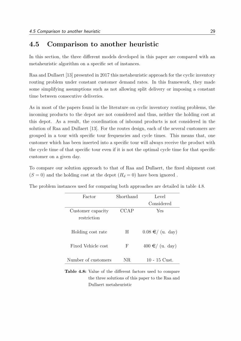
The problem instances used for comparing both approaches are detailed in table 4.8.

Factor Shorthand Level

Considered

Customer capacity CCAP Yes

restriction

Holding cost rate H 0.08 e/ (u. day)

Fixed Vehicle cost F 400 e/ (u. day)

Number of customers NR 10 - 15 Cust.

Table 4.8: Value of the different factors used to compare

the three solutions of this paper to the Raa and

Dullaert metaheuristic

4.5 Comparison to another heuristic 30

In table 4.9, the results of the three different models developed in this thesis are listed

in comparison to the Raa and Dullaert heuristic results for each of the instances. The

different cost rates are expressed in e/day.

For all problem instances, solutions are found that are cheaper that those proposed by Raa

and Dullaert [13]. It is worth mentioning that the cost decrease for the first two versions

of the model is not significant (On average less than 1 for low instances%).

However, for the third version of the model, this cost decrease is on average 4,93 % for

small instances and 10,34 % for large instances. This significantly better behavior is mostly

due to the more freedom in the development of tours for the third version of this model.

In table 4.10, the different components of the total cost rates are expressed in detail.

CCAP F H NR Raa and Dullaert Ver. 1 ∆ Ver. 2 ∆ Ver. 3 ∆

Yes 400 8c 10 615,2626 612,72 -0,41% 610,92 -0,71% 584,93 -4,93%

Yes 400 8c 15 716,6962 698,71 -2,51% 698,71 -2,51% 642,59 -10,34%

Table 4.9: Comparing the solution characteristics

These results show that taking into account many tour possibilities instead of one

specific tour possibility to serve each customer, gives the opportunity to use the vehicles

capacity much more efficiently and find much better cost trade-offs.

Total Cost Fixed veh. cost Transportation Cost Holding Cost Ret CPU-Time (s) nr veh nr tour Cust/tour

B. Raa/W. Dullaert 665,98 400,00 255,99 9,99 10,01 1,0 3,5 3,72

Version 1 655,71 400,00 248,46 7,26 8,08 1,0 3,5 3,72

diff -1,54% 0,00% -2,94% -27,36% -19,25% 0,00% 0,00% 0,00%

Version 2 654,81 400,00 247,56 7,26 7,65 1,0 3,5 3,72

diff -1,68% 0,00% -3,29% -27,36% -23,57% 0,00% 0,00% 0,00%

Version 3 613,76 400,00 202,22 11,54 267,78 1,0 6,9 1,88

diff -7,84% 0,00% -21,01% 15,58% 2576,54% 0,00% 97,14% -49,43%

Table 4.10: Comparing the solution characteristics

Despite the better results in the solutions for model 3, the running times are on average

267,78 seconds, while the running times for the model of Raa and Dullaert are on average

10 seconds. It is an evidence of slow performance which should be improved by creating a

heuristic in order to extend the scope of this problem to real instances.

CONCLUSIONS 31

Chapter 5

Conclusions

In this section, a set of technical and personal considerations are given. These conclusions

have been extracted after analyzing the three different mathematical algorithms developed

in this master dissertation and understanding the behavior of this models.

5.1 Technical outcomes

First of all, this paper analyses a cyclic planning approach for a two-echelon inventory

system. In addition, a first mathematical model optimizes the fleet vehicle size according

to the costs involved and the trade-off between the rest of expenses.

In this model, the vehicle fleet is used for periodic replenishments taking into account the

optimal cycle time of each route with regular quantities. A second mathematical model

with irregular quantities is presented. Finally, a third non-periodic model is developed in

order to see if there exists any worth improvement in increasing the number of possible

solutions by removing the periodicity constraints at the retailers. This assumption revealed

that some deliveries should be performed with a non-periodic frequency and irregular

quantities in order to achieve a notorious cost decrease.

A 3 x 5 x 24 factorial design of experiments is repeated for both periodic and non-periodic

models. Two levels were defined for each of the four presented factors (Customer storage

capacity restrictions, number of customers, fixed vehicle cost and holding cost rate).

5.1 Technical outcomes 32

The results of this experiments have been analyzed and some factors were noticed to

influence more than others in the schedule resolution:

• The first studied factor is the customer storage capacity restrictions with the levels

“Yes” or “No”. It has been noticed that this kind of restrictions are not significant

for any of the two first models. However, it has been noticed a significant effect on

the third model where the total cost of the solution is increased by 6,79 % when

applying these restrictions. Moreover, introducing the customer storage capacities

results in smaller, more frequent deliveries, causing a lower global stock level and an

increase in the transportation costs. These smaller delivery quantities also cause an

increased utilization of the vehicles and more customers visited per tour.

• Secondly, the holding cost rate was analyzed. In this case, the holding cost has a

notorious influence on the total cost for the three different models. Furthermore,

when holding costs are low, larger deliveries are performed causing a significant in-

crease on the average stock level. These larger delivery quantities also imply that

less customers are visited per tour.

• The last considered factor is the number of customers. It has been noticed that

there is a small economy of scale when servicing customers. Moreover, in larger

instances, more customers are served per tour while at the same time larger quantities

are delivered. This seems contradictory but it is possible because of the increased

utilization of the vehicles.

• Finally, the two-way interactions of this factors are not significant and therefore have

not been analyzed

Despite the character of this abstract, further applications can arise from the model and

a personalization of them can be performed. More constraints can be added such as

warehouse capacities, driving regulations or time windows for deliveries. However, they

have not been implemented as the objective of this paper is to analyze how the transport

costs are spread through the considered cycle time and it does not add significant value to

this analysis.

5.2 Suggestions for further research 33

5.2 Suggestions for further research

In this problem, several delivery options to visit the different customers, are considered.

For the problem instances of this dissertation, they have been made by randomly creating

subtours of the optimal solutions provided by the Raa and Dullaert algorithm [13] . One

interesting improvement would be the design of a heuristic algorithm to find 50 good

delivery options which contains the optimal solutions for each period in different situations

more efficiently.

Another interesting improvement since the version 3 of this dissertation provides really

good results compared to another existing algorithms but has excessive running times for

real instances, would be the development of a heuristic that finds near-optimal solutions

in smaller running times. Therefore, this solution could be applied to real instances more

easily.

5.3 Personal outcomes

The objective of this master‘s dissertation was to find a solution for a specific cyclic in-

ventory routing problem. In this particular case, a big scenario was decomposed in many

little goals easy to fix.

For me, the most difficult part was the analysis of the solutions of the different problem

instances and the process of extracting conclusions from them. It is not always easy to

interpret the reasons of a specific behavior in the models when changing one key factor.

However, I am glad to overcome that challenge. I take with me a large number of new

cross skills and competences learned while carrying out this project as well as the desire

to continue with this research in the future.

REFERENCES 34

References

[1] R. Handfield and K. P. McCormack, Supply chain risk management: minimizing dis-

ruptions in global sourcing. CRC press, 2007.

[2] S. Chopra and P. Meindl, Supply chain management-Strategy, Planning and Operation.

Pearson Education, third ed., 2006.

[3] B. Raa, “Fleet optimization for cyclic inventory routing problems,” International Jour-

nal of Production Economics, vol. 160, pp. 172–181, 2015.

[4] M. Alsina Marti, “Coordinating inbound and outbound deliveries in a distribution

center,” 2016.

[5] G. Iassinovskaia, S. Limbourg, and F. Riane, “The inventory-routing problem of re-

turnable transport items with time windows and simultaneous pickup and delivery in

closed-loop supply chains,” International Journal of Production Economics, vol. 183,

pp. 570–582, 2017.

[6] K. H. Shang, Z. Tao, and S. X. Zhou, “Optimizing reorder intervals for two-echelon

distribution systems with stochastic demand,” Operations Research, vol. 63, no. 2,

pp. 458–475, 2015.

[7] M. Seifbarghy and M. R. A. Jokar, “Cost evaluation of a two-echelon inventory system

with lost sales and approximately poisson demand,” International journal of produc-

tion economics, vol. 102, no. 2, pp. 244–254, 2006.

[8] S. Sindhuchao, H. E. Romeijn, E. Akcali, and R. Boondiskulchok, “An integrated

inventory-routing system for multi-item joint replenishment with limited vehicle ca-

pacity,” Journal of Global Optimization, vol. 32, no. 1, pp. 93–118, 2005.

[9] E.-H. Aghezzaf, Y. Zhong, B. Raa, and M. Mateo, “Analysis of the single-vehicle

cyclic inventory routing problem,” International Journal of Systems Science, vol. 43,

no. 11, pp. 2040–2049, 2012.

REFERENCES 35

[10] H. Andersson, A. Hoff, M. Christiansen, G. Hasle, and A. Løkketangen, “Industrial

aspects and literature survey: Combined inventory management and routing,” Com-

puters & Operations Research, vol. 37, no. 9, pp. 1515–1536, 2010.

[11] L. C. Coelho, J.-F. Cordeau, and G. Laporte, “Thirty years of inventory routing,”

Transportation Science, vol. 48, no. 1, pp. 1–19, 2013.

[12] B. Raa and E.-H. Aghezzaf, “A practical solution approach for the cyclic inventory

routing problem,” European Journal of Operational Research, vol. 192, no. 2, pp. 429–

441, 2009.

[13] B. Raa and W. Dullaert, “Route and fleet design for cyclic inventory routing,” Euro-

pean Journal of Operational Research, vol. 256, no. 2, pp. 404–411, 2017.

[14] “Council of Supply Chain Management Professionals.” https://cscmp.org/. Ac-

cessed: 27-04-2017.

[15] A. Fisher, “Wanted: 1.4 million new supply chain workers by 2018.” http://fortune.

com/2014/05/01/wanted-1-4-million-new-supply-chain-workers-by-2018/.

Accessed: 09-05-2017.

https://cscmp.org/

http://fortune.com/2014/05/01/wanted-1-4-million-new-supply-chain-workers-by-2018/

http://fortune.com/2014/05/01/wanted-1-4-million-new-supply-chain-workers-by-2018/

METAHEURISTIC APPROACH FOR THE DESIGN OF DELIVERY OPTIONS 36

Appendix A

Metaheuristic approach for the

design of delivery options

In this section, the metaheuristic approach in which this paper is based for the design of

the 50 different delivery options to each retailer will be explained in detail. This algorithm

was published in 2017 by Raa and Dullaert [13].

This metaheuristic is composed out of three different building blocks: the route design

subproblem, the fleet design subproblem and finally, a metaheuristic framework that is

built around these elements.

A.1 Route design phase

In this first phase of the algorithm, cyclic routes are designed in such a way that customer

sequencing minimize the travel distance and costs. Furthermore, the cycle time has to be

determined by trading-off the costs of making the route and the inventory holding costs

at the customers. This cycle time is also constrained by the vehicles capacity and the

customers storage capacities.

Suppose a set S of customers to be replenished and that route r visits a subset of these

customers Sr. Every customer i ε Sr has a constant demand rate di and a storage capacity

of ki units. Furthermore, a truck with a capacity of k units is available for making the

route from which the cycle time Tr has to be determined.

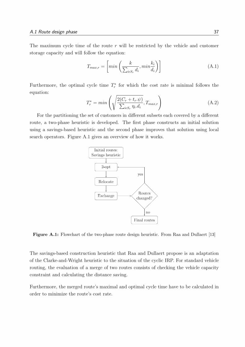
A.1 Route design phase 37

The maximum cycle time of the route r will be restricted by the vehicle and customer

storage capacity and will follow the equation:

Tmax,r =

[min

(k∑iεSr

di,min

kidi

)](A.1)

Furthermore, the optimal cycle time T ∗r for which the cost rate is minimal follows the

equation:

T ∗r = min

(√2(Cr + tr.ψ)∑

iεSrηi.di

, Tmax,r

)(A.2)

For the partitioning the set of customers in different subsets each covered by a different

route, a two-phase heuristic is developed. The first phase constructs an initial solution

using a savings-based heuristic and the second phase improves that solution using local

search operators. Figure A.1 gives an overview of how it works.

Figure A.1: Flowchart of the two-phase route design heuristic. From Raa and Dullaert [13]

The savings-based construction heuristic that Raa and Dullaert propose is an adaptation

of the Clarke-and-Wright heuristic to the situation of the cyclic IRP. For standard vehicle

routing, the evaluation of a merge of two routes consists of checking the vehicle capacity

constraint and calculating the distance saving.

Furthermore, the merged route’s maximal and optimal cycle time have to be calculated in

order to minimize the route’s cost rate.

A.2 Fleet design 38

The second phase of the route design is a local search based improvement phase. The local

search procedure can be considered as a variable neighborhood descent algorithm (VND),

consisting of various well-known algorithms.

In this second phase, the following standard local search operators are being used:

1. 2-Opt: Remove two arcs and replace them by two other arcs such that no subtours

are formed and all routes are closed again.

2. Relocate: Remove a customer and try to reinsert it into another position.

3. Exchange: Switch the position of two customers from either the same or different

routes.

As shown in figure A.1, the same local search operator is reiterated until no further im-

provements are achieved before moving on to the next operator.

Further, a modified best-accept strategy per operator is adopted in which nodes affected

by a move, are marked as affected in order to achieve a better computational efficiency.

A.2 Fleet design

When a set of cyclic routes is selected, the solution for all of them is also cyclic with a

cycle time equal to the least common multiple of all the individual route cycle times. To

limit this least common multiple, route cycle times are limited to T = 120 days and all

its divisors. However, in the solutions obtained for the design of the different delivery

options of this dissertation, this cycle times are limited to 12 days and all its divisors i.e.

{1,2,3,4,6,12}. In doing so, the infinite horizon is limited to a horizon of 12 days and the

same solution will be repeated cyclically.

The second step is to build a schedule within this horizon that indicates which vehicle

makes each route, taking into account that there shouldn’t be any vehicle that exceeds the

total driving limit of time H (e.g. 8 hours) and such that the sum of the cost rates and

the vehicle cost rate is minimized.

A.2 Fleet design 39

During this fleet design phase, better solutions can often be obtained if the individual route

cycle times are modified in order to align route cycle times to reduce the required fleet size.

However, deviating from the optimal route cycle times will increase the individual route

cost rates and is therefore only justified if that cost rate increase does not exceed the saving

of reducing the fleet. Thus, in this phase, the composition of the routes is not changed,

but their cycle times can still be adjusted to minimize the required fleet.

If a route r is made on day t , then it is also made on days t+ Tr,t+ 2 Tr, etc. Thus, the

cycle time Tr has to be selected along with a day t in the first Tr days of the schedule for

each route. Then, for all days t+ kTr,∀k ε{0, 1, ... TTr − 1}, a vehicle must be selected that

has enough time left to make the route on that day.

At this point, the fleet design subproblem makes use of the algorithm proposed by Raa in

2015 [3] which consists of two phases: a construction and an improvement phase.

Figure A.2: Flowchart of the two-phase fleet design heuristic. From Raa and Dullaert [13]

The construction heuristic is a best-fit insertion heuristic in which each route is inserted

in the way that the cumulative remaining time of the vehicles to which the routes are

assigned is minimal.

A.3 Metauristic framework 40

Within the construction heuristic, two cycle time selection rules are used. One where routes

are inserted with cycle times as close as possible to their optimal cycle times, and another

one where routes are inserted with cycle times as close as possible to their maximal cycle

times to minimize the fleet cost rate.

This leads to two initial schedules that are subsequently passed on to the improvement

step which consists of two local-search operators:

1. Remove and reinsert any single route in the cheapest possible way.

2. Remove all routes made by the vehicle with the lowest utilization and reinsert them

in the cheapest possible way.

To escape the local optimum, the schedule is scrambled by shuffling route allocations among

the vehicles according to a random permutation for every day in the schedule horizon. The

stopping criterion is a predefined number of scrambles.

Figure A.2 gives an overview on how the fleet design phase works. Further details on this

algorithm can be found in the paper of B. Raa [3]

A.3 Metauristic framework

With some adjustments, the algorithm of the fleet design phase is reused as the building

blocks in a metaheuristic framework that generates multiple solutions and retains the best

ones.

The first adjustment to the savings heuristic is made when two routes p and q are merged

into a single route and the savings are calculated as follows: Spq = TCRp + TCRq −λ. Varying the parameter λ leads to different solutions. This metaheuristic varies this

parameter between 0.8 and 1.5.

A second adjustment to lead the heuristic to different solutions is when parameterizing the

utilization in the computation of the total cost rate:

TCRr =CrTr

+Tr2

∑

iεSr

ηidi + αtrTrψ (A.3)

The parameter α represents the relative importance of the vehicle utilization versus the

actual route costs and is randomized with its value ranging between 0 and 2.

A.3 Metauristic framework 41

The first framework generates different solutions by randomizing the parameters α and λ.

A second framework is a ruin-and-recreate heuristic that iteratively destroys and rebuilds

a given solution. Ruining is done by iteratively removing a random number of customers

while recreation is carried out by applying the route and fleet design heuristics to the

partial solution.

In the third and final framework, the ruin-and-recreate heuristic is also adopted. It is

referred as “memetic algorithm” (MA).

This MA lies in the fact that it only uses the basic building blocks mentioned above and

it does not require complicated chromosome encodings.

The crossover operator used in this MA also works in a ruin-and-recreate manner. An

offspring solution is generated by removing a random number of customers from one of

the parent solutions, not only customers which are not incident to common arcs in both

parents can be removed. The resulting partial solutions after removing some customers

are optimized again using the route and fleet design heuristics outlined before.

Finally, another operator choice is population management. The population management

is used to take care of the diversification of the search process, this is done by measuring

the diversity of the individuals in the population and selecting individuals for crossover

with the well-known roulette wheel mechanism based on these diversity scores. Further,

the diversity scores are also used in composing the next generation of the population. This

next generation is composed of the best solutions from the population and the most diverse

among the offspring.

For further details, I refer to Raa and Dullaert (2017) [13]

TABLE ANNEX 42

Appendix B

Table annex

In the following page, a table with the different numerical results for all of the different

instances is attached.

Moreover, some calculations like the utilization of the vehicles, the number of vehicles per

tour and the average cumulative stock level at the customers and depot are performed.

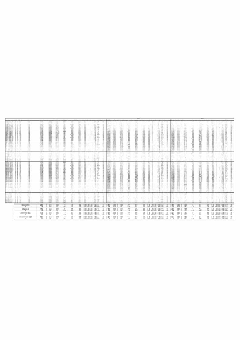
Dataset nr cust IK C F H Total Cost Fixed Vehicle cost Transportation cost Depot Holding cost Retailers holding cost Fixed Incoming cost GAP nr Veh nr Tours Utilization Stock nr customers/tour Total Cost Fixed Vehile cost Transportation cost Depot Holding cost Retailers holding cost Fixed Incoming cost GAP nr veh nr tours Utilization Stock nr customers/tour Total Cost Fixed Vehile cost Transportation cost Depot Holding cost Retailers holding cost Fixed Incoming cost GAP nr veh nr tours Utilization Stock nr customer/tour

CCAPyes_NRl_Hh_Fh_0 10 Yes 10 400 0,80 9.103,36 € 4.800,00 € 3.310,72 € 64,64 € 648,00 € 280,00 € 0,00% 1 4 62,51% 72,34 2,50 9.004,19 € 4.800,00 € 3.226,91 € 49,28 € 648,00 € 280,00 € 0,00% 1 4 62,51% 68,91 2,50 8.458,85 € 4.800,00 € 2.544,41 € 49,28 € 820,16 € 245,00 € 0,88% 1 6 48,69% 72,34 1,67



CCAPyes_NRl_Hh_Fh_3 10 Yes 10 400 0,80 8.555,33 € 4.800,00 € 2.226,45 € 0,00 € 1.178,88 € 350,00 € 0,00% 1 4 42,73% 120,91 2,50 8.555,33 € 4.800,00 € 2.226,45 € 0,00 € 1.178,88 € 350,00 € 0,00% 1 4 42,73% 122,75 2,50 8.417,51 € 4.800,00 € 2.217,55 € 0,00 € 1.084,96 € 315,00 € 0,35% 1 6 42,93% 109,31 1,67


CCAPyes_NRh_Hh_Fh_0 15 Yes 15 400 0,80 10.393,10 € 4.800,00 € 4.267,82 € 0,00 € 905,28 € 420,00 € 0,00% 1 3 81,91% 61,22 5,00 10.393,10 € 4.800,00 € 4.267,82 € 0,00 € 905,28 € 420,00 € 0,00% 1 3 81,91% 61,22 5,00 9.919,78 € 4.800,00 € 3.472,10 € 0,00 € 1.227,68 € 420,00 € 0,27% 1 7 67,92% 85,45 2,14

CCAPyes_NRh_Hh_Fh_1 15 Yes 15 400 0,80 10.692,90 € 4.800,00 € 3.803,54 € 0,00 € 1.599,36 € 490,00 € 0,00% 1 5 73,50% 115,12 3,00 10.692,90 € 4.800,00 € 3.803,54 € 0,00 € 1.599,36 € 490,00 € 0,00% 1 5 73,50% 115,37 3,00 10.431,93 € 4.800,00 € 3.247,17 € 5,92 € 1.923,84 € 455,00 € 0,98% 1 10 62,80% 126,09 1,50




CCAPyes_NRl_Hh_Fl_0 10 Yes 10 100 0,80 5.503,36 € 1.200,00 € 3.310,72 € 64,64 € 648,00 € 280,00 € 0,00% 1 4 62,51% 73,82 2,50 5.404,19 € 1.200,00 € 3.226,91 € 49,28 € 648,00 € 280,00 € 0,00% 1 4 62,51% 76,75 2,50 4.871,08 € 1.200,00 € 2.564,32 € 51,20 € 810,56 € 245,00 € 2,78% 1 6 48,95% 94,17 1,67



CCAPyes_NRl_Hh_Fl_3 10 Yes 10 100 0,80 4.955,33 € 1.200,00 € 2.226,45 € 0,00 € 1.178,88 € 350,00 € 0,00% 1 4 42,73% 123,40 2,50 4.955,33 € 1.200,00 € 2.226,45 € 0,00 € 1.178,88 € 350,00 € 0,00% 1 4 42,73% 125,86 2,50 4.817,51 € 1.200,00 € 2.217,55 € 0,00 € 1.084,96 € 315,00 € 0,87% 1 6 42,93% 109,31 1,67


CCAPyes_NRh_Hh_Fl_0 15 Yes 15 100 0,80 6.793,10 € 1.200,00 € 4.267,82 € 0,00 € 905,28 € 420,00 € 0,00% 1 3 81,91% 61,31 5,00 6.793,10 € 1.200,00 € 4.267,82 € 0,00 € 905,28 € 420,00 € 0,00% 1 3 81,91% 61,31 5,00 6.328,52 € 1.200,00 € 3.453,32 € 9,60 € 1.245,60 € 420,00 € 0,63% 1 9 67,94% 87,02 1,67

CCAPyes_NRh_Hh_Fl_1 15 Yes 15 100 0,80 7.092,90 € 1.200,00 € 3.803,54 € 0,00 € 1.599,36 € 490,00 € 0,00% 1 5 73,50% 115,12 3,00 7.092,90 € 1.200,00 € 3.803,54 € 0,00 € 1.599,36 € 490,00 € 0,00% 1 5 73,50% 115,12 3,00 6.833,54 € 1.200,00 € 3.256,82 € 0,00 € 1.886,72 € 490,00 € 2,21% 1 7 62,97% 117,95 2,14




CCAPyes_NRl_Hl_Fh_0 10 Yes 10 400 0,08 8.434,15 € 4.800,00 € 3.310,72 € 13,63 € 64,80 € 245,00 € 0,00% 1 4 63,08% 78,06 2,50 8.332,04 € 4.800,00 € 3.202,82 € 15,01 € 69,22 € 245,00 € 0,00% 1 4 62,51% 89,52 2,50 7.598,86 € 4.800,00 € 2.446,60 € 4,93 € 102,34 € 245,00 € 0,17% 1 7 62,51% 106,34 1,43





CCAPyes_NRh_Hl_Fh_0 15 Yes 15 400 0,08 9.578,34 € 4.800,00 € 4.267,82 € 0,00 € 90,53 € 420,00 € 0,00% 1 3 81,91% 61,22 5,00 9.578,34 € 4.800,00 € 4.267,82 € 0,00 € 90,53 € 420,00 € 0,00% 1 3 81,91% 61,31 5,00 8.636,43 € 4.800,00 € 3.269,60 € 0,18 € 146,66 € 420,00 € 0,00% 1 7 64,14% 98,12 2,14





CCAPyes_NRl_Hl_Fl_0 10 Yes 10 100 0,08 4.834,15 € 1.200,00 € 3.310,72 € 13,63 € 64,80 € 245,00 € 0,00% 1 4 62,51% 78,06 2,50 4.732,04 € 1.200,00 € 3.202,82 € 12,61 € 71,62 € 245,00 € 0,00% 1 4 62,51% 89,52 2,50 3.998,86 € 1.200,00 € 2.446,60 € 4,93 € 102,34 € 245,00 € 0,95% 1 7 46,38% 108,03 1,43





CCAPyes_NRh_Hl_Fl_0 15 Yes 15 100 0,08 5.978,34 € 1.200,00 € 4.267,82 € 0,00 € 90,53 € 420,00 € 0,00% 1 3 81,91% 61,22 5,00 5.978,34 € 1.200,00 € 4.267,82 € 0,00 € 90,53 € 420,00 € 0,00% 1 3 81,91% 61,22 5,00 5.036,43 € 1.200,00 € 3.269,60 € 0,18 € 146,66 € 420,00 € 0,08% 1 8 64,14% 97,03 1,88





CCAPno_NRl_Hh_Fh_0 10 No 10 400 0,80 9.103,36 € 4.800,00 € 3.310,72 € 64,64 € 648,00 € 280,00 € 0,00% 1 4 62,51% 73,97 2,50 9.004,19 € 4.800,00 € 3.226,91 € 33,92 € 663,36 € 280,00 € 0,00% 1 4 62,51% 71,68 2,50 8.054,62 € 4.800,00 € 1.759,38 € 9,60 € 1.240,64 € 245,00 € 2,82% 1 7 34,54% 124,49 1,43

CCAPno_NRl_Hh_Fh_1 10 No 10 400 0,80 7.725,77 € 4.800,00 € 1.813,45 € 0,00 € 832,32 € 280,00 € 0,00% 1 3 35,22% 85,18 3,33 7.725,77 € 4.800,00 € 1.813,45 € 0,00 € 832,32 € 280,00 € 0,00% 1 3 35,22% 83,95 3,33 7.714,73 € 4.800,00 € 1.797,29 € 0,00 € 837,44 € 280,00 € 0,71% 1 4 34,85% 81,31 2,50


CCAPno_NRl_Hh_Fh_3 10 No 10 400 0,80 8.555,33 € 4.800,00 € 2.226,45 € 0,00 € 1.178,88 € 350,00 € 0,00% 1 4 42,73% 120,88 2,50 8.555,33 € 4.800,00 € 2.226,45 € 0,00 € 1.178,88 € 350,00 € 0,00% 1 4 42,73% 124,62 2,50 8.240,96 € 4.800,00 € 1.905,48 € 8,32 € 1.212,16 € 315,00 € 1,18% 1 5 37,16% 123,83 2,00


CCAPno_NRh_Hh_Fh_0 15 No 15 400 0,80 10.393,10 € 4.800,00 € 4.267,82 € 0,00 € 905,28 € 420,00 € 0,00% 1 3 81,91% 61,22 5,00 10.393,10 € 4.800,00 € 4.267,82 € 0,00 € 905,28 € 420,00 € 0,00% 1 3 81,91% 61,22 5,00 9.697,60 € 4.800,00 € 2.717,28 € 0,00 € 1.760,32 € 420,00 € 2,68% 1 12 53,69% 123,62 1,25

CCAPno_NRh_Hh_Fh_1 15 No 15 400 0,80 10.692,90 € 4.800,00 € 3.803,54 € 0,00 € 1.599,36 € 490,00 € 0,00% 1 5 73,50% 113,31 3,00 10.692,90 € 4.800,00 € 3.803,54 € 0,00 € 1.599,36 € 490,00 € 0,00% 1 5 73,50% 115,12 3,00 10.271,02 € 4.800,00 € 2.934,14 € 0,00 € 2.046,88 € 490,00 € 2,03% 1 6 56,84% 140,31 2,50




CCAPno_NRl_Hh_Fl_0 10 No 10 100 0,80 5.503,36 € 1.200,00 € 3.310,72 € 64,64 € 648,00 € 280,00 € 0,00% 1 4 62,51% 73,82 2,50 5.404,19 € 1.200,00 € 3.226,91 € 49,28 € 648,00 € 280,00 € 0,00% 1 4 62,51% 68,91 2,50 4.447,51 € 1.200,00 € 1.733,39 € 0,00 € 1.269,12 € 245,00 € 9,69% 1 6 34,00% 125,62 1,67

CCAPno_NRl_Hh_Fl_1 10 No 10 100 0,80 4.125,77 € 1.200,00 € 1.813,45 € 0,00 € 832,32 € 280,00 € 0,00% 1 3 35,22% 82,38 3,33 4.125,77 € 1.200,00 € 1.813,45 € 0,00 € 832,32 € 280,00 € 0,00% 1 3 35,22% 83,95 3,33 4.085,30 € 1.200,00 € 1.437,90 € 0,00 € 1.202,40 € 245,00 € 6,75% 1 6 28,00% 125,40 1,67

CCAPno_NRl_Hh_Fl_2 10 No 10 100 0,80 3.657,65 € 1.200,00 € 1.536,89 € 0,00 € 605,76 € 315,00 € 0,00% 1 3 31,72% 62,28 3,33 3.657,65 € 1.200,00 € 1.536,89 € 0,00 € 605,76 € 315,00 € 0,00% 1 3 31,72% 62,28 3,33 3.387,93 € 1.200,00 € 1.276,17 € 0,00 € 701,76 € 210,00 € 0,60% 1 6 26,15% 71,35 1,67

CCAPno_NRl_Hh_Fl_3 10 No 10 100 0,80 4.955,33 € 1.200,00 € 2.226,45 € 0,00 € 1.178,88 € 350,00 € 0,00% 1 4 42,73% 119,00 2,50 4.955,33 € 1.200,00 € 2.226,45 € 0,00 € 1.178,88 € 350,00 € 0,00% 1 4 42,73% 124,02 2,50 4.633,28 € 1.200,00 € 1.905,48 € 8,32 € 1.204,48 € 315,00 € 4,36% 1 5 37,16% 127,52 2,00

CCAPno_NRl_Hh_Fl_4 10 No 10 100 0,80 5.453,80 € 1.200,00 € 3.505,84 € 0,00 € 432,96 € 315,00 € 0,00% 1 2 66,59% 43,17 5,00 5.453,80 € 1.200,00 € 3.505,84 € 0,00 € 432,96 € 315,00 € 0,00% 1 2 66,59% 43,17 5,00 3.752,54 € 1.200,00 € 1.484,62 € 20,96 € 836,96 € 210,00 € 11,22% 1 5 29,25% 84,71 2,00

CCAPno_NRh_Hh_Fl_0 15 No 15 100 0,80 6.793,10 € 1.200,00 € 4.267,82 € 0,00 € 905,28 € 420,00 € 0,00% 1 3 81,91% 61,22 5,00 6.793,10 € 1.200,00 € 4.267,82 € 0,00 € 905,28 € 420,00 € 0,00% 1 3 81,91% 61,22 5,00 6.067,99 € 1.200,00 € 2.713,27 € 0,00 € 1.734,72 € 420,00 € 6,83% 1 10 53,53% 122,11 1,50

CCAPno_NRh_Hh_Fl_1 15 No 15 100 0,80 7.092,90 € 1.200,00 € 3.803,54 € 0,00 € 1.599,36 € 490,00 € 0,00% 1 5 73,50% 115,12 3,00 7.092,90 € 1.200,00 € 3.803,54 € 0,00 € 1.599,36 € 490,00 € 0,00% 1 5 73,50% 113,06 3,00 6.682,81 € 1.200,00 € 2.934,25 € 0,00 € 2.058,56 € 490,00 € 6,10% 1 7 56,84% 139,42 2,14




CCAPno_NRl_Hl_Fh_0 10 No 10 400 0,08 8.434,15 € 4.800,00 € 3.310,72 € 13,63 € 64,80 € 245,00 € 0,00% 1 4 63,08% 78,06 2,50 8.332,04 € 4.800,00 € 3.202,82 € 19,42 € 64,80 € 245,00 € 0,00% 1 4 62,51% 88,42 2,50 6.565,81 € 4.800,00 € 1.297,93 € 0,00 € 222,88 € 245,00 € 1,51% 1 7 62,51% 229,62 1,43


CCAPno_NRl_Hl_Fh_2 10 No 10 400 0,08 6.629,74 € 4.800,00 € 1.536,89 € 22,27 € 60,58 € 210,00 € 0,00% 1 3 31,72% 86,95 3,33 6.629,74 € 4.800,00 € 1.536,89 € 12,42 € 70,43 € 210,00 € 0,00% 1 3 31,72% 85,91 3,33 5.956,75 € 4.800,00 € 769,56 € 0,00 € 177,18 € 210,00 € 0,11% 1 4 27,19% 179,05 2,50



CCAPno_NRh_Hl_Fh_0 15 No 15 400 0,08 9.578,34 € 4.800,00 € 4.267,82 € 0,00 € 90,53 € 420,00 € 0,00% 1 3 81,91% 61,31 5,00 9.578,34 € 4.800,00 € 4.267,82 € 0,00 € 90,53 € 420,00 € 0,00% 1 3 81,91% 61,31 5,00 7.505,55 € 4.800,00 € 1.883,52 € 0,00 € 402,03 € 420,00 € 1,24% 1 12 36,87% 285,28 1,25





CCAPno_NRl_Hl_Fl_0 10 No 10 100 0,08 4.834,15 € 1.200,00 € 3.310,72 € 13,63 € 64,80 € 245,00 € 0,00% 1 4 62,51% 85,91 2,50 4.732,04 € 1.200,00 € 3.202,82 € 15,01 € 69,22 € 245,00 € 0,00% 1 4 62,51% 89,52 2,50 2.965,25 € 1.200,00 € 1.312,22 € 0,00 € 208,03 € 245,00 € 1,22% 1 6 25,39% 214,89 1,67


CCAPno_NRl_Hl_Fl_2 10 No 10 100 0,08 3.029,74 € 1.200,00 € 1.536,89 € 22,27 € 60,58 € 210,00 € 0,00% 1 3 31,72% 84,86 3,33 3.029,74 € 1.200,00 € 1.536,89 € 19,71 € 63,14 € 210,00 € 0,00% 1 3 31,72% 84,86 3,33 2.356,75 € 1.200,00 € 769,56 € 0,00 € 177,18 € 210,00 € 0,14% 1 5 15,53% 180,88 2,00



CCAPno_NRh_Hl_Fl_0 15 No 15 100 0,08 5.978,34 € 1.200,00 € 4.267,82 € 0,00 € 90,53 € 420,00 € 0,00% 1 3 81,91% 61,22 5,00 5.978,34 € 1.200,00 € 4.267,82 € 0,00 € 90,53 € 420,00 € 0,00% 1 3 81,91% 61,31 5,00 3.907,06 € 1.200,00 € 1.883,52 € 0,00 € 403,54 € 420,00 € 2,28% 1 12 36,87% 287,54 1,25





5.007,53 1.200,00 2.981,50 12,93 478,84 334,25 0,00 1,00 3,50 57,85% 83,14 3,72 4.997,46 1.200,00 2.971,92 10,22 481,08 334,25 0,00 1,00 3,50 57,85% 83,33 3,72 4.361,67 1.200,00 2.151,72 5,54 691,17 313,25 0,03 1,00 6,85 41,95% 137,40 1,96

8.607,53 4.800,00 2.981,50 12,93 478,84 334,25 0,00 1,00 3,50 57,88% 82,61 3,72 8.597,46 4.800,00 2.971,92 9,14 482,15 334,25 0,00 1,00 3,50 57,85% 82,85 3,72 7.934,20 4.800,00 2.131,49 4,66 685,68 312,37 0,01 1,00 6,85 43,27% 136,97 1,98

71,89% 300,00% 0,00% 0,00% 0,00% 0,00% 0,00% 0,00% 0,00% 0,05% -0,64% 0,00% 72,04% 300,00% 0,00% -10,49% 0,22% 0,00% 0,00% 0,00% 0,00% 0,00% -0,58% 0,00% 81,91% 300,00% -0,94% -15,83% -0,79% -0,28% 0,00% 0,00% 0,00% 3,12% -0,31% 0,95%

6.389,23 3.000,00 2.981,50 16,17 87,06 304,50 0,00 1,00 3,50 57,88% 90,62 3,72 6.379,02 3.000,00 2.970,71 12,66 91,14 304,50 0,00 1,00 3,50 57,85% 91,06 3,72 5.500,99 3.000,00 1.983,28 3,49 209,72 304,50 0,01 1,00 7,70 40,17% 178,23 1,73

7.225,82 3.000,00 2.981,50 9,70 870,62 364,00 0,00 1,00 3,50 57,85% 75,12 3,72 7.215,91 3.000,00 2.973,12 6,70 872,09 364,00 0,00 1,00 3,50 57,85% 75,12 3,72 6.794,88 3.000,00 2.299,93 6,70 1.167,13 321,13 0,02 1,00 6,00 45,05% 96,13 2,22

13,09% 0,00% 0,00% -40,02% 900,00% 19,54% 0,00% 0,00% 0,00% -0,05% -17,10% 0,00% 13,12% 0,00% 0,08% -47,13% 856,82% 19,54% 0,00% 0,00% 0,00% 0,00% -17,50% 0,00% 23,52% 0,00% 15,97% 91,76% 456,53% 5,46% 0,00% 0,00% -22,08% 12,16% -46,06% 28,39%

6.173,20 3.000,00 2.478,67 14,76 406,77 273,00 0,00 1,00 3,20 47,78% 84,65 3,33 6.153,07 3.000,00 2.459,50 11,69 408,88 273,00 0,00 1,00 3,20 47,75% 85,39 3,33 5.512,23 3.000,00 1.728,22 5,68 528,96 249,38 0,02 1,00 5,63 35,14% 128,07 1,90

7.441,86 3.000,00 3.484,34 11,11 550,92 395,50 0,00 1,00 3,80 67,94% 81,09 4,10 7.441,86 3.000,00 3.484,34 7,67 554,35 395,50 0,00 1,00 3,80 67,94% 80,79 4,10 6.783,64 3.000,00 2.554,99 4,52 847,88 376,25 0,02 1,00 8,08 50,08% 146,29 2,05

20,55% 0,00% 40,57% -24,72% 35,44% 44,87% 0,00% 0,00% 18,75% 42,18% -4,21% 23,00% 20,95% 0,00% 41,67% -34,37% 35,58% 44,87% 0,00% 0,00% 18,75% 42,27% -5,39% 23,00% 23,07% 0,00% 47,84% -20,46% 60,29% 50,88% 0,00% 0,00% 43,56% 42,55% 14,23% 7,48%

6.807,53 3.000,00 2.981,50 12,93 478,84 334,25 0,00 1,00 3,50 57,86% 83,15 3,72 6.797,46 3.000,00 2.971,92 9,71 481,59 334,25 0,00 1,00 3,50 57,85% 83,32 3,72 5.946,21 3.000,00 1.855,95 2,87 777,64 309,75 0,03 1,00 7,50 37,55% 167,74 1,82

6.807,53 3.000,00 2.981,50 12,93 478,84 334,25 0,00 1,00 3,50 57,86% 82,59 3,72 6.797,46 3.000,00 2.971,92 9,65 481,64 334,25 0,00 1,00 3,50 57,85% 82,85 3,72 6.349,66 3.000,00 2.427,26 7,32 599,20 315,88 0,01 1,00 6,20 47,67% 106,63 2,13

0,00% 0,00% 0,00% 0,00% 0,00% 0,00% 0,00% 0,00% 0,00% 0,00% -0,67% 0,00% 0,00% 0,00% 0,00% -0,58% 0,01% 0,00% 0,00% 0,00% 0,00% 0,00% -0,56% 0,00% 6,79% 0,00% 30,78% 155,04% -22,95% 1,98% -76,24% 0,00% -17,33% 26,96% -36,43% 17,43%

Inventory Capacity Constraints (CCAP) Yes

diff

diff

Inventory Capacity Constraints (CCAP) No

Holding Cost (H) High

diff

Number of customers (NR) Low

Number of customers (NR) High

Holding Cost (H) Low

Version 1 Version 2 Version 3

Fixed vehicle cost (F) Low

Fixed vehicle cost (F) High

diff


distribution center









Documents

Coordinating inbound and outbound deliveries in a