Embed Size (px)
Citation preview
ABSTRACT Title of Dissertation: COORDINATING DEMAND FULFILLMENT WITH
SUPPLY ACROSS A DYNAMIC SUPPLY CHAIN Maomao Chen, Doctor of Philosophy, 2006 Dissertation directed by: Professor Michael Ball,
Decision & Information Technologies Department
Today, technology enables companies to extend their reach in managing the
supply chain and operating it in a coordinated fashion from raw materials to end
consumers. Order promising and order fulfillment have become key supply chain
capabilities which help companies win repeat business by promising orders
competitively and reliably. In this dissertation, we study two issues related to moving
a company from an Available to Promise (ATP) philosophy to a Profitable to Promise
(PTP) philosophy: pseudo order promising and coordinating demand fulfillment with
supply.
To address the first issue, a single time period analytical ATP model for n
confirmed customer orders and m pseudo orders is presented by considering both
material constraints and production capacity constraints. At the outset, some
analytical properties of the optimal policies are derived and then a particular customer
promising scheme that depends on the ratio between customer service level and profit
changes is presented. To tackle the second issue, we create a mathematical
programming model and explore two cases: a deterministic demand curve or
stochastic demand. A simple, yet generic optimal solution structure is derived and a
series of numerical studies and sensitivity analyses are carried out to investigate the
impact of different factors on profit and fulfilled demand quantity. Further, the firm’s
optimal response to a one-time-period discount offered by the supplier of a key
component is studied. Unlike most models of this type in the literature, which define
variables in terms of single arc flows, we employ path variables to directly identify
and manipulate profitable and non-profitable products. Numerical experiments based
on Toshiba’s global notebook supply chain are conducted. In addition, we present an
analytical model to explore balanced supply. Implementation of these policies can
reduce response time and improve demand fulfillment; further, the structure of the
policies and our related analysis can give managers broad insight into this general
decision-making environment.

COORDINATING DEMAND FULFILLMENT WITH SUPPLY ACROSS A GLOBAL SUPPLY CHAIN
by
Maomao Chen
Dissertation submitted to the Faculty of the Graduate School of the University of Maryland, College Park, in partial fulfillment
of the requirements for the degree of Doctor of Philosophy
2006
Advisory Committee: Professor Michael Ball, Chair/Advisor Professor Martin Dresner Professor Satyandra K. Gupta Professor Gilvan Souza Professor Paul Zantek

© Copyright by Maomao Chen
2006

ii
Dedicated to
Yanmei Zhao, my lovely wife
Alina M. Chen, my daughter
Bangying Chen and Yunju Yan, my parents

iii
ACKNOWLEDGEMENTS
I would like to express my gratitude to my advisor, Professor Michael Ball, for his
support, patience, and encouragement throughout my graduated studies. It is not often
that one finds an advisor that always finds the time for listening to the little problems
and roadblocks that unavoidably crop up in the course of performing research. His
technical and editorial advice was essential to the completion of this dissertation and
has taught me innumerable lessons and insights on the workings of academic research
in general.
I am also grateful to Professor Gilvan C. Souza and Dr. Zhenying Zhao for their
invaluable advice, support and thought-provoking ideas.
I would like to express my deep appreciation to Dr. Dresner, Dr. Gupta and Dr.
Zantek for being my committee members and providing insightful comments on the
dissertation.

iv
TABLE OF CONTENTS
List of Tables………………………………………………………………......viii List of Figures ………………………………………………………….…........ix
Chapter 1: Introduction 1
1.1 Research Motivation …………………………………………………....2
1.1.1 Business Driving Forces ………………………………………. .....2
1.1.2 ATP Trend ………………………………………………………..4
1.2 Research Questions ………………………………………………….....7
1.3 Contributions ……………………………………………………….……10
1.3.1 Research Contributions ………………………………………………10
1.3.2 Managerial Implications………………………………………………12
1.4 Overview of Chapters …………………………………………...……..….13
Chapter 2: Literature Review 15
2.1 Current ATP Research……………………………………………………...15
2.2 Stochastic ATP – Uncertainty……………………………………………...16
2.3 Coordinating Demand Fulfillment with Supply …………………………...18
2.4 Revenue Management ……………………………………………....……...21
Chapter 3: Pseudo Order Consideration in ATP 25
3.1 ATP Framework……………………………………………………..……..25

v
3.2 Problem Formulation and Model …………………………………………27
3.2.1 Notation……………………………………………………………..28
3.2.2 Formulation……………………………………………………….....30
3.2.3 Model Analysis…………………………………………….………..32
3.3 Implementation Rule………………………………………………………38
3.4 Experimental Study and Results…………………………………………..39
3.5 Multiple Pseudo Orders in ATP …………………………………………..46
3.5.1 Notation ……………………………………………………………...46
3.5.2 Formulation………………………………………………………......48
3.5.3 Model Analysis…………………………………………….………...50
3.6 Remarks …………………………………………………………………...54
Chapter 4: Coordinating Demand Fulfillment with Supply 57
4.1 Analytical Model with Deterministic Demand Curve……………………...57
4.1.1 Model & Formulation………………………………………………...57
4.1.2 Model Analysis……………………………………………………….60
4.1.3 Numerical Experiments………………………………………………63
4.2 Analytical Model with Stochastic Demand ..………………………………..72
4.2.1 Model & Formulation………………………………………………....73
4.2.2 Model Analysis………………………………………………………..76

vi
4.2.3 Algorithm ……………………………………………………………..77
4.2.3 Numerical Experiments ………………………………………………80
4.3 Analytical Model for Balanced Supply ..……………………………………85
4.3.1 Model & Formulation………………………………………………....87
4.3.2 Model Analysis ……………………………………………………….90
4.4 Available Resource Analysis…………………………………………….......91
4.4.1 Model Background……………………………………………….……92
4.4.2 Toshiba Global Supply Chain…………………………………………94
4.4.3 Model Formulation…………………………………………….………96
4.4.4 Result Analysis………………………………………………………..102
4.4.5 Remarks………………………………………………………...……...110
Chapter 5: Conclusions 114
Appendices
Appendix 1…………………………………………………………………………117
Appendix 2……………………………………………………………………........118
Appendix 3……………………………………………………………………........120
Appendix 4…………………………………………………………….…………...122
Appendix 5……………………………………………….……………….…..........124
Appendix 6…............................................................................................................125
Appendix 7…...........................................................................................................126

vii
Appendix 8…...........................................................................................................128
Appendix 9…...........................................................................................................130
Appendix 10….........................................................................................................131
Appendix 11….........................................................................................................132
Appendix 12….........................................................................................................133
Appendix 13….........................................................................................................134
Appendix 14….........................................................................................................135
Appendix 15….........................................................................................................136
Appendix 16…....................................................................................................... .140
Appendix 17 ………………………………………………………………………142
Bibliography 143

viii
LIST OF TABLES 3.1 Effect of Pseudo Order’s Price Change…………………….. …………………41 3.2 Effect of Pseudo Order’s Variance……………………………………………..43 3.3 Effects of Service Level on Order Promising…………………………………..45
4.1 Experiment Coefficients ……………………………………………………….61
4.2 3Q vs. Total Profit ……………………………………………………………...64
4.3 2Q , 3Q vs. Total Profit ………………………………………….. …………....65
4.4 1Q , 3Q vs. Total Profit ………………………………………………………....65
4.5 1Q , 2Q , 3Q vs. Total Profit……………………………………………………..66
4.6 Effect of Transportation Cost …………………………………………………..67
4.7 Effect of Maximal Price …………………………………………………….......68
4.8 Effect of Price Elasticity ………………………………………………………..69
4.9 Experiment Coefficients ………………………………………………………..79
4.10 Effect of Demand’s Mean ……………………………………………………..80
4.11 Effect of Demand’s Stand Deviation …………………………………… ……81
4.12 Effect of Transportation Cost …………………………………………… …….83
4.13 Experimental Design for First Research Question …………………………....102
4.14 T–Statistic for Multiple Regressions Where Dependent Variables are Profit and
Purchased Quantity and Independent Variables are Factors ………………………103

ix
LIST OF FIGURES 1.1 ATP Decision Space……………………………………………………………..6
1.2 Illustration of Path Variable……………………………………………………..12
3.1 Pseudo Order Decision Flow Chart …………………………………………….40
3 2. Committed Order as a function of pseudo order’s Price……………….…….....42
3.3. Total Benefit as a function of pseudo order’s Price…………………….…........42
3.4 Committed Order Quantity as a Function of Pseudo Order’s Variance……........43
3.5. Total Benefit as a Function of Pseudo Order’s Variance……………….……....44
3.6. Total Committed Quantity of Confirmed Order ………………………………..45
4.1 Coordination in Supply Chain (1) …….………………………..………………56
4.2 Coordination Algorithm (1)……………………………………………………..62
4.3 Coordination Algorithm (2)………………………………………………….….63
4.4 3Q vs. Total Profit …………………………………………………….. ………64
4.5 2Q , 3Q vs. Total Profit …………………………………………………….. ..….65
4.6 1Q , 3Q vs. Total Profit …………………………………………………………..66
4.7 1Q , 2Q , 3Q vs. Total Profit …………………………………………………..…66
4.8 Effect of Transportation Cost …………………………………………………...67
4.9 Effect of Maximal Price …………………………………………………………68
4.10 Effect of Price Elasticity ……………………………………………………….69
4.11 Supply Chain Path (2) …………………………………………………………72
4.12 Coordination Algorithm (3) ……………………………………………………77

x
4.13 Coordination Algorithm (4) ……………………………………………………78
4.14 Effect of Demand’s Mean …………………………………………………….80
4.15 Effect of Demand’s Stand Deviation ………………………………………….81
4.16 Effect of Transportation Cost ………………………………………………….83
4.17 Supply Balance ………………………………………………………………...86
4.18 Toshiba Global Supply Chain …………………………………………………94
4.19 Effect of Holding Cost, Capacity, Fill Rate and Discount on Profit ………….105
4.20 Effect of Holding Cost, Capacity, Fill Rate, and Discount on the Purchased
Quantity …………………………………………………………………………....106
4.21 Effect of Capacity Increase in the Production of Profitable Products ……..…106
4.22 Profit vs. Price Discount …………………………………………………...…109
4.23 Purchased Component Quantity vs. Price Discount ……………………….…109
1
Chapter 1 Introduction
Today’s technology enables companies to extend their reach in managing the
supply chain and operating it in a coordinated fashion from purchasing raw material
to fulfilling end consumers’ demands. Traditional cost and profit based supply chain
strategies are no longer sufficient in the present competitive business environment.
Leading companies are creating synchronized supply chains that are driven by market
needs and, in essence, are moving the supply chain closer to the customer. As a result,
demand fulfillment capabilities have become the key to the competitive strategies of
many companies. Available to Promise (ATP) directly links customer orders with
enterprise resources to achieve supply chain optimization. ATP had its origins in the
late 1980’s with Manufacturing Resource Planning (MRP II). Traditionally, the ATP
function provides a response to customer order requests based on resource availability
by checking the uncommitted portion of a company’s inventory and planned
production, maintained in the master schedule to support customer order promising
(Ball, Chen, 2002). Supply Chain Management (SCM) introduces processes and
systems to generate an ATP that is feasible and optimal with respect to resource
constraints (Ervolina, 2001). Since this ATP strategy has the ability to optimize
resource utilization through complicated material and process constraints, it is also
referred as “advanced” ATP (Chen and Ball, 2000). Due to the complexity of ATP,
only a very limited number of papers present quantitative models to support ATP

2
(Ball and Chen, 2001). One objective of this dissertation is to introduce the analytical
model to deduce the generic rules that can provide managers with useful insights into
the optimal policies for improving demand fulfillment.
1.1 Research Motivation Our research is motivated both by business needs and gaps prior ATP research.
1.1.1 Business Driving Forces
Global competition and widely adopted e-commerce business models have
imposed tremendous pressure on product and service providers to get closer to their
customers. At the same time end consumers are increasingly knowledgeable and
demanding. Supply chains are confronting the essential challenges in the current
customer-centric business environment: real-time responsiveness, uncertain customer
orders, globally dispersed locations and diminishing profit margin. As the front-end
of a supply chain, order management must treat these challenges as the diving forces
to gain the advantage.
Detailed business transaction information has become accessible in real–time
mode or near real-time modes throughout the supply chain, providing the possibility
of real–time order management and optimization. Meanwhile, broad application of e-
commence technology has challenged demand fulfillment manner and created the
needs for new order promising styles. Customer order response time has become
critical to customer satisfaction, especially when a real-time customer response is
3
required. If a company does not meet customer expectation in “real-time”, customers
may look towards their competitors while waiting for their order promise. In addition,
by responding in real-time to the customer, manufacturers and suppliers could also
better collaborate to present jointly constructed campaigns to end-customers and
therefore provide both the manufacturers and suppliers with unparalleled means of
promising and earning new business (Zweben,1996). As the number of customer
orders increase, batch ATP becomes inefficient; and rule-based decision mechanism
becomes a requirement for achieving real time response. The solutions from the
analytical model in this dissertation provide such a mechanism.
Uncertainty is another challenge for ATP. Uncertainties across a supply chain
generally come from inaccurate forecasting. Under severe competition, companies
have to offer customers more flexibility canceling orders. It has become common for
some customer orders to not show up or for customers to make changes that require
"what-if" problem solving around cancellations, substitutions or reshuffling of orders.
According to Fisher (1997), customer uncertainty is inherent in order promising and
has a considerable impact on the supply chain structure. Similarly, uncertainty can be
from supply side such as, e.g., delayed delivery of raw material or factory shutdowns.
The company can hedge against uncertainty with excess inventory or excess capacity
but this results in high inventory cost and capacity waste. The effective exploitation
of uncertainty allows the supply chain to better calibrate service levels to meet the
needs of various customer segments, as well as to reduce costs. Therefore:
considering uncertainty in the ATP decision-making process is necessary to provide a
greater degree of stability, continuity and predictability in the customer base in order

4
to earn the more business. We are going to study the uncertainty from the customers’
perspective by introducing the pseudo order.
Today’s supply chains are continually increasing in complexity. Low level, even
negative profit margins for a single product may make sense in the context of a large,
complex supply chain. With improved communications and increased competition,
consumers have been provided with more choice, while most competitors are similar
in product performance, quality and price. As consumers expect new products, better
quality, and shorter lead times at a reasonable price, strategic use of non-profitable
products is not unusual. (Bhattacharjee, 2000). In facing this predicament, companies
are showing enthusiasm in discovering how they can better use profitable products to
serve their customers. From the supply chain’s perspective, this means products have
to reach the customers from the right supplier. Supply chain diversity ranging from
globally dispersed manufacturers, distribution centers and sales subsidiaries with
different production cost, capacities, capabilities and lead-times for different products
demands identifying the profitable path for effective order promising, capacity
utilization and production smoothness. Overcoming the diminishing profit margin and
achieving resource allocation efficiency stimulates us to perform path analyses for the
global supply chain.
1.1.2 ATP Trend As the name suggests, the ATP function provides information regarding resource
availability to promise delivery, in response to a customer order request.
Conventional ATP quantity is a row under the Master Production Schedule (MPS),
5
and is responsible for keeping track of the uncommitted portion of current and future
available finished goods. Unlike conventional ATP, which assigns existing inventory
or pre–planned production capacity, advanced ATP refers to a systematic process for
making best use of available resources including raw materials, work–in–process, and
production and distribution capacity, in addition to finished goods.
An increasingly dynamic and customer-centric environment is heightening the
requirements in which companies perform order promising and fulfillment. However,
even the most expensive and complex commercial ATP currently available typically
promises orders on an incremental, first-come, first-served basis, and as such, have
some obvious drawbacks:
● They do not consider the opportunity cost associated with committing supply to a
particular order; for example, promising supply to a lower-margin order may preclude
that supply from going to a higher-margin order that has yet to come in;
● They do not attempt to maximize the potential revenue of each order;
● They do not distinguish the products from different paths.
In addition, the current advanced-ATP research generally focuses on two
elements: quantity and due-date. Quantity quoting gives the customer flexibility often
seen in the supply contract. Due-date quoting gives the customer a time buffer in
which the order has to be delivered. We know that the primary purpose of the ATP
function is to provide a response to customer orders. There are two levels of response:
customer response space -- one involves the direct response to the customer and the
most fundamental decision related to an order is whether or not to accept the order
and if accepted, its committed delivery date and quantity; product processing space --

6
this involves the underlying activities required of the production and distribution
systems to carry out the customer commitment. We can see that the decision based
on quantity and delivery date elements is only in customer response space. Therefore,
we present an additional element of ATP: product path (see the Figure 1.1). In
addition, as we described before, uncertainty resulting from order cancellations is a
critical factor in ATP decisions regardless of the decision space. However, only a few
stochastic push-based ATP models have been built, and little work related to
stochastic pull-based ATP has been completed. Here, push-based ATP models are
designed to allocate available resources for promising future customer demands, and
pull-based ATP performs dynamic resource allocation in direct response to actual
customer orders (Chen, Zhao and Ball, 2001). According to this definition, our
research falls within the pull-based ATP domain. Incorporating path analysis and
uncertainty into our model allows us to set and manage customer expectations with
accurate supply availability and build a responsive, agile and truly customer-centric
supply chain.
Figure 1.1: ATP Decision Space
Customer Response Space
Quantity
Due Date
Product Path
Product Processing Space
ATP Decision Space
Uncertainty
Supplier

7
1.2 Research Questions Available-to-Promise (ATP) applications originated as a means for controlling the
allocation of finished goods inventory and improving the quality of delivery promises
to customers. It has since developed into a major operational tool that supports the
management of customer demands, safety stocks, production efficiency and the
available resource. ATP demonstrates the tremendous synergistic opportunities
available within integrated manufacturing planning and control systems.
Unfortunately, though easily understood by most users and characterized by some
researchers, many companies defer the development and/or implementation of ATP
due to the shortage of the efficient ATP systems to clearly and visibly link the
external commitments to the supporting manufacturing plan. These are the questions
we would address at the strategic level:
Question 1: Under what conditions do some of the commonly used ATP rules
perform well? Are there any other appropriate rules? How can the model parameters
be effectively set?
We believe that our rule-based ATP solution is the answer to this question. Rule-
based results can be obtained from analytical models and their solution can be easily
implemented and deployed in Decision Support Systems (DSS).
Our previous discussion has clearly shown the value of explicitly including
product path analyses in addressing ATP decision. It also shows the importance of

8
including model of uncertainty in such analysis. Accomplishing these objectives is
not simple and is our major focus.
Profitability and customer service are two fundamental drivers in determining a
company’s performance. Of course, without profitable orders, a business cannot
survive. By putting customers at the center of the supply chain, and using information
about customer needs to drive it, companies can lower costs, boost revenues and
greatly increase customer satisfaction. A clear understanding of customer profitability
is critical, because it enables the organization to differentiate the various level of
service it provides to various customer segments according to their needs and value to
the company. It is important for different customers to get the service that is most
appropriate for their needs and the company's profitability. A comprehensive view of
customer profitability and customer service lets companies focus resources where
they will do the most good in terms of strengthening key customer relationships and
bolstering top-line growth. This leads us to the question below:
Question 2: How can uncertainty be incorporated into ATP optimization models?
We are interested in answering Question 2 by developing an analytical ATP
model, which generates a set of business rules to guide ATP execution. We
incorporate both profit and customer service in the objective and include
consideration of the pseudo orders. Here, we use a simple pseudo order to aggregate
all potential future customer orders and the uncertainties surrounding them. The
simple solution structure as well as the empirical result is provided. We devote
Chapter 3 to this study.

9
It has been generally recognized that the coordination of demand fulfillment and
purchasing is of critical importance to marketing and product managers, because this
translates into increased customer satisfaction and cost. To counteract price erosion
and the accompanying reduction in profit margin, manufacturers need to align
production and logistics planning with end-sales to choose the right path. In addition,
to avoid vulnerability in market competition and reduce the risk, the company also
needs the right path. When we say “product path”, we refer to the path from the
supplier where the raw materials are purchased to manufacturer where products are
produced, through the distribution center, to the sales locations where the products are
ultimately sold to the customers.
Obviously, as the cost varies from every path, we need to ask:
Question 3: What kind of strategies and models produce effective demand fulfillment
through the right supplier/supply chain paths?
We build constrained non-linear integer programming models in Chapter 4 to
decide optimal supplying quantity of the products from each supplier to meet end
customer’s demand so that the profit of the company is maximized.
We also investigate the dynamic management of the available resource in
accordance with the order promising, for example, if the supplier offers price discount
on the component /raw material, how should the company respond to such situation?
We think the resource and order management (sales) interact with each other, and
should be managed in such a way.
10
Question 4: How should companies coordinate the raw material and end product
discounts?
We use the Toshiba global supply chain as a case study, and introduce “path
variables” to build a MIP (Mixed Integer Programming) model. Numerical results are
presented in Chapter 4.2. We introduce “path variables” to directly determine the unit
cost of all products, and identify, for example, the percentage of demand that is met
by those cost effective paths. It is necessary to employ “path variables” to obtain such
information and produce the appropriate decisions. This analysis leads to a question
raised above: when can a discount on raw materials generate more profit, and when
should a complementary discount on sales prices be offered to stimulate demand?
1.3 Contributions 1.3.1 Research Contributions This dissertation provides several contributions to ATP research:
Production pooling considerations in ATP models: Production cost is particularly
significant in the ATP research as it is always a major factor in affecting resource
allocation. The shapes of the production cost functions depend on many issues (Ghali,
2003), such as industry, the length of the time horizon, capacity, and even the product
life cycle. It is recognized that production cost curves, with current technological
change, become concave. We build ATP models that evaluate the impact of such
changes.
11
Supply chain collaboration to achieve better demand fulfillment: We build our
models to reflect global supply chain goals, while addressing demand fulfillment so
as to enable sellers, distributors, manufacturers and suppliers to easily satisfy the end-
customer and to help them collaborate in sales, marketing and service initiatives. We
should clarify, however, that our current research is related to classical revenue
management but has certain differences as well. Revenue management encompasses
all practices of discriminatory pricing used to enhance delivery reliability and
maximize the profit generated from the resources. The key question facing us is how
to allocate the resources shared by the various products, which some RM models
address. In addition, demand fulfillment involves issues such as inventory and the
resulting holding cost that are not covered in revenue management.
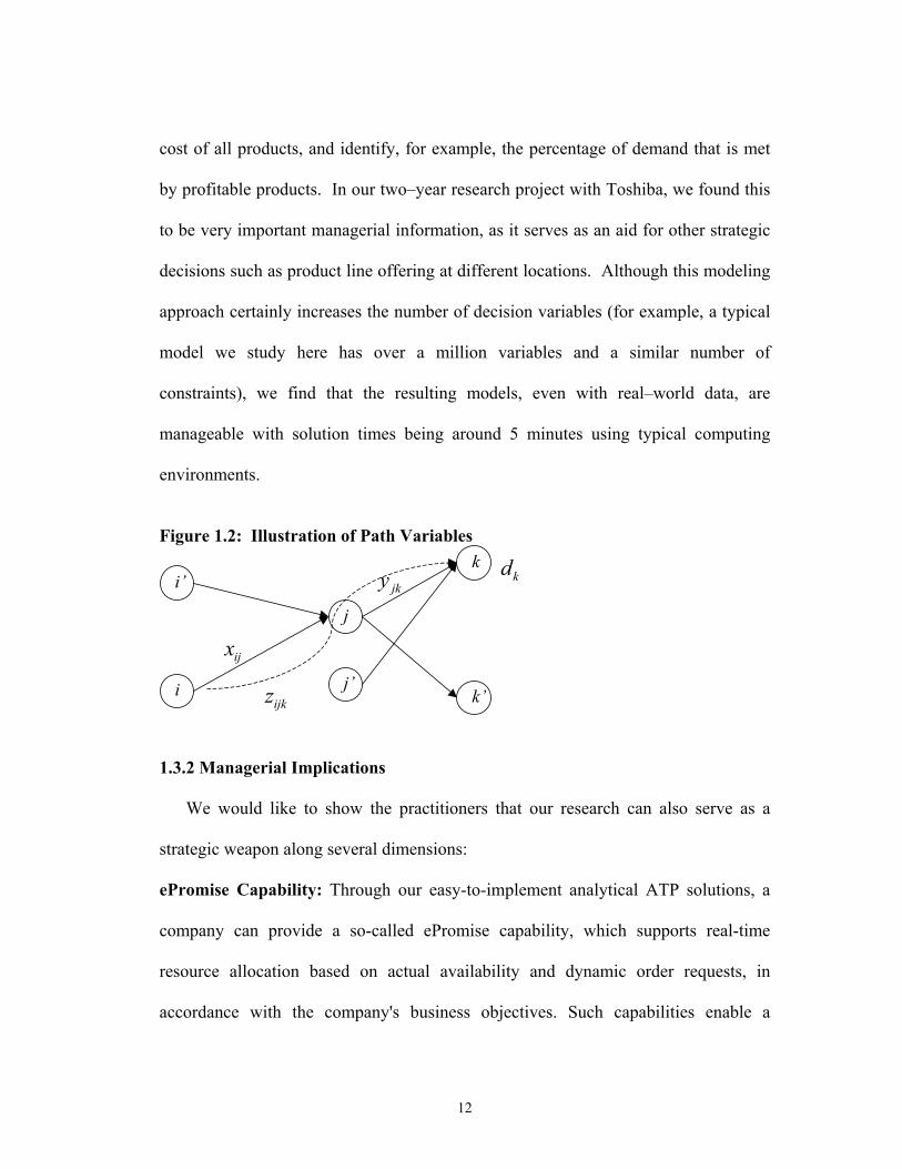
Employing path variables to directly identify and manipulate profitable and
non-profitable products: Unlike most models in the global supply chain literature,
which define variables in terms of flows along a single arc in the network and use
flow balancing constraints at nodes, we employ path variables, which provide
location–specific cost information and directly identify profitable and non–profitable
products (see Figure 1.2). In Figure 1.2, ijx and jky are traditional flow variables for
the product in the network. Demand is represented by kd at node k. Note that this
choice of variables does not capture the unit costs for products sold at node k (for
example, it is not possible to determine whether a particular product at node k comes
from node i or i’.) By defining a path variable ijkz , one can directly determine the unit
12
cost of all products, and identify, for example, the percentage of demand that is met
by profitable products. In our two–year research project with Toshiba, we found this
to be very important managerial information, as it serves as an aid for other strategic
decisions such as product line offering at different locations. Although this modeling
approach certainly increases the number of decision variables (for example, a typical
model we study here has over a million variables and a similar number of
constraints), we find that the resulting models, even with real–world data, are
manageable with solution times being around 5 minutes using typical computing
environments.
Figure 1.2: Illustration of Path Variables
i j’k’
k
j
kd
ijx
jkyi’
ijkz
1.3.2 Managerial Implications We would like to show the practitioners that our research can also serve as a
strategic weapon along several dimensions:
ePromise Capability: Through our easy-to-implement analytical ATP solutions, a
company can provide a so-called ePromise capability, which supports real-time
resource allocation based on actual availability and dynamic order requests, in
accordance with the company's business objectives. Such capabilities enable a

13
company to automate order-promising decisions based on electronic information,
which is essential for an e-commerce environment.
Enhanced Revenue and Service: Embedding the pseudo (future) order into
confirmed orders to deal with uncertainty and finding the “right supplier” to serve the
customer based on varying production status allow companies to identify customers’
real demand and provide a clear understanding of their internal capabilities, thus
enabling managers to enhance service and profit simultaneously.
Buy Smart – How to Benefit from Recession: Our model also identifies the best
quantity of the raw materials/components to buy from suppliers when they offer price
discounts. This helps understand how to coordinate raw material discounts with the
end sales discounts to achieve the best resource utilization. Such a proactive approach
to managing procurement can make a substantial difference during a recession, and
can help managers capitalize on future opportunities. As a result, the proactive
purchaser is able to take advantage of the recession and shape the supply chain to
their long-term advantage.
1.4 Overview of Chapters The remaining chapters in this dissertation are organized as follows. Chapter 2
gives the literature review. In Chapter 3, we introduce an analytical model that
considers multiple confirmed orders, multiple pseudo orders and production pooling.
This model can evaluate the usefulness of responding to customer enquiries in real
time. In Chapter 4, we create mathematical programming models for two scenarios: a

14
company facing a certain demand curve or uncertain demand. These are strategic
level models that provide insight into what quantity levels to purchase from multiple
suppliers based on several cost factors. We also develop a mixed integer
programming model that addresses how to coordinate raw material discounts offered
by s supplier with end-consumers policies. In Chapter 5, we conclude the dissertation
by summarizing the results and the contributions.

15
Chapter 2 Literature Review 2.1 Current ATP Research Traditional ATP systems are based on the Master Production Schedule, which is
derived from the aggregate production plan, detailed end item forecasts, and existing
inventory and orders (Vollman, 1992). Thus, raw materials and production capacity
constraints are taken into account in the MPS to the extent that they were previously
considered in the firm’s aggregate production plan––an infeasible MPS is only
detected after a more detailed resource planning, later in the planning process. In a
differentiated product portfolio, detailed item forecasts can be highly inaccurate,
unexpected demand events are more frequent, and developing a feasible MPS is more
challenging thus compromising the availability of reliable ATP information. It is not
surprising to find several papers (eB2x 2000 ) , (Fordyce and Sullivan, 1999), (Lee
and Billingtion, 1995), (Robinson and Dilts, 1999), and (Zweben, 1996) that discuss
the need for advanced ATP systems, which provide order promising capabilities
based on current capacity and inventory conditions within the firm’s supply chain.
Interestingly, there are relatively few papers that address quantitative models for
order promising. Taylor (1999) introduces a heuristic that keeps track of traditional
ATP quantities to generate feasible due dates for order promising. Kilger (2000) also
proposes a search heuristic to promise orders, motivated by yield management
algorithms used in the airline industry (see below). Ervolina (2001) presents models
16
developed at IBM for resource allocation in a CTO production environment. Moses
(2002) investigates highly scalable methods for real–time ATP that are applicable to
discrete BTO environments facing dynamic order arrivals, focusing on production
scheduling. At an operational level, Yongjin (2002) discusses the relationship
between the performance of dynamic vehicle routing algorithms and online ordering
in conditions of demand saturation––where demand exceeds service capacity. Chen
and Ball (2001) provide mixed–integer programming (MIP) formulations for order
promising and due–date quoting, taking into account existing inventories for raw
materials, components and finished goods, production capacities, and a flexible bill of
materials (BoM) environment (where customers can select different suppliers for the
same raw material). Their models address a static situation, computing ATP
quantities for orders in a batching interval––a batching interval is the time window
over which customer orders are collected before the ATP function is executed to
schedule their production ––which is an input to their models. These models
maximize profit for a batching interval only, without consideration of future
demands. We propose to address the stochastic and dynamic nature of the problem.
More importantly, we address the ATP decision not just from customer response
space, but also from product processing space that includes the product path analysis
and uncertainty. In the following sections, we are going to review these topics.
2.2 Stochastic ATP - Uncertainty In our analytical stochastic model we analyze how to allocate a resource to
optimally promise customer orders when the future orders are uncertain. The problem
17
of allocating scarce capacity to customer orders to promise for future deliveries can
be viewed from another perspective when customers’ sensitivity to lead times (or
their due dates) is significantly different. In this environment, the firm may design a
menu of price and lead–time combinations to segment the market (F.Chen, 2001).
Once the menu is designed, the firm may use operational policies based on resource
rationing to maximize profit. But ATP models and systems are essentially different
from inventory models and systems. Inventory focused systems with different
demand classes, different margins, and with different stock–rationing policies, for
example Kaplan (1969) and Topkis (1968), have dynamic replenishment. There are n
demand classes, and the penalty for not satisfying demand depends on the demand
class (for example, one demand class pays a higher price, or can be met at a lower
cost, thus having a higher priority for the firm). A significant stream of research
exists on inventory rationing, depending on how assumptions of review period,
demand distribution, and unsatisfied demand are handled (Cattani 2002), (Deshpande
and Donhoue, 2001), and (Ha,1997). These models, however, do not consider
capacity limitations in the replenishment decision, and therefore are fundamentally
different from our dynamic ATP models.
A body of literature closely related to this topic is newsvendor-like problems,
which build inventory model to trade off order placing cost and holding cost. The
work of Agrawal and Seshadri (1999) considers a single-period inventory model in
which a risk-averse retailer faces uncertain customer demand and makes a
purchasing-order-quantity and a selling-price decision with the objective of
maximizing expected utility. They analyze how price affects the distribution of the

18
demand and in turn how the quantity to be committed should be determined. The
paper by Cattani (2000) examines a single-period stochastic inventory problem where
N distinct kinds of demand can be satisfied with a single kind of product. But it
assumes that priority is hierarchical -- all demand for a higher priority product is met
before meeting demand for the next lower priority product. Also, we address the
demand pooling effect from economies of the scale, but in Cattani’s paper (2000) the
author studies pooling effect from negatively correlated demands.
2.3 Coordinating Demand Fulfillment with Supply In order to coordinate demand fulfillment with supply, we build models that
identify profitable paths from different suppliers and to different sales subsidiaries.
We provide both an analytical model and a global supply chain MIP model to
investigate that issue, since they involve interactions among several individual factors
as well as thousands of products and product locations. Of the three levels of planning
in a supply chain––strategic, tactical, and operational (see, e.g., Vidal and
Goetschalckx, 1997) ––our models address primarily tactical decisions, that is,
production and distribution decisions that span a maximum of four months, such as
production and transportation choices that maximize profits, subject to capacity and
other constraints. Thus, our models neither address strategic decisions such as facility
location nor operational decisions such as daily production scheduling at plants.
There are several streams of literature that are relevant to our research: global supply
chains, supply chain coordination mechanisms, inventory models with pricing, and

19
product line offering; we review each stream separately and discuss our study
accordingly.
Past literature addresses issues such as supplier–buyer coordination, for example,
an ordering policy that minimizes supply chain costs for both parties (for a review see
Thomas and Griffin, 1996)). Most of these models, however, are stylized extensions
of the basic EOQ model or the Wagner–Within algorithm, focusing on a single
product under independent and deterministic demand. Closely related is the literature
on supply chain contracts (e.g. Bassok and Anupindi 1997, Urban 2000, Chen and
Krass 2001, Serel, Dada and Moskowitz 2001), where, under uncertain demand for a
single product, the buyer commits to a minimum cumulative procurement quantity
over a long–term planning horizon in exchange for price discounts. Our model
differs from the past literature in various aspects: in the analytical model, we consider
demand curves that vary by sales locations; in the resource analysis of Toshiba global
supply chain, we consider a situation where a firm orders a component periodically
(there are no fixed ordering costs), however, the supplier offers a one–time price
discount.
The literature on inventory and pricing is also relevant and extensive––where the
firm decides, in addition to order quantity, on the price of the product (which
influences demand). For a review of single–period models, readers can see Petruzzi
and Dada (1999), and for multi–period models, see Federgruen and Heching (1999),
Chen, Federgruen and Zheng (2001) and Zhao and Wang (2002). Unlike our work,
again, this stream of research assumes a single product with unlimited capacity.
20
Cohen and Lee (1989) argue that differences between supply–chain planning
within a single country and for a global network include the existence of duties,
tariffs, tax rates across countries, currency exchange rates, multiple transportation
modes, and local content rules, among others. There is a considerable body of
research in strategic production–distribution models for global supply chains, and the
reader could refer to Thomas and Griffin (1996), Vidal and Goetschalckx (1997),
Goetschalckx, Vidal and Dogan (2002) for detailed literature reviews. In addition to
production and distribution decisions, this body of literature addresses the more
strategic problem of network design, which is usually formulated as a mixed–integer
programming (MIP) or a non–linear programming (NLP) model. The global nature
of the problem may require careful modeling of transfer pricing (e.g. Vidal and
Goetschalckx 2001), and exchange rates (e.g. Huchzermeier and Cohen 1996).
Our research is also related to the product line offering question––which products
are profitable and should be offered at each location. The literature on the design of a
product line that maximizes profitability focuses primarily on marketing issues, such
as the interactions of a set of products, given their relative utilities and prices, in the
market place (for a review see Yano and Dobson, 1998). A few papers consider the
manufacturing and/or inventory implications of product line breadth (e.g., Van Ryzin
and Mahajan 1999, Smith and Agrawal 2000, Morgan, Daniels and Kouvelis 2001),
such as variable production cost, holding and setup costs, but these papers do not
consider the complex interactions of sourcing, manufacturing, and distribution in
global, capacitated, supply chains, where the profitability of a product can be
different, depending on its supplier or path in the supply chain and the location where
21
it is sold. Summarily, our analysis bridges the gap between sales’ product profitability
and supplier’s variety.
2.4 Revenue Management Finally, we discuss the revenue management literature, which clearly has strong
relevance to our work. Most revenue management models assume fixed (or “almost
fixed”) resource availability, (e.g., airline seats) and balance resource allocation
among multiple demand classes (e.g., fair segment of price-sensitive customers). A
common way to model the airline booking process is to model it as a sequential
decision problem over a fixed time period, in which one decides whether each request
for a ticket should be accepted or rejected. The classical example is that of customers
traveling for leisure and those traveling on business. The former group typically
books in advance and is more price-sensitive, whereas the latter behaves in the
opposite way. Airline companies attempt to sell as many seats as possible to high-fare
paying customers and at the same time avoid the potential loss resulting from unsold
seats. In most cases, rejecting an early (and lower-fare) request saves the seat for a
later (and higher-fare) booking, but at the same time that creates the risk of flying
with empty seats. On the other hand, accepting early requests raises the percentage of
occupation but creates the risk of rejecting a future high-fare request because of the
constraints on capacity. The airline booking problem was first addressed by
Littlewood in 1972, when he proposed what is now known as the “Littlewood Rule”.
Roughly speaking, the rule — proposed for a two class model — says that low-fare
bookings should be accepted as long as their revenue value exceeds the expected
22
revenue of future full fare bookings. This basic idea was subsequently extended to
multiple classes (Belaboba, 1990). Later, it was shown that, under certain conditions,
it is optimal to accept a request only if its fare level is higher or equal to the
difference between the expected total revenues from the current time to the end when
respectively rejecting and accepting the request. This rule immediately leads to the
question “How to evaluate or approximate the expected total revenue from the current
time until the end of booking?” However, the drawback of solving it as a sequential
decision problem is also clear in that the booking policy is only locally optimized and
it cannot guarantee global optimality.
Glover et al. were perhaps the first to describe a network revenue management
problem in airlines. By assuming that passenger demands are deterministic, they
focus on the network aspects of the model (e.g., using network flow theory) rather
than on the stochastic aspect of customer arrivals. Dror, Trudeau, and Ladany propose
a similar network model, again with deterministic demand. The proposed
improvements allow for cancellations, which often happens in the real booking
process. Booking methods based on linear programming were thoroughly investigated
by Williamson (Williamson 1992). The basic models take stochastic demand into
account only through expected values, thus yielding a deterministic program that can
be easily solved. The major drawback of the approach above is that it ignores any
distributional information about the demand.
Later many other industries also applied these techniques to control their
perishable or even non-perishable assets. Weatherford and Bodily (1992) not only

23
propose the new name, Perishable-Asset Revenue Management (PARM), but also
provide a comprehensive taxonomy and research overview of the field. They identify
fourteen important elements for defining revenue management problems. Although
most of these elements are airline-orientated, many ATP problems share the similar
characteristics: particularly the last three modeling-related elements: bumping
procedure (for handling “overbooking”), asset control mechanism (for resource
reservation), and decision rule (for resource allocation). More recently, McGill and
Van Ryzin (1999) classify over 190 research papers into four groups: 1) forecasting,
2) overbooking research, 3) seat inventory control, and 4) pricing. The papers in the
third group are more relevant to ATP models discussed here. For example,
Weatherford and Bodily (1995) present a generic multiple-class PARM allocation
problem. They first study a simplified two-class problem without diversion. The
problem assumes that there are two demand classes, full-price and discount, share the
fixed available capacity of 0q units and that no full-price customer would pay less
than their willingness to pay (i.e., the full price). The purpose is to determine the
number of units that should be allocated to discount-price customers before the
number of full-price customer is realized. The authors further extended the problem
to allow diversion in the multiple-class setting. Sen and Zhang (1999) worked on a
similar but more complicated problem by treating the initial availability as the
decision variable and model the problem as a newsboy problem with multiple demand
classes. To some degree, our work can be seen as the extension of Littlewood two-
class model under the special business setting. Yet due to the characteristics of ATP,
the holding cost and customer service level, which normally is not in the scope of

24
revenue management, are taken into consideration and plays a critical role in our
model (see Chapter 3.2).
25
Chapter 3 Pseudo Order Consideration in Available to Promise (ATP) 3.1 ATP Framework The fundamental decisions ATP models must address are: 1) which orders to
accept 2) the committed quantity for accepted orders. A sophisticated approach to
carry out ATP functionality, introduced by Chen et al. (Chen et. al., 2002), is to
employ large-scale mixed–integer-programming (MIP) models. Other researchers
have also developed ATP models like allocated ATP (a-ATP) and capacity ATP (c-
ATP) to support ATP decision-making process. This model-based approach for ATP
execution can make effective use of resource flexibility and generate reliable order-
promising results. It is indeed efficient in some complicated business environments to
support resource allocation and rescheduling. However, it usually takes more
execution time to solve these models compared to conventional simple finished-
product level ATP search results.
As described in Chapter 1, real-time response is becoming a requirement based on
customer service. Moreover, large numbers of customer orders with both accurate
information and inaccurate configurations may come simultaneously in the e-business
environment and/or large number of customer service channels. With this in mind,
the MIP-based ATP mechanism may not be suitable because of its heavy
computation. In contrast, analytical ATP models, which are based on simple rules and
principles, can provide effective mechanisms for order promising solutions by trading
26
off multiple business objectives under resource constraints. Another benefit of using
analytical models to solve ATP problems is their capability to tackle uncertainty.
Unconfirmed customer orders can capture real-life customer’s inquiry and order
cancellation, which is difficult for MIP types of models to handle. Undoubtedly, a
further advantage of analytical models is that they offer generic solutions that don’t
require extensive experiments.
In this chapter, an analytical ATP model will be introduced for order-
promising and fulfillment decisions based on consideration of both profit and
customer service. Instead of putting the customer service level in the constraints, we
include it in the objective function. This reflects the trend toward pushing the service
levels as high as possible. Other feature of this analytical ATP model is: A pseudo
order with stochastic characteristics is considered with other confirmed orders to
represent uncertain customer inquires and order cancellations. Since one pseudo order
may have a higher profit margin but also uncertainty, it will have an impact on the
commitment of the confirmed orders. It’s worth mentioning here that the uncertainties
in ATP are mainly caused by three factors: demand, lead-time and raw material
purchasing price. According to Weber’s survey (Weber and Current 2000), the effect
of lead time is only 10-20% of effect of demand on a company’s total profit. On the
other hand, the uncertainty from purchase price can be compromised by supply
contracts as analyzed in our model. Thus we believe that using a pseudo order to
incorporate the current orders and future orders together not only reflects price
uncertainty in rapidly changing environment, but also captures the Achilles’ heel.

27
We shall see that our objective function is neither convex nor concave, but a d.c.
function, i.e. a function that can be represented as the difference of two convex
(concave) functions (Horst, 1993). The problem of maximizing a d.c. function under
linear constraints is a nonconvex global optimization problem, which may have
multiple local minima with substantially different values. Such multiextremal
problems cannot be solved by standard methods of nonlinear programming which can
at best locate a local minimum. Outer approximation methods along with branch and
bound methods for finding a global minimum have been suggested in (Tuy, 1987).
However, most of these methods are able to solve limited size problem instances.
This should not be surprising, since the problem is known to be NP-hard, see e.g.
(Pardalos, 1984). Therefore, simultaneous consideration of the uncertain demand
makes the problem more general, and also more difficult. Fortunately, we have
derived some rule-based solutions which are presented later in this section.
3.2 Problem Formulation & Model The problem under consideration is a single period, single product, multi-order
ATP model. This model consists of N confirmed customer orders, which are assumed
to be deterministic, and one pseudo order, which is stochastic. The fundamental
decision in the model is to determine promised order quantities for the confirmed
customer orders and a reserved quantity for the pseudo order by considering both
production impact and material limitations. The objective of including the pseudo
order is to anticipate near-term future customer orders based on customer inquiry

28
information. The resultant model is a constrained non-linear stochastic programming
problem.
In the model, we use “total benefit” as the objective function, which is defined as
the sum of weighted expected profit and customer service level. This reflects
common practice in most order fulfillment and optimization processes. The relative
weights of expected profit and customer service level can be adjusted in the model to
reflect their importance in specific business settings. Meanwhile, we assume the
committed quantity of the confirmed order can never exceed the requested quantity.
For the stochastic pseudo order, holding costs may be incurred if the committed
quantity is greater than the specified quantity. Below is the notation that will be used
in the formulation.
3.2.1 Notation and Remarks on Function Properties Let { }NI ,,2,1 L= be the index of a set of the confirmed customer orders. For all
Ii ∈ , let iq and ir be the requested quantity and sales price of the confirmed order i ,
respectively; iβ is a weighted constant of the customer service level for the
confirmed order i . For the pseudo order, let u be the pseudo order quantity, which is
a random variable with known probability density function (PDF) as )(⋅f , and p , h
the unit sales price and unit holding cost, respectively.
For the order promising decision, we consider two kinds of resources: material
availability and production capacity. Here, we assume the production cost is a convex
function of the quantity produced. A convex production cost exhibits non-increasing
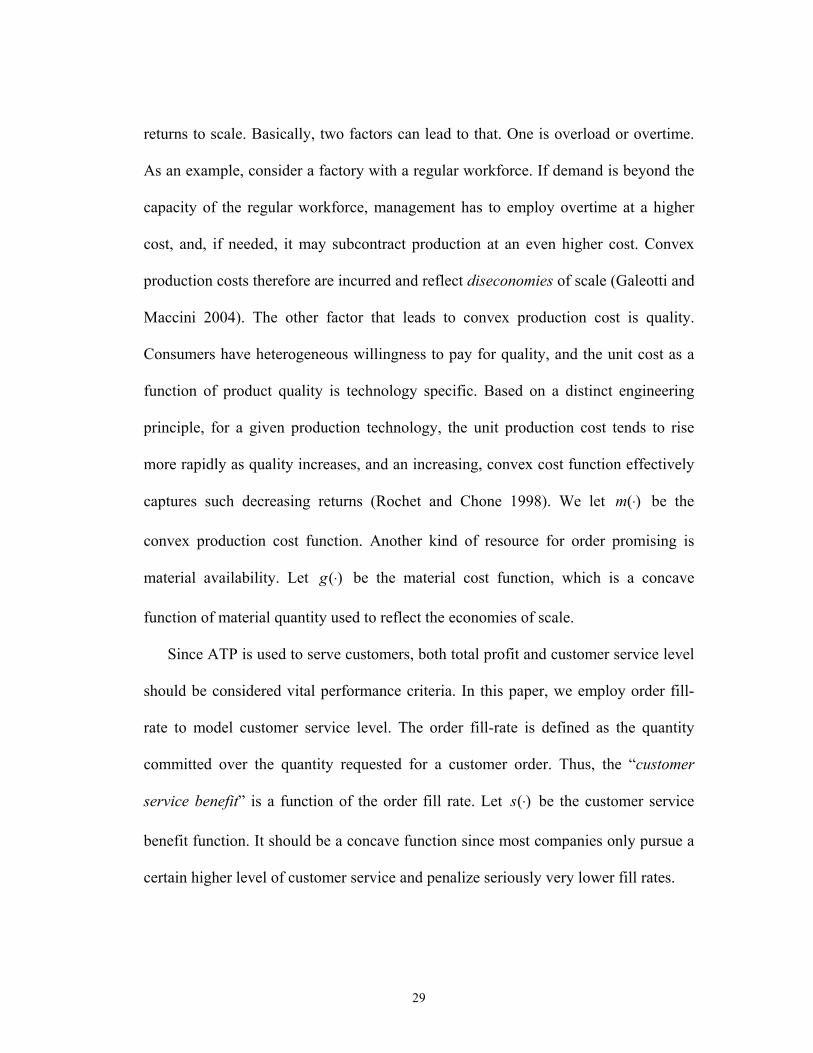
29
returns to scale. Basically, two factors can lead to that. One is overload or overtime.
As an example, consider a factory with a regular workforce. If demand is beyond the
capacity of the regular workforce, management has to employ overtime at a higher
cost, and, if needed, it may subcontract production at an even higher cost. Convex
production costs therefore are incurred and reflect diseconomies of scale (Galeotti and
Maccini 2004). The other factor that leads to convex production cost is quality.
Consumers have heterogeneous willingness to pay for quality, and the unit cost as a
function of product quality is technology specific. Based on a distinct engineering
principle, for a given production technology, the unit production cost tends to rise
more rapidly as quality increases, and an increasing, convex cost function effectively
captures such decreasing returns (Rochet and Chone 1998). We let )(⋅m be the
convex production cost function. Another kind of resource for order promising is
material availability. Let )(⋅g be the material cost function, which is a concave
function of material quantity used to reflect the economies of scale.
Since ATP is used to serve customers, both total profit and customer service level
should be considered vital performance criteria. In this paper, we employ order fill-
rate to model customer service level. The order fill-rate is defined as the quantity
committed over the quantity requested for a customer order. Thus, the “customer
service benefit” is a function of the order fill rate. Let )(⋅s be the customer service
benefit function. It should be a concave function since most companies only pursue a
certain higher level of customer service and penalize seriously very lower fill rates.

30
To formulate the committed quantity of the customer orders, we define the
following decision variables. For all Ii ∈ , let:
iX equals the committed quantity of the confirmed order i ;
Y equals the committed quantity of the pseudo order.
3.2.2 Model Formulation Based on the previous notation, the total revenue, which comes from both
confirmed customer orders and the pseudo order, can be formulated as
∑∈
+Ii
ii uYpMinXr ),()( , (3.1)
Where the first term is the confirmed order’s revenue, and the second term is the
pseudo order’s revenue. We assume that the production cost and material cost are
both measured in terms of a unit of product. Then, the material used is proportioned
to the number of products committed to customers. The material cost and production
cost is given as equation (3.2) and (3.3), respectively.
)(∑∈
+Ii
i YXg (3.2)
)(∑∈
+Ii
i YXm (3.3)
The holding cost incurred by the pseudo order will be:
)0,( uYMaxh −× . (3.4)
Hence, the total expected profit is:
EP = ),(( uYpMinEXrIi
ii +∑∈
- )( YXgIi
i +∑∈
- )( YXmIi
i +∑∈
- ))0,(( uYMaxEh −× (3.5)
31
Substituting the expected revenue and holding cost of the pseudo order into the PDF
function in the above equation yields:
EP = )())()((0
YXgduufYduuufpXrIi
iY
Y
Iiii +−++ ∑∫∫∑
∈
∞
∈
∫∑ −−+−∈
Y
Iii duufuYhYXm
0
)()()( (3.6)
We note that the unit profit margin of an individual customer order may be
negative like most discount sales. The reason to promise such orders is due to
customer service level considerations. For the ith customer order, the customer
service level, specifically, order fill rate, is ii qX . Hence, the total customer service
benefit from all customer orders can be represented as below:
∑∈Ii i
ii q
Xs )(β (3.7)
in which iβ is the customer service benefit weight. The value of iβ indicates the
importance of customer service in comparison to profit for the ith customer order.
Therefore, the objective function, which is defined as the “benefit function” since it
includes both profit and customer service level, can be written as:
TB = )())()((0
YXgduufYduuufpXrIi
iY
Y
Iiii +−++ ∑∫∫∑
∈
∞
∈
)()()()(0
∑∫∑∈∈
+−−+−Ii
qX
i
Y
Iii i
isduufuYhYXm β (3.8)
subject to constraints described as following:
0≥− ii Xq (3.9)
32
0≥iX (3.10)
0≥Y (3.11)
Constraints (3.9), (3.10) and (3.11) are order-promising limitations and non-
negativity. They are similar to the widely accepted concept of “booking limits” or
“protection level” in the revenue management area.
Using the Lagrange method, the first order condition of the problem (3.8)-(3.11) can
be given as follows for all Ii ∈ .
0)()(')(' =+−′++−+− ∑∑∈∈
iiqX
qIi
iIi
ii i
i
i
i sYXmYXgr μλβ (3.12)
0)()(')('))(1( =+−+−+−− ∑∑∈∈
wYhFYXmYXgYFpIi
iIi
i (3.13)
0)( =− iii Xqλ (3.14)
0=× iXμ (3.15)
0≥iλ (3.16)
0≥iμ (3.17)
0=×Yw (3.18)
0≥w (3.19)
Where iλ , iμ and w are Lagrange multipliers for constraints (3.9), (3.10) and (3.11),
respectively.
3.2.3 Model Analysis

33
As stated earlier the objective function is neither convex nor concave, but a d.c.
function. We present the following Theorem to assure the existence of optimal
solution for the problem (3.8)-(3.11). The proof is shown in Appendix 1.
Theorem 3.1: The objective function defined by (3.8) will be strictly concave on the
feasible region defined by problem (3.9)-(3.11) if,
1))(,(
++−>
nKphLUMaxM (3.20)
Where )(''10
xsMaxUx≤≤
= ; 21i
i
ni qMinL
β≤≤
= ; )(00
yfMinKyy≤≤
= with )(10 hp
pFy+
= − ; and
)]('')(''[00
zmzgMinMzz
+=≤≤
with ∑=
+=n
iiqyz
100 .
Remark 3.1: There exists one and only one optimal solution for the nonlinear
stochastic problem (3.8)-(3.11) if )(⋅g is a concave function, )(⋅s is a strictly concave
function, and
0)('')(" >⋅+⋅ mg (3.21)
Proof: see Appendix 2.
One can observe that condition (3.21) is the special case of condition (3.20).
Theorem 3.1 gives conditions for the existence of an optimal solution for the problem
(3.8)–(3.11). Condition (3.20) basically states that the total cost (production cost plus
material cost) function should be “convex enough” to compensate the concaveness of
projected customer service level functions.

34
Obviously, the problem (3.8)–(3.11) is a multiple constrained newsvendor
problem, which has been shown by Lau (1995) to be very difficult to solve, and not
much work has been done on capacitated systems (Tayur, 1998). From an order
promising point of view, we are more interested in the solution structure, rather than
the solution itself, of the problem since the solution structure can provide insights and
guidance for optimal order promising. We present the following Theorem to illustrate
the structure of the solutions for the problem (3.8)-(3.11).
Theorem 3.2: For ,, Iji ∈∀ if the following condition holds
0)]1(')][0('[ ≥−− sZsZ ijij , (3.22)
where ijZ is defined by Equation (3.23) with j
j
i
iij qq
ββα −=
⎪⎩
⎪⎨⎧
−=−
= Otherwise ,
0 ,1
ij
ji
ij
ijrr
ifZ
α
α (3.23)
then there exist two points Ikk ∈′, )'( kk ≤ , the optimal solutions of problem (3.8)-
(3.11) have the following structure:
0=iX for all 'ki < ,
ii qX = for all ki > ,
*iX for all kik ≤≤′ is solved from the following equations:
])(')('[)('11
*
i
n
ll
n
ll
i
i
k
i rYXmYXgqqXs −+++= ∑∑
==β (3.24)

35
hp
YXmYXgpYF
n
ii
n
ii
+
+−+−=
∑∑==
)(')(')( 11 (3.25)
Proof: see Appendix 3.
Theorem 3.2 provides the structure of the optimal solution. Based on this
Theorem we can see that some customer orders should be one hundred percent
committed, and some others should not committed at all when the conditions above
are hold. The ijZ variable can be interpreted as the ratio between profit and customer
service level, and Theorem 3.2 just states how a particular customer order promising
scheme should be adopted depending on that ratio.
Remark 3.2: If the following condition holds, ,Ii ∈∀
11
1 )1(')0(' ++
+ +<+ ii
ii
i
i rsq
rsq
ββ, (3.26)
then the optimal solution for problem (3.8)–(3.11) is as given in Theorem 3.2 with
kk ′= .
Proof: see Appendix 4.
From this remark, one can observe that the optimal order commitment policy is
characterized by a single key order, which represents a threshold between orders
whose quantities are either 0 or iq . That quantity can be found by simply searching
the linear solution space I. This gives us a simplified policy to make the optimal
order promising for customers.

36
In real life situations, one company may only concentrate on a single criteria,
choosing between customer service level and profit in order promising practices. In
such case, condition (3.22)-(3.23) in Theorem 3.2 can be further simplified as the
following:
In the case when product sales price plays a dominant role in order promising
practice, condition (3.22)-(3.23) becomes (3.27) in deriving optimal solution
to problem (3.8)-(3.11) in Theorem 3.2.
,1 lcrr ii >−+ where )()0('
i
iqMaxsc β= Il ∈ (3.27)
This solution structure can be easily checked and allows sales personnel to
determine how the orders should be committed. When 1=l , then there exists
one and only one solution.
In the case when customer service level plays a dominant role in order
promising practice, condition (3.22)-(3.23) would be simplified to (3.28) in
Theorem 3.2.
1
1
+
+<i
il
i
i
qqβεβ
where )1(')0('
ss=ε (3.28)
This is symmetric to condition (3.27).
Remark: Extension of Littlewood Model
We can also explain the work above from the perspective of revenue
management. If we aggregate all the confirmed orders into one class (since they are
all deterministic and order promising can be easily carried out by ordering the price
37
from high to low), and the problem represented by (3.8-3.11) becomes tradeoff of
pseudo order class and confirmed order class. This is a two-class revenue
management problem except we take customer service level into consideration. Thus,
it can be viewed as an extension of the Littlewood two-class model under a special
business setting. For example, if we manipulate this equation and treat Y as the
optimal booking of (3.25)
hp
YXmYXgpYF
n
ii
n
ii
+
+−+−=
∑∑==
)(')(')( 11
Then we have
hp
YXmYXghYF
n
ii
n
ii
+
++++−=
∑∑==
)(')('1)( 11
1
21)(ppYF −= (the Littlewood two-class model )
where )(')('11
2 YXmYXghpn
ii
n
ii ++++= ∑∑
==
and hpp +=1
This result is in the form of Littlewood model. Belobaba (1987a) heuristically
extends Littlewood’s rule to multiple fare classes and introduces the term Extended
Marginal Seat Revenue (EMSR) for the general approach. The EMSR method does
not produce optimal booking limits except in the two-fare case, and Robinson (1995)
shows that, for more general demand distributions, the EMSR method can produce
arbitrarily poor results. There has been very little published research on joint capacity
allocation/pricing decisions in the revenue management context. Weatherford (1994)

38
presents a formulation of the simultaneous pricing/allocation decision that assumes
normally distributed demands, and models mean demand as a linear function of price.
The corresponding expressions for total revenue as a function of both price and
allocation are extremely complex, but no structural results are obtained. However, our
study not only obtains the structural results but also shows the impact of holding costs
on both pseudo order and confirmed order quantities.
More importantly, our model takes service level into consideration and allows not
only 100% or 0% commitment but also portion commitment for each single order,
unlike most discussions in the field of Airline or Yield Management. Formulas (3.26)
(3.27) and (3.28) describe the rule of the accepting or rejecting order, which is
determined by different order parameters such as price and SL. We can see the
order’s “marginal benefit”, characterized in Remark 3.2, includes both price and SL;
the “marginal revenue” as defined in the Littlewood rule and extended EMSR
(Expected Marginal Seat Revenue) model in other Revenue Management research,
includes only one parameter (price). ). Thus, our work can be viewed as extending
prior revenue management research.
3.3 Implementation Rule
The analysis above provides decision makers the effective rule-based mechanism
to implement and deploy critical decisions in real-time ATP systems. We summarize
and illustrate it in Figure 3.1.

39
3.4 Experimental Study and Results Our goal in developing analytical ATP model is to develop real-time strategies to
support order-promising process. In order to gain strategic insight from the model
numerically, we design and carry out the following experiments.
Figure 3.1 Pseudo order decision flow chart
Material economies of Scale.
Company Level
Theorem 3.1 or g’’(.)+m’’(.) >0
No Yes
Yes
Condition (3.22)
Order Level
Yes
Optimal Solution Structure
Customized Goal

40
The cost and service level functions are assumed to be as following:
ατ )()( += iiii qXqXs )10( << α
γ)()( 1 YXkYXmIi
iIi
i +=+ ∑∑∈∈
)10( << γ
λ)())(( 2 YXkYXgIi
iIi
i +=+ ∑∑∈∈
)1( >λ
),()( δμNYf =
where the coefficients are given as below:
800=iβ 3=h
9.0=α 1=l ,
431 =k 8.0=γ
002.02 =k 2=λ
Four confirmed orders and one pseudo order are considered in this experiment with
specifications as below:
51 =r 82 =r 123 =r 184 =r 20=p
4004321 ==== qqqq , 500=μ , 70=δ
By using MathCAD software, we have the solution:
=),,,,( 4321 YXXXX (0, 0, 383.5, 400, 619.2)
We can observe that the solution has the exact same structure as Theorem 3.2 states.
Now let’s see some interesting findings from the experiments.
1) The pseudo order’s price sensitivity analysis:

41
Table 3.1: Effect of Pseudo Order’s Price Change
Y's Price X1 X2 X3 X4 Y SUM(X) TB
18 0 0 387.2 400 614 787.2 6391
19 0 0 385.8 400 617 785.8 6860
20 0 0 383.5 400 619 783.5 7330
21 0 0 381 400 621 781 7802
22 0 0 380 400 623 780 8276
Figure 3.2 Committed Order as a function of pseudo order’s Price
Y's Price vs. SUM(X),Y
600
650
700
750
800
18 19 20 21 22Y's Price
SUM
(X),
Y
SUM(X) Y
42
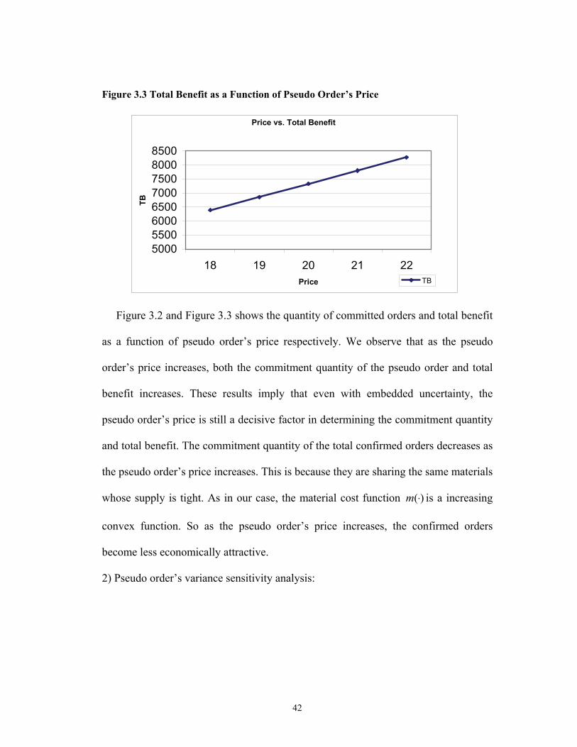
Figure 3.3 Total Benefit as a Function of Pseudo Order’s Price
Price vs. Total Benefit
50005500600065007000750080008500
18 19 20 21 22Price
TB
TB
Figure 3.2 and Figure 3.3 shows the quantity of committed orders and total benefit
as a function of pseudo order’s price respectively. We observe that as the pseudo
order’s price increases, both the commitment quantity of the pseudo order and total
benefit increases. These results imply that even with embedded uncertainty, the
pseudo order’s price is still a decisive factor in determining the commitment quantity
and total benefit. The commitment quantity of the total confirmed orders decreases as
the pseudo order’s price increases. This is because they are sharing the same materials
whose supply is tight. As in our case, the material cost function )(⋅m is a increasing
convex function. So as the pseudo order’s price increases, the confirmed orders
become less economically attractive.
2) Pseudo order’s variance sensitivity analysis:

43
Table 3.2 Effect of Pseudo Order’s Variance
Variance
of Y X1 X2 X3 X4 Y SUM(X) TB
60 0 0 394.5 400 606.7 794.5 7639
70 0 0 383.5 400 619.2 783.5 7330
80 0 0 373 400 630 773 7031
90 0 0 360.6 400 641.5 760.6 6741
100 0 0 352.5 400 651.5 752.5 6458
Figure 3.4 Committed Order Quantity as a Function of Pseudo Order’s Variance
Y's Variance
550
600
650
700
750
800
850
60 70 80 90 100
SUM
(X),
Y
SUM(X) Y

44
Figure 3.5 Total Benefit as a Function of Pseudo Order’s Variance
Variance vs. Total Benefit
6000
6500
7000
7500
8000
60 70 80 90 100Variance
TB
TB
Figure 3.4 shows the committed order quantity as a function of the pseudo order’s
variance. As variance increases, the total commitment quantity of confirmed order
decreases, and the commitment quantity of the pseudo order increases. Note that the
reason that more pseudo orders are committed is to offset the larger uncertainty, not
to generate more profit, as evidenced by Figure 3.5, the total benefit decreases when
variance and commitment quantity of the pseudo order increase. This is an interesting
finding and reveals that uncertainty of the forecasted order will not only lead to the
bullwhip effect via information distortion, but ultimately will hurt the efficiency of
the supply chain in the form of excess raw material inventory, misguided production
schedules, missed target orders, and poor customer service levels. Predictably, more
and more companies are adopting the various cutting-edge technologies like
Electronic Data Interchange (EDI) to improve their forecasting ability and mitigate
such uncertainty.
3) The service level sensitivity analysis:
45
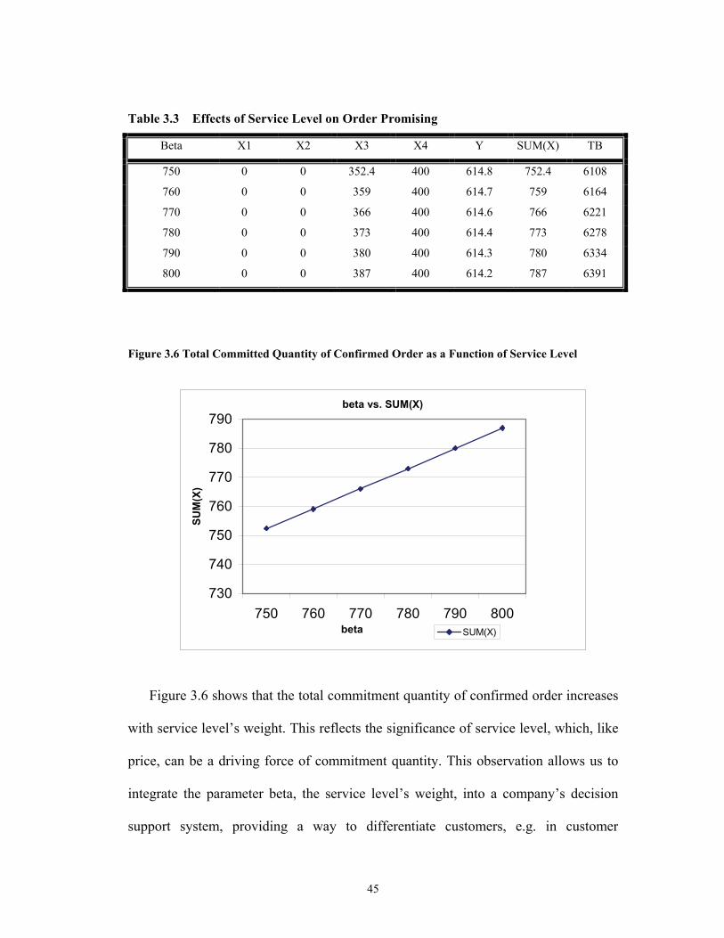
Table 3.3 Effects of Service Level on Order Promising
Beta X1 X2 X3 X4 Y SUM(X) TB
750 0 0 352.4 400 614.8 752.4 6108
760 0 0 359 400 614.7 759 6164
770 0 0 366 400 614.6 766 6221
780 0 0 373 400 614.4 773 6278
790 0 0 380 400 614.3 780 6334
800 0 0 387 400 614.2 787 6391
Figure 3.6 Total Committed Quantity of Confirmed Order as a Function of Service Level
Figure 3.6 shows that the total commitment quantity of confirmed order increases
with service level’s weight. This reflects the significance of service level, which, like
price, can be a driving force of commitment quantity. This observation allows us to
integrate the parameter beta, the service level’s weight, into a company’s decision
support system, providing a way to differentiate customers, e.g. in customer
beta vs. SUM(X)
730
740
750
760
770
780
790
750 760 770 780 790 800beta
SUM
(X)
SUM(X)

46
relationship management (CRM) system. This provides an approach to offer superb
service levels to the most valuable customers, develop strategies for unprofitable
customers, and differentiate proactively the handling of different needs-based
customer categories. Simply put, look for individual solutions rather than mass
solutions.
3.5 Multiple Pseudo Orders in ATP
We further consider the case that captures more facts in real-life: a company not
only has multiple confirmed orders, but also has multiple pseudo orders to fulfill. The
stochastic characteristics associated with pseudo orders represent uncertain customer
inquires and order cancellations. Particularly, we are interested to see what
commitment decisions should be made if those pseudo orders’ profit function is
concave of the order quantity. This is very true in most of the mass-production
environments such as lot-by-lot manufacturing process, or pallet-by-pallet
transportation among semi-final and final assembly factories.
3.5.1 Notation
The problem under consideration is a single period, single product, multi-order
ATP model. The model consists of N confirmed customer orders, which are assumed
to be deterministic; and M pseudo orders, which are stochastic. The fundamental
decision in the model is to determine promised order quantities for the confirmed
customer orders and the reserved quantity for the pseudo orders by considering both

47
production impact and material limitations. The objective of including the pseudo
order is to anticipate near-term future customer orders based on customer inquiry
information. The resultant model is a constrained non-linear stochastic programming
problem.
In the model, we use “total benefit” as the objective function, which is defined as
the sum of weighted expected profit and customer service level. This reflects
common practice in most order fulfillment and optimization processes. The relative
weights of expected profit and customer service level can be adjusted in the model to
reflect their importance in specific business settings. Meanwhile, we assume the
committed quantity of the confirmed order can never exceed the requested quantity.
For the stochastic pseudo orders, holding costs may be incurred if the committed
quantities are greater than the specified quantity.
Let { }NI ,,2,1 L= be the index of a set of the confirmed customer orders. For all
Ii ∈ , let iq and ir be the requested quantity and sales price of the confirmed order i ,
respectively; iβ a weighted constant of the customer service level for the confirmed
order i . Let { }MJ ,,2,1 L= be the index of a set of the pseudo orders, jp and jh the
unit sales price and unit holding cost of the pseudo order j, respectively. u is the
pseudo order quantity, which is a random variable with known probability density
function (PDF) as )(⋅f .
As described in section 3.2.1, let )(⋅g be the concave material cost function and
)(⋅m be the convex production cost function. Also, let )(⋅s be the customer service
benefit function. We model this function as a concave function, which would reflect a
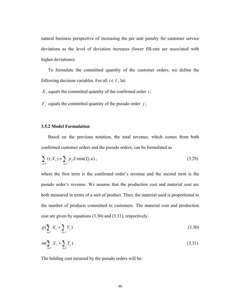
48
natural business perspective of increasing the per unit penalty for customer service
deviations as the level of deviation increases (lower fill-rate are associated with
higher deviations).
To formulate the committed quantity of the customer orders, we define the
following decision variables. For all Ii ∈ , let:
iX equals the committed quantity of the confirmed order i ;
jY equals the committed quantity of the pseudo order j ;
3.5.2 Model Formulation
Based on the previous notation, the total revenue, which comes from both
confirmed customer orders and the pseudo orders, can be formulated as
∑ ∑∈ ∈
+Ii Jj
jii uYjEpXr ),min()( , (3.29)
where the first term is the confirmed order’s revenue and the second term is the
pseudo order’s revenue. We assume that the production cost and material cost are
both measured in terms of a unit of product. Then, the material used is proportional to
the number of products committed to customers. The material cost and production
cost are given by equations (3.30) and (3.31), respectively.
)(∑ ∑∈ ∈
+Ii Jj
ji YXg (3.30)
)(∑ ∑∈ ∈
+Ii Jj
ji YXm (3.31)
The holding cost incurred by the pseudo orders will be:

49
∑∈
−Jj
jj uYEh )0,max( . (3.32)
Hence, the total expected profit is:
)(),min( ∑∑∑∑∈∈∈∈
+−+=Jj
jIi
iJj
jjIi
ii YXguYEpXrTP
)0,max()( ∑∑∑∈∈∈
−−+−Jj
jjJj
jIi
i uYEhYXm (3.33)
We note that the unit profit margin of an individual customer order could be negative
like most discount sales. The reason to promise such orders is due to customer service
level considerations. For the ith customer order, the customer service level,
specifically, order fill rate, is qX i . Hence, the total customer service benefit from all
customer orders can be represented as below:
∑∈Ii i
ii q
Xs )(β (3.34)
in which iβ is the customer service benefit weight. The value of iβ indicates the
importance of customer service in comparison to profit for the ith customer order.
Therefore, the objective function, which is defined as the “reward function” since
it includes both profit and customer service level, can be written as:
TB = )(),min( ∑∑∑∑∈∈∈∈
+−+Jj
jIi
iJj
jjIi
ii YXguYEpXr
)()0,max()( ∑∑∑∑∈∈∈∈
+−−+−Ii
qX
iJj
jjJj
jIi
i i
isuYEhYXm β (3.35)
subject to constraints described as following:
0≥− ii Xq (3.36)
0≥iX (3.37)

50
0≥jY (3.38)
Constraints (3.36), (3.37) and (3.38) are order-promising limitations and non-
negativity.
Using the Lagrange method, the first order condition of the problem (3.35)-(3.38) can
be given as follows for all Ii ∈ .
0)()(')(' =+−′++−+− ∑∑∑∑∈∈∈∈
iiqX
qJj
jIi
iJj
jIi
ii i
i
i
i sYXmYXgr μλβ (3.39)
0)()(')('))(1( =+−+−+−− ∑∑∑∑∈∈∈∈
jjjJj
jIi
iJj
jIi
ijj wYFhYXmYXgYFp (3.40)
0)( =− iii Xqλ (3.41)
0=× iXμ (3.42)
0≥iλ (3.43)
0≥iμ (3.44)
0=× jj Yw (3.45)
0≥jw (3.46)
Where iλ , iμ and w are Lagrange multipliers for constraints (3.36), (3.37) and (3.38),
respectively.
3.5.3 Model Analysis
Lemma 3.5.1 : The profit function of pseudo orders is concave in terms of order
quantity.
Proof: See Appendix 5.
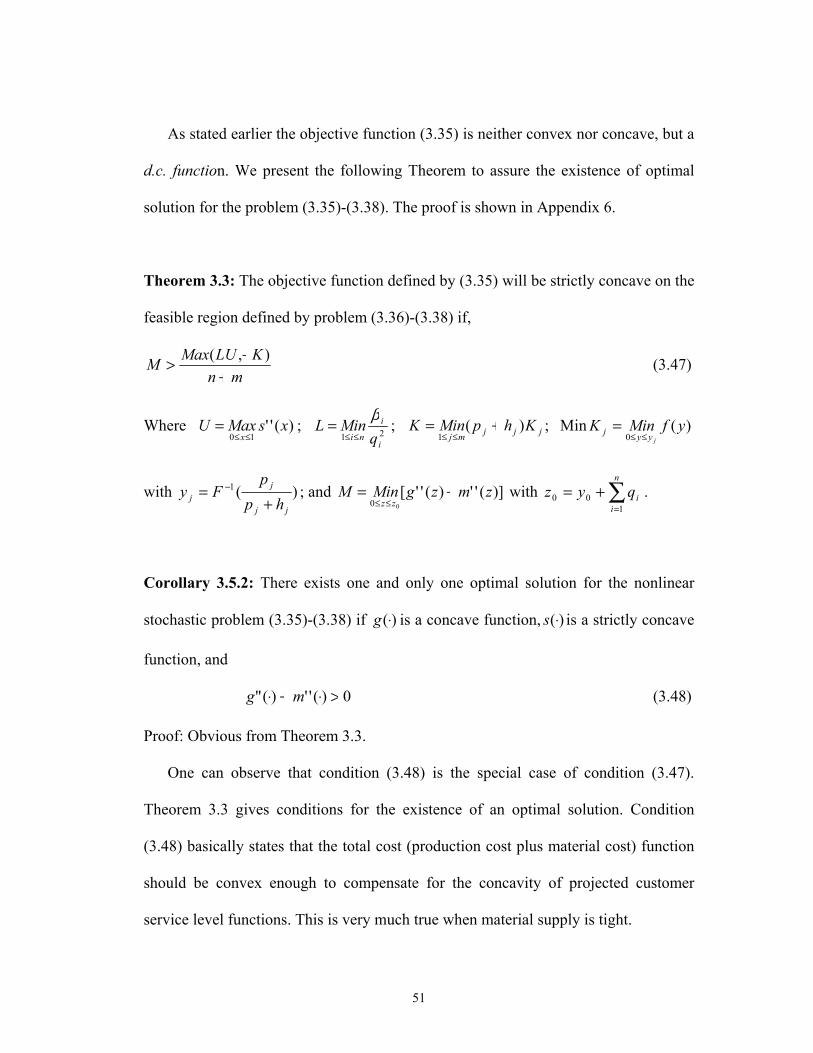
51
As stated earlier the objective function (3.35) is neither convex nor concave, but a
d.c. function. We present the following Theorem to assure the existence of optimal
solution for the problem (3.35)-(3.38). The proof is shown in Appendix 6.
Theorem 3.3: The objective function defined by (3.35) will be strictly concave on the
feasible region defined by problem (3.36)-(3.38) if,
mnKLUMaxM
+−> ),( (3.47)
Where )(''10
xsMaxUx≤≤
= ; 21i
i
ni qMinL
β≤≤
= ; jjjmjKhpMinK )(
1+=
≤≤; Min )(
0yfMinK
jyyj ≤≤=
with )(1
jj
jj hp
pFy
+= − ; and )]('')(''[
00zmzgMinM
zz+=
≤≤ with ∑
=+=
n
iiqyz
100 .
Corollary 3.5.2: There exists one and only one optimal solution for the nonlinear
stochastic problem (3.35)-(3.38) if )(⋅g is a concave function, )(⋅s is a strictly concave
function, and
0)('')(" >⋅+⋅ mg (3.48)
Proof: Obvious from Theorem 3.3.
One can observe that condition (3.48) is the special case of condition (3.47).
Theorem 3.3 gives conditions for the existence of an optimal solution. Condition
(3.48) basically states that the total cost (production cost plus material cost) function
should be convex enough to compensate for the concavity of projected customer
service level functions. This is very much true when material supply is tight.

52
From an order promising point of view, we are more interested in the solution
structure rather than the solution itself, since the solution structure can provide
insights and guidance for optimal order promising. We present the following
Theorem to illustrate the structure of the solutions for the problem (3.35)-(3.38).
Theorem 3.4:
For confirmed orders, we have:
Let jiij rrZ −= and j
j
i
iij qq
ββα −= . If we assume, ,, Iji ∈∀
0)]1(')][0('[ ≥++ sZsZ ijijijij αα .
Then there exist two points Ikk ∈′, )k'k( ≤ such that the optimal solution
, ;
' ;' ;0
*
⎪⎩
⎪⎨
⎧
>∀≤≤∀
<∀
=kiq
kikXki
X
i
ii Where *iX solves equation
])(')('[)('111 1
*
i
m
jj
n
ll
n
l
m
jjl
i
i
k
i rYXmYXgqqXs −+++= ∑∑∑ ∑
=== =β (3.49)
For pseudo orders: we have:
If we assume mppp ≤≤≤ L21 , then there exists Ik ∈′′ such that
⎪⎩
⎪⎨⎧
′′≥∀
′′<∀=
kjYkj
Yj
j ; ;0
* , where *jY solves equation

53
jj
m
ll
n
ii
m
ll
n
iij
j hp
YXmYXgpYF
+
+−+−=
∑∑∑∑====
)(')(')( 1111* (3.50)
Proof: see Appendix 7.
Theorem 3.4 provides a simple structure for the optimal solution for both
confirmed orders and pseudo orders: some customer orders should be one hundred
percent committed, and some others should not be committed at all. More
specifically, confirmed orders’ commitment quantities are determined by K and K’
and pseudo orders’ commitment quantities are determined by K. Therefore we only
need to compute K, K’ for confirmed orders and K” for pseudo orders.
The interpretation for ijZ and iβ are the ratio between profit and customer service
level, and Theorem 3.4 just states how a particular customer order promising scheme
should be adopted depending on that ratio.
Corollary 3.5.3: For ,Ii ∈∀ if the following condition holds,
11
1 )1(')0(' ++
+ +<+ ii
ii
i
i rsq
rsq
ββ, (3.51)
then the optimal solution for problem (3.35)–(3.38) would be as given in Theorem 3.4
with kk ′= . Moreover, we have }),()(|min{arg ** Jjqmqgpjk j ∈′+′>≥′′ , where
∑+=
=n
kiiqq
1
* .

54
Proof: see Appendix 8.
From this Corollary, one can observe that the optimal order commitment policy is
decided by only one order commitment, and the others becomes either 0 or iq if the
condition (3.51) is satisfied. That quantity can be found by simply searching the
linear solution space I+J. It gives us a simplified policy to make the optimal order
promising for customers.
3.6 Remarks It is clear to see that demand uncertainty will not only lead to the bullwhip effect
via information distortion, but ultimately will hurt the efficiency of a supply chain in
the form of excess raw material inventory, misguided production schedules, missed
target orders, and poor customer service level. Our analytical ATP model, as the core
of customer-driven order management, indeed provides the manager with useful
insights to conquer the resulting problems. Our models can provide guidance in both
customer-service dominant and profit dominant business environments.
There are two other types of approaches to pseudo orders promising: a traditional
simulation-based approach and the more recent “scenario generation” approach. The
simulation-based approach for promising the delivery of future orders is based on
dynamic buffer adjustment coupled with forecasting the amount of buffer required.
The primary objective of that is to frame the problem and suggest methods of
analysis. Since this approach is simulation-based, optimal policies or solutions are

55
not obtained; simulation run times can also grow very large, e.g. from tens of
minutes to several days to run one data set. Grant and Moses (2002) applied this
approach but have to deal with an issue that inherently exists in this methodology:
multiple yet conflicting performance measures, such as average lateness to promise,
variance of the lateness to promise, and constraining the probability of a failed
promise. We can see, all of these ask for more rather than less judgment calls from
decision-makers. We should also note that systems based on simulation are not only
extremely sensitive to the distribution of the process times but also the congestion
(arrivals of orders) of the system. Meixell and Chen develop a “scenario generation”
approach for efficiently incorporating uncertainty about future demand into an ATP
system, so that demand scenarios with their associated probability distributions may
be initially established and then continually revised. They first define demand as a
random variable and then estimate the parameters of its distribution to define the
uncertainty associated with demand for future order. From this distribution they
derive scenario probabilities based on expected values and variances associated with
the demand model for each order type, and finally to assign values for each of the
branches of the scenario tree. They use “scenario generation” methods to convert
stochastic pseudo orders into a pre-defined order types so that a dynamic linear
model, instead of stochastic programming model, can be built. Further, in this
approach, only a procedure for generating demand scenarios that is compatible with a
stochastic mixed-integer-programming (MIP) model is developed, neither optimal
solution structures nor optimal order promising policies are presented.

56
In contrast to these two approaches, we derive a new stochastic programming-
based customer order promising scheme along with efficient algorithms to implement
it. These rule-based algorithms can be solved in real-time, and provide decision
makers a clear answer: accept or reject certain orders based on a pre-set ratio of profit
and customer service level without having to provide estimates of order arrivals.

57
Chapter 4 Coordinating Demand Fulfillment with Supply In the current supply chains, suppliers, manufacturers and retailers are globally
dispersed. Material cost differs among suppliers; production cost varies across
manufacturers, and transportation cost depends on locations. On the other hand, as
customers’ demand for the end products varies across the sales locations and is highly
correlated to the sales price, the revenues are also different among paths.
Consequently, the same product might be profitable along one path but unprofitable
along another path. The choice of supplier or manufacturer can provide location–
specific cost information and directly identify profitable and non–profitable products.
In this section, we will answer two related questions: 1) How to coordinate demand
fulfillment with supplies through the right path? 2) How to manage the available
resource through the coordination of the raw material discount and end sales based on
path analysis? First, we build and solve the analytical models, then provide the results
of numerical experiments.
4.1 Analytical Model with Deterministic Demand Curve 4.1.1 Model & Formulation The problem under consideration below is a single time period, single product,
multiple-tier supply chain model. To simplify the deriving process, we assume the
model consists of one manufacturer and n sales locations. The manufacturer buys raw

58
materials from the supplier, and after assembling, sells finished products to end-
customers across all sales locations. In most situations, the supplier will offer price
discounts to buyers if their purchase quantity increases and therefore total purchase
cost is concave. For every sales location we assume the demand curve is different. A
supply chain path is from supplier to sales location. (See Figure 4.1). The
fundamental decision in the model is to derive optimal purchase quantity of the raw
materials and sales quantity of the end products in every location to maximize the
profit of the company. This is a constrained non-linear programming problem.
Figure 4.1 Coordination in Supply Chain (1)
Below is the notation which will be used in the model formulation.
Notation:
Let { }NI ,,2,1 L= be the index set of the sales locations. For all Ii ∈ , let the
path unit cost to be il and the demand curve be: iiii Qbap −= (We use this format
just to simplify the following deductive process. Of course, it is equivalent to the
pi=ai-biQi Sales Location
Li
f (Q) Supplier

59
widely used format: iii
ii p
bba
Q 1−= ). ip is the sales price. Let the purchase cost
function be ).(⋅f It is a concave function of the purchased quantity. So the decision
variables are:
Q : the raw material purchase quantity.
iQ : the quantity of finished product sold at location .i
We assume one raw material unit per finished product unit, so that:
QQn
ii =∑
=1
Model Formulation:
Based on the previous notation, the total revenue can be formulated as
∑∑∈∈
−=Ii
iiiiIi
ii QQbaQp )( (4.1)
The raw material purchase cost and the path cost is given by expressions (4.2) and
(4.3), respectively.
∑∈Ii
iQf )( (4.2)
∑∈Ii
iiQl (4.3)
Hence, the total profit is:
TP = ∑∈
−Ii
iiii QQba )( - ∑∈Ii
iQf )( - ∑∈Ii
iiQl (4.4)
We reorganize the formula and have the objective function:
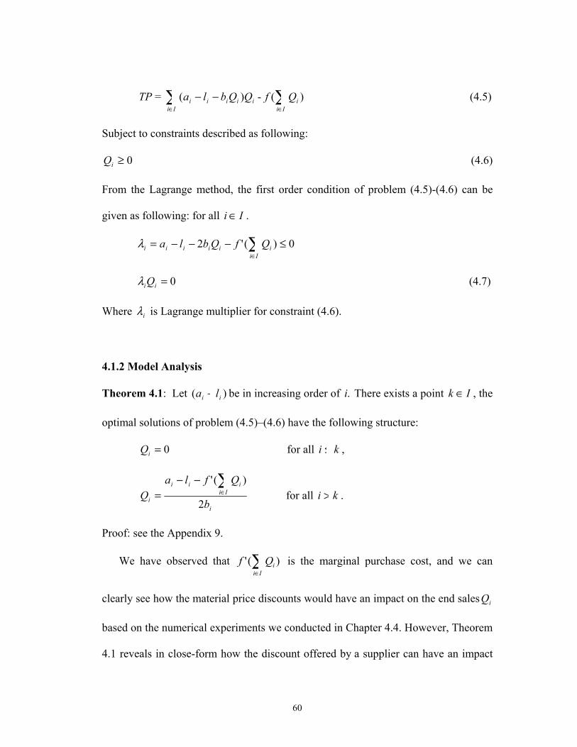
60
TP = ∑∈
−−Ii
iiiii QQbla )( - ∑∈Ii
iQf )( (4.5)
Subject to constraints described as following:
0≥iQ (4.6)
From the Lagrange method, the first order condition of problem (4.5)-(4.6) can be
given as following: for all Ii ∈ .
0)('2 ≤−−−= ∑∈Ii
iiiiii QfQblaλ
0=iiQλ (4.7)
Where iλ is Lagrange multiplier for constraint (4.6).
4.1.2 Model Analysis
Theorem 4.1: Let )( ii la − be in increasing order of .i There exists a point Ik ∈ , the
optimal solutions of problem (4.5)–(4.6) have the following structure:
0=iQ for all ki ≤ ,
i
Iiiii
i b
QflaQ
2
)(' ∑∈
−−= for all ki > .
Proof: see the Appendix 9.
We have observed that ∑∈Ii
iQf )(' is the marginal purchase cost, and we can
clearly see how the material price discounts would have an impact on the end sales iQ
based on the numerical experiments we conducted in Chapter 4.4. However, Theorem
4.1 reveals in close-form how the discount offered by a supplier can have an impact

61
on profit and purchased quantity. It will not only change the iQ ( ki > ), but it will
also change the iQ ( ki ≤ ). It gives us a formula, i.e. ∑∈
−−Ii
iii Qfla )(' , to identify
"profitable" and "non-profitable" demand, and only "profitable" demand will be
fulfilled and "non-profitable" demand will not be fulfilled -- a conclusion which is
different from the one shown in Chapter 4.4 because we don't have a "minimum fill
rate" constraint in this case. Furthermore, since material cost function )(⋅f is a
concave function, i. e. 0)(' <⋅f , the following applies: when the supplier offers
discount, )(' ⋅f decreases and iQ increases, which is in line with the one in Chapter
4.4. The other mechanism being investigated in Chapter 4.4 is offering of discount
on profitable products, or the equivalent of the following: If we reduce ib , then from
Theorem 4.1 iQ will increase, which is also in line with conclusion of Chapter 4.4:
Offering discount for profitable products will increase total purchased component
quantity.
From this Theorem we can have the following steps to derive the optimal iQ .
Algorithm:
Let ∑+=
−=
n
ki i
ii
bla
11 2
μ , ∑+=
=n
ki ib12 2
1μ .
Beginning
Step 1: Let 1=k
Step 2: Derive the MC by solving the equation: MCMCf =⋅− )(' 21 μμ
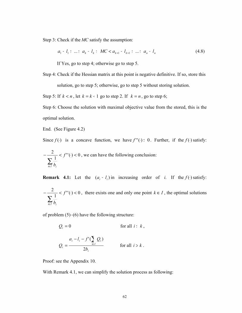
62
Step 3: Check if the MC satisfy the assumption:
nnkkkk lalaMClala −≤≤−<≤−≤≤− ++ ...... 1111 (4.8)
If Yes, go to step 4; otherwise go to step 5.
Step 4: Check if the Hessian matrix at this point is negative definitive. If so, store this
solution, go to step 5; otherwise, go to step 5 without storing solution.
Step 5: If nk < , let 1+= kk go to step 2. If nk = , go to step 6;
Step 6: Choose the solution with maximal objective value from the stored, this is the
optimal solution.
End. (See Figure 4.2)
Since )(⋅f is a concave function, we have 0)('' ≤⋅f . Further, if the )(⋅f satisfy:
0)(''1
2 <⋅<−∑∈
f
bIi i
, we can have the following conclusion:
Remark 4.1: Let the )( ii la − in increasing order of .i If the )(⋅f satisfy:
0)(''1
2 <⋅<−∑∈
f
bIi i
, there exists one and only one point Ik ∈ , the optimal solutions
of problem (5)–(6) have the following structure:
0=iQ for all ki ≤ ,
i
Iiiii
i b
QflaQ
2
)(' ∑∈
−−= for all ki > .
Proof: see the Appendix 10.
With Remark 4.1, we can simplify the solution process as following:
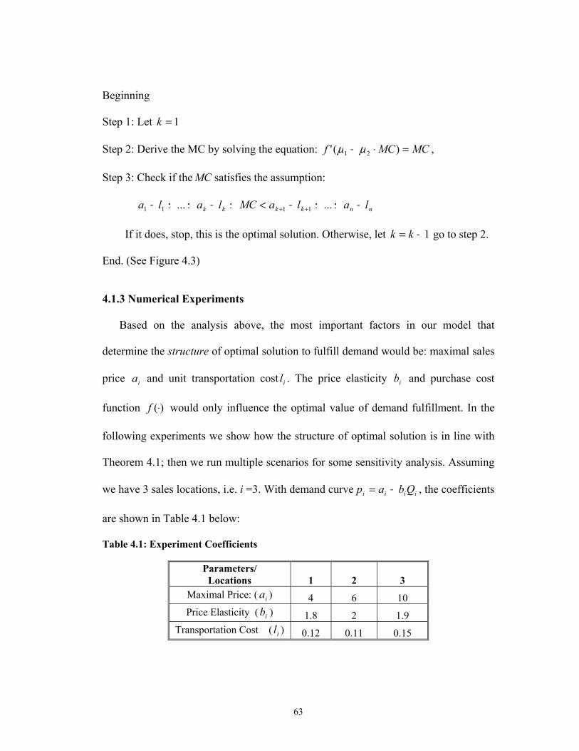
63
Beginning
Step 1: Let 1=k
Step 2: Derive the MC by solving the equation: MCMCf =⋅− )(' 21 μμ ,
Step 3: Check if the MC satisfies the assumption:
nnkkkk lalaMClala −≤≤−<≤−≤≤− ++ ...... 1111
If it does, stop, this is the optimal solution. Otherwise, let 1+= kk go to step 2.
End. (See Figure 4.3)
4.1.3 Numerical Experiments
Based on the analysis above, the most important factors in our model that
determine the structure of optimal solution to fulfill demand would be: maximal sales
price ia and unit transportation cost il . The price elasticity ib and purchase cost
function )(⋅f would only influence the optimal value of demand fulfillment. In the
following experiments we show how the structure of optimal solution is in line with
Theorem 4.1; then we run multiple scenarios for some sensitivity analysis. Assuming
we have 3 sales locations, i.e. i =3. With demand curve iiii Qbap −= , the coefficients
are shown in Table 4.1 below:
Table 4.1: Experiment Coefficients
Parameters/ Locations 1 2 3
Maximal Price: ( ia ) 4 6 10 Price Elasticity ( ib ) 1.8 2 1.9
Transportation Cost ( il ) 0.12 0.11 0.15
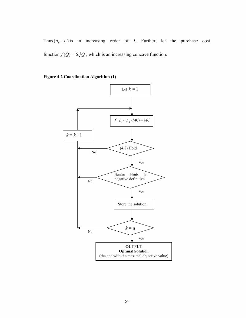
64
Thus )( ii la − is in increasing order of .i Further, let the purchase cost
function QQf 6)( = , which is an increasing concave function.
Figure 4.2 Coordination Algorithm (1)
Figure 4.2 Coordination Algorithm (1)
No
Yes
Let 1=k
(4.8) Hold
Yes
Store the solution
OUTPUT Optimal Solution
(the one with the maximal objective value)
Yes
No
No
MCMCf =⋅− )(' 21 μμ
Hessian Matrix isnegative definitive
k = n
k = k +1

65
Figure 4.3 Coordination Algorithm (2)
First, we solve the problem analytically (4.5 - 4.6) by Theorem 4.1 and algorithm
shown in Figure 4.2, the optimal solution is: ),( 3,21 QQQ = (0, 0, 2.05), the objective
function value (total profit) is 3.62. Now, let us examine the numerical experiments
to determine where our optimal solution stands in terms of the possible different
solution structures: (0, 0, 3Q ), (0, 2Q , 3Q ), ( 1Q ,0, 3Q ), ( 1Q , 2Q , 3Q ), which are
shown in Table 4.2 - 4.5 and the corresponding Figure 4.4 – 4.7 , respectively. Figure
4.4 clearly shows that as 3Q increases, total profit increases, but it begins to decline
beyond a certain value: 2.05. This occurs because, in order to have more demand, the
charged price has to be at a lower level. Note that after sales quantity reaches 2.05,
the additional profit can not offset the lost margin and increased transportation cost
anymore. Figure 4.5 – 4.7 show that if we increase 1Q or 2Q , or both from 0 to some
value without following Theorem 4.1, the total profit would indeed decrease. The
No Yes
Yes
Let 1=k
(4.8) Hold
MCMCf =⋅− )(' 21 μμ
k = n OUTPUT
Optimal Solution
k = k +1
No
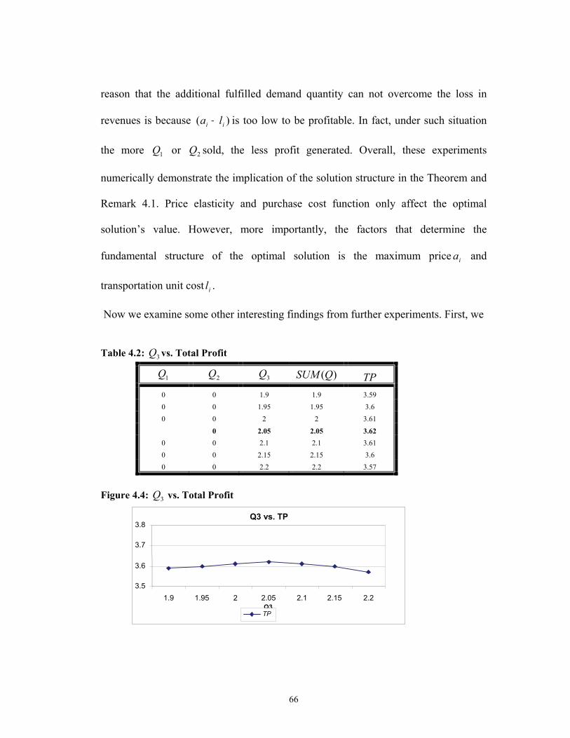
66
reason that the additional fulfilled demand quantity can not overcome the loss in
revenues is because )( ii la − is too low to be profitable. In fact, under such situation
the more 1Q or 2Q sold, the less profit generated. Overall, these experiments
numerically demonstrate the implication of the solution structure in the Theorem and
Remark 4.1. Price elasticity and purchase cost function only affect the optimal
solution’s value. However, more importantly, the factors that determine the
fundamental structure of the optimal solution is the maximum price ia and
transportation unit cost il .
Now we examine some other interesting findings from further experiments. First, we
Table 4.2: 3Q vs. Total Profit
1Q 2Q 3Q )(QSUM TP
0 0 1.9 1.9 3.59 0 0 1.95 1.95 3.6 0 0 2 2 3.61 0 2.05 2.05 3.62 0 0 2.1 2.1 3.61 0 0 2.15 2.15 3.6 0 0 2.2 2.2 3.57
Figure 4.4: 3Q vs. Total Profit
Q3 vs. TP
3.5
3.6
3.7
3.8
1.9 1.95 2 2.05 2.1 2.15 2.2Q3
TP

67
Table 4.3: 2Q , 3Q vs. Total Profit:
1Q 2Q 3Q )(QSUM TP
0 0 2.05 2.05 3.62 0 1.05 2.05 3.1 3.52 0 1.1 2.05 3.15 3.42
0 1.15 2.05 3.2 3.3 0 1.2 2.05 3.25 3.18 0 1.25 2.05 3.3 1.58 0 1.3 2.05 3.35 1.45
Figure 4.5: 2Q , 3Q vs. Total Profit
Table 4.4: 1Q , 3Q vs. Total Profit:
1Q 2Q 3Q )(QSUM TP
0 0 2.05 2.05 3.62
1.05 0 2.05 3.1 1.63
1.1 0 2.05 3.15 1.45
1.15 0 2.05 3.2 1.26
1.2 0 2.05 3.25 1.06
1.25 0 2.05 3.3 0.85
1.3 0 2.05 3.35 0.63
(Q2,Q3) vs. TP
0 1 2 3 4
2.05 3.1 3.15 3.2 3.25 3.3 3.35
Q2+Q3
TP
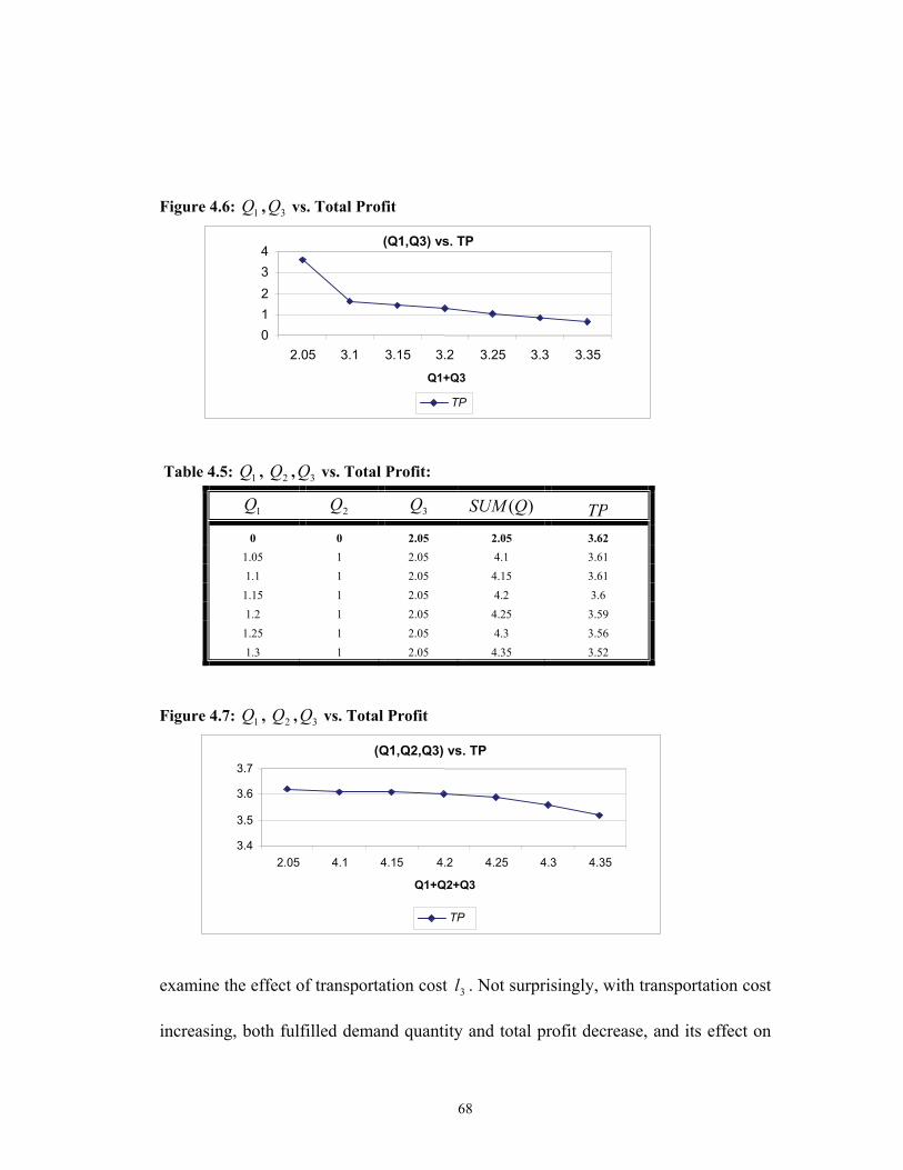
68
Figure 4.6: 1Q , 3Q vs. Total Profit
Table 4.5: 1Q , 2Q , 3Q vs. Total Profit:
1Q 2Q 3Q )(QSUM TP
0 0 2.05 2.05 3.62 1.05 1 2.05 4.1 3.61 1.1 1 2.05 4.15 3.61
1.15 1 2.05 4.2 3.6 1.2 1 2.05 4.25 3.59
1.25 1 2.05 4.3 3.56 1.3 1 2.05 4.35 3.52
Figure 4.7: 1Q , 2Q , 3Q vs. Total Profit
examine the effect of transportation cost 3l . Not surprisingly, with transportation cost
increasing, both fulfilled demand quantity and total profit decrease, and its effect on
(Q1,Q2,Q3) vs. TP
3.4
3.5
3.6
3.7
2.05 4.1 4.15 4.2 4.25 4.3 4.35
Q1+Q2+Q3
TP
(Q1,Q3) vs. TP
0 1 2 3 4
2.05 3.1 3.15 3.2 3.25 3.3 3.35
Q1+Q3
TP
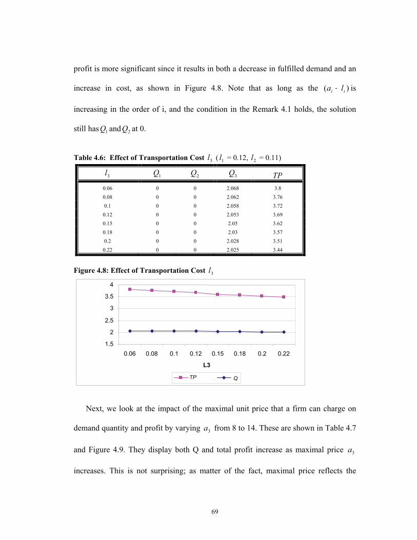
69
profit is more significant since it results in both a decrease in fulfilled demand and an
increase in cost, as shown in Figure 4.8. Note that as long as the )( ii la − is
increasing in the order of i, and the condition in the Remark 4.1 holds, the solution
still has 1Q and 2Q at 0.
Table 4.6: Effect of Transportation Cost 3l ( 1l = 0.12, 2l = 0.11)
3l 1Q 2Q 3Q TP
0.06 0 0 2.068 3.8 0.08 0 0 2.062 3.76 0.1 0 0 2.058 3.72
0.12 0 0 2.053 3.69 0.15 0 0 2.05 3.62 0.18 0 0 2.03 3.57 0.2 0 0 2.028 3.51
0.22 0 0 2.025 3.44
Figure 4.8: Effect of Transportation Cost 3l
Next, we look at the impact of the maximal unit price that a firm can charge on
demand quantity and profit by varying 3a from 8 to 14. These are shown in Table 4.7
and Figure 4.9. They display both Q and total profit increase as maximal price 3a
increases. This is not surprising; as matter of the fact, maximal price reflects the
1.5
2
2.5
3
3.5
4
0.06 0.08 0.1 0.12 0.15 0.18 0.2 0.22
L3
TP Q

70
customers’ desire and affordability of the product. Total profit increases more
significantly than Q due to the dual effects of raising both Q and price. Again, we
should notice that )( 33 la − in this scenario is always larger than
)( 11 la − and )( 22 la − , and in optimal solutions 1Q and 2Q remain at 0, which is exactly
as Theorem 4.1 points out.
Table 4.7: Effect of Maximal Price 3a ( 1a = 4, 2a = 6 )
3a 1Q 2Q 3Q TP
8 0 0 1.4 0.17 9 0 0 1.8 1.72 10 0 0 2.05 3.62 11 0 0 2.35 5.81 12 0 0 2.65 8.29 13 0 0 2.96 11.07 14 0 0 3.2 14.13
Figure 4.9: Effect of Maximal Price 3a
Table 4.8 and Figure 4.10 show the optimal solution of fulfilled demand quantity
and total profit as a function of price elasticity. For various levels as price elasticity,
3b , increases, both Q and total profit decrease, and profit decreases more steeply due
to the same dual effects as mentioned in maximal price discussion. Further, if we
0
5
10
15
8 9 10 11 12 13 14
A3
Q TP

71
compare Figure 4.8, 4.9 and 4.10, we can see that price-related coefficients, i. e.,
maximal price 3a and price elasticity 3b , have a more significant effect on profit than
transportation cost, does as evidenced by the “flat” curve in Figure 4.8 vs. “steep”
curve in Figure 4.9 and 4.10. This occurs because when end customers are buying
something, they are always more sensitive to visible price than transparent
transportation cost. In addition, in most cases, price accounts for a larger portion of
the cost than the transportation cost itself. Thus the firm should carefully determine
the quantity of demand to fulfill as demonstrated in Theorem 4.1 and shown in the
results above. Fulfilling more demand doesn’t necessarily mean more profit is
secured. Sometimes it may even hurt the business.
Table 4.8: Effect of Price Elasticity’s 3b ( 1b =1.8, 2b = 2 )
3b 1Q 2Q 3Q TP
1.6 0 0 2.49 5.14 1.7 0 0 2.32 4.56 1.8 0 0 2.18 4.06 1.9 0 0 2.05 3.62 2 0 0 1.92 3.22
2.1 0 0 1.82 2.88 2.2 0 0 1.72 2.56
Figure 4.10: Effect of Price Elasticity’s 3b
1.52
2.53
3.54
4.55
5.5
1.6 1.7 1.8 1.9 2 2.1 2.2
B3
Q TP
72
4.2 Analytical Model with Stochastic Demand In Section 4.1, we assumed that the demand is price-dependent with different
demand curves at each sales location. Therefore no inventory cost is considered. This
scenario is true as stated in the theory of monopolistic competition (Chamberlain and
Robinson 1954), where the demand curve of a monopoly firm is downward sloping
and the inventory will not be an issue when price can be used as a decision tool.
However, if one company did not posses the monopolistic power, e.g., under
fierce global competition, it has to face the uncertainty of customer demand. In such
cases, inventory holding to support sales becomes significant. Effectively managing
and minimizing the inventory holding cost while satisfying customer demands could
provide a competitive advantage to any firm in the marketplace. Besides the
inventory cost, we also take into account the lost sales (supply shortage) penalty that
would be incurred when demand can not be met. We further assume that the uncertain
demand on each path can have different distributions. The fundamental decision in
this constrained stochastic model is still to derive an optimal purchase quantity for the
raw materials and a sales quantity for the end products in every location to maximize
the profit of the company.
A body of literature closely related to this topic is newsvendor-like problems,
which are to find the order quantity which maximizes the expected profit in a single-
period probabilistic demand framework. By assuming that the retailers’ demand
obeys a normal or lognormal distribution and that the retailers place orders according
to the Newsvendor Rule, researchers derive the necessary and sufficient conditions

73
for the optimal solution of production size (Khouja, 2000; Z.Weng 2003). Our model
differs from theirs on: 1) It is more generalized and all demands are equally treated;
(Unlike Cattni (2000)’s paper, we don’t need hierarchical priority in the model.) 2) it
can be applied to any unknown-but-bounded disturbances; 3) with both manufacturers
and retailers in the picture, it is a constrained stochastic problem.
We also would like to point out that this model is different from a multi-inventory
system. Most papers that have discussed multi-inventory systems have assumed that
the retailer’s ordering policy is only related to the demand and supplier but unrelated
to the other retailers. Some supply-chain and inventory models use the following two-
echelon symmetric-information and deterministic gaming structure: a
‘‘manufacturer’’ wholesales a product to a ‘‘retailer,’’ who in turn retails it to the
consumer. The retail market demand varies either with the retail price according to a
deterministic ‘‘demand function’’ that is known to both the manufacturer and the
retailer or with the known distribution. The manufacturer is a Stackelberg leader and
the retailer is a Stackelberg follower (from Franco Blanchini etc. 2004). Thus they
completely separate the “market channel” from “manufacturing channel” to make
decisions. Under the approach described, in the next section, we derive an optimal
promising policy from a centralized supply chain’s point, in which the company
considers the “market channel” and “manufacturing channel” together as a path.
4.2.1 Model & Formulation
The problem under consideration is a single time period, single product, two-
echelon supply chain system. As before, we assume there is one supplier and n sales

74
locations. The manufacturer buys raw materials from the supplier, and after
assembling, sells finished products to end-customers via sales locations. In practical
situations, the supplier usually offers price discounts to manufactures if their purchase
quantity increases and therefore total purchase cost is concave (the cost function is
denoted by )(⋅g ). The supply chain path is the path from one manufacturer to sales
location (Figure 4.11). Let { }NI ,,2,1 L= be the index set of the sales locations. For
all Ii ∈ , let the path unit cost be il and the demand of each market as iu , which is a
random variable with known probability density function (PDF) denoted by )(⋅f and
c. d. f. denoted by )(⋅F . ip is the sales price in each market. We assume one raw
material unit per finished product unit.
Our decision variables are:
Q : the raw material purchase quantity.
iS : the quantity of finished product sold at location .i
Figure 4.11 Supply Chain Path (2)
Price: pi Demand: ui Holding : hi
Sales Location
li
g (Q) Supplier

75
Formulation:
Revenue: ),min( iii
i uSp∑ = ∑ ∫∫∞
+i
iiS
i
S
iiii duufSduufupi
i
))()((0
Purchase Cost: )(Qg , )(⋅g is a concave function Transportation Cost: ∑
iii Sl
Holding Costs on sales location:
∑ −×i
iii uSh )0,max( = ])()([0
iiii
S
ii duufuShi
−∑ ∫
Shortage Cost: ∑ −×i
iii Sud )0,max( = ])()([ iiiii S
i duufSudi
i
−∑ ∫∞
We would like to: Maximize:
Profit = Revenue - Purchase Cost - Transportation Cost - Holding Costs – Shortage
cost
So the problem now is:
Max: ∑ ∫∫∞
+i
iiS
i
S
iiii duufSduufupi
i
))()((0
- )(Qg - ∑i
ii Sl - ])()([0
iiii
S
ii duufuShi
−∑ ∫ -
])()([ iiiii S
i duufSudi
−∑ ∫∞
s. t. 0≥− ∑
iiSQ
0≥iS , 0≥Q It is equivalent to:

76
Min: ii
S
i iiiiiiii
iiii SldpSgduufuSdhp
i
)()()()()(0
−+−+−++ ∫ ∑ ∑∑ (4.9)
s. t. 0≥iS (4.10)
4.2.2 Model Analysis
From the Lagrange method, the first order condition of this problem can be given
as the following: Kuhn-Tucker condition for all Ii ∈ .
0)()()()( '' ≥−+−+++= ∑ iiii
iiiiiii ldpSgSWhdpλ (4.11)
0=ii Sλ
0≥iλ
)( ii SW is defined by +− ][ iii uSE = ∫ −iS
iiii duufuS0
)()( . Assume )(⋅iW is everywhere
differentiable, we have: )()(' iii SFSW = . It’s easy to show: 0)0()0( ' == ii WW , and
)(⋅iW is convex (see Appendix 11).
Theorem 4.2: Let the )( iii ldp −+ in increasing order of .i There exists a point
Ik ∈ such that the optimal solutions of problem (4.9)–(4.10) has the following
structure:
0=iS for all ki ≤ , (4.12)
iii
Iiiiii
i hdp
SgldpSF
++
−−+=
∑∈
)(')()( for all ki > . (4.13)
Proof: see Appendix 12.

77
We can further show that an upper bound exists for Q (see Appendix 13), which
reveals that, even with a discount on raw material, it would not be foolish to limit the
total quantity purchased. Unsurprisingly, the transportation cost il , shortage penalty
id and sales price ip have an impact on the decision. Also, we notice that ∑∈Ii
iSg )('
can be interpreted as the marginal purchase cost. From Theorem 4.2 we can easily
see it is a decisive factor of the end sales iS . Another interesting finding is that
inventory cost ih has no effect at the first stage where we determine whether the
finished product should be sold at one location or not. It only plays a role at the
second stage where we determine the sold quantity iS (for ki > ).
4.2.3 Algorithm:
BEGIN:
Step 1: Let 1=k
Step 2: Derive the iS by solving the equations (4.12)-(4.13).
Step 3: Check if the ∑i
iSg )(' satisfy the assumption:
nnnkkki
ikkk ldpldpSgldpldp −+≤≤−+<≤−+≤≤−+ +=+∑ ...)('... 111111
(4.14)
If so, go to step 4; otherwise go to step 5.
Step 4: Check if the Hessian matrix at this point is negative definitive. If so, store
this solution, go to step 5; otherwise, go to step 5 without storing.
Step 5: If nk < , let 1+= kk go to step 2. If nk = , go to step 6;

78
Step 6: Choose the solution with maximal objective value from the stored, this is the
optimal solution.
END. (see the Figure 4.12)
Remark 4.2: Let the )( iii ldp −+ be increasing .i If
UGUFdhpi iii
×>++∑ )(
1
where UF and UG is the upper bound of )(⋅f and )('' ⋅− g respectively, then there
exists a unique Ik ∈ for which the optimal solutions of problem (4.9) – (4.11) have
the following structure:
0=iS for all ki ≤ ,
iii
Iiiiii
i hdp
SgldpSF
++
−−+=
∑∈
)(')()( for all ki > .
Proof: see the Appendix 14.
Using Remark 4.2, we can state the following simplified algorithm:
Algorithm 2:
BEGIN:
Step 1: Let 1=k
Step 2: Derive the iS by solving the equations (4.12)-(4.13).
Step 3: Check if the ∑i
iSg )(' satisfy the assumption:
nnnkkki
ikkk ldpldpSgldpldp −+≤≤−+<≤−+≤≤−+ +=+∑ ...)('... 111111

79
If so, Stop; Otherwise, let 1+= kk go to step 2.
END. (see the Figure 4.13)
Figure 4.12. Coordination Algorithm (3)
No
Yes
No
k = k +1
Let 1=k
Store the solution
OUTPUT Optimal Solution
(the one with the maximal objective value) function
Yes
Hessian Matrix isnegative definitive
k = n
Solve Equations (4.12-4.13)
Yes
No
∑≤−+ )( ikkk Sgldp
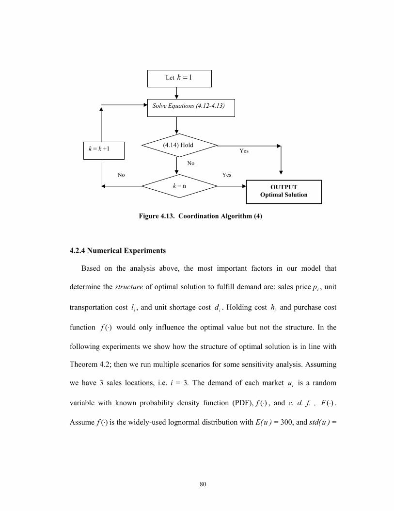
80
Figure 4.13. Coordination Algorithm (4)
4.2.4 Numerical Experiments
Based on the analysis above, the most important factors in our model that
determine the structure of optimal solution to fulfill demand are: sales price ip , unit
transportation cost il , and unit shortage cost id . Holding cost ih and purchase cost
function )(⋅f would only influence the optimal value but not the structure. In the
following experiments we show how the structure of optimal solution is in line with
Theorem 4.2; then we run multiple scenarios for some sensitivity analysis. Assuming
we have 3 sales locations, i.e. i = 3. The demand of each market iu is a random
variable with known probability density function (PDF), )(⋅f , and c. d. f. , )(⋅F .
Assume )(⋅f is the widely-used lognormal distribution with E(u ) = 300, and std(u ) =
YesNo
Yes
Let 1=k
(4.14) Hold
k = n OUTPUT Optimal Solution
k = k +1
No
Solve Equations (4.12-4.13)

81
60. In addition, let the purchase cost function QQf 6)( = , which is an increasing
concave function. The other coefficients are shown in Table 4.9 below:
Table 4.9: Experiment Coefficients Parameters/
Locations 1 2 3 Sales Price: ( ip ) 4 8 10
Transportation Cost ( il ) 0.7 0.8 0.9 Holding Cost ( ih ) 0.2 0.25 0.4
Shortage Cost ( id ) 0.5 0.8 1 First, we solve the problem analytically (4.9 - 4.11) by Theorem 4.2 and using the
algorithm shown in Figure 4.12 yields the optimal solution: ),( 3,21 SSS = (0, 0, 198),
with objective function value (total profit) 762. Like the experiments shown in Table
4.2 - 4.5, the solution structure has exactly the same form as Theorem 4.2 and
Remark 4.2, since in our case )( iii ldp −+ is in increasing order of .i In addition, it is
confirmed numerically that the purchase cost function and holding cost only affect the
optimal solution’s value. Most importantly, the sales price ip , transportation cost il
and shortage cost id determine the fundamental structure of the optimal solution.
Now let us examine some interesting findings from the following experiments.
First, we investigate the effect of varying the demand mean. Unsurprisingly, as the
mean of demand increases, both fulfilled demand quantity and total profit increases,
its effect on profit is more significant since it results in both sales increase and
purchase cost decrease due to economies of scale, as shown in Figure 4.14. Note that
as long as )( iii ldp −+ is increasing in the order of i, and the condition of Remark 4.2
holds. 1S and 2S will remain at 0.

82
Table 4.10: Effect of Demand’s Mean (STD = 60)
AVG 1S 2S 3S )( iSsumQ = TP
297 0 0 170 170 684 300 0 0 198 198 762 317 0 0 205 205 886 328 0 0 224 224 932 380 0 0 296 296 1013
Figure 4.14: Effect of Demand’s Mean
Next, we look at the impact of demand’s standard deviation on fulfilled demand
quantity and profit by varying std from 30 to 150. These are shown in Table 4.11
and Figure 4.15. They show that the fulfilled demand quantity increases, while the
total profit decreases as the standard deviation of demand increases. This can be
explained as follows: large variance in demand patterns create havoc for a company,
which in turn must sell more quantity to offset it. Even so, the generated revenues are
still not enough to overcome the loss due to overstocking (holding cost) and lost sales
(shortage cost). Thus, accurate demand forecasts are a business imperative. After all,
the better you can match supply with actual demand, the more streamlined your
business operations will be. Thus, a company needs the capability to track forecast
accuracy in real-time, allowing management to take immediate action to eliminate
forecast errors and improve the overall demand forecasting process.
100 300 500 700 900
1100 1300
297 300 317 328 380Mean of Demand
TP S3, Q

83
Again, we should notice that )( 333 ldp −+ in this scenario is always larger than
)( 111 ldp −+ and )( 222 ldp −+ , and in optimal solutions 1S and 2S stay at 0, which is
exactly what Theorem 4.1 points out.
Table 4.11: Effect of Demand’s Stand Deviation (AVG = 300)
STD 1S 2S 3S )( iSsumQ = TP
30 0 0 191 191 778 60 0 0 198 198 762 90 0 0 216 216 746
120 0 0 237 237 722 150 0 0 263 263 688
Figure 4.15: Effect of Demand’s Stand Deviation
For various levels of transportation cost 3l , as 3l increases (Table 4.12), both Q
and total profit monotonically decrease. This result is obvious as the company is
increasingly more costly now, profits decrease more steeply (Figure 4.16) due to the
dual effects from increased cost and reduced fulfilled quantity. We also notice that
2S changes from 0 to 142 when 3l increases to 3.2. This should not surprise us as,
according to Theorem 4.2, the break point for )( 333 ldp −+ in this scenario is 3l =
3.0. In addition, even the optimal value of 2S changes, the solution structure still
observes the formula (4.12) and (4.13).
100 300 500 700 900
30 60 90 120 150
STD of Demand
TP S3,Q
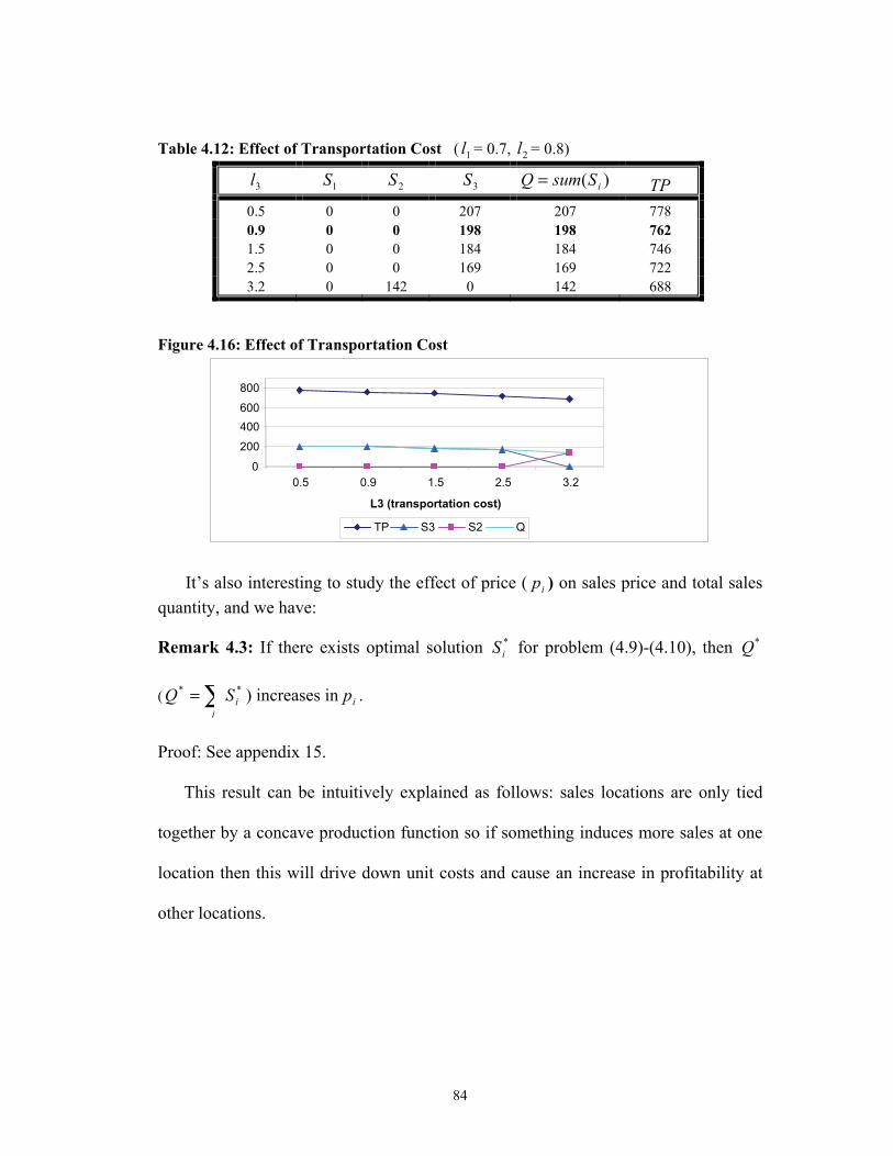
84
Table 4.12: Effect of Transportation Cost ( 1l = 0.7, 2l = 0.8)
3l 1S 2S 3S )( iSsumQ = TP
0.5 0 0 207 207 778 0.9 0 0 198 198 762 1.5 0 0 184 184 746 2.5 0 0 169 169 722 3.2 0 142 0 142 688
Figure 4.16: Effect of Transportation Cost
It’s also interesting to study the effect of price ( ip ) on sales price and total sales quantity, and we have: Remark 4.3: If there exists optimal solution *
iS for problem (4.9)-(4.10), then *Q
( ∑=i
iSQ ** ) increases in ip .
Proof: See appendix 15.
This result can be intuitively explained as follows: sales locations are only tied
together by a concave production function so if something induces more sales at one
location then this will drive down unit costs and cause an increase in profitability at
other locations.
0 200 400 600 800
0.5 0.9 1.5 2.5 3.2
L3 (transportation cost)
TP S3 S2 Q

85
4.3 Analytical Model for Balanced Supply Competition becomes stiffer and margins get smaller. Globalization, more
demanding customers and shortened product lifecycles are challenges in today’s
competition. Companies are continuously forced to improve their performance in
order to create value-added (VA) to customers from day to day, if they want to
remain profitable. As companies continuously seek to provide their products and
services to customers faster, cheaper, and better than their competitors, they realized
that they cannot do it without considering the “product path”. From supply chain’s
perspective, this means that products have to reach the customers from the right
supplier. Supply chain diversity ranges from globally dispersed manufacturers,
distribution centers and sales subsidiaries with different production cost, capacities,
capabilities and lead-times for different products. Therefore identifying the right
supplier/path is crucial for effective order promising, capacity utilization and
production smoothness. Overcoming the diminishing profit margin and achieving the
resource allocation efficiency stimulates us to do path analysis for the global supply
chain. Again, when we say product path, we refer to the path from the supplier where
the raw materials are purchased to manufacturer where products are produced,
through the distribution center (D.C.), and to the sales locations where the products
are finally sold to the customers.

86
In previous section we stated that, to counteract price erosion and the resulting
reduction in profit margin, manufacturers need to align the production and logistics
planning with the end-sales to choose the right path. Especially, in such a risky and
uncertainty environment, from the purchasing of raw material to manufacturing, to
the D.C, and finally to the customer, companies have to use different suppliers in
order to avoid vulnerability in market competition and reduce risk (L.Hunter 2004).
This brings us our major concern: the “balanced supply”. To meet customer demand,
decision-makers on the supply side include suppliers, manufacturers and distributors.
They are concerned not only with profit maximization but also with risk minimization
(A. Nagruney 2004). At the same time, developing more responsive strategies
requires multiple suppliers to respond to different supply chain drivers. One of the
time-based competition strategies proposed by D. Kritchanchaj (1999). focuses on
how to improve flexibility and responsiveness of business processes to meet customer
requirements. Organizations need to ensure that they continually monitor the
changing demands of customers and then attempt to meet their customer's
expectations in order to defend their market position against competitors. The
capability of responding quickly to customers’ demand is a key business process. But
the bottom line is the responsiveness of different suppliers varies. Hence, meeting
customer demands with different suppliers instead of adopting only one supplier, thus
has become a prerequisite for business survival in the face of market globalization
where rapidly changing business environments and seemingly insatiable customer
expectations have become the norm. This is especially true for companies that incur
the burden of high logistics costs. For example, Amazon.com has at least 2 fulfillment

87
centers to cover any customer zone in order to satisfy its trademark “shipping
guarantee policy”. Achieving this feat during Christmas season is paramount for any
retailer. All these point us in one direction: reducing the risk through balanced supply.
4.3.1 Model & Formulation
The problem under consideration below is a single time period, single product,
multiple-tier supply chain model. In particular, we consider one focal company with
multiple suppliers, which provide the material to manufacturing sites / distribution
sites. The manufacturing sites are involved in the production of a homogeneous
product which is then shipped to distributors, who, in turn, ship the product to end
customers. To simplify the deriving process, the supply chain path is illustrated to be
from one supplier to one sales location. (See Figure 4.17). The fundamental decision
in the model is to decide the optimal supply of products from each supplier to meet
the end customer’s demand so that the profit of the company is maximized, while
supply balance is also achieved. This problem is modeled as a constrained non-linear
integer programming problem.
4.3.1.1 Inputs
• Set F of Suppliers, I = n. In general elements of I will be identified by i.
• Customer demand Q : a given quantity.
• Unit cost iC : This represents linear cost such as materials needed
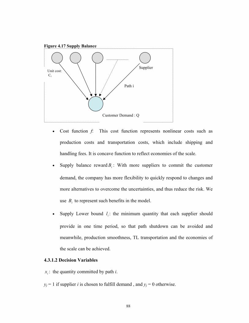
88
Figure 4.17 Supply Balance
• Cost function f: This cost function represents nonlinear costs such as
production costs and transportation costs, which include shipping and
handling fees. It is concave function to reflect economies of the scale.
• Supply balance reward iB : With more suppliers to commit the customer
demand, the company has more flexibility to quickly respond to changes and
more alternatives to overcome the uncertainties, and thus reduce the risk. We
use iB to represent such benefits in the model.
• Supply Lower bound il : the minimum quantity that each supplier should
provide in one time period, so that path shutdown can be avoided and
meanwhile, production smoothness, TL transportation and the economies of
the scale can be achieved.
4.3.1.2 Decision Variables
ix : the quantity committed by path i.
yj = 1 if supplier i is chosen to fulfill demand , and yj = 0 otherwise.
Path i
Unit cost: Ci
Supplier
Customer Demand : Q

89
In other words: yi = 1 if ix >0,
yi = 0 if ix = 0.
4.3.1.3 Model
Minimize ∑∑ −+i
iii
iii yBxCxf ))(( (4.15)
Subject to:
∑ =i
i Qx (4.16)
yi = 1 if ix >0,
yi = 0 if ix = 0. (4.17)
ii lx ≥ if ix >0 (4.18)
We can see, (4.17) and (4.18) are equivalent to: if ,1=iy then ii lx ≥ ; if ,0=iy
then 0=ix , which can be expressed as:
ii yMx ⋅≤
iii ylx ⋅≥
0≥ix
1,0=iy
and the model can be simplified as:
Min ∑∑ −+i
iii
iii yBxCxf ))(( (4.19)
subject to:
∑ =i
i Qx (4.20)
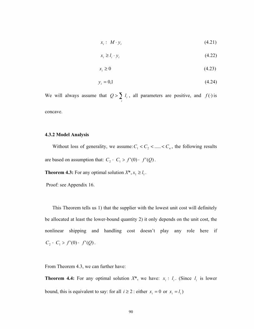
90
ii yMx ⋅≤ (4.21)
iii ylx ⋅≥ (4.22)
0≥ix (4.23)
1,0=iy (4.24)
We will always assume that ∑>i
ilQ , all parameters are positive, and )(⋅f is
concave.
4.3.2 Model Analysis
Without loss of generality, we assume: nCCC <<< .....21 , the following results
are based on assumption that: )(')0('12 QffCC −>− .
Theorem 4.3: For any optimal solution X*, 11 lx ≥ .
Proof: see Appendix 16.
This Theorem tells us 1) that the supplier with the lowest unit cost will definitely
be allocated at least the lower-bound quantity 2) it only depends on the unit cost, the
nonlinear shipping and handling cost doesn’t play any role here if
)(')0('12 QffCC −>− .
From Theorem 4.3, we can further have:
Theorem 4.4: For any optimal solution X*, we have: ii lx ≤ . (Since il is lower
bound, this is equivalent to say: for all 2≥i : either 0=ix or ii lx = )
91
Proof: see Appendix 17.
These Theorems give us a clear and simple solution. It shows us that the first
supplier is used at 1l and for all the other suppliers, the solution space is not infinite
but a very limited number of possibilities.
From Theorem 4.3 and Theorem 4.4, we can see that, without any complicated
assumptions and constraints involved, this model provides a simple structure relative
to demand fulfillment and balanced utilization of the supply chain. The model’s
conclusion can also be broadly applied to other similar situations.
4.4 Available Resource Analysis Identifying profitable paths is also a powerful weapon coordinating an available
resource such as component inventory or capacity, with order management (sales
subsidiaries) policies because it enables a company to know which path is profitable
and therefore can improve the customer service at least cost. The path in the real-life
global supply chain is difficult to handle analytically since they involve interactions
among several individual factors as well as thousands of products and product
locations. To reduce complexities and improve insight, we create an aggregate level
model, which means sales subsidiaries, rather than the individual orders, are the unit
of attention.

92
In the research below we study the firm’s optimal response to a price discount on
a component (raw material) under two different strategies. In the first strategy, the
firm does not pass along the discount to its customers (sales subsidiaries); the firm
simply coordinates sales among the different products and subsidiaries to minimize
the financial impact of non–profitable products. In the second strategy, the firm
offers price discounts in different sales subsidiaries to increase the demand for
profitable products. We carried out experiments for the two strategies based on a
mathematical programming model, built around Toshiba’s global notebook supply
chain. Model constraints include, among others, material constraints, bill–of–
materials, capacity and transportation constraints, and a constraint on minimum fill
rate (service level constraint). Unlike most models of this type in the literature, which
define variables in terms of single arc flows, we employ path variables, which allow
for direct direction identification and manipulation of profitable and non–profitable
products.
4.4.1 Model background Facing fierce competition, many companies have to cope with two conflicting
goals: one is to maximize total profit; the other one is to maintain a high level of
service, usually measured by fill–rate. For strategic reasons, a firm may set a lower
bound on its fill rate, be it global (across products and locations), or local for a given
location. This constraint usually forces a company to sell non–profitable products.
Meantime, due to the different path involved, similar products might be profitable in
one path (location) but non-profitable in the other. In this study, we consider n
93
products, which are variations of a generic product, and can be thought of as
configurations for a notebook PC. The products are manufactured in different
factories at different costs, and sold in different sales subsidiaries, also called sales
locations, at different prices.
Temporary price discounts by suppliers are a relatively common phenomenon––
these occur as a result of supply–demand imbalances (e.g., production overruns, poor
forecasting, etc.), competition among suppliers, retooling, etc. (Tersine and Barman
1995). In this research we consider the issue of coordinating available resource with
sales at different locations in a global, capacitated, sourcing–manufacturing–
distribution supply chain under such temporary price discount. This research is based
on a two–year project conducted with Toshiba Corporation. All products have a
common and critical component, for which the supplier offers a price discount in one
time period.
Customers are price–sensitive and demand for a product is assumed to decrease
linearly with its price. We define a sales subsidiary’s fill rate as total committed
quantity divided by its total demand. There are different minimum fill rate
requirements across different sales subsidiaries. This minimum fill rate requirement
may induce sales products that are non–profitable in that location. We propose two
coordinating mechanisms to improve the resource utilization and reduce the financial
impact of non–profitable products. The first mechanism simply buys a large amount
of components at the discounted price to use them in non–profitable products for as
long as possible––the length of time is related to inventory holding costs, and
capacity considerations along the chain (transportation, production, etc.). An optimal

94
procurement quantity trades off gains from the discounted price against additional
holding costs, taking into account the various capacity constraints. The second
mechanism reduces the quantity of non–profitable products needed to meet the
minimum service level constraint by increasing sales of profitable products via a price
discount. Note that offering price discounts for profitable products has the potential
of increasing profits due to two effects: increased demand, and decreased sales of
non–profitable products, however, too large a price discount can ultimately hurt
profits by decreasing total revenue. We should point out here, without the product
path to identify profitable product, such coordinating mechanism is impossible to be
carried out.
4.4.2 Toshiba Supply Chain In this section we model Toshiba’s notebook (PC) global supply chain (Figure
4.18), which comprises four final assembly and testing (FAT) factories and six sales
subsidiaries, including locations in Japan, The Philippines, United States and
Germany. Toshiba buys PC components, including CPU, hard disk drive, keyboard,
LCD, CD–ROM, and DVD–ROM, directly from suppliers, and transports the
motherboard subassembly from subassembly factories; these are shipped to the FAT
factories for assembly, and finished PCs are finally shipped to the different sales
subsidiaries. The motherboard components are bought from suppliers, and all
subassembly factories can produce all types of motherboards. There are over 3,500
different product models offered across the different sales subsidiaries. Although our

95
model is based on Toshiba Corporation, it is clear that the structure of its supply chain
is similar to many other firms operating in similar industries.
SupplierSingapore
SupplierJapan
Japan FAT
Philippine FAT
USA FAT
Germany FAT
SalesAustralia
SaleCanada
SalesSingapore
SalesJapan
SalesUSA
SubsidiariesIn Europe
Customer
Customer
Customer
Customer
Customer
Customer
SupplierGerman
Suppliers FAT Sales
Figure 4.18 Toshiba Global Supply Chain Our sourcing–production–distribution planning model spans a time horizon of 13
weeks. Unmet demand for a sales subsidiary at any period cannot be backordered;
consequently committed quantity is equal or lower than demand. The supplier
network is not considered in this model and thus we ignore holding costs at the
suppliers. The integrated supply chain model is a multi–period, multi–echelon and
multi–product MIP model (integer variables are necessary because of minimum lot
size requirements), which is presented in §4.4.3
From a modeling perspective, our global supply chain model is rather
straightforward, except for a choice in the decision variables, which allows us to
answer the research questions posed in §4.4.1. As explained in the Chapter 1, unlike

96
most models in the global supply chain literature, which define variables in terms of
flows along a single arc in the network and use flow balancing constraints at nodes,
we employ path variables, which provide location–specific cost information and
directly identify profitable and non–profitable products In our two–year research
project with Toshiba, we found this to be very important managerial information, as it
serves as an aid for other strategic decisions such as product line offering at different
locations. Although this modeling approach certainly increases the number of
decision variables (for example, a typical model we study here has over a million
variables and a similar number of constraints), we find that the resulting models, even
with real–world data, are manageable with solution times being around 5 minutes
using typical computing environments.
4.4.3 Model Formulation Notation Index Use (Indices and Index Sets)
s S∈ Sales subsidiaries
f F∈ Final assembly and testing (FAT) factories
l L∈ Subassembly factories.
i I∈ Product (notebook PC models)
j J∈ Components sourced directly from suppliers
j J∈ Motherboard (sourced from subassembly factories)
k K∈ Motherboard components.
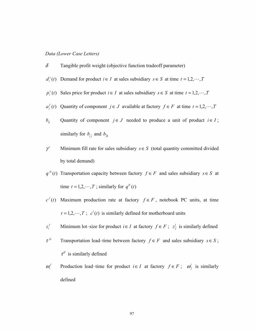
97
Data (Lower Case Letters)
δ Tangible profit weight (objective function tradeoff parameter)
)(td si Demand for product Ii ∈ at sales subsidiary Ss ∈ at time Tt ,,2,1 L=
)(tp si Sales price for product Ii ∈ at sales subsidiary Ss ∈ at time Tt ,,2,1 L=
( )fja t Quantity of component Jj ∈ available at factory f F∈ at time Tt ,,2,1 L=
ijb Quantity of component Jj ∈ needed to produce a unit of product Ii ∈ ;
similarly for i jb and jkb
sγ Minimum fill rate for sales subsidiary s S∈ (total quantity committed divided
by total demand)
)(tq fs Transportation capacity between factory f F∈ and sales subsidiary s S∈ at
time Tt ,,2,1 L= ; similarly for ( )lfq t
( )fc t Maximum production rate at factory f F∈ , notebook PC units, at time
Tt ,,2,1 L= ; ( )lc t is similarly defined for motherboard units
fiz Minimum lot–size for product i I∈ at factory f F∈ ; l
jz is similarly defined
fsτ Transportation lead–time between factory f F∈ and sales subsidiary s S∈ ;
lfτ is similarly defined
fiω Production lead–time for product i I∈ at factory f F∈ ; l
jω is similarly
defined

98
fjr Unit purchasing cost of component j J∈ at factory f F∈ at time
Tt ,,2,1 L= ; lkr is similarly defined
sih Unit holding cost for product i I∈ at sales subsidiary s S∈ ; l
kh , fjh are
similarly defined
fiv Production cost per unit for product i I∈ at factory f F∈ ; l
jv is similarly
defined
fsw Transportation cost per unit between FAT factory f F∈ and sales subsidiary
s S∈ , including taxes or duties; lfw is similarly defined.
Path Decision Variables (capital letters)
( )lfsiD t Quantity of product i I∈ produced at factory f F∈ by using motherboard
from sub–assembly factory l L∈ and shipped to sales subsidiary Ss ∈ at
time Tt ,,2,1 L=
Auxiliary Variables (Capital Letters)
( )siM t Demand commitment for product i I∈ at sales subsidiary Ss ∈ at time
Tt ,,2,1 L=
( )fiQ t Quantity of product i I∈ produced at factory f F∈ at time Tt ,,2,1 L= ;
( )ljQ t is similarly defined

99
( )fiZ t Binary variable (= 1, if product i I∈ is produced at factory f F∈ at time
Tt ,,2,1 L= ; 0 otherwise); ( )ljZ t is similarly defined
)(tH si Inventory on hand for product i I∈ at sales subsidiary Ss ∈ at time
Tt ,,2,1 L= ( (0)siH is known and given); ( )f
jH t and ( )lkH t are similarly
defined
)(tC si Total cost for product i I∈ sold at sales subsidiary Ss ∈ at time Tt ,,2,1 L=
)(tP si Total profit for product i I∈ sold at sales subsidiary Ss ∈ at time
Tt ,,2,1 L=
( )C t% Total PC component and motherboard component holding cost at time
Tt ,,2,1 L=
The objective function maximizes profit––revenue from promised orders minus
transportation, production, duty, component, and inventory costs. Constraints
include: demand commitment and fill rate constraints, inventory balance constraints
at factories and sales subsidiaries, minimum lot size, and production and
transportation capacity constraints.
Objective function: maximize profit
1
max ( )T s s
it i
P t=∑ ∑ (4.25)
Subject to:
Demand commitment and minimum fill rate constraints
( ) ( ) , 1 ,s si iM t d t i I t T≤ ∈ ≤ ≤ (4.26)
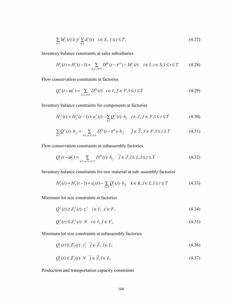
100
( ) ( ) , 1 ,s s si i
i I i IM t d t s S t Tγ
∈ ∈≥ ∈ ≤ ≤∑ ∑ (4.27)
Inventory balance constraints at sales subsidiaries
,
( ) ( 1) ( ) ( ) , ,1s s lfs fs si i i i
l L f FH t H t D t M t i I s S t Tτ
∈ ∈= − + − − ∈ ∈ ≤ ≤∑ (4.28)
Flow conservation constraints at factories
,
( ) ( ) , ,1f f lfsi i i
l L s SQ t D t i I f F t Tω
∈ ∈− = ∈ ∈ ≤ ≤∑ (4.29)
Inventory balance constraints for components at factories
( ) ( 1) ( ) ( ) , ,1f f f fj j j i ij
i IH t H t a t Q t b j J f F t T
∈= − + − ⋅ ∈ ∈ ≤ ≤∑ (4.30)
, ,
( ) ( ) , ,1f lfs lfi ii j i j
i I i I s S l LQ t b D t b j J f F t Tτ
∈ ∈ ∈ ∈⋅ = − ⋅ ∈ ∈ ≤ ≤∑ ∑ (4.31)
Flow conservation constraints at subassembly factories
, ,
( ) ( ) , ,1l l lfsij j i j
i I s S f FQ t D t b j J l L t Tω
∈ ∈ ∈− = ⋅ ∈ ∈ ≤ ≤∑ (4.32)
Inventory balance constraints for raw material at sub–assembly factories
( ) ( 1) ( ) ( ) , ,1l l l lk k k j jk
j JH t H t a t Q t b k K l L t T
∈= − + − ⋅ ∈ ∈ ≤ ≤∑ (4.33)
Minimum lot size constraints at factories
( ) ( ) , ,f f fi i iQ t Z t z i I f F≥ ⋅ ∈ ∈ (4.34)
( ) ( ) , ,f fi iQ t Z t N i I f F≤ ⋅ ∈ ∈ (4.35)
Minimum lot size constraints at subassembly factories
( ) ( ) , ,l l lj j jQ t Z t z j J l L≥ ⋅ ∈ ∈ (4.36)
( ) ( ) , ,l lj jQ t Z t N j J l L≤ ⋅ ∈ ∈ (4.37)
Production and transportation capacity constraints

101
( ) ( ) ,1f fi
i IQ t c t f F t T
∈≤ ∈ ≤ ≤∑ (4.38)
( ) ( ) ,1l lj
j JQ t c t l L t T
∈≤ ∈ ≤ ≤∑ (4.39)
,
( ) ( ) , ,1lfs fsi
i I l LD t q t f F s S t T
∈ ∈≤ ∈ ∈ ≤ ≤∑ (4.40)
, ,
( ) ( ) , ,1lfs lfi ij
i I s L j JD t b q t l L f F t T
∈ ∈ ∈⋅ ≤ ∈ ∈ ≤ ≤∑ (4.41)
Cost and profit calculation constraints
,,
( ) ( ) ( )
, ,1 ,
f fs fi ij j
j Js s s lfsi i i i l lf F l L
kj jki j i jj J j J k K
v w b rC t h H t D t
b v b b r
i I s S t T
∈
∈ ∈∈ ∈ ∈
⎡ ⎤+ + ⋅ +∑⎢ ⎥= ⋅ + ∑ ⎢ ⎥⋅ + ⋅ ⋅∑ ∑⎢ ⎥⎣ ⎦
∈ ∈ ≤ ≤
(4.42)
, ,
( ) ( ) ( ) ( ) 1 ,f f l lj j k k
j J f F k K l LC t h H t h t H t t T
∈ ∈ ∈ ∈= ⋅ + ⋅ ≤ ≤∑ ∑% (4.43)
( ) ( ) ( ) ( ) ( ) / ( ) , ,1s s s s si i i i iP t p t M t C t C t d t i I s S t T= ⋅ − − ∈ ∈ ≤ ≤% , (4.44)
Integrality and Non–negativity
{ } { }( ) 0,1 , ( ) 0,1f li jZ t Z t∈ ∈ , (4.45)
( ) 0, ( ) 0, ( ) 0, ( ) 0, ( ) 0,
( ), ( ) 0, ( ) 0
s f l lfs fi i j i i
f l sj k i
C t Q t Q t D t H t
H t H t P t
≥ ≥ ≥ ≥ ≥
≥ ≥ (4.46)
We now elaborate on how (purchasing) component costs are handled in the
model. Materials availability, given by ( )fja t ’s, are parameters (inputs) to the model.
Consequently, one would be inclined to treat purchasing costs as “sunk” costs; in this
manner they would not influence the optimal solution––given by the path decision
variables ( )lfsiD t . In the computation of profits (4.42)– (4.44), however, we explicitly
incorporate these purchasing costs as part of the unit cost for the path decision

102
variables, and thus they affect the firm’s optimal solution. We justify this approach
by noting that the problem has a long (13–period) planning horizon, and therefore the
firm may hold components in inventory for future use in any given period.
4.4.4 Result Analysis In the fist coordinating mechanism, we don’t differentiate the profitable or non-
profitable product and we shall see how the available resource would affect the profit
and interact each other under such scenario. Then in the second strategy, we will treat
the profitable product differently to get optimal response.
The model is solved with the MPL 4.11, with a Cplex 7.0 solver (Cplex 1998)
operating on an IBM server with a Pentium III processor, under Windows NT (4.0).
The computer RAM is 1,047,960. A typical model has 1.16 million variables and
810,000 constraints; a typical running time is 7 – 10 minutes.
4.4.4.1 To address the first research question, we design a numerical study based on data
collected at Toshiba (Figure 4.18), however, we disguise the actual magnitude of
profits and demands for obvious reasons. Based on the literature review in Chapter 2,
the most important factors in our model that influence the firm’s optimal response to
a one–time discount by a critical supplier would be: the magnitude of the discount
rate, the minimum fill rate (service level), production and transportation capacity, and
the holding cost. Accordingly, we design a full–factorial experimental design with
three levels for each of these factors, where one of the levels represent the current
value used at Toshiba; the other two levels represent alternative scenarios that are

103
considered plausible by the company. We thus have a 34 factorial design, which is
shown in Table 4.13 and explained below.
Table 4.13: Experimental Design for First Research Question
Levels Parameter Low (LO) Medium (MID) High (HI)
Discount 0% 30% 50% Fill Rate 0.65 0.75 0.85 Capacity 0.65 0.85 1.00 Holding Cost 10% 30% 60%
Discount is defined as a % reduction in the nominal price of a critical component
from a major supplier (in this case, CPU), from no reduction to a 50% reduction. The
firm has a contractual obligation to purchase “normal” amounts of components from
its suppliers throughout the planning horizon; these “normal” amounts are the
parameters ( )fja t . The discount mentioned above is given only to the marginal
amount above the “normal” amount. We set three values for a common minimum fill
rate sγ across all sales subsidiaries s: 0.65, 0.75 and 0.85. We consider three
scenarios for capacity as follows: we take existing values for the capacity parameters
( )fc t and )(tq fs at Toshiba, and consider three multipliers; the relative proportions
among these three multipliers are the capacity ratios shown in Table 4.13. (we
disguise which one is the current capacity at Toshiba). Finally, we consider three
values for annual holding cost, expressed as a percentage of the product’s price at the
sales subsidiary ( sih ) or as a percentage of the component’s price from the supplier
( fjh and l
kh ): 10%, 30% and 60%; these simulate various levels of obsolescence in this
high–velocity environment.
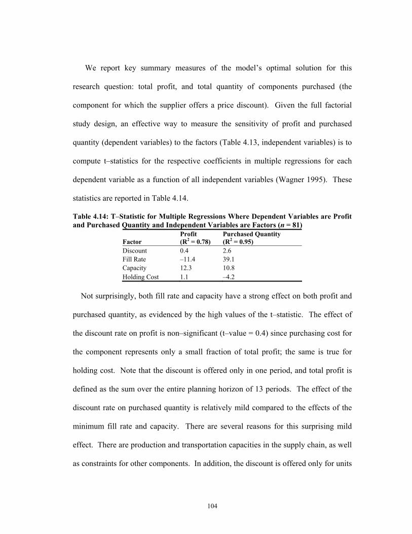
104
We report key summary measures of the model’s optimal solution for this
research question: total profit, and total quantity of components purchased (the
component for which the supplier offers a price discount). Given the full factorial
study design, an effective way to measure the sensitivity of profit and purchased
quantity (dependent variables) to the factors (Table 4.13, independent variables) is to
compute t–statistics for the respective coefficients in multiple regressions for each
dependent variable as a function of all independent variables (Wagner 1995). These
statistics are reported in Table 4.14.
Table 4.14: T–Statistic for Multiple Regressions Where Dependent Variables are Profit and Purchased Quantity and Independent Variables are Factors (n = 81)
Factor Profit (R2 = 0.78)
Purchased Quantity (R2 = 0.95)
Discount 0.4 2.6 Fill Rate –11.4 39.1 Capacity 12.3 10.8 Holding Cost 1.1 –4.2
Not surprisingly, both fill rate and capacity have a strong effect on both profit and
purchased quantity, as evidenced by the high values of the t–statistic. The effect of
the discount rate on profit is non–significant (t–value = 0.4) since purchasing cost for
the component represents only a small fraction of total profit; the same is true for
holding cost. Note that the discount is offered only in one period, and total profit is
defined as the sum over the entire planning horizon of 13 periods. The effect of the
discount rate on purchased quantity is relatively mild compared to the effects of the
minimum fill rate and capacity. There are several reasons for this surprising mild
effect. There are production and transportation capacities in the supply chain, as well
as constraints for other components. In addition, the discount is offered only for units

105
above the minimum purchased quantity specified in the contract with the supplier.
Thus, the discounted components, without a change in the final product’s price, does
not result in a demand increase for the final product, and is therefore mostly used to
increase the fraction of demand that is met with profitable products.
The effect of unit holding cost on profit is also non–significant (Table 4.14); this
occurs because holding costs comprise only a fraction of total profit over the 13–
period planning horizon. The effect of holding cost on the purchased quantity is mild
compared to the effect of the minimum fill rate and the capacity, which is a surprising
result, considering the lot–sizing literature. For example, if the unit holding cost
increases six–fold, the EOQ formula posits that the optimal lot size would decrease
by 60% (= 1 – 1 6 ); our model’s optimal solution recommends instead that the total
quantity of purchased components decreases by an average of only 7.3% (Figure
4.19). Overall, these are interesting results because they point out weaknesses of
simple models in the literature––where assumptions of a single product,
uncapacitated supply chains, and no service level constraints are frequently used––in
dealing with the complexities of global supply chains, where these assumptions do
not hold, and which significantly influence a firm’s optimal sourcing–production–
distribution decision.
Next, we look at the impact of each factor on profit and purchased quantity, by
taking an average across experiments, for each factor level. These are shown in
Figure 4.19 and Figure 4.20 for profit and purchased quantity, respectively. The
relationship between (minimum) fill rate and profit (Figure 4.19) displays the usual

106
shape of profit–service trade–off curves—that is, increasing minimum fill rates
decreases profits at an increasing rate. Also, increasing capacity beyond a certain
level (here, mid level) does not result in significant profit increases (Figure 4.19) or in
additional purchased components (Figure 4.20) and this can be explained as follows.
Additional capacity beyond the low level is used to produce profitable products,
however, additional capacity beyond the middle level would be used to produce non–
profitable products beyond the required service level, which is not economically
attractive and thus does not happen (Figure 4.21); the purchased quantity for non–
profitable products remains unchanged with the capacity level at 267). As discussed
before, holding cost and discount do not significantly affect profits, as evidenced by
the respective “flat” curves.
Figure 4.19: Effect of Holding Cost, Capacity, Fill Rate and Discount on Profit
Profit (averaged across experiments)
2.00E+08
2.05E+08
2.10E+08
2.15E+08
2.20E+08
2.25E+08
2.30E+08
2.35E+08
2.40E+08
LO MID HI
Level of Input
Holding Cost Capacity Fill Rate Discount
Figure 4.20: Effect of Holding Cost, Capacity, Fill Rate, and Discount on the Purchased Quantity

107
Purchased quantity (average across experiments)
30,000
40,000
50,000
60,000
70,000
80,000
90,000
LO MID HI
Level of Input
Holding Cost Capacity Fill Rate Discount
Figure 4.21: Effect of Capacity Increase in the Production of Profitable Products (Average Across Experiments Where Minimum Fill Rate = 0.85)
Purchased Component Quantity for Profitable Products
1450
1500
1550
1600
1650
1700
LO MID HICapacity
4.4.4.2 We now investigate the possibility of passing on part of the component savings to
the customers by offering price discounts for profitable products at sales subsidiaries,
which increases their demand. As demand for profitable products increases, the
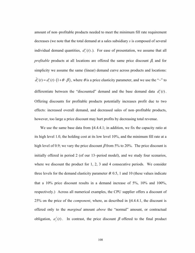
108
amount of non–profitable products needed to meet the minimum fill rate requirement
decreases (we note that the total demand at a sales subsidiary s is composed of several
individual demand quantities, )(td si .). For ease of presentation, we assume that all
profitable products at all locations are offered the same price discount β, and for
simplicity we assume the same (linear) demand curve across products and locations:
( )( ) ( ) 1s si id t d t θ β= ⋅ + ⋅% , where θ is a price elasticity parameter, and we use the “~” to
differentiate between the “discounted” demand and the base demand data ( )sid t .
Offering discounts for profitable products potentially increases profit due to two
effects: increased overall demand, and decreased sales of non–profitable products,
however, too large a price discount may hurt profits by decreasing total revenue.
We use the same base data from §4.4.4.1; in addition, we fix the capacity ratio at
its high level 1.0, the holding cost at its low level 10%, and the minimum fill rate at a
high level of 0.9; we vary the price discount β from 5% to 20%. The price discount is
initially offered in period 2 (of our 13–period model), and we study four scenarios,
where we discount the product for 1, 2, 3 and 4 consecutive periods. We consider
three levels for the demand elasticity parameter θ: 0.5, 1 and 10 (these values indicate
that a 10% price discount results in a demand increase of 5%, 10% and 100%,
respectively.) Across all numerical examples, the CPU supplier offers a discount of
25% on the price of the component, where, as described in §4.4.4.1, the discount is
offered only to the marginal amount above the “normal” amount, or contractual
obligation, ( )fja t . In contrast, the price discount β offered to the final product
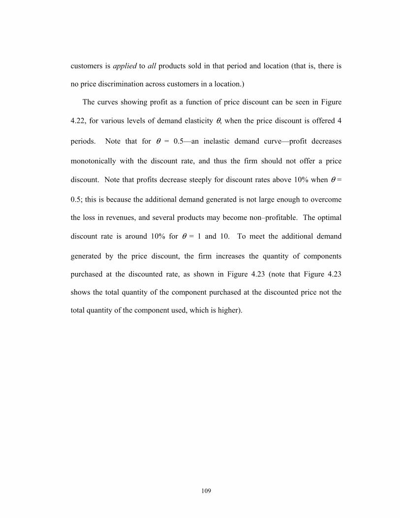
109
customers is applied to all products sold in that period and location (that is, there is
no price discrimination across customers in a location.)
The curves showing profit as a function of price discount can be seen in Figure
4.22, for various levels of demand elasticity θ, when the price discount is offered 4
periods. Note that for θ = 0.5––an inelastic demand curve––profit decreases
monotonically with the discount rate, and thus the firm should not offer a price
discount. Note that profits decrease steeply for discount rates above 10% when θ =
0.5; this is because the additional demand generated is not large enough to overcome
the loss in revenues, and several products may become non–profitable. The optimal
discount rate is around 10% for θ = 1 and 10. To meet the additional demand
generated by the price discount, the firm increases the quantity of components
purchased at the discounted rate, as shown in Figure 4.23 (note that Figure 4.23
shows the total quantity of the component purchased at the discounted price not the
total quantity of the component used, which is higher).
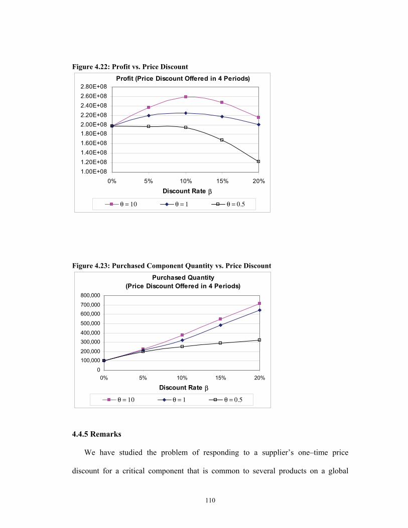
110
Figure 4.22: Profit vs. Price Discount Profit (Price Discount Offered in 4 Periods)
1.00E+081.20E+081.40E+081.60E+081.80E+082.00E+082.20E+082.40E+082.60E+082.80E+08
0% 5% 10% 15% 20%
Discount Rate β
θ = 10 θ = 1 θ = 0.5
Figure 4.23: Purchased Component Quantity vs. Price Discount
Purchased Quantity (Price Discount Offered in 4 Periods)
0
100,000200,000
300,000400,000
500,000
600,000700,000
800,000
0% 5% 10% 15% 20%
Discount Rate β
θ = 10 θ = 1 θ = 0.5
4.4.5 Remarks We have studied the problem of responding to a supplier’s one–time price
discount for a critical component that is common to several products on a global

111
supply chain, using real data from Toshiba Corporation. We use an MIP–type
formulation for a 13–week planning horizon, but for implementation purposes we
simplify it to a linear program. Our model is a tactical planning model; we neither
consider strategic issues such as facility location nor tactical issues such as production
scheduling. Our model’s primary decision variables are flows of materials in the
supply chain along paths (as opposed to flows along single arcs), which isolates
critical information regarding profitable and non–profitable products across
locations—products that are profitable in one location may not be profitable in
another location. This information serves as an input to the more strategic decision of
product line offering. Our model maximizes profit subject to a critical service level
constraint—a minimum fill rate, which may be different across locations. Because of
the minimum fill rate, the firm may need to sell non–profitable products. Thus, our
research studies one of many weapons a firm has to mitigate the effect of non–
profitable products on the firm’s profitability.
Temporary price discounts by suppliers are a relatively common phenomenon.
We consider the issue of coordinating a temporary price discount for a critical
component with pricing and sales at different locations in a global, capacitated,
sourcing–manufacturing–distribution supply chain. Based on data from Toshiba, we
perform a numerical study where we vary critical parameters on the supply chain—
capacity, discount rate, holding cost, number of discounted periods, and minimum fill
rate—and analyze their impact on the firm’s profitability. We find that capacity
critically impact profits, however, adding capacity beyond a certain level, without
changes in the firm’s pricing strategy, only impacts the production of non–profitable
112
products, which does not result in profit improvement if the firm is above the
minimum fill rate threshold. The relationship between minimum fill rate and profit
has the usual shape of a profit–service trade–off curve. We also point out the
weaknesses of analytical models in dealing with the complexities of decision–making
in global supply chains. For example, we show how a six–fold increase in holding
cost for a component only results in a 7% increase in the optimal lot size, whereas the
EOQ model predicts a 60% increase. This occurs because the assumptions of
uncapacitated supply chains—including production and transportation—as well as a
single product type, typical of analytical models, do not hold in complex supply
chains.
We find that passing on temporary component price discounts to final product
customers is attractive if the demand curve is “elastic” enough such that a price
discount significantly stimulates demand. Also, a price discount needs to be offered
for several periods (weeks in this case) for it to be effective and profitable. For
example, it is not optimal to offer price discount on the final product during only one
period under any scenario analyzed in this paper. We find that the relationship
between price discount and the number of periods when the discount is offered is non
monotonic, requiring careful optimization.
Although our study was conducted with real data from a global company, we
caution on some of its limitations. The primary limitation regards modeling the
demand curve. Essentially, we have assumed demands to be independent across
products—discounts offered in one product would not impact demand for other
products. Also, our analysis considers competitive issues only on a limited basis,
113
through the estimated demand curve––for example, we assume that if the firm offers
no discounts on its final product, even after receiving a discount on a critical
component by a key supplier, then its demand does not change. In reality, it is likely
that the supplier offers discounts to several manufacturers; thus the demand curve
should include price dynamics by all other competitive products in the marketplace;
this, however, significantly complicates modeling and parameter estimation for the
demand curves.

114
Chapter 5 Conclusions Global competition and e-commerce have imposed tremendous pressure on
product and service providers to get closer to the customers. At the same time end
consumers are becoming increasingly knowledgeable and demanding. Consequently,
in the current customer-centric business environment, supply chains must be designed
to accommodate for real-time responsiveness, uncertain customer orders, globally
dispersed locations and diminishing profit margin. Therefore, managing supply
chains in today's distributed manufacturing environment has become more complex.
To remain competitive in today's global marketplace, organizations must streamline
their supply chains. The practice of coordinating design, procurement, flow of goods,
services, information and finances, beginning from raw material flows, parts supplier,
manufacturer, distributor, retailer, and finally to consumer requires synchronized
planning and execution. It is of critical importance to understand how an efficient
and effective supply chain is affected by order promising and order fulfillment
strategies. In this dissertation, we study two issues related to moving a company from
an Available to Promise (ATP) philosophy to a Profitable to Promise (PTP)
philosophy: pseudo order promising and coordinating demand fulfillment with
supply.
To address the first issue, a single time period analytical ATP model for n
confirmed customer orders and m pseudo orders is presented by considering both

115
material constraints and production capacity constraints. At the outset, some
analytical properties of the optimal policies are derived and then a particular customer
order promising scheme is derived based on the ratio between customer service level
and profit. Algorithms presented to solve this problem provide decision makers the
effective rule-based mechanism to implement and deploy critical decisions in real-
time ATP systems.
To tackle the second issue, we explore two cases: a deterministic demand curve
or stochastic demand. In the first case, a constrained non-linear programming model
is developed. For the second case a stochastic constrained model is formulated to
determine both the quantity of raw materials to purchase from suppliers and demand
fulfillment levels for each end product in every location. A simple, yet generic
optimal solution structure is derived and a series of numerical studies and sensitivity
analysis are carried out to investigate the impact of different factors on profit and
fulfilled demand quantity. The objective of this analysis is to understand the
implication of factors like price elasticity, path cost, shortage cost and holding cost,
along with their interaction effects within the firm's supply chain. Further, we present
an analytical model to explore balanced supply. Implementation of the resulting
generic rules reduces response time and provides managers with insight into the
optimal policies that improve demand fulfillment and simultaneously reduce risk
through balanced supply.
Further, the firm’s optimal response to a one-time-period discount offered by the
supplier of a key component is studied under two different strategies: a) Not passing
along the discount to its customers b) Offering price discounts to increase the demand

116
for profitable products. Unlike most models of this type in the literature, which define
variables in terms of single arc flow, this model employs path variables to directly
identify and manipulate profitable and non-profitable products. Numerical
experiments based on Toshiba’s global notebook supply chain are conducted. Based
on the results, an interesting relationship among capacity, fill rate and profit is
observed. Furthermore, it is found that passing on temporary component price
discounts to end product customers is attractive if the demand curve is “elastic”
enough so that a price discount significantly stimulates demand.

117
Appendices Appendix 1:
Proof of Theorem 3.1:
It suffices to show that the Hessian matrix of the objective function, Hn+1×n+1, is
negative definite. Let En+1×n+1 be the matrix with each entry of 1. Then we have
H=diag( )qX
(''sq 2
1
121
1β , )qX
(''sq 2
2
222
2β,…, )
qX
(''sq 2
n
n2n
nβ, -(p+h)f(Y))-( )z(''m)z(''g + )E
where z= YXn
1ii +∑
=
.
Let θ=(θ1,…, θn+1)T,
21n
n
1i
2i
21n
1ii
21n
1ii
21n
2i
i
in
1i i
i
T
K)hp(LU)(M
))](z(''m)z(''g[)Y(f)hp()qX
(''sq
H
+=
+
=
+
=+
=
θ+−θ+θ−≤
θ+−θ+−θβ
=
θθ
∑∑
∑∑
If M > 0, RHS ≤ 0 and RHS = 0 only if θ =0. Hence H will be negative definite.
If M ≤ 0, we have,
21n
n
1i
2i
21n
n
1i
2i
1n
1i
2i
T
)]1n(MK)hp[()]1n(MLU[
K)hp(LU)1n(M
H
+=
+=
+
=
θ+++−θ+−=
θ+−θ+θ+−≤
θθ
∑
∑∑
then, by the assumption of the theorem, H is still negative definitive. Q.E.D.
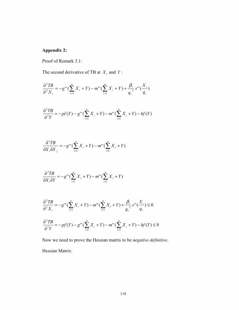
118
Appendix 2:
Proof of Remark 3.1:
The second derivative of TB at iX and Y :
)()('')('')(11
2
2
YhfYXmYXgYpfY
TB n
ii
n
ii −+−+−−=
∂∂ ∑∑
==
)('')(''11
2
YXmYXgXX
TB n
ii
n
ii
ji
+−+−=∂∂
∂ ∑∑==
)('')(''11
2
YXmYXgYX
TB n
ii
n
ii
i
+−+−=∂∂
∂ ∑∑==
0)('')('')('' 211
2
2
≤++−+−=∂∂ ∑∑
== i
i
i
in
ii
n
ii
i qX
sq
YXmYXgXTB β
0)()('')('')(11
2
2
≤−+−+−−=∂
∂ ∑∑==
YhfYXmYXgYpfY
TB n
ii
n
ii
Now we need to prove the Hessian matrix to be negative definitive.
Hessian Matrix:
)('')('')('' 211
2
2
i
i
i
in
ii
n
ii
i qX
sq
YXmYXgXTB β
++−+−=∂∂ ∑∑
==

119
⎟⎟⎟⎟⎟⎟⎟⎟⎟⎟⎟
⎠
⎞
⎜⎜⎜⎜⎜⎜⎜⎜⎜⎜⎜
⎝
⎛
∂∂
∂∂∂
∂∂∂
∂∂∂
∂∂∂
∂∂∂
∂∂∂
∂∂∂
∂∂∂
∂∂∂
∂∂
∂∂∂
∂∂∂
∂∂∂
∂∂∂
∂∂
YTB
XYTB
XYTB
XYTB
YXTB
XXTB
XXTB
XXTB
YXTB
XXTB
XTB
XXTB
YXTB
XXTB
XXTB
XTB
n
nnnnn
n
n
2
22
2
2
1
2
22
2
2
1
2
2
2
2
2
22
2
12
21
2
1
2
21
2
12
2
.
.
.....
..
..
= )1()1( +×+ nnHM
For simplicity, let )()(1
YXggn
ii +=⋅ ∑
=
, and )()(1
YXmmn
ii +=⋅ ∑
=
We can decompose the )1()1( +×+ nnHM to be:
)1()1( +×+ nnHM = 321 HHH ++
where :
⎟⎟⎟⎟⎟⎟⎟⎟⎟
⎠
⎞
⎜⎜⎜⎜⎜⎜⎜⎜⎜
⎝
⎛
+−
=
)()(.000
.)(''.00
.....
0.0)(''0
0.00)(''
22
22
222
2
21
121
1
1
YfhpqX
sq
qX
sq
qXs
q
H
n
n
n
nβ
β
β
,which is a
semi-negative definitive.
Q 0()''()'' >+ mg
( )IgH )(''2 ⋅−=
( )ImH )(''3 ⋅−= ,
∴ ))](('')(''[32 ImgHH ⋅+⋅−=+ , which is a negative definitive.
)1()1( +×+ nnHM = 321 HHH ++ ,
∴ )1()1( +×+ nnHM is negative definitive. Q.E.D.

120
Appendix 3:
Proof of Theorem 3.2:
i) Let the sequences { )1('sq
ri
ii
β+ } and { )0('s
qr
i
ii
β+ } be non-decreasingly ordered.
By 0)]1(')][0('[ ≥−− sZsZ ijij , we can prove for any i, j
)1(')1(' sq
rsq
rj
jj
i
ii
ββ+<+ )0('s
qr)0('s
qr
j
jj
i
ii
β+≤
β+ and
)1('sq
r)1('sq
rj
jj
i
ii
β+>
β+ )0('s
qr)0('s
qr
j
jj
i
ii
β+≥
β+
Then, if necessary, we can adjust the order of elements in the above two sequences
to make sure we have simultaneously for any i,
)1('sq
r)1('sq
r1i
1i1i
i
ii
+
++
β+≤
β+ and )0('s
qr)0('s
qr
1i
1i1i
i
ii
+
++
β+≤
β+
ii) For simplicity, let )YX('m)YX('gf *n
1i
*i
*n
1i
*i
* +++= ∑∑==
.
Then there exist unique k and k’ such that
)1('sq
rf)1('sq
r1k
1k1k
*
k
kk
+
++
β+<≤
β+ and )0('s
qrf)0('s
qr
1'k
1'k1'k
*
'k
'k'k
+
++
β+≤<
β+
By s’(0)>s’(1)>0, it is trivial to prove k ≥ k’
iii)
For all 1+≥ ki : 0)()( ' >−=+⋅− iii
i
ii q
Xs
qfr μλβ ,
i.e.: 0>iλ , from 0)( =− iii Xqλ , we have: ,ii qX = ( 1+≥ ki )

121
For all 'ki ≤ : 0)0()()()( '' <+⋅−<+⋅− sq
frqX
sq
fri
ii
i
i
i
ii
ββ
∴ 0)()( ' <+⋅−=−i
i
iiii q
Xs
qfr βμλ ,
i.e. 0>iμ , from: 0=× iXμ , we have: ,0=iX ( 'ki ≤ ).
Q.E.D.

122
Appendix 4:
Proof of Remark 3.2.
Let {Xi*} and Y* be an arbitrary solution to (3.24)-(3.25).
From 1i1i
1ii
i
i r)1('sq
r)0('sq +
+
+ +β
<+β , we can have:
)0(')1('....)0(')1(')0(')1('2
22
2
22
1
11
1
11 s
qrs
qrs
qrs
qrs
qrs
qr
n
nn
n
nn
ββββββ+<+<<+<+<+<+
For simplicity, let )(')(')(1
*
1
* YXmYXgfn
ii
n
ii +++=⋅ ∑∑
==
Without the loss of the generality, there are two cases:
(A): if )1(')()0('1
11 s
qrfs
qr
k
kk
k
kk
+
++ +≤⋅≤+
ββ
then: 1)for :1+≥ ki 0)()( ' >−=+⋅− iii
i
ii q
Xs
qfr μλβ ,
i.e.: 0>iλ , from 0)( =− iii Xqλ , we have: ,ii qX = ( 1+≥ ki )
2) For all :ki ≤
0)0()()()( '' <+⋅−<+⋅− sq
frqX
sq
fri
ii
i
i
i
ii
ββ
∴ 0)()( ' <+⋅−=−i
i
iiii q
Xs
qfr βμλ ,
i.e. 0>iμ , from: 0=× iXμ , we have: ,0=iX ( ki < )
(B) if: )0('sq
r)('m)('g)1('sq
rk
kk
k
kk
β+<⋅+⋅<
β+
then: 1) for :1+≥ ki 0)()( ' >−=+⋅− iii
i
ii q
Xs
qfr μλβ ,
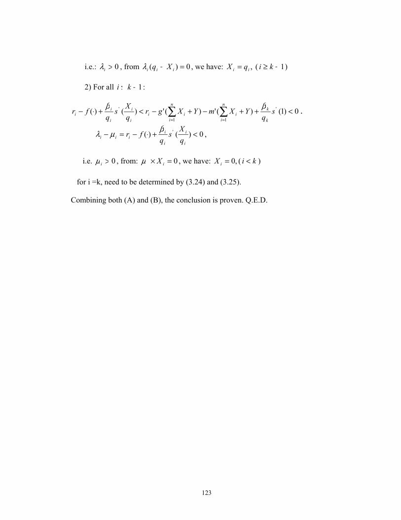
123
i.e.: 0>iλ , from 0)( =− iii Xqλ , we have: ,ii qX = ( 1+≥ ki )
2) For all :1−≤ ki
0)1()(')(')()( '
11
' <++−+−<+⋅− ∑∑==
sq
YXmYXgrqX
sq
frk
kn
ii
n
iii
i
i
i
ii
ββ∴
0)()( ' <+⋅−=−i
i
i
iiii q
Xs
qfr
βμλ ,
i.e. 0>iμ , from: 0=× iXμ , we have: ,0=iX ( ki < )
for i =k, need to be determined by (3.24) and (3.25).
Combining both (A) and (B), the conclusion is proven. Q.E.D.

124
Appendix 5:
Proof of Corollary 3.5.1.
After separating the confirmed orders and pseudo orders, the profit function of
pseudo orders is:
PP =∑∈Jj
jj uYEp ),min( )0,max(∑∈
−−Jj
jj uYEh
Its first order derivative would be:
PP’ = ))()(1((∑∈
−−Jj
jjjj YFhYFp
PP’ = 0))()(( ≥+−∑∈Jj
jjjj YFhpp
And its second order derivative is:
PP’’ = ))()((∑∈
−−Jj
jjjj YfhYfp , which is:
PP’’ = 0))()( ≤+−∑∈Jj
jjj Yfhp
So we can see, the first order of that function is greater than or equal to 0; and its
second order is smaller than or equal to 0; thus the Profit function of Pseudo orders is
concave in terms of order quantity. Q. E. D.
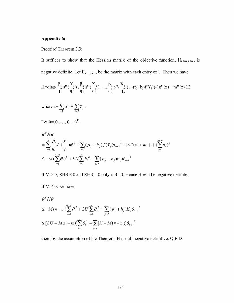
125
Appendix 6:
Proof of Theorem 3.3:
It suffices to show that the Hessian matrix of the objective function, Hn+m×n+m, is
negative definite. Let En+m×n+m be the matrix with each entry of 1. Then we have
H=diag( )qX
(''sq 2
1
121
1β , )qX
(''sq 2
2
222
2β ,…, )qX
(''sq 2
n
n2n
nβ , -(pj+hj)f(Yj))-( )z(''m)z(''g + )E
where z= ∑∑∈=
+Jj
j
n
ii YX
1.
Let θ=(θ1,…, θn+m)T,
2
1
22
1
2
1
22
1
)()(
))](('')(''[)()()(''
jnjJj
jj
n
ii
mn
ii
mn
iijn
Jjjjji
i
in
i i
i
T
KhpLUM
zmzgYfhpqX
sq
H
+∈=
+
=
+
=+
∈=
∑∑∑
∑∑∑
+−+−≤
+−+−=
θθθ
θθθβθθ
If M > 0, RHS ≤ 0 and RHS = 0 only if θ =0. Hence H will be negative definite.
If M ≤ 0, we have,
2
1
2
2
1
2
1
2
)]([)]([
)()(
jnJj
n
ii
jnjJj
jj
n
ii
mn
ii
T
mnMKmnMLU
KhpLUmnM
H
+∈=
+∈=
+
=
++−+−≤
+−++−≤
∑∑
∑∑∑
θθ
θθθ
θθ
then, by the assumption of the Theorem, H is still negative definitive. Q.E.D.

126
Appendix 7:
Proof of Theorem 3.4: We first prove part i)
Let the sequences { )1('sq
ri
ii
β+ } and { )0('s
qr
i
ii
β+ } be non-decreasingly ordered.
By 0)]1(')][0('[ ≥++ sZsZ ijijijij αα , we can prove for any i, j
)1(')1(' sq
rsq
rj
jj
i
ii
ββ+<+ )0('s
qr)0('s
qr
j
jj
i
ii
β+≤
β+ and
)1('sq
r)1('sq
rj
jj
i
ii
β+>
β+ )0('s
qr)0('s
qr
j
jj
i
ii
β+≥
β+
Then, if necessary, we can adjust the order of elements in the above two sequences to
make sure we have simultaneously for any i,
)1('sq
r)1('sq
r1i
1i1i
i
ii
+
++
β+≤
β+ and )0('s
qr)0('s
qr
1i
1i1i
i
ii
+
++
β+≤
β+
For simplicity, let )(')('1
*
1
*
1
*
1
** ∑∑∑∑====
+++=m
jj
n
ii
m
jj
n
ii YXmYXgf .
Then there exist unique k and k’ such that
)1(')1('1
11
* sq
rfsq
rk
kk
k
kk
+
++ +<≤+
ββ and )0('s
qrf)0('s
qr
1'k
1'k1'k
*
'k
'k'k
+
++
β+≤<
β+
By s’(0)>s’(1)>0, it is trivial to prove k ≥ k’
For all 1+≥ ki : 0)('* >−=+− iii
i
ii q
Xs
qfr μλβ ,
i.e.: 0>iλ , from 0)( =− iii Xqλ , we have: ,ii qX = ( 1+≥ ki )
For all 'ki ≤ : 0)0()( '*'* <+−<+− sq
frqX
sq
fri
ii
i
i
i
ii
ββ

127
∴ 0)('* <+−=−i
i
iiii q
Xs
qfr βμλ ,
i.e. 0>iμ , from: 0=× iXμ , we have: ,0=iX ( 'ki ≤ ).
Now we will show ii)
From (3-47), we have jj
jjj hp
fwpYF
+−+
=*
)( , where wj>=0. Obviously when
*fp j < , wj has to be positive which then implies Yj=0 by (3-47). On the other hand,
if *fp j < , we have Yj>0 and solves equation (3-50). Apply similar arguments to the
case where *fp j = , we still get Yj=0. We complete part (ii) by rephrasing our
arguments above.
Q.E.D.
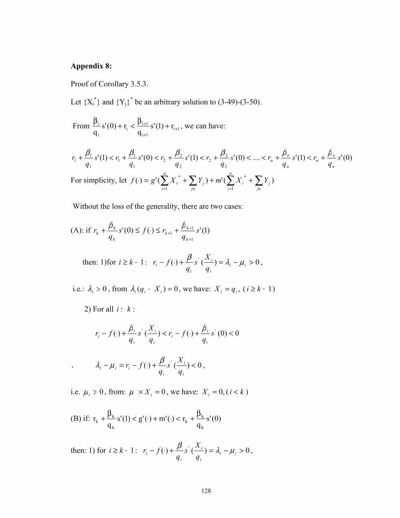
128
Appendix 8:
Proof of Corollary 3.5.3.
Let {Xi*} and {Yj}* be an arbitrary solution to (3-49)-(3-50).
From 1i1i
1ii
i
i r)1('sq
r)0('sq +
+
+ +β
<+β , we can have:
)0(')1('....)0(')1(')0(')1('2
22
2
22
1
11
1
11 s
qrs
qrs
qrs
qrs
qrs
qr
n
nn
n
nn
ββββββ+<+<<+<+<+<+
For simplicity, let )(')(')(1
*
1
* ∑∑∑∑∈=∈=
+++=⋅j
j
n
ii
jj
n
ii YXmYXgf
Without the loss of the generality, there are two cases:
(A): if )1(')()0('1
11 s
qrfs
qr
k
kk
k
kk
+
++ +≤⋅≤+
ββ
then: 1)for :1+≥ ki 0)()( ' >−=+⋅− iii
i
ii q
Xs
qfr μλβ ,
i.e.: 0>iλ , from 0)( =− iii Xqλ , we have: ,ii qX = ( 1+≥ ki )
2) For all :ki ≤
0)0()()()( '' <+⋅−<+⋅− sq
frqX
sq
fri
ii
i
i
i
ii
ββ
∴ 0)()( ' <+⋅−=−i
i
iiii q
Xs
qfr βμλ ,
i.e. 0>iμ , from: 0=× iXμ , we have: ,0=iX ( ki < )
(B) if: )0('sq
r)('m)('g)1('sq
rk
kk
k
kk
β+<⋅+⋅<
β+
then: 1) for :1+≥ ki 0)()( ' >−=+⋅− iii
i
ii q
Xs
qfr μλβ ,

129
i.e.: 0>iλ , from 0)( =− iii Xqλ , we have: ,ii qX = ( 1+≥ ki )
2) For all :1−≤ ki
0)1()(')(')()( '
1
*
1
*' <++−+−<+⋅− ∑∑∑∑∈=∈=
sq
YXmYXgrqX
sq
frk
k
jj
n
ii
jj
n
iii
i
i
i
ii
ββ∴
0)()( ' <+⋅−=−i
i
i
iiii q
Xs
qfr
βμλ ,
i.e. 0>iμ , from: 0=× iXμ , we have: ,0=iX ( ki < )
for i =k, need to be determined by (3-49) and (3-50).
Combining both (A) and (B), the first part is proven.
Now we know that ∑∈
≥Ii
i qX * From part ii) of Theorem 3.4, Yj>0 only if
)(')(' ∑∑∑∑∈∈∈∈
+++>Jj
jIi
iJj
jIi
ij YXmYXgp
Since 0)('')('' >+++ ∑∑∑∑∈∈∈∈ Jj
jIi
iJj
jIi
i YXmYXg , we know
)(')(' ∑∑∑∑∈∈∈∈
+++Jj
jIi
iJj
jIi
i YXmYXg is increasing.
Thus we have
*)('*)(')(')(' qmqgYXmYXgpJj
jIi
iJj
jIi
ij +>+++> ∑∑∑∑∈∈∈∈
when Yj > 0. This is equivalent to the second part of the corollary.
Q.E.D.
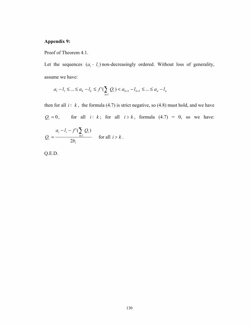
130
Appendix 9:
Proof of Theorem 4.1.
Let the sequences )( ii la − non-decreasingly ordered. Without loss of generality,
assume we have:
nnkkIi
ikk lalaQflala −≤≤−<≤−≤≤− ++∈∑ ...)('... 1111
then for all ki ≤ , the formula (4.7) is strict negative, so (4.8) must hold, and we have
0=iQ , for all ki ≤ ; for all ki > , formula (4.7) = 0, so we have:
i
Iiiii
i b
QflaQ
2
)(' ∑∈
−−= for all ki > .
Q.E.D.
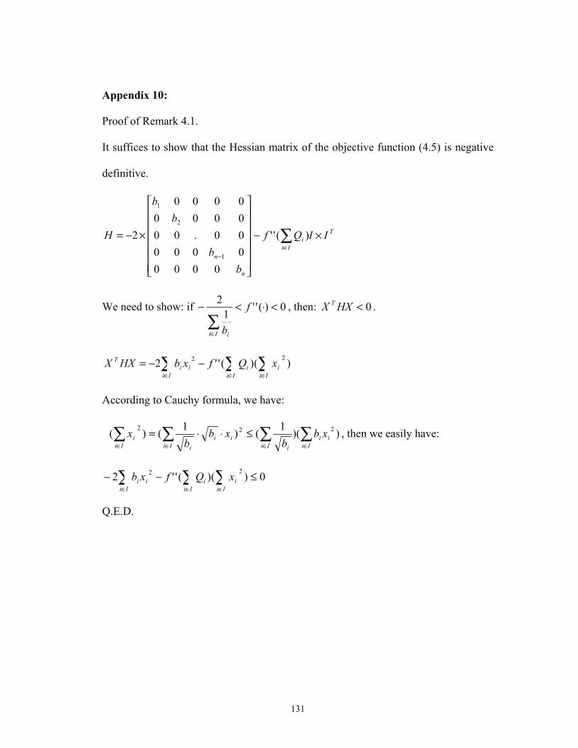
131
Appendix 10:
Proof of Remark 4.1.
It suffices to show that the Hessian matrix of the objective function (4.5) is negative
definitive.
T
Iii
n
n
IIQf
bb
bb
H ×−
⎥⎥⎥⎥⎥⎥
⎦
⎤
⎢⎢⎢⎢⎢⎢
⎣
⎡
×−= ∑∈
−
)(''
0000000000.0000000000
2
1
2
1
We need to show: if 0)(''1
2 <⋅<−∑∈
f
bIi i
, then: 0<HXX T .
)()(''2 22 ∑∑∑∈∈∈
−−=Ii
iIi
iiIi
iT xQfxbHXX
According to Cauchy formula, we have:
))(1()1()( 222i
Iii
Ii iii
Ii iIii xb
bxb
bx ∑∑∑∑
∈∈∈∈
≤⋅⋅= , then we easily have:
0)()(''2 22 ≤−− ∑∑∑∈∈∈ Ii
iIi
iiIi
i xQfxb
Q.E.D.

132
Appendix 11:
Proof of Remark 4.1
0)()()0(0
0
=−= ∫ iiiii duufuSW
0)0()0(' == FWi
and: Q )()(' iii SFSW =
∴ 0)()(" >= iii SfSW
So the )(⋅iW is a convex function.
Q.E.D.

133
Appendix 12 :
Proof of Theorem 4.2.
Let the sequences )( iii ldp −+ non-decreasingly ordered. Without loss of generality,
assume we have:
nnnkkkIi
ikkk ldpldpSgldpldp −+≤≤−+<≤−+≤≤−+ +++∈∑ ...)('... 111111
then for all ki ≤ , the formula (4.12) is strict positive; to let (4.13) hold, we have
0=iS for all ki ≤ ;
On the other hand, for all ki > , when nnnkkkIi
i ldpldpSg −+≤≤−+< +++∈∑ ...)(' 111 ,
we have: 0)(' >ii SW . We also know: )(⋅iW is convex and 0)0(' =iW ,
∴ 0>iS .
Q 0>iS and 0=ii Sλ
∴ 0)()()()( '' =−+−+++= ∑ iiii
iiiiiii ldpSgSWhdpλ
so we have: iii
Iiiiii
iii hdp
SgldpSFSW
++
−−+==
∑∈
)(')()()(' for all ki > .
Q.E.D.

134
Appendix 13.
Q )(⋅iW is convex function, ∴ )(' ⋅iW is a increasing function which goes from 0
when iS =0 to 1 when iS = infinity
Q 0)0(' =iW , and
1)(
)(' <++−+
<iii
iiiii hdp
ldpSW
∴ iS has upper bound.
∴ ∑=i
iSQ has upper bound.
Q.E.D.

135
Appendix 14:
Proof of Remark 4.2.
It suffices to show that the Hessian matrix of the objective function
ii
S
i iiiiiiii
iiii SldpSgduufuSdhp
i
)()()()()(0
−+−+−++ ∫ ∑ ∑∑
is positive definitive. We have:
T
Iii
nnnn
nnnn
IISg
SfdhpSfdhp
SfdhpSfdhp
H
×+
⎥⎥⎥⎥⎥⎥
⎦
⎤
⎢⎢⎢⎢⎢⎢
⎣
⎡
++++
++++
=
∑∈
−−−−
)(''
)()(00000)()(00000.00000)()(00000)()(
1111
2222
1111
Now we need to show: if UGUFdhpi iii
×>++∑ )(
1 , then: 0>HXX T ; where UF
and UG is the upper bound of )(⋅f and )('' ⋅− g respectively.
)()('')()( 22 ∑∑∑∈∈∈
+++=Ii
iIi
iiIi
iiiiT xSgxSfdhpHXX
According to Cauchy formula, we have:
))()()(
)()(1(
))()()()(
1()(
2
22
∑∑
∑∑
∈∈
∈∈
++++
≤
⋅++⋅++
=
Iiiiiii
Ii iiii
iiiiiIi iiiiIi
i
xSfdhpSfdhp
xSfdhpSfdhp
x
,
then we easily have:
)()('')()( 22 ∑∑∑∈∈∈
−>++Ii
iIi
iiIi
iiii xSgxSfdhp
∴ 0)()('')()( 22 >+++ ∑∑∑∈∈∈ Ii
iIi
iiIi
iiii xSgxSfdhp Q.E.D.

136
Appendix 15:
Proof of Remark 4.3.
Proof: If there exists optimal solution for problem (4.9)-(4.10), then Hessian Matrix
of the objective function
∑ ∑∑ ∫ −+−+−++i i
iiiiii
S
iiii SldpSgduufuSdhpi
)()()()()(0
is positive definite, and its Hessian matrix can be written as:
⎟⎟⎟⎟⎟⎟
⎠
⎞
⎜⎜⎜⎜⎜⎜
⎝
⎛
++
++++
=
)()(.000...00.....0.0)()(00.00)()(
2222
1111
nnnn Sfdhp
SfdhpSfdhp
H +
∑i
iSg )(''
⎟⎟⎟⎟⎟⎟
⎠
⎞
⎜⎜⎜⎜⎜⎜
⎝
⎛
1.111.1..11.....1.1111.111
H being positive definite means, for any 0),...,( 21 ≠= nXXXX , 0>TXHX .
We have:
∑ ∑ ∑+++=i i i
iiiiiiiT XSgXSfdhpXHX 22 ))(('')()(
Using Cauchy inequality, we have:

137
∑ ∑ ∑≥++++i i i
iiiiiiiiii
XXSfdhpSfdhp
22 )())()()()()(
1(
So:
∑∑∑
+
++
≥i
ii
i
i iiii
T XSg
Sfdhp
XHX 2)())(''
)()(1
1(
And Positive Definite implies:
∑∑
>+
++i
i
i iiii
Sg
Sfdhp
0)(''
)()(1
1
In Theorem 4.2, we have optimal solution:
0=iS for all ki ≤ ,
(4.12)
iii
Iiiiii
i hdp
SgldpSF
++
−−+=
∑∈
)(')()( for all ki > .
(4.13)
So from (4.13), we have:
))('
1(1
iii
Iiiii
i hdp
SglhFS
++
++−=
∑∈−

138
∑ ∑∈
−
++++
−==i Ki iii
iii hdp
QglhFSQ
*
1 ))('
1(
*K is the set of i such that (4.13) holds.
Without loss of generality, we assume 1 *K∈ , Now we look at 1p
Q∂∂ :
Define function )(QR as: QhdpQglh
FQRiii
ii
Ki
−++
++−= ∑
∈
− ))('
1()(*
1
QRpR
pQ
∂∂∂∂
−=∂∂ 1
1
, and let’s look as signs of 1p
R∂∂ and
QR
∂∂ :
0)
)('1((
)()('
1
2111
11
1
≥
++++
−
++++
=∂∂
−
iii
ii
hdpQglh
Ff
hdpQglh
pR
∑∈ −
−
++++
−
++−
=∂∂
*
1)
)('1((
)(''
1Ki
iii
ii
iii
hdpQglh
Ff
hdpQg
QR
= ∑∈
−++
−*
1))((
)(''
Ki iiii hdpSfQg ,
∑≤≤
−++
−≤ni iiii hdpSf
Qg1
1))((
)(''
0<
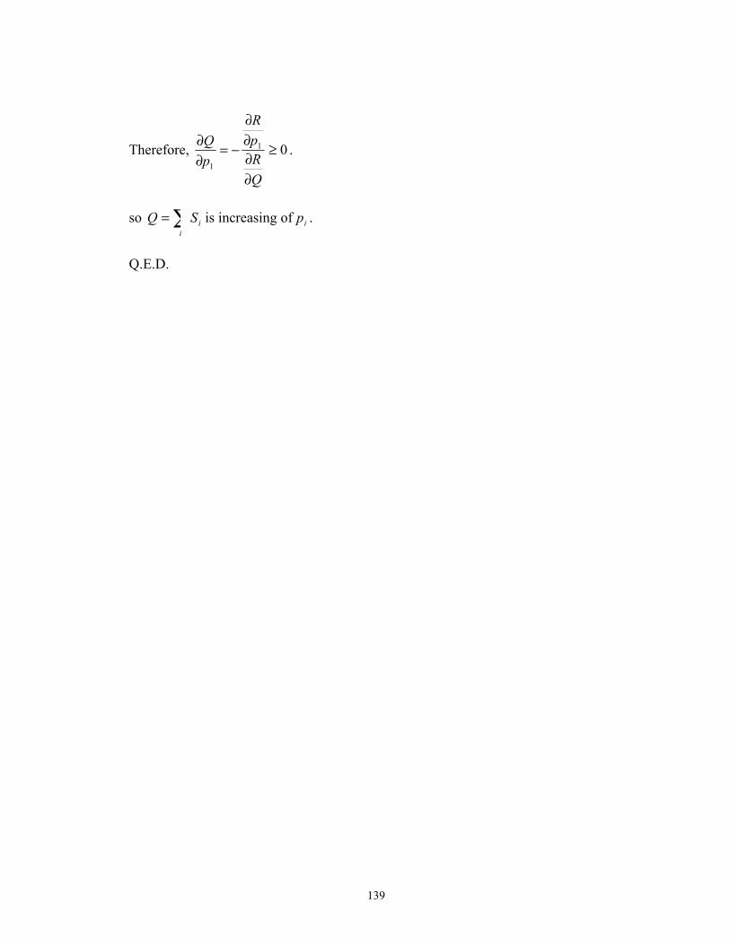
139
Therefore, 01
1
≥
∂∂∂∂
−=∂∂
QRpR
pQ .
so ∑=i
iSQ is increasing of ip .
Q.E.D.

140
Appendix 16.
Proof of Theorem 4.3.
Proof: suppose the optimal solution is ),....,( 21 nxxx , where 01 =x . We will construct
a new solution ( )',....',' 21 nxxx . If we can show this new solution is better than the old
one, we complete our proof by contraposition. The construction of new solution is as
follows:
For ni ≤≤2 ,
we have: 0'=ix if 0=ix ; ii lx =' if ii lx ≥ ,
For 1=i ,
we have: ∑≤<
−=ni
ixQx1
1 '' .
Since we assume ∑>i
ilQ , it is trivial to show that 11 ' lx ≥ .
Now we compare the objective value of the two solutions. Let z and 'z as the
objective values associated with old solution and new solution respectively. We only
need to show that: zz <' .
We have: 1))'()'()((' BxxCxfxfzz iiiiii
+−+−=− ∑ , (note the reason we have
time 1B is because 01 =x and 11 ' lx ≥ )
We denote 'iii xx −=δ , and we have:
∑ =i
i 0δ ,
01 <δ , )
0≥iδ for ni ≤≤1
141
Applying Mean-Value Theorem to the term )'()( ii xfxf − yields:
1)(' BCzzi
iiii ++=− ∑ δδξ
where i
iii
xfxfδ
ξ )'()( −= and )0(')('0 fQf i ≤≤< ξ .
Plugging ∑ =i
i 0δ into the above formula, we have:
111 1
2111 ))0(')('()(' BfQfCCBCCzz ini ni
iii +−+−≥+−+−=− ∑ ∑≤< ≤<
δδξξ 01 >≥ B
Q.E.D.

142
Appendix 17
Proof of Theorem 4.4.
suppose some ix , say 22 lx > , we will construct a new solution which turns out to be
better than the old one. Now we know 11 lx ≥ from Theorem 1. To construct a new
solution, we keep all ix except 1x and 2x unchanged in the new solution.
However, 22 ' lx = , and 2211 ' lxxx −+= .
It is trivial to show the new solution is feasible. So we have:
22112121 )'()'()()(' δδ CCxfxfxfxfzz ++−−+=−
where 120 δδ −=< , still applying Mean-Value Theorem, we have:
0)(' 21212 >−+−=− δξξCCzz
Q.E.D.
143
BIBLIOGRAPHY
[1] Agrawal, V. and Seshadri, S, 1999, “Impact of Uncertainty and Risk Aversion on
Price and Order Quantity in the Newsvendor Problem”, Manufacturing &
Service Operations Management, 2, 410-423.
[2] Ardalan A., 1995, "A Comparative Analysis of Approaches for Determining
Optimal Price and Order Quantity When a Sale Increases Demand", European
Journal of Operational Research, 84, 416–430.
[3] Balakrishnan, A. and J. Geunes, 2000, "Requirements Planning with
Substitutions: Exploring Bill–of–Materials Flexibility in Production Planning",
Manufacturing & Service Operations Management, 2, 166–185.
[4] Ball, M. O., S. Boyson, C.–Y. Chen, E. Rabinovich, L. Raschid, V. Sambamurthy
and V. Zadorozhny, 2001, "Scalable Supply Chain Infrastructures and Their
Impact on Organizations", Proceedings of the 2001 NSF Design and
Manufacturing Research, Tampa.
[5] Ball, M. O., S. Boyson, L. Raschid and V. Sambamurthy, 2000, "Scalable Supply
Chain Infrastructures: Models and Analysis", Proceedings of the 2000 NSF Design
& Manufacturing Research Conference, Vancouver.
[6] Ball, M.O., Chen, C-Y. and Zhao, Z., 2003, “Material Compatibility Constraints
for Make-To-Order Production Planning”, Operations Research Letters , 31 , 420-
428.

144
[7] Bassok, Y. and R. Anupindi, 1997, "Analysis of Supply Contracts With Total
Minimum Commitment", IIE Transactions, 29, 373–381.
[8] Baumol, W.J. and Wolf, P, 1958, “A Warehouse Location Problem”, Operations
Research, 6, 252-8.
[9] Belobaba, Peter, 1987, "Airline Yield Management: An Overview of Seat
Inventory Control", Transportation Science, 21, 63-73.
[10] Belobaba, Peter,1989, ``Application of a Probabilistic Decision Model to
Airline Seat Inventory Control''. Operations Research, 37, 183-197.
[11] Bhattacharjee, S. and R. Ramesh, 2000, "A Multi–Period Profit Maximizing
Model for Retail Supply Chain Management: An Integration of Demand and
Supply–Side Mechanisms", European Journal of Operational Research, 122,
584–601.
[12] Bitran, G. and S. Mondschein, 1995, "An Application of Yield Management to
the Hotel Industry Considering Multiple Day Stays", Operations Research, 43,
427- 448.
[13] Bitran, G., R. Caldentey, S. Mondschein, 1998, "Coordinating
Clearance
Markdown Sales of Seasonal Products in Retail Chains", Operations
Research,
46, 609---624.
[14] Blanchini, Franco, Stefano Miani and Franca Rinaldi, 2004, “Guaranteed Cost
Control for Multi-inventory Systems with Uncertain Demand”, Automatica,

145
40, 213-223
[15] Cattani, K, 1998, “Demand Pooling Effects of a Universal Product when
Demand is from Distinct Markets”, European Journal of Operations
Research, 135, 582-601.
[16] Cattani, K. and G. C. Souza (2002), "Inventory Rationing and Shipment
Flexibility Alternatives for Direct Market Firms," Production and Operations
Management, 11, 4.
[17] Chen, C-Y. , Zhao, Z. and Ball, M.O., 2002, “A Model for Batch Available-to-
Promise”, Production and Operations Management, 11, 424 - 440
[18] Chen, C-Y. , Zhao, Z. and Ball, M.O, 2001, “Quantity and Due Date Promising
Available to Promise”, Information Systems Frontiers, 3 , 477-488.
[19] Chen, F., A. Federgruen and Y.–S. Zheng, 2001, "Near–Optimal Pricing and
Replenishment Strategies for a Retail/Distribution System," Operations
Research, 49, 839–853.
[20] Chen, F. Y. and D. Krass, 2001, "Analysis of Supply Contracts with Minimum
Total Order Quantity Commitments and Non–Stationary Demands," European
Journal of Operational Research, 131, 302–233.
[21] Chen, F., 2001, "Market Segmentation, Advanced Demand Information, and
Supply Chain Performance," Manufacturing & Service Operations Management,
3, 53–67.
[22] Cheng, F. and M.Ettl, 2002, “Inventory-service Optimization in Configure-To-
Order Systems”, Manufacturing & Service Operations Management, 4, 114-
126

146
[23] Cohen, M. and H. L. Lee, 1989, "Resource Deployment Analysis of Global
Manufacturing and Distribution Networks," Journal of Manufacturing and
Operations Management, 2, 81–104.
[24] Cplex, 1998, "Using The Cplex Callable Library", Version 6.0. Incline Village,
NV, ILOG, Inc.
[25] Das, S. and L.Abdel-Malek, 2005, “Modeling the flexibility of order quantities
and lead-times in supply chains”, International Journal of Production
Economics, 85, 171-181
[26] Deshpande, V., M. Cohen and K. Donohue, 2003, "A Threshold Inventory
Rationing Policy for Service Differentiated Demand Classes," Management
Science, 49, 683-703
[27] eB2x, I., 2000, "Why Promising Orders? How Strategic Order Promising Helps
Supply Chains Compete in the New Economy," Online, http://www.eb2x.com.
[28] Federgruen, A. and A. Heching, 1999, "Combined Pricing and Inventory
Control under Uncertainty," Operations Research, 47, 454–475.
[29] Feldman, E., Lehrer, F.A. and Ray, T.L., 1966, “Warehouse Location Under
Continuous Economies of Scale”, Management Science, 12, 670-84.
[30] Feng, Y., G. Gallego., 2000, "Perishable Asset Revenue Management
with
Markovian Time Dependent Demand Intensities", Management
Science, 46,
941---956.
147
[31] Fordyce, K. and G. Sullivan, 1999, "Supply Chain Management, Decision
Technology, and E–Business Information Technology at IBM Microelectronics,"
MicroNews (http://chips.ibm.com/micronews), 5, 4.
[32] Galeotti, Marzio and Louis J. Maccini, Fabio Schiantarelli, 2005, “Inventories,
Employment and Hours”, Journal of Monetary Economics,138, 72-85
[33] Gallego, G., G. van Ryzin, 1997, "A Multi-product, Multi-resource
Pricing
Problem and Its Applications to Network Yield Management",
Operations
Research, 45, 24---41.
[34] Ghali, M., 2003, "Production-planning Horizon, Production Smoothing, and
Convexity of the Cost Functions", International Journal of Production Economics,
81, 67 –74.
[35] Godfrey, G. and Powell, W., 2002, "An Adaptive, Approximate Method for
Stochastic Dynamic Programs with Applications to Inventory and Distribution
Problems", Transportation Science 36, 21-39.
[36] Goetschalckx, M., C. J. Vidal and K. Dogan, 2002, "Modeling and Design of
Global Logistics Systems: A Review of Integrated Strategic and Tactical Model
and Design Algorithms," European Journal of Operational Research, 143, 1–18.
[37] Goh, M. and M. Sharafali, 2002, "Price–Dependent Inventory Models with
Discount Offers Random Times", Production and Operations Management, 11,
139–156.
148
[38] Grant, Hank and Scott Moses, Dave Goldsman, 2002, "Using Simulation to
Adjust Buffer In Order Promising’’, Proceedings of the 2002 Winter
Simulation
Conference
[39] Ha, A., 1997, "Inventory Rationing in a Make–to–Stock Production System with
Several Demand Classes and Lost Sales", Management Science, 43, 1093–1103.
[40] Hall, George, 2002, "Non-Convex Costs and Capital Utilization: A Study of
Production Scheduling at Automobile Assembly Plants", Journal of Monetary
Economics, 47, 113-128.
[41] Horst, R., Tuy, H., 1993, Global Optimization, second edition. Springer, Berlin.
[42] Huchzermeier, A. and M. Cohen, 1996, "Valuing Operational Flexibility under
Exchange Rate Risk", Operations Research, 44, 100–113.
[43] Hunter, Lisa M., 2004, “A Classification of Business-to-Business Buying
Decisions: Risk Importance and Probability as a Framework for e-business
Benefits”, Industrial Marketing Management, 33,145-154.
[44] Johnson, L. and D. Montgomery, 1974, Operations Research in Production
Planning, Scheduling and Control, New York, NY, John Wiley & Sons, Inc.
[45] Kaplan, A., 1969, "Stock Rationing", Management Science, 5, 260–267.
[46] Kelle, P. and E. Silver, 1990, "Safety Stock Reduction by Order Splitting",
Naval Research Logistics, 37, 725–743.
[47] Khouja, Moutaz J., 2000, “Optimal Ordering, Discounting, and Pricing in the
Single-period Problem”, International Journal of Production Economics, 65,
201-216

149
[48] Kilger, C. and L. Schneeweiss, 2000, "Demand Fulfillment and ATP. Supply
Chain Management and Advanced Planning: Concepts, Models, Software and
Case Studies", H. Stadtler and C. Kilger. Berlin, Germany, Springer, 135–148.
[49] Kritchanchaj, D. and B.L. MacCarthy, 1999, “Responsiveness of the Order
Fulfillment Process", International Journal Of Operations & Production
Management, 19, 145-154
[50] Lau, H and A.Lau, 1995, “Multiple-Product, Multiple-Constraint Newsboy
Problem: Formulation, Application, and Solution”, Journal of Operations
Management 13, 153-162.
[51] Lau, H. and L. Zhao, 1993, "Optimal Ordering Policies with Two Suppliers
When Lead Times and Demands Are All Stochastic", European Journal of
Operational Research, 68, 120–133.
[52] Lau, H and Hon-Shiang Lau, 2003, “Some Two-echelon Supply-chain Games:
Improving from Deterministic-symmetric-information to Stochastic-asymmetric-
Information Models”, European Journal of Operational Research, 147, 530-548.
[53] Lee, H. L. and C. Billington, 1995, "The Evolution of Supply Chain
Management Models", Interfaces, 25, 43–63.
[54] Lin, Chinho and Yihsu Lin, 2005, “The Production Size and Inventory Policy for
A Manufacturer in a Two-echelon Inventory Model”, Computers & Operations
Research, 32, 1181-1196
[55] Littlewood, K., 1972, ``Forecasting and Control of Passenger Bookings'',
AGIFORS Symposium Proceedings, American Airlines, New York, 95--117.
[56] Lovell, C. Michael, 2003, “Optimal Lot Size, Inventories, Prices and JIT under

150
Monopolistic Competition”, International Journal of Production Economics, 81,
59-66.
[57] Meixell, M and Chien-Yu Chen, 2004, “A Scenario-Based Bayesian Forecasting
Engine for Stochastic Available-to-Promise”, 15th Annual Production and
Operations Management Conference
[58] Moinzadeh, K.,1997, "Replenishment and Stock Policies for Inventory Systems
With Random Deal Offerings," Management Science, 43, 334–342.
[59] Morgan, L. O., R. L. Daniels and P. Kouvelis, 2001, "Marketing/Manufacturing
Trade–Offs in Product Line Management", IIE Transactions, 33, 949–962.
[60] Moses, S., H. Grant, L. Gruenwald and S. Pulat, 2002, "Real–Time Due Date
Promising by Build–to–Order Environments", in Proceedings of the 2002 NSF
Design and Manufacturing Research, San Juan, Puerto Rico.
[61] Nagruney, Annua and Jose Cruz, 2005, “Supply Chain Networks, Electronic
Commerce, and Supply Side and Demand Side Risk”, European Journal Of
Operations Research, 26, 120-142
[62] Pardalos, P.M., Rosen, J.B., 1984, "Constrained Global Optimization:
Algorithms and Applications", Computer Science, 11, 268,
[63] Petruzzi, N. C. and M. Dada, 1999, "Pricing and the Newsvendor Problem: a
Review with Extensions," Operations Research, 47, 183–194.
[64] Ramasesh, R. V., J. Ord and J. Hayya, 1993, "Note: Dual Sourcing with
Nonidentical Suppliers," Naval Research Logistics, 40, 279–288.
[65] Ramasesh, R. V., J. Ord, J. Hayya and A. Pan, 1991, "Sole Versus Dual Sourcing
In Stochastic Lead–Time (S,Q) Inventory Models," Management Science, 37,
151
428–443.
[66] Robinson, A. and D. Dilts, 1999, "OR & ERP: A Match for the New
Millennium?," OR/MS Today, 26, 30–35.
[67] Ryan, S., 2002, "Planning for and Responding to Changing Demand", in
Proceedings of the 2002 NSF Design and Manufacturing Research Conference,
San Juan, Puerto Rico.
[68] Serel, D. A., M. Dada and H. Moskowitz, 2001, "Sourcing Decisions with
Capacity Reservation Contracts," European Journal of Operational Research,
131, 635–648.
[69] Smith, S. and N. Agrawal, 2000, "Management of Multi–Item Retail Inventory
Systems with Demand Substitution," Operations Research, 48, 1, 50–64.
[70] Souza, G., Z. Zhao, M. Chen, and M. Ball, 2004, “Coordinating Sales and Raw
Material Discounts in a Global Supply Chain,” Production and Operations
Management, 13 , 34-45.
[71] Subramanian, J., S. Stidham and C. Lautenbacher, 1999, "Airline Yield
Management with Overbooking, Cancellations, and No–Shows," Transportation
Science, 33, 147–167.
[72] Taylor, S. and G. Plenert, 1999, "Finite Capacity Promising," Production &
Inventory Management, 40, 3, 50–56.
[73] Tayur, S. and Ganeshan R., 1998, “Quantityative Models for Supply Chain
Management”, Kluwer Academic Publishers.
[74] Tersine, R. J. and S. Barman, 1995, "Economic Purchasing Strategies for
Temporary Price Discounts," European Journal of Operational Research, 80,

152
328–343
[75] Thomas, D. J. and P. M. Griffin, 1996, "Coordinated Supply Chain
Management," European Journal of Operational Research, 94, 1–15.
[76] Topkis, D., 1968, "Optimal Ordering and Rationing Policies in a Nonstationary
Dynamic Inventory Model with N Classes", Management Science, 15, 160– 176.
[77] Urban, T., 2000, "Supply Contracts with Periodic, Stationary Commitment,"
Production and Operations Management, 9, 400–413.
[78] Van Ryzin, G. and S. Mahajan, 1999, "On the Relationship Between Inventory
Costs and Variety Benefits in Retail Assortments," Management Science, 45,
1496–1509.
[79] Vidal, C. J. and M. Goetschalckx, 1997, "Strategic Production–Distribution
Models: A Critical Review with Emphasis on Global Supply Chain Models,"
European Journal of Operational Research, 98, 1–18.
[80] Vidal, C. J. and M. Goetschalckx, 2001, "A Global Supply Chain Model with
Transfer Pricing and Transportation Cost Allocation," European Journal of
Operational Research, 129, 134–158.
[81] Vollman, T. E., W. L. Berry and D. C. Whybark, 1992, Manufacturing Planning
and Control Systems, Homewood, IL, Business One Irwin.
[82] Wagner, H.,1995, "Global Sensitivity Analysis," Operations Research, 43, 948–
969.
[83] L.R. Weatherford, S.E. Bodily and P.E. Pfeifer., 1993, "Modeling the
Customer

153
Arrival Process and Comparing Decision Rules in Perishable Asset
Revenue
Management Situations", Transportation Science 27, 239-251.
[84] Weber, Charles A.; Current, John; Desai, Anand, 2000, “An Optimization
Approach to Determining the Number of Vendors to Employ”, Supply Chain
Management: An International Journal, 5, 90-98.
[85] Weng, Z. Kevin, 1995, “Coordinating Order Quantities Between the
Manufacturer and the Buyer: A Generalized Newsvendor Model”, European
Journal of Operational Research, 41, 1509-1522.
[86] Williamson, E. L. 1992, "Airline Network Seat Control", Ph.D. thesis,
MIT,
Cambridge, Massachusetts.
[87] Yano, C. and G. Dobson, 1998, "Profit–Optimizing Product Line Design,
Selection and Pricing with Manufacturing Cost Considerations," Product
Variety Management: Research Advances, T. H. Ho and C. Tang. Norwell,
MA, Kluwer, 145–176.
[88] Yongjin, K., M. Hani and J. Patrick, 2002, "Dynamic Truckload Truck Routing
and Scheduling in over–Saturated Demand Situations," Proceedings of the 2002
NSF Design and Manufacturing Research Conference, San Juan, Puerto Rico.
[89] Youssef, M.,1996, " An Iterative Uncapacitated Production-Distribution Problem
under Concave Cost Function", International Journal of Operations &
Production Management, 16, 18-27.

154
[90] Zhao, L. and H. Lau, 1992, "Reducing Inventory Costs and Choosing Suppliers
with Order Splitting," Journal of the Operational Research Society, 43, 1003-
1017.
[91] Zhao.W and Y. Wang, 2002, "Coordination of Joint Pricing–Production
Decisions in a Supply Chain," IIE Transactions, 34, 701–715
[92] Zhao, Z., M. Ball and M. Kotake, 2005, “Optimization-Based Available-to-
Promise and Multi-Stage Resource Availability”, Annals of Operations
Research, 135, 65 – 85.
[93] Zweben, M., 1996, "Delivering on Every Promise: Real–Time Sales Order
Promising of Supply Chain Resources," APICS: The Performance Advantage.


![[Drum] Bob Moses - Drum Wisdom](https://img.pdfslide.us/doc/110x75/577cbfd31a28aba7118e36ec/drum-bob-moses-drum-wisdom.jpg)