Embed Size (px)
Citation preview

Coordinated Energy Scheduling for Residential
Households in the Smart Grid
Yuanxiong Guo, Miao Pan, Yuguang Fang, Pramod P. Khargonekar
Department of Electrical and Computer Engineering
University of Florida, Gainesville, Florida 32611
Emails: {guoyuanxiong@, miaopan@, fang@ece., ppk@}ufl.edu
Abstract—In this paper, we investigate the minimization of thetotal energy cost of multiple residential households in a smartgrid neighborhood sharing a load serving entity. Specifically, eachhousehold may have renewable generation, energy storage as wellas inelastic and elastic energy loads, and the load serving entityattempts to schedule the energy consumption of these households.To minimize the total energy cost in this neighborhood, wepropose an online algorithm, called Lyapunov-based cost min-imization algorithm (LCMA), which jointly considers the energymanagement and demand response decisions. We prove thatLCMA can achieve close-to-optimal performance and is robustto the uncertainty of system dynamics. Numerical results basedon the real-world trace data show its cost saving effectiveness.
I. INTRODUCTION
The grid modernization, which transforms the current power
grids to the future “smart grid”, is motivated by the grow-
ing demands of electricity and concerns over global climate
change and carbon emission. The smart grid will enable deep
penetration of renewable generation, customer driven demand
response, widespread adoption of electric vehicles, and electric
energy storage [1]. Sensing, communication, computation,
and control technologies in conjunction with advances in
renewable generation, energy storage, power electronics, etc.
are critical to realizing the vision and promise of the smart
grid.
Demand side management (DSM) is a key component in
the smart grid, which can help reduce peak load, increase
grid reliability, and lower generation cost [2]. There are
mainly two types of demand side management techniques:
direct load control (DLC) and demand response based on
time-varying pricing [3]. In DLC, the load serving entity,
usually a utility company, enters into a contract with the
consumers beforehand, so that certain amount of energy load
can be curtailed during the peak hours in order to release the
congestion on the power grid or to avoid the operation of high
cost peak generators. Currently, it is mainly adopted by large
industrial and commercial customers. On the other hand, the
demand response based on time-varying pricing encourages
the customers to adjust their normal energy consumption, ei-
ther reducing or shifting consumption, in return for some ben-
efits, such as reduced electricity bill. Several popular schemes
This work was partially supported by the U.S. National Science Founda-tion under Grants CNS-0916391, CNS-1147813, ECCS-1129061, and EckisProfessor endowment at the University of Florida.
already exist in this regard, such as critical-peak pricing, time-
of-use pricing, and real-time pricing. In the smart grid, it
is expected that there will be a widespread deployment of
such demand response programs for residential customers due
to the existence of advanced metering infrastructure (AMI),
which can provide two-way communication between utility
companies and smart meters [4].
Meanwhile, nearly 7% of electricity is lost during trans-
mission and distribution (T&D) from remote power plants
to distant homes [5]. To decrease both T&D losses and
carbon emissions, distributed generation (DG) from many
small on-site energy sources deployed at individual homes and
businesses can be used. Typical examples of these small on-
site energy sources include rooftop solar panels, fuel cells,
microturbines, and micro-wind generators. Distributed energy
storage devices are usually used in combination with these
renewable sources to better utilize them. We envision that
residential households in the smart grid use on-site renewable
generation, modest energy storage, and the electric grid to
meet their energy demands, within which some are elastic and
can be served in a flexible manner. Considering the dynamic
nature of the system, it is quite challenging to simultaneously
manage these components for households within a smart grid
neighborhood in order to reduce the total energy consumption
and cost, as well as the impact on the power distribution
network.
In this paper, we develop an efficient online algorithm,
called LCAM, to solve the problem above. In contrast to
previous work [6], LCMA does not require the assumption
of perfect future information of the underlying stochastic
processes. We first provide theoretical results on the per-
formance of LCMA under the i.i.d. case. Furthermore, the
algorithm is provably robust to non-i.i.d. situations. Through
numerical evaluations with real-world data, we show that our
algorithm can efficiently reduce the total energy cost in the
neighborhood.
This paper is organized as follows. In Section II, we
describe our system model and formulate the problem as
a stochastic programming problem. We describe the design
principle behind our algorithm and present an online algorithm
in Section III. We analyze our algorithm in Section IV.
We present numerical results based on real-world data in
Section V. Finally, some concluding remarks are presented
IEEE SmartGridComm 2012 Symposium - Demand Side Management, Demand Response, Dynamic Pricing
978-1-4673-0911-0/12/$31.00 ©2012 IEEE 121

HANSmart
Meter
Home
EMSElectric
Utility
Grid
FAN
Power Flow
Information Flow
HANSmart
Meter
Home
EMS
HAN
Smart
Meter
Home
EMS
HAN
Smart
Meter
Home
EMS
Fig. 1. Schematic of Household Energy Management in a Smart GridNeighborhood
in Section VI.
II. SYSTEM MODEL AND PROBLEM FORMULATION
Consider a set of N households/customers that are served
by a single load serving entity (LSE) in a smart grid neigh-
borhood setting as depicted in Fig. 1. The LSE may be
a utility company and the smart grid neighborhood may
cover all households connected to a step-down transformer
in the distribution network connected to the electric grid. The
LSE participates into wholesale electricity markets (day-ahead,
hour-ahead, real-time balancing, ancillary service) to purchase
electricity from power generators and then sell it to the Ncustomers in the retail market. Currently, the electricity price
in the retail market is usually flat because of the simplicity and
predictability. However, it does not encourage efficient usage
of electricity, causing high peak demand and low load factor.
We consider a time-slotted system with dynamic pricing in
this work. Each slot represents a suitable period for control
decisions and is indexed by t = {0, 1, . . .}.1
A. Load Serving Entity
The LSE serves as an agent that is responsible for pur-
chasing enough electricity from wholesale electricity markets
to serve the energy demand of the households in its service
area. The retail price is set in order to at least recover the
running cost of the LSE. In the future smart grid, field area
network (FAN) would be deployed, which can provide con-
venient communications between utility companies and smart
meters of residential households. For simplicity, we make the
assumption that the cost of the LSE can be represented by
a time-varying cost function Ct(D) that specifies the cost of
providing amount D of electricity to the N customers at time
slot t. We assume that the cost function Ct(D) is increasing,
continuously differentiable, and convex in D for any t with
a bounded first derivative. We use αmin and αmax to denote
the minimum and the maximum first derivatives of Ct(D),respectively.
1In this paper, all power quantities such as ri(t), si(t), yi(t), di,1(t),di,2(t) are in the unit of energy per slot, so the energy produced/consumedin time period t are ri(t), si(t), yi(t), di,1(t), di,2(t), respectively.
B. Energy Load
In general, the energy loads in a household can be roughly
divided into two categories: inelastic and elastic loads. Exam-
ples of inelastic energy loads include lights, TVs, microwaves,
and computers. For this type of energy loads, the energy
requests must be met exactly at the time t when needed. In
contrast, there are some energy loads in households that are
elastic in the sense that they can be controlled (using smart
appliances, for example,) to adjust the times of their operations
and the amount of their energy usage without impacting
the satisfaction of customers. Examples include refrigerators,
dehumidifiers, air conditioners, and electric vehicles. Actually,
the vast majority of household loads are inelastic. However, as
observed in [7], while the elastic energy loads comprise less
than 7.5% of the total loads in a household, they account for
59% of the average energy consumption. Therefore, there is
great hidden potential in exploiting the inherent flexibility of
such elastic loads for various important individual and system
level objectives.
Inside a household, electric loads can communicate with the
smart meter via the home area network (HAN), which may be
Wi-Fi or ZigBee. For each household i ∈ N , denote by di,1(t)the inelastic energy loads (in unit of kWh) and by di,2(t) the
elastic energy loads (in unit of kWh) at time t. As in [8], we
assume that the elastic energy loads are “buffered” (i.e., the
energy requests are held or delayed) first in a queue Qi(t)before being served. Denote by yi(t) the amount of energy
that is used for serving the queued energy loads at time t.Then the dynamics of Qi(t) is as follows:
Qi(t+ 1) = max{Qi(t)− yi(t), 0}+ di,2(t), ∀i. (1)
For each i, we assume that
0 ≤ yi(t) ≤ ymaxi , (2)
where ymaxi ≥ dmax
i,2 so that the queue Qi can always be
stabilized. For any feasible control decision, we need to ensure
that the average delay of the elastic loads in the queue is finite.
In other words, we cannot delay arbitrarily long time for the
service of elastic energy loads. This can be stated as follows:
Qi.= lim sup
T→∞
1
T
T−1∑
t=0
E{Qi(t)} < ∞. (3)
C. Energy Storage
In addition to energy loads, each household may have some
kind of energy storage device, possibly in the form of the
battery in PHEV. For each household i, we denote by Emaxi
the battery capacity, by Ei(t) the energy level of the battery
at time t, and by ri(t), the power charged to (when ri(t) > 0)
or discharged from (when ri(t) < 0) the battery during slot
t. Assume that the battery energy leakage is negligible and
batteries at households operate independently of each other.
Then we model the dynamics of the battery energy level by
Ei(t+ 1) = Ei(t) + ri(t). (4)
122

For each household i, the battery usually has an upper bound
on the charge rate, denoted by rmaxi , and an upper bound on
the discharge rate, denoted by −rmini , where rmax
i and −rmini
are positive constants depending on the physical properties of
the battery. Therefore, we have the following constraint on
ri(t):rmini ≤ ri(t) ≤ rmax
i . (5)
The battery energy level should be always nonnegative and
cannot exceed the battery capacity. So in each time slot t, we
need to ensure that for each household i,
0 ≤ Ei(t) ≤ Emaxi . (6)
However, the cost of battery use cannot be ignored. In
practice, there are limited times of charging/discharing cycles
for each battery. Besides, conversion loss occurs both in
charging and discharging processes. Stored energy is also
subject to leakage with time. All these factors depend on
how fast/much/often it is charged and discharged. Instead of
modeling these factors exactly, we use an amortized time-
invariant cost function Fi(ri) (in unit of dollars) to model the
impact of charging or discharging operation ri on the battery
during one slot for household i. Each battery cost function
Fi(ri) is assumed to be increasing, continuously differentiable,
and convex in ri with a bounded first derivative and Fi(0) = 0.
We use βmini and βmax
i to denote the minimum and the
maximum first derivatives of Fi(ri) for each household i,respectively.
D. Renewable Distributed Generation (DG)
Each household i may possess a distributed renewable
generator installed on its site, such as rooftop PV panel.
Denote si(t) as the renewable energy generated in slot t by the
renewable DG, which is usually intermittent, uncertain, and
uncontrollable. We assume it is stochastic in different slots
and has the maximum value given by its rated capacity smaxi .
Therefore, we have
0 ≤ si(t) ≤ smaxi ∀i, t. (7)
Note that the energy generation from renewable generator is
usually lower than the normal energy consumption density of
households. Households need to connect to the utility electric
grid for backup power and, therefore, are mostly grid-tied
systems. In this paper, we assume that the renewable energy
is free and should be utilized as much as possible.
E. Problem Formulation
With the above models for the battery and the distributed
renewable generator, at each time t, the total power demand
of household i needed from the utility electric grid is
gi(t).= max{di,1(t) + yi(t) + ri(t)− si(t), 0}. (8)
Note that in the formula above, we have assumed that power
cannot be fed from the household into the utility electric grid
through, for example, net metering. We plan to incorporate the
option of two-way energy flow in our future investigation.
In this paper, we are interested in minimizing the LSE’s
total cost of providing the electricity to the whole smart grid
neighborhood in a sufficiently long horizon. Note that reducing
the supply cost of LSE is both beneficial to the LSE as well as
individual customers since the cost will be finally transferred
to the customers’ electricity bill. Therefore, the control prob-
lem can be stated as follows: for the dynamic system defined
by equations (1) and (4), design a control strategy which,
given the past and the present random renewable supplies,
the battery energy levels, the energy demands, and the energy
cost function, chooses the battery charge/discharge vector r
and the elastic load serving rate vector y such that the time-
average total energy cost of the whole smart grid neighborhood
is minimized. It can be formulated as the following stochastic
programming problem, called P1:
miny,r
: lim supT→∞
1
T
T−1∑
t=0
E{Ct(
N∑
i=1
gi(t)) +
N∑
i=1
Fi(ri(t))}, (9)
subject to constraints (2), (3), (4), (5), and (6).
Here the expectation in the objective is w.r.t. the random
renewable generation si(t), the random inelastic energy loads
di,1(t), the random elastic energy loads di,2(t) for each
household, and the random cost function Ct. Define P1∗ as
the infimum time average cost associated with P1, considering
all feasible control actions subject to the queue stability and
the finite battery energy level. We will design a control
algorithm, parameterized by a constant V > 0, that satisfies
the constraints above and achieves the average cost within
O(1/V ) of the optimal value P1∗. Moreover, it can guarantee
that the worst-case delay is within O(1/V ).
III. ONLINE CONTROL ALGORITHM
In this section, we design an algorithm to solve P1. One
challenge of solving the stochastic optimization problem above
is the uncertainty of future renewable generation, time-varying
cost function, inelastic or elastic energy loads. Moreover, the
constraints on Ei(t) bring the “time-coupling” property to
the stochastic optimization problem above. That is to say, the
current control action may impact the future control actions,
making it more challenging to solve. Our solution is based
on the technique of Lyapunov optimization [9] and requires
minimum information on the random dynamics in the system.
A. Delay-Aware Virtual Queue
Since the constraint Qi < ∞ only ensures finite average
delay for the elastic energy loads in household i, worst-
case delay guarantee is usually desired in practice. For this
purpose, we leverage the technique of “virtual queue” in the
Lyapunov optimization framework. Specifically, the following
virtual queues Zi(t), i = 1, 2, . . . , N are defined to provide
the worst-case delay guarantee on any buffered elastic energy
loads in Qi(t):
Zi(t+ 1) = max{Zi(t)− yi(t) + ǫi1{Qi(t)>0}, 0}, (10)
where 1{Qi(t)>0} is an indicator function that is 1 if Qi(t) > 0or 0 otherwise; ǫi is a fixed positive parameter to be specified
123

later. The intuition behind this virtual queue is that since Zi(t)has the same service process as Qi(t), but has an arrival
process that adds ǫi whenever the actual backlog is nonempty,
this ensures that Zi(t) grows if there are energy loads in the
queue Qi(t) that have not been serviced for a long time. The
following lemma shows that if we can control the system
to ensure that the queues Qi(t) and Zi(t) have finite upper
bounds, then any buffered energy load is served within a worst-
case delay as follows:
Lemma 1: Suppose we can control the system to ensure
that Zi(t) ≤ Zmaxi and Qi(t) ≤ Qmax
i for all slots t, where
Zmaxi and Qmax
i are some positive constants. Then, the worst-
case delay for all buffered energy loads in household i is upper
bounded by δmaxi slots where
δmaxi , ⌈
(Qmaxi + Zmax
i )
ǫi⌉. (11)
Proof: The proof follows the framework of Lyapunov
optimization [9] and is given in our technical report [10].
We will show that there indeed exist such constants Zmaxi
and Qmaxi for all households i later.
B. The Lyapunov-based Approach
The idea of our algorithm is to construct a Lyapunov-based
scheduling algorithm with perturbed weights for determining
the optimal energy usage. By carefully perturbing the weights,
we can ensure that whenever we charge or discharge the
battery, the energy level in the battery always lies in the
feasible region.
First, we choose a perturbation vector θ = (θi, ∀i) (to be
specified later). We define a perturbed Lyapunov function as
follows:
L(t).=
1
2
N∑
i=1
[(Ei(t)− θi)2 +Q2
i (t) + Z2i (t)]. (12)
Now define K(t) = (Q(t),Z(t),E(t)), and define a one-slot
conditional Lyapunov drift as follows:
△(t) = E{L(t+ 1)− L(t) | K(t)}. (13)
Here the expectation is taken over the randomness of load
arrivals, cost function, and renewable generation, as well as the
randomness in choosing the control actions. Then, following
the Lyapunov optimization framework, we add a function of
the expected cost over one slot (i.e., the penalty function)
to (13) to obtain the following drift-plus-penalty term:
△V (t).= △(t) + V E{Ct(
N∑
i=1
gi(t)) +
N∑
i=1
Fi(ri(t)) | K(t)},
(14)
where V is a positive control parameter to be specified later.
Then, we have the following lemma regarding the drift-plus-
penalty term:
Lemma 2: For any feasible action under constraints (2),
(5), and (6) that can be implemented at slot t, we have
△V (t) ≤ B +
N∑
i=1
E{(Ei(t)− θi)ri(t) | K(t)}
+
N∑
i=1
E{Qi(t)(di,2(t)− yi(t)) + Zi(t)(ǫi − yi(t)) | K(t)}
+ V E{Ct(
N∑
i=1
gi(t)) +
N∑
i=1
Fi(ri(t)) | K(t)}, (15)
where B is a constant given by
B.=
N∑
i=1
{max{(rmini )2, (rmax
i )2}
2+
max{(ymaxi )2, ǫ2i }
2
+(ymax
i )2 + (dmaxi,2 )2
2
}
. (16)
Proof: See our technical report [10].
We now present the LCMA algorithm. The main design
principle of the algorithm is to approximately minimize the
R.H.S. of (15).
Lyapunov-based Cost Minimization Algorithm (LCMA):
Initialize (θi, ǫi), ∀i and V . At each slot t, observe
(di,1(t), di,2(t), si(t)), ∀i, Ct, K(t), and do:
• Choose control decisions y∗ and r∗ as the optimal
solution to the following optimization, called P3:
min :
N∑
i=1
{
(Ei(t)− θi)ri(t) + V Fi(ri(t))
− (Qi(t) + Zi(t))yi(t)}
+ V Ct(
N∑
i=1
gi(t)),
s.t.
rmini ≤ ri(t) ≤ rmax
i , ∀i,
0 ≤ yi(t) ≤ ymaxi , ∀i.
• Update K(t) according to the dynamics (1), (4), and
(10), respectively.
As an intuitive explanation, our algorithm is trying to store
excess renewable energy for later use, recharge the battery
during the period of low electricity price while discharging it
during the period of high electricity price, and delay elastic en-
ergy loads to later slots with lower electricity price. Note that
we do not need to consider the time-coupling constraints (6)
of the battery energy level in the algorithm, since they can
be automatically satisfied during our operation of the queues,
as proven in Theorem 1 below. Moreover, the algorithm only
requires the knowledge of the instantaneous values of system
dynamics and does not require any knowledge of the statistics
of these stochastic processes.
124
IV. PERFORMANCE ANALYSIS
In this section, we analyze the performance of LCMA under
the case that when the cost function Ct(·), renewable energy
generation si(t), ∀i, energy load arrival processes di,1(t), ∀iand di,2(t), ∀i are all i.i.d.. We recognize that these assump-
tions are restrictive but are made only for the purposes of
theoretical analysis; the LCMA algorithm (or some variant
thereof) can be implemented even though these assumptions
may not be satisfied. Additional results on the non i.i.d. case
are presented in our technical report [10].
Theorem 1: If Qi(0) = Zi(0) = 0 and θi = V (αmax +βmaxi ) − rmin
i for all households i, then under the LCMA
algorithm for any fixed parameters 0 ≤ ǫi ≤ E{di,2(t)}, and
0 < V ≤ V max, where
V max .= min
i
Emaxi − rmax
i + rmini
αmax + βmaxi − αmin − βmin
i
, (17)
we have the following properties:
1) The queues Qi(t) and Zi(t) are deterministically upper
bounded by Qmaxi and Zmax
i at every slot, where
Qmaxi
.= V αmax + dmax
i,2 , (18)
Zmaxi
.= V αmax + ǫi. (19)
2) The worst-case delay of any buffered elastic energy load
is given by:
δmaxi = ⌈
2V αmax + dmaxi,2 + ǫi
ǫi⌉. (20)
3) The energy queue Ei(t) satisfies the following for all
time slots t:0 ≤ Ei(t) ≤ Emax
i . (21)
4) All control decisions are feasible.
5) If Ct(·), si(t), ∀i, di,1(t), ∀i, and di,2(t), ∀i are i.i.d.
over slots, then the time-average expected operating cost
under our algorithm is within bound B/V of the optimal
value, i.e.,
lim supT→∞
1
T
T−1∑
t=0
E{Ct(
N∑
i=1
gi(t)) +
N∑
i=1
Fi(ri(t))}
≤ P1∗ +B/V, (22)
where B is the constant specified in (16).
Proof: We only provide the sketch of the proof here.
1) First, we prove Qi(t) ≤ Qmaxi for every time slot t.
Once again, we will use induction method. Obviously,
Qi(0) ≤ Qmaxi . Suppose it holds at time slot t, we need
to show that it also holds at time slot t+ 1. As Qi(t+1) = max{Qi(t)−yi(t), 0}+di,2(t), if Qi(t) ≤ V αmax,
and the maximum amount of inelastic energy load arrival
is dmaxi,2 , we have Qi(t + 1) ≤ V αmax + dmax
i,2 . If
V αmax < Qi(t) ≤ V αmax+dmaxi,2 , LCMA will choose
the maximum possible value for yi(t) since the partial
derivative of the objective function in P3 w.r.t. yi(t) is
negative. If Qi(t) − y∗i (t) > 0, then, in time slot t the
amount of energy demand being served is at least ymaxi ,
which is larger than the maximum amount of arrival
during time slot t. Hence, the queue cannot increase, i.e.,
Qi(t+1) ≤ Qi(t) ≤ V αmax+dmaxi,2 . If Q(t)− y∗i (t) ≤
0, then Qi(t+1) ≤ dmaxi,2 ≤ V αmax+dmax
i,2 . Therefore,
we have proved Qi(t) ≤ Qmaxi . Similarly, we can prove
Zi(t) ≤ Zmaxi .
2) This directly follows Lemma 1.
3) Once again, we prove the result by induction. When
t = 0, Ei(0) = 0 ≤ Emaxi . Now suppose that the
bound above holds for time slot t. We need to show
that it also holds for time slot t + 1. First, assuming
that 0 ≤ Ei(t) < θi − V (αmax + βmaxi ), then LCMA
will choose the maximum value for ri(t) because the
partial derivative of the objective function in P3 w.r.t.
ri(t) is always negative. Therefore, the battery would
charge as much as possible, i.e., 0 ≤ Ei(t) ≤ Ei(t +1) < θi − V (αmax + βmax
i ) + rmaxi ≤ Emax
i . Second,
assuming that θi − V (αmax + βmaxi ) ≤ Ei(t) ≤
θi − V (αmin + βmini ), then the maximum charge and
discharge rates for the battery are rmaxi and −rmin
i ,
respectively. Hence, 0 = θi−V (αmax+βmaxi )+rmin
i ≤Ei(t + 1) ≤ θi − V (αmin + βmin
i ) + rmaxi ≤ Emax
i ,
where we have used the upper bound Vmax of V . Third,
suppose θi − V (αmin + βmini ) ≤ Ei(t) ≤ Emax
i , then
LCMA will choose the minimum value for ri(t) because
the partial derivative of the objective function in P3 w.r.t.
ri(t) is always positive. Therefore, the battery would
discharge as much as possible, i.e., 0 ≤ θi −V (αmin +βmini ) + rmin
i ≤ Ei(t + 1) ≤ Ei(t) ≤ Emaxi . This
completes the proof.
4) Since we choose our decisions to satisfy all constraints
in P3, in combination with the results in 1) and 3), all
constraints of P1 are satisfied. Therefore, our control
decisions are feasible to P1.
5) See our technical report [10].
V. NUMERICAL EXPERIMENTS
In this section, we provide numerical results based on real-
world data sets to complement the analysis in the previous
sections.
A. Experiment Setup
We consider a simple power system consisting of eight
households in one neighborhood. The households are divided
into two categories. For the first type of households (indexed
by i = 1, 2, 3, 4), both the elastic and inelastic energy load
arrivals during one slot are i.i.d. and take value from [1, 5]kWh uniformly at random. For the second type of households
(indexed by i = 5, 6, 7, 8), both the elastic and inelastic energy
load arrivals during one slot are also i.i.d. and take value
from [1.5, 7.5] kWh uniformly at random. For the renewable
generation, we use the hourly average solar irradiance data for
Los Angels area from the Measurement and Instrumentation
Data center [11] at National Renewable Energy Laboratory.
The period we consider in this paper is half year from January
125

1, 2011 to June 30, 2011. In total, this duration includes 181days or 4344 1-hour slots. The control interval is chosen to
be 1-hour. We fix the maximum charge and discharge rates
of batteries in households as follows: for i ∈ {1, 2, 3, 4},
rmaxi = 1kWh, rmin
i = −1kWh, and for i ∈ {5, 6, 7, 8},
rmaxi = 1.5kWh, rmin
i = −1.5kWh. Also, we choose
ymaxi = dmax
i,2 for all i. The battery cost is assumed to
be a simple quadratic function as Fi(ri) = b1r2i , ∀i, where
b1 is a constant coefficient. For the LSE, we assume that
the energy cost function is a smooth quadratic function as
Ct(D) = c1(t)D2 + c2D + c3, where c1(t) is a time-varying
coefficient used to model different electricity marginal costs
across time slots. In this evaluation, c1(t) takes value from
[0.1, 0.2] uniformly at random, c2 = 0.1, and c3 = 0.2.
B. Results and Analysis
In order to analyze the performance improvement due to our
LCMA, we compare it with the following two approaches:
(i) No storage, no demand response (B1): The household
tries to use the renewable energy as much as possible. When
the renewable energy is not sufficient, the household draws
energy from the utility grid. Unused renewable energy is
wasted; (ii) Storage, no demand response (B2): The household
uses renewable energy only as a supplement to the grid by
consuming it whenever it is available. The household stores
any extra renewable energy in its battery, but never charge the
battery from the grid. The stored energy would be used to
serve the future demands.
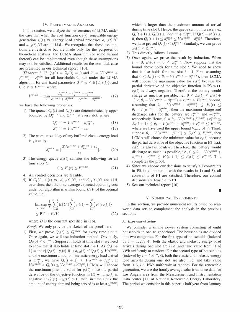
First, we compare our algorithm with the two approaches
above using the real-world solar power data. Note that the
performance of LCMA depends on the battery capacity,
the battery cost, and the control parameters V and ǫi. We
choose b1 = 0.5, Emaxi = 20kWh, i ∈ {1, 2, 3, 4}, and
Emaxi = 30kWh, i ∈ {5, 6, 7, 8}. The initial battery energy
level at each household is chosen to be zero. Let V = Vmax
and ǫi = E{di,2(t)}, ∀i. As can be seen in Figure 2(a),
our proposed LCMA can reduce the total energy cost by
approximately 20% compared with B1 and 13% compared
with B2 in the six-month period. Also, the slopes of the
lines are different, meaning that the savings are unbounded
as the time increases. Secondly, we adjust the battery capacity
and observe the energy cost while setting V = V max. From
Fig. 2(b), we can see that the larger the battery is, the more cost
saving our algorithm can achieve, which matches the analytical
results presented above. More detailed simulation results such
as the delay performance of LCMA and the impacts of battery
cost and ǫi on the performance of LCMA can be found in our
technical report [10].
VI. CONCLUSIONS
In this paper, we present an algorithm (LCMA) for coordi-
nated stochastic optimization of flexible energy resources in
a smart grid setting. The total system cost can be reduced if
more energy loads are elastic and can tolerate being served
with some delay. Our algorithm is simple and was shown to
be able to operate without knowing the statistical properties of
0 800 1600 2400 3200 40000
5
10
15x 10
5
Time (Hours)
Tota
l C
ost (D
olla
rs)
LCMAB2B1
(a)
0 800 1600 2400 3200 40000
2
4
6
8
10
12x 10
5
Time (Hours)
Tota
l C
ost (D
olla
rs)
Ei
max = 20, 30
Ei
max = 30, 40
Ei
max = 40, 50
(b)
Fig. 2. (a) Comparison of the total energy cost in three approaches; (b) Theimpact of battery capacity on the cost saving
the underlying dynamics in the system. With the increase of
energy storage capacities, the performance of our algorithm is
proved to be arbitrarily close to the optimal value. Moreover,
our algorithm provides an explicit relationship between energy
storage capacity, worst-case delay, and cost saving. Extensive
numerical evaluations based on the real-world data show the
effectiveness of our approach.
REFERENCES
[1] A. Ipakchi and F. Albuyeh, “Grid of the future,” Power and Energy
Magazine, IEEE, vol. 7, no. 2, pp. 52–62, 2009.[2] P. Palensky and D. Dietrich, “Demand side management: Demand
response, intelligent energy systems, and smart loads,” Industrial In-
formatics, IEEE Transactions on, vol. 7, no. 3, pp. 381–388, Aug 2011.[3] M. Albadi and E. El-Saadany, “A summary of demand response in
electricity markets,” Electric Power Systems Research, vol. 78, no. 11,pp. 1989–1996, 2008.
[4] H. Farhangi, “The path of the smart grid,” Power and Energy Magazine,
IEEE, vol. 8, no. 1, pp. 18–28, 2010.[5] United States Energy Information Administration. [Online]. Available:
http://www.eia.gov/[6] N. Li, L. Chen, and S. H. Low, “Optimal demand response based on
utility maximization in power networks,” in Power and Energy Society
General Meeting, 2011 IEEE, Detroit, MI, Jul 2011, pp. 1–8.[7] S. Barker, A. Mishra, D. Irwin, P. Shenoy, and J. Albrecht, “Smartcap:
Flattening peak electricity demand in smart homes,” in Proceedings
of the IEEE International Conference on Pervasive Computing and
Communications (PerCom’12), Lugano, Switzerland, Mar 2012.[8] M. Neely, A. Tehrani, and A. Dimakis, “Efficient algorithms for
renewable energy allocation to delay tolerant consumers,” in Smart
Grid Communications (SmartGridComm’10), First IEEE International
Conference on, Washington, DC, Oct 2010, pp. 549–554.[9] M. J. Neely, Stochastic Network Optimization with Application to
Communication and Queueing Systems. San Rafael, CA: Morgan &Claypool Publishers, 2010.
[10] Y. Guo, M. Pan, Y. Fang, and P. P. Khargonekar, “Decentralizedcooridination of energy utilization for residential housholds in the smartgrid,” University of Florida, Tech. Rep., 2012. [Online]. Available:http://plaza.ufl.edu/guoyuanxiong/TSG 12.pdf
[11] NREL: Measurement and Instrumentation Data Center. [Online].Available: http://www.nrel.gov/midc/
126