Embed Size (px)
Citation preview

Cooperative Towing with Multiple Robots
Peng Cheng Jon Fink Vijay Kumar
GRASP Lab
University of Pennsylvania
Philadelphia, PA 19104
Email: {chpeng, jonfink, kumar}@grasp.upenn.edu
Jong-Shi Pang
Department of Industrial and Enterprise Systems Engineering
University of Illinois
Urbana, IL 61801
Email: [email protected]
ABSTRACT
In this paper, we address the cooperative towing of payloads by multiple mobile robots in the plane.
Robots are attached via cables to a planar object or a pallet carrying a payload, and they coordinate
their motion to manipulate the payload through a planar, warehouse-like environment. We formulate a
quasi-static model for manipulation and derive equations of motion that yield the motion of the payload
for a prescribed motion of the robots in the presence of dry friction and tension constraints. We present
experimental results that demonstrate the basic concepts.
1 Introduction
There are many important applications in which vehicles are used to tow payloads using cables or chains.
Conventional oceanographic data collection is largely dependent on towed systems. Tugboats are used to maneu-
ver large boats and ships through rivers and canals. Tow boats are generally used for pushing while tug boats are
used for towing a barge or multiple barges tied together. Helicopters are often used to carry suspended payloads.
In this paper we are primarily interested in cooperative manipulation of payloads by multiple vehicles. Co-
operative lifting of large payloads by multiple helicopters has great benefits in humanitarian or military field

operations. There are advantages to using multiple tugboats for towing. Smaller tugboats which have better ma-
neuverability can be reconfigured to tow large barges depending on their payloads. For warehousing operations,
automatic guided vehicles (AGVs) are generally used for pallets. But pallets can also be towed by AGVs. And if
pallets of different sizes and weights are used, multiple robots can be reconfigured to tow pallets based on the size
and payload.
From the standpoint of robotics, towing is an important manipulation process [1]. However, there are few
studies of robotic towing, especially tasks involving cooperation between multiple robots. The kinematics and
dynamics of cable-actuated, parallel manipulators, which have been studied extensively [2–5], are relevant to this
work. However, this body of literature primarily addresses the control of the cable extensions or forces in order to
manipulate the payload. In contrast, towing involves cables of fixed length where manipulation is accomplished
by controlling the motions of the ”pivot points” in the parallel manipulators. While manipulation using cables
has been studied in the context of distributed manipulation [6–8], these papers do not address the mechanics or
control of the cooperative manipulation task.
Because we address the quasi-static manipulation of objects on a plane the body of work on the mechanics
of objects sliding on a rough plane is very relevant. Because assumptions of rigidity and planar contact are not
compatible in practice, planar surface contact is difficult to model. It has been shown that any planar contact with
dry friction can be modeled by three point contacts [1, 9]. Quasi-static analysis of a planar rigid body on a rough,
horizontal plane reduces to first determining the force distribution in the vertical direction using a three-point-
contact support, and then determining the frictional forces from the motion of the rigid body. However, there is
no canonical three-point-contact support for a rigid body. Further, dry friction is very difficult to model [10].
Finally, the unilateral constraints imposed by cables that can only admit positive forces introduce another
degree of complexity into the problem. Because the tension on a cable can only be positive and the distance
between the two end-points of a cable cannot be more than its free length, and further the tension is non zero only
when the distance is equal to the free lengths – each cable introduces a complementarity constraint of the type:
s≥ 0, λ≥ 0, λ s = 0 (1)
where s is the slack in the cable and λ is the tension in the cable. The solutions to systems of linear equations sub-
ject to such constraints, the so-called Linear Complementarity Problem (LCP), have been studied extensively [11].
Even though all the terms in the LCP are linear in the unknowns, the system can have multiple solutions or no
solutions at all. In addition to having complementarity constraints, the planar towing problem considered here has

Initial configuration
Goal configuration
Towing robots
Static obstacles
Fig. 1. Multiple cooperative manipulation by towing
frictional constraints which are nonlinear.
In this paper, we first formulate a quasi-static model of towing planar objects with multiple robots in Section 2.
A key assumption in this section is the three-point-contact support model which is realized in our experimental
testbed by supporting the payload on three castors. In Section 3, we present an analysis of the instantaneous
kinematics conditions for the existence of a unique object twist. We next explore the set of configurations in which
a system with a three-point-contact support can be quasi-statically towed using multiple robots in Section 4. In
Section 5, we show experimental results with a system of position-controlled robots towing a payload. The robots
have no force sensors and must coordinate their relative velocities to achieve a desired twist. We show that
our model correctly predicts the resulting motion. Finally, in Section 6, we outline a few open problems in the
kinematics, planning and control of cooperative towing, and extensions of the research described here.
2 The Quasi-Static Model for Cooperative Towing
Our task is to control multiple robots so they can cooperatively tow or carry a planar object subject to gravity
and frictional forces from any initial part configuration to a desired goal part configuration. We want to avoid
obstacles as shown in Fig. 1 and achieve a specified degree of precision in positioning and orienting the object at
a desired final position and orientation.
The different variables characterizing a robot towing a payload are shown in Fig. 2. The position and orienta-
tion of the payload is given by (x,y,θ). The velocity of the payload is a twist (in the plane), which can be written

S3
S2
(x, y)!
"1s1
Ob
xw
yw
Ow
xb
yb
S1
Pj#j
rj
Rj
uj
vRj
New
figure 3
S3 S
2
S1
!n,1
!n,3
!n,2
!t,1
!t,2
!t,3
!c,jPj
Ob
mg
Fig. 2. Quasi-static manipulation: The object is supported by three support points, Si, with normal forces (out of the plane), λn,i and
tangential frictional forces, λt,i. It is pulled by m cables, each exerting a force λc, j . Note the robot R j pulls by moving the object with a
prescribed (given) velocity.
in the world frame:
ξ =
x
y
θ
. (2)
Even though the following modeling and analysis on the twist are in the world frame, they can be easily extended
for the twist in the body-fixed frame by using the rotation matrix to transform quantities in the world frame into
the body-fixed frame. We have used this to maintain the twist in the body-fixed frame in our experiments as shown
in Section 5.
Let xR, j = (xR, j,yR, j) denote the position of the reference point R j on robot j. If there are m robots with
cables attached to points R j on robot j and Pj on the payload, and if∣∣∣−−→PjR j
∣∣∣ equals the free length of the cable, the
unilateral kinematic constraints associated with cables are:
Aξ≥ 1b (3)
where
A =
A1
. . .
Am
, b =
b1
. . .
bm
, (4)
1this vector inequality denotes that each element of the vector satisfies the inequality
A j is a function of the unit vector, u j, showing the direction of the cable j and the position vector ρ j =−−→ObP j:
ATj =
u j
ρ j×u j
, (5)
b j is a function of u j and the velocity vR, j of the towing robot j:
b j = uTj vR, j. (6)
Note that b j ∈ [−vmaxR ,vmax
R ] because the robot velocity vR, j is bounded by vmaxR .
The set of twists of freedom is defined with respect to the tuple (A,b) as follows:
Σ(A,b) = {ξ |Aξ ≥ b}. (7)
Note that this set is determined by the configuration of the robots, specified by the matrix A, and the payload as
well as the velocities of the robots, given by the vector b.
The kinematics-statics duality is evident in this problem. There are similarly constraints on the cable tensions.
λc, the m× 1 vector of cable tensions, is non negative and is non zero only when the equality in (3) is satisfied.
Thus we write complementarity constraints:
0≤ λc ⊥ Aξ−b≥ 0, (8)
where “⊥” implies λc, j(Aξ−b) j = 0. Since λc and Aξ−b are non negative, λTc (Aξ−b) = 0.
In order to model the dry friction between the object and the support surface, we assume that the object is
supported by a finite number of frictional point contacts. For three non collinear support points, the support forces
λn,i, i = 1,2,3 can be uniquely obtained.
If the object undergoes quasi-static motion, the tensions associated with m cables and the frictional forces
(λt,i,x,λt,i,y) at each of the three support points (i = 1,2,3) must add to zero. Thus, we have the equilibrium

equations:
BTλt +AT
λc = 0, λc ≥ 0 (9)
where B is a full rank 6×3 matrix:
BT =[
BT1 BT
2 BT3
]=
1 0 1 0 1 0
0 1 0 1 0 1
−ys,1 xs,1 −ys,2 xs,2 −ys,3 xs,3
, Bi =
1 0 −ys,i
0 1 xs,i
, (10)
and λt is a 6×1 unknown vector:
λt = [λTt,1, λ
Tt,2, λ
Tt,3]
T , λt,i = [λt,i,x, λt,i,y]T . (11)
We use F C i to denote the friction cone at the ith support point defined by Coulomb friction:
0≤ ‖λt,i‖ ≤ µλn,i, ‖λt,i‖=√
λ2t,i,x +λ2
t,i,y. (12)
Note that F C i is the friction cone with a known λn,i.
For a given object twist, the 2×1 velocity vector of the support point is given by:
vt,i = Bi ξ =
1 0 −ys,i
0 1 xs,i
ξ.
From Coulomb’s law, the friction forces are equal to µλn,i and are opposite to the direction of slip, except if the
slip is zero when the magnitude is indeterminate. This can be written explicitly as:
λ t,i(ξ) ∈ argminλ t,i∈F C i
vt,i(ξ)Tλ t,i,
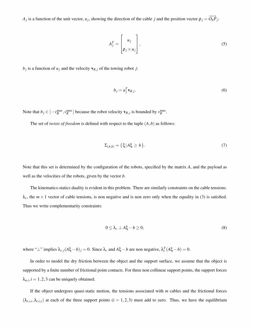
or in aggregate form,
λ t(ξ) ∈ argminλ t,i∈F C i
ξT BT
λ t . (13)
It is not too hard to verify that this is equivalent to the Coulomb friction law [12].
3 Existence and Uniqueness of Solutions to (8), (9), and (13)
In this section, we will study the quasi-static model in Section 2, specifically addressing the existence and
uniqueness of solutions to (8), (9), and (13) by considering the following max-min problem:
maximizeξ∈Σ(A,b)
minimizeλ t,i∈F C i
L(ξ,λ t) (14)
with the saddle function L(ξ,λ t) ≡ ξT BT λ t being bilinear in its arguments. We say that a pair (ξ,λ t) is feasible
if ξ satisfies the kinematic constraint (3) and λ t satisfies the friction constraints: λ t,i ∈ F C i for all i = 1,2,3. By
definition, a feasible pair (ξ, λ t) is a saddle point of L if for all feasible pairs (ξ,λ):
L(ξ,λ t) ≥ L(ξ, λ t) ≥ L(ξ, λ t). (15)
It is known [13, Theorem 1.4.1] that the following three statements are equivalent:
(a) (ξ, λ t) is a saddle point of L over the feasible pairs of admissible twists and friction forces;
(b) ξ ∈ argmaxξ∈Σ(A,b)
ϕ(ξ) and λ t ∈ argminλ t,i∈F C i
ψ(λt), where
ϕ(ξ) ≡ minλ t,i∈F C i
L(ξ,λ t) and ψ(λ t) ≡ maxξ∈Σ(A,b)
L(ξ,λ t);
(c) ϕ(ξ) = ψ(λ t) = L(ξ, λ t).
The existence and uniqueness of a solution to the quasi-static towing problem formulated in (8), (9), and (13) are
established in two steps: (a) such a solution is characterized as a saddle point of L in (14); and (b) such a saddle
point exists and is unique. The result below establishes the first step.

Theorem 1. A feasible pair (ξ, λ t) is a saddle point of L if and only if λc exists such that the triple (ξ, λ t , λc)
satisfies conditions (8), (9), and (13).
Proof. The right-hand inequality in (15) holds if and only if ξ maximizes L(•, λ t) over the set Σ(A,b). In turn,
since the latter maximization is a linear program in the variable ξ ∈ Σ(A,b), it follows that the right-hand inequality
in (15) holds if and only if λc exists such that (ξ, λ t , λc) satisfies conditions (8) and (9). Clearly, the left-hand
inequality in (15) is just (13). �
To proceed to the second step, notice that
ϕ(ξ) =3
∑i=1
minimizeλt,i∈F C i
{(Biξ)T
λ t,i}
= −3
∑i=1
µλn,i
√(x− ys,iθ
)2 +(
y+ xs,iθ)2
The next result is based on the maximization problem of ϕ(ξ) over Σ(A,b).
Theorem 2. Suppose that Σ(A,b) is not empty (i.e., there exists a twist that satisfies the kinematic constraint in
(3)) and that B ∈ R6×3 is full rank. There exists a unique ξ and possibly non unique (λ t , λc) such that (ξ, λ t , λc)
satisfies the conditions (8), (9), and (13); moreover, ξ is the unique solution of the problem:
minimizeξ=(x,y,θ)
−ϕ(ξ)
subject to Aξ ≥ b
(16)
and for i = 1,2,3, λ t,i ∈ argminλ t,i∈F C i
vt,i(ξ)Tλ t,i.
Proof. The minimization problem (16) is clearly equivalent to the maximization problem of ϕ(ξ) over Σ(A,b). The
objective function of (16), −ϕ(ξ), is a coercive function of ξ, i.e.,
lim‖ξ‖→∞
−ϕ(ξ) = ∞.
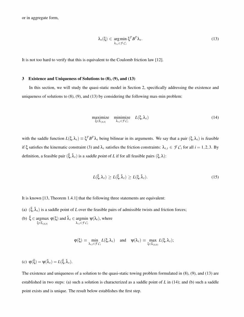
This is because B is full rank and the coefficients µ and λn,i are positive. Since −ϕ(ξ) is a continuous, coercive
function of ξ and the polyhedron Σ(A,b) is a closed set, an optimal solution to (16) is guaranteed [14].
To show the uniqueness of such an optimal solution, let ξi ≡ (xi, yi, θi) be two optimal solutions. Since−ϕ(ξ)
is a convex function, it follows that
ϕ(τξ1 +(1− τ)ξ2) = ϕ(ξ1) = ϕ(ξ2), ∀τ ∈ [0,1],
which implies
‖vt,i(τξ1 +(1− τ)ξ2)‖ = ‖vt,i(ξ1)‖ = ‖vt,i(ξ2)‖, ∀τ ∈ [0,1].
Hence, Biξ1 = Biξ
2 for i = 1,2,3, and hence ξ1 = ξ2 by the same full rank condition of B.
With ξ denoting the unique optimal solution of (16), it follows that λc exists such that (ξ, λc) satisfies (8) and
0 ∈ −AT λc−∂ϕ(ξ), where −∂ϕ(ξ) denotes the subdifferential of the convex function −ϕ at ξ. Since
−ϕ(ξ) =3
∑i=1
µλn,i ‖Biξ‖,
we have
−∂ϕ(ξ) =3
∑i=1
µλn,i BTi (∂‖v‖)v=Biξ
=3
∑i=1
µλn,i BTi
{
Biξ
‖Biξ‖
}if Biξ 6= 0
F C i/(µλn,i) if Biξ = 0
= −BT λ t .
Thus, (ξ, λ t , λc) satisfies (8), (9), and (13). �

Remark: The optimization problem (16) is a convex program. Indeed, it is equivalent to a non-standard linear
program over a second-order cone:
minimizeξ=(x,y,θ),σ
3
∑i=1
µλn,i σi
subject to Aξ ≥ b
and σi =√(
x− ys,iθ)2 +
(y+ xs,iθ
)2 ≤ σmaxi , for i = 1,2,3.
(17)
where σmaxi is a positive upper bound for the sliding velocity at the support point i. This is a problem that has been
extensively studied in the recent mathematical programming literature; see e.g. [15]. We use standard Matlab c©
functions to solve (14) for the object twist to generate the results shown in Section 5.
4 Control of Object Twists
In this section, we will study when admissible twists exist for a towing configuration A, whether there exist
inadmissible twists that cannot be produced by a group of robots, and how to coordinate the robots to achieve a
desired twist.
4.1 Admissible and inadmissible object twists
We will first study conditions on A to ensure the existence of an object twist and whether there exist inadmis-
sible twists for three robots.
Theorem 3 below shows that there exists a unique admissible twist if A is full rank and m≤ 3.
Theorem 3. If A is full rank and m≤ 3, then there always exists a unique twist ξ to the towing problem formulated
in (8), (9), and (13).
Proof: Stiemke’s lemma is a theorem of alternatives that states that one of the following two conditions is true:
Either
∃λc > 0, ATλc = 0. (18)
or,
∃ξ : A ξ > 0. (19)
If A is full rank and m≤ 3, (18) is not true. Therefore there must exist twists that satisfy the constraint (19). For
any given b, if elements b j ≤ 0, (19) implies the constraint A jξ≥ b j is satisfied. If there are elements b j > 0, then
we can always scale ξ with a positive scalar so that a feasible ξ that satisfies A jξ≥ b j can be found. Thus, Σ(A,b)
is not empty. Theorems 1 and 2 guarantee that there always exists a unique part twist ξ for (8), (9), and (13). �
Remark It is well known that if a wrench w is applied on an object moving on a plane with a twist t, the rate at
which work is done is given by wT t provided the elements of the twist and wrench are written as follows:
w =
fx
fy
mz
, t =
x
y
θ
(20)
The rate of work done by all the wrenches on the towed object must be zero, which means:
λTc Aξ+λ
Tt Bξ = 0. (21)
We know that λTt Bξ≤ 0 because this term is associated with the rate of work done by frictional forces which must
be non positive. Also ξ 6= 0 if and only if
λTt Bξ < 0. (22)
Thus, if ξ 6= 0, from (21) we have
λTc Aξ > 0. (23)

The strict inequality means that at least one cable is pulling the object.
From Theorem 3, when A is full rank with m ≤ 3, different twists can be produced by changing the robot
velocities to generate different b vectors. However, the following theorem shows that for three or fewer robots
with specified lines of action of the cables, there always exist inadmissible twists that cannot be produced no
matter what the robot velocities are.
Theorem 4. If A is full rank and m≤ 3, not all twists can be produced.
Proof: From Stiemke’s lemma, either
∃λc > 0,−ATλc = 0. (24)
or,
∃ξ : −A ξ > 0. (25)
If A is full rank and m≤ 3, (24) is not true. This means (25) must be true, or equivalently,
∃ξ : A ξ < 0.
Therefore, there exist twists that violate (23) because λc ≥ 0. �
4.2 Producing any twist with more than three robots
We have shown that there exist inadmissible twists that cannot be produced by three robots. However, with a
fourth robot, we can produce any twist up to scale as shown in the following theorem.
Theorem 5. Given four towing robots and any part twist ξdes, we can find β ∈ (0,1) and (A,b) such that
ξ = βξdes (26)
is the unique solution to (14).
Proof: We will first prove that there exists a matrix A for four robots such that ξdes can be produced if the robots
can move arbitrarily fast. Secondly, we will show that there exist b and ξ = βξdes for 0 < β < 1 such that ξ can be
produced even though there exist upper bounds on the robot velocities.
Step 1: Again we use Stiemke’s lemma in the form of (24) and (25). We will construct the matrix A for four
robots satisfying (24) such that all twists can be produced. This is done by selecting A j, the lines of action for the
cables or the rows of A, such that the four submatrices, D1 = [AT2 AT
3 AT4 ], D2 = [AT
1 AT3 AT
4 ], D3 = [AT1 AT
2 AT4 ], and
D4 = [AT1 AT
2 AT3 ] satisfy the following properties.
(a) All submatrices are full rank; and
(b) −det(D1), det(D2), −det(D3), and det(D4) have the same sign.
According to [4, Corollary 3.4] , (24) has a solution if and only if the above conditions are satisfied.
In the following, we will show that there exists a matrix A satisfying the above conditions. We can first select
any three non parallel and non concurrent cable directions. Without losing generality, we assume these cables are
respectively for robots 1,2 and 3. It can be checked that the resulting submatrix D4 is full rank. Then, there exist
αi < 0 for i = 1,2, and 3 such that q = [q1 q2 q3]T = α1A1 +α2A2 +α3A3 with q21 +q2
2 6= 0. It can be checked that
choosing A4 of the fourth robot as
A4 =q√
q21 +q2
2
=α1√
q21 +q2
2
A1 +α2√
q21 +q2
2
A2 +α3√
q21 +q2
2
A3
will ensure the above two conditions. The first two elements of A4 determine the cable direction u4 and the third
element determines a straight line set in which the anchor point on the part can be chosen.
Thus, such matrix A guarantees that (25) is not true. In other words, there is no twist such that Aξ < 0.
Alternatively, for all twists, including ξdes, the opposite must be true:
Aξdes ≥ 0.
In other words, ξdes can be produced with bdes = Aξdes, which can always be achieved if there are no constraints
on the speed of the robots.

Step 2: If the robot speed is bounded by vmaxR , for any ξdes we can always find
β ∈
0,min
vmaxR
maxj=1,2,3,4
|A jξdes|
,1
(27)
such that the scaled twist, ξ = β ξdes, can be produced by robot velocities vR, j given by:
vR, j ·u j = A j
(β ξ
des)
, j = 1,2, . . . ,m. (28)
�
5 Experiments and Verification
In this section, we will present our experimental results to validate the proposed model for the system of
cooperating robots. We present results for one, two and three robots towing an object. We also show that the
robots are able to produce desired twists in the body-fixed frame leading to desired motions corresponding to
one-parameter subgroups in the Euclidean group in two dimensions.
5.1 Experimental testbed
All experiments were conducted on a multi-robot testbed [16] utilizing a team of small differential drive robots
(radius 0.15m) called Scarabs, and an overhead tracking system for localization of both the manipulated object
and the robots. Each Scarab is equipped with a differential drive axle placed at the center of the length of the
robot with a 21 cm wheel base. The robot is driven by two low-power stepper motors which each drive 10 cm
(standard rubber scooter) wheels with a gear reduction (using timing belts) of 4.4:1, resulting in a nominal holding
torque of 28.2kg-cm at the axle. Each robot has an on-board computer equipped with a Nano ITX motherboard
with a 1 GHz. processor and 1 GB of RAM. A compact flash drive provides low-energy data storage in place of
a hard drive. A power management board and smart battery provide approximately two hours of experimentation
time (under normal operating conditions). The on-board embedded computer supports two IEEE 1394 devices
and 802.11a/b/g wireless communication. The sensors, actuators, and controllers are modular and connected
through the Robotics Bus [17] (which is derived from the CAN bus protocol) or standard interfaces such as USB
or IEEE 1394. The result is a plug-and-play system where sensors and actuators can be added or removed from

Fig. 3. The Scarab platform used for experiments and a photograph showing three Scarabs towing a payload.
the hardware configuration. More details are available in [16].
The Scarab robot in Fig. 3 depicts a typical platform configuration with a Hokuyo URG laser range finder
and a Point Grey Firefly IEEE 1394 camera. A foam bumper protects the robot while allowing it to physically
interact with its environment. The physical dimensions of the robot in this configuration (less the bumper) are
20×13.5×22.2 cm3 with a mass of 8 kg.
5.2 System parameters
In Fig. 3 (right), the robots are manipulating an L-shaped object with a characteristic length of 1m, mass of
2.5Kg, and an approximate coefficient of friction with the floor of µs = 0.08. The low coefficient of friction is
due to the rolling friction at the castors. The castors also help reduce the uncertainties associated with the force
distribution. If there were no castors, the problem of determining the normal support forces for a planar rigid body
resting on a plane has infinite solutions.
The robots are connected to the object through fixed length cables (0.75m) which are fastened to known
attachment points on both the object and robot. Since the robots are actuated by a differential drive system, they
have nonholonomic constraints and we simplify the control problem by controlling the point R j at which the cable
is attached using a standard feedback linearization scheme [18]. This point is chosen to be at a 0.09m offset from
robot axle to guarantee input-output linearization.
For these experiments, we assume our tracking system has an accuracy of ±2cm and ±5◦. For our estimation
of the towing configuration, A, from experimental trajectories, we depend on the difference between two measure-
ments and thus the assumed error on these values is doubled. A centralized clock is used so we assume timing
error to be negligible.
-1.5 -1.0 -0.5 0.0 0.5
-0.5
0.0
0.5
1.0
(a)
6 6.5 7 7.5 8 8.5 9 9.5 10 10.5 11−0.2
0
0.2Predicted/Actual Velocity Error
X E
rror
(m
/s)
6 6.5 7 7.5 8 8.5 9 9.5 10 10.5 11−0.2
0
0.2
Y E
rror
(m
/s)
6 6.5 7 7.5 8 8.5 9 9.5 10 10.5 11−5
05
1015
θ E
rror
(de
g/s)
Time (s)
(b)
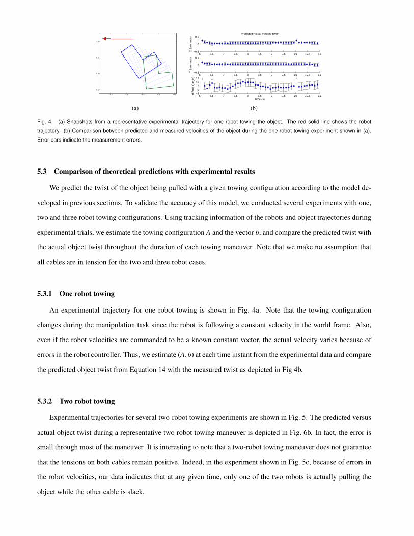
Fig. 4. (a) Snapshots from a representative experimental trajectory for one robot towing the object. The red solid line shows the robot
trajectory. (b) Comparison between predicted and measured velocities of the object during the one-robot towing experiment shown in (a).
Error bars indicate the measurement errors.
5.3 Comparison of theoretical predictions with experimental results
We predict the twist of the object being pulled with a given towing configuration according to the model de-
veloped in previous sections. To validate the accuracy of this model, we conducted several experiments with one,
two and three robot towing configurations. Using tracking information of the robots and object trajectories during
experimental trials, we estimate the towing configuration A and the vector b, and compare the predicted twist with
the actual object twist throughout the duration of each towing maneuver. Note that we make no assumption that
all cables are in tension for the two and three robot cases.
5.3.1 One robot towing
An experimental trajectory for one robot towing is shown in Fig. 4a. Note that the towing configuration
changes during the manipulation task since the robot is following a constant velocity in the world frame. Also,
even if the robot velocities are commanded to be a known constant vector, the actual velocity varies because of
errors in the robot controller. Thus, we estimate (A,b) at each time instant from the experimental data and compare
the predicted object twist from Equation 14 with the measured twist as depicted in Fig 4b.
5.3.2 Two robot towing
Experimental trajectories for several two-robot towing experiments are shown in Fig. 5. The predicted versus
actual object twist during a representative two robot towing maneuver is depicted in Fig. 6b. In fact, the error is
small through most of the maneuver. It is interesting to note that a two-robot towing maneuver does not guarantee
that the tensions on both cables remain positive. Indeed, in the experiment shown in Fig. 5c, because of errors in
the robot velocities, our data indicates that at any given time, only one of the two robots is actually pulling the
object while the other cable is slack.
-0.5 0.0 0.5 1.0 1.5 2.0 2.5 3.0
-1.0
-0.5
0.0
0.5
1.0
(a)
-0.5 0.0 0.5 1.0-0.6
-0.4
-0.2
0.0
0.2
0.4
0.6
0.8
1.0
(b)
-1.5 -1.0 -0.5 0.0 0.5 1.0 1.5 2.0-2.0
-1.5
-1.0
-0.5
0.0
0.5
1.0
(c)
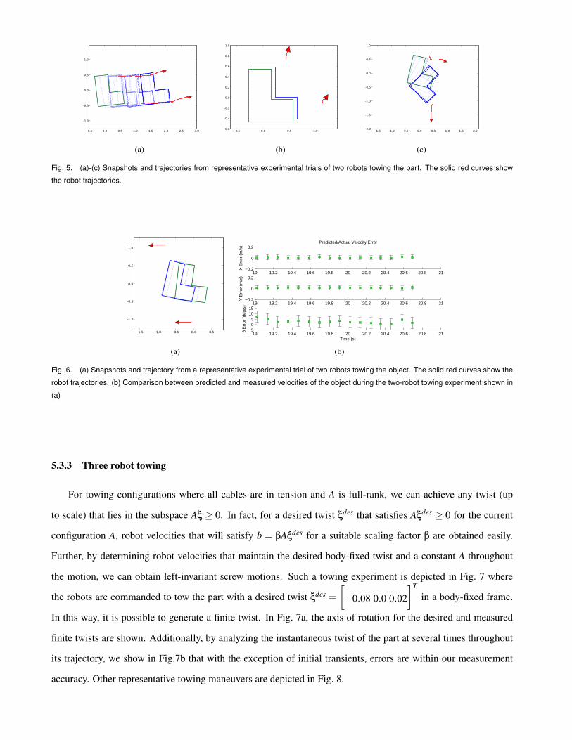
Fig. 5. (a)-(c) Snapshots and trajectories from representative experimental trials of two robots towing the part. The solid red curves show
the robot trajectories.
-1.5 -1.0 -0.5 0.0 0.5
-1.0
-0.5
0.0
0.5
1.0
(a)
19 19.2 19.4 19.6 19.8 20 20.2 20.4 20.6 20.8 21−0.2
0
0.2Predicted/Actual Velocity Error
X E
rror
(m
/s)
19 19.2 19.4 19.6 19.8 20 20.2 20.4 20.6 20.8 21−0.2
0
0.2
Y E
rror
(m
/s)
19 19.2 19.4 19.6 19.8 20 20.2 20.4 20.6 20.8 21−5
05
1015
θ E
rror
(de
g/s)
Time (s)
(b)
Fig. 6. (a) Snapshots and trajectory from a representative experimental trial of two robots towing the object. The solid red curves show the
robot trajectories. (b) Comparison between predicted and measured velocities of the object during the two-robot towing experiment shown in
(a)
5.3.3 Three robot towing
For towing configurations where all cables are in tension and A is full-rank, we can achieve any twist (up
to scale) that lies in the subspace Aξ ≥ 0. In fact, for a desired twist ξdes that satisfies Aξdes ≥ 0 for the current
configuration A, robot velocities that will satisfy b = βAξdes for a suitable scaling factor β are obtained easily.
Further, by determining robot velocities that maintain the desired body-fixed twist and a constant A throughout
the motion, we can obtain left-invariant screw motions. Such a towing experiment is depicted in Fig. 7 where
the robots are commanded to tow the part with a desired twist ξdes =[−0.08 0.0 0.02
]T
in a body-fixed frame.
In this way, it is possible to generate a finite twist. In Fig. 7a, the axis of rotation for the desired and measured
finite twists are shown. Additionally, by analyzing the instantaneous twist of the part at several times throughout
its trajectory, we show in Fig.7b that with the exception of initial transients, errors are within our measurement
accuracy. Other representative towing maneuvers are depicted in Fig. 8.

-1 0 1 2 3
X Position (m)
-1
0
1
2
3Y
Posit
ion
(m
)
Axes of rotationAcheived
Desired
(a)
0 5 10 15 20 25 30 35 40 45−0.1
0
0.1
0.2
0.3Twist Error
x (m
/s)
0 5 10 15 20 25 30 35 40 45−0.05
0
0.05
0.1
0.15
y (m
/s)
0 5 10 15 20 25 30 35 40 45−0.1
0
0.1
0.2
0.3
θ (r
ad/s
)
Time (s)
(b)
Fig. 7. (a) Plot of part trajectory while being towed along a desired twist by three robots. The desired and measured rotation axes are shown
in the upper left. (b) Error on instantaneous twist components with error bars showing the measurement accuracy of our tracking system
-1.0 -0.5 0.0 0.5 1.0 1.5 2.0
-1.0
-0.5
0.0
0.5
(a)
-1.5 -1.0 -0.5 0.0 0.5-1.5
-1.0
-0.5
0.0
0.5
(b)
-1.0 -0.5 0.0 0.5 1.0 1.5-1.0
-0.5
0.0
0.5
1.0
1.5
(c)
Fig. 8. (a)-(c) Snapshots and trajectories from representative experimental trials of three robots towing the part. The solid red curves show
the robot trajectories.
6 Conclusion
In this paper, we studied the mechanics of planar, multi-robot towing in which multiple robots tow a planar
payload subject to friction. The problem formulation incorporates complementarity constraints which are neces-
sary to allow for cables becoming slack during a towing maneuver. We established the uniqueness and existence
for the solutions to the forward dynamics problems using a max-min problem formulation. We also showed that
three robots cannot produce arbitrary desired twists, however, four robots are able to produce any twist up to
scale. By controlling the robots to produce such an arbitrary desired twist in a body-fixed frame, any left-invariant
(screw) motion can be produced. Further, the payload can be towed along any prescribed path in the plane.
The experimental results presented in this paper show that it is necessary to model transitions between non
zero tension and zero tension using the complementarity formulation. It is impossible to maintain non zero
tensions without force sensors and we expect cables to exhibit transitions. Even so, the experimental data shows
consistency with the theoretical predictions.
There are three avenues for future research, all of which are being pursued independently. First, from a design
perspective, it is necessary to introduce compliance into the cables. Rigid cables result in cable tensions changing
from positive values to zero values introducing non smoothness. Compliance is also necessary to analyze sys-
tems with more than three robots. Secondly, from a control perspective, it is necessary to incorporate feedback
of robot and object information to allow the robots to coordinate their motion and to follow desired object tra-
jectories. Because of the inevitable errors in coordinating robot motions and the uncertainty in support friction,
we are particularly interested in analyzing the case where more than three castors (typically four are used for a
pallet) are used and designing planning and control strategies that are effective for towing payloads in a cluttered
environment. Finally, it is useful to consider the extension to problems in which inertial effects are significant.
The uniqueness and existence issues are likely to be simpler because of the existence of a positive-definite inertia
matrix. However, the coordinated control of the robots is more difficult.
Acknowledgement
We gratefully acknowledge the support of NSF grants DMS01-39747, DMS-075437, IIS02-22927, and IIS-
0413138, and ARO grant W911NF-04-1-0148.
References
[1] Mason, M. T., 2001. Mechanics of robotic manipulation. MIT Press.
[2] Oh, S., and Agrawal, S., 2003. “Cable-suspended planar parallel robots with redundant cables: Controllers
with positive cable tensions”. In Proc. of IEEE International Conference on Robotics and Automation,
pp. 3023–3028.
[3] Bosscher, P., and Ebert-Uphoff, I., 2004. “Wrench based analysis of cable-driven robots”. In Proceedings of
the IEEE International Conference on Robotics and Automation, pp. 4950–4955.
[4] Stump, E., and Kumar, V., 2006. “Workspaces of cable-actuated parallel manipulators”. ASME Journal of
Mechanical Design, 128, January.
[5] Verhoeven, R., 2004. “Analysis of the workspace of tendon-based stewart platforms”. PhD thesis, University
of Duisburg-Essen.
[6] Donald, B. R., Gariepy, L., and Rus, D., 2000. “Distributed manipulation of multiple objects using ropes”.
In Proceedings IEEE International Conference on Robotics & Automation.
[7] Donald, B. R., 1995. “On information invariants in robotics”. Artificial Intelligence Journal, 72, pp. 217–
304.

[8] Donald, B. R., 1997. “Information invariants for distributed manipulation”. International Journal of Robotics
Research, 16.
[9] Peshkin, M. A., 1986. “Planning robotic manipulation strategies for sliding objects”. PhD thesis, Carnegie
Mellon University Department of Physics, November.
[10] Goyal, S., Ruina, A., and Papadopolous, J., 1989. “Limit surface and moment function descriptions of planar
sliding”. pp. 794–799.
[11] Cottle, R. W., Pang, J., and Stone, R. E., 1992. The Linear Complementarity Problem. Academic Press.
[12] Anitescu, M., and Potra, F. A., 2002. “A time-stepping method for stiff multibody dynamics with contact
and friction”. International Journal of Numerical Methods Engineering, July, pp. 753–784.
[13] Facchinei, F., and Pang, J. S., 2003. Finite-dimensional Variational Inequalities and Complementarity Prob-
lems. Springer-Verlag, New York.
[14] Bertsekas, D. P., 1989. Constrained Optimization and Lagrange Multiplier Methods. Academic Press, New
York, NJ.
[15] Boyd, S., and Vandenberghe, L., 2004. Convex Optimization. Cambridge University Press.
[16] Michael, N., Fink, J., and Kumar, V., 2008. “Experimental testbed for large multi-robot teams: Verification
and validation”. IEEE Robotics and Automation Magazine, Mar.
[17] Gomez-Ibanez, D., Stump, E., Grocholsky, B., Kumar, V., and Taylor, C. J., 2004. “The robotics bus: a local
communications bus for robots”. In Mobile Robots, D. W. Gage, ed. pp. 155–163.
[18] Murray, R. M., Li, Z., and Sastry, S., 1994. A Mathematical Introduction to Robotic Manipulation. CRC
Press, Boca Raton, FL.