Cooperative project for CFD prediction of pedestrian … · and Industrial Aerodynamics 95 (2007) 1551–1578 Cooperative project for CFD prediction of pedestrian wind environment

ARTICLE IN PRESS

Journal of Wind Engineering

and Industrial Aerodynamics 95 (2007) 1551–1578

0167-6105/$ -

doi:10.1016/j

�CorrespoE-mail ad

www.elsevier.com/locate/jweia

Cooperative project for CFD predictionof pedestrian wind environment in the

Architectural Institute of Japan

R. Yoshiea,�, A. Mochidab, Y. Tominagac, H. Kataokad,K. Harimotoe, T. Nozuf, T. Shirasawag

aDepartment of Architecture, Tokyo Polytechnic University, 1583 Iiyama, Atsugi, Kanagawa 243-0297 JapanbGraduate School of Engineering, Tohoku University, Japan

cNiigata Institute of Technology, JapandTechnical Research Institute, Obayashi Corp., Japan

eTechnology Center, Taisei Corp., JapanfInstitute of Technology, Shimizu Corp., Japan

gThe University of Tokushima, Japan

Available online 23 April 2007

Abstract

CFD (computational fluid dynamics) is being increasingly applied to the prediction of the wind

environment around actual high-rise buildings. Despite this increasing use, the prediction accuracy

and many factors that might affect simulation results are not yet thoroughly understood. In order to

clarify ambiguities and make a guideline for CFD prediction of the wind environment, a working

group was organized by the Architectural Institute of Japan. This group has carried out various

comparative studies as follows.

�
First stage: Flow fields around two types of single high-rise buildings.
�
Second stage: Flow field around a high-rise building located in a city.
�
Last stage: Flow fields around two types of Building Complexes in actual urban areas.
This paper describes some of the results of the investigation by the working group, and discusses

the influences of various calculation conditions on CFD results, and also on the present status and

the problems in CFD prediction of the wind environment.

r 2007 Elsevier Ltd. All rights reserved.

Keywords: CFD; Pedestrian wind environment; RANS model; Guideline

see front matter r 2007 Elsevier Ltd. All rights reserved.

.jweia.2007.02.023

nding author. Tel./fax: +81 46 2429545.

dresses: [email protected] (R. Yoshie), [email protected] (Y. Tominaga).

www.elsevier.com/locate/jweia

dx.doi.org/10.1016/j.jweia.2007.02.023

mailto:[email protected]

mailto:[email protected]

ARTICLE IN PRESS

Nomenclature

U average wind velocity in stream-wise direction (x direction), m/sV average wind velocity in transverse direction (y direction), m/sW average wind velocity in vertical direction (z direction), m/sk Turbulent kinetic energy, m2/s2

� Dissipation rate of turbulent kinetic energy, m2/ s3

Pk Production of turbulent kinetic energy, m2/s3

R. Yoshie et al. / J. Wind Eng. Ind. Aerodyn. 95 (2007) 1551–15781552

1. Introduction

Progress in high-speed processing by personal computer and rapid propagation ofsoftware for numerical analysis of fluid dynamics in recent years have enabled predictionof the pedestrian wind environment around high-rise buildings based on CFD(computational fluid dynamics). It is becoming common for calculations to be performedfor 16 wind directions of the situation before and after construction of proposed buildings,and for the pedestrian wind environment to be assessed by probability evaluation.However, there have been very few reports on the prediction accuracy of CFD simulationsof the pedestrian wind environment around buildings in urban areas. Furthermore, theinfluences of various calculation conditions (such as size of computational domain, gridresolution, boundary conditions, selection of turbulence model, etc.) on the results of CFDsimulation are not yet thoroughly understood.Thus, a working group named ‘‘Working Group for CFD Prediction of the Wind

Environment around a Building’’ has been organized by the Architectural Institute ofJapan. The name of this working group has been subsequently changed to ‘‘WorkingGroup for Preparation of Wind Environment Evaluation Guideline based on CFD’’.Since its inception, it has been making continuous efforts to prepare guidelines for properuse of CFD for calculation of the wind environment. Comparative and parametric studieshave been carried out on several building configurations to elucidate the problems onsetting or selecting various calculation conditions and turbulence models for CFDsimulation of the pedestrian wind environment in urban areas. Although there have beenthe recommendations with similar objectives proposed by COST group (Franke et al.,2004), those are mainly based on the results published by other authors. On the otherhand, we are intended to propose the guidelines based on the results of our ownbenchmark tests.The present article introduces some of the results achieved by the working group and

discusses the influence of calculation conditions and turbulence models on CFDcalculation results and also on the present status and problems in CFD prediction ofthe pedestrian wind environment around buildings.

2. General features of comparative and parametric studies

Figs. 1–6 show models for comparative and parametric studies as investigated by theworking group. The results of studies will be introduced here on the flow field around asingle square prism of 2:1:1 (height:width:depth) placed in a turbulent boundary layer

ARTICLE IN PRESS

H = 2b

b

Wind

b

Fig. 1. Single high-rise building (2:1:1 square prism).

b

4b

4b

b

4b

4b

wind

Fig. 2. Single high-rise building (4:4:1 square prism).

wind

Z

Y

X 0.2m 0.2m0.2m

0.2m

Fig. 3. Simple city block.

Fig. 4. A high-rise building in city.

R. Yoshie et al. / J. Wind Eng. Ind. Aerodyn. 95 (2007) 1551–1578 1553

ARTICLE IN PRESS

Fig. 5. Building complexes in actual urban areas (Niigata).

Fig. 6. Building complexes in actual urban areas (Shinjuku).


flow (Fig. 1), the flow field around a high-rise building located in a city (Fig. 4), and flowfields around building complexes in actual Urban areas in Niigata and Shinjuku, Japan(Figs. 5 and 6).In the studies discussed here, the standard k–� model or modified k–� models or DSM

were used, but LES (large eddy simulation) was not applied except for flow fields aroundtwo types of single prisms (Figs. 1 and 2). It is desirable to use LES for highly accurateCFD. However, it is very difficult to use because it requires a lot of time for calculation inpractical analysis due to the limited conditions of computer resources currently available.This is because, prediction and evaluation of the wind environment around buildings inpractical application requires a wide computational domain including surroundingbuilding groups and a vast number of grids associated with it. In addition, a number ofcalculation cases (such as multiple wind directions, situations before and after constructionof a proposed building, and measures after construction) are required, and time forevaluation is also limited in the practical design stages. Therefore, the guidelines currentlyunder preparation in the working group are also based on the assumption that the analysisis performed using standard k–� model or modified k–� models.

3. Flowfield around a single square prism of 2:1:1

3.1. Outline of wind tunnel experiment

In the comparative and parametric studies on the flow around a square prism of 2:1:1 ascarried out in the first step of the working group’s investigation, the experimental results byMeng and Hibi (1998) were used to validate the results of the CFD simulation. In this

ARTICLE IN PRESS

Fig. 7. Configuration of experimental model.


experiment, a detailed measurement was made of the flow field around a 2:1:1(height:width:depth) shaped square prism placed in a turbulent boundary layer, in whichthe exponent for the power law of the vertical profile of average wind velocity wasapproximately 0.27 (Fig. 7). A split film probe was used to measure wind velocity, and theaverage wind velocity in each direction of three-dimensional space and the standarddeviation of fluctuating wind velocities were determined. The model building was 0.08msquare (b and d) and 0.16m high (h). The turbulence statistics were measured on a verticalcross-section (Fig. 8(a)) and on horizontal planes at 1

16ðz=b ¼ 0:125Þ and 10

16ðz=b ¼ 1:25Þ of

the building height (Fig. 8(b)).

3.2. Calculation conditions for comparative study (standard calculation conditions)

In the working group, the conditions shown in Table 1 and Figs. 9 and 10 were given asthe standard calculation conditions for the comparative studies (hereinafter referred as‘‘standard calculation conditions’’). In addition to the standard calculation conditions, weinvestigated the influence on the calculation results of changing the boundary conditions,the computational domain, the grid resolution, and the turbulence models, etc.

3.3. Results of calculation by standard k– � model based on standard calculation conditions

The CFD results utilizing the standard k–� model and based on the standard calculationconditions are compared below with experimental results of average wind velocities.

(1) Wind velocity distribution on vertical cross-section: The distribution of average windvelocity U and W on the vertical cross-section at the center of the building is shown inFigs. 11 and 12. In the figures, the longitudinal dotted lines represent the positions of themeasuring lines in the experiment. Wind velocities are plotted transversely using this as theorigin. (Positive values are plotted on the right side of the measuring line, and negativevalues on the left side.) The calculated values agree fairly well with the experimental values.However, near the roof surface of measurement line x=b ¼ �0:25 (the third measuring linefrom the left), U is negative in the experiment and reverse flow occurs, but this is not

ARTICLE IN PRESS

Table 1

Standard calculation conditions

Computational domain 21b ðxÞ � 13:75b ðyÞ � 11:25b ðzÞGrid resolution 60 ðxÞ � 45 ðyÞ � 39 ðzÞ ¼ 105; 300 mesh (Fig. 9). The building was

discretized into 9� 9� 15.

Scheme for advection term Quick scheme for U , V , W , k, �Building wall surface Logarithmic law for smooth surface wall

Surface of wind tunnel side wall Logarithmic law for smooth surface wall

Surface of wind tunnel ceiling Logarithmic law for smooth surface wall

Surface of wind tunnel floor Logarithmic law with roughness length z0 (z0 ¼ 1:8� 10�4 m)

Outflow boundary condition Zero gradient condition

Inflow boundary condition Interpolated values of U and k from the

experimental approaching flow.

� ¼ C1=2m k � dU=dz ð� ¼ PkÞ (Fig. 10)

Cm ¼ 0:09

Fig. 8. Outline of wind tunnel experiment. (a) Measuring points in vertical cross-section ðy ¼ 0Þ. (b) Measuring

points in horizontal plane (z ¼ 0:125b and 1:25b).


ARTICLE IN PRESS

Ceiling of wind tunnel

Floor of wind tunnel

y

Side wall of wind tunnel

Side wall of wind tunnelx

z

x

Fig. 9. Computational domain and grid arrangement. (a) Horizontal plane. (b) Vertical section.

12

10

8

6

4

2

00 1 2 3 4 5 6 7 0 1 2 3 4 5

U (m/s)

heig

ht fo

rm flo

or

z/b

heig

ht fo

rm flo

or

z/b

12

10

8

6

4

2

0

12

10

8

6

4

2

0

heig

ht fo

rm flo

or

z/b

ceiling ceiling ceiling

Inflow B.C.Inflow B.C.

Inflow B.C.

Exp.

Exp.

ε (m2/s3)

0.0 0.2 0.4 0.6 0.8

k (m2/s2)

Fig. 10. Inflow boundary conditions.


reproduced in the calculation. On the lower portion of measuring line x=b ¼ 3:25 (therightmost measuring line), the calculated U is lower than the experimental value.

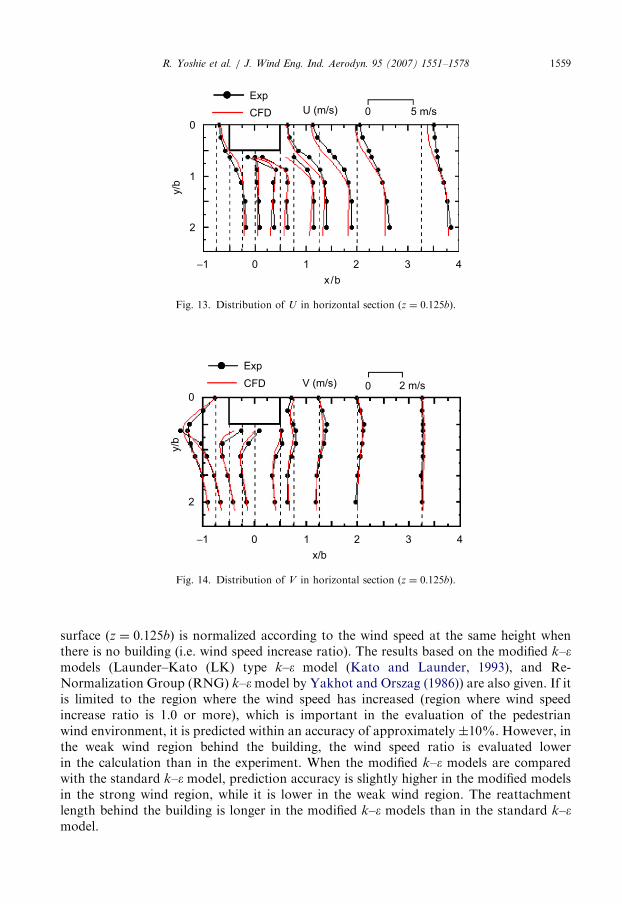
(2) Wind velocity distribution on a horizontal cross-section: The distributions of U and V

on the horizontal plane ðz=b ¼ 0:125Þ near the ground surface are shown in Figs. 13and 14, respectively. The calculated values and the experimental values agree relatively well

ARTICLE IN PRESS

4

3

2

1

0

−1 0 1

x /b

2 3 4

z/b

Exp

CFD W (m/s) 0 2 m/s

Fig. 12. Distribution of W in vertical section ðy ¼ 0Þ.

Exp

CFD U (m/s) 0 5 m/s

4

3

2

1

0

z/b

−1 0 1

x/b

2 3 4

Fig. 11. Distribution of U in vertical section ðy ¼ 0Þ.


except that the calculated U is lower than the experimental value in the wake region. Thereattachment length behind the building is longer in the calculation.(3) Wind speed increase ratios near the ground surface: Fig. 15 compares the experimental

and calculated scalar wind velocity. The scalar wind velocity (wind speed) near the ground

ARTICLE IN PRESS

0

1

2

−1 0 1 2 3 4

x/b

y/b

Exp

CFD V (m/s) 0 2 m/s

Fig. 14. Distribution of V in horizontal section ðz ¼ 0:125bÞ.

0

1

2

−1 0 1 2 3 4

x/b

Exp

CFD U (m/s) 0 5 m/s

y/b

Fig. 13. Distribution of U in horizontal section ðz ¼ 0:125bÞ.


surface ðz ¼ 0:125bÞ is normalized according to the wind speed at the same height whenthere is no building (i.e. wind speed increase ratio). The results based on the modified k–�models (Launder–Kato (LK) type k–� model (Kato and Launder, 1993), and Re-Normalization Group (RNG) k–�model by Yakhot and Orszag (1986)) are also given. If itis limited to the region where the wind speed has increased (region where wind speedincrease ratio is 1.0 or more), which is important in the evaluation of the pedestrianwind environment, it is predicted within an accuracy of approximately �10%. However, inthe weak wind region behind the building, the wind speed ratio is evaluated lowerin the calculation than in the experiment. When the modified k–� models are comparedwith the standard k–� model, prediction accuracy is slightly higher in the modified modelsin the strong wind region, while it is lower in the weak wind region. The reattachmentlength behind the building is longer in the modified k–� models than in the standard k–�model.

ARTICLE IN PRESS

1.6

1.4

1.2

1

0.8

0.6

0.4

0.4 0.6 0.8 1 1.2 1.61.4

0.2

0.20

0

Experiment

0.4 0.6 0.8 1 1.2 1.61.40.20

Experiment

0.4 0.6 0.8 1 1.2 1.61.40.20

Experiment

Calc

ula

tion

1.6

1.4

1.2

1

0.8

0.6

0.4

0.2

0

Calc

ula

tion

1.6

1.4

1.2

1

0.8

0.6

0.4

0.2

0

Calc

ula

tion

x/b = -0.75

x/b = -0.5

x/b = -0.25

x/b = 0x/b = 0.5

x/b = 0.75x/b = 1.25

x/b = 2

x/b = 3.25

± 0%

± 1 0%

In front of building

Side of building

Behind building

Standard

k-ε model

LK k-εmodel

RNG k-εmodel

Fig. 15. Wind speed increase ratio near floor ðz ¼ 0:125bÞ.


3.4. Influence of various calculation conditions on the calculated results

Here, the results obtained by changing the calculation conditions are summarizedwithout diagrams. Furthermore, the findings obtained from the benchmark test on the flowfield around a square prism of 4:4:1 (Fig. 2) are also given. Detailed information on thestudies is in the following references; Working Group for CFD Prediction of WindEnvironment Around Building (2001), Mochida et al. (2002); Shirasawa et al. (2003) andTominaga et al. (2003, 2004).(1) When the modified k–� models were used, a reverse flow on the roof was reproduced,

and the prediction accuracy in the strong wind region near the separation region closer tothe ground surface was improved. However, in the region behind the building, thereattachment length was longer than for the standard k–� model, and agreement with theexperimental results deteriorated.

ARTICLE IN PRESSR. Yoshie et al. / J. Wind Eng. Ind. Aerodyn. 95 (2007) 1551–1578 1561

(2) When LES was performed, the prediction accuracy in the flow field behind thebuilding was dramatically improved. This is mainly because the periodic vortex sheddingbehind the square prism was well reproduced by LES (Tominaga et al., 2003).

(3) When the calculation was conducted on a finer grid (by decreasing the grid width ofthe standard calculation grid to 1

2), the results were very close to those for the standard

grid. Thus, the grid arrangement of the standard condition was sufficient.(4) When the standard computational domain ð21b� 13:75b� 11:25bÞ was narrowed

down to a small region ð13:8b� 7:56b� 7:75bÞ, there was almost no change in the results.(5) When k and � in the inflow were varied, the calculated results varied widely. Thus, it

is important to provide appropriate values for inflow k and �.(6) When a first-order upwind scheme was used for the advection term, the velocity

distribution at the side region of the building, where wind enters the computational gridsdiagonally, become less steep. This is not desirable.

(7) Comparative studies performed by unifying the calculation conditions showedsmall differences between the calculated results for three commercial codes and two self-made codes.

4. Flow field around a high rise-building located in a city

This chapter describes the results of the study on the flow field near a high-rise buildingin a typical (regular) urban block.

4.1. General features of the wind tunnel experiment

The flow field analyzed here is that around a high-rise building in a simple urban area,for which the wind tunnel experiment was carried at the Niigata Institute of Technology.The low-rise urban block was assumed to be 40m square and 10m high as shown in Fig. 16(simulating a condition where low-rise houses are densely packed), with a high-risebuilding 25m square and 100m high (1:1:4) in a block at the center of this area. One urbanblock is assumed to be enclosed by two roads (each 10m wide) and roads 20 and 30mwide. This is one of the typical Japanese situations where a high-rise condominium is built.

Wind direction0°

22.5°

45°

10m road

10m road

30m road

20m road

Fig. 16. General features of wind tunnel experiment.

ARTICLE IN PRESS

40m

10m

10m

40m 40m20m 30m

Experiment

Scale: 1/400

Measuring height :5 mm

0°

45°

Fig. 17. Measuring points.

Table 2

Standard calculation conditions

Computational domain 1:8m� 1:8m� 1:8m(the size of the test section of the wind tunnel)

Grid resolution 132 ðxÞ � 130 ðyÞ � 76 ðzÞ ¼ 1; 304; 160 mesh (Fig. 18)

Scheme for advection term Quick scheme for U , V , W , k, �Building wall and ground surface Logarithmic law for smooth surface wall

Upper and side surface of computational domain Free slip wall condition (symmetric plane)

Turbulence model Standard k–� model

Inflow boundary condition Interpolated values of U and k from

the experimental approaching flow

� ¼ C1=2m k � dU=dz ð� ¼ PkÞ, Cm ¼ 0:09



The wind velocity measuring points are shown in Fig. 17. The scale of the experimentalmodel was 1

400and the measuring height was 5mm above the floor of the wind tunnel (2m

above ground in real scale). Wind velocity was measured in three wind directions (0�, 22:5�

and 45�) using a thermister anemometer. In addition, for wind direction 0� only, the windvelocity was measured using a split film probe. The inflow wind velocity UH at the heightof the central high-rise building H (H ¼ 250mm in the experiment and 100m in real scale)was 6:6m=s.

4.2. General outline of calculation

The problems with the CFD analysis on the urban area, as described above, are: (1)How wide should the computational domain be maintained in the horizontal and verticaldirections? (2) How fine should the grid resolution be? (3) To what extent should thesurrounding urban blocks be reproduced? (4) What model should be used as a turbulenceclosure? Based on the standard calculation conditions shown in Table 2 and Fig. 18, theprediction accuracy of CFD simulation was examined. By varying the calculation

ARTICLE IN PRESS

x

y

1.8m

1.8

m

High-rise building

was divided into

12(x) 12(y) 27(z)

a

b

Fig. 18. Computational domain and grid resolution for standard calculation condition. (a) Whole computational

domain and grid resolution. (b) Macrograph of central area.


conditions of (1)–(4), the influences of the calculation conditions on the CFD results wereinvestigated.

4.3. Comparison of CFD results with experimental results based on standard calculation

conditions

The calculated results based on the standard calculation conditions and the experimentalresults are compared in Fig. 19(a) (wind direction 0�) and in Fig. 19(b) (wind direction45�). (In these figures, experimental data at measuring points very close to the high-risebuilding (points 26–29 and 40–43) were omitted because their reliability was considered tobe low.) The wind speed ratio between the scalar wind velocity and UH at the measuringpoint is represented on the ordinate. At measuring points 35, 38 where the wind velocitywas highest for wind directions 0� and 45�, the calculated results were about 15% lower

ARTICLE IN PRESS

1

0.8

0.6

0.4

0.2

0

Win

d S

peed R

atio

1

0.8

0.6

0.4

0.2

0

Win

d S

peed R

atio

0 5 10 15 20 25 30 35 40 45 50 55 60 65 70 75

0 5 10 15 20 25 30 35 40 45 50 55 60 65 70 75

Measuring Point No.

Measuring Point No.

CFD

Exp.

CFD

Exp

Fig. 19. Comparison between CFD based on standard calculation conditions and experiment. (a) Wind

direction ¼ 0. (b) Wind direction ¼ 45�.

0.8

0.6

0.4

0.2

0Win

d S

peed R

atio

0 5 10 15 20 25 30 35 40 45 50 55 60 65 70 75

Measuring Point No.

Small(1.5m×1.5m)

Standard(1.8m×1.8m)

Larqe(3.6m×3,6m)

Fig. 20. Influence of horizontal computational domain.


than the experimental results, while relatively good matching was observed for the otherstrong wind regions.

4.4. Influence of various calculation conditions on CFD results

(1) Influence of size of horizontal computational domain: The calculation was carried outin experimental scale. To evaluate the influence of the horizontal computational domain, itwas expanded from the standard domain of 1:8m� 1:8m to one of 3:6m� 3:6m, andcontracted to one of 1:5m� 1:5m, which is near the rim of the surrounding block. Theresults are shown in Fig. 20. When the horizontal computational domain was largeð3:6m� 3:6mÞ, the wind speed tended to decrease slightly with the decrease of theobstruction ratio in the horizontal direction. On the other hand, when the calculation was

ARTICLE IN PRESS

0.8

0.6

0.4

0.2

0Win

d S

peed R

atio

0 5 10 15 20 25 30 35 40 45 50 55 60 65 70 75

Measuring Point No.

Standard mesh

Coarse mesh

Fine mesh

Fig. 22. Influence of grid width.

0.8

0.6

0.4

0.2

0

Win

d S

peed R

atio

0 5 10 15 20 25 30 35 40 45 50 55 60 65 70 75

Measuring Point No.

Low(2H)

Middle(3H)

Standard(7.2H)

Fig. 21. Influence of vertical computational domain.


carried out in the smaller domain ð1:5m� 1:5mÞ, the wind speed became higher. Thehorizontal computational domain has a considerable influence on the results. It issomewhat difficult to interpret this result to real situation. We think if the similar urbanarea is spread outside of the computational domain, side space of the computationaldomain should be narrow. But if the outside of the urban area is open terrain, thecomputational domain should be large.

(2) Influence of vertical computational domain: Fig. 21 shows the results obtained whenthe vertical computational domain was lowered from the standard height of 7:2H to 3H

and 2H. When the upper computational domain was 2H, the wind speed was just slightlyhigher. There was almost no difference between the cases of 7:2H and 3H. It appears thatno substantial problem occurred even when the vertical computational domain waslowered to about 3H.

(3) Influence of grid resolution: Fig. 22 shows the calculated results when a fine grid and acoarse grid were used. For the fine grid (215ðxÞ � 202ðyÞ � 101ðzÞ ¼ 4; 386; 430 grids), thegrid width was set to about 1

1:5 of the standard grid in all three directions x, y and z. For thecoarse grid (74ðxÞ � 68ðyÞ � 48ðzÞ ¼ 241; 536 grids), it was about 1.5 times the standardgrid. The difference between the calculated results for the standard grid and the fine gridwas very small. The difference between the calculated results for the coarse grid and theother cases was also small. The standard grid would be satisfactory, i.e. with each side ofthe high-rise building divided into 10 portions or more.

(4) Influence of reproduction range of surrounding urban blocks: Fig. 24 shows the resultsof calculation with two rows and three rows each deleted from the peripheral region of the

ARTICLE IN PRESS

0.8

0.6

0.4

0.2

0

Win

d S

peed R

atio

0 5 10 15 20 25 30 35 40 45 50 55 60 65 70 75

Measuring Point No.

Standard

Deleting 2 rows

Deleting 3 rows

Fig. 24. Influence of reproduction range of surrounding urban blocks.

1

0.8

0.6

0.4

0.2

0

Win

d S

peed R

atio

0 5 10 15 20 25 30 35 40 45 50 55 60 65 70 75

Measuring Point No.

Standard k-εRNG k-εExp.

Fig. 25. Influences of deferent turbulence models.

Fig. 23. Reproduction range of surrounding urban blocks. (a) Deleting 2 rows. (b) Deleting 3 rows.


surrounding urban blocks, as shown in Fig. 23. The difference from the standard case wasvery small except at measuring points 1, 2, 3 and 4 on the roads on the windward side.Therefore, the reproduction range of the surrounding urban blocks would be satisfactoryfor practical application if at least one block was maintained in the surroundings of theregion to be evaluated (Figs. 23 and 24).(5) Influence of modification on turbulence modelling: Fig. 25 shows calculated results

based on the modified k–� model (RNG k–� model). At measuring points 35, 38, etc.,


where the wind speed was high, the results from the modified k–� model was higher thanthat of the standard k–� model, and matching with the experimental results was improved.However, in the weak wind regions such as at measuring points 15–25, where the windspeed was low, matching with the experimental results deteriorated.

4.5. Summary

According to the results of the present study, the influence on the calculated results ofthe computational domain, the grid resolution, and the reproduction range of thesurrounding urban block was relatively low. In the calculation for practical applications,the criteria would be as follows: at least one urban block of several tens of metersshould be reproduced in the area surrounding the region to be evaluated, and the upperspace region should be maintained at 3H or more, and each side of the high-rise buildingshould be divided into 10 portions or more. And when the similar urban block isspread outside of the computational domain, side space of the computational domainshould be narrow, but when the outside of the urban area is open terrain, thecomputational domain should be large. If it is limited to the highest wind region, whichis important for evaluation of the pedestrian wind environment around the building, thewind speed difference between CFD and experiment was about 15% at most forthe standard k–� model. For the RNG model, more accurate prediction can be made in thestrong wind region.

5. Flow field in an actual urban area (Niigata)

Up to this point, we have reported results of bench mark tests for relativelysimple shapes such as single buildings and relatively regular model urban blocks. Inactual urban areas, however, buildings have complicated shapes and are distributedin an irregular manner. In order to accurately reproduce them in a CFD simulation,a great number of grids are required. In particular, when an orthogonal structured gridsystem is used, it is difficult to provide a grid configuration that matches well withthe building configuration, and special care must be taken to allow for the influenceof mismatching on the prediction accuracy. This problem can be solved if anunstructured grid system is used, although there are some difficulties in preparing thiskind of grid.

Furthermore, for the wind environment in urban areas, prediction is normally made for16 wind directions on two patterns, i.e. before and after the construction of the proposedbuilding. In some situations, it is necessary to consider protection against wind such asplanting trees. This increases the number of cases that need to be considered, andcalculation accuracy must be maintained under restrictive conditions for practicalapplication.

This chapter describes a study in an actual urban area in Niigata, where low-rise housesare packed closely together. Wind tunnel experiments and CFD simulation wereperformed to predict the wind speed distribution and to assess the pedestrian windenvironment, and the results were compared. Furthermore, the differences are shownbetween three types of grid system: a single structured grid system (orthogonal mesh), anoverlapping structured grid system, and an unstructured grid system (Tominaga et al.,2004).

ARTICLE IN PRESS

Fig. 26. Actual urban model (CAD data) and measuring points.

Table 3

Common calculation conditions specified

Inflow boundary Interpolated values of U and k from the experimental

approaching flow. � ¼ CD1=2 � k � dU=dz � ¼ PkÞ

Computational domain Area about 500m ðxÞ � 500m ðyÞ � 300m ðzÞ that includes

the whole urban block

Upper surface of computational domain Free slip wall condition (symmetric plane)


Ground surface boundary Logarithmic law with roughness length z0 ðz0 ¼ 0:024mÞBuilding surface boundary Logarithmic law for smooth wall


5.1. Urban area model under study and outline of wind tunnel experiment

The study was performed on an urban area model. This model consisted of an actual cityblock in Niigata city, Niigata prefecture, Japan with low-rise houses packed closelytogether. A target building 60m high (Building A) and two target buildings 18m high(Buildings B and C) were assumed to be constructed 26 (Fig. 26). Wind tunnel experimentsat 1

250scale were performed on this model in a turbulent boundary layer with a power law

exponent of 0.25. Scalar wind velocities at 8mm above the wind tunnel floor (2m abovethe ground surface in real scale) were measured by multi-point thermister anemometers.

5.2. Outline of numerical calculation

The items shown in Table 3 were specified as common calculation conditions in thecomparative study. For the configuration of the urban block, input data for each CFDcode were prepared from the same CAD data obtained from the drawing of the windtunnel model. The features of the compared CFD codes and the different calculation

ARTICLE IN PRESS

Table 4

Outline of CFD codes and calculation conditions

CFD Code (1) Computational method and time

integral scheme.

Grid arrangements

(2) Turbulence model.

(3) Scheme for advection term.

Code O (Self-made code) (1) Overlapping structured grid, artifical

compressibility.

(2) Standard k2�.(3) Third-order upwind.

Code M (Commerical code:

STREAM for Windows)

(1) Structured gird, SIMPLE, steady

state.

(2) Standard k2�.(3) QUIK.

Code T (Commerical code:

SCRYU/Tetra for Windows)

(1) Unstructured grid, SIMPLE, steady

state.

(2) Standard k2�.(3) MUSCL(2nd-order).


conditions are summarized in Table 4, as well as general features of the grid systems usedin each CFD code.

5.3. Results of numerical analysis

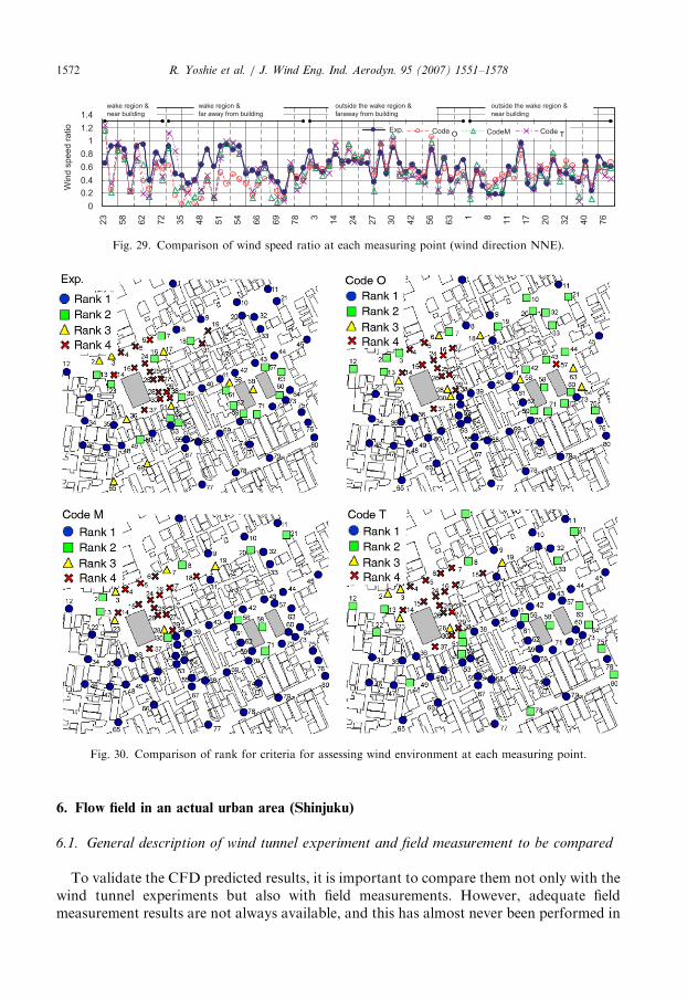
(1) Comparison based on wind speed ratio: CFD simulations were conducted for 16 winddirections. Here, predicted results and experimental results of the wind speed ratio arecompared for the wind direction NNE, which is the wind direction most frequentlyoccurring in Niigata. The wind speed ratio is the ratio of wind speed (scalar velocity) ateach measuring point ðheight ¼ 2mÞ and the wind speed at the same height at the inflowboundary. There was no substantial difference among codes for overall distribution ofwind speed ratio. As a representative example, the distribution of wind speed ratio basedon CFD code T (Table 4) is shown in Fig. 27. Regions with very high wind speed were

ARTICLE IN PRESS

Fig. 27. Distribution of wind speed ratio near ground surface ðz ¼ 2mÞ (Code T) (blue line indicates the wake

region).


found at the corners on the northwest and east sides of Building A. Furthermore, strongwind caused by contraction flow was seen between Buildings B and C.Fig. 28 represents the correlation of wind speed ratio obtained from CFD codes with the

results of wind tunnel experiments. Plotting is shown separately inside and outside thewake region of the target buildings (The wake region is indicated in Fig. 27). The predictedresults in the CFD codes were almost identical, and there was no clear difference amongthe codes. In the wake region of the target buildings, there was a tendency to underestimatethe wind speed compared with the results of the wind tunnel experiment, while in otherregions the matching was relatively satisfactory. The CFD results often tended tounderestimate the wind speed in the wake region of the building in benchmark tests onother configurations.Fig. 29 compares the wind speed ratios at each measuring point. For the positions of the

measuring points, see Fig. 26. The CFD results generally agree well with the results of thewind tunnel experiment. In particular, the prediction accuracy is high ‘‘outside the wakeregion & near building’’. The difference from experimental results was large at severalmeasuring points, but these were mostly in alleys in the wake region of the target buildings.This may be because a slight difference in the prediction of the separation shear layer dueto the difference in reproducibility of the building configuration may have influenced thecalculated results, and because there were shape errors in the actual wind tunnel model andCAD data used, and also errors in the positions of the evaluation point.(2) Comparison based on criteria for assessing wind environment: A rank evaluation was

performed on the CFD predicted results according to criteria for assessing the windenvironment proposed by Murakami et al. (1986). This was based on the occurrencefrequency of daily maximum gust wind speed using observation data from the NiigataRegional Meteorological Observatory. The results are summarized in Fig. 30. The gustfactor GF was assumed to be 2.5 to convert the calculated average wind speeds to themaximum gust wind speeds. Including the results at the measuring points with rank 4 onthe northeast and south sides of Building A, the CFD results generally showed good

ARTICLE IN PRESS

1.4

1.2

0.8

0.6

0.4

0.2

0

1

CF

D

0.2 0.4 0.6 0.8 1 1.2 1.40

Experiment

1.4

1.2

0.8

0.6

0.4

0.2

0.2 0.4 0.6 0.8 1 1.2 1.4

0

0

1

CF

D

Experiment

1.4

1.2

0.8

0.6

0.4

0.2

0

1

CF

D

0.2 0.4 0.6 0.8 1 1.2 1.40

Experiment

Fig. 28. Correlation of wind speed ratio between CFD result and experimental result (wind direction NNE): (a)

Code O; (b) Code M; (c) Code T.


matching with the wind tunnel experiment results. However, as described above, there weredifferences between some of the experimental results and CFD codes for the measuringpoints near low-rise houses in alleys or along large avenues.

ARTICLE IN PRESS

0

0.2

0.4

0.6

0.8

1

1.2

1.4

23

58

62

72

35

48

51

54

66

69

78 3

14

24

27

30

42

56

63 1 8

11

17

20

32

40

76

Exp. Code O CodeM Code T

Win

d s

peed r

atio

Fig. 29. Comparison of wind speed ratio at each measuring point (wind direction NNE).

Fig. 30. Comparison of rank for criteria for assessing wind environment at each measuring point.


6. Flow field in an actual urban area (Shinjuku)

6.1. General description of wind tunnel experiment and field measurement to be compared

To validate the CFD predicted results, it is important to compare them not only with thewind tunnel experiments but also with field measurements. However, adequate fieldmeasurement results are not always available, and this has almost never been performed in

ARTICLE IN PRESS

Fig. 31. Urban area reproduced and measuring points.


the past. Thus, a benchmark test was conducted on the Shinjuku Sub-central Area inTokyo, Japan in its early development stage, for which detailed wind tunnel experimentsand field measurements had been carried out in cooperation with many researchorganizations during construction (Yoshida et al., 1978; Asami et al., 1978). Using thesedata, the validity of the prediction accuracy of CFD was assessed.

(1) Wind tunnel experiment: A number of wind tunnel experiments had been performedon the Shinjuku Sub-central Area. Here, the CFD simulations were carried out based onthe condition of the 1977 Experiment.

(2) Field measurements: Field measurements were carried out from December 1975 toNovember 1983. The present CFD simulations were performed for conditions in 1977when the situation of field measurements was similar to those of the wind tunnelexperiment model. In the field measurements, three-cup anemometers were used. Themeasurement heights differed according to the measuring point, being 3–9m above theground surface. The reproduced urban area and the measuring point distribution areshown in Fig. 31. Measured wind speeds at encircled points (Nos. 6, 7, 13, 15) werecompared with the calculated ones.

6.2. Outline of numerical calculations

As for the study on the urban area of Niigata City, common calculation items weredesignated. For the configuration of urban blocks, no wind tunnel experiment models atthe time of measurement were remained. Thus, we made CAD data of the urban areaconfiguration and topography based on the old drawings, photographs, and white maps in1977. Because no details on the topographical height difference were available, the

ARTICLE IN PRESS

Fig. 32. CAD data of urban area.

Fig. 33. Grid arrangements of CFD codes: (a) CFD_A (Self made code); (b) CFD_B (SCRYU/Tetra for

Windows); (c) CFD_C (Fluent).


reproduction was made stepwise every 5m by referring to the maps in 1977. The CAD datathus prepared are shown in Fig. 32. Fig. 33 shows the grid arrangements of the CFD codes.Here, only CFD_A uses a structured grid system, while the others are based on a non-structured grid. However, CFD_A uses an overlapping grid.

6.3. Comparison of CFD results with wind tunnel experiment results and field measurements

Similar to the wind tunnel experiment and the field measurements, the wind speedobtained by CFD was normalized by the wind speed at reference points. The referencepoints were the top of the Shinjuku Mitsui Building (D in Fig. 31; height of observation

ARTICLE IN PRESS

Wind direction at reference point

Win

d s

pe

ed

ra

tio No. 6

Win

d s

pe

ed

ra

tio


No. 7

Win

d s

pe

ed

ra

tio


No.13

Win

d s

pe

ed

ra

tio

No. 15


1.0

0.5

0.0

1.0

0.5

0.0

1.0

0.5

0.0

1.0

0.5

0.0

NE E SE S SW W NW N

NE E SE S SW W NW N

NE E SE S SW W NW N

NE E SE S SW W NW N

Fig. 34. Comparison of wind speed ratio for 16 wind directions.


ARTICLE IN PRESS

1

0.8

0.6

0.4

0.2

0

Norm

aliz

ed V

elo

city

23 27 28 29 36 14 26 7 33 13 15

Measuring Point

field meas. (mean)

field meas. (+σ)

field meas. (-σ)

wind tunnel

CFD_A

CFD_B

CFD_C

Fig. 35. Comparison of wind speed ratio at each measuring point with wind direction S.


237m) for the wind directions NE–N–NW, and the top of the KDD Building (C in Fig. 31;height of observation 187m) for the other wind directions. The measurement values forreference wind speeds of 5 m/s or more were extracted from the observation data in theyear 1977, and the average value of normalized wind speed for each wind direction wasused as the measurement value.Fig. 34 compares the experimental results and the field measurements for wind speed

ratios (normalized wind speeds) at representative measuring points. As a general trend, thewind tunnel experiment results are within the standard deviation of the field measurements,and the CFD results are also generally within the same range. The difference amongcalculation results is relatively small regardless of the code and the grid system.But the CFD results deviate from the experiment results and field measurements

depending on the measuring point and wind direction as follows.

(1)
Measuring point 7, wind direction E: Calculated wind speed is higher than the measuredone. Measuring point 7 is located in the contracted flow region when the wind directionis E. As mentioned above, the reproduction accuracy of the CAD data was notnecessarily sufficient. The small difference in position between CFD and measurementmight cause large difference in wind speeds between them in this contracted flow region.
(2)
Measurment point 13, wind direction SSW– WSW: Calculated wind speeds are lowerthan the measured ones. For these wind direction, the measuring point 13 is located inwake region of the high-rise buildings. This underestimation in wake region is commonto that for the case of the 2:1:1 square prism and for the case of the actual urban area inNiigata.
(3)
Measurment point 15, wind direction NE: The measured wind speeds largely changefrom wind direction NE to ENE, while the calculated ones largely change from NNEto NE. The small deference in reference wind directions between measurement andCFD might bring large difference in wind speeds.
Next, Fig. 35 compares the wind speed ratios at the measuring points with wind directionS. In general, the difference among the results of the three CFD codes is small, and theCFD results showed good matching with the experimental results and field measurements


except at nos. 27, 28, 29, 36. These measuring points are located near the boundary of thecomputational domain. We should have taken the horizontal computational domainlarger, and should have reproduced more urban blocks around these measuring points forthe better prediction.

7. Conclusion—current status and problems in CFD prediction

This paper has described some results of a study by the ‘‘Working Group forPreparation of Wind Environment Evaluation Guideline based on CFD’’.

In general, prediction accuracy for the weak wind regions behind buildings was notsatisfactory, while prediction accuracy for the strong wind region was fairly high. In singlebuilding models, which are considered to give the highest accuracy in the experiment, theCFD analysis results were consistent with experimental results within an accuracy about 10%in the strong wind region. However calculated U was lower than the experimental value inthe wake region behind the building. The reattachment length behind the building was longerin the calculation. For the urban block model, which is considered to give the next mostaccurate results in the experiment, the CFD analysis results in strong wind regions showed aprediction accuracy within 10 or so % for the standard k–� model and better accuracy for themodified k–� models. In actual urban area models, the CAD data for CFD simulation didnot completely match with experiment and field measurements, and it is difficult toquantitatively describe the prediction accuracy. However, relatively good matching wasfound in the strong wind region. The reason why the CFD analysis results underestimate thewind velocity in the wake regions may be because it is not possible to reproduce the vortexshedding in RANS type models such as the k–� model. In LES, this can be improved, and themaximum instantaneous wind velocity can also be evaluated in LES. However, in order touse LES in general-purpose applications for predicting the wind environment aroundbuildings, we need a dramatic increase in computer processing speed in the future. For thetime being, we must be content with RANS type models currently in use. In RANS typemodels, it is only possible to evaluate average wind velocity. To evaluate pedestrian windenvironment based on maximum gust wind speed we need to convert from average windspeed to maximum gust wind speed based on the assumption of the gust factor.

Although there are problems as described above in the CFD analysis using the RANStype turbulence models, it is advantageous that the detailed and overall spatial distributionof wind velocity can be identified in CFD analysis, while only limited information on windvelocity can be obtained from wind tunnel experiments. Strong wind points that may havebeen missed in wind tunnel experiments may be identified by the CFD simulation. Further,there are some uncertainties inherent in wind tunnel experiments (such as measuringinstrument errors, incidental errors, errors in the position where the sensor is installed,etc.), but there are no such uncertainties in CFD. Furthermore, it is very difficult to havean arbitrary approach flow in the wind tunnel, while this can be freely done in CFD. It thusappears possible to reduce the differences in prediction accuracy between wind tunnelexperiment and CFD on practical assessment.

Acknowledgment

The authors would like to express their gratitude to the members of the ‘‘WorkingGroup for Preparation of Wind Environment Evaluation Guideline based on CFD’’. Note:

ARTICLE IN PRESSR. Yoshie et al. / J. Wind Eng. Ind. Aerodyn. 95 (2007) 1551–15781578

The working group members are: A. Mochida (Chair, Tohoku Univ.), Y. Tominaga(Secretary, Niigata Inst. of Tech.), Y Ishida (Kajima Corp.), T. Ishihara (Univ. of Tokyo),K. Uehara (National Inst. of Environ. Studies), R. Ooka (I.I.S., Univ. of Tokyo),H. Kataoka (Obayashi Corp.), T. Kurabuchi (Tokyo Univ. of Sci.), N. Kobayashi (Tokyopolytechnic Univ.), N. Tuchiya (Takenaka Corp.), Y. Nonomura (Fujita Corp.), T. Nozu(Shimizu Corp.), K. Harimoto (Taisei Corp.), K. Hibi (Shimizu Corp.), S. Murakami(Keio Univ.), R. Yoshie (Tokyo Polytechnic Univ.).

References

Asami, Y., Iwasa, Y., Fukao, Y., Kawaguchi, A., Yoshida, M., Sanada, S., Fujii, K., and Members of AIJ, 1978.

Full-scale measurement of environmental wind on New-Shinjuku-Center—characteristics of wind in built-up

area (part 2). In: Proceeding of Fifth Symposium on Wind Effects on Structures, pp. 83–90.

Franke, J., Hirsch, C., Jensen A.G., Krus, H.W., Schatzmann, M., Westbury, P.S., Miles, S.D., Wisse, J.A.,

Wright, N.G., 2004. Recommendations on the use of CFD in predicting pedestrian wind environment, COST

Action C14 ‘‘Impact of Wind and Storms on City Life and Built Environment’’.

Kato, M., Launder, B.E., 1993. The modelling of turbulent flow around stationary and vibrating square cylinders.

In: Nineth Symposium on Turbulent Shear Flows, pp. 10–14.

Meng, Y., Hibi, K., 1998. Turbulent measurements of the flow field around a high-rise building. J. Wind Eng. Jpn.

(76), 55–64.

Mochida, A., Tominaga, Y., Murakami, S., Yoshie, R., Ishihara, T., Ooka, R., 2002. Comparison of k–� models

and DSM applied to flow around a high-rise building—report on AIJ cooperative project for CFD prediction

on wind environment. Wind Struct. 5 (2–4), 227–244.

Murakami, S., Iwasa, Y., Morikawa, Y., 1986. Study on acceptable criteria for assessing wind environment at

ground level based on residents’ diaries. J. Wind Eng. Ind. Aerodyn. 24 (1), 1–18.

Shirasawa, T., Mochida, A., Tominaga, Y., Yoshie, R., Kataoka, H., Nozu T., Yoshino, H., 2003. Development

of CFD method for predicting wind environment around a high-rise building, Part 2: the cross comparison of

CFD results on the flow field around a 4:4:1 prism. AIJ J. Technol. Des. (18), 441–446.

Tominaga, Y., Mochida, A., Murakami, S., 2003. Large eddy simulation of flowfield around a high-rise building.

In: 11th International Conference on Wind engineering, B10-5.

Tominaga, Y., Mochida, A., Shirasawa, T., Yoshie, R., Kataoka, H., Harimoto, K., Nozu, T., 2004. Cross

comparisons of CFD results of wind environment at pedestrian level around a high-rise building and within a

building complex. J. Asian Archit. Build. Eng. 3 (1), 63–70.

Tominagada, Y., Mochida, A., Harimoto, K., Kataoka, H., Yoshie, R., 2004. Development of CFD method for

predicting wind environment around a high-rise building, Part 3: the cross comparison of results for wind

environment around building complex in actual urban area using different CFD codes. AIJ J. Technol. Des.

(19), 181–184.

Working Group for CFD Prediction of Wind Environment Around Building, 2001. Development of CFDmethod

for predicting wind environment around a high-rise building, Part 1: the cross comparison of CFD results

using various k–� models. AIJ J. Technol. Des. (12), 119–124.

Yakhot, V., Orszag, S.A., 1986. Renormalization goup analysis of turbulence. J. Sci. Comput. 1 (1), 3–51.

Yoshida, M., Sanada, S., Fujii, K., Asami, Y., Iwasa, Y., Fukao, Y., Kawaguchi, A., and Members of AIJ, 1978.

Full-scale measurement of environmental wind on New-Shinjuku-Center—characteristics of wind in built-up

area (part 1). In: Proceeding of Fifth Symposium on Wind Effects on Structures, pp. 75–82.

Documents

Cooperative project for CFD prediction of pedestrian … · and Industrial Aerodynamics 95 (2007) 1551–1578 Cooperative project for CFD prediction of pedestrian wind environment