Cooperative Inverse Reinforcement Learning

Dylan Hadfield-Menell Anca Dragan Pieter Abbeel Stuart RussellElectrical Engineering and Computer Science

University of California at BerkeleyBerkeley, CA 94709

Abstract

For an autonomous system to be helpful to humans and to pose no unwarrantedrisks, it needs to align its values with those of the humans in its environment insuch a way that its actions contribute to the maximization of value for the humans.We propose a formal definition of the value alignment problem as cooperativeinverse reinforcement learning (CIRL). A CIRL problem is a cooperative, partial-information game with two agents, human and robot; both are rewarded accordingto the human’s reward function, but the robot does not initially know what thisis. In contrast to classical IRL, where the human is assumed to act optimally inisolation, optimal CIRL solutions produce behaviors such as active teaching, activelearning, and communicative actions that are more effective in achieving valuealignment. We show that computing optimal joint policies in CIRL games can bereduced to solving a POMDP, prove that optimality in isolation is suboptimal inCIRL, and derive an approximate CIRL algorithm.

1 Introduction

“If we use, to achieve our purposes, a mechanical agency with whose operation we cannot interfereeffectively . . . we had better be quite sure that the purpose put into the machine is the purpose whichwe really desire.” So wrote Norbert Wiener (1960) in one of the earliest explanations of the problemsthat arise when autonomous systems operate with objectives that differ from those of humans. Thisvalue alignment problem is not trivial to solve. Humans are prone to mis-stating their objectives,which can lead to unexpected implementations, as King Midas found out. Russell & Norvig (2010)give the example of specifying a reward function for a vacuum robot: if we reward the action ofcleaning up dirt, which seems reasonable, the robot repeatedly dumps and cleans up the same dirt tomaximize its reward.A solution to the value alignment problem has long-term implications for the future of AI and itsrelationship to humanity (Bostrom, 2014) and short-term utility for the design of usable AI systems.Giving robots the right objectives and enabling them to make the right trade-offs is crucial forself-driving cars, personal assistants, and human–robot interaction more broadly. Value alignmentproblems are not unique to artificial systems. Economic systems often involve multiple agents withdistinct objectives (e.g., employees and employers) and for whom incentive schemes (e.g., wages)must be designed. Kerr (1975) explains several examples of value misalignment in this context. Ourwork has strong connections with the principal–agent problem from economics; we give a briefoverview in Section 2.The field of inverse reinforcement learning or IRL (Russell, 1998; Ng & Russell, 2000; Abbeel& Ng, 2004) is certainly relevant to the value alignment problem. An IRL algorithm infers thereward function of an agent from observations of the agent’s behavior, which is assumed to beoptimal (or approximately so). One might imagine that IRL provides a simple solution to the valuealignment problem: the robot observes human behavior, learns the human reward function, andbehaves according to that function. This simple idea has two flaws. The first flaw is obvious: wedon’t want the robot to adopt the human reward function as its own. For example, human behavior(especially in the morning) often conveys a desire for coffee, and the robot can learn this with IRL,

arX

iv:1

606.

0313

7v2

[cs

.AI]

5 J

ul 2

016

but we don’t want the robot to want coffee! This flaw is easily fixed: we need to formulate the valuealignment problem so that the robot always has the fixed objective of optimizing reward for thehuman, and becomes better able to do so as it learns what the human reward function is.The second flaw is less obvious, and less easy to fix. IRL assumes that observed behavior is optimalin the sense that it accomplishes a given task efficiently and this precludes a variety of useful teachingbehaviors. For example, acting optimally in coffee acquisition, while leaving the robot as a passiveobserver, is a suboptimal way to teach a robot to get coffee. Instead, the human should perhapsexplain the steps in coffee preparation and show the robot where the backup coffee supplies are keptand what do if the coffee pot is left on the heating plate too long, while the robot might ask what thebutton with the puffy steam symbol is for and try its hand at coffee making with guidance from thehuman, even if the first results are undrinkable. None of these things fit in with the standard IRLframework.Cooperative inverse reinforcement learning. We propose, therefore, that value alignment shouldbe formulated as a cooperative and interactive reward maximization process. More precisely, wedefine a cooperative inverse reinforcement learning (CIRL) problem as a two-player game of partialinformation, in which the “human”, H, knows the reward function (represented by a generalizedparameter θ), while the “robot”, R, does not; the robot’s payoff is exactly the human’s actual reward.Optimal solutions to this game maximize human reward; we show that solutions may involve activeinstruction by the human and active learning by the robot.Reduction to POMDP and Sufficient Statistics. As one might expect, the structure of CIRL gamesis such that they admit more efficient solution algorithms than are possible for general partial-information games. Let (πH, πR) be a pair of policies for human and robot, each depending, ingeneral, on the complete history of observations and actions. A policy pair yields an expected sumof rewards for each player and is a Nash equilibrium if neither actor has an incentive to deviate. InCIRL, the reward function is shared so there is well-defined optimal Nash equilibrium that maximizesvalue.1 In Section 3 we reduce the problem of computing an optimal policy pair to the solution of a(single-agent) POMDP, and hence show that the robot’s posterior over θ is a sufficient statistic, in thesense that there are optimal policy pairs in which the robot’s behavior depends only on this statistic.Moreover, the complexity of solving the POMDP is exponentially lower than the NEXP-hard boundthat (Bernstein et al., 2000) obtains for the natural reduction of the problem to a general Dec-POMDP.Apprenticeship Learning and Suboptimality of IRL-Like Solutions. In Section 3.3 we modelapprenticeship learning (Abbeel & Ng, 2004) as a two-phase CIRL game. In the first phase, thelearning phase, both H and R can take actions and this lets R learn about θ. In the second phase, thedeployment phase, R uses what it learned to maximize reward (without supervision from H). Weshow that classic IRL falls out as the best-response policy for the robot under the assumption that thehuman’s policy is “demonstration by expert” (DBE), i.e., acting optimally in isolation as if no robotexists. But we show also that this DBE/IRL policy pair is not, in general, a Nash equilibrium: even ifthe human knows the robot is running an IRL algorithm, demonstrating expert behavior is not thebest way to teach that algorithm.

Approximate Algorithm for CIRL. We introduce a graph search algorithm that approximatelycomputes H’s best response when R is running IRL and rewards are linear in θ and state features.Section 4 compares this best-response policy with the DBE policy in a grid-world example andprovides empirical confirmation that the best-response policy, which turns out to “teach” R aboutthe value landscape of the problem, is better than DBE. Thus, designers of apprenticeship learningsystems should expect that users will violate the assumption of expert demonstrations in order tobetter communicate reward.

2 Related Work

Our proposed model shares aspects with a variety of existing models. We divide the related work intothree categories: inverse reinforcement learning, optimal teaching, and principal–agent models.

Inverse Reinforcement Learning. Ng & Russell (2000) define inverse reinforcement learning(IRL) as follows: “Given measurements of an [actor]’s behavior over time. . . . Determine thereward function being optimized.” The key assumption IRL makes is that the observed behavior isoptimal in the sense that the observed trajectory maximizes the sum of rewards. We call this the

1A coordination problem arises if there are multiple optimal policy pairs; we defer this issue to future work.

2

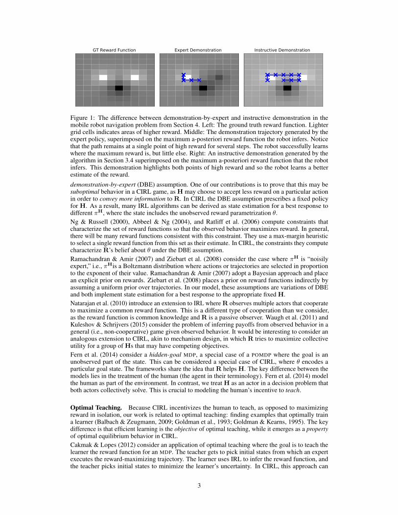
GT Reward Function Expert Demonstration Instructive Demonstration

Figure 1: The difference between demonstration-by-expert and instructive demonstration in themobile robot navigation problem from Section 4. Left: The ground truth reward function. Lightergrid cells indicates areas of higher reward. Middle: The demonstration trajectory generated by theexpert policy, superimposed on the maximum a-posteriori reward function the robot infers. Noticethat the path remains at a single point of high reward for several steps. The robot successfully learnswhere the maximum reward is, but little else. Right: An instructive demonstration generated by thealgorithm in Section 3.4 superimposed on the maximum a-posteriori reward function that the robotinfers. This demonstration highlights both points of high reward and so the robot learns a betterestimate of the reward.

demonstration-by-expert (DBE) assumption. One of our contributions is to prove that this may besuboptimal behavior in a CIRL game, as H may choose to accept less reward on a particular actionin order to convey more information to R. In CIRL the DBE assumption prescribes a fixed policyfor H. As a result, many IRL algorithms can be derived as state estimation for a best response todifferent πH, where the state includes the unobserved reward parametrization θ.Ng & Russell (2000), Abbeel & Ng (2004), and Ratliff et al. (2006) compute constraints thatcharacterize the set of reward functions so that the observed behavior maximizes reward. In general,there will be many reward functions consistent with this constraint. They use a max-margin heuristicto select a single reward function from this set as their estimate. In CIRL, the constraints they computecharacterize R’s belief about θ under the DBE assumption.Ramachandran & Amir (2007) and Ziebart et al. (2008) consider the case where πH is “noisilyexpert,” i.e., πHis a Boltzmann distribution where actions or trajectories are selected in proportionto the exponent of their value. Ramachandran & Amir (2007) adopt a Bayesian approach and placean explicit prior on rewards. Ziebart et al. (2008) places a prior on reward functions indirectly byassuming a uniform prior over trajectories. In our model, these assumptions are variations of DBEand both implement state estimation for a best response to the appropriate fixed H.Natarajan et al. (2010) introduce an extension to IRL where R observes multiple actors that cooperateto maximize a common reward function. This is a different type of cooperation than we consider,as the reward function is common knowledge and R is a passive observer. Waugh et al. (2011) andKuleshov & Schrijvers (2015) consider the problem of inferring payoffs from observed behavior in ageneral (i.e., non-cooperative) game given observed behavior. It would be interesting to consider ananalogous extension to CIRL, akin to mechanism design, in which R tries to maximize collectiveutility for a group of Hs that may have competing objectives.Fern et al. (2014) consider a hidden-goal MDP, a special case of a POMDP where the goal is anunobserved part of the state. This can be considered a special case of CIRL, where θ encodes aparticular goal state. The frameworks share the idea that R helps H. The key difference between themodels lies in the treatment of the human (the agent in their terminology). Fern et al. (2014) modelthe human as part of the environment. In contrast, we treat H as an actor in a decision problem thatboth actors collectively solve. This is crucial to modeling the human’s incentive to teach.

Optimal Teaching. Because CIRL incentivizes the human to teach, as opposed to maximizingreward in isolation, our work is related to optimal teaching: finding examples that optimally traina learner (Balbach & Zeugmann, 2009; Goldman et al., 1993; Goldman & Kearns, 1995). The keydifference is that efficient learning is the objective of optimal teaching, while it emerges as a propertyof optimal equilibrium behavior in CIRL.Cakmak & Lopes (2012) consider an application of optimal teaching where the goal is to teach thelearner the reward function for an MDP. The teacher gets to pick initial states from which an expertexecutes the reward-maximizing trajectory. The learner uses IRL to infer the reward function, andthe teacher picks initial states to minimize the learner’s uncertainty. In CIRL, this approach can

3

be characterized as an approximate algorithm for a highly restricted H that greedily minimizes theentropy of R’s belief.Beyond teaching, several models focus on taking actions that convey some underlying state, notnecessarily a reward function. Examples include finding a motion that best communicates an agent’sintention (Dragan & Srinivasa, 2013), or finding a natural language utterance that best communicatesa particular grounding (Golland et al., 2010). All of these approaches model the observer’s inferenceprocess and compute actions (motion or speech) that maximize the probability an observer infers thecorrect hypothesis or goal. Our approximate solution to CIRL is analogous to these approaches, inthat we compute actions that are informative of the correct reward function.

Principal–agent models. Value alignment problems are not intrinsic to artificial agents. Kerr(1975) describes a wide variety of misaligned incentives in the aptly titled “On the folly of rewardingA, while hoping for B.” In economics, this is known as the principal–agent problem: the principal(e.g., the employer) specifies incentives so that an agent (e.g., the employee) maximizes the principal’sprofit (Jensen & Meckling, 1976).Principal–agent models study the problem of generating appropriate incentives in a non-cooperativesetting with asymmetric information. In this setting, misalignment arises because the agents thateconomists model are people and intrinsically have their own desires. In AI, misalignment arisesentirely from the information asymmetry between the principal and the agent; if we could characterizethe correct reward function, we could program it into an artificial agent. Gibbons (1998) provides auseful survey of principal–agent models and their applications. Holmstrom & Milgrom (1987) givesstructural results on optimal incentive schemes in linear principal–agent models.From the perspective of AI research, one of the most interesting lines of research in this literaturestudies the impacts of distorted incentives. Holmstrom & Milgrom (1991) develop a multi-task modelwhere some tasks are more easily measured and rewarded than others. The key result shows thatincentives for the more precisely measured tasks should be reduced to avoid diverting too much effortfrom poorly measured tasks.

3 Cooperative Inverse Reinforcement Learning

This section formulates CIRL as a two-player Markov game with identical payoffs, proves that theproblem of computing an optimal equilibrium for a CIRL game is lower complexity than the näivebound from Dec-POMDP’s suggests, and characterizes apprenticeship learning as a subclass of CIRLgames.

3.1 CIRL Formulation

Definition 1. A cooperative inverse reinforcement learning (CIRL) game M is a two-player Markovgame with identical payoffs between a human or principal, H, and a robot or agent, R. The game isdescribed by a tuple,

M = 〈S, {AH,AR}, T (·|·, ·, ·), {Θ, R(·, ·, ·; ·)}, P0(·, ·), γ〉, (1)

with the following definitions:S a set of world states: s ∈ S.AH a set of actions for H: aH ∈ AH.AR a set of actions for R: aR ∈ AR.T (·|·, ·, ·) a conditional distribution on the next world state, given previous state and action for

both agents: T (s′|s, aH, aR).Θ a set of possible static reward parameters, only observed by H: θ ∈ Θ.R(·, ·, ·; ·) a parameterized reward function that maps world states, joint actions, and reward

parameters to real numbers. R : S ×AH ×AR ×Θ→ R.P0(·, ·) a distribution over the initial state, represented as tuples: P0(s0, θ)γ a discount factor: γ ∈ [0, 1].

We write the reward for a state–parameter pair as R(s, aH, aR; θ) to distinguish the static rewardparameters θ from the changing world state s.The game proceeds as follows. First, the initial state, a tuple (s, θ), is sampled from P0. H observes θ.This parameter represents the human’s internal reward function. This observation models that only the

4

human knows the reward function, while both actors know a prior distribution over possible rewardfunctions. At each timestep t, H and R observe the current state st and select their actions aHt , a

Rt .

Both actors receive reward rt = R(st, aHt , a

Rt ; θ) and observe each other’s action selection. A

state for the next timestep is sampled from the transition distribution, st+1 ∼ PT (s′|st, aHt , aRt ), andthe process repeats.Behavior in a CIRL game is defined by a pair of policies, (πH, πR), that determine action selectionfor H and R respectively. In general, these policies can be arbitrary functions of their observationhistories; πH :

[AH ×AR × S

]∗ ×Θ→ AH, πR :[AH ×AR × S

]∗ → AR. The optimal jointpolicy is the policy that maximizes value. The value of a state is the expected sum of discountedrewards under the initial distribution of reward parameters and world states.

Remark 1. A key property of CIRL is that the human and the robot get rewards determined by thesame reward function. This incentivizes the human to teach and the robot to learn without explicitlyencoding these as objectives of the actors.

3.2 Structural Results for Optimal Equilibrium Computation

The analogue in CIRL to computing an optimal policy for an MDP is the problem of computing anoptimal policy pair. This is a pair of policies that maximizes the expected sum of discounted rewards.This is not the same as ‘solving’ a CIRL game, as a real world implementation of a CIRL agent mustaccount for coordination problems and strategic uncertainty (Boutilier, 1999). The optimal policypair represents the best H and R can do if they can coordinate perfectly before H observes θ.Computing an optimal joint policy for a cooperative game is the solution to a decentralized-partially observed Markov decision process (Dec-POMDP). Unfortunately, Dec-POMDPs are NEXP-complete (Bernstein et al., 2000) so general Dec-POMDP algorithms have a computational complexitythat is doubly exponential. Fortunately, CIRL games have special structure that makes optimalequilibrium computation more efficient.Nayyar et al. (2013) shows that a Dec-POMDP can be reduced to a coordination-POMDP. The actor inthis POMDP is a coordinator that observes all common observations and specifies a policy for eachactor. These policies map each actor’s private information to an action. The structure of a CIRL gameimplies that the private information is limited to H’s initial observation of θ. This allows the reductionto a coordination-POMDP to preserve the size of the (hidden) state space, making the problem easier.

Theorem 1. Let M be an arbitrary CIRL game with state space S and reward space Θ. There existsa (single-actor) POMDP MC with (hidden) state space SC such that |SC| = |S| · |Θ| and, for anypolicy pair in M , there is a policy in MC that achieves the same sum of discounted rewards.

Proof. See supplementary material.

This reduction lets us show that R’s belief about θ is a sufficient statistic for optimal behavior.

Corollary 1. Let M be a CIRL game. There exist optimal policies (πH∗, πR∗) that only depend onthe current state and R’s belief.

πH∗ : S ×∆Θ ×Θ→ AH, πR∗ : S ×∆Θ → AR.

Proof. See supplementary material.

Remark 2. In a general Dec-POMDP, the hidden state for the coordinator-POMDP includes eachactor’s history of observations. In CIRL, θ is the only private information so we get an exponentialdecrease in the complexity of the reduced problem. This allows one to apply general POMDPalgorithms to compute optimal joint policies in CIRL.

It is important to note that the reduced problem may still be very challenging. POMDPs are difficultin their own right and the reduced problem still has a much larger action space. That being said,this reduction is still useful in that it characterizes optimal joint policy computation for CIRL assignificantly easier than Dec-POMDPs. Furthermore, this theorem can be used to justify approximatemethods (e.g., iterated best response) that only depend on R’s belief state.

5

3.3 A Formal Model of Apprenticeship Learning

A common paradigm for robot learning from humans is apprenticeship learning. In this paradigm,a human gives demonstrations to a robot of a sample task and the robot is asked to imitate it in asubsequent task. In what follows, we formulate apprenticeship learning as turn-based CIRL with alearning phase and a deployment phase. We characterize IRL as the best response to a demonstration-by-expert policy for H. We also show that this policy is, in general, not an equilibrium policy and soIRL is generally a suboptimal approach to apprenticeship learning.Definition 2. (ACIRL) An apprenticeship cooperative inverse reinforcement learning (ACIRL) gameis a turn-based CIRL game with two phases: a learning phase where the human and the robot taketurns acting, and a deployment phase, where the robot acts independently.

Example. Consider an example apprenticeship task where R needs to help H make office supplies.H and R can make paperclips and staples and the unobserved θ describe H’s preference for paperclipsvs staples. We model the problem as an ACIRL game in which the learning and deployment phaseeach consist of an individual action. The world state in this problem is a tuple (ps, qs, t) where psand qs respectively represent the number of paperclips and staples H owns. t is the round number.An action is a tuple (pa, qa) that produces pa paperclips and qa staples. The human can make 2items total: AH = {(0, 2), (1, 1), (2, 0)}. The robot has different capabilities. It can make 50units of each item or it can choose to make 90 of a single item: AR = {(0, 90), (50, 50), (90, 0)}.We let Θ = [0, 1] and define R so that θ indicates the relative preference between paperclips andstaples:R(s, (pa, qa); θ) = θpa + (1 − θ)qa. R’s action is ignored when t = 0 and H’s is ignoredwhen t = 1. At t = 2, the game is over, so the game transitions to a sink state, (0, 0, 2).

Deployment phase — maximize mean reward estimate. It is simplest to analyze the deploymentphase first. R is the only actor in this phase so it get no more observations of its reward. We haveshown that R’s belief about θ is a sufficient statistic for the optimal policy. This belief about θ inducesa distribution over MDPs. A straightforward extension of a result due to Ramachandran & Amir(2007) shows that R’s optimal deployment policy maximizes reward for the mean reward function.Theorem 2. Let M be an ACIRL game. In the deployment phase, the optimal policy for R maximizesreward in the MDP induced by the mean θ from R’s belief.

Proof. See supplementary material.

In our example, suppose that πH selects (0, 2) if θ ∈ [0, 13 ), (1, 1) if θ ∈ [ 1

3 ,23 ] and (2, 0) otherwise.

R begins with a uniform prior on θ so observing, e.g., aH = (0, 2) leads to a posterior distributionthat is uniform on [0, 1

3 ). Theorem 2 shows that the optimal action maximizes reward for the mean θso an optimal R behaves as though θ = 1

6 during the deployment phase.

Learning phase — expert demonstrations are not optimal. A wide variety of apprenticeshiplearning approaches assume that demonstrations are given by an expert. We say that H satisfies thedemonstration-by-expert (DBE) assumption in ACIRL if she greedily maximizes immediate rewardon her turn. This is an ‘expert’ demonstration because it demonstrates a reward maximizing actionbut does not account for that action’s impact on R’s belief.We use E to represent actors that satisfy this assumption and πE to represent the correspondingpolicy. Theorem 2 enables us to characterize the best response for R under the DBE assumption inACIRL: use IRL to compute the posterior over θ during the learning phase and then act to maximizereward under the mean θ in the deployment phase. Note that this does not define R’s behavior duringlearning, just its belief. CIRL also gives us the ability to analyze the DBE assumption itself. Inparticular, we can show that πE is not a component of an equilibrium joint policy.Theorem 3. Suppose that πR = br(πE). There exist ACIRL games where the best-response for Hto πR violates the expert demonstrator assumption. In other words br(br(πE)) 6= πE.

Proof. See supplementary material.

The supplementary material proves this theorem by computing the optimal equilibrium for ourexample. In that equilibrium, H selects (1, 1) if θ ∈ [ 41

92 ,5192 ]. In contrast, πE only chooses (1, 1) if

θ = 0.5. The change arises because there are situations (e.g., θ = 0.49) where the immediate loss ofreward to H is worth the improvement in R’s estimate of θ.

6

Remark 3. We should expect experienced users of apprenticeship learning systems to presentdemonstrations optimized for fast learning rather than demonstrations that maximize reward.

Importantly, the demonstrator is incentivized to deviate from R’s assumptions. This has implicationsfor the design and analysis of apprenticeship systems in robotics. Inaccurate assumptions about userbehavior are notorious for leading to bugs in software systems (see, e.g., Leveson & Turner (1993)).

3.4 Approximate Best Response to Feature Matching

Now, we consider the problem of computing H’s best response when R uses IRL as a state estimator.For our toy example, we computed equilibria exhaustively, for realistic problems we need a moreefficient approach. Section 3.2 shows that this can be reduced to an POMDP where the state is atuple of world state, reward parameters, and R’s belief. While this is easier than solving a generalDec-POMDP, it is a computational challenge. If we restrict our attention to the case of linear rewardfunctions2 we can develop an efficient approximate algorithm to compute a best response.Specifically, we consider the case where the reward for a state (s, θ) is defined as a linear combinationof state features for some feature function φ : R(s, aH, aR; θ) = φ(s)>θ. Standard results from theIRL literature show that policies with the same expected feature counts have the same value (Abbeel& Ng, 2004). Combined with Theorem 2, this implies that the optimal πR under the DBE assumptioncomputes a policy that matches the observed feature counts from the learning phase.This suggests a simple approximation scheme. To compute a demonstration trajectory τH, firstcompute the feature counts R would observe in expectation from the true θ and then select actionsthat maximize similarity to these target features. If φθ are the expected feature counts induced by θthen this scheme amounts to the following decision rule:

τH ← argmaxτ

φ(τ)>θ − η||φθ − φ(τ)||2. (2)

This rule selects a trajectory that trades off between the sum of rewards φ(τ)>θ and the featuredissimilarity ||φθ − φ(τ)||2. Note that this is generally distinct from the action selected by thedemonstration-by-expert policy. The goal is to match the expected sum of features under a distributionof trajectories with the sum of features from a single trajectory.The correct measure of feature similarity is regret: the difference between the reward R would collectif it knew the true θ and the reward R actually collects using the inferred θ. Computing this similarityis expensive, so we use an `2 norm as a proxy measure for our experiments.

4 Experiments

In this section, we present a learning experiment for 2D mobile robot navigation. We compare theapproximation from Section 3.4 to IRL. Specifically, we examine the case where R is implementedwith IRL and measure the value of different policies for H: expert, which matches the IRL assumption,and best-responder, which computes the best response to IRL.

4.1 Cooperative Learning for Mobile Robot Navigation

Our experimental domain is a 2D navigation problem on a discrete grid. In the learning phase ofthe game, H teleoperates a trajectory while R observes. In the deployment phase, R controls therobot and attempts to maximize reward. We use a finite horizon H , and let the first H2 timesteps bethe learning phase. There are Nφ state features defined as radial basis functions where the centersare common knowledge. Rewards are linear in these features and θ. The initial world state is in themiddle of the map. We use a uniform distribution on [−1, 1]Nφ for the prior on θ. Actions move inone of the four cardinal directions {N,S,E,W} and there is an additional no-op ∅ that each actorexecutes deterministically on the other agent’s turn.Figure 1 shows an example comparison between demonstration-by-expert and the approximate bestresponse policy in Section 3.4. The leftmost image is the ground truth reward function. Next toit are demonstration trajectories produce by these two policies. Each path is superimposed on themaximum a-posteriori reward function the robot infers from the demonstration. We can see that thedemonstration-by-expert policy immediately goes to the highest reward and stays there. In contrast,the best response policy moves to both areas of high reward. The robot reward function the robot

2where linearity is with respect to θ.

7

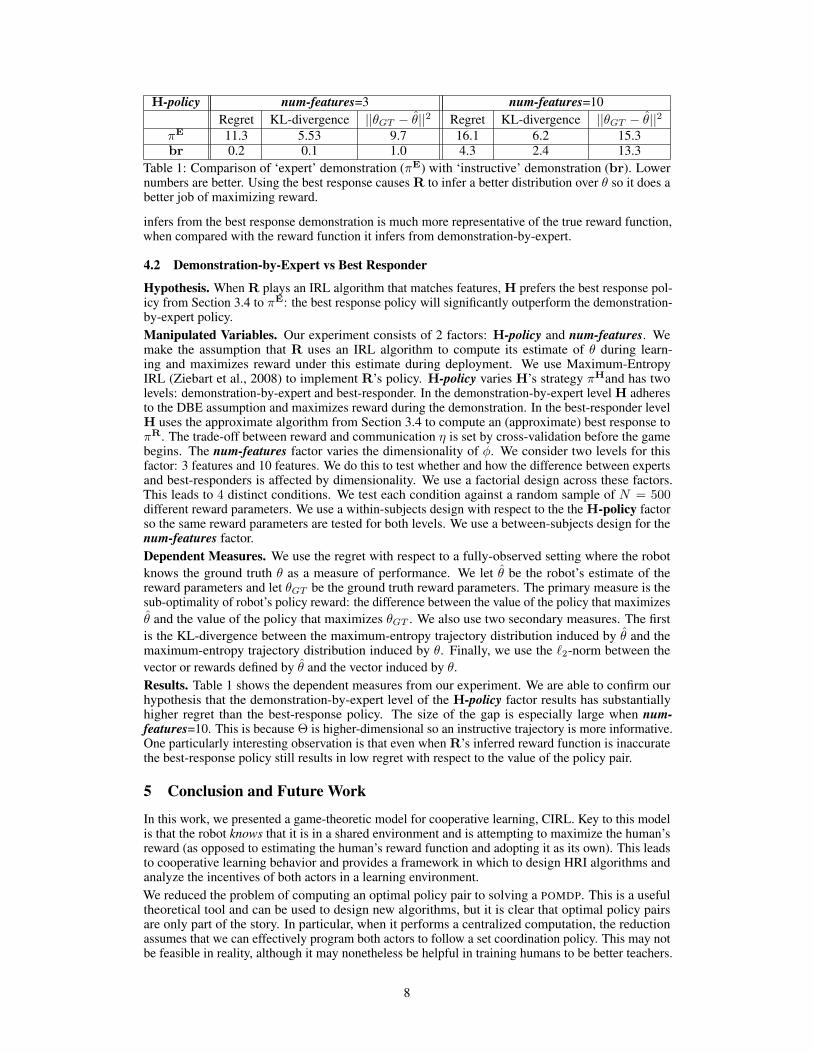
H-policy num-features=3 num-features=10Regret KL-divergence ||θGT − θ̂||2 Regret KL-divergence ||θGT − θ̂||2

πE 11.3 5.53 9.7 16.1 6.2 15.3br 0.2 0.1 1.0 4.3 2.4 13.3

Table 1: Comparison of ‘expert’ demonstration (πE) with ‘instructive’ demonstration (br). Lowernumbers are better. Using the best response causes R to infer a better distribution over θ so it does abetter job of maximizing reward.

infers from the best response demonstration is much more representative of the true reward function,when compared with the reward function it infers from demonstration-by-expert.

4.2 Demonstration-by-Expert vs Best Responder

Hypothesis. When R plays an IRL algorithm that matches features, H prefers the best response pol-icy from Section 3.4 to πE: the best response policy will significantly outperform the demonstration-by-expert policy.Manipulated Variables. Our experiment consists of 2 factors: H-policy and num-features. Wemake the assumption that R uses an IRL algorithm to compute its estimate of θ during learn-ing and maximizes reward under this estimate during deployment. We use Maximum-EntropyIRL (Ziebart et al., 2008) to implement R’s policy. H-policy varies H’s strategy πHand has twolevels: demonstration-by-expert and best-responder. In the demonstration-by-expert level H adheresto the DBE assumption and maximizes reward during the demonstration. In the best-responder levelH uses the approximate algorithm from Section 3.4 to compute an (approximate) best response toπR. The trade-off between reward and communication η is set by cross-validation before the gamebegins. The num-features factor varies the dimensionality of φ. We consider two levels for thisfactor: 3 features and 10 features. We do this to test whether and how the difference between expertsand best-responders is affected by dimensionality. We use a factorial design across these factors.This leads to 4 distinct conditions. We test each condition against a random sample of N = 500different reward parameters. We use a within-subjects design with respect to the the H-policy factorso the same reward parameters are tested for both levels. We use a between-subjects design for thenum-features factor.Dependent Measures. We use the regret with respect to a fully-observed setting where the robotknows the ground truth θ as a measure of performance. We let θ̂ be the robot’s estimate of thereward parameters and let θGT be the ground truth reward parameters. The primary measure is thesub-optimality of robot’s policy reward: the difference between the value of the policy that maximizesθ̂ and the value of the policy that maximizes θGT . We also use two secondary measures. The firstis the KL-divergence between the maximum-entropy trajectory distribution induced by θ̂ and themaximum-entropy trajectory distribution induced by θ. Finally, we use the `2-norm between thevector or rewards defined by θ̂ and the vector induced by θ.Results. Table 1 shows the dependent measures from our experiment. We are able to confirm ourhypothesis that the demonstration-by-expert level of the H-policy factor results has substantiallyhigher regret than the best-response policy. The size of the gap is especially large when num-features=10. This is because Θ is higher-dimensional so an instructive trajectory is more informative.One particularly interesting observation is that even when R’s inferred reward function is inaccuratethe best-response policy still results in low regret with respect to the value of the policy pair.

5 Conclusion and Future Work

In this work, we presented a game-theoretic model for cooperative learning, CIRL. Key to this modelis that the robot knows that it is in a shared environment and is attempting to maximize the human’sreward (as opposed to estimating the human’s reward function and adopting it as its own). This leadsto cooperative learning behavior and provides a framework in which to design HRI algorithms andanalyze the incentives of both actors in a learning environment.We reduced the problem of computing an optimal policy pair to solving a POMDP. This is a usefultheoretical tool and can be used to design new algorithms, but it is clear that optimal policy pairsare only part of the story. In particular, when it performs a centralized computation, the reductionassumes that we can effectively program both actors to follow a set coordination policy. This may notbe feasible in reality, although it may nonetheless be helpful in training humans to be better teachers.

8

An important avenue for future research will be to consider the problem of equilibrium acquisition:the process by which two independent actors arrive at an equilibrium pair of policies. Returning toWiener’s warning, we believe that the best solution is not to put a specific purpose into the machineat all, but instead to design machines that provably converge to the right purpose as they go along.

Acknowledgements

This work was supported by the DARPA Simplifying Complexity in Scientific Discovery (SIMPLEX)program. Dylan Hadfield-Menell is supported by a NSF Graduate Reseach Fellowship.

9

ReferencesAbbeel, P and Ng, A. Apprenticeship learning via inverse reinforcement learning. In ICML, 2004.

Balbach, F and Zeugmann, T. Recent developments in algorithmic teaching. In Language and Automata Theoryand Applications. Springer, 2009.

Bernstein, D, Zilberstein, S, and Immerman, N. The complexity of decentralized control of Markov decisionprocesses. In UAI, 2000.

Bostrom, N. Superintelligence: Paths, dangers, strategies. Oxford, 2014.

Boutilier, Craig. Sequential optimality and coordination in multiagent systems. In IJCAI, volume 99, pp.478–485, 1999.

Cakmak, M and Lopes, M. Algorithmic and human teaching of sequential decision tasks. In AAAI, 2012.

Dragan, A and Srinivasa, S. Generating legible motion. In Robotics: Science and Systems, 2013.

Fern, A, Natarajan, S, Judah, K, and Tadepalli, P. A decision-theoretic model of assistance. JAIR, 50(1):71–104,2014.

Gibbons, R. Incentives in organizations. Technical report, National Bureau of Economic Research, 1998.

Goldman, S and Kearns, M. On the complexity of teaching. Journal of Computer and System Sciences, 50(1):20–31, 1995.

Goldman, S, Rivest, R, and Schapire, R. Learning binary relations and total orders. SIAM Journal on Computing,22(5):1006–1034, 1993.

Golland, D, Liang, P, and Klein, D. A game-theoretic approach to generating spatial descriptions. In EMNLP,pp. 410–419, 2010.

Holmstrom, B and Milgrom, P. Aggregation and linearity in the provision of intertemporal incentives. Econo-metrica, pp. 303–328, 1987.

Holmstrom, B and Milgrom, P. Multitask principal-agent analyses: Incentive contracts, asset ownership, and jobdesign. Journal of Law, Economics, & Organization, 7:24–52, 1991.

Jensen, M and Meckling, W. Theory of the firm: Managerial behavior, agency costs and ownership structure.Journal of Financial Economics, 3(4):305–360, 1976.

Kerr, S. On the folly of rewarding A, while hoping for B. Academy of Management Journal, 18(4):769–783,1975.

Kuleshov, V and Schrijvers, O. Inverse game theory. Web and Internet Economics, 2015.

Leveson, N and Turner, C. An investigation of the Therac-25 accidents. IEEE Computer, 26(7):18–41, 1993.

Natarajan, S, Kunapuli, G, Judah, K, Tadepalli, P, and Kersting, Kand Shavlik, J. Multi-agent inverse reinforce-ment learning. In Int’l Conference on Machine Learning and Applications, 2010.

Nayyar, A, Mahajan, A, and Teneketzis, D. Decentralized stochastic control with partial history sharing: Acommon information approach. IEEE Transactions on Automatic Control, 58(7):1644–1658, 2013.

Ng, A and Russell, S. Algorithms for inverse reinforcement learning. In ICML, 2000.

Ramachandran, D and Amir, E. Bayesian inverse reinforcement learning. In IJCAI, 2007.

Ratliff, N, Bagnell, J, and Zinkevich, M. Maximum margin planning. In ICML, 2006.

Russell, S. and Norvig, P. Artificial Intelligence. Pearson, 2010.

Russell, Stuart J. Learning agents for uncertain environments (extended abstract). In COLT, 1998.

Waugh, K, Ziebart, B, and Bagnell, J. Computational rationalization: The inverse equilibrium problem. In ICML,2011.

Wiener, N. Some moral and technical consequences of automation. Science, 131, 1960.

Ziebart, B, Maas, A, Bagnell, J, and Dey, A. Maximum entropy inverse reinforcement learning. In AAAI, 2008.

10