Cooperative Base Stations for Green Cellular Networks

Choungmo Fofack Nicaise Eric

nicaiseeric@gmail.com

Master UBINET

February 24, 2010

Abstract

In this paper we make a survey of some models that have been proposed to tackle the problem

of cellular networks power consumption. We show the relevant aspects of each model, in order to

characterize the parameters that we should take in account to achieve an efficient energy saving.

1 Introduction

According to [1] “wireless communications are expected to be a major worldwide cause of energy con-sumption within few years, with a high impact on carbon dioxide emissions.”. This is not really surprisingwhen we take a general view of cellular networks. For instance, cellular networks are quite ubiquitoustoday, we can use our mobile almost every time and everywhere, that means the infrastructure deployedto provide this service is always turned on, in fact most of the time. We can easily understand why [1]shows that the real cost of networks is not anymore the capital expenditures (CAPEX, cost to deployor install the network) but the operational expenditures (OPEX, cost to maintain the availability of theservices) due to the base stations maintenance. In section 2, we report on the models proposed by dif-ferent researchers to build a green network by cooperation at the base stations level. In section 3, we goone step further to show that the cooperation at network level can improve energy savings. Then section4 presents some techniques to enforce an energy efficient network. At the end, section 5 summarizes andconcludes the survey.

2 Energy savings by cooperation at the base stations level

In this section, the models presented show how to reduce the power consumption with respect to twomain constraints: (i) the minimum coverage and (ii) the minimum required quality of service. Withrespect to the previous constraints, each model provides different outcomes by applying the cooperationbetween the the base stations of an operator’s network.

2.1 Power saving-oriented network and capacity planning model

The model in [1] is an easy and a simple analytical model that provides the degree of redundancy of anetwork to achieve a given energy saving. The authors, V. Mancuso and S. Alouf, propose to minimizethe allowable and activable number of base stations with respect to (i) and (ii); that leads to the increaseof the potential energy saving.

Assumptions: the operational consumption of a base station does not appreciably change with the traffic,

1

for a given capacity. The operational cost basically consists of two parts: a fixed part, CF , which isincurred just by turning on the site and a second part, CC , related to the capacity used at the basestation. This cost is described by the following equation:

Cpstot(t) = CF RB(t) + CC

RB(t)∑

i=1

γ(i)(t), (1)

where γ(i)(t) denotes the capacity of the i-th active base station at time t, and RB(t) ≤ NB is thenumber of active base stations, at time t, out of the total number of NB base stations deployed withinthe network. Cps

tot changes over time and is upper bounded by the cost with no power saving.

Methodology: the constraint (i) defines the minimum number of base stations to cover all the area,and according to (ii), the active base stations should hold the QoS requirements and guarantee a fullcoverage. So the number RB(t) has a lower bound which depends on the traffic offered at a given timet, and the minimum number of base station in the covered area A. This lower bound is given by thefollowing equation:

RB(t) ≥ RminB (t) = max

{⌈

A

AC

⌉

,min {⌈ρ(t)⌉ , ⌈ρmax⌉}

}

. (2)

According to (2) the choice of RB represents a limitation on the power that can be saved by turning offsome base stations completely, and the choice of NB represents the degree of the network coverage.

Results: this model has a huge impact on cell planning, it gives the minimum level of coverage re-dundancy, i.e, NB = Nmin

B if we want to achieve a targeted power savings S. Then following equationevaluates this power saving which is the difference between the total cost of network with all deployedbase stations working at full capacity, and the cost of the optimized network running with RB(t) activebase stations:

S = CF

(

NminB − RB

)

+ CC

(

NminB − ρ

)

, (3)

where RB and ρ are the averages over time and probability of RB(t) and ρ(t), respectively. It is obviousto see that S increases with NB , so this model concludes that: the availability of a dense and redundantnetwork coverage is a necessary condition for energy efficiency consumption in a cellular network.

2.2 Traffic pattern and network topology model

The model in [2] proposes another view of the problem. As the network’s operators already exist, wecan compute the potential energy saving but we do not know when to turn off a base station and how toenforce the cooperation of base stations in the network. Hence the authors propose to switch off a basestation during a period of time according to its traffic’s variation and the topology of the network [2].For this model, the main idea is to reduce the number of active cells in the access network during theperiod the normalized traffic f(t) (0 ≤ f(t) ≤ 1) in the network is low. This model is based on trafficestimation and people behaviors. For example one may turn off some base stations in residential areasduring the day because people are moving in general to the town centers, and in offices areas during thenight.

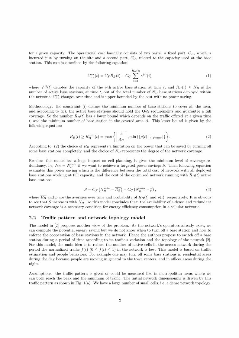
Assumptions: the traffic pattern is given or could be measured like in metropolitan areas where wecan both reach the peak and the minimum of traffic. The initial network dimensioning is driven by thistraffic pattern as shown in Fig. 1(a). We have a large number of small cells, i.e, a dense network topology.

2

(a) Traffic pattern (b) Network topology

Figure 1: In sub-figure (a), we give a simple symmetric curve around T/2, that describes the load of thenetwork during a period T . Sub-figure (b) represents a hexagonal three-sectorial network and shows howdense the initial network should be if we target a good power saving.

Note that it has been concluded by the previous model that the redundancy is a required feature of thenetwork.

Methodology: During the “night zone”, the minimum coverage and QoS are handled by a fractionx of active base stations, and the remaining 1 − x fraction is switched off. Let us call Sc this scenario.Therefore, the new traffic f (Sc)(t) received by the active base stations is equal to their own traffic, plusthe handover traffic. The total consumption C(τ) can be easily written as a sum of the consumptionduring the “day” (the time intervals [O, τ ] and [T − τ, T ], when x = 1) and the consumption in the “nightzone” (the time interval [τ, T − τ ], when x = f(τ) = f(T − τ)). Hence, we have the following equations:

f (Sc)(t) = f(t) +1 − x

xf(t) =

1

xf(t), (4)

C(τ) = 2

[

Wτ + Wf(τ)

(

T

2− τ

)]

, (5)

where W denotes the power consumption per cell. So the power saving per cell, NetSaving, is a functionof the time, the total consumption of a cell, and the value of the current traffic, as shown in the followingformula:

NetSaving = 1 −C(τ)

WT. (6)

Then, the aim is to find the optimal value τm of τ that maximizes the NetSaving, this corresponds tominimizing the total consumption of a cell C(τ). By derivation of C(τ), we attain an equation that τm

verifies:

f(τm) − f ′(τm)

(

T

2− τm

)

− 1 = 0. (7)

At the end, the base stations are not turned off randomly but with respect to the initial topology. InFig. 1(b) for example, three bases stations out of four are switched off and the remaining base station

3

increases its transmitting power.

Results: The power consuming function does not depend on topology, hence regardless of a specificconfiguration of the network, there is room for considerable energy saving by adopting some simplepower-off scheme. Moreover the simulations performed with a real measured traffic pattern of an Italianbroadband service provider, show that one can save from 25% to 30% of the total consumption [2].

2.3 Area power consumption model

Since density is a network property that enhances the coverage and the QoS, we need a mean to comparethe power consumption of different networks having different size. The paper [3] proposes a new metricbased on power consumption of the base stations and regardless of the size of the network. One canchange the topology and the density of a network in order to achieve a good coverage, an area spec-tral efficiency and, of course, the best energy saving with respect to the same value of this new metric.The paper investigates the impact of deployment strategies on the power consumption of mobile radionetwork. Improved deployment strategies lower the number of sites required in the network to fulfillperformance metrics such as coverage and area spectral efficiency. Since increasing inter-site distance Dgenerates larger coverage areas, this paper introduces the concept of area power consumption as a metricrather than using the common power consumption per site metric to compare networks differing by theirsite density, and therefore to assess the power consumption of the network relative to its size. The aimis to quantify the energy savings through deployment of micro sites alongside conventional macro sites.

Assumptions: the traffic density is uniformly distributed over the Euclidean plane. With respect toenergy needs, the paper states that network topologies featuring high density deployments of small, lowpower base stations yield strong improvements compared to low density deployments of few high powerbase stations.

Methodology: The network’s layouts consist of a varying numbers of micro base station per cell inaddition to the conventional macro sites. For both base station types, their power consumption dependson the size of the covered area as well as the degree of coverage required. For example, in urban areas cellradii usually range from about 500 m to 2500 m with coverage of more than 90%. The authors use a sim-ple linear model to link the power consumption of a site s to the average radiated power: Ps = asPtx +bs,where Ps denotes the average consumed power per site (Ps = Pma if it is a macro site and Ps = Pmi ifit is a micro site) and Ptx the radiated power per site. The coefficient as (ama or ami) accounts for thepower consumption that scales with the average radiated power due to amplifier and feeder losses as wellas cooling of sites. The term bs (bma or bmi) denotes power offsets which are consumed independentlyof the average transmit power. The power consumption of macro sites is virtually independent of trafficload. In contrast, the ability to scale their power consumption with the current activity level is consideredone major benefit of micro sites. Consequently, the parameters as and bs should depend on the trafficload. We use three metrics:- the cell coverage (defined as the fraction of cell area where the received power is above a certain levelPmin)

C =1

AC

∫

AC

r Prob (Prx(r) ≥ Pmin) dr dφ, (8)

where Prx is the received power at a distance r from the site. Given the minimum received power Pmin,

we compute the power Ptx that should be transmitted: Ptx = Pmin

K

(

C3

)λ

2 Dλ. We recall that D is theinter site distance, λ is the path loss exponent.

- the area spectral efficiency, defined as the mean of the overall spectral efficiency in the reference cell

4

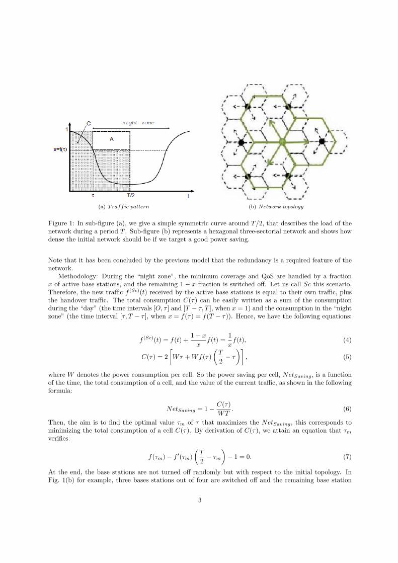
Figure 2: Area power consumption as function of inter site distance for different deployments withC = 95%, ama = 22.6 and bma = 412.4 W , ami = 5.5 and bmi = 32.0 W .

divided by the cell size and commonly measured in bit per second per Hertz per square kilometer.

- the area power consumption defined as the average power consumed in a cell divided by the corre-sponding average cell area:

P =PC

AC

. (9)

In eq. (9), AC =√

32 D2 and the power consumption per cell PC is computed by adding the power

of the macro site Pma to the average power NPmi of N micro sites located in the same cell, i.e.,PC = Pma + NPmi. The area power consumption is measured in Watts per square kilometer. Thenthe area power consumption P is a density of power per area (power consumption per cell over the cellarea).

Results: For λ = 2 , P is not affected by the site distance D since the PC and AC increase with D2.For λ > 2 , there exists a positive site distance D∗ which minimizes the area power consumption of thenetwork as the Fig. 2 shows.The deployment of micro sites allows to significantly decrease the area power consumption in the networkwhile still achieving certain area throughput targets, and this deployment strongly depends on the offsetpower consumption of both macro and micro sites.

3 Energy savings by cooperation at the network level

In this section, we will introduce the notion of “sleep mode”. We will not introduce it at the basestation level, but at the system level (a cooperation between an operator’s systems, a 2G/3G networkfor example), and further at the network level(a cooperation among operators). Many researchers haveinvestigated the impact of these approaches on the total energy savings [4] [5].

3.1 System selection within an operator’s network

The model in [4] tackles the power saving problem from the radio resource management perspective.The authors develop a system selection algorithm for heterogeneous networks like 2G/3G networks. In

5

(a) Blocking rate (b) Energy consumption

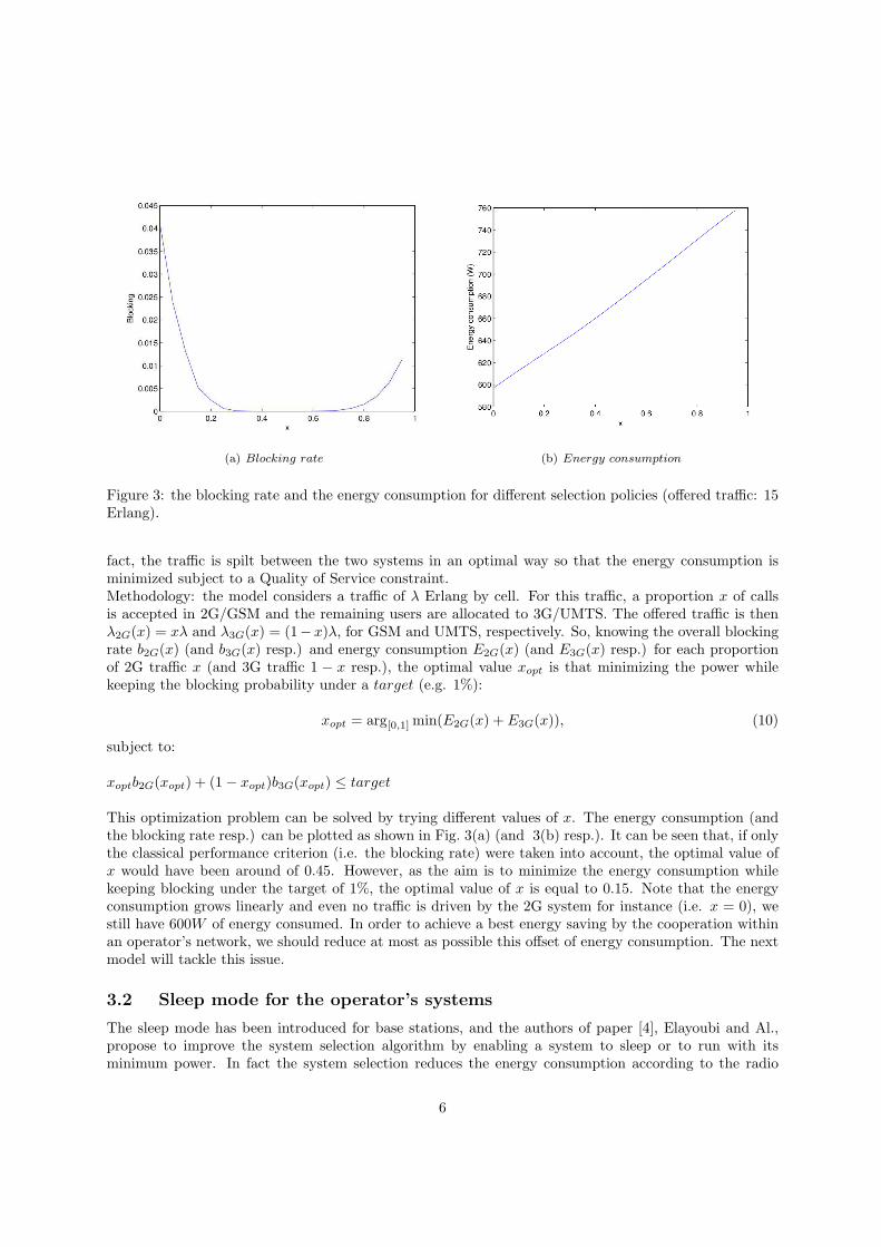
Figure 3: the blocking rate and the energy consumption for different selection policies (offered traffic: 15Erlang).

fact, the traffic is spilt between the two systems in an optimal way so that the energy consumption isminimized subject to a Quality of Service constraint.Methodology: the model considers a traffic of λ Erlang by cell. For this traffic, a proportion x of callsis accepted in 2G/GSM and the remaining users are allocated to 3G/UMTS. The offered traffic is thenλ2G(x) = xλ and λ3G(x) = (1−x)λ, for GSM and UMTS, respectively. So, knowing the overall blockingrate b2G(x) (and b3G(x) resp.) and energy consumption E2G(x) (and E3G(x) resp.) for each proportionof 2G traffic x (and 3G traffic 1 − x resp.), the optimal value xopt is that minimizing the power whilekeeping the blocking probability under a target (e.g. 1%):

xopt = arg[0,1] min(E2G(x) + E3G(x)), (10)

subject to:

xoptb2G(xopt) + (1 − xopt)b3G(xopt) ≤ target

This optimization problem can be solved by trying different values of x. The energy consumption (andthe blocking rate resp.) can be plotted as shown in Fig. 3(a) (and 3(b) resp.). It can be seen that, if onlythe classical performance criterion (i.e. the blocking rate) were taken into account, the optimal value ofx would have been around of 0.45. However, as the aim is to minimize the energy consumption whilekeeping blocking under the target of 1%, the optimal value of x is equal to 0.15. Note that the energyconsumption grows linearly and even no traffic is driven by the 2G system for instance (i.e. x = 0), westill have 600W of energy consumed. In order to achieve a best energy saving by the cooperation withinan operator’s network, we should reduce at most as possible this offset of energy consumption. The nextmodel will tackle this issue.

3.2 Sleep mode for the operator’s systems

The sleep mode has been introduced for base stations, and the authors of paper [4], Elayoubi and Al.,propose to improve the system selection algorithm by enabling a system to sleep or to run with itsminimum power. In fact the system selection reduces the energy consumption according to the radio

6

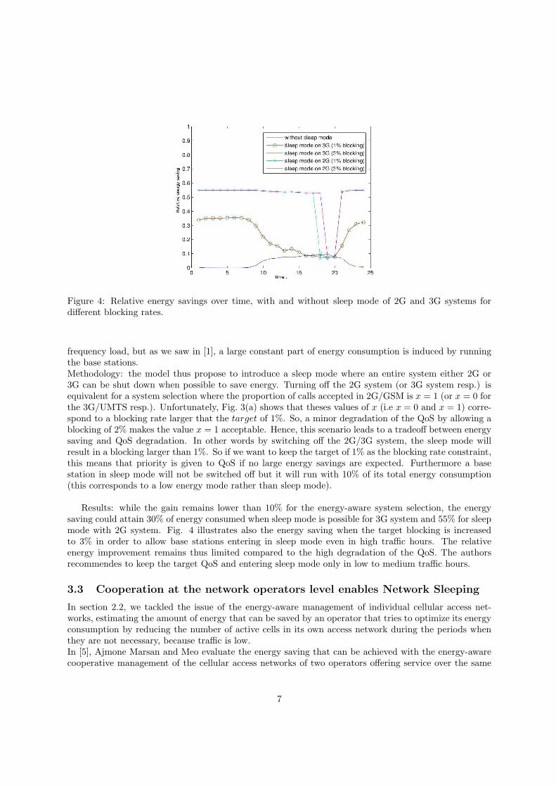
Figure 4: Relative energy savings over time, with and without sleep mode of 2G and 3G systems fordifferent blocking rates.

frequency load, but as we saw in [1], a large constant part of energy consumption is induced by runningthe base stations.Methodology: the model thus propose to introduce a sleep mode where an entire system either 2G or3G can be shut down when possible to save energy. Turning off the 2G system (or 3G system resp.) isequivalent for a system selection where the proportion of calls accepted in 2G/GSM is x = 1 (or x = 0 forthe 3G/UMTS resp.). Unfortunately, Fig. 3(a) shows that theses values of x (i.e x = 0 and x = 1) corre-spond to a blocking rate larger that the target of 1%. So, a minor degradation of the QoS by allowing ablocking of 2% makes the value x = 1 acceptable. Hence, this scenario leads to a tradeoff between energysaving and QoS degradation. In other words by switching off the 2G/3G system, the sleep mode willresult in a blocking larger than 1%. So if we want to keep the target of 1% as the blocking rate constraint,this means that priority is given to QoS if no large energy savings are expected. Furthermore a basestation in sleep mode will not be switched off but it will run with 10% of its total energy consumption(this corresponds to a low energy mode rather than sleep mode).

Results: while the gain remains lower than 10% for the energy-aware system selection, the energysaving could attain 30% of energy consumed when sleep mode is possible for 3G system and 55% for sleepmode with 2G system. Fig. 4 illustrates also the energy saving when the target blocking is increasedto 3% in order to allow base stations entering in sleep mode even in high traffic hours. The relativeenergy improvement remains thus limited compared to the high degradation of the QoS. The authorsrecommendes to keep the target QoS and entering sleep mode only in low to medium traffic hours.

3.3 Cooperation at the network operators level enables Network Sleeping

In section 2.2, we tackled the issue of the energy-aware management of individual cellular access net-works, estimating the amount of energy that can be saved by an operator that tries to optimize its energyconsumption by reducing the number of active cells in its own access network during the periods whenthey are not necessary, because traffic is low.In [5], Ajmone Marsan and Meo evaluate the energy saving that can be achieved with the energy-awarecooperative management of the cellular access networks of two operators offering service over the same

7

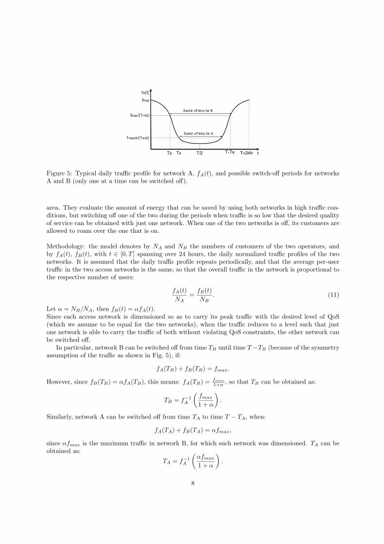
Figure 5: Typical daily traffic profile for network A, fA(t), and possible switch-off periods for networksA and B (only one at a time can be switched off).

area. They evaluate the amount of energy that can be saved by using both networks in high traffic con-ditions, but switching off one of the two during the periods when traffic is so low that the desired qualityof service can be obtained with just one network. When one of the two networks is off, its customers areallowed to roam over the one that is on.

Methodology: the model denotes by NA and NB the numbers of customers of the two operators, andby fA(t), fB(t), with t ∈ [0, T ] spanning over 24 hours, the daily normalized traffic profiles of the twonetworks. It is assumed that the daily traffic profile repeats periodically, and that the average per-usertraffic in the two access networks is the same, so that the overall traffic in the network is proportional tothe respective number of users:

fA(t)

NA

=fB(t)

NB

. (11)

Let α = NB/NA, then fB(t) = αfA(t).Since each access network is dimensioned so as to carry its peak traffic with the desired level of QoS(which we assume to be equal for the two networks), when the traffic reduces to a level such that justone network is able to carry the traffic of both without violating QoS constraints, the other network canbe switched off.

In particular, network B can be switched off from time TB until time T −TB (because of the symmetryassumption of the traffic as shown in Fig. 5), if:

fA(TB) + fB(TB) = fmax.

However, since fB(TB) = αfA(TB), this means: fA(TB) = fmax

1+α, so that TB can be obtained as:

TB = f−1A

(

fmax

1 + α

)

.

Similarly, network A can be switched off from time TA to time T − TA, when:

fA(TA) + fB(TA) = αfmax,

since αfmax is the maximum traffic in network B, for which such network was dimensioned. TA can beobtained as:

TA = f−1A

(

αfmax

1 + α

)

.

8

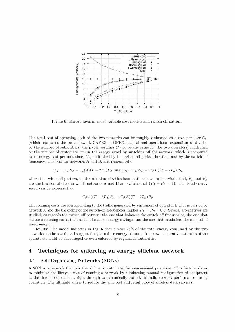
Figure 6: Energy savings under variable cost models and switch-off pattern.

The total cost of operating each of the two networks can be roughly estimated as a cost per user CU

(which represents the total network CAPEX + OPEX capital and operational expenditures dividedby the number of subscribers; the paper assumes CU to be the same for the two operators) multipliedby the number of customers, minus the energy saved by switching off the network, which is computedas an energy cost per unit time, Ce, multiplied by the switch-off period duration, and by the switch-offfrequency. The cost for networks A and B, are, respectively:

CA = CUNA − Ce(A)(T − 2TA)PA and CB = CUNB − Ce(B)(T − 2TB)PB ,

where the switch-off pattern, i.e the selection of which base stations have to be switched off, PA and PB

are the fraction of days in which networks A and B are switched off (PA + PB = 1). The total energysaved can be expressed as:

Ce(A)(T − 2TA)PA + Ce(B)(T − 2TB)PB .

The roaming costs are corresponding to the traffic generated by customers of operator B that is carried bynetwork A and the balancing of the switch-off frequencies implies PA = PB = 0.5. Several alternatives arestudied, as regards the switch-off pattern: the one that balances the switch-off frequencies, the one thatbalances roaming costs, the one that balances energy savings, and the one that maximizes the amount ofsaved energy.

Results: The model indicates in Fig. 6 that almost 25% of the total energy consumed by the twonetworks can be saved, and suggest that, to reduce energy consumption, new cooperative attitudes of theoperators should be encouraged or even enforced by regulation authorities.

4 Techniques for enforcing an energy efficient network

4.1 Self Organizing Networks (SONs)

A SON is a network that has the ability to automate the management processes. This feature allowsto minimize the lifecycle cost of running a network by eliminating manual configuration of equipmentat the time of deployment, right through to dynamically optimizing radio network performance duringoperation. The ultimate aim is to reduce the unit cost and retail price of wireless data services.

9

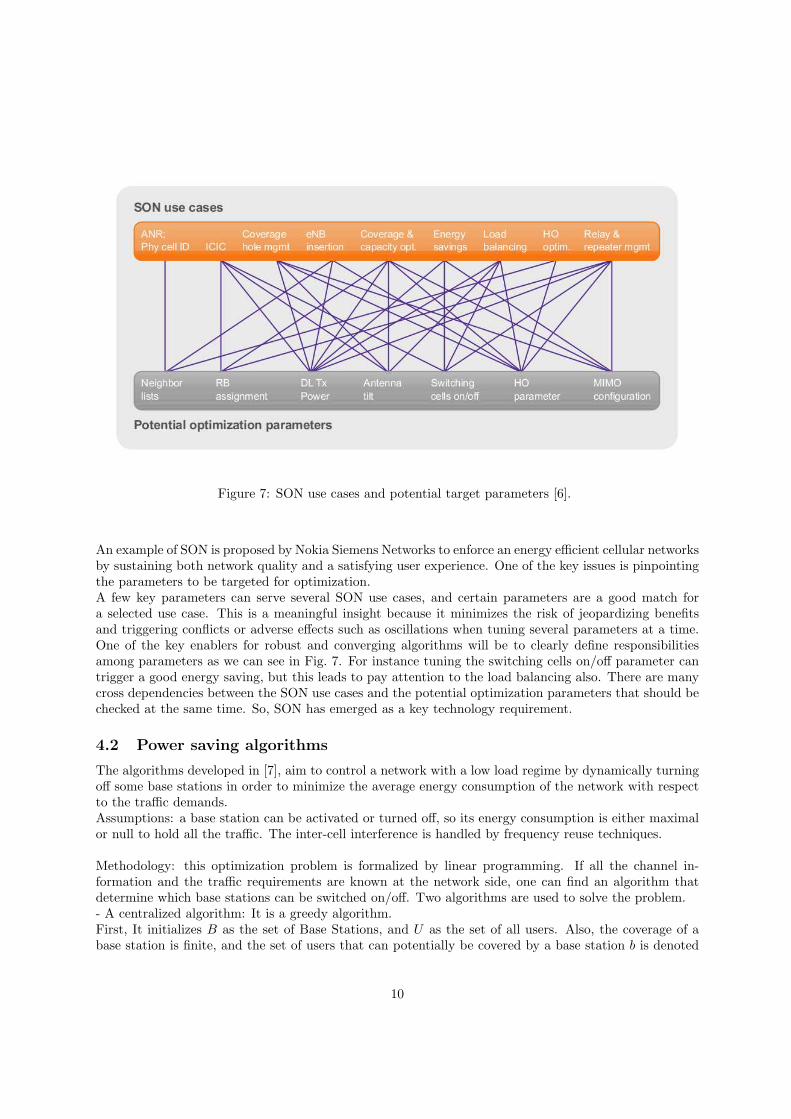
Figure 7: SON use cases and potential target parameters [6].

An example of SON is proposed by Nokia Siemens Networks to enforce an energy efficient cellular networksby sustaining both network quality and a satisfying user experience. One of the key issues is pinpointingthe parameters to be targeted for optimization.A few key parameters can serve several SON use cases, and certain parameters are a good match fora selected use case. This is a meaningful insight because it minimizes the risk of jeopardizing benefitsand triggering conflicts or adverse effects such as oscillations when tuning several parameters at a time.One of the key enablers for robust and converging algorithms will be to clearly define responsibilitiesamong parameters as we can see in Fig. 7. For instance tuning the switching cells on/off parameter cantrigger a good energy saving, but this leads to pay attention to the load balancing also. There are manycross dependencies between the SON use cases and the potential optimization parameters that should bechecked at the same time. So, SON has emerged as a key technology requirement.

4.2 Power saving algorithms

The algorithms developed in [7], aim to control a network with a low load regime by dynamically turningoff some base stations in order to minimize the average energy consumption of the network with respectto the traffic demands.Assumptions: a base station can be activated or turned off, so its energy consumption is either maximalor null to hold all the traffic. The inter-cell interference is handled by frequency reuse techniques.

Methodology: this optimization problem is formalized by linear programming. If all the channel in-formation and the traffic requirements are known at the network side, one can find an algorithm thatdetermine which base stations can be switched on/off. Two algorithms are used to solve the problem.- A centralized algorithm: It is a greedy algorithm.First, It initializes B as the set of Base Stations, and U as the set of all users. Also, the coverage of abase station is finite, and the set of users that can potentially be covered by a base station b is denoted

10

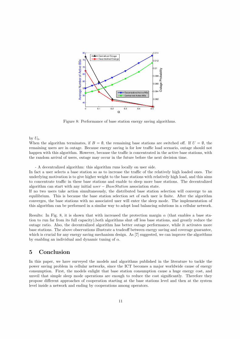
Figure 8: Performance of base station energy saving algorithms.

by Ub.When the algorithm terminates, if B = ∅, the remaining base stations are switched off. If U = ∅, theremaining users are in outage. Because energy saving is for low traffic load scenario, outage should nothappen with this algorithm. However, because the traffic is concentrated in the active base stations, withthe random arrival of users, outage may occur in the future before the next decision time.

- A decentralized algorithm: this algorithm runs locally on user side.In fact a user selects a base station so as to increase the traffic of the relatively high loaded ones. Theunderlying motivation is to give higher weight to the base stations with relatively high load, and this aimsto concentrate traffic in these base stations and enable to sleep more base stations. The decentralizedalgorithm can start with any initial user − BaseStation association state.If no two users take action simultaneously, the distributed base station selection will converge to anequilibrium. This is because the base station selection set of each user is finite. After the algorithmconverges, the base stations with no associated user will enter the sleep mode. The implementation ofthis algorithm can be performed in a similar way to adopt load balancing solutions in a cellular network.

Results: In Fig. 8, it is shown that with increased the protection margin α (that enables a base sta-tion to run far from its full capacity),both algorithms shut off less base stations, and greatly reduce theoutage ratio. Also, the decentralized algorithm has better outage performance, while it activates morebase stations. The above observations illustrate a tradeoff between energy saving and coverage guarantee,which is crucial for any energy saving mechanism design. As [7] suggested, we can improve the algorithmsby enabling an individual and dynamic tuning of α.

5 Conclusion

In this paper, we have surveyed the models and algorithms published in the literature to tackle thepower saving problem in cellular networks, since the ICT becomes a major worldwide cause of energyconsumption. First, the models enlight that base station consumption cause a huge energy cost, andunveil that simple sleep mode operations are enough to reduce the cost significantly. Therefore theypropose different approaches of cooperation starting at the base stations level and then at the systemlevel inside a network and ending by cooperations among operators.

11

For the cooperation at the base stations level, model’s outcomes are very interesting since one can computethe power saving, the minimum number of base stations (section 2.1), one can switch off the base stationaccording to the existing network topology (section 2.2) and compare the different networks obtainedwith different switch off schemes (section 2.3).At the network level, the paper reports how an operator can efficiently use its network by applying acooperation between its different deployed systems to achieve a large energy saving. The paper showsthat a cooperation between operators is really possible and can reduce the total consumption of ICT atregional, national or international level.In the final part, the paper emphazises some techniques and algorithms proposed to enforce an energyefficient network.

References

[1] V. Mancuso and S. Alouf, “Making the base station green: a survey on strategies for reducing costand pollution in wideband cellular networks,” 2009.

[2] M. Ajmone Marsan, L. Chiaraviglio, D. Ciullo, and M. Meo, “Optimal energy savings in cellularaccess networks,” in Proc. IEEE ICC09 Workshop, GreenComm’09, June 2009.

[3] A. Fehske, F. Richter, and G. Fettweis, “Energy Efficiency Improvements through Micro Sites in Cellu-lar Mobile Radio Networks,” in Proceedings of the International Workshop on Green Communications(GreenComm’09), Honolulu, USA, 30 Nov - 04 Dec 2009.

[4] L. Saker, S. E. Elayoubi, and H. O. Scheck, “Energy-aware system selection in cooperative networks,”in Proc. of VTC Fall, 2009.

[5] M. Ajmone Marsan and M. Meo, “Energy efficient management of two cellular access networks,” inGreenMetrics 2009 Workshop (In conjunction with ACM SIGMETRICS / Performance 2009), 2009.

[6] Nokia Siemens Networks, “Introducing the Nokia Siemens Networks SON suite - an efficient, future-proof platform for SON,” Nov. 2009.

[7] S. Zhou, J. Gong, Z. Yang, Z. Niu, and P. Yang, “Green Mobile Access Network with Dynamic BaseStation Energy Saving,” IEICE, Tech. Rep. vol. 109, no. 262, IA2009-50, pp. 25-29, Oct. 2009.

12