Convolutive modelling of electrochemical processes based on the relationship between the current and the surface concentration

Journal of Electroanalytical Chemistry 464 (1999) 1–13

Convolutive modelling of electrochemical processes based on therelationship between the current and the surface concentration

Peter J. Mahon, Keith B. Oldham *

Chemistry Department, Trent Uni6ersity, Peterborough, Ont., K9J 7B8, Canada

Received 22 January 1998; received in revised form 5 November 1998

Abstract

Three of the fundamental variables in voltammetry are the faradaic current I(t) and the surface concentrations c sR (t) and c s

P (t)of the reactant and product. This article explores the relationships between these variables for cases in which the surfaceconcentrations are uniform. Convolutions are derived which permit interconversion between the current and the surfaceconcentrations. Examples are presented that apply to various electrode geometries, with and without the participation ofhomogeneous kinetics. An intriguingly simple connection is established between the convolution required for the I(t)�c s (t)conversion and that applicable to the converse c s (t)�I(t) transformation. These operations may be exploited in modellingvoltammetric experiments and several exemplars are developed. © 1999 Elsevier Science S.A. All rights reserved.

Keywords: Voltammetric modelling; Convolution integral; Semiintegration; Cyclic voltammetry; Chronoamperometry; Chrono-coulometry

1. Introduction

For more than a quarter century it has been recog-nized that, for the electron-transfer reaction

Rsoln−ne− = Psoln (1)

there is a general relationship linking the concentra-tions, c s

R (t) and c sP (t), of the reactant R and product P

at the electrode surface to the faradaic current I(t).This classical relationship is ‘general’ in the sense that itapplies to any voltammetric technique and is indepen-dent of the reversibility or mechanism of reaction (1).However the validity of the relationship requires thatno homogeneous reactions are experienced by R or Pand that transport to and from the electrode is byplanar semiinfinite diffusion.

The relationships in question may be written as

DR DcR(t)=DP DcP(t)=M(t)nFA

(2)

where A is the electrode area, F is Faraday’s constant,and the Dc terms represent the absolute values of theconcentration excursions at the electrode surface,namely

Dci(t)= �c is(t)−c i

b� for i=R or P (3)

with cbR and cb

P being the bulk concentrations, the latterusually equalling zero. Di is the diffusivity (diffusioncoefficient) of species i. Note that, to match IUPAC’ssign convention for current, n is positive for an oxida-tion, negative for a reduction.

The quantity M(t) was described as the ‘faradaicsemiintegral’ by Oldham and coworkers [1–5]

M(t)=d−1/2I(t)

dt−1/2 (4a)

Saveant et al. ([6,7], using the symbolism I(t) to replaceour M(t) and i(t) to replace our I(t)), employed theterm ‘convolved current’

* Corresponding author. Tel.: +1-705-748-1336; fax: +1-705-748-1625; e-mail: [email protected].

0022-0728/99/$ - see front matter © 1999 Elsevier Science S.A. All rights reserved.PII: S 0 0 2 2 -0728 (98 )00450 -1

P.J. Mahon, K.B. Oldham / Journal of Electroanalytical Chemistry 464 (1999) 1–132

M(t)=I(t) *1

pt(4b)

where * denotes the operation of convolution, definedbelow in Eq. (7). Both descriptions are strictlyequivalent.

Because the operation in Eq. (4a) is easily accom-plished numerically, Eq. (2) provides direct access tothe concentrations of the electroactive species at theelectrode surface from the faradaic current. There isoften a need to perform the inverse calculation: topredict the faradaic current from the concentration ofeither R or P at the electrode surface. This requires thatI(t) is accessible from M(t). Again, there are equivalentdescriptions of this operation: semidifferentiation [8,9]

I(t)=d1/2M(t)

dt1/2 (5a)

or deconvolution [10]

I(t)=dM(t)

dt*

1

pt(5b)

The attractive features of the semiintegral M(t)—that it is linearly related, via constants that are usuallyknown, to the surface concentrations of both electroac-tive species—led to successful attempts to overcome thelimitations implicit in the original concept. By removingthose limitations, primarily the absence of homoge-neous reactions and restriction to planar semiinfinitegeometry, it has become possible to extend the advan-tages of the semiintegral to a wider class of voltammet-ric processes [11]. The key to the extension is to retainEq. (2), which now becomes a definition of Mi(t), in theslightly modified form

Di Dci(t)=Mi(t)nFA

for i=R or P (6)

and seek a replacement for Eq. (4b) in the form

Mi(t)=I(t)*gi(t)=& t

0

I(t)gi(t−t) dt

for i=R or P (7)

The functions gi(t) are now application specific; that is,they incorporate details of any homogeneous reactionsinvolved and/or the non-planar-semiinfinite geometry.The functions gR(t) and gP(t) are often the same, ordiffer only slightly. Notice too, that Eq. (6) defines twodifferent (though, again, often only slightly different)functions MR(t) and MP(t), whereas a single M(t) diddouble duty in Eq. (2). Though they are not semiinte-grals, the MR(t) and MP(t) functions are called ‘ex-tended semiintegrals’ [11] because they extend thebenefits of semiintegration and because they satisfy thelimits

MR(t)�d−1/2I(t)

dt−1/2 �MP(t) as t�0 (8)

that is, both extended semiintegrals degenerate to truesemiintegrals at short enough times.

Well over one dozen useful gi(t) functions have beendiscovered and placed in the literature [3,5,11–13]. Thepurpose of the present study is not to add to thiscompilation but to carry out four related tasks:� To explore the generality of the relationship

nFADi Dci(t)=I(t) * gi(t) for i=R or P(9)

which comes from combining Eqs. (6) and (7). Weshall identify circumstances in which such a relationwould be expected to hold.

� To demonstrate that, whenever there exists a gi(t)function that permits, via Eq. (9), the determinationof c s

i (t) from I(t), that there exists a conjugatefunction hi(t), such that

I(t)

nFADi

=dDci(t)

dt* hi(t) for i=R or P (10)

by which I(t) can be found from c si (t). The analogy

of Eqs. (9) and (10), to Eq. (4b) and Eq. (5b),respectively, is apparent.

� To list examples of conjugate g(t), h(t) pairs.� To demonstrate the utility of these concepts by

devising algorithms to implement them, and usingthose algorithms to model specific voltammetricproblems.

2. The generality of relationship (9)

Consider reaction (1) taking place at an electrode ofunspecified shape, in contact with a volume of solutionthrough which solutes R and P can diffuse freely, theirconcentrations being initially uniform and equal to cb

R

and cbP. Starting at the instant t=0, the electrode is

polarized and a time-dependent faradaic current flowsthereafter. Let it be postulated that this polarizationleads to a uniform, though not necessarily constant,concentration of P at all points on the electrode sur-face. This may be for one of three reasons:� The electrode is ‘uniformly accessible’, a property

restricted to a suitable plane, cylinder or sphere. Inthis case it is the symmetry of the electrode thatdictates uniformity of concentration.

� The reaction is reversible, in which case it is theuniformity of the electrical potential of the electrodewhich, via Nernst’s law, enforces the uniformity ofthe ratio of the activities of R and P at the electrodesurface. Provided that the diffusion coefficients ofthe two species are sufficiently similar, the unifor-mity of their activity ratio implies that the individualconcentrations of R and P are also uniform.

� The polarization is so intense that the concentrationof R is virtually zero on the electrode surface. In this

P.J. Mahon, K.B. Oldham / Journal of Electroanalytical Chemistry 464 (1999) 1–13 3

case, provided that the two diffusivities are similar, thesurface concentration of P will be uniform even if theelectrode reaction is not reversible. Support for theseconditions will be found in Appendix B.Let the current have a magnitude I0 during the brief

time interval 0B t5dt. This current need not necessarilybe of uniform density, even though it must give rise toa uniform concentration of P at the electrode surface.The current will continue after t=dt, but we shall cometo that later. A total amount

dN0=I0dtnF

(11)

of species P will be generated during this initial interval.Consider what the effect will be of the faradaic genera-tion of this dN0 amount of solute P at an arbitrary pointX somewhere in solution, in the vicinity of the electrode.The concentration there will sooner or later suffer anexcursion from its prevailing cb

P value by rising, thenpassing through a maximum at a time commensuratewith x2/DP, where x is the distance from X to the closestpoint on the electrode, and eventually slowly declining.If dcX

0 denotes this small concentration excursion, then

dc0X(t)=dN0 f X(t). (12)

The function f X(t) is a proportionality factor thatdepends on the location of point X and the nature of theelectrical signal. Note that the 0 subscript on dcX doesnot imply during the 0B t5dt interval, but attributableto the burst of solute generated during that interval.Combination of the last two equations leads to

dc0X(t)=

I0 f X(t)dtnF

(13)

Now turn attention to the dtB t52dt interval, duringwhich the current is I1. This will generate an amount dN1,equal to I1dt/nF, of solute P over the entire electrodesurface. If I1=I0, the effect at point X of this secondinjection of product will exactly mimic that of the firstinjection except that there is an added delay before theeffect is felt. If I1 differs from I0, there will be the samedelay but, additionally the effect will be either enhancedor diminished according as I1 is greater than or less thanI0. Either way

dc1X(t)=dN1 f X(t−dt)=

I1 f X(t−dt)dtnF

(14)

The function f X( ) in Eq. (14) is identical to that in Eq.(13) only because of our stipulation that the surfaceconcentration be uniform. Only in this circumstance1 can

we be assured that each effect at X is strictly proportionalto the total amount of solute generated during theinterval in question.

The total increase in the concentration of P at pointX is, of course, found by adding Eqs. (13) and (14). Itis then possible to generalize to a finite number ofintervals

cPX(t)=cP

b + %(t−dt)/dt

j=0

dc jX(t)

=cPb +

dtnF

%(t−dt)/dt

j=0

Ij f X(t− jdt) (15)

at time t ; or, by defining t= jdt and letting dt approachzero as j approaches infinity:

cPX(t)=cP

b +1

nF& t

0

I(t)f X(t−t) dt (16)

It is convenient to replace the f X( ) function in Eq. (16)by a gX

p ( ) function defined as f X( )A DP. Then, ontransposition and adoption of definition (3), Eq. (16)becomes

DcPX(t)=cP

X(t)−cPb =

& t

0

I(t)gPX(t−t)dt

nFA DP

(17)

The gXP ( ) function is seen to have dimensions correspond-

ing to the s−1/2 unit.Would Eq. (17) hold if the species P slowly decom-

posed, or reacted with some component of the electrolytesolution? Provided that the reaction did not destroy theproportionality between dNj and dcX

j , i.e. if the reactionwere first-order, then Eq. (17) would still apply, thoughthe function gX

P ( ) would naturally be different.The f X( ) and gX

P ( ) functions are, of course, dependentupon the location of point X. No restriction has beenplaced on this location, except that it be in the solution.A location on the electrode surface is not precluded. Infact, the most useful application of Eq. (17) is to the casewhen the point X lies on the surface. We need not thenspecify exactly where on the surface, because of theprerequisite that the surface concentration be uniform.With the absence of a superscript X taken to mean ‘onthe surface’, Eq. (17) rearranges to give

nFADP DcP(t)=& t

0

I(t)gP(t−t) dt (18)

which, in light of the definition of the convolutionoperator, is identical to the i=P version of Eq. (9). Thecase i=R can be treated by similar arguments and leadsagain to Eq. (9).

What we have just presented is an informal proof thatan equation of the form of Eq. (9) will apply in anyvoltammetric circumstance in which:� Transport is diffusive.

1 Actually this condition is stronger than is needed. It is necessaryonly that the concentrations at any two fixed points on the surfacebear a constant ratio to each other. It is unlikely, however, thatconditions would exist in which this constant ratio would have avalue other than unity.


� The concentrations of reactant and product are uni-form on the electrode surface.

� Any homogeneous reactions are first order.Although an equation of this form has been usedseveral times in the electrochemical literature, never, asfar as we aware, has it been established with this degreeof generality.

3. The conjugate function h(t)

Previously [11] we demonstrated a general numericalprocedure for voltammetric modelling which overcamethe difficulty of finding the current I(t) by deconvolvingthe gi(t) and Dci(t) functions. However, it seems plausi-ble that, if a convolution of I(t) with gi(t) producesDci(t), then some function related to gi(t) should existwhich, when convolved with Dci(t) yields I(t). We shallshow that relationships involving a putative functionhi(t) can play this role.

It is often convenient to use integral transform meth-ods when dealing with the differential equations en-countered in electrochemical problems and the Laplacetransform technique is particularly useful for situationsinvolving convolution integrals. The Laplace transformof Eq. (9) is

nFADi Dci(s)=I( (s)gi(s) for i=R or P (19)

where an overbar indicates the transform of the un-barred quantity and s is the ‘dummy’ Laplace variable.Note that the two functions I(t) and gi(t), previouslylinked via convolution in the time domain, are nowmore simply linked by multiplication in Laplace space.It therefore follows that

I( (s)

nFADi

=Dci(s)gi(s)

for i=R or P (20)

Unless the denominatorial function, gi(s) in this case, isunusually simple, it is not possible to invert a quotientof functions of s, such as the right-hand side of Eq.(20). It is for this reason that a second function isneeded.

Consider the imposition, on an electrode of anyshape but satisfying the conditions set out in Section 2,of a potential step large enough that the electroreactantconcentration at the electrode surface is diminished tozero. Then from definition (3), DcR(t)=cb

R, a constant.Accordingly, the Laplace transform, Eq. (20), of thechronoamperometric relationship adopts the form

I( (s)step

nFADR

=cR

b

sgR(s)(21)

because the Laplace transformation of a constant isequivalent to division by s. Now define

h( R(s)=1

sgR(s)(22)

then

I( (s)step

nFADR cRb=h( R(s) (23)

Laplace inversion then leads to the simple result

I(t)step

nFADR cRb=hR(t) (24)

which shows how hR(t) may be measured experimen-tally, simply by carrying out a potential-leap experi-ment. For simple electrode configurations, it is oftenpossible to calculate hi(t) functions, as will be demon-strated in a later section.

If we return to Eq. (20) and introduce definition (22),then

I( (s)

nFADi

=Dci(s)sh( i(s) for i=R or P (25)

The presence of the s multiplier in the Laplace Eq. (25)is equivalent to a differentiation operation in the timedomain performed on either Dci(t) or hi(t). However,the first option is preferred, because Laplace inversionmust generate a function bounded for t]0, whichdDci(t)/dt invariably is. Thus, we regard the right-handside of Eq. (25) as the product of functions sDci(s) andhi(s), giving, on inversion, Eq. (10) of the Introduction

I(t)

nFADi

=dDci(t)

dt* hi(t) for i=R or P (26)

This important result allows a simple convolution to beused to convert surface concentrations to currents. Eq.(26) has been derived previously [10] for the specificcase of uncomplicated planar diffusion; thence voltam-metric modelling was demonstrated using a discreteFourier transform algorithm to evaluate the convolu-tion integral.

The alternative inversion of Eq. (25), in which weregard its right-hand side as a product of Dci(s) andshi(s), leads to the convolution

I(t)

nFADi

=Dci(t) *dhi(t)

dtfor i=R or P (27)

Though mathematically less attractive than Eq. (26),this formulation presents no numerical difficulties, aswill be discovered in Section 5.

The relationship between gi(t) and hi(t) in the timedomain is not intuitively obvious but in Laplace spacea very simple relationship exists

gi(s)h( i(s)=1s

for i=R or P (28)

and therefore the inverse Laplace transform is

gi(t) * hi(t)=1 for i=R or P (29)


It is credible that the nature of the conjugate functionhi(t) will be dependent upon the electrode geometry,the geometry of the diffusion field and the presenceof homogeneous solution kinetics in a similar, yetcomplementary, manner to its corresponding gi(t)function.

The self-consistency of the convolutions can beneatly confirmed via Eqs. (9), (10) and (29). Startwith Eq. (9) and eliminate the I(t)/nFADi term viaEq. (10).

Dci(t)=dDci(t)

dt* hi(t) * gi(t) for i=R or P (30)

The distributive law applies to convolution and en-ables Eq. (29) to provide the conversion into

Dci(t)=dDci(t)

dt* 1 for i=R or P (31)

but convolution with unity is equivalent to integra-tion

dDci(t)dt

* 1=& t

0

dDci(t)dt

dt=Dci(t) for i=R or P

(32)

and the expected identity is demonstrated.

4. Examples of the conjugate function pairs

It has been noted [11] that the gi(t) functions in-variably reduce to 1/pt in the limit as t�0 and thisis also true for the hi(t) functions presented below.This is consistent with the concept of consideringMR(t) and MP(t) as extensions of the semiintegral[11]. Table 1 contains a list of interesting conjugateg(t):h(t) functions, including many used in the fol-lowing electrochemically relevant examples.

(a) A uniquely simple situation, corresponding tothe first entry in Table 1, arises for the case involvinguncomplicated planar diffusion.

gR(t)=gP(t)=hR(t)=hP(t)=1

pt(33)

(b) Under convex spherical diffusion conditionswhen the electrode has a radius of r, we have theknown result [5,13]

gi(t)=1

pt−

Di

rexp

!Ditr2

"erfc

!Ditr

"for i=R or P (34)

The erfc {} function is the error function complement[14]. This case corresponds to the second entry inTable 1 with

hi(t)=1

pt+

Di

rfor i=R or P (35)

A time-independent term in each h(t) function aug-ments the planar counterpart. This term increasinglydominates as the duration of the experiment increasesand the steady state is approached.

(c) In the situation where R is a metal ion, dis-solved in a solution, and the electrogenerated speciesP is a metal that dissolves as an amalgam and dif-fuses inside a mercury drop, gR(t) and hR(t) will bethe same as for case (b). For the product, however[13]

gP(t):1

pt

+DP

rexp

!DPtr2

"erfc

!−DPtr

"(small t) (36)

gP(t)=DP

r�

3+2 %�

p=1

exp!−yp

2DPtr2

"n(large t)

(37)

Table 1Pairs of conjugate g(t):h(t) functionsa

a All these functions approach 1/pt as t�0. Though the columnsare headed ‘g(t)’ and ‘h(t)’, these headings could equally well bereversed. b is any constant with dimensions of (time)−1/2


where yp is the p th positive root of the equation y=tan(y). The conjugate function corresponding to theninth entry in Table 1 is

hP(t)=DP

ru3!

0;DPtr2

"−

DP

r(38)

This equation is valid for all times, the u3{0; x} func-tion being calculable via either of the following series

u3{0; x}=1

px

�1+2 %

�

j=1

exp!− j 2

x"n

=1+2 %�

j=1

exp{− j 2p2x} (39)

at least one of which is always rapidly convergent [14].(d) For planar diffusion in the presence of an irre-

versible first-order homogeneous reaction (i.e. an ECi

mechanism) with a rate constant k, gR(t) and hR(t) willbe the same as for case (a), with [12]

gP(t)=exp{−kt}

pt(40)

The conjugate function corresponding to this fifth entryin Table 1 is

hP(t)=exp{−kt}

pt+k erf{kt} (41)

The erf{} function is the error function [14].(e) For the same mechanism under spherical diffu-

sion conditions, gR(t) and hR(t) will be the same as forcase (b), but for the product [3]

gP(t)=1

texp

!�DP

r2 −k�

t"

ierfc!DPt

r"

(42)

and the conjugate function is

hP(t)=DP

r+

exp{−kt}

pt+k erf{kt} (43)

The function ierfc{} is the integral of the error functioncomplement [14]. A comparison of hP(t) with the previ-ous example shows that the curvature of the electrodeworks to enhance the current in a manner that is notinfluenced by the kinetics of the homogeneous reaction.

(f) For a planar electrode in the case where thefirst-order chemical reaction is reversible (i.e an ECr

mechanism) with a forward rate constant of k and abackward rate constant of k %, gR(t) and hR(t) will be thesame as for case (a), with [11]

gP(t)=k %+k exp{(k+k %)t}

(k+k %)pt(44)

The formula expressing the temporal dependence ofhP(t) takes three forms depending on the relative mag-nitudes of k and k %. For k\k %

hP(t)=k %

(k %−k)pt+

k exp{− (k+k %)t}

(k−k %)pt

+k2

(k−k %)3/2 exp! k %2t

(k−k %)"

×�

erf!' k2t

(k−k %)"

−erf!' k %2t

(k−k %)"n

(45)

when k=k %

hP(t)=2

pt+

exp{−2kt}−1

2kpt3(46)

and when kBk %

hP(t)=k %

(k %−k)pt+

k exp{− (k+k %)t}

(k−k %)pt

+2k2

p(k %−k)3/2

�exp{− (k+k %)t}daw

!' k2t(k %−k)

"−daw

!' k %2t(k %−k)

"n(47)

The function daw{} is Dawson’s integral [14] and isdefined as follows

daw{x}=& x

0

exp{w2−x2}dw (48)

(g) For a diffusion layer of finite thickness, d,under planar diffusion conditions with an impermeableouter barrier [3]

gi(t)=Di

du3!

0;Ditd2

"for i=R or P (49)


hi(t)=Di

du2!

0;Ditd2

"for i=R or P (50)

The u2{0;x} function can be evaluated at each value ofx from one of the following series

u2{0; x}=1

px

�1+2 %

�

j=1

(− ) j exp!− j 2

x"�

=2 %�

j=0

exp{− (j+1/2)2p2x} (51)

at least one of which is always rapidly convergent [14].(h) For a finite layer of thickness, d, under planar

diffusion conditions when the concentration of the elec-trogenerated species outside the layer is zero, eitherthrough reaction or extraction [3]

gi(t)=Di

du2!

0;Ditd2

"for i=R or P (52)



hi(t)=Di

du3!

0;Ditd2

"for i=R or P (53)

Examples (g) and (h) illustrate in a very straightforwardway that gi(t)*hi(t)=hi(t)*gi(t) and both examples cor-respond to the eighth entry in Table 1.

5. Voltammetric modelling using h(t) and theconvolution algorithm

Except under totally irreversible conditions, the cur-rent in potential-controlled voltammetry is generated inresponse to changes in the concentrations of both thereactant and product at the electrode surface. We willdemonstrate a procedure that will enable c s

R (t) and c sP (t)

to be calculated separately. This method is based on aconvolution algorithm and there are many situationswhere the implementation of a straightforward modellingprocedure based on convolution will be much moreefficient than alternative modelling techniques such asdigital simulation. This will be particularly evident whenthe geometry of an electrode prevents a simplification inthe dimensional space of the model.

An efficient convolution algorithm has been previouslydeveloped which enables the convolute of two functionsto be calculated [3]. That algorithm requires that valuesof the two functions be known at evenly spaced timeintervals and the double integral of one of the functionsmust be calculable for all times. For the general case inwhich the time-dependent functions y(t) and z(t) areknown at time instants of D, 2D, 3D, …, LD, …, ND,where D is a brief time interval, N is the total numberof points and L is an index such that yL=y(LD), theconvolute can be calculated at each point t=LD from

[y(t)*z(t)]t=LD=1D

�yLZ1

+ %L−1

l=1

yL−l(Zl−1−2Zl+Zl+1)n

for L=1, 2, …, N (54)

It should be noted that the above algorithm is valid onlyif y(0)=0. The Z(t) function is the double integral of thez(t) function with respect to time.

Z(t)=& t

0

& t

0

z(t) dt dt (55)

If we use this algorithm to implement convolution (27),then we find

I(LD)

nFADi

=1D

�(DcL)i(H %1)i

+ %L−1

l=1

(DcL−l)i(H %l−1−2H %l+H %l+1)i

nfor i=R or P (56)

or equivalently

I(LD)=1D

�(ML)i(H %1)i

+ %L−1

l=1

(ML−l)i(H %l−1−2H %l+H %l+1)in

for i=R or P (57)

where H %(t) is the single integral of the appropriate h(t)function with respect to time

H %(t)=& t

0

h(t) dt (58)

and (H %1)i=H %i (D).Eq. (57) provides an avenue for the calculation of the

current from the extended semiintegral using a straight-forward summation process. It is therefore possible toapply one of the most common analysis methods involtammetry, that is the direct comparison of the pre-dicted current to experimental data. The advantages ofthis new convolution algorithm stem from the presenceof M(t) rather than the time derivative as given by Eq.(26) and the necessity of integrating a known h(t) onlyonce. The mathematical difficulties that might other-wise be encountered in implementing convolution (27)are avoided because, as demonstrated in Section 4,h(t�0)�1/pt and therefore H %(t�0)�2t/p�0.

5.1. Modelling when hR(t) and hP(t) are equal

The most straightforward application of Eq. (57) is tocases in which the product is initially absent from thesolution and the electron-transfer process is reversibleand uncomplicated by homogeneous reaction kinetics. Inthis circumstance it is not necessary to consider MR(t)or MP(t) separately because hR(t) will be equal to hP(t)if the diffusivities of R and P are not too different (i.e.DR=DP=D) and therefore, MR(t)=MP(t)=M(t).M(t) will be dependent upon the potential applied to theelectrode in the following way

M(t)=nFADcR

b

1+exp!nF

RT(E°%−E(t))

" (59)

where E°% is the formal potential for reaction (1) and E(t)is the potential program.

As an example we will consider the numerical imple-mentation of cyclic voltammetry in a cell consisting ofa working electrode separated from a parallel imperme-able barrier by a thin layer of solution with a thicknessd. This would be the configuration for a typical thin layercell experiment [15] and Eq. (50) is the appropriate h(t)function. Integration of Eq. (50) with respect to timegives the function H %(t) required for the convolutionalgorithm


Fig. 1. Thin layer cyclic voltammograms calculated with three differ-ent values of the solution thickness (A) d=10 mm; (B) d=50 mm and(C) d=100 mm. Additional parameters include D=1.000×10−9

m2s−1, A=2.000×10−6 m2, cbR=1.000 mM, E°%=0.000 V, Er=

0.250 V, n=0.100 V s−1, n=1, T=298.15 K, N=500 and D=1.000×10−2 s. The calculation method is described in Appendix Cand Table 2.

(ML)R(H %1)R+ %L−1

l=1

(ML−l)R(H. %l)R

= (ML)P(H %1)P+ %L−1

l=1

(ML−l)P(H. %l)P (61)

where (H. %l)i= (H %l−1−2H %l+H %l+1)i for i=R or P.The combination of definitions (3) and (6) with theNernst equation leads to the following set of equalities

r(t)=MR−MR(t)

MP(t)=

DR

DP

exp!nF

RT(E°%−E(t))

"(62)

where MR=nFADR cbR. It is possible to solve Eq.

(61) algebraically after substituting MP(t) from Eq. (62)to obtain the t=LD value of MR(t) in terms of thepreviously calculated values.

(ML)R=!

MR(H %1)P+rL %L−1

l=1

�MR− (ML−l)R

rL−l

n(H. %l)P

− (ML−l)R(H. %l)R"/{(H %1)P+rL(H %1)R} (63)

It is also possible to separately calculate (ML)P.

(ML)P=!

MR(H %1)R+ %L−1

l=1

[MR−rL−l(ML−l)P](H. %l)R

− (ML−l)P(H. %l)P"/[(H %1)P+rL(H %1)R] (64)

Either (ML)R or (ML)P can be used to calculate thecurrent using the convolution algorithm from Eq. (57)and the appropriate H %(t).

As an example we shall consider cyclic voltammetryat a planar electrode where an irreversible chemicalreaction, with a first-order rate constant of k, removesthe product from solution [12,16]. The correspondingh(t) functions are given in Section 4(d). The H %(t)functions for the reactant and the product, which arethe integrals of the h(t) functions, are as follows

H %R(t)=2' t

p(65)

H %P(t)=' t

pexp{−kt}+

� 1

2k+k t

�erf{kt}

(66)

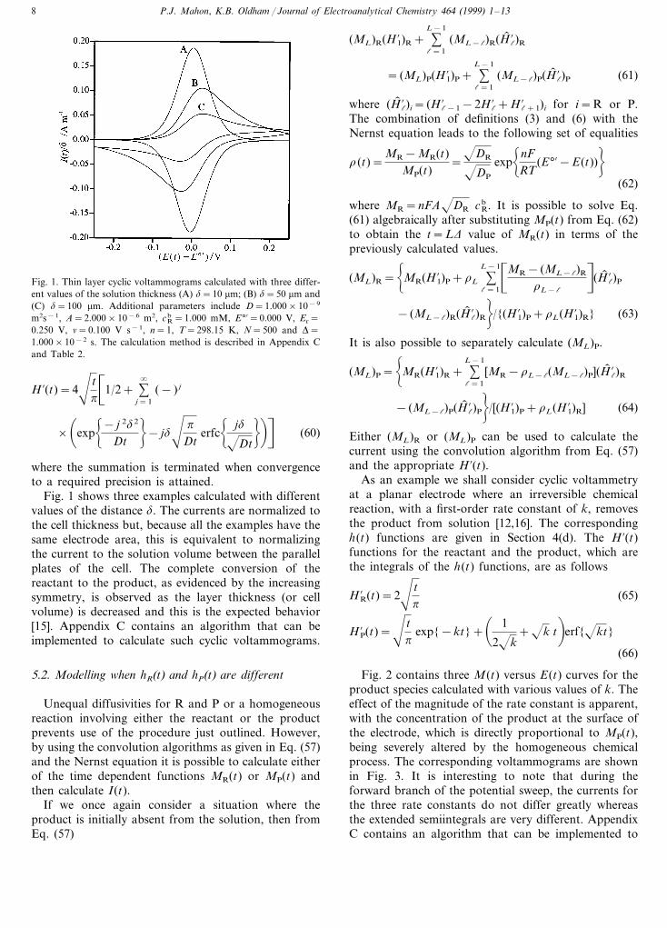
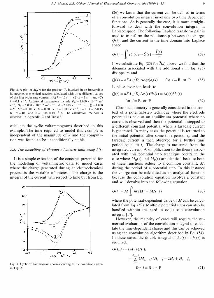
Fig. 2 contains three M(t) versus E(t) curves for theproduct species calculated with various values of k. Theeffect of the magnitude of the rate constant is apparent,with the concentration of the product at the surface ofthe electrode, which is directly proportional to MP(t),being severely altered by the homogeneous chemicalprocess. The corresponding voltammograms are shownin Fig. 3. It is interesting to note that during theforward branch of the potential sweep, the currents forthe three rate constants do not differ greatly whereasthe extended semiintegrals are very different. AppendixC contains an algorithm that can be implemented to

H %(t)=4' t

p

�1/2+ %

�

j=1

(− ) j

×�

exp!− j 2d2

Dt"

− jd' p

Dterfc

! jd

Dt

"�n(60)

where the summation is terminated when convergenceto a required precision is attained.

Fig. 1 shows three examples calculated with differentvalues of the distance d. The currents are normalized tothe cell thickness but, because all the examples have thesame electrode area, this is equivalent to normalizingthe current to the solution volume between the parallelplates of the cell. The complete conversion of thereactant to the product, as evidenced by the increasingsymmetry, is observed as the layer thickness (or cellvolume) is decreased and this is the expected behavior[15]. Appendix C contains an algorithm that can beimplemented to calculate such cyclic voltammograms.

5.2. Modelling when hR(t) and hP(t) are different

Unequal diffusivities for R and P or a homogeneousreaction involving either the reactant or the productprevents use of the procedure just outlined. However,by using the convolution algorithms as given in Eq. (57)and the Nernst equation it is possible to calculate eitherof the time dependent functions MR(t) or MP(t) andthen calculate I(t).

If we once again consider a situation where theproduct is initially absent from the solution, then fromEq. (57)


Fig. 2. A plot of MP(t) for the product, P, involved in an irreversiblehomogeneous chemical reaction calculated with three different valuesof the first order rate constant (A) k=10 s−1; (B) k=1 s−1 and (C)k=0.1 s−1. Additional parameters include DR=1.000×10−9 m2

s−1, DP=5.000×10−10 m2 s−1, A=2.000×10−6 m2, cbR=1.000

mM, E°%=0.000 V, Er=0.200 V, n=1.000 V s−1, n=1, T=298.15K, N=400 and D=1.000×10−3 s. The calculation method isdescribed in Appendix C and Table 3.

(26) we know that the current can be defined in termsof a convolution integral involving two time dependentfunctions. As is generally the case, it is more straight-forward to deal with the convolution integral inLaplace space. The following Laplace transform pair isused to transform the relationship between the charge,Q(t), and the current in the time domain into Laplacespace

Q(t)=& t

0

I(t)dtUQ( (s)=I( (s)

s(67)

If we substitute Eq. (25) for I(s) above, we find that thedilemma associated with the additional s in Eq. (25)disappears and

Q( (s)=nFADi Dci(s)h( i(s) for i=R or P (68)

Laplace inversion leads to

Q(t)=nFADi Dci(t)*hi(t)=Mi(t)*hi(t)

for i=R or P (69)

Chronocoulometry is generally considered in the con-text of a potential-step technique where the electrodepotential is held at an equilibrium potential where nocurrent is observed and then the potential is stepped toa different constant potential where a faradaic currentis generated. In many cases the potential is returned tothe initial potential after some time period, ts, and thefaradaic current is then observed for a further timeperiod equal to ts. The charge is measured from theintegrated current. A simplification to the theory associ-ated with this potential step technique occurs in thecase where MR(t) and MP(t) are identical because bothof these functions reduce to a common constant, M,during the period of a potential step. In this instancethe charge can be calculated as an analytical functionbecause the convolution equation involves a constantand will devolve into the following equation

Q(t)=M& t

0

h(t)dt=MH %(t) (70)

where the potential-dependent value of M can be calcu-lated from Eq. (59). Multiple potential steps can also behandled without the need to evaluate a convolutionintegral [17].

However, the majority of cases will require the nu-merical evaluation of the convolution integral to calcu-late the time-dependent charge and this can be achievedusing the convolution algorithm described in Eq. (54).In these cases, the double integral of hR(t) or hP(t) isrequired.

Q(LD)= (ML)i(H1)i

+ %L−1

l=1

(ML−l)i(Hl−1−2Hl+Hl+1)i

for i=R or P (71)

calculate the cyclic voltammograms described in thisexample. The time required to model this example isindependent of the magnitude of k and the computa-tion was found to be unconditionally stable.

5.3. The modelling of chronocoulometric data using h(t)

It is a simple extension of the concepts presented forthe modelling of voltammetric data to model caseswhere the charge generated during an electrochemicalprocess is the variable of interest. The charge is theintegral of the current with respect to time but from Eq.

Fig. 3. Cyclic voltammograms corresponding to the conditions givenin Fig. 2.


Fig. 4. A plot of MR(t) for the reactant and MP(t) for the productinvolved in an irreversible homogeneous chemical reaction calculatedwith three different values of the first order rate constant (A) k=10s−1; (B) k=1 s−1 and (C) k=0.1 s−1. Additional parametersinclude DR=DP=1.000×10−9 m2s−1, A=2.000×10−6 m2, cb

R=1.000 mM, E°%=0.000 V, Ei= −0.250 V, Es=0.250 V, n=1, T=298.15 K, N=500, ts=0.500 s and D=1.000×10−3 s. Thecalculation method is described in Appendix C and Table 4.

Fig. 5. Chronoamperograms corresponding to the conditions given inFig. 4.

Fig. 6. Chronocoulograms corresponding to the conditions given inFig. 4.

where HL=H(LD) and H(t)=t0 t

0 h(t) dt. Onceagain it will be necessary to calculate MR(t) or MP(t)before Q(t) is found and Eq. (63) or Eq. (64) can beused for this purpose, recalling that the single integralsof hR(t) and hP(t) are required.

As an example we will consider the reaction schemedescribed in the previous example except under doublepotential step conditions. The appropriate h(t) func-tions are from Section 4(d) and the single integrals aregiven in Eqs. (65) and (66). Either of the followingdouble integrals is required to calculate Q(t).

HR(t)=4t3/2

3p(72)

HP(t)=� t3/2

2p+

t

4kp

�exp{−kt}

+�k t2

2+

t

2k−

18k3/2

�erf{kt} (73)

The principles for this particular case are well estab-lished [18–21] and it therefore qualifies as an excellentexample to demonstrate modelling using the convolu-tion algorithm. Fig. 4 shows how MR(t) and MP(t) varyin response to the applied potential and the magnitudeof the homogeneous rate constant. It is once againobvious that an increasing amount of product is irre-versibly converted as the rate increases. However, inthis case, neither I(t) in Fig. 5 nor Q(t) in Fig. 6 areaffected by the homogeneous kinetics during the timeperiod where a substantial amount of the product isgenerated electrochemically. When the potential is re-

turned to its initial value, the current is diminished byan increase in k because the homogeneous chemicalprocess has lowered the concentration of the product,as expected. Appendix C contains an algorithm thatcan be implemented to calculate the chronocoulogramsdescribed in this example.

6. Conclusions

The derivation of Eq. (9) from a consideration of thefundamental diffusion process has established that theconvolution integral commonly encountered in the so-lution of electrochemical problems will always be appli-cable if the electrode has a shape that allows uniformaccessibility or if the electrochemical reaction is re-versible. In these cases, the functions g(t) and h(t) will


reflect the geometry of the electrode and the presence ofany homogeneous chemical reaction. In all other casesthe spatial complexity prevents the electrochemical sys-tem from being described by a combination of thetime-dependent functions I(t), M(t), g(t) and h(t).

We have also demonstrated that a pair of conjugatefunctions, g(t) and h(t), exists which enables the cur-rent and the surface concentrations to be interconvertedvia a convolution. Additionally, voltammetric andchronocoulometric modelling using h(t) and a convolu-tion algorithm was demonstrated. The advantage ofthis modelling method results from the incorporation ofthe spatial component of the diffusion problem into thetemporal function h(t). The h(t) functions may involvethe so-called special functions but this is not an imped-iment to the implementation of the convolution al-gorithm because these functions are now commonlyfound in mathematical computer packages such asMathematica® and Maple V®, which also contain so-phisticated programming and graphic capabilities.When the h(t) functions are not complicated, thestraightforward nature of the convolution algorithmwould enable many problems to be implemented withina spreadsheet environment.

Acknowledgements

The financial support of the Natural Sciences andEngineering Research Council of Canada is greatlyappreciated.

Appendix A

Without proof, we here present a result that will beuseful in Appendix B. When a step at the instant t=0takes the potential of a hemispherical electrode from anineffectual value to a constant value E at which theforward direction of reaction (1) has a heterogeneousrate constant kf, while kb is the corresponding back-ward rate constant, then the concentration of the ini-tially absent product P, at the electrode surface, obeysthe equation

cPs (t)=

� kfcRb

rDP

�×!DR

lm−

DR−rm

m(l−m)exp{m2t}erfc{mt}

−rl−DR

l(l−m)exp{l2t}erfc{lt}

"(A1)

Here r is the radius of the hemisphere, while l and m

are the solutions of the quadratic equation

Fig. 7. Diagram of the hybrid electrode.

s− (l+m)s+lm=0 (A2)

where

l+m=kf

DR

+kb

DP

+DR+DP

r(A3)

and

lm=DR DP

r�1

r+

kf

DR

+kb

DP

�(A4)

Both l and m are positive, with s−1/2 units; we select m

to represent the smaller of the pair. This result for aquasireversible potential step makes no assumptionabout the way in which the rate constants depend onpotential. See the literature [22] for the correspondingsolution for the current.

Appendix B

Symmetry arguments can be used to establish thatreactant and product concentrations will be uniform onthe surface of a suitably mounted planar, cylindrical,spherical or hemispherical electrode. Such geometriesare described as ‘uniformly accessible’. In this ap-pendix, we shall demonstrate by example that concen-trations on the surface of an electrode that is notuniformly accessible are sometimes close to beinguniform.

Fig. 7 diagrams an electrode that is not uniformlyaccessible but which is mathematically tractable. Itconsists of two hemispheres, of different radii, electri-cally connected. The hemispheres are sufficiently re-mote from each other to be diffusionally isolated. If apotential step is applied to the hybrid electrode, thenthe concentration of product at the surface of eachcomponent will be given by Eq. (A1). Only if thisequation predicts a lack of significant dependence ofc s

P(t) on r will the electrode behave in a manner suchthat the procedures of this article apply.

First consider the case when the forward rate con-stant is so large that the terms containing kf in Eqs.(A3) and (A4) totally dominate their congeners. Thenl=kf/DR and m=DP/r. In this circumstance, Eq.(A1) reduces to


cPs (t)cR

b ='DR

DP

−DR−DP

DP

exp!DPt

r2

"erfc

!DPtr

"−exp

!k f2t

DR

"erfc

!kf' t

DR

"(B1)

Note that r appears only in the second right-hand term,which is diminishing and small unless DP and DR areunusually disparate. Thus, the product concentration atthe surface of the hybrid electrode will be almost uni-form when kf dominates, i.e. at potentials commonlydescribed as ‘in the voltammetric plateau region’.This conclusion is independent of the degree of re-versibility of the electrode reaction. Though it has nobearing on our conclusion, note that, because of thelarge arguments of the exponential and complimentaryerror functions, the final term in Eq. (B1) rapidlyapproaches DR/(kfpt) and soon becomes negligible.

Next, we examine the reversible case in which kf andkb are both so large that only their ratio, given by theNernstian condition

kf

kb

=exp!nF

RT(E−E°%)

"=K (B2)

is significant. In these circumstances,

l=kf(DR+KDP)

DRDP

(B3)

and is very large, whereas

m=DR+KDP

r(DR+KDP)(B4)

has a value commensurate with Di/r. Substitution ofthese two expressions into Eq. (A1) yields the equation

cPs (t)cR

b =KDR

DR+KDP

−K2(DR−DP)DRDP

(DR+KDP)(DR+KDP)exp{m2t}erfc{mt}

−KDR

DR+KDP

exp{l2t}erfc{lt} (B5)

This equation displays an extremely complicated depen-dence of c s

P(t) on K and on the ratio of the diffusivities.Our present interest, however, is solely in the depen-dence on r and this enters Eq. (B5) only via m in thesecond right-hand term. Once more, the magnitude ofthis radius-dependent term is small and diminishing. Itis zero when the two diffusivities are equal, and negligi-ble otherwise, except at extremely small times. Weconclude that, for a reversible reaction, the concentra-tion of product on the surface of a hemisphere has noradius-dependence on and close to the voltammetricplateau, with a minor dependence elsewhere, whichdisappears as the two diffusivities attain similar values.

Now, let us address the general DR=DP case. Then,without approximation, l=D/r+k/D and m=

D/r, so that Eq. (A1) becomes

cPs (t)cR

b =kfr

D+kr�

1−exp!(D+kr)2t

r2D"

erfc!D+kr

r' t

D"n

(B6)

where k=kf+kb. This result shows that, in this equi-diffusivity case, all dependence on r vanishes whenk�D/r. Now, the minimum value of k is acquired atthe standard potential, and is 2k°, twice the standardrate constant. Hence, provided k° exceeds D/2r, therewill be negligible dependence of c s

P(t) on the radius r ofa hemispherical electrode, when both R and P share thesame diffusivity D.

We have shown that, for a potential step, the hybridelectrode of Fig. 7 mimics a uniformly–accessible elec-trode under certain circumstances. The mimicry is aidedby:� near equality of the diffusivities DR and DP;� a fast electrode reaction;� potentials on, or close to, the voltammetric plateau;� low electrode curvature;� prolonged electrolysis times.

These observations support the contentions made inSection 2. Of course, we cannot guarantee that similarconsiderations apply to non-uniformly–accessible elec-trodes of other geometries, or to other voltammetricmethods, but it seems reasonable to assume that such isthe case.

Appendix C

Generic algorithms for generating the cyclic voltam-mograms displayed in Sections 5.1 and 5.2 are pre-sented here, as is the algorithm needed to construct thechronocoulogram described in Section 5.3.

Each cyclic voltammogram is constructed from 2N+1 points, these being at the potentials

EL=E(LD)=Er− �L−N−1�6Dfor L=1, 2, … , 2N+1 (C1)

The initial (and final) potential, Er−NnD, is chosensuch that the initial current is negligible and Er is thereversal or switching potential.

The following steps are needed to create the voltam-mogram described in Section 5.1:

1. Input values of: RT/F, n, E°%, Er, nAFDR cbR,

d, N and D.2. Create storage, each of size 2N+1, for the

following arrays: EL, ML, H %L and IL.3–6. Then, in each case for L=1,2,…,2N+1, per-

form the calculations itemized in Table 2.7. Plot IL versus EL.


Table 2Four calculation steps, each calculated 2N+1 times, were needed tocalculate Fig. 1a

Step Calculate Equation

(C1)EL3(59)ML4

5 H %L (60)IL (57)6

a These were made sequentially, using the equations specified here.

Table 4Seven calculation steps, each calculated 2N times, were needed tocalculate Figs. 4–6a

EquationStep Calculate

3 rL (C2)(65)(H %L)R4

5 (66)(H %L)P

(HL)P (73)67 (ML)P (64)

IL (57)89 QL (71)

a These were made sequentially, using the equations specified here.Table 3Six calculation steps, each calculated 2N+1 times, were needed tocalculate Figs. 2 and 3a

CalculateStep Equation

(C1)EL3(62)rL4

(H %L)R5 (65)(H %L)P6 (66)

(64)(ML)P7(57)IL8

a These were made sequentially, using the equations specified here.

2. Create storage, each of size 2N, for arrays: rL,(H %L)R; (H %L)P; (HL)P; (ML)P; IL and QL.

3–9. Then, in each case for L=1, 2,…, 2N, per-form the calculations itemized in Table 4. In steps 7, 8and 9, a new (L−1)th-fold summation is needed foreach calculation.

10. Plot IL or QL versus LD.

References

[1] K.B. Oldham, Anal. Chem. 41 (1969) 1904.[2] M. Grenness, K.B. Oldham, Anal. Chem. 44 (1972) 1121.[3] K.B. Oldham, Anal. Chem. 58 (1986) 2296.[4] K.B. Oldham, J. Chem. Soc, Faraday Trans. I 82 (1986) 1099.[5] K.B. Oldham, J. Appl. Electrochem. 21 (1991) 1068.[6] C.P Andrieux, L. Nadjo, J.M. Saveant, J. Electroanal. Chem. 26

(1970) 147.[7] J.C. Imbeaux, J.M. Saveant, J. Electroanal. Chem. 44 (1973) 1969.[8] M. Goto, D. Ishii, J. Electroanal. Chem. 61 (1975) 361.[9] P. Dalrymple, M. Goto, K.B. Oldham, Anal. Chem. 49 (1977)

1390.[10] H.L. Surprenant, T.H. Ridgway, C.N. Reilley, J. Electroanal.

Chem. 75 (1977) 125.[11] P.J. Mahon, K.B. Oldham, J. Electroanal. Chem. 445 (1998) 179.[12] F.E. Woodard, R.D. Goodin, P. Kinlen, Anal. Chem. 56 (1984)

1920.[13] J.C. Myland, K.B. Oldham, C.G. Zoski, J. Electroanal. Chem.

193 (1985) 3.[14] J. Spanier, K.B. Oldham, An Atlas of Functions, Hemisphere,

Springer–Verlag, Washington DC, 1987.[15] A.T. Hubbard, F.C. Anson, Electroanalytical Chemistry; a Series

of Advances, vol. 4, Dekker, NY, 1970, p. 129.[16] R.S. Nicholson, I. Shain, Anal. Chem. 36 (1964) 706.[17] A.J. Bard, L.R. Faulkner, Electrochemical Methods; Theory and

Applications, Chapter 5, Wiley, NY, 1980.[18] W.M. Schwarz, I. Shain, J. Phys. Chem. 69 (1965) 30.[19] W.M. Schwarz, I. Shain, J. Phys. Chem. 70 (1966) 345.[20] J.H. Christie, J. Electroanal. Chem. 13 (1967) 79.[21] W.V. Childs, J.T. Maloy, C.P. Keszthelyi, A.J. Bard, J. Elec-

trochem. Soc. 118 (1971) 874.[22] A.M. Bond, K.B. Oldham, J. Electroanal. Chem. 158 (1983) 193.

The following steps are needed to create the voltam-mogram described in Section 5.2:

1. Input values of: RT/F, n, E°%, Er, nAFDR cbR,

DP, k, N and D.2. Create storage, each of size 2N+1, for the

following arrays: EL ; rL ; (H %L)R; (H %L)P; (ML)P and IL.3–8. Then, in each case for L=1,2,…,2N+1, per-

form the calculations itemized in Table 3.9. Plot IL versus EL.The chronocoulogram is constructed of 2N points,

these being at potentials E(t) equal to Es or Ei accord-ing as tB ts or t\ ts. The corresponding r(t) can becalculated by the formula

rL=r(LD)

=DR

DP

exp! nF

2RT�

2E°%+Ei+Es

+�LD− ts(Ei−Es)�

LD− ts

n"for L=1, 2, …, 2N (C2)

The following steps are needed to create Fig. 5 or Fig.6.

1. Input values of: RT/F, ts, E°%, Ei, Es,nAFDR cb

R, DP, k, N and D.

.

Documents

Convolutive modelling of electrochemical processes based on the relationship between the current and the surface concentration