Convolutional Neural Networks (CNN)

By Prof. Seungchul Lee Industrial AI Lab http://isystems.unist.ac.kr/ POSTECH

Table of Contents

I. 1. Convolution on ImageI. 1.1. Convolution in 1DII. 1.2. Convolution in 2D

II. 2. Convolutional Neural Networks (CNN)I. 2.1. MotivationII. 2.2. Convolutional OperatorIII. 2.3. Nonlinear Activation FunctionIV. 2.4. PoolingV. 2.5. Inside the Convolution Layer

III. 3. Lab: CNN with TensorFlowI. 3.1. Import LibraryII. 3.2. Load MNIST DataIII. 3.3. Build a ModelIV. 3.4. Define a CNN's ShapeV. 3.5. Define Weights, Biases and NetworkVI. 3.6. Define Loss, Initializer and OptimizerVII. 3.7. Summary of ModelVIII. 3.8. Define ConfigurationIX. 3.9. OptimizationX. 3.10. Test

IV. 4. Deep Learning of Things

1. Convolution on Image

1.1. Convolution in 1D

In [1]:

%%html <center><iframe src="https://www.youtube.com/embed/Ma0YONjMZLI?rel=0" width="560" height="315" frameborder="0" allowfullscreen></iframe></center>

Visualization of Cross Correlation and Convolution with Matlab

1.2. Convolution in 2DFilter (or Kernel)

Modify or enhance an image by filteringFilter images to emphasize certain features or remove other featuresFiltering includes smoothing, sharpening and edge enhancementDiscrete convolution can be viewed as element-wise multiplication by a matrix

In [2]:

# Import libraries import numpy as np import matplotlib.pyplot as plt from scipy.misc import imread, imresize from scipy.signal import convolve2d from six.moves import cPickle

% matplotlib inline

In [3]:

# Import image input_image = cPickle.load(open('./image_files/lena.pkl', 'rb'))

# Edge filter image_filter = np.array([[-1, 0, 1] ,[-1, 0, 1] ,[-1, 0, 1]])

# Compute feature feature = convolve2d(input_image, image_filter, boundary='symm', mode='same')

In [4]:

# Plot fig = plt.figure(figsize=(10, 6)) ax1 = fig.add_subplot(1, 3, 1) ax1.imshow(input_image, 'gray') ax1.set_title('Input image (512 x 512)', fontsize=15) ax1.set_xticks([]) ax1.set_yticks([])

ax2 = fig.add_subplot(1, 3, 2) ax2.imshow(image_filter, 'gray') ax2.set_title('Image filter (3 x 3)', fontsize=15) ax2.set_xticks([]) ax2.set_yticks([])

ax3 = fig.add_subplot(1, 3, 3) ax3.imshow(feature, 'gray') ax3.set_title('Feature', fontsize=15) ax3.set_xticks([]) ax3.set_yticks([]) plt.show()

In [5]:

# Import image input_image = cPickle.load(open('./image_files/lena.pkl', 'rb'))

# Gaussian filter image_filter = 1/273*np.array([[1, 4, 7, 4, 1] ,[4, 16, 26, 16, 4] ,[7, 26, 41, 26, 7] ,[4, 16, 26, 16, 4] ,[1, 4, 7, 4, 1]])

image_filter = imresize(image_filter, [15, 15])

# Compute feature feature = convolve2d(input_image, image_filter, boundary='symm', mode='same')

In [6]:

# Plot fig = plt.figure(figsize=(10, 6)) ax1 = fig.add_subplot(1, 3, 1) ax1.imshow(input_image, 'gray') ax1.set_title('Input image (512 x 512)', fontsize=15) ax1.set_xticks([]) ax1.set_yticks([])

ax2 = fig.add_subplot(1, 3, 2) ax2.imshow(image_filter, 'gray') ax2.set_title('Image filter (15 x 15)', fontsize=15) ax2.set_xticks([]) ax2.set_yticks([])

ax3 = fig.add_subplot(1, 3, 3) ax3.imshow(feature, 'gray') ax3.set_title('Feature', fontsize=15) ax3.set_xticks([]) ax3.set_yticks([]) plt.show()

2. Convolutional Neural Networks (CNN)

2.1. Motivation The bird occupies a local area and looks the same in different parts of an image. We should construct neuralnetworks which exploit these properties.

Generic structure of neural networkdoes not seem the bestdid not make use of the fact that we are dealing with imagesno regularization

Locality: objects tend to have a local spatial supportfully-connected layer locally-connected layer

→

Translation invariance: object appearance is independent of locationWeight sharing: untis connected to different locations have the same weights

object size

Convolutional Neural Networks

Simply neural networks that use the convolution in place of general matrix multiplication in at leastone of their layersThe convolution can be interpreted as an element-wise matrix multiplication

2.2. Convolutional OperatorMatrix multiplication

Every output unit interacts with every interacts unit

Convolution

Local connectivityWeight sharingTypically have sparse interactions

2.3. Nonlinear Activation Function

2.4. PoolingCompute a maximum value in a sliding window (max pooling)

Reduce spatial resolution for faster computationAchieve invariance to local translation

Pooling size :

Max pooling introduces invariances

2 × 2

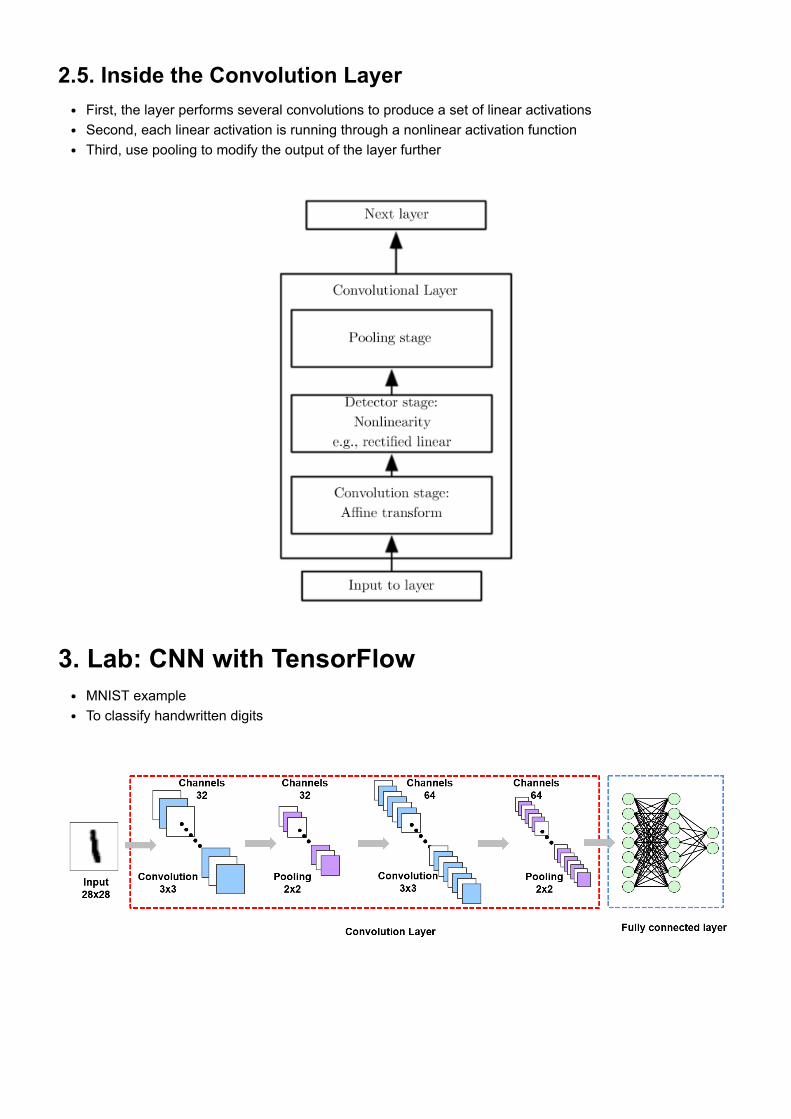
2.5. Inside the Convolution LayerFirst, the layer performs several convolutions to produce a set of linear activationsSecond, each linear activation is running through a nonlinear activation functionThird, use pooling to modify the output of the layer further

3. Lab: CNN with TensorFlowMNIST exampleTo classify handwritten digits

In [7]:

%%html <center><iframe src="https://www.youtube.com/embed/z6k_RMKExlQ?start=5150&end=6132?rel=0" width="560" height="315" frameborder="0" allowfullscreen></iframe></center>

ml4a @ itp nyu :: 03 convolutional neural networks

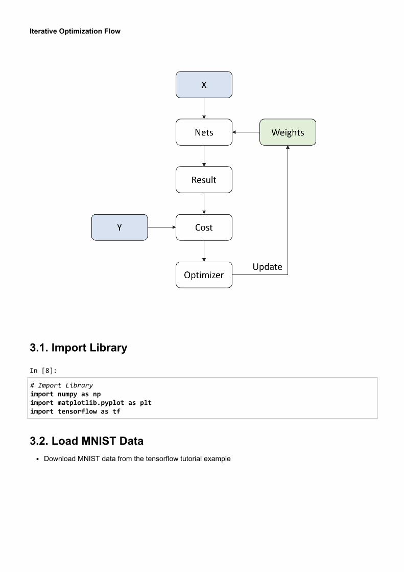
Iterative Optimization Flow

3.1. Import Library

In [8]:

# Import Library import numpy as np import matplotlib.pyplot as plt import tensorflow as tf

3.2. Load MNIST DataDownload MNIST data from the tensorflow tutorial example

In [9]:

from tensorflow.examples.tutorials.mnist import input_data mnist = input_data.read_data_sets("MNIST_data/", one_hot=True)

Extracting MNIST_data/train-images-idx3-ubyte.gz Extracting MNIST_data/train-labels-idx1-ubyte.gz Extracting MNIST_data/t10k-images-idx3-ubyte.gz Extracting MNIST_data/t10k-labels-idx1-ubyte.gz

In [10]:

# Check data train_x, train_y = mnist.train.next_batch(10) img = train_x[9,:].reshape(28, 28)

plt.figure(figsize=(5, 3)) plt.imshow(img,'gray') plt.title("Label : {}".format(np.argmax(train_y[9]))) plt.xticks([]) plt.yticks([]) plt.show()

3.3. Build a ModelConvolution layers

First, the layer performs several convolutions to produce a set of linear activationsSecond, each linear activation is running through a nonlinear activation functionThird, use pooling to modify the output of the layer further

Fully connected layers

Simple multi-layer perceptrons

First, the layer performs several convolutions to produce a set of linear activations

Filter size : Stride : The stride of the sliding window for each dimension of inputPadding : Allow us to control the kernel width and the size of the output independently

'SAME' : zero padding'VALID' : No padding

conv1 = tf.nn.conv2d(x, weights['conv1'], strides= [1,1,1,1], padding = 'SAME')

3 × 3

Second, each linear activation is running through a nonlinear activation function

conv1 = tf.nn.relu(tf.add(conv1, biases['conv1']))

Third, use a pooling to modify the output of the layer further

Compute a maximum value in a sliding window (max pooling)

Pooling size :

maxp1 = tf.nn.max_pool(conv1, ksize = [1, p1_h, p1_w, 1], strides = [1, p1_h, p1_w, 1], padding ='VALID')

2 × 2

Fully connected layer

Input is typically in a form of flattened featuresThen, apply softmax to multiclass classification problemsThe output of the softmax function is equivalent to a categorical probability distribution, it tells youthe probability that any of the classes are true.

output = tf.add(tf.matmul(hidden1, weights['output']), biases['output'])

3.4. Define a CNN's Shape

In [11]:

input_h = 28 # Input height input_w = 28 # Input width input_ch = 1 # Input channel : Gray scale # (None, 28, 28, 1)

## First convolution layer # Filter size k1_h = 3 k1_w = 3 # the number of channels k1_ch = 32 # Pooling size p1_h = 2 p1_w = 2 # (None, 14, 14 ,32)

## Second convolution layer # Filter size k2_h = 3 k2_w = 3 # the number of channels k2_ch = 64 # Pooling size p2_h = 2 p2_w = 2 # (None, 7, 7 ,64)

## Fully connected # Flatten the features # -> (None, 7*7*64) conv_result_size = int((28/(2*2)) * (28/(2*2)) * k2_ch) n_hidden1 = 100 n_output = 10

3.5. Define Weights, Biases and NetworkDefine parameters based on predefined layer sizeInitialize with normal distribution with and μ = 0 σ = 0.1

In [12]:

weights = { 'conv1' : tf.Variable(tf.random_normal([k1_h, k1_w, input_ch, k1_ch],stddev = 0.1

)), 'conv2' : tf.Variable(tf.random_normal([k2_h, k2_w, k1_ch, k2_ch],stddev = 0.1)), 'hidden1' : tf.Variable(tf.random_normal([conv_result_size, n_hidden1], stddev = 0.

1)), 'output' : tf.Variable(tf.random_normal([n_hidden1, n_output], stddev = 0.1))

}

biases = { 'conv1' : tf.Variable(tf.random_normal([k1_ch], stddev = 0.1)), 'conv2' : tf.Variable(tf.random_normal([k2_ch], stddev = 0.1)), 'hidden1' : tf.Variable(tf.random_normal([n_hidden1], stddev = 0.1)), 'output' : tf.Variable(tf.random_normal([n_output], stddev = 0.1))

}

x = tf.placeholder(tf.float32, [None, input_h, input_w, input_ch]) y = tf.placeholder(tf.float32, [None, n_output])

In [13]:

# Define Network def net(x, weights, biases): ## First convolution layer conv1 = tf.nn.conv2d(x, weights['conv1'], strides= [1, 1, 1, 1], padding = 'SAME') conv1 = tf.nn.relu(tf.add(conv1, biases['conv1'])) maxp1 = tf.nn.max_pool(conv1, ksize = [1, p1_h, p1_w, 1], strides = [1, p1_h, p1_w, 1], padding = 'VALID' ) ## Second convolution layer conv2 = tf.nn.conv2d(maxp1, weights['conv2'], strides= [1, 1, 1, 1], padding = 'SAME') conv2 = tf.nn.relu(tf.add(conv2, biases['conv2'])) maxp2 = tf.nn.max_pool(conv2, ksize = [1, p2_h, p2_w, 1], strides = [1, p2_h, p2_w, 1], padding = 'VALID')

# shape = conv2.get_shape().as_list() # maxp2_re = tf.reshape(conv2, [-1, shape[1]*shape[2]*shape[3]]) maxp2_re = tf.reshape(maxp2, [-1, conv_result_size]) ### Fully connected hidden1 = tf.add(tf.matmul(maxp2_re, weights['hidden1']), biases['hidden1']) hidden1 = tf.nn.relu(hidden1) output = tf.add(tf.matmul(hidden1, weights['output']), biases['output']) return output

3.6. Define Loss, Initializer and OptimizerLoss

Classification: Cross entropyEquivalent to apply logistic regression

Initializer

Initialize all the empty variables

Optimizer

GradientDescentOptimizerAdamOptimizer: the most popular optimizer

In [14]:

LR = 0.0001

pred = net(x, weights, biases) loss = tf.nn.softmax_cross_entropy_with_logits(labels=y, logits=pred) loss = tf.reduce_mean(loss)

# optimizer = tf.train.GradientDescentOptimizer(learning_rate).minimize(cost) optm = tf.train.AdamOptimizer(LR).minimize(loss)

init = tf.global_variables_initializer()

− log( ( )) + (1 − ) log(1 − ( ))1

N∑i=1

N

y(i) hθ x(i) y(i) hθ x(i)

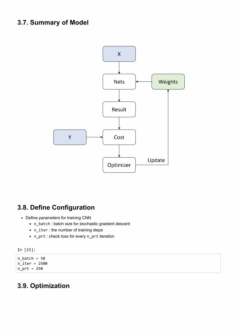
3.7. Summary of Model

3.8. Define ConfigurationDefine parameters for training CNN

n_batch : batch size for stochastic gradient descentn_iter : the number of training stepsn_prt : check loss for every n_prt iteration

In [15]:

n_batch = 50 n_iter = 2500 n_prt = 250

3.9. Optimization

In [16]:

# Run initialize # config = tf.ConfigProto(allow_soft_placement=True) # GPU Allocating policy # sess = tf.Session(config=config) sess = tf.Session() sess.run(init)

# Training cycle for epoch in range(n_iter): train_x, train_y = mnist.train.next_batch(n_batch) train_x = np.reshape(train_x, [-1, input_h, input_w, input_ch]) sess.run(optm, feed_dict={x: train_x, y: train_y}) if epoch % n_prt == 0: c = sess.run(loss, feed_dict={x: train_x, y: train_y}) print ("Iter : {}".format(epoch)) print ("Cost : {}".format(c))

Iter : 0 Cost : 2.8332996368408203 Iter : 250 Cost : 0.9441711902618408 Iter : 500 Cost : 0.30941206216812134 Iter : 750 Cost : 0.3349473476409912 Iter : 1000 Cost : 0.21016691625118256 Iter : 1250 Cost : 0.13401448726654053 Iter : 1500 Cost : 0.06568999588489532 Iter : 1750 Cost : 0.28441327810287476 Iter : 2000 Cost : 0.14654624462127686 Iter : 2250 Cost : 0.06276353448629379

3.10. Test

In [17]:

test_x, test_y = mnist.test.next_batch(100)

my_pred = sess.run(pred, feed_dict={x : test_x.reshape(-1, 28, 28, 1)}) my_pred = np.argmax(my_pred, axis=1)

labels = np.argmax(test_y, axis=1)

accr = np.mean(np.equal(my_pred, labels)) print("Accuracy : {}%".format(accr*100))

Accuracy : 99.0%

In [18]:

test_x, test_y = mnist.test.next_batch(1) logits = sess.run(tf.nn.softmax(pred), feed_dict={x : test_x.reshape(-1, 28, 28, 1)}) predict = np.argmax(logits)

plt.imshow(test_x.reshape(28, 28), 'gray') plt.xticks([]) plt.yticks([]) plt.show()

print('Prediction : {}'.format(predict))

plt.stem(logits.ravel()) plt.show()

np.set_printoptions(precision=2, suppress=True) print('Probability : {}'.format(logits.ravel()))

Prediction : 6

Probability : [ 0. 0. 0. 0. 0. 0. 1. 0. 0. 0.]

4. Deep Learning of ThingsCNN implemented in an Embedded System

In [19]:

%%html <center><iframe src="https://www.youtube.com/embed/baPLXhjslL8?rel=0" width="560" height="315" frameborder="0" allowfullscreen></iframe></center>

[iSystems] CNN in Raspberry Pi

In [20]:

%%javascript $.getScript('https://kmahelona.github.io/ipython_notebook_goodies/ipython_notebook_toc.js')