Andrea Vedaldi

Latest version of the slides http://www.robots.ox.ac.uk/~vedaldi/assets/teach/vedaldi16deepcv.pdf

Lab experiencehttps://www.robots.ox.ac.uk/~vgg/practicals/cnn-reg/

Convolutional Networks for

Computer Vision Applications

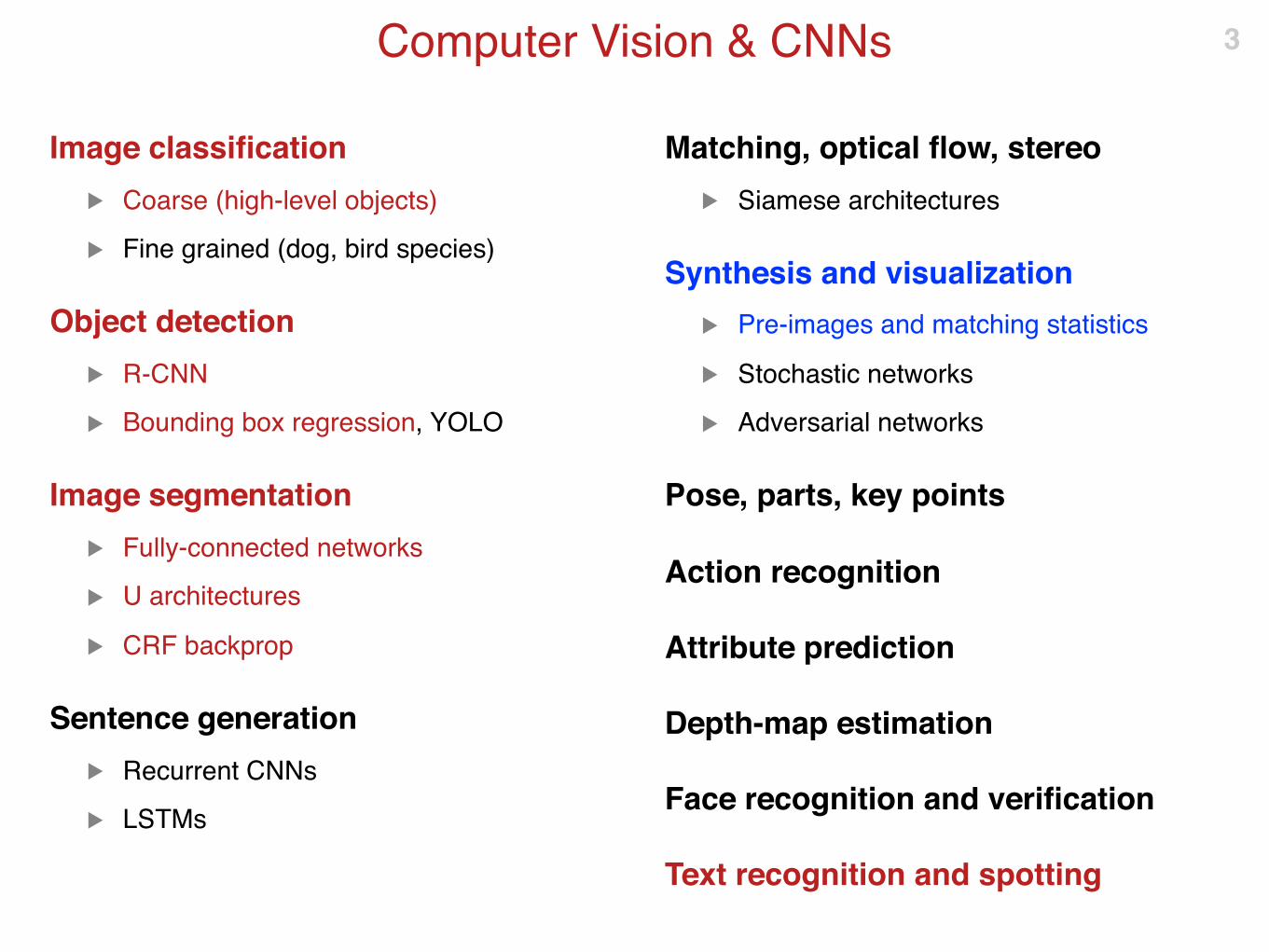
Computer Vision & CNNs

Image classification

▶ Coarse (high-level objects)

▶ Fine grained (dog, bird species)

Object detection

▶ R-CNN

▶ Bounding box regression, YOLO

Image segmentation

▶ Fully-connected networks

▶ U architectures

▶ CRF backprop

Sentence generation

▶ Recurrent CNNs

▶ LSTMs

Matching, optical flow, stereo

▶ Siamese architectures

Synthesis and visualization

▶ Pre-images and matching statistics

▶ Stochastic networks

▶ Adversarial networks

Pose, parts, key points

Action recognition

Attribute prediction

Depth-map estimation

Face recognition and verification

Text recognition and spotting

2

Computer Vision & CNNs

Image classification

▶ Coarse (high-level objects)

▶ Fine grained (dog, bird species)

Object detection

▶ R-CNN

▶ Bounding box regression, YOLO

Image segmentation

▶ Fully-connected networks

▶ U architectures

▶ CRF backprop

Sentence generation

▶ Recurrent CNNs

▶ LSTMs

Matching, optical flow, stereo

▶ Siamese architectures

Synthesis and visualization

▶ Pre-images and matching statistics

▶ Stochastic networks

▶ Adversarial networks

Pose, parts, key points

Action recognition

Attribute prediction

Depth-map estimation

Face recognition and verification

Text recognition and spotting

3

4

Review

c1 c2 c3 c4 c5 f6 f7 f8

w1 w2 w3 w4 w5 w6 w7 w8

bike

A. Krizhevsky, I. Sutskever, and G. E. Hinton. Imagenet classification with deep

convolutional neural networks. In Proc. NIPS, 2012.

A sequence of local & shift invariant layers

Convolutional Neural Network (CNN) 5

✱

Example: convolution layer

filter bank Finput data x output data y

There is a vector of feature channels (e.g. RGB) at each spatial location (pixel).

Data = 3D tensors 6

H

W

=

c = 1 c = 2 c = 3

channels

=3D tensor H

C

W

Each filter acts on multiple input channels

Convolution with 3D filters 7

Σ

x y

FLocalFilters look locally

Translation invariant Filters act the same everywhere

Multiple filters produce multiple output channels

Filter banks 8

One filter = one output channel

x

Σ

F(1)

Σ

F(2)

y

The basic blueprint of most architectures

Linear / non-linear chains 9

x

Σ

Σ

y

S

S

Σ S …

filtering ReLU filtering& downsampling

ReLU …

10

Three years of progress

From AlexNet (2012) to ResNet (2015)

How deep is enough? 11

AlexNet (2012)

5 convolutional layers

3 fully-connected layers

How deep is enough? 12

16 conv layers

AlexNet (2012) VGG-M (2013) VGG-VD-16 (2014)

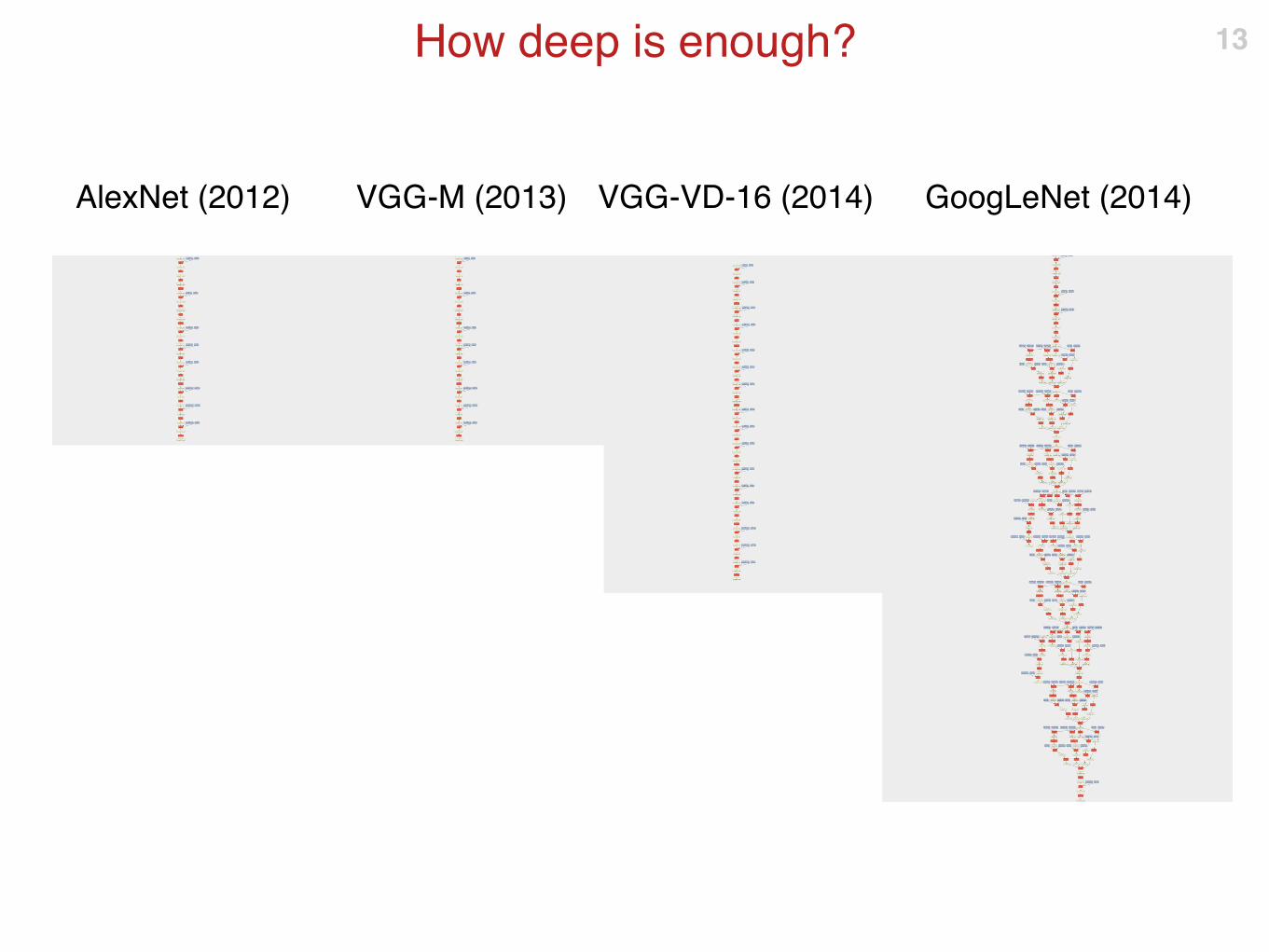
How deep is enough? 13

AlexNet (2012) VGG-M (2013) VGG-VD-16 (2014) GoogLeNet (2014)

How deep is enough? 14

AlexNet (2012) VGG-M (2013) VGG-VD-16 (2014) GoogLeNet (2014)

How deep is enough? 15

AlexNet (2012)

VGG-M (2013)

VGG-VD-16 (2014)

GoogLeNet (2014)

ResNet 152 (2015)

ResNet 50 (2015)

152 convolutional layers

50 convolutional layers

16 convolutional layers Krizhevsky, I. Sutskever, and G. E. Hinton.

ImageNet classification with deep convolutional

neural networks. In Proc. NIPS, 2012.

C. Szegedy, W. Liu, Y. Jia, P. Sermanet, S.

Reed, D. Anguelov, D. Erhan, V. Vanhoucke,

and A. Rabinovich. Going deeper with

convolutions. In Proc. CVPR, 2015.

K. Simonyan and A. Zisserman. Very deep

convolutional networks for large-scale image

recognition. In Proc. ICLR, 2015.

K. He, X. Zhang, S. Ren, and J. Sun. Deep

residual learning for image recognition. In Proc.

CVPR, 2016.

3 ⨉ more accurate in 3 years

Accuracy 16

To

p 5

err

or

0.0

2.5

5.0

7.5

10.0

12.5

15.0

17.5

20.0

caffe

-alex

vgg-f

vgg-m

googlenet-dag

vgg-ve

rydeep-1

6

resn

et-50-d

ag

resn

et-101-d

ag

resn

et-152-d

ag

Mo

re a

ccu

rate

0.0

0.3

0.7

1.0

1.3

1.6

2.0

2.3

2.6

caffe

-alex

vgg-f

vgg-m

googlenet-dag

vgg-ve

rydeep-1

6

resn

et-50-d

ag

resn

et-101-d

ag

resn

et-152-d

ag

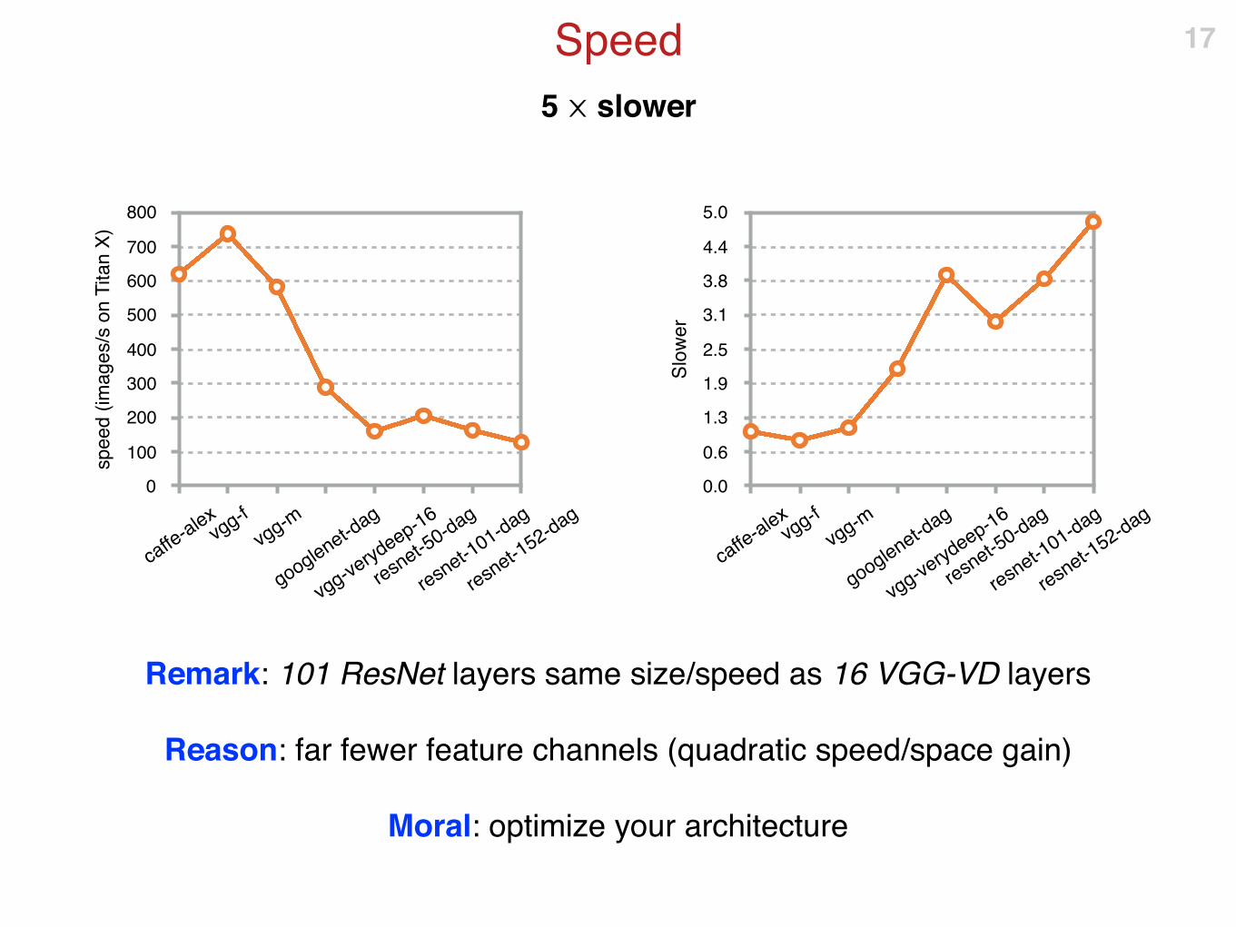
5 ⨉ slower

Speed

Remark: 101 ResNet layers same size/speed as 16 VGG-VD layers

Reason: far fewer feature channels (quadratic speed/space gain)

Moral: optimize your architecture

17

sp

ee

d (

ima

ge

s/s

on

Tita

n X

)

0

100

200

300

400

500

600

700

800

caffe

-alex

vgg-f

vgg-m

googlenet-dag

vgg-ve

rydeep-1

6

resn

et-50-d

ag

resn

et-101-d

ag

resn

et-152-d

ag

Slo

we

r

0.0

0.6

1.3

1.9

2.5

3.1

3.8

4.4

5.0

caffe

-alex

vgg-f

vgg-m

googlenet-dag

vgg-ve

rydeep-1

6

resn

et-50-d

ag

resn

et-101-d

ag

resn

et-152-d

ag

Num. of parameters is about the same

Model size 18

mo

de

l siz

e (

MB

s)

0

63

125

188

250

313

375

438

500

caffe

-alex

vgg-f

vgg-m

googlenet-dag

vgg-ve

rydeep-1

6

resn

et-50-d

ag

resn

et-101-d

ag

resn

et-152-d

ag

La

rge

r

0.0

0.8

1.5

2.3

3.0

3.8

4.5

5.3

6.0

caffe

-alex

vgg-f

vgg-m

googlenet-dag

vgg-ve

rydeep-1

6

resn

et-50-d

ag

resn

et-101-d

ag

resn

et-152-d

ag

Remark: 101 ResNet layers same size/speed as 16 VGG-VD layers

Reason: far fewer feature channels (quadratic speed/space gain)

Moral: optimize your architecture

Recent advances 19

Batch normalization

Design guidelines

Residual learning

Recent advances 20

Batch normalization

Design guidelines

Residual learning

From bottom to top

▶ The spatial resolution H ⨉ W decreases

▶ The number of channels C increases

Guideline

▶ Avoid tight information bottleneck

▶ Decrease the data volumeH ⨉ W ⨉ C slowly

Guideline 1: Avoid tight bottlenecks

Design guidelines 21

image

features

K. Simonyan and A. Zisserman. Very deep convolutional

networks for large-scale image recognition. In Proc.

ICLR, 2015.

C. Szegedy, V. Vanhoucke, S. Ioffe, and J. Shlens.

Rethinking the inception architecture for computer

vision. In Proc. CVPR, 2016.

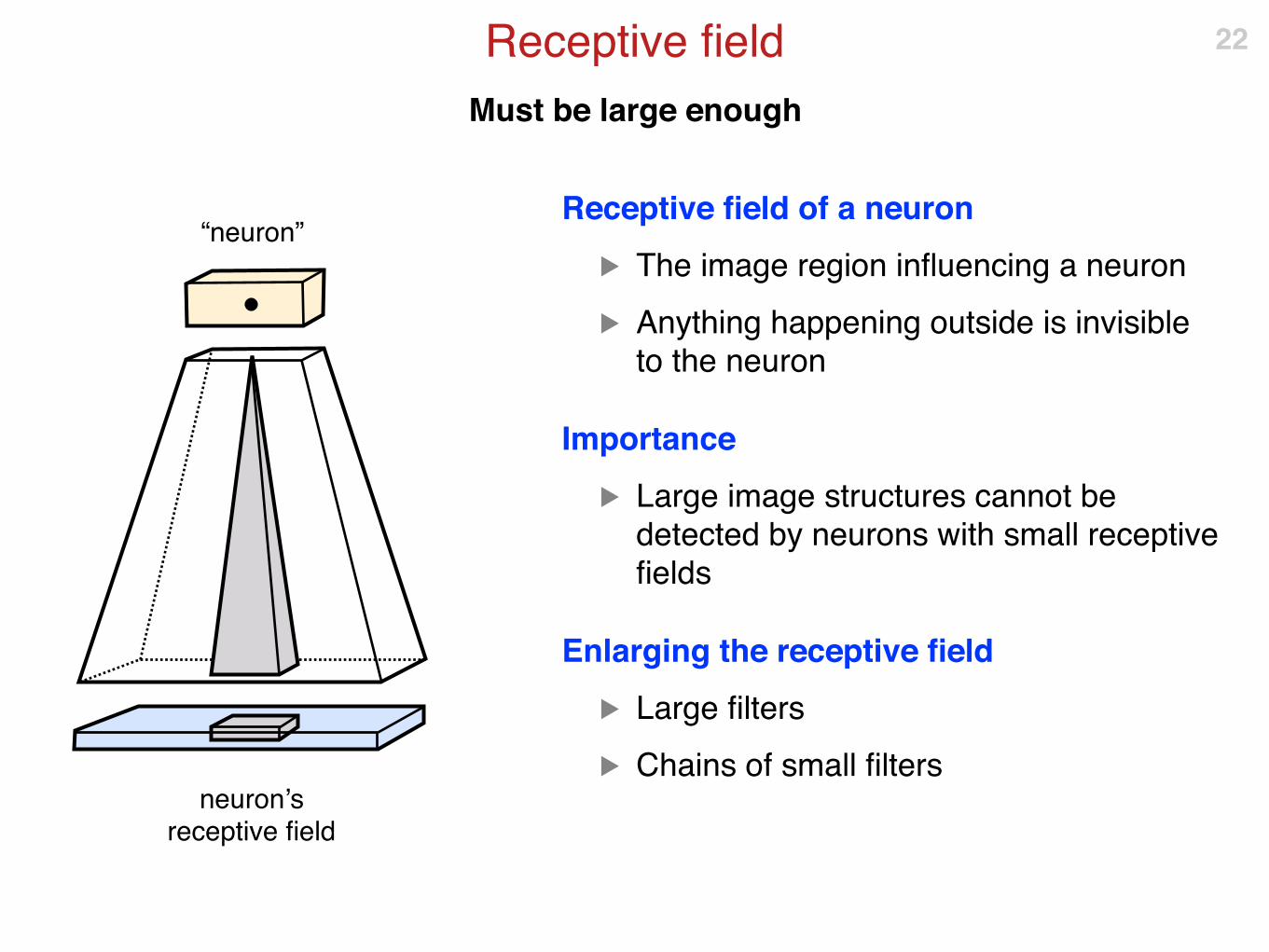
Must be large enough

Receptive field

Receptive field of a neuron

▶ The image region influencing a neuron

▶ Anything happening outside is invisible to the neuron

Importance

▶ Large image structures cannot be detected by neurons with small receptive fields

Enlarging the receptive field

▶ Large filters

▶ Chains of small filters

22

neuron’sreceptive field

“neuron”

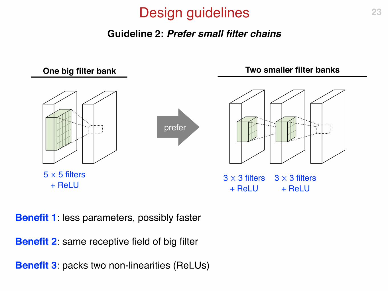
Guideline 2: Prefer small filter chains

Design guidelines

Benefit 1: less parameters, possibly faster

Benefit 2: same receptive field of big filter

Benefit 3: packs two non-linearities (ReLUs)

23

5 ⨉ 5 filters

+ ReLU3 ⨉ 3 filters

+ ReLU

prefer

3 ⨉ 3 filters

+ ReLU

One big filter bank Two smaller filter banks

Guideline 3: Keep the number of channels at bay

Design guidelines 24

H ⨉ W ⨉ C

Hf ⨉ Wf ⨉ C ⨉ K

C = num. input channels

K = num. output channels

Num. of operations

Num. of parameters

complexity ∝ C ⨉ K

Guideline 4: Less computations with filter groups

Design guidelines 25

split channels

filter groups

put back

M filters G groups of M/G filters

consider

instead

complexity ∝(C ⨉ K) / G

Guideline 4: Less computations with filter groups

Design guidelines

Groups = filters, seen as a matrix, have a “block” structure

26

⨉ =

xFy

⨉ =

xFy

0 0

0

00

0

complexity: C ⨉ K

C ⨉ K

complexity: C ⨉ K / G

Full filters Group-sparse filters

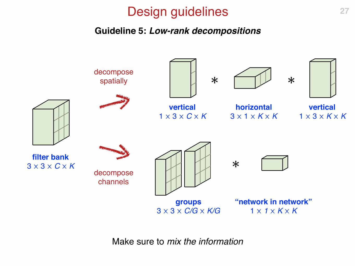
Guideline 5: Low-rank decompositions

Design guidelines

Make sure to mix the information

27

filter bank 3 ⨉ 3 ⨉ C ⨉ K

vertical1 ⨉ 3 ⨉ C ⨉ K

horizontal3 ⨉ 1 ⨉ K ⨉ K

vertical1 ⨉ 3 ⨉ K ⨉ K

groups 3 ⨉ 3 ⨉ C/G ⨉ K/G

“network in network” 1 ⨉ 1 ⨉ K ⨉ K

decompose spatially

decompose channels

✱ ✱

✱

Recent advances 28

Batch normalization

Design guidelines

Residual learning

Condition features

Batch normalization

Standardize the response of each feature channel within the batch

▶ Average over spatial locations

▶ Also, average over multiple images in the batch (e.g. 16-256)

29

batch ofN tensors

pick feature channel k

mean µk

variance σk

subtract mean &divide by variance

compute moments

S. Ioffe and C. Szegedy. Batch normalization: Accelerating deep network training by

reducing internal covariate shift. CoRR, 2015

Training vs testing modes

Batch normalization

Moments (mean & variance)

▶ Training: compute anew for each batch

▶ Testing: fixed to their average values

30

BN

x(3)

x(2)

x(1)

y(3)

y(2)

y(1)

momentsµ, σ

Training: batch-specificmoment averagesare collected

Testing:moment averages are used instead of batch-specific moments

Utilization

Batch normalization

Batch normalization is used after filtering, before ReLU

It is always followed by channel-specific scaling factor s and bias b

Noisy bias/variance estimation replaces dropout regularization

31

✱ BNscale bias

xn+3xn+1xn xn+2

ReLU

xn+4

momentsµ, σ

filters, biasesF, b

scale, biasess, b

Implemented a single block in

MatConvNet

Recent advances 32

Batch normalization

Design guidelines

Residual learning

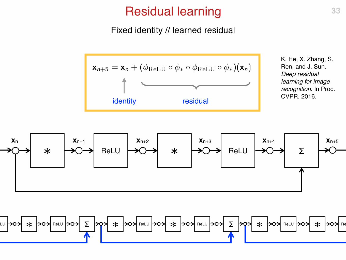
Fixed identity // learned residual

Residual learning 33

✱ ReLU ✱

xn+3xn+1xn xn+2

ReLU

xn+4

Σ

xn+5

identity residual

ReLU ✱ ReLU Σ ✱ ReLU ✱ ReLU Σ ✱ ReLU ✱ ReLU

K. He, X. Zhang, S.

Ren, and J. Sun.

Deep residual

learning for image

recognition. In Proc.

CVPR, 2016.

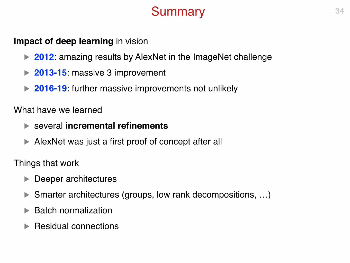
Summary

Impact of deep learning in vision

▶ 2012: amazing results by AlexNet in the ImageNet challenge

▶ 2013-15: massive 3 improvement

▶ 2016-19: further massive improvements not unlikely

What have we learned

▶ several incremental refinements

▶ AlexNet was just a first proof of concept after all

Things that work

▶ Deeper architectures

▶ Smarter architectures (groups, low rank decompositions, …)

▶ Batch normalization

▶ Residual connections

34

Semantic segmentation

Label individual pixels

Semantic image segmentation 36

c1 c2 c3 c4 c5 f6 f7 f8

input = image output = imageconvolutional fully-connected

Local receptive field

Convolutional layers 37

input image

features

receptive field

feature component

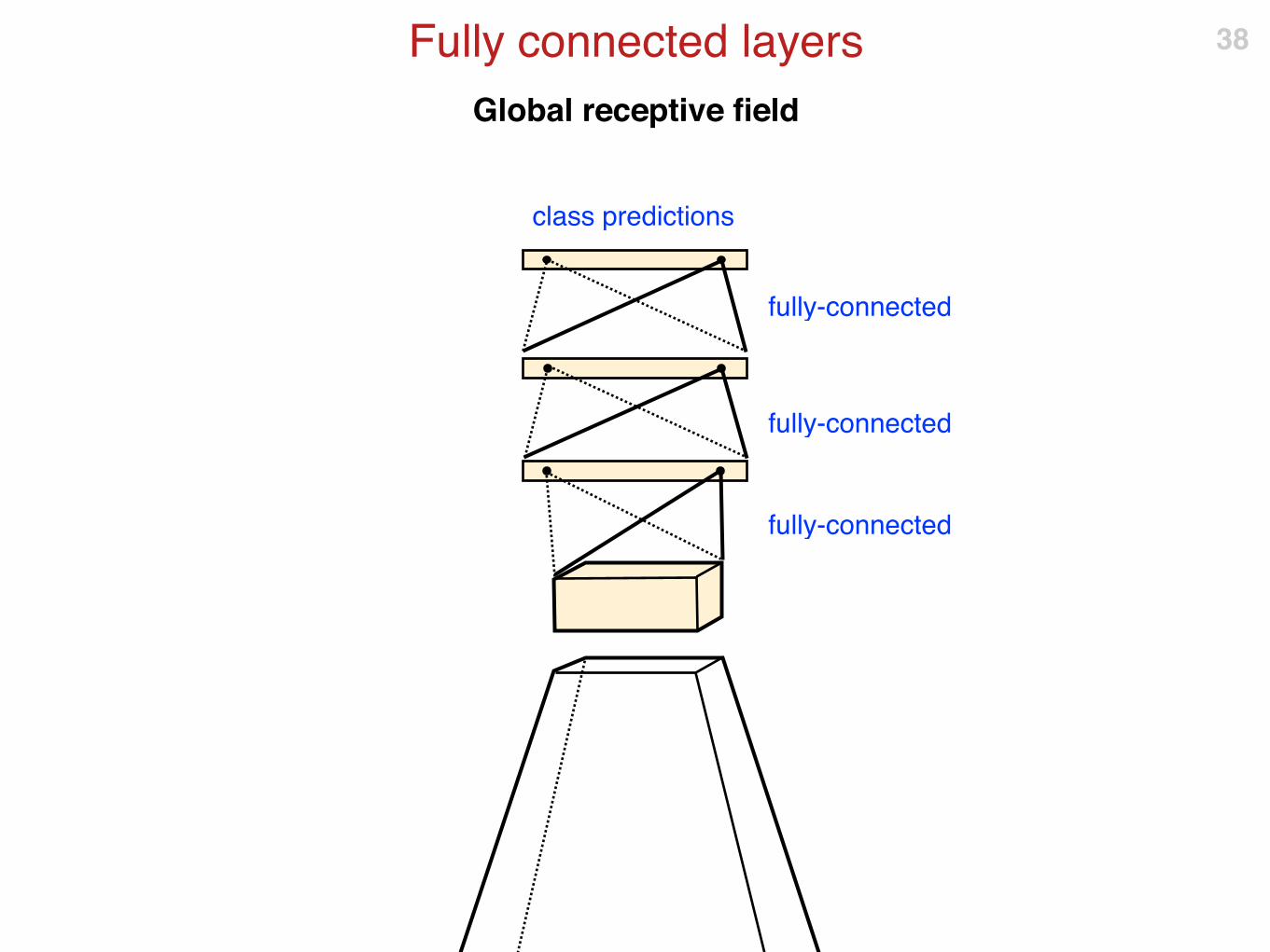
Global receptive field

Fully connected layers 38

fully-connected

class predictions

fully-connected

fully-connected

Comparing the receptive fields

Convolutional vs Fully Connected 39

Responses are spatially selective, can be used to localize things.

Responses are global, do not characterize well position

Which one ismore useful for

pixel level labelling?

Downsampling filters Upsampling filters

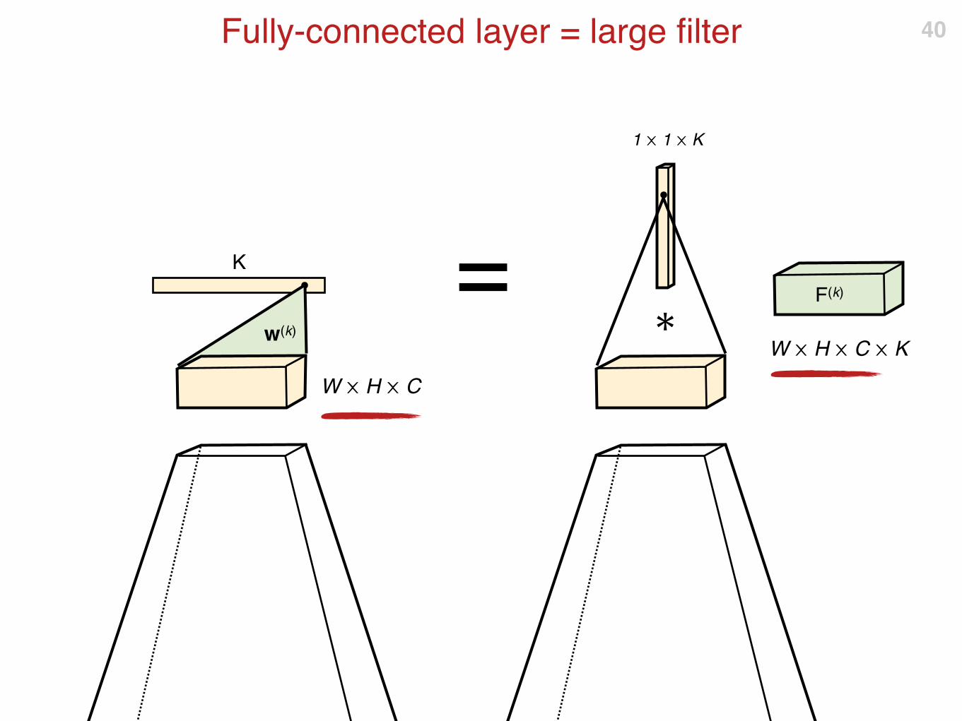
Fully-connected layer = large filter 40

F(k)

W ⨉ H ⨉ C

K

w(k)

W ⨉ H ⨉ C ⨉ K

1 ⨉ 1 ⨉ K

✱

=

Fully-convolutional neural networks 41

class predictions

J. Long, E. Shelhamer, and T. Darrell. Fully convolutional models for semantic segmentation. In Proc. CVPR, 2015

Fully-convolutional neural networks

Dense evaluation

▶ Apply the whole network convolutional

▶ Estimates a vector of class probabilities at each pixel

Downsampling

▶ In practice most network downsample the data fast

▶ The output is very low resolution (e.g. 1/32 of original)

42

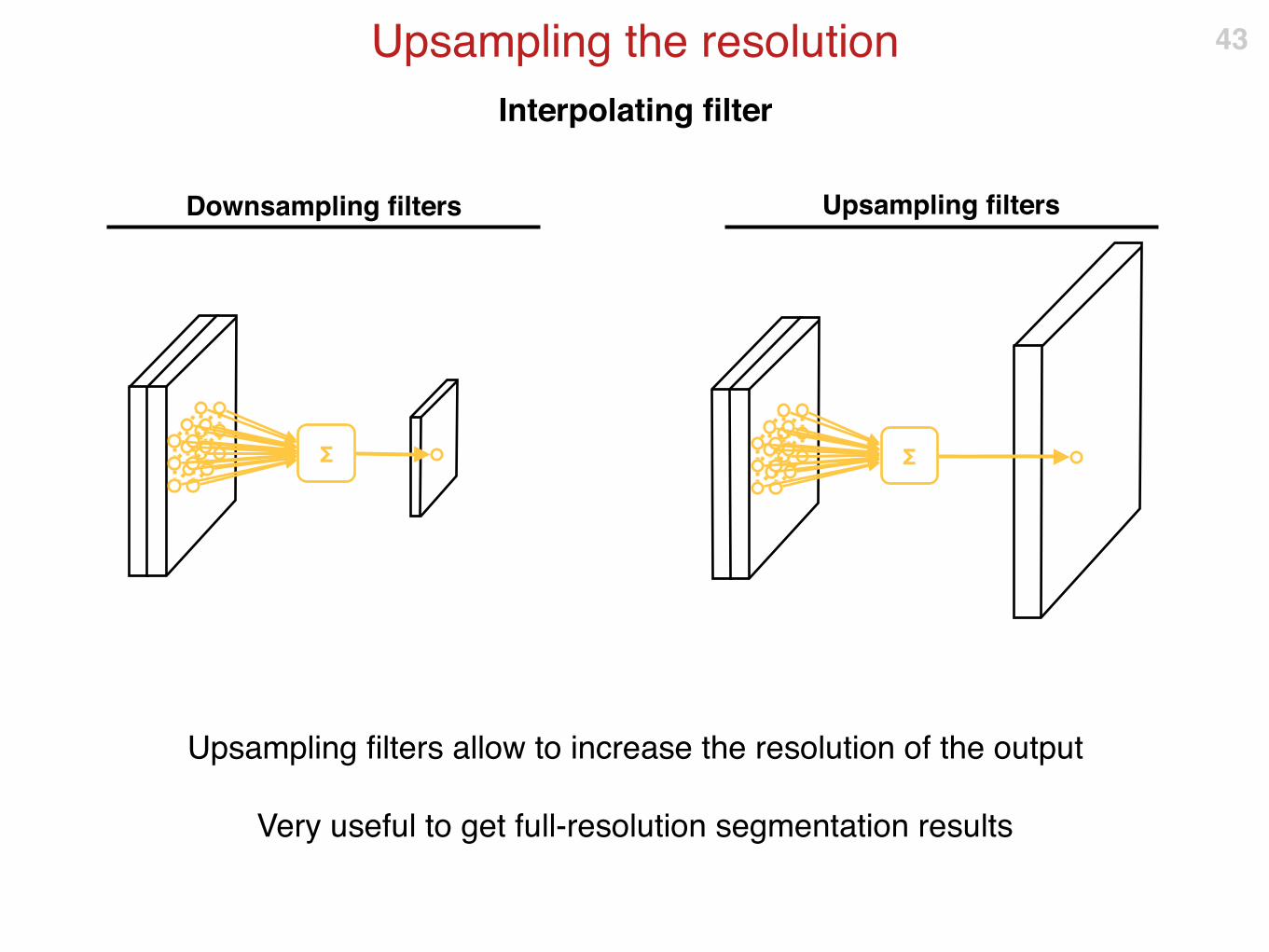
Interpolating filter

Upsampling the resolution

Upsampling filters allow to increase the resolution of the output

Very useful to get full-resolution segmentation results

43

Σ Σ

Downsampling filters Upsampling filters

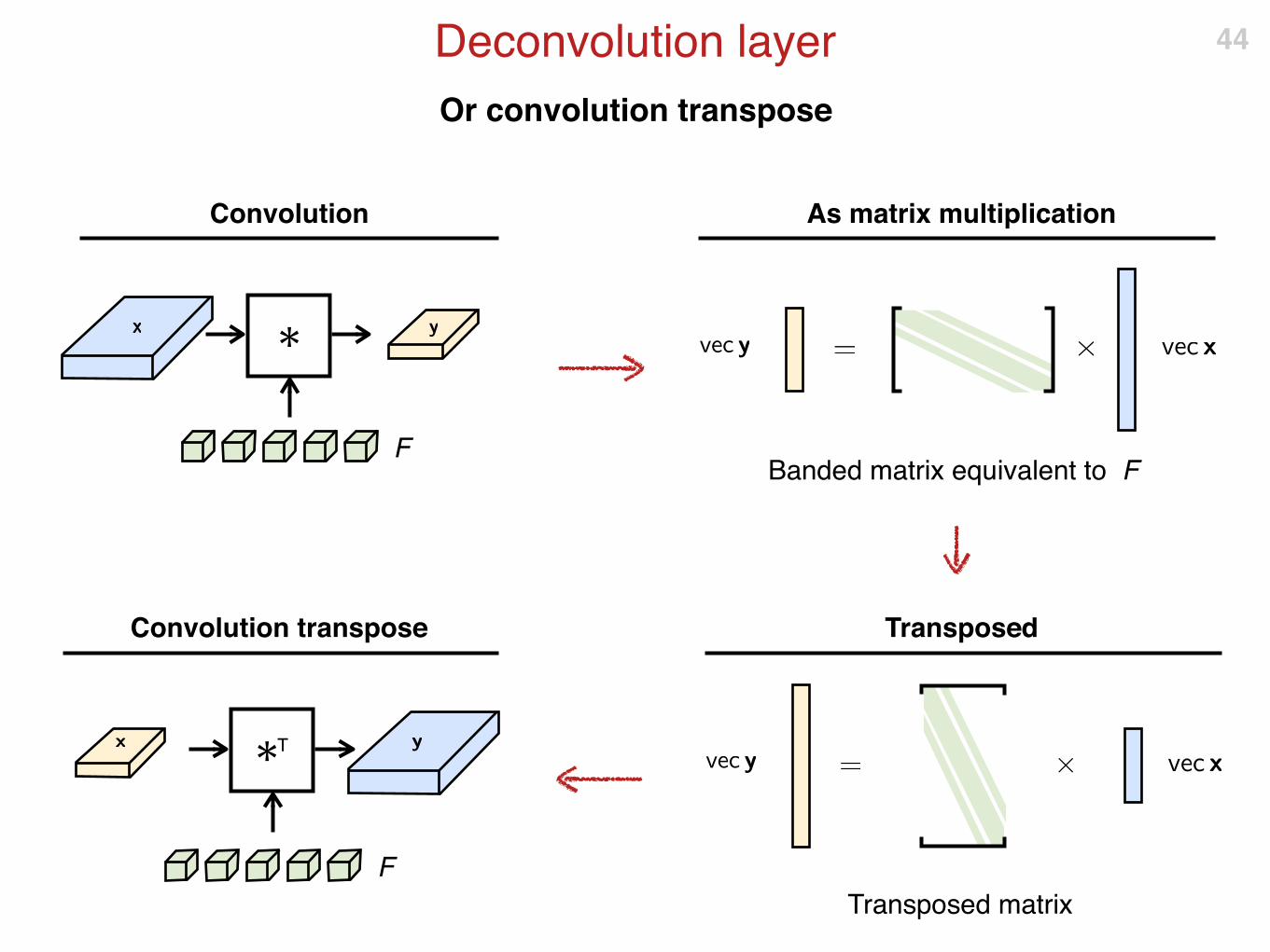
Or convolution transpose

Deconvolution layer 44

Convolution

✱

F

As matrix multiplication

Banded matrix equivalent to F

Transposed

Transposed matrix

Convolution transpose

✱T

F

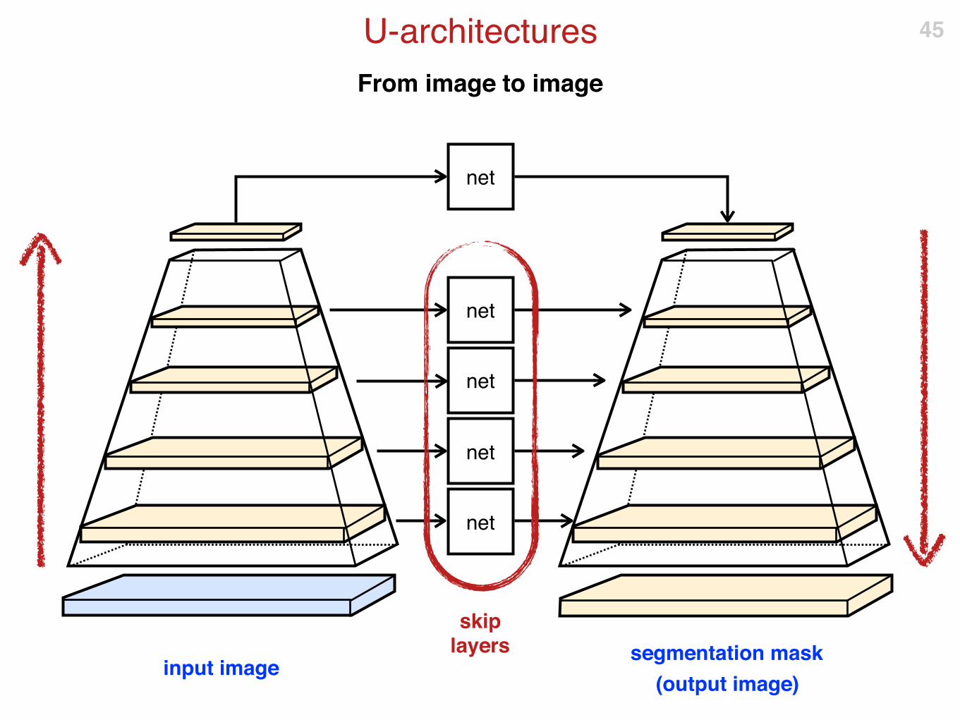
From image to image

U-architectures 45

input imagesegmentation mask

(output image)

net

net

net

net

net

skip layers

Several variants: FCN, U-arch, deconvolution, …

U-architectures 46

J. Long, E. Shelhamer, and T. Darrell. Fully convolutional models for semantic segmentation. In Proc. CVPR, 2015

H. Noh, S. Hong, and B. Han. Learning deconvolution network for semantic segmentation. In Proc. ICCV, 2015

O. Ronneberger, P. Fischer, and T. Brox. U-net: Convolutional networks for biomedical image segmentation. In Proc. MICCAI, 2015

copy and crop

inputimage

tile

output segmentation map

641

128

256

512

1024

max pool 2x2

up-conv 2x2

conv 3x3, ReLU

572

x 5

72

284²

64

128

256

512

57

0 x

570

568 x

568

28

2²

280

²1

40

²

13

8²

13

6²

68²

66

²

64

²3

2²

28²

56²

54²

52

²

512

104

²

10

2²

10

0²

200²

30²

19

8²

196²

392

x 3

92

39

0 x

390

38

8 x

38

8

388 x

388

1024

512 256

256 128

64128 64 2

conv 1x1

image pool4 pool5pool1 pool2 pool3

32x upsampled

prediction (FCN-32s)2x upsampled

prediction

16x upsampled

prediction (FCN-16s)

8x upsampled

prediction (FCN-8s)

pool4

prediction

2x upsampled

prediction

pool3

prediction

P P

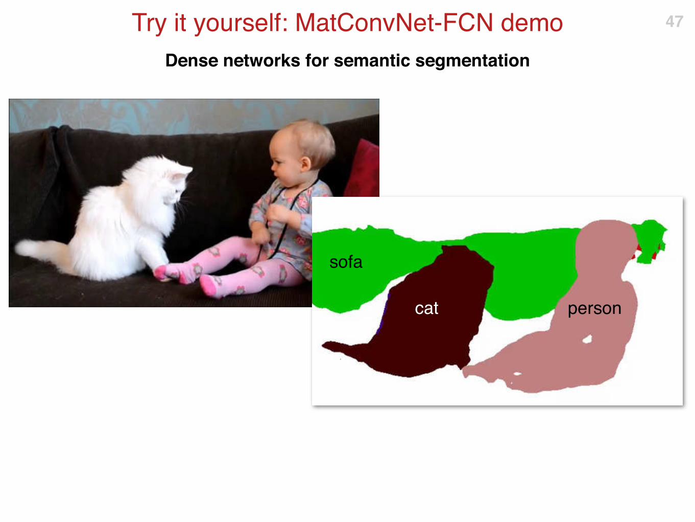
Dense networks for semantic segmentation

Try it yourself: MatConvNet-FCN demo 47

sofa

personcat

boat : 0.853 person :0.993

person :0.981

person :0.972

person :0.907

Object detection

Region-based Convolutional Neural Network

R-CNN

Pros: simple and effective

Cons: slow as the CNN is re-evaluated for each tested region

49

c5c1 c2 c3 c4 f6 f7 SVM label

Rich Feature Hierarchies for Accurate Object Detection and Semantic SegmentationR. Girshick, J. Donahue, T. Darrell, J. Malik, CVPR 2014

CNN chair

background

potted plant

CNN

CNN

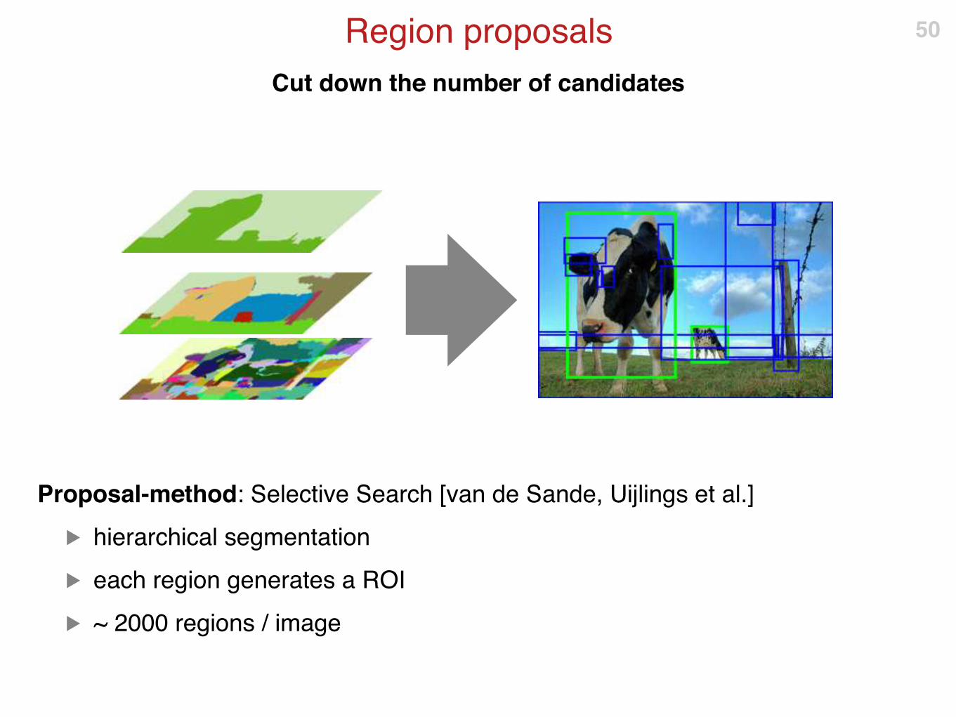
Cut down the number of candidates

Region proposals

Proposal-method: Selective Search [van de Sande, Uijlings et al.]

▶ hierarchical segmentation

▶ each region generates a ROI

▶ ~ 2000 regions / image

50

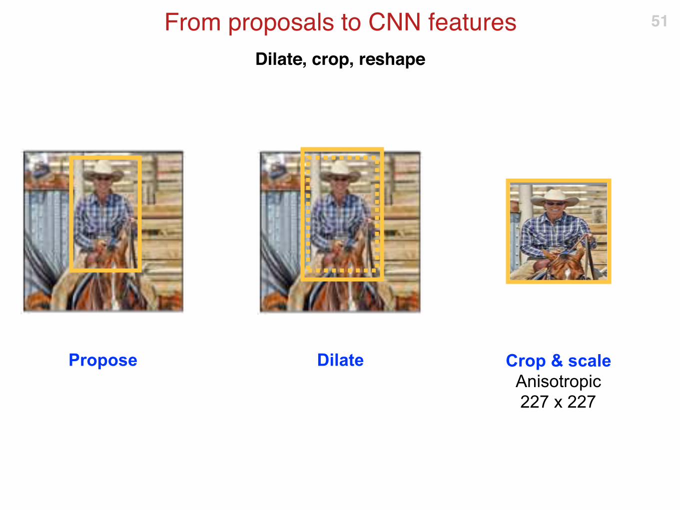
Dilate, crop, reshape

From proposals to CNN features 51

Dilate Crop & scale

Anisotropic

227 x 227

Propose

Evaluate CNN

From proposal to CNN features 52

Scale

Anisotropic

227 x 227

c5c1 c2 c3 c4 f6 f7

CNN features

Up to FC-7

AlexNet

Feature vector

4096 D

Run an SVM or similar on top

Classification of a region 53

Scale

Anisotropic

227 x 227

c5c1 c2 c3 c4 f6 f7

CNN features

Up to FC-7

AlexNet

Feature vector

4096 D

aeroplane

Label

One out of N

cat

dog

horse

person

…

SVM

old school

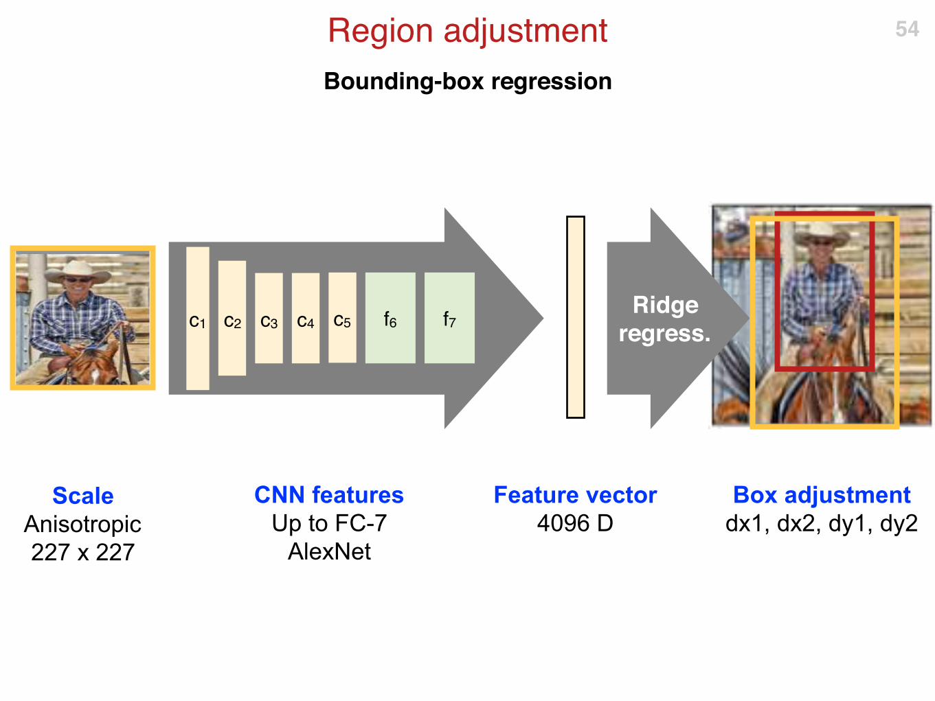
Bounding-box regression

Region adjustment 54

Scale

Anisotropic

227 x 227

c5c1 c2 c3 c4 f6 f7

CNN features

Up to FC-7

AlexNet

Feature vector

4096 D

Box adjustment

dx1, dx2, dy1, dy2

Ridge regress.

At the time of introduction (2013)

R-CNN results on PASCAL VOC 55

VOC 2007 VOC 2010

DPM v5 (Girshick et al. 2011) 33.7% 29.6%

UVA sel. search (Uijlings et al. 2013) 35.1%

Regionlets (Wang et al. 2013) 41.7% 39.7%

SegDPM (Fidler et al. 2013) 40.4%

R-CNN (TorontoNet) 54.2% 50.2%

R-CNN (TorontoNet) + bbox regression 58.5% 53.7%

R-CNN (VGG-VD) 62.1%

R-CNN (ONet) + bbox regression 66.0% 62.9%

Can we achieve end-to-end training?

Region-based Convolutional Neural Network

R-CNN summary 56

image

pertained on ImageNetthen fine-tuned

trained a-posterioriold school

Ridge regression

classimageSVM

classifierCNN

featuresRegion

proposals

box

End-to-end training

Except for region proposals

Problem: this is still pretty slow!

Region-based Convolutional Neural Network

Towards better R-CNNs 57

CNN regressor

classimageCNN

classifierCNN

featuresRegion

proposals

box

Accelerating R-CNN 58

c5c1 c2 c3 c4 f6 f7

c5c1 c2 c3 c4 f6 f7

c5c1 c2 c3 c4 f6 f7

chair

background

potted plant

crop

c5c1 c2 c3 c4

f6 f7

f6 f7

f6 f7

chair

background

potted plant

crop

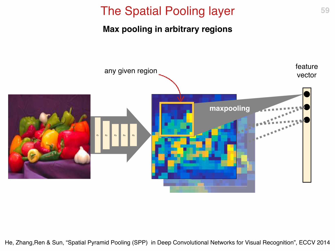
Max pooling in arbitrary regions

The Spatial Pooling layer 59

He, Zhang,Ren & Sun, “Spatial Pyramid Pooling (SPP) in Deep Convolutional Networks for Visual Recognition”, ECCV 2014

any given region

c5c1 c2 c3 c4

feature vector

maxpooling

As a building block

The Spatial Pooling layer 60

SPfeature

map

list ofregions

region-specificfeature vectors

He, Zhang,Ren & Sun, “Spatial Pyramid Pooling (SPP) in Deep Convolutional Networks for Visual Recognition”, ECCV 2014

Same as above, but for multiple subdivisions

The Spatially Pyramid Pooling Layer 61

maxpooling

Summary

Fast R-CNN 62

c5c1 c2 c3 c4

f6 f7 chair

selective search

SPPr6 r7 box refinement

f6 f7 background

r6 r7 box refinement

f6 f7 potted plant

r6 r7 box refinement

still not so fast

Ross Girshick. “Fast R-CNN”. ICCV 2015

same parameters

Fixed image-independent proposal set

R-CNN minus R

Fixed proposal generation

▶ Take all bounding box in the training set

▶ Run K-means clustering to distill a few thousands

63

[Lenc Vedaldi BMVC 2015]

all training boxes

simplifyusing clustering

~2-3000 representative boxes

Matches the training set statistics by construction

Vs other proposal sets 64

ground truthselective search

2Ksliding windows

7Kclustering

3K

Replace image-specific boxes with a fixed pool

R-CNN minus R 65

c5c1 c2 c3 c4

f6 f7 chair

SPPr6 r7 box refinement

f6 f7 background

r6 r7 box refinement

f6 f7 potted plant

r6 r7 box refinement

fixed boxes pool

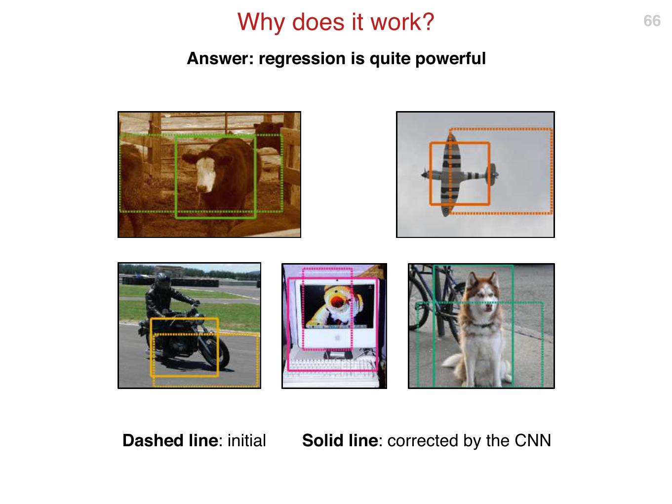
Answer: regression is quite powerful

Why does it work? 66

Dashed line: initial Solid line: corrected by the CNN

Image-specific vs fixed

Quantitative comparisons

Selective search is much better than fixed generators

However, bounding box regression almost eliminates the difference

Clustering allows to use significantly less boxes than sliding windows

67

mA

P (

VO

C0

7)

0.42

0.4675

0.515

0.5625

0.61

Sel. Search (2K boxes)

Slid. Win.(7K Boxes)

Clusters(2K Boxes)

Clusters(7K Boxes)

Baseline BBR

Even better performance with fixed proposals

Faster R-CNN

Ideas:

▶ Better fixed region proposal sampling

▶ Proposal shape specific classifier / regressors

68

Ren, He, Girshick, & Sun. “Faster R-CNN: Towards Real-Time Object Detection with Region Proposal Networks”. NIPS 2015.

3 s

ca

les

3 aspect ratios

proposalsprototypes(anchors)

together

Even better performance with fixed proposals

Faster R-CNN 69

Ren, He, Girshick, & Sun. “Faster R-CNN: Towards Real-Time Object Detection with Region Proposal Networks”. NIPS 2015.

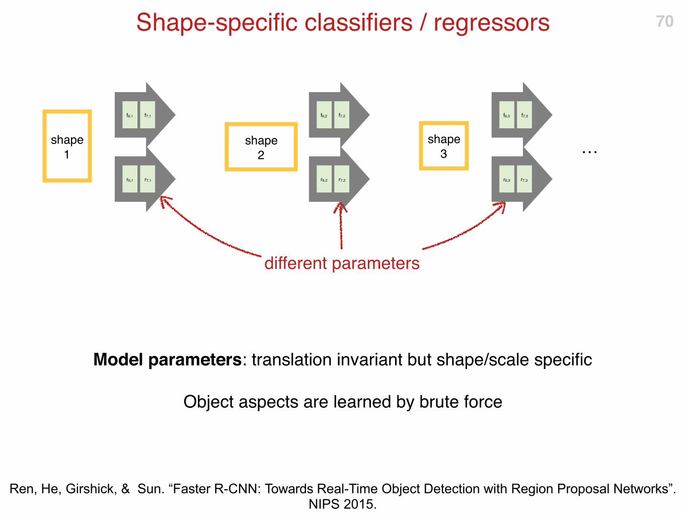
Shape-specific classifiers / regressors

Model parameters: translation invariant but shape/scale specific

Object aspects are learned by brute force

70

f6,1 f7,1

shape

1

r6,1 r7,1

f6,2 f7,2

r6,2 r7,2

shape

2

shape

3

f6,3 f7,3

r6,3 r7,3

…

different parameters

Ren, He, Girshick, & Sun. “Faster R-CNN: Towards Real-Time Object Detection with Region Proposal Networks”. NIPS 2015.

Based on overlap with ground truth

Training: what is a positive or negative box? 71

treat aspositive

overlap > 70%

treat asnegative

overlap < 30%

Ren, He, Girshick, & Sun. “Faster R-CNN: Towards Real-Time Object Detection with Region Proposal Networks”. NIPS 2015.

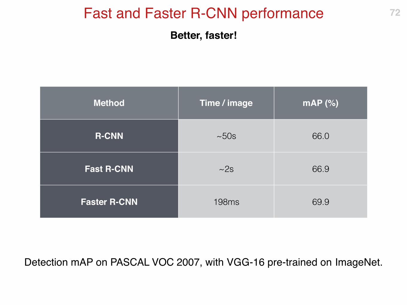
Better, faster!

Fast and Faster R-CNN performance 72

Method Time / image mAP (%)

R-CNN ~50s 66.0

Fast R-CNN ~2s 66.9

Faster R-CNN 198ms 69.9

Detection mAP on PASCAL VOC 2007, with VGG-16 pre-trained on ImageNet.

Three strategies

Multi-scale representations 73

scale image scale feature filters fixed scale features

model parameters shared for all scales

recompute features for each scale

cannot exploit fine details when visible

“brute force” modeling of scale

compute features at a single scale

can model fine details just fine

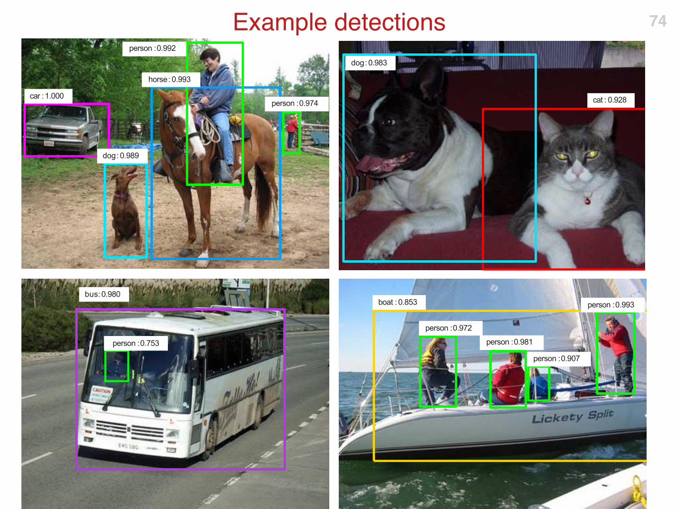
Example detections 74

bus: 0.980

car : 1.000

dog : 0.989

person : 0.992

person : 0.974

horse : 0.993

boat : 0.853 person : 0.993

person : 0.981

person : 0.972

person : 0.907

cat : 0.928

dog : 0.983

person : 0.753

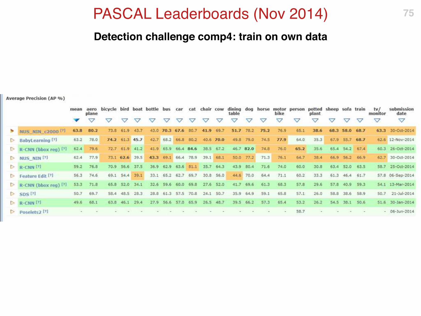
Detection challenge comp4: train on own data

PASCAL Leaderboards (Nov 2014) 75

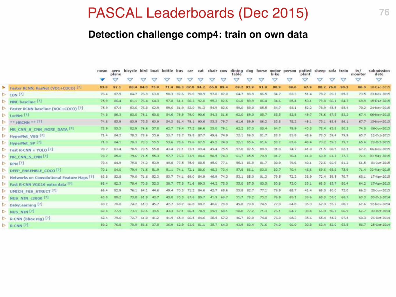
Detection challenge comp4: train on own data

PASCAL Leaderboards (Dec 2015) 76

Part II: A CNN example in text spotting1.00/1.00/1.00

LORD

NELSON

Other applications

Siamese networks for face recognition/verification

Huge variety of applications

E.g. VGG-Face

78

same different

Text spotting

Huge variety of applications

E.g. SynthText and VGG-Text

79

CREAM

http://zeus.robots.ox.ac.uk/textsearch/#/search/

A two-step approach

We will focus on the “classification” step

Most previous approaches start by recognising individual characters [Yao et al. 2014, Bissacco et al. 2013, Jaderberg et al. 2014, Posner et al. 2010, Quack et al. 2009, Wang et al. 2011, Wang et al. 2012, Weinman et al. 2014, …]

The alternative is to directly map word images to words [Almazan et al. 2014, Goel et al. 2013, Mishra et al. 2012, Novikova et al. 2012, Rodriguez-Serrano et al. 2012, Godfellow et al. 2013]

80

detection

“APARTMENTS”

classification

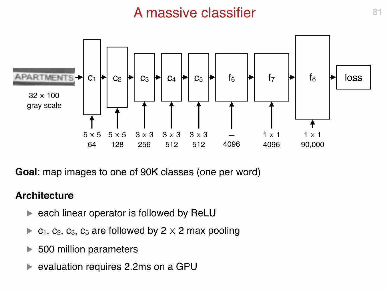
A massive classifier

Goal: map images to one of 90K classes (one per word)

Architecture

▶ each linear operator is followed by ReLU

▶ c1, c2, c3, c5 are followed by 2 ⨉ 2 max pooling

▶ 500 million parameters

▶ evaluation requires 2.2ms on a GPU

81

c1 c2 c3 c4 c5 f6 f7 f8 loss

5 ⨉ 5

64

5 ⨉ 5

128

3 ⨉ 3

256

3 ⨉ 3

512

3 ⨉ 3

512

—

4096

1 ⨉ 1

4096

1 ⨉ 1

90,000

32 ⨉ 100

gray scale

Learning a massive classifier

Massive training data 9 million images spanning 90K words (100 examples per word)

Learning algorithm

▶ SGD

▶ dropout (after fc6 and fc7)

▶ mini batches

Problem

▶ in practice each batch must contain at least 1/5 of all the classes

▶ batch size = 18K (!!)

Solution: incremental training

▶ learn first using 5K classes only (1K minibatches)

▶ then incrementally add 5K more classes

82

Synth Text dataset

Existing text recognition benchmark datasets are too small to train the model

Synth Text

▶ http://www.robots.ox.ac.uk/~vgg/data/text/

▶ a new synthetic dataset for text spotting

▶ include realistic visual effects

▶ infinity large (9M images available for download)

83

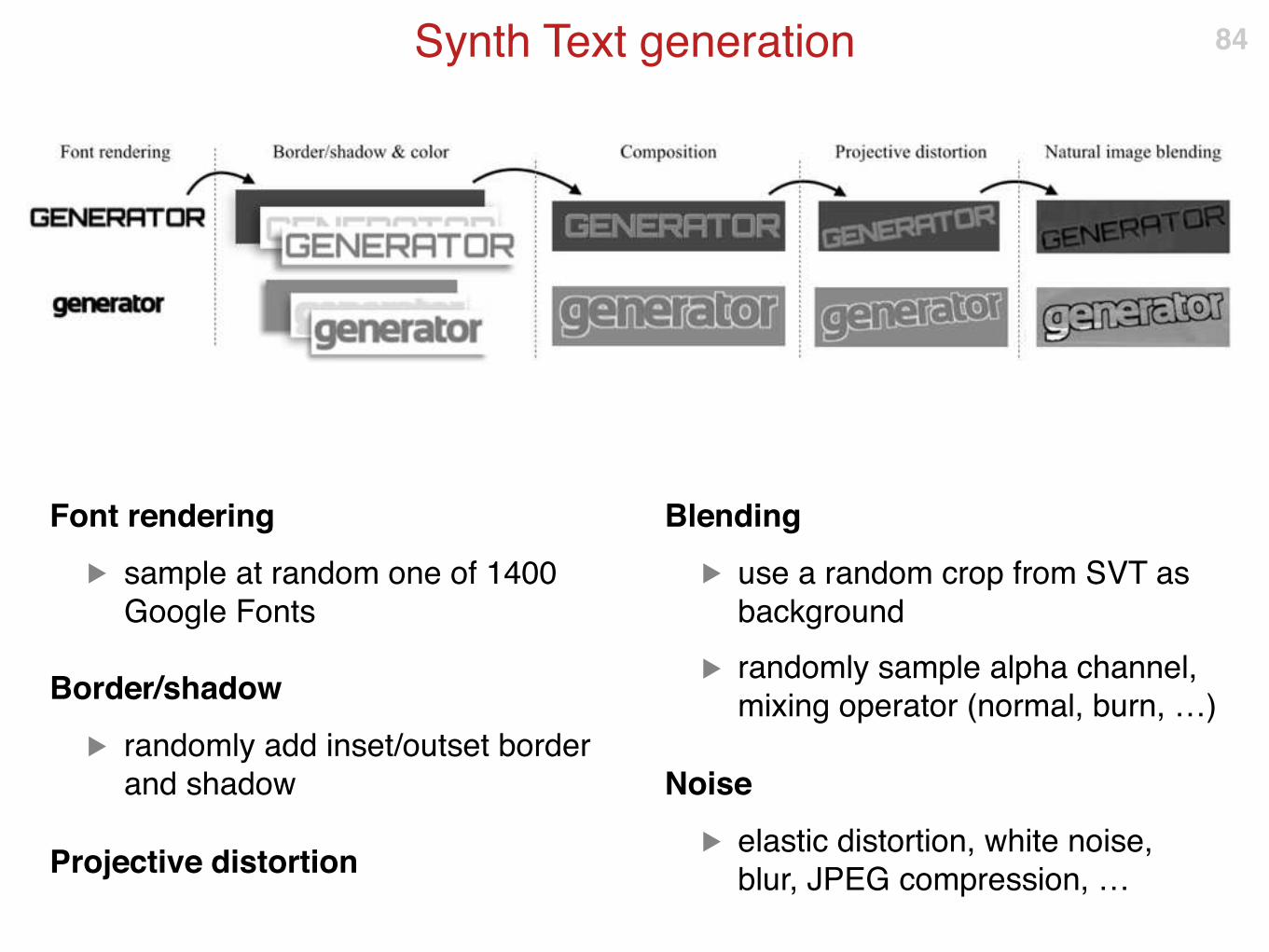
Synth Text generation

Font rendering

▶ sample at random one of 1400

Google Fonts

Border/shadow

▶ randomly add inset/outset border

and shadow

Projective distortion

Blending

▶ use a random crop from SVT as

background

▶ randomly sample alpha channel,

mixing operator (normal, burn, …)

Noise

▶ elastic distortion, white noise,

blur, JPEG compression, …

84

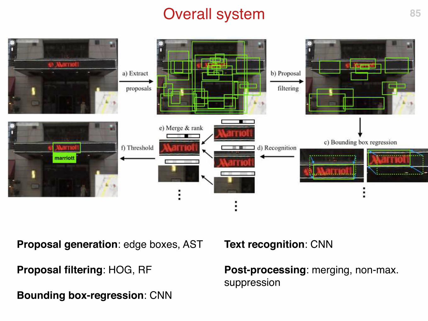
Overall system

Proposal generation: edge boxes, AST

Proposal filtering: HOG, RF

Bounding box-regression: CNN

Text recognition: CNN

Post-processing: merging, non-max.

suppression

85

Qualitative results: text spotting 86

1.00/1.00/1.001.00/1.00/1.00

1.00/1.00/1.00

1.00/1.00/1.00

Qualitative results: text spotting 87

1.00/1.00/1.001.00/0.88/0.93

1.00/1.00/1.00

1.00/1.00/1.00

Qualitative results: text retrieval 88

“APARTMENTS” “BORIS JOHNSON” “HOLLYWOOD”

Qualitative results: text retrieval 89

“POLICE” “CASTROL” “VISION”

Backpropagation revisited

Compute derivatives using the chain rule

Backpropagation 91

c1 c2 c3 c4 c5 f6 f7 f8 loss

bike

error

w1 w2 w3 w4 w5 w6 w7 w8

ℝx

forward

derror

dw1

derror

dw2

derror

dw3

derror

dw4

derror

dw5

derror

dw6

derror

dw7

derror

dw8

backward

Chain rule: scalar version 92

f1 f2 fn-1 fn

xnx1

…

x0 xn-1

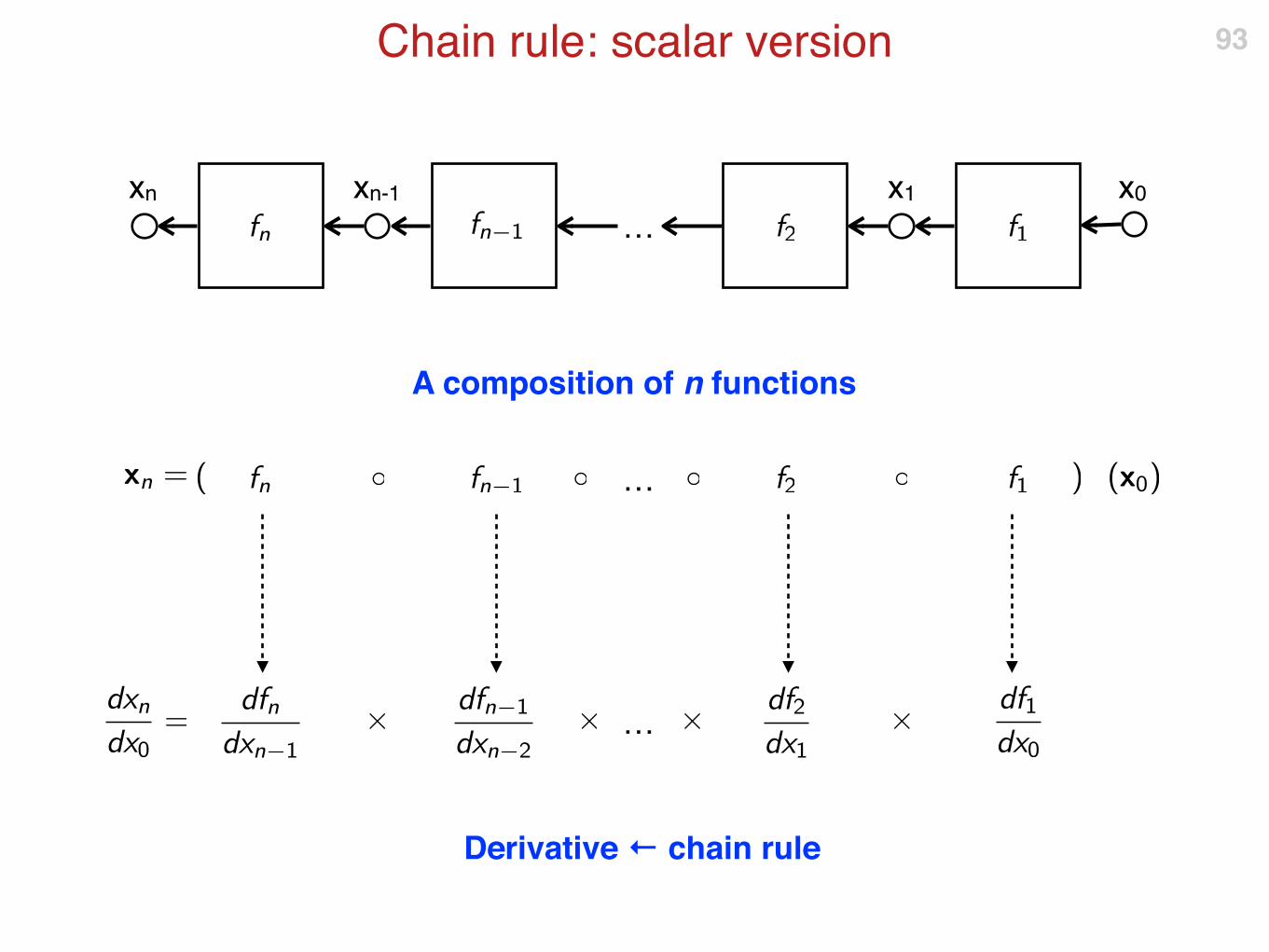
Chain rule: scalar version 93

xn x1

…

x0xn-1

…

…

A composition of n functions

Derivative ← chain rule

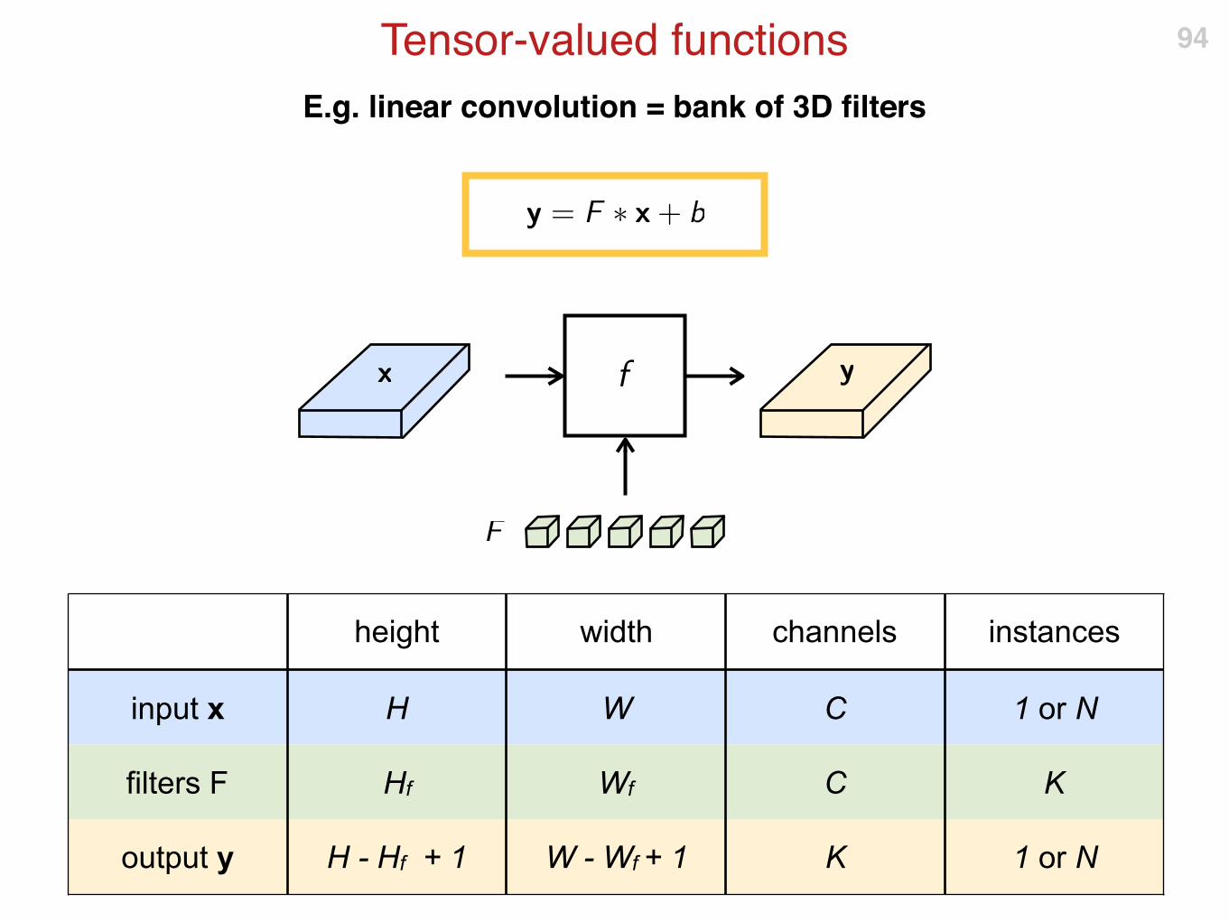
E.g. linear convolution = bank of 3D filters

Tensor-valued functions 94

height width channels instances

input x H W C 1 or N

filters F Hf Wf C K

output y H - Hf + 1 W - Wf + 1 K 1 or N

Vector representation 95

3D tensors

vectors

vec

Derivative of tensor-valued functions 96

Derivative (Jacobian): every output element w.r.t. every input element!

The vec operator allows us to use a familiar matrix notation for the derivatives

Using vec() and matrix notation

Chain rule: tensor version 97

xn x1

…

x0xn-1

…

…

The (unbearable) size of tensor derivatives 98

32 ⨉ 32 ⨉ 512

32 ⨉ 32 ⨉ 512

275 B elements

1 TB of memoryrequired !!

The size of these Jacobian matrices is huge. Example:

Unless the output is a scalar 99

Now the Jacobian has the same size as x. Example:

1 ⨉ 1 ⨉ 1

32 ⨉ 32 ⨉ 512

Just 2MB of memory

524K elements

Scalar

This is always the case if the last layer is the loss function

Assumed xn is a scalar (e.g. loss)

Backpropagation 100

xn x1

…

x0xn-1

…

…

uber matricesdo not explicitly compute

small explicitly compute

compute this first !

Assumed xn is a scalar (e.g. loss)

Backpropagation 101

xn x1

…

x0xn-1

…

…

uber matricesdo not explicitly compute

small explicitly compute

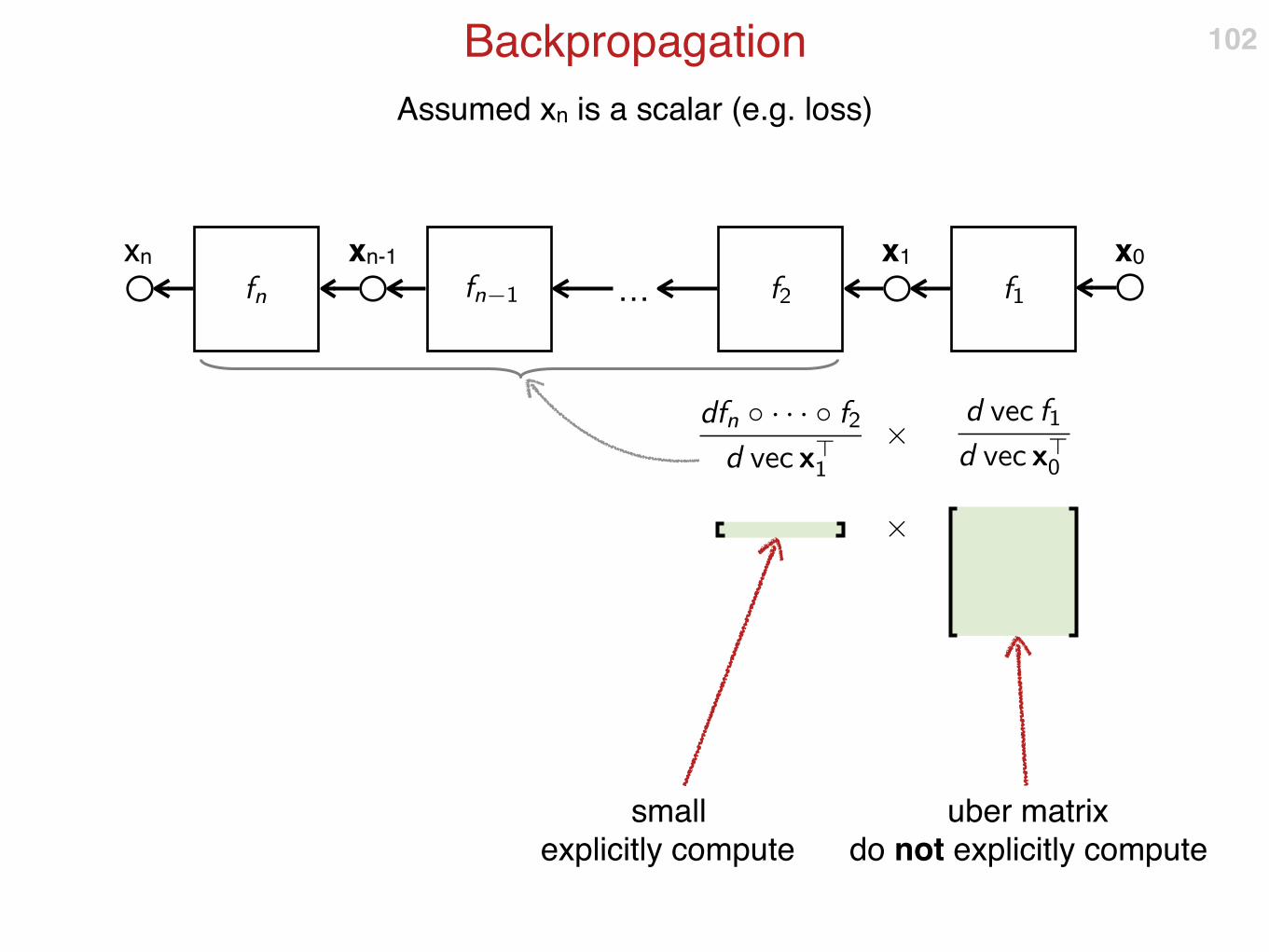
Assumed xn is a scalar (e.g. loss)

Backpropagation 102

xn x1

…

x0xn-1

uber matrixdo not explicitly compute

small explicitly compute

Assumed xn is a scalar (e.g. loss)

Backpropagation 103

xn x1

…

x0xn-1

small explicitly compute

The “BP-transpose” function

Projected function derivative 104

z y x

function projected

onto p projected function

derivative

An “equivalent circuit” is obtained by introducing a transposed function fT

BP induces a “transposed” network

Backpropagation network 105

xn x1

…

x0xn-1

dxn dx1

…dx0dxn-1

whereNote: the BP network is linearin dx1, …, dxn-1,dxn. Why?

BP induces a “transposed” network

Backpropagation network 106

xnx1

…x0 xn-1

dxndx1

…dx0 dxn-1

forward

backward

Interpretation of vector-matrix product in BP

Projected function derivative 107

z y x

function projected

onto p

projected function

derivative

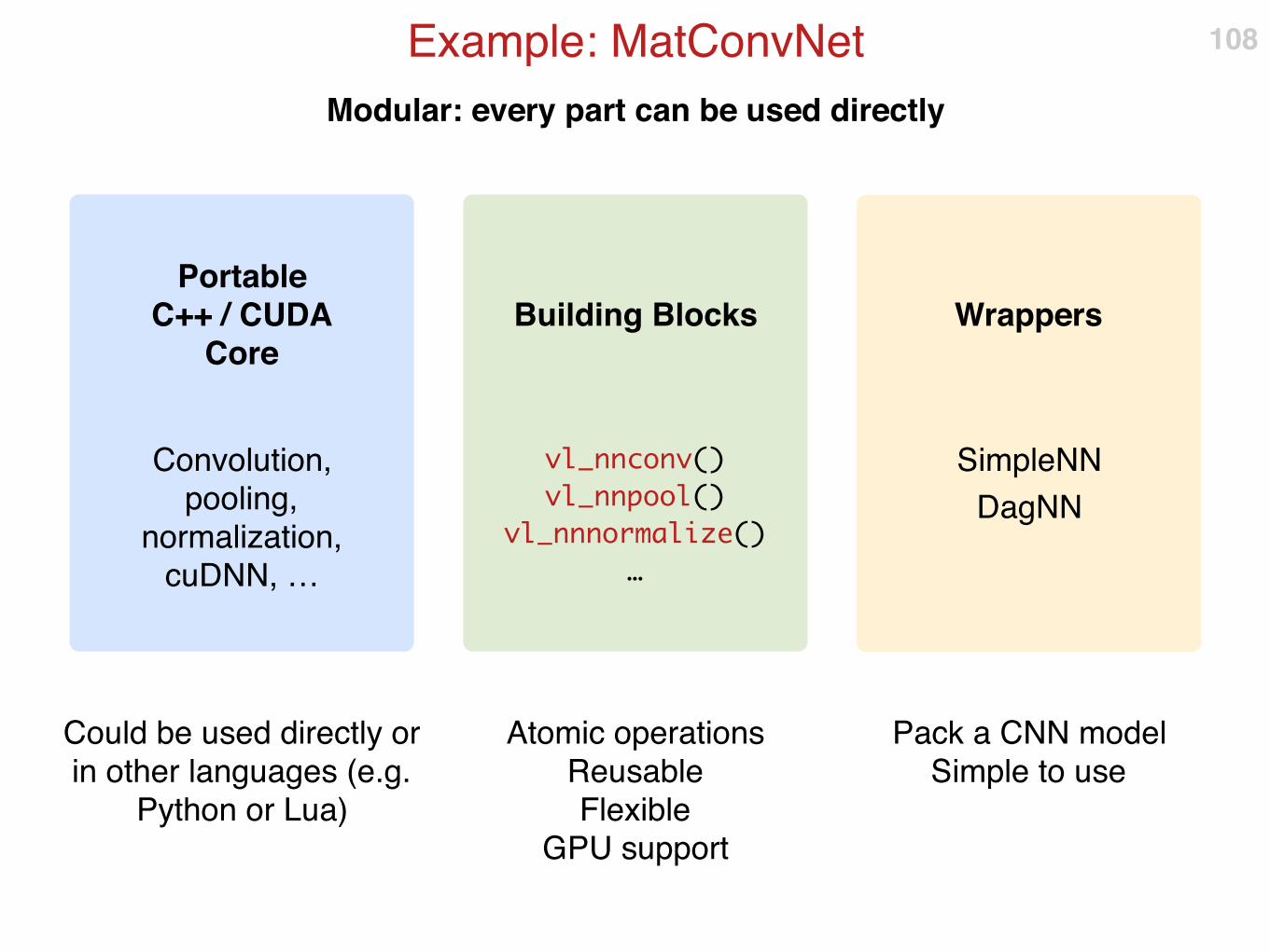
Modular: every part can be used directly

Example: MatConvNet 108

Portable C++ / CUDA

Core

Convolution, pooling,

normalization, cuDNN, …

Could be used directly or in other languages (e.g.

Python or Lua)

Wrappers

SimpleNN

DagNN

Pack a CNN model Simple to use

Building Blocks

vl_nnconv()

vl_nnpool()

vl_nnnormalize()

…

Atomic operationsReusable Flexible

GPU support

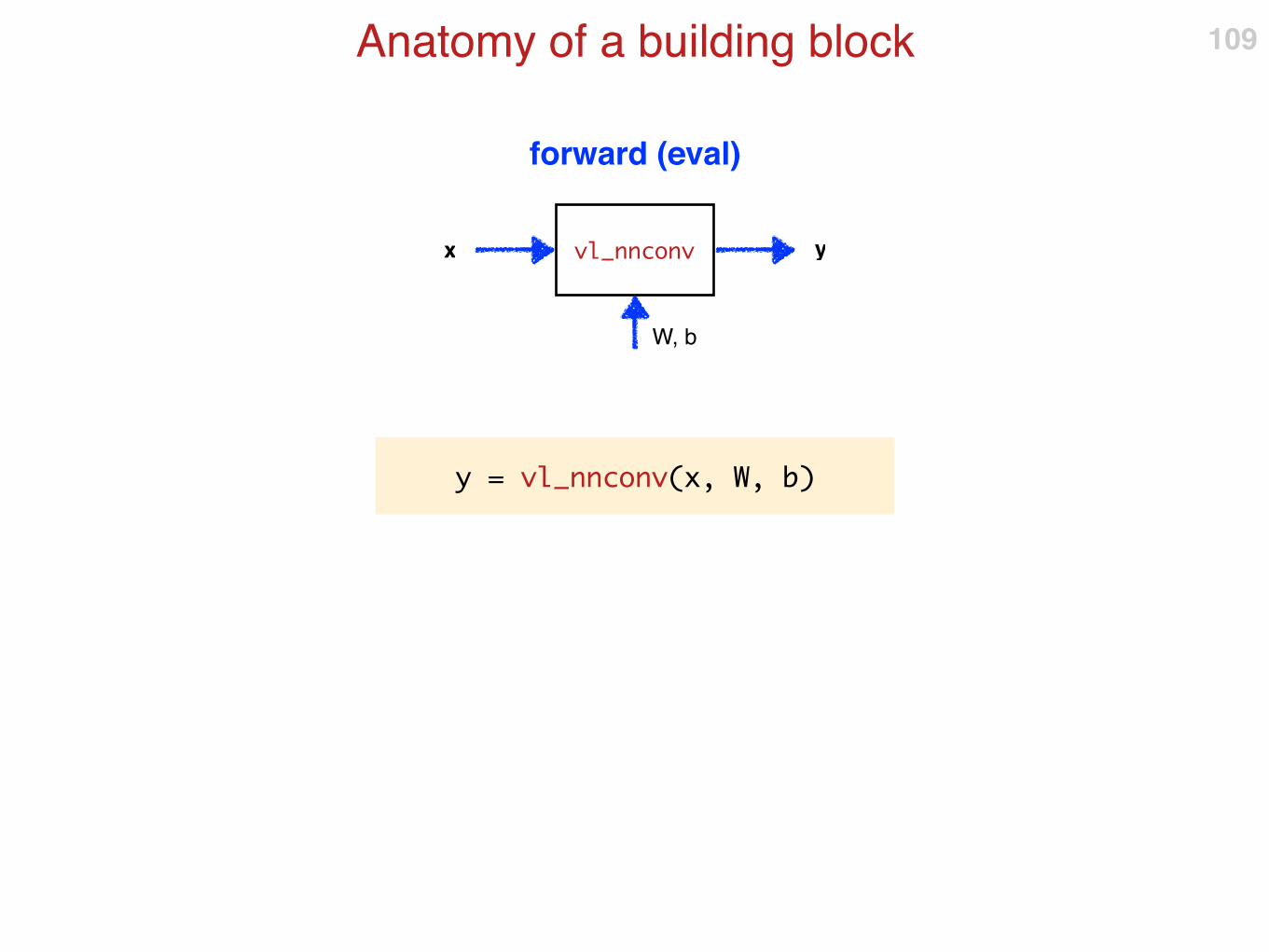
Anatomy of a building block 109

vl_nnconv

W, b

x y

y = vl_nnconv(x, W, b)

forward (eval)

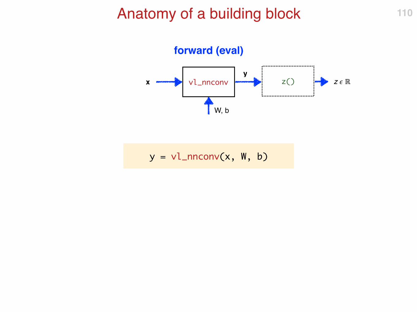
Anatomy of a building block 110

vl_nnconv

W, b

xy

z() z � ℝ

forward (eval)

y = vl_nnconv(x, W, b)

Anatomy of a building block 111

vl_nnconv

W, b

xy

y = vl_nnconv(x, W, b)

z() z � ℝ

vl_nnconv z()

dz

dydz

dx

dz

dW

dz

db

dzdx = vl_nnconv(x, W, b, dzdy)

backward (backprop)

forward (eval)

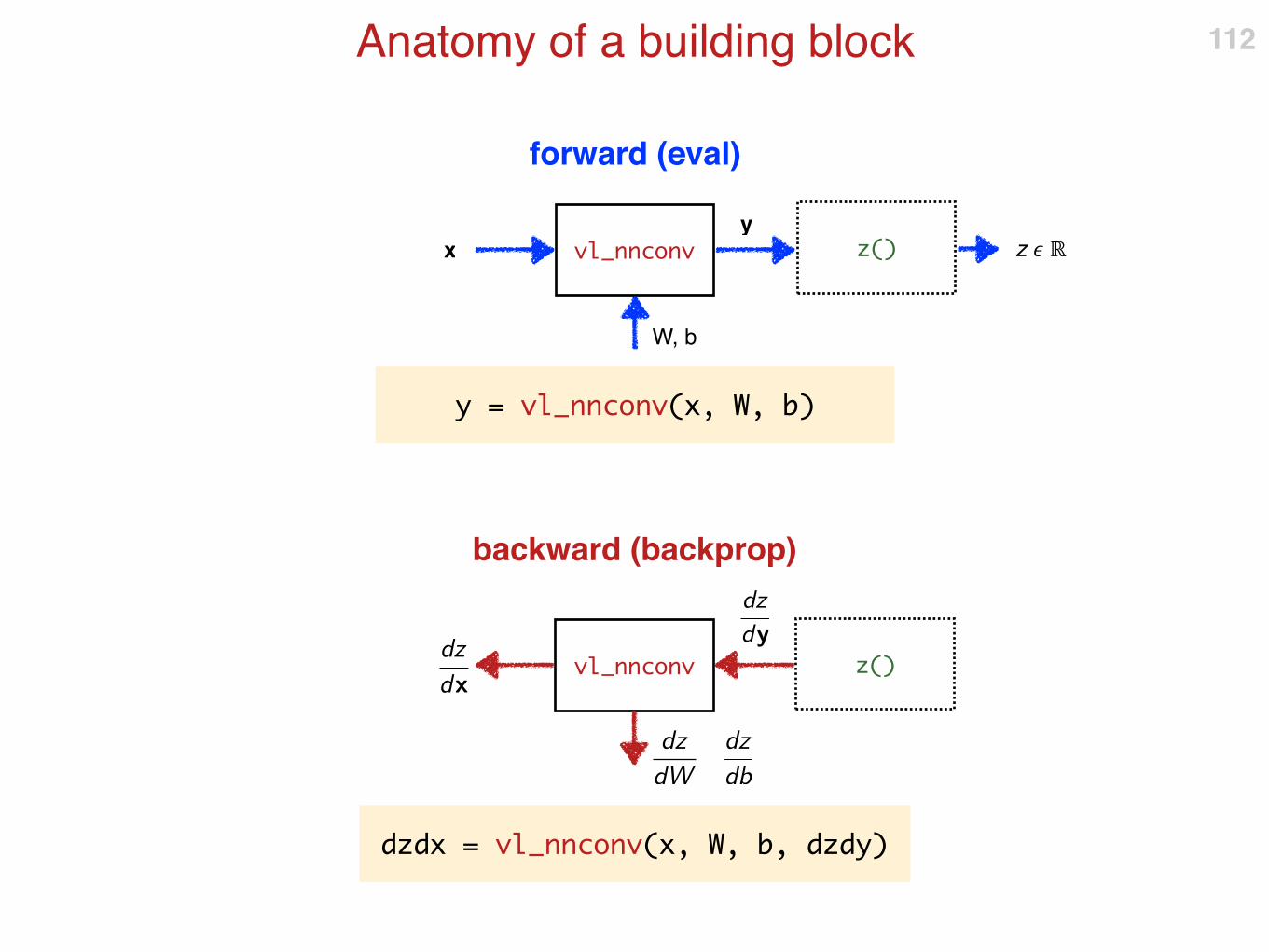
Anatomy of a building block 112

vl_nnconv

W, b

xy

y = vl_nnconv(x, W, b)

z() z � ℝ

vl_nnconv z()

dz

dydz

dx

dz

dW

dz

db

dzdx = vl_nnconv(x, W, b, dzdy)

backward (backprop)

forward (eval)

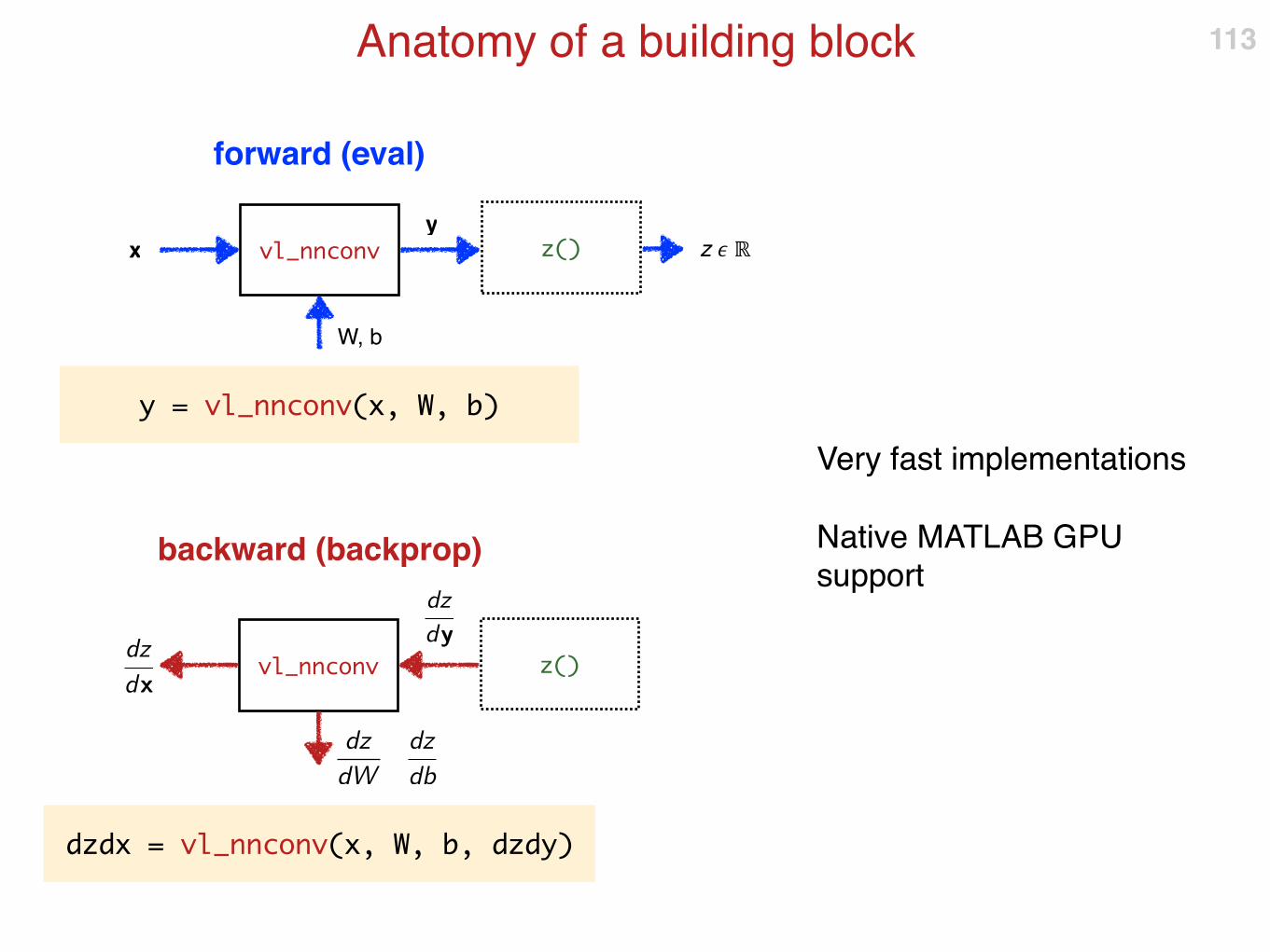
Anatomy of a building block

Very fast implementations

Native MATLAB GPU support

113

vl_nnconv

W, b

xy

y = vl_nnconv(x, W, b)

z() z � ℝ

vl_nnconv z()

dz

dydz

dx

dz

dW

dz

db

dzdx = vl_nnconv(x, W, b, dzdy)

backward (backprop)

forward (eval)

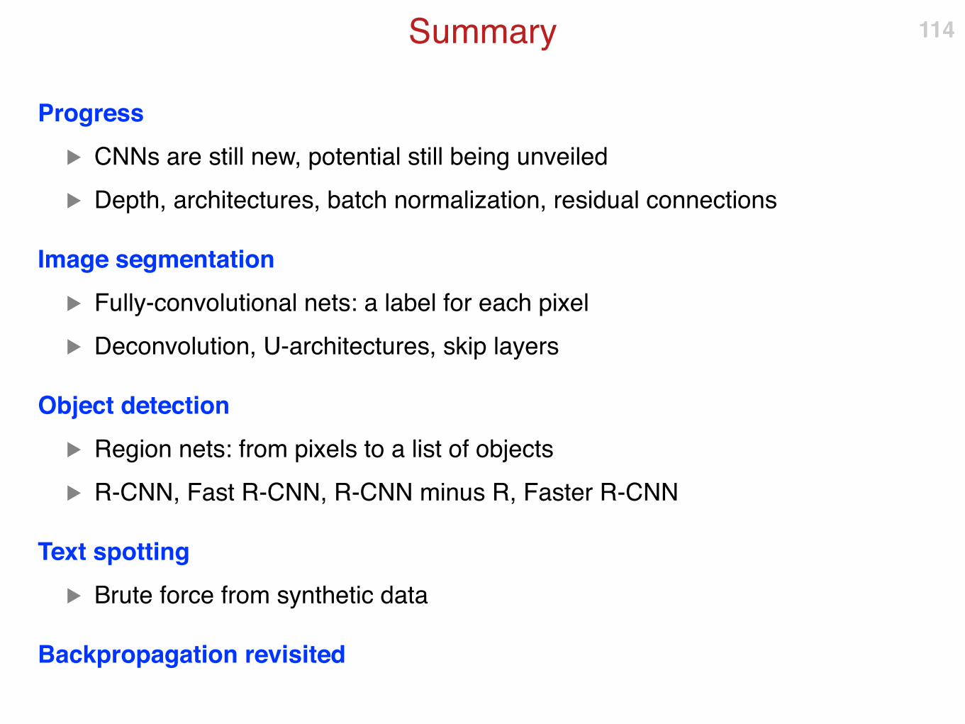
Summary

Progress

▶ CNNs are still new, potential still being unveiled

▶ Depth, architectures, batch normalization, residual connections

Image segmentation

▶ Fully-convolutional nets: a label for each pixel

▶ Deconvolution, U-architectures, skip layers

Object detection

▶ Region nets: from pixels to a list of objects

▶ R-CNN, Fast R-CNN, R-CNN minus R, Faster R-CNN

Text spotting

▶ Brute force from synthetic data

Backpropagation revisited

114